fys-geo 4500 filefys-geo 4500
TRANSCRIPT

FYS-GEO 4500 Galen Gisler, Physics of Geological Processes, University of Oslo Autumn 2011
FYS-GEO 4500
Lecture Notes #7Finite Volume Methods for Nonlinear Systems
Wednesday, 26 October 2011

FYS-GEO 4500 Galen Gisler, Physics of Geological Processes, University of Oslo Autumn 2011
2
Where we are todaydate Topic Chapter in
LeVeque123456
78
91011
12
1.Sep 2011 introduction to conservation laws, Clawpack 1 & 2
15.Sep 2011 the Riemann problem, characteristics 3 & 5
22.Sep 2011 finite volume methods for linear systems, high resolution 4 & 6
29.Sep 2011 boundary conditions, accuracy, variable coeff. 7,8, part 9
6.Oct 2011 nonlinear conservation laws, finite volume methods 11 & 12
13.Oct 2011 nonlinear equations & systems 13 & 14
20.Oct 2011 no lecture
27.Oct 2011 finite volume methods for nonlinear systems 15,16,17
3.Nov 2011 multidimensional systems and source terms, etc. 18, 19, 20, 21
10.Nov 2011 no lecture
17.Nov 2011 waves in elastic media 22
24.Nov 2011 unfinished business: capacity functions, source terms, project plansunfinished business: capacity functions, source terms, project plans
1.Dec 2011 student presentations
8.Dec 2011 no lecture
15.Dec 2011 FINAL REPORTS DUE
Wednesday, 26 October 2011

FYS-GEO 4500 Galen Gisler, Physics of Geological Processes, University of Oslo Autumn 2011
Other topics in Gas Dynamics
Wednesday, 26 October 2011

FYS-GEO 4500 Galen Gisler, Physics of Geological Processes, University of Oslo Autumn 2011
De Laval Nozzle
Invented by the Swedish engineer Gustaf de Laval in 1897.
This nozzle is the basis of how jet engines and rocket engines work.
The converging-diverging profile, with a sufficient difference in pressure between the reservoir and the exhaust, results in a smooth transition from subsonic to supersonic flow.
4
Wednesday, 26 October 2011

FYS-GEO 4500 Galen Gisler, Physics of Geological Processes, University of Oslo Autumn 2011
How does a deLaval nozzle work?
v2
2+ γ
γ −1⎛⎝⎜
⎞⎠⎟pρ= constant along a streamline,
Bernoulli’s equation says that, for steady flow of a gas (ignoring gravity),
Suppose we have a reservoir at high pressure connected via a pipe to a medium at much lower pressure.
Then there is a maximum velocity at steady flow given by:
vmax = c02
γ 0 −1
where c0 and γ0 refer to the thermodynamic conditions in the reservoir (where v=0), and this maximum value is obtained when the gas flows out into a vacuum (p=0).
= v2
2+ cs
2
γ −1 for an ideal gas.
5
Wednesday, 26 October 2011

FYS-GEO 4500 Galen Gisler, Physics of Geological Processes, University of Oslo Autumn 2011
How does a deLaval nozzle work?
Using where c is the local sound speed throughout the system, we get
Euler’s equation gives us the relation between v and ρ along a streamline:
vdv = dpρ.
dp = c2ρ,
d ρv( )dv
= ρ 1− v2
c2⎛⎝⎜
⎞⎠⎟,
indicating that the maximum possible mass flux ρv obtains when v is equal to the local sound speed. By continuity, the flux is constant throughout the pipe, including the narrowest point.
For the ideal gas, the flux is
ρv = pp0
⎛⎝⎜
⎞⎠⎟
1/γ2γγ −1
p0ρ0 1−pp0
⎛⎝⎜
⎞⎠⎟
γ −1( )/γ⎡
⎣⎢⎢
⎤
⎦⎥⎥
6
Wednesday, 26 October 2011

FYS-GEO 4500 Galen Gisler, Physics of Geological Processes, University of Oslo Autumn 2011
Velocity increases throughout the nozzle
The maximum discharge rate is reached, if ever, at the narrowest point of a nozzle.
If the pressure at this point is less than 0.53 p0 (in air) or less than 0.6 p0 (in a nearly isothermal gas), the flow speed equals the sound speed at that point. The nozzle throat is the transition from subsonic to supersonic flow.
The velocity continues to increase through the diverging part of the nozzle, by continuity:
ρv = pp0
⎛⎝⎜
⎞⎠⎟
1/γ2γγ −1
p0ρ0 1−pp0
⎛⎝⎜
⎞⎠⎟
γ −1( )/γ⎡
⎣⎢⎢
⎤
⎦⎥⎥,
0
0.175
0.350
0.525
0.700
0 0.25 0.50 0.75 1.00
γ = 1.4
γ = 1.01
p / p0
ρvρ0c0
7
d ρv( )dv
= ρ 1− v2
c2⎛⎝⎜
⎞⎠⎟,
Wednesday, 26 October 2011

FYS-GEO 4500 Galen Gisler, Physics of Geological Processes, University of Oslo Autumn 2011
De Laval Nozzle
Invented by the Swedish engineer Gustaf de Laval in 1897.
This nozzle is the basis of how jet engines and rocket engines work.
The converging-diverging profile, with a sufficient difference in pressure between the reservoir and the exhaust, results in a smooth transition from subsonic to supersonic flow.
8
d ρv( )dv
= ρ 1− v2
c2⎛⎝⎜
⎞⎠⎟,
Wednesday, 26 October 2011

Simulation of an erupting column using the Sage
multi-material code 600 m ice
3.2 km basalt
Magma column, 98% basalt, 2% water (by mass)1500 K, 1 kbar
Wednesday, 26 October 2011

Simulation of an erupting column using the Sage
multi-material code 600 m ice
3.2 km basalt
Magma column, 98% basalt, 2% water (by mass)1500 K, 1 kbar
Wednesday, 26 October 2011

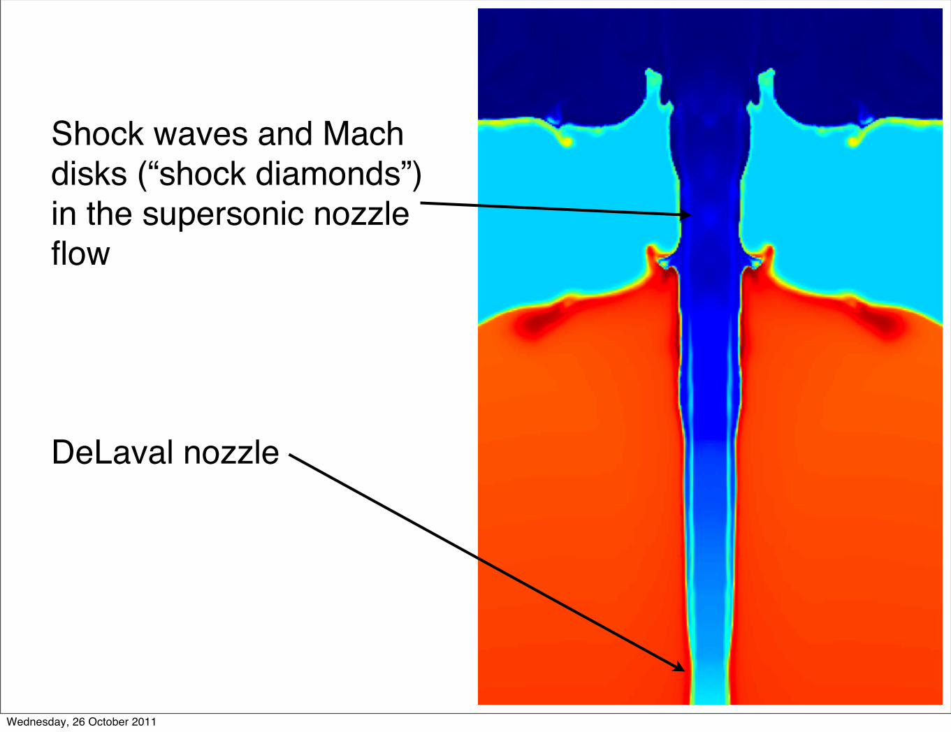
Shock waves and Mach disks (“shock diamonds”) in the supersonic nozzle flow
DeLaval nozzle
Wednesday, 26 October 2011

Shock waves and Mach disks (“shock diamonds”) in the supersonic nozzle flow
DeLaval nozzle
Wednesday, 26 October 2011
Shock waves and Mach disks (“shock diamonds”) in the supersonic nozzle flow
DeLaval nozzle
Wednesday, 26 October 2011

FYS-GEO 4500 Galen Gisler, Physics of Geological Processes, University of Oslo Autumn 2011
Multifluid problems and other equations of state: How to do in Clawpack?
The easiest multi-fluid case is when you have two ideal gases with different values of γ. Then you set up the Riemann problem at the interface between the two fluids with right and left values for γ. Things get complicated when mixing occurs.
Other analytical or tabular equations of state can also be incorporated into a finite volume conservative scheme. Sage, for example, uses the Sesame library of tabular equations of state for lots of materials. The Sesame library, developed at Los Alamos National Laboratory, contains mostly industrial materials, with a few materials of geological interest.
Leveque gives lots of references to papers in which Riemann solvers are developed for other equations of state in his section 14.15. Some of these will be worth looking into for geological applications.
11
Wednesday, 26 October 2011

FYS-GEO 4500 Galen Gisler, Physics of Geological Processes, University of Oslo Autumn 2011
The Mie-Grüneisen-Lemons Multiphase EOS
This is an equation of state proposed by Don Lemons based on Mie-Grüneisen theory for substances that undergo relatively simple phase transitions from solid to liquid to gas.
In common with the van der Waals EOS (see Leveque, ch 14.15 and 16.3.2), this EOS results in loss of hyperbolicity unless Maxwell constructions are used.
This EOS has substance-specific constants
p = ΓcvρT + 3Bn − m( )
ρρ0
⎛⎝⎜
⎞⎠⎟
n+33− ρ
ρ0
⎛⎝⎜
⎞⎠⎟
m+33
⎡
⎣
⎢⎢⎢
⎤
⎦
⎥⎥⎥
e = cvT + 9Bρ0 n − m( )
1n
ρρ0
⎛⎝⎜
⎞⎠⎟
n3− 1m
ρρ0
⎛⎝⎜
⎞⎠⎟
m3− 1n+ 1m
⎡
⎣
⎢⎢⎢
⎤
⎦
⎥⎥⎥
n,m,ρ0 ,B,Γ
12
Wednesday, 26 October 2011

FYS-GEO 4500 Galen Gisler, Physics of Geological Processes, University of Oslo Autumn 2011
Dusty Gases, Anyone?
Marica Pelanti, a student of Randy Leveque, developed a code based on Clawpack for volcanic jets using a dusty gas model.
See*: Pelanti & Leveque, "High-Resolution Finite Volume Methods for Dusty Gas Jets and Plumes", SIAM J. Sci. Comput. 28 (2006) 1335-1360.
Their model was multifluid: Euler equations for the gas, and a pressure-less fluid for the dust, coupled together by drag and heat transfer.
Or… we could try a single-fluid dusty gas equation of state.
* http://www-roc.inria.fr/bang/Pelanti/
13
Wednesday, 26 October 2011

FYS-GEO 4500 Galen Gisler, Physics of Geological Processes, University of Oslo Autumn 2011
What happens when we add dust to gas?
The speed of acoustic waves in a general medium is,
which for an ideal gas is
Assuming the dust remains coupled to the gas (via Stokes drag), for a little loading the density increases without the pressure changing much.
Thus the speed of sound decreases. In fact, it does so dramatically.
cs =∂p∂ρ
⎛⎝⎜
⎞⎠⎟isentropic
cs =γ pρ
14
Wednesday, 26 October 2011

FYS-GEO 4500 Galen Gisler, Physics of Geological Processes, University of Oslo Autumn 2011
An equation of state for a dusty gas*
One version of a dusty-gas equation of state is:
where K is the mass concentration and Z is the volume fraction of solid particles.
These are related through where is the particle solid density.
The speed of sound is then
where the ratio of specific heats for the mixture is
The specific heat of the dust particles is Csp and Cv is the specific heat at constant volume of the gas.
p = (1− K )(1− Z )
ρRT ,
cds =Γp
ρ(1− Z )
Γ =γCv (1− K )+CspKCv (1− K )+CspK
.
K = Zρs
ρ,
*from Vishwakarma, Nath, & Singh (2008), Physica Scripta 78 035402.http://stacks.iop.org/PhysScr/78/035402
ρs
15
Wednesday, 26 October 2011

FYS-GEO 4500 Galen Gisler, Physics of Geological Processes, University of Oslo Autumn 2011
Density increases more rapidly than pressure as the dust content increases
ρ
Z (volume fraction of dust)
pressure right scaledensity left scale
p
2.0
10.0
1.0
3.0
4.0
5.0
6.0
7.0
(g/cc)
0.00
0.01
0.10
1.00
1E-06 1E-05 1E-04 1E-03 1E-02 1E-01 1E+001E+00
(bar)
Assumptions: spherical dust particles
150 µ radius, 2.5 g/cc density, specific heat 0.92 J/g Kair at density 1.204e-3 g/cc, temperature 293 K
16
Wednesday, 26 October 2011

FYS-GEO 4500 Galen Gisler, Physics of Geological Processes, University of Oslo Autumn 2011
Adding 0.1% dust (by volume) to air cuts the speed of sound in half, and the mixture approaches isothermal
0.6
0.8
1.0
1.2
1.4
1E-06 1E-05 1E-04 1E-03 1E-02 1E-01 1E+001E+00
0
100
200
300
400
1E-06 1E-05 1E-04 1E-03 1E-02 1E-01 1E+001E+00
speed of sound in the
dusty gas (m/s)
ratio of specific heats of the mixture
Γ
volume fraction occupied by dust particles
Assumptions: spherical dust particles
150 µ in radius, 2.5 g/cc density, specific heat 0.92 J/g Kair at density 1.204e-3 g/cc, temperature 293 K
17
Wednesday, 26 October 2011

FYS-GEO 4500 Galen Gisler, Physics of Geological Processes, University of Oslo Autumn 2011
Shocks can be stronger in dusty gases
The maximum ratio of upstream to downstream densities across a shock is (see Landau & Lifshitz, Fluid Dynamics)
For a diatomic gas (like air),
For a dusty gas, can be arbitrarily large. At
ρuρd
= γ +1γ −1
.
γ = 1.4, so ρuρd
= 6.
γ ⇒1, so ρuρd
γ = 1.01, ρuρd
= 201.
18
Wednesday, 26 October 2011
FYS-GEO 4500 Galen Gisler, Physics of Geological Processes, University of Oslo Autumn 2011
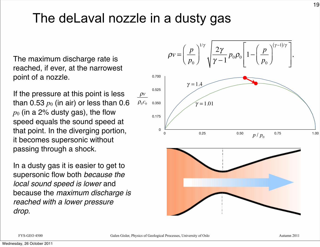
The deLaval nozzle in a dusty gas
The maximum discharge rate is reached, if ever, at the narrowest point of a nozzle.
If the pressure at this point is less than 0.53 p0 (in air) or less than 0.6 p0 (in a 2% dusty gas), the flow speed equals the sound speed at that point. In the diverging portion, it becomes supersonic without passing through a shock.
In a dusty gas it is easier to get to supersonic flow both because the local sound speed is lower and because the maximum discharge is reached with a lower pressure drop.
ρv = pp0
⎛⎝⎜
⎞⎠⎟
1/γ2γγ −1
p0ρ0 1−pp0
⎛⎝⎜
⎞⎠⎟
γ −1( )/γ⎡
⎣⎢⎢
⎤
⎦⎥⎥,
0
0.175
0.350
0.525
0.700
0 0.25 0.50 0.75 1.00
γ = 1.4
γ = 1.01
p / p0
ρvρ0c0
19
Wednesday, 26 October 2011

FYS-GEO 4500 Galen Gisler, Physics of Geological Processes, University of Oslo Autumn 2011
Vents, kimberlite pipes, volcanos, and geysers may be natural deLaval nozzles for a dusty gas
1 cm
Hydro
the
rmal altera
tion
an
d f
ractu
rin
g
Bo
reh
ole
Sedimentpipes
Slumping
Zeolite
Vent sandstone(Facies unit I)
Sediment breccia(Facies unit III)
Zeolite-cementedsandstone (Faciesunit II)
100 m
100 m
200 m
300 m
0 m
Facies unit II
Erosion profile
20
Wednesday, 26 October 2011

FYS-GEO 4500 Galen Gisler, Physics of Geological Processes, University of Oslo Autumn 2011
Finite Volume Methods for Nonlinear Systems
(Chapter 15 in Leveque)
Wednesday, 26 October 2011

FYS-GEO 4500 Galen Gisler, Physics of Geological Processes, University of Oslo Autumn 2011
Once again, we extend from what we’ve learned for linear systems of equations
We intend to solve the nonlinear conservation law
using a method that is in conservative form:
and yielding a weak solution to this conservation law. To get the correct weak solution we must use an appropriate entropy condition.
qt + f (q)x = 0
Qin+1 =Qi
n − ΔtΔx
Fi+1/2n − Fi−1/2
n( )
22
Wednesday, 26 October 2011

FYS-GEO 4500 Galen Gisler, Physics of Geological Processes, University of Oslo Autumn 2011
Recall Godunov’s method:
Given a set of cell quantities at time n:
1. Solve the Riemann problem at to obtain
2. Define the flux:
3. Apply the flux differencing formula:
This will work for any general system of conservation laws. Only the formulation of the Riemann problem itself changes with the system.
Fi−1/2n = f Qi−1/2
↓( )
Qin
Qi−1/2↓ = q↓(Qi−1
n ,Qin )xi−1/2
Qin+1 =Qi
n − ΔtΔx
Fi+1/2n − Fi−1/2
n( )
23
Wednesday, 26 October 2011

FYS-GEO 4500 Galen Gisler, Physics of Geological Processes, University of Oslo Autumn 2011
In terms of the REA scheme we have discussed
1. Reconstruct a piece-wise linear function from the cell averages.
with the property that TV(q) ≤ TV(Q)
2. Evolve the hyperbolic equation (approximately) with this function to obtain a later-time function, by solving Riemann problems at the interfaces.
3. Average this function over each grid cell to obtain new cell averages.
qn (x,tn+1)
The reconstruction step depends on the slope limiter that is chosen, and should be subject to TVD constraints. The other two steps do not affect TVD.
qn (x,tn ) =Qin +σ i
n (x − xi ) for x in cell i
Qi
n+1 = 1Δx
qn (x,tn+1)xi−1/2
xi+1/2∫ dx
evolve
reconstruct
average
24
Wednesday, 26 October 2011
FYS-GEO 4500 Galen Gisler, Physics of Geological Processes, University of Oslo Autumn 2011
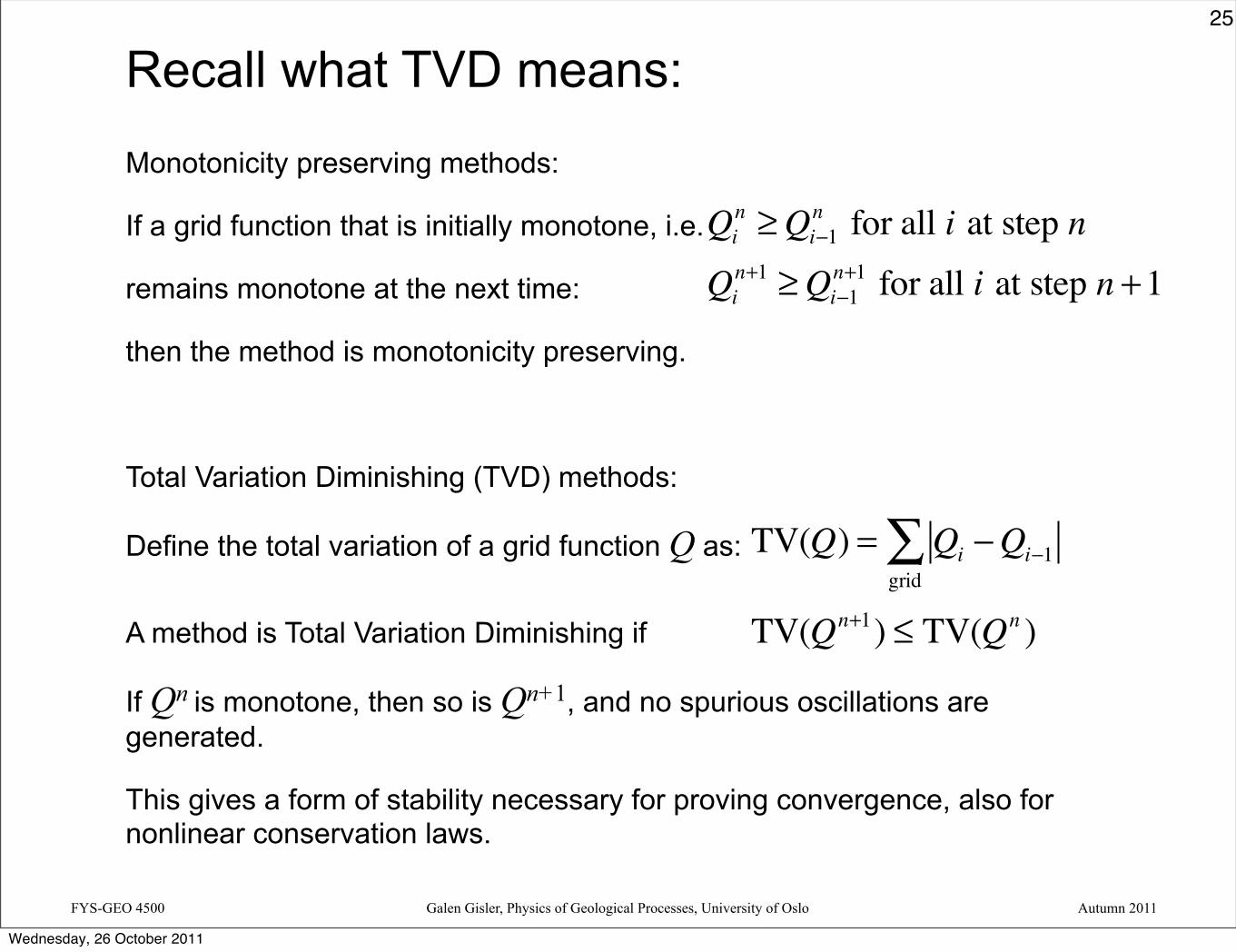
Recall what TVD means:
Monotonicity preserving methods:
If a grid function that is initially monotone, i.e.
remains monotone at the next time:
then the method is monotonicity preserving.
Total Variation Diminishing (TVD) methods:
Define the total variation of a grid function Q as:
A method is Total Variation Diminishing if
If Qn is monotone, then so is Qn+1, and no spurious oscillations are generated.
This gives a form of stability necessary for proving convergence, also for nonlinear conservation laws.
TV(Q) = Qi −Qi−1grid∑
TV(Qn+1) ≤ TV(Qn )
Qin ≥Qi−1
n for all i at step nQi
n+1 ≥Qi−1n+1 for all i at step n +1
25
Wednesday, 26 October 2011

FYS-GEO 4500 Galen Gisler, Physics of Geological Processes, University of Oslo Autumn 2011
For advection, the REA algorithm gives us:We update the advection equation by
where the slope is given by
where is the flux limiter function.
Choices for the flux limiter are:
Qin+1 =Qi
n − uΔtΔx
Qin −Qi−1
n( )− 12uΔtΔx
Δx − uΔt( ) σ in −σ i−1
n( )
σ in = Qi+1
n −Qin
Δx⎛⎝⎜
⎞⎠⎟φin
φ
φ(θ) = 0φ(θ) = 1φ(θ) = θ
φ(θ) = 12(1+θ)
φ(θ) = minmod(1,θ)φ(θ) = max(0,min(1,2θ),min(2,θ))φ(θ) = max(0,min((1+θ) / 2,2,2θ))
φ(θ) = (θ + θ )(1+ θ )
upwind:
Lax-Wendroff:
Beam-Warming:
Fromm:
minmod:
superbee:
MC:
van Leer:
θin = Qi
n −Qi−1n
Qi+1n −Qi
n
26
Wednesday, 26 October 2011

FYS-GEO 4500 Galen Gisler, Physics of Geological Processes, University of Oslo Autumn 2011
Slope limiters and flux limiters
The slope limiter formula for advection is:
The flux limiter formulation for advection is:
with the flux:
Qin+1 =Qi
n − uΔtΔx
Qin −Qi−1
n( )− 12uΔtΔx
Δx − uΔt( ) σ in −σ i−1
n( )
Qin+1 =Qi
n − ΔtΔx
Fi+1/2n − Fi−1/2
n( )
Fi−1/2n = uQi−1
n + 12u(Δx − uΔt)σ i−1
n
27
Wednesday, 26 October 2011

FYS-GEO 4500 Galen Gisler, Physics of Geological Processes, University of Oslo Autumn 2011
Wave limiters:
Let:
Upwind formula:
Lax-Wendroff formula:
High-resolution method:
where
xi−1/2
Qin
Wi−1/2Qi−1
n
Wi−1/2 =Qin −Qi−1
n
Qi
n+1 =Qin − uΔt
ΔxWi−1/2
Qi
n+1 =Qin − uΔt
ΔxWi−1/2 −
ΔtΔx
Fi+1/2 − Fi−1/2( )
Fi−1/2 =
121− uΔt
Δx⎛⎝⎜
⎞⎠⎟uWi−1/2
Fi−1/2 =
121− u Δt
Δx⎛⎝⎜
⎞⎠⎟uW i−1/2 ,
W i−1/2 = φi−1/2Wi−1/2 .
28
Wednesday, 26 October 2011

FYS-GEO 4500 Galen Gisler, Physics of Geological Processes, University of Oslo Autumn 2011
Extension to linear systems
Approach 1:
Diagonalise the system to
Apply the scalar algorithm to each component separately.
Approach 2:
Solve the linear Riemann problem to decompose into a number of waves.
Apply a wave limiter to each wave.
These approaches are equivalent.
But note that it is important to apply the limiters to the waves rather than to the original variables.
qt + Λqx = 0
Qin −Qi−1
n
xi−1/2 xi+1/2
Qin Qi+1
n
Wi−1/22
Wi−1/23
Wi+1/21
Qi−1n
Wi−1/21
29
Wednesday, 26 October 2011

FYS-GEO 4500 Galen Gisler, Physics of Geological Processes, University of Oslo Autumn 2011
Wave propagation methods
Solving the Riemann problem between cells i and i+1 gives the waves
and speeds . In the nonlinear case, an approximate solution is used.
These waves update the neighbouring cell averages via fluctuations, depending on sign of .
The waves also give the decomposition of the slopes
Apply the limiter to each wave to obtain
Use the limited waves in the second-order correction terms.
xi−1/2 xi+1/2
Qin Qi+1
n
Wi−1/22
Wi−1/23
Wi+1/21
Qi−1n
Wi−1/21
Qi −Qi−1 = Wi−1/2
p
p=1
m
∑ ,
si−1/2p
si−1/2p
Qi −Qi−1
Δx= 1ΔxWi−1/2
p
p=1
m
∑ ,
W i−1/2 = φi−1/2Wi−1/2 .
30
Wednesday, 26 October 2011

FYS-GEO 4500 Galen Gisler, Physics of Geological Processes, University of Oslo Autumn 2011
High-resolution wave-propagation scheme
The fluctuation notation is more useful in the nonlinear case:
where
represents the limited version of .
This is obtained by comparing with where
Fi−1/2n = 1
2si−1/2p 1− Δt
Δxsi−1/2p⎛
⎝⎜⎞⎠⎟W i−1/2
p
p=1
m
∑ Qi
n+1 =Qin − Δt
ΔxA−ΔQi+1/2 +A+ΔQi−1/2( )− Δt
ΔxFi+1/2 − Fi−1/2( )
W i−1/2p Wi−1/2
p
Wi−1/2p Wl−1/2
p
l =i −1 if si−1/2
p > 0i +1 if si−1/2
p < 0⎧⎨⎩⎪
31
Wednesday, 26 October 2011

FYS-GEO 4500 Galen Gisler, Physics of Geological Processes, University of Oslo Autumn 2011
Wave limiters for a system
is split into waves
We replace these waves with the limited versions
where , and .
Note that if then .
In the scalar case this reduces to
xi−1/2 xi+1/2
Qin Qi+1
n
Wi−1/22
Wi−1/23
Wi+1/21
Qi−1n
Wi−1/21
Qi −Qi−1 Wi−1/2p = α i−1/2
p ri−1/2p ,
Wi−1/2p = φ(θi−1/2
p )Wi−1/2p .
θi−1/2p = Wi−1/2
p ⋅Wl−1/2p
Wi−1/2p ⋅Wi−1/2p l =i −1 if si−1/2
p > 0i +1 if si−1/2
p < 0⎧⎨⎩⎪
ri−1/2p = rl−1/2
p θi−1/2p = α l−1/2
p
α i−1/2p
θi−1/2p = Wl−1/2
p
Wi−1/2p = Ql −Ql−1
Qi −Qi−1
32
Wednesday, 26 October 2011

FYS-GEO 4500 Galen Gisler, Physics of Geological Processes, University of Oslo Autumn 2011
The exact Riemann solver for the nonlinear problem is expensive, and requires an iterative solver…
Qin
xi−1/2
tn+1
Qi−1n
tn
ql
ql* qr
*
qr
u =ϕ l p( ) =ul +
2clγ −1
1− p / pl( )γ −12γ
⎡⎣⎢
⎤⎦⎥
if p ≤ pl
ul +2cl
2γ γ −1( )1− p / pl1+ β p / pl
⎡
⎣⎢⎢
⎤
⎦⎥⎥
if p ≥ pl
⎧
⎨
⎪⎪
⎩
⎪⎪
u =ϕr p( ) =ur −
2crγ −1
1− p / pr( )γ −12γ
⎡⎣⎢
⎤⎦⎥
if p ≤ pr
ur −2cr
2γ γ −1( )1− p / pr1+ β p / pr
⎡
⎣⎢⎢
⎤
⎦⎥⎥
if p ≥ pr
⎧
⎨
⎪⎪
⎩
⎪⎪
ϕ l pm( ) =ϕr pm( ) (p*,u*) ρl* = 1+ β p* / pl
p* / pl + β⎛⎝⎜
⎞⎠⎟ρl ; ρr
* = 1+ β p* / prp* / pr + β
⎛⎝⎜
⎞⎠⎟ρrSolving yields , then
In the rarefaction fan,
ρ ξ( ) = ρlγ
γ plu(ξ)− ξ( )2⎛
⎝⎜⎞⎠⎟
1/(γ −1)
p ξ( ) = plρl
γ
⎛⎝⎜
⎞⎠⎟ρ ξ( )γ
u ξ( ) = γ −1( )ul + 2 cl + ξ( )γ +1
.
33
Wednesday, 26 October 2011

FYS-GEO 4500 Galen Gisler, Physics of Geological Processes, University of Oslo Autumn 2011
Newton’s Method for finding a root of a functionNewton’s method aims at finding a root by extrapolating from the function’s slope at the point where each successive guess is taken. This is very robust, provided there are no intervening extrema.
Each successive guess is given by
where the slope k is chosen from
First guess
Second guess
Third guess
xn+1 = xn −f (xn )k
(a) k = ′f xn( )
(b) k =f xn( )− f xn−1( )
xn − xn−1
(c) k =f xn( )− f xm( )
xn − xm
tangent method
secant method; more convenient than the tangent method when the derivative is unavailable or difficult to compute.
regula falsi; m is the most recent guess in which the function has the opposite sign. This method always brackets the root and is therefore most robust, but generally a bit slower.
34
Wednesday, 26 October 2011
FYS-GEO 4500 Galen Gisler, Physics of Geological Processes, University of Oslo Autumn 2011
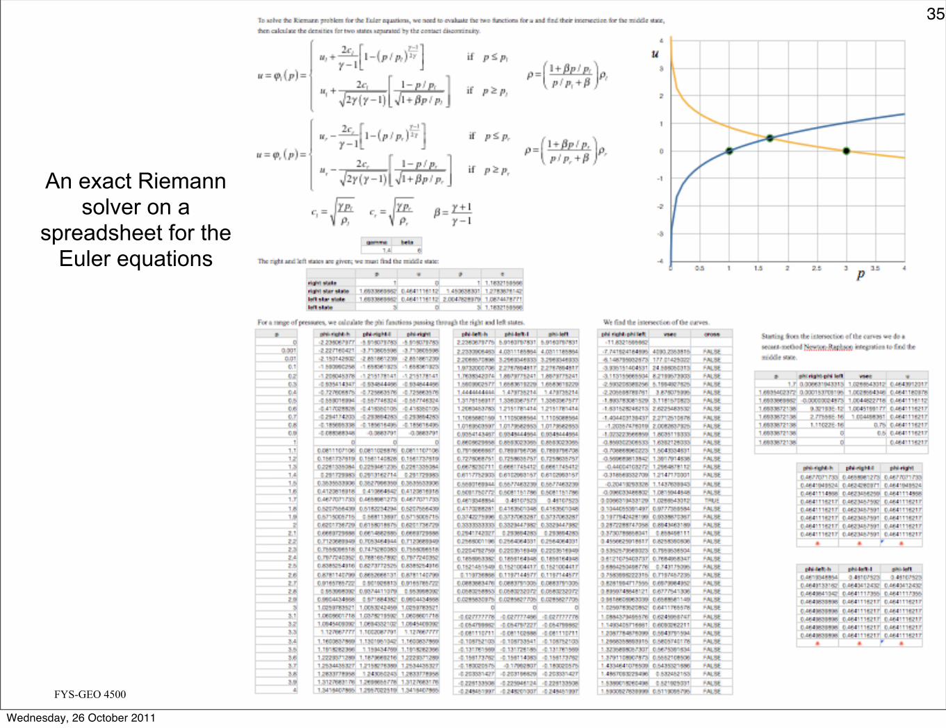
An exact Riemann solver on a
spreadsheet for the Euler equations
35
Wednesday, 26 October 2011

FYS-GEO 4500 Galen Gisler, Physics of Geological Processes, University of Oslo Autumn 2011
The exact Riemann solver for the nonlinear problem is expensive, and most of it is not necessary!
These are useful for exact solutions of certain problems.
But in simulations we only need the solution at the cell interface!
Qin
xi−1/2
tn+1
Qi−1n
tn
ql
ql* qr
*
qr
u =ϕ l p( ) =ul +
2clγ −1
1− p / pl( )γ −12γ
⎡⎣⎢
⎤⎦⎥
if p ≤ pl
ul +2cl
2γ γ −1( )1− p / pl1+ β p / pl
⎡
⎣⎢⎢
⎤
⎦⎥⎥
if p ≥ pl
⎧
⎨
⎪⎪
⎩
⎪⎪
u =ϕr p( ) =ur −
2crγ −1
1− p / pr( )γ −12γ
⎡⎣⎢
⎤⎦⎥
if p ≤ pr
ur −2cr
2γ γ −1( )1− p / pr1+ β p / pr
⎡
⎣⎢⎢
⎤
⎦⎥⎥
if p ≥ pr
⎧
⎨
⎪⎪
⎩
⎪⎪
ϕ l pm( ) =ϕr pm( ) (p*,u*) ρl* = 1+ β p* / pl
p* / pl + β⎛⎝⎜
⎞⎠⎟ρl ; ρr
* = 1+ β p* / prp* / pr + β
⎛⎝⎜
⎞⎠⎟ρrSolving yields , then
In the rarefaction fan,
ρ ξ( ) = ρlγ
γ plu(ξ)− ξ( )2⎛
⎝⎜⎞⎠⎟
1/(γ −1)
p ξ( ) = plρl
γ
⎛⎝⎜
⎞⎠⎟ρ ξ( )γ
u ξ( ) = γ −1( )ul + 2 cl + ξ( )γ +1
.
36
Wednesday, 26 October 2011
FYS-GEO 4500 Galen Gisler, Physics of Geological Processes, University of Oslo Autumn 2011
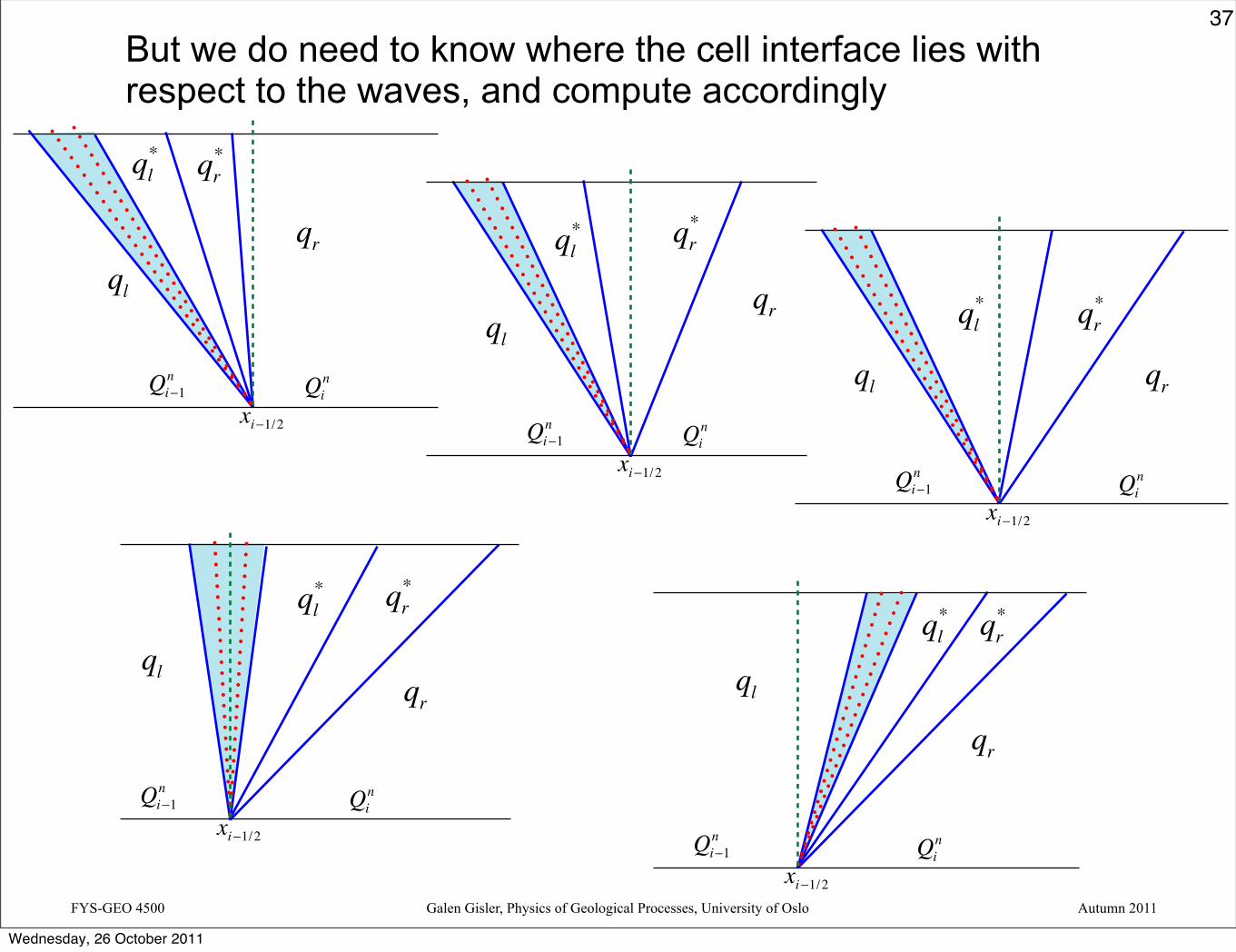
But we do need to know where the cell interface lies with respect to the waves, and compute accordingly
Qin
xi−1/2Qi−1
n
ql
ql* qr
*
qr
Qin
xi−1/2Qi−1
n
ql
ql* qr
*
qrQi
n
xi−1/2Qi−1
n
ql
ql* qr
*
qr
Qin
xi−1/2Qi−1
n
ql
ql* qr
*
qr
Qin
xi−1/2Qi−1
n
ql
ql* qr
*
qr
37
Wednesday, 26 October 2011

FYS-GEO 4500 Galen Gisler, Physics of Geological Processes, University of Oslo Autumn 2011
Wave interactions
Waves that interact with each other within a cell will not change the cell-interface values on the next time step provided the Courant number is less than 1.
Qin
xi−1/2Qi−1
n Qi+1n
xi+1/2
38
Wednesday, 26 October 2011

FYS-GEO 4500 Galen Gisler, Physics of Geological Processes, University of Oslo Autumn 2011
Riemann solvers in CLAWPACK
In CLAWPACK, the hyperbolic problem is specified by providing a Riemann solver with
Input: the value of q in each grid cell
Output: the solution to the Riemann problem at each cell interface:
The Waves for a system of m equations
The Speeds
The Fluctuations , for high-resolution corrections
Because the problem is solved entirely using Riemann solvers, you won’t see anything in the code that resembles the original system of partial differential equations.
Wp , p = 1,2,…,m
sp , p = 1,2,…,m
A±ΔQ
39
Wednesday, 26 October 2011

FYS-GEO 4500 Galen Gisler, Physics of Geological Processes, University of Oslo Autumn 2011
Wave propagation for nonlinear systems
An approximate Riemann solver is typically used to get the wave decomposition
where the wave propagates at a speed .
If we define as a linearised approximation to valid in the neighbourhood of (Qi, Qi-1 ),
then we can solve the simpler linear Riemann problem at that cell interface for the linearised equation:
to obtain
Qi −Qi−1 = Wi−1/2
p
p=1
m
∑ ,
Wi−1/2p si−1/2
p
qt + Ai−1/2qx = 0,
Ai−1/2 = A(Qin ,Qi−1
n ) ′f (q)
Wi−1/2p = α i−1/2
p ri−1/2p , si−1/2
p = λi−1/2p .
40
Wednesday, 26 October 2011

FYS-GEO 4500 Galen Gisler, Physics of Geological Processes, University of Oslo Autumn 2011
Approximate Riemann Solvers
Approximate the true Riemann solution by a set of waves consisting of finite jumps propagating at constant speeds (as in the linear case).
Use a local linearisation: replace by where
Then decompose
to obtain the waves with speeds
But how do we chose
qt + f (q)x = 0 qt + Ai−1/2qx = 0,A = A(ql ,qr ) ≈ ′f (qave ).
ql − qr = α pr pp=1
m
∑
Wp = α pr p s p = λ p .
A?
41
Wednesday, 26 October 2011

FYS-GEO 4500 Galen Gisler, Physics of Geological Processes, University of Oslo Autumn 2011
The Roe solver
The most widely used approximate Riemann solver is the one developed by Phil Roe at the Royal Aircraft Establishment. The approach is to solve the linearised equation
where is an average matrix such that
and
The Roe-average matrix can be determined analytically for many important nonlinear systems, including the shallow-water equations and the Euler equations.
qt + Aqx = 0,
A
Arl qr − ql( ) = f qr( )− f ql( ) = s qr − ql( )
A qr ,ql( ) ≡ Arl ≈ ′f qave( ).
42
Wednesday, 26 October 2011

FYS-GEO 4500 Galen Gisler, Physics of Geological Processes, University of Oslo Autumn 2011
Roe’s approximate Riemann solver
Roe suggested these constraints for :
1. Cf. Rankine-Hugoniot condition.
2. is diagonalisable with real eigenvalues.
3. smoothly as .
A single shock is captured exactly because (1.) is essentially the Rankine-Hugoniot jump condition.
implies that is an eigenvector of .
It is a good approximation for weak waves, or smooth flow.
The wave-propagation algorithm is also conservative since
A
Arl (qr − ql ) = f (qr )− f (ql )
A
Arl → ′f (q ) ql ,qr → q
A−ΔQi−1/2 +A+ΔQi−1/2 = si−1/2
p Wi−1/2p
p∑ = A Wi−1/2p .
p∑
f (qr )− f (ql ) = s(qr − ql ) Aqr − ql
43
Wednesday, 26 October 2011
FYS-GEO 4500 Galen Gisler, Physics of Geological Processes, University of Oslo Autumn 2011
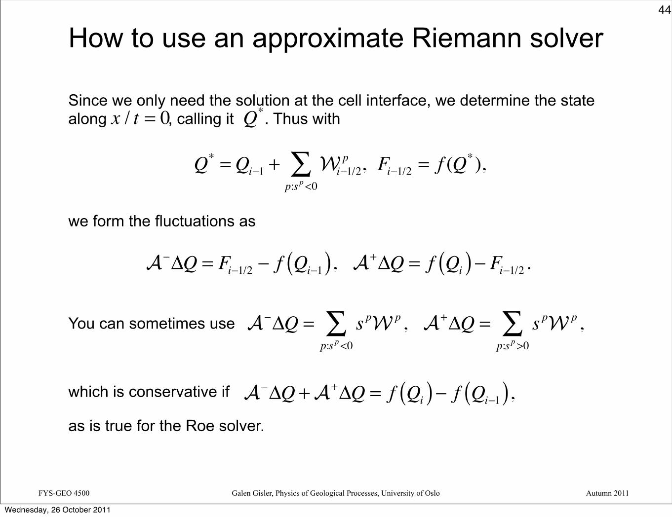
How to use an approximate Riemann solver
Since we only need the solution at the cell interface, we determine the state along , calling it . Thus with
we form the fluctuations as
You can sometimes use
which is conservative if
as is true for the Roe solver.
x / t = 0 Q*
Q* =Qi−1 + Wi−1/2p
p:s p<0∑ , Fi−1/2 = f (Q*),
A−ΔQ = Fi−1/2 − f Qi−1( ), A+ΔQ = f Qi( )− Fi−1/2 .
A−ΔQ = s pW p
p:s p<0∑ , A+ΔQ = s pW p
p:s p>0∑ ,
A−ΔQ +A+ΔQ = f Qi( )− f Qi−1( ),
44
Wednesday, 26 October 2011

FYS-GEO 4500 Galen Gisler, Physics of Geological Processes, University of Oslo Autumn 2011
Example: Roe solver for shallow-water equations
= depth
= bulk speed, varies only with x
Conservation of mass and momentum gives the system:
which has the Jacobian matrix:
qt + f (q)x =hhu
⎡
⎣⎢
⎤
⎦⎥t
+hu
hu2 + 12gh2
⎡
⎣
⎢⎢⎢
⎤
⎦
⎥⎥⎥x
= 0.
′f (q) =0 1
−u2 + gh 2u⎡
⎣⎢⎢
⎤
⎦⎥⎥, λ=u ± gh.
h = height of wave above bottom
u = speed of bulk water motionρ = water density
h(x,t)u(x,t)
45
Wednesday, 26 October 2011

FYS-GEO 4500 Galen Gisler, Physics of Geological Processes, University of Oslo Autumn 2011
Roe solver for Shallow Water
Given define .
Then if is defined as the Jacobian matrix evaluated at the special state
we find that:
the Roe conditions are satisfied,
an isolated shock is modelled well,
and the wave propagation algorithm is conservative.
If we use limited waves, we obtain high-resolution methods as before.
hl ,ul ,hr ,ur , h = hl + hr2
, u =hl ul + hrurhl + hr
Aq = (h ,hu),
46
Wednesday, 26 October 2011

FYS-GEO 4500 Galen Gisler, Physics of Geological Processes, University of Oslo Autumn 2011
Roe solver for Shallow Water
Given define .
Then if is defined as the Jacobian matrix evaluated at the special state
we find that:
the Roe conditions are satisfied,
an isolated shock is modelled well,
and the wave propagation algorithm is conservative.
If we use limited waves, we obtain high-resolution methods as before.
hl ,ul ,hr ,ur , h = hl + hr2
, u =hl ul + hrurhl + hr
Aq = (h ,hu),
“Roe average”
46
Wednesday, 26 October 2011
FYS-GEO 4500 Galen Gisler, Physics of Geological Processes, University of Oslo Autumn 2011
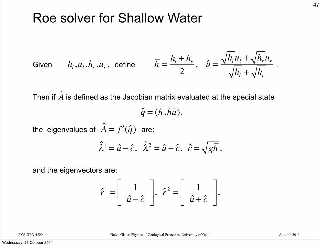
Roe solver for Shallow Water
Given define .
Then if is defined as the Jacobian matrix evaluated at the special state
the eigenvalues of are:
and the eigenvectors are:
hl ,ul ,hr ,ur , h = hl + hr2
, u =hl ul + hrurhl + hr
A = ′f (q)
λ1 = u − c, λ2 = u − c, c = gh ,
r1 = 1u − c
⎡
⎣⎢
⎤
⎦⎥, r 2 = 1
u + c⎡
⎣⎢
⎤
⎦⎥,
Aq = (h ,hu),
47
Wednesday, 26 October 2011

FYS-GEO 4500 Galen Gisler, Physics of Geological Processes, University of Oslo Autumn 2011
The Shallow-water Riemann solver in Clawpack is a Roe solver
“Roe average”
from: $CLAW/book/chap13/swhump1/rp1sw.f
h = hl + hr2
, u =hl ul + hrurhl + hr
48
Wednesday, 26 October 2011

FYS-GEO 4500 Galen Gisler, Physics of Geological Processes, University of Oslo Autumn 2011
Roe solver for the Euler equationsThe eigensystem of the Euler equations for a polytropic gas is:
These need to be evaluated at the Roe-averaged state, so we need the Roe averages for u, H, c. These are:
λ1 = u − c λ2 = u λ 3 = u + c
r1 =1
u − cH − uc
⎡
⎣
⎢⎢⎢
⎤
⎦
⎥⎥⎥
r2 =1u12 u
2
⎡
⎣
⎢⎢⎢
⎤
⎦
⎥⎥⎥
r3 =1
u + cH + uc
⎡
⎣
⎢⎢⎢
⎤
⎦
⎥⎥⎥
u =ρi−1ui−1 + ρi uiρi−1 + ρi
H =ρi−1Hi−1 + ρi Hi
ρi−1 + ρi
c = γ −1( ) H − 12u2⎛
⎝⎜⎞⎠⎟
49
Wednesday, 26 October 2011

FYS-GEO 4500 Galen Gisler, Physics of Geological Processes, University of Oslo Autumn 2011
Roe solver for the Euler equations
Then the wave decomposition between the left and right states is
where Qi
nQi−1n
Riemann
Roe
δ ≡Qi −Qi−1 = α1r1 +α 2r 2 +α 3r 3
QinQi−1
n
α 2 = γ −1( )H − u2( )δ 1 + uδ 2 −δ 3
c2
α 3 =δ 2 + c − u( )δ 1 − cα 2
2cα1 = δ 1 −α 2 −α 3
But note that, while the Riemann solution consists of three waves, one of which is a rarefaction fan, the Roe solution only consists of three waves. In most cases this does not matter, since the desired solution at x/t=0 will be the same intermediate state. In the case of a transonic rarefaction a modification (in the form of an entropy fix) is necessary.
50
Wednesday, 26 October 2011

FYS-GEO 4500 Galen Gisler, Physics of Geological Processes, University of Oslo Autumn 2011
Entropy fix for transonic rarefactions
Suppose there is a transonic rarefaction in the k wave:
The method proposed by Harten and Hyman, modified slightly by Leveque, and implemented in Clawpack, is the following. Define
where is the Roe-averaged eigenvalue for this wave. Then in computing the fluctuations
for the speed of the k wave use
λlk < 0 < λr
k , qlk =Qi−1 + W p , qrk = qlk +
p=1
k−1
∑ W k
λk
β = λkr − λk
λkr − λ l
k
A−ΔQi−1/2 = si−1/2
p( )−Wi−1/2p
p∑ , A+ΔQi−1/2 = si−1/2
p( )+Wi−1/2p
p∑
λ k( )− = βλlk , λ k( )+ = 1− β( )λrk
51
Wednesday, 26 October 2011

FYS-GEO 4500 Galen Gisler, Physics of Geological Processes, University of Oslo Autumn 2011
The Harten-Lax-van Leer (HLL) Solver
This solver uses only 2 waves with s1 = minimum characteristic speeds2 = maximum characteristic speed
Write
where the middle state is uniquely determined by the conservation requirement:
Modifications of this include positivity constraints and the addition of a third wave.
W1 =Q* − ql , W 2 = qr −Q*
Q*
s1W1 + s2W 2 = f (qr )− f (ql )
⇒Q* = f (qr )− f (ql )− s2qr + s
1qls1 − s2
52
Wednesday, 26 October 2011

FYS-GEO 4500 Galen Gisler, Physics of Geological Processes, University of Oslo Autumn 2011
Riemann solvers: exact vs approximate?
Whether to use a Roe solver, or other approximate Riemann solver, as opposed to an iterative exact solver is debatable.
Exact solvers are typically costly in time and storage
You don’t need all the information generated
However, if you use a Roe solver:
You don’t get the full structure of the rarefaction wave
In certain circumstances, the approximation may be poor
As computers and methods improve, more people may prefer exact iterative solvers.
53
Wednesday, 26 October 2011

FYS-GEO 4500 Galen Gisler, Physics of Geological Processes, University of Oslo Autumn 2011
How good is the Roe solver?
Example for the Euler equations, comparing iterative exact and approximate Roe solvers.
When the left and right states are close together, the Roe solver is very good.
0.2900
0.2975
0.3050
0.3125
0.3200
0.490 0.495 0.500 0.505 0.510
u
p
0.2900
0.2975
0.3050
0.3125
0.3200
0.9900 0.9975 1.0050 1.0125 1.0200
u
rho
Roe solverExact RiemannRoe average
Left State
Right State
Roe Average
Qin
xi−1/2Qi−1
n
ql
ql* qr
*
qr
54
Solved Intermediate States
Wednesday, 26 October 2011

FYS-GEO 4500 Galen Gisler, Physics of Geological Processes, University of Oslo Autumn 2011
0
0.5
1.0
1.5
2.0
0 1 2 3 4
u
p
0
0.5
1.0
1.5
2.0
0 1 2 3 4
u
rho
Roe solverExact RiemannRoe average
How good is the Roe solver?
When the left and right states are connected by a single shock, there are no intermediate states, and the Roe solver is exact
Left State
Roe Average
Right State
Qin
xi−1/2Qi−1
n
ql qr
55
Wednesday, 26 October 2011

FYS-GEO 4500 Galen Gisler, Physics of Geological Processes, University of Oslo Autumn 2011
0
0.5
1.0
1.5
2.0
0 1 2 3 4
u
p
0
0.5
1.0
1.5
2.0
0 0.75 1.50 2.25 3.00
u
rho
Roe solverExact RiemannRoe average
How good is the Roe solver?
For arbitrary right and left states, the Roe solver is definitely inaccurate.
If the resolution is sufficiently good, this circumstance should not occur in practice.
But in the other two cases, one or two iterations in the exact solve may be enough.
Left State
Right State
Roe Average
Qin
xi−1/2Qi−1
n
ql
ql* qr
*
qr
56
Solved Intermediate States
Wednesday, 26 October 2011

FYS-GEO 4500 Galen Gisler, Physics of Geological Processes, University of Oslo Autumn 2011
f-wave approximate Riemann solver
Instead of splitting Q into waves, we might consider splitting the flux f into “waves” :
It turns out this is useful for spatially varying flux functions, i.e.
with applications, for example, in:
wave propagation in heterogeneous nonlinear media,
flow in heterogeneous porous media,
traffic flow with varying road conditions,
conservation laws on curved manifolds,
and certain kinds of source terms.
f (Qi )− f (Qi−1) = Zi−1/2p
p=1
Mw
∑(Mw ≤ w)
Mw
qt + f (q, x)x = 0,
57
Wednesday, 26 October 2011

FYS-GEO 4500 Galen Gisler, Physics of Geological Processes, University of Oslo Autumn 2011
Flux-based wave decomposition (f-waves)
Choose wave forms rp (for example, eigenvectors of the Jacobian on each side).
Then decompose the flux difference:
fr (qr )− fl (ql ) = β pr p
p=1
m
∑ = Z pp=1
m
∑
qr
W2 W
3
ql
W1
qr*ql
*
ql + fl (q)x = 0 qr + fr (q)x = 0
58
Wednesday, 26 October 2011

FYS-GEO 4500 Galen Gisler, Physics of Geological Processes, University of Oslo Autumn 2011
Wave propagation algorithm using waves
In the standard version:
Qi
n+1 =Qin − Δt
ΔxA−ΔQi+1/2 +A+ΔQi−1/2( )− Δt
ΔxFi+1/2 − Fi−1/2( )
Qi −Qi−1 = Wi−1/2p
p=1
m
∑
A−ΔQi+1/2 = si+1/2p( )−Wi+1/2p
p∑
A+ΔQi−1/2 = si−1/2p( )+Wi−1/2p
p∑
Fi−1/2 =12
si−1/2p 1− Δt
Δxsi−1/2p⎛
⎝⎜⎞⎠⎟Wi−1/2p
p=1
m
∑
⎧
⎨
⎪⎪⎪⎪⎪
⎩
⎪⎪⎪⎪⎪
59
Wednesday, 26 October 2011

FYS-GEO 4500 Galen Gisler, Physics of Geological Processes, University of Oslo Autumn 2011
Wave propagation algorithm using f-waves
Using f-waves:
Qi
n+1 =Qin − Δt
ΔxA−ΔQi+1/2 +A+ΔQi−1/2( )− Δt
ΔxFi+1/2 − Fi−1/2( )
fi (Qi )− fi−1(Qi−1) = Zi−1/2p
p=1
m
∑A−ΔQi+1/2 = Zi+1/2p
p:si−1/2p <0∑A+ΔQi−1/2 = Zi−1/2p
p:si−1/2p >0∑
Fi−1/2 =12
sgn si−1/2p( ) 1− Δt
Δxsi−1/2p⎛
⎝⎜⎞⎠⎟Zi−1/2p
p=1
m
∑
⎧
⎨
⎪⎪⎪⎪⎪
⎩
⎪⎪⎪⎪⎪
60
Wednesday, 26 October 2011

FYS-GEO 4500 Galen Gisler, Physics of Geological Processes, University of Oslo Autumn 2011
f-wave approximate Riemann solver
Let be any averaged Jacobian matrix, for example:
Use eigenvectors of to do f-wave splitting.
Then , so the method is conservative.
If is the Roe average, then this is equivalent to the normal Roe Riemann solver, and
A
A = ′f ql + qr2
⎛⎝⎜
⎞⎠⎟
A−ΔQi+1/2 +A+ΔQi−1/2 = f (Qi )− f (Qi−1)
A
A Z
p = s pW p .
61
Wednesday, 26 October 2011

FYS-GEO 4500 Galen Gisler, Physics of Geological Processes, University of Oslo Autumn 2011
Assignment for next time
Read Chapter 14 and Chapter 15.
Write (in Fortran or Python) an approximate Riemann solver for the Euler equations using the Roe average. Test it on the shock tube problem, or (optionally) on the Woodward-Colella blast-wave problem. Use the shallow-water Riemann solver as a guide.
62
Wednesday, 26 October 2011