fuzzy continuous classification and spatial interpolation in conventional soil survey for soil...

www.elsevier.com/locate/geoderma

Geoderma 118 (2004) 1–16

Fuzzy continuous classification and spatial interpolation in

conventional soil survey for soil mapping of the lower Piave plain

Gilberto Bragato*

Istituto Sperimentale per la Nutrizione delle Piante, Section of Gorizia, Via Trieste 23, I-34170 Gorizia, Italy

Received 13 November 2002; accepted 28 March 2003

Abstract

Soil maps on a reconnaissance or semi-detailed scale are frequently used as the basic level of information for regional land

use assessment. However, they are impractical for suitability predictions concerning quality crops, which require an

enlargement of details that can be guaranteed only by detailed soil survey and mapping. The change of scale increases the

importance of field observations and introduces in the soil-landscape model the fuzziness related to surveyor’s subjective

judgement. The present study explored the applicability of the fuzzy c-means approach to conventional soil surveys for detailed

land use assessment with the purpose of taking into consideration the fuzziness of data collected in areas where soil type

transitions are not easily observable on the surface. The investigation was done using data from 1888 auger borings of a 42000-

ha survey carried out in the lower part of the fluvial plain east of Venice on the 1:25000 map scale. The morphological

quantitative attributes of the master horizons A, Bw, Bg, Bk and C were first reduced in number so as to remove attribute

redundancy. They were then submitted to fuzzy c-means, testing cluster validity with both internal and external criterion

measures. The best partition was obtained with four classes, which were consistent with the main soil-forming processes of the

area not only in terms of class centre features, but also of spatial variability and distribution pattern of the class memberships.

The investigated approach might represent part of a complex analytical sequence capable of using both the spatial distribution

of fuzzy continuous classes and the landform analysis to formulate a spatially detailed territorial model representing the basic

level of information for a locally oriented land use assessment.

D 2003 Elsevier Science B.V. All rights reserved.

Keywords: Augering data; Compositional kriging; Continuous soil map; Fuzzy sets; Fuzzy clustering; Soil survey

1. Introduction

The development of soil studies has been strongly

influenced not only by the progress of scientific

knowledge, but also by land use planning that, along

with the large amount of information acquired by

national soil bureaux, increased the emphasis given

0016-7061/$ - see front matter D 2003 Elsevier Science B.V. All rights re

doi:10.1016/S0016-7061(03)00166-6

* Fax: +39-0481-520208.

E-mail address: [email protected] (G. Bragato).

by land evaluation methodologies to the soil resource

(Rossiter, 1996). Land use assessment has devoted

much of its interest to reconnaissance or semi-detailed

soil maps that are effective in planning the use of land

in a region. However, more detailed land use predic-

tions and maps are required in areas where quality

crops are grown (see Costantini et al., 1996; Lebon et

al., 1997 for grapevine production) and the quality of

the product is affected by environmental, locally

variable factors which relationship with quality pro-

served.

G. Bragato / Geoderma 118 (2004) 1–162

ductions sometimes derived from a century-old local

selection.

This change of scale does not merely require an

enlargement of details, but involves a substantial

methodological change in the mapping practice, and

often needs new surveys for a thorough updating of

existing soil information. The increase of detail

strongly increases both the importance of the soil-

landscape model originating from Jenny’s (1941)

equation and the weight of field observations as

opposed to aerial photographs and remote sensing.

According to the soil-landscape model, there is a close

relationship between the landform pattern and the

geographical distribution of soil types, allowing sur-

veyors to differentiate soil mapping units whenever

lateral short-distance discontinuities of observable

surface features are found (Hudson, 1992). The model

assumptions generate a discrete picture of the soil

pattern, where soil units are delimited with sharp,

rigidly defined boundaries. In fact soil spatial distri-

bution fluctuates between a discontinuous and a con-

tinuous model because the physiographic discontinu-

ities and the gradual subsurface variation across

boundaries and within soil units are not marked. The

discrepancy between the discrete model and the actual

soil distribution produces an indeterminacy that

increases while deviating from model assumptions

(Lagacherie et al., 1996). Indeterminacy derives both

from the lack of knowledge on the pattern of soil

distribution, and from the vagueness—or fuzziness—

related to the intrinsic imprecision of the human

reasoning while experiencing and interpreting the

complexity of the real world (Sangalli, 1998). The

lack of knowledge is the main aspect the surveyor tries

to minimize when dealing with map delineation accu-

racy. The second aspect—the fuzziness—is introduced

in the soil-landscape model through the tacit knowl-

edge (Hudson, 1992) achieved in the field during the

auger borings campaign and it is used to delineate soil

units and to locate representative profiles.

Auger borings are described in terms of quantita-

tive and qualitative morphological features based on

the surveyor’s subjective judgement. The surveyor

writes down a large, hardly manageable amount of

information—concerning subsurface features in par-

ticular—that is normally underused in the next steps

of the survey. Both the fuzziness and the amount of

field observations may be processed with the multi-

valued approach of fuzzy sets that, assuming the

partial rather than the full membership of an individ-

ual to a set of objects, can handle a subjective

judgement better than the usual Boolean approach

(Zimmerman, 1996). When soil information is

updated to increase the detail of a soil map, one of

the most suitable methods of data analysis is the non-

hierarchical multivariate approach of fuzzy c-means

(FCM) (Bezdek, 1981), a generalization of the hard k-

means clustering also known as fuzzy k-means. Its

usefulness for soil science was debated by McBratney

and de Gruijter (1992) and McBratney et al. (1992).

Although FCM has been already used in soil

classification (Mazaheri et al., 1995) and mapping

(Odeh et al., 1992; de Gruijter et al., 1997; Lagacherie

et al., 1997), data and sampling densities comparable

to those of detailed soil surveys have been used in

very few studies. Morphological properties usually

observed in soil surveys were processed by Verheyen

et al. (2001). They first splitted field-observed hori-

zons into more homogeneous horizons subtypes using

ordination methods. Auger borings were then de-

scribed in terms of presence and thickness of the

horizon subtypes and submitted to FCM. However,

part of the fuzziness of observations could have been

lost at the end of the clustering procedure. Further-

more, the surveyed area was too small and the density

of observations too large to be compared to the

working practice of detailed surveys. A more realistic

density was adopted by Triantafilis et al. (2001),

whose procedure retained much of the gradation

between soil types. This notwithstanding, they made

observations at fixed depths and considered soil

attributes that are usually not determined on auger

borings. A data set from a really conventional detailed

survey was used by Carre and Girard (2002). These

authors tested a dynamic fuzzy clustering procedure

that allowed them to identify centroidal horizon and

soil types, and to measure the taxonomic distance

between soil individuals and centroidal soil types.

Contrary to the FCM approach of Triantafilis et al.

(2001), they based their procedure on the conceptual

framework of an existing classification system—the

Referentiel Pedologique (Baize and Girard, 1995)—

and of its elementary units—the reference horizons—

from which they derived the concept of centroidal

horizon types. Moreover, they interpolated taxonomic

distances at unsampled locations using a multiple

G. Bragato / Geoderma 118 (2004) 1–16 3

linear regression of intensively observed covariates

coming from terrain and land cover information rather

than directly analysing the spatial variability of taxo-

nomic distances, and interpolating them with kri-

ging.The present study took origin from the idea of

de Bruin and Stein (1998) that the ‘‘incorporation of

full soil profile data would improve the utility of fuzzy

c-means clustering for soil-landscape modelling’’. It

has been addressed to the applicability of FCM to

conventional detailed surveys for land use assessment

in areas characterized by gradual soil type transitions

not easily observable on the surface. The specific

purpose of the study was to find out a procedure that,

without starting from any existing classification,

would be capable of: (i) emphasizing the main soil

forming processes behind the collected data; (ii)

considering and representing gradual soil type tran-

sitions; and, (iii) producing fuzzy continuous maps for

a first delineation of soil mapping units.

2. Materials and methods

2.1. Study area and data set

The fuzzy continuous classification approach to

conventional survey was tested in a 42000-ha fluvial

plain portion east of Venice. The study area is in the

lower part of the River Piave plain at an elevation

ranging from +6 to �2 mas l. The river is responsible

for the formation of the central and northern part of

the Venice lagoon. Since the Wurm glacial period, the

alluvial landscape has been strongly influenced by the

gradual translation of the Piave from west to east. In

the last centuries, the landscape was also affected by

the deviation of the river carried out by the Venetians

in the 17th century in order to stop city floods and the

filling of the lagoon. After the 17th century, part of the

area was periodically flooded until soils were

reclaimed for agriculture at the beginning of the

20th century. The investigated area and its present

and past hydrography are summarized in Fig. 1. The

area is delimited by the River Sile to the west and the

River Livenza to the east. The former was deviated

from the Venice lagoon to the ancient Piave riverbed

that now marks the eastern boundary of the lagoon.

The alluvial deposits took origin from the dolomitic

limestones of the upper river basin. They are orga-

nized in strata of varying textural composition due to

the alternating climatic changes of the Wurm period

and the frequent variations of the sea level since then.

The high calcium carbonate content and the frequency

of floods are responsible for the limited soil evolution,

with soil typology roughly ranging from young Flu-

visols to old Calcisols (FAO-UNESCO, 1994).

The data set consists of 1888 auger borings located

through a purposive sampling strategy and made to a

maximum depth of 120 cm. The data were recorded

following the prescriptions of the ISSDS manual

(Istituto Sperimentale per lo Studio e la Difesa del

Suolo, 1995). The soil survey was carried out between

1995 and 1997 to produce a soil map on a scale of

1:25000. Part of the map, along with a grapevine

suitability evaluation, was published in 1996 (Ente di

Sviluppo Agricolo del Veneto, 1996a). Table 1 reports

the most representative soil types according to FAO-

UNESCO (1994) and USDA (Soil Survey Staff,

1994) classification.

2.2. Attribute selection

Soil profiles usually show two to five horizons

between 0 and 120 cm, and each horizon can be

described in terms of the following standard set of

attributes: thickness; matrix colour; colour, size, area

percentage of low and high-chroma mottles; hand-

estimated texture of the fine earth fraction; type, size

and volume percentage of rock fragments; type, size

and volume percentage of concentrations; efferves-

cence; pH.

Given these characteristics, the relationships be-

tween horizons, and the surveyor’s observations on

the field, horizons are described while inferring the

prevailing soil-forming processes which took place in

the site. Not all standard attributes are actually ob-

served in each horizon, and in detailed surveys some

of them remain often undetected all over the investi-

gated area. The auger boring of Table 2, for instance,

has three horizons (A, Bw and BC) with 5, 10 and 12

attributes, respectively. This soil individual, being

characterized by eight qualitative (colours and effer-

vescence) and 19 quantitative attributes, looks quite

simple compared to the samples where more than 40

quantitative attributes per auger boring are detected.

Such a large number of attributes in the data set would

be difficult to process using any multivariate analysis

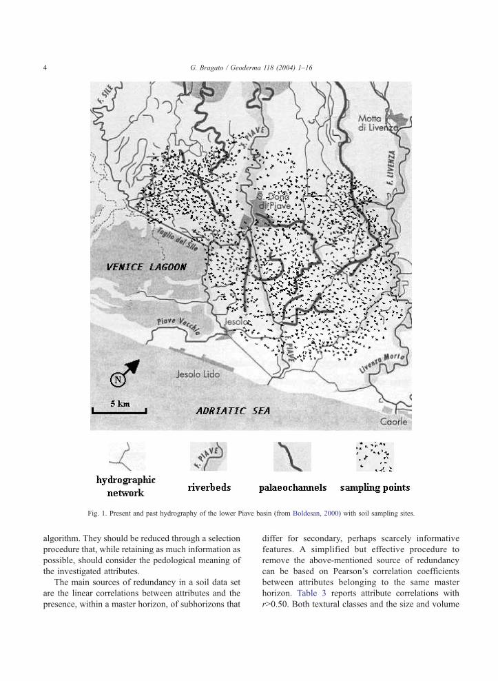
Fig. 1. Present and past hydrography of the lower Piave basin (from Boldesan, 2000) with soil sampling sites.


algorithm. They should be reduced through a selection

procedure that, while retaining as much information as

possible, should consider the pedological meaning of

the investigated attributes.

The main sources of redundancy in a soil data set

are the linear correlations between attributes and the

presence, within a master horizon, of subhorizons that

differ for secondary, perhaps scarcely informative

features. A simplified but effective procedure to

remove the above-mentioned source of redundancy

can be based on Pearson’s correlation coefficients

between attributes belonging to the same master

horizon. Table 3 reports attribute correlations with

r>0.50. Both textural classes and the size and volume

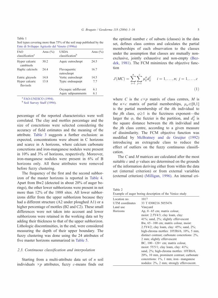
Table 1

Soil types covering more than 75% of the soil map published by the

Ente di Sviluppo Agricolo del Veneto (1996a)

FAO

classificationaArea (%) USDA

classificationbArea (%)

Hyper calcaric

cambisols

30.2 Aquic eutrochrept 24.5

Haplic calcisols 24.4 Fluvaquentic

eutrochrept

16.7

Eutric gleysols 14.8 Vertic eutrochrept 14.5

Hyper calcaric

fluvisols

13.8 Typic endoaquept 7.7

Oxyaquic udifluvent 6.1

Aquic udipsamments 6.1

a FAO-UNESCO (1994).b Soil Survey Staff (1994).

Table 2

Example of auger boring description of the Venice study

Location no. 1017

UTM coordinates 33 T 0300216 5055476

Land use Vineyard

Horizons Ap, 0–65 cm; matrix colour,

moist: 2.5Y4/3; clay loam, clay:

41%; sand, 2%; slightly effervescent

Bw, 65–100 cm; matrix colour, moist:

2.5Y4/2; clay loam, clay: 45%; sand, 2%;

high-chroma mottles: 10YR6/6, 10%, 5 mm,

distinct contrast; carbonate concretions: 2%,

2 mm; slightly effervescent

BC, 100–120+ cm; matrix colour,

moist: 5Y5/1; clay loam, clay: 41%;

sand, 2%; high-chroma mottles: 10YR6/6,

20%, 10 mm, prominent contrast; carbonate

concretions: 1%, 1 mm; iron–manganese

nodules: 2%, 2 mm; strongly effervescent.


percentage of the reported characteristics were well

correlated. The clay and mottles percentage and the

size of concretions were selected considering the

accuracy of field estimates and the meaning of the

attribute. Table 3 suggests a further exclusion: as

expected, concentrations were absent in C horizons

and scarce in A horizons, where calcium carbonate

concretions and iron-manganese nodules were present

in 10% and 3% of horizons, respectively. Moreover,

iron-manganese nodules were present in 6% of B

horizons only. All these attributes were removed

before fuzzy clustering.

The frequency of the first and the second subhor-

izon of the master horizons is reported in Table 4.

Apart from Bw2 (detected in about 20% of auger bo-

rings), the other lower subhorizons were present in not

more than 12% of the 1888 sites. All lower subhor-

izons differ from the upper subhorizon because they

had a different structure (A2 under ploughed A1) or a

higher percentage of mottles (B2 and C2). These small

differences were not taken into account and lower

subhorizons were retained in the working data set by

adding their thickness to that of the upper subhorizon.

Lithologic discontinuities, in the end, were considered

measuring the depth of their upper boundary. The

fuzzy clustering was done using the 24 attributes of

five master horizons summarized in Table 5.

2.3. Continuous classification and interpolation

Starting from a multi-attribute data set of n soil

individuals �p attributes, fuzzy c-means finds out

the optimal number c of subsets (classes) in the data

set, defines class centres and calculates the partial

memberships of each observation to the classes

under the assumption that classes are mutually non-

exclusive, jointly exhaustive and non-empty (Bez-

dek, 1981). The FCM minimizes the objective func-

tion

JðMCÞ ¼Xn

i¼1

Xc

j¼1

luij d

2ij i ¼ 1; . . . ; n; j ¼ 1; . . . ; c

ð1Þ

where C is the c�p matrix of class centres, M is

the n�c matrix of partial memberships, lica[0,1]

is the partial membership of the ith individual to

the jth class, uz1 is the fuzziness exponent—the

larger the u, the fuzzier is the partition, and dij2 is

the square distance between the ith individual and

the jth class centre, according to a given measure

of dissimilarity. The FCM objective function was

modified by McBratney and de Gruijter (1992)

introducing an extragrade class to reduce the

effect of outliers on the fuzzy continuous classifi-

cation.

The C and M matrices are calculated after the most

suitable c and u values are determined on the grounds

of the information deriving either from within the data

set (internal criterion) or from external variables

(external criterion) (Milligan, 1996). An internal cri-

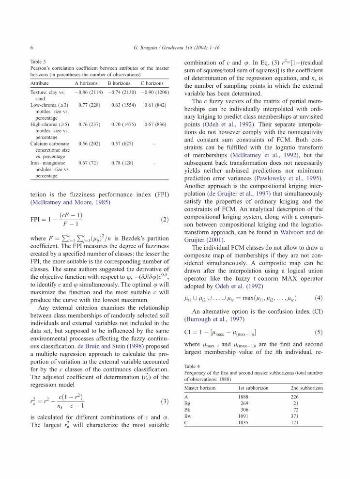
Table 3

Pearson’s correlation coefficient between attributes of the master

horizons (in parentheses the number of observations)

Attribute A horizons B horizons C horizons

Texture: clay vs.

sand

�0.86 (2114) �0.74 (2130) �0.90 (1206)

Low-chroma (V3)

mottles: size vs.

percentage

0.77 (228) 0.63 (1554) 0.61 (842)

High-chroma (z5)

mottles: size vs.

percentage

0.76 (237) 0.70 (1475) 0.67 (836)

Calcium carbonate

concretions: size

vs. percentage

0.56 (202) 0.57 (627) –

Iron–manganese

nodules: size vs.

percentage

0.67 (72) 0.78 (128) –

Table 4

Frequency of the first and second master subhorizons (total number

of observations: 1888)

Master horizon 1st subhorizon 2nd subhorizon

A 1888 226

Bg 269 21

Bk 306 72

Bw 1091 371

C 1035 171


terion is the fuzziness performance index (FPI)

(McBratney and Moore, 1985)

FPI ¼ 1� ðcF � 1ÞF � 1

ð2Þ

where F ¼Pn

i¼1

Pcj¼1ðlijÞ2=n is Bezdek’s partition

coefficient. The FPI measures the degree of fuzziness

created by a specified number of classes: the lesser the

FPI, the more suitable is the corresponding number of

classes. The same authors suggested the derivative of

the objective function with respect to u, �(dJ/du)c0.5,to identify c and u simultaneously. The optimal u will

maximize the function and the most suitable c will

produce the curve with the lowest maximum.

Any external criterion examines the relationship

between class memberships of randomly selected soil

individuals and external variables not included in the

data set, but supposed to be influenced by the same

environmental processes affecting the fuzzy continu-

ous classification. de Bruin and Stein (1998) proposed

a multiple regression approach to calculate the pro-

portion of variation in the external variable accounted

for by the c classes of the continuous classification.

The adjusted coefficient of determination (ra2) of the

regression model

r2a ¼ r2 � cð1� r2Þns � c� 1

ð3Þ

is calculated for different combinations of c and u.The largest ra

2 will characterize the most suitable

combination of c and u. In Eq. (3) r2=[1�(residual

sum of squares/total sum of squares)] is the coefficient

of determination of the regression equation, and ns is

the number of sampling points in which the external

variable has been determined.

The c fuzzy vectors of the matrix of partial mem-

berships can be individually interpolated with ordi-

nary kriging to predict class memberships at unvisited

points (Odeh et al., 1992). Their separate interpola-

tions do not however comply with the nonnegativity

and constant sum constraints of FCM. Both con-

straints can be fulfilled with the logratio transform

of memberships (McBratney et al., 1992), but the

subsequent back transformation does not necessarily

yields neither unbiased predictions nor minimum

prediction error variances (Pawlowsky et al., 1995).

Another approach is the compositional kriging inter-

polation (de Gruijter et al., 1997) that simultaneously

satisfy the properties of ordinary kriging and the

constraints of FCM. An analytical description of the

compositional kriging system, along with a compari-

son between compositional kriging and the logratio-

transform approach, can be found in Walvoort and de

Gruijter (2001).

The individual FCM classes do not allow to draw a

composite map of memberships if they are not con-

sidered simultaneously. A composite map can be

drawn after the interpolation using a logical union

operator like the fuzzy t-conorm MAX operator

adopted by Odeh et al. (1992)

li1 [ li2 [ . . . [ lic ¼ maxðli1; li2; . . . ; licÞ ð4Þ

An alternative option is the confusion index (CI)

(Burrough et al., 1997)

CI ¼ 1� ½lmaxi � lðmax�1Þi� ð5Þ

where lmax i and l(max�1)i are the first and second

largest membership value of the ith individual, re-

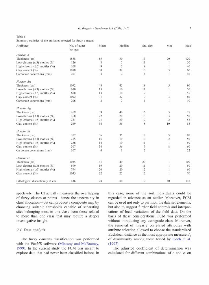
Table 5

Summary statistics of the attributes selected for fuzzy c-means

Attributes No. of auger

borings

Mean Median Std. dev. Min Max

Horizon A

Thickness (cm) 1888 55 50 13 20 120

Low-chroma (V3) mottles (%) 126 8 5 11 1 50

High-chroma (z5) mottles (%) 108 9 5 9 1 40

Clay content (%) 1888 30 32 10 3 60

Carbonate concretions (mm) 201 3 2 4 1 40

Horizon Bw

Thickness (cm) 1092 48 45 19 5 90



Clay content (%) 1092 31 32 9 3 60


Horizon Bg

Thickness (cm) 269 39 40 16 5 75



Clay content (%) 269 34 36 8 10 55

Horizon Bk

Thickness (cm) 307 36 35 18 5 80



Clay content (%) 307 34 36 9 8 60


Horizon C

Thickness (cm) 1035 41 40 20 1 100



Clay content (%) 1035 22 25 13 1 70

Lithological discontinuity at cm 436 78 80 19 40 118


spectively. The CI actually measures the overlapping

of fuzzy classes at points—hence the uncertainty in

class allocation—but can produce a composite map by

choosing suitable thresholds capable of separating

sites belonging most to one class from those related

to more than one class that may require a deeper

investigative insight.

2.4. Data analysis

The fuzzy c-means classification was performed

with the FuzME software (Minasny and McBratney,

1999). In the current study the FCM was meant to

explore data that had never been classified before. In

this case, none of the soil individuals could be

regarded in advance as an outlier. Moreover, FCM

can be used not only to partition the data set elements,

but also to suggest further field controls and interpre-

tations of local variations of the field data. On the

basis of these considerations, FCM was performed

without introducing any extragrade class. Moreover,

the removal of linearly correlated attributes with

attribute selection allowed to choose the standardized

Euclidean distance as the most appropriate measure dijof dissimilarity among those tested by Odeh et al.

(1992).

The adjusted coefficient of determination was

calculated for different combinations of c and u on


a subset of 50 surveyed sites randomly selected in the

data set and resampled in the 0–30 cm soil layer. In

the laboratory, samples were air-dried, sieved at 2.00

mm and dispersed in a sodium hexametaphosphate

solution. Their sand content (0.05–2.00 mm) was

measured with the pipette method (Ministero per le

Politiche Agricole e Forestali, 2000). The sand con-

tent was chosen because (i) its field estimates had

been excluded from the working data set; (ii) its

laboratory determination is fast and simple; and, (iii)

the fluvial sedimentation affects its topsoil variation in

space.

The spatial variability of fuzzy memberships

were investigated using variogram analysis proce-

dure of the ISATIS 3.3 geostatistical package (Geo-

variances, 2000). The fuzzy membership classes

were mapped after compositional kriging interpola-

tion (de Gruijter et al., 1997), and interpolated

partial memberships were post-processed to produce

the compositional maps of MAX memberships and

CI.

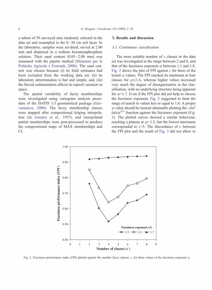
Fig. 2. Fuzziness performance index (FPI) plotted against the numbe

3. Results and discussion

3.1. Continuous classification

The most suitable number of c classes in the data

set was investigated in the range between 2 and 8, and

that of the fuzziness exponent u between 1.1 and 1.8.

Fig. 2 shows the plot of FPI against c for three of the

tested u values. The FPI reached its minimum at four

classes for uV1.6, whereas higher values increased

very much the degree of disorganisation in the clas-

sification, with no underlying structure being apparent

for u=1.7. Even if the FPI plot did not help to choose

the fuzziness exponent, Fig. 2 suggested to limit the

range of search to values less or equal to 1.6. A proper

u value should be instead obtainable plotting the�(yJ/ydu)c0.5 function against the fuzziness exponent (Fig.

3). The plotted curves showed a similar behaviour,

reaching a plateau at u=1.5, but the lowest maximum

corresponded to c=3. The discordance of c between

the FPI plot and the result of Fig. 3 did not allow to

r fuzzy classes, c, for three values of the fuzziness exponent u.

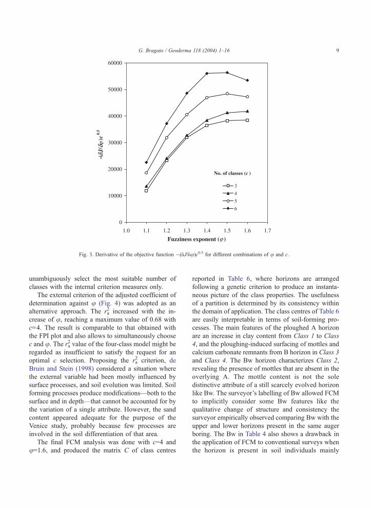
Fig. 3. Derivative of the objective function �(yJ/yu)c0.5 for different combinations of u and c.


unambiguously select the most suitable number of

classes with the internal criterion measures only.

The external criterion of the adjusted coefficient of

determination against u (Fig. 4) was adopted as an

alternative approach. The ra2 increased with the in-

crease of u, reaching a maximum value of 0.68 with

c=4. The result is comparable to that obtained with

the FPI plot and also allows to simultaneously choose

c and u. The ra2 value of the four-class model might be

regarded as insufficient to satisfy the request for an

optimal c selection. Proposing the ra2 criterion, de

Bruin and Stein (1998) considered a situation where

the external variable had been mostly influenced by

surface processes, and soil evolution was limited. Soil

forming processes produce modifications—both to the

surface and in depth—that cannot be accounted for by

the variation of a single attribute. However, the sand

content appeared adequate for the purpose of the

Venice study, probably because few processes are

involved in the soil differentiation of that area.

The final FCM analysis was done with c=4 and

u=1.6, and produced the matrix C of class centres

reported in Table 6, where horizons are arranged

following a genetic criterion to produce an instanta-

neous picture of the class properties. The usefulness

of a partition is determined by its consistency within

the domain of application. The class centres of Table 6

are easily interpretable in terms of soil-forming pro-

cesses. The main features of the ploughed A horizon

are an increase in clay content from Class 1 to Class

4, and the ploughing-induced surfacing of mottles and

calcium carbonate remnants from B horizon in Class 3

and Class 4. The Bw horizon characterizes Class 2,

revealing the presence of mottles that are absent in the

overlying A. The mottle content is not the sole

distinctive attribute of a still scarcely evolved horizon

like Bw. The surveyor’s labelling of Bw allowed FCM

to implicitly consider some Bw features like the

qualitative change of structure and consistency the

surveyor empirically observed comparing Bw with the

upper and lower horizons present in the same auger

boring. The Bw in Table 4 also shows a drawback in

the application of FCM to conventional surveys when

the horizon is present in soil individuals mainly

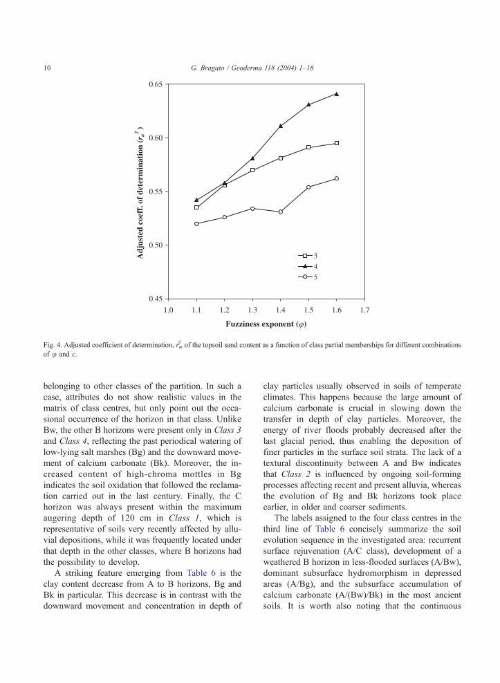
Fig. 4. Adjusted coefficient of determination, ra2, of the topsoil sand content as a function of class partial memberships for different combinations

of u and c.


belonging to other classes of the partition. In such a

case, attributes do not show realistic values in the

matrix of class centres, but only point out the occa-

sional occurrence of the horizon in that class. Unlike

Bw, the other B horizons were present only in Class 3

and Class 4, reflecting the past periodical watering of

low-lying salt marshes (Bg) and the downward move-

ment of calcium carbonate (Bk). Moreover, the in-

creased content of high-chroma mottles in Bg

indicates the soil oxidation that followed the reclama-

tion carried out in the last century. Finally, the C

horizon was always present within the maximum

augering depth of 120 cm in Class 1, which is

representative of soils very recently affected by allu-

vial depositions, while it was frequently located under

that depth in the other classes, where B horizons had

the possibility to develop.

A striking feature emerging from Table 6 is the

clay content decrease from A to B horizons, Bg and

Bk in particular. This decrease is in contrast with the

downward movement and concentration in depth of

clay particles usually observed in soils of temperate

climates. This happens because the large amount of

calcium carbonate is crucial in slowing down the

transfer in depth of clay particles. Moreover, the

energy of river floods probably decreased after the

last glacial period, thus enabling the deposition of

finer particles in the surface soil strata. The lack of a

textural discontinuity between A and Bw indicates

that Class 2 is influenced by ongoing soil-forming

processes affecting recent and present alluvia, whereas

the evolution of Bg and Bk horizons took place

earlier, in older and coarser sediments.

The labels assigned to the four class centres in the

third line of Table 6 concisely summarize the soil

evolution sequence in the investigated area: recurrent

surface rejuvenation (A/C class), development of a

weathered B horizon in less-flooded surfaces (A/Bw),

dominant subsurface hydromorphism in depressed

areas (A/Bg), and the subsurface accumulation of

calcium carbonate (A/(Bw)/Bk) in the most ancient

soils. It is worth also noting that the continuous

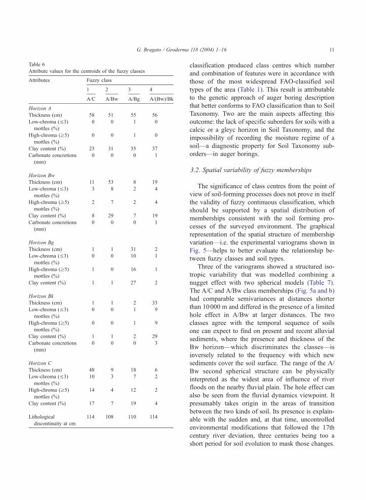
Table 6

Attribute values for the centroids of the fuzzy classes

Attributes Fuzzy class

1 2 3 4

A/C A/Bw A/Bg A/(Bw)/Bk

Horizon A

Thickness (cm) 58 51 55 56

Low-chroma (V3)

mottles (%)

0 0 1 0

High-chroma (z5)

mottles (%)

0 0 1 0

Clay content (%) 23 31 35 37

Carbonate concretions

(mm)

0 0 0 1

Horizon Bw


Low-chroma (V3)

mottles (%)

3 8 2 4

High-chroma (z5)

mottles (%)

2 7 2 4

Clay content (%) 8 29 7 19


(mm)

0 0 0 1

Horizon Bg


Low-chroma (V3)

mottles (%)

0 0 10 1

High-chroma (z5)

mottles (%)

1 0 16 1


Horizon Bk


Low-chroma (V3)

mottles (%)

0 0 1 9

High-chroma (z5)

mottles (%)

0 0 1 9



(mm)

0 0 0 3

Horizon C


Low-chroma (V3)

mottles (%)

10 3 7 2

High-chroma (z5)

mottles (%)

14 4 12 2


Lithological

discontinuity at cm

114 108 110 114


classification produced class centres which number

and combination of features were in accordance with

those of the most widespread FAO-classified soil

types of the area (Table 1). This result is attributable

to the genetic approach of auger boring description

that better conforms to FAO classification than to Soil

Taxonomy. Two are the main aspects affecting this

outcome: the lack of specific suborders for soils with a

calcic or a gleyc horizon in Soil Taxonomy, and the

impossibility of recording the moisture regime of a

soil—a diagnostic property for Soil Taxonomy sub-

orders—in auger borings.

3.2. Spatial variability of fuzzy memberships

The significance of class centres from the point of

view of soil-forming processes does not prove in itself

the validity of fuzzy continuous classification, which

should be supported by a spatial distribution of

memberships consistent with the soil forming pro-

cesses of the surveyed environment. The graphical

representation of the spatial structure of membership

variation—i.e. the experimental variograms shown in

Fig. 5—helps to better evaluate the relationship be-

tween fuzzy classes and soil types.

Three of the variograms showed a structured iso-

tropic variability that was modelled combining a

nugget effect with two spherical models (Table 7).

The A/C and A/Bw class memberships (Fig. 5a and b)

had comparable semivariances at distances shorter

than 10000 m and differed in the presence of a limited

hole effect in A/Bw at larger distances. The two

classes agree with the temporal sequence of soils

one can expect to find on present and recent alluvial

sediments, where the presence and thickness of the

Bw horizon—which discriminates the classes—is

inversely related to the frequency with which new

sediments cover the soil surface. The range of the A/

Bw second spherical structure can be physically

interpreted as the widest area of influence of river

floods on the nearby fluvial plain. The hole effect can

also be seen from the fluvial dynamics viewpoint. It

presumably takes origin in the areas of transition

between the two kinds of soil. Its presence is explain-

able with the sudden and, at that time, uncontrolled

environmental modifications that followed the 17th

century river deviation, three centuries being too a

short period for soil evolution to mask those changes.

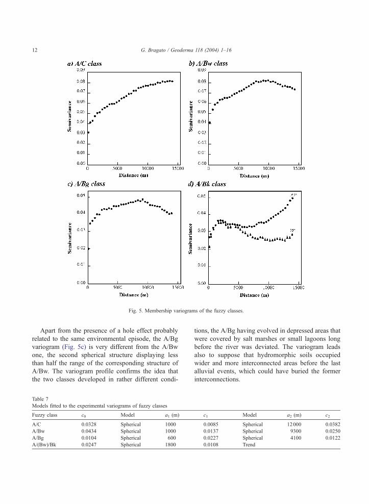
Fig. 5. Membership variograms of the fuzzy classes.


Apart from the presence of a hole effect probably

related to the same environmental episode, the A/Bg

variogram (Fig. 5c) is very different from the A/Bw

one, the second spherical structure displaying less

than half the range of the corresponding structure of

A/Bw. The variogram profile confirms the idea that

the two classes developed in rather different condi-

Table 7

Models fitted to the experimental variograms of fuzzy classes

Fuzzy class c0 Model a1 (m)

A/C 0.0328 Spherical 1000

A/Bw 0.0434 Spherical 1000

A/Bg 0.0104 Spherical 600

A/(Bw)/Bk 0.0247 Spherical 1800

tions, the A/Bg having evolved in depressed areas that

were covered by salt marshes or small lagoons long

before the river was deviated. The variogram leads

also to suppose that hydromorphic soils occupied

wider and more interconnected areas before the last

alluvial events, which could have buried the former

interconnections.

c1 Model a2 (m) c2

0.0085 Spherical 12000 0.0382

0.0137 Spherical 9300 0.0250

0.0227 Spherical 4100 0.0122

0.0108 Trend

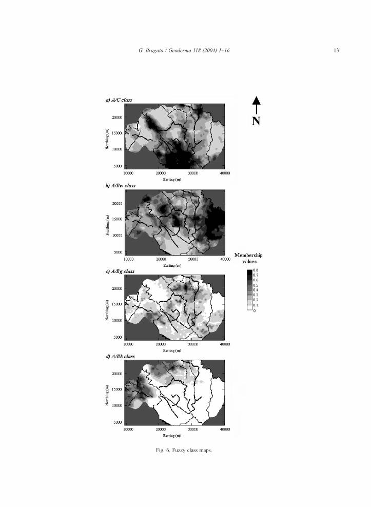
Fig. 6. Fuzzy class maps.



Unlike the former classes, the A/(Bw)/Bk vario-

gram (Fig. 5d) shows a composite spatial variability,

characterized by a marked anisotropic trend at 165j,roughly corresponding to the WNW–ESE river direc-

tion. The peculiar shape of the variogram appears to be

related to the outlying location of soil individuals with

a Bk horizon—clustered in the north-western portion

of the surveyed area—and the spatial continuity with

upstream soil types, where the A/(Bw)/Bk sequence is

predominant (Ente di Sviluppo Agricolo del Veneto,

1996b) and the River Piave forms a sort of boundary

between homologous areas.

3.3. Fuzzy class and composite maps

The continuous class maps of Fig. 6 clarify the

meaning of variograms in terms of membership

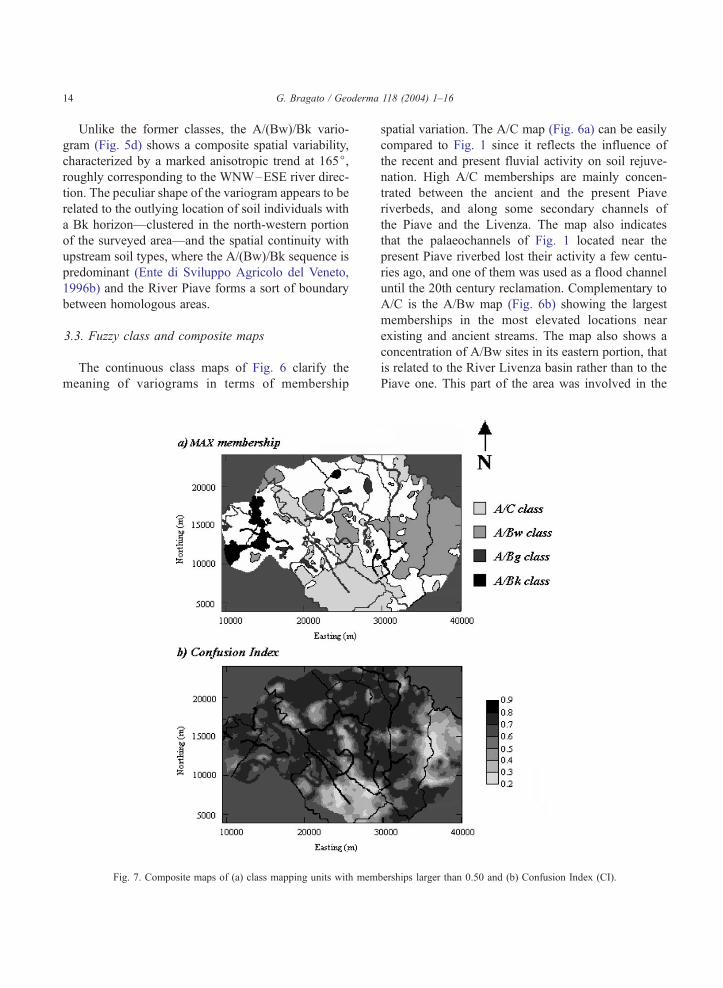
Fig. 7. Composite maps of (a) class mapping units with mem

spatial variation. The A/C map (Fig. 6a) can be easily

compared to Fig. 1 since it reflects the influence of

the recent and present fluvial activity on soil rejuve-

nation. High A/C memberships are mainly concen-

trated between the ancient and the present Piave

riverbeds, and along some secondary channels of

the Piave and the Livenza. The map also indicates

that the palaeochannels of Fig. 1 located near the

present Piave riverbed lost their activity a few centu-

ries ago, and one of them was used as a flood channel

until the 20th century reclamation. Complementary to

A/C is the A/Bw map (Fig. 6b) showing the largest

memberships in the most elevated locations near

existing and ancient streams. The map also shows a

concentration of A/Bw sites in its eastern portion, that

is related to the River Livenza basin rather than to the

Piave one. This part of the area was involved in the

berships larger than 0.50 and (b) Confusion Index (CI).


post-glacial, west-to-east translation of the Livenza,

after which the Bw horizon had enough time to

develop. The A/Bg memberships (Fig. 6c) show a

patchy spatial distribution. Larger values are generally

located in depressed, formerly flooded areas that

characterized most of the north-western Adriatic coast

in the past. The map suggests that only part of these

areas had been permanently flooded, the remaining

portions being only seasonally inundated. As already

indicated by the variogram, a peculiar distribution is

displayed by the A/(Bw)/Bk class (Fig. 6d). Even if

the inadequate variogram modellization of the A/

(Bw)/Bk class affects interpolation, the concentration

of A/(Bw)/Bk elements reflects the splitting of the

most ancient soils of the area in two subareas due to

the recent and present fluvial activity.

The composite maps obtained with the MAX

operator and the Confusion Index are shown in

Fig. 7. The MAX membership map (Fig. 7a) was

drawn after selecting a partial membership threshold

of 0.50 as the lower membership value for homoge-

neous mapping units. This map summarizes the

continuous class maps of Fig. 6, delineating the

mapping units that are influenced by the prevalent

effect of a single soil-forming process from those

affected by different, simultaneous or sequential

processes, the classification of which should be

carefully evaluated. The most recent processes,

pointed out by the A/C and the A/Bw classes,

prevail all over the area, whereas marked signs of

long-lasting phenomena are relegated to the northern

part of the map.

Areas with high soil heterogeneity can be delin-

eated with the CI map of Fig. 7b. High CI values

indicate locations where continuous classes overlap,

providing information complementary to the MAX

membership map. Class allocation is confusing along

the watershed between Piave and Livenza Rivers in

the eastern part of the map, where floods from both

rivers alternatively covered the soil surface. High CI

values are also present in the north-western border of

the lagoon and along the palaeochannels of Fig. 1,

characterizing locations affected by recent sedimen-

tary events that covered already developed soils. The

joint use of the two composite maps may translate

the results of FCM into the syntax of discrete,

already existing classifications. In this study, the

MAX membership map helps to delineate mapping

units that in the first instance correspond to FAO soil

types originated by a single soil-forming process.

The CI map may embody additional information on

the spatial distribution of class intergrades that the

existing classification catalogue as soil intergrades.

Riverbed translation due to tectonic subsidence, for

example, is a factor involved in FAO Fluvic Cambi-

sols genesis. It is also the process responsible for the

presence of the A/C to A/Bw class intergrades in the

investigated area, and the CI map of Fig. 7b could

be used for a first delineation of this Fluvisols to

Cambisols intergrade in the lower Piave fluvial

plain.

4. Conclusions

The combination of fuzzy c-means clustering and

geostatistical techniques improves the interpretation

of field data when the transition of a soil from one

type to another is gradual and not easily observable

on the surface. The obtained results are explainable

in terms of local soil-forming processes and can be

used for a first soil map delineation. The proposed

approach does not rule out remote sensing and

aerial photogrammetry. It might represent, on the

contrary, part of a complex analytical sequence

capable of using both sources of information—the

pattern soil fuzzy classes and the landform analy-

sis—to formulate a spatially detailed territorial mod-

el that should represent the basic level of informa-

tion for a locally oriented land use assessment. A

further investigative step of the present case study

will be its comparison with the results of the

detailed geomorphological analysis, in due course

at present.

Acknowledgements

I wish to thank Veneto Agricoltura and the

Provincia di Venezia, Dr. A. Vitturi and Dr. B. Basso

in particular, which kindly provided the soil data set

used in the present study. I am grateful to Dr. J.J. de

Gruijter, Alterra, for his helpful suggestions and his

comments on the draft version of the manuscript. I am

also grateful to Dr. D.J.J. Walvoort, Alterra, for the

compositional kriging program. This work was


supported by a research fellowship of the Organisa-

tion for Economic Cooperation and Development

(OECD).

References

Baize, D., Girard, M.C., 1995. Referentiel Pedologique. INRA Edi-

tions, Versailles, p. 332.

Bezdek, J.C., 1981. Pattern Recognition with Fuzzy Objective

Function Algorithms. Plenum, New York.

Boldesan, A., 2000. I fiumi, le lagune e il mare: la geomorfologia

della Pianura. In: Bondesan, A., Caniato, G., Vallerani, F.,

Zanetti, M. (Eds.), Il Piave, Cierre Edizioni, Sommacampagna

(VR), pp. 76–86.

Burrough, P.A., van Gaans, P.F.M., Hoostmans, R., 1997. Contin-

uous classification in soil survey: spatial correlation, confusion

and boundaries. Geoderma 77, 115–135.

Carre, F., Girard, M.C., 2002. Quantitative mapping of soil types

based on regression kriging of taxonomic distances with land-

form and land cover attributes. Geoderma 110, 241–263.

Costantini, E.A.C., Campostrini, F., Arcara, P.G., Cherubini, P.,

Storchi, P., Pierucci, M., 1996. Soil and climate functional char-

acters for grape ripening and wine quality of ‘‘Vino Nobile di

Montepulciano’’. Acta Hort. 427, 45–55.

de Bruin, S., Stein, A., 1998. Soil-landscape modelling using fuzzy

c-means clustering of attribute data derived from a Digital Ele-

vation Model (DEM). Geoderma 83, 17–33.

de Gruijter, J.J., Walvoort, D.J.J., van Gaans, P.F.M., 1997. Contin-

uous soil maps—a fuzzy set approach to bridge the gap between

aggregation levels of process and distribution models. Geoderma

77, 169–195.

Ente di Sviluppo Agricolo del Veneto, 1996a. I suoli dell’area a

DOC del Piave. Provincia di Venezia. Centro Servizi Editoriali

ESAV, Padova.

Ente di Sviluppo Agricolo del Veneto, 1996b. I suoli dell’area a

DOC del Piave. Provincia di Treviso. Centro Servizi Editoriali

ESAV, Padova.

FAO-UNESCO, 1994. Soil Map of the World. Revised Legend.

FAO, Roma.

Geovariances, 2000. ISATIS Software Manual. Eds. Geovariances,

Avon, France. 591 pp.

Hudson, B.D., 1992. The soil survey as paradigm-based science.

Soil Sci. Soc. Am. J. 56, 836–841.

Istituto Sperimentale per lo Studio e la Difesa del Suolo, 1995.

Manuale per il rilevamento del suolo ISSDS, Firenze.

Jenny, H., 1941. Factors of Soil Formation. McGraw-Hill, New

York.

Lagacherie, P., Andrieux, P., Bouzigues, R., 1996. Fuzziness and

uncertainty of soil boundaries: from reality to coding in GIS.

In: Bourrough, P.A., Frank, A.U. (Eds.), Geographic Objects

with Indeterminate Boundaries. Taylor & Francis, London,

pp. 275–286.

Lagacherie, P., Cazemier, D.R., van Gaans, P.F.M., Burrough, P.A.,

1997. Fuzzy k-means clustering of fields in an elementary catch-

ment and extrapolation to a larger area. Geoderma 77, 197–216.

Lebon, E., Dumas, V., Morlat, R., 1997. Influence des facteurs

natureles du terroir sur la maturation du raisin en Alsace. 1er

Colloque Internationale ‘‘Les terroirs viticoles’’. INRA, Angers,

pp. 359–366.

Mazaheri, S.A., Koppi, A.J., McBratney, A.B., 1995. A fuzzy allo-

cation scheme for the Australian great soil groups classification

system. Geoderma 46, 601–612.

McBratney, A.B., de Gruijter, J.J., 1992. A continuum approach to

soil classification and mapping: classification by modified fuzzy

k-means with extragrades. J. Soil Sci. 43, 159–175.

McBratney, A.B., Moore, A.W., 1985. Application of fuzzy sets to

climatic classification. Agric. For. Meteorol. 35, 165–185.

McBratney, A.B., de Gruijter, J.J., Brus, D.J., 1992. Spatial predic-

tion and mapping of continuous soil classes. Geoderma 54,

39–64.

Milligan, G.W., 1996. Clustering validation: results and implica-

tions for applied analyses. In: Arabic, P., Hubert, L.J., de Soete,

G. (Eds.), Clustering and Classification. World Scientific Publ.,

River Edge, NJ, pp. 341–375.

Minasny, B., McBratney, A.B., 1999. FuzME version 1.0, Fuzzy k-

means with extragrades program. Australian Centre for Preci-

sion Agriculture. The University of Sidney, Australia. http://

www.usyd.edu.au/su/agric/acpa/pag.htm.

Ministero per le Politiche Agricole e Forestali, 2000. Metodi di

analisi chimica del suolo. Franco Angeli, Milano.

Odeh, I.O.A., McBratney, A.B., Chittleborough, D.J., 1992. Soil

pattern recognition with fuzzy c-means: application to classifi-

cation and soil landform interrelationships. Soil Sci. Soc. Am. J.

56, 505–516.

Pawlowsky, V., Olea, R.A., Davis, J.C., 1995. Estimation of region-

alized compositions: a comparison of three methods. Math.

Geol. 27, 105–127.

Rossiter, D.G., 1996. A theoretical framework for land evaluation.

Geoderma 72, 165–202.

Sangalli, A., 1998. The Importance of Being Fuzzy and Other In-

sights from the border between math and computers. Princeton

Univ. Press, Princeton, NJ.

Soil Survey Staff, 1994. Keys to Soil Taxonomy, 6th ed. USDA-

Soil Conservation Service. U.S. Govt. Print. Office, Washing-

ton, DC.

Triantafilis, J., Ward, W.T., Odeh, I.O., McBratney, A.B., 2001.

Creation and interpolation of continuous soil layer classes in

the Lower Namoi Valley. Soil Sci. Soc. Am. J. 65, 403–413.

Verheyen, K., Dries, A., Hermy, M., Deckers, S., 2001. High-res-

olution continuous soil classification using morphological soil

profile descriptions. Geoderma 101, 1–48.

Walvoort, D.J.J., de Gruijter, J.J., 2001. Compositional kriging: a

spatial interpolation method for compositional data. Math. Geol.

33, 951–966.

Zimmerman, H.J., 1996. Fuzzy Sets Theory and Its Applications,

3rd ed. Kluwer Academic Publishing, Boston.

http:\\www.usyd.edu.au\su\agric\acpa\pag.htm

fuzzy continuous classification and spatial interpolation in conventional soil survey for soil...

Documents