futures trading and investor returns: an investigation of commodity market risk premiums

Futures Trading and Investor Returns: An Investigation of Commodity Market RiskPremiumsAuthor(s): Katherine DusakSource: Journal of Political Economy, Vol. 81, No. 6 (Nov. - Dec., 1973), pp. 1387-1406Published by: The University of Chicago PressStable URL: http://www.jstor.org/stable/1830746 .

Accessed: 29/04/2014 15:00

Your use of the JSTOR archive indicates your acceptance of the Terms & Conditions of Use, available at .http://www.jstor.org/page/info/about/policies/terms.jsp

.JSTOR is a not-for-profit service that helps scholars, researchers, and students discover, use, and build upon a wide range ofcontent in a trusted digital archive. We use information technology and tools to increase productivity and facilitate new formsof scholarship. For more information about JSTOR, please contact [email protected].

.

The University of Chicago Press is collaborating with JSTOR to digitize, preserve and extend access to Journalof Political Economy.

http://www.jstor.org

This content downloaded from 109.241.198.166 on Tue, 29 Apr 2014 15:00:43 PMAll use subject to JSTOR Terms and Conditions

http://www.jstor.org/action/showPublisher?publisherCode=ucpress

http://www.jstor.org/stable/1830746?origin=JSTOR-pdf

http://www.jstor.org/page/info/about/policies/terms.jsp


Futures Trading and Investor Returns: An Investigation of Commodity Market Risk Premiums

Katherine Dusak Chicago, Illinois

The long-standing controversy over whether speculators in a futures market earn a risk premium is analyzed within the context of the capital asset pricing model recently developed by Sharpe, Lintner, and others. Under that approach the risk premium required on a futures contract should depend not on the variability of prices but on the extent to which the variations in prices are systematically related to variations in the return on total wealth. The systematic risk was estimated for a sample of wheat, corn, and soybean futures contracts over the period 1952 to 1967 and found to be close to zero in all three cases. Average realized holding period returns on the contracts over the same period were close to zero.

I. Introduction

Considerable controversy exists over the amount and the nature of the returns earned by speculators in commodity futures markets. At one extreme is the position first set forth by J. M. Keynes in his Treatise on Money (1930, pp. 135-44) that a futures market is an insurance scheme in which the speculators underwrite the risks of price fluctuation of the spot commodity. The nonspeculators or "hedgers" on the other side of the market must expect to pay and, according to Keynes, they do in fact pay, on the average a significant premium to the speculator-insurers for this service. At the other extreme have been those such as C. 0. Hardy (1940) who argue that for many speculators a futures market is a gambling casino. Far from demanding and receiving compensation for

I am indebted to Eugene Fama, Charles Nelson, Harry Roberts, and especially Merton H. Miller for many helpful comments and suggestions.

1387



1388 JOURNAL OF POLITICAL ECONOMY

taking over the risks of price fluctuation from the hedgers, speculators, as a class, are willing to pay for the privilege of gambling in this socially acceptable form (with the losers continually being replaced at the tables by new arrivals). Despite many empirical studies, the conflict between the insurance interpretation and the gambling interpretation of returns to speculators in futures markets remains unresolved.'

This paper offers another and quite different interpretation of the returns to speculators in futures markets. It is argued that futures markets are no different in principle from the markets for any other risky portfolio assets. Futures markets are perhaps more colorful than many other sub- segments of the capital market such as the New York Stock Exchange or the bond market, and the terminology of futures markets is perhaps more arcane, but these differences in form should not obscure the fundamental properties that futures market assets share with other investment instruments: in particular, they are all candidates for inclusion in the investor's portfolio.

The portfolio approach, by itself, makes no presumption as to whether returns to speculators are positive, as Keynes hypothesized, or zeroish to negative, as Hardy believed. It says, rather, that returns on any risky capital asset, including futures market assets, are governed by that asset's contribution, positive, negative, or zero, to the risk of a large and well- diversified portfolio of assets (in fact, all assets, in principle). In contrast to this portfolio measure of risk, Keynes and his later followers identify the risk of a futures market asset solely with its price variability.2 These differences in the proposed measures of risk make it possible to test the portfolio and Keynesian interpretations of futures markets against each other and, in principle, also against the Hardy gambling casino view.

It turns out that for each of the commodity futures studied (wheat, corn, and soybeans) returns and portfolio risk are both close to zero during the sample period even though variability or risk in the Keynesian sense is high. Hence, as far as this set of observations is concerned, the data conform better to the portfolio point of view than to the Keynesian insurance interpretation. The sample did not permit any direct confrontation between the portfolio interpretation and the Hardy view, but some indirect light is thrown on this part of the controversy and some suggestions for further tests are offered.

I Among the most influential papers devoted to the Keynes-Hardy controversy have been those of Telser (1958, 1960, 1967) and Cootner (1960a, 1960b). Other studies of the returns to speculation in futures markets include Houthakker (1957), Gray (1961), Smidt (1965), Rockwell (1967), and Stevenson and Bear (1970).

2 This is at least the conventional interpretation of the Keynesian position as suggested by the following quotation: "It will be seen that, under the present regime of very widely fluctuating prices for individual commodities, the cost of insurance against price changes -which is additional to any charges for interest or warehousing-is very high" (Keynes 1930, p. 144). A somewhat broader interpretation emphasizes the insurance premium and tries to relate the size and sign of this premium to variations in the stocks of the commodity over the production cycle (see Cootner 1960a, 196Gb).



TRADING AND INVESTOR RETURNS I 389

In the next section the salient points of the equilibrium pricing of portfolio assets are noted, and futures contracts are analyzed within this context. Measures of Keynesian and portfolio asset risk are then developed and interpreted in the light of the returns observed.

II. Capital Asset Pricing: The Determination of an Equilibrium Risk-Return Relation

A model of the equilibrium pricing of portfolio assets was proposed originally by Sharpe (1964) and extended by Lintner (1965), Mossin (1966), and Fama (1971). Sharpe showed that conditions exist under which the equilibrium risk-return relation for any capital asset i can be represented as

E( = Rf E+ ( Rw) Rj a (R "), (1)

where Ri is the random rate of return on asset i, E(Ri) is its math- ematical expectation, and Rf is the pure time return to capital or the so- called riskless rate of interest; RW is the random rate of return on a representative dollar of total wealth or, equivalently, the return on a portfolio containing all existing assets in the proportions, xi, in which they are actually outstanding: E (RW) is the expected rate of return on total wealth, and (Kw), the standard deviation of the return on total wealth, is a measure of the risk involved in holding a representative dollar of total wealth. The term [0u(K,)1/axi is the marginal contribution of asset i to the risk of the return on total wealth) U(Rw). Thus expression (1) says that, in equilibrium, the expected rate of return on any asset i will be equal to the riskless rate of interest plus a risk premium proportional to the contribution of the asset to the risk of the return on total wealth.

To see some of the broader implications of this proposition and especially to highlight its fundamental difference from the simple Keynesian approach to risk, note that since

-N

(Rw) =L E xixj CoV (Pi, Rj) _i-l j=l

it follows that

____ ̂ _ ____ Fv' xi Cov (Rin R .)l

ox aW) L1t j C

3 The description of the equilibrium pricing model presented here assumes some familiarity on the part of the reader. For a more complete discussion, see Sharpe (1964) or Lintner (1965). A detailed exposition of the model is also given in Famna and Miller (1972, chap. 7).I



I 390 JOURNAL OF POLITICAL ECONOMY

Thus what governs the riskiness of any asset i is not merely its own variance c2(ki) but its weighted covariance with all the other assets making up total wealth. Normally the latter terms can be expected to swamp the former, since there are N - 1 terms making up the covariance portion and only one in the variance portion, and that one, moreover, weighted by a very small number, xi.

Additional insight into the equilibrium risk-return relation is gained by noting that the expression

N

E xi CoY (Ri, Rj) j=1

can be rewritten as Cov (Ri, kw), the covariance of return on asset i with that of total wealth. Hence we can rewrite (1) as

E(R ) -R +E(f - Rf Cov (Ri, R,,) (2) L W~R) J u(R?) or equivalently as

E(Ri) - Rf - [E(R~w) -Rf]flj (3)

where fi5= [CoV (i), kw)]/Io2(kw). The coefficient fi can be interpreted as the relative risk of asset i, since it measures the risk of asset i relative to that of total wealth. Equation (3) then says that the risk premium expected on asset i is proportional, in equilibrium, to its systematic risk fli, the factor of proportionality being the risk premium expected on a representative dollar of total wealth.

Needless to say, the capital asset pricing model rests on a set of fairly strong assumptions. Nevertheless, it has proven to be remarkably robust empirically. Studies by Miller and Scholes (1972), Black, Jensen, and Scholes (1972), and Fama and MacBeth (1972) indicate that while simple expressions such as equations (2) and (3) may not be entirely satisfactory descriptions of the relations between return and relative risk, there is a strong connection between them, whereas there seems to be virtually none between the risk premium and measures of nonportfolio

*. 4 risk.4

III. Application of the Capital Asset Pricing Model to Futures Contracts

One difficulty in applying the Sharpe model of capital asset pricing to the risk-return relation on futures contracts is that of defining the ap-

' Recently Black (1972) has generalized the Sharpe model by replacing the riskless asset having return Rf with another asset whose return is a random variable but whose covariance with total wealth is zero. Empirical tests by Black, Jensen, and Scholes (1972) and Fama and Macbeth (1972) seem to indicate that the generalized model fits the data somewhat better than the Sharpe version.



TRADING AND INVESTOR RETURNS 1391

propriate capital asset and its rate of return. Since virtually all futures contracts are bought (and sold short) on margins that typically range from 5 to 10 percent of the face value of the contract, it might seem at first sight that we can treat the margin as the capital investment and treat the ratio of the net profit at closeout to the initial margin as the rate of return on investment. In fact, one theoretical study, that of Schrock (1971), takes this point of view and makes it the basis of a standard mean-variance portfolio analysis, a la Markowitz (1959), though restricting attention only to futures market assets.

This appealing procedure for computing futures market returns breaks down, however, as soon as we trace the subsequent history of the payment that is turned over to the broker. Unlike other capital assets such as common stocks where the margin is transferred from buyer to seller, the margin on a futures contract is kept in escrow by the broker. Not only does the seller of the futures contract not receive the capital transfer from the buyers, but he actually has to deposit an equivalent amount of his own funds in the broker's escrow account. At closeout, the broker returns the escrowed margin plus or minus any profits or losses (net of commissions in the case of profits and inclusive of commissions in the event of losses) that occurred over the period.

The margin, despite surface appearances, is thus not a portfolio asset in the sense of the Sharpe general-equilibrium model, but merely a good- faith deposit to guarantee performance by the parties to the contract. If the brokers had other ways of ensuring that traders did not make commit- ments beyond their resources, then no such performance bonds would be required. For example, forward foreign exchange markets, where firms deal through their own banking connections, typically operate without any explicit margins, whereas participants in public futures currency markets are required to post margins. 5

Although the rate of return on the margin is not a ineaningful number from a general-equilibrium point of view, and need not even exist if other

That entering into a future contract need involve no margin or other specific payment that could be interpreted as an "investment" (and hence that could serve as the basis for computing a "rate of return") does not mean that the mean-svariance portfolio model cannot be applied at the microlevel to analyze an investor's decision process. The price changes on the contracts held will affect terminal wealth, just as in the case of any other asset; but the contracts do not appear in the initial wealth constraint. For a rigorous treatment in the context of forward foreign exchange, see Leland (1971). A study by Johnson (1960) of futures spot commodity holdings also proceeds in this way. That is, the entire analysis is conducted in terms of price changes and not in terms of rates of return. The fact that the margin does not really represent capital invested in futures contracts, even in those markets where margin is required, might perhaps have been appreciated earlier by analysis of futures markets trading if brokers paid interest on the escrowed funds (or, what amounts to the same thing, if they allowed all traders to deposit or to hypothecate income-earning assets rather than cash). In practice, of course, the brokers presumably do pay interest on the escrowed funds, but only in the hard-to-see form of lower commissions or higher levels of "free" services than would otherwise be the case.




types of guarantees could serve, there is another natural candidate which can always be computed: namely, the percentage change in the futures price. We cannot interpret this percentage change as a rate of return comparable to the Ra, in .equation (2) above, since the holder invests no current resources in the contract. But we can interpret it as essentially the risk premium, hi - Rf, on the spot commodity.6

What corresponds to the full return Ri is the return (net of storage costs) that would accrue to the holder of an unhedged spot commodity.7 That return consists of interest on the capital invested in the commodity plus any return, positive or negative, over and above pure interest due to the unanticipated change in the price of the commodity. If the spot holder chooses to hedge his holding, he thereby converts it to a riskless asset on which he earns only the riskless rate, Rf. The purchaser of the futures contract who takes over the risk has no capital of his own invested and hence earns no interest or pure time return on capital. He receives only the return over and above interest, which is to say, Ri- Rf.

This argument can be formalized by restating the Sharpe equilibrium conditions in present-value form. We say that the expected return on any asset i can be expressed as

E(Ki) = (1 - fi)Rf + fliE(i2w), (4) where fpi = Cov (Ri, Rw)/af2(fR). Equivalently, since we can represent E (hi) in terms of period 0 and period 1 prices for the asset as [E(Pi,) -

PijoJ lPis0, the equilibrium risk-return relation on asset i can be expressed as = E(Pisl) - [E(/?w) - Rf]Pi o/3 (5)

(1 + Rf) Expression (5) says that the current price of any asset i is the discounted value (at the riskless rate) of its expected period 1 price, adjusted down- ward for risk by the factor [E(i,,) - Rf]Pi ,),.

Now suppose one were interested in knowing the price of asset i under a contractual agreement to purchase the asset at time 0 but with payment deferred a period to time 1. Clearly the current price for the asset under such an agreement must be given by Pi0(1 + Rf). That is, since the

6 I abstract from such complications as transaction costs, basis risk, the business risk of the storage and processing industries, limitations on borrowing, and so on. Or, what amounts to the same thing, I assume that differences in the returns on spot and futures market assets from these sources are so small and so unsystematic relative to the variations in returns on both assets as a consequence of price fluctuations that they can safely be ignored in a first approximation. Some of the main second-order qualifications are indicated at various points in the text and in footnotes in the course of the discussion.

7 Actually total return to the spot commodity holder can be decomposed into three components: a pure time return to capital, a risk premium, and remuneration for storage costs, defined in this context as insurance charges, spoilage, and warehousing and administrative costs. Since we are concerned only with the return to capital embodied in the spot commodity, Ri, the "full" return on the spot commodity is to be understood as net of storage costs.




transaction is made at time 0 but consummated at time 1, the purchaser must pay a one-period credit, or borrowing charge of P IoRf in addition to the current price Pi,0. Multiplying both sides of equation (5) by (1 + Rf)we seethat

Pio(l + Rf) = E(Pi~l) - [E(Rw) - Rf]Pifof3. (6) But the contractual agreement just described is a futures contract

where asset i refers to the spot commodity. Hence the expression Pio(l + Rf) can be interpreted as the current futures price for delivery and payment of the spot commodity one period later, and E(P 1) can be interpreted as the spot price expected to prevail at time 1. The essen- tial point is that buying a futures contract is like buying a capital asset on credit where the capital asset in this case happens to be the spot commodity.8 The only issue is what is the "discount for cash" or, equivalently, the financing charge. Since the financing is assumed to be riskless, the correct charge is clearly Rf. That is, if P1 0 is the current price for immediate payment, Piof(l + RIf) must be the price if the buyer buys on one-period credit terms.

Setting Pf0 = Pi1o(l + Rf) and rearranging terms, we get

E(P.,) - Pfo = flAeE(I j2) - Rf]. (7) PiO

Equation (7) can be interpreted as expressing the risk premium on the spot commodity as the change in the futures price divided by the period 0 spot price. Thus once again we see that futures contracts, properly interpreted, pose no problem for capital market theory.

One implication of this analysis is that there are two essentially equivalent ways of calculating the risk premium. On the one hand, we can try to measure the risk premium by taking the percentage change in spot prices (net of storage) over a given interval minus the riskless rate. Alternatively, we can approximate the risk premium as the percentage change in the futures price over the same interval.9 Of these two approaches, it is the latter that will be adopted here. Data on futures prices

8 It does not really matter whether there is a spot commodity in existence yet. That is, just as I can order a car not yet produced. so I can agree to accept delivery next period at a specified price of a commodity still unproduced. The "implicit" spot price, which always exists, is then simply the futures price minus a discount for payment in advance, i.e., Pi = Pf/(l + Rf). Note also that the seller need not actually contemplate produc- ing the spot commodity; i.e., he can be a pure short speculator. He merely offers to make delivery to you next period, intending, if necessary to go out and buy the spot commodity then, if you insist on delivery rather than settlement.

9 I have argued that in equilibrium Pf,, = Pi,,(l + Rf), where i refers to the spot commodity. Thus the percentage change in the futures price underestimates the risk premium on the spot commodity by the factor 1/(1 + Rf). Given the intervals over which I will be computing returns, the factor 1/(1 + Rr) is likely to be very small. Hence for simplicity of exposition I shall refer (somewhat loosely) to the percentage change in the futures price as representing the risk premium on the spot commodity.




are more accessible than spot price data and, of course, use of futures prices also avoids the necessity of having to estimate the storage costs directly. It is important to remember, however, that this choice of measurement is essentially a matter of computational convenience; and that the relevant risk from the general-equilibrium point of view remains the risk inherent in the ownership of the spot commodity itself, regardless of who actually chooses to bear it or what measurement strategy we choose to employ. 10

IV. The Empirical Properties of Futures Market Returns

Tests of the risk-return relationship in the futures market are based on a sample of three heavily traded agricultural commodities: wheat, corn, and soybeans. There are five different contracts per year for wheat and corn and six for soybeans. For all contracts, semimonthly price quotations were obtained for a 15-year period from May 15, 1952 through Novem- ber 15, 1967--resulting in an approximate sample size of 300 observations per contract. " In all cases returns were computed as a simple 2-week holding period yield with no allowance made for transaction costs. Following universal practice, returns have been computed separately for each commodity contract (e.g., May wheat or September corn).1 2 It should be noted that the return series computed in this way is dis- continuous, since published price quotations on any one contract are typically available over a 9- or 1 0-month span.

10 I have assumed that unanticipated changes in the spot and futures prices are perfectly correlated. (For some evidence on the high degree of correlation between spot and futures prices, see Houthakker [1968].) Where this correlation is not perfect, the spot commodity holder will bear some risk even though hedged, and some compensation for this risk may be impounded in his return. Working (1953) has made this type of risk central to his analysis of futures markets. He regards spot commodity holders not as passive short hedgers but as speculators on the movement of the spot-future price dif- ferential, or basis, over timee. He argues that professional commodity dealers are better able to predict differentials or relative prices than price levels. Thus they assume a position in both the spot and futures markets in response to expected changes in the basis. Since Working's hypothesis appears to have no testable implications with respect to the risk- return relation in futures markets of the kind that are of main concern in this paper, I will not pursue it further here.

I" Price quotations were taken from U.S., Department of Agriculture (1952-67). Lester Telser kindly supplied price data for 1952-64. The rest were collected indepen- dently from the same source. The terminal date of 1967 was the last year for which price data were available at the time this study was started. The initial date of 1952 was chosen to minimize wartime and postwar controls on commodity prices and futures trading.

12 Another possible principle for computing returns would be on the basis of time to contract expiration (e.g., wheat contracts with exactly 4 months to run or corn contracts with 22 months to run). In a later paper I shall show that the theoretical and empirical justification for looking at returns in this way is weaker than certain treatments of the matter, notably Samuelson's (1965), would suggest.



TRADING AND INVESTOR RETURNS I395

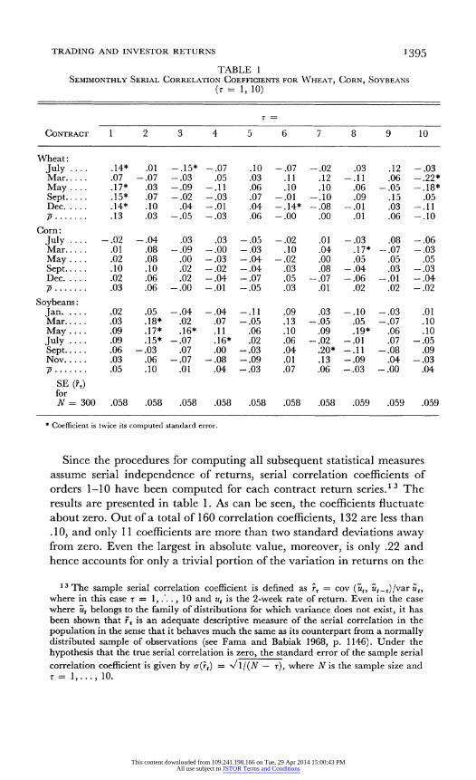
TABLE 1 SEMIMONTHLY SERIAL CORRELATION COEFFICIENTS FOR WHEAT, CORN, SOYBEANS

(r = 1, 10)

CONTRACT 1 2 3 4 5 6 7 8 9 10

Wheat: July .... .14* .01 -.15* -.07 .10 -.07 -.02 .03 .12 -.03 Mar.... . .07 -.07 -.03 .05 .03 .11 .12 -.11 .06 -.22* May .... .17* .03 -.09 -.11 .06 .10 .10 .06 -.05 -.18* Sept .15* .07 -.02 -.03 .07 -.01 -.10 .09 .15 .05 Dec .. .14* .10 .04 -.01 .04 -.14* -.08 -.01 .03 -.11 p ....... .13 .03 -.05 -.03 .06 -.00 .00 .01 .06 -.10

Corn: July -.02 -.04 .03 .03 -.05 -.02 .01 -.03 .08 -.06 Mar... .01 .08 -.09 -.00 -.03 .10 .04 .17* -.07 -.03 May .. .02 .08 .00 -.03 -.04 -.02 .00 .05 .05 .05 Sept... .10 .10 .02 -.02 -.04 .03 .08 -.04 .03 -.03 Dec. .. .02 .06 .02 -.04 -.07 .05 -.07 -.06 -.01 -.04 p ....... .03 .06 -.00 -.01 -.05 .03 .01 .02 .02 -.02

Soybeans: Jan. .02 .05 -.04 -.04 -.1 1 .09 .03 -.10 -.03 .01 Mar ..... .03 .18* .02 .07 -.05 .13 -.05 .05 -.07 .10 May .... .09 .17* .16* .11 .06 .10 .09 .19* .06 .10 July .... .09 .15* -.07 .16* .02 .06 -.02 -.0 1 .07 -.05 Sept . .06 -.03 .07 .00 -.03 .04 .20* -.11 -.08 .09 Nov .... .03 .06 -.07 -.08 -.09 .01 .13 -.09 .04 -.03 P ..... .05 .10 .01 .04 -.03 .07 .06 -.03 -.00 .04

SE (F,) for N = 300 .058 .058 .058 .058 .058 .058 .058 .059 .059 .059

* Coefficient is twice its computed standard error.

Since the procedures for computing all subsequent statistical measures assume serial independence of returns, serial correlation coefficients of orders 1-10 have been computed for each contract return series.13 The results are presented in table 1. As can be seen, the coefficients fluctuate about zero. Out of a total of 160 correlation coefficients, 132 are less than .10, and only 11 coefficients are more than two standard deviations away from zero. Even the largest in absolute value, moreover, is only .22 and hence accounts for only a trivial portion of the variation in returns on the

13 The sample serial correlation coefficient is defined as rr = cov (it, i,-,)/var it, where in this case z = 1, .. ., 10 and ut is the 2-week rate of return. Even in the case where 7t belongs to the family of distributions for which variance does not exist, it has been shown that F, is an adequate descriptive measure of the serial correlation in the population in the sense that it behaves much the same as its counterpart from a normally distributed sample of observations (see Fama and Babiak 1968, p. 1146). Under the hypothesis that the true serial correlation is zero, the standard error of the sample serial correlation coefficient is given by a(rt) = -l/(N - T), where Nis the sample size and T= 1,...,10.




particular contract. There are about the same number of negative as positive coefficients, with no particular pattern in the signs. 4

V. Construction and Interpretation of a Keynesian Risk Measure

There is nothing in Keynes's essentially heuristic discussion of futures market risk to suggest the use of any one measure of simple variability over another. Subsequent writers have adapted the Keynesian argument to the Markowitz mean-variance framework (e.g., Johnson 1960; Schrock 1971). The use of sample variances to measure risk is open to objection, however, if the distribution of returns is stable non-Gaussian, as some have suspected may be true for futures market returns. For such distributions the second and higher-order moments of the distributions do not exist. The variances and standard deviations in any particular sample are always finite, but their behavior will be erratic and affected by outliers.' "

Evidence of nonnormality is indicated by the normal probability plots of the cumulative distributions of sample returns in figures 1-3. To

July !arth N aMv Sept. De).

FIG I.-Normal probabi '//yo * cont /~~ /

/ ~ ~ ~ *

7 / //

FIG. 1.-Normnal probability plots: wheat contracts

'4 These results are consistent with previous studies of the time series properties of futures prices. Studies by Larson (1960), Houthakker (1961), Smidt (1965), and Stevenson and Bear (1970) tend to show that although there are occasions when futures prices appear to have exhibited some degree of dependence, there have been no striking cases of large and pervasive price trends or patterns. Computed measures of statistical dependence have usually been small, and the profitability of trading rules has typically been less than that obtained by following a policy of buy and hold.

15 See Fama and Roll (1971, p. 332) for evidence on the sampling variability of the standard deviation when the sample values come from a non-Gaussian distribution.




JWYr Alay MSarch Set. AE

.~~ ,.

FIG. 2.-Normnal probability plots: corn contracts

July 5Stt Nov. , 0rl

FIG. 3.-Normal probability plots: soybean contracts

facilitate comparisons among the distributions of contract returns, the normal probability plots have been grouped by commodity. Five observations in the critical upper and lower tails of the distributions have been plotted and every twenty-fifth observation in the less revealing middle range. If the distributions were normal, the plots would closely approximate a straight line with slope I Is and intercept i1s) where s is the sample standard deviation and x is the sample mean (Roberts 1964, chap. 7,




p. 13). As can be seen, there are substantial departures from linearity, not only in the tail areas but in the middle range as well, in every graph. The departure from normality in the tails is particularly marked in the case of the six soybean contracts. 1 6

It can be shown that any symmetric stable distribution is characterized by three parameters: a shape parameter, a; a location parameter; and a scale or dispersion parameter. For the normal distribution g has the value 2; the first moment or mean serves as a measure of the location parameter, and the standard deviation (divided by ,/2) defines the scale. The fat-tailed distributions encountered in studies of asset pricing hlave shape parameter a less than 2. For such distributions, the mean can still serve as the location parameter, provided a is greater than one (the case of 1 = I being the Cauchy distribution), although it has been shown that a truncated mean has smaller sampling dispersion than the sample mean and thus is a better estimator of the location parameter.17 But, as noted above, the second and higher-order moments, and hence also the standard deviation, are not finite. Ilnterfractile ranges do exist, however, and have been found to serve quite adequately as measures of scale or dispersion.

Estimates of a, the scale factor, the .5 truncated mean, and standard errors for the last two estimators are presented in table 2,18 Following Faina and Roll (1968, 1971) the .28-.72 interfractile range was used to estimate the scale factor, and a fractile matching procedure (in this case the .95) was used to estimate a.

From column 1 of table 2, it would seem safe to conclude that the distributions of returns on futures contracts conform better to the stable non-Gaussian family than to the normal distribution. The values of a range from 1.44 to 1.84, with half of the estimates below 1.56.

The scale factors, which I shall interpret as measures of Keynesian risk, and their standard errors of estimate are shown in columns 2 and 3 of table 2. '9 To judge how large these scale factors are, we can compare them

16 The phenomenon of fat tails (i.e., more probability in the tail area of the distribution than in the Gaussian distribution) for distributions of futures returns has previously been noted, but not rigorously investigated, by Smidt (1965), Stevenson and Bear (1970), and Houthakker (1961).

17 "The g truncated sample mean is the average of the middle lOOg percent of the ordered observations in the sample. That is, in computing the mean, 100(1 - g)/2 percent of the observations in each tail of the data distribution are discarded" (Fama and Roll 1968, p. 826). The optimum degree of truncation depends on the size of a. The lower the value of a, the greater the optimum degree of truncation, reflecting the fact that the more outliers there are in a sample, the greater the number of observations that must be deleted before an efficient estimate of location is obtained. Fama and Roll (1968, p. 832) conclude that "an estimator which performs very well for most values of alpha and N (sample size) is the .5 truncated mean."

1 8 The procedure for estimating a assumes that successive returns are independent- a hypothesis that has already been tested.

19 In principle, any number of interfractile ranges might serve as a measure of risk. For reasons of simplicity and economy we have chosen the same interfractile range used to estimate the dispersion parameter of the distribution.




TABLE 2 ESTIMATES OF STABLE PARETIAN PARAMETERS FOR \WHEAT, CORN, AND SOYBEANS

SET Truncated SE? of Scale of Scale Mean Truncated

at Factor Factor Return Mean Contract* (1) (2) (3) (4) (5)

Wheat: July (302) ...... 1.55 .01111 .00085 -.00164 .00126 Mar. (302) .,* 1.75 .01228 .00091 .00060 .00139 May (302) .... 1.70 .01259 .00094 .00096 .00142 Sept. (319) .... 1.56 .01127 .00086 -.00194 .00127 Dec. (319) .-... 1.74 .01184 .00088 .00044 .00134

Corn: July (301) .. 1.52 .01027 .00079 -.00158 .00116 Mar. (301) ,,, 1.65 .01222 .00092 -.00381 .00138 May (301) ..... 1.49 .01062 .00082 -.00268 .00120 Sept. (320) 1.65 .01136 .00086 -.00243 .00128 Dec. (320) ..* 1.84 .01304 .00092 -..00212 .00147

Soybeans: Jan. (287) ..... 1.49 .01293 .00100 -.00025 .00146 Mar. (287) 1.47 .01347 .00105 -.00029 .00152 May (287) . 1.44 .01309 .00102 .00038 .00148 July (287) 1.44 .01399 .00109 .00006 .00158 Sept. (287) 1.66 .01391 .00105 -.00105 .00157 Nov. (287) . 1.50 .01212 .00093 -.00071 .00137 * Numbers of observations are given in parentheses. t No exact methods have been derived for consputing the standard error of a.95 or its bias. Using Monte

Carlo techniques, Fama and Roll (1971) p. 333) report that for samples of 299 observations the standard deviation of the values of &.95 in 199 separate replications swas about 0.13 when the true value of a was 1.5 about O.15 when the true value of avas 1.7, and about 0.12 when the true value was 2.0. The mean value of i.9s was slightly less than true of a when that value was very close to tsvo; the apparent bias was only 0.04 when a was 1.9 and vas beyond detection at a value for a of 1.7.

t An expression for the variance of the scale factor is given in Fama and Roll (1971, p. 331). Standard errors have been computed from estimates of ?(s) for stand arclized symmetric stable distributions. See Fatna and Roll (1971, table 1, p. 332).

? The standard error of the truncated mean has been computed as: SaOISN) where s is the scale factor from the underlying distribution of returns and sa(5aN) is the standard deviation of the .5 truncated mean from a standardized normal distribution. For a discussion of this estimator see Roll (1968, chap. 6, p. 30).

to the corresponding dispersion parameter for some other more familiar capital asset such as common stock. The most convenient measure of common stock returns for our purposes is the Standard and Poor Com- posite Index of 500 industrial common stocks. The estimated dispersion parameter for that index taken semimonthly over the sample period 1952-67 is .0170, which is the same order of magnitude as the scale factors for the commodities. Since the Standard and Poor Index is in effect a well-diversified portfolio, we know that the variability of the average stock return will be two or three times as large (see King 1966; Blume 1968) and hence also two or three times that of returns on futures market assets.

These comparisons may surprise those accustomed to thinking of futures markets as especially volatile, and the futures contract as one of the riski- est of capital assets.20 The impression of substantial return volatility

20 Some indirect evidence on this point is afforded by the refusal of Merrill Lynch, Pierce, Fenner, and Smith to sell futures contracts to women on the grounds that they do not have the psychological stamina to withstand futures market price fluctuations.



I1400 JOURNAL OF POLITICAL ECONOMY

probably arises from the practice of calculating percentage returns on the margin. It should be remembered, though, that the margin is not a capital asset within the economic meaning of that term. Hence in the general- equilibrium context the variability of rates of return on the margin is not a relevant measure of risk.

Since the variability of futures returns is about as great as that of a diversified portfolio of common stock, we should expect that if Keynes was correct in identifying asset risk with simple variability, then the mean return over and above the riskless rate should be about the same for both assets. The mean rate of return (over and above the riskless rate) on the Standard and Poor Index over the period 1952-67 on a semimonthly basis was approximately .0029 (with a standard error of .0012) without allowing for dividends."2 Had dividends been included, they would probably have added another .0017 to bring the total return to .0046. This figure is in striking contrast to the point estimates of the truncated means for the commodity returns (table 2, col. 4). All of the truncated means for corn returns are negative and of roughly the same magnitude. In the case of soybeans, four of the six truncated means are negative but the range between the smallest and largest values is only .00143, which is the same order of magnitude as the standard errors of the estimates. The truncated means for wheat returns exhibit somewhat greater variation. The mean returns for the July and September contracts are large and negative whereas the mean returns for the March, May, and December contracts are slightly positive. For all but two of the 16 contracts, however, the mean returns are within two standard errors of zero.

These results are a serious blow to the theory of normal backwardation. Using Keynes's definition of asset risk, anyone who invested (i.e., sold insurance) in wheat, corn, and soybean futures in the period 1952-67 incurred risk for which he received on average a return very close to zero, if not actually negative. What is even more damaging to the Keynesian theory is the fact that for the same amount of risk (defined as simple return variability) an investment in a diversified portfolio of common stocks over the same period would have yielded a substantial positive return over and above the riskless rate.22

21 An ordinary sample mean has been computed for the return on the Standard and Poor Index, since the distribution of stock returns more closely approaches normality than do the distributions of commodity returns (Officer 1971).

22 Note that the evidence presented in table 2 does not constitute 16 different tests of the Keynesian hypothesis. The similarity in the distribution parameters (and indeed, of the entire distributions, as a glance at figs 1-3 will testify) suggests that within any commodity group the distribution of returns has the same parameters and that such slight differences as do exist represent only sampling fluctuations. Correlation coefficients between the returns on different contracts of the same commodity have been computed. Out of 35 coefficients, 12 were .90 or higher; another 17 were between .80 and .89; and only six were below .79, the lowest being .72. In some cases, as, for example, the adjacent July and September wheat contracts or the adjacent March and May contracts for corn,



TRADING AND INVESTOR RETURNS 140 I

VI. Construction and Interpretation of the Risk Measures for the Capital Market Interpretation

The Sharpe model of capital asset pricing defines asset risk as the contribution the asset makes to the variability of return on a well-diversified portfolio containing, in principle, all assets in the proportions in which they are outstanding. An estimate of the relative risk can be obtained from the linear regression:

Rd = Pij + fl~ifw + Ar (8)

where the usual assumptions of the linear regression model are assumed to hold.

Although equation (8) implies that the independent variable is the return on total wealth, such a variable is virtually impossible to construct, and instead some proxy measure must be utilized. In this study the return on the value-weighted Standard and Poor Index of 500 Common Stocks is used as a proxy for the return on total wealth. Common stocks, after all, represent an important fraction of total wealth, so that even in a more comprehensive index they would be heavily weighted. This has been, moreover, the standard approach followed in most studies of the asset pricing model.

The selection of the Standard and Poor Index to represent common stocks was dictated by the fact that the leading alternative, the Fisher index (1966), is available on a monthly basis, whereas the futures market returns are computed on a semimonthly basis. The main drawback of the Standard and Poor index is that it does not include the dividend component of returns on common stock. Dividends, however, are not highly variable in the short run, and their omission is not likely to have any noticeable effects on the regression coefficients that I will be using as

r* 23 measures of risk. Consistent with the interpretation of the futures return as a risk

premium, that is, as a return over and above interest, the market index

the correlation was virtually perfect. As a group, wheat contracts seemed to exhibit the most interdependence, and soybeans the least. This high correlation between returns on different contracts is especially striking in light of the insistence on contract uniqueness in much of the traditional literature on futures markets. The contemporaneous coefficients of correlation between returns for the same contract but different commodities have also been computed. Out of 13 correlation coefficients only two are even as high as .5, and even the highest of these coefficients (.67) is lower than the lowest correlation for returns on the same commodity (.72). Under these circumstances, then, there would appear to be little objection to maintaining a distinction among the three commodities.

23 There are problems posed by the fact that the underlying distributions conform better to stable non-Gaussian than to normal distributions. It can be shown, however, that the ordinary least-squares coefficients are consistent estimators of the corresponding population parameters, but not necessarily efficient ones; particularly as a departs further from two. However, the loss of efficiency is not likely to be of much import for samples as large as we will be using (300 observations). See Blattberg and Sargent (1971).



I 402 JOURNAL OF POLITICAL ECONOMY

TABLE 3 REGRESSION PARAMETERS FOR WHTUEAT, CORN, AND SOYBEANS

Autocorrelation Coefficient of

Commodity* ' SE( i) i SE( i) R2 Residuals

WN heat: July (302) ..... -.020 .001 .048 .051 .003 .148 March (302) ...... .000 .001 .098 .049 .013 .080 May (302) ....... -.000 .001 .028 .051 .001 .163 Sept. (319) ....... -.002 .001 .068 .051 .006 .149 Dec. (319) ..... .. - .000 .001 .059 .048 .005 .163

Corn: July (30 1) ........ - .001 .001 .038 .046 .002 - .041 March (30 1) ...... -.003 .001 -.009 .050 .000 .015 May (301) ....... -.002 .001 -.027 .048 .001 .032 Sept. (320) ....... -.002 .001 .032 .048 .001 .100 Dec. (320) ....... -.001 .001 .007 .047 .000 .017

Soybeans (287 all contracts): Jan. . .. ........ .002 .001 .019 .058 .000 .015 March ... ... .003 .002 .100 .065 .008 .018 May ............ .003 .002 .119 .068 .011 .071 July ........0.0. .002 .002 .080 .076 .004 .083 Sept .............. .001 .001 .077 .065 .005 .060 Nov . ..... .002 .001 .043 .058 .002 .023

* Numbers of observations are given in parentheses

variable is also stated in risk premium form. As a measure of the riskless rate of interest, I used the 15-day Treasury bill rate. 24

The estimates of a' (where a' denotes regression variables expressed in risk premium form) and /f3 from equation (8), their standard errors, the R2s, and the first-order serial correlation coefficients of the residuals for the sample period 1952-67 are presented in table 3 for each of the 16 commodity contracts. The most striking feature of table 3 is the small size of the regression coefficients, which range from .007 to .119. With few exceptions the standard errors are approximately the same size, if not somewhat larger, than the regression coefficients. Furthermore, the standard errors in table 3 may be understated because ordinary least squares is not efficient if the underlying returns are non-Gaussian (see Fama and Babiak [19681 for a discussion of this point). Thus the smallness of the regression coefficients relative to their standard errors is on balance even more pronounced than the figures in the table indicate. In the case of the intercept term, the standard errors are also large (in only two, possibly three, cases are they as small as half the value of the coefficient),

24 Since the variability of the bill rate was small relative to that of the Standard and Poor Index or to that of futures returns during my sample period, the estimates turned out to be virtually identical with those obtained when the index was used in regular return form. Other specifications of the regression equation were also tested, such as the use of logarithms of the price relative, rather than percentage rates of return. There was little difference in explanatory power and no noteworthy change in the absolute or relative sizes of the coefficients.




which is consistent with expression (3) and a value of the intercept of zero. The low serial correlation of the residuals suggests that the assumption of independence upon which the calculation of the standard error is predicted is a tenable one.

It is clear from table 3 that relative risk for wheat, corn, and soybeans is very close to zero.25 To judge how low a level of systematic risk these regression coefficients represent, it is worthwhile, perhaps, to compare them to the regression coefficients for some well-known common stocks. By construction, of course, the average stock has /1? 1. For American Telephone and Telegraph, considered to be a safe "widows and orphans stock," f was .34 over our sample interval. The average regression coefficient for the electric utility industry was .41, and the corresponding figure for the gas utility industry was .45.26 Clearly, then, compared to common stocks, the systematic risk measures for wheat, corn, and soybeans are low indeed.

Since the mean returns (which are actually risk premiums) are also very close to zero, we may conclude that the data on commodity future returns during our sample period conform better to the capital markets model than to the Keynesian model. In fact, the contest is not even close. 2

VII. Some Concluding Observations on Hardy and Keynes

Because both mean returns and systematic risk were zero, the sample evidence permits no direct confrontation between the capital market approach and the Hardy gambling casino theory, which also predicts a mean return of zero. Had we found a commodity for which the /3's were sub- stantially and unambiguously positive while the means were zero or

25 It may strike some readers as paradoxical that there could exist an asset whose return is a random variable and whose ft is zero. Remember, however, that a zero f asset has only zero covariance with other assets on average. With some assets its return will be positively correlated, and with others, negatively correlated. In fact, since the zero ft assets will themselves be part of total wealth, they must be negatively correlated, on balance, with all other assets in the market portfolio. Because of this covariance with other assets, the zero ft asset does make a sufficient contribution to the diversification and hence the risk reduction of the total portfolio to justify its inclusion even at a mean return (over and above interest) of zero. For a general treatment of zero ft assets within the context of the Sharpe model, see Black (1972).

26 Information supplied by Merton H. Miller and Myron Scholes, from an un- published manuscript. The regression coefficients have been estimated using annual rates of return over the period 1947-66.

27 Estimates of the Keynesian risk measure, or scale factor, the truncated means, and the regression coefficients have been computed by 5-year subperiod intervals. Although there is some tendency for both the scale factor and the regression coefficient to be higher in the first 5-year period (especially for wheat), there is no systematic pattern between risk and return. More often than not, high risk, in terms of either simple variability or systematic risk, is associated with negative means, and low risk with positive means.




negative (or found a commodity with significant negative intercept terms in expression [8]), we could have concluded that for such a case the evidence was more consistent with the gambling than with the portfolio interpretation. We would also have had to conclude that risk-averse investors are apparently not shrewd enough to recognize a bargain. For the existence of a futures asset with a positive value of /3 when regressed on a stock index and a zero (or negative) mean would make it attractive for risk averters to become "short speculators" in that market. Selling futures short under such conditions would create an asset that was negatively correlated with the rest of the investor's portfolio and yet not reduce the mean return on the portfolio as a whole.

The possibility that other commodities besides these I studied may turn out to have nonzero /3's also suggests a way of reconciling Keynesian and capital market views of risk and returns in futures markets. When Keynes wrote The Treatise on Money in the late 1920s, the variability that he identified with asset risk may in fact have included a sizable systematic risk component. In the late 1920s commodity prices were not subject to effective price support." Thus prices could be expected to be more variable and also to be more strongly associated than at present with cyclical swings in the economy. It may well also have been the case that the particular commodities Keynes used as examples of futures market risk- cotton and copper-were strongly associated with the level of activity in British manufacturing in the early 1930s. If such a connection existed, share prices and the prices of raw commodities, including futures, would be related to each other. With cotton as the major input to a large sector of British manufacturers, it would hardly be surprising to observe a high correlation between the returns on cotton futures and the returns on British industrial stocks.

This reinterpretation of Keynes suggests that if my sample were broadened to include commodities more intimately associated with American manufacture, there might perhaps be cases of commodity futures having high positive fl's and positive means as well. But such interesting prospects must await future research.

References

Black, Fischer. "Capital Market Equilibrium with Restricted Borrowing." J. Bus. 45 (July 1972): 444-55.

Black, Fischer; Jensen, Michael; and Scholes, Myron. "The Capital Asset Pricing Model: Some Empirical Results." In Studies in the Theory of Capital AIarkets, edited by Michael Jensen. New York: Praeger, 1972.

Blattberg, Robert, and Sargent, Thomas. "Regression with Non-Gaussian

28 There were, of course, a number of price or output stabilization schemes in operation during this period, few of which were successful for any length of time.



TRADING AND INVESTOR RETURNS I 405

Disturbances: Some Sampling Results." Econometrica 39 (May 1971): 501-10. Blume, Marshall E. "The Assessment of Portfolio Performance: An Application

of Portfolio Theory." Ph.D. dissertation, Univ. Chicago, 1968. Cootner, Paul. "Returns to Speculators: Telser versus Keynes." J.P.E. 68

(August 1960): 396-404. (a) . "Rejoinder." J.P.E. 68 (August 1960): 415-18. (b)

Fama, Eugene. "Risk, Return, and Equilibrium." J.P.E. 79 (January/February 1971): 30-55.

Fama, Eugene, and Babiak, Harvey. "Dividend Policy: An Empirical Analysis." J. American Statis. Assoc. 63 (December 1968): 1132-61.

Fama, Eugene, and MacBeth, James. "Risk, Return, and Equilibrium: Empirical Tests." Manuscript, Univ. Chicago, 1972.

Fama, Eugene, and Miller, Merton H. The Theory of Finance. New York: Holt, Rinehart & Winston, 1972.

Fama, Eugene, and Roll, Richard. "Some Properties of Symmetric Stable Distributions." J. American Statis. Assoc. 63 (September 1968): 817-36.

. "Parameter Estimates for Symmetric Stable Distributions." J. American Statis. Assoc. 66 (June 1971): 331-38.

Fisher, Lawrence. "Some New Stock Market Indexes." J. Bus. 39 (suppl.; January 1966): 191-225.

Gray, R. W. "The Search for a Risk Premium." J.P.E. 69 (June 1961): 250-60. Hardy, Charles 0. Risk and Risk Bearing. Chicago: Univ. Chicago Press, 1940. Houthakker, H. S. "Can Speculators Forecast Prices?" Rev. Econ. and Statis. 39

(May 1957): 143-51. ". "Systematic and Random Elements in Short-Term Price Movements."

A.E.R. 51 (May 1961): 164-72. . Normal Backwardation." In Value, Capital, and Growth: Papers in Honour

of Sir John R. Hicks, edited by J. N. Wolfe. Chicago: Aldine, 1968. Johnson, Leland. "The Theory of Hedging and Speculation in Commodity

Futures." Rev. Econ. Studies 27 (June 1960): 139-51. Keynes, J. M. A Treatise on Money. Vol. 2. London: Macmillan, 1930. King, Benjamin F. Market and Industry Factors in Stock Price Behavior."

J. Bus. 39 (January 1966): 139-90. Larsen, Arnold. "Measurement of a Random Process in Future Prices." Food

Res. Inst. Studies (Stanford Univ.) 1 (November 1960): 313-24. Leland, Hayne F. "Optimal Forward Exchange Positions." J.P.E. 89 (March/

April 1971): 257-69. Lintner, John. "Security Prices, Risk, and Maximal Gains from Diversification."

J. Finance 20 (December 1965): 587-615. Markowitz, Harry M. Portfolio Selection: Effcient Diversifications of Investments.

New York: Wiley, 1959. Miller, Merton H., and Scholes, Myron S. "Rates of Return in Relation to Risk:

A Reexamination of Some Recent Findings." In Studies in the Theory of Capital Markets, edited by Michael Jensen. New York: Praeger, 1972.

Mossin, Jan. "Equilibrium in a Capital Asset Market." Econometrica 37 (October 1966): 763-68.

Officer, Robert R. "A Time Series Examination of the Market Factor of the New York Stock Exchange." Ph.D. dissertation, Univ. Chicago, 1971.

Roberts, Harry V. Statistical Inference and Decision. Lithographed. Univ. Chicago, 1964.

Rockwell, Charles S. "Normal Backwardation, Forecasting, and the Returns to Commodity Futures Traders." Food Res. Inst. Studies (Stanford Univ.) 8 (suppl.; 1967): 107-30.



I406 JOURNAL OF POLITICAL ECONOMY

Roll, Richard. "The Efficient Market Model Applied to U.S. Treasury Bill Rates." Ph.D. dissertation, Graduate School Bus., Univ. Chicago, 1968.

Samuelson, P. A. "Proof that Properly Anticipated Prices Fluctuate Randomly." Indus. AManagement Rev. 8 (Spring 1965): 41-49.

Schrock, Nichols W. "The Theory of Asset Choice: Simultaneous Holding of Short and Long Positions in the Futures Market." J.P.E. 79 (March/April 1971): 270-93.

Sharpe, William. "Capital Asset Prices: A Theory of Market Equilibrium under Conditions of Risk." J. Finance 19 (September 1964): 425-42.

Smidt, Seymour. "A Test of Serial Independence of Price Changes in Soybean Futures." Food Res. Inst. Studies (Stanford Univ.) 5 (1965): 117-36.

Stevenson, Richard A., and Bear, Robert M. 'Commodity Futures: Trends or Random Walks?" J. Finance 25 (March 1970): 65-81.

Telser, Lester. "Futures Trading and the Storage of Cotton and Wheat." J.P.E. 66 (June 1958): 233-55.

. "Returns to Speculators: Telser versus Keynes: Reply." J.P.E. 67 (August 1960): 404-15.

. "The Supply of Speculative Services in Wheat, Corn and Soybeans." Food Res. Inst. Studies (Stanford Univ.) 7 (suppl.; 1967): 131-76.

U.S., Department of Agriculture, Commodity Exchange Authority. Commodity Futures Statistics. Washington: Government Printing Office, 1952-67.

Working, Holbrook. "Futures Trading and Hedging." A.E.R. 18 (June 1953): 314-43.



futures trading and investor returns: an investigation of commodity market risk premiums

Documents