fundamentals of machine vibration and ......2 fundamentals of machine vibration and classical...

1FUNDAMENTALS OF

MACHINE VIBRATION ANDCLASSICAL SOLUTIONS

This chapter is focused on practical applications of mechanical vibrationstheory. The reader may want to supplement the chapter with one of thevibration textbooks in the reference list at the end of the chapter if he hasno background in the theory.

THE MAIN SOURCES OF VIBRATION IN MACHINERY

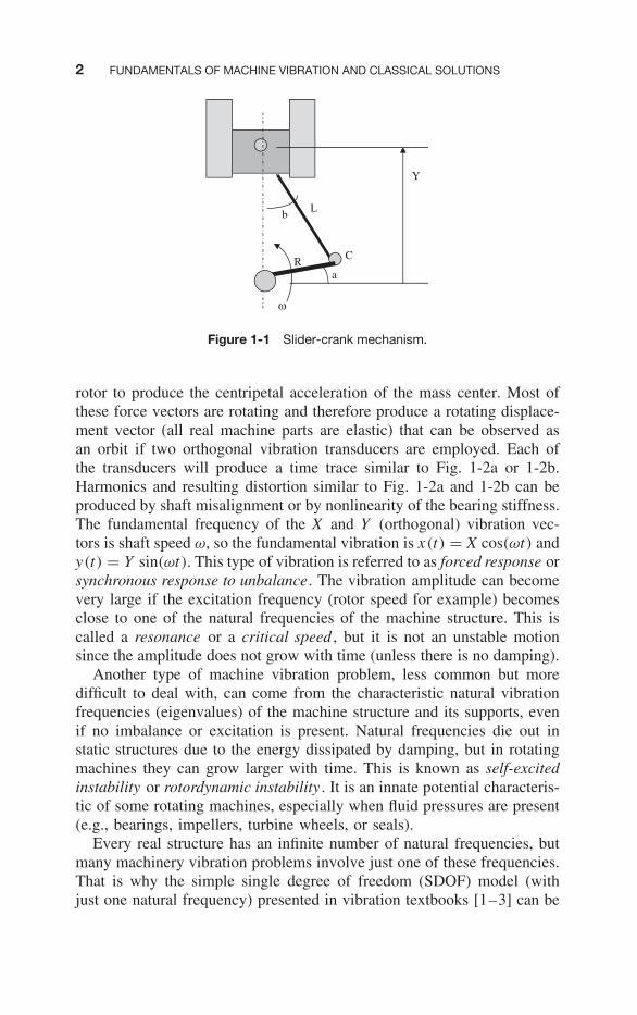
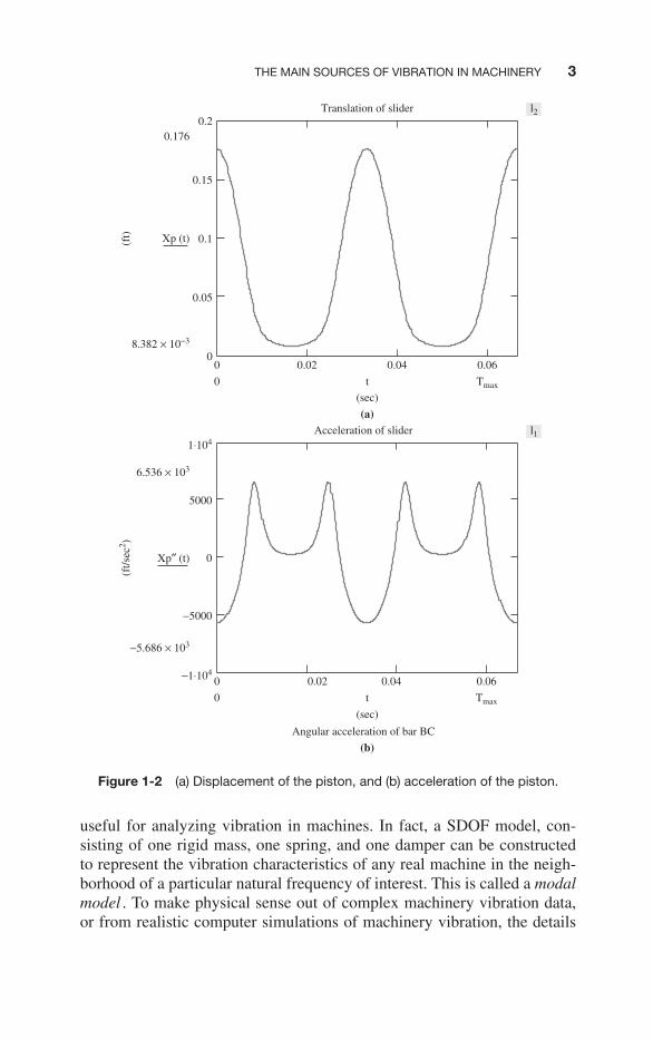
The most common sources of vibration in machinery are related to theinertia of moving parts in the machine. Some parts have a reciprocatingmotion, accelerating back and forth. In such a case Newton’s laws requirea force to accelerate the mass and also require that the force be reacted tothe frame of the machine. The forces are usually periodic and thereforeproduce periodic displacements observed as vibration. For example, thepiston motion in the slider-crank mechanism of Fig. 1-1 has a fundamentalfrequency equal to the crankshaft speed but also has higher frequencies(harmonics). The dominant harmonic is twice crankshaft speed (2nd har-monic). Figure 1-2a shows the displacement of the piston. It looks almostlike a sine wave but it is slightly distorted by higher-order harmonicsdue to the nonlinear kinematics of the mechanism. Fig. 1-2b shows theacceleration of the piston, where the 2nd harmonic is amplified sincethe acceleration amplitude is frequency-squared times the displacementamplitude.

Even without reciprocating parts, most machines have rotating shaftsand wheels that cannot be perfectly balanced, so according to Newton’slaws, there must be a rotating force vector at the bearing supports of each

1

COPYRIG

HTED M

ATERIAL

2 FUNDAMENTALS OF MACHINE VIBRATION AND CLASSICAL SOLUTIONS

Y

Lb

RC

a

ω

Figure 1-1 Slider-crank mechanism.

rotor to produce the centripetal acceleration of the mass center. Most ofthese force vectors are rotating and therefore produce a rotating displace-ment vector (all real machine parts are elastic) that can be observed asan orbit if two orthogonal vibration transducers are employed. Each ofthe transducers will produce a time trace similar to Fig. 1-2a or 1-2b.Harmonics and resulting distortion similar to Fig. 1-2a and 1-2b can beproduced by shaft misalignment or by nonlinearity of the bearing stiffness.The fundamental frequency of the X and Y (orthogonal) vibration vec-tors is shaft speed ω, so the fundamental vibration is x(t) = X cos(ωt) andy(t) = Y sin(ωt). This type of vibration is referred to as forced response orsynchronous response to unbalance. The vibration amplitude can becomevery large if the excitation frequency (rotor speed for example) becomesclose to one of the natural frequencies of the machine structure. This iscalled a resonance or a critical speed , but it is not an unstable motionsince the amplitude does not grow with time (unless there is no damping).

Another type of machine vibration problem, less common but moredifficult to deal with, can come from the characteristic natural vibrationfrequencies (eigenvalues) of the machine structure and its supports, evenif no imbalance or excitation is present. Natural frequencies die out instatic structures due to the energy dissipated by damping, but in rotatingmachines they can grow larger with time. This is known as self-excitedinstability or rotordynamic instability . It is an innate potential characteris-tic of some rotating machines, especially when fluid pressures are present(e.g., bearings, impellers, turbine wheels, or seals).

Every real structure has an infinite number of natural frequencies, butmany machinery vibration problems involve just one of these frequencies.That is why the simple single degree of freedom (SDOF) model (withjust one natural frequency) presented in vibration textbooks [1–3] can be

THE MAIN SOURCES OF VIBRATION IN MACHINERY 3

0 0.02 0.04 0.060

0.05

0.1

0.15

0.2Translation of slider

(sec)

(a)

(b)

(sec)

(ft)

0.176

8.382 × 10−3

6.536 × 103

−5.686 × 103

Xp (t)

Xp″ (t)

Tmax0

l2

l1

0 0.02 0.04 0.06

0

5000

1⋅104

−5000

−1⋅104

Acceleration of slider

Angular acceleration of bar BC

(ft/s

ec2 )

Tmax0 t

t

Figure 1-2 (a) Displacement of the piston, and (b) acceleration of the piston.

useful for analyzing vibration in machines. In fact, a SDOF model, con-sisting of one rigid mass, one spring, and one damper can be constructedto represent the vibration characteristics of any real machine in the neigh-borhood of a particular natural frequency of interest. This is called a modalmodel . To make physical sense out of complex machinery vibration data,or from realistic computer simulations of machinery vibration, the details


of the SDOF mathematical model, its variations, and its solutions mustbe burned indelibly into the mind of the vibration engineer.

THE SINGLE DEGREE OF FREEDOM (SDOF) MODEL

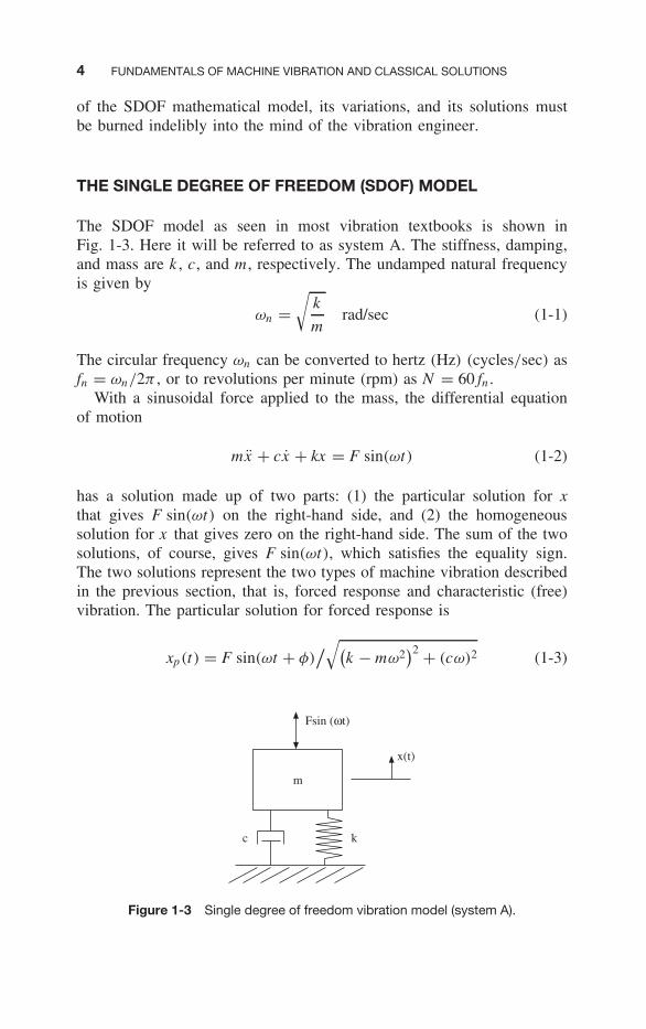
The SDOF model as seen in most vibration textbooks is shown inFig. 1-3. Here it will be referred to as system A. The stiffness, damping,and mass are k , c, and m , respectively. The undamped natural frequencyis given by

ωn =√

k

mrad/sec (1-1)

The circular frequency ωn can be converted to hertz (Hz) (cycles/sec) asfn = ωn/2π , or to revolutions per minute (rpm) as N = 60 fn .

With a sinusoidal force applied to the mass, the differential equationof motion

mx + cx + kx = F sin(ωt) (1-2)

has a solution made up of two parts: (1) the particular solution for xthat gives F sin(ωt) on the right-hand side, and (2) the homogeneoussolution for x that gives zero on the right-hand side. The sum of the twosolutions, of course, gives F sin(ωt), which satisfies the equality sign.The two solutions represent the two types of machine vibration describedin the previous section, that is, forced response and characteristic (free)vibration. The particular solution for forced response is

xp(t) = F sin(ωt + φ)/√(

k − mω2)2 + (cω)2 (1-3)

Fsin (ωt)

m

kc

x(t)

Figure 1-3 Single degree of freedom vibration model (system A).

THE SINGLE DEGREE OF FREEDOM (SDOF) MODEL 5

Notice that the frequency ω of the forced vibration response is the same asthe frequency of the excitation. The angle φ gives the time φ/ω by whichthe response x lags the excitation force F . For analyzing a vibration prob-lem it is important to understand how k , c, and m influence the responseamplitude. They have different effects depending on the frequency ratioω/ωn , as we shall see in the section to follow. Looking at Eq. 1-3 wecan see that the amplitude X of the forced vibration response is

X = F/√(

k − mω2)2 + (cω)2 (1-4)

which depends on k , c, m , ω, and F . Notice that the denominator getssmall when the exciting frequency ω is ωn (Eq. 1-1) unless the dampingcoefficient c is large. A plot of Eq. 1-4 is shown in Fig. 1-7. It is calledthe Bode amplitude plot or the frequency response plot for system A.

The homogeneous part of the solution (for free vibration) with F = 0is given by

xh(t) = Aest (1-5)

where s is a complex number, s = λ + iωd . s is called the eigenvalue.Using the law of exponents, Eq. 1-5 can be rewritten as

xh(t) = Aeλt eiωd t (1-6)

where

eiωd t = cos(ωd t) + i sin(ωd t) (1-7)

Equation 1-5 or 1-6 satisfies the differential Eq. 1-2 with F = 0 providedthat the real part of the eigenvalue is λ = −c/2m and the imaginary partis the square root of ω2

d = k/m − (c/2m)2. The amplitude A in Eq. 1-5is of little interest here since it is determined only by the initial conditionthat instigates the free vibration. In rotating machinery, the differentialequations are more complicated but still are of the same class as (1-2)and have the same form of homogeneous solution as (1-5). The imaginarypart of s , ωd , is the damped natural frequency. Notice that it becomesequal to ωn , Eq. 1-1, when the damping coefficient c = 0.

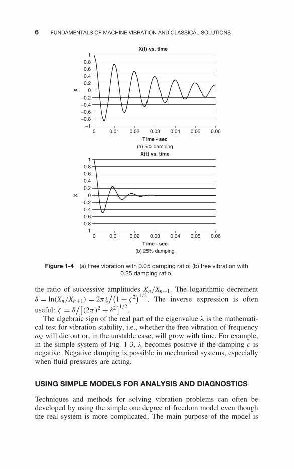
The real part λ of the eigenvalue s determines how fast thefree vibration dies out. It is often converted into a damping ratioζ = c/ccr, where the critical damping ccr = 2mωn . Critical dampingis the amount required to prevent free vibration (and no more). Theconversion equation is ζ = −λ/ωn . Figure 1-4a shows free vibration withζ = 0.05 (5% of critical damping); Fig. 1-4b shows the same systemwith ζ = 0.25 (25% of critical damping). If a free vibration is graphedlike Fig. 1-4, the damping can be expressed as the natural logarithm of


X(t) vs. time

−1−0.8−0.6−0.4−0.2

00.20.40.60.8

1

0 0.01 0.02 0.03 0.04 0.05 0.06

Time - sec

X

(a) 5% damping

(b) 25% damping

X(t) vs. time

−1−0.8−0.6−0.4−0.2

00.20.40.60.8

1

0 0.01 0.02 0.03 0.04 0.05 0.06

Time - sec

X

Figure 1-4 (a) Free vibration with 0.05 damping ratio; (b) free vibration with0.25 damping ratio.

the ratio of successive amplitudes Xn/Xn+1. The logarithmic decrementδ = ln(Xn/Xn+1) = 2πζ

/(1 + ζ 2

)1/2. The inverse expression is often

useful: ζ = δ/[

(2π)2 + δ2]1/2

.The algebraic sign of the real part of the eigenvalue λ is the mathemati-

cal test for vibration stability, i.e., whether the free vibration of frequencyωd will die out or, in the unstable case, will grow with time. For example,in the simple system of Fig. 1-3, λ becomes positive if the damping c isnegative. Negative damping is possible in mechanical systems, especiallywhen fluid pressures are acting.

USING SIMPLE MODELS FOR ANALYSIS AND DIAGNOSTICS

Techniques and methods for solving vibration problems can often bedeveloped by using the simple one degree of freedom model even thoughthe real system is more complicated. The main purpose of the model is

USING SIMPLE MODELS FOR ANALYSIS AND DIAGNOSTICS 7

to provide an understanding of the type of problem being encountered sothat the most effective type of “fix” can be identified. Sometimes a simplemodel can even yield useful approximations for the optimum parametricvalues, such as stiffness and damping to be employed. In contrast to thelarge and detailed finite element models being promoted by some forall diagnostic vibration analysis, this approach suggests that the engineershould first use the simplest possible model that contains the relevantphysical characteristics and resort to the more detailed models only whenthe simple models do not yield sufficient guidance for modifications tothe design or when improved accuracy is desired.

In addition to system A of Fig. 1-3, two more single degree of freedommodels are shown in Figs. 1-5 and 1-6. All three of these systems havea single natural frequency determined by their modal mass and stiffness,but there are subtle differences between the three models that are relatedto the type of excitation.

The constant amplitude exciting force F in system A is generallyunrealistic. Inertia forces in rotating machinery are proportional to speedsquared. Model C in Fig. 1-6 has an unbalanced rotor so that the excitingforce F = mω2u, where u is the offset of the center of rotor mass m fromthe axis of rotation. Note that the mass m is the rotating mass, not thetotal mass, so m on the left side of differential equation (1-2) must bereplaced by the total mass M unless the nonrotating mass is negligible.

In some cases the excitation is a vibration displacement at the base,rather than a force. This is represented by system B in Fig. 1-5.

These small differences in the models produce different frequencyresponse curves. The differences are useful in diagnosing problems anddetermining solutions. Obviously, to use these differences, the engineermust have a complete and thorough knowledge of the three models andtheir responses. The three systems illustrated in Figs. 1-3, 1-5, and 1-6and their mathematical analyses are described in most vibration textbooks[1–3]. In some cases the damping should be included in the most real-istic way possible, i.e., as viscous, Coulomb, hysteretic, or aerodynamicdamping. However, if the damping is other than viscous, it may usually be

Ysin (wt)

m

kc

x(t)

SYSTEM B

Figure 1-5 SDOF model with base excitation.


Rotor mass = m

Total mass = Mkc

x(t)u ωt

SYSTEM C

Unbalance = u

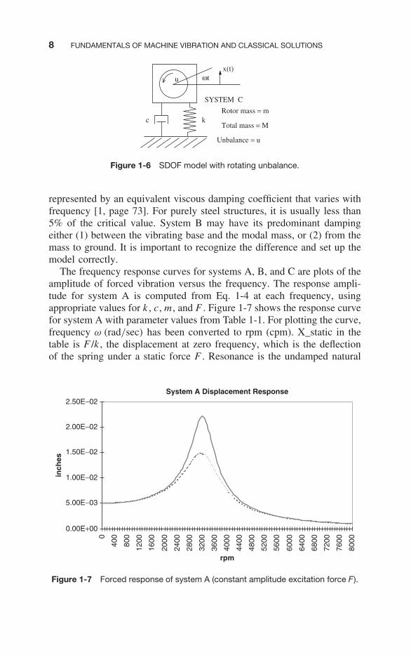
Figure 1-6 SDOF model with rotating unbalance.

represented by an equivalent viscous damping coefficient that varies withfrequency [1, page 73]. For purely steel structures, it is usually less than5% of the critical value. System B may have its predominant dampingeither (1) between the vibrating base and the modal mass, or (2) from themass to ground. It is important to recognize the difference and set up themodel correctly.

The frequency response curves for systems A, B, and C are plots of theamplitude of forced vibration versus the frequency. The response ampli-tude for system A is computed from Eq. 1-4 at each frequency, usingappropriate values for k , c, m , and F . Figure 1-7 shows the response curvefor system A with parameter values from Table 1-1. For plotting the curve,frequency ω (rad/sec) has been converted to rpm (cpm). X_static in thetable is F /k , the displacement at zero frequency, which is the deflectionof the spring under a static force F . Resonance is the undamped natural

System A Displacement Response

0.00E+00

5.00E−03

1.00E−02

1.50E−02

2.00E−02

2.50E−02

0

400

800

1200

1600

2000

2400

2800

3200

3600

4000

4400

4800

5200

5600

6000

6400

6800

7200

7600

8000

rpm

inch

es

Figure 1-7 Forced response of system A (constant amplitude excitation force F).


Table 1-1 System A values for Fig. 1-7

Data Units

InputMass 100 lbKstiff 30,000 lb/inCdamp 20 lb-sec/inForce 150 lbFreqstart 0 rpmFreqstop 8000 rpmNpoints 101 use 101

OutputResonance 3251.252 rpmZeta 0.11349 noneX_static 5.00E-03 in

frequency ωn converted to cpm. Zeta is the critical damping ratio, i.e., thepercentage of critical damping divided by 100. The solid curve in Fig. 1-7has all the parametric values of Table 1-1.

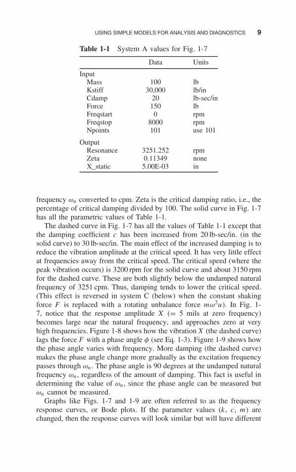
The dashed curve in Fig. 1-7 has all the values of Table 1-1 except thatthe damping coefficient c has been increased from 20 lb-sec/in. (in thesolid curve) to 30 lb-sec/in. The main effect of the increased damping is toreduce the vibration amplitude at the critical speed. It has very little effectat frequencies away from the critical speed. The critical speed (where thepeak vibration occurs) is 3200 rpm for the solid curve and about 3150 rpmfor the dashed curve. These are both slightly below the undamped naturalfrequency of 3251 cpm. Thus, damping tends to lower the critical speed.(This effect is reversed in system C (below) when the constant shakingforce F is replaced with a rotating unbalance force mω2u). In Fig. 1-7, notice that the response amplitude X (= 5 mils at zero frequency)becomes large near the natural frequency, and approaches zero at veryhigh frequencies. Figure 1-8 shows how the vibration X (the dashed curve)lags the force F with a phase angle φ (see Eq. 1-3). Figure 1-9 shows howthe phase angle varies with frequency. More damping (the dashed curve)makes the phase angle change more gradually as the excitation frequencypasses through ωn . The phase angle is 90 degrees at the undamped naturalfrequency ωn , regardless of the amount of damping. This fact is useful indetermining the value of ωn , since the phase angle can be measured butωn cannot be measured.

Graphs like Figs. 1-7 and 1-9 are often referred to as the frequencyresponse curves, or Bode plots. If the parameter values (k , c, m) arechanged, then the response curves will look similar but will have different


X(t) lagging F(t)

−10−8−6−4−202468

10

0 0.02 0.04 0.06 0.08 0.1

Time - sec

F a

nd

X

Figure 1-8 X (dashed) lagging force (solid).

0

30

60

90

120

150

180

0 2000 4000 6000 8000 10000rpm

Deg

rees

Lag

Figure 1-9 Phase lag response of system A.

values of response amplitude and phase. Increasing the damping generallybrings the peak amplitude down but has a negligible effect at frequenciesaway from the natural frequency.

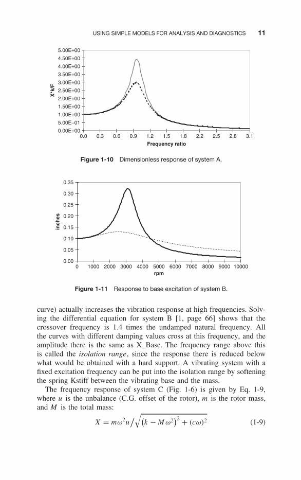
The necessity to plot many different curves for different values of F ,k , and m is avoided by plotting the curve with dimensionless ratios asshown in Fig. 1-10. The abscissa in Fig. 1-10 is frequency ratio ω/ωn ;the ordinate Xk/F is X/X _static (the ratio of vibration amplitude tostatic displacement under the force F ).

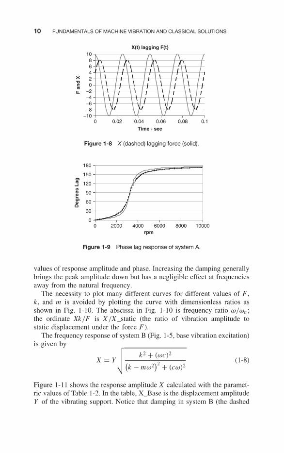
The frequency response of system B (Fig. 1-5, base vibration excitation)is given by

X = Y

√√√√ k2 + (ωc)2(k − mω2

)2 + (cω)2(1-8)

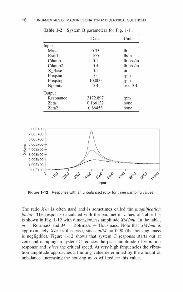
Figure 1-11 shows the response amplitude X calculated with the paramet-ric values of Table 1-2. In the table, X_Base is the displacement amplitudeY of the vibrating support. Notice that damping in system B (the dashed


0.00E+00

5.00E−01

1.00E+00

1.50E+00

2.00E+00

2.50E+00

3.00E+00

3.50E+00

4.00E+00

4.50E+00

5.00E+00

0.0 0.3 0.6 0.9 1.2 1.5 1.8 2.2 2.5 2.8 3.1

Frequency ratio

X*k

/F

Figure 1-10 Dimensionless response of system A.

0.00

0.05

0.10

0.15

0.20

0.25

0.30

0.35

0 1000 2000 3000 4000 5000 6000 7000 8000 9000 10000rpm

inch

es

Figure 1-11 Response to base excitation of system B.

curve) actually increases the vibration response at high frequencies. Solv-ing the differential equation for system B [1, page 66] shows that thecrossover frequency is 1.4 times the undamped natural frequency. Allthe curves with different damping values cross at this frequency, and theamplitude there is the same as X_Base. The frequency range above thisis called the isolation range, since the response there is reduced belowwhat would be obtained with a hard support. A vibrating system with afixed excitation frequency can be put into the isolation range by softeningthe spring Kstiff between the vibrating base and the mass.

The frequency response of system C (Fig. 1-6) is given by Eq. 1-9,where u is the unbalance (C.G. offset of the rotor), m is the rotor mass,and M is the total mass:

X = mω2u/√(

k − M ω2)2 + (cω)2 (1-9)


Table 1-2 System B parameters for Fig. 1-11

Data Units

InputMass 0.35 lbKstiff 100 lb/inCdamp 0.1 lb-sec/inCdamp2 0.4 lb-sec/inX_Base 0.1 inFreqstart 0 rpmFreqstop 10,000 rpmNpoints 101 use 101

OutputResonance 3172.897 rpmZeta 0.166132 noneZeta2 0.66453 none

0.00E+00

1.00E+00

2.00E+00

3.00E+00

4.00E+00

5.00E+00

6.00E+00

7.00E+00

8.00E+00

011

0022

0033

0044

0055

0066

0077

0088

0099

00

1100

0

rpm

XM

/mu

Figure 1-12 Response with an unbalanced rotor for three damping values.

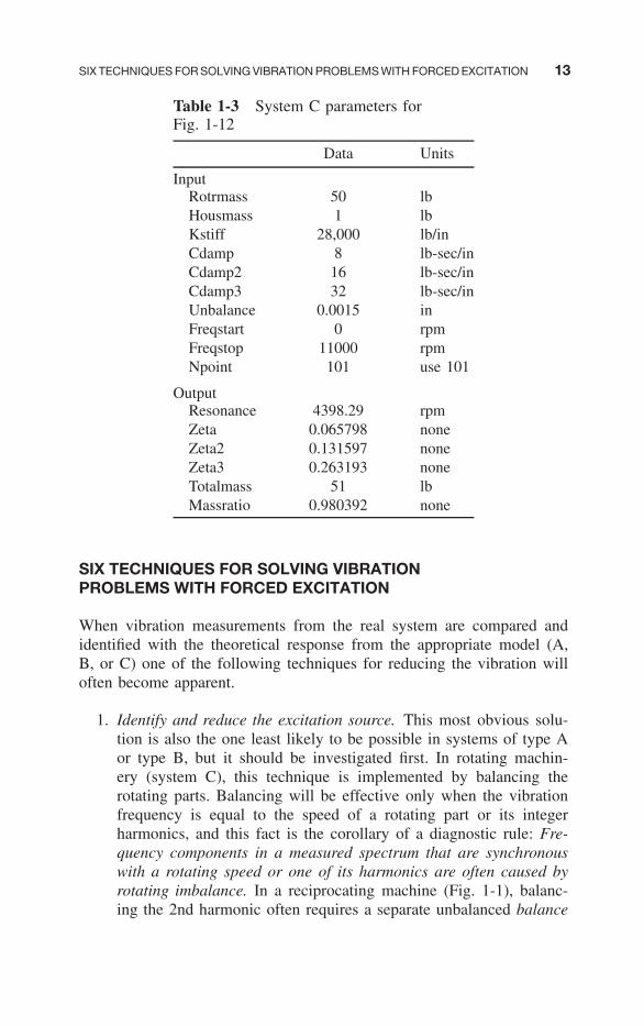
The ratio X /u is often used and is sometimes called the magnificationfactor . The response calculated with the parametric values of Table 1-3is shown in Fig. 1-12 with dimensionless amplitude XM /mu. In the table,m = Rotrmass and M = Rotrmass + Housmass. Note that XM /mu isapproximately X /u in this case, since m/M = 0.98 (the housing massis negligible). Figure 1-12 shows that system C response starts out atzero and damping in system C reduces the peak amplitude of vibrationresponse and raises the critical speed. At very high frequencies the vibra-tion amplitude approaches a limiting value determined by the amount ofunbalance. Increasing the housing mass will reduce this value.

SIX TECHNIQUES FOR SOLVING VIBRATION PROBLEMS WITH FORCED EXCITATION 13

Table 1-3 System C parameters forFig. 1-12

Data Units

InputRotrmass 50 lbHousmass 1 lbKstiff 28,000 lb/inCdamp 8 lb-sec/inCdamp2 16 lb-sec/inCdamp3 32 lb-sec/inUnbalance 0.0015 inFreqstart 0 rpmFreqstop 11000 rpmNpoint 101 use 101

OutputResonance 4398.29 rpmZeta 0.065798 noneZeta2 0.131597 noneZeta3 0.263193 noneTotalmass 51 lbMassratio 0.980392 none

SIX TECHNIQUES FOR SOLVING VIBRATIONPROBLEMS WITH FORCED EXCITATION

When vibration measurements from the real system are compared andidentified with the theoretical response from the appropriate model (A,B, or C) one of the following techniques for reducing the vibration willoften become apparent.

1. Identify and reduce the excitation source. This most obvious solu-tion is also the one least likely to be possible in systems of type Aor type B, but it should be investigated first. In rotating machin-ery (system C), this technique is implemented by balancing therotating parts. Balancing will be effective only when the vibrationfrequency is equal to the speed of a rotating part or its integerharmonics, and this fact is the corollary of a diagnostic rule: Fre-quency components in a measured spectrum that are synchronouswith a rotating speed or one of its harmonics are often caused byrotating imbalance. In a reciprocating machine (Fig. 1-1), balanc-ing the 2nd harmonic often requires a separate unbalanced balance


shaft rotating at twice crankshaft speed to cancel out the inertiaforces.

2. Tune the natural frequency to a value further away from the frequencyof excitation to avoid resonance. A study of the frequency responsecurves for any of the systems A, B, or C reveals that the vibra-tory excitation is highly magnified at frequencies near the naturalfrequency. This magnification factor R, or Q factor as it is some-times called, can typically range from 5 to 50 or more dependingon the amount of damping. The excitation frequency can seldom bechanged, but the natural frequency can sometimes be easily changedby changing the modal stiffness. This is one place where intelligentconstruction of the analytical model becomes important, since themodal stiffness may be made up of several real stiffnesses in par-allel or in series. In parallel combinations the very low stiffnesseshave little effect in determining the modal stiffness, while in seriescombinations the very high stiffnesses have little effect. The tuningmethod is effective only when the excitation frequency is constantor when it only varies over a narrow range.

3. Isolate the modal mass from the vibratory excitation by making themodal stiffness very low. Notice that all the response curves showa very low response to the vibratory excitation at frequencies muchhigher than the natural frequency (far to the right on the responsecurves). Once again, the excitation frequency usually cannot bechanged but the natural frequency can be brought far down by avery soft modal stiffness, thus placing the system response far tothe right of resonance on the response curve. This method is par-ticularly effective in systems of type B. A typical application isisolating an electronics box from a vibrating vehicle frame.

4. Add damping to the system. Damping is added by incorporatingmechanisms that dissipate vibratory energy into heat. When theywork, damping mechanisms produce forces that act in opposition tothe vibratory velocity. Contrary to popular belief, however, addingdamping indiscriminately does not always reduce vibration. Damp-ing does work well whenever operation is near resonance (and thisis the operating condition most likely to cause a problem). At fre-quencies away from resonance damping has very little effect, exceptto increase the forces transmitted to ground at high frequencies farabove resonance. In a system B application where isolation is used,damping added between the modal mass and the vibrating supportwill actually increase the vibration of the mass at high frequencies.In a system C (rotating machinery) application with rolling elementbearings, adding damping to the bearing supports will increase the

SOME EXAMPLES WITH FORCED EXCITATION 15

dynamic bearing loads and shorten bearing life for operation at highsupercritical speeds [4, page 14].

5. Add a vibration absorber. A vibration absorber is a separatespring–mass assembly, which is added to the original system to“absorb” the vibration. This method works well only under a strictset of conditions: (a) the excitation frequency must be constantand resonant (i.e., equal to a natural frequency of the system), (b)the absorber spring–mass assembly must be tuned to a naturalfrequency equal to the resonant frequency of the original system, (c)the absorber mass should be at least 20 percent of the modal massof the original system, and (d) the absorber spring–mass assemblyshould not have much damping. Under all of these conditionsthe modal mass of the original system will stand still while theabsorber mass vibrates with a large amplitude. Since the absorberadds a degree of freedom to the analytical model, it follows thatmathematical analysis of absorber performance requires at least atwo degree of freedom model with two differential equations tosolve simultaneously [2, page 293].

6. Stiffen the system. This method is listed last because it is valid onlyfor systems of type A, but often is mistakenly suggested for alltype systems. On the dimensionless response curves for system A(Fig. 1-10), notice on the vertical amplitude axis that the vibrationamplitude X is determined by multiplying the graph value by F /k .Thus, the vibration amplitude can be made smaller at any frequencyby raising the stiffness k . Once again, this applies only to systemsof type A in which there is a constant amplitude force excitationthat does not vary with frequency.

SOME EXAMPLES WITH FORCED EXCITATION

Illustrative Example 1

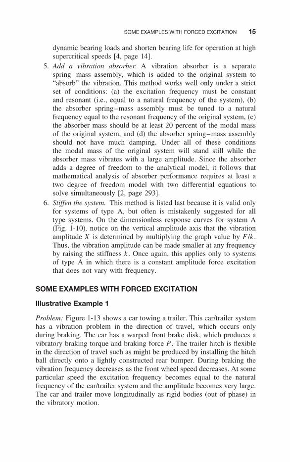
Problem: Figure 1-13 shows a car towing a trailer. This car/trailer systemhas a vibration problem in the direction of travel, which occurs onlyduring braking. The car has a warped front brake disk, which produces avibratory braking torque and braking force P . The trailer hitch is flexiblein the direction of travel such as might be produced by installing the hitchball directly onto a lightly constructed rear bumper. During braking thevibration frequency decreases as the front wheel speed decreases. At someparticular speed the excitation frequency becomes equal to the naturalfrequency of the car/trailer system and the amplitude becomes very large.The car and trailer move longitudinally as rigid bodies (out of phase) inthe vibratory motion.


Analysis: Let the car displacement be X1 and the trailer be X2 (relativeto the displacement produced by travel speed). There are two degrees offreedom (dof), but the system can be reduced to 1 dof because there is nospring to ground. The two differential equations (one for each dof) can becombined by subtracting one from the other (because the first mode haszero frequency). X = X1 − X2 is a modal coordinate. This produces thesystem A differential equation (1-2), where me is the modal or equivalentmass and Pe is the modal or equivalent force as follows:

meX + KX = Pe (1-10)

whereme = m1m2

m1 + m2(1-11)

Pe = m2P

m1 + m2(1-12)

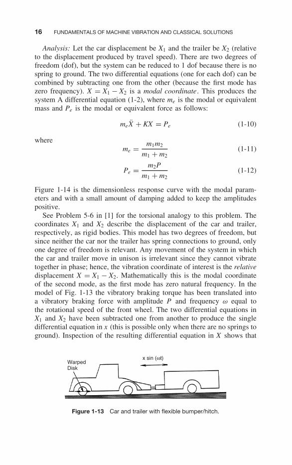
Figure 1-14 is the dimensionless response curve with the modal param-eters and with a small amount of damping added to keep the amplitudespositive.

See Problem 5-6 in [1] for the torsional analogy to this problem. Thecoordinates X1 and X2 describe the displacement of the car and trailer,respectively, as rigid bodies. This model has two degrees of freedom, butsince neither the car nor the trailer has spring connections to ground, onlyone degree of freedom is relevant. Any movement of the system in whichthe car and trailer move in unison is irrelevant since they cannot vibratetogether in phase; hence, the vibration coordinate of interest is the relativedisplacement X = X1 − X2. Mathematically this is the modal coordinateof the second mode, as the first mode has zero natural frequency. In themodel of Fig. 1-13 the vibratory braking torque has been translated intoa vibratory braking force with amplitude P and frequency ω equal tothe rotational speed of the front wheel. The two differential equations inX1 and X2 have been subtracted one from another to produce the singledifferential equation in x (this is possible only when there are no springs toground). Inspection of the resulting differential equation in X shows that

WarpedDisk

x sin (ωt)

Figure 1-13 Car and trailer with flexible bumper/hitch.


0

5

10

15

20

25

30

0 0.2 0.4 0.6 0.8 1 1.2 1.4 1.6omega/omega_n

KX

/Pe

Figure 1-14 Dimensionless response of the car and trailer to the warpedbrake disk.

the modal mass me is m1m2(m1 + m2) and the equivalent excitation forcePe is Pm2/(m1 + m2). The modal stiffness is simply the hitch connectionstiffness K . The system is of Type A since the differential equation hasexactly the same form as the system A equation 1–2 . This is true becausethe equivalent excitation is a constant force F = Pe . Notice that the modalmass can be easily calculated from the weights of the car and trailer,and the modal stiffness K can be measured directly by applying staticforces to the hitch or by measuring the resonant frequency and calculatingK = ω2me . The numerical magnitude of P need not be known to arriveat useful solutions as will be seen below.

Solution: Consider the six different methods described above for reduc-ing vibration. The first method, reducing the source, could be implementedby replacing the warped brake disk and would be the ideal solution. Iffor some reason this cannot be done, consider the remaining methods.Tuning or absorption will not work because the excitation frequency isvariable. Isolation will not work because the excitation frequency goes allthe way down to zero. Damping would help at frequencies near resonance,but requires the addition of an expensive damping element to the flexiblehitch connection at the rear bumper. Method 6, stiffening the system, canbe implemented by stiffening the rear bumper or hitch connection andwould be the best approach if the warped brake disk cannot be correctedor replaced. On the dimensionless response curve, note the effect of K onthe value of X at every frequency. Stiffening the system in this case willreduce the response at all frequencies.


Problem: It is desired to mount an electronics package onto a vibratingsurface with assurance that the electronics will survive. This generallyrequires that testing be done to define the limits of the vibratory envi-ronment that could damage the electronics in the package and also that


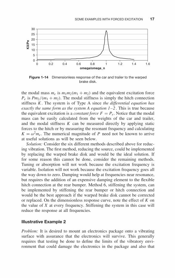
the vibration amplitude of the mounting surface be known as a functionof frequency (preferably from testing). In this example an electronic boxweighing 0.35 lb is to be supported on a bracket that is welded to a vibrat-ing bulkhead (Fig. 1-15). The excitation is rotating unbalance. A rubbermounting pad is to be designed as a vibration isolator. The vibration lim-its specified by the electronics manufacturer are shown in Fig. 1-16. Thebulkhead vibration measured with an accelerometer is shown in Fig. 1-17.

Analysis: This type of problem is almost always addressed with method3 (isolation) and is modeled by system B. It is helpful to plot the sys-tem B response curve in terms of dimensionless parameters as shown inFig. 1-18. The frequency ratio is the ratio of the exciting frequency ω tothe undamped natural frequency ωn .

2"

H

3"

u (t )1" 4

Figure 1-15 Electronic box installation.

Safe

Vibration limits for electronic box

Frequency - Hz

−1.63g

4.88g

100

1

2

3

4

5

200 300

A

g

Figure 1-16 Vibration limits for the electronics.


Housing vibration amplitude

Frequency - Hz850.0

0

1

2

3

4

5

6

7

170 255 340

A

g

Figure 1-17 Measured bulkhead vibration, g’s.

0.00E+00

5.00E−01

1.00E+00

1.50E+00

2.00E+00

2.50E+00

3.00E+00

3.50E+00

0.00 0.32 0.63 0.95 1.26 1.58 1.89 2.21 2.52 2.84 3.15

Frequency Ratio

X/Y

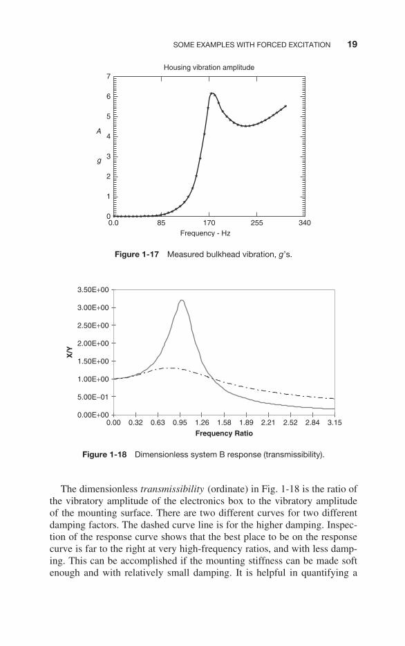
Figure 1-18 Dimensionless system B response (transmissibility).

The dimensionless transmissibility (ordinate) in Fig. 1-18 is the ratio ofthe vibratory amplitude of the electronics box to the vibratory amplitudeof the mounting surface. There are two different curves for two differentdamping factors. The dashed curve line is for the higher damping. Inspec-tion of the response curve shows that the best place to be on the responsecurve is far to the right at very high-frequency ratios, and with less damp-ing. This can be accomplished if the mounting stiffness can be made softenough and with relatively small damping. It is helpful in quantifying a


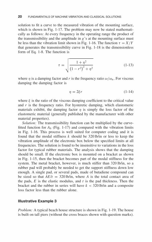
solution to fit a curve to the measured vibration of the mounting surface,which is shown in Fig. 1-17. The problem may now be stated mathemati-cally as follows: At every frequency in the operating range the product ofthe transmissibility and the amplitude in g’s at the mounting surface mustbe less than the vibration limit shown in Fig. 1-16. The function τ = X/Ythat generates the transmissibility curve in Fig. 1-18 is the dimensionlessform of Eq. 1-8. The function is

τ =√√√√ 1 + η2(

1 − r2)2 + η2

(1-13)

where η is a damping factor and r is the frequency ratio ω/ωn . For viscousdamping the damping factor is

η = 2ξr (1-14)

where ξ is the ratio of the viscous damping coefficient to the critical valueand r is the frequency ratio. For hysteretic damping, which elastomericmaterials exhibit, the damping factor η is simply the loss factor of theelastomeric material (generally published by the manufacturer with othermaterial properties).

Solution: The transmissibility function can be multiplied by the curve-fitted function for Ab (Fig. 1-17) and compared with the vibration limitsin Fig. 1-16. This process is well suited for computer coding and it isfound that the modal stiffness k should be 320 lb/in or less to keep thevibration amplitude of the electronic box below the specified limits at allfrequencies. The solution is found to be insensitive to variations in the lossfactor for typical rubber materials. The analysis shows that the dampingshould be small. If the electronic box is mounted on a bracket as shownin Fig. 1-15, then the bracket becomes part of the modal stiffness for thesystem. The metal bracket, however, is much stiffer than 320 lb/in, so arubber pad will probably be needed to get the support stiffness down lowenough. A single pad, or several pads, made of butadiene compound canbe sized so that AE /t = 320 lb/in, where A is the total contact area ofthe pads, E is the elastic modulus, and t is the pad thickness. Then thebracket and the rubber in series will have k < 320 lb/in and a compositeloss factor less than the rubber alone.


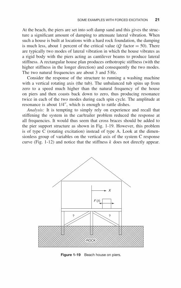
Problem: A typical beach house structure is shown in Fig. 1-19. The houseis built on tall piers (without the cross braces shown with question marks).


At the beach, the piers are set into soft damp sand and this gives the struc-ture a significant amount of damping to attenuate lateral vibration. Whensuch a house is built at locations with a hard rock foundation, the dampingis much less, about 1 percent of the critical value (Q factor = 50). Thereare typically two modes of lateral vibration in which the house vibrates asa rigid body with the piers acting as cantilever beams to produce lateralstiffness. A rectangular house plan produces orthotropic stiffness (with thehigher stiffness in the longer direction) and consequently the two modes.The two natural frequencies are about 3 and 5 Hz.

Consider the response of the structure to running a washing machinewith a vertical rotating axis (the tub). The unbalanced tub spins up fromzero to a speed much higher than the natural frequency of the houseon piers and then coasts back down to zero, thus producing resonancetwice in each of the two modes during each spin cycle. The amplitude atresonance is about 1/4′′, which is enough to rattle dishes.

Analysis: It is tempting to simply rely on experience and recall thatstiffening the system in the car/trailer problem reduced the response atall frequencies. It would thus seem that cross braces should be added tothe pier support structure as shown in Fig. 1-19. However, this problemis of type C (rotating excitation) instead of type A. Look at the dimen-sionless group of variables on the vertical axis of the system C responsecurve (Fig. 1-12) and notice that the stiffness k does not directly appear.

F (t )

X

??

ROCK

Figure 1-19 Beach house on piers.


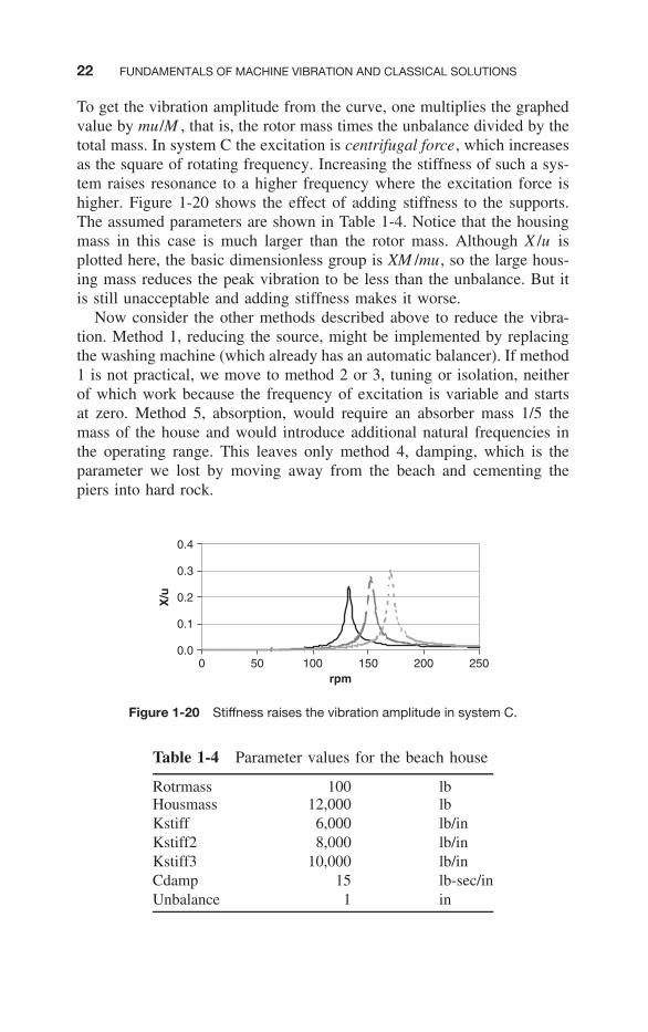
To get the vibration amplitude from the curve, one multiplies the graphedvalue by mu/M , that is, the rotor mass times the unbalance divided by thetotal mass. In system C the excitation is centrifugal force, which increasesas the square of rotating frequency. Increasing the stiffness of such a sys-tem raises resonance to a higher frequency where the excitation force ishigher. Figure 1-20 shows the effect of adding stiffness to the supports.The assumed parameters are shown in Table 1-4. Notice that the housingmass in this case is much larger than the rotor mass. Although X /u isplotted here, the basic dimensionless group is XM /mu, so the large hous-ing mass reduces the peak vibration to be less than the unbalance. But itis still unacceptable and adding stiffness makes it worse.

Now consider the other methods described above to reduce the vibra-tion. Method 1, reducing the source, might be implemented by replacingthe washing machine (which already has an automatic balancer). If method1 is not practical, we move to method 2 or 3, tuning or isolation, neitherof which work because the frequency of excitation is variable and startsat zero. Method 5, absorption, would require an absorber mass 1/5 themass of the house and would introduce additional natural frequencies inthe operating range. This leaves only method 4, damping, which is theparameter we lost by moving away from the beach and cementing thepiers into hard rock.

0.0

0.1

0.2

0.3

0.4

0 50 100 150 200 250rpm

X/u

Figure 1-20 Stiffness raises the vibration amplitude in system C.

Table 1-4 Parameter values for the beach house

Rotrmass 100 lbHousmass 12,000 lbKstiff 6,000 lb/inKstiff2 8,000 lb/inKstiff3 10,000 lb/inCdamp 15 lb-sec/inUnbalance 1 in


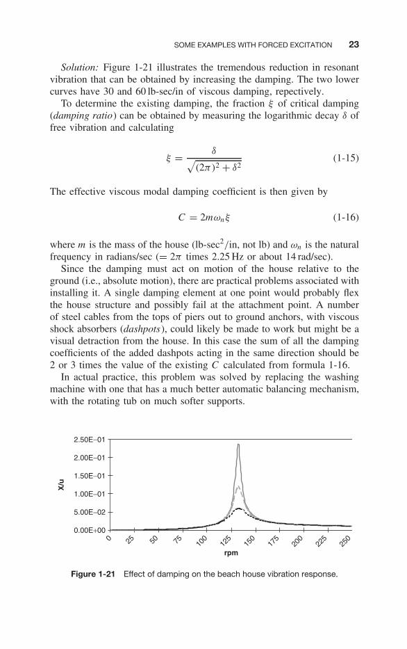
Solution: Figure 1-21 illustrates the tremendous reduction in resonantvibration that can be obtained by increasing the damping. The two lowercurves have 30 and 60 lb-sec/in of viscous damping, repectively.

To determine the existing damping, the fraction ξ of critical damping(damping ratio) can be obtained by measuring the logarithmic decay δ offree vibration and calculating

ξ = δ√(2π)2 + δ2

(1-15)

The effective viscous modal damping coefficient is then given by

C = 2mωnξ (1-16)

where m is the mass of the house (lb-sec2/in, not lb) and ωn is the naturalfrequency in radians/sec (= 2π times 2.25 Hz or about 14 rad/sec).

Since the damping must act on motion of the house relative to theground (i.e., absolute motion), there are practical problems associated withinstalling it. A single damping element at one point would probably flexthe house structure and possibly fail at the attachment point. A numberof steel cables from the tops of piers out to ground anchors, with viscousshock absorbers (dashpots), could likely be made to work but might be avisual detraction from the house. In this case the sum of all the dampingcoefficients of the added dashpots acting in the same direction should be2 or 3 times the value of the existing C calculated from formula 1-16.

In actual practice, this problem was solved by replacing the washingmachine with one that has a much better automatic balancing mechanism,with the rotating tub on much softer supports.

0.00E+00

5.00E−02

1.00E−01

1.50E−01

2.00E−01

2.50E−01

0 25 50 75 100

125

150

175

200

225

250

rpm

X/u

Figure 1-21 Effect of damping on the beach house vibration response.



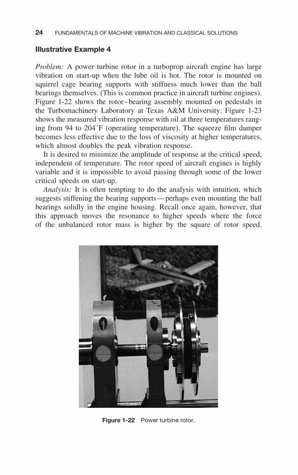
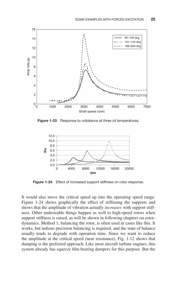
Problem: A power turbine rotor in a turboprop aircraft engine has largevibration on start-up when the lube oil is hot. The rotor is mounted onsquirrel cage bearing supports with stiffness much lower than the ballbearings themselves. (This is common practice in aircraft turbine engines).Figure 1-22 shows the rotor–bearing assembly mounted on pedestals inthe Turbomachinery Laboratory at Texas A&M University. Figure 1-23shows the measured vibration response with oil at three temperatures rang-ing from 94 to 204◦F (operating temperature). The squeeze film damperbecomes less effective due to the loss of viscosity at higher temperatures,which almost doubles the peak vibration response.

It is desired to minimize the amplitude of response at the critical speed,independent of temperature. The rotor speed of aircraft engines is highlyvariable and it is impossible to avoid passing through some of the lowercritical speeds on start-up.

Analysis: It is often tempting to do the analysis with intuition, whichsuggests stiffening the bearing supports—perhaps even mounting the ballbearings solidly in the engine housing. Recall once again, however, thatthis approach moves the resonance to higher speeds where the forceof the unbalanced rotor mass is higher by the square of rotor speed.

Figure 1-22 Power turbine rotor.


94–109 deg

141–144 deg

199–204 deg

00

2

4

6

8

10

12

14

16

1000 2000 3000 4000 5000 6000 7000

Shaft speed (rpm)

Am

p m

ils-p

p

Figure 1-23 Response to unbalance at three oil temperatures.

0.0

2.0

4.0

6.0

8.0

10.0

12.0

0 4000 8000 12000 16000 20000rpm

X/u

Figure 1-24 Effect of increased support stiffness on rotor response.

It would also move the critical speed up into the operating speed range.Figure 1-24 shows graphically the effect of stiffening the supports andshows that the amplitude of vibration actually increases with support stiff-ness. Other undesirable things happen as well to high-speed rotors whensupport stiffness is raised, as will be shown in following chapters on rotor-dynamics. Method 1, balancing the rotor, is often used in cases like this. Itworks, but tedious precision balancing is required, and the state of balanceusually tends to degrade with operation time. Since we want to reducethe amplitude at the critical speed (near resonance), Fig. 1-12 shows thatdamping is the preferred approach. Like most aircraft turbine engines, thissystem already has squeeze film bearing dampers for this purpose. But the


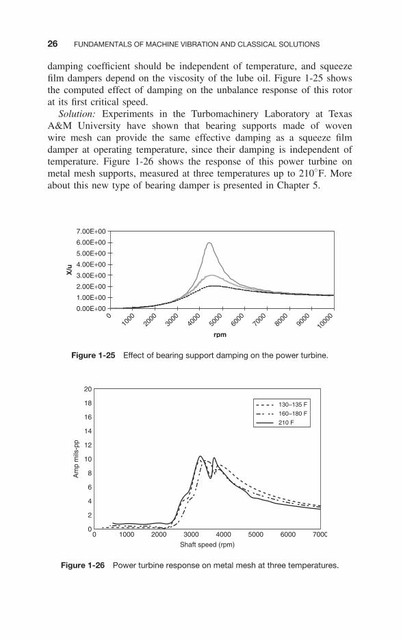
damping coefficient should be independent of temperature, and squeezefilm dampers depend on the viscosity of the lube oil. Figure 1-25 showsthe computed effect of damping on the unbalance response of this rotorat its first critical speed.

Solution: Experiments in the Turbomachinery Laboratory at TexasA&M University have shown that bearing supports made of wovenwire mesh can provide the same effective damping as a squeeze filmdamper at operating temperature, since their damping is independent oftemperature. Figure 1-26 shows the response of this power turbine onmetal mesh supports, measured at three temperatures up to 210◦F. Moreabout this new type of bearing damper is presented in Chapter 5.

0.00E+00

1.00E+00

2.00E+00

3.00E+00

4.00E+00

5.00E+00

6.00E+00

7.00E+00

010

0020

0030

0040

0050

0060

0070

0080

0090

00

1000

0

rpm

X/u

Figure 1-25 Effect of bearing support damping on the power turbine.

130–135 F

160–180 F

210 F

00

2

4

6

8

10

12

14

16

18

20

1000 2000 3000

Shaft speed (rpm)

Am

p m

ils-p

p

4000 5000 6000 7000

Figure 1-26 Power turbine response on metal mesh at three temperatures.

SOME OBSERVATIONS ABOUT MODELING 27

SOME OBSERVATIONS ABOUT MODELING

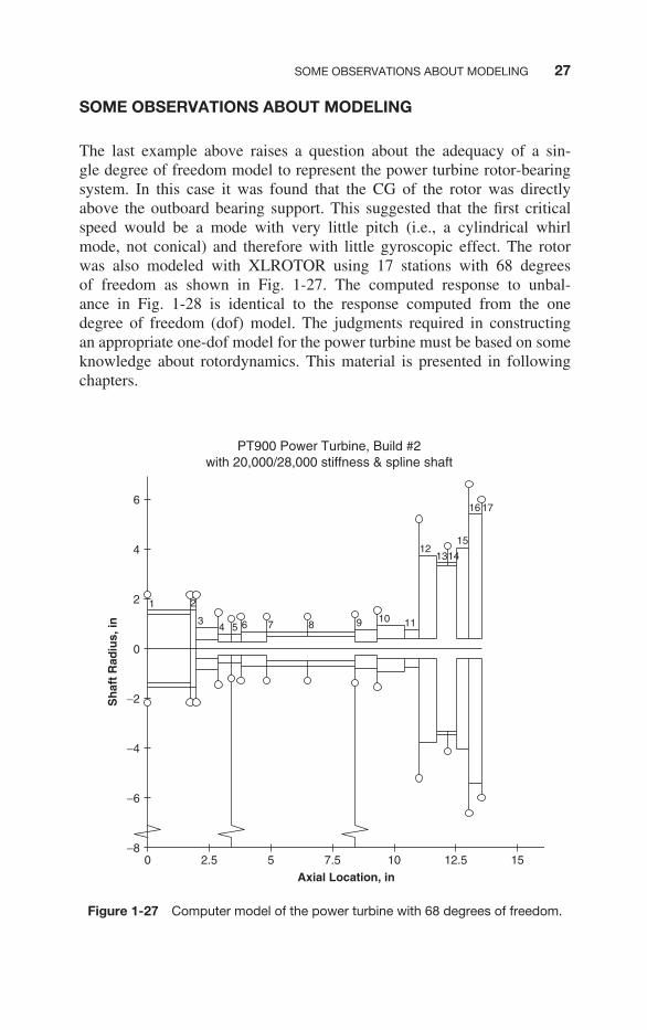
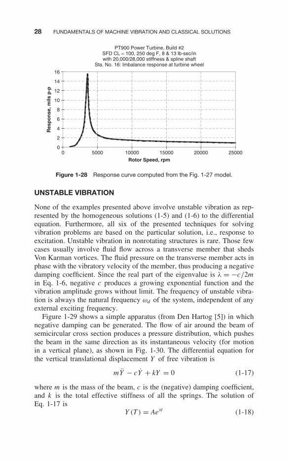
The last example above raises a question about the adequacy of a sin-gle degree of freedom model to represent the power turbine rotor-bearingsystem. In this case it was found that the CG of the rotor was directlyabove the outboard bearing support. This suggested that the first criticalspeed would be a mode with very little pitch (i.e., a cylindrical whirlmode, not conical) and therefore with little gyroscopic effect. The rotorwas also modeled with XLROTOR using 17 stations with 68 degreesof freedom as shown in Fig. 1-27. The computed response to unbal-ance in Fig. 1-28 is identical to the response computed from the onedegree of freedom (dof) model. The judgments required in constructingan appropriate one-dof model for the power turbine must be based on someknowledge about rotordynamics. This material is presented in followingchapters.

1716

15

141312

11109876543

21

−8

−6

−4

−2

0

2

4

6

0 2.5 7.55 10 12.5 15

Axial Location, in

Sh

aft

Rad

ius,

in

PT900 Power Turbine, Build #2with 20,000/28,000 stiffness & spline shaft

Figure 1-27 Computer model of the power turbine with 68 degrees of freedom.


0

2

4

6

8

10

12

14

16

0 5000 10000 15000 20000 25000

Rotor Speed, rpm

Res

po

nse

, mils

p-p

PT900 Power Turbine, Build #2SFD CL = 100, 250 deg F, 8 & 13 lb-sec/inwith 20,000/28,000 stiffness & spline shaft

Sta. No. 16: Imbalance response at turbine wheel

Figure 1-28 Response curve computed from the Fig. 1-27 model.

UNSTABLE VIBRATION

None of the examples presented above involve unstable vibration as rep-resented by the homogeneous solutions (1-5) and (1-6) to the differentialequation. Furthermore, all six of the presented techniques for solvingvibration problems are based on the particular solution, i.e., response toexcitation. Unstable vibration in nonrotating structures is rare. Those fewcases usually involve fluid flow across a transverse member that shedsVon Karman vortices. The fluid pressure on the transverse member acts inphase with the vibratory velocity of the member, thus producing a negativedamping coefficient. Since the real part of the eigenvalue is λ = −c/2min Eq. 1-6, negative c produces a growing exponential function and thevibration amplitude grows without limit. The frequency of unstable vibra-tion is always the natural frequency ωd of the system, independent of anyexternal exciting frequency.

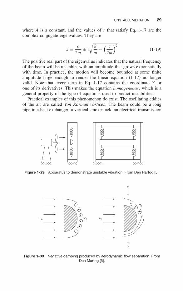
Figure 1-29 shows a simple apparatus (from Den Hartog [5]) in whichnegative damping can be generated. The flow of air around the beam ofsemicircular cross section produces a pressure distribution, which pushesthe beam in the same direction as its instantaneous velocity (for motionin a vertical plane), as shown in Fig. 1-30. The differential equation forthe vertical translational displacement Y of free vibration is

mY − cY + kY = 0 (1-17)

where m is the mass of the beam, c is the (negative) damping coefficient,and k is the total effective stiffness of all the springs. The solution ofEq. 1-17 is

Y (T ) = Aest (1-18)

UNSTABLE VIBRATION 29

where A is a constant, and the values of s that satisfy Eq. 1-17 are thecomplex conjugate eigenvalues. They are

s = c

2m± i

√k

m−

( c

2m

)2(1-19)

The positive real part of the eigenvalue indicates that the natural frequencyof the beam will be unstable, with an amplitude that grows exponentiallywith time. In practice, the motion will become bounded at some finiteamplitude large enough to render the linear equation (1-17) no longervalid. Note that every term in Eq. 1-17 contains the coordinate Y orone of its derivatives. This makes the equation homogeneous , which is ageneral property of the type of equations used to predict instabilities.

Practical examples of this phenomenon do exist. The oscillating eddiesof the air are called Von Karman vortices . The beam could be a longpipe in a heat exchanger, a vertical smokestack, an electrical transmission

Figure 1-29 Apparatus to demonstrate unstable vibration. From Den Hartog [5].

u0 u0P0

P0

Y

F

Figure 1-30 Negative damping produced by aerodynamic flow separation. FromDen Martog [5].


wire, or a guy wire. However, unstable vibration is much more commonin rotating machinery than in structures and can be very destructive. Inrotating machinery it is called rotordynamic instability . It is generallycaused by cross-coupled stiffness instead of negative direct damping. Itwill be analyzed and discussed in chapters to follow.

REFERENCES

[1] Thomson, W. T. Theory of Vibration with Applications , 4th ed. EnglewoodCliffs, NJ: Prentice Hall, 1993.

[2] Steidel, R. F., Jr. An Introduction to Mechanical Vibrations . New York:Wiley, 1989.

[3] Den Hartog, J. P. Mechanical Vibrations , 4th ed. New York: McGraw-Hill,1956.

[4] Vance, J. M. Rotordynamics of Turbomachinery . New York: Wiley, 1988.[5] Den Hartog, J. P. Mechanical Vibration, 4th ed. New York: McGraw-Hill,

1956, p. 301.

EXERCISES

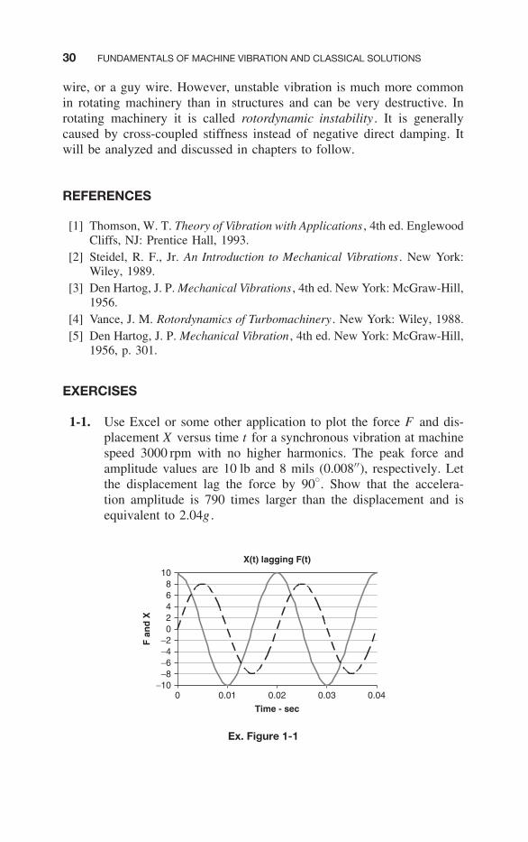
1-1. Use Excel or some other application to plot the force F and dis-placement X versus time t for a synchronous vibration at machinespeed 3000 rpm with no higher harmonics. The peak force andamplitude values are 10 lb and 8 mils (0.008′′), respectively. Letthe displacement lag the force by 90◦. Show that the accelera-tion amplitude is 790 times larger than the displacement and isequivalent to 2.04g .

X(t) lagging F(t)

−10−8−6−4−202468

10

0 0.01 0.02 0.03 0.04

Time - sec

F a

nd

X

Ex. Figure 1-1

EXERCISES 31

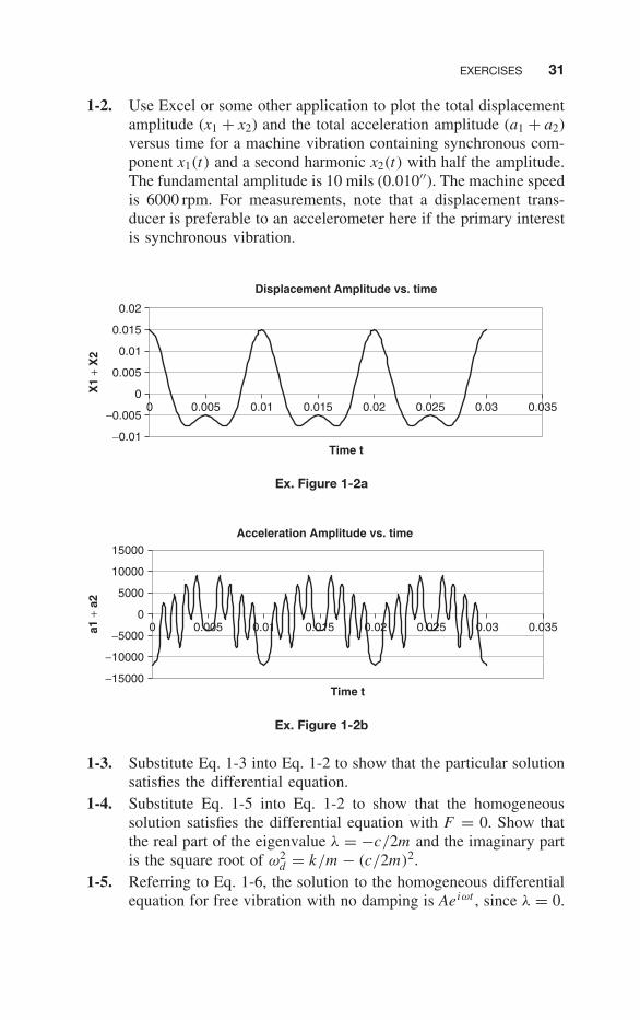
1-2. Use Excel or some other application to plot the total displacementamplitude (x1 + x2) and the total acceleration amplitude (a1 + a2)versus time for a machine vibration containing synchronous com-ponent x1(t) and a second harmonic x2(t) with half the amplitude.The fundamental amplitude is 10 mils (0.010′′). The machine speedis 6000 rpm. For measurements, note that a displacement trans-ducer is preferable to an accelerometer here if the primary interestis synchronous vibration.

Displacement Amplitude vs. time

−0.01

−0.005

0

0.005

0.01

0.015

0.02

0 0.005 0.01 0.015 0.02 0.025 0.03 0.035

Time t

X1

+ X

2

Ex. Figure 1-2a

Acceleration Amplitude vs. time

−15000

−10000

−5000

0

5000

10000

15000

0 0.005 0.01 0.015 0.02 0.025 0.03 0.035

Time t

a1 +

a2

Ex. Figure 1-2b

1-3. Substitute Eq. 1-3 into Eq. 1-2 to show that the particular solutionsatisfies the differential equation.

1-4. Substitute Eq. 1-5 into Eq. 1-2 to show that the homogeneoussolution satisfies the differential equation with F = 0. Show thatthe real part of the eigenvalue λ = −c/2m and the imaginary partis the square root of ω2

d = k/m − (c/2m)2.1-5. Referring to Eq. 1-6, the solution to the homogeneous differential

equation for free vibration with no damping is Aeiωt , since λ = 0.


Show that the solution can also can be written as A1 cos(ωn t) +A2 sin(ωn t), where A1 and A2 are real numbers and ωn = (k/m)1/2,provided that A is an arbitrary complex number.

1-6. Show that eq. 1-6 with nonzero damping can be expressed

as xh(t) = e− c2m t [A1 cos(ωd t) + A2 sin(ωd t)]. Assuming ini-

tial conditions to give A2 = 0, take the ratio of successiveamplitudes Xn/Xn+1 to show that the logarithmic decrementδ = ln(Xn/Xn+1) = 2πζ/

(1 + ζ 2

)1/2, where ζ = c/2mωn .

Hint: Note that the period of the damped vibration is 2π/ωd .1-7. The tuning method on page 14 states that intelligent construction

of the analytical model is important, since the modal stiffness maybe made up of several real stiffnesses in parallel or in series. Inparallel combinations the very low stiffnesses have little effect indetermining the modal stiffness, while in series combinations thevery high stiffnesses have little effect.

a. Show that the effective stiffness of k1 and k2 in parallel ispractically k1 if k1 = 100k2.

b. Show that the effective stiffness of k1 and k2 in series is prac-tically k2 if k1 = 100k2.

1-8. Derive the dimensionless form of Eq. 1-3 for the purpose of plot-ting Fig. 1-14.

1-9. Referring to Illustrative Example 1 and Fig. 1-13:

a. Derive the differential equation in X1 for the car, with Pe asthe excitation force.

b. Derive the differential equation in X2 for the trailer.c. Divide each equation by the mass and subtract the X2 equation

from the X1 equation.d. Do the math to obtain Eq. 1-10.e. Use Excel or some other application to plot Fig. 1-14 in dimen-

sional variables (X versus ω). Assume a speed range 70 mphdown to zero with a tire diameter D = 30′′ and brake excita-tion force P = 100 lb. Assume resonance occurs at 50 mph.Assume the car weighs 3000 lb and the trailer weighs 1000 lb.Include small damping C = 2 lb-sec/in using Eq. 1-4 so thatthe amplitude curve is always positive. Vary the stiffness K andnote how it changes the response curve.

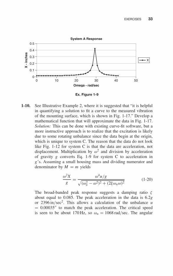
EXERCISES 33

System A Response

0

0.1

0.2

0.3

0.4

0.5

0 10 20 30 40 50

Omega - rad/sec

X -

inch

es

X

Ex. Figure 1-9

1-10. See Illustrative Example 2, where it is suggested that “it is helpfulin quantifying a solution to fit a curve to the measured vibrationof the mounting surface, which is shown in Fig. 1-17.” Develop amathematical function that will approximate the data in Fig. 1-17.Solution: This can be done with existing curve-fit software, but amore instructive approach is to realize that the excitation is likelydue to some rotating unbalance since the data begin at the origin,which is unique to system C. The reason that the data do not looklike Fig. 1-12 for system C is that the data are acceleration, notdisplacement. Multiplication by ω2 and division by accelerationof gravity g converts Eq. 1-9 for system C to acceleration ing’s. Assuming a small housing mass and dividing numerator anddenominator by M = m yields

ω2X

g= ω4u/g√

(ω2n − ω2)2 + (2ξωnω)2

(1-20)

The broad-banded peak response suggests a damping ratio ζ

about equal to 0.085. The peak acceleration in the data is 6.2gor 2396 in/sec2. This allows a calculation of the unbalance u= 0.00035′′ to match the peak acceleration. The critical speedis seen to be about 170 Hz, so ωn = 1068 rad/sec. The angular


velocity ω must be converted to hertz = ω/(2π) for the graph.With these values, Eq. 1-20 produces the graph shown here.

Amplitude G’s vs. Speed Hz

0.00

1.00

2.00

3.00

4.00

5.00

6.00

7.00

0 50 100 150 200 250 300 350

Hz

G’s

Ex. Figure 1-10

fundamentals of machine vibration and ......2 fundamentals of machine vibration and classical...

Documents