fundamentals of geobiology (knoll/fundamentals of geobiology) || supplemental images

Fundamentals of Geobiology, First Edition. Edited by Andrew H. Knoll, Donald E. Canfield and Kurt O. Konhauser.

© 2012 Blackwell Publishing Ltd. Published 2012 by Blackwell Publishing Ltd.

N2

Nitr

ifica

tion

Den

itrifi

catio

n

Organic N

Ass

imila

tion

N2O

NO

NH2OH

AmmonificationAmmoniaassimilation

Nitrogen fixation

Nitrite oxidationNitrate

reduction

Ammoniaoxidation

Anammox

NO3−

NO2−

NH4+

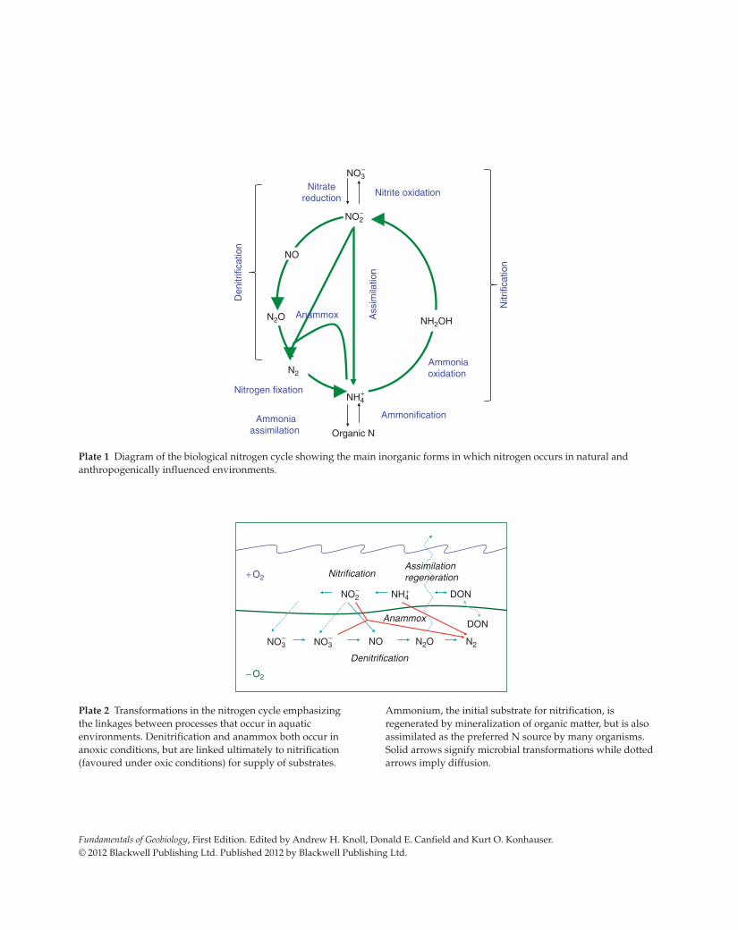
Plate 1 Diagram of the biological nitrogen cycle showing the main inorganic forms in which nitrogen occurs in natural and

anthropogenically influenced environments.

NO N2O N2

DON

+ O2

− O2

Nitrification

Denitrification

Anammox

Assimilationregeneration

DON

NO2−

NO3− NO3

−

NH4+

Plate 2 Transformations in the nitrogen cycle emphasizing

the linkages between processes that occur in aquatic

environments. Denitrification and anammox both occur in

anoxic conditions, but are linked ultimately to nitrification

(favoured under oxic conditions) for supply of substrates.

Ammonium, the initial substrate for nitrification, is

regenerated by mineralization of organic matter, but is also

assimilated as the preferred N source by many organisms.

Solid arrows signify microbial transformations while dotted

arrows imply diffusion.

Knoll_bins.indd 1Knoll_bins.indd 1 2/16/2012 2:11:57 AM2/16/2012 2:11:57 AM

–40

–20

0

20

40

60

12

4

8

0

0

0.5

1.0

1.5

0.1

1.0

10

0

2

4

6

???

Δ33S

δ33S

f -ratio

Sulfate (mM)

Sulfur reservoir

x 1020 mol

Relative BIFdeposition

Deep water

O2

H2S

Fe2+

???

???

0 500 1000 1500 2000 2500 3000 3500 4000

Time (Ma)

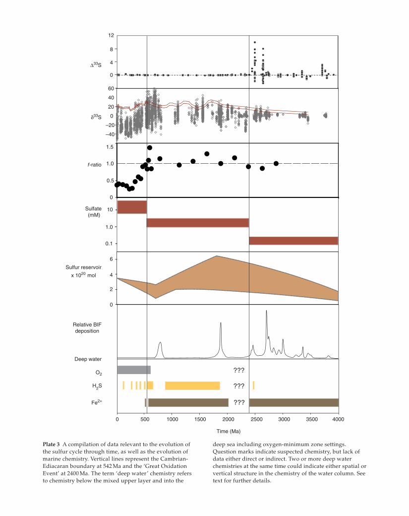
Plate 3 A compilation of data relevant to the evolution of

the sulfur cycle through time, as well as the evolution of

marine chemistry. Vertical lines represent the Cambrian-

Ediacaran boundary at 542 Ma and the ‘Great Oxidation

Event’ at 2400 Ma. The term ‘deep water’ chemistry refers

to chemistry below the mixed upper layer and into the

deep sea including oxygen-minimum zone settings.

Question marks indicate suspected chemistry, but lack of

data either direct or indirect. Two or more deep water

chemistries at the same time could indicate either spatial or

vertical structure in the chemistry of the water column. See

text for further details.


(a)HCO3

–

Ca2+ Ca2+

Ca2+

Ca2+Ca2+

S-layer

Ca2+

Anionicligands

Calcitenucleation

OH–

Cyanobacterium

CO32–

(b)+ +Fe2+ 2Fe(OH)3 Fe3O4+ 4H2O2OH–

Fe(lll)-reducing bacterium

Fe2+

2e–

Fe2+

Fe(OH)3

Magnetitenucleation

EPS

CH3COO–

Fe(OH)3

OH–

H2O + CO32– HCO3

– OH–+

HCO3– +H2O CH2O + O2 + OH–

+ +2H+ 2Fe(OH)3--> + 4OH–+ 2H2O2e– 2Fe2+

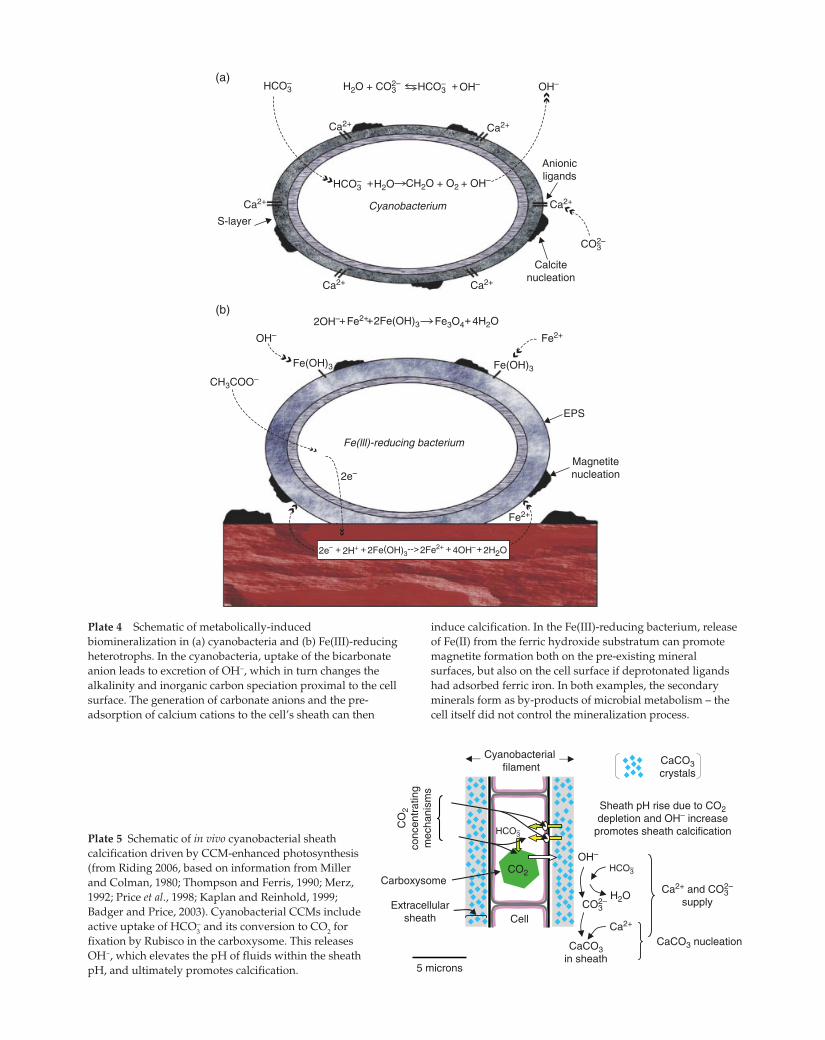
Plate 4 Schematic of metabolically-induced

biomineralization in (a) cyanobacteria and (b) Fe(III)-reducing

heterotrophs. In the cyanobacteria, uptake of the bicarbonate

anion leads to excretion of OH−, which in turn changes the

alkalinity and inorganic carbon speciation proximal to the cell

surface. The generation of carbonate anions and the pre-

adsorption of calcium cations to the cell’s sheath can then

induce calcification. In the Fe(III)-reducing bacterium, release

of Fe(II) from the ferric hydroxide substratum can promote

magnetite formation both on the pre-existing mineral

surfaces, but also on the cell surface if deprotonated ligands

had adsorbed ferric iron. In both examples, the secondary

minerals form as by-products of microbial metabolism – the

cell itself did not control the mineralization process.

HCO3–

HCO3–

Carboxysome

Extracellularsheath

Sheath pH rise due to CO2depletion and OH– increase

promotes sheath calcification

OH–

CO32–

Ca2+

H2O

CaCO3 in sheath

CO

2co

ncen

trat

ing

mec

hani

sms

Ca2+ and CO32–

supply

CaCO3 nucleation

CO2

Cyanobacterial filament

Cell

CaCO3crystals

5 microns

Plate 5 Schematic of in vivo cyanobacterial sheath

calcification driven by CCM-enhanced photosynthesis

(from Riding 2006, based on information from Miller

and Colman, 1980; Thompson and Ferris, 1990; Merz,

1992; Price et al., 1998; Kaplan and Reinhold, 1999;

Badger and Price, 2003). Cyanobacterial CCMs include

active uptake of HCO3− and its conversion to CO

2 for

fixation by Rubisco in the carboxysome. This releases

OH−, which elevates the pH of fluids within the sheath

pH, and ultimately promotes calcification.


Infe

rred

C

O2

tren

d (a

) 20

0 40

20 0

40

500

1000

0

Mill

ions

of y

ears

ago

a c

She

ath

calc

ifica

tion

in

duce

d de

spite

el

evat

ed C

O2

550–

150

Ma,

cal

cifie

d sh

eath

abu

ndan

ce b

road

ly

corr

espo

nds

with

mar

ine

carb

onat

e sa

tura

tion

stat

e

~35

0 M

a,

shea

th

calc

ifica

tion

incr

ease

as

CO

2 de

clin

ed

Saturation state Ωcalcite

Sheath calcified cyanobacteria

abundance

Cen

ozoi

c,

mar

ine

shea

th

calc

ifica

tion

scar

ce

to a

bsen

t

A

nom

alou

s el

evat

ed

satu

ratio

n st

ate

Mar

ine

wh

iting

s an

d sh

eath

ca

lcifi

catio

n re

duce

d by

lo

wer

car

bona

te

satu

ratio

n st

ate

Firs

t sh

eath

ca

lcifi

ed

cyan

obac

teria

Car

bona

te

mud

do

min

ated

sh

elve

s

Infe

rred

CC

M

indu

ctio

n as

C

O2

decl

ined

be

low

~10

PA

L

Infe

rred

in

cept

ion

of

biog

enic

‘w

hitin

gs’

She

ath

calc

ified

cy

anob

acte

ria

wid

espr

ead

GE

OC

AR

B II

I m

odel

led

CO

2 tr

end

Cal

cifie

d sh

eath

s sc

arce

b

a

Pos

sibl

y

due

to lo

w

tem

pera

ture

an

d lo

w

satu

ratio

n st

ate

10

PA

L C

O2

Infe

rred

thre

sho

ld

belo

w w

hich

C

CM

s in

duce

d

1500

Gla

ciat

ions

2 5

4 1

3 6

7 8

CO2 ratio to present-day pre-industrial atmospheric level (PAL)

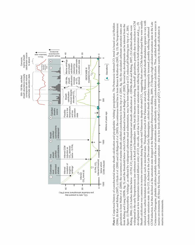
Pla

te 6

C

on

ject

ura

l h

isto

ry o

f cy

an

ob

act

eria

l m

ari

ne

shea

th c

alc

ific

ati

on

an

d p

ico

pla

nk

tic

‘wh

itin

g’

pre

cip

itati

on

. T

he

Pro

tero

zo

ic i

nfe

rred

CO

2 t

ren

d i

s b

ase

d o

n (

a)

Sh

eld

on

(2006),

(b

) K

ah

an

d R

idin

g (

2007),

(c)

Hy

de

et a

l. (2

000)

an

d (

d)

Rid

gw

ell

et a

l. (2

003);

th

e co

nti

nu

ou

s tr

end

lin

e is

fro

m B

ern

er &

Ko

thav

ala

(2001, fi

g. 13);

th

e N

eop

rote

rozo

ic

gla

ciati

on

s is

fro

m W

alt

er e

t al.

(2000);

th

e o

ccu

rren

ces

of

mari

ne

shea

th c

alc

ifie

d c

yan

ob

act

eria

is

fro

m A

rp e

t al.

(2001, fi

g. 3d

); t

he

calc

ula

ted

carb

on

ate

satu

rati

on

sta

tes

are

fro

m R

idin

g a

nd

Lia

ng

(2005b

, fi

g. 5);

an

d t

he

thre

sho

ld b

elo

w w

hic

h C

CM

s are

in

du

ced

is

base

d o

n B

ad

ger

et a

l. (2

002).

Sev

eral

key

dev

elo

pm

ents

can

be

infe

rred

fro

m t

he

fig

ure

. (1

) P

ho

tosy

nth

etic

‘w

hit

ing

s’, as

refl

ecte

d b

y w

ides

pre

ad

carb

on

ate

mu

d s

edim

enta

tio

n, m

ay

hav

e b

een

tri

gg

ered

as

CO

2 r

edu

ced

pH

bu

ffer

ing

(se

e A

rp e

t al.,

2001;

Rid

ing

, 2006).

(2)

A f

urt

her

dec

lin

e b

elo

w ~

10 P

AL

CO

2 i

nd

uce

d C

CM

dev

elo

pm

ent

an

d s

hea

th c

alc

ific

ati

on

at

~1200 M

a (

Kah

an

d R

idin

g, 2007).

(3)

Calc

ifie

d s

hea

ths

wer

e

wid

esp

read

in

th

e ea

rly

Neo

pro

tero

zo

ic (

see

refe

ren

ces

in K

no

ll a

nd

Sem

ikh

ato

v 1

998),

bu

t (4

) b

ecam

e sc

arc

e d

uri

ng

‘S

no

wb

all

’ g

laci

ati

on

s, p

oss

ibly

du

e to

red

uct

ion

in

CC

M

dev

elo

pm

ent

as

low

tem

per

atu

res

fav

ou

red

dif

fusi

ve

entr

y o

f C

O2 i

nto

cel

ls, an

d d

ue

to l

ow

er s

eaw

ate

r sa

tura

tio

n s

tate

ref

lect

ing

red

uct

ion

in

bo

th t

emp

eratu

re a

nd

pC

O2. (5

)

Sh

eath

calc

ific

ati

on

was

com

mo

n i

n m

ari

ne

env

iro

nm

ents

du

rin

g t

he

earl

y-m

id P

ala

eozo

ic d

esp

ite

elev

ate

d C

O2, su

gg

esti

ng

th

at

on

ce C

CM

s h

ad

dev

elo

ped

th

ey w

ere

read

ily

ind

uce

d w

her

e ca

rbo

n l

imit

ati

on

dev

elo

ped

, su

ch a

s m

icro

bia

l m

ats

. T

hro

ug

ho

ut

mu

ch o

f th

e P

ala

eozo

ic a

nd

earl

y M

eso

zo

ic, ca

lcif

ied

sh

eath

ab

un

dan

ce a

pp

ears

to

vary

wit

h

carb

on

ate

satu

rati

on

sta

te. (6

) A

s C

O2 d

ecli

ned

in

th

e L

ate

Dev

on

ian

-Earl

y M

issi

ssip

pia

n, ca

lcif

ied

sh

eath

ab

un

dan

ce t

emp

ora

rily

in

crea

sed

, p

oss

ibly

ref

lect

ing

en

han

ced

CC

M i

nd

uct

ion

, b

ut

then

dec

lin

ed a

s th

e sa

tura

tio

n s

tate

dro

pp

ed i

n t

he

Mis

siss

ipp

ian

-Pen

nsy

lvan

ian

(R

idin

g, 2009).

(7)

Des

pit

e a h

igh

calc

ula

ted

satu

rati

on

sta

te i

n t

he

Late

Cre

tace

ou

s-P

ala

eog

ene,

pla

nk

tic

calc

ifie

rs p

rob

ab

ly r

edu

ced

th

e act

ual

satu

rati

on

sta

te s

uff

icie

ntl

y t

o i

nh

ibit

cy

an

ob

act

eria

l ca

lcif

icati

on

. T

hu

s, c

alc

ifie

d s

hea

ths

wer

e sc

arc

e in

mari

ne

env

iro

nm

ents

. (8

) S

ince

th

e E

oce

ne,

lo

w c

arb

on

ate

satu

rati

on

– d

ue

to l

ow

lev

els

of

bo

th C

a i

on

s an

d p

CO

2– i

s re

flec

ted

in

ex

trem

e sc

arc

ity

in

sh

eath

calc

ific

ati

on

in

mari

ne

env

iro

nm

ents

.


(a) (d)

(b) (e)

(c) (f)

<121>

<110>

<121>

<110>

<121>

<110>

<121>

<110>

<121>

<110>

<121>

<110>

Lattice oxygen Fetet1Feoct2

Capping oxygen

OA

Fetet1

Feoct1

OBFetet2Feoct2Fetet1OC

Lattice oxygen

Surface A

1.2 ± 0.1 Å

3.3 ± 0.1 Å

0.4 ± 0.1 Å

Surface A’

Surface BSurface Aα β

Fetet1/Fetet2

Feoct2 Capping oxygen

4.54.03.53.02.52.0

Ver

tical

dis

tanc

e (Å

)

1.51.00.50.0

Feoct1

[111][110]

A

A’

B

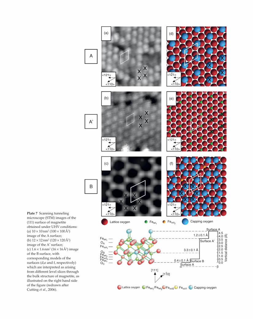
Plate 7 Scanning tunneling

microscope (STM) images of the

(111) surface of magnetite

obtained under UHV conditions:

(a) 10 × 10 nm2 (100 × 100 Å2)

image of the A surface;

(b) 12 × 12 nm2 (120 × 120 Å2)

image of the A′ surface;

(c) 1.6 × 1.6 nm2 (16 × 16 Å2) image

of the B surface, with

corresponding models of the

surfaces (d,e and f, respectively)

which are interpreted as arising

from different level slices through

the bulk structure of magnetite, as

illustrated on the right hand side

of the figure (redrawn after

Cutting et al., 2006).


4.1e + 003

12C

3.7e + 003

3.2e + 003

2.8e + 003

2.3e + 003

1.8e + 003

1.4e + 003

9.3e + 002

4.7e + 002

12.

12C14N1.0e + 003

10 um

(c)(a)

(b)

(d)

9.1e + 002

8.0e + 002

6.8e + 002

5.7e + 002

4.5e + 002

3.4e + 002

2.3e + 002

1.1e + 002

0.00

32S

4.4e + 002

3.9e + 002

3.4e + 002

2.9e + 002

2.4e + 002

1.9e + 002

1.5e + 002

97.

49.

0.00

(e)

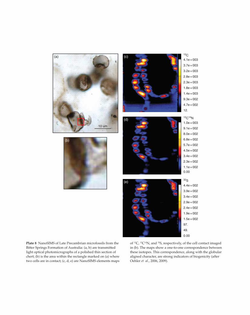
Plate 8 NanoSIMS of Late Precambrian microfossils from the

Bitter Springs Formation of Australia: (a, b) are transmitted

light optical photomicrographs of a polished thin section of

chert; (b) is the area within the rectangle marked on (a) where

two cells are in contact; (c, d, e) are NanoSIMS elements maps

of 12C, 12C14N, and 32S, respectively, of the cell contact imaged

in (b). The maps show a one-to-one correspondence between

these isotopes. This correspondence, along with the globular

aligned character, are strong indicators of biogenicity (after

Oehler et al., 2006, 2009).


Bulksolution

Carapace

Carapacesupportstructure

Basalbiofilm

Mineralsurface

Uncolonisedmineral surface

Intra-biofilmfluid flow

321.4μm

25.3μm

31.5 μm

321.4 μm

Primary colonising bacteria

Intra-biofilm bacterial colonies

Carapace bacterial colonies

Carapace polysaccharides/EPS

Basal polysaccharides/EPS

Fluid flow

Plate 9 Confocal scanning laser microscope (CSLM)

image of a biofilm grown between two quartz glass

plates by introducing a nutrient solution and inoculating

with Pseudomonas aeruginosa. Below the image is a

schematic diagram showing the various components of

the biofilm (after Brydie et al., 2004, 2009).


Fe-O4 weeks

2 weeks

1 week

Fe 2p3/2

Fe 2p1/2

× 102

5

10

15

20

25

30

35

CP

S

740 735 730 725 720 715 710 705 700Binding energy (eV)

(b)

CP

S

Fe 2p3/2

1 week

2 weeks

4 weeks

Fe 2p1/2

× 102

10

15

20

25

740 735 730 725 720 715 710 705 700Binding energy (eV)

(c) (d)

80×101

CP

S

706050403020

Fe3p

58 56 54

As 3d

2 weeks

1 weeks

4 weeks

As(V)-OAs(lll)-O

52 50 48Binding energy (eV)

46 44 42 40 38

10

(a)

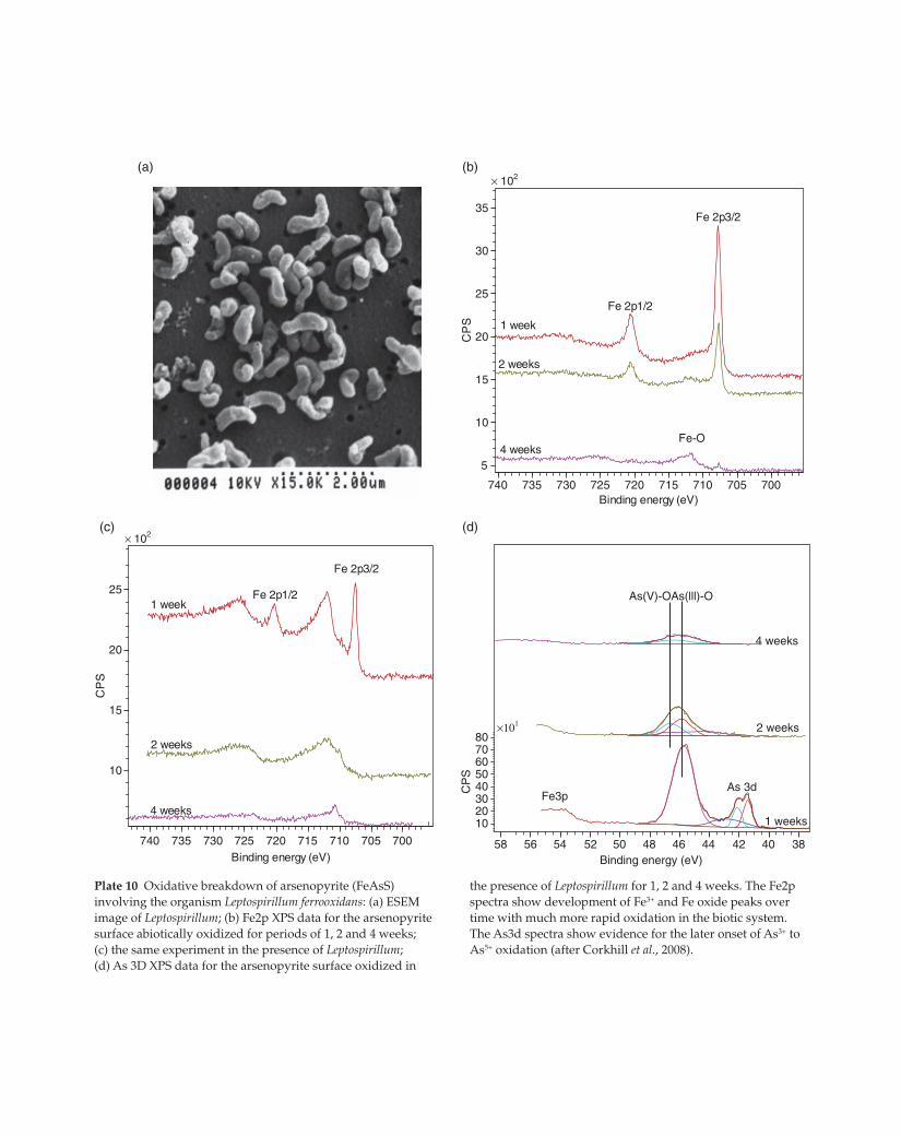
Plate 10 Oxidative breakdown of arsenopyrite (FeAsS)

involving the organism Leptospirillum ferrooxidans: (a) ESEM

image of Leptospirillum; (b) Fe2p XPS data for the arsenopyrite

surface abiotically oxidized for periods of 1, 2 and 4 weeks;

(c) the same experiment in the presence of Leptospirillum;

(d) As 3D XPS data for the arsenopyrite surface oxidized in

the presence of Leptospirillum for 1, 2 and 4 weeks. The Fe2p

spectra show development of Fe3+ and Fe oxide peaks over

time with much more rapid oxidation in the biotic system.

The As3d spectra show evidence for the later onset of As3+ to

As5+ oxidation (after Corkhill et al., 2008).


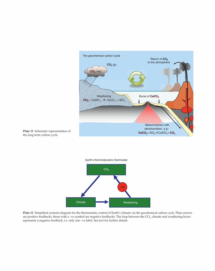
Return of CO2to the atmosphere

Burial of CaCO3WeatheringCO2 + CaSiO 3 CaCO 3 + SiO 2

Metamorphism withdecarbonation, e.g.:

The geochemical carbon cycle

CO2 (aq)

CO2 (g)

CaCO3+ SiO2 CaSiO3+ CO2Plate 11 Schematic representation of

the long-term carbon cycle.

Earth’s thermodynamic thermostat

WeatheringClimate

CO2

–ve

Plate 12 Simplified systems diagram for the thermostatic control of Earth’s climate via the geochemical carbon cycle. Plain arrows

are positive feedbacks, those with a –ve symbol are negative feedbacks. The loop between the CO2, climate and weathering boxes

represents a negative feedback, i.e. only one –ve label. See text for further details.


Linking taxonomic diversitywith metabolic activity e.g.

Raman-FISH, SIPs

Meta-genomics,transcriptomics and

proteomics

Niche characterizationEcological lifestyle

Population/community/ecosystemdynamics

Systems biologymetabolic networks

Biodiversity assessments:Who’s there?

Metabolic potential and activityassessments:

What are they doing?

Targeted enrichment

culturing

Patterns of microbial diversity

?

16S rRNA gene assessments

Statistical analyses linkingenvironmental metadatawith community structure

ABC

D GEF

JIH

13C-labeledsubstrate DNA or

RNA

Ecosystem models, testmodel predictions

Classical geneticsand biochemistry

12C13C

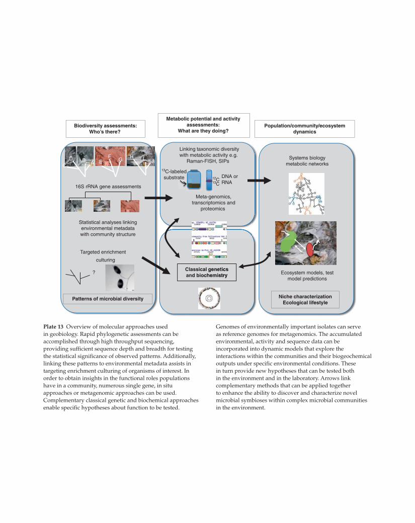
Plate 13 Overview of molecular approaches used

in geobiology. Rapid phylogenetic assessments can be

accomplished through high throughput sequencing,

providing sufficient sequence depth and breadth for testing

the statistical significance of observed patterns. Additionally,

linking these patterns to environmental metadata assists in

targeting enrichment culturing of organisms of interest. In

order to obtain insights in the functional roles populations

have in a community, numerous single gene, in situ

approaches or metagenomic approaches can be used.

Complementary classical genetic and biochemical approaches

enable specific hypotheses about function to be tested.

Genomes of environmentally important isolates can serve

as reference genomes for metagenomics. The accumulated

environmental, activity and sequence data can be

incorporated into dynamic models that explore the

interactions within the communities and their biogeochemical

outputs under specific environmental conditions. These

in turn provide new hypotheses that can be tested both

in the environment and in the laboratory. Arrows link

complementary methods that can be applied together

to enhance the ability to discover and characterize novel

microbial symbioses within complex microbial communities

in the environment.


SO42–

HS–

CH4

(a) (b)

CH2

(e–)*

(e–)*

(e–)*

(e–)*

CH3 OOH, other?

other?

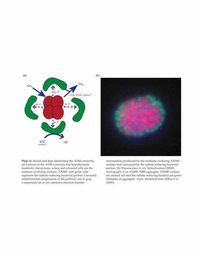
Plate 14 Model and data illustrating the AOM consortia.

(a) Cartoon of the AOM consortia and hypothesized

metabolic interactions, where red coloured cells are the

methane-oxidizing archaea ‘ANME’ and green cells

represent the sulfate-reducing bacterial partner. Currently

undetermined components of the pathway are in gray,

e-represents an as yet unknown electron transfer

intermediate produced by the methane-oxidizing ANME

archaea and consumed by the sulfate-reducing bacterial

partner. (b) Fluorescence in situ hybridization (FISH)

micrograph of an ANME/SRB aggregate. ANME archaea

are stained red and the sulfate-reducing bacteria are green.

Diameter of aggregate ∼6 μm. Modified from Dekas et al. (2009).


Tungsten electrodes

Electricsparks

5-Literflask

Condenser

10 cmBoilingwater

500-CCflask

Stopcocks forwithdrawing

samples during run

Gasmixture

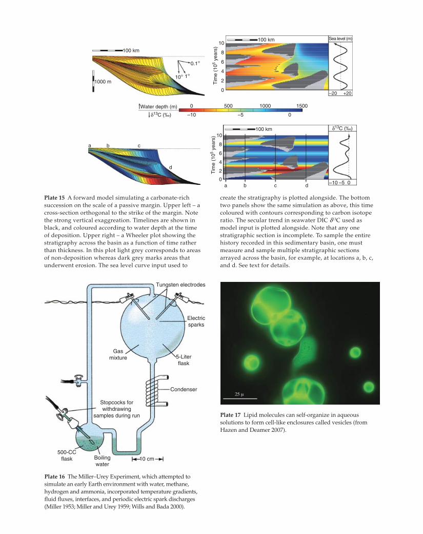
Plate 16 The Miller–Urey Experiment, which attempted to

simulate an early Earth environment with water, methane,

hydrogen and ammonia, incorporated temperature gradients,

fluid fluxes, interfaces, and periodic electric spark discharges

(Miller 1953; Miller and Urey 1959; Wills and Bada 2000).

Plate 17 Lipid molecules can self-organize in aqueous

solutions to form cell-like enclosures called vesicles (from

Hazen and Deamer 2007).

–20

Sea level (m)

+20

10100 km

8

6

4

2

0

Tim

e (1

05 ye

ars)

1000 m

100 km

10° 1°

0.1°

Water depth (m)

–10

0 500 1000 1500

0–5δ13C (‰)

a b c

d

100 km10

8

6

4

2

0a b c d –10 –5 0

Tim

e (1

05 ye

ars)

δ13C (‰)

Plate 15 A forward model simulating a carbonate-rich

succession on the scale of a passive margin. Upper left – a

cross-section orthogonal to the strike of the margin. Note

the strong vertical exaggreation. Timelines are shown in

black, and coloured according to water depth at the time

of deposition. Upper right – a Wheeler plot showing the

stratigraphy across the basin as a function of time rather

than thickness. In this plot light grey corresponds to areas

of non-deposition whereas dark grey marks areas that

underwent erosion. The sea level curve input used to

create the stratigraphy is plotted alongside. The bottom

two panels show the same simulation as above, this time

coloured with contours corresponding to carbon isotope

ratio. The secular trend in seawater DIC d13C used as

model input is plotted alongside. Note that any one

stratigraphic section is incomplete. To sample the entire

history recorded in this sedimentary basin, one must

measure and sample multiple stratigraphic sections

arrayed across the basin, for example, at locations a, b, c,

and d. See text for details.


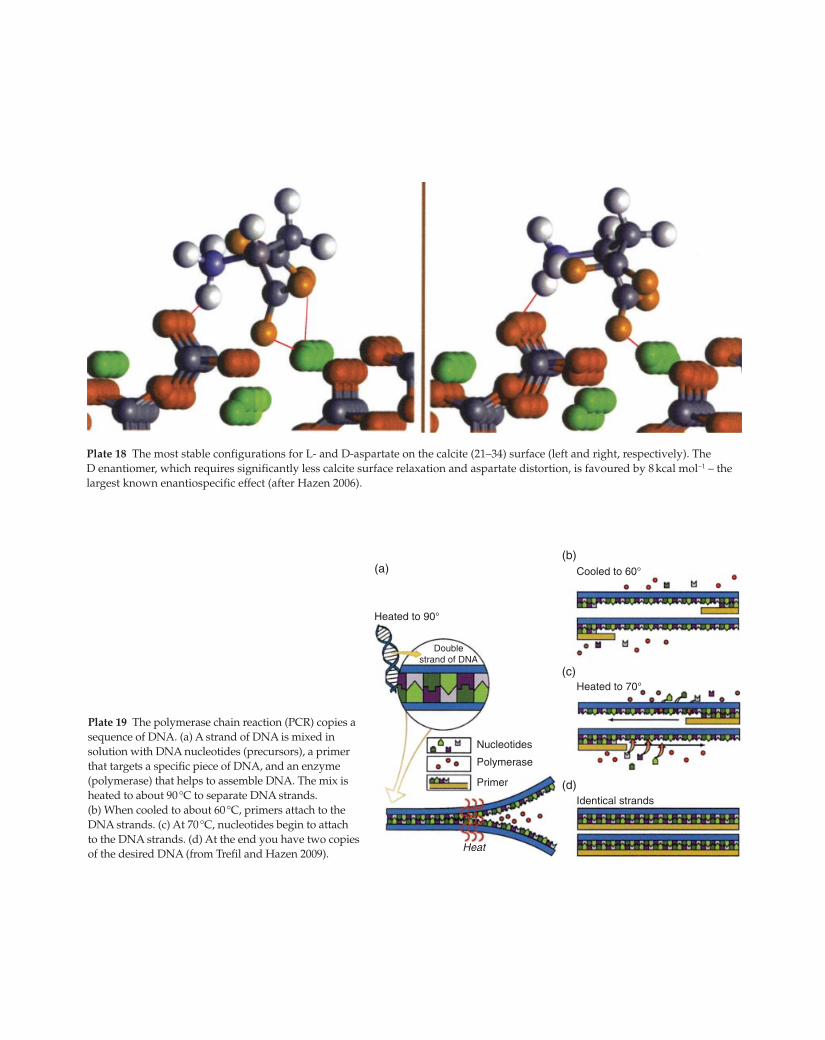
Plate 18 The most stable configurations for L- and D-aspartate on the calcite (21–34) surface (left and right, respectively). The

D enantiomer, which requires significantly less calcite surface relaxation and aspartate distortion, is favoured by 8 kcal mol−1 – the

largest known enantiospecific effect (after Hazen 2006).

(a)

(d)

(c)

(b)Cooled to 60°

Heated to 70°

Heated to 90°

Identical strands

Heat

Primer

Nucleotides

Doublestrand of DNA

Polymerase

Plate 19 The polymerase chain reaction (PCR) copies a

sequence of DNA. (a) A strand of DNA is mixed in

solution with DNA nucleotides (precursors), a primer

that targets a specific piece of DNA, and an enzyme

(polymerase) that helps to assemble DNA. The mix is

heated to about 90 °C to separate DNA strands.

(b) When cooled to about 60 °C, primers attach to the

DNA strands. (c) At 70 °C, nucleotides begin to attach

to the DNA strands. (d) At the end you have two copies

of the desired DNA (from Trefil and Hazen 2009).


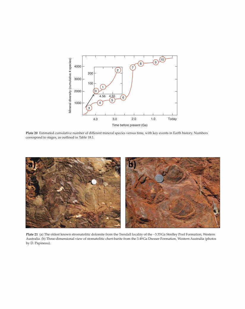
Plate 21 (a) The oldest known stromatolitic dolomite from the Trendall locality of the ∼3.35 Ga Strelley Pool Formation, Western

Australia. (b) Three-dimensional view of stomatolitic chert-barite from the 3.49 Ga Dresser Formation, Western Australia (photos

by D. Papineau).

Time before present (Ga)

4000

3000

2000

1000

Min

eral

div

ersi

ty (

cum

ulat

ive

# sp

ecie

s)

4.0 3.0 2.0

4

3

56

72

10

200

100

4.56 4.55

8 910

1.0 Today

Plate 20 Estimated cumulative number of different mineral species versus time, with key events in Earth history. Numbers

correspond to stages, as outlined in Table 18.1.


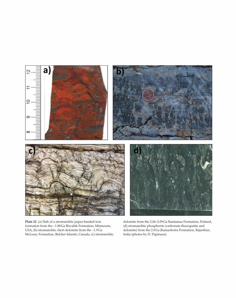
Plate 22 (a) Slab of a stromatolitic jasper banded iron

formation from the ∼1.88 Ga Biwabik Formation, Minnesota,

USA, (b) stromatolitic chert-dolomite from the ∼1.9 Ga

McLeary Formation, Belcher Islands, Canada, (c) stromatolitic

dolomite from the 2.06–2.09 Ga Rantamaa Formation, Finland,

(d) stromatolitic phosphorite (carbonate-fluorapatite and

dolomite) from the 2.0 Ga Jhamarkotra Formation, Rajasthan,

India (photos by D. Papineau).


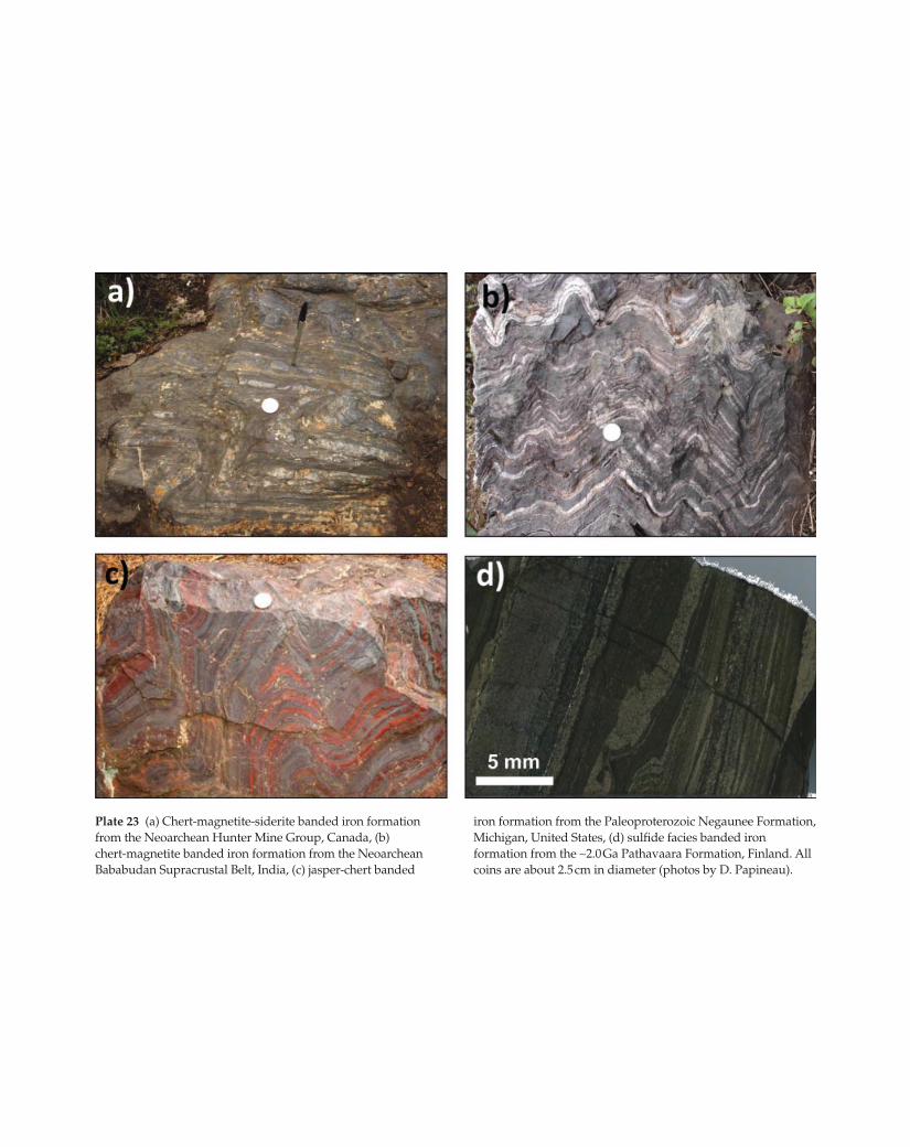
Plate 23 (a) Chert-magnetite-siderite banded iron formation

from the Neoarchean Hunter Mine Group, Canada, (b)

chert-magnetite banded iron formation from the Neoarchean

Bababudan Supracrustal Belt, India, (c) jasper-chert banded

iron formation from the Paleoproterozoic Negaunee Formation,

Michigan, United States, (d) sulfide facies banded iron

formation from the ∼2.0 Ga Pathavaara Formation, Finland. All

coins are about 2.5 cm in diameter (photos by D. Papineau).


1.50.0

0.1

0.2

0.3

0.4

2.0 2.5Age (Ga)

Hei

ght

3.0 3.5 4.0

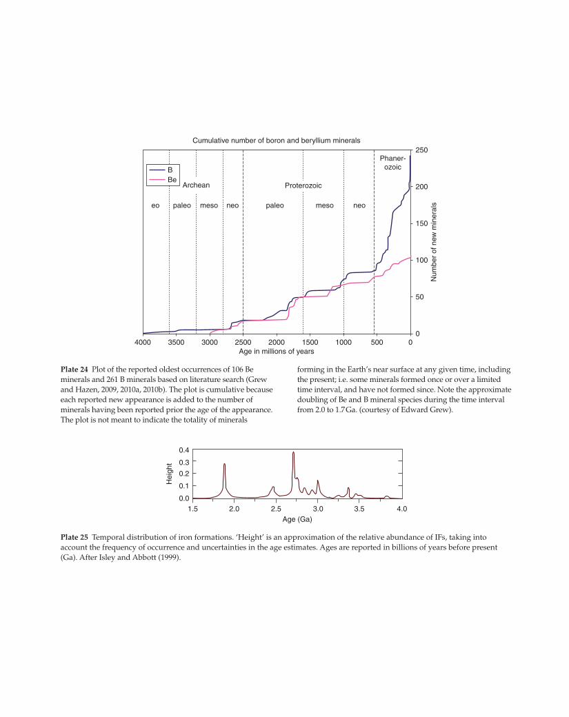
Plate 25 Temporal distribution of iron formations. ‘Height’ is an approximation of the relative abundance of IFs, taking into

account the frequency of occurrence and uncertainties in the age estimates. Ages are reported in billions of years before present

(Ga). After Isley and Abbott (1999).

BBe

Cumulative number of boron and beryllium minerals

Archean

eo paleo meso neo paleo

Proterozoic

meso neo

Phaner-ozoic

4000 3500 2500 1500 1000 500 00

50

100

150

200

250

3000 2000Age in millions of years

Num

ber

of n

ew m

iner

als

Plate 24 Plot of the reported oldest occurrences of 106 Be

minerals and 261 B minerals based on literature search (Grew

and Hazen, 2009, 2010a, 2010b). The plot is cumulative because

each reported new appearance is added to the number of

minerals having been reported prior the age of the appearance.

The plot is not meant to indicate the totality of minerals

forming in the Earth’s near surface at any given time, including

the present; i.e. some minerals formed once or over a limited

time interval, and have not formed since. Note the approximate

doubling of Be and B mineral species during the time interval

from 2.0 to 1.7 Ga. (courtesy of Edward Grew).


250020001500

Neo NeoMeso Meso

Archean

Paleo Paleo

Age (Ma)

10005000

–4

0

4

8

12

Phanerozoic Proterozoic

3000 3500

δ13C

(‰

, PD

B)

G.O

.E

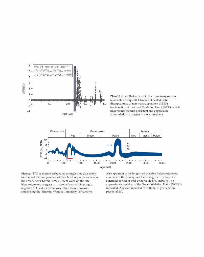
Plate 27 δ 13C of marine carbonates through time as a proxy

for the isotopic composition of dissolved inorganic carbon in

the ocean. After Karhu (1999). Recent work on the late

Neoproterozoic suggests an extended period of strongly

negative δ 13C values (even lower than those shown) –

comprising the ‘Shuram–Wonoka‘. anomaly (left arrow).

Also apparent is the long-lived positive Paleoproterozoic

anomaly of the Lomagundi Event (right arrow) and the

extended period of mid-Proterozoic δ13C stability. The

approximate position of the Great Oxidation Event (GOE) is

indicated. Ages are reported in millions of years before

present (Ma).

G.O

.E.

4

2

0

Δ33S

(‰)

–2

–4

0 1.0

Δ33S = δ33S – 1000∗((1 + δ34S / 1000)0.515– 1)

δ34S = ((34S / 32S)samp/ (34S / 32S)r e f– 1)∗1000

δ33S = ((33S / 32S)samp/ (33S / 32S)re f– 1)∗1000

2.0

Age (Ga)

3.0 4.0

6

8

10

12

Plate 26 Compilation of Δ33S data from many sources

(available on request). Clearly delineated is the

disappearance of non-mass-dependent (NMD)

fractionation at the Great Oxidation Event (GOE), which

fingerprints the first persistent and appreciable

accumulation of oxygen in the atmosphere.


–1

–2

–3

–4

–5

–6

–7

0

1.9 2.0 2.1 2.2 2.3 2.4 2.5

0.0 1.0 2.0 3.0 4.0

Age (Ga)

Metazoans

1001–10

<<10–3

“G.O.E”~2.4

log

pO

2 (a

tm)

[O2 ]atm (%

PA

L)

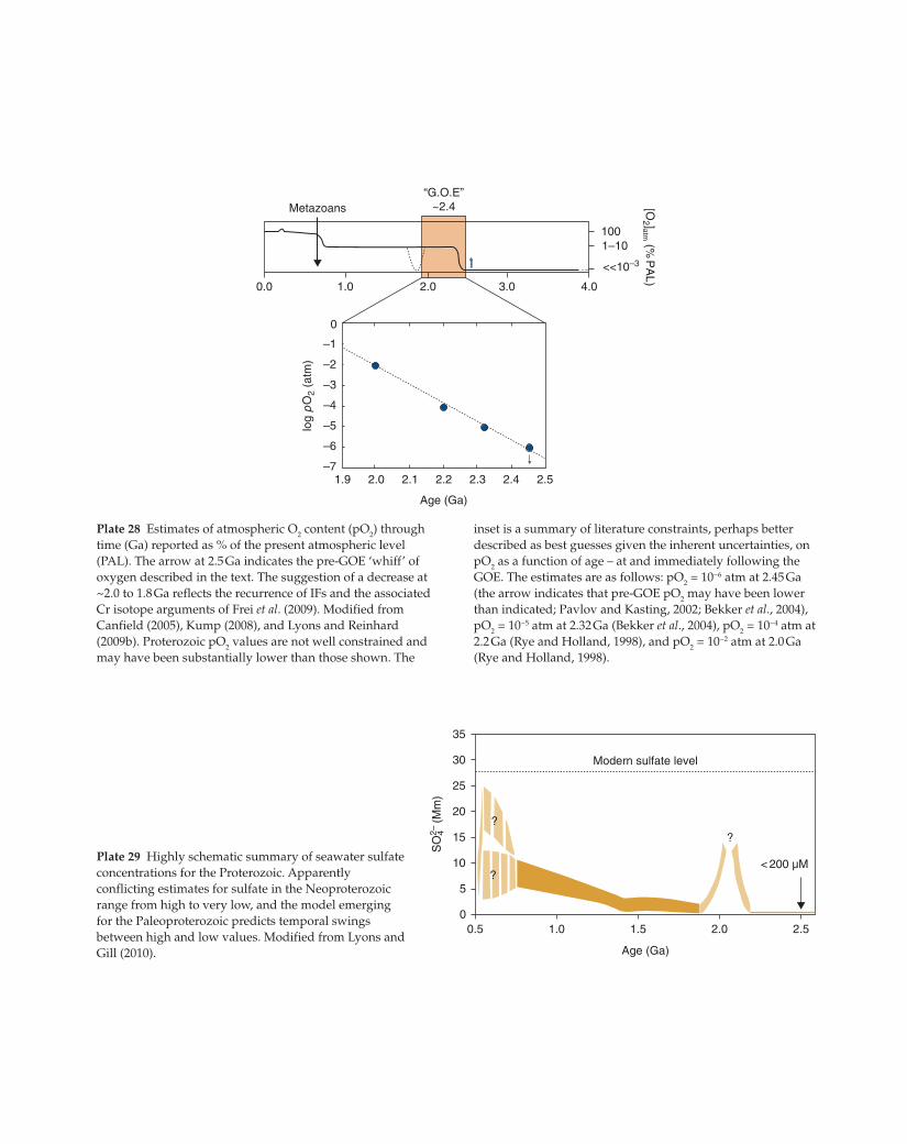
Plate 28 Estimates of atmospheric O2 content (pO

2) through

time (Ga) reported as % of the present atmospheric level

(PAL). The arrow at 2.5 Ga indicates the pre-GOE ‘whiff’ of

oxygen described in the text. The suggestion of a decrease at

~2.0 to 1.8 Ga reflects the recurrence of IFs and the associated

Cr isotope arguments of Frei et al. (2009). Modified from

Canfield (2005), Kump (2008), and Lyons and Reinhard

(2009b). Proterozoic pO2 values are not well constrained and

may have been substantially lower than those shown. The

inset is a summary of literature constraints, perhaps better

described as best guesses given the inherent uncertainties, on

pO2 as a function of age – at and immediately following the

GOE. The estimates are as follows: pO2 = 10−6 atm at 2.45 Ga

(the arrow indicates that pre-GOE pO2 may have been lower

than indicated; Pavlov and Kasting, 2002; Bekker et al., 2004),

pO2 = 10−5 atm at 2.32 Ga (Bekker et al., 2004), pO

2 = 10−4 atm at

2.2 Ga (Rye and Holland, 1998), and pO2 = 10−2 atm at 2.0 Ga

(Rye and Holland, 1998).

SO

42–(M

m)

35

30

25

20

15

10

5

00.5 1.0 1.5 2.0 2.5

Age (Ga)

< 200 μM

?

Modern sulfate level

?

?

Plate 29 Highly schematic summary of seawater sulfate

concentrations for the Proterozoic. Apparently

conflicting estimates for sulfate in the Neoproterozoic

range from high to very low, and the model emerging

for the Paleoproterozoic predicts temporal swings

between high and low values. Modified from Lyons and

Gill (2010).


60

40

20

0

–20

–40

–600

δ34S

(‰

VC

DT

)

0.5 1.0 1.5 2.0

Age (Ga)

2.5 3.0 3.5 4.0

80

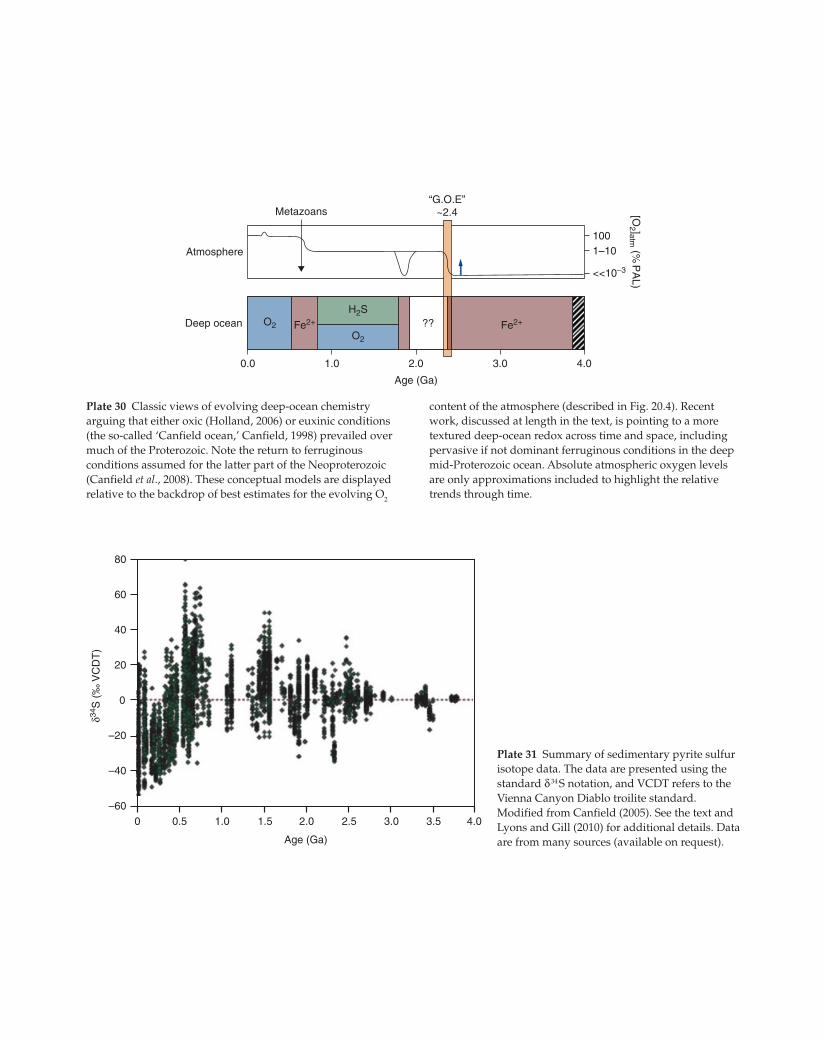
Plate 31 Summary of sedimentary pyrite sulfur

isotope data. The data are presented using the

standard δ 34 S notation, and VCDT refers to the

Vienna Canyon Diablo troilite standard.

Modified from Canfield (2005). See the text and

Lyons and Gill (2010) for additional details. Data

are from many sources (available on request).

O2O2

Fe2+ Fe2+

H2S

0.0 1.0 2.0 3.0 4.0

Age (Ga)

Atmosphere

Deep ocean

Metazoans“G.O.E”

~2.4

1001–10

<<10–3

[O2 ]atm

(%P

AL)

??

Plate 30 Classic views of evolving deep-ocean chemistry

arguing that either oxic (Holland, 2006) or euxinic conditions

(the so-called ‘Canfield ocean,’ Canfield, 1998) prevailed over

much of the Proterozoic. Note the return to ferruginous

conditions assumed for the latter part of the Neoproterozoic

(Canfield et al., 2008). These conceptual models are displayed

relative to the backdrop of best estimates for the evolving O2

content of the atmosphere (described in Fig. 20.4). Recent

work, discussed at length in the text, is pointing to a more

textured deep-ocean redox across time and space, including

pervasive if not dominant ferruginous conditions in the deep

mid-Proterozoic ocean. Absolute atmospheric oxygen levels

are only approximations included to highlight the relative

trends through time.


δ13C (‰)

Pristane & phytane

Pristane & phytane

ca. 550 Myr

n-alkanesn-alkanes

Kerogen

Kerogen–26

–29

–32

“Precambrian” “Phanerozoic”

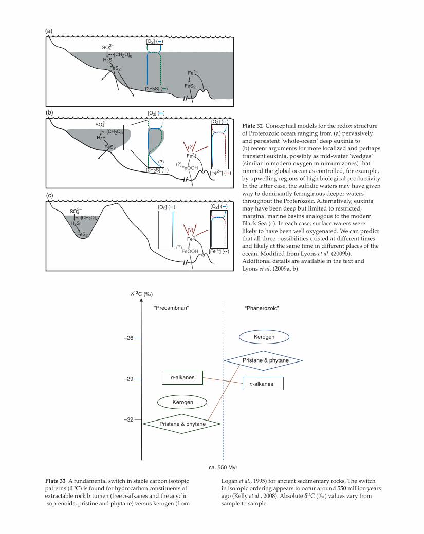
Plate 33 A fundamental switch in stable carbon isotopic

patterns (δ13C) is found for hydrocarbon constituents of

extractable rock bitumen (free n-alkanes and the acyclic

isoprenoids, pristine and phytane) versus kerogen (from

Logan et al., 1995) for ancient sedimentary rocks. The switch

in isotopic ordering appears to occur around 550 million years

ago (Kelly et al., 2008). Absolute δ13C (‰) values vary from

sample to sample.

(a)

(b)

(c)

[O2] ( )

[ΣH2S] ( )

[CH2O]xH2S

FeS2

SO42–

Fe2+

FeS2

[ΣH2S] ( )

(?)Fe2+

[CH2O]xH2S

FeS2

FeOOH(?)

[O2] ( )

[O2] ( )SO4

2–

(?)

[Fe2+] ( )

[O2] ( ) [O2] ( )SO4

2–

FeOOH(?)

(?)

[Fe ] ( )

Fe2+

[CH2O]xH2S

FeS2

Plate 32 Conceptual models for the redox structure

of Proterozoic ocean ranging from (a) pervasively

and persistent ‘whole-ocean’ deep euxinia to

(b) recent arguments for more localized and perhaps

transient euxinia, possibly as mid-water ‘wedges’

(similar to modern oxygen minimum zones) that

rimmed the global ocean as controlled, for example,

by upwelling regions of high biological productivity.

In the latter case, the sulfidic waters may have given

way to dominantly ferruginous deeper waters

throughout the Proterozoic. Alternatively, euxinia

may have been deep but limited to restricted,

marginal marine basins analogous to the modern

Black Sea (c). In each case, surface waters were

likely to have been well oxygenated. We can predict

that all three possibilities existed at different times

and likely at the same time in different places of the

ocean. Modified from Lyons et al. (2009b).

Additional details are available in the text and

Lyons et al. (2009a, b).


Opi

stho

kont

sAm

oebo

zoan

s

Red algae

Green algae

& land plantsH

apto

phyt

esDiat

oms

Brown algae

Chromalveolates

Plants

Rhizarians

Excavates

Choanoflagellates

Animals

Fungi

Lobose amoebae

Slime m

olds

Cili

ates

Api

com

plex

ans

Din

ofla

gella

tes

Oom

ycet

es

Chrysophyte

s

Foraminifers

RadiolariansCercozoansEuglenidsKinetoplastids

Parabasalids

Diplom

onads

Xanthophyte

algae

Uni

kont

s

Bikonts

1200 Ma

750 Ma

750

Ma

750 Ma

1000 Ma

Tappania850 Mafungus?

Melanocyrillium~750 Ma

lobose amoebae

Melicerion~750 Ma

cercozoan

Palaeovaucheria>1000 Ma

xanthophyteBangiomorpha~1200 Mared alga

Protocladus~750 Ma

green alga

Chlorarachniophytes

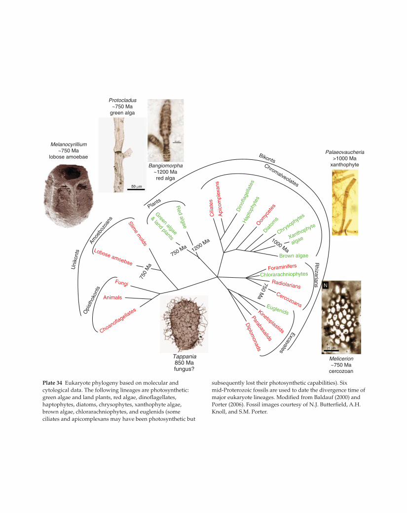
Plate 34 Eukaryote phylogeny based on molecular and

cytological data. The following lineages are photosynthetic:

green algae and land plants, red algae, dinoflagellates,

haptophytes, diatoms, chrysophytes, xanthophyte algae,

brown algae, chlorarachniophytes, and euglenids (some

ciliates and apicomplexans may have been photosynthetic but

subsequently lost their photosynthetic capabilities). Six

mid-Proterozoic fossils are used to date the divergence time of

major eukaryote lineages. Modified from Baldauf (2000) and

Porter (2006). Fossil images courtesy of N.J. Butterfield, A.H.

Knoll, and S.M. Porter.


Kimberella

540

545

550

555

560

565

570

575

580

585

590

595

600

605

610

615

620

625

630

635

640

Edi

acar

anC

ambr

ian

Cry

ogen

ian

–8 –4 0 4

δ13C (‰)

Marinoan (Nantuo) Glaciation

Gaskiers Glaciation

EN3 (Shuram)

EN1

EN2

Sou

th C

hina

DP

A

Aus

tral

ian

DP

A

Dou

shan

tuo

anim

al e

mbr

yos,

cni

daria

ns(?

)

Larg

e st

em-g

roup

ani

mal

s(?)

Larg

e m

obile

bila

teria

ns

Ani

mal

bio

min

eral

izat

ion

Dou

shan

tuo

mac

roal

gae

Fractofusus

Kimberella

Cloudina

Konglingiphyton

Megaclonophycus

Tianzhushania

Meghystricho-sphaeridium

Tanarium

Sinocyclocyclicus

?? ??

????

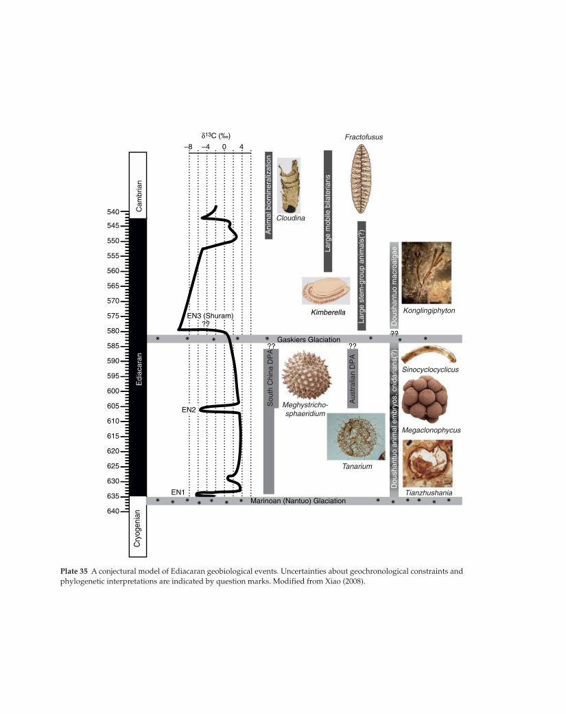
Plate 35 A conjectural model of Ediacaran geobiological events. Uncertainties about geochronological constraints and

phylogenetic interpretations are indicated by question marks. Modified from Xiao (2008).


Age (Myr)

Neogene

Penn.

Miss.

Silu

r.P

aleo

c.C

reta

ceou

sJu

rass

icT

riass

icP

erm

ian

Dev

onia

nO

rdov

icia

nC

ambr

ian

Paleoc.

Eoc.

Early

Oligoc.

Late

Early

Late

Early

Middle

Late

Early

Late

Middle

Late

Early

MiddleLate

Early

Middle

Middle

Late

EarlyMiddle

Early

Middle

Late

50

100

150

200

250

300

350

400

450

500

F

J

K

M

R

O

B

A

G

C

H

I

L

P

D

N

Q

(o)?

Ordovician

Silurian

0 1 2 3 64 5 0–2 –1–3–4–5

Sedgwickiizone

Convolutuszone

–27–28–29–30–31

(n)

(m)

Llandov.

Wenl.

0 1 2 3 64 5–1 –2 –1–3–4–5–6

(l)Ludlow

Wenlock

–2–3–4–5–60 1 2 3 64 5 7

(d)

E. Trias.

M. Trias.

0 1 2 3 4–1 7 8

zoneYabeina

Neoschw.zone

EarlyGuad.

5 6 73 4

(f)

(h)

Serp.

Tournais.

Visean

21 222019 230 1 2 3 64 5

(p)

Mohawk

Chazyan

0 1 2 3 4–2 –1–3

Marj.

Delam.

E. Cam.

0 1 2–2 –1–3 –4–5–6–7–8–9–10–11

(r)Marj.

Sunwapt.

Stept.

0 1 2 3 4–2 –1–3 5

(q)δ13C

δ13C

δ13C

δ13C

δ13C

δ13C

δ13C

δ13C δ13C

δ13C

δ13C

δ13C

δ13C

δ13C

δ13C

δ13C

δ13C

δ13C

0 1 2 3 4–2 –1–3 –4–5–6–7–8–9–10

Silur.

Devon.(k)

(j)Givet.

Frasn.

Famenn.

–3–4–5–60 1 2 3

(i)

Mississippian

1 2 3 64 5 7 –2 –1–3–4–5–6–7–8 0

Famennian

E

Guad.

Loping.

0 1 2 3 4 5–2 –1–3 –3–4–5–6–7

(g)

(a)

34Ma

Eoc.

Olig.

0 1 2 0 1 2

33Ma

(b)

Paleoc.

Eoc.

0 1 2–1

57.2Ma

57.4Ma

0–2 –1

Perm.

Trias.

–2 –1–3–4–5–6–70 1 2 3 4–2 –1

(e)

–6–7–8–9–10

Stept.

Marj.

δ18O

δ18O

δ18O

δ18O

δ18O

δ18O

δ18O

δ18O

δ18O

δ18O

δ18O

δ18O δ18O

δ18O

(c)

Trias.

Jur.

0 1 2–2 –11 2 3 4 5

Plate 36 Stable isotope excursions that have been documented

in shallow marine strata in association with mass extinctions.

Eighteen intervals (A–R) contain a total of 26 such δ13 C

excursions. Corresponding to these, and trending in the same

direction, are 19 published δ18 O excursions, which are

displayed in the plots to the right of those depicting δ13 C.

Encircled letters on the left indicate temporal positions of

excursions. Blue indicates association with global cooling and

red, with global warming; black indicates absence of published

evidence of associated climate change. Horizontal scales

represent magnitudes of δ13 C and δ18 O excursions in ‰. Light

δ13 C in N is for organic carbon rather than carbonates, and

heavy δ18 O in H is for conodonts rather than bulk or skeletal

carbonate. Ordinates represent stratigraphic positions of

samples and are neither precisely linear with respect to time

nor scaled the same for all graphs (after Stanley, 2010).


fundamentals of geobiology (knoll/fundamentals of geobiology) || supplemental images

Documents