fundamental cad algorithms - computer-aided design of...
TRANSCRIPT
IEEE TRANSACTIONS ON COMPUTER AIDED DESIGN OF INTEGRATED CIRCUITS AND SYSTEMS, VOL. 19, NO. 12, DECEMBER 2000 1449
Fundamental CAD AlgorithmsMelvin A. Breuer, Fellow, IEEE, Majid Sarrafzadeh, Fellow, IEEE, and Fabio Somenzi
Abstract—Computer-aided design (CAD) tools are now makingit possible to automate many aspects of the design process. This hasmainly been made possible by the use of effective and efficient algo-rithms and corresponding software structures. The very large scaleintegration (VLSI) design process is extremely complex, and evenafter breaking the entire process into several conceptually easiersteps, it has been shown that each step is still computationally hard.To researchers, the goal of understanding the fundamental struc-ture of the problem is often as important as producing a solutionof immediate applicability. Despite this emphasis, it turns out thatresults that might first appear to be only of theoretical value aresometimes of profound relevance to practical problems.
VLSI CAD is a dynamic area where problem definitions arecontinually changing due to complexity, technology and designmethodology. In this paper, we focus on several of the fundamentalCAD abstractions, models, concepts and algorithms that have hada significant impact on this field. This material should be of greatvalue to researchers interested in entering these areas of research,since it will allow them to quickly focus on much of the keymaterial in our field. We emphasize algorithms in the area of test,physical design, logic synthesis, and formal verification. Thesealgorithms are responsible for the effectiveness and efficiency of avariety of CAD tools. Furthermore, a number of these algorithmshave found applications in many other domains.
Index Terms—Algorithms, computer-aided design, computa-tional complexity, formal verification, logic synthesis, physicaldesign, test.
I. INTRODUCTION
T HE TECHNOLOGICAL revolution represented by verylarge scale integration (VLSI) has opened new horizons in
digital design methodology. The size and complexity of VLSIsystems demands the elimination of repetitive manual opera-tions and computations. This motivates the development of au-tomatic design systems. To accomplish this task, fundamentalunderstanding of the design problem and full knowledge of thedesign process are essential. Only then could one hope to effi-ciently and automatically fill the gap between system specifica-tion and manufacturing. Automation of a given design processrequires its algorithmic analysis. The availability of fast andeasily implementable algorithms is essential to the discipline.
Because of the inherent complexity of the VLSI designproblem, it is partitioned into simpler subproblems, the anal-ysis of each of which provides new insights into the original
Manuscript received January 31, 2000. This paper was recommended by As-sociate Editor M. Pedram.
M. A. Breuer is with the Department of Electrical Engineering - Systems,University of Southern California, Los Angeles, CA 90089 USA (e-mail:[email protected]).
M. Sarrafzadeh is with the Computer Science Department, the University ofCalifornia, Los Angeles, CA 90095 USA (e-mail: [email protected]).
F. Somenzi is with the Department of Electrical and Computer Engineering,University of Colorado, Boulder, CO 80302 USA (e-mail: [email protected]).
Publisher Item Identifier S 0278-0070(00)10450-6.
problem as a whole. In this framework, the objective is to viewthe VLSI design problem as a collection of subproblems; eachsubproblem should be efficiently solved and the solutions mustbe effectively combined.
Given a problem, we are to find efficient solution methods.A data structure is a way of organizing information; sometimesthe design of an appropriate data structure can be the foundationfor an efficient algorithm. In addition to the design of new datastructures, we are interested in the design of efficient solutionsfor complex problems. Often such problems can be representedin terms of trees, graphs, or strings.
Once a solution method has been proposed, we seek to find arigorous statement about its efficiency; analysis of algorithmscan go hand-in-hand with their design, or can be applied toknown algorithms. Some of this work is motivated in part bythe theory of NP-completeness, which strongly suggests thatcertain problems are just too hard to always solve exactly andefficiently. Also, it may be that the difficult cases are relativelyrare, so we attempt to investigate the behavior of problems andalgorithms under assumptions about the distribution of inputs.Probability can provide a powerful tool even when we do not as-sume a probability distribution of inputs. In an approach calledrandomization, one can introduce randomness into an algorithmso that even on a worst case input it works well with high prob-ability.
Most problems that arise in VLSI CAD are NP-complete orharder; they require fast heuristic algorithms, and benefit fromerror bounds. Robustness is very important—the program mustwork well even for degenerate or somewhat malformed input.Worst case time complexity is important, but the program shouldalso be asymptotically good in the average case, since invariablypeople will run programs on much larger inputs than the devel-opers were anticipating. It is also important that the programrun well on small inputs. Any algorithms used must be simpleenough so that they can be implemented quickly and changedlater if necessary.
In this paper, we describe fundamental algorithms that havebeen proposed in the area of test, physical design, logic syn-thesis, and formal verification. This paper is organized as fol-lows. In Section II, we review fundamental algorithms in thearea of test. Then, in Section III, we address physical designproblems and review various techniques. In Section IV, we studylogic synthesis and formal verification. Finally, we conclude inSection V.
II. FUNDAMENTAL ALGORITHMS IN TEST
A. Introduction
In this section, we focus on several issues related to post-man-ufacturing testing of digital chips. One comprehensive test oc-curs after packaging, and often involves the use of automatic
0278–0070/00$10.00 © 2000 IEEE
Authorized licensed use limited to: UNIVERSITY OF WINDSOR. Downloaded on May 19, 2009 at 18:19 from IEEE Xplore. Restrictions apply.
1450 IEEE TRANSACTIONS ON COMPUTER AIDED DESIGN OF INTEGRATED CIRCUITS AND SYSTEMS, VOL. 19, NO. 12, DECEMBER 2000
test equipment (ATE). Another involves testing of chips in thefield. A major part of these tests are carried out using nonfunc-tional data, at less than functional clock rates, and where onlystatic (logic level) voltages are measured. This aspect of the testproblem has been highly automated and is the focus of our at-tention. The major subareas of test that lie within the scope ofCAD include test generation for single stuck-at-faults (SSFs),diagnosis, fault simulation, design-for-test (DFT) and built-inself-test (BIST). The latter two topics deal primarily with testsynthesis and will not be dealt with in this paper. For a generaloverview of this topic, the reader is referred to [1].
Initially, we restrict our attention to combinational logic. Atestfor a stuck-at fault in a combinational logic circuit C con-sists of an input test pattern that 1) produces an error at the siteof the fault and 2) propagates the error to a primary output.Au-tomatic test pattern generation(ATPG) deals with developingan algorithm for constructing a test patternthat detects a fault
. Diagnosisdeals, in part, with 1) generating tests that differ-entiate between a subset of faults and 2) given the results ofapplying a test and observing its response, determining whatfaults can or cannot exists in C.Fault simulationdeals with de-termining which faults out of a class of faults are detected by atest sequence. In addition, the actual output sequence of a faultycircuit can be determined.
To automatically generate fault detection and diagnostic testsfor a sequential circuit is quite complex, and for most large cir-cuits is computationally infeasible. Thus, designers have devel-opeddesign-for-testtechniques, such as scan design, to simplifytest generation. Going a step further, test engineers have devel-oped structures that can be embedded in a circuit that either to-tally or to a large extent eliminate the need for ATPG. Thesestructuresgeneratetests in real or near real time within the cir-cuit itself, andcompact(compress) responses into a finalsig-nature. Based upon the signature one can determine whether ornot the circuit is faulty, and in some cases can actually diagnosethe fault. This area is referred to asbuilt-in self-test.
Two key concepts associated with test generation arecontrol-lability andobservability. For example, to generate a test for aline A that is stuck-at-1, it is necessary that the circuit be set intoa state, or controlled, so that in the fault free circuit 0. Thiscreates an error on line A. Next it is necessary that this error bepropagated to an observable signal line such as an output. Scandesign makes test generation much easier since flip-flops can beeasily made to be pseudoobservable and controllable.
There are five key components associated with most test al-gorithms or related software systems; namely, 1) a fault model,2) a fault pruning process, 3) a value system and data structure,and 4) the test procedure itself. The test procedure may deal withtest generation, fault simulation or diagnosis.
Manufacturing tests deal with the problem of identifying de-fective parts, e.g., a defective chip. Defects, such as extra metalor thin gate oxide are oftenmodeledusing functional concepts,such as a line stuck-at one or zero, two lines shorted together,or a gate or path whose delay is unacceptably high. In gen-eral, the number of faults associated with many models is ex-tremely high. For example, if there aresignal lines in a cir-cuit, the number of multiple stuck-at faults is bounded by.In many cases, researchers have developed quite sophisticated
techniques for reducing the number of faults that need be ex-plicitly considered by a test system. These techniques fall intothe general category offault pruning, and include the conceptsof fault dominance and equivalence.
Very often the efficiency of a test system is highly dependenton the data structures and value system employed. In test gen-eration, acompositelogic system is often used so one can keeptrack of the logic value of a line in both a fault-free and faultycircuit.
Finally, the test algorithm itself must deal with complex is-sues and tradeoffs related to time complexity, accuracy and faultcoverage.
To give the reader a flavor of some of the key results in thisfield, we focus on the following contributions: 1) the D-algo-rithm test generation methodology for SSFs, 2) concurrent faultsimulation, and 3) effect-cause fault diagnosis.
B. Test Generation for Single Stuck-At Faults in CombinationalLogic
The D-Algorithm: The problem of generating a test patternfor a SSF in a combinational logic circuit is an NP-hard
problem, and is probably the most famous problem in testing. In1960, J. Paul Roth published his now famous D-algorithm [2],which has remained one of the center pieces of our field. Thiswork employed many important contributions including the useof the cubical complex notation, backtrack programming to ef-ficiently handle implicit enumeration, and the unique conceptsof D-cubes, error propagation (D-drive) and line justification.
The D-algorithm employs a five-valued composite logicsystem where , , , and
. Here, implies that is the value of a line inthe fault free circuit, and is its value in the faulty circuit.represents an unspecified logic value. Initially all lines in acircuit are set to . A represents an error in a circuit.To create an initial error one sets a line that is– –0 to a 1,represented by a , or if – –1 to a 0, represented by a.
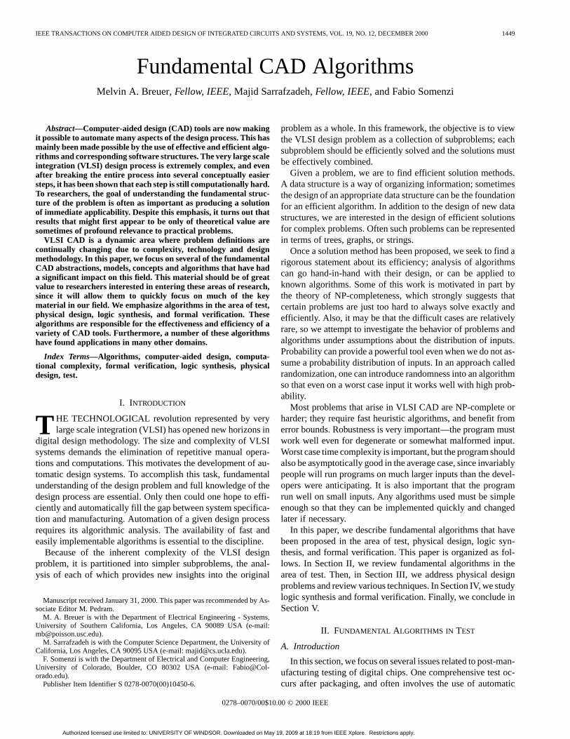
A form of forward and backward simulation is carried outby a process known asimplication , where a line at value ischanged to one of the other line values. Fig. 1(b) shows the truthtable for aNAND gate. It is easy to extend this table to includecomposite line values. So if and , then forwardimplication would set . Fig. 1(c) illustrates some examplesof backward implication. and are implied forward andbackward in the same manner based on the truth table shownin Fig. 1(d). Note that for any cube, such asall “ ” entries can be complement to form another logicallycorrect cube, such as .
The D-algorithm employs the concept ofJ-frontier andD-frontier to keep track of computations to be done as well aslead to an orderly backtrack mechanism. TheJ-frontier is a listthat contains the name of each gate whose output is assigneda logic value that is not implied by the input values to thegate, and for which no unique backward implications exists.For example if and , then there are twoways (choices) for satisfying this assignment, namely or
. These gates are candidates forline justification.
Authorized licensed use limited to: UNIVERSITY OF WINDSOR. Downloaded on May 19, 2009 at 18:19 from IEEE Xplore. Restrictions apply.
BREUERet al.: FUNDAMENTAL CAD ALGORITHMS 1451
Fig. 1. Logic system.
TheD-frontier is a list of all gates whose outputs areandwhich have one or more or input values. These gates arecandidates forD-drive.
A procedureimply-and-checkis executed whenever a line isset to a new value. This procedure carries out all forward andbackward (unique) implications based on the topology and gatesin a circuit. The version ofimply-and-checkpresented here isan extention of the original concepts and makes the proceduresomewhat more efficient.
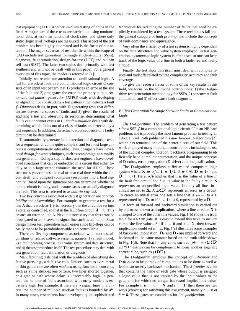
Example 1: As an example, consider the circuit shown inFig. 2(a). Since all gates have a single output we use the samesymbol to identify both a gate and its output signal. Also, wedenote line – –1(0) by .
Consider the fault . We can consider a pseudoelementplaced on this line whose input isand output is . We use thenotation to denote a line value assigned in stepof thealgorithm. We also use the symbols, to denote forwardand backward implication, respectively, andto denote justifi-cation. Since , then . TheD-frontier
, andJ-frontier .
To drive a or to a primary output, we can select anelement from theD-frontier and carryout a process known asD-drive. If we select gate , then by assigning weget , and implications results in and
. Now D-frontier and theJ-frontier is stillempty. If we next drive the error through gate to theprimary output, we require . Again, carryingout imply-and-checkwe get and which inturn implies . But since has already been assignedthe value a conflict exists. Conflicts are dealt with by back-tracking to the last step where a choice exists and selecting a dif-ferent choice. Naturally, this must be done in an orderly way sothat all possible assignments are implicitly covered. In our case,we undo all assignments associated with step 2 and selectrather than from theD-frontier. This results in andeventually with and a test .
This example illustrates the need formultiple-path sensitiza-tion. Note that the test also detects additional faults such as,
and . Later, we see that fault simulation is an efficient wayof determining all the SSFs detected by a test pattern.
Fig. 2. Circuit for Example 1.
Example 2: To illustrate the concept of line justification con-sider the fault . Here, we have and asshown in Fig. 2(c). After weD-drive through gate we have
andJ-frontier . Assume we choseto remove from theJ-frontier to be processed first. Then oneway to justify is to set , which results in severalimplications. We continue solving justification problems untilJ-frontier . If a conflict occurs, backtracking is carriedout.
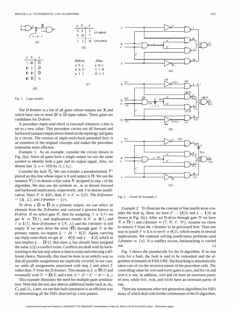
Fig. 3 shows the pseudocode for the D-algorithm. If no testexist for a fault, the fault is said to beredundantand the al-gorithm terminates in FAILURE. Backtracking is automaticallytaken care of via the recursive nature of the procedure calls. Thecontrolling value forAND andNAND gates is zero, and forORandNOR it is one. In addition,AND andOR have an inversion parityof zero, whileNOT, NOR, andNAND have an inversion parity ofone.
There are numerous other test generation algorithms for SSFsmany of which deal with further refinements of the D-algorithm,
Authorized licensed use limited to: UNIVERSITY OF WINDSOR. Downloaded on May 19, 2009 at 18:19 from IEEE Xplore. Restrictions apply.
1452 IEEE TRANSACTIONS ON COMPUTER AIDED DESIGN OF INTEGRATED CIRCUITS AND SYSTEMS, VOL. 19, NO. 12, DECEMBER 2000
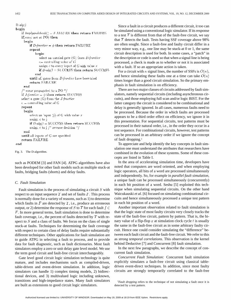
Fig. 3. The D-algorithm.
such as PODEM [3] and FAN [4]. ATPG algorithms have alsobeen developed for other fault models such as multiple stuck-atfaults, bridging faults (shorts) and delay faults.
C. Fault Simulation
Fault simulation is the process of simulating a circuitwithrespect to an input sequenceand set of faults . This processis normally done for a variety of reasons, such as 1) to determinewhich faults in are detected by , i.e., produce an erroneousoutput, or 2) determine the response ofto for each fault
. In more general terms, fault simulation is done to determinefault coverage, i.e., the percent of faults detected bywith re-spect to and a class of faults. We focus on the class of singlestuck-at faults. Techniques for determining the fault coveragewith respect to certain class of delay faults require substantiallydifferent techniques. Other applications for fault simulation areto guide ATPG in selecting a fault to process, and to providedata for fault diagnostic, such as fault dictionaries. Most faultsimulators employ a zero or unit delay gate level model. We usethe term good circuit and fault-free circuit interchangeably.
Gate level good circuit logic simulation technology is quitemature, and includes mechanisms such as compiled-driven,table-driven and event-driven simulation. In addition, logicsimulators can handle 1) complex timing models, 2) bidirec-tional devices, and 3) multivalued logic including unknown,transitions and high-impedance states. Many fault simulatorsare built as extensions to good circuit logic simulators.
Since a fault in a circuit produces a different circuit, it too canbe simulated using a conventional logic simulator. If its responseto a test is different from that of the fault-free circuit, we saythat detects the fault. Tests having SSF coverage above 98%are often sought. Since a fault-free and faulty circuit differ in avery minor way, e.g., one line may be stuck-at 0 or 1, the samecircuit description is used for both. In some cases, a “patch” inthe description or code is used so that when a signal line is beingprocessed, a check is made as to whether or not it is associatedwith a fault. If so an appropriate action is taken.
For a circuit with signal lines, the number of SSFs is ,and hence simulating these faults one at a time can taketimes longer than a good circuit simulation. So the primary em-phasis in fault simulation is on efficiency.
There are two major classes of circuits addressed by fault sim-ulators, namely sequential circuits (including asynchronous cir-cuits), and those employing full scan and/or logic BIST. For thelatter category the circuit is considered to be combinational anddelay is generally ignored. In all cases, numerous faults need tobe processed. Because the order in which faults are processedappears to be a third order effect on efficiency, we ignore it inthis presentation. For sequential circuits, test patterns must beprocessed in their natural order, i.e., in the order they occur in atest sequence. For combinational circuits, however, test patternscan be processed in an arbitrary order if we ignore the conceptof fault dropping.1
To appreciate and help identify the key concepts in fault sim-ulation one must understand the attributes that researchers havecombined in the evolution of these systems. Some of these con-cepts are listed in Table I.
In the area of accelerating simulation time, developers havenoted that computers are word oriented, and when employinglogic operators, all bits of a word are processed simultaneouslyand independently. So, for example inparallel fault simulation,a unique fault can be processed simultaneously (concurrently)in each bit position of a word. Seshu [5] exploited this tech-nique when simulating sequential circuits. On the other handWaicukauskiet al.[6] focused on simulating combinational cir-cuits and hence simultaneously processed a unique test patternin each bit position of a word.
Another important observation related to fault simulation isthat the logic state of most faulty circuits very closely tracks thestate of the fault-free circuit, pattern by pattern. That is, the bi-nary value of a flip-flop at simulation clock cycle is usuallythe same in the fault-free circuit as in some arbitrary faulty cir-cuit. Hence one could consider simulating the “difference” be-tween each fault circuit and the fault-free circuit. We refer to thisasstrong temporal correlations. This observation is the kernelbehind Deductive [7] and Concurrent [8] fault simulation.
In the next few paragraphs, we describe the concept of con-current fault simulation.
Concurrent Fault Simulation:Concurrent fault simulationexplicitly simulates a fault-free circuit using classical table-driven event-direct techniques. In addition, since most faultycircuits are strongly temporarily correlated to the fault-free
1Fault droppingrefers to the technique of not simulating a fault once it isdetected by a test pattern.
Authorized licensed use limited to: UNIVERSITY OF WINDSOR. Downloaded on May 19, 2009 at 18:19 from IEEE Xplore. Restrictions apply.
BREUERet al.: FUNDAMENTAL CAD ALGORITHMS 1453
TABLE IA DESIGN SPACE FORFAULT SIMULATORS
Fig. 4. Example circuit.
circuit, they are simulatedimplicitly, i.e., events that occur inthe fault-free circuit also occur in most faulty circuits. Thosecases where this is not the case are simulatedexplicitly.
Let be a logic circuit and the same circuit except itcontains a fault in some signal line. We associate with eachelement in , such as a gate or flip-flop, aconcurrentfault list,denoted by . contains entries of the form ,where is a fault and is a set of signal values. Let denotethe replica or image of in . Note that in general is notrelated to . For example, referring to Fig. 4, fault defines acircuit , and the image of gate in this circuit is .
Let denote the ensemble of input, output, andpossibly internal state values of . Note that if were aflip-flop or register it would have a state. A faultis said to bea local fault of if it is associated with either an input, output,or state of . Referring to Fig. 4, the local faults of are ,
, , , , and . At a specific point in simulation time,assume the signal values are as shown in Fig. 4. In the faultfree circuit, gate would be associated with the pair ,where , were the fault-freecircuit is denoted by the index zero. The elementwould beassociated with several entities, including the local fault entries
, and , where the fault forcesline to a one. The path – – is a sensitized path, andthere exist one stuck-at fault on each segment of this path thatis detected by the input pattern.
During simulation contains the set of all elementsthat differ from at the current simulated time. If ,then . Also, if is a local fault of , then
even if .A fault is said to bevisibleon a line when the valuein anddiffer. Concurrent simulation employs the concept of events
and simulation is primary involved in updating the dynamic datastructures and processing the concurrent fault lists.
The initial content of each consists of entries corre-sponding to the local faults of. Concurrent simulation nor-mally employs fault dropping and, thus, local faults ofremain
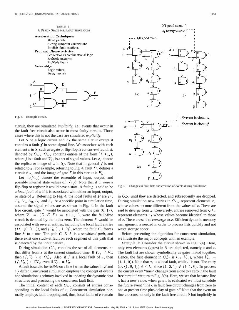
Fig. 5. Changes in fault lists and creation of events during simulation.
in until they are detected, and subsequently are dropped.During simulation new entries in represent elementswhose values become different from the values of. These aresaid todivergefrom . Conversely, entries removed fromrepresent elements whose values become identical to thoseof . These are said toconvergeto . Efficient dynamic memorymanagement is needed in order to process lists quickly and notwaste storage space.
Before presenting the algorithm for concurrent simulation,we illustrate the major concepts with an example.
Example 3: Consider the circuit shown in Fig. 5(a). Here,only two elements (gates) in are depicted, namely and .The fault list are shown symbolically as gates linked together.Hence, the first element in is , where
. Note that is a local fault, while is not. The entrysince . To process
the current event “line changes from a one to a zero in the faultfree circuit,” we turn to Fig. 5(b). Here, we see that because line
has a new value, when gateis evaluated we must schedulethe future event “line in fault free circuit changes from zero toone at present time plus delay of gate.” Note that the event online occurs not only in the fault free circuit but implicitly in
Authorized licensed use limited to: UNIVERSITY OF WINDSOR. Downloaded on May 19, 2009 at 18:19 from IEEE Xplore. Restrictions apply.
1454 IEEE TRANSACTIONS ON COMPUTER AIDED DESIGN OF INTEGRATED CIRCUITS AND SYSTEMS, VOL. 19, NO. 12, DECEMBER 2000
Fig. 6. Elements A and B.
all fault circuits that do not have entries in . The entries inare processed explicitly. Note that the event on linedoes
not effect the first entry in , since it corresponds to line– –1. Evaluating the entry corresponding to gatedoes not
result in a new event since the output of gateand will bethe same once is updated.
When the value of is eventually updated, fault is identi-fied as being newly visible on line.
The good event on line does not produce an event on line. As seen in Fig. 5(c), the newly visible fault produces an
entry in . The new value of also produces the followingchanges to : for entry , the output changes from oneto zero that in turn produces an event tied to only. It is,thus, seen that there are two types of events, namely good circuitevents that apply to not only the fault-free circuit but also allfaulty circuits, except for those that attempt to set a line that is– – to a value other than, and events that are specific to a
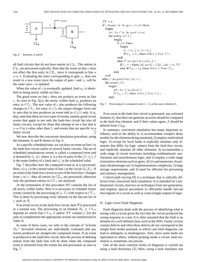
faulty circuit.We now describe the concurrent simulation procedure, using
the elements A and B shown in Fig. 6.At a specific scheduled time, we can have an event on linein
the fault-free circuit and/or in several faulty circuits. The set ofscheduled simultaneous events is called acomposed eventandis denoted by , where is a list of pairs of the ,is the name (index) of a fault and is the scheduled value.
Fig. 7 describes how the composed event atis processed.Here, is the current value of linein the circuit . Ifan event in the fault-free circuit occurs of the form linechangesfrom to , then all entries in are processed; otherwiseonly the pertinent entries in are analyzed.
At the termination of this procedure NV contains the list ofall newly visible faults. Next it is necessary to schedule futureevents created by the processing of with respect to .This is done by processing every element on the fan-out list of, such as .
If an event occurs in the fault-free circuit, thenis processedin a normal way. The processing of an elementdepends on which lists , and/or contain . For thesake of completeness the appropriate actions are summarized inTable II.
In some of these cases, we refer to the concept of “activate.” Activated elementsare individually evaluated and any
events produced are merged into composed events. If an eventis produced in the fault-free circuit, then the process of deletingentries from the fault lists will be done when the composedevent is retrieved from the events list and processed, as seen inFig. 7.
Fig. 7. Processing of a composed event(i; L) at the source element A.
If no event in the fault-free circuit is generated, any activatedelement that does not generate an event should be comparedto the fault-free element, and if their values agree,should bedeleted from .
In summary, concurrent simulation has many important at-tributes, such as the ability to 1) accommodate complex delaymodels for the elements being simulated, 2) employ multivaluedlogic; 3) except for local faults it explicitly simulate only el-ements that differ (in logic values) from the fault-free circuit,and implicitly simulate all other elements; 4) accommodate awide range of circuit structures including combinational, syn-chronous and asynchronous logic, and 5) employ a wide rangeof primitive elements such as gates, ALUs and memories. Its pri-mary disadvantages are 1) implementations complexity, 2) largestorage requirements, and 3) need for efficient list processingand memory management.
Critical path tracing [9] is a technique that is radically dif-ferent from concurrent fault simulation. It is intended for com-binational circuits, borrows on techniques from test generation,and employs special procedures to efficiently handle fan-outfree regions of a circuit as well as cones (single output) of logic.
D. Logic-Level Fault Diagnosis
Fault diagnosis deals with the process of identifying what iswrong with a circuit given the fact that the circuit produced thewrong response to a test. It is often assumed that the fault is anelement of a well-defined class, such as the SSFs. Faulty circuitscontain defects and often these defects do not correspond to thesimple fault model assumed, in which case fault diagnosis canlead to ambiguity or misdiagnosis. Also, since some faults areequivalent to others, without probing inside a circuit, fault res-olution is sometimes not precise.
One of the most common forms of diagnosis is carried outusing a fault dictionary [5]. Here, using a fault simulator one
Authorized licensed use limited to: UNIVERSITY OF WINDSOR. Downloaded on May 19, 2009 at 18:19 from IEEE Xplore. Restrictions apply.
BREUERet al.: FUNDAMENTAL CAD ALGORITHMS 1455
TABLE IIPROCESSINGELEMENT B 2 CL
can build an array indicating test pattern number, fault number(index) and response. Given the response from a circuit undertest (CUT) one can search this dictionary for a match whichthen indicates the fault. This diagnostic methodology leads tovery large dictionaries and is not applicable to multiple faults.This form of diagnosis is referred to ascause–effect analysis,where the possible causes (faults) lead to corresponding effects(responses). The faults are explicitly enumerated prior to con-structing the fault dictionary.
Effect–Cause Analysis:In this section, we briefly describethe effect–cause analysismethodology [10], [11]. This diag-nosis technique has the following attributes: 1) it implicitly em-ploys a multiple stuck-at fault model and, thus, does not enu-merate faults; 2) it identifies faults to within equivalence classes;and 3) it does not require fault simulation or even the responsefrom the fault-free circuit.
Let be a model of a fault-free circuit, an instance ofbeing tested, the test sequence, and the response of
to . In effect-cause analysis, we process the actual re-sponse (the effect) to determine the faults in (the cause).The response is not used. Effect-cause analysis consists oftwo phases. In the first phase, one executes theDeduction Algo-rithm, where the internal signal values in are deduced. In thesecond phase, one identifies the status of lines in, i.e., whichare fault-free or normal , which only take on the values 0 or1, and which cannot be– –0 or – –1, denoted by and ,respectively.
Note that by carrying out a test where only the primary outputlines are observable, it is not feasible to always identify a faultto a specific line. This occurs for reasons such as fault equiva-lence and fault masking. A few examples will help clarify thecomplexity of this problem.
Example 4: Consider a single output cone of logic .
a) If the output line is – – , where , then all otherfaults in are masked, i.e., cannot be identified by aninput/output (I/O) experiment and have no impact on theoutput response.
b) Assume the output is driven by anAND gate. Then anyinput line to this gate that is– –0 is equivalent (indis-tinguishable) from the output– –0 as well as any otherinput – –0.
Effect–cause analysis relies on many theoretical properties oflogic circuits, several of which were first identified during theevolution of this work. We next list those results that are mostimportant for understanding the development and correctness ofthe Deduction Algorithm.
We assume a line in is either normal, – –0 or – –1. Anormal pathis a sequence of normal lines separated by fault-freegates.
• (Normal Path): The logic values of an internal linecanbe deduced from an I/O experiment only if there exists atleast one normal path connectingwith some PO.
We assume a natural lexicographic ordering of the lines inand of test patterns in . Therefore, we do not distinguish
between a signal lineand the th line in a circuit, nor the testpattern and the th test pattern.
Let be the value of signal linein when test patternis applied.
Let matrix . In , the signal values are denoted by.
• (PO): If line is – – , , then .• (P1): Let be the output of gate. If is normal then for
all , and the values of the inputs tomust covera primitive cube of .
• (P2): If is a fan-out branch (FOB) of, then lines andhave the same values in every test.
• (P3): If line is a normal , then .• (P4): Consider the basic primitive gatesAND, OR, NAND,
NOR, andINVERTER. Then for every pair of primitive cubesin which the output of a gate has complementary values,there exists an input with complementary values.
• (Complete Normal Path): If a P0 line has comple-mentary values in and , then there exists at least onecomplete normal path in between some and ,and every line on this path has complementary values inand .
The process of analyzing and results in conclusions thatare referred to asforced-values( s). Determining forcedvalues is similar to carrying out an implication process basedon . Forced values are determined as a preprocessing step tothe Deduction Algorithm.
Definition 1: Line hasproperty in test , where, iff either or else . A shorthand
notation for this concept is to write .
• (P5): For every , , i.e., the ex-pected values of a are its s.
• (P6): If is a FOB of , then , i.e.,a fan-out branch has the s of its stem.
• (P7): Let be the output of a noninverting (inverting)gate having inputs . Then iff
for .Here, we see that we can deduce information about the output
of a gate if all the inputs of the gate have for test .
Authorized licensed use limited to: UNIVERSITY OF WINDSOR. Downloaded on May 19, 2009 at 18:19 from IEEE Xplore. Restrictions apply.
1456 IEEE TRANSACTIONS ON COMPUTER AIDED DESIGN OF INTEGRATED CIRCUITS AND SYSTEMS, VOL. 19, NO. 12, DECEMBER 2000
Fig. 8. (a) Circuit to be analyzed. (b) Expected values. (c) Forced values.
Notation: Let be the set of tests in whichhas , i.e.,.
• (P8): If for some , , then .This result represent vertical (between tests) implicationand will be illustrated later.
Properties P5–P7 allow one to determines at the s andmove s forward through a circuit.
As stated previously, if , then has propertyin test independent of the fault situation in and, thus, in-dependent of the status of other lines in. However, there aresituations when the status of a line may depend on the valueof other lines. This leads to the concept of conditional forcedvalues ( s) [10].
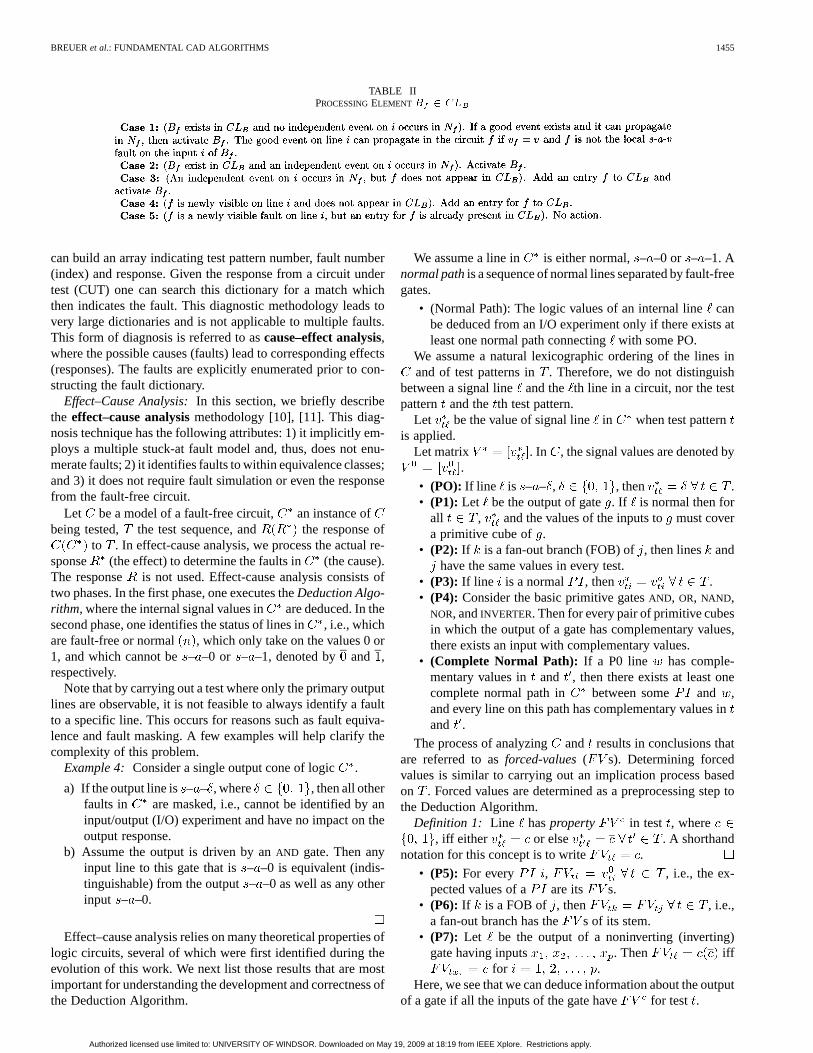
Example 5: Consider the circuit shown in Fig. 8(a). InFig. 8(b), we show the expected (fault-free) values in responseto the test . While only the values applied at
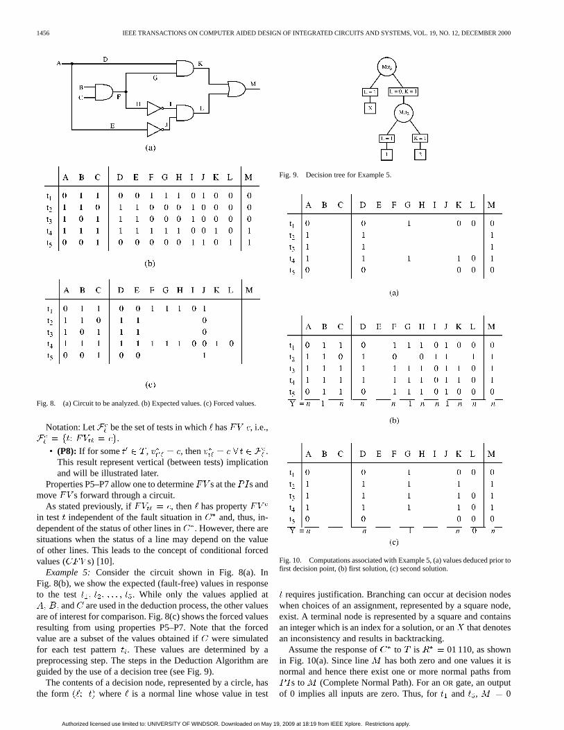
and are used in the deduction process, the other valuesare of interest for comparison. Fig. 8(c) shows the forced valuesresulting from using properties P5–P7. Note that the forcedvalue are a subset of the values obtained ifwere simulatedfor each test pattern . These values are determined by apreprocessing step. The steps in the Deduction Algorithm areguided by the use of a decision tree (see Fig. 9).
The contents of a decision node, represented by a circle, hasthe form where is a normal line whose value in test
Fig. 9. Decision tree for Example 5.
Fig. 10. Computations associated with Example 5, (a) values deduced prior tofirst decision point, (b) first solution, (c) second solution.
requires justification. Branching can occur at decision nodeswhen choices of an assignment, represented by a square node,exist. A terminal node is represented by a square and containsan integer which is an index for a solution, or anthat denotesan inconsistency and results in backtracking.
Assume the response of to is 01 110, as shownin Fig. 10(a). Since line has both zero and one values it isnormal and hence there exist one or more normal paths from
s to (Complete Normal Path). For anOR gate, an outputof 0 implies all inputs are zero. Thus, for and , 0
Authorized licensed use limited to: UNIVERSITY OF WINDSOR. Downloaded on May 19, 2009 at 18:19 from IEEE Xplore. Restrictions apply.
BREUERet al.: FUNDAMENTAL CAD ALGORITHMS 1457
implies 0. Since has in and a 0 valuehas been deduced for (in and ), then 0 in . Thisis an example of avertical implication , i.e., values in one testimplying line values in another test. This concept is unique tothe deduction algorithm. Knowing 0 and 1 inimplies 1 since is anOR gate. This is an example ofhorizontal implication . Thus, is normal! Continuing,1 in implies 1 and 1 in , which generate thevertical implications 1 in and , and 1 in . Now
in implies 0 in , which implies 0 in . Atthis point all the values of D can be assigned to its stem A (P2).No more implications exists.
We next attempt to justify the value of in and . We firstselect as shown in the decision tree in Fig. 9. We initially trythe assignment 1. Carrying out the resulting implicationsresults in a conflict, i.e., line is assigned both a zero and a one.Since in this analysis, we can reverse our decision andset 0 and 1 as our next decision (see decision tree).Going from the terminal node labeled and the new decisionnode is done via backtracking. Now 1 in implies1 in . Again there are no more implications possible, so a newdecision node is created, labeled . The two assignments
1 lead to two solutions shown in Fig. 10(b) and (c),respectively.
Note that lines and are identified as beingnormal with respect to the first solution only. The lines
, and are normal in both solutions and, therefore,are actually normal (fault-free) lines in . Note also that
designate a path between a and a .The reader is referred to [10] and [12] for details of the De-
duction Algorithm.The second phase of effect–cause analysis deals with deter-
mining the states of the lines in . A complete analysis of themapping of the results generated by the Deduction Algorithm topotential failures in is again beyond the scope of this paper.A brief overview, however, will be presented.
We represent the statusof a line by zero, one, or , wherezero(one) represents– –0(1), and represents normal. Thena fault situationis defined by the vector . Recall that
is the fault free circuit. Let denote the circuit in thepresence of fault situation . Clearly, ifthen . realizes the Boolean switching function .If then we say that and are indistinguish-able. Let . Thus, the fault situa-tions can be partitioned into equivalence classes. The faults in
are undetectable and, therefore, redun-dant. Let be the response of to . Then we say that
and areequivalent under iff . Let. Our goal in fault analysis (phase 2)
is to identify one or more members of the set. For each so-lution generated by the deduction algorithm we derive akernelfault that corresponds (covers) a family of faults that may ac-tually exist in . Let be a kernel fault, where
, and means that the state ofis unknown.Note that and have the same meaning asand . can be constructed as follows: 1) iff both zeroand one values have been deduced for; 2) iff onlyzero(one) values have been deduced for, and 3) iff
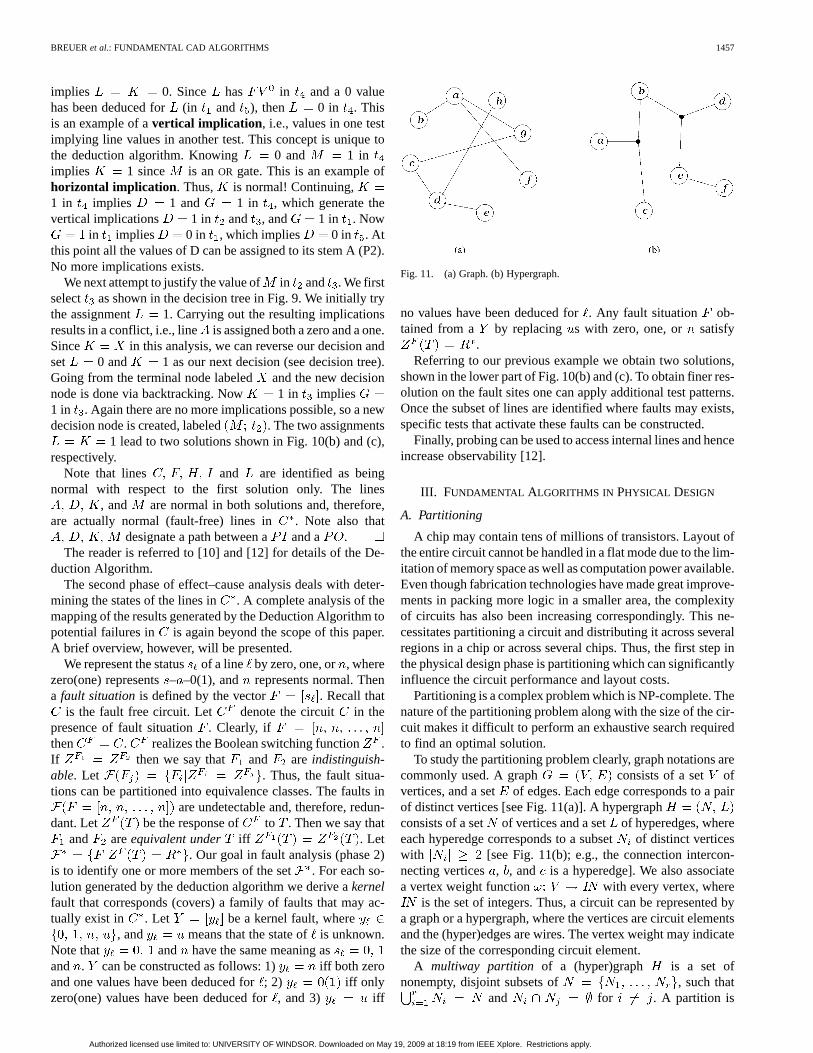
Fig. 11. (a) Graph. (b) Hypergraph.
no values have been deduced for. Any fault situation ob-tained from a by replacing s with zero, one, or satisfy
.Referring to our previous example we obtain two solutions,
shown in the lower part of Fig. 10(b) and (c). To obtain finer res-olution on the fault sites one can apply additional test patterns.Once the subset of lines are identified where faults may exists,specific tests that activate these faults can be constructed.
Finally, probing can be used to access internal lines and henceincrease observability [12].
III. FUNDAMENTAL ALGORITHMS IN PHYSICAL DESIGN
A. Partitioning
A chip may contain tens of millions of transistors. Layout ofthe entire circuit cannot be handled in a flat mode due to the lim-itation of memory space as well as computation power available.Even though fabrication technologies have made great improve-ments in packing more logic in a smaller area, the complexityof circuits has also been increasing correspondingly. This ne-cessitates partitioning a circuit and distributing it across severalregions in a chip or across several chips. Thus, the first step inthe physical design phase is partitioning which can significantlyinfluence the circuit performance and layout costs.
Partitioning is a complex problem which is NP-complete. Thenature of the partitioning problem along with the size of the cir-cuit makes it difficult to perform an exhaustive search requiredto find an optimal solution.
To study the partitioning problem clearly, graph notations arecommonly used. A graph consists of a set ofvertices, and a set of edges. Each edge corresponds to a pairof distinct vertices [see Fig. 11(a)]. A hypergraphconsists of a set of vertices and a set of hyperedges, whereeach hyperedge corresponds to a subsetof distinct verticeswith [see Fig. 11(b); e.g., the connection intercon-necting vertices , , and is a hyperedge]. We also associatea vertex weight function with every vertex, where
is the set of integers. Thus, a circuit can be represented bya graph or a hypergraph, where the vertices are circuit elementsand the (hyper)edges are wires. The vertex weight may indicatethe size of the corresponding circuit element.
A multiway partition of a (hyper)graph is a set ofnonempty, disjoint subsets of , such that
and for . A partition is
Authorized licensed use limited to: UNIVERSITY OF WINDSOR. Downloaded on May 19, 2009 at 18:19 from IEEE Xplore. Restrictions apply.
1458 IEEE TRANSACTIONS ON COMPUTER AIDED DESIGN OF INTEGRATED CIRCUITS AND SYSTEMS, VOL. 19, NO. 12, DECEMBER 2000
acceptableif , where is the sum ofthe weight of vertices in , is the maximum size of partand is the minimum size of part, for ; sand s are input parameters. A special case of multiwaypartitioning problem in which 2 is called thebipartitionproblem. In the bipartition problem, is at least times thesum of the weight of all vertices, for some, .Typically, is close to 1/2. The numberis called thebalancefactor. The bipartition problem can also be used as a basis forheuristics in multiway partitioning. Normally, the objectiveis to minimize the number ofcut edge, that is, the number ofhyperedges with at least one vertex in each partition.
Classic iterative approaches known Kernighan–Lin (KL) andFiduccia–Mattheyses (FM) begin with some initial solution andtry to improve it by making small changes, such as swappingmodules between clusters. Iterative improvement has becomethe industry standard for partitioning due to its simplicity andflexibility. Recently, there have been many significant improve-ments to the basic FM algorithm. Multilevel approaches are verypopular and produce superior partitioning results for very largesized circuits. In this section, we discuss the basic FM algorithmand hMetis, a multilevel partitioning algorithm, which is one ofthe best partitioners.
The KL and FM Algorithms:To date, iterative improvementtechniques that make local changes to an initial partition arestill the most successful partitioning algorithms in practice. Onesuch algorithm is an iterative bipartitioning algorithm proposedby Kernighan and Lin [13].
Given an unweighted graph , this method startswith an arbitrary partition of into two groups and suchthat and , where is the bal-ance factor as defined in the previous subsection andde-notes the number of vertices in set. A passof the algorithmstarts as follows. The algorithm determines the vertex pair (,
), and , whose exchange results in the largestdecrease of the cut-cost or in the smallest increase if no decreaseis possible. A cost increase is allowed now in the hope that therewill be a cost decrease in subsequent steps. Then the verticesand are locked. This locking prohibits them from taking partin any further exchanges. This process continues, keeping a listof all tentatively exchanged pairs and the decreasing gain (orcut-cost), until all the vertices are locked.
A value is selected to maximize the partial sumGain , where is the gain of the th ex-
changed pair. If Gain , a reduction in cut-cost can beachieved by moving to andto . This marks the end of one pass. The resulting partition istreated as the initial partition, and the procedure is repeated forthe next pass. If there is nosuch that Gain the procedurehalts. A formal description of KL algorithm is as follows.
Procedure: KL heuristic( );begin-1
bipartition into two groups and, with ;
repeat-2for do
begin-3find a pair of unlocked vertices
and whose exchangemakes the largest decrease orsmallest increase in cut-cost;
mark , as locked and storethe gain ;end-3
find , such thatis maximized;
if thenmove from to and
from to ;until-2 ;
end-1.
The for-loop is executed times. The body of the looprequires time. Thus, the total running time of the algo-rithm is for each pass of the repeat loop. The repeat loopusually terminates after several passes, independent of. Thus,the total running time is , where is the number of timesthe repeat loop is executed.
Fiduccia and Mattheyses [14] improved the Kernighan-Linalgorithm by reducing the time complexity per pass to ,where is the number of hyper-edge ends (or,terminals) in .FM added the following new elements to the KL algorithm:
1) only a single vertex is moved across the cut in a singlemove;
2) adding weights to vertices;3) a special data structure for selecting vertices to be moved
across the cut to improve running time (this is the mainfeature of the algorithm).
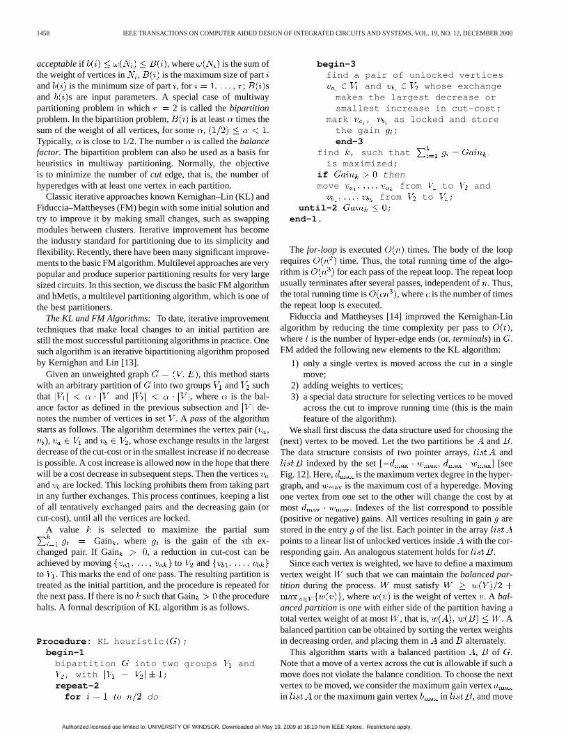
We shall first discuss the data structure used for choosing the(next) vertex to be moved. Let the two partitions beand .The data structure consists of two pointer arrays, and
indexed by the set [ ] [seeFig. 12]. Here, is the maximum vertex degree in the hyper-graph, and is the maximum cost of a hyperedge. Movingone vertex from one set to the other will change the cost by atmost . Indexes of the list correspond to possible(positive or negative) gains. All vertices resulting in gainarestored in the entry of the list. Each pointer in the arraypoints to a linear list of unlocked vertices insidewith the cor-responding gain. An analogous statement holds for .
Since each vertex is weighted, we have to define a maximumvertex weight such that we can maintain thebalanced par-tition during the process. must satisfy
, where is the weight of vertex . A bal-anced partitionis one with either side of the partition having atotal vertex weight of at most , that is, . Abalanced partition can be obtained by sorting the vertex weightsin decreasing order, and placing them inand alternately.
This algorithm starts with a balanced partition, of .Note that a move of a vertex across the cut is allowable if such amove does not violate the balance condition. To choose the nextvertex to be moved, we consider the maximum gain vertexin or the maximum gain vertex in , and move
Authorized licensed use limited to: UNIVERSITY OF WINDSOR. Downloaded on May 19, 2009 at 18:19 from IEEE Xplore. Restrictions apply.
BREUERet al.: FUNDAMENTAL CAD ALGORITHMS 1459
Fig. 12. The data structure for choosing vertices in FM algorithm.
them across the cut if the balance condition is not violated. Asin the KL algorithm, the moves are tentative and are followedby locking the moved vertex. A move may increase the cut-cost.When no moves are possible or if there are no more unlockedvertices, choose the sequence of moves such that the cut-cost isminimized. Otherwise the pass is ended.
Further improvement was proposed by Krishnamurthy [15].He introduced alook-aheadability to the algorithm. Thus, thebest candidate among such vertices can be selected with respectto the gains they make possible in later moves.
In general, the obtained bipartition from KL or FM algorithmis a local optimum rather than a global optimum. The perfor-mance of KL–FM algorithm degrades severely as the size of cir-cuits grows. However, better partitioning results can be obtainedby using clustering techniques and/or better initial partitions to-gether with KL-FM algorithm. The KL–FM algorithm (and itsvariations) are still the industry standard partitioning algorithmdue to its flexibility and the ability of handling very large cir-cuits.
hMetis—A Multilevel Partitioning Algorithm:Two-levelpartitioning approaches consist of two phases. In the first phase,the hypergraph is coarsened to form a small hypergraph, andthen the FM algorithm is used to bisect the small hypergraph. Inthe second phase, they use the bisection of this contracted hy-pergraph to obtain a bisection of the original hypergraph. SinceFM refinement is done only on the small coarse hypergraph,this step is usually fast. However, the overall performanceof such a scheme depends on the quality of the coarseningmethod. In many schemes, the projected partition is furtherimproved using the FM refinement scheme.
Multilevel partitioning approaches are developed to cope withlarge sized circuits [16]–[18]. In these approaches, a sequenceof successively smaller (coarser) graph is constructed. A bisec-tion of the smallest graph is computed. This bisection is nowsuccessively projected to the next level finer graph, and at eachlevel an iterative refinement algorithm such as KL–FM is used to
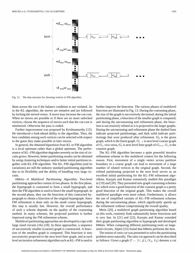
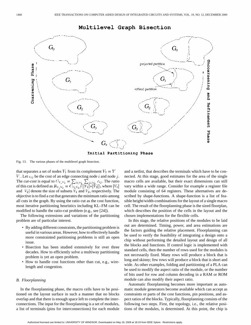
further improve the bisection. The various phases of multilevelbisection are illustrated in Fig. 13. During the coarsening phase,the size of the graph is successively decreased; during the initialpartitioning phase, a bisection of the smaller graph is computed;and during the uncoarsening and refinement phase, the bisec-tion is successively refined as it is projected to the larger graphs.During the uncoarsening and refinement phase the dashed linesindicate projected partitionings, and dark solid indicate parti-tionings that were produced after refinement. is the givengraph, which is the finest graph. is next level coarser graphof , vice versa, is next level finer graph of . is thecoarsest graph.
The KL–FM algorithm becomes a quite powerful iterativerefinement scheme in this multilevel context for the followingreason. First, movement of a single vertex across partitionboundary in a coarse graph can lead to movement of a largenumber of related vertices in the original graph. Second, therefined partitioning projected to the next level serves as anexcellent initial partitioning for the KL–FM refinement algo-rithms. Karypis and Kumar extensively studied this paradigmin [19] and [20]. They presented new graph coarsening schemesfor which even a good bisection of the coarsest graph is a prettygood bisection of the original graph. This makes the overallmultilevel paradigm even more robust. Furthermore, it allowsthe use of simplified variants of KL–FM refinement schemesduring the uncoarsening phase, which significantly speeds upthe refinement without compromising the overall quality.
Metis [20], a multilevel graph partitioning algorithm basedon this work, routinely finds substantially better bisections andis very fast. In [21] and [22], Karypis and Kumar extendedtheir graph partitioning algorithm to hypergraph and developedhMetis. When comparing different partitioning tools on large-sized circuits, Alpert [23] found that hMetis performs the best.
The notion ofratio cutwas presented to solve the partitioningproblem more naturally. The ratio cut approach can be describedas follows: Given a graph , denotes a cut
Authorized licensed use limited to: UNIVERSITY OF WINDSOR. Downloaded on May 19, 2009 at 18:19 from IEEE Xplore. Restrictions apply.
1460 IEEE TRANSACTIONS ON COMPUTER AIDED DESIGN OF INTEGRATED CIRCUITS AND SYSTEMS, VOL. 19, NO. 12, DECEMBER 2000
Fig. 13. The various phases of the multilevel graph bisection.
that separates a set of nodesfrom its complement. Let be the cost of an edge connecting nodeand node .
Thecut-costis equal to . Theratioof this cut is defined as , whereand denote the size of subsets and , respectively. Theobjective is to find a cut that generates the minimum ratio amongall cuts in the graph. By using the ratio cut as the cost function,most iterative partitioning heuristics including KL–FM can bemodified to handle the ratio-cut problem (e.g., see [24]).
The following extensions and variations of the partitioningproblem are of particular interest.
• By adding different constraints, the partitioning problem isuseful in various areas. However, how to effectively handlemore constrainted partitioning problems is still an openissue.
• Bisection has been studied extensively for over threedecades. How to efficiently solve a multiway partitioningproblem is yet an open problem.
• How to handle cost functions other than cut, e.g., wire-length and congestion.
B. Floorplanning
In the floorplanning phase, the macro cells have to be posi-tioned on the layout surface in such a manner that no blocksoverlap and that there is enough space left to complete the inter-connections. The input for the floorplanning is a set of modules,a list of terminals (pins for interconnections) for each module
and a netlist, that describes the terminals which have to be con-nected. At this stage, good estimates for the area of the singlemacro cells are available, but their exact dimensions can stillvary within a wide range. Consider for example a register filemodule consisting of 64 registers. These alternatives are de-scribed by shape-functions. A shape-function is a list of fea-sible height/width-combinations for the layout of a single macrocell. The result of the floorplanning phase is the sized floorplan,which describes the position of the cells in the layout and thechosen implementations for the flexible cells.
In this stage, the relative positions of the modules to be laidout are determined. Timing, power, and area estimations arethe factors guiding the relative placement. Floorplanning canbe used to verify the feasibility of integrating a design onto achip without performing the detailed layout and design of allthe blocks and functions. If control logic is implemented withstandard cells, then the number of rows used for the modules isnot necessarily fixed. Many rows will produce a block that islong and skinny; few rows will produce a block that is short andwide. As other examples, folding and partitioning of a PLA canbe used to modify the aspect ratio of the module, or the numberof bits used for row and column decoding in a RAM or ROMmodule can also modify their aspect ratio.
Automatic floorplanning becomes more important as auto-matic module generators become available which can accept asconstraints or parts of the cost functions, pin positions, and as-pect ratios of the blocks. Typically, floorplanning consists of thefollowing two steps. First, the topology, i.e., the relative posi-tions of the modules, is determined. At this point, the chip is
Authorized licensed use limited to: UNIVERSITY OF WINDSOR. Downloaded on May 19, 2009 at 18:19 from IEEE Xplore. Restrictions apply.
BREUERet al.: FUNDAMENTAL CAD ALGORITHMS 1461
viewed as a rectangle and the modules are the (basic) rectangleswhose relative positions are fixed. Next, we consider theareaoptimization problem, i.e., we determine a set of implementa-tions (one for each module) such that the total area of the chipis minimized. The topology of a floorplan is obtained by recur-sively using circuit partitioning techniques. Apartition dividesa given circuit into parts such that: 1) the sizes of thepartsare as close as possible and 2) the number of nets connecting the
parts is minimized. If 2, a recursive bipartition generates aslicing floorplan. A floorplan is slicing if it is either a basic rec-tangle or there is a line segment (called slice) that partitions theenclosing rectangle into two slicing floorplans. A slicing floor-plan can be represented by aslicing tree. Each leaf node of theslicing tree corresponds to a basic rectangle and each nonleafnode of the slicing tree corresponds to a slice.
There exist many different approaches to the floorplanningproblem. Wimeret al. [25] described a branch-and-bound ap-proach for the floorplan sizing problem, i.e., finding an optimalcombination of all possible layout-alternatives for all modulesafter placement. While their algorithm is able to find the best so-lution for this problem, it is very time consuming, especially forreal problem instances. Cohoonet al. [26] implemented a ge-netic algorithm for the whole floorplanning problem. Their al-gorithm makes use of estimates for the required routing space toensure completion of the interconnections. Another widely usedheuristic solution method is simulated annealing [27], [28].
When the area of the floorplan is considered, the problem ofchoosing for each module the implementation which optimizesa given evaluation function is referred to as thefloorplan areaoptimization problem[29].
A floorplan consists of an enveloping rectangle partitionedinto nonoverlapping basic rectangles (or modules). For everybasic rectangle a set of implementations is given, which havea rectangular shape characterized by a widthand a height .The relative positions of the basic rectangles are specified by thefloorplan tree: the leaves are the basic rectangles,the root is theenveloping rectangle, and the internal nodes are thecompositerectangles. Each of the composite rectangles is divided intoparts in ahierarchical floorplanof order : if 2(slicingfloorplan), a vertical or horizontal line is used to partition therectangle; if 5, a right or leftwheelis obtained. The generalcase of composite blocks which cannot be partitioned in two orfive rectangles can be dealt with by allowing them to be com-posed of -shaped blocks. Once theimplementationfor eachblock has been chosen, the size of the composite rectangles canbe determined by traversing through upwards the floorplan tree;when the root is reached, the area of the enveloping rectanglecan be computed. The goal of the floorplan area optimizationproblem is to find the implementation for each basic rectanglesuch that the minimum area enveloping rectangle is obtained.The problem has been proven to be NP-complete in the generalcase, although it can be reduced to a problem solvable in poly-nomial time in the case of slicing floorplans.
Since floorplanning is done very early in the design process,only estimates of the area requirements for each module aregiven. Recently, the introduction of simulated annealing algo-rithms has made it possible to develop algorithms where the op-timization can be carried out with all the degrees of freedom
mentioned above. A system developed at the IBM T.J. WatsonResearch Center and use the simulated annealing algorithm toproduce a floorplan that not only gives the relative positions ofthe modules, but also aspect ratios and pin positions.
Simulated Annealing:Simulated annealing is a technique tosolve general optimization problems, floorplanning problemsbeing among them. This technique is especially useful whenthe solution space of the problem is not well understood. Theidea originated from observing crystal formation of materials.As a material is heated, the molecules move around in a randommotion. When the temperature slowly decreases, the moleculesmove less and eventually form crystalline structures. Whencooling is done in a slower manner, more crystal is at a min-imum energy state, and the material forms into a large crystallattice. If the crystal structure obtained is not acceptable, it maybe necessary to reheat the material and cool it at a slower rate.
Simulated annealing examines theconfigurations of theproblem in sequence. Each configuration is actually a feasiblesolution of the optimization problem. The algorithm movesfrom one solution to another, and a global cost function is usedto evaluate the desirability of a solution. Conceptually, we candefine aconfiguration graphwhere each vertex correspondsto a feasible solution, and a directed edge represents apossible movement from solution to .
The annealing process moves from one vertex (feasible solu-tion) to another vertex following the directed edges of the con-figuration graph. The random motion of the molecules at hightemperature is simulated by randomly accepting moves duringthe initial phases of the algorithm. As the algorithm proceeds,temperature decreases and it accepts less random movements.Regardless of the temperature, the algorithm will accept a move
if . When a local minimum isreached, all “small” moves lead to a higher cost solution. Toavoid being trapped in a local minimum, simulated annealingaccepts a movement to higher cost when the temperature is high.As the algorithm cools down, such movement is less likely tobe accepted. The best cost among all solutions visited by theprocess is recorded. When the algorithm terminates, hopefullyit has examined enough solutions to achieve a low cost solu-tion. Typically, the number of feasible solutions is an exponen-tial function of the problem size. Thus, the movement from onesolution to another is restricted to a very small fraction of thetotal configurations.
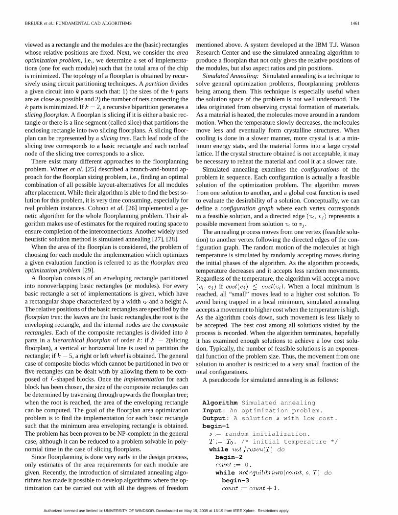
A pseudocode for simulated annealing is as follows:
Algorithm Simulated annealingInput : An optimization problem.Output : A solution with low cost.begin-1
random initialization.. /* initial temperature */
while dobegin-2
0.while do
begin-3.
Authorized licensed use limited to: UNIVERSITY OF WINDSOR. Downloaded on May 19, 2009 at 18:19 from IEEE Xplore. Restrictions apply.
1462 IEEE TRANSACTIONS ON COMPUTER AIDED DESIGN OF INTEGRATED CIRCUITS AND SYSTEMS, VOL. 19, NO. 12, DECEMBER 2000
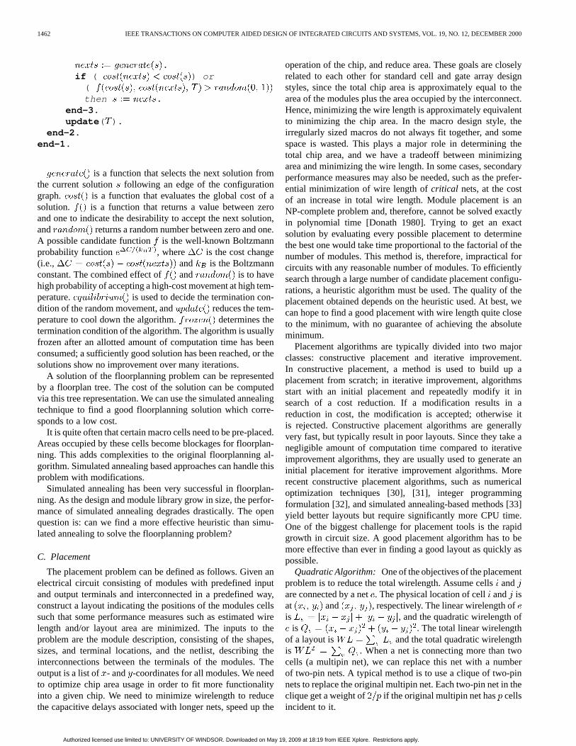
.if ( ) or
(then .
end-3 .update ( ).
end-2 .end-1 .
is a function that selects the next solution fromthe current solution following an edge of the configurationgraph. is a function that evaluates the global cost of asolution. is a function that returns a value between zeroand one to indicate the desirability to accept the next solution,and returns a random number between zero and one.A possible candidate function is the well-known Boltzmannprobability function , where is the cost change(i.e., and is the Boltzmannconstant. The combined effect of and is to havehigh probability of accepting a high-cost movement at high tem-perature. is used to decide the termination con-dition of the random movement, and reduces the tem-perature to cool down the algorithm. determines thetermination condition of the algorithm. The algorithm is usuallyfrozen after an allotted amount of computation time has beenconsumed; a sufficiently good solution has been reached, or thesolutions show no improvement over many iterations.
A solution of the floorplanning problem can be representedby a floorplan tree. The cost of the solution can be computedvia this tree representation. We can use the simulated annealingtechnique to find a good floorplanning solution which corre-sponds to a low cost.
It is quite often that certain macro cells need to be pre-placed.Areas occupied by these cells become blockages for floorplan-ning. This adds complexities to the original floorplanning al-gorithm. Simulated annealing based approaches can handle thisproblem with modifications.
Simulated annealing has been very successful in floorplan-ning. As the design and module library grow in size, the perfor-mance of simulated annealing degrades drastically. The openquestion is: can we find a more effective heuristic than simu-lated annealing to solve the floorplanning problem?
C. Placement
The placement problem can be defined as follows. Given anelectrical circuit consisting of modules with predefined inputand output terminals and interconnected in a predefined way,construct a layout indicating the positions of the modules cellssuch that some performance measures such as estimated wirelength and/or layout area are minimized. The inputs to theproblem are the module description, consisting of the shapes,sizes, and terminal locations, and the netlist, describing theinterconnections between the terminals of the modules. Theoutput is a list of - and -coordinates for all modules. We needto optimize chip area usage in order to fit more functionalityinto a given chip. We need to minimize wirelength to reducethe capacitive delays associated with longer nets, speed up the
operation of the chip, and reduce area. These goals are closelyrelated to each other for standard cell and gate array designstyles, since the total chip area is approximately equal to thearea of the modules plus the area occupied by the interconnect.Hence, minimizing the wire length is approximately equivalentto minimizing the chip area. In the macro design style, theirregularly sized macros do not always fit together, and somespace is wasted. This plays a major role in determining thetotal chip area, and we have a tradeoff between minimizingarea and minimizing the wire length. In some cases, secondaryperformance measures may also be needed, such as the prefer-ential minimization of wire length ofcritical nets, at the costof an increase in total wire length. Module placement is anNP-complete problem and, therefore, cannot be solved exactlyin polynomial time [Donath 1980]. Trying to get an exactsolution by evaluating every possible placement to determinethe best one would take time proportional to the factorial of thenumber of modules. This method is, therefore, impractical forcircuits with any reasonable number of modules. To efficientlysearch through a large number of candidate placement configu-rations, a heuristic algorithm must be used. The quality of theplacement obtained depends on the heuristic used. At best, wecan hope to find a good placement with wire length quite closeto the minimum, with no guarantee of achieving the absoluteminimum.
Placement algorithms are typically divided into two majorclasses: constructive placement and iterative improvement.In constructive placement, a method is used to build up aplacement from scratch; in iterative improvement, algorithmsstart with an initial placement and repeatedly modify it insearch of a cost reduction. If a modification results in areduction in cost, the modification is accepted; otherwise itis rejected. Constructive placement algorithms are generallyvery fast, but typically result in poor layouts. Since they take anegligible amount of computation time compared to iterativeimprovement algorithms, they are usually used to generate aninitial placement for iterative improvement algorithms. Morerecent constructive placement algorithms, such as numericaloptimization techniques [30], [31], integer programmingformulation [32], and simulated annealing-based methods [33]yield better layouts but require significantly more CPU time.One of the biggest challenge for placement tools is the rapidgrowth in circuit size. A good placement algorithm has to bemore effective than ever in finding a good layout as quickly aspossible.
Quadratic Algorithm: One of the objectives of the placementproblem is to reduce the total wirelength. Assume cellsandare connected by a net. The physical location of celland isat and , respectively. The linear wirelength ofis , and the quadratic wirelength of
is . The total linear wirelengthof a layout is and the total quadratic wirelengthis . When a net is connecting more than twocells (a multipin net), we can replace this net with a numberof two-pin nets. A typical method is to use a clique of two-pinnets to replace the original multipin net. Each two-pin net in theclique get a weight of if the original multipin net has cellsincident to it.
Authorized licensed use limited to: UNIVERSITY OF WINDSOR. Downloaded on May 19, 2009 at 18:19 from IEEE Xplore. Restrictions apply.
BREUERet al.: FUNDAMENTAL CAD ALGORITHMS 1463
Linear wirelength is widely used because it correlates wellwith the final layout area after routing. Quadratic wirelength isan alternative to use in placement. Experimental results showthat the quadratic wirelength objective over-penalizes longwires and has a worse correlation with the final chip area [34].However, since the quadratic wirelength objective is analytical,numerical methods can be used to solve for an optimal solution.The quadratic algorithm uses quadratic wirelength objectiveand analytical methods to generate a layout. It is very fast andleads to relatively good results.
Matrix representations and linear algebra are often used inquadratic placement algorithms. Assume the given circuit ismapped into a graph whereand . A nonnegative weight is as-signed to each edge . All the nets can be representedusing anadjacency matrix which has an entry
if and 0, otherwise. The physicallocations of all the vertices can be represented by-dimensionalvectors and , where is the coordi-nates of vertex .
The and directions are independent in quadratic wire-length objective. We can optimize the objective separately ineach direction. The following discussions will be focused on op-timizing the quadratic objective indirection. The same methodcan be used symmetrically in thedirection.
The total quadratic wirelength indirection of a given layoutcan be written as
(1)
is a Laplacian matrixof . has entry equalto if , and equal to otherwise, i.e., isthe degree of vertex . The optional linear term representsconnections of cells to fixed I/O pads. The vectorcan alsocapture pin offsets. The objective function (1) is minimized bysolving the linear system
(2)
The solution of this system of linear equations usually isnot a desired layout because vertices are not evenly distributed.This results in a lot of cell overlaps which are not allowed inplacement. A balanced vertex distribution in the placement areaneeds to be enforced. This can be achieved by either re-as-signing vertex locations after solving (2) or adding more con-straints to (1).
Existence of fixed vertices is essential for quadratic algo-rithms. Initially, I/O pads are fixed vertices. If no I/O pads arepresent, a trivial solution of (1) will be having all the verticeslocated at the same place. Existence of I/O pads forces verticesto separate to some extent. We can further spread the verticesto achieve a balanced distribution based on the solution of (2).This spreading procedure is based on heuristics and is not op-timal. Iterative approaches can be used to further improve thelayout. In the next iteration, a number of vertices can be fixed.A new layout can be obtained by solving a new equation similar
to (2). We can increase the number of fixed vertices graduallyor wait until this approach converges.
Constraints can also be added to (1) to help balance thevertex distribution. Researchers have added spatial constraintsso that the average location of different groups of vertices willbe evenly distributed in the placement area [30], [34], [35].They recursively reduce the number of vertices in vertex groupsby dividing them into smaller groups. Eisenmannet al. [36]added virtual spatial nets to (2). A virtual spatial net will havea negative weight if two cells incident to it are close to eachother. As two cells get closer, the absolute value of their spatialnet weight gets larger. The virtual spatial nets between cellstends to push overlapped cells further away from each otherdue to the negative weights. The weights on virtual spatial netsare updated each iteration until the solution converges.
The layouts produced by quadratic algorithm are not the bestcompared to layouts produced by other placement algorithms.The reason why quadratic algorithm is still attractive andwidely used in industry is because of its fast speed. It can rep-resent interactions between locations of cells and connectionsbetween cells using one simple linear equation (1). However, itneeds heuristics to balance the cell distribution in the placementarea. The effectiveness of these heuristics will highly affect thequality of the final layout.
Routing/congestion-driven placement aims to reduce thewiring congestion in the layout to ensure that the placementcan be routed using the given routing resources. Congestioncan be viewed using a supply-demand model [37]. Congestedregions are where the routing demand exceeds the routingresource supply. Wang and Sarrafzadeh [38] pointed out thatthe congestion is globally consistent with the wirelength.Thus, the traditional wirelength placement can still be used toeffectively reduce the congestion globally. However, in order toeliminate local congested spots in the layout, congestion-drivenapproaches are needed.
D. Routing
Routing is where interconnection paths are identified. Due tothe complexity, this step is broken into two stages: global anddetailed routing. In global routing, the “loose” routes for thenets are determined. For the computation of the global routing,the routing space is represented as a graph, the edges of thisgraph represent the routing regions and are weighted with thecorresponding capacities. Global routing is described by a listof routing regions for each net of the circuit, with none of thecapacities of any routing region being exceeded.
After global routing is done, for each routing region thenumber of nets routed is known. In the detailed routing phase,the exact physical routes for the wires inside routing regionshave to be determined. This is done incrementally, i.e., onechannel is routed at a time in a predefined order.
The problem of global routing is very much like a trafficproblem. The pins are the origins and destinations of traffic. Thewires connecting the pins are the traffic, and the channels arethe streets. If there are more wires than the number of tracks ina given channel, some of the wires have to be rerouted just likethe rerouting of traffic. For the real traffic problem, every driverwants to go to his destination in the quickest way, and he may try
Authorized licensed use limited to: UNIVERSITY OF WINDSOR. Downloaded on May 19, 2009 at 18:19 from IEEE Xplore. Restrictions apply.
1464 IEEE TRANSACTIONS ON COMPUTER AIDED DESIGN OF INTEGRATED CIRCUITS AND SYSTEMS, VOL. 19, NO. 12, DECEMBER 2000
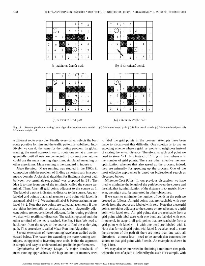
Fig. 14. An example demonstrating Lee’s algorithm from sources to sink t. (a) Minimum length path. (b) Bidirectional search. (c) Minimum bend path. (d)Minimum weight path.
a different route every day. Finally every driver selects the bestroute possible for him and the traffic pattern is stabilized. Intu-itively, we can do the same for the routing problem. In globalrouting, the usual approach was to route one net at a time se-quentially until all nets are connected. To connect one net, wecould use the maze running algorithm, simulated annealing orother algorithms. Maze running is the standard in industry.
Maze Running:Maze running was studied in the 1960s inconnection with the problem of finding a shortest path in a geo-metric domain. A classical algorithm for finding a shortest pathbetween two terminals (or, points) was proposed in [39]. Theidea is to start from one of the terminals, called the source ter-minal. Then,label all grid points adjacent to the source as 1.The label of a point indicates its distance to the source. Any un-labeled grid point that is adjacent to a grid point with labelisassigned label . We assign all labels before assigning anylabel . Note that two points are called adjacent only if theyare either horizontally or vertically adjacent; diagonally adja-cent points are not considered adjacent, for in routing problemswe deal with rectilinear distances. The task is repeated until theother terminal of the net is reached. See Fig. 14(a). We need tobacktrack from the target to the source to find the underlyingpath. This procedure is called Maze-Running Algorithm.
Several extensions of maze running have been studied as dis-cussed below. The reason for extending the maze running tech-niques, as opposed to inventing new tools, is that the approachis simple and easy to understand and predict its performance.
Optimization of Memory Usage:A major drawback ofmaze running approaches is the huge amount of memory used
to label the grid points in the process. Attempts have beenmade to circumvent this difficulty. One solution is to use anencoding scheme where a grid just points to neighbors insteadof storing the actual distance. Therefore, at each grid point weneed to store bits instead of bits, where isthe number of grid points. There are other effective memoryoptimization schemes that also speed up the process; indeed,they are primarily for speeding up the process. One of themost effective approaches is based on bidirectional search asdiscussed below.
Minimum-Cost Paths:In our previous discussion, we havetried to minimize the length of the path between the source andthe sink, that is, minimization of the distance inmetric. How-ever, we might also be interested in other objectives.
If we want to minimize the number of bends in the path weproceed as follows. All grid points that are reachable with zerobends from the source are labeled with zero. Note that these gridpoints are either adjacent to the source or are adjacent to a gridpoint with label zero. All grid points that are reachable from agrid point with label zero with one bend are labeled with one.In general, in stage, all grid points that are reachable from agrid point with label with one bend are labeled with.Note that for each grid point with label, we also need to storethe direction of the path (if there are more than one path, alldirections—at most four—need to be stored) that connects thesource to that grid point withbends. An example is shown inFig. 14(c).
We may also be interested in obtaining a minimum cost path,where the cost of a path is defined by the user. For example, with
Authorized licensed use limited to: UNIVERSITY OF WINDSOR. Downloaded on May 19, 2009 at 18:19 from IEEE Xplore. Restrictions apply.
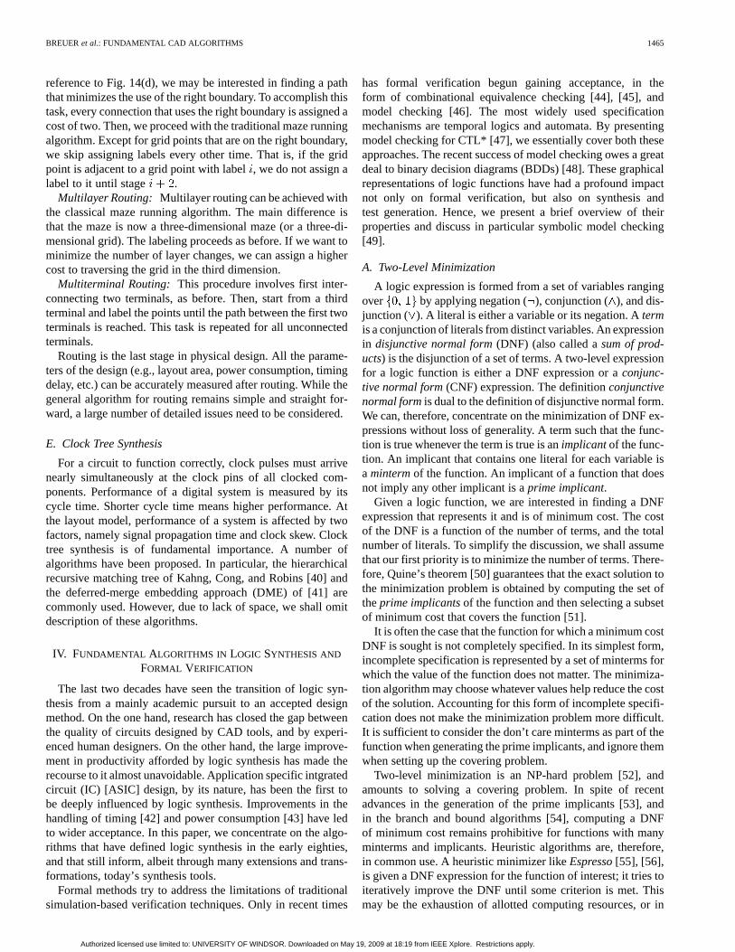
BREUERet al.: FUNDAMENTAL CAD ALGORITHMS 1465
reference to Fig. 14(d), we may be interested in finding a paththat minimizes the use of the right boundary. To accomplish thistask, every connection that uses the right boundary is assigned acost of two. Then, we proceed with the traditional maze runningalgorithm. Except for grid points that are on the right boundary,we skip assigning labels every other time. That is, if the gridpoint is adjacent to a grid point with label, we do not assign alabel to it until stage .
Multilayer Routing: Multilayer routing can be achieved withthe classical maze running algorithm. The main difference isthat the maze is now a three-dimensional maze (or a three-di-mensional grid). The labeling proceeds as before. If we want tominimize the number of layer changes, we can assign a highercost to traversing the grid in the third dimension.
Multiterminal Routing: This procedure involves first inter-connecting two terminals, as before. Then, start from a thirdterminal and label the points until the path between the first twoterminals is reached. This task is repeated for all unconnectedterminals.
Routing is the last stage in physical design. All the parame-ters of the design (e.g., layout area, power consumption, timingdelay, etc.) can be accurately measured after routing. While thegeneral algorithm for routing remains simple and straight for-ward, a large number of detailed issues need to be considered.
E. Clock Tree Synthesis
For a circuit to function correctly, clock pulses must arrivenearly simultaneously at the clock pins of all clocked com-ponents. Performance of a digital system is measured by itscycle time. Shorter cycle time means higher performance. Atthe layout model, performance of a system is affected by twofactors, namely signal propagation time and clock skew. Clocktree synthesis is of fundamental importance. A number ofalgorithms have been proposed. In particular, the hierarchicalrecursive matching tree of Kahng, Cong, and Robins [40] andthe deferred-merge embedding approach (DME) of [41] arecommonly used. However, due to lack of space, we shall omitdescription of these algorithms.
IV. FUNDAMENTAL ALGORITHMS IN LOGIC SYNTHESIS AND
FORMAL VERIFICATION
The last two decades have seen the transition of logic syn-thesis from a mainly academic pursuit to an accepted designmethod. On the one hand, research has closed the gap betweenthe quality of circuits designed by CAD tools, and by experi-enced human designers. On the other hand, the large improve-ment in productivity afforded by logic synthesis has made therecourse to it almost unavoidable. Application specific intgratedcircuit (IC) [ASIC] design, by its nature, has been the first tobe deeply influenced by logic synthesis. Improvements in thehandling of timing [42] and power consumption [43] have ledto wider acceptance. In this paper, we concentrate on the algo-rithms that have defined logic synthesis in the early eighties,and that still inform, albeit through many extensions and trans-formations, today’s synthesis tools.
Formal methods try to address the limitations of traditionalsimulation-based verification techniques. Only in recent times
has formal verification begun gaining acceptance, in theform of combinational equivalence checking [44], [45], andmodel checking [46]. The most widely used specificationmechanisms are temporal logics and automata. By presentingmodel checking for CTL* [47], we essentially cover both theseapproaches. The recent success of model checking owes a greatdeal to binary decision diagrams (BDDs) [48]. These graphicalrepresentations of logic functions have had a profound impactnot only on formal verification, but also on synthesis andtest generation. Hence, we present a brief overview of theirproperties and discuss in particular symbolic model checking[49].
A. Two-Level Minimization
A logic expression is formed from a set of variables rangingover by applying negation (), conjunction ( ), and dis-junction ( ). A literal is either a variable or its negation. Atermis a conjunction of literals from distinct variables. An expressionin disjunctive normal form(DNF) (also called asum of prod-ucts) is the disjunction of a set of terms. A two-level expressionfor a logic function is either a DNF expression or aconjunc-tive normal form(CNF) expression. The definitionconjunctivenormal formis dual to the definition of disjunctive normal form.We can, therefore, concentrate on the minimization of DNF ex-pressions without loss of generality. A term such that the func-tion is true whenever the term is true is animplicantof the func-tion. An implicant that contains one literal for each variable isa mintermof the function. An implicant of a function that doesnot imply any other implicant is aprime implicant.
Given a logic function, we are interested in finding a DNFexpression that represents it and is of minimum cost. The costof the DNF is a function of the number of terms, and the totalnumber of literals. To simplify the discussion, we shall assumethat our first priority is to minimize the number of terms. There-fore, Quine’s theorem [50] guarantees that the exact solution tothe minimization problem is obtained by computing the set oftheprime implicantsof the function and then selecting a subsetof minimum cost that covers the function [51].
It is often the case that the function for which a minimum costDNF is sought is not completely specified. In its simplest form,incomplete specification is represented by a set of minterms forwhich the value of the function does not matter. The minimiza-tion algorithm may choose whatever values help reduce the costof the solution. Accounting for this form of incomplete specifi-cation does not make the minimization problem more difficult.It is sufficient to consider the don’t care minterms as part of thefunction when generating the prime implicants, and ignore themwhen setting up the covering problem.
Two-level minimization is an NP-hard problem [52], andamounts to solving a covering problem. In spite of recentadvances in the generation of the prime implicants [53], andin the branch and bound algorithms [54], computing a DNFof minimum cost remains prohibitive for functions with manyminterms and implicants. Heuristic algorithms are, therefore,in common use. A heuristic minimizer likeEspresso[55], [56],is given a DNF expression for the function of interest; it tries toiteratively improve the DNF until some criterion is met. Thismay be the exhaustion of allotted computing resources, or in
Authorized licensed use limited to: UNIVERSITY OF WINDSOR. Downloaded on May 19, 2009 at 18:19 from IEEE Xplore. Restrictions apply.
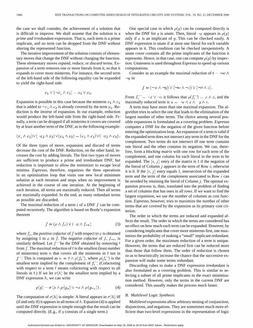
1466 IEEE TRANSACTIONS ON COMPUTER AIDED DESIGN OF INTEGRATED CIRCUITS AND SYSTEMS, VOL. 19, NO. 12, DECEMBER 2000
the case we shall consider, the achievement of a solution thatis difficult to improve. We shall assume that the solution is aprime and irredundantexpression. That is, each term is a primeimplicant, and no term can be dropped from the DNF withoutaltering the represented function.
The iterative improvement of the solution consists of elemen-tary moves that change the DNF without changing the function.These elementary movesexpand, reduce, or discardterms. Ex-pansion of a term removes one or more literals from it, so that itexpands to cover more minterms. For instance, the second termof the left-hand side of the following equality can be expandedto yield the right-hand side:
Expansion is possible in this case because the mintermthat is added to is already covered by the term. Re-duction is the inverse of expansion. In our example, reductionwould produce the left-hand side from the right-hand side. Fi-nally, a term can be dropped if all minterms it covers are coveredby at least another term of the DNF, as in the following example:
Of the three types of move, expansion and discard of termsdecrease the cost of the DNF. Reduction, on the other hand, in-creases the cost by adding literals. The first two types of movesare sufficient to produce a prime and irredundant DNF, butreduction is important to allow the minimizer to escape localminima. Espresso, therefore, organizes the three operationsin an optimization loop that visits one new local minimumsolution at each iteration and stops when no improvement isachieved in the course of one iteration. At the beginning ofeach iteration, all terms are maximally reduced. Then all termsare maximally expanded. In the end, as many redundant termsas possible are discarded.
The maximal reduction of a termof a DNF can be com-puted recursively. The algorithm is based on Boole’s expansiontheorem
(3)
where , thepositive cofactorof with respect to is obtainedby assigning 1 to in . The negative cofactorof , , issimilarly defined. Let be the DNF obtained by removingfrom . The maximal reduction ofis the smallest (least numberof minterms) term that covers all the minterms innot in
. This is computed as , where is thesmallest term implied by the complement of . (Cofactoringwith respect to a term means cofactoring with respect to allliterals in .) If we let be the smallest term implied by aDNF expression , we can write
(4)
The computation of is simple: A literal appears in iff(if and only if) it appears in all terms of. Equation (4) is applieduntil the DNF expression is simple enough that the result can becomputed directly. (E.g., if consists of a single term.)
One special case in which can be computed directly iswhen the DNF for is unate. Then, literal appears inonly if is an implicant of . This can be checked easily. ADNF expression is unate if at most one literal for each variableappears in it. This condition can be checked inexpensively. Aunate cover contains all the prime implicants of the function itrepresents. Hence, in that case, one can computeby inspec-tion. Unateness is used throughoutEspressoto speed up variouscomputations.
Consider as an example the maximal reduction ofin
From it follows that , and themaximally reduced term is .
A term may have more than one maximal expansion. The al-gorithm tries to select the one that leads to the elimination of thelargest number of other terms. The choice among several pos-sible expansions is formulated as a covering problem.Espressocomputes a DNF for the negation of the given function beforeentering the optimization loop. An expansion of a term is valid ifthe expanded term does not intersect any term in the DNF for thecomplement. Two terms do not intersect iff one term containsone literal and the other contains its negation. We can, there-fore, form ablocking matrixwith one row for each term of thecomplement, and one column for each literal in the term to beexpanded. The entry of the matrix is 1 if the negation ofthe literal of Column appears in the term of Row; otherwiseit is 0. If the entry equals 1, intersection of the expandedterm and the term of the complement associated to Rowcanbe avoided by retaining the literal of Column. The optimal ex-pansion process is, thus, translated into the problem of findinga set of columns that has ones in all rows. If we want to find thelargest expansion, we use the number of columns as cost func-tion. Espresso, however, tries to maximize the number of otherterms that are covered by the expansion as its primary cost cri-terion.
The order in which the terms are reduced and expanded af-fects the result. The order in which the terms are considered hasno effect on how much each term can be expanded. However, byconsidering implicants that cover more minterms first, one max-imizes the probability of making a “small” implicant redundant.For a given order, the maximum reduction of a term is unique.However, the terms that are reduced first can be reduced morethan those that follow them. The order of reduction is chosenso as to heuristically increase the chance that the successive ex-pansion will make some terms redundant.
Discarding cubes to make a DNF expression irredundant isalso formulated as a covering problem. This is similar to se-lecting a subset of all prime implicants in the exact minimiza-tion method. However, only the terms in the current DNF areconsidered. This usually makes the process much faster.
B. Multilevel Logic Synthesis
Multilevel expressions allow arbitrary nesting of conjunction,disjunctions, and negations. They are sometimes much more ef-ficient than two-level expressions in the representation of logic
Authorized licensed use limited to: UNIVERSITY OF WINDSOR. Downloaded on May 19, 2009 at 18:19 from IEEE Xplore. Restrictions apply.
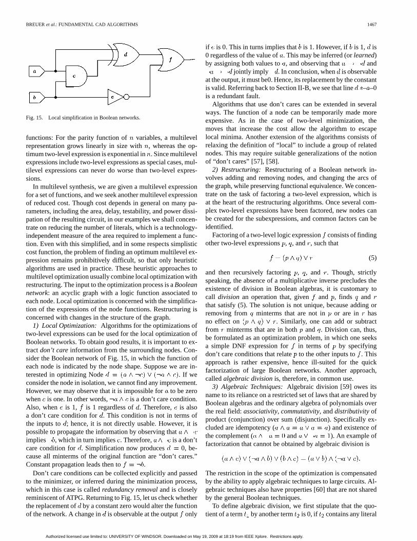
BREUERet al.: FUNDAMENTAL CAD ALGORITHMS 1467
Fig. 15. Local simplification in Boolean networks.
functions: For the parity function of variables, a multilevelrepresentation grows linearly in size with, whereas the op-timum two-level expression is exponential in. Since multilevelexpressions include two-level expressions as special cases, mul-tilevel expressions can never do worse than two-level expres-sions.
In multilevel synthesis, we are given a multilevel expressionfor a set of functions, and we seek another multilevel expressionof reduced cost. Though cost depends in general on many pa-rameters, including the area, delay, testability, and power dissi-pation of the resulting circuit, in our examples we shall concen-trate on reducing the number of literals, which is a technology-independent measure of the area required to implement a func-tion. Even with this simplified, and in some respects simplisticcost function, the problem of finding an optimum multilevel ex-pression remains prohibitively difficult, so that only heuristicalgorithms are used in practice. These heuristic approaches tomultilevel optimization usually combine local optimization withrestructuring. The input to the optimization process is aBooleannetwork: an acyclic graph with a logic function associated toeach node. Local optimization is concerned with the simplifica-tion of the expressions of the node functions. Restructuring isconcerned with changes in the structure of the graph.
1) Local Optimization: Algorithms for the optimizations oftwo-level expressions can be used for the local optimization ofBoolean networks. To obtain good results, it is important to ex-tractdon’t careinformation from the surrounding nodes. Con-sider the Boolean network of Fig. 15, in which the function ofeach node is indicated by the node shape. Suppose we are in-terested in optimizing Node . If weconsider the node in isolation, we cannot find any improvement.However, we may observe that it is impossible forto be zerowhen is one. In other words, is a don’t care condition.Also, when is 1, is 1 regardless of . Therefore, is alsoa don’t care condition for . This condition is not in terms ofthe inputs to ; hence, it is not directly usable. However, it ispossible to propagate the information by observing thatimplies , which in turn implies . Therefore, is a don’tcare condition for . Simplification now produces 0, be-cause all minterms of the original function are “don’t cares.”Constant propagation leads then to .
Don’t care conditions can be collected explicitly and passedto the minimizer, or inferred during the minimization process,which in this case is calledredundancy removaland is closelyreminiscent of ATPG. Returning to Fig. 15, let us check whetherthe replacement of by a constant zero would alter the functionof the network. A change in is observable at the outputonly
if is 0. This in turns implies that is 1. However, if is 1, is0 regardless of the value of. This may be inferred (orlearned)by assigning both values to, and observing that and
jointly imply . In conclusion, when is observableat the output, it must be0. Hence, its replacement by the constantis valid. Referring back to Section II-B, we see that line– –0is a redundant fault.
Algorithms that use don’t cares can be extended in severalways. The function of a node can be temporarily made moreexpensive. As in the case of two-level minimization, themoves that increase the cost allow the algorithm to escapelocal minima. Another extension of the algorithms consists ofrelaxing the definition of “local” to include a group of relatednodes. This may require suitable generalizations of the notionof “don’t cares” [57], [58].
2) Restructuring: Restructuring of a Boolean network in-volves adding and removing nodes, and changing the arcs ofthe graph, while preserving functional equivalence. We concen-trate on the task of factoring a two-level expression, which isat the heart of the restructuring algorithms. Once several com-plex two-level expressions have been factored, new nodes canbe created for the subexpressions, and common factors can beidentified.
Factoring of a two-level logic expressionconsists of findingother two-level expressions, , and , such that
(5)
and then recursively factoring, , and . Though, strictlyspeaking, the absence of a multiplicative inverse precludes theexistence of division in Boolean algebras, it is customary tocall division an operation that, given and , finds andthat satisfy (5). The solution is not unique, because adding orremoving from minterms that are not in or are in hasno effect on . Similarly, one can add or subtractfrom minterms that are in both and . Division can, thus,be formulated as an optimization problem, in which one seeksa simple DNF expression for in terms of by specifyingdon’t care conditions that relateto the other inputs to . Thisapproach is rather expensive, hence ill-suited for the quickfactorization of large Boolean networks. Another approach,calledalgebraic divisionis, therefore, in common use.
3) Algebraic Techniques:Algebraic division [59] owes itsname to its reliance on a restricted set of laws that are shared byBoolean algebras and the ordinary algebra of polynomials overthe real field:associativity, commutativity, anddistributivity ofproduct (conjunction) over sum (disjunction). Specifically ex-cluded are idempotency ( ) and existence ofthe complement ( and ). An example offactorization that cannot be obtained by algebraic division is
The restriction in the scope of the optimization is compensatedby the ability to apply algebraic techniques to large circuits. Al-gebraic techniques also have properties [60] that are not sharedby the general Boolean techniques.
To define algebraic division, we first stipulate that the quo-tient of a term by another term is 0, if contains any literal
Authorized licensed use limited to: UNIVERSITY OF WINDSOR. Downloaded on May 19, 2009 at 18:19 from IEEE Xplore. Restrictions apply.
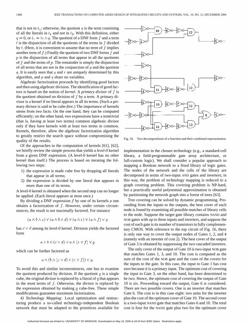
1468 IEEE TRANSACTIONS ON COMPUTER AIDED DESIGN OF INTEGRATED CIRCUITS AND SYSTEMS, VOL. 19, NO. 12, DECEMBER 2000
that is not in ; otherwise, the quotient is the term consistingof all the literals in and not in . With this definition, either
0, or . The quotient of a DNF form and a termis the disjunction of all the quotients of the terms individed
by . (Here, it is convenient to assume that no term ofimpliesanother term of .) Finally the quotient of two DNF forms and
is the disjunction of all terms that appear in all the quotientsof and the terms of. The remainder is simply the disjunctionof all terms that are not in the conjunction ofand the quotient. It is easily seen that and are uniquely determined by this
algorithm, and and share no variables.Algebraic factorization proceeds by identifying good factors
and then using algebraic division. The identification of good fac-tors is based on the notion ofkernel. A primary divisorof isthe quotient obtained on division ofby a term. A primary di-visor is a kernel if no literal appears in all its terms. (Such a pri-mary divisor is said to becube-free.) The importance of kernelsstems from two facts: On the one hand, they can be computedefficiently; on the other hand, two expressions have a nontrivial(that is, having at least two terms) common algebraic divisoronly if they have kernels with at least two terms in common.Kernels, therefore, allow the algebraic factorization algorithmto greatly restrict the search space without compromising thequality of the results.
Of the approaches to the computation of kernels [61], [62],we briefly review the simple process that yields alevel-0kernelfrom a given DNF expression. (A level-0 kernel has no otherkernel than itself.) The process is based on iterating the fol-lowing two steps:
1) the expression is made cube free by dropping all literalsthat appear in all terms;
2) the expression is divided by one literal that appears inmore than one of its terms.
A level-0 kernel is obtained when the second step can no longerbe applied. (Each literal appears at most once.)
By dividing a DNF expression by one of its kernels oneobtains a factorization of . However, under certain circum-stances, the result is not maximally factored. For instance
has among its level-0 kernel. Division yields the factoredform
which can be further factored as
To avoid this and similar inconveniences, one has to examinethe quotient produced by division. If the quotientis a singlecube, the original divisor is replaced by a literal ofthat appearsin the most terms of . Otherwise, the divisor is replaced bythe expression obtained by makingcube-free. These simplemodifications guarantee maximum factorization.
4) Technology Mapping:Local optimization and restruc-turing produce a so-called technology-independent Booleannetwork that must be adapted to the primitives available for
Fig. 16. Two decompositions of a function and their combined representation.
implementation in the chosen technology (e.g., a standard-celllibrary, a field-programmable gate array architecture, orfull-custom logic). We shall consider a popular approach tomapping a Boolean network to a fixed library of logic gates.The nodes of the network and the cells of the library aredecomposed in terms of two-inputAND gates and inverters; inthis way, the problem of technology mapping is reduced to agraph covering problem. This covering problem is NP-hard,but a practically useful polynomial approximation is obtainedby partitioning the network graph into a forest of trees [63].
Tree covering can be solved by dynamic programming. Pro-ceeding from the inputs to the outputs, the best cover of eachnode is found by examining all possible matches of library cellsto the node. Suppose the target gate library containsNAND andNOR gates with up to three inputs and inverters, and suppose thecost of each gate is its number of transistors in fully complemen-tary CMOS. With reference to the top circuit of Fig. 16, thereis only one way to cover the output nodes of Gates 1, 2, and 4(namely with an inverter of cost 2). The best cover of the outputof Gate 3 is obtained by suppressing the two cascaded inverters.
The only cover of the output of Gate 10 is two-inputNORgatethat matches Gates 1, 3, and 10. The cost is computed as thesum of the cost of theNOR gate and the costs of the covers forthe inputs to the gate. In this case, the input to Gate 1 has costzero because it is a primary input. The optimum cost of coveringthe input to Gate 3, on the other hand, has been determined tobe two. Hence, the optimum cost of covering the output of Gate10 is six. Proceeding toward the output, Gate 6 is considered.There are two possible covers. One is an inverter that matchesGate 6. The cost is in this case eight: two units for the inverterplus the cost of the optimum cover of Gate 10. The second coveris a two-inputNAND gate that matches Gates 6 and 10. The totalcost is four for theNAND gate plus two for the optimum cover
Authorized licensed use limited to: UNIVERSITY OF WINDSOR. Downloaded on May 19, 2009 at 18:19 from IEEE Xplore. Restrictions apply.
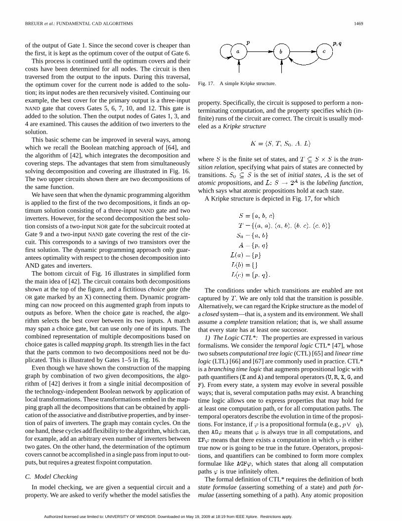
BREUERet al.: FUNDAMENTAL CAD ALGORITHMS 1469
of the output of Gate 1. Since the second cover is cheaper thanthe first, it is kept as the optimum cover of the output of Gate 6.
This process is continued until the optimum covers and theircosts have been determined for all nodes. The circuit is thentraversed from the output to the inputs. During this traversal,the optimum cover for the current node is added to the solu-tion; its input nodes are then recursively visited. Continuing ourexample, the best cover for the primary output is a three-inputNAND gate that covers Gates 5, 6, 7, 10, and 12. This gate isadded to the solution. Then the output nodes of Gates 1, 3, and4 are examined. This causes the addition of two inverters to thesolution.
This basic scheme can be improved in several ways, amongwhich we recall the Boolean matching approach of [64], andthe algorithm of [42], which integrates the decomposition andcovering steps. The advantages that stem from simultaneouslysolving decomposition and covering are illustrated in Fig. 16.The two upper circuits shown there are two decompositions ofthe same function.
We have seen that when the dynamic programming algorithmis applied to the first of the two decompositions, it finds an op-timum solution consisting of a three-inputNAND gate and twoinverters. However, for the second decomposition the best solu-tion consists of a two-inputNOR gate for the subcircuit rooted atGate 9 and a two-inputNAND gate covering the rest of the cir-cuit. This corresponds to a savings of two transistors over thefirst solution. The dynamic programming approach only guar-antees optimality with respect to the chosen decomposition intoAND gates and inverters.
The bottom circuit of Fig. 16 illustrates in simplified formthe main idea of [42]. The circuit contains both decompositionsshown at the top of the figure, and a fictitiouschoice gate(theOR gate marked by an X) connecting them. Dynamic program-ming can now proceed on this augmented graph from inputs tooutputs as before. When the choice gate is reached, the algo-rithm selects the best cover between its two inputs. A matchmay span a choice gate, but can use only one of its inputs. Thecombined representation of multiple decompositions based onchoice gates is calledmapping graph. Its strength lies in the factthat the parts common to two decompositions need not be du-plicated. This is illustrated by Gates 1–5 in Fig. 16.
Even though we have shown the construction of the mappinggraph by combination of two given decompositions, the algo-rithm of [42] derives it from a single initial decomposition ofthe technology-independent Boolean network by application oflocal transformations. These transformations embed in the map-ping graph all the decompositions that can be obtained by appli-cation of the associative and distributive properties, and by inser-tion of pairs of inverters. The graph may contain cycles. On theone hand, these cycles add flexibility to the algorithm, which can,for example, add an arbitrary even number of inverters betweentwo gates. On the other hand, the determination of the optimumcovers cannot be accomplished in a single pass from input to out-puts, but requires a greatest fixpoint computation.
C. Model Checking
In model checking, we are given a sequential circuit and aproperty. We are asked to verify whether the model satisfies the
Fig. 17. A simple Kripke structure.
property. Specifically, the circuit is supposed to perform a non-terminating computation, and the property specifies which (in-finite) runs of the circuit are correct. The circuit is usually mod-eled as aKripke structure
where is the finite set of states, and is thetran-sition relation, specifying what pairs of states are connected bytransitions. is the set ofinitial states, is the set ofatomic propositions, and is the labeling function,which says what atomic propositions hold at each state.
A Kripke structure is depicted in Fig. 17, for which
The conditions under which transitions are enabled are notcaptured by . We are only told that the transition is possible.Alternatively, we can regard the Kripke structure as the model ofaclosedsystem—that is, a system and its environment. We shallassume acompletetransition relation; that is, we shall assumethat every state has at least one successor.
1) The Logic CTL*: The properties are expressed in variousformalisms. We consider thetemporal logicCTL* [47], whosetwo subsetscomputational tree logic(CTL) [65] andlinear timelogic (LTL) [66] and [67] are commonly used in practice. CTL*is abranching time logicthat augments propositional logic withpath quantifiers ( and ) and temporal operators (, , , , and). From every state, a system may evolve in several possible
ways; that is, several computation paths may exist. A branchingtime logic allows one to express properties that may hold forat least one computation path, or for all computation paths. Thetemporal operators describe the evolution in time of the proposi-tions. For instance, if is a propositional formula (e.g., ),then means that is always true in all computations, and
means that there exists a computation in whichis eithertrue now or is going to be true in the future. Operators, proposi-tions, and quantifiers can be combined to form more complexformulae like , which states that along all computationpaths is true infinitely often.
The formal definition of CTL* requires the definition of bothstate formulae(asserting something of a state) andpath for-mulae(asserting something of a path). Any atomic proposition
Authorized licensed use limited to: UNIVERSITY OF WINDSOR. Downloaded on May 19, 2009 at 18:19 from IEEE Xplore. Restrictions apply.
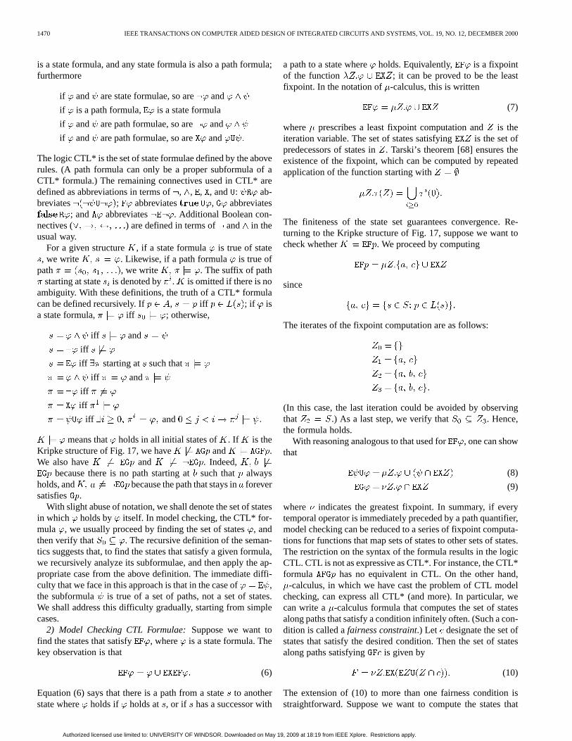
1470 IEEE TRANSACTIONS ON COMPUTER AIDED DESIGN OF INTEGRATED CIRCUITS AND SYSTEMS, VOL. 19, NO. 12, DECEMBER 2000
is a state formula, and any state formula is also a path formula;furthermore
if and are state formulae, so are and
if is a path formula, is a state formula
if and are path formulae, so are and
if and are path formulae, so are and
The logic CTL* is the set of state formulae defined by the aboverules. (A path formula can only be a proper subformula of aCTL* formula.) The remaining connectives used in CTL* aredefined as abbreviations in terms of, , , , and : ab-breviates ; abbreviates , abbreviates
; and abbreviates . Additional Boolean con-nectives ( ) are defined in terms of and in theusual way.
For a given structure , if a state formula is true of state, we write . Likewise, if a path formula is true of
path , we write . The suffix of pathstarting at state is denoted by . is omitted if there is no
ambiguity. With these definitions, the truth of a CTL* formulacan be defined recursively. If , iff ; if isa state formula, iff ; otherwise,
iff and
iff
iff starting at such that
iff and
iff
iff
iff and
means that holds in all initial states of . If is theKripke structure of Fig. 17, we have and .We also have and . Indeed,
because there is no path starting atsuch that alwaysholds, and because the path that stays inforeversatisfies .
With slight abuse of notation, we shall denote the set of statesin which holds by itself. In model checking, the CTL* for-mula , we usually proceed by finding the set of states, andthen verify that . The recursive definition of the seman-tics suggests that, to find the states that satisfy a given formula,we recursively analyze its subformulae, and then apply the ap-propriate case from the above definition. The immediate diffi-culty that we face in this approach is that in the case of ,the subformula is true of a set of paths, not a set of states.We shall address this difficulty gradually, starting from simplecases.
2) Model Checking CTL Formulae:Suppose we want tofind the states that satisfy , where is a state formula. Thekey observation is that
(6)
Equation (6) says that there is a path from a stateto anotherstate where holds if holds at , or if has a successor with
a path to a state whereholds. Equivalently, is a fixpointof the function ; it can be proved to be the leastfixpoint. In the notation of -calculus, this is written
(7)
where prescribes a least fixpoint computation andis theiteration variable. The set of states satisfying is the set ofpredecessors of states in. Tarski’s theorem [68] ensures theexistence of the fixpoint, which can be computed by repeatedapplication of the function starting with
The finiteness of the state set guarantees convergence. Re-turning to the Kripke structure of Fig. 17, suppose we want tocheck whether . We proceed by computing
since
The iterates of the fixpoint computation are as follows:
(In this case, the last iteration could be avoided by observingthat .) As a last step, we verify that . Hence,the formula holds.
With reasoning analogous to that used for , one can showthat
(8)
(9)
where indicates the greatest fixpoint. In summary, if everytemporal operator is immediately preceded by a path quantifier,model checking can be reduced to a series of fixpoint computa-tions for functions that map sets of states to other sets of states.The restriction on the syntax of the formula results in the logicCTL. CTL is not as expressive as CTL*. For instance, the CTL*formula has no equivalent in CTL. On the other hand,
-calculus, in which we have cast the problem of CTL modelchecking, can express all CTL* (and more). In particular, wecan write a -calculus formula that computes the set of statesalong paths that satisfy a condition infinitely often. (Such a con-dition is called afairness constraint.) Let designate the set ofstates that satisfy the desired condition. Then the set of statesalong paths satisfying is given by
(10)
The extension of (10) to more than one fairness condition isstraightforward. Suppose we want to compute the states that
Authorized licensed use limited to: UNIVERSITY OF WINDSOR. Downloaded on May 19, 2009 at 18:19 from IEEE Xplore. Restrictions apply.
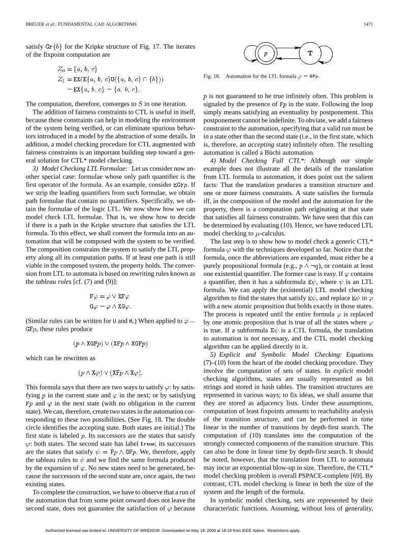
BREUERet al.: FUNDAMENTAL CAD ALGORITHMS 1471
satisfy for the Kripke structure of Fig. 17. The iteratesof the fixpoint computation are
The computation, therefore, converges toin one iteration.The addition of fairness constraints to CTL is useful in itself,
because these constraints can help in modeling the environmentof the system being verified, or can eliminate spurious behav-iors introduced in a model by the abstraction of some details. Inaddition, a model checking procedure for CTL augmented withfairness constraints is an important building step toward a gen-eral solution for CTL* model checking.
3) Model Checking LTL Formulae:Let us consider now an-other special case: formulae whose only path quantifier is thefirst operator of the formula. As an example, consider . Ifwe strip the leading quantifiers from such formulae, we obtainpath formulae that contain no quantifiers. Specifically, we ob-tain the formulae of the logic LTL. We now show how we canmodel check LTL formulae. That is, we show how to decideif there is a path in the Kripke structure that satisfies the LTLformula. To this effect, we shall convert the formula into an au-tomation that will be composed with the system to be verified.The composition constrains the system to satisfy the LTL prop-erty along all its computation paths. If at least one path is stillviable in the composed system, the property holds. The conver-sion from LTL to automata is based on rewriting rules known asthe tableau rules[cf. (7) and (9)]:
(Similar rules can be written for and .) When applied to, these rules produce
which can be rewritten as
This formula says that there are two ways to satisfy: by satis-fying in the current state and in the next; or by satisfying
and in the next state (with no obligation in the currentstate). We can, therefore, create two states in the automation cor-responding to these two possibilities. (See Fig. 18. The doublecircle identifies the accepting state. Both states are initial.) Thefirst state is labeled. Its successors are the states that satisfy
: both states. The second state has label ; its successorsare the states that satisfy . We, therefore, applythe tableau rules to and we find the same formula producedby the expansion of . No new states need to be generated, be-cause the successors of the second state are, once again, the twoexisting states.
To complete the construction, we have to observe that a run ofthe automation that from some point onward does not leave thesecond state, does not guarantee the satisfaction ofbecause
Fig. 18. Automation for the LTL formula' = GFp.
is not guaranteed to be true infinitely often. This problem issignaled by the presence of in the state. Following the loopsimply means satisfying an eventuality by postponement. Thispostponement cannot be indefinite. To obviate, we add a fairnessconstraint to the automation, specifying that a valid run must bein a state other than the second state (i.e., in the first state, whichis, therefore, anacceptingstate) infinitely often. The resultingautomation is called a Büchi automation.
4) Model Checking Full CTL*:Although our simpleexample does not illustrate all the details of the translationfrom LTL formula to automation, it does point out the salientfacts: That the translation produces a transition structure andone or more fairness constraints. A state satisfies the formulaiff, in the composition of the model and the automation for theproperty, there is a computation path originating at that statethat satisfies all fairness constraints. We have seen that this canbe determined by evaluating (10). Hence, we have reduced LTLmodel checking to -calculus.
The last step is to show how to model check a generic CTL*formula with the techniques developed so far. Notice that theformula, once the abbreviations are expanded, must either be apurely propositional formula (e.g., ), or contain at leastone existential quantifier. The former case is easy. Ifcontainsa quantifier, then it has a subformula , where is an LTLformula. We can apply the (existential) LTL model checkingalgorithm to find the states that satisfy , and replace inwith a new atomic proposition that holds exactly in those states.The process is repeated until the entire formulais replacedby one atomic proposition that is true of all the states whereis true. If a subformula is a CTL formula, the translationto automation is not necessary, and the CTL model checkingalgorithm can be applied directly to it.
5) Explicit and Symbolic Model Checking:Equations(7)–(10) form the heart of the model checking procedure. Theyinvolve the computation of sets of states. Inexplicit modelchecking algorithms, states are usually represented as bitstrings and stored in hash tables. The transition structures arerepresented in various ways; to fix ideas, we shall assume thatthey are stored as adjacency lists. Under these assumptions,computation of least fixpoints amounts to reachability analysisof the transition structure, and can be performed in timelinear in the number of transitions by depth-first search. Thecomputation of (10) translates into the computation of thestrongly connected components of the transition structure. Thiscan also be done in linear time by depth-first search. It shouldbe noted, however, that the translation from LTL to automatamay incur an exponential blow-up in size. Therefore, the CTL*model checking problem is overall PSPACE-complete [69]. Bycontrast, CTL model checking is linear in both the size of thesystem and the length of the formula.
In symbolic model checking, sets are represented by theircharacteristic functions. Assuming, without loss of generality,
Authorized licensed use limited to: UNIVERSITY OF WINDSOR. Downloaded on May 19, 2009 at 18:19 from IEEE Xplore. Restrictions apply.
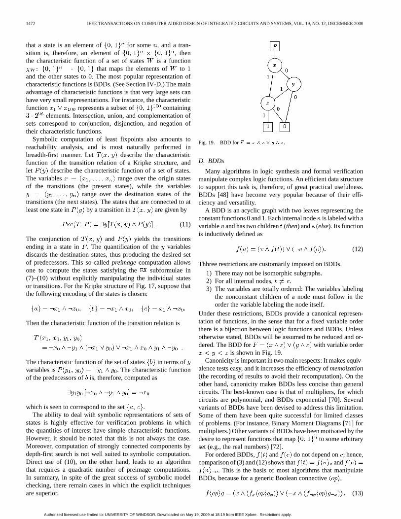
1472 IEEE TRANSACTIONS ON COMPUTER AIDED DESIGN OF INTEGRATED CIRCUITS AND SYSTEMS, VOL. 19, NO. 12, DECEMBER 2000
that a state is an element of for some , and a tran-sition is, therefore, an element of , thenthe characteristic function of a set of states is a function
that maps the elements of to 1and the other states to 0. The most popular representation ofcharacteristic functions is BDDs. (See Section IV-D.) The mainadvantage of characteristic functions is that very large sets canhave very small representations. For instance, the characteristicfunction represents a subset of containing
elements. Intersection, union, and complementation ofsets correspond to conjunction, disjunction, and negation oftheir characteristic functions.
Symbolic computation of least fixpoints also amounts toreachability analysis, and is most naturally performed inbreadth-first manner. Let describe the characteristicfunction of the transition relation of a Kripke structure, andlet describe the characteristic function of a set of states.The variables range over the origin statesof the transitions (the present states), while the variables
range over the destination states of thetransitions (the next states). The states that are connected to atleast one state in by a transition in are given by
(11)
The conjunction of and yields the transitionsending in a state in . The quantification of the variablesdiscards the destination states, thus producing the desired setof predecessors. This so-calledpreimagecomputation allowsone to compute the states satisfying the subformulae in(7)–(10) without explicitly manipulating the individual statesor transitions. For the Kripke structure of Fig. 17, suppose thatthe following encoding of the states is chosen:
Then the characteristic function of the transition relation is
The characteristic function of the set of states in terms ofvariables is . The characteristic functionof the predecessors ofis, therefore, computed as
which is seen to correspond to the set .The ability to deal with symbolic representations of sets of
states is highly effective for verification problems in whichthe quantities of interest have simple characteristic functions.However, it should be noted that this is not always the case.Moreover, computation of strongly connected components bydepth-first search is not well suited to symbolic computation.Direct use of (10), on the other hand, leads to an algorithmthat requires a quadratic number of preimage computations.In summary, in spite of the great success of symbolic modelchecking, there remain cases in which the explicit techniquesare superior.
Fig. 19. BDD forF = x ^ z _ y ^ z.
D. BDDs
Many algorithms in logic synthesis and formal verificationmanipulate complex logic functions. An efficient data structureto support this task is, therefore, of great practical usefulness.BDDs [48] have become very popular because of their effi-ciency and versatility.
A BDD is an acyclic graph with two leaves representing theconstant functions 0 and 1. Each internal nodeis labeled with avariable and has two children(then) and (else). Its functionis inductively defined as
(12)
Thhree restrictions are customarily imposed on BDDs.
1) There may not be isomorphic subgraphs.2) For all internal nodes, .3) The variables are totally ordered: The variables labeling
the nonconstant children of a node must follow in theorder the variable labeling the node itself.
Under these restrictions, BDDs provide a canonical represen-tation of functions, in the sense that for a fixed variable orderthere is a bijection between logic functions and BDDs. Unlessotherwise stated, BDDs will be assumed to be reduced and or-dered. The BDD for with variable order
is shown in Fig. 19.Canonicity is important in two main respects: It makes equiv-
alence tests easy, and it increases the efficiency ofmemoization(the recording of results to avoid their recomputation). On theother hand, canonicity makes BDDs less concise than generalcircuits. The best-known case is that of multipliers, for whichcircuits are polynomial, and BDDs exponential [70]. Severalvariants of BDDs have been devised to address this limitation.Some of them have been quite successful for limited classesof problems. (For instance, Binary Moment Diagrams [71] formultipliers.) Other variants of BDDs have been motivated by thedesire to represent functions that map to some arbitraryset (e.g., the real numbers) [72].
For ordered BDDs, and do not depend on; hence,comparison of (3) and (12) shows that and
. This is the basis of most algorithms that manipulateBDDs, because for a generic Boolean connective,
(13)
Authorized licensed use limited to: UNIVERSITY OF WINDSOR. Downloaded on May 19, 2009 at 18:19 from IEEE Xplore. Restrictions apply.
BREUERet al.: FUNDAMENTAL CAD ALGORITHMS 1473
Equation (13) is applied with chosen as the first variable inthe order that appears in eitheror . This guarantees that thecofactors can be computed easily: Ifdoes not appear in, then
; otherwise, is thethenchild of , and istheelsechild. Likewise, for . The terminal cases of the recur-sion depend on the specific operator. For instance, when com-puting the conjunction of two BDDs, the result is immediatelyknown if either operand is constant, or if the two operands areidentical or complementary. All these conditions can be checkedin constant time if the right provisions are made in the data struc-tures [73].
Two tables are used by most BDD algorithms: Theuniquetable allows the algorithm to access all nodes using the triple
as key. The unique table is consulted before creating anew node. If a node with the desired key is already in existence,it is re-utilized. This approach guarantees that equivalent func-tions will share the same BDD, rather than having isomorphicBDDs; therefore, equivalence checks are performed in constanttime.
Thecomputed tablestores recent operations and their results.Without the computed table, most operations on BDDs wouldtake time exponential in the number of variables. With a losslesscomputed table (one that records the results of all previous com-putations) the time for most common operations is polynomialin the size of the operands. The details of the implementationof the unique and computed tables dramatically affect the per-formance of BDD manipulation algorithms, and have been thesubject of careful study [74].
The order of variables may have a large impact on the sizeof the BDD for a given function. For adders, for instance, theoptimal orders give BDDs of linear size, while bad orders lead toexponential BDDs. The optimal ordering problem for BDDs ishard [75]. Hence, various methods have been proposed to eitherderive a variable order from inspection of the circuit for whichBDDs must be built, or by dynamically computing a good orderwhile the BDDs are built [76].
An exhaustive list of applications of BDDs to problems inCAD is too long to be attempted here. Besides symbolic modelchecking, which was examined in Section IV-C-5, BDD-basedalgorithms have been proposed for most synthesis tasks,including two-level minimization, local optimization, factor-ization, and technology mapping. In spite of their undeniablesuccess, BDDs are not a panacea; their use is most profitablewhen the algorithms capitalize on their strengths [77], andavoid their weaknesses by combining BDDs with other rep-resentations [44], [45], [78]; for instance with satisfiabilitysolvers for CNF expressions.
V. CONCLUSION
Even within generous space limits we could only afford to ad-dress very few of the algorithms currently in use for test, phys-ical design, synthesis, and verification. The following trends canbe identified:
• Although tremendous progress has been made, effectiveand efficient new algorithms are still needed in all aspectsof VLSI CAD.
• Full scan is becoming a de facto standard for testing anddiagnosis for sequential circuits.
• BIST is commonly used for array structures and its usewill continue to expand at a rapid rate.
• New fault modes will be addressed that deal with cross-coupling electrical phenomena, such as crosstalk, signalintegrity, and process variation.
• Manufacturing test techniques will be employed to agreater extent to design validation as the use of functionaltests become less useful.
• Congestion minimization and interaction of conges-tion and timing in placement is a fundamental andunder-studied problem.
• Integration of logic and physical design will be a dom-inant theme in logic synthesis research. The current ap-proaches were not designed to deal with the challenges ofdeep submicron processes. This often leads to decrease inproductivity when designers have to go through several it-erations to solve timing, or signal immunity problems. Thesolutions that will be proposed will include a tighter inte-gration of layout and logic optimization, and the adoptionof more controlled design styles (both logic and physical).
• Reconfigurable computers are likely to fill the gap be-tween general-purpose programmable components andASICs. New logic design problems will emerge that willdemand new algorithms for their efficient solutions.
• Formal verification will increasingly rely on abstrac-tion techniques and compositional approaches likeassume/guarantee reasoning. Semi-formal approaches,that is, approaches that help increase the confidence in thecorrectness of a design by augmenting simulation-basedverification with formal techniques, will become impor-tant.
• From the point of view of the CAD developer, the integra-tion of various engines into powerful tools will becomemore prevalent.
REFERENCES
[1] M. Abramovici, M. A. Breuer, and A. D. Friedman,Digital SystemsTesting and Testable Design. Piscataway, NJ: IEEE Press, 1990.
[2] J. P. Roth, “Diagnosis and automatic failures: A calculus and a method,”IBM J. Res. Develop., vol. 1, no. 4, pp. 278–291, July 1966.
[3] P. Goel, “An implicit enumeration algorithm to generate tests for com-binational logic circuits,”IEEE Trans. Comput., vol. C-30, no. 3, pp.215–222, Ma. 1981.
[4] H. Fujiwara and T. Shimono, “On the acceleration of test generationalgorithms,”IEEE Trans. Compute., vol. C-32, no. 12, pp. 1137–1144,Dec. 1983.
[5] S. Seshu, “On an improved diagnosis program,”IEEE Trans. Electron.Comput., vol. EC-12, pp. 76–79, Feb. 1965.
[6] J. A. Waicukauski, E. B. Eichelberger, D. O. Forlenza, E. Lindbloom,and J. McCarthy, “Fault simulation for structured VLSI,”VLSI Syst. De-sign, vol. 6, no. 12, pp. 20–32, Dec. 1985.
[7] D. B. Armstrong, “A deductive method for simulating faults in logiccircuits,” IEEE Trans. Comput., vol. C-21, pp. 464–471, May 1972.
[8] E. G. Ulrich and T. G. Baker, “Concurrent simulation of nearly identicaldigital networks,”IEEE Trans. Comput., vol. 7, pp. 39–44, Apr. 1974.
[9] M. Abramovici, P. R. Menon, and D. T. Miller, “Critical path tracing:An alternative to fault simulation,”IEEE Design Test Comput., vol. 1,no. 1, pp. 83–93, Feb. 1984.
[10] M. Abramovici and M. A. Breuer, “Multiple fault diagnosis in combi-national circuits based on effect-cause analysis,”IEEE Trans. Comput.,vol. C-29, no. 6, pp. 451–460, June 1980.
Authorized licensed use limited to: UNIVERSITY OF WINDSOR. Downloaded on May 19, 2009 at 18:19 from IEEE Xplore. Restrictions apply.
1474 IEEE TRANSACTIONS ON COMPUTER AIDED DESIGN OF INTEGRATED CIRCUITS AND SYSTEMS, VOL. 19, NO. 12, DECEMBER 2000
[11] , “Fault diagnosis in synchronous sequential circuits based on aneffect-cause analysis,”IEEE Trans. Comput., vol. C-31, no. 12, pp.1162–1172, Dec. 1982.
[12] M. Abromovici, “Fault diagnosis in digital circuits based an effect-causeanalysis, Ph.D. dissertation,” Univ. Southern California and USCEE,Tech. Rep. 508, 1980.
[13] B. W. Kernighan and S. Lin, “An efficient heuristic procedure for parti-tioning graphs,”Bell Syst. Tech. J., vol. 49, pp. 291–307, Feb. 1970.
[14] C. M. Fiduccia and R. M. Mattheyes, “A linear time heuristic for im-proving network partitions,” inProc. IEEE-ACM Design AutomationConf., 1982, pp. 175–181.
[15] B. Krishnamurthy, “An improved min-cut algorithm for partitioningVLSI networks,” IEEE Trans. Comput., vol. C-33, pp. 438–446, May1984.
[16] J. Cong and M. L. Smith, “A parallel bottom-up clustering algorithmwith applications to circuit partitioning in VLSI design,” inProc.IEEE-ACM Design Automation Conf., 1993, pp. 755–760.
[17] B. Hendrickson and R. Leland, “A multilevel algorithm for partitioninggraphs,” Sandia National Laboratories, Tech. Rep. SAND93-1301,1993.
[18] S. Hauck and G. Boriello, “An evaluation of bipartitioning tech-niques,” presented at the Chapel Hill Conf. Advanced Research inVLSI, 1995.
[19] G. Karypis and V. Kumar, “A fast and highly quality multilevel schemefor partitioning irregular graphs,”SIAM J. Scientific Computing, vol. 20,no. 1, pp. 359–392, 1999.
[20] , “METIS 3.0: Unstructured graph partitioning and sparse matrixordering system,” Department of Computer Science, University of Min-nesota, Tech. Rep. 97-061, 1997.
[21] G. Karypis, R. Aggarwal, V. Kumar, and S. Shekhar, “Multilevel hyper-graph partitioning: Application in VLSI domain,” inProc. IEEE-ACMDesign Automation Conf., 1997, pp. 526–529.
[22] G. Karypis and V. Kumar, “Multilevelk-way hypergraph partitioning,”in Proc. IEEE-ACM Design Automation Conf., 1999, pp. 343–348.
[23] C. Alpert, “The ISPD98 circuit benchmark suite,” inProc. Int. Symp.Physical Design: ACM, Apr. 1998, pp. 18–25.
[24] S. Rao, “Finding near optimal separators in planar graphs,” inProc.Symp. Foundations of Computer Science, 1987, pp. 225–237.
[25] S. Wimer, I. Koren, and I. Cederbaum, “Optimal aspect ratios ofbuilding blocks in VLSI,” IEEE Trans. Computer-Aided Design, vol.8, pp. 139–145, Feb. 1989.
[26] J. P. Cohoon, “Distributed genetic algorithms for the floorplan designproblem,” IEEE Trans. Computer-Aided Design, vol. 10, no. 4, pp.483–492, April 1991.
[27] D. F. Wong, H. W. Leong, and C. L. Liu,Simulated Annealing for VLSIDesign: Kluwer Academic, 1988.
[28] R. M. Kling and P. Banerjee, “Optimization by simulated evolution withapplications to standard cell placement,” inProc. IEEE-ACM DesignAutomation Conf., 1990, pp. 20–25.
[29] M. Rebaudengo and M. S. Reorda, “GALLO: A genetic algorithm forfloorplan area optimization,”IEEE Trans. Computer-Aided Design, vol.15, pp. 943–951, Aug. 1996.
[30] J. M. Kleinhans, G. Sigl, F. M. Johannes, and K. J. Antreich, “GOR-DIAN: VLSI placement by quadratic programming and slicing opti-mization,” IEEE Trans. Computer-Aided Design, vol. 10, p. 365, Mar.1991.
[31] C. Alpert, T. Chan, D. Huang, and A. B. Kahng, “Faster minimizationof linear wirelength for global placement,” inProc. Int. Symp PhysicalDesign: ACM, 1997, pp. 4–11.
[32] T. Lengauer and M. Lugering, “Integer programming formulation ofglobal routing and placement problems,” inAlgorithm Aspects of VLSILayout, M. Sarrafzadeh and D. T. Lee, Eds, Singapore: World Sceintific,1993.
[33] S. Kirkpatrick, C. D. Gelatt Jr., and M. P. Vecchi, “Optimization by sim-ulated annealing,”Science, vol. 220, pp. 671–680, 1983.
[34] G. Sigl, K. Doll, and F. M. Johannes, “Analytical placement: A linear ora quadratic objective function,” inProc. IEEE-ACM Design AutomationConference, 1991, pp. 427–431.
[35] D. Huang and A. B. Kahng, “Partitioning-based standard-cell globalplacement with an exact objective,” inProc. Int. Symp. Physical De-sign, Apr. 1997, pp. 18–25.
[36] H. Eisenmann and F. M. Johannes, “Generic global placement andfloorplanning,” in Proc. IEEE-ACM Design Automation Conf., 1998,pp. 269–274.
[37] R. Nair, “A simple yet effective technique for global wiring,”IEEETrans. Computer-Aided Design, vol. CAD-6, pp. 165–172, Mar.1987.
[38] M. Wang and M. Sarrafzadeh, “Behavior of congestion minimizationduring placement,” inProc. Int. Symp. Physical Design, April 1999, pp.145–150.
[39] C. Y. Lee, “An algorithm for path connection and its application,”IRETrans. Electron. Comput., vol. EC-10, pp. 346–365, 1961.
[40] A. Kahng, J. Cong, and G. Robins, “High-performance clock routingbased on recursive geometric matching,” inProc. IEEE-ACM DesignAutomation Conf.: IEEE/ACM, 1991, pp. 322–327.
[41] J. Cong and C. K. Koh, “Minimum-cost bounded-skew clock routing,”in Proc. IEEE Int. Symp. Circuits and Systems, 1995, pp. 215–218.
[42] E. Lehman, Y. Watanabe, J. Grodstein, and H. Harkness, “Logic decom-position during technology mapping,”IEEE Trans. Computer-Aided De-sign, vol. 16, pp. 813–834, Aug. 1995.
[43] M. Pedram, “Power minimization in IC design: Principles and applica-tions,” ACM Trans. Design Automat. Electron. Syst., vol. 1, no. 1, pp.3–56, 1996.
[44] A. Kuehlmann and F. Krohm, “Equivalence checking using cuts andheaps,” inProc. IEEE-ACM Design Automation Conf., Anaheim, CA,June 1997, pp. 263–268.
[45] J. R. Burch and V. Singhal, “Tight integration of combinational veri-fication methods,” inProc. IEEE International Conf. Computer-AidedDesign, San Jose, CA, Nov. 1998, pp. 570–576.
[46] R. P. Kurshan, “Formal verification in a commercial setting,” inProc.IEEE-ACM Design Automation Conf., Anaheim, CA, June 1997, pp.258–262.
[47] E. A. Emerson and J. Y. Halpern, “‘Sometimes’ and ‘not never’ revis-ited: On branching time versus linear time temporal logic,”J. Assoc.Computing Machinery, vol. 33, no. 1, pp. 151–178, 1986.
[48] R. E. Bryant, “Graph-based algorithms for Boolean function manipula-tion,” IEEE Trans. Comput., vol. C-35, pp. 677–691, Aug. 1986.
[49] K. L. McMillan, Symbolic Model Checking. Boston, MA: KluwerAcademic, 1994.
[50] W. V. Quine, “Two theorems about truth functions,”Boletin de la So-ciedad Matematica Mexicana, vol. 10, pp. 64–70, 1953.
[51] E. J. McCluskey Jr., “Minimization of Boolean functions,”Bell Syst.Tech. J., vol. 35, pp. 1417–1444, Nov. 1956.
[52] J. F. Gimpel, “A method of producing a Boolean function having anarbitrarily prescribed prime implicant table,”IEEE Trans. Electron.Comput., vol. EC-14, pp. 485–488, June 1965.
[53] O. Coudert and J. C. Madre, “Implicit and incremental computation ofprimes and essential primes of Boolean functions,” inProc. IEEE-ACMDesign Automation Conf., Anaheim, CA, June 1992, pp. 36–39.
[54] , “New ideas for solving covering problems,” inProc. IEEE-ACMDesign Automation Conf., San Francisco, CA, June 1995, pp. 641–646.
[55] R. K. Brayton, G. D. Hachtel, C. T. McMullen, and A. Sangiovanni-Vin-centelli, Logic Minimization Algorithms for VLSI Synthesis. Boston,MA: Kluwer Academic, 1984.
[56] R. Rudell and A. Sangiovanni-Vincentelli, “Multiple-valued minimiza-tion for PLA optimization,”IEEE Trans. Computer-Aided Design, vol.CAD-6, pp. 727–750, Sept. 1987.
[57] R. K. Brayton and F. Somenzi, “Boolean relations and the incompletespecification of logic networks,” inVLSI’89, G. Musgrave and U.Lauther, Eds. Amsterdam, The Netherlands: North-Holland, 1989,pp. 231–240.
[58] S. Yamashita, H. Sawada, and N. Nagoya, “A new method to expressfunctional permissibilities for LUT based FPGA’s and its applications,”in Proc. IEEE Int. Conf. Computer-Aided Design, San Jose, CA, Nov.1996, pp. 254–261.
[59] R. K. Brayton and C. McMullen, “The decomposition and factorizationof Boolean expressions,” inProc. IEEE Int. Symp. Circuits and Systems,Rome, Italy, May 1982, pp. 49–54.
[60] G. D. Hachtel, R. M. Jacoby, K. Keutzer, and C. R. Morrison, “On prop-erties of algebraic transformations and the synthesis of multifault-irre-dundant circuits,”IEEE Trans. Computer-Aided Design, vol. 11, no. 3,pp. 313–321, Mar. 1992.
[61] R. K. Brayton, G. D. Hachtel, and A. L. Sangiovanni-Vincentelli, “Mul-tilevel logic synthesis,”Proc. IEEE, vol. 78, pp. 264–300, Feb. 1990.
[62] J. Rajski and J. Vasudevamurthy, “The testability-preserving concurrentdecomposition and factorization of Boolean expressions,”IEEE Trans.Computer-Aided Design, vol. 11, pp. 778–793, June 1993.
[63] K. Keutzer, “DAGON: Technology binding and local optimization byDAG matching,” inProc. IEEE-ACM Design Automation Conf., June1987, pp. 341–347.
[64] F. Mailhot and G. De Micheli, “Technology mapping using Booleanmatching,” inProc. Eur. Conf. Design Automation, Glasgow, U.K., Mar.1990, pp. 180–185.
[65] E. M. Clarke and E. A. Emerson, “Design and synthesis of synchro-nization skeletons using branching time temporal logic,” inProceedingsWorkshop on Logics of Programs, ser. LNCS 131. Berlin, Germany:Springer-Verlag, 1981, pp. 52–71.
Authorized licensed use limited to: UNIVERSITY OF WINDSOR. Downloaded on May 19, 2009 at 18:19 from IEEE Xplore. Restrictions apply.
BREUERet al.: FUNDAMENTAL CAD ALGORITHMS 1475
[66] P. Wolper, M. Y. Vardi, and A. P. Sistla, “Reasoning about infinite com-putation paths,” inProc. 24th IEEE Symp. Foundations of Computer Sci-ence, 1983, pp. 185–194.
[67] O. Lichtenstein and A. Pnueli, “Checking that finite state concurrentprograms satisfy their linear specification,” presented at the 12th AnnualACM Symp. Principles of Programming Languages, New Orleans, Jan.1985.
[68] A. Tarski, “A lattice-theoretic fixpoint theorem and its applications,”Pacific J. Math., vol. 5, pp. 285–309, 1955.
[69] E. A. Emerson and C.-L. Lei, “Efficient model checking in fragmentsof the propositional mu-calculus,” inProc. 1st Annu. Symp. Logic inComputer Science, June 1986, pp. 267–278.
[70] R. E. Bryant, “On the complexity of VLSI implementations and graphrepresentations of Boolean functions with application to integer multi-plication,” IEEE Trans. Comput., vol. 40, no. 2, pp. 205–213, Feb. 1991.
[71] R. Bryant and Y.-A. Chen, “Verification of arithmetic circuits with bi-nary moment diagrams,” inProc. IEEE-ACM Design Automation Conf.,San Francisco, CA, June 1995, pp. 535–541.
[72] Y.-T. Lai and S. Sastry, “Edge-valued binary decision diagrams formulti-level hierarchical verification,” inProc. IEEE-ACM DesignAutomation Conf., Anaheim, CA, June 1992, pp. 608–613.
[73] F. Somenzi, “Binary decision diagrams,” inCalculational System De-sign, M. Broy and R. Steinbrüggen, Eds. Amsterdam, The Nether-lands: IOS, 1999, pp. 303–366.
[74] S. Manne, D. C. Grunwald, and F. Somenzi, “Remembrance of thingspast: Locality and memory in BDDs,” inProc. IEEE-ACM Design Au-tomation Conf., Anaheim, CA, June 1997, pp. 196–201.
[75] D. Sieling, “The nonapproximability of OBDD minimization,” Univ.Dortmund, Tech. Rep. 663, 1998.
[76] R. Rudell, “Dynamic variable ordering for ordered binary decision dia-grams,” inProc. IEEE Int. Conf. Computer-Aided Design, Santa Clara,CA, Nov. 1993, pp. 42–47.
[77] K. Ravi and F. Somenzi, “Hints to accelerate symbolic traversal,” inCorrect Hardware Design and Verification Methods (CHARME’99),ser. LNCS 1703. Berlin, Germany: Springer-Verlag, Sept. 1999, pp.250–264.
[78] A. Biere, A. Cimatti, E. Clarke, and Y. Zhu, “Symbolic model checkingwithout BDDs,” inProc. TACAS’99, Mar. 1999, pp. 193–207.
Melvin A. Breuer (S’58–M’65–SM’73–F’85) received the Ph.D. degree inelectrical engineering from the University of California, Berkeley; is currentlya professor of both Electrical Engineering and Computer Science at theUniversity of Southern California, Los Angeles, California.
He is the Charles Lee Powell Professor of Electrical Engineering and Com-puter Science. He was chairman of the Department of Electrical Engineering-Systems from 1991-1994, and is currently chair once again. His main interestsare in the area of computer-aided design of digital systems, design-for-test andbuilt-in self-test, and VLSI circuits. He was chair of the faculty of the School ofEngineering, USC, for the 1997-98 academic year.
Dr. Breuer is the editor and co-author ofDesign Automation of DigitalSystems: Theory and Techniques(Englewood Cliffs, NJ; Prentice-Hall); editorof Digital Systems Design Automation: Languages, Simulation and Data Base(Los Alamitos, CA: Computer Science Press); co-author ofDiagnosis andReliable Design of Digital Systems(Los Alamitos, CA:Computer SciencePress); co-editor ofComputer Hardware Description Languages and theirApplications (Amsterdam, The Netherland: North-Holland); co-editor andcontributor toKnowledge Based Systems for Test and Diagnosis(Amsterdam,The Netherland: North-Holland); and co-author ofDigital System Testing andTestable Design(Los Alamitos, CA: Computer Science Press, 1990; reprintedPiscataway, NJ: IEEE Press, 1995) . He has published over 200 technicalpapers. He was Editor-in-Chief of theJournal of Design Automation andFault Tolerant Computing. He served on the editorial board of theJournal ofElectronic Testingand was the co-editor of theJournal of Digital Systems.He was the Program Chairman of the Fifth International IFIP Conferenceon Computer Hardware Description Languages and Their Applications.He was co-author of a paper that received an honorable mention award atthe 1997 International Test Conference. He was a Fullbright-Hays scholar(1972); received the 1991 Associates Award for Creativity in Research andScholarship from the University of Southern California, the 1991 USC Schoolof Engineering Award for Exceptional Service, and the IEEE ComputerSociety’s 1993 Taylor L. Booth Education Award. He was the keynote speakerat the Fourth Multimedia Technology and Applications Symposium, 1999, andthe Ninth Asian Test Symposium, 2000.
Majid Sarrafzadeh (M’87–SM’92–F’96) receivedthe B.S., M.S. and Ph.D. degrees in 1982, 1984, and1987 respectively from the University of Illinois atUrbana-Champaign in electrical and computer engi-neering.
He joined Northwestern University as an AssistantProfessor in 1987. Since 2000, he has been a Pro-fessor of Computer Science, University of California,Los Angeles. His research interests lie in the area ofVLSI CAD, design and analysis of algorithms andVLSI architecture. He has collaborated with many in-
dustries in the past ten years including IBM and Motorola and many CAD in-dustries.
Dr. Sarrafzadeh is a Fellow of IEEE for his contribution to “Theory and Prac-tice of VLSI Design.” He received a National Science Foundation (NSF) En-gineering Initiation award, two distinguished paper awards in ICCAD, and thebest paper award for physical design in DAC for his work in the area of Phys-ical Design. He has served on the technical program committee of numerousconferences in the area of Physical Design and CAD, including ICCAD, EDACand ISCAS. He has served as committee chairs of a number of these confer-ences, including International Conference on CAD and International Sympo-sium on Physical Design. He was the general chair of the 1998 InternationalSymposium on Physical Design. He has published approximately 180 papers, isCo-Editor ofAlgorithmic Aspects of VLSI Layout(Singapore: World Scientific,1994), Co-Author ofAn Introduction to Physical Design(New York: McGrawHill, 1996), and the author of an invited chapter in theEncyclopedia of Elec-trical and Electronics Engineeringin the area of VLSI Circuit Layout.
Dr. Sarrafzadeh is on the editorial board of theVLSI Design Journal, Co-Ed-itor-in-Chief of theInternational Journal of High-Speed Electronics, an Asso-ciate Editor ofACM Transactions on Design Automation (TODAES), and anAssociate Editor of IEEE TRANSACTIONS ONCOMPUTER-AIDED DESIGN.
Fabio Somenzi received the Dr. Eng. degree inelectronic engineering from Politecnico di Torino,Torino, Italy, in 1980.
He was with SGS-Thomson Microelectronics from1982 to 1989. Since then, he has been with the De-partment of Electrical and Computer Engineering ofthe University of Colorado, Boulder, where he is cur-rently an Associate Professor. His research interestsinclude synthesis, optimization, simulation, verifica-tion, and testing of logic circuits.
Authorized licensed use limited to: UNIVERSITY OF WINDSOR. Downloaded on May 19, 2009 at 18:19 from IEEE Xplore. Restrictions apply.