from rapid diagnostics to a rapid diagnosis - universiteit...
TRANSCRIPT
i
UMC Utrecht histopathology laboratory
From rapid diagnostics to a rapid diagnosis
A.G. Leeftink 8/20/2014

From rapid diagnostics to a rapid diagnosis UMC Utrecht histopathology laboratory
Master Thesis Industrial Engineering and Management
Author Gréanne Leeftink University of Twente, School of Management and Government
UMC Utrecht, Department of Pathology
Supervisors M.A.M. Verdaasdonk UMC Utrecht, Department of Pathology
Prof.dr.ir. E.W. Hans University of Twente, Centre for Healthcare Operations Improvement and Research
Prof.dr. R.J. Boucherie University of Twente, Centre for Healthcare Operations Improvement and Research
Dr.ir. I.M.H. Vliegen University of Twente, Centre for Healthcare Operations Improvement and Research

UMC Utrecht histopathology laboratory A.G. Leeftink
iv
Management summary Background Since 2011, University Medical Center Utrecht has introduced rapid diagnostic pathways for several types of cancer. This involved a change in current practices of multiple departments, including pathology, where tissue of 22.5 thousand patients is evaluated (i.e. for tumorous cells) in the histopathology laboratory each year.
For the department of Pathology the implementation of these pathways involved a change in the current practices. The regular histopathology processes exist of five main steps: grossing, tissue processing, embedding, sectioning and staining slides, and examination of slides, as shown in Figure 1. The tissue processing step is performed by a large batching machine, where the other steps are executed by technicians. The batching machine takes two to 12 hours to process the tissue, depending on the size of the largest tissue in the batch. Therefore, it is regularly done overnight.
Since the introduction of rapid diagnostic pathways requires same day examination, the tissue processing task is performed during the day, which is an exception to the regular processing standards. Furthermore, rapid diagnostic tissues are prioritized over the regular tissue handling.
Problem statement Currently, demand for rapid diagnostic pathways is still increasing. However, more dedicated resources cannot be offered, since this will reduce the performance of the regular care in terms of throughput times (Vanberkel et al., 2012). Additionally, the workload at the histopathology laboratory is not equally divided over the day. In the morning, when the rapid diagnostics main activities are performed, the workload is experienced as too high. Concluding: By prioritizing the processing of rapid diagnostic tissues, all other tissues are delayed and the workload is increasing. Due to this call for improvement, we aim to integrate the rapid diagnostics and regular tissue processing, such that all tissues are timely examined.
Context analysis The current performance of the histopathology laboratory is measured in terms of throughput time (TPT) and workload. The TPT norms for almost all types of tissue are met, except for the prioritized tissues. However, this is likely due to an authorization delay; the diagnosis was delivered on time.
Figure 2 shows the workload on primary activities in the histopathology laboratory indeed exceeds the amount of workers available in the morning and late afternoon. However, in the afternoon, the workload for primary activities is really low.
Modeling results To get insight in the effect of several interventions on the TPT
Grossing Tissue
processing Embedding
Sectioning & staining
Examination
Figure 1: Regular tissue processing steps in the histopathology laboratory
0
2
4
6
8
10
12
7:3
0
8:2
0
9:1
0
10
:00
10
:50
11
:40
12
:30
13
:20
14
:10
15
:00
15
:50
16
:40
17
:30
FTE # primary
activities
# workers
Figure 2: Load of average amount of primary activities over the day (based on House of Performance (2006)) (22379 patients, 2013, LMS)
From rapid diagnostics to a rapid diagnosis A.G. Leeftink
v
and workload, we propose a Mixed Integer Linear Program (MILP). A MILP is an operations research tool that provides mathematical optimization in which the restrictions and objective are formulated as a linear function. The model is modeled in AIMMS 4.0 and solved with CPLEX 12.3. Due to the high computation time of the model, a three-phase solution approach is proposed, to find a near-optimal solution in reasonable time.
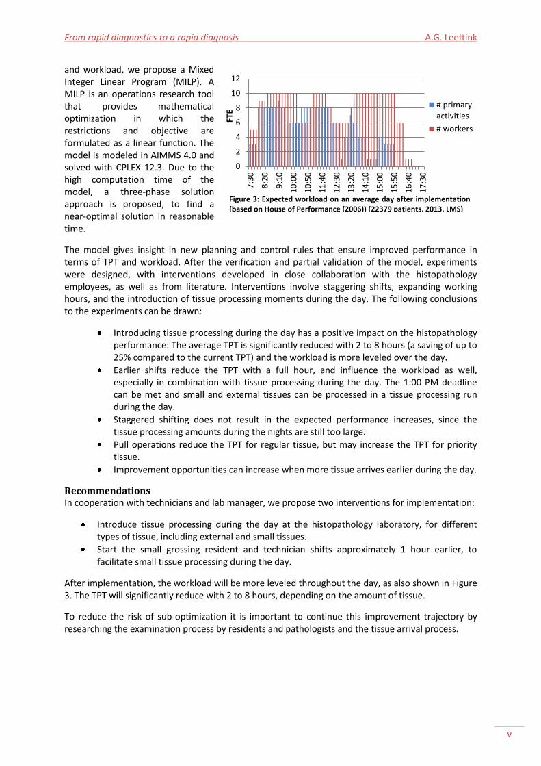
The model gives insight in new planning and control rules that ensure improved performance in terms of TPT and workload. After the verification and partial validation of the model, experiments were designed, with interventions developed in close collaboration with the histopathology employees, as well as from literature. Interventions involve staggering shifts, expanding working hours, and the introduction of tissue processing moments during the day. The following conclusions to the experiments can be drawn:
Introducing tissue processing during the day has a positive impact on the histopathology performance: The average TPT is significantly reduced with 2 to 8 hours (a saving of up to 25% compared to the current TPT) and the workload is more leveled over the day.
Earlier shifts reduce the TPT with a full hour, and influence the workload as well, especially in combination with tissue processing during the day. The 1:00 PM deadline can be met and small and external tissues can be processed in a tissue processing run during the day.
Staggered shifting does not result in the expected performance increases, since the tissue processing amounts during the nights are still too large.
Pull operations reduce the TPT for regular tissue, but may increase the TPT for priority tissue.
Improvement opportunities can increase when more tissue arrives earlier during the day.
Recommendations In cooperation with technicians and lab manager, we propose two interventions for implementation:
Introduce tissue processing during the day at the histopathology laboratory, for different types of tissue, including external and small tissues.
Start the small grossing resident and technician shifts approximately 1 hour earlier, to facilitate small tissue processing during the day.
After implementation, the workload will be more leveled throughout the day, as also shown in Figure 3. The TPT will significantly reduce with 2 to 8 hours, depending on the amount of tissue.
To reduce the risk of sub-optimization it is important to continue this improvement trajectory by researching the examination process by residents and pathologists and the tissue arrival process.
0
2
4
6
8
10
12
7:3
0
8:2
0
9:1
0
10
:00
10
:50
11
:40
12
:30
13
:20
14
:10
15
:00
15
:50
16
:40
17
:30
FTE
# primaryactivities
# workers
Figure 3: Expected workload on an average day after implementation (based on House of Performance (2006)) (22379 patients, 2013, LMS)
UMC Utrecht histopathology laboratory A.G. Leeftink
vi
Management samenvatting (Dutch) Achtergrond Het Universitair Medisch Centrum te Utrecht heeft sinds 2011 sneldiagnostiek-trajecten ingevoerd voor verscheidene typen kanker. Deze implementatie brengt veranderingen teweeg bij verschillende afdelingen, waaronder pathologie, waar menselijk weefsel van 22,5 duizend patiënten per jaar wordt onderzocht op bijvoorbeeld tumorcellen in het histologisch laboratorium.
Het huidige proces in het histologisch laboratorium bestaat uit vijf belangrijke stappen: uitsnijden, doorvoeren, inbedden, snijden en kleuren van coupes, en beoordeling, zoals weergegeven in Figure 1. De doorvoer-stap wordt uitgevoerd door een grote batch-machine. De overige stappen worden uitgevoerd door analisten. De doorvoermachine voert de weefsels in 2 tot 12 uur door, afhankelijk van de grootte van het grootste stuk weefsel in de batch. Daarom wordt normaal gesproken ’s nachts doorgevoerd.
Omdat de invoering van sneldiagnostiek een beoordeling vereist op dezelfde dag, moet sneldiagnostiek-weefsel overdag worden doorgevoerd. Dit is een uitzondering op de reguliere processen. Daarbij heeft de verwerking van sneldiagnostiek-weefsels meer prioriteit dan de verwerking van regulier weefsel.
Probleemstelling De vraag naar sneldiagnostiek-trajecten is nog steeds groeiende. Echter, de prestatie (in doorlooptijd) van de reguliere zorg zal afnemen wanneer daar meer resources voor worden gereserveerd (Vanberkel et al., 2012). Daarbij komt dat de werkdruk in het histologie laboratorium ongelijk verdeeld is over de dag. Vooral ’s morgens, wanneer sneldiagnostiek-taken worden uitgevoerd, wordt een hoge werkdruk ervaren. Concluderend: Door prioritering van sneldiagnostiek-weefsel worden de overige weefsels vertraagd, en loopt de werkdruk op. Daarom beogen wij met dit onderzoek de sneldiagnostiek en reguliere diagnostiek met elkaar te integreren, zodat alle weefsels snel gediagnosticeerd worden.
Context analyse De huidige prestatie van het histologisch laboratorium wordt gemeten in doorlooptijd en werkdruk. De doorlooptijdnormen voor bijna alle weefseltypen worden behaald, behalve die van de geprioriteerde weefsels. Dit wordt waarschijnlijk veroorzaakt door een vertraging in autorisatie; de diagnose was op tijd gesteld.
Figure 2 geeft de werkdruk met betrekking tot de primaire activiteiten in het histologisch laboratorium weer. Hierin wordt laten zien dat de werkdruk inderdaad hoger is dan het aantal beschikbare medewerkers in de morgen en de namiddag. Gedurende de rest van de middag is de werkdruk met betrekking tot de primaire activiteiten erg laag.
Resultaten Een Mixed Integer Linear Program (MILP) is ontwikkeld om inzicht te krijgen in de effecten van verscheidene interventies op de doorlooptijd en werkdruk. Een MILP is een wiskundig optimalisatie programma waarmee restricties en doelen worden geformuleerd als lineaire functies. Het model is gemodelleerd in AIMMS 4.0 en opgelost met CPLEX 12.3. Door de lange rekentijd is een 3-fase methode ontwikkeld die in korte tijd een (bijna-)optimale oplossing kan vinden.
Het model geeft inzicht in nieuwe besturingsregels die ervoor zorgen dat de prestatie verbetert. Na verificatie en gedeeltelijke validatie van het model zijn experimenten ontwikkeld, gebaseerd op interventies. Deze interventies zijn ontwikkeld in nauwe samenwerking met de histologische medewerkers en naar aanleiding van een literatuurstudie. Trapsgewijze werktijden, verlengde
From rapid diagnostics to a rapid diagnosis A.G. Leeftink
vii
werktijden, en de introductie van overdag doorvoeren behoren tot de interventies. Uit de experimenten kan worden geconcludeerd dat:
overdag doorvoeren een positieve impact heeft op de prestatie van het histologisch laboratorium: De doorlooptijd is significant verlaagd met 2 tot 8 uur (dit is een vermindering van ±25% ten opzichte van de huidige doorlooptijd) en de werkdruk is meer verspreid over de dag.
door eerdere starttijden in het laboratorium de doorlooptijd van weefsels een uur wordt verkort. Ook de werkdruk wordt hierdoor verminderd, in het bijzonder in combinatie met overdag doorvoeren. De 1-uurs deadline wordt gemakkelijker gehaald, en ook externe en kleine weefsels kunnen overdag worden doorgevoerd.
trapsgewijze werktijden de verwachte verbetering in prestatie op dit moment niet teweegbrengen door de grote doorvoerhoeveelheden gedurende de nacht.
de histologische prestatie enorm kan verbeteren wanneer weefsel gedurende de dag eerder arriveert bij het laboratorium.
Aanbevelingen In samenwerking met (hoofd-)analisten en de lab manager, bevelen wij twee interventies aan voor implementatie:
Voer meerdere typen weefsel, zoals extern en klein weefsel, overdag door.
Start de werktijden van de ‘kleine-assistent’ en bijbehorende analist één uur eerder, zodat klein weefsel overdag doorgevoerd kan worden.
Na implementatie van deze aanbevelingen, zal de werkdruk meer gespreid zijn over de dag, zoals Figure 3 laat zien. De doorlooptijd zal significant verminderen met 2 tot 8 uur.
Om het risico van sub-optimalisatie te verminderen, is het belangrijk om het ingezette verbetertraject voort te zetten. Onder andere het beoordelingsproces door assistenten en pathologen, en het aankomstproces van weefsels vereisen verder onderzoek.
UMC Utrecht histopathology laboratory A.G. Leeftink
viii
Contents Management summary ........................................................................................................................... iv
Management samenvatting (Dutch) ....................................................................................................... vi
Contents ................................................................................................................................................ viii
Nomenclature ........................................................................................................................................... x
Glossary .................................................................................................................................................... x
Preface ................................................................................................................................................... xiii
Chapter 1 |Project description ................................................................................................................ 1
1.1 |Pathology at UMC Utrecht .......................................................................................................... 1
1.2 |Rapid diagnostics ......................................................................................................................... 1
1.3 |Problem definition ....................................................................................................................... 2
1.4 |Objective and approach............................................................................................................... 3
1.5 |Challenges .................................................................................................................................... 5
Chapter 2 |Context analysis .................................................................................................................... 7
2.1 |Process description ...................................................................................................................... 7
2.2 |Planning and control .................................................................................................................. 12
2.3 |Performance .............................................................................................................................. 15
2.4 |Conclusions ................................................................................................................................ 23
Chapter 3 |Theoretical framework ....................................................................................................... 27
3.1 |Histopathology laboratory optimization ................................................................................... 27
3.2 |Where we work ......................................................................................................................... 27
3.3 |How we work ............................................................................................................................. 28
3.4 |When we work ........................................................................................................................... 29
3.5 |Conclusions ................................................................................................................................ 29
Chapter 4 |Model description ............................................................................................................... 31
4.1 |Methodology ............................................................................................................................. 31
4.2 |Conceptual design ..................................................................................................................... 32
4.3 |Data gathering ........................................................................................................................... 34
4.4 |Technical design ........................................................................................................................ 36
4.5 |Pre- and past-processing ........................................................................................................... 40
4.6 |Verification ................................................................................................................................ 42
4.7 |Conclusions ................................................................................................................................ 42
Chapter 5 |Solution heuristic ................................................................................................................ 45
From rapid diagnostics to a rapid diagnosis A.G. Leeftink
ix
5.1 |Three phase solution approach ................................................................................................. 45
5.2 |Phase 1 ....................................................................................................................................... 45
5.3 |Phase 2 ....................................................................................................................................... 46
5.4 |Phase 3 ....................................................................................................................................... 47
5.5 |Conclusions ................................................................................................................................ 48
Chapter 6 |Computational results ........................................................................................................ 49
6.1 |Validation ................................................................................................................................... 49
6.2 |Experiment design ..................................................................................................................... 50
6.3 |Results experiments .................................................................................................................. 55
6.4 |Analysis of the results ................................................................................................................ 55
6.5 |Model limitations....................................................................................................................... 58
6.6 |Conclusions ................................................................................................................................ 58
Chapter 7 |Implementation .................................................................................................................. 59
7.1 |Improvement implementation literature .................................................................................. 59
7.2 |Stakeholder engagement .......................................................................................................... 60
7.3 |Changes ..................................................................................................................................... 61
7.4 |Risks ........................................................................................................................................... 64
7.5 |Monitoring, review, and evaluation .......................................................................................... 65
7.6 |Conclusions ................................................................................................................................ 66
Chapter 8 |Recommendations and conclusion ..................................................................................... 67
8.1 |Conclusions ................................................................................................................................ 67
8.2 |Recommendations ..................................................................................................................... 68
8.3 |Further research ........................................................................................................................ 68
References ............................................................................................................................................. 70
Appendix A |Activity diagram ............................................................................................................... 72
Appendix B |Tissue processing protocol ............................................................................................... 74
Appendix C |Activity group activities .................................................................................................... 75
Appendix D |Datasets ........................................................................................................................... 76
Appendix E |Base scenario .................................................................................................................... 77
Appendix F |Past-processing algorithm ................................................................................................ 78
Appendix G |Pull intervention .............................................................................................................. 79
Appendix H| Experimental results ........................................................................................................ 80
Appendix I |Statistical analyses ............................................................................................................. 84

UMC Utrecht histopathology laboratory A.G. Leeftink
x
Nomenclature Indices i, i' = order j, j’ = resource s, s’ = stage g = specimen type b = batch a = night t = time Sets I = orders J = resources S = stages G = specimen types B = batches A = nights Ij = orders that can be processed by
resource j Js = resources in stage s Jis = resources that can process order i in
stage s Jbatch = batch processor resources Jnon-batch = non batch processor resources NCis = orders that cannot use any resource
suitable for processing order i in stage s
Sbatch = stages that have batch processors Parameters nsis = next processing stage of order i
currently being processed in stage s = last processing stage of order i
ORTi = release time of order i di = due date of order i tij = processing time of order i on
resource j
tbj = batch processing time on resource j ttij = transfer time of order i on resource j
to next stage fij = order size scaling factor of order i on
resource j URTj = release time of resource j bsjb = start time of batch b on resource j NW1aj = time at which night a starts for
resource j NW2a = time at which night a ends pi = weight to prioritize order i M = large positive value (Big-M) H = planning horizon in minutes Variables Zij = binary variable indicating if order i is
assigned to resource j ZFij = binary variable indicating if order i is
processed first on resource j Xii’s = binary variable indicating that order
i' is processed directly after order i on resource j
Tis = continuous variable indicating the start time for processing order i in stage s
Tdi = continuous variable indicating the tardiness in completion of order i
UWj = binary variable indicating if resource j is working
Yaij = binary variable indicating if order I is processed before night a on resource j
Qijb = binary variable indicating if order i is processed on resource j in batch
Figure 5: Embedded tissues on cooling plate Figure 4: Microtome

From rapid diagnostics to a rapid diagnosis A.G. Leeftink
xi
Glossary Cito specimens Priority specimens, which need a timely examination. Cover slip A second piece of thin glass which covers a slide before examination. Dissecting See grossing. Embedding The process of putting the tissue into a mold and filling it with paraffin wax, to
become a hardened block needed for cutting paraffin sections, see Figure 5. EZIS Electronic hospital information system (Elektronisch ziekenhuis informatie
systeem). This system gathers all data on patients served in the UMC Utrecht. Grossing Cutting tissue in small pieces. HE-staining Hematoxylin and eosin stain, which is the regular and most widely used
staining (coloring) for histopathology slides. Histopathology The part of pathology in which (deceased) biological tissue is studied. Htx specimens Priority specimens derived from transplant patients. KPI Key Performance Indicator. LMS Laboratory Management System. Mamma (tissue) (Tissue) derived from the breast. MDM Multi-disciplinary meeting, in which specialists from different disciplines meet
to discuss patient (results). Microtome A machine used for sectioning that enables cutting small sections, see Figure 4. Palga "Pathologisch-Anatomisch Landelijk Geautomatiseerd Archief", which is a
nationwide network and registry of histo- and cytopathology in the Netherlands (Palga, 2014).
Pathologist Physicians specialized in pathology. They gross and examine the slides, assisted by residents.
Peloris A tissue processor of Leica. Priority specimens Cito, htx, and rapid diagnostic specimens. Rapid diagnostic pathway The scheduling of all assessments and appointments needed for a
timely diagnosis, preferably within the same day. Resident A licensed medical school graduate doing further training in one of the
specialties of medicine. Sectioning The process of cutting the paraffin blocks into thin sections, which are placed
on a slide. This process is performed using a microtome and water bath. Slide A piece of thin glass on which tissue can be placed to be examined under a
microscope. Technician The people in the histopathology laboratory skilled to gross, embed, section,
and stain slides. Tissue processing The process of removing water from the tissue, and replace it by a substitute
that makes thin sectioning possible. This process is performed by a tissue processor.
TPT ThroughPut Time. The duration of a certain time interval, for example from arrival to examination.
Turnaround time See TPT U-DPS Uniform Decentraal Palga Systeem, in which all histology results are
registered. VIP A tissue processor of Sakura. Water bath Also known as flotation bath. A machine used to stretch the sections of tissue,
to place them on a slide. WFP WorkFlow Productivity. A performance measure for the workload.

UMC Utrecht histopathology laboratory A.G. Leeftink
xii
From rapid diagnostics to a rapid diagnosis A.G. Leeftink
xiii
Preface This report is the result of my master thesis project in the histopathology laboratory of University Medical Center Utrecht from February 2014 until August 2014. The main goal of the project is to improve the organization of processes in the laboratory to realize a rapid diagnosis for all incoming tissues.
For me, this project is the final step towards obtaining a Master’s degree in Industrial Engineering and Management. During my time in Utrecht, I got involved in the environment of rapid diagnostics, a topic of my great interest. Therefore, I would like to thank Paul van Diest and Marina Verdaasdonk for offering me the opportunity on such a short time, to research this field from within their department. Our discussions, the endless generation of new ideas, and your enthusiasm were of great value to me. Thanks to the histopathology laboratory staff for sharing their knowledge and expertise, and involving me in their practices.
I also thank my committee members for all their support: Erwin Hans for introducing me to the health care sector in the beginning of my studies in Twente, for his enthusiasm, and his enormous support for (almost) everything I do. I would like to thank Richard Boucherie for his valuable feedback and his critical and challenging questions. Furthermore, I want to thank Ingrid Vliegen, who supported me throughout all my academic (honours) activities, and gave valuable advices.
Finally, I would like to thank Dirk and my family for all the love and support they gave me during my studies, and this project in special. They were of great help.
Gréanne Leeftink
Enschede, August 2014

UMC Utrecht histopathology laboratory A.G. Leeftink

From rapid diagnostics to a rapid diagnosis A.G. Leeftink
1
Chapter 1 |Project description The department of Pathology at University Medical Center Utrecht (UMC Utrecht) runs several rapid diagnostic pathways for cancer tissue. Since the implementation in 2011, the rapid diagnostic tissue samples have been an exception to regular tissue samples, because they had to be processed faster. This report provides an analysis on the possibilities of merging rapid diagnostic tissue processing operations with regular tissue processing operations, prospectively assesses possible interventions, and proposes recommendations for implementation.
This chapter is organized as follows. Section 1.1 describes the context for this research. Section 1.2 describes the development of rapid diagnostics at the department of Pathology of UMC Utrecht. Section 1.3 states the problem definition. Section 1.4 describes the research objective and plan of approach. Section 1.5 outlines challenges that may occur during the project execution.
1.1 |Pathology at UMC Utrecht Currently, the demand of care is growing, together with the cost of care. This forces hospitals in the Netherlands to provide more, efficient, and effective care, against a high quality of care, especially in cancer care. Rapid diagnostic pathways come up, which provide a timely diagnosis for the patient, but require an efficient use of resources. The UMC Utrecht is one of the pioneers in rapid diagnostics in the Netherlands, and currently offers the option to enter a rapid diagnostic pathway for patients with several tumor types.
UMC Utrecht was founded in 1999 by a merge of Academic Hospital, Wilhelmina Children’s Hospital, and Medical Faculty of Utrecht University. With 1042 beds, 11.169 employees, and 4720 students, UMC Utrecht is committed to patient care, research, and education. Furthermore, approximately 35.000 admissions, 42.400 surgical hours, and 22.361 SEH visits, show UMC Utrecht is one of the largest healthcare organizations in the Netherlands (Raad van Bestuur, 2012). They are continuously improving their services, for example in one of their focus-areas: personalized cancer care. This is in line with their mission:
Mission
‘The UMC Utrecht is a prominent, international university medical center where knowledge about health, disease and care, for patient and society is created, tested, shared and applied.’ (UMC Utrecht, 2014a)
Within UMC Utrecht, the department of Pathology consists of 120 employees. Their main tasks are diagnostics, research, and education. In the remaining of this report, we will focus on the diagnostics tasks of the pathology department.
Diagnostic work such as surgical pathology, cytology, and autopsy pathology, is performed for clinical departments of the hospital. The diagnostic volume is one of the largest in Holland (UMC Utrecht, 2014b). In this report, we focus on the study of tissues, which is performed in the histopathology laboratory.
1.2 |Rapid diagnostics Rapid diagnostics have been introduced in 2009 by a project of UMC St. Radboud, UMC Utrecht, and VU MC, in cooperation with Alpe d’HuZes. Rapid diagnostics are a reaction to the need of patients to get a timely diagnosis when suspecting to have cancer. Agreements were made on the time-interval in which patients suspecting to have cancer have to be diagnosed. Patients should have a diagnosis and a first treatment plan within 48 hours of their first visit to a health service provider (such as the general practitioner).
UMC Utrecht histopathology laboratory A.G. Leeftink
2
At UMC Utrecht, a rapid diagnostic pathway for mamma- and thyroid tumors was introduced in 2011, followed by other pathways in the subsequent years. The implementation involved a change in current practices, since different departments had to cooperate and adapt their processes to each other. Where processes were optimized per department until then, the rapid diagnostic pathway required a joint optimization over all departments.
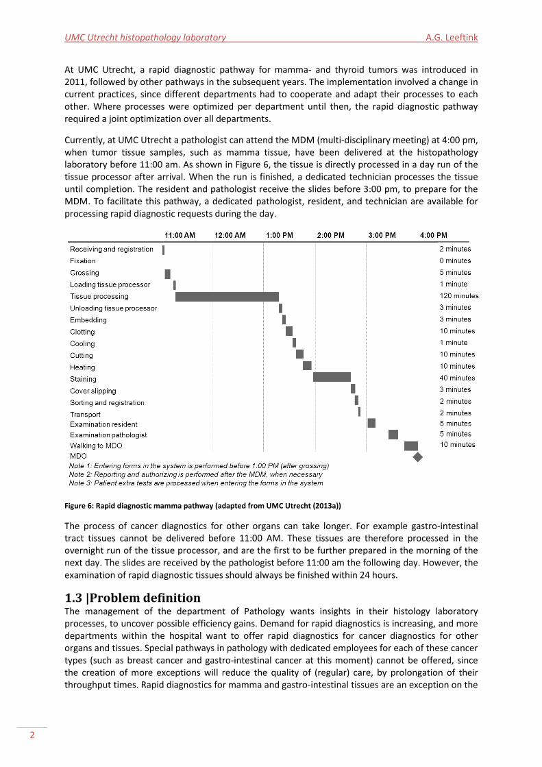
Currently, at UMC Utrecht a pathologist can attend the MDM (multi-disciplinary meeting) at 4:00 pm, when tumor tissue samples, such as mamma tissue, have been delivered at the histopathology laboratory before 11:00 am. As shown in Figure 6, the tissue is directly processed in a day run of the tissue processor after arrival. When the run is finished, a dedicated technician processes the tissue until completion. The resident and pathologist receive the slides before 3:00 pm, to prepare for the MDM. To facilitate this pathway, a dedicated pathologist, resident, and technician are available for processing rapid diagnostic requests during the day.
Figure 6: Rapid diagnostic mamma pathway (adapted from UMC Utrecht (2013a))
The process of cancer diagnostics for other organs can take longer. For example gastro-intestinal tract tissues cannot be delivered before 11:00 AM. These tissues are therefore processed in the overnight run of the tissue processor, and are the first to be further prepared in the morning of the next day. The slides are received by the pathologist before 11:00 am the following day. However, the examination of rapid diagnostic tissues should always be finished within 24 hours.
1.3 |Problem definition The management of the department of Pathology wants insights in their histology laboratory processes, to uncover possible efficiency gains. Demand for rapid diagnostics is increasing, and more departments within the hospital want to offer rapid diagnostics for cancer diagnostics for other organs and tissues. Special pathways in pathology with dedicated employees for each of these cancer types (such as breast cancer and gastro-intestinal cancer at this moment) cannot be offered, since the creation of more exceptions will reduce the quality of (regular) care, by prolongation of their throughput times. Rapid diagnostics for mamma and gastro-intestinal tissues are an exception on the

From rapid diagnostics to a rapid diagnosis A.G. Leeftink
3
regular processing at this moment, for example tissue processing is performed during the day for the mamma tissues only. Furthermore, it is known that reserving capacity for specific tissues results in a large reduction of performance for other (regular) samples (Zonderland et al., 2012, and Vanberkel et al., 2012). Research is needed to determine whether all processes can be equalized, such that rapid diagnostic tissues are not the exception anymore, but the standard.
The management of the department of Pathology has a great interest in this research, since service contracts for the tissue processing machines are expiring, and new investments need to be done. In their opinion, the optimization of the processes at the histopathology laboratory is largely influenced by the characteristics of the tissue processing machines. Therefore, optimizing the processes at the histopathology laboratory is not restricted to the currently available resources.
At the patient administration, the materials are received. Since more tissue samples arrive during the afternoon, two employees are available during the afternoon, while in the morning only one employee is present to register all incoming material.
At the histopathology laboratory, the processes are arranged to provide the pathologists and residents enough research and education time (UMC Utrecht, 2006). As a result, the cutting of tissue samples has to be finished before 1:00 PM, which causes a higher work pressure for the technicians during the morning, and a lower work pressure during the afternoon. The same accounts for the embedding technicians, since they have to embed all processed tissue in the morning, such that paraffin sections can be cut by the remaining technicians. Concluding, processes at the histopathology laboratory are planned to match pathologists’ agendas.
This results in the following problem statement:
Problem statement:
The performance of processes at the histopathology laboratory is negatively influenced by prioritizing the processing of rapid diagnostic tissues. There is a need for efficient processing of all processes instead of a selection of tissues.
1.4 |Objective and approach Research objective:
To review the histopathology laboratory operations, and develop and prospectively assess organizational interventions that aim to realize rapid diagnostics for all incoming tissue samples, in order to recommend a solution that organizes the processes so that a rapid diagnosis is realized for all tissue samples.
Currently, the histopathology laboratory is in the process of acquiring a new tissue processing machine. The analysis in this report should help the department of Pathology to assess the requirements for a new tissue processing machine.
This research objective is realized by answering the following research questions:
1. What is the workflow and performance of the regular tissue histopathology laboratory operations?
2. What is the workflow and performance of the rapid diagnostic tissue histopathology laboratory operations?
When designing an optimal processing pathway, the current situation should be well known. To review the histopathology laboratory operations, we analyze:
UMC Utrecht histopathology laboratory A.G. Leeftink
4
the system, by observing the processes,
the control of the system, by reviewing the resources of the system, and
the performance of the system, by considering the input, output, and (waiting) time in the system.
A core question is: ‘What is the influence of the rapid diagnostic processes on the regular processes?’
During this analysis we will use data from the laboratory management system (LMS), which records all tissue samples in all phases of the processes of the histopathology laboratory. The LMS provides data about tissue arrivals and start times of processing of tissues at several workstations. We also use data from the tissue processors, and the staining machine, about batch quantities and durations. Furthermore, we will use observations to check if the data from LMS is reliable, and to complement missing data. An extension of existing UMC Utrecht formats for observing histopathology laboratory operations is used for these observations.
As a performance measure for regular tissue processing we use the throughput time (TPT), since this measure is used as a key performance indicator of the regular histopathology laboratory operations (Royal College of Pathologists, 2012, and Pathologie, 2013).
As a performance measure for rapid diagnostic tissue processing we use the percentage of rapid diagnostic evaluations on time. The time of the MDM can be considered as given, since this moment is a joint scheduled moment of multiple departments, and out of scope of this research. Rapid diagnostic tissue samples do not necessarily need to be examined as soon as possible, since they are left unused until the MDM. However, they do need to be examined before the MDM.
During this analysis, we consider the whole process at the histopathology laboratory, from the receiving of materials to the examination of the pathologists. We only consider the HE-staining to be in scope, the process of extra inquiries and special staining is out of scope for the time-being.
3. How can the regular operations and rapid diagnostic operations be integrated, using the current resources available?
4. How can the regular operations and rapid diagnostic operations be integrated, allowing resource investments?
The ideal situation is a situation in which no unnecessary waiting occurs, in which rapid diagnostics are no exception, and in which the workload for all employees is equally divided over the days. Therefore, distinction has to be made between necessary and unnecessary waiting.
From interviews with pathologists, residents, and technicians, and from the information on the standard protocols of all histopathology processes from the intranet, information on necessary waiting is derived. Observations and questionnaires are performed to get a better understanding on the relation between the number of tissue samples and the needed time of tissue processing, since this relation is unknown.
To answer these questions, literature is studied for improvement opportunities to move the current operations to the ideal situation. Furthermore, we conduct several interviews to obtain possibilities for improvement by technicians, residents, pathologists, and the management of pathology. Solutions are not limited to the current tissue processors. Therefore, different tissue processing machines are evaluated in this research question.
5. What are the computational effects of the selected approaches? 6. What steps are needed to implement the selected approaches?
From rapid diagnostics to a rapid diagnosis A.G. Leeftink
5
The most promising solutions from literature and interviews are subject to an in depth evaluation, since the solutions are designed for use in practice. For each solution we will analyze the corresponding workflow, batch quantities and batching rules, personnel schedules, etc. Those ideas are implemented in a computational model to be prospectively assessed. To evaluate the performance of the solutions, we will look at the performance of the regular tissue processing, the performance of the rapid diagnostic processing, and the impact on the system.
Finally, an implementation plan is described, wherein changes and risks are identified to assure the implementation in practice.
1.5 |Challenges This section discusses possible threats to the success of this research project.
Availability of data A mathematical model generates a great need for (detailed) process data. There is a wealth of data in various ICT systems, however, they have to be subtracted from these systems, which can be a challenge. During the duration of the project, there are several ICT implementations scheduled. This can cause the systems to (temporary) fail. Since data is gathered from these systems, this can significantly delay the project. Information on the scheduling of ICT changes should be gathered, to efficiently cope with this risk.
Lab manager The hierarchy at the histopathology laboratory is changing, since the lab manager has resigned. As from the 1st of May 2014, there will be a vacancy. This can cause the commitment to the project to reduce, since technicians are more concerned with managing the regular operations. Furthermore, introducing the new lab manager to the problem when introducing her to the department and laboratory, may lower the commitment and priority given to the project.
Tissue processing machine There are several tissue processors available on the market. These machines all have their own characteristics, such as processing times, the size of batches, but also on the use of chemicals. The last characteristic should be evaluated with the help of technicians. If we recommend a tissue processing machine that does not reach the required quality levels or uses a ´wrong´ type of chemicals, the machine will not be successfully implemented. Since this information requires knowledge of chemical processes and work experience, the selection of the machines should be done in cooperation with several technicians.

UMC Utrecht histopathology laboratory A.G. Leeftink
6
From rapid diagnostics to a rapid diagnosis A.G. Leeftink
7
Chapter 2 |Context analysis This chapter evaluates the workflow and performance of the histopathology laboratory, and provides an answer to the first and second research question. Upon this analysis, organizational interventions will be developed and assessed in the remaining chapters.
Section 2.1 describes the processes in the histopathology laboratory. Section 2.2 describes the resources involved. Section 2.3 describes the performance of the system, by addressing the input, output, (waiting) time in the system, and other previously identified performance indicators. The influence of the rapid diagnostic processes on the remaining processes is evaluated as well. We end with a conclusion in Section 2.4.
Recall that during this analysis, we consider the whole process at the histopathology laboratory, from the receiving of materials to the examination of the pathologists. We only consider the HE-staining to be in scope, the process of extra inquiries and special staining is out of scope for time-being.
2.1 |Process description This section evaluates the methodology used. Second the process flow and the staff characteristics are described. Thereafter, the specimen types that enter the system are evaluated, and we end with some general characteristics on input and output.
Methodology To fully understand the system and its control, processes at the histopathology laboratory were observed, and interviews with different employees were conducted. Data from an earlier project on the performance of the histopathology laboratory were analyzed, together with data from the LMS (laboratory management system) and U-DPS (the national pathology database). Combined, these methods resulted in an in depth understanding of the processes and the value adding activities of the histopathology laboratory. The flow charts of the processes, which were the deliverables of this step of the research, are validated by experienced technicians and the lab manager.
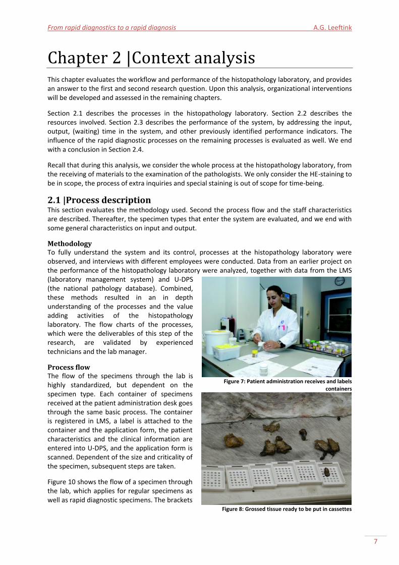
Process flow The flow of the specimens through the lab is highly standardized, but dependent on the specimen type. Each container of specimens received at the patient administration desk goes through the same basic process. The container is registered in LMS, a label is attached to the container and the application form, the patient characteristics and the clinical information are entered into U-DPS, and the application form is scanned. Dependent of the size and criticality of the specimen, subsequent steps are taken.
Figure 10 shows the flow of a specimen through the lab, which applies for regular specimens as well as rapid diagnostic specimens. The brackets
Figure 7: Patient administration receives and labels
containers
Figure 8: Grossed tissue ready to be put in cassettes
UMC Utrecht histopathology laboratory A.G. Leeftink
8
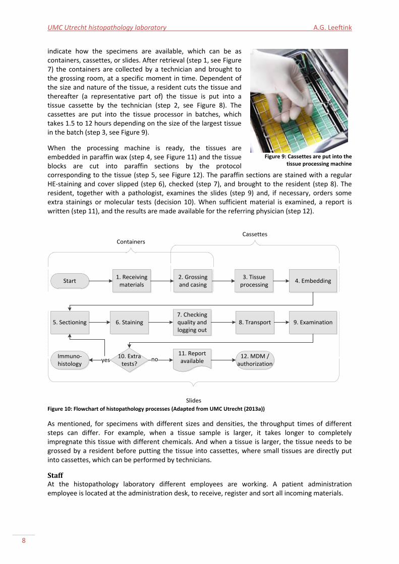
indicate how the specimens are available, which can be as containers, cassettes, or slides. After retrieval (step 1, see Figure 7) the containers are collected by a technician and brought to the grossing room, at a specific moment in time. Dependent of the size and nature of the tissue, a resident cuts the tissue and thereafter (a representative part of) the tissue is put into a tissue cassette by the technician (step 2, see Figure 8). The cassettes are put into the tissue processor in batches, which takes 1.5 to 12 hours depending on the size of the largest tissue in the batch (step 3, see Figure 9).
When the processing machine is ready, the tissues are embedded in paraffin wax (step 4, see Figure 11) and the tissue blocks are cut into paraffin sections by the protocol corresponding to the tissue (step 5, see Figure 12). The paraffin sections are stained with a regular HE-staining and cover slipped (step 6), checked (step 7), and brought to the resident (step 8). The resident, together with a pathologist, examines the slides (step 9) and, if necessary, orders some extra stainings or molecular tests (decision 10). When sufficient material is examined, a report is written (step 11), and the results are made available for the referring physician (step 12).
Start1. Receiving
materials2. Grossing and casing
3. Tissue processing
4. Embedding
5. Sectioning 6. Staining7. Checking quality and logging out
8. Transport 9. Examination
10. Extra tests?
11. Report availablenoImmuno-
histologyyes
12. MDM / authorization
14-8-2014 - 21-8-2014
Containers
14-8-2014 - 21-8-2014
Cassettes
14-8-2014 - 21-8-2014
Slides
5. Cutting slides
Figure 10: Flowchart of histopathology processes (Adapted from UMC Utrecht (2013a))
As mentioned, for specimens with different sizes and densities, the throughput times of different steps can differ. For example, when a tissue sample is larger, it takes longer to completely impregnate this tissue with different chemicals. And when a tissue is larger, the tissue needs to be grossed by a resident before putting the tissue into cassettes, where small tissues are directly put into cassettes, which can be performed by technicians.
Staff At the histopathology laboratory different employees are working. A patient administration employee is located at the administration desk, to receive, register and sort all incoming materials.
Figure 9: Cassettes are put into the
tissue processing machine
From rapid diagnostics to a rapid diagnosis A.G. Leeftink
9
In the grossing area, residents and technicians are working together. Residents gross the tissues, assisted by technicians. When the slides are ready, they are brought to the residents by the technicians, for examination. The resident checks the slides, and examines them together with the pathologist.
Next to assisting the residents with the grossing, technicians are also involved in embedding the tissues, cutting paraffin sections (‘sectioning’), staining, and the final quality check. They are also responsible for putting the small tissues into cassettes. Technicians have one task a day, but rotate between all tasks over the days.
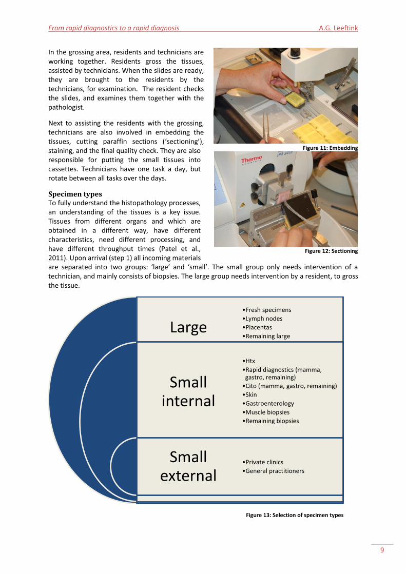
Specimen types To fully understand the histopathology processes, an understanding of the tissues is a key issue. Tissues from different organs and which are obtained in a different way, have different characteristics, need different processing, and have different throughput times (Patel et al., 2011). Upon arrival (step 1) all incoming materials are separated into two groups: ‘large’ and ‘small’. The small group only needs intervention of a technician, and mainly consists of biopsies. The large group needs intervention by a resident, to gross the tissue.
Figure 13: Selection of specimen types
Large
Small internal
Small external
•Fresh specimens
•Lymph nodes
•Placentas
•Remaining large
•Htx
•Rapid diagnostics (mamma, gastro, remaining)
•Cito (mamma, gastro, remaining)
•Skin
•Gastroenterology
•Muscle biopsies
•Remaining biopsies
•Private clinics
•General practitioners
Figure 11: Embedding
Figure 12: Sectioning
UMC Utrecht histopathology laboratory A.G. Leeftink
10
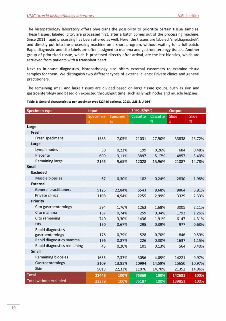
The histopathology laboratory offers physicians the possibility to prioritize certain tissue samples. These tissues, labeled ‘cito’, are processed first, after a batch comes out of the processing machine. Since 2011, rapid processing has been offered as well. Here, the tissues are labeled ‘sneldiagnostiek’, and directly put into the processing machine on a short program, without waiting for a full batch. Rapid diagnostic and cito labels are often assigned to mamma and gastroenterology tissues. Another group of prioritized tissue, which is processed directly after arrival, are the htx biopsies, which are retrieved from patients with a transplant heart.
Next to in-house diagnostics, histopathology also offers external customers to examine tissue samples for them. We distinguish two different types of external clients: Private clinics and general practitioners.
The remaining small and large tissues are divided based on large tissue groups, such as skin and gastroenterology and based on expected throughput time, such as lymph nodes and muscle biopsies.
Table 1: General characteristics per specimen type (22446 patients, 2013, LMS & U-DPS)
Specimen type Input Throughput Output
Specimen #
Specimen %
Cassette #
Cassette %
Slide #
Slide %
Large
Fresh
Fresh specimens 1583 7,05% 21031 27,90% 33838 23,72% Large
Lymph nodes 50 0,22% 199 0,26% 684 0,48% Placenta 699 3,11% 3897 5,17% 4857 3,40% Remaining large 2166 9,65% 12028 15,96% 21087 14,78%
Small
Excluded
Muscle biopsies 67 0,30% 182 0,24% 2830 1,98% External
General practitioners 5126 22,84% 6543 8,68% 9864 6,91% Private clinics 1108 4,94% 2255 2,99% 3329 2,33%
Priority
Cito gastroenterology 394 1,76% 1263 1,68% 3005 2,11% Cito mamma 167 0,74% 259 0,34% 1793 1,26% Cito remaining 740 3,30% 1436 1,91% 6147 4,31% Htx 150 0,67% 295 0,39% 977 0,68% Rapid diagnostics gastroenterology 178 0,79% 528 0,70% 846 0,59% Rapid diagnostics mamma 196 0,87% 226 0,30% 1637 1,15% Rapid diagnostics remaining 45 0,20% 101 0,13% 564 0,40%
Small
Remaining biopsies 1655 7,37% 3056 4,05% 14221 9,97% Gastroenterology 3109 13,85% 10994 14,59% 15650 10,97% Skin 5013 22,33% 11076 14,70% 21352 14,96%
Total 22446 100% 75369 100% 142681 100%
Total without excluded 22379 100% 75187 100% 139851 100%
From rapid diagnostics to a rapid diagnosis A.G. Leeftink
11
Based on these evaluations, we identified together with the laboratory manager a selection of specimen types, as shown in Figure 13.
General characteristics Table 1 displays general characteristics on each of the specimen types. The input equals the number of patients that enters the system. Therefore, it can be calculated by identifying the number of unique LMS registrations. The output equals the number of slides that leave the system. Therefore, it can be calculated by identifying the number of slides per LMS registration. During the process from input to output, the specimens in the containers of the patients are grossed and cased into cassettes. These cassettes are subject to the tissue processing and embedding process.
In the remainder of our research, muscle biopsies are excluded from our analyses. This is a very small group, with abnormal characteristics, such as an enormous amount of slides. As seen in the general characteristics only 0.3% of the received specimens are a muscle biopsy. The average throughput time is 37 days, which is more than six times the average throughput time. This is caused by very extensive testing within the different resources of the department of Pathology.
Based on observations and interviews, it is known that tissue processing takes place during the night before the first paraffin sections of that specimen are cut. However, when the paraffin sections are cut at the same date as the arrival and registration, there has been run an extra tissue processing run during that day. Biopsies received before 11:00 AM can be processed in a tissue processing run during the day.
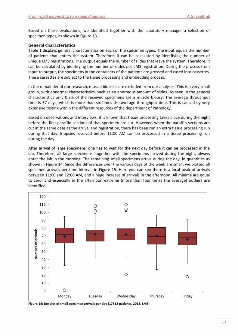
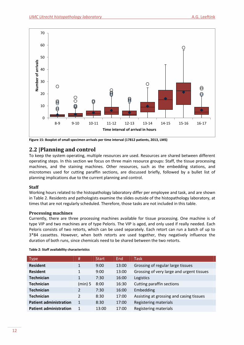
After arrival of large specimens, one has to wait for the next day before it can be processed in the lab. Therefore, all large specimens, together with the specimens arrived during the night, always enter the lab in the morning. The remaining small specimens arrive during the day, in quantities as shown in Figure 14. Since the differences over the various days of the week are small, we plotted all specimen arrivals per time interval in Figure 15. Here you can see there is a local peak of arrivals between 11:00 and 12:00 AM, and a huge increase of arrivals in the afternoon. All minima are equal to zero, and especially in the afternoon extreme (more than four times the average) outliers are identified.
Figure 14: Boxplot of small specimen arrivals per day (17812 patients, 2013, LMS)
0
10
20
30
40
50
60
70
80
90
100
110
120
Monday Tuesday Wednesday Thursday Friday
Nu
mb
er
of
arri
vals
UMC Utrecht histopathology laboratory A.G. Leeftink
12
Figure 15: Boxplot of small specimen arrivals per time interval (17812 patients, 2013, LMS)
2.2 |Planning and control To keep the system operating, multiple resources are used. Resources are shared between different operating steps. In this section we focus on three main resource groups: Staff, the tissue processing machines, and the staining machines. Other resources, such as the embedding stations, and microtomes used for cutting paraffin sections, are discussed briefly, followed by a bullet list of planning implications due to the current planning and control.
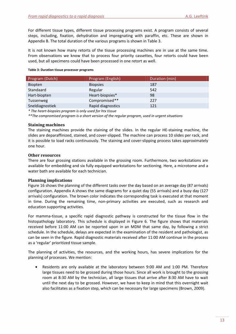
Staff Working hours related to the histopathology laboratory differ per employee and task, and are shown in Table 2. Residents and pathologists examine the slides outside of the histopathology laboratory, at times that are not regularly scheduled. Therefore, those tasks are not included in this table.
Processing machines Currently, there are three processing machines available for tissue processing. One machine is of type VIP and two machines are of type Peloris. The VIP is aged, and only used if really needed. Each Peloris consists of two retorts, which can be used separately. Each retort can run a batch of up to 3*84 cassettes. However, when both retorts are used together, they negatively influence the duration of both runs, since chemicals need to be shared between the two retorts.
Table 2: Staff availability characteristics
Type # Start End Task
Resident 1 9:00 13:00 Grossing of regular large tissues
Resident 1 9:00 13:00 Grossing of very large and urgent tissues
Technician 1 7:30 16:00 Logistics
Technician (min) 5 8:00 16:30 Cutting paraffin sections
Technician 2 7:30 16:00 Embedding
Technician 2 8:30 17:00 Assisting at grossing and casing tissues
Patient administration 1 8:30 17:00 Registering materials
Patient administration 1 13:00 17:00 Registering materials
0
10
20
30
40
50
60
70
8-9 9-10 10-11 11-12 12-13 13-14 14-15 15-16 16-17
Nu
mb
er
of
arri
vals
Time interval of arrival in hours
From rapid diagnostics to a rapid diagnosis A.G. Leeftink
13
For different tissue types, different tissue processing programs exist. A program consists of several steps, including, fixation, dehydration and impregnating with paraffin, etc. These are shown in Appendix B. The total duration of the various programs is shown in Table 3.
It is not known how many retorts of the tissue processing machines are in use at the same time. From observations we know that to process four priority cassettes, four retorts could have been used, but all specimens could have been processed in one retort as well.
Table 3: Duration tissue processor programs
Program (Dutch) Program (English) Duration (min)
Biopten Biopsies 187 Standaard Regular 542 Hart-biopten Heart-biopsies* 98 Tussenweg Compromised** 227 Sneldiagnostiek Rapid diagnostics 121 * The heart-biopsies program is only used for htx tissue **The compromised program is a short version of the regular program, used in urgent situations
Staining machines The staining machines provide the staining of the slides. In the regular HE-staining machine, the slides are deparaffinized, stained, and cover-slipped. The machine can process 10 slides per rack, and it is possible to load racks continuously. The staining and cover-slipping process takes approximately one hour.
Other resources There are four grossing stations available in the grossing room. Furthermore, two workstations are available for embedding and six fully equipped workstations for sectioning. Here, a microtome and a water bath are available for each technician.
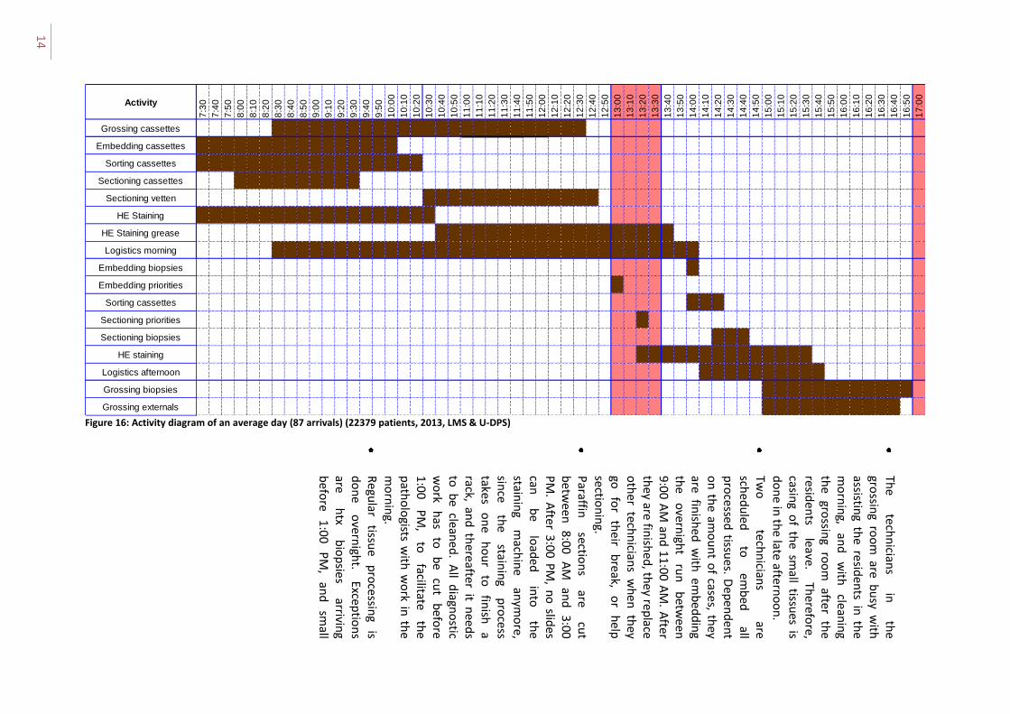
Planning implications Figure 16 shows the planning of the different tasks over the day based on an average day (87 arrivals) configuration. Appendix A shows the same diagrams for a quiet day (55 arrivals) and a busy day (127 arrivals) configuration. The brown color indicates the corresponding task is executed at that moment in time. During the remaining time, non-primary activities are executed, such as research and education supporting activities.
For mamma-tissue, a specific rapid diagnostic pathway is constructed for the tissue flow in the histopathology laboratory. This schedule is displayed in Figure 6. The figure shows that materials received before 11:00 AM can be reported upon in an MDM that same day, by following a strict schedule. In the schedule, delays are expected in the examination of the resident and pathologist, as can be seen in the figure. Rapid diagnostic materials received after 11:00 AM continue in the process as a ‘regular’ prioritized tissue sample.
The planning of activities, the resources, and the working hours, has severe implications for the planning of processes. We mention:
Residents are only available at the laboratory between 9:00 AM and 1:00 PM. Therefore large tissues need to be grossed during those hours. Since all work is brought to the grossing room at 8:30 AM by the technician, all large tissues that arrive after 8:30 AM have to wait until the next day to be grossed. However, we have to keep in mind that this overnight wait also facilitates as a fixation step, which can be necessary for large specimens (Brown, 2009).
14
Figure 16: Activity diagram of an average day (87 arrivals) (22379 patients, 2013, LMS & U-DPS)
Activity
7:3
0
7:4
0
7:5
0
8:0
0
8:1
0
8:2
0
8:3
0
8:4
0
8:5
0
9:0
0
9:1
0
9:2
0
9:3
0
9:4
0
9:5
0
10
:00
10
:10
10
:20
10
:30
10
:40
10
:50
11
:00
11
:10
11
:20
11
:30
11
:40
11
:50
12
:00
12
:10
12
:20
12
:30
12
:40
12
:50
13
:00
13
:10
13
:20
13
:30
13
:40
13
:50
14
:00
14
:10
14
:20
14
:30
14
:40
14
:50
15
:00
15
:10
15
:20
15
:30
15
:40
15
:50
16
:00
16
:10
16
:20
16
:30
16
:40
16
:50
17
:00
Grossing cassettes
Embedding cassettes ### ### ### ### ### ### ### ### ### ### ### ### ### ### ### ### ### ### ### ### ### ### ### ### ### ### ### ### ### ### ### ### ### ### ### ### ### ### ### ### ### ### ### ### ### ### ### ### ### ### ### ### ### ### ### ### ### ###
Sorting cassettes ### ### ### ### ### ### ### ### ### ### ### ### ### ### ### ### ### ### ### ### ### ### ### ### ### ### ### ### ### ### ### ### ### ### ### ### ### ### ### ### ### ### ### ### ### ### ### ### ### ### ### ### ### ### ### ### ### ###
Sectioning cassettes 9:39 9:39 9:39 9:39 9:39 9:39 9:39 9:39 9:39 9:39 9:39 9:39 9:39 9:39 9:39 9:39 9:39 9:39 9:39 9:39 9:39 9:39 9:39 9:39 9:39 9:39 9:39 9:39 9:39 9:39 9:39 9:39 9:39 9:39 9:39 9:39 9:39 9:39 9:39 9:39 9:39 9:39 9:39 9:39 9:39 9:39 9:39 9:39 9:39 9:39 9:39 9:39 9:39 9:39 9:39 9:39 9:39 9:39
Sectioning vetten ### ### ### ### ### ### ### ### ### ### ### ### ### ### ### ### ### ### ### ### ### ### ### ### ### ### ### ### ### ### ### ### ### ### ### ### ### ### ### ### ### ### ### ### ### ### ### ### ### ### ### ### ### ### ### ### ### ###
HE Staining ### ### ### ### ### ### ### ### ### ### ### ### ### ### ### ### ### ### ### ### ### ### ### ### ### ### ### ### ### ### ### ### ### ### ### ### ### ### ### ### ### ### ### ### ### ### ### ### ### ### ### ### ### ### ### ### ### ###
HE Staining grease ### ### ### ### ### ### ### ### ### ### ### ### ### ### ### ### ### ### ### ### ### ### ### ### ### ### ### ### ### ### ### ### ### ### ### ### ### ### ### ### ### ### ### ### ### ### ### ### ### ### ### ### ### ### ### ### ### ###
Logistics morning ### ### ### ### ### ### ### ### ### ### ### ### ### ### ### ### ### ### ### ### ### ### ### ### ### ### ### ### ### ### ### ### ### ### ### ### ### ### ### ### ### ### ### ### ### ### ### ### ### ### ### ### ### ### ### ### ### ###
Embedding biopsies 0,6 0,6 0,6 0,6 0,6 0,6 0,6 0,6 0,6 0,6 0,6 0,6 0,6 0,6 0,6 0,6 0,6 0,6 0,6 0,6 0,6 0,6 0,6 0,6 0,6 0,6 0,6 0,6 0,6 0,6 0,6 0,6 0,6 0,6 0,6 0,6 0,6 0,6 0,6 0,6 0,6 0,6 0,6 0,6 0,6 0,6 0,6 0,6 0,6 0,6 0,6 0,6 0,6 0,6 0,6 0,6 0,6 0,6
Embedding priorities 0,5 0,5 0,5 0,5 0,5 0,5 0,5 0,5 0,5 0,5 0,5 0,5 0,5 0,5 0,5 0,5 0,5 0,5 0,5 0,5 0,5 0,5 0,5 0,5 0,5 0,5 0,5 0,5 0,5 0,5 0,5 0,5 0,5 0,5 0,5 0,5 0,5 0,5 0,5 0,5 0,5 0,5 0,5 0,5 0,5 0,5 0,5 0,5 0,5 0,5 0,5 0,5 0,5 0,5 0,5 0,5 0,5 0,5
Sorting cassettes 0,6 0,6 0,6 0,6 0,6 0,6 0,6 0,6 0,6 0,6 0,6 0,6 0,6 0,6 0,6 0,6 0,6 0,6 0,6 0,6 0,6 0,6 0,6 0,6 0,6 0,6 0,6 0,6 0,6 0,6 0,6 0,6 0,6 0,6 0,6 0,6 0,6 0,6 0,6 0,6 0,6 0,6 0,6 0,6 0,6 0,6 0,6 0,6 0,6 0,6 0,6 0,6 0,6 0,6 0,6 0,6 0,6 0,6
Sectioning priorities 0,6 0,6 0,6 0,6 0,6 0,6 0,6 0,6 0,6 0,6 0,6 0,6 0,6 0,6 0,6 0,6 0,6 0,6 0,6 0,6 0,6 0,6 0,6 0,6 0,6 0,6 0,6 0,6 0,6 0,6 0,6 0,6 0,6 0,6 0,6 0,6 0,6 0,6 0,6 0,6 0,6 0,6 0,6 0,6 0,6 0,6 0,6 0,6 0,6 0,6 0,6 0,6 0,6 0,6 0,6 0,6 0,6 0,6
Sectioning biopsies 0,6 0,6 0,6 0,6 0,6 0,6 0,6 0,6 0,6 0,6 0,6 0,6 0,6 0,6 0,6 0,6 0,6 0,6 0,6 0,6 0,6 0,6 0,6 0,6 0,6 0,6 0,6 0,6 0,6 0,6 0,6 0,6 0,6 0,6 0,6 0,6 0,6 0,6 0,6 0,6 0,6 0,6 0,6 0,6 0,6 0,6 0,6 0,6 0,6 0,6 0,6 0,6 0,6 0,6 0,6 0,6 0,6 0,6
HE staining 0,6 0,6 0,6 0,6 0,6 0,6 0,6 0,6 0,6 0,6 0,6 0,6 0,6 0,6 0,6 0,6 0,6 0,6 0,6 0,6 0,6 0,6 0,6 0,6 0,6 0,6 0,6 0,6 0,6 0,6 0,6 0,6 0,6 0,6 0,6 0,6 0,6 0,6 0,6 0,6 0,6 ### 0,6 0,6 0,6 0,6 0,6 0,6 0,6 0,6 0,6 0,6 0,6 0,6 0,6 0,6 0,6 0,6
Logistics afternoon 0,7 0,7 0,7 0,7 0,7 0,7 0,7 0,7 0,7 0,7 0,7 0,7 0,7 0,7 0,7 0,7 0,7 0,7 0,7 0,7 0,7 0,7 0,7 0,7 0,7 0,7 0,7 0,7 0,7 0,7 0,7 0,7 0,7 0,7 0,7 0,7 0,7 0,7 0,7 0,7 0,7 0,7 0,7 0,7 0,7 0,7 0,7 0,7 0,7 0,7 0,7 0,7 0,7 0,7 0,7 0,7 0,7 0,7
Grossing biopsies
Grossing externals 0,7 0,7 0,7 0,7 0,7 0,7 0,7 0,7 0,7 0,7 0,7 0,7 0,7 0,7 0,7 0,7 0,7 0,7 0,7 0,7 0,7 0,7 0,7 0,7 0,7 0,7 0,7 0,7 0,7 0,7 0,7 0,7 0,7 0,7 0,7 0,7 0,7 0,7 0,7 0,7 0,7 0,7 0,7 0,7 0,7 0,7 0,7 0,7 0,7 0,7 0,7 0,7 0,7 0,7 0,7 0,7 0,7 0,7
The
techn
icians
in
the
grossin
g roo
m are b
usy w
ith
assisting th
e residen
ts in th
e m
orn
ing,
and
w
ith
cleanin
g th
e gro
ssing
roo
m
after th
e resid
ents
leave. Th
erefore,
casing o
f the sm
all tissues is
do
ne in
the late aftern
oo
n.
Two
te
chn
icians
are sch
edu
led
to
emb
ed
all p
rocessed
tissues. D
epen
den
t o
n th
e amo
un
t of cases, th
ey are fin
ished
with
emb
edd
ing
the
overn
ight
run
b
etwee
n
9:0
0 AM
and
11
:00
AM
. After
they are fin
ished
, they rep
lace o
ther tech
nician
s wh
en th
ey go
fo
r th
eir b
reak, o
r h
elp
section
ing.
Paraffin
sectio
ns
are cu
t b
etween
8:00
A
M
and
3:00
PM
. Afte
r 3:00 P
M, n
o slid
es can
b
e lo
aded
in
to
the
stainin
g m
achin
e an
ymo
re, sin
ce th
e stain
ing
pro
cess take
s o
ne
ho
ur
to
finish
a
rack, and
thereafter it n
eeds
to b
e cleaned
. All d
iagno
stic w
ork
has
to
be
cut
befo
re 1
:00
P
M,
to
facilitate th
e p
atho
logists w
ith w
ork in
the
mo
rnin
g.
Regu
lar tissu
e p
rocessin
g is
do
ne
overn
ight.
Exceptio
ns
are h
tx b
iop
sies arrivin
g b
efore
1:0
0
PM
, an
d
small
From rapid diagnostics to a rapid diagnosis A.G. Leeftink
15
When more than +/- 15 biopsies are available at the administration desk before 10:00 AM, a biopsy processing program should be run during the day. However, from observations it is known that the implementation of this rule depends on the technician in the grossing room, and the patient administration.
Due to the logistics in the hospital, it frequently happens that a large batch of biopsy specimens arrives in the late afternoon. At that time, the working processes are comparable with the ‘busy day’ configuration, even though the rest of the day was not busy at all. This causes a need for extra work outside working hours, as seen in Figure 40 in Appendix A, while during other moments of the same day this work could have been done.
At many stages in the process, tissue samples, cassettes, and slides are sorted. This sorting starts at the administration desk, where small tissues are mixed in order to prevent contamination of cases in the grossing room. Furthermore, prioritized cassettes are sorted before they are put into the processing machine, and all cases with the same patient number are put together. This way, the embedding technicians can embed the prioritized cases first. Before the slides are cut, all paraffin sections are sorted by their number, since only completed pathology numbers are delivered to the technicians cutting paraffin sections. After being sectioned and stained, the slides are sorted by their number again, to be sent to the resident for examination.
2.3 |Performance This section first considers the data gathering methods. Second, performance indicators are identified in literature and the performance on these indicators is evaluated. As performance indicators, we consider throughput time and workload.
Data gathering methods Performance indicators are obtained from academic literature, from hospital documentation, such as the departmental yearly report, and from interviews with the personnel. Hereby, we focus on indicators actually used in UMC Utrecht, and applicable to the situation in the histopathology laboratory.
Figure 17: Time registration moments
3-3-2014 4-3-2014
4-3-2014Print slidelabel
3-3-2014Print cassette
3-3-2014Registration in LMS
4-3-2014Log out slide
4-3-2014Log out patient
3-3-2014 - 3-3-2014Arrival and registration3-3-2014 - 3-3-2014
Grossing and casing
3-3-2014 - 4-3-2014Tissue processing
3-3-2014Timestamp
4-3-2014 - 4-3-2014Embedding4-3-2014 - 4-3-2014
Cutting paraffin sections
4-3-2014 - 4-3-2014Staining slides
4-3-2014Day border
3-3-2014Day border
3-3-2014Day border
3-3-2014Day border
Legend
4-3-2014
Possible day border
UMC Utrecht histopathology laboratory A.G. Leeftink
16
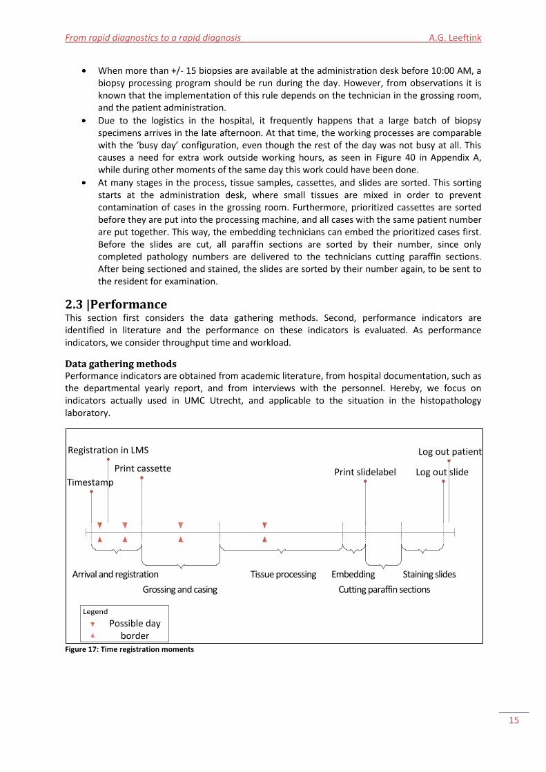
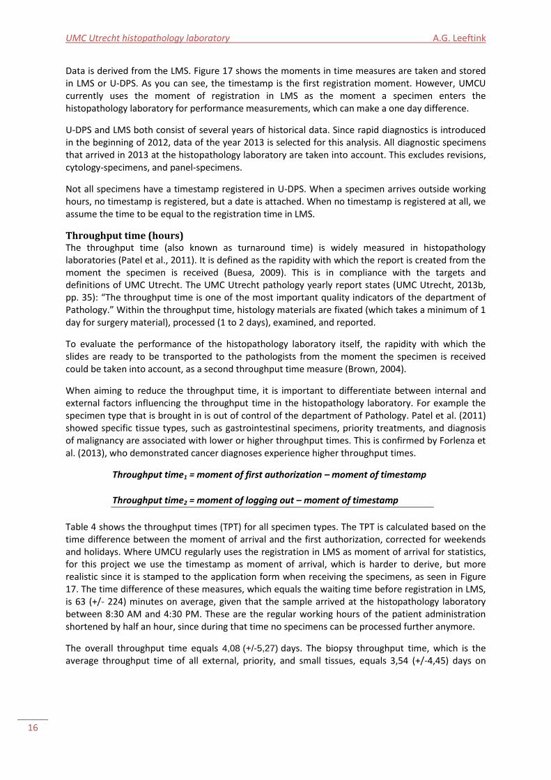
Data is derived from the LMS. Figure 17 shows the moments in time measures are taken and stored in LMS or U-DPS. As you can see, the timestamp is the first registration moment. However, UMCU currently uses the moment of registration in LMS as the moment a specimen enters the histopathology laboratory for performance measurements, which can make a one day difference.
U-DPS and LMS both consist of several years of historical data. Since rapid diagnostics is introduced in the beginning of 2012, data of the year 2013 is selected for this analysis. All diagnostic specimens that arrived in 2013 at the histopathology laboratory are taken into account. This excludes revisions, cytology-specimens, and panel-specimens.
Not all specimens have a timestamp registered in U-DPS. When a specimen arrives outside working hours, no timestamp is registered, but a date is attached. When no timestamp is registered at all, we assume the time to be equal to the registration time in LMS.
Throughput time (hours) The throughput time (also known as turnaround time) is widely measured in histopathology laboratories (Patel et al., 2011). It is defined as the rapidity with which the report is created from the moment the specimen is received (Buesa, 2009). This is in compliance with the targets and definitions of UMC Utrecht. The UMC Utrecht pathology yearly report states (UMC Utrecht, 2013b, pp. 35): “The throughput time is one of the most important quality indicators of the department of Pathology.” Within the throughput time, histology materials are fixated (which takes a minimum of 1 day for surgery material), processed (1 to 2 days), examined, and reported.
To evaluate the performance of the histopathology laboratory itself, the rapidity with which the slides are ready to be transported to the pathologists from the moment the specimen is received could be taken into account, as a second throughput time measure (Brown, 2004).
When aiming to reduce the throughput time, it is important to differentiate between internal and external factors influencing the throughput time in the histopathology laboratory. For example the specimen type that is brought in is out of control of the department of Pathology. Patel et al. (2011) showed specific tissue types, such as gastrointestinal specimens, priority treatments, and diagnosis of malignancy are associated with lower or higher throughput times. This is confirmed by Forlenza et al. (2013), who demonstrated cancer diagnoses experience higher throughput times.
Throughput time1 = moment of first authorization – moment of timestamp
Throughput time2 = moment of logging out – moment of timestamp
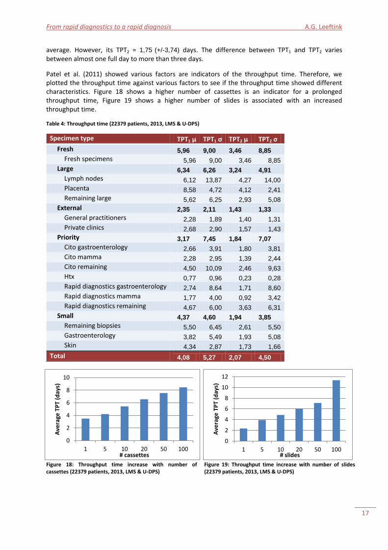
Table 4 shows the throughput times (TPT) for all specimen types. The TPT is calculated based on the time difference between the moment of arrival and the first authorization, corrected for weekends and holidays. Where UMCU regularly uses the registration in LMS as moment of arrival for statistics, for this project we use the timestamp as moment of arrival, which is harder to derive, but more realistic since it is stamped to the application form when receiving the specimens, as seen in Figure 17. The time difference of these measures, which equals the waiting time before registration in LMS, is 63 (+/- 224) minutes on average, given that the sample arrived at the histopathology laboratory between 8:30 AM and 4:30 PM. These are the regular working hours of the patient administration shortened by half an hour, since during that time no specimens can be processed further anymore.
The overall throughput time equals 4,08 (+/-5,27) days. The biopsy throughput time, which is the average throughput time of all external, priority, and small tissues, equals 3,54 (+/-4,45) days on
From rapid diagnostics to a rapid diagnosis A.G. Leeftink
17
average. However, its TPT2 = 1,75 (+/-3,74) days. The difference between TPT1 and TPT2 varies between almost one full day to more than three days.
Patel et al. (2011) showed various factors are indicators of the throughput time. Therefore, we plotted the throughput time against various factors to see if the throughput time showed different characteristics. Figure 18 shows a higher number of cassettes is an indicator for a prolonged throughput time, Figure 19 shows a higher number of slides is associated with an increased throughput time.
Table 4: Throughput time (22379 patients, 2013, LMS & U-DPS)
Specimen type TPT1 μ TPT1 σ TPT2 μ TPT2 σ
Fresh 5,96 9,00 3,46 8,85
Fresh specimens 5,96 9,00 3,46 8,85
Large 6,34 6,26 3,24 4,91
Lymph nodes 6,12 13,87 4,27 14,00
Placenta 8,58 4,72 4,12 2,41
Remaining large 5,62 6,25 2,93 5,08
External 2,35 2,11 1,43 1,33
General practitioners 2,28 1,89 1,40 1,31
Private clinics 2,68 2,90 1,57 1,43
Priority 3,17 7,45 1,84 7,07
Cito gastroenterology 2,66 3,91 1,80 3,81
Cito mamma 2,28 2,95 1,39 2,44
Cito remaining 4,50 10,09 2,46 9,63
Htx 0,77 0,96 0,23 0,28
Rapid diagnostics gastroenterology 2,74 8,64 1,71 8,60
Rapid diagnostics mamma 1,77 4,00 0,92 3,42
Rapid diagnostics remaining 4,67 6,00 3,63 6,31
Small 4,37 4,60 1,94 3,85
Remaining biopsies 5,50 6,45 2,61 5,50
Gastroenterology 3,82 5,49 1,93 5,08
Skin 4,34 2,87 1,73 1,66
Total 4,08 5,27 2,07 4,50
Figure 18: Throughput time increase with number of cassettes (22379 patients, 2013, LMS & U-DPS)
Figure 19: Throughput time increase with number of slides (22379 patients, 2013, LMS & U-DPS)
0
2
4
6
8
10
1 5 10 20 50 100
Ave
rage
TP
T (d
ays)
# cassettes
0
2
4
6
8
10
12
1 5 10 20 50 100
Ave
rage
TP
T (d
ays)
# slides
UMC Utrecht histopathology laboratory A.G. Leeftink
18
Percentage authorized within x days (%) In the Netherlands, the percentage of specimens reviewed on time is a common performance indicator, for which the throughput time is used. Hereby, ‘reviewed’ includes the time from arrival to an authorization by the pathologist. Different definitions of ‘on time’ are used by the department of Pathology of UMC Utrecht and the Royal College of Pathologists’ – 10 working days (UMC Utrecht, 2013b) and 7 working days (Royal College of Pathologists, 2012) respectively.
In UMC Utrecht, the KPI norm of the histopathology laboratory is to authorize 90% of the incoming internal specimens within 10 working days. Furthermore, the external skin specimens arrived before 3:00 PM should be authorized within 4 working days on average, which includes the specimens from general practitioners. Since private clinics also submit mamma specimens, which frequently involve extra tests and longer processing, a different target is agreed upon with them: 80% of the specimens within 6 working days.
Specimen specific targets are set for a few specific specimen types, such as rapid diagnostics and htx specimens. 90% of the rapid diagnostics specimens received before 11 o’clock, and the htx specimens should be authorized the same day, since they will be presented in the MDM the same afternoon. For cito tissues, there is no clear target norm. However, they have to be timely authorized.
Percentage of materials authorized within x days =
% of incoming specimens with TPT1 < x days
Table 5 shows the percentage of specimens with a TPT within the same day (UMC Utrecht target for htx and rapid diagnostics), and less than 1, 2, 4 (the target for external specimens), 6 (the target for private clinics specimens), 7 (the Royal College of Pathologists’ target for biopsies), and 10 days (the UMC Utrecht overall target). Table 5 shows the key performance indicator of 90% of the specimens, including biopsies and tissues requiring decalcification, finished within 10 working days is met for
Table 5: Percentage authorized on time per specimen type (22379 patients, 2013, LMS & U-DPS)
Specimen type Same day 1 day 2 days 4 days 6 days 7 days 10 days
Biopsies remaining 0% 3% 16% 45% 70% 79% 91%
Cito gastroenterology 3% 23% 59% 89% 93% 95% 97%
Cito mamma 1% 23% 69% 90% 96% 97% 98%
Cito remaining 2% 9% 33% 68% 86% 89% 93%
Fresh specimens 0% 5% 11% 41% 66% 77% 90%
Gastroenterology 0% 3% 24% 71% 89% 92% 97%
General practitioners 0% 6% 47% 91% 96% 97% 99%
Htx 51% 77% 93% 99% 99% 99% 100%
Lymph nodes 0% 0% 18% 58% 80% 84% 94%
Placenta 0% 0% 0% 7% 31% 43% 71%
Private clinics 0% 6% 43% 88% 95% 96% 98%
Rapid diagnostics gastroenterology 6% 28% 70% 89% 94% 96% 98%
Rapid diagnostics mamma 44% 57% 81% 92% 95% 96% 97%
Rapid diagnostics remaining 11% 20% 47% 62% 78% 80% 87%
Remaining large 0% 2% 8% 45% 70% 79% 92%
Skin 0% 2% 14% 56% 79% 86% 97%
Total 1% 6% 27% 65% 82% 87% 95%

From rapid diagnostics to a rapid diagnosis A.G. Leeftink
19
almost all specimen types, except for placentas. This discrepancy can be explained by the fact that the placentas are diagnosed for a specific hospital research project, require a prolonged fixation time before tissue processing is possible, and are non-urgent. The Royal College of Pathologists’ throughput time baseline is set to a 90% authorization of diagnosed biopsies within 7 days after the biopsy, and for other tissue types, excluding tissues requiring decalcification, within 10 days after the procedure (Royal College of Pathologists, 2012). Since the moment the tissue is taken from the patient is unknown, we use the moment of arrival at the histopathology laboratory. It is already shown that, even when including decalcification tissues, the baseline of within 10 days is met for most specimen types. The KPI of 90% of all biopsies authorized within 7 days is not met for specific biopsy specimen types, such as the remaining biopsies, remaining citos, and remaining rapid diagnostics. One of the reasons is the small size of these groups, which makes one outlier already influences the performance. However, when grouped together, the overall biopsy rate it is met (91%). In this analysis, large gastroenterology and skin excisions are also included as biopsies, for data sampling reasons.
As Table 5 showed, 91% of the specimens received from a general practitioner are authorized within the norm of 4 days, with an average TPT of 2,28 (+/-1,89) days. 95% of the specimens from private clinics are authorized within 6 days. The norms for external specimens are therefore met.
Table 6 shows the percentage of specimens ready for transport to the pathologist on time, to evaluate the performance of the histopathology laboratory itself. Table 6 shows a relatively high percentage of rapid diagnostics remaining specimens that are not logged out within two days. Since the remaining rapid diagnostics tissues are often brought in after the 11:00 AM deadline, the tissues are processed during the night, which often already causes a one-day delay, and includes the same treatment priorities as the remaining cito tissues.
Comparing Table 5 and Table 6, the largest differences can be seen in the first two days. Where the vast majority of slides are brought to the (resident) pathologist within two to four days, the examination of these slides usually takes more time. Part of this delay can be explained by the fact that UMC Utrecht is a teaching hospital with educational duties. This can cause a minor delay, since a
Table 6: Percentage ready for transportation on time per specimen type (22379 patients, 2013, LMS & U-DPS)
Specimen type Same day 1 day 2 days 4 days 6 days 7 days 10 days
Biopsies remaining 1% 28% 56% 88% 95% 96% 98%
Cito gastroenterology 6% 61% 85% 94% 95% 96% 98%
Cito mamma 2% 72% 95% 96% 97% 98% 98%
Cito remaining 6% 49% 73% 92% 95% 96% 96%
Fresh specimens 0% 24% 46% 79% 89% 92% 96%
Gastroenterology 0% 39% 79% 96% 98% 98% 99%
General practitioners 0% 19% 90% 99% 99% 99% 100%
Htx 88% 96% 99% 100% 100% 100% 100%
Lymph nodes 0% 20% 46% 84% 94% 96% 98%
Placenta 0% 1% 2% 56% 88% 91% 96%
Private clinics 0% 18% 83% 97% 98% 99% 99%
Rapid diagnostics gastroenterology 15% 78% 94% 98% 98% 98% 98%
Rapid diagnostics mamma 85% 90% 92% 94% 96% 97% 98%
Rapid diagnostics remaining 27% 47% 62% 76% 80% 82% 87%
Remaining large 0% 8% 50% 86% 93% 95% 98%
Skin 0% 31% 76% 96% 99% 99% 100%
Total 2% 28% 72% 93% 97% 97% 98%
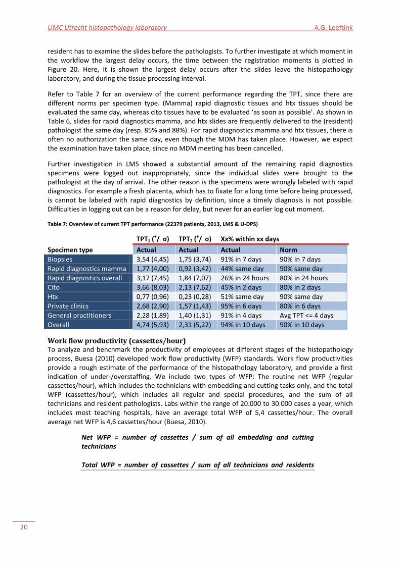
UMC Utrecht histopathology laboratory A.G. Leeftink
20
resident has to examine the slides before the pathologists. To further investigate at which moment in the workflow the largest delay occurs, the time between the registration moments is plotted in Figure 20. Here, it is shown the largest delay occurs after the slides leave the histopathology laboratory, and during the tissue processing interval.
Refer to Table 7 for an overview of the current performance regarding the TPT, since there are different norms per specimen type. (Mamma) rapid diagnostic tissues and htx tissues should be evaluated the same day, whereas cito tissues have to be evaluated ‘as soon as possible’. As shown in Table 6, slides for rapid diagnostics mamma, and htx slides are frequently delivered to the (resident) pathologist the same day (resp. 85% and 88%). For rapid diagnostics mamma and htx tissues, there is often no authorization the same day, even though the MDM has taken place. However, we expect the examination have taken place, since no MDM meeting has been cancelled.
Further investigation in LMS showed a substantial amount of the remaining rapid diagnostics specimens were logged out inappropriately, since the individual slides were brought to the pathologist at the day of arrival. The other reason is the specimens were wrongly labeled with rapid diagnostics. For example a fresh placenta, which has to fixate for a long time before being processed, is cannot be labeled with rapid diagnostics by definition, since a timely diagnosis is not possible. Difficulties in logging out can be a reason for delay, but never for an earlier log out moment.
Table 7: Overview of current TPT performance (22379 patients, 2013, LMS & U-DPS)
Specimen type
TPT1 (+/- σ) TPT2 (
+/- σ) Xx% within xx days
Actual Actual Actual Norm
Biopsies 3,54 (4,45) 1,75 (3,74) 91% in 7 days 90% in 7 days
Rapid diagnostics mamma 1,77 (4,00) 0,92 (3,42) 44% same day 90% same day
Rapid diagnostics overall 3,17 (7,45) 1,84 (7,07) 26% in 24 hours 80% in 24 hours
Cito 3,66 (8,03) 2,13 (7,62) 45% in 2 days 80% in 2 days
Htx 0,77 (0,96) 0,23 (0,28) 51% same day 90% same day
Private clinics 2,68 (2,90) 1,57 (1,43) 95% in 6 days 80% in 6 days
General practitioners 2,28 (1,89) 1,40 (1,31) 91% in 4 days Avg TPT <= 4 days
Overall 4,74 (5,93) 2,31 (5,22) 94% in 10 days 90% in 10 days
Work flow productivity (cassettes/hour) To analyze and benchmark the productivity of employees at different stages of the histopathology process, Buesa (2010) developed work flow productivity (WFP) standards. Work flow productivities provide a rough estimate of the performance of the histopathology laboratory, and provide a first indication of under-/overstaffing. We include two types of WFP: The routine net WFP (regular cassettes/hour), which includes the technicians with embedding and cutting tasks only, and the total WFP (cassettes/hour), which includes all regular and special procedures, and the sum of all technicians and resident pathologists. Labs within the range of 20.000 to 30.000 cases a year, which includes most teaching hospitals, have an average total WFP of 5,4 cassettes/hour. The overall average net WFP is 4,6 cassettes/hour (Buesa, 2010).
Net WFP = number of cassettes / sum of all embedding and cutting technicians
Total WFP = number of cassettes / sum of all technicians and residents

21
Figure 20: Average time between moments of registration (22379 patients, 2013, LMS & U-DPS)
0,00
0,50
1,00
1,50
2,00
2,50
3,00
3,50
Timestamp-LMS LMS-Print cassette Print cassette-Printslide label
Print slide label-Logout slide
Log out slide-Logout patient
Log out patient-1stauthorization
Tim
e in
day
s
Time interval
Average time between moments of registration
Biopsies
External
Large
Priority 24 hours
Priority same day
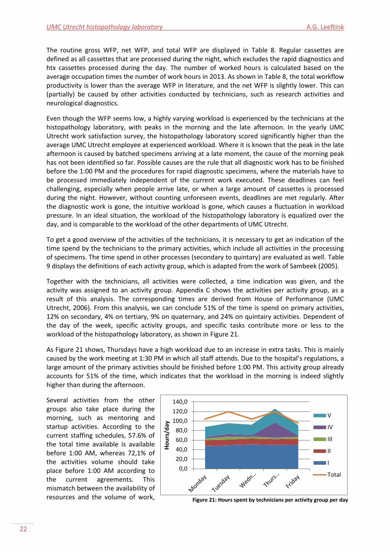
UMC Utrecht histopathology laboratory A.G. Leeftink
22
The routine gross WFP, net WFP, and total WFP are displayed in Table 8. Regular cassettes are defined as all cassettes that are processed during the night, which excludes the rapid diagnostics and htx cassettes processed during the day. The number of worked hours is calculated based on the average occupation times the number of work hours in 2013. As shown in Table 8, the total workflow productivity is lower than the average WFP in literature, and the net WFP is slightly lower. This can (partially) be caused by other activities conducted by technicians, such as research activities and neurological diagnostics.
Even though the WFP seems low, a highly varying workload is experienced by the technicians at the histopathology laboratory, with peaks in the morning and the late afternoon. In the yearly UMC Utrecht work satisfaction survey, the histopathology laboratory scored significantly higher than the average UMC Utrecht employee at experienced workload. Where it is known that the peak in the late afternoon is caused by batched specimens arriving at a late moment, the cause of the morning peak has not been identified so far. Possible causes are the rule that all diagnostic work has to be finished before the 1:00 PM and the procedures for rapid diagnostic specimens, where the materials have to be processed immediately independent of the current work executed. These deadlines can feel challenging, especially when people arrive late, or when a large amount of cassettes is processed during the night. However, without counting unforeseen events, deadlines are met regularly. After the diagnostic work is gone, the intuitive workload is gone, which causes a fluctuation in workload pressure. In an ideal situation, the workload of the histopathology laboratory is equalized over the day, and is comparable to the workload of the other departments of UMC Utrecht.
To get a good overview of the activities of the technicians, it is necessary to get an indication of the time spend by the technicians to the primary activities, which include all activities in the processing of specimens. The time spend in other processes (secondary to quintary) are evaluated as well. Table 9 displays the definitions of each activity group, which is adapted from the work of Sambeek (2005).
Together with the technicians, all activities were collected, a time indication was given, and the activity was assigned to an activity group. Appendix C shows the activities per activity group, as a result of this analysis. The corresponding times are derived from House of Performance (UMC Utrecht, 2006). From this analysis, we can conclude 51% of the time is spend on primary activities, 12% on secondary, 4% on tertiary, 9% on quaternary, and 24% on quintairy activities. Dependent of the day of the week, specific activity groups, and specific tasks contribute more or less to the workload of the histopathology laboratory, as shown in Figure 21.
As Figure 21 shows, Thursdays have a high workload due to an increase in extra tasks. This is mainly caused by the work meeting at 1:30 PM in which all staff attends. Due to the hospital’s regulations, a large amount of the primary activities should be finished before 1:00 PM. This activity group already accounts for 51% of the time, which indicates that the workload in the morning is indeed slightly higher than during the afternoon.
Several activities from the other groups also take place during the morning, such as mentoring and startup activities. According to the current staffing schedules, 57.6% of the total time available is available before 1:00 AM, whereas 72,1% of the activities volume should take place before 1:00 AM according to the current agreements. This mismatch between the availability of resources and the volume of work,
0,0
20,0
40,0
60,0
80,0
100,0
120,0
140,0
Ho
urs
/day
V
IV
III
II
I
Total
Figure 21: Hours spent by technicians per activity group per day
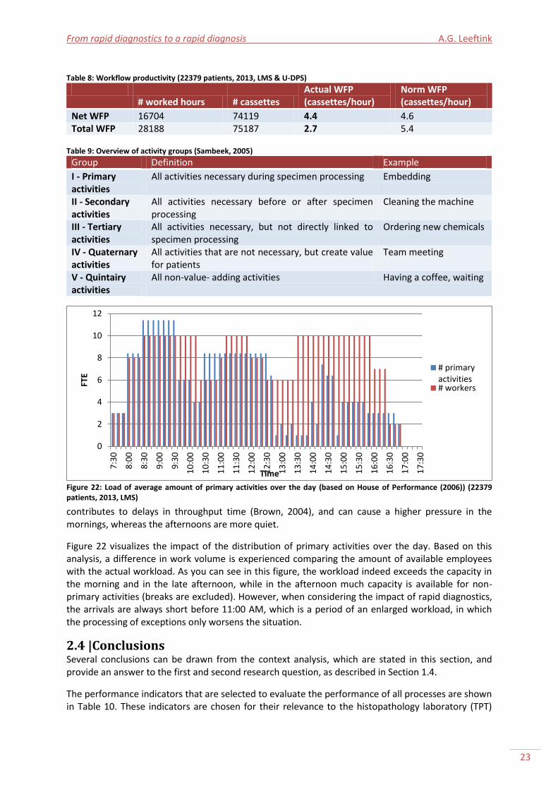
From rapid diagnostics to a rapid diagnosis A.G. Leeftink
23
contributes to delays in throughput time (Brown, 2004), and can cause a higher pressure in the mornings, whereas the afternoons are more quiet.
Figure 22 visualizes the impact of the distribution of primary activities over the day. Based on this analysis, a difference in work volume is experienced comparing the amount of available employees with the actual workload. As you can see in this figure, the workload indeed exceeds the capacity in the morning and in the late afternoon, while in the afternoon much capacity is available for non-primary activities (breaks are excluded). However, when considering the impact of rapid diagnostics, the arrivals are always short before 11:00 AM, which is a period of an enlarged workload, in which the processing of exceptions only worsens the situation.
2.4 |Conclusions Several conclusions can be drawn from the context analysis, which are stated in this section, and provide an answer to the first and second research question, as described in Section 1.4.
The performance indicators that are selected to evaluate the performance of all processes are shown in Table 10. These indicators are chosen for their relevance to the histopathology laboratory (TPT)
Table 8: Workflow productivity (22379 patients, 2013, LMS & U-DPS)
# worked hours # cassettes
Actual WFP (cassettes/hour)
Norm WFP (cassettes/hour)
Net WFP 16704 74119 4.4 4.6 Total WFP 28188 75187 2.7 5.4
Table 9: Overview of activity groups (Sambeek, 2005)
Group Definition Example
I - Primary activities
All activities necessary during specimen processing Embedding
II - Secondary activities
All activities necessary before or after specimen processing
Cleaning the machine
III - Tertiary activities
All activities necessary, but not directly linked to specimen processing
Ordering new chemicals
IV - Quaternary activities
All activities that are not necessary, but create value for patients
Team meeting
V - Quintairy activities
All non-value- adding activities Having a coffee, waiting
Figure 22: Load of average amount of primary activities over the day (based on House of Performance (2006)) (22379 patients, 2013, LMS)
0
2
4
6
8
10
12
7:3
0
8:0
0
8:3
0
9:0
0
9:3
0
10
:00
10
:30
11
:00
11
:30
12
:00
12
:30
13
:00
13
:30
14
:00
14
:30
15
:00
15
:30
16
:00
16
:30
17
:00
17
:30
FTE
Time
# primaryactivities# workers
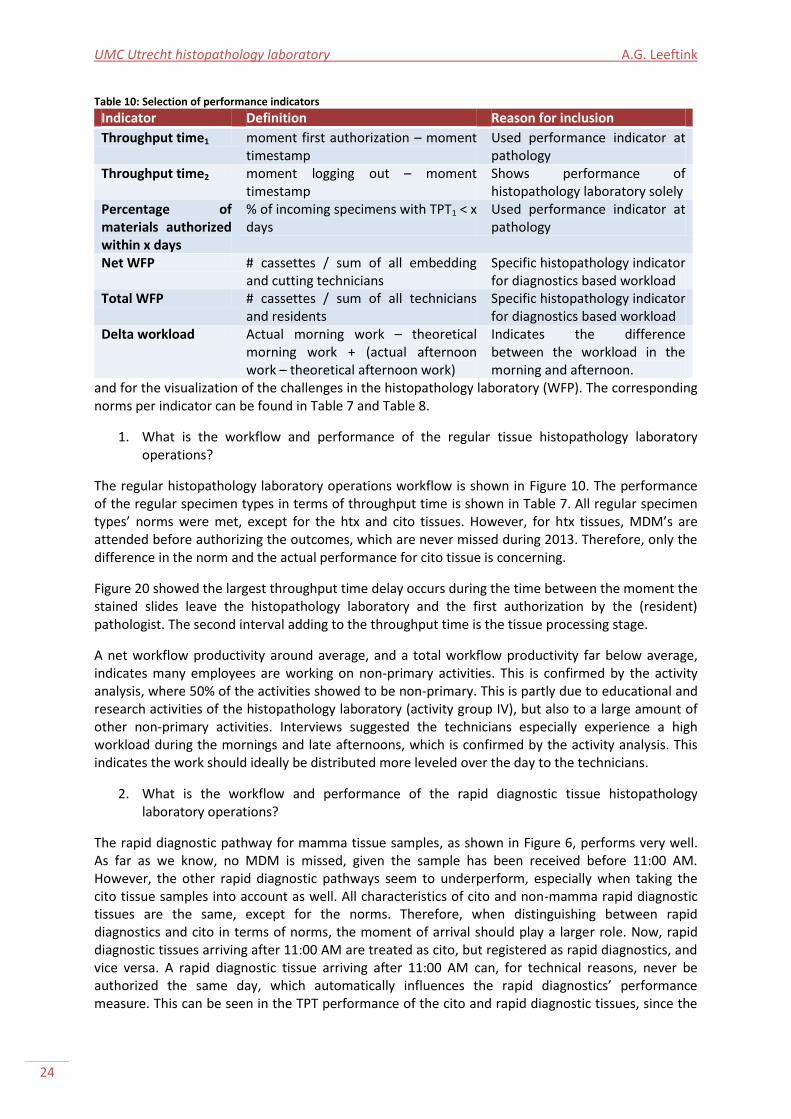
UMC Utrecht histopathology laboratory A.G. Leeftink
24
and for the visualization of the challenges in the histopathology laboratory (WFP). The corresponding norms per indicator can be found in Table 7 and Table 8.
1. What is the workflow and performance of the regular tissue histopathology laboratory operations?
The regular histopathology laboratory operations workflow is shown in Figure 10. The performance of the regular specimen types in terms of throughput time is shown in Table 7. All regular specimen types’ norms were met, except for the htx and cito tissues. However, for htx tissues, MDM’s are attended before authorizing the outcomes, which are never missed during 2013. Therefore, only the difference in the norm and the actual performance for cito tissue is concerning.
Figure 20 showed the largest throughput time delay occurs during the time between the moment the stained slides leave the histopathology laboratory and the first authorization by the (resident) pathologist. The second interval adding to the throughput time is the tissue processing stage.
A net workflow productivity around average, and a total workflow productivity far below average, indicates many employees are working on non-primary activities. This is confirmed by the activity analysis, where 50% of the activities showed to be non-primary. This is partly due to educational and research activities of the histopathology laboratory (activity group IV), but also to a large amount of other non-primary activities. Interviews suggested the technicians especially experience a high workload during the mornings and late afternoons, which is confirmed by the activity analysis. This indicates the work should ideally be distributed more leveled over the day to the technicians.
2. What is the workflow and performance of the rapid diagnostic tissue histopathology laboratory operations?
The rapid diagnostic pathway for mamma tissue samples, as shown in Figure 6, performs very well. As far as we know, no MDM is missed, given the sample has been received before 11:00 AM. However, the other rapid diagnostic pathways seem to underperform, especially when taking the cito tissue samples into account as well. All characteristics of cito and non-mamma rapid diagnostic tissues are the same, except for the norms. Therefore, when distinguishing between rapid diagnostics and cito in terms of norms, the moment of arrival should play a larger role. Now, rapid diagnostic tissues arriving after 11:00 AM are treated as cito, but registered as rapid diagnostics, and vice versa. A rapid diagnostic tissue arriving after 11:00 AM can, for technical reasons, never be authorized the same day, which automatically influences the rapid diagnostics’ performance measure. This can be seen in the TPT performance of the cito and rapid diagnostic tissues, since the
Table 10: Selection of performance indicators
Indicator Definition Reason for inclusion
Throughput time1 moment first authorization – moment timestamp
Used performance indicator at pathology
Throughput time2 moment logging out – moment timestamp
Shows performance of histopathology laboratory solely
Percentage of materials authorized within x days
% of incoming specimens with TPT1 < x days
Used performance indicator at pathology
Net WFP # cassettes / sum of all embedding and cutting technicians
Specific histopathology indicator for diagnostics based workload
Total WFP # cassettes / sum of all technicians and residents
Specific histopathology indicator for diagnostics based workload
Delta workload Actual morning work – theoretical morning work + (actual afternoon work – theoretical afternoon work)
Indicates the difference between the workload in the morning and afternoon.
From rapid diagnostics to a rapid diagnosis A.G. Leeftink
25
throughput times of mamma and gastroenterology citos are never more than the corresponding times of the rapid diagnostic tissues added with 0,75 day (which is the difference between an authorization at 5:00 PM and 11:00 AM the next morning).
Since rapid diagnostic specimens should arrive at the laboratory before 11:00 AM, rapid diagnostics especially disturb the morning activities. Even though the throughput times in the histopathology laboratory are met, the rapid diagnostic specimens disturb the regular, high workload, processes, where a lack of capacity is experienced already. The essence of the need for an integration of the regular diagnostics and rapid diagnostics is therefore a need for a more leveled workflow during the day, which will be the focus of the interventions in the remaining of this research.
The rapid diagnostic specimens that arrive after 11:00 AM currently do not perform well. The target of 80% within 1 day (24 hours) is not met, since the average TPT is more than 3 days, and only 24% is authorized within 24 hours. One of the causes is the large amount of extra tests that are often ordered for this patient group. Since the MDMs are, as far as we know, always met, we do not think the rapid diagnostic pathways for non-mamma specimens should be further investigated.
In the remainder of this research, we consider rapid diagnostics, cito, and htx specimens together as priority specimens.

UMC Utrecht histopathology laboratory A.G. Leeftink
26
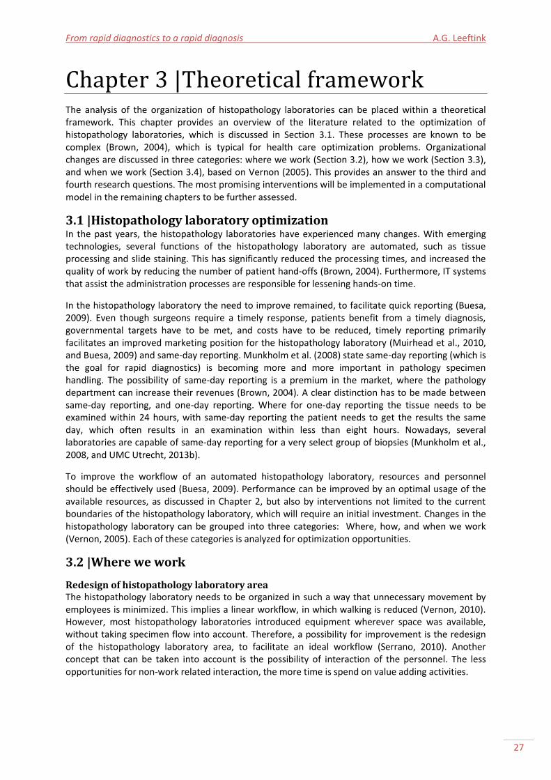
From rapid diagnostics to a rapid diagnosis A.G. Leeftink
27
Chapter 3 |Theoretical framework The analysis of the organization of histopathology laboratories can be placed within a theoretical framework. This chapter provides an overview of the literature related to the optimization of histopathology laboratories, which is discussed in Section 3.1. These processes are known to be complex (Brown, 2004), which is typical for health care optimization problems. Organizational changes are discussed in three categories: where we work (Section 3.2), how we work (Section 3.3), and when we work (Section 3.4), based on Vernon (2005). This provides an answer to the third and fourth research questions. The most promising interventions will be implemented in a computational model in the remaining chapters to be further assessed.
3.1 |Histopathology laboratory optimization In the past years, the histopathology laboratories have experienced many changes. With emerging technologies, several functions of the histopathology laboratory are automated, such as tissue processing and slide staining. This has significantly reduced the processing times, and increased the quality of work by reducing the number of patient hand-offs (Brown, 2004). Furthermore, IT systems that assist the administration processes are responsible for lessening hands-on time.
In the histopathology laboratory the need to improve remained, to facilitate quick reporting (Buesa, 2009). Even though surgeons require a timely response, patients benefit from a timely diagnosis, governmental targets have to be met, and costs have to be reduced, timely reporting primarily facilitates an improved marketing position for the histopathology laboratory (Muirhead et al., 2010, and Buesa, 2009) and same-day reporting. Munkholm et al. (2008) state same-day reporting (which is the goal for rapid diagnostics) is becoming more and more important in pathology specimen handling. The possibility of same-day reporting is a premium in the market, where the pathology department can increase their revenues (Brown, 2004). A clear distinction has to be made between same-day reporting, and one-day reporting. Where for one-day reporting the tissue needs to be examined within 24 hours, with same-day reporting the patient needs to get the results the same day, which often results in an examination within less than eight hours. Nowadays, several laboratories are capable of same-day reporting for a very select group of biopsies (Munkholm et al., 2008, and UMC Utrecht, 2013b).
To improve the workflow of an automated histopathology laboratory, resources and personnel should be effectively used (Buesa, 2009). Performance can be improved by an optimal usage of the available resources, as discussed in Chapter 2, but also by interventions not limited to the current boundaries of the histopathology laboratory, which will require an initial investment. Changes in the histopathology laboratory can be grouped into three categories: Where, how, and when we work (Vernon, 2005). Each of these categories is analyzed for optimization opportunities.
3.2 |Where we work
Redesign of histopathology laboratory area The histopathology laboratory needs to be organized in such a way that unnecessary movement by employees is minimized. This implies a linear workflow, in which walking is reduced (Vernon, 2010). However, most histopathology laboratories introduced equipment wherever space was available, without taking specimen flow into account. Therefore, a possibility for improvement is the redesign of the histopathology laboratory area, to facilitate an ideal workflow (Serrano, 2010). Another concept that can be taken into account is the possibility of interaction of the personnel. The less opportunities for non-work related interaction, the more time is spend on value adding activities.
UMC Utrecht histopathology laboratory A.G. Leeftink
28
3.3 |How we work
Tissue processing methods Where automation of histopathology processes was the main focus for the past years, recent literature on histopathology optimization by changing the means is primarily focused on tissue processing methods (Buesa, 2007). Tissue processing, performed by a tissue processos (an example is shown in Figure 23) is the most time-consuming process in the histopathology laboratory, since tissue processing methods used for large tissues lasts for at least eight hours. Therefore, conventional tissue processing is done overnight. The advantage of overnight tissue processing is the utilization of the night hours. The disadvantage is a standard 1-day diagnostic delay (Munkholm, 2008, and Vernon, 2005).
The improvement of tissue processing has two objectives: shortening the processing time, and optimizing the infiltration of tissue. Where the second one is (partially) achieved nowadays by sophisticated tissue processing machines, the focus of literature has been on the first objective (Buesa, 2007).
The processing time of tissue processing instruments can be improved by using microwave technologies. Specific types of microwave assisted tissue processing machines exist that enable continuous processing, where cassettes do not need to be processed in batches (Buesa, 2007). However, in a test at the histopathology laboratory in UMC Utrecht, the quality of the tissues processed by microwave assisted continuous tissue processing instruments currently available is proven to be resulting low quality slides. Therefore, we will not investigate the opportunities of the use of this type of equipment.
To find the right tissue processing machine for a lab, other factors have to be taken into account. First, the size of the machine is important, since laboratories are often crowded, and experience space shortages (Buesa, 2009). Second, the (re)supply of chemicals is important, since dealing with chemicals manually influences the quality of work (Brown, 2009). Third, the selection of the right machine depends on the throughput times of the other processes in the laboratory, since processing during the day is only feasible when other tasks can also be finished earlier (Buesa, 2007). Ideally, batch sizes and durations should be adaptable to the tissue size. Last, the cost-effectiveness of the machine has to be evaluated, since a tissue processing machine is a capital expenditure (Buesa, 2007).
Batching A second change in the way of work can be found in the reduction of batching steps. Tissues are batched and re-batched in several stages of the workflow. However, re-batching of blocks, for example after embedding, wastes time and prevents a truly continuous process (Buesa, 2009). In the ideal situation, all materials should be continuously processed, which eliminates all batching from the process. However, before transporting the slides to the pathologist, a quality check should be built into the process, to ensure the quality of the slides, and match the slides with the blocks and the application form (Vernon, 2010).
Quick wins A key lean principle is the introduction of standardized work. By reducing unnecessary exceptions, work becomes more standardized. Standardized work allows for more constant decision making, is well documented, and results in more steady performance and order of tasks (Serrano, 2010).
Figure 23: Tissue processor
From rapid diagnostics to a rapid diagnosis A.G. Leeftink
29
Another lean principle is the removal of duplicated steps. Unnecessary checking of blocks against the application forms and unnecessary sorting of blocks should be removed from the processes (Brown, 2004).
3.4 |When we work
Tissue processing during the day Tissue processing regularly takes place during the night in an eight hour program. Here, biopsies are usually processed together with the other specimens. However, biopsy processing needs less time, since the tissues are smaller. The current processing standard results in over processing and excessive dehydration of biopsies, but also in under processing and incomplete dehydration of larger specimens. A biopsy program should run for one to three hours, dependent on the tissue processing machine. Ideally, tissues are processed with tailored programs, adjusted to their size, thickness, and fixation level (Brown, 2009). The implementation of multiple tissue processing runs during the day is suggested for biopsies and other fixated small specimens, to increase the quality of the patient material processed, and to facilitate one-day reporting. Different tissue processing programs during the day result in a change of workflow, since dehydrated tissue becomes available for embedding during the day. Tissue processing rules should be configured on the laboratories workflow, to optimize the throughput time (Munkholm et al., 2008).
Rescheduling shifts Major throughput time improvements can be reached by rescheduling shifts (Ribé et al., 1998). We saw that a traditional one-day delay for histopathology diagnosis is expected due to overnight tissue processing. However, schedules of (resident) pathologists and technicians accommodate this one day wait for pathologic diagnosis. The implications for the histopathology laboratory are a buzzy workplace in the morning, with lower work pressure during the afternoon (Buesa, 2009). An adaption of the shifts not only accommodates a more continuous flow with lowered peak moments, but also a multitude of cases can be examined within one day. However, the reporting activities of the pathologists have to shift from early in the morning towards the afternoon (Vernon, 2005).
Based on a lean project, Serrano et al. (2010) used a staggered staffing schedule, with the first technicians arriving at 4:00 AM, to directly process the cassettes when the overnight tissue processing machine is finished. Buesa (2009) suggests a pull process, in which the tissue processing machine is scheduled to finish two hours (which corresponds with their embedding, cutting, and staining duration) before the (resident) pathologists are ready to start reporting, with corresponding technician schedules.
In all cases, the actual corresponding improvement in throughput time has not been mentioned.
3.5 |Conclusions Concluding, several options for improvement can be found in literature. We distinguish projects using the current resources available, projects with the need for (resource) investments, and quick wins. This enables to evaluate possibilities for interventions based on the criteria of the third and fourth research questions, as described in Section 1.4.
3. How can the regular operations and rapid diagnostic operations be integrated, using the current resources available?
No investment The projects with no need for a large resource investment, relate to ‘how we work’. First, the tissue processor program configuration can be optimized, by looking at tissue processing moments during the day, different tissue processing programs for different specimen types, and staggered tissue processing.

UMC Utrecht histopathology laboratory A.G. Leeftink
30
Second, shifts can be rescheduled to provide an optimized staffing schedule. Extending the working hours, staggering the shifts, and staffing in alignment with the tissue processing moments and/or the pathologists’ agendas are possibilities to consider.
4. How can the regular operations and rapid diagnostic operations be integrated, allowing resource investments?
Investment The projects with a need for a financial investment are related to the tissue processing machine itself. Research should be done to see which possibilities there are for obtaining tissue processing equipment which suits the workflow of a specific histopathology laboratory. Several options, ranging from multiple smaller machines, up to one large machine, need to be evaluated. Second, the redesign of the laboratory can be considered to optimize the specimen routing. Most histopathology laboratories introduced equipment wherever space was available, without taking specimen routing into account.
Quick wins Third, there are quick wins to consider. This includes standardizing work activities, such as the registration of rapid diagnostics in LMS, or removing unnecessary sorting and checking.
Scope In the remainder of this research, we will further investigate the possibilities to improve the histopathology laboratory operations by rescheduling the shifts and working hours of the resources. Furthermore, we will investigate the consequences of working with different tissue processors and their corresponding programs.

From rapid diagnostics to a rapid diagnosis A.G. Leeftink
31
Chapter 4 |Model description In this chapter computational program is developed and verified, to prospectively assess organizational interventions that aim to realize rapid diagnostics for all incoming tissue samples. These organizational interventions, resulting from Chapter 3, will be prospectively assessed using this program in the next chapters.
First, the methodology is described in Section 4.1. The remaining sections consider the steps in model design and verification as described in the methodology section. We end with a conclusion in Section 4.7.
4.1 |Methodology To prospectively assess the interventions described in Chapter 3, without actually changing the histopathology laboratory operations, we build a mathematical model. A model is a tool that is used to assess different interventions on consequences, without changing the system itself (Law, 2007). We build our model using the methodology described in Law (2007). This method includes the following steps, as shown in Figure 24:
1. Problem statement and research question, 2. Conceptual design, 3. Data gathering, 4. Mathematical formulation, 5. Verification, 6. Validation, 7. Experimentation, 8. Analysis, 9. Conclusions and recommendations.
The experimentation, analysis, and examination will be performed in the remaining chapters. The problem statement and research questions are already described in Chapter 1. However, with the insights gathered in the previous chapters, we can classify the problem on hand more specifically. The scheduling problem with parallel batching resources in the histopathology laboratory is comparable to scheduling problems in the chemical industry and scheduling of burn-in oven processes, due to the batching resources with large processing times in the middle of the chain of serial processes. This industry is also known as the process industry (Kallrath, 2002).
The scheduling problem on hand is very complex. It is known that scheduling multi-stage processes is more complex than single-stage plant scheduling. Furthermore, scheduling multiproduct processes is more complex than single process scheduling (Gupta and Karimi, 2003). The histopathology laboratory modeling problem is a scheduling problem in a multi-stage, multiproduct environment. We consider the problem as a flow shop problem, where all specimens are processed in all stages, in a predefined order of stages (Méndez et al., 2006).
Figure 24: Steps in a modeling study, based on Law (2007)
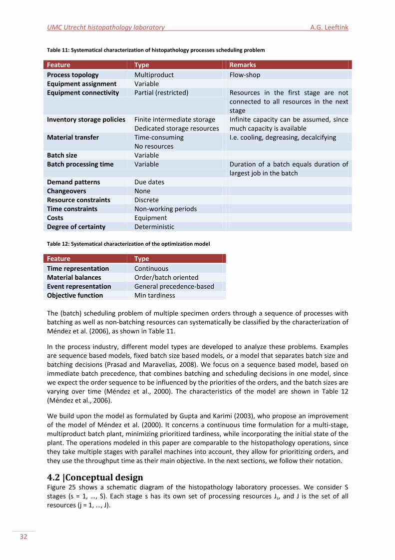
UMC Utrecht histopathology laboratory A.G. Leeftink
32
Table 11: Systematical characterization of histopathology processes scheduling problem
Feature Type Remarks
Process topology Multiproduct Flow-shop Equipment assignment Variable Equipment connectivity Partial (restricted) Resources in the first stage are not
connected to all resources in the next stage
Inventory storage policies Finite intermediate storage Dedicated storage resources
Infinite capacity can be assumed, since much capacity is available
Material transfer Time-consuming No resources
I.e. cooling, degreasing, decalcifying
Batch size Variable Batch processing time Variable Duration of a batch equals duration of
largest job in the batch Demand patterns Due dates Changeovers None Resource constraints Discrete Time constraints Non-working periods Costs Equipment Degree of certainty Deterministic Table 12: Systematical characterization of the optimization model
Feature Type
Time representation Continuous Material balances Order/batch oriented Event representation General precedence-based Objective function Min tardiness The (batch) scheduling problem of multiple specimen orders through a sequence of processes with batching as well as non-batching resources can systematically be classified by the characterization of Méndez et al. (2006), as shown in Table 11.
In the process industry, different model types are developed to analyze these problems. Examples are sequence based models, fixed batch size based models, or a model that separates batch size and batching decisions (Prasad and Maravelias, 2008). We focus on a sequence based model, based on immediate batch precedence, that combines batching and scheduling decisions in one model, since we expect the order sequence to be influenced by the priorities of the orders, and the batch sizes are varying over time (Méndez et al., 2000). The characteristics of the model are shown in Table 12 (Méndez et al., 2006).
We build upon the model as formulated by Gupta and Karimi (2003), who propose an improvement of the model of Méndez et al. (2000). It concerns a continuous time formulation for a multi-stage, multiproduct batch plant, minimizing prioritized tardiness, while incorporating the initial state of the plant. The operations modeled in this paper are comparable to the histopathology operations, since they take multiple stages with parallel machines into account, they allow for prioritizing orders, and they use the throughput time as their main objective. In the next sections, we follow their notation.
4.2 |Conceptual design Figure 25 shows a schematic diagram of the histopathology laboratory processes. We consider S stages (s = 1, …, S). Each stage s has its own set of processing resources Js, and J is the set of all resources (j = 1, …, J).

From rapid diagnostics to a rapid diagnosis A.G. Leeftink
33
Stage 1: non-identical processors
Stage 2: batch processors
Stage 4: parallel processors
Stage 3: parallel processors
Legend
Units
Orders
Resident
Technician
Figure 25: Schematic diagram of the histopathology system, S=4, J=13.
The output of the system is driven by orders, which all have their own known processing times in different stages. We consider I different orders (i = 1, ..., I) with known target due dates di. An order consists of a specific specimen type g (g = 1, …, G).
Let Ij be the subset ( ) of orders that can be processed by a resource j, and Jis be the subset
( ) of resources that can process order i in stage s. This differs per order, since for example large specimens cannot be processed on a batch processor with a short processing time. Let tij be the processing time of order i on resource j, and tbj be the processing time of a batch on resource j.
Restrictions are present upon the sequencing of orders on resources; Not all orders can be handled by each resource, and it is possible that two orders i and i' have completely different subsets of resources in a stage s, i.e. the intersection of Jis and Ji’s is empty. Let NCis be the subset of orders that cannot use any of the processing resources suitable for i in stage s, i.e. .
Resource j can start processing after time URTj, the resource release time. Order i is released at time ORTi, the order release time. During the planning horizon, we consider A nights (a = 1,…,A). During the time intervals [NW1aj, NW2a + URTj] corresponding with night a, non-batching resources are unavailable and batch processing resources cannot start a new operation.
Since the characteristics for batch processors differ from parallel processing resources, the continuous time approach with sequencing orders is more complicated the batch processing stages,
UMC Utrecht histopathology laboratory A.G. Leeftink
34
due to the need for complicated constraints regarding variable processing times and resource limitations (Mendez et al., 2006). A discrete time model offers a less complex solution, even though some flexibility will be lost. Therefore, we introduce B different batch processing moments (b = 1, …, B) per batching resource, which are the preselected batch processing moments that can start at a certain resource j. Let parameter bsjb define the starting time of batch b on resource j.
The following assumptions apply:
1. The maximum batch size of a batch processing resource is unlimited. Non-batch processing resources can process a maximum of one order at the same time.
2. Since the size of orders varies in each stage, let fij be a scaling factor for the order size of order i on resource j. A small example: If order 1 of type ‘large’ has 8 cassettes in the tissue processor, which makes the scaling factor f1,tissue processor = 8. Furthermore, from these 8 cassettes, 10 slides are prepared by a technician, which makes the scaling factor in the sectioning stage f1, sectioning technician= 10.
3. An order can only be processed by one resource at a time, and when started, it should be finished completely by that resource before starting another operation. Processing is non-preemptive.
4. There is unlimited intermediate storage between all stages. 5. All model parameters, such as processing times, release times, and due dates, are
deterministic and known beforehand. 6. Non-batch processing resources are unavailable during nights. An order should be
completely finished processing on a resource before the start of the night, or be started after the night. Pre-emption during the night is not allowed. Batch processing resources are available during night when started before the start of the night hours of that resource.
7. The states of all orders and resources are known at time zero.
The following data is needed as input for the mathematical model:
1. A set of resources (j ∈ J), divided in batching (j ∈ Jbatch) and non-batching (j ∈ Jnon-batch) resources, with release times.
2. A set of stages (s ∈ S) with corresponding processing resources (j ∈ Js). 3. A set of specimen types (g ∈ G). 4. A set of orders (i ∈ I) with release times, due dates, processing times, transfer times,
priorities, order size scaling factors, stage routing, and specimen types. 5. The planning horizon and a corresponding set of nights (a ∈ A) with known start and end
times [NW1aj, NW2a + URTj] for each resource (j ∈ J).
All required data is available from LMS, U-DPS, House of Performance, and observations.
The developed model should assign each order to a processing resource in each stage, it should sequence the orders on each resource, and it should determine the processing start times of all orders in each stage. The output of the model is a schedule of all orders for each resource in use. From this schedule, the workload per resource, the start processing times per order, the batch sizes of the batch processing resources, and the performance of the system in terms of throughput time per specimen type can be derived.
4.3 |Data gathering
Scenarios In this research we use multiple datasets, to perform an analysis covering multiple scenarios. Realistic data instances on orders consisting of order release times, processing times per resource, and transfer times per resource, is derived from LMS and U-DPS. These datasets consist of the incoming orders over one day, picked from all days of 2013 based on the number of orders. The data
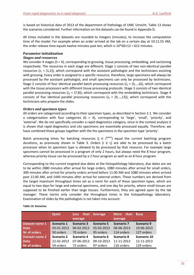
From rapid diagnostics to a rapid diagnosis A.G. Leeftink
35
is based on historical data of 2013 of the department of Pathology of UMC Utrecht. Table 13 shows the scenarios considered. Further information on the datasets can be found in Appendix D.
All times included in the datasets are rounded to integers (minutes), to increase the computation time of the model. For example when an order arrived at the lab on a certain day at 10:11:55 AM, the order release time equals twelve minutes past ten, which is 10*60+12 = 612 minutes.
Parameter initialization Stages and resources We consider 4 stages (S = 4), corresponding to grossing, tissue processing, embedding, and sectioning respectively. The resources in each stage are different. Stage 1 consists of two non-identical parallel resources (J1 = {1,2}), which correspond with the assistant pathologist and the technicians assisting with grossing. Every order is assigned to a specific resource, therefore, large specimens will always be processed by the assistant pathologist, and small specimens can only be processed by technicians. Stage 2 consists of four identical parallel batch processing resources (J2 = {3,…,6}), which correspond with the tissue processors with different tissue processing protocols. Stage 3 consists of two identical parallel processing resources (J3 = {7,8}), which correspond with the embedding technicians. Stage 4 consists of five identical parallel processing resources (J4 = {9,…,13}), which correspond with the technicians who prepare the slides.
Orders and specimen types All orders are categorized according to their specimen types, as described in Section 2.1. We consider a categorization with four categories (G = 4), corresponding to ‘large’, ‘small’, ‘priority’, and ‘external’. We do not specifically consider a rapid diagnostics category, since in the context analysis it is shown that rapid diagnostics and cito specimens are essentially processed equally. Therefore, we have combined these groups together with the htx specimens in the specimen type ‘priority’.
Batch processing times for batching resources (j ∈ Jbatch) equal the current batching program durations, as previously shown in Table 3. Orders (i ∈ Ij) are able to be processed by a batch processor when its specimen type is allowed to be processed by that resource. For example large specimens cannot be processed in a program of only 2 hours, but always need the 8 hour program, whereas priority tissue can be processed by a 2 hour program as well as an 8 hour program.
Corresponding to the current targeted due dates at the histopathology laboratory, due dates are set to be within 2880 minutes after arrival for large orders, 1080 minutes after arrival for small orders, 300 minutes after arrival for priority orders arrived before 11:00 AM and 1080 minutes when arrived past 11:00 AM, and 1440 minutes after arrival for external orders. These numbers are derived from the target maximum throughput times set as a norm for each of these specimen types, which are equal to two days for large and external specimens, and one day for priority, where small tissues are supposed to be finished earlier than large tissues. Furthermore, they are agreed upon by the lab manager. These norms only consider the throughput times in the histopathology laboratory. Examination of slides by the pathologists is not taken into account.
Table 13: Scenarios
Quiet Less than average
Average More than average
Busy
Dataset name 1 Date Nr of orders
Scenario 1 03-01-2013 50 orders
Scenario 3 06-02-2013 70 orders
Scenario 5 05-02-2013 95 orders
Scenario 7 06-06-2013 114 orders
Scenario 9 19-06-2013 127 orders
Dataset name 2 Date Nr of orders
Scenario 2 22-02-2013 59 orders
Scenario 4 07-06-2013 72 orders
Scenario 6 09-10-2013 97 orders
Scenario 8 11-11-2013 116 orders
Scenario 10 12-11-2013 129 orders
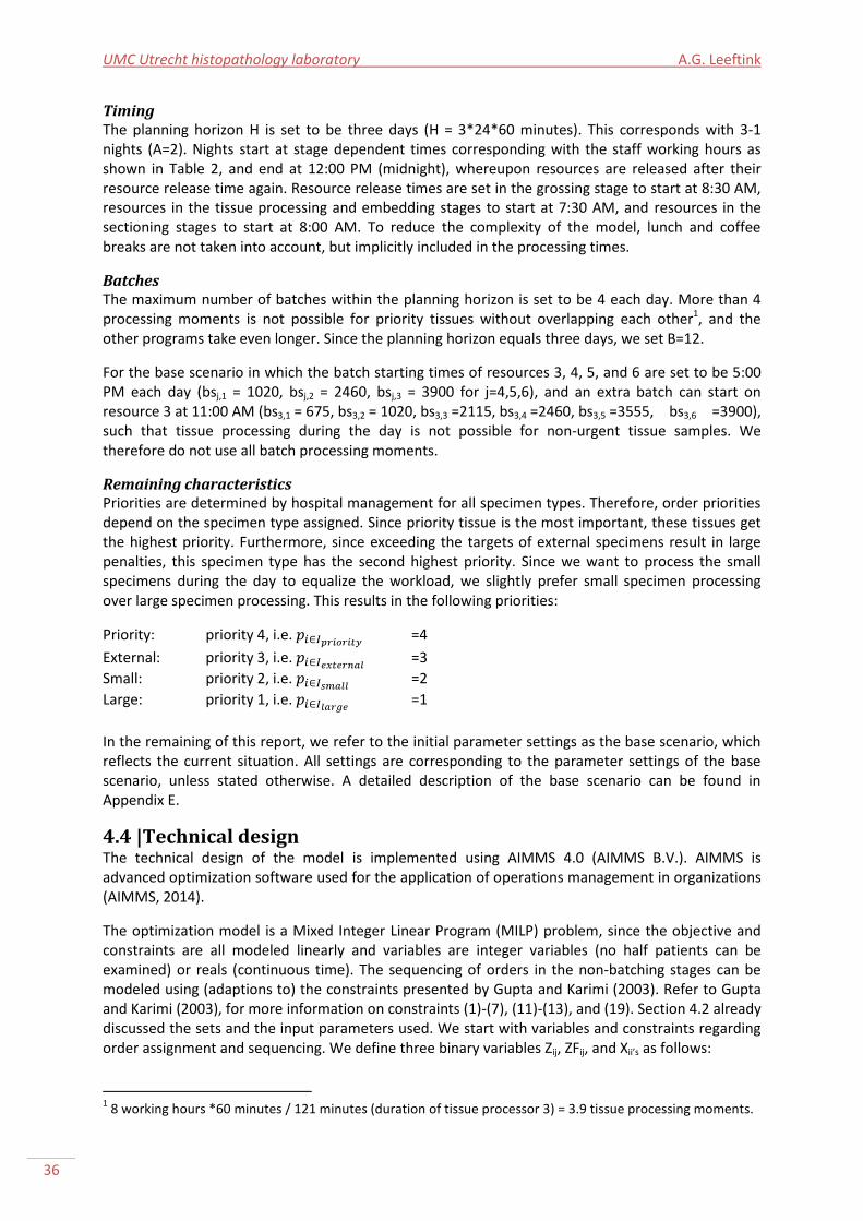
UMC Utrecht histopathology laboratory A.G. Leeftink
36
Timing The planning horizon H is set to be three days (H = 3*24*60 minutes). This corresponds with 3-1 nights (A=2). Nights start at stage dependent times corresponding with the staff working hours as shown in Table 2, and end at 12:00 PM (midnight), whereupon resources are released after their resource release time again. Resource release times are set in the grossing stage to start at 8:30 AM, resources in the tissue processing and embedding stages to start at 7:30 AM, and resources in the sectioning stages to start at 8:00 AM. To reduce the complexity of the model, lunch and coffee breaks are not taken into account, but implicitly included in the processing times.
Batches The maximum number of batches within the planning horizon is set to be 4 each day. More than 4 processing moments is not possible for priority tissues without overlapping each other1, and the other programs take even longer. Since the planning horizon equals three days, we set B=12.
For the base scenario in which the batch starting times of resources 3, 4, 5, and 6 are set to be 5:00 PM each day (bsj,1 = 1020, bsj,2 = 2460, bsj,3 = 3900 for j=4,5,6), and an extra batch can start on resource 3 at 11:00 AM (bs3,1 = 675, bs3,2 = 1020, bs3,3 =2115, bs3,4 =2460, bs3,5 =3555, bs3,6 =3900), such that tissue processing during the day is not possible for non-urgent tissue samples. We therefore do not use all batch processing moments.
Remaining characteristics Priorities are determined by hospital management for all specimen types. Therefore, order priorities depend on the specimen type assigned. Since priority tissue is the most important, these tissues get the highest priority. Furthermore, since exceeding the targets of external specimens result in large penalties, this specimen type has the second highest priority. Since we want to process the small specimens during the day to equalize the workload, we slightly prefer small specimen processing over large specimen processing. This results in the following priorities:
Priority: priority 4, i.e. =4
External: priority 3, i.e. =3
Small: priority 2, i.e. =2
Large: priority 1, i.e. =1
In the remaining of this report, we refer to the initial parameter settings as the base scenario, which reflects the current situation. All settings are corresponding to the parameter settings of the base scenario, unless stated otherwise. A detailed description of the base scenario can be found in Appendix E.
4.4 |Technical design The technical design of the model is implemented using AIMMS 4.0 (AIMMS B.V.). AIMMS is advanced optimization software used for the application of operations management in organizations (AIMMS, 2014).
The optimization model is a Mixed Integer Linear Program (MILP) problem, since the objective and constraints are all modeled linearly and variables are integer variables (no half patients can be examined) or reals (continuous time). The sequencing of orders in the non-batching stages can be modeled using (adaptions to) the constraints presented by Gupta and Karimi (2003). Refer to Gupta and Karimi (2003), for more information on constraints (1)-(7), (11)-(13), and (19). Section 4.2 already discussed the sets and the input parameters used. We start with variables and constraints regarding order assignment and sequencing. We define three binary variables Zij, ZFij, and Xii’s as follows:
1 8 working hours *60 minutes / 121 minutes (duration of tissue processor 3) = 3.9 tissue processing moments.
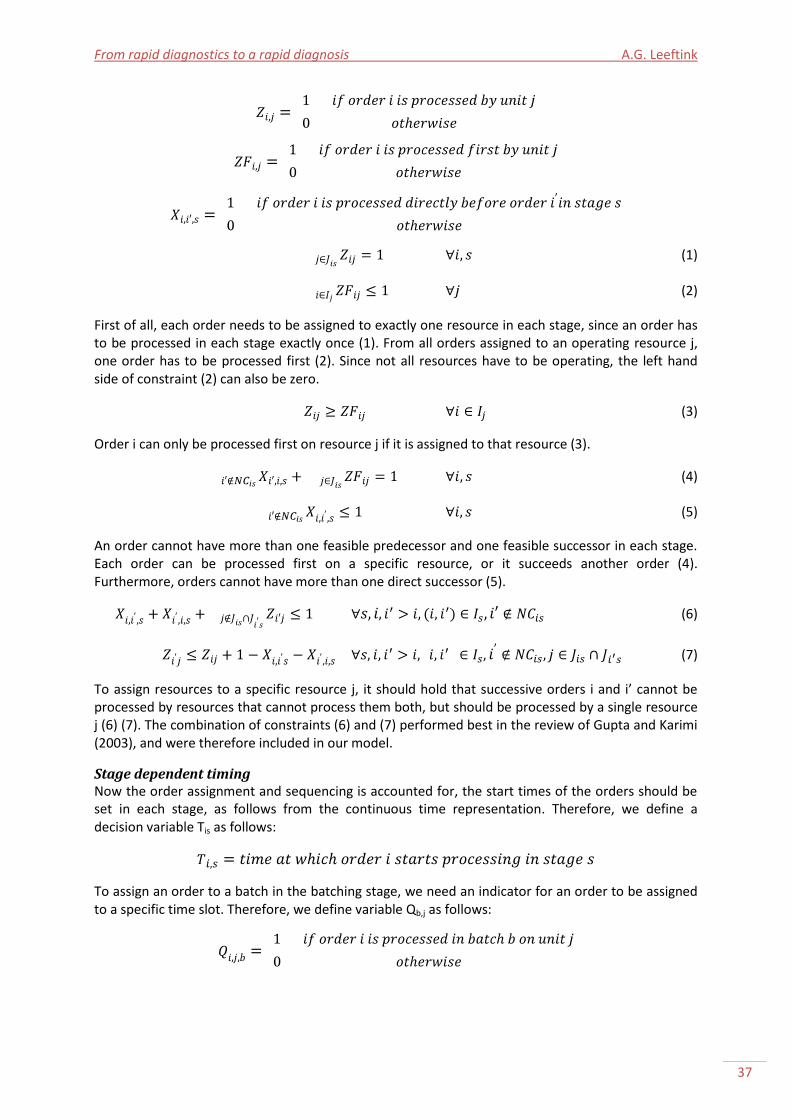
From rapid diagnostics to a rapid diagnosis A.G. Leeftink
37
(1)
(2)
First of all, each order needs to be assigned to exactly one resource in each stage, since an order has to be processed in each stage exactly once (1). From all orders assigned to an operating resource j, one order has to be processed first (2). Since not all resources have to be operating, the left hand side of constraint (2) can also be zero.
(3)
Order i can only be processed first on resource j if it is assigned to that resource (3).
(4)
(5)
An order cannot have more than one feasible predecessor and one feasible successor in each stage. Each order can be processed first on a specific resource, or it succeeds another order (4). Furthermore, orders cannot have more than one direct successor (5).
(6)
(7)
To assign resources to a specific resource j, it should hold that successive orders i and i’ cannot be processed by resources that cannot process them both, but should be processed by a single resource j (6) (7). The combination of constraints (6) and (7) performed best in the review of Gupta and Karimi (2003), and were therefore included in our model.
Stage dependent timing Now the order assignment and sequencing is accounted for, the start times of the orders should be set in each stage, as follows from the continuous time representation. Therefore, we define a decision variable Tis as follows:
To assign an order to a batch in the batching stage, we need an indicator for an order to be assigned to a specific time slot. Therefore, we define variable Qb,j as follows:

UMC Utrecht histopathology laboratory A.G. Leeftink
38
An order i can only start processing in the next stage, after order i has finished processing in the previous stage, and is transported to the next stage. Therefore, stage sequencing constraints are introduced.
(8)
When a batch b is selected in a batching stage, this batch should start processing after order i has finished processing in the previous stage, and is transported to the batching stage (8).
(9)
To start processing in a post-batch stage, all orders of the batch containing order i should be fully processed in the batching stage, and transported towards the post-batch stage (9), with nsis defined as the next processing stage of order i, currently being processed in stage s.
(10)
In the stage sequencing relation between two non-batching stages, order i has to finish processing in stage s and be transported to the next stage before starting in next stage (10). The stage dependent timing constraints are adapted from the timing constraint of Gupta and Karimi (2003) to take the increasing order size into account, and to correct for batching influences.
Order dependent timing Not only relations between stages influence the timing of orders on processing resources, also the relation between orders should be taken into account.
(11)
In all non-batching stages, order i’ can start processing on j after its predecessor order i is finished (11). This constraint is adapted from the constraint of Gupta and Karimi (2003) to take the increasing order size into account.
(12)
(13)
The timing of orders on resources is subject to some constraints. The first order i on resource j can only start processing after the release time of the resource (12). Furthermore, each order can only start processing after its release time (13). Setup times are not taken into account.
Batching The assignment of orders to a specific batch on a specific resource, is subject to two constraints.
(14)
All orders can only be assigned to one batch, which follows from constraint (14).
(15)
The corresponding batch starting time equals the order timing of order i in stage s (15).

From rapid diagnostics to a rapid diagnosis A.G. Leeftink
39
Night hours Orders can only start processing on resources when the resources are available. Since resources are unavailable during night-hours, we consider A nights during the planning horizon. To indicate if order i is planned before or after a certain night a, let Yais be an auxiliary binary variable defined as follows:
(16)
(17)
Processing of any order in any stage cannot start at moments it cannot be finished before the closing hours of the resource. Therefore, processing of an order i in stage s should start before or after the non-working moments (16) (17), which does not involve the transfer time. These constraints only holds for non-batching stages, since the batch processors in the histopathology laboratory model are able to work during night hours, when the process is started before the start of the night.
Objective The objective is to minimize the weighted tardiness of all orders. Let us define Tdi as follows:
(18)
The tardiness of order i equals the sum of the start time in last stage ( ), the transfer time of order i in this stage, and the order factor times the processing time of order i in this stage, which together equals the completion time of order i, minus the due date of order i (18). This constraint is adapted from Gupta and Karimi (2003).
(19)
Specific specimen types are more important to finish on time than others. Therefore, the orders are prioritized, by priority factor pi. This makes the objective to minimize the sum of the weighted tardiness (19).
Efficiency constraints Some additional constraints are proposed to make the MILP more efficient.
(20)
An upper bound on the order timing Tis can be given by the end time of the planning horizon H. A better upper bound is derived when subtracting the processing time of order i in the final stage. Since the processing times are equal in all resources, the last resource is chosen for the upper bound determination. This results in constraint (20).
(21)
When an order cannot be processed by resource j, since it is not allowed to be processed by that
resource (i.e. ), the order cannot be assigned to that resource (21).
To indicate whether a resource is working, let us define binary variable UWj as follows:
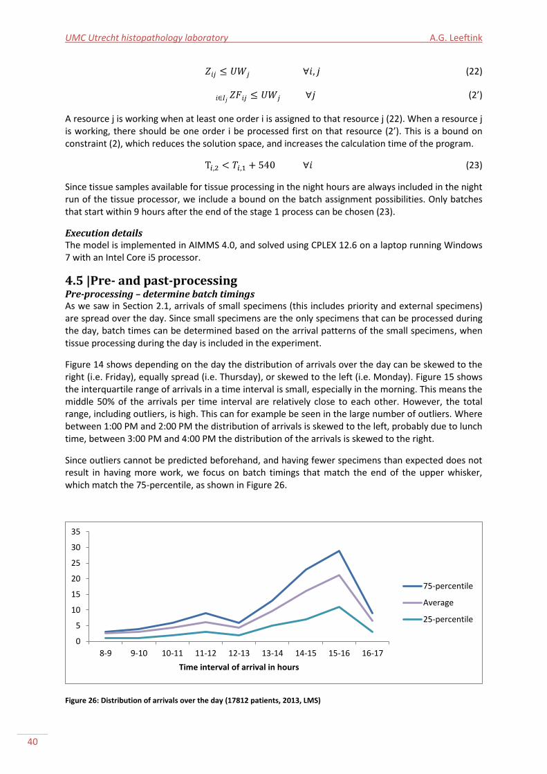
UMC Utrecht histopathology laboratory A.G. Leeftink
40
(22)
(2’)
A resource j is working when at least one order i is assigned to that resource j (22). When a resource j is working, there should be one order i be processed first on that resource (2’). This is a bound on constraint (2), which reduces the solution space, and increases the calculation time of the program.
(23)
Since tissue samples available for tissue processing in the night hours are always included in the night run of the tissue processor, we include a bound on the batch assignment possibilities. Only batches that start within 9 hours after the end of the stage 1 process can be chosen (23).
Execution details The model is implemented in AIMMS 4.0, and solved using CPLEX 12.6 on a laptop running Windows 7 with an Intel Core i5 processor.
4.5 |Pre- and past-processing Pre-processing – determine batch timings As we saw in Section 2.1, arrivals of small specimens (this includes priority and external specimens) are spread over the day. Since small specimens are the only specimens that can be processed during the day, batch times can be determined based on the arrival patterns of the small specimens, when tissue processing during the day is included in the experiment.
Figure 14 shows depending on the day the distribution of arrivals over the day can be skewed to the right (i.e. Friday), equally spread (i.e. Thursday), or skewed to the left (i.e. Monday). Figure 15 shows the interquartile range of arrivals in a time interval is small, especially in the morning. This means the middle 50% of the arrivals per time interval are relatively close to each other. However, the total range, including outliers, is high. This can for example be seen in the large number of outliers. Where between 1:00 PM and 2:00 PM the distribution of arrivals is skewed to the left, probably due to lunch time, between 3:00 PM and 4:00 PM the distribution of the arrivals is skewed to the right.
Since outliers cannot be predicted beforehand, and having fewer specimens than expected does not result in having more work, we focus on batch timings that match the end of the upper whisker, which match the 75-percentile, as shown in Figure 26.
Figure 26: Distribution of arrivals over the day (17812 patients, 2013, LMS)
0
5
10
15
20
25
30
35
8-9 9-10 10-11 11-12 12-13 13-14 14-15 15-16 16-17
Time interval of arrival in hours
75-percentile
Average
25-percentile
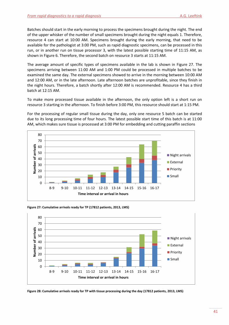
From rapid diagnostics to a rapid diagnosis A.G. Leeftink
41
Batches should start in the early morning to process the specimens brought during the night. The end of the upper whisker of the number of small specimens brought during the night equals 1. Therefore, resource 4 can start at 10:00 AM. Specimens brought during the early morning, that need to be available for the pathologist at 3:00 PM, such as rapid diagnostic specimens, can be processed in this run, or in another run on tissue processor 3, with the latest possible starting time of 11:15 AM, as shown in Figure 6. Therefore, the second batch on resource 3 starts at 11:15 AM.
The average amount of specific types of specimens available in the lab is shown in Figure 27. The specimens arriving between 11:00 AM and 1:00 PM could be processed in multiple batches to be examined the same day. The external specimens showed to arrive in the morning between 10:00 AM and 12:00 AM, or in the late afternoon. Late afternoon batches are unprofitable, since they finish in the night hours. Therefore, a batch shortly after 12:00 AM is recommended. Resource 4 has a third batch at 12:15 AM.
To make more processed tissue available in the afternoon, the only option left is a short run on resource 3 starting in the afternoon. To finish before 3:00 PM, this resource should start at 1:15 PM.
For the processing of regular small tissue during the day, only one resource 5 batch can be started due to its long processing time of four hours. The latest possible start time of this batch is at 11:00 AM, which makes sure tissue is processed at 3:00 PM for embedding and cutting paraffin sections
Figure 27: Cumulative arrivals ready for TP (17812 patients, 2013, LMS)
Figure 28: Cumulative arrivals ready for TP with tissue processing during the day (17812 patients, 2013, LMS)
0
10
20
30
40
50
60
70
80
8-9 9-10 10-11 11-12 12-13 13-14 14-15 15-16 16-17
Nu
mb
er
of
arri
vals
Time interval or arrival in hours
Night arrivals
External
Priority
Small
0
10
20
30
40
50
60
70
80
8-9 9-10 10-11 11-12 12-13 13-14 14-15 15-16 16-17
Nu
mb
er
of
arri
vals
Time interval or arrival in hours
Night arrivals
External
Priority
Small

UMC Utrecht histopathology laboratory A.G. Leeftink
42
purposes. This leaves two hours for embedding, cutting paraffin sections, and staining of all those tissues, which is in compliance with the 75-percentile of arrivals (7 arrivals, which take 60 minutes2 of further processing and 60 minutes of staining each).
The expected impact of these processing moments can be seen by comparing Figure 27 with Figure 28. As seen, fewer specimens are stored at the patient administration during the day, and fewer specimens are loaded in the night run. This enables the technicians to anticipate on the large bulk of specimens arriving between 2:00 PM and 4:00 PM.
Due to these bulk arrivals, further optimization of the batch starting times by the use of exact and/or approximate approaches is not taken into account, since the processing of specimens arriving in that time interval cannot be done during the day.
Concluding, for the tissue processing during the day scenario, the batch starting times of resources 3, 4, 5, and 6 (bsjb) are set to be equal to the latest opening times each day (i.e. 5:00 PM, or 5:30 PM). Furthermore, extra batches are determined to start on resource 3 at 11:15 AM and 1:15 PM, on resource 4 at 10:00 AM and 12:15 AM, and on resource 5 at 11:00 AM.
Past-processing - practicability constraints Even though a solution is optimal, the implementation in practice can turn out to fail because of practical reasons. Therefore, after an (optimal) solution is derived, we execute a past processing algorithm, as shown in Appendix F. This algorithm uses the sequence of the (optimal) solution, and schedules all orders in that sequence on the assigned resources at the earliest possible time. This increases the practicability since technicians want to start working on the next order if this order is already available in their stage, even if it can wait for (for example) 10 more minutes. Furthermore, the algorithm does not negatively influence the solution quality, since orders cannot be scheduled later than scheduled in the solution obtained from the MILP model.
4.6 |Verification “Verification is concerned with determining whether the assumptions have been correctly translated into a computer program” (Law, 2007, pp 243). Multiple techniques are available to validate a program, which involve debugging the model, reviewing the model with more than one person, and checking the output of the model under a variety of input parameter settings (Law, 2007).
We verified the model based on these techniques. First of all, the model should give output without any bugs. Since the model runs for small as well as large datasets, the model is valid to this point. Second, the model is developed and reviewed not only by people from the University of Twente, which have a mathematical background, but also by people from the hospital, which have a medical background. Therefore, we consider the model verified to this point. Third, the model is run with a small (10 orders) dataset to see if the output matches the expected output. In these cases, the output of the model proved to be optimal. For larger datasets the output seemed reasonable, and no further improvements could be made by hand, which suggest the output to be (close to) optimal. Concluding, the model is verified based on the techniques described.
4.7 |Conclusions In this chapter, a verified MILP-model is developed, with input and output as schematically displayed in Figure 29. The model assigns orders to a processing resource in each stage, it sequences the orders on each resource, and it determines the processing start times of all orders in each stage on each resource. The output of the model is a schedule of all orders for each resource in use. From this schedule, the workload per resource, the start and end processing times per order, the batch sizes of the batch processing resources, and the performance of the system in terms of throughput time per
2 6,2 cassettes * 2 minutes embedding and 11,9 slides * 4 minutes cutting paraffin sections = 60 minutes.
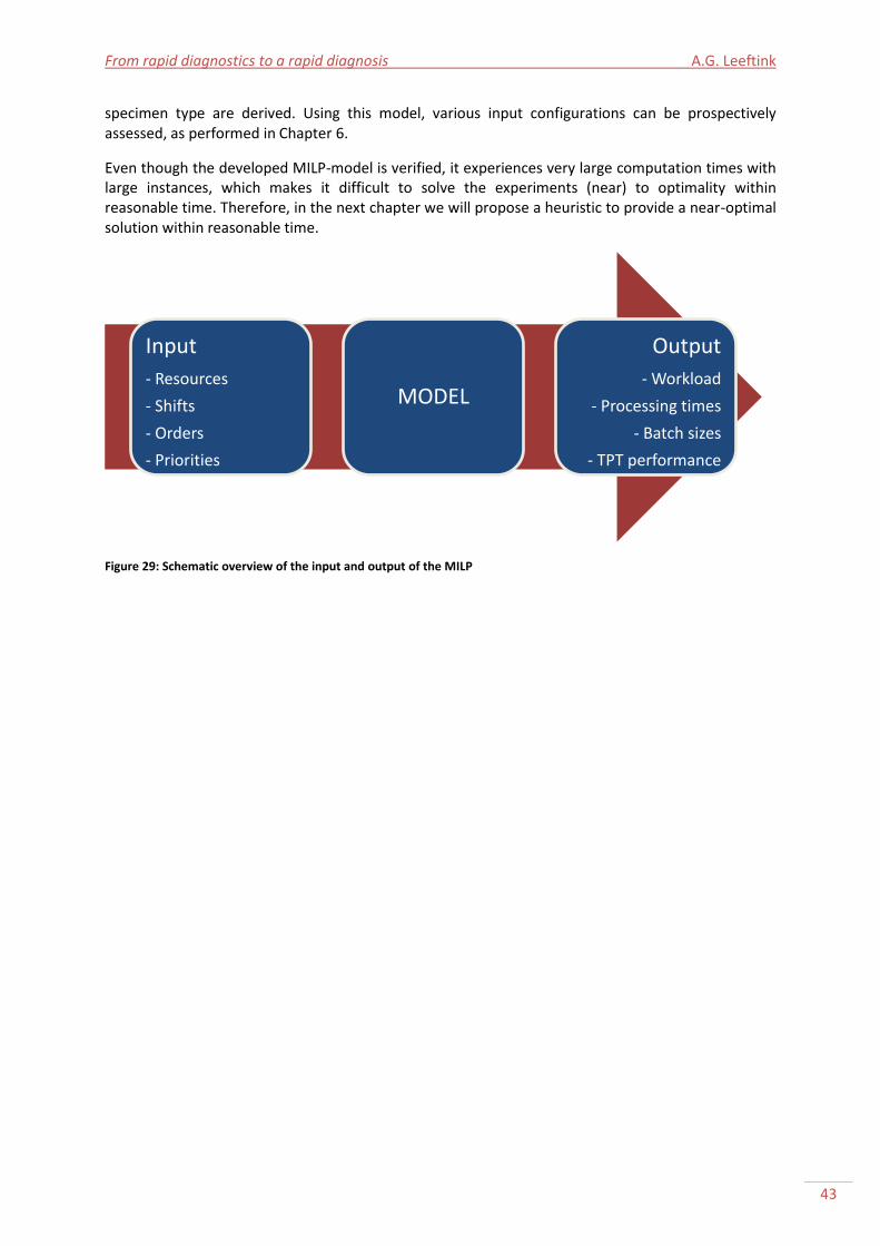
From rapid diagnostics to a rapid diagnosis A.G. Leeftink
43
specimen type are derived. Using this model, various input configurations can be prospectively assessed, as performed in Chapter 6.
Even though the developed MILP-model is verified, it experiences very large computation times with large instances, which makes it difficult to solve the experiments (near) to optimality within reasonable time. Therefore, in the next chapter we will propose a heuristic to provide a near-optimal solution within reasonable time.
Figure 29: Schematic overview of the input and output of the MILP
Input
- Resources
- Shifts
- Orders
- Priorities
MODEL
Output
- Workload
- Processing times
- Batch sizes
- TPT performance

UMC Utrecht histopathology laboratory A.G. Leeftink
44
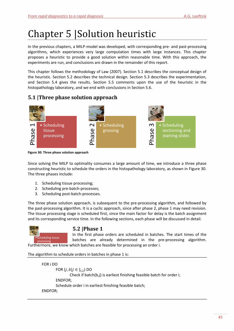
From rapid diagnostics to a rapid diagnosis A.G. Leeftink
45
Ph
ase
1
• Scheduling tissue processing
Ph
ase
2
• Scheduling grossing
Ph
ase
3
• Scheduling sectioning and staining slides
•Scheduling tissue processing
Chapter 5 |Solution heuristic In the previous chapters, a MILP-model was developed, with corresponding pre- and past-processing algorithms, which experiences very large computation times with large instances. This chapter proposes a heuristic to provide a good solution within reasonable time. With this approach, the experiments are run, and conclusions are drawn in the remainder of this report.
This chapter follows the methodology of Law (2007). Section 5.1 describes the conceptual design of the heuristic. Section 5.2 describes the technical design. Section 5.3 describes the experimentation, and Section 5.4 gives the results. Section 5.5 comments upon the use of the heuristic in the histopathology laboratory, and we end with conclusions in Section 5.6.
5.1 |Three phase solution approach
Since solving the MILP to optimality consumes a large amount of time, we introduce a three phase constructing heuristic to schedule the orders in the histopathology laboratory, as shown in Figure 30. The three phases include:
1. Scheduling tissue processing; 2. Scheduling pre-batch-processes; 3. Scheduling post-batch-processes.
The three phase solution approach, is subsequent to the pre-processing algorithm, and followed by the past-processing algorithm. It is a cyclic approach, since after phase 2, phase 1 may need revision. The tissue processing stage is scheduled first, since the main factor for delay is the batch assignment and its corresponding service time. In the following sections, each phase will be discussed in detail.
5.2 |Phase 1 In the first phase orders are scheduled in batches. The start times of the batches are already determined in the pre-processing algorithm.
Furthermore, we know which batches are feasible for processing an order i.
The algorithm to schedule orders in batches in phase 1 is:
FOR i DO FOR ( ) DO Check if batch(b,j) is earliest finishing feasible batch for order i; ENDFOR; Schedule order i in earliest finishing feasible batch; ENDFOR;
Figure 30: Three phase solution approach
UMC Utrecht histopathology laboratory A.G. Leeftink
46
•Scheduling grossing
In this algorithm, all orders i are scheduled in a batch b on resource j that is feasible. For each order, the earliest finishing batch out of its pool of feasible batches is chosen, and the order is scheduled in this batch. Since the capacity of all batches is assumed unlimited, the scheduling of an order in a batch does not influence the processing times of the remaining orders. If all orders are scheduled in their earliest finishing feasible batch, the final solution will be the optimal solution, since finishing earlier is not possible. A batch is feasible when the batch starts after the order release time, and when the batch is feasible for the specimen type of the order on hand. This way, the throughput time over stage 1 and 2 of order i is minimized.
5.3 |Phase 2 In phase 2 the grossing activities of stage 1 scheduled, given the order assignment to a batch in stage 2. A distinction has to be made for large
specimens, and the remaining specimens, since large specimens are the only specimens allowed to be grossed by a resident (resource 1), and the remaining specimens are grossed by a technician (resource 2).
Phase 2 - Large Large specimens arrive in the histopathology laboratory in large batches, due to the need for overnight fixation. Since large specimens can only be processed in night runs of the tissue processor, these specimens need to be grossed during the day, and all orders are in the same batch. To reduce the delay, the specimens can be scheduled following the FIFO principle (First In First Out), or the EDD principle (Earliest Due Date), since the due dates of the large specimens equal the time of arrival added with a standard time interval.
The algorithm to schedule orders of specimen type large on resource 1 is:
Sort i on earliest due date; FOR i DO
Schedule i; IF i scheduled within [NW1a1, NW2a + URT1] THEN
Reschedule i after night hours; ENDIF;
Check batch starting time; ENDFOR;
In this algorithm, all orders i are scheduled in a row, after being sorted on earliest due date. The order with the first due date is scheduled at the earliest possible time, the second due order is scheduled when the first due order is finished, etcetera.
When the shift of the resident is ended, the next orders are scheduled starting from the next day. If this happens, the assignment to a batch of the remaining orders has to be rescheduled, since their current batch is not feasible anymore.
Phase 2 - Remaining The scheduling of the remaining tissues (e.g. small, external, and priority) on resource 2 is more complex. These orders have different due dates and arrival times. For example: A priority tissue that arrives later than a small tissue can be due earlier. Now we know the batch times of the orders, we can schedule per time unit the orders on earliest batch time first, and within these batches on earliest due date, such that postponement of early due orders is reduced.
From rapid diagnostics to a rapid diagnosis A.G. Leeftink
47
•Scheduling sectioning and staining slides
The algorithm to schedule orders of the remaining specimen types on resource 2 is:
Time := Release time resource 2 WHILE time < horizon DO FOR batches DO //earliest batch first Find feasible order in batch with EDD;
ENDFOR; IF order found THEN Check feasibility with batch starting time;
IF batch starting time is feasible THEN Schedule i on time; Time := Time + processing time i; ELSE Reschedule batch (Phase 1);
ENDIF; ELSE
Time := Time + 1; ENDIF; ENDWHILE;
In this algorithm, the orders within a batch are scheduled based on their earliest due date. The order with the earliest due date, which is feasible in terms of arrival time, is evaluated on the batch starting time. If the timing fits, the order is scheduled, and the next order is scheduled after finishing this order. If not, the batch is rescheduled.
By rescheduling batches, the solution will lose its guarantee of optimality. However, since only those orders with a late due date are rescheduled, we assume the solution will be, although not optimal, a good solution.
5.4 |Phase 3 In phase 3 orders are scheduled on the remaining resources of stage 3 and 4. This can be performed using the MILP model developed in Chapter 4, or using
a heuristic approach.
MILP When solving the stage 3 and 4 scheduling problem using the MILP model, we restrict the resources in the model to the resources of stage 3 and 4, and remove the batching constraints. The order release time to stage 3 equals to the finish time of the batches they are scheduled in.
The algorithm to schedule orders in stage 3 and 4 is:
Solve MILP;
In this algorithm, the Mixed Integer Linear Program of Chapter 4 is executed for stage 3 and 4 (s = 3,4), with resources 6 to 13 (j = 6, .., 13), only. The MILP will schedule orders on these resources in these stages. Since the batching constraints have been eliminated, and two stages and six resources are removed, the complexity of the problem is severely reduced, which will positively influence the calculation time.
Heuristic approach When solving the stage 3 and 4 scheduling problem using a heuristic approach, we can schedule the orders based on earliest due date, corresponding to the approach used in Phase 2. However, now the due date of the orders corresponds to the final due date of the order.
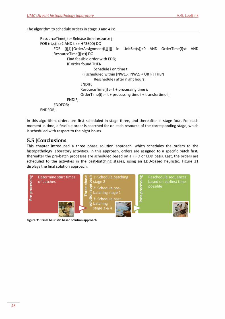
UMC Utrecht histopathology laboratory A.G. Leeftink
48
The algorithm to schedule orders in stage 3 and 4 is:
ResourceTime(j) := Release time resource j FOR ((t,s)|s>2 AND t <= H*3600) DO
FOR ((j,i)|OrderAssignment(i,jj|jj in UnitSet(s))=0 AND OrderTime(i)<t AND ResourceTime(j)<t)) DO
Find feasible order with EDD; IF order found THEN Schedule i on time t; IF i scheduled within [NW1a1, NW2a + URT1] THEN
Reschedule i after night hours; ENDIF; ResourceTime(j) := t + processing time i; OrderTime(i) := t + processing time i + transfertime i; ENDIF; ENDFOR;
ENDFOR;
In this algorithm, orders are first scheduled in stage three, and thereafter in stage four. For each moment in time, a feasible order is searched for on each resource of the corresponding stage, which is scheduled with respect to the night hours.
5.5 |Conclusions This chapter introduced a three phase solution approach, which schedules the orders to the histopathology laboratory activities. In this approach, orders are assigned to a specific batch first, thereafter the pre-batch processes are scheduled based on a FIFO or EDD basis. Last, the orders are scheduled to the activities in the past-batching stages, using an EDD-based heuristic. Figure 31 displays the final solution approach.
Figure 31: Final heuristic based solution approach
Pre
-pro
cess
ing Determine start times
of batches
Thre
e p
has
e
solu
tio
n a
pp
roac
h
1: Schedule batching stage 2
2: Schedule pre-batching stage 1
3: Schedule past-batching stage 3 & 4
Pas
t-p
roce
ssin
g Reschedule sequences based on earliest time possible

From rapid diagnostics to a rapid diagnosis A.G. Leeftink
49
Chapter 6 |Computational results This chapter validates the model (Section 6.1) and evaluates the experiment design (Section 6.2). Then, outcomes are given (Section 6.3) and evaluated (Section 6.4). Some limitations of the model are described in Section 6.5. Finally, a conclusion is given in Section 6.6, which provides an answer to the 5th research question regarding the computational effects of the selected interventions.
6.1 |Validation A valid model is an accurate representation of the actual system under consideration. When a model is valid, the model can be used to make decisions based on experiments as if they were experimented on the actual system. Validation is the process of determining if the model does represent the actual situation, for the objectives of the study (Law, 2007).
One approach for validation is to apply sensitivity analysis, in which parameter values, entities, level of detail and the data are evaluated (Law, 2007). However, due to time constraints we do not include this in this research. The most definitive validation test is to compare the output of the model with the output of the actual system under consideration (Law, 2007). In this study, the validation is conducted by comparing the performance of both the modeled and the actual system, based on the performance indicators, and also by a review of the technicians, lab manager, and pathologists to see if model outcomes of the base scenario reflect reality.
We assume the model to be valid when the average of the performance of the fifth and sixth dataset on the base scenario, which have an average number of arrivals, is in compliance with the current performance, i.e. the performance on the performance indicators determined in Chapter 2: Percentage of specimens on time and the workload. Since the data in these datasets are based on historical data, we can match the outcome of the model with the real performance of the orders modeled.
Table 14 shows the output derived on the performance indicators, for the base scenario in which the batch starting times of resources 3, 4, 5, and 6 are set to be 5:00 PM, and an extra batch can start on resource 3 at 11:15 AM, such that tissue processing during the day is not possible for non-urgent tissue samples. The performance of the fifth and sixth intervention is shown in the first columns. The average percentages of the model are given, as well as the performance of the actual system, as described in Chapter 2, which is shown by the average percentages in theory. The difference (Δ) between these two performances is given, and it is indicated if this difference can be occurred by change, or is a significant difference.
Table 14: Base scenario performance for validation, with df=1, p<0,05 (22379 patients, 2013, LMS & U-DPS)
Dataset 5 6 Avg model Avg theory Δ Difference significant?
% large in 4 days 100% 85% 92.5% 79% 13,5% Significant (p>0,05)
% small in 2 days 74% 74% 74% 73% 1,0% Not significant (p<0,05)
% priority in 1 day 100% 100% 100% 64% 36,0% -3
% external in 2 days 100% 97% 98.5% 89% 9,5% Significant (p>0,05)
Delta workload 10.5% 12.4% 11.5% 9.6% 1,9% -4
3 The expected number of observations not examined on time is lower than 5, which makes a chi-squared
statistical test an unreliable measure, and therefore inapplicable. 4 No distribution is available.
UMC Utrecht histopathology laboratory A.G. Leeftink
50
The percentages of specimens examined on time for small specimens show no significant differences in actual and theoretical performance. However, the other three throughput time performance measures show a significant difference, or have too few observations to apply a chi-square statistical test to. More information on the application of the chi-square tests can be found in Appendix I.
Comparing the actual performance with the modeled performance, the difference is especially large in the percentages on time for priority specimens: a 36% difference. Furthermore, no statistical test can be applied to this performance, since the expected unsuccessful observations are too small. We already mentioned earlier that the theoretical priority TPT performance measured is unreliable, since in 2013, all MDM meetings have been attended. This is in compliance with the modeled performance, since 100% of the deadlines are met, which means all MDM meetings were attended.
The difference in TPT performance of the large specimens can be explained by the fact that the model does not include casualties, extra fixation needed, and unnecessary waiting. The difference in TPT performance of the external specimens can be due to the different TPT norm measures that are used in practice, since it is a compounded performance measure of private clinics and general practitioners, which have more strict deadlines. For these reasons, we choose to accept these performance flaws.
Furthermore, the small difference of less than 2% in delta workload we regard as valid.
The most important validation activity is the discussion of the model with department of Pathology staff. In a review by important stakeholders of the department of Pathology, as mentioned above, the model´s input and output is said to be consistent with the perceived performance of the system. Therefore, we consider the model as face valid (Law, 2007).
Even though the modeled output is not significant for all specimen types, we think the model can still give some valuable insights in the performance of the histopathology laboratory. Furthermore, the stakeholders reviewed the output and its visual representation as a reliable reflection of reality. Therefore, we assume the model to be an accurate representation of the actual situation, and we assume the model to be face valid.
6.2 |Experiment design In this section, experiments are designed to evaluate the system’s performance under different circumstances. In several interventions, we will change some parameter settings, to evaluate the impact on the output of the system. All unchanged settings are corresponding to the parameter settings as explained in the base scenario in Section 4.3, unless stated otherwise.
Based on the interventions selected in Chapter 3, interventions in which different staffing configurations, such as extended working hours, staggered working hours, and schedules adapted to the pathologists’ agendas were selected. Furthermore, different starting times of batches are evaluated. The final selection of 9 interventions has been made in cooperation with the technicians, pathologists, head of the department of Pathology, and lab manager. Refer to Table 15 for an overview of the interventions selected.
During the experiments, we test all interventions on all scenarios developed in Section 4.3. In total we perform 9*10=90 experiments. The performance of all experiments is evaluated based on the performance indicators determined in Chapter 2.
Increasing the problem size, the computation time of the MILP in phase 3 can become severe. Therefore, we only allow the model to calculate up to 1 hour (3600 seconds). If this time limit is exceeded, the computation will be interrupted, and the solution will be evaluated taking the integrality gap into account.
From rapid diagnostics to a rapid diagnosis A.G. Leeftink
51
N/D. Batching moments on tissue processor We consider two types of tissue processing configurations: interventions with the regular tissue processing configurations (only priority samples are processed during the day, indicated with an N (night)) and interventions in which tissue processing during the day is facilitated (indicated with a D (day)). This last intervention type consists of the model without the restriction on tissue processing during the day for non-urgent tissues. The evaluation of these interventions will give insight in the effect of tissue processing during the day, and the consequences of this rule for the performance of the histopathology laboratory.
The different configurations for the batching times are evaluated in the preprocessing algorithm.
1. Current situation (base scenario + night processing constraint) In the current situation consists of the base scenario parameter settings as explained in Section 4.3. This situation is based on the order data of 2013, and resource data as used by the histopathology laboratory for scheduling in May 2014. The settings represent the current situation in the histopathology laboratory, where tissue processing during the day is only possible for priority tissues.
2. Extended working hours
A – Resident small earlier and technicians later When aiming for tissue processing during the day, it intuitively is interesting to see the effect of an earlier starting time of the resident/technician who grosses the small specimens. This hypothetically causes the small tissues to be grossed earlier, which creates the opportunity to process them in a tissue processing run during the day. Therefore, intervention 2A adapts the working hours of resource 2 to be starting one hour earlier.
Furthermore, a higher availability of technicians in the afternoon could facilitate slide preparation after tissue processing in the afternoon. Since this intervention is designed for tissue processing during the day, we only test the day-variant, and exclude the night-variant from the experiments.
B – Technicians earlier To increase the amount of slides ready for examination before the 1:00 PM deadline, the technicians could start working earlier. However, when aiming for tissue processing during the day, at least one embedding technician and one cutting technician should be available in the afternoon for urgent specimens. All technicians starting early is therefore not possible and staggering shifts is needed. Since this intervention is designed for improving the current processing configurations, we only test the night-variant, and exclude the day-variant from the experiments.
C – Technicians earlier and later and resident small earlier Adding the earlier starting time of the resident small to the previous situation, the earlier starting time of the small grossing could increase the throughput time of these specimens. Since this intervention is designed for tissue processing during the day, we only test the day-variant, and exclude the night-variant from the experiments.
D – Staggered shifts If the opening and closing times of the lab are the same as they currently are, the shifts can still be more staggered. To see if this makes any difference in throughput time and workload, this intervention is evaluated.
3. Pathologists agenda To evaluate a situation in which lean is fully adapted, we should consider a pull situation in which the laboratory is fully adapted to the pathologists agendas. Currently, it is said that pathologists need the slides to be ready at 1:00 PM, to be evaluated the same day. To facilitate this, the working hours were calculated to comply with this pull situation, as shown in Appendix G.
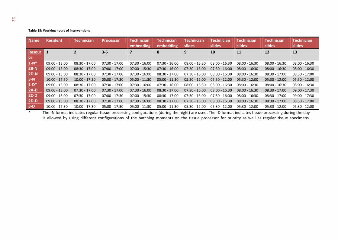
52
Table 15: Working hours of interventions
Name Resident Technician Processor Technician embedding
Technician embedding
Technician slides
Technician slides
Technician slides
Technician slides
Technician slides
Resource
1 2 3-6 7 8 9 10 11 12 13
1-N* 09:00 - 13:00 08:30 - 17:00 07:30 - 17:00 07:30 - 16:00 07:30 - 16:00 08:00 - 16:30 08:00 - 16:30 08:00 - 16:30 08:00 - 16:30 08:00 - 16:30
2B-N 09:00 - 13:00 08:30 - 17:00 07:00 - 17:00 07:00 - 15:30 07:30 - 16:00 07:30 - 16:00 07:30 - 16:00 08:00 - 16:30 08:00 - 16:30 08:00 - 16:30
2D-N 09:00 - 13:00 08:30 - 17:00 07:30 - 17:00 07:30 - 16:00 08:30 - 17:00 07:30 - 16:00 08:00 - 16:30 08:00 - 16:30 08:30 - 17:00 08:30 - 17:00
3-N 10:00 - 17:30 10:00 - 17:30 05:00 - 17:30 05:00 - 11:30 05:00 - 11:30 05:30 - 12:00 05:30 - 12:00 05:30 - 12:00 05:30 - 12:00 05:30 - 12:00
1-D* 09:00 - 13:00 08:30 - 17:00 07:30 - 17:00 07:30 - 16:00 07:30 - 16:00 08:00 - 16:30 08:00 - 16:30 08:00 - 16:30 08:00 - 16:30 08:00 - 16:30
2A-D 09:00 - 13:00 07:30 - 17:00 07:30 - 17:00 07:30 - 16:00 08:30 - 17:00 07:30 - 16:00 08:00 - 16:30 08:00 - 16:30 08:30 - 17:00 09:00 - 17:30
2C-D 09:00 - 13:00 07:30 - 17:00 07:00 - 17:30 07:00 - 15:30 08:30 - 17:00 07:30 - 16:00 07:30 - 16:00 08:00 - 16:30 08:30 - 17:00 09:00 - 17:30
2D-D 09:00 - 13:00 08:30 - 17:00 07:30 - 17:00 07:30 - 16:00 08:30 - 17:00 07:30 - 16:00 08:00 - 16:30 08:00 - 16:30 08:30 - 17:00 08:30 - 17:00
3-D 10:00 - 17:30 10:00 - 17:30 05:00 - 17:30 05:00 - 11:30 05:00 - 11:30 05:30 - 12:00 05:30 - 12:00 05:30 - 12:00 05:30 - 12:00 05:30 - 12:00
* The -N format indicates regular tissue processing configurations (during the night) are used. The -D format indicates tissue processing during the day is allowed by using different configurations of the batching moments on the tissue processor for priority as well as regular tissue specimens.

53
Table 16: Performance of heuristic-based experiments: % of specimens on time per specimen type, TPT2 in hours, and delta workload
Intervention
1-N 2B-N 2D-N 3-N 1-D 2A-D 2C-D 2D-D 3-D
Dat
ase
t
1 % large % small % priority % external TPT2 Delta workload
100 96 100 100 26.49 12.5 (m) 5
100 96 100 100 26.25 10.3 (m)
100 96 100 100 26.67 14.3 (m)
100 100 95 100 23.89 19.1 (a)
100 100 95 100 24.91 10.8 (m)
100 100 95 100 25.38 11.5 (m)
100 100 95 100 25.32 10.5 (m)
100 100 95 100 24.85 11.9 (m)
100 100 95 100 24.10 18.0 (a)
2 % large % small % priority % external TPT2 Delta workload
95 60 94 100 27.60 10.4 (m)
91 57 100 100 27.69 8.2 (m)
91 87 100 100 27.30 10.7 (m)
100 100 94 100 24.29 23.5 (a)
95 100 94 100 25.68 8.4 (m)
91 100 88 100 24.38 8.1 (m)
91 100 94 100 26.12 7.7 (m)
91 100 94 100 25.73 9.1 (m)
100 100 94 100 24.17 21.4 (a)
3 % large % small % priority % external TPT2 Delta workload
93 88 100 100 25.44 4.8 (m)
87 91 100 100 25.14 2.1 (m)
87 85 100 95 25.75 6.4 (m)
100 100 88 100 22.56 25.9 (a)
100 100 100 100 21.71 0.2 (a)
93 100 100 100 22.72 2.2 (m)
93 100 100 100 22.00 1.0 (a)
93 100 100 100 22.52 1.6 (m)
100 100 88 100 22.43 24.9 (a)
4 % large % small % priority % external TPT2 Delta workload
100 59 100 90 24.59 6.3 (m)
100 46 100 90 24.63 4.5 (m)
100 51 100 90 24.88 8.5 (m)
100 85 100 100 20.88 23.5 (a)
100 100 100 100 17.44 2.9 (a)
100 100 100 100 17.80 2.4 (a)
100 100 100 100 18.38 3.4 (a)
100 87 100 100 19.03 0.2 (m)
100 59 100 100 21.26 21.2 (a)
5 % large % small % priority % external
100 74 100 100
91 41 100 100
87 59 100 100
100 72 60 100
96 100 60 100
91 100 60 100
91 100 60 100
91 100 60 100
100 100 60 100
5 (m) indicates the workload is larger in the morning, (a) indicates the workload is larger in the afternoon

54
TPT2 Delta workload
26.48 10.5 (m)
26.76 8.9 (m)
27.06 12.2 (m)
24.05 23.1 (a)
22.54 3.7 (m)
22.89 4.9 (m)
21.77 4.8 (m)
23.13 4.8 (m)
23.86 22.3 (a)
6 % large % small % priority % external TPT2 Delta workload
85 74 100 97 24.95 12.4 (m)
90 67 100 97 24.80 10.2 (m)
86 77 100 97 25.00 13.7 (m)
100 100 80 100 21.88 21.8 (a)
95 100 100 100 19.40 4.2 (m)
90 100 100 100 19.74 5.2 (m)
95 100 100 100 19.78 4.9 (m)
90 100 100 100 20.56 7.4 (m)
100 100 80 100 21.80 20.5 (a)
7 % large % small % priority % external TPT2 Delta workload
83 20 100 60 25.47 12.6 (m)
88 33 100 56 24.25 9.8 (m)
88 19 100 67 24.85 13.6 (m)
100 63 100 100 20.33 19.7 (a)
100 91 100 100 15.53 0.7 (a)
94 98 100 100 15.85 2.8 (m)
94 100 100 100 16.43 0.5 (m)
94 95 100 100 15.86 4.0 (m)
100 70 100 100 20.28 19.0 (a)
8 % large % small % priority % external TPT2 Delta workload
82 28 94 46 25.19 13.2 (m)
79 30 94 35 25.28 11.6 (m)
79 38 94 38 25.75 15.0 (m)
100 55 82 100 21.56 18.0 (a)
79 65 100 100 19.06 7.1 (m)
79 78 88 100 19.09 7.7 (m)
82 78 88 100 19.05 7.1 (m)
79 75 88 100 19.03 8.6 (m)
100 33 82 100 21.87 16.4 (a)
9 % large % small % priority % external TPT2 Delta workload
88 26 100 100 22.79 11.4 (m)
88 21 100 98 22.47 9.9 (m)
82 26 100 98 23.07 14.0 (m)
100 54 78 100 19.57 17.1 (a)
88 80 89 100 16.05 1.2 (m)
82 98 89 100 15.11 1.5 (m)
82 79 89 100 15.91 0.8 (m)
88 80 89 100 15.85 2.8 (m)
100 59 78 100 19.65 17.0 (a)
10 % large % small % priority % external TPT2 Delta workload
87 28 80 64 25.13 12.9 (m)
89 27 80 79 25.07 9.1 (m)
86 33 80 94 25.35 12.5 (m)
100 55 80 100 21.24 18.4 (a)
91 88 80 100 18.77 3.2 (m)
86 91 80 100 18.46 5.6 (m)
95 97 80 100 17.76 3.1 (m)
86 90 80 100 18.60 6.5 (m)
100 52 80 100 21.27 18.9 (a)
From rapid diagnostics to a rapid diagnosis A.G. Leeftink
55
6.3 |Results experiments This section gives the results of the interventions analyzed. First, we evaluate the performance of all interventions on the selected performance indicators for the experiments executed with the MILP model in Phase 3. Thereafter, the performance of experiments executed with the heuristic approach in Phase 3 is shown.
MILP variant Appendix H shows detailed information on the experiments, such as the objective value and computation time per experiment. All experiments were forced to finish after the computation time limit was exceeded. Therefore, the integrality gap is included if needed. After the MILP was solved, the past-processing algorithm, as explained in Section 4.5, was executed. In various experiments this reduced the objective of the MILP. This solution is also shown in Appendix H.
The performance on the performance indicators of the solutions on all experiments is given in Appendix H. Since almost all experiments were not solved to optimality after the time limit of 3600 seconds, and the best LP bound of the CPLEX solver often equals 0 (no weighted delay), the integrality gap could not be calculated for these experiments. Therefore, we cannot comment on the solution quality of the experiments based on the integrality gap. To be able to analyze and evaluate the solutions, we choose to look at the performance indicators and the objective after preprocessing. If all TPT-norms are met, we assume the solution to be of good quality.
Heuristic approach variant The performance of the solutions on all experiments is given in Table 16. The computation time of the heuristic approach equals less than two minutes per experiment. Since this is very small, we will not comment on the computation time.
Good quality solutions are shown bold. This shows intervention 2C-D (recall: extending working hours with tissue processing during the day) has performed the best in our experiment, since it performs within the norms the most frequent. Furthermore, its throughput times are amongst the lowest, as well as the delta workload.
The heuristic approach was not able to find a good solution for datasets 8 and 9. However, some of the solutions found partially reasonable for instances with a large number of arrivals, since for some interventions, especially when allowing for tissue processing during the day, the percentages examined on time are all above 80%.
Comparing the (non-pull) ‘night-variants’ with the corresponding ‘day-variants’, the TPT2 is reduced with approximately 2 to 8 hours on average depending on the dataset size. Compared to the average TPT2, this is a reduction of up to 25%. They result in ‘bold performance’ solutions more often, and the spread of workload is more equally divided over the morning and afternoon.
The pull-interventions both show high delta workloads favored towards the afternoon. This is caused by the adapted working hours in the early morning and late afternoon.
6.4 |Analysis of the results In this section, we present and (statistically) evaluate the solutions to the different experiments. Solutions are presented regarding tissue processing during the day, rescheduling shifts to earlier moments, staggering shifts, capacity fluctuations, and the arrival intensity. We base our conclusions on the results of the heuristic approach unless stated otherwise, since the MILP experiments did not result in feasible results for comparison due to large integrality gaps and near-optimal solutions.
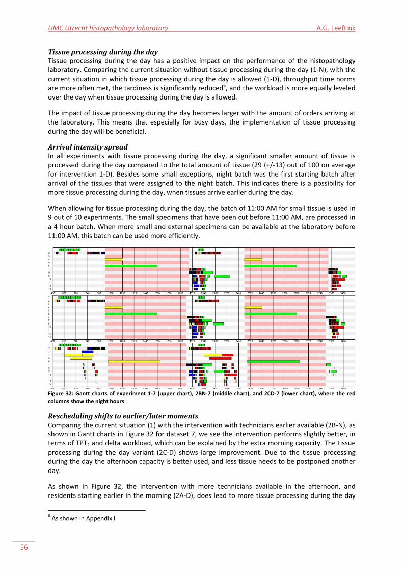
UMC Utrecht histopathology laboratory A.G. Leeftink
56
Tissue processing during the day Tissue processing during the day has a positive impact on the performance of the histopathology laboratory. Comparing the current situation without tissue processing during the day (1-N), with the current situation in which tissue processing during the day is allowed (1-D), throughput time norms are more often met, the tardiness is significantly reduced6, and the workload is more equally leveled over the day when tissue processing during the day is allowed.
The impact of tissue processing during the day becomes larger with the amount of orders arriving at the laboratory. This means that especially for busy days, the implementation of tissue processing during the day will be beneficial.
Arrival intensity spread In all experiments with tissue processing during the day, a significant smaller amount of tissue is processed during the day compared to the total amount of tissue (29 (+/-13) out of 100 on average for intervention 1-D). Besides some small exceptions, night batch was the first starting batch after arrival of the tissues that were assigned to the night batch. This indicates there is a possibility for more tissue processing during the day, when tissues arrive earlier during the day.
When allowing for tissue processing during the day, the batch of 11:00 AM for small tissue is used in 9 out of 10 experiments. The small specimens that have been cut before 11:00 AM, are processed in a 4 hour batch. When more small and external specimens can be available at the laboratory before 11:00 AM, this batch can be used more efficiently.
Figure 32: Gantt charts of experiment 1-7 (upper chart), 2BN-7 (middle chart), and 2CD-7 (lower chart), where the red columns show the night hours
Rescheduling shifts to earlier/later moments Comparing the current situation (1) with the intervention with technicians earlier available (2B-N), as shown in Gantt charts in Figure 32 for dataset 7, we see the intervention performs slightly better, in terms of TPT2 and delta workload, which can be explained by the extra morning capacity. The tissue processing during the day variant (2C-D) shows large improvement. Due to the tissue processing during the day the afternoon capacity is better used, and less tissue needs to be postponed another day.
As shown in Figure 32, the intervention with more technicians available in the afternoon, and residents starting earlier in the morning (2A-D), does lead to more tissue processing during the day
6 As shown in Appendix I
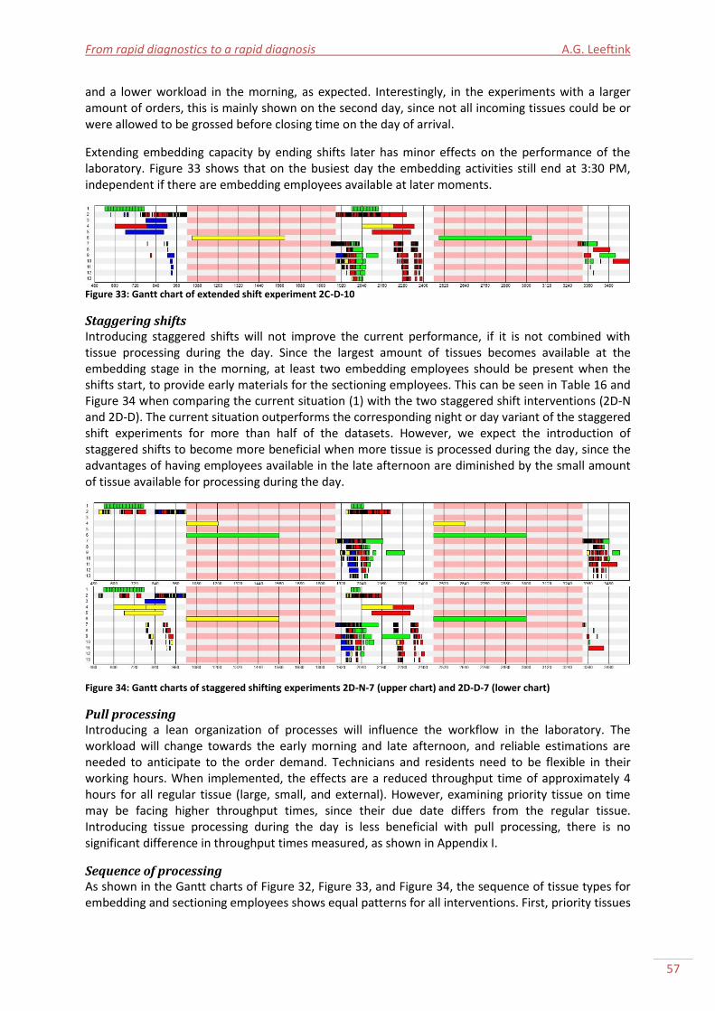
From rapid diagnostics to a rapid diagnosis A.G. Leeftink
57
and a lower workload in the morning, as expected. Interestingly, in the experiments with a larger amount of orders, this is mainly shown on the second day, since not all incoming tissues could be or were allowed to be grossed before closing time on the day of arrival.
Extending embedding capacity by ending shifts later has minor effects on the performance of the laboratory. Figure 33 shows that on the busiest day the embedding activities still end at 3:30 PM, independent if there are embedding employees available at later moments.
Figure 33: Gantt chart of extended shift experiment 2C-D-10
Staggering shifts Introducing staggered shifts will not improve the current performance, if it is not combined with tissue processing during the day. Since the largest amount of tissues becomes available at the embedding stage in the morning, at least two embedding employees should be present when the shifts start, to provide early materials for the sectioning employees. This can be seen in Table 16 and Figure 34 when comparing the current situation (1) with the two staggered shift interventions (2D-N and 2D-D). The current situation outperforms the corresponding night or day variant of the staggered shift experiments for more than half of the datasets. However, we expect the introduction of staggered shifts to become more beneficial when more tissue is processed during the day, since the advantages of having employees available in the late afternoon are diminished by the small amount of tissue available for processing during the day.
Figure 34: Gantt charts of staggered shifting experiments 2D-N-7 (upper chart) and 2D-D-7 (lower chart)
Pull processing Introducing a lean organization of processes will influence the workflow in the laboratory. The workload will change towards the early morning and late afternoon, and reliable estimations are needed to anticipate to the order demand. Technicians and residents need to be flexible in their working hours. When implemented, the effects are a reduced throughput time of approximately 4 hours for all regular tissue (large, small, and external). However, examining priority tissue on time may be facing higher throughput times, since their due date differs from the regular tissue. Introducing tissue processing during the day is less beneficial with pull processing, there is no significant difference in throughput times measured, as shown in Appendix I.
Sequence of processing As shown in the Gantt charts of Figure 32, Figure 33, and Figure 34, the sequence of tissue types for embedding and sectioning employees shows equal patterns for all interventions. First, priority tissues
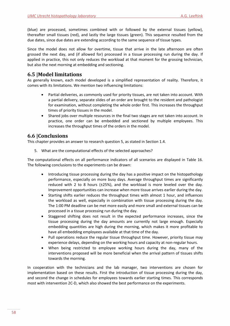
UMC Utrecht histopathology laboratory A.G. Leeftink
58
(blue) are processed, sometimes combined with or followed by the external tissues (yellow), thereafter small tissues (red), and lastly the large tissues (green). This sequence resulted from the due dates, since due dates are extending according to the same sequence of tissue types.
Since the model does not allow for overtime, tissue that arrive in the late afternoon are often grossed the next day, and (if allowed for) processed in a tissue processing run during the day. If applied in practice, this not only reduces the workload at that moment for the grossing technician, but also the next morning at embedding and sectioning.
6.5 |Model limitations As generally known, each model developed is a simplified representation of reality. Therefore, it comes with its limitations. We mention two influencing limitations:
Partial deliveries, as commonly used for priority tissues, are not taken into account. With a partial delivery, separate slides of an order are brought to the resident and pathologist for examination, without completing the whole order first. This increases the throughput times of priority tissues in the model.
Shared jobs over multiple resources in the final two stages are not taken into account. In practice, one order can be embedded and sectioned by multiple employees. This increases the throughput times of the orders in the model.
6.6 |Conclusions This chapter provides an answer to research question 5, as stated in Section 1.4.
5. What are the computational effects of the selected approaches?
The computational effects on all performance indicators of all scenarios are displayed in Table 16. The following conclusions to the experiments can be drawn:
Introducing tissue processing during the day has a positive impact on the histopathology performance, especially on more busy days. Average throughput times are significantly reduced with 2 to 8 hours (±25%), and the workload is more leveled over the day. Improvement opportunities can increase when more tissue arrives earlier during the day.
Starting shifts earlier reduces the throughput times with almost 1 hour, and influences the workload as well, especially in combination with tissue processing during the day. The 1:00 PM deadline can be met more easily and more small and external tissues can be processed in a tissue processing run during the day.
Staggered shifting does not result in the expected performance increases, since the tissue processing during the day amounts are currently not large enough. Especially embedding quantities are high during the morning, which makes it more profitable to have all embedding employees available at that time of the day.
Pull operations reduce the regular tissue throughput time. However, priority tissue may experience delays, depending on the working hours and capacity at non-regular hours.
When being restricted to employee working hours during the day, many of the interventions proposed will be more beneficial when the arrival pattern of tissues shifts towards the morning.
In cooperation with the technicians and the lab manager, two interventions are chosen for implementation based on these results. First the introduction of tissue processing during the day, and second the change in schedules for employees towards earlier starting times. This corresponds most with intervention 2C-D, which also showed the best performance on the experiments.
From rapid diagnostics to a rapid diagnosis A.G. Leeftink
59
Chapter 7 |Implementation This chapter describes the needed steps for implementation of the changes proposed in the previous chapters. This chapter uses these findings to propose implementation of tissue processing during the day, and earlier working times for technicians and residents, as combined in intervention 2C-D of Chapter 6. This requires several steps to be taken before the aimed results are seen. The project is regarded as successful, when the agreements agreed upon are followed, when the perceived workload of the technicians equals the average workload of the department, and when the targets on throughput times of the histopathology laboratory are met. This chapter will give an answer to the 6th research question, to achieve the goal of this study: realizing a rapid diagnosis for all patients, instead of rapid diagnostics for a selection of patients.
Section 7.1 gives a short introduction to the theory on improvement implementation. In Section 7.2 stakeholders are identified. Section 7.3 describes the changes needed in the current operations, and activities are identified to apply these changes. In Section 7.4 risks are identified. Section 7.5 comments on the evaluation and monitoring of the implementation, and we will end with conclusions in Section 7.6.
7.1 |Improvement implementation literature Implementation planning is important to ensure the outcome of improvement initiatives (Commonwealth of Australia, 2014a). Slack et al. (2007) consider two improvement strategies: The first is breakthrough improvement, which are large changes in the current practices, such as the redesign of the laboratory. The second is continuous improvement, in which more and smaller incremental improvements are strived for. Rescheduling the assignment of tissues to a certain machine and timing is an incremental improvement. First, biopsies can be processed in a tissue processing run during the day, hereafter other tissues follow. When continuously improving, not the rate of improvement is important, but the momentum of improvement (Slack et al., 2007, pp. 595). The improvements can be very small, but should take place every period.
An improvement cycle model, such as the PDCA cycle, can be used to structure the operational improvement. PDCA stands for Plan-Do-Check-Act. In an improvement environment, you first have to design a plan of action, thereafter you will implement the plan, you check and evaluate whether the plan results in the expected change in performance, and finally you act the improvement in your daily operations (Slack et al., 2007). The Do-stage includes the real implementation, where the implementation plan is already written in the Plan-stage.
Implementation should lead to a structural and sustainable change (Grol et al., 2013). To structure the process of implementation, a step-by-step planning is followed usually. Herein, special attention needs to be given to the innovation itself (Grol et al., 2013). To structure the development of the implementation plan we consider six areas (adapted from Commonwealth of Australia (2014a)):
1. Engaging stakeholders; 2. Planning; 3. Managing risk; 4. Monitoring, review, and evaluation; 5. Resource management; 6. Management strategy.
A successful implementation of improvement initiatives depends on several factors (Slack et al., 2007, and Grol et al., 2013):

UMC Utrecht histopathology laboratory A.G. Leeftink
60
First of all, the improvements should align with the (long term) strategy, to be successful in the long term, and to get the amount of resources needed, and management should show commitment to the improvements.
Second, the innovation should be integrated as much as possible in the current infrastructure. For example using the available information systems, because staff knows how to use these systems, or using the regular team meetings, because staff is already familiar with these meetings.
Third, specific people should be involved in the implementation phase, from several levels within the organization, which feel responsible for a successful implementation of the improvements and monitor the progress.
Fourth, the operating staff, such as the technicians, should work together in teams to learn from each other and be able to continuously improve. Furthermore, they should be included in the development, adaption, and planning of the innovation.
Fifth, the level of measuring and evaluating performance should be adapted to the level at which it is presented. Furthermore, the assessment during the implementation process should be continuously performed.
Sixth, the strategy for successful adaption of changes in medium sized groups, such as the technicians, is to ensure opinion figures and key persons are in favor of the innovation.
Seventh and last, the efforts of the operating staff in the implementation should be recognized and commented upon.
7.2 |Stakeholder engagement We already saw that involving the right people in the implementation of an initiative will increase the chances of success. Stakeholder engagement therefore is one of the key things to consider.
According to the definition of Freeman (1984), stakeholders are “any group or individual who can affect or is affected by the achievement of the firm’s objectives.” Key stakeholders and their influence in this improvement trajectory are:
Technicians, whose working conditions will change. They have to commit to the changes. Therefore, they have to be involved in the implementation phase from the beginning;
Residents, whose working conditions will slightly change. The work in the histopathology laboratory is not necessarily their main job, and the improvement trajectory is not necessarily of interest to them. Therefore, they may be less committed to optimizing the workflow in the histopathology laboratory. They have to commit to the changes proposed. Their involvement can be reduced to regularly sharing information on the progress that is made so far, but they have to be involved from the start of the implementation phase;
Pathologists, whose working conditions will change. They make the final decisions on their own work together with the head of the department of Pathology. The involvement can be reduced to regularly sharing information on the progress that is made so far;
Lab manager, who is responsible for the performance of the histopathology laboratory and is engaged in monitoring and evaluating the histopathology laboratory. She has to be extensively involved in the implementation phase from the beginning, especially in monitoring performance;
Head of the department of Pathology, who is the final decision maker. He has to be kept informed during the whole project.
Other important stakeholders are the customers. However, since they are not likely to be negatively influenced through the operational changes, we do not involve them in our implementation plan. We consider two customer types:
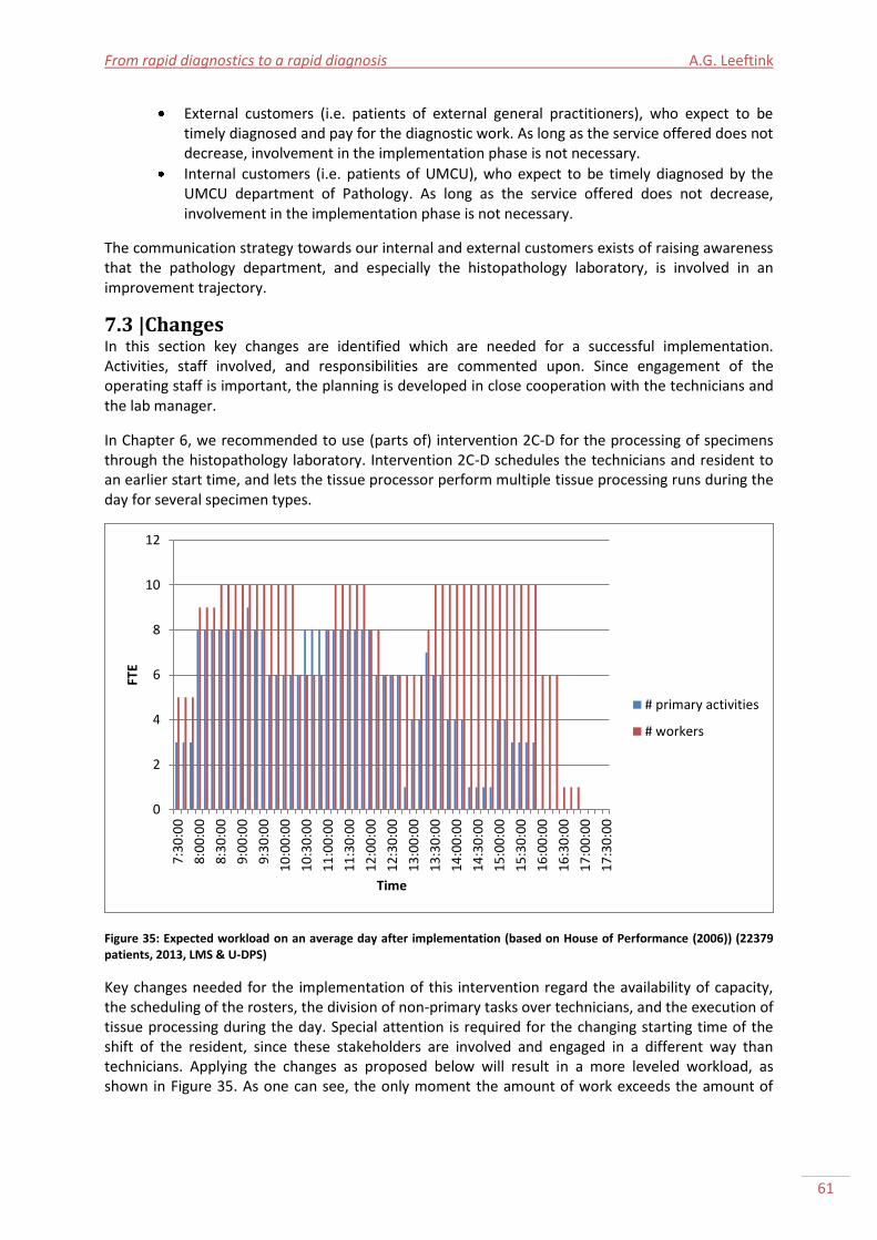
From rapid diagnostics to a rapid diagnosis A.G. Leeftink
61
External customers (i.e. patients of external general practitioners), who expect to be timely diagnosed and pay for the diagnostic work. As long as the service offered does not decrease, involvement in the implementation phase is not necessary.
Internal customers (i.e. patients of UMCU), who expect to be timely diagnosed by the UMCU department of Pathology. As long as the service offered does not decrease, involvement in the implementation phase is not necessary.
The communication strategy towards our internal and external customers exists of raising awareness that the pathology department, and especially the histopathology laboratory, is involved in an improvement trajectory.
7.3 |Changes In this section key changes are identified which are needed for a successful implementation. Activities, staff involved, and responsibilities are commented upon. Since engagement of the operating staff is important, the planning is developed in close cooperation with the technicians and the lab manager.
In Chapter 6, we recommended to use (parts of) intervention 2C-D for the processing of specimens through the histopathology laboratory. Intervention 2C-D schedules the technicians and resident to an earlier start time, and lets the tissue processor perform multiple tissue processing runs during the day for several specimen types.
Figure 35: Expected workload on an average day after implementation (based on House of Performance (2006)) (22379 patients, 2013, LMS & U-DPS)
Key changes needed for the implementation of this intervention regard the availability of capacity, the scheduling of the rosters, the division of non-primary tasks over technicians, and the execution of tissue processing during the day. Special attention is required for the changing starting time of the shift of the resident, since these stakeholders are involved and engaged in a different way than technicians. Applying the changes as proposed below will result in a more leveled workload, as shown in Figure 35. As one can see, the only moment the amount of work exceeds the amount of
0
2
4
6
8
10
12
7:3
0:0
0
8:0
0:0
0
8:3
0:0
0
9:0
0:0
0
9:3
0:0
0
10
:00
:00
10
:30
:00
11
:00
:00
11
:30
:00
12
:00
:00
12
:30
:00
13
:00
:00
13
:30
:00
14
:00
:00
14
:30
:00
15
:00
:00
15
:30
:00
16
:00
:00
16
:30
:00
17
:00
:00
17
:30
:00
FTE
Time
# primary activities
# workers
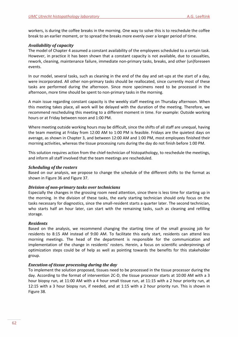
UMC Utrecht histopathology laboratory A.G. Leeftink
62
workers, is during the coffee breaks in the morning. One way to solve this is to reschedule the coffee break to an earlier moment, or to spread the breaks more evenly over a longer period of time.
Availability of capacity The model of Chapter 4 assumed a constant availability of the employees scheduled to a certain task. However, in practice it has been shown that a constant capacity is not available, due to casualties, rework, cleaning, maintenance failure, immediate non-primary tasks, breaks, and other (un)foreseen events.
In our model, several tasks, such as cleaning in the end of the day and set-ups at the start of a day, were incorporated. All other non-primary tasks should be reallocated, since currently most of these tasks are performed during the afternoon. Since more specimens need to be processed in the afternoon, more time should be spent to non-primary tasks in the morning.
A main issue regarding constant capacity is the weekly staff meeting on Thursday afternoon. When this meeting takes place, all work will be delayed with the duration of the meeting. Therefore, we recommend rescheduling this meeting to a different moment in time. For example: Outside working hours or at Friday between noon and 1:00 PM.
Where meeting outside working hours may be difficult, since the shifts of all staff are unequal, having the team meeting at Friday from 12:00 AM to 1:00 PM is feasible. Fridays are the quietest days on average, as shown in Chapter 3, and between 12:00 AM and 1:00 PM, most employees finished their morning activities, whereas the tissue processing runs during the day do not finish before 1:00 PM.
This solution requires action from the chief-technician of histopathology, to reschedule the meetings, and inform all staff involved that the team meetings are rescheduled.
Scheduling of the rosters Based on our analysis, we propose to change the schedule of the different shifts to the format as shown in Figure 36 and Figure 37.
Division of non-primary tasks over technicians Especially the changes in the grossing room need attention, since there is less time for starting up in the morning. In the division of these tasks, the early starting technician should only focus on the tasks necessary for diagnostics, since the small-resident starts a quarter later. The second technician, who starts half an hour later, can start with the remaining tasks, such as cleaning and refilling storage.
Residents Based on the analysis, we recommend changing the starting time of the small grossing job for residents to 8:15 AM instead of 9:00 AM. To facilitate this early start, residents can attend less morning meetings. The head of the department is responsible for the communication and implementation of the change in residents’ rosters. Herein, a focus on scientific underpinnings of optimization steps could be of help as well as pointing towards the benefits for this stakeholder group.
Execution of tissue processing during the day To implement the solution proposed, tissues need to be processed in the tissue processor during the day. According to the format of intervention 2C-D, the tissue processor starts at 10:00 AM with a 3 hour biopsy run, at 11:00 AM with a 4 hour small tissue run, at 11:15 with a 2 hour priority run, at 12:15 with a 3 hour biopsy run, if needed, and at 1:15 with a 2 hour priority run. This is shown in Figure 38.
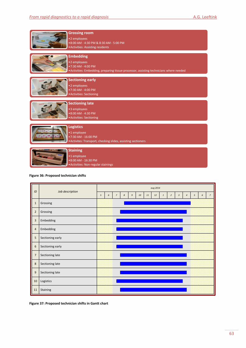
From rapid diagnostics to a rapid diagnosis A.G. Leeftink
63
Figure 36: Proposed technician shifts
ID Job descriptionaug 2014
5 6 7 8 9 10 11 12 1 2 3
1 Grossing
2 Grossing
3 Embedding
4 Embedding
5 Sectioning early
6 Sectioning early
7 Sectioning late
8 Sectioning late
9 Sectioning late
10 Logistics
11 Staining
4 5 6 7
Figure 37: Proposed technician shifts in Gantt chart
Grossing room
•2 employees
•8:00 AM - 4:30 PM & 8:30 AM - 5:00 PM
•Activities: Assisting residents
Embedding
•2 employees
•7:30 AM - 4:00 PM
•Activities: Embedding, preparing tissue processor, assisting technicians where needed
Sectioning early
•2 employees
•7:30 AM - 4:00 PM
•Activities: Sectioning
Sectioning late
•3 employees
•8:00 AM - 4:30 PM
•Activities: Sectioning
Logistics
•1 employee
•7:30 AM - 16:00 PM
•Activites: Transport, checking slides, assisting sectioners
Staining
•1 employee
•8:00 AM - 16:30 PM
•Activities: Non-regular stainings
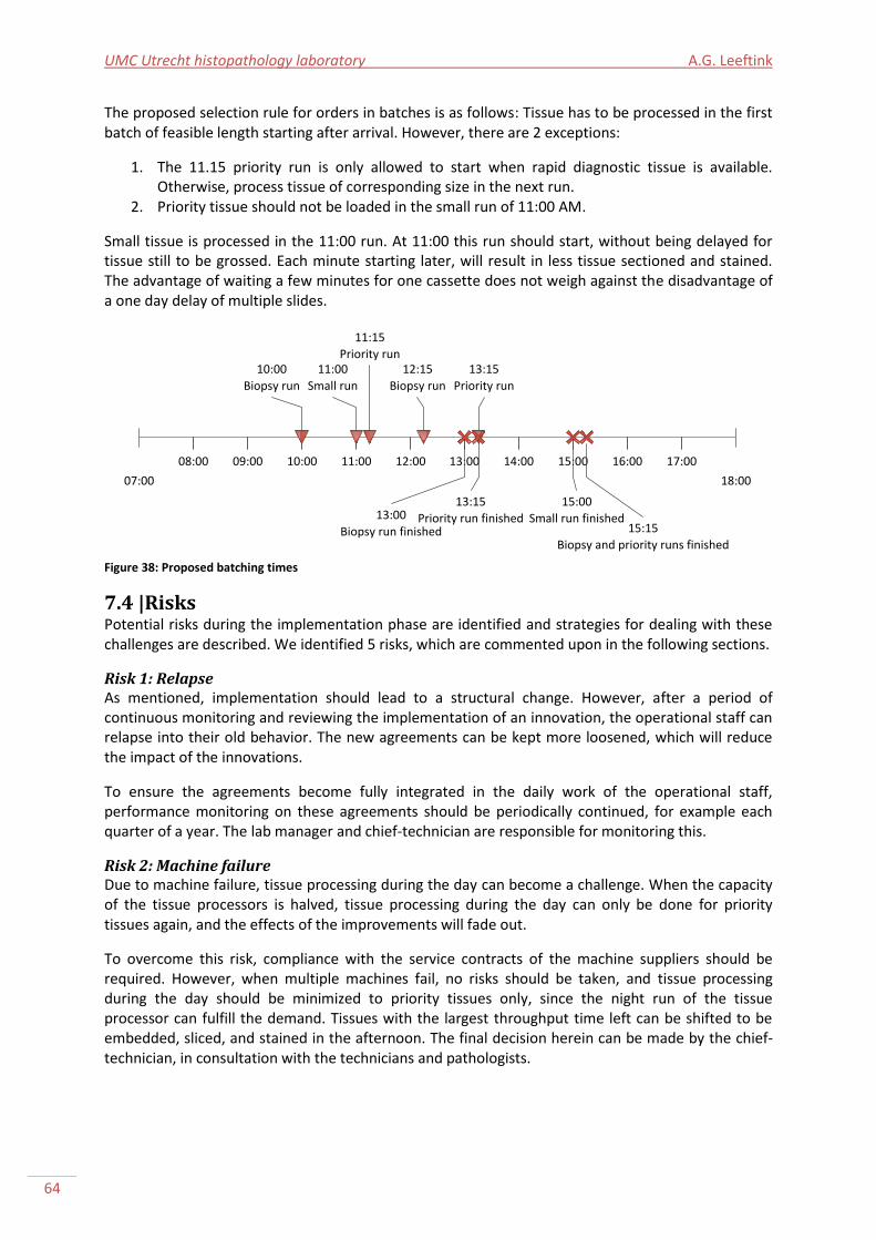
UMC Utrecht histopathology laboratory A.G. Leeftink
64
The proposed selection rule for orders in batches is as follows: Tissue has to be processed in the first batch of feasible length starting after arrival. However, there are 2 exceptions:
1. The 11.15 priority run is only allowed to start when rapid diagnostic tissue is available. Otherwise, process tissue of corresponding size in the next run.
2. Priority tissue should not be loaded in the small run of 11:00 AM.
Small tissue is processed in the 11:00 run. At 11:00 this run should start, without being delayed for tissue still to be grossed. Each minute starting later, will result in less tissue sectioned and stained. The advantage of waiting a few minutes for one cassette does not weigh against the disadvantage of a one day delay of multiple slides.
07:00 18:00
08:00 09:00 10:00 11:00 12:00 13:00 14:00 15:00 16:00 17:00
11:15
Priority run12:15
Biopsy run
13:15
Priority run
10:00
Biopsy run
11:00
Small run
13:00
Biopsy run finished
15:00
Small run finished
13:15
Priority run finished15:15
Biopsy and priority runs finished
Figure 38: Proposed batching times
7.4 |Risks Potential risks during the implementation phase are identified and strategies for dealing with these challenges are described. We identified 5 risks, which are commented upon in the following sections.
Risk 1: Relapse As mentioned, implementation should lead to a structural change. However, after a period of continuous monitoring and reviewing the implementation of an innovation, the operational staff can relapse into their old behavior. The new agreements can be kept more loosened, which will reduce the impact of the innovations.
To ensure the agreements become fully integrated in the daily work of the operational staff, performance monitoring on these agreements should be periodically continued, for example each quarter of a year. The lab manager and chief-technician are responsible for monitoring this.
Risk 2: Machine failure Due to machine failure, tissue processing during the day can become a challenge. When the capacity of the tissue processors is halved, tissue processing during the day can only be done for priority tissues again, and the effects of the improvements will fade out.
To overcome this risk, compliance with the service contracts of the machine suppliers should be required. However, when multiple machines fail, no risks should be taken, and tissue processing during the day should be minimized to priority tissues only, since the night run of the tissue processor can fulfill the demand. Tissues with the largest throughput time left can be shifted to be embedded, sliced, and stained in the afternoon. The final decision herein can be made by the chief-technician, in consultation with the technicians and pathologists.
From rapid diagnostics to a rapid diagnosis A.G. Leeftink
65
Risk 3: Pointing to the neighbor The current improvement step is aimed at the histopathology laboratory. However, for a full optimization, the examination step at the residents’ and pathologists’’ desks should be reviewed and optimized as well. As shown in literature, the efforts of the operating staff, which are the technicians, in the implementation should be recognized and commented upon. However, when the optimization of the examination step is hold off, technicians can feel unrecognized and the target of continuous improvement. This can result in pointing to the (large) possibilities of improvement at their neighbor, and less commitment to continuously improving in their own laboratory.
To overcome this risk, the lab manager and the head of the department should show commitment to the innovations. Possibilities for optimizing the examination phase should not only be discussed with the residents and pathologists, but (a delegation of the) technicians should attend as well.
Risk 4: Negative effect for customers Even though the model showed the throughput times will be minimized after a full implementation, and a decrease in performance is unexpected, an increase in throughput times could occur due to the changed working conditions. When this happens, patients have to wait longer before being diagnosed, which is extremely undesirable.
To overcome this risk, continuous monitoring needs to be done during the implementation trajectory on throughput times. Every week, during the weekly meeting with technicians, this should be discussed. The chief-technician is responsible for this performance monitoring. Challenges are therefore identified and dealt with in an early stage.
Risk 5: Sub-optimization Since the histopathology laboratory optimization is art of a larger improvement trajectory of the department of Pathology, it is important to realize the risk for sub-optimization. Reducing the throughput times in the histopathology laboratory with, for example, 6 hours, does not reduce the overall throughput times when the residents and pathologists keep their current examination moments. In that case, slides will remain for 6 extra hours on their desks.
The same applies to the frond-end processes. Chapter 6 showed large benefits could be won when the arrivals at the laboratory are better regulated (less batching, earlier deliveries). Recently, a project was started to research the costs and benefits of tubing, which could reduce the batching incidence from internal customers at the patient administration.
Concluding, it is important to continue the improvement trajectory, by looking at the examination process and the scheduling of pathologists tasks over the day/week, and by looking at the logistics around the flow of tissues from clinics to the patient administration.
7.5 |Monitoring, review, and evaluation To control the implementation process, monitoring, review, and evaluation activities not only improve the success and reliability of the implementation, but also help in decision making (Commonwealth of Australia, 2014a).
Evaluation comments on the effectiveness (do we do the right thing, do we get the expected results?), efficiency (do we do it the right way, do we make good use of our resources?), and find opportunities for improvement. These questions should be answered in every monitoring, review, and evaluation meeting (Commonwealth of Australia, 2014b). Important elements of a successful monitoring, review, and evaluation, are reviewing regularly, reporting frequently, and involving relevant stakeholders (Commonwealth of Australia, 2014b).
As already said, the lab manager and the chief-technician are together responsible for monitoring of the implementation. Continuous monitoring needs to be done during the implementation trajectory
UMC Utrecht histopathology laboratory A.G. Leeftink
66
on throughput times, to reduce the risk on negative effects for customers and to ensure continuity in the project. It is the responsibility of the chief-technician to discuss the performance and questions mentioned during the weekly meeting with technicians, but also to ensure that the findings of the evaluation sessions are applied in continuous improvement.
In the ´werkbelevingsonderzoek´, which is held every two years, the workload is reviewed. This can be compared to the previous performance, and should be shown to the technicians when available. Next to the workload, the throughput times should be visible for the technicians as well. These should be shown together with the past performance and the targets.
The data needed for performance evaluation, can be gathered making use of (existing) functions in LMS. The chief-technician and lab manager should together decide which performance indicators to use, and, if necessary, ask for the developers of LMS to include that in the next release of LMS. A performance measure suggestion which make the amount of tissues processed during the day visible for the technicians is the percentage of tissues processed in a tissue processing run during the day compared to the night run.
After about 3 months a first evaluation meeting should be held with the key-stakeholders involved, as well as 1 year after the implementation. The lab manager should be responsible for the organization of this meeting.
7.6 |Conclusions This section provides a conclusion to this chapter, and an answer to the sixth research question, as described in Section 1.4.
6. What steps are needed to implement the selected approaches?
To successfully implement the proposed interventions resulting from Chapter 6, several tasks have to be performed within a time frame of a year. These tasks include the involvement of stakeholders, changing the availability of capacity, changing the scheduling of the rosters, changing the division of non-primary tasks over technicians, and the execution of tissue processing during the day. Special attention is required for the changing starting time of the shift of the resident, since these stakeholders are involved and engaged in a different way than technicians.
It is important to continue the improvement trajectory, by looking at the examination process and the scheduling of pathologists tasks over the day/week, and by looking at the logistics around the flow of tissues from clinics to the patient administration. Furthermore, attention is needed for risk monitoring, monitoring the progress of the project, and a final evaluation.
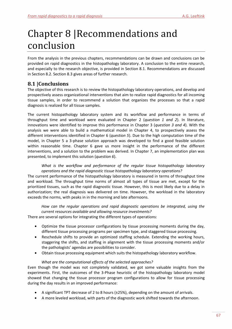
From rapid diagnostics to a rapid diagnosis A.G. Leeftink
67
Chapter 8 |Recommendations and conclusion From the analysis in the previous chapters, recommendations can be drawn and conclusions can be provided on rapid diagnostics in the histopathology laboratory. A conclusion to the entire research, and especially to the research objective, is provided in Section 8.1. Recommendations are discussed in Section 8.2. Section 8.3 gives areas of further research.
8.1 |Conclusions The objective of this research is to review the histopathology laboratory operations, and develop and prospectively assess organizational interventions that aim to realize rapid diagnostics for all incoming tissue samples, in order to recommend a solution that organizes the processes so that a rapid diagnosis is realized for all tissue samples.
The current histopathology laboratory system and its workflow and performance in terms of throughput time and workload were evaluated in Chapter 2 (question 1 and 2). In literature, innovations were identified to improve this performance in Chapter 3 (question 3 and 4). With the analysis we were able to build a mathematical model in Chapter 4, to prospectively assess the different interventions identified in Chapter 6 (question 5). Due to the high computation time of the model, in Chapter 5 a 3-phase solution approach was developed to find a good feasible solution within reasonable time. Chapter 6 gave us more insight in the performance of the different interventions, and a solution to the problem was derived. In Chapter 7, an implementation plan was presented, to implement this solution (question 6).
What is the workflow and performance of the regular tissue histopathology laboratory operations and the rapid diagnostic tissue histopathology laboratory operations?
The current performance of the histopathology laboratory is measured in terms of throughput time and workload. The throughput time norms of almost all types of tissue are met, except for the prioritized tissues, such as the rapid diagnostic tissue. However, this is most likely due to a delay in authorization; the real diagnosis was delivered on time. However, the workload in the laboratory exceeds the norms, with peaks in in the morning and late afternoons.
How can the regular operations and rapid diagnostic operations be integrated, using the current resources available and allowing resource investments?
There are several options for integrating the different types of operations:
Optimize the tissue processor configurations by tissue processing moments during the day, different tissue processing programs per specimen type, and staggered tissue processing.
Reschedule shifts to provide an optimized staffing schedule. Extending the working hours, staggering the shifts, and staffing in alignment with the tissue processing moments and/or the pathologists’ agendas are possibilities to consider.
Obtain tissue processing equipment which suits the histopathology laboratory workflow.
What are the computational effects of the selected approaches? Even though the model was not completely validated, we got some valuable insights from the experiments. First, the outcomes of the 3-Phase heuristic of the histopathology laboratory model showed that changing the tissue processor program configurations to allow for tissue processing during the day results in an improved performance:
A significant TPT decrease of 2 to 8 hours (±25%), depending on the amount of arrivals.
A more leveled workload, with parts of the diagnostic work shifted towards the afternoon.
UMC Utrecht histopathology laboratory A.G. Leeftink
68
Second, the outcomes of the 3-Phase heuristic of the histopathology laboratory model suggested adaptions in the staffing schedules, to improve the performance:
Earlier starting times of technicians and residents. Due to the earlier starting times of the grossing technician and residents, more tissue can be processed during the day. Due to the earlier starting times for embedding and sectioning technicians, the 1:00 PM deadline can be met more often, which lowers the workload. Furthermore, it decreased the throughput time.
No staggered shifting. Due to the small tissue processing amounts during the day, staggered shifts in the different stages does not improve performance.
Tissue that arrives in the late afternoon, and cannot be grossed before the end of the shift that day, can be processed in a tissue processing run during the next day. This reduces the workload at that moment, but also the next morning at embedding and sectioning. Furthermore, it reduces the amount of overtime needed.
What steps are needed to implement the selected approaches? In cooperation with the technicians and the lab manager, two interventions are chosen for implementation based on these results. First the introduction of tissue processing during the day, and second the change in schedules for employees towards earlier starting times.
To successfully implement these interventions, several tasks have to be performed within a time frame of a year. These tasks include the involvement of stakeholders, changing the availability of capacity and non-primary tasks, changing the scheduling of the rosters of technicians and residents, and the execution of tissue processing during the day. Furthermore, attention is needed for risk monitoring, monitoring the progress of the project, and a final evaluation.
8.2 |Recommendations From the analysis, recommendations are provided for the histopathology laboratory at UMC Utrecht, to improve the process flow, to provide a rapid diagnosis for all incoming tissues. These include:
Introduce tissue processing during the day at the histopathology laboratory, for different types of tissue, including external and small tissues.
To be able to process small tissue during the day, the small grossing resident and technician shifts should start approximately 1 hour earlier.
To reduce the risk of sub-optimization it is important to continue the improvement trajectory by researching the examination process and the arrival process.
8.3 |Further research During the analysis of the performance of the histopathology laboratory at UMC Utrecht, various areas of study were identified that were out of scope of this project due to data or time limitation. This section discusses these areas, and present recommendations for further research.
Histopathology laboratory operations in general The histopathology laboratory is a complex system. Therefore, there are many opportunities for further research in this area:
Development of KPIs is needed to involve technicians in the evaluation of processes and awareness for improvement. This includes a more formalized way to measure performance, the development of (visible) KPI tools and its use in the histopathology laboratory.
Enhance the process by digital ordering for more insight in the arrivals.
Remove the use of registration forms in the histopathology laboratory. This reduces the amount of paper handling errors and increases the amount of data for KPI-measurements.
Extend process by digital examination, which includes scanning slides.
From rapid diagnostics to a rapid diagnosis A.G. Leeftink
69
Large gains can be derived in the arrival process. Bulk arrivals in the afternoon should be eliminated. These batch arrivals could be due to customer batching. Smoothening these arrivals, especially shifting them to the morning, will enlarge tissue processing during the day, and therefore reduce the workload and throughput times.
Within the pathology lean trajectory, there are plans for a complete reorganization of the histopathology laboratory. In this reorganization, attention should be paid to the sequence of tasks and desks, and to obtaining resources that match the process flow.
Tissue processor configurations There are several opportunities for further research regarding the tissue processor configurations:
Possibilities to tailor the tissue processor programs to fixation level exist and should be explored, since this can severely reduce the service times of the tissue processor.
It should be investigated if part of the large tissues can be run in a tissue processing run during the day as well, since they have been fixated long enough. Cutting tissues earlier, and process them in a tissue processing run during the day, would decrease the delta workload, and decrease the TPT. When possible, there might be an opportunity to let technicians gross (parts of) these specimens. This makes grossing less restricted to the residents agendas, and offers possibilities for tissue processing during the day.
There is an opportunity for further research on machine failure. The tissue processors have shown to fail frequently during the research period. Research into the failure of these machines may offer more insight in the failure pattern and offer a more efficient solution than the current solution (more capacity and reserving capacity).
Research is needed towards the 1:00 PM-deadline. Experienced residents could receive the slides later (i.e. 3:00 PM), and still be ready with examination on time.
Further development of the model The following options are given for further research regarding the development of the model:
Currently, the MILP-model requires a large computation time when using the datasets of the UMCU laboratory. Research is needed reduce the calculation time and memory usage. For example by further looking into vaalid inequalities or symmetry breaking constraints.
The 3-phase heuristic can be improved by using smarter scheduling rules, introducing priorities, or by adding an improvement heuristic after the construction heuristic.
Research is needed to determine the optimal batch starting times. Interesting similarities exist with the block scheduling of a Master Surgery Schedule, which can be a direction for further research. Another option is further research in arrival intensity based batch times.
Further research is needed on multiple criteria optimization: An (extra) objective to consider is to minimize the throughput time (= maximize earliness). However, this requires more computation time. Other options are to minimize the number of batches given the minimum tardiness (miNlp), to minimize the number of employees, to minimize the number of tardy orders (see constraints (13) and (17) in Mendez (2000)) or a combination of these objectives.
A sensitivity analysis on the parameters may result in more insight in the choice of parameter values. For example the priorities and due dates can be subject to a sensitivity analysis. The combination of both parameters can result in an increased prioritization effect, since both parameters are indicators of importance and prioritize the same way.
According to the model, 5 employees are continuously cutting paraffin sections in the morning. However, in practice, 5 sectioning employees are not always present, due to unexpected events, breaks, and other tasks. Further research could be performed to the effect of capacity fluctuations, for example to determine optimal break times.
When the processes in the histopathology laboratory are extended with digital ordering and digital scanning, the model can be adapted to include these stages as well.
UMC Utrecht histopathology laboratory A.G. Leeftink
70
References AIMMS. (2014). About us. Retrieved May 12, 2014, from http://business.aimms.com/about-us/
Brown, L. (2004). Improving histopathology turnaround time: a process management approach. In: Current Diagnostic Pathology. 10, 444-452.
Brown, J.R. (2009). Histologic Preparations: Common Problems and Their Solutions. Northfield, IL: College of American Pathologists.
Buesa, R.J. (2007). Microwave-assisted tissue processing: real impact on the histology workflow. In: Annals of Diagnostic Pathology. 11, 206-211.
Buesa, R.J. (2009). Adapting lean to histology laboratories [Technical Note]. In: Annals of Diagnostic Pathology. 13, 322-333.
Commonwealth of Austalia. (2014a). Implementation planning for the Australian Public Service. Guide to implementation planning. Retrieved from: https://www.dpmc.gov.au/implementation/planning.cfm.
Commonwealth of Austalia. (2014b). Implementation planning for the Australian Public Service. Monitoring, review and evaluation. Retrieved from: https://www.dpmc.gov.au/implementation/planning.cfm.
Freeman, R. E. (1984). Strategic management: A stakeholder approach. Boston: Pitman.
Grol, R., Wensing, M., Eccles, M., & Davis, D. (Eds.). (2013). Improving patient care: the implementation of change in health care. Chichester: John Wiley & Sons.
Gupta, S., and Karimi, I.A. (2003). An improved MILP formulation for scheduling multiproduct, multistage batch plants. In: Industrial & engineering chemistry research. 42(11), 2365-2380.
Kallrath, J. (2002). Planning and scheduling in the process industry. In: OR Spectrum. 24(3), 219-250.
Law, A.M. (2007). Simulation modeling and analysis. 4th edition. New York: McGraw-Hill.
Méndez, C.A., Cerdá, J., Grossmann, I.E., Harjunkoski, I., and Fahl, M. (2006). State-of-the-art review of optimization methods for short-term scheduling of batch processes. In: Computers & Chemical Eningeering. 30(6), 913-946.
Méndez, C.A., Henning, G.P., and Cerda, J. (2000). Optimal scheduling of batch plants satisfying multiple product orders with different due-dates. In: Computers & Chemical Engineering. 24(9), 2223-2245.
Muirhead, D., Aoun, P., Powell, M., Juncker, F., and Mollerup, J. (2009). Pathology Economic Model Tool. A novel approach to workflow and budget cost analysis in an anatomic pathology laboratory. In: Arch. Pathol. Lab. Med. 134, 1164-1169.
Munkholm, J., Talman, M.J., and Hasselager, T. (2008). Implementation of a new rapid tissue processing method – Advantages and challenges. In: Pathology – Research and Practice. 204: 899-904.
Patel, S., Smith, J.B., Kurbatova, E., and Guarner, J. (2011). Factors that impact turnaround time of surgical pathology specimens in an academic institution. In: Human Pathology. 43: 1501-1505.

From rapid diagnostics to a rapid diagnosis A.G. Leeftink
71
Pathologie. (2013). Kwaliteitshandboek pathologie. Retrieved from: http://magnus/kwaliteitsdocumenten/00025313.html
Prasad, P., and Maravelias, C.T. (2008). Batch selection, assignment and sequencing in multi-stage multi-product processes. In: Computers & Chemical Engineering. 32(6), 1106-1119.
Raad van Bestuur. (2012). Directieverslag 2012. Retrieved from: http://www.umcutrecht.nl/Directieverslag2012/
Ribé, A., Ribalta, T., Lledó, R. Torras, G., Asenjo, M.A., and Cardesa, A. (1998). Evaluation of turnaround times as component of quality assurance in surgical pathology. In: International Journal for Quality in Health Care. 10(3): 241-245.
Royal College of Pathologists. (2012). Key performance indicators in pathology. Retrieved from: https://www.rcpath.org/Resources/RCPath/Migrated%20Resources/Documents/K/key_performance_indicators_in_pathology_3_2.pdf
Sambeek, J. van. (2005). Het opereren van het werk op de OK. Enschede: Universiteit Twente.
Serrano, L., Hegge, P., Sato, B., Richmond, B., and Stahnke, L. (2010). Using LEAN principles to improve quality, patient safety, and workflow in histology and anatomic pathology. In: Adv. Anat. Pathol. 17(3): 215-221.
Slack, N., Chambers, S., & Johnston, R. (2007). Operations management. [5th edition]. Harlow: Pearson Education.
UMC Utrecht. (2014a). Mission. Retrieved from: http://www.umcutrecht.nl/overumcutrecht/missie
UMC Utrecht. (2014b). Pathology. Retrieved from: http://www.pathologieutrecht.nl/
UMC Utrecht. (2013a). Einddocument Sneldiagnose Pathologie. [Powerpoint Presentation].
UMC Utrecht. (2013b). Pathologie jaarverslag 2012.
UMC Utrecht (2006). House of Performance.
Vanberkel, P.T, Boucherie, R.J., Hans, E.W., Hurink, J.L., Litvak, N. (2012). Efficiency evaluation for pooling resources in health care. In: OR Spectrum, 34(2), 371-390.
Vernon, S.E. (2005). Continuous throughput rapid tissue processing revolutionizes histopathology workflow. In: Labmedicine. 36(5): 300-302.
Zonderland, M.E., & Timmer, J. (2012). Optimal allocation of MRI scan capacity among competing hospital departments. In: European Journal of Operations Research, 219(3), 630-637.

UMC Utrecht histopathology laboratory A.G. Leeftink
72
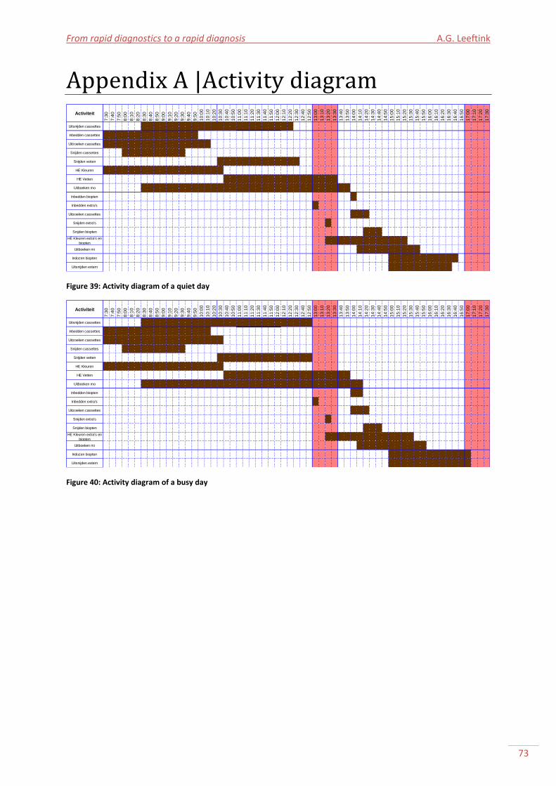
From rapid diagnostics to a rapid diagnosis A.G. Leeftink
73
Appendix A |Activity diagram
Figure 39: Activity diagram of a quiet day
Figure 40: Activity diagram of a busy day
Activiteit
7:3
0
7:4
0
7:5
0
8:0
0
8:1
0
8:2
0
8:3
0
8:4
0
8:5
0
9:0
0
9:1
0
9:2
0
9:3
0
9:4
0
9:5
0
10
:00
10
:10
10
:20
10
:30
10
:40
10
:50
11
:00
11
:10
11
:20
11
:30
11
:40
11
:50
12
:00
12
:10
12
:20
12
:30
12
:40
12
:50
13
:00
13
:10
13
:20
13
:30
13
:40
13
:50
14
:00
14
:10
14
:20
14
:30
14
:40
14
:50
15
:00
15
:10
15
:20
15
:30
15
:40
15
:50
16
:00
16
:10
16
:20
16
:30
16
:40
16
:50
17
:00
17
:10
17
:20
17
:30
Uitsnijden cassettes
Inbedden cassettes 9:58 9:58 9:58 9:58 9:58 9:58 9:58 9:58 9:58 9:58 9:58 9:58 9:58 9:58 9:58 9:58 9:58 9:58 9:58 9:58 9:58 9:58 9:58 9:58 9:58 9:58 9:58 9:58 9:58 9:58 9:58 9:58 9:58 9:58 9:58 9:58 9:58 9:58 9:58 9:58 9:58 9:58 9:58 9:58 9:58 9:58 9:58 9:58 9:58 9:58 9:58 9:58 9:58 9:58 9:58 9:58 9:58 9:58 9:58 9:58 9:58
Uitzoeken cassettes ### ### ### ### ### ### ### ### ### ### ### ### ### ### ### ### ### ### ### ### ### ### ### ### ### ### ### ### ### ### ### ### ### ### ### ### ### ### ### ### ### ### ### ### ### ### ### ### ### ### ### ### ### ### ### ### ### ### ### ### ###
Snijden cassettes 9:36 9:36 9:36 9:36 9:36 9:36 9:36 9:36 9:36 9:36 9:36 9:36 9:36 9:36 9:36 9:36 9:36 9:36 9:36 9:36 9:36 9:36 9:36 9:36 9:36 9:36 9:36 9:36 9:36 9:36 9:36 9:36 9:36 9:36 9:36 9:36 9:36 9:36 9:36 9:36 9:36 9:36 9:36 9:36 9:36 9:36 9:36 9:36 9:36 9:36 9:36 9:36 9:36 9:36 9:36 9:36 9:36 9:36 9:36 9:36 9:36
Snijden vetten ### ### ### ### ### ### ### ### ### ### ### ### ### ### ### ### ### ### ### ### ### ### ### ### ### ### ### ### ### ### ### ### ### ### ### ### ### ### ### ### ### ### ### ### ### ### ### ### ### ### ### ### ### ### ### ### ### ### ### ### ###
HE Kleuren ### ### ### ### ### ### ### ### ### ### ### ### ### ### ### ### ### ### ### ### ### ### ### ### ### ### ### ### ### ### ### ### ### ### ### ### ### ### ### ### ### ### ### ### ### ### ### ### ### ### ### ### ### ### ### ### ### ### ### ### ###
HE Vetten ### ### ### ### ### ### ### ### ### ### ### ### ### ### ### ### ### ### ### ### ### ### ### ### ### ### ### ### ### ### ### ### ### ### ### ### ### ### ### ### ### ### ### ### ### ### ### ### ### ### ### ### ### ### ### ### ### ### ### ### ###
Uitboeken mo ### ### ### ### ### ### ### ### ### ### ### ### ### ### ### ### ### ### ### ### ### ### ### ### ### ### ### ### ### ### ### ### ### ### ### ### ### ### ### ### ### ### ### ### ### ### ### ### ### ### ### ### ### ### ### ### ### ### ### ### ###
Inbedden biopten 0,6 0,6 0,6 0,6 0,6 0,6 0,6 0,6 0,6 0,6 0,6 0,6 0,6 0,6 0,6 0,6 0,6 0,6 0,6 0,6 0,6 0,6 0,6 0,6 0,6 0,6 0,6 0,6 0,6 0,6 0,6 0,6 0,6 0,6 0,6 0,6 0,6 0,6 0,6 0,6 0,6 0,6 0,6 0,6 0,6 0,6 0,6 0,6 0,6 0,6 0,6 0,6 0,6 0,6 0,6 0,6 0,6 0,6 0,6 0,6 0,6
Inbedden extra's 0,5 0,5 0,5 0,5 0,5 0,5 0,5 0,5 0,5 0,5 0,5 0,5 0,5 0,5 0,5 0,5 0,5 0,5 0,5 0,5 0,5 0,5 0,5 0,5 0,5 0,5 0,5 0,5 0,5 0,5 0,5 0,5 0,5 0,5 0,5 0,5 0,5 0,5 0,5 0,5 0,5 0,5 0,5 0,5 0,5 0,5 0,5 0,5 0,5 0,5 0,5 0,5 0,5 0,5 0,5 0,5 0,5 0,5 0,5 0,5 0,5
Uitzoeken cassettes 0,6 0,6 0,6 0,6 0,6 0,6 0,6 0,6 0,6 0,6 0,6 0,6 0,6 0,6 0,6 0,6 0,6 0,6 0,6 0,6 0,6 0,6 0,6 0,6 0,6 0,6 0,6 0,6 0,6 0,6 0,6 0,6 0,6 0,6 0,6 0,6 0,6 0,6 0,6 0,6 0,6 0,6 0,6 0,6 0,6 0,6 0,6 0,6 0,6 0,6 0,6 0,6 0,6 0,6 0,6 0,6 0,6 0,6 0,6 0,6 0,6
Snijden extra's 0,6 0,6 0,6 0,6 0,6 0,6 0,6 0,6 0,6 0,6 0,6 0,6 0,6 0,6 0,6 0,6 0,6 0,6 0,6 0,6 0,6 0,6 0,6 0,6 0,6 0,6 0,6 0,6 0,6 0,6 0,6 0,6 0,6 0,6 0,6 0,6 0,6 0,6 0,6 0,6 0,6 0,6 0,6 0,6 0,6 0,6 0,6 0,6 0,6 0,6 0,6 0,6 0,6 0,6 0,6 0,6 0,6 0,6 0,6 0,6 0,6
Snijden biopten 0,6 0,6 0,6 0,6 0,6 0,6 0,6 0,6 0,6 0,6 0,6 0,6 0,6 0,6 0,6 0,6 0,6 0,6 0,6 0,6 0,6 0,6 0,6 0,6 0,6 0,6 0,6 0,6 0,6 0,6 0,6 0,6 0,6 0,6 0,6 0,6 0,6 0,6 0,6 0,6 0,6 0,6 0,6 0,6 0,6 0,6 0,6 0,6 0,6 0,6 0,6 0,6 0,6 0,6 0,6 0,6 0,6 0,6 0,6 0,6 0,6
HE Kleuren extra's en
biopten0,6 0,6 0,6 0,6 0,6 0,6 0,6 0,6 0,6 0,6 0,6 0,6 0,6 0,6 0,6 0,6 0,6 0,6 0,6 0,6 0,6 0,6 0,6 0,6 0,6 0,6 0,6 0,6 0,6 0,6 0,6 0,6 0,6 0,6 0,6 0,6 0,6 0,6 0,6 0,6 0,6 ### 0,6 0,6 0,6 0,6 0,6 0,6 0,6 0,6 0,6 0,6 0,6 0,6 0,6 0,6 0,6 0,6 0,6 0,6 0,6
Uitboeken mi 0,7 0,7 0,7 0,7 0,7 0,7 0,7 0,7 0,7 0,7 0,7 0,7 0,7 0,7 0,7 0,7 0,7 0,7 0,7 0,7 0,7 0,7 0,7 0,7 0,7 0,7 0,7 0,7 0,7 0,7 0,7 0,7 0,7 0,7 0,7 0,7 0,7 0,7 0,7 0,7 0,7 0,7 0,7 0,7 0,7 0,7 0,7 0,7 0,7 0,7 0,7 0,7 0,7 0,7 0,7 0,7 0,7 0,7 0,7 0,7 0,7
Indozen biopten
Uitsnijden extern 0,7 0,7 0,7 0,7 0,7 0,7 0,7 0,7 0,7 0,7 0,7 0,7 0,7 0,7 0,7 0,7 0,7 0,7 0,7 0,7 0,7 0,7 0,7 0,7 0,7 0,7 0,7 0,7 0,7 0,7 0,7 0,7 0,7 0,7 0,7 0,7 0,7 0,7 0,7 0,7 0,7 0,7 0,7 0,7 0,7 0,7 0,7 0,7 0,7 0,7 0,7 0,7 0,7 0,7 0,7 0,7 0,7 0,7 0,7 0,7 0,7
Activiteit
7:3
0
7:4
0
7:5
0
8:0
0
8:1
0
8:2
0
8:3
0
8:4
0
8:5
0
9:0
0
9:1
0
9:2
0
9:3
0
9:4
0
9:5
0
10
:00
10
:10
10
:20
10
:30
10
:40
10
:50
11
:00
11
:10
11
:20
11
:30
11
:40
11
:50
12
:00
12
:10
12
:20
12
:30
12
:40
12
:50
13
:00
13
:10
13
:20
13
:30
13
:40
13
:50
14
:00
14
:10
14
:20
14
:30
14
:40
14
:50
15
:00
15
:10
15
:20
15
:30
15
:40
15
:50
16
:00
16
:10
16
:20
16
:30
16
:40
16
:50
17
:00
17
:10
17
:20
17
:30
Uitsnijden cassettes
Inbedden cassettes ### ### ### ### ### ### ### ### ### ### ### ### ### ### ### ### ### ### ### ### ### ### ### ### ### ### ### ### ### ### ### ### ### ### ### ### ### ### ### ### ### ### ### ### ### ### ### ### ### ### ### ### ### ### ### ### ### ### ### ### ###
Uitzoeken cassettes ### ### ### ### ### ### ### ### ### ### ### ### ### ### ### ### ### ### ### ### ### ### ### ### ### ### ### ### ### ### ### ### ### ### ### ### ### ### ### ### ### ### ### ### ### ### ### ### ### ### ### ### ### ### ### ### ### ### ### ### ###
Snijden cassettes 9:37 9:37 9:37 9:37 9:37 9:37 9:37 9:37 9:37 9:37 9:37 9:37 9:37 9:37 9:37 9:37 9:37 9:37 9:37 9:37 9:37 9:37 9:37 9:37 9:37 9:37 9:37 9:37 9:37 9:37 9:37 9:37 9:37 9:37 9:37 9:37 9:37 9:37 9:37 9:37 9:37 9:37 9:37 9:37 9:37 9:37 9:37 9:37 9:37 9:37 9:37 9:37 9:37 9:37 9:37 9:37 9:37 9:37 9:37 9:37 9:37
Snijden vetten ### ### ### ### ### ### ### ### ### ### ### ### ### ### ### ### ### ### ### ### ### ### ### ### ### ### ### ### ### ### ### ### ### ### ### ### ### ### ### ### ### ### ### ### ### ### ### ### ### ### ### ### ### ### ### ### ### ### ### ### ###
HE Kleuren ### ### ### ### ### ### ### ### ### ### ### ### ### ### ### ### ### ### ### ### ### ### ### ### ### ### ### ### ### ### ### ### ### ### ### ### ### ### ### ### ### ### ### ### ### ### ### ### ### ### ### ### ### ### ### ### ### ### ### ### ###
HE Vetten ### ### ### ### ### ### ### ### ### ### ### ### ### ### ### ### ### ### ### ### ### ### ### ### ### ### ### ### ### ### ### ### ### ### ### ### ### ### ### ### ### ### ### ### ### ### ### ### ### ### ### ### ### ### ### ### ### ### ### ### ###
Uitboeken mo ### ### ### ### ### ### ### ### ### ### ### ### ### ### ### ### ### ### ### ### ### ### ### ### ### ### ### ### ### ### ### ### ### ### ### ### ### ### ### ### ### ### ### ### ### ### ### ### ### ### ### ### ### ### ### ### ### ### ### ### ###
Inbedden biopten 0,6 0,6 0,6 0,6 0,6 0,6 0,6 0,6 0,6 0,6 0,6 0,6 0,6 0,6 0,6 0,6 0,6 0,6 0,6 0,6 0,6 0,6 0,6 0,6 0,6 0,6 0,6 0,6 0,6 0,6 0,6 0,6 0,6 0,6 0,6 0,6 0,6 0,6 0,6 0,6 0,6 0,6 0,6 0,6 0,6 0,6 0,6 0,6 0,6 0,6 0,6 0,6 0,6 0,6 0,6 0,6 0,6 0,6 0,6 0,6 0,6
Inbedden extra's 0,5 0,5 0,5 0,5 0,5 0,5 0,5 0,5 0,5 0,5 0,5 0,5 0,5 0,5 0,5 0,5 0,5 0,5 0,5 0,5 0,5 0,5 0,5 0,5 0,5 0,5 0,5 0,5 0,5 0,5 0,5 0,5 0,5 0,5 0,5 0,5 0,5 0,5 0,5 0,5 0,5 0,5 0,5 0,5 0,5 0,5 0,5 0,5 0,5 0,5 0,5 0,5 0,5 0,5 0,5 0,5 0,5 0,5 0,5 0,5 0,5
Uitzoeken cassettes 0,6 0,6 0,6 0,6 0,6 0,6 0,6 0,6 0,6 0,6 0,6 0,6 0,6 0,6 0,6 0,6 0,6 0,6 0,6 0,6 0,6 0,6 0,6 0,6 0,6 0,6 0,6 0,6 0,6 0,6 0,6 0,6 0,6 0,6 0,6 0,6 0,6 0,6 0,6 0,6 0,6 0,6 0,6 0,6 0,6 0,6 0,6 0,6 0,6 0,6 0,6 0,6 0,6 0,6 0,6 0,6 0,6 0,6 0,6 0,6 0,6
Snijden extra's 0,6 0,6 0,6 0,6 0,6 0,6 0,6 0,6 0,6 0,6 0,6 0,6 0,6 0,6 0,6 0,6 0,6 0,6 0,6 0,6 0,6 0,6 0,6 0,6 0,6 0,6 0,6 0,6 0,6 0,6 0,6 0,6 0,6 0,6 0,6 0,6 0,6 0,6 0,6 0,6 0,6 0,6 0,6 0,6 0,6 0,6 0,6 0,6 0,6 0,6 0,6 0,6 0,6 0,6 0,6 0,6 0,6 0,6 0,6 0,6 0,6
Snijden biopten 0,6 0,6 0,6 0,6 0,6 0,6 0,6 0,6 0,6 0,6 0,6 0,6 0,6 0,6 0,6 0,6 0,6 0,6 0,6 0,6 0,6 0,6 0,6 0,6 0,6 0,6 0,6 0,6 0,6 0,6 0,6 0,6 0,6 0,6 0,6 0,6 0,6 0,6 0,6 0,6 0,6 0,6 0,6 0,6 0,6 0,6 0,6 0,6 0,6 0,6 0,6 0,6 0,6 0,6 0,6 0,6 0,6 0,6 0,6 0,6 0,6
HE Kleuren extra's en
biopten0,6 0,6 0,6 0,6 0,6 0,6 0,6 0,6 0,6 0,6 0,6 0,6 0,6 0,6 0,6 0,6 0,6 0,6 0,6 0,6 0,6 0,6 0,6 0,6 0,6 0,6 0,6 0,6 0,6 0,6 0,6 0,6 0,6 0,6 0,6 0,6 0,6 0,6 0,6 0,6 0,6 ### 0,6 0,6 0,6 0,6 0,6 0,6 0,6 0,6 0,6 0,6 0,6 0,6 0,6 0,6 0,6 0,6 0,6 0,6 0,6
Uitboeken mi 0,7 0,7 0,7 0,7 0,7 0,7 0,7 0,7 0,7 0,7 0,7 0,7 0,7 0,7 0,7 0,7 0,7 0,7 0,7 0,7 0,7 0,7 0,7 0,7 0,7 0,7 0,7 0,7 0,7 0,7 0,7 0,7 0,7 0,7 0,7 0,7 0,7 0,7 0,7 0,7 0,7 0,7 0,7 0,7 0,7 0,7 0,7 0,7 0,7 0,7 0,7 0,7 0,7 0,7 0,7 0,7 0,7 0,7 0,7 0,7 0,7
Indozen biopten
Uitsnijden extern 0,7 0,7 0,7 0,7 0,7 0,7 0,7 0,7 0,7 0,7 0,7 0,7 0,7 0,7 0,7 0,7 0,7 0,7 0,7 0,7 0,7 0,7 0,7 0,7 0,7 0,7 0,7 0,7 0,7 0,7 0,7 0,7 0,7 0,7 0,7 0,7 0,7 0,7 0,7 0,7 0,7 0,7 0,7 0,7 0,7 0,7 0,7 0,7 0,7 0,7 0,7 0,7 0,7 0,7 0,7 0,7 0,7 0,7 0,7 0,7 0,7
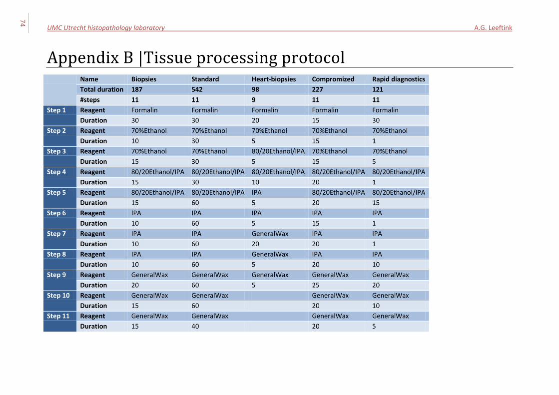
UMC Utrecht histopathology laboratory A.G. Leeftink
74
Appendix B |Tissue processing protocol Name Biopsies Standard Heart-biopsies Compromized Rapid diagnostics
Total duration 187 542 98 227 121
#steps 11 11 9 11 11
Step 1 Reagent Formalin Formalin Formalin Formalin Formalin
Duration 30 30 20 15 30
Step 2 Reagent 70%Ethanol 70%Ethanol 70%Ethanol 70%Ethanol 70%Ethanol
Duration 10 30 5 15 1
Step 3 Reagent 70%Ethanol 70%Ethanol 80/20Ethanol/IPA 70%Ethanol 70%Ethanol
Duration 15 30 5 15 5
Step 4 Reagent 80/20Ethanol/IPA 80/20Ethanol/IPA 80/20Ethanol/IPA 80/20Ethanol/IPA 80/20Ethanol/IPA
Duration 15 30 10 20 1
Step 5 Reagent 80/20Ethanol/IPA 80/20Ethanol/IPA IPA 80/20Ethanol/IPA 80/20Ethanol/IPA
Duration 15 60 5 20 15
Step 6 Reagent IPA IPA IPA IPA IPA
Duration 10 60 5 15 1
Step 7 Reagent IPA IPA GeneralWax IPA IPA
Duration 10 60 20 20 1
Step 8 Reagent IPA IPA GeneralWax IPA IPA
Duration 10 60 5 20 10
Step 9 Reagent GeneralWax GeneralWax GeneralWax GeneralWax GeneralWax
Duration 20 60 5 25 20
Step 10 Reagent GeneralWax GeneralWax GeneralWax GeneralWax
Duration 15 60 20 10
Step 11 Reagent GeneralWax GeneralWax GeneralWax GeneralWax
Duration 15 40 20 5
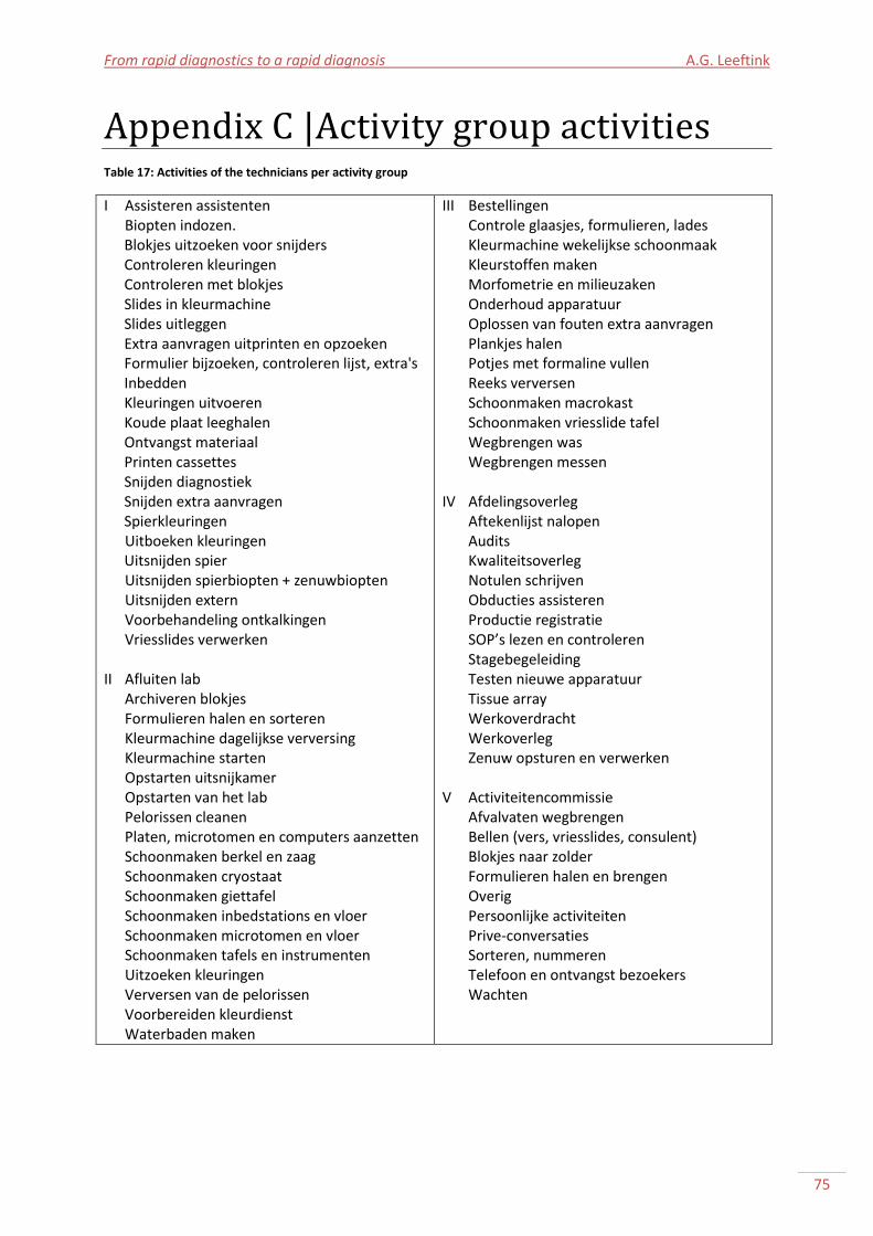
From rapid diagnostics to a rapid diagnosis A.G. Leeftink
75
Appendix C |Activity group activities Table 17: Activities of the technicians per activity group
I Assisteren assistenten Biopten indozen. Blokjes uitzoeken voor snijders Controleren kleuringen Controleren met blokjes Slides in kleurmachine Slides uitleggen Extra aanvragen uitprinten en opzoeken Formulier bijzoeken, controleren lijst, extra's Inbedden Kleuringen uitvoeren Koude plaat leeghalen Ontvangst materiaal Printen cassettes Snijden diagnostiek Snijden extra aanvragen Spierkleuringen Uitboeken kleuringen Uitsnijden spier Uitsnijden spierbiopten + zenuwbiopten Uitsnijden extern Voorbehandeling ontkalkingen Vriesslides verwerken II Afluiten lab Archiveren blokjes Formulieren halen en sorteren Kleurmachine dagelijkse verversing Kleurmachine starten Opstarten uitsnijkamer Opstarten van het lab Pelorissen cleanen Platen, microtomen en computers aanzetten Schoonmaken berkel en zaag Schoonmaken cryostaat Schoonmaken giettafel Schoonmaken inbedstations en vloer Schoonmaken microtomen en vloer Schoonmaken tafels en instrumenten Uitzoeken kleuringen Verversen van de pelorissen Voorbereiden kleurdienst Waterbaden maken
III Bestellingen Controle glaasjes, formulieren, lades Kleurmachine wekelijkse schoonmaak Kleurstoffen maken Morfometrie en milieuzaken Onderhoud apparatuur Oplossen van fouten extra aanvragen Plankjes halen Potjes met formaline vullen Reeks verversen Schoonmaken macrokast Schoonmaken vriesslide tafel Wegbrengen was Wegbrengen messen IV Afdelingsoverleg Aftekenlijst nalopen Audits Kwaliteitsoverleg Notulen schrijven Obducties assisteren Productie registratie SOP’s lezen en controleren Stagebegeleiding Testen nieuwe apparatuur Tissue array Werkoverdracht Werkoverleg Zenuw opsturen en verwerken V Activiteitencommissie Afvalvaten wegbrengen Bellen (vers, vriesslides, consulent) Blokjes naar zolder Formulieren halen en brengen Overig Persoonlijke activiteiten Prive-conversaties Sorteren, nummeren Telefoon en ontvangst bezoekers Wachten
UMC Utrecht histopathology laboratory A.G. Leeftink
76
Appendix D |Datasets The datasets consist of the scenario-dependent sets and parameters as given in Chapter 4. For each set and parameter, we will discuss how the values are derived and assigned.
Sets I I is the maximum number of orders arrived at the corresponding day, based on LMS data. Ij All large orders can be processed by resources 1, 6, …, 13 All small orders can be processed by resources 2, 5, …, 13 All priority orders can be processed by resources 2, …, 13 All external orders can be processed by resources 2, 4, …, 13 Jis Combination of Js and Ij NCis Empty sets for stages 2, 3, and 4. For stage 1, NCi1 consist of all large or non-large orders
respectively if the order i is non-large or large.
Parameters nsis For all orders, this equals s+1, since we consider the problem as a flow shop. s For all orders, this equals 4 ORTi For non-large specimens the release time of order i equals the timestamp. If no timestamp is
known, the time of registration in LMS is used. Since large specimens need fixation before grossing, these specimens always arrive at 7:30 AM.
di The due date of an order equals the release time plus a fixed time. For large orders 2880 minutes, for small orders 1800 minutes, for priority orders 300 minutes if arrived before 11:00 AM, or 1080 minutes if arrived after 11:00 AM, and for external specimens 1440 minutes.
tij The processing time is derived from the average processing time of the order (per cassette, per slide, etc, dependent of the stage) on the specific resource, derived from LMS.
ttij For all orders, between stage 1 and 2: 0 minutes. Between stage 2 and 3: 0 minutes. Between stage 3 and 4: 15 minutes for cooling purposes.
fij Depends on the stage of resource j. If stage 1: number of cassettes. If stage 2: 1. If stage 3: Number of molds. If stage 4: number of slides. Data is derived from the order data in LMS.
pi For large orders: 1, for small orders: 2, for external orders: 3, for priority orders: 4. Chosen in collaboration with lab manager, based on importance of timely examination of the specimen.
From rapid diagnostics to a rapid diagnosis A.G. Leeftink
77
Appendix E |Base scenario The base scenario consists of the sets and parameters which are fixed during all experiments, as given in Chapter 4.
Sets J {1, …, 13} S {1, …, 4} G {large, small, priority, external} B {1, …, 12} A {1, 2} Js J1 {1,2}, J2 {3, …, 6}, J3 {7,8}, and J4 {9, …, 13} Jbatch {3, …, 6} Jnon-batch {1, 2, 7, …, 13} Sbatch {2}
Parameters tbij Resource 3: 121 minutes, resource 4: 187 minutes, resource 5: 227 minutes, resource 6: 542
minutes, corresponding with the different protocols, as shown in Appendix B. URTj Equals the starting time of the staff member corresponding to the resource. bsjb bsj,1 = 1020, bsj,2 = 2460, bsj,3 = 3900 for j=4,5,6, bs3,1 = 675, bs3,2 = 1020, bs3,3 =2115, bs3,4
=2460, bs3,5 = 3555, and bs3,6 =3900. NW1aj For all a, equals the end time of the shift of the staff member corresponding to the resource. NW2a For all a: 1440. (Midnight) H 4320 minutes, which is 2 nights and 3 workdays. M 4320 minutes. Equals the planning horizon.
UMC Utrecht histopathology laboratory A.G. Leeftink
78
Appendix F |Past-processing algorithm The past-processing algorithm to reschedule order sequences is:
//initialize ordertime and resourcetime, with ordertime(i) = first available moment for order i and resourcetime(j) = first available moment on resource j OrderTime(i) := OrderReleaseTime(i); ResourceTime(j) := ResourceReleaseTime(j); //For each resource, assign orders in sequence such that orders are processed on their earliest //available processing time possible. FOR ((j,s)|j in ResourceSet(s)) DO TempOrder := 0; OldTempOrder := 0; //find 1st order scheduled on resource j, and reschedule this order to the 1st possible moment FOR (i|FirstOrder(i,j)=1) DO TempOrder := i; OrderTiming(i,s) := Max(OrderTime(i), ResourceTime(j)); Check break times; //reschedule order to determined time ResourceTime(j) := OrderTiming(i,s) + OrderFactor(i,j)*ProcessingTime(i,j);
OrderTime(i) := OrderTiming(i,s) + OrderFactor(i,j)*ProcessingTime(i,j) + TransferTime(i,s);
ENDFOR; WHILE TempOrder > 0 DO OldTempOrder := TempOrder; //find next order, and reschedule this order to the first possible moment FOR (i| OrderSequencing(TempOrder,i,s)=1) DO OrderTiming(i,s) := Max(OrderTime(i), ResourceTime(j)); Check break times;
ResourceTime(j) :=OrderTiming(i,s) + OrderFactor(i,j)*ProcessingTime(i,j);
OrderTime(i) :=OrderTiming(i,s) + OrderFactor(i,j)*ProcessingTime(i,j) + TransferTime(i,s);
TempOrder := i; ENDFOR; //if no order successor is found, quit while-statement IF (TempOrder = OldTempOrder) THEN TempOrder := 0; ENDIF; ENDWHILE; ENDFOR; DetermineDelay;
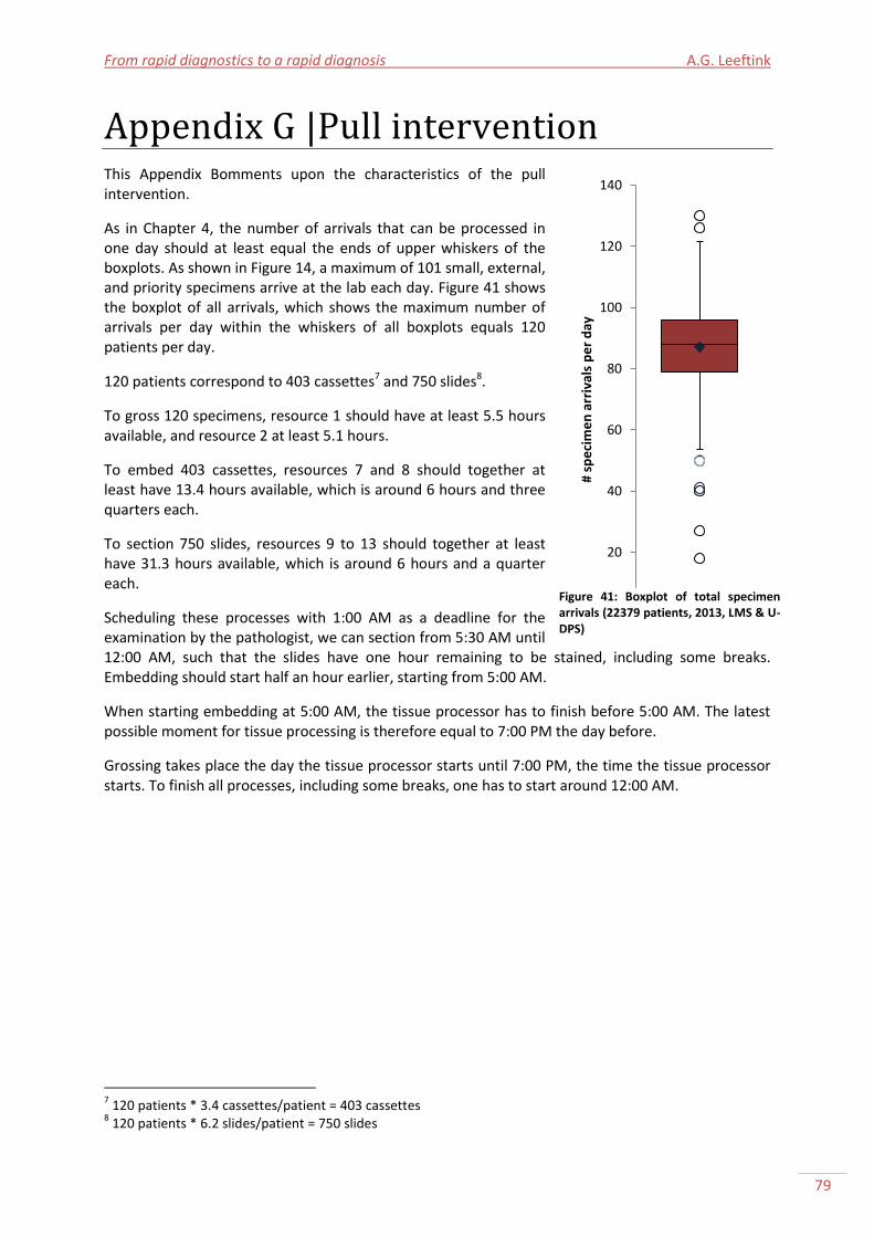
From rapid diagnostics to a rapid diagnosis A.G. Leeftink
79
Appendix G |Pull intervention This Appendix Bomments upon the characteristics of the pull intervention.
As in Chapter 4, the number of arrivals that can be processed in one day should at least equal the ends of upper whiskers of the boxplots. As shown in Figure 14, a maximum of 101 small, external, and priority specimens arrive at the lab each day. Figure 41 shows the boxplot of all arrivals, which shows the maximum number of arrivals per day within the whiskers of all boxplots equals 120 patients per day.
120 patients correspond to 403 cassettes7 and 750 slides8.
To gross 120 specimens, resource 1 should have at least 5.5 hours available, and resource 2 at least 5.1 hours.
To embed 403 cassettes, resources 7 and 8 should together at least have 13.4 hours available, which is around 6 hours and three quarters each.
To section 750 slides, resources 9 to 13 should together at least have 31.3 hours available, which is around 6 hours and a quarter each.
Scheduling these processes with 1:00 AM as a deadline for the examination by the pathologist, we can section from 5:30 AM until 12:00 AM, such that the slides have one hour remaining to be stained, including some breaks. Embedding should start half an hour earlier, starting from 5:00 AM.
When starting embedding at 5:00 AM, the tissue processor has to finish before 5:00 AM. The latest possible moment for tissue processing is therefore equal to 7:00 PM the day before.
Grossing takes place the day the tissue processor starts until 7:00 PM, the time the tissue processor starts. To finish all processes, including some breaks, one has to start around 12:00 AM.
7 120 patients * 3.4 cassettes/patient = 403 cassettes
8 120 patients * 6.2 slides/patient = 750 slides
0
20
40
60
80
100
120
140
# sp
eci
me
n a
rriv
als
pe
r d
ay
Figure 41: Boxplot of total specimen arrivals (22379 patients, 2013, LMS & U-DPS)
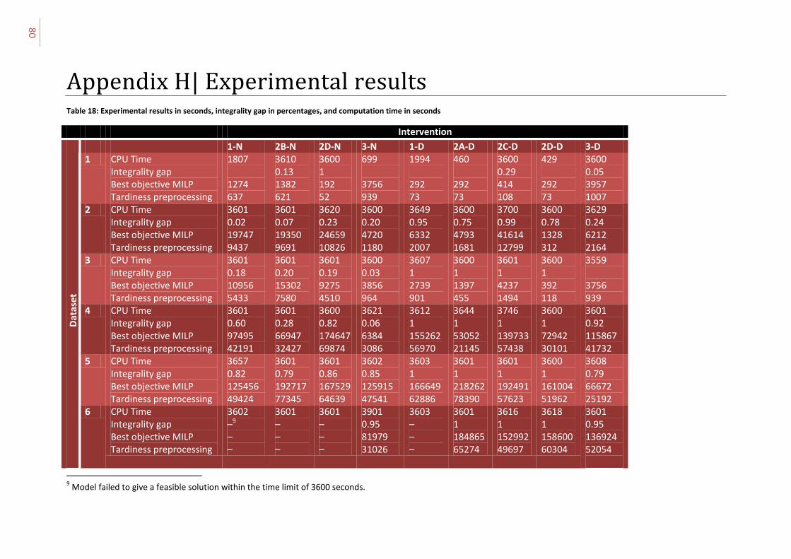
80
Appendix H| Experimental results Table 18: Experimental results in seconds, integrality gap in percentages, and computation time in seconds
Intervention
1-N 2B-N 2D-N 3-N 1-D 2A-D 2C-D 2D-D 3-D
Dat
ase
t
1 CPU Time Integrality gap Best objective MILP Tardiness preprocessing
1807 1274 637
3610 0.13 1382 621
3600 1 192 52
699 3756 939
1994 292 73
460 292 73
3600 0.29 414 108
429 292 73
3600 0.05 3957 1007
2 CPU Time Integrality gap Best objective MILP Tardiness preprocessing
3601 0.02 19747 9437
3601 0.07 19350 9691
3620 0.23 24659 10826
3600 0.20 4720 1180
3649 0.95 6332 2007
3600 0.75 4793 1681
3700 0.99 41614 12799
3600 0.78 1328 312
3629 0.24 6212 2164
3 CPU Time Integrality gap Best objective MILP Tardiness preprocessing
3601 0.18 10956 5433
3601 0.20 15302 7580
3601 0.19 9275 4510
3600 0.03 3856 964
3607 1 2739 901
3600 1 1397 455
3601 1 4237 1494
3600 1 392 118
3559 3756 939
4 CPU Time Integrality gap Best objective MILP Tardiness preprocessing
3601 0.60 97495 42191
3601 0.28 66947 32427
3600 0.82 174647 69874
3621 0.06 6384 3086
3612 1 155262 56970
3644 1 53052 21145
3746 1 139733 57438
3600 1 72942 30101
3601 0.92 115867 41732
5 CPU Time Integrality gap Best objective MILP Tardiness preprocessing
3657 0.82 125456 49424
3601 0.79 192717 77345
3601 0.86 167529 64639
3602 0.85 125915 47541
3603 1 166649 62886
3601 1 218262 78390
3601 1 192491 57623
3600 1 161004 51962
3608 0.79 66672 25192
6 CPU Time Integrality gap Best objective MILP Tardiness preprocessing
3602 –9 – –
3601 – – –
3601 – – –
3901 0.95 81979 31026
3603 – – –
3601 1 184865 65274
3616 1 152992 49697
3618 1 158600 60304
3601 0.95 136924 52054
9 Model failed to give a feasible solution within the time limit of 3600 seconds.
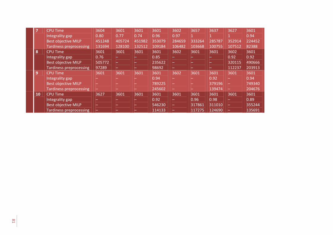
81
7 CPU Time Integrality gap Best objective MILP Tardiness preprocessing
3604 0.80 451248 131694
3601 0.77 405724 128100
3601 0.74 451982 132512
3601 0.96 353079 109184
3602 0.97 284659 106482
3657 1 333264 103668
3637 1 285787 100755
3627 1 352914 107512
3601 0.94 224452 82388
8 CPU Time Integrality gap Best objective MILP Tardiness preprocessing
3601 0.76 505772 97289
3601 – – –
3601 – – –
3601 0.85 235622 98692
3602 – – –
3601 – – –
3601 – – –
3602 0.92 320115 112237
3601 0.92 490666 203913
9 CPU Time Integrality gap Best objective MILP Tardiness preprocessing
3601 – – –
3601 – – –
3601 – – –
3601 0.94 789225 245602
3602 – – –
3601 – – –
3601 0.92 379196 139474
3601 – – –
3601 0.94 749340 204676
10 CPU Time Integrality gap Best objective MILP Tardiness preprocessing
3627 – – –
3601 – – –
3601 – – –
3601 0.92 546230 114133
3601 – – –
3601 0.96 317861 117275
3601 0.98 311010 124690
3601 – – –
3601 0.89 355244 135691
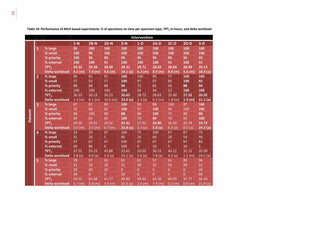
82
Table 19: Performance of MILP-based experiments: % of specimens on time per specimen type, TPT2 in hours, and delta workload
Intervention
1-N 2B-N 2D-N 3-N 1-D 2A-D 2C-D 2D-D 3-D
Dat
ase
t
1 % large % small % priority % external TPT2 Delta workload
95 100 100 100 29.22 4.5 (m)
100 96 95 100 29.38 7.0 (m)
100 100 90 91 28.49 9.6 (m)
100 100 95 100 28.31 19.1 (a)
100 100 95 100 29.71 6.3 (m)
100 100 95 100 28.02 8.9 (m)
100 100 90 91 28.04 8.8 (m)
100 100 95 100 28.90 5.6 (m)
100 100 95 91 29.13 18.0 (a)
2 % large % small % priority % external TPT2 Delta workload
95 57 88 100 30.33 1.3 (m)
91 53 88 100 30.13 8.1 (m)
91 57 88 100 30.23 10.6 (m)
100 100 94 100 26.63 23.0 (a)
100 97 75 56 28.73 2.3 (a)
95 97 81 44 28.63 0.2 (m)
77 83 56 22 35.40 1.8 (m)
100 100 88 100 27.52 1.9 (m)
100 93 94 100 26.92 21.5 (a)
3 % large % small % priority % external TPT2 Delta workload
87 76 88 85 29.10 5.0 (m)
87 68 100 65 29.31 2.5 (m)
80 82 88 85 29.32 6.7 (m)
100 100 88 100 25.41 25.8 (a)
93 97 88 70 27.92 2.3 (a)
93 100 100 80 26.80 5.8 (a)
100 94 75 70 26.50 6.3 (a)
87 100 88 95 26.79 0.5 (a)
100 100 88 100 24.72 24.2 (a)
4 % large % small % priority % external TPT2 Delta workload
33 31 67 60 37.52 5.8 (a)
33 26 67 80 33.15 4.0 (a)
67 5 67 0 45.88 2.4 (a)
100 85 100 100 23.65 23.1 (a)
75 26 67 0 10.03 5.6 (a)
100 69 67 10 30.15 7.8 (a)
67 26 67 5 40.22 4.3 (a)
67 54 67 30 32.15 1.5 (m)
75 46 83 5 35.99 24.5 (a)
5 % large % small % priority % external TPT2 Delta workload
78 31 20 48 39.55 5.7 (m)
57 18 40 0 41.68 3.8 (m)
65 28 20 9 41.77 3.4 (m)
61 31 0 50 40.89 25.6 (a)
61 38 0 0 39.63 2.0 (m)
57 33 0 0 42.50 7.4 (m)
61 54 0 5 40.03 0.2 (m)
83 49 0 0 37.77 0.9 (m)
96 51 20 68 36.33 21.9 (a)
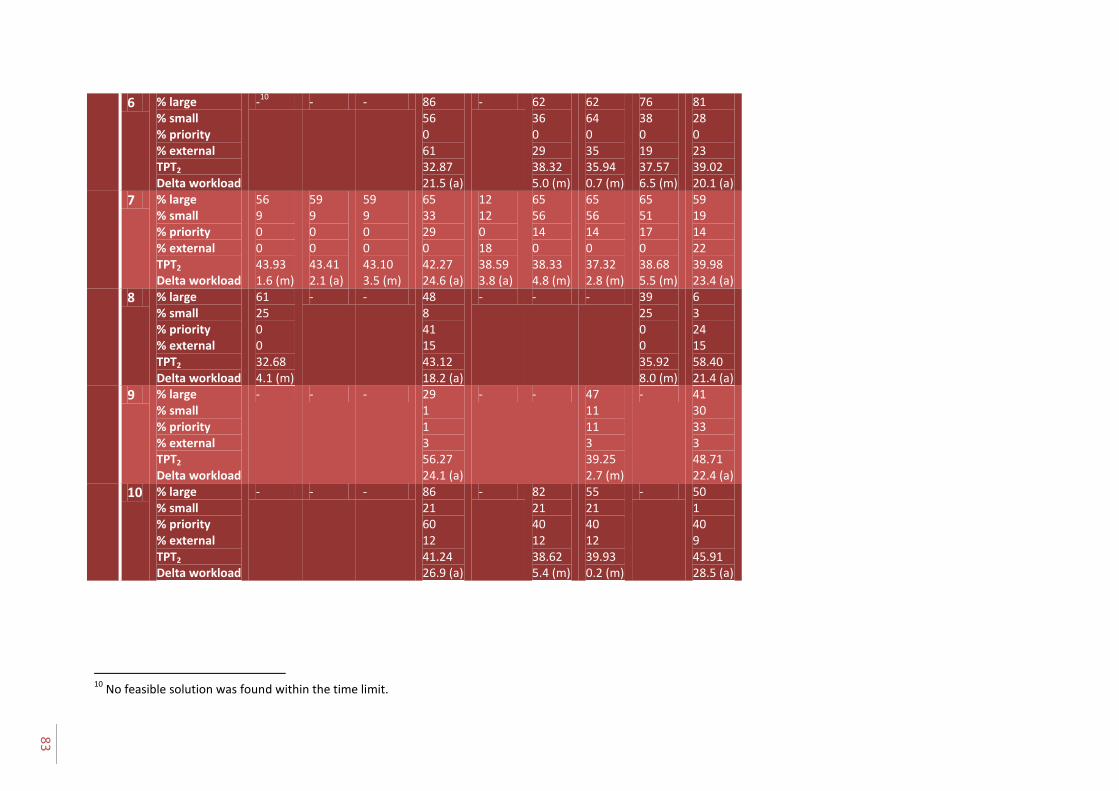
83
6 % large % small % priority % external TPT2 Delta workload
-10
- - 86 56 0 61 32.87 21.5 (a)
- 62 36 0 29 38.32 5.0 (m)
62 64 0 35 35.94 0.7 (m)
76 38 0 19 37.57 6.5 (m)
81 28 0 23 39.02 20.1 (a)
7 % large % small % priority % external TPT2 Delta workload
56 9 0 0 43.93 1.6 (m)
59 9 0 0 43.41 2.1 (a)
59 9 0 0 43.10 3.5 (m)
65 33 29 0 42.27 24.6 (a)
12 12 0 18 38.59 3.8 (a)
65 56 14 0 38.33 4.8 (m)
65 56 14 0 37.32 2.8 (m)
65 51 17 0 38.68 5.5 (m)
59 19 14 22 39.98 23.4 (a)
8 % large % small % priority % external TPT2 Delta workload
61 25 0 0 32.68 4.1 (m)
- - 48 8 41 15 43.12 18.2 (a)
- - - 39 25 0 0 35.92 8.0 (m)
6 3 24 15 58.40 21.4 (a)
9 % large % small % priority % external TPT2 Delta workload
- - - 29 1 1 3 56.27 24.1 (a)
- - 47 11 11 3 39.25 2.7 (m)
- 41 30 33 3 48.71 22.4 (a)
10 % large % small % priority % external TPT2 Delta workload
- - - 86 21 60 12 41.24 26.9 (a)
- 82 21 40 12 38.62 5.4 (m)
55 21 40 12 39.93 0.2 (m)
- 50 1 40 9 45.91 28.5 (a)
10
No feasible solution was found within the time limit.

UMC Utrecht histopathology laboratory A.G. Leeftink
84
Appendix I |Statistical analyses Verification statistics – Base scenario We will formally check the fit between the modeled performance (frequency distribution of success (examination on time)) and our theoretical distribution of performance, derived from historical data. Therefore, we perform a test of goodness of fit by means of a Chi-square test, which is suitable since the population is more than 10 times larger than the sample data and each variable has an expected frequency count of at least 5 orders examined on time. We show the steps for the chi-squared test applied to the distribution of performance of large specimens.
1. Independent variables Xon time, Xnot on time are distributed with chances pon time, pnot on time, according to the distribution of performance of the model for each specimen type.
2. Hypothesis H0: pi = p0i for all specimen types, with i {on time, not on time}
3. , with Oi = observed frequency, Ei = expected frequency.
4. Chi-square has under H0 a chi-square-distribution with n=1 degrees of freedom. 5. Alhpa = 0,05 6. The value of Chi-square = 4.94. 7. The critical area is [3.84, inf). 8. 4.94 > 3,84. Chi-square is in the critical area, and therefore H0 is rejected. 9. Conclusion: There is a significant difference in the distribution of the modeled performance
compared to the theoretical performance.
For small specimens, no statistical differences were found in the modeled performance compared to the historical data (chi-square = 0,04, df=1, p>0,05). For external specimens, a significant difference was found (chi-square – 4,98, df=1, p<0,05).
For priority specimens, the expected frequency count of specimens not examined on time equals 3,6. This is lower than 5, which is the minimum expected frequency count needed for a reliable chi-square test. Therefore, we cannot say anything on the statistical significance of the modeled performance of priority specimens.
Performance statistics - Current situation We checked the significance of the difference in performance of the base scenario without tissue processing during the day against the performance of the base scenario with tissue processing during the day by performing a paired t-test, since both performances were derived based on the same datasets. We compared the configurations on TPT2. n and m are both 10 observations. We construct a confidence interval for .
1. Xj and Yj are independent observations, for i = 1,...,10 and j = 1,…,10. 2. H0: Difference in TPT2 times = 0
Ha: Difference in TPT2 times ≠ 0 3. We perform a paired-t test and we use the t-distribution, with
, with
4. Given H0, t is t-distributed, with n-1 = 9 degrees of freedom. 5. Alpha = 0,05 6. t = t9, 0,975 = 2,26 7. The critical area is (3,48, 7,13) 8. The value of T = 0.
From rapid diagnostics to a rapid diagnosis A.G. Leeftink
85
9. T is not in the critical area, and therefore H0 is rejected with a significance of alpha = 0,05.
We have statistically shown that the performance of the base scenario with and without tissue processing during the day have different performances.
Performance statistics - Pull situation We checked the significance of the difference in performance of the pull interventions without tissue processing during the day against the performance of the pull intervention with tissue processing during the day by performing a paired t-test, since both performances were derived based on the same datasets. We compared the configurations on TPT2. n and m are both 10 observations. We construct a confidence interval for .
1. Xj and Yj are independent observations, for i = 1,...,10 and j = 1,…,10. 2. H0: Difference in TPT2 times = 0
Ha: Difference in TPT2 times ≠ 0 3. We perform a paired-t test and we use the t-distribution, with
, with
4. Given H0, t is t-distributed, with n-1 = 9 degrees of freedom. 5. Alpha = 0,05 6. t = t9, 0,975 = 2,26 7. The critical area is (-0,26, 0,07) 8. The value of T = 0. 9. T is in the critical area, and therefore H0 is accepted with a significance of alpha = 0,05.
We have no statistical evidence that the performance of the pull interventions with and without tissue processing during the day have different performances.