frequency– and pressure – dependent dynamic soil properties for
TRANSCRIPT

FREQUENCY– AND PRESSURE – DEPENDENT DYNAMIC SOIL PROPERTIES FOR THE SEISMIC ANALYSIS OF DEEP SITES
ASSIMAKI, Dominic
MSc, Graduate Research Fellow, National Technical University of Athens, Geotechnical Division, 42 Patission str. , 10682 Athens, GREECE, [email protected]
KAUSEL, Eduardo
Professor MIT, Massachusetts Institute of Technology, Rm. 1-239, 77 Massachusetts Av., Cambridge MA02139,
USA, [email protected]
ABSTRACT The numerical models most often used to assess the response of soil deposits to strong earthquake motions are typically based on the assumptions of quasi-linear elastic, small-strain behavior cast in the context of an iterative computational scheme. The seismic analysis of soil deposits is most often carried out with an iterative computational scheme first proposed by Seed & Idriss, 1969. Laboratory experimental data (Laird & Stokoe, 1993), performed on sand samples subjected to high confining pressures, show that for highly confined materials, both the standard shear modulus reduction factor [G /G 0] and damping [ξ ] versus shear strain amplitude, overestimate the capacity of soil to dissipate energy. On the other hand, the iterative linear algorithm may also diverge when soil amplification is performed in deep soft soil profiles, due to the assumption of a linear hysteretic damping being independent of frequency. This paper first presents a simple four-parameter constitutive soil model, derived from Pestana's (1994) MIT-S1 generalized effective stress formulation. When used to simulate sand behavior under both small and large confining pressures, subjected to cyclic shear tests, results are found to be in very good agreement with available laboratory experimental data. Thereafter, simulations for a series of “true” non-linear numerical analyses with inelastic (Masing-type) soils and layered profiles subjected to broadband earthquake motions, taking into account the effect of the confining pressure, are presented. It is found that the actual inelastic behavior can be closely simulated by means of equivalent linear analyses, in which the soil moduli and damping are frequency– and pressure– dependent. Using a modified linear iterative analysis with frequency- and depth-dependent moduli and attenuation, a 1-km deep model for the Mississippi embayment near Memphis, Tennessee, is successfully analyzed. Keywords: Soil dynamics, seismic wave amplification, effective stress soil model, elastodynamics, inelastic soil behavior, deep soil profile, SHAKE.
INTRODUCTION Assessments of seismic effects in soil deposits are now routinely made taking into account inelastic soil behavior, and most often this is done with an iterative scheme first proposed by Seed and Idriss (1969). In this method, approximate linear solutions are obtained by assuming depth-dependent values for shear moduli and damping that remain constant for the duration of the earthquake simulation. These properties are chosen at the beginning of each iteration so as to be consistent with the levels of strain computed in the previous iteration. While the iterative linear algorithm often provides acceptable results for engineering purposes, it has a number of shortcomings, of which the most important are: • When the seismic excitation is prescribed at or near the surface of a deep deposit of soft soil, the model may
diverge if the specified motion is either too large in amplitude or too rich in high frequencies. This is because when motions are deconvolved to bedrock, they must grow exponentially with depth to overcome the attenuation. Damping in turn grows from iteration to iteration because motions grow more intense.
2
0
0.4
0.8
1.2
10-6 10-5 10-4 10-3
Seed & Idriss (1970)
Experimental Data onDry Remolded Sand σ ' [kPa] = 25 ÷ 2000
Cyclic Shear Strain [γc ]
G /
Gm
ax
0.02
0.04
0.06
0.08
0.10
10-6 10-5 10-4 10-3
Seed & Idriss (1970)
Experimental Data onDry Remolded Sand σ ' [kPa] = 25 ÷ 2000
Cyclic Shear Strain [ γc
]
Mat
eria
l Dam
ping
ξ
The excitation specified at the free surface is then inconsistent with the linear model used, particularly because damping is assumed to remain constant with frequency.
• Conversely, when the excitation is prescribed at the base of a deep, soft soil deposit (or at some hypothetical
outcropping of rock), the iterations do converge, but the spectra for motions obtained near the free surface have unrealistically low values at high frequencies (say, above 3 Hz). Again, this is the result of a model in which damping remains constant with frequency, and thus wipes out the high end of the output spectrum.
Clearly, the adoption of a frequency-independent linear hysteretic model to simulate what is an intrinsically non-linear process is only an approximation. Since material damping is a function of amplitude, high frequencies associated with small amplitude cycles of vibration must have substantially less damping than the predominant frequencies of the excitation. This issue is taken up in this paper, where an improved version of the Seed-Idriss iterative linear model is presented, which takes into account the frequency- and amplitude-dependent nature of the material parameters. The proposed scheme not only provides results that match more closely the inelastic behavior of soils undergoing seismic deformations in shear, but it does so without substantially adding complexity to the iterative algorithm.
EFFECT OF CONFINING PRESSURE ON MODULUS AND DAMPING
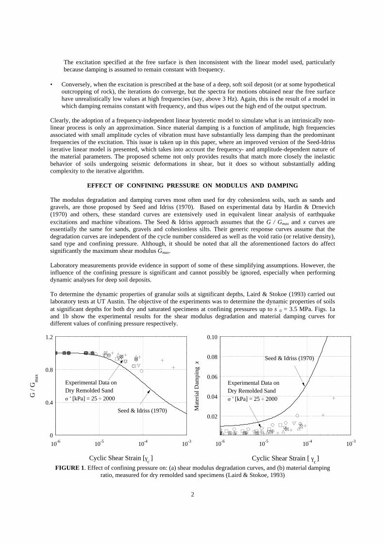
The modulus degradation and damping curves most often used for dry cohesionless soils, such as sands and gravels, are those proposed by Seed and Idriss (1970). Based on experimental data by Hardin & Drnevich (1970) and others, these standard curves are extensively used in equivalent linear analysis of earthquake excitations and machine vibrations. The Seed & Idriss approach assumes that the G / Gmax and ξ curves are essentially the same for sands, gravels and cohesionless silts. Their generic response curves assume that the degradation curves are independent of the cycle number considered as well as the void ratio (or relative density), sand type and confining pressure. Although, it should be noted that all the aforementioned factors do affect significantly the maximum shear modulus Gmax. Laboratory measurements provide evidence in support of some of these simplifying assumptions. However, the influence of the confining pressure is significant and cannot possibly be ignored, especially when performing dynamic analyses for deep soil deposits.
To determine the dynamic properties of granular soils at significant depths, Laird & Stokoe (1993) carried out laboratory tests at UT Austin. The objective of the experiments was to determine the dynamic properties of soils at significant depths for both dry and saturated specimens at confining pressures up to σ’
0 = 3.5 MPa. Figs. 1a and 1b show the experimental results for the shear modulus degradation and material damping curves for different values of confining pressure respectively.
FIGURE 1. Effect of confining pressure on: (a) shear modulus degradation curves, and (b) material damping ratio, measured for dry remolded sand specimens (Laird & Stokoe, 1993)

3
As it can be readily seen, the soil stress-strain response becomes more linear as the confining pressure increases (i.e. as σ’
0 increases, G / Gmax increases and ξ decreases). In addition, large confining pressures lead to substantial reductions in material damping at small strain, i.e. ξ min. The reason for these effects with increasing σ’
0 is related to the different rates at which the small strain modulus and the shear strength of the soil increase when the pressure increases (Hardin & Drnevich, 1972a, Seed et al., 1986, Laird & Stokoe, 1993). The need to implement concisely the experimental results presented previously into a computer code for seismic amplification provided the motivation for formulating a theoretical model representing the effect of confining pressure on the soil behavior under cyclic loading.
MIT-S1 MODEL FOR SANDS AND CLAYS
Pestana (1994) developed a generalized, effective stress soil model, referred to as MIT-S1, which describes the rate independent behavior of freshly deposited and overconsolidated soils. The MIT-S1 model formulation is based on the incrementally linearized theory of rate-independent elastoplasticity. Provided that modulus degradation and damping for 1-D wave propagation problems involve relatively small strain amplitudes (i.e. plastic components of deformation can be ignored), a reduced form of the MIT-S1 model was used to model the behavior of granular materials under cyclic shear and constant effective stress. In the resulting simple four-parameter model, analytical expressions were derived for the shear modulus degradation and damping ratio curves in which, the effect of confining pressure, is explicitly taken into account in the soil stiffness. Figs. 2a and 2b show a comparison between the shear modulus reduction and damping curves respectively, predicted by the proposed formulation and the experimental data presented by Laird & Stokoe (1993). Results are found to be in very good agreement for all tests with σ’
0 = 28 to 1800 kPa.
FIGURE 2. (a) Shear modulus degradation, and (b) damping vs. cyclic strain amplitude for different levels of
confining pressure, MIT-S1 model vs. experimental data.
0
0.4
0.8
1.2
10-6 10-5 10-4 10-3
1766 kPa, e = 0.636
883 kPa, e = 0.646
442 kPa, e = 0.653
221 kPa, e = 0.658
110 kPa, e = 0.661
55.2 kPa, e = 0.662
27.6 kPa, e = 0.663
MIT-S1 model predictions
Cyclic Shear Strain [ γc ]
G /
Gm
axG
/ G
max
0.02
0.04
0.06
0.08
0.10
10-6 10-5 10-4 10-3
1766 kPa, e = 0.636
883 kPa, e = 0.646
442 kPa, e = 0.653
221 kPa, e = 0.658
110 kPa, e = 0.661
55.2 kPa, e = 0.662
27.6 kPa, e = 0.663
MIT-S1 model predictions
Cyclic Shear Strain [ γc
]
Mat
eria
l Dam
ping
ξM
ater
ial D
ampi
ng ξ
4
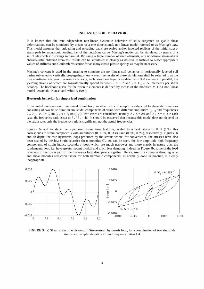
INELASTIC SOIL BEHAVIOR It is known that the rate-independent non-linear hysteretic behavior of soils subjected to cyclic shear deformations, can be simulated by means of a one-dimensional, non-linear model referred to as Masing’s law. This model assumes that unloading and reloading paths are scaled and/or inverted replicas of the initial stress-strain path for monotonic loading, i.e. of the backbone curve. Masing’s model can be simulated by means of a set of elasto-plastic springs in parallel. By using a large number of such elements, any non-linear stress-strain characteristic obtained from test results can be simulated as closely as desired. It suffices to select appropriate values of stiffness and Coulomb resistance for as many elasto-plastic springs as may be necessary Masing’s concept is used in the ensuing to simulate the non-linear soil behavior in horizontally layered soil basins subjected to vertically propagating shear waves; the results of these simulations shall be referred to as the true non-linear analyses. To ensure accuracy, each non-linear layer is modeled with 300 elements in parallel, the yielding strains of which are logarithmically spaced between ? = 10-6 and ? = 1 (i.e. 50 elements per strain decade). The backbone curve for the discrete elements is defined by means of the modified MIT-S1 non-linear model (Assimaki, Kausel and Whittle, 1999). Hysteretic behavior for simple load combination In an initial non-harmonic numerical simulation, an idealized soil sample is subjected to shear deformations consisting of two finite duration sinusoidal components of strain with different amplitudes ?1, ?2 and frequencies ? 1, ? 2 , i.e. ? = ?1 sin (? 1 t) + ?2 sin (? 2 t). Two cases are considered, namely ?1 / ?2 = 2:1 and ?1 / ?2 = 4:1; in each case, the frequency ratio is set to ? 1 / ? 2 = 4:1. It should be observed that because this model does not depend on the strain rate, only the frequency ratio is significant, not the actual frequencies. Figures 3a and 4a show the superposed strain time histories, scaled to a peak strain of 0.01 (1%); this corresponds to strain components with amplitudes (0.667%, 0.333%) and (0.8%, 0.2%), respectively. Figures 3b and 4b depict the true hysteresis loops produced by the strains where, for convenience, the stresses have also been scaled by the low-strain (elastic) shear modulus G0. As can be seen, the low-amplitude high-frequency components of strain induce secondary loops which are much narrower and more elastic in nature than the fundamental loop i.e. have greater secant moduli and much less damping. Indeed, in Figure 4b, some of the load reversals in the lower part of the hysteresis loop disappear altogether! Hence, use of a common damping ratio and shear modulus reduction factor for both harmonic components, as normally done in practice, is clearly inappropriate.
FIGURE 3. (a) Shear strain time history, (b) Stress–strain hysteresis loop, for a combination of two sinusoidal
strains with amplitude ratios 2:1 and frequency ratios 1:4.
-0.010
-0.005
0
0.005
0.010
0 0.2 0.4 0.6 0.8 1.0
-0.0010
-0.0005
0
0.0005
0.0010
-0.010 -0.005 0 0.005 0.010
G / G0 = 0.1895
G / G0 = 0.0708
Stre
ss [
τ ]
5
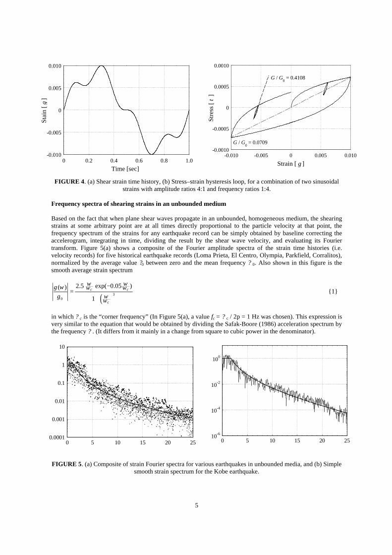
FIGURE 4. (a) Shear strain time history, (b) Stress–strain hysteresis loop, for a combination of two sinusoidal strains with amplitude ratios 4:1 and frequency ratios 1:4.
Frequency spectra of shearing strains in an unbounded medium Based on the fact that when plane shear waves propagate in an unbounded, homogeneous medium, the shearing strains at some arbitrary point are at all times directly proportional to the particle velocity at that point, the frequency spectrum of the strains for any earthquake record can be simply obtained by baseline correcting the accelerogram, integrating in time, dividing the result by the shear wave velocity, and evaluating its Fourier transform. Figure 5(a) shows a composite of the Fourier amplitude spectra of the strain time histories (i.e. velocity records) for five historical earthquake records (Loma Prieta, El Centro, Olympia, Parkfield, Corralitos), normalized by the average value ?0 between zero and the mean frequency ? 0. Also shown in this figure is the smooth average strain spectrum
( )30
2.5 exp( 0.05 )( )
1
ω ωω ω
ωω
γ ωγ
−=
+
c c
c
{1}
in which ? c is the “corner frequency” (In Figure 5(a), a value fc = ? c / 2p = 1 Hz was chosen). This expression is very similar to the equation that would be obtained by dividing the Safak-Boore (1986) acceleration spectrum by the frequency ? . (It differs from it mainly in a change from square to cubic power in the denominator).
FIGURE 5. (a) Composite of strain Fourier spectra for various earthquakes in unbounded media, and (b) Simple
smooth strain spectrum for the Kobe earthquake.
-0.010
-0.005
0
0.005
0.010
0 0.2 0.4 0.6 0.8 1.0Time [sec]
Stai
n [ γ
]
-0.0010
-0.0005
0
0.0005
0.0010
-0.010 -0.005 0 0.005 0.010
G / G0 = 0.4108
G / G0 = 0.0709
Strain [ γ ]
Stre
ss [
τ ]
0.0001
0.001
0.01
0.1
1
10
0 5 10 15 20 2510-6
10-4
10-2
100
0 5 10 15 20 25
6
As can be seen, the strain Fourier spectra for various earthquakes are very similar to each other. In all cases, the amplitudes of spectral strain do decay with frequency, and at 20 Hz, they have fallen by nearly three orders of magnitude. An even simpler smooth strain spectrum is shown in Figure 5(b), which is obtained by taking a constant value equal to the average Fourier amplitude in the range from zero to the mean frequency ? 0, and fitting an exponential expression after that, i.e.
( )
0
00
0
0
1( ) exp( )
β
ωω
ωω
ω ωγ ω α
ω ωγ
≤ −= >
{2}
This expression is convenient, because when its logarithm is taken, the two unknown parameters a, ß appear linearly. This in turn permits a simple least-squares optimal fit for a and ß (subjected to the subsidiary condition for a to be non-negative). The best-fit values used in Figure 5b for the Kobe earthquake are a = 0.2825 and ß = 2.222. Inasmuch as the strain spectra decay strongly with frequency, the high-frequency components must surely produce secondary hysteresis loops that are much more elastic than the primary loops elicited by the high-amplitude, low frequency components. Thus, it seems natural that, to match more closely to inelastic soil behavior with a linear hysteretic model, one must modify both the shear modulus and damping in accord with the spectral content of the strains.
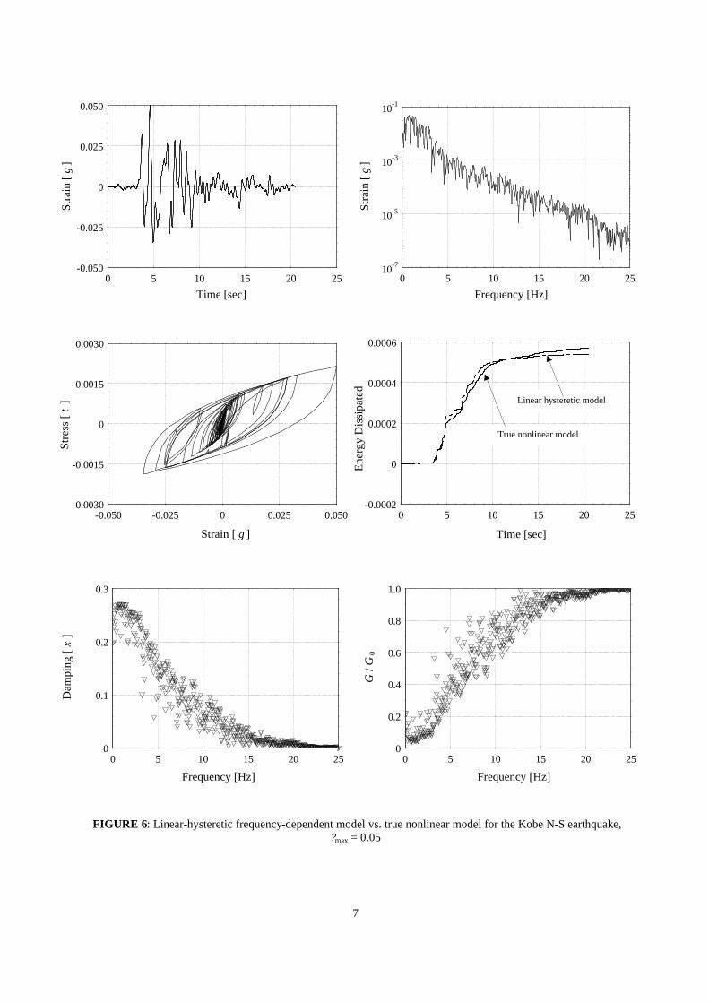
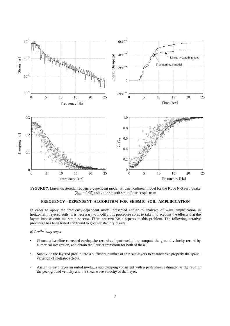
FREQUENCY DEPENDENT SHEAR MODULUS AND DAMPING The frequency-dependent model presented, is first demonstrated by means seismic waves propagating in an unbounded medium. For this purpose, simulations are carried out by subjecting the soil to strain time histories identical to the velocity records of actual earthquakes, but scaled to strain maxima large enough to produce clear inelastic effects. First, the velocity time history for an actual record is scaled and converted into a strain time history with some arbitrary peak strain ?0. The Fourier amplitude spectrum is next obtained and normalized so that its peak spectral amplitude equals the peak strain. At first, no attempts are made to smooth out the strain spectrum; instead, the ordinates are used directly to read out the shear modulus reduction factor and damping value for that particular frequency from curves such as those in Figure 2. These values are then used to evaluate the time histories for the elastic and dissipative components of the stress, and from here, the instantaneous power and dissipated energy. Figure 6a presents the strain time history for one of the 1995 Kobe records, scaled to maximum strains of 0.05. Figure 6b shows the true hysteresis loops, which illustrates very clearly the strong non-linear effects induced in the soil. Figure 6c-d depicts the frequency-dependent damping and the shear modulus reduction factor that are consistent with the spectral strain ordinates. As can be seen, above some 5 Hz, the soil rapidly recovers its full elastic values. Finally, Figure 6e shows a comparison between the true dissipated energy and the dissipated energy implied by the linear hysteretic model. The agreement between these two is rather remarkable, not only with respect to total energy dissipated, but also as to how this energy increases with time. A second simulation is then carried out with the smooth version of the strain spectrum given by equation 2 (i.e. Figure 5b), setting ?0 equal to the peak strain. Figure 7 shows the results of this model, organized in the same fashion as in Figure 6. The agreement in the time evolution of dissipated energy is still very good indeed. The advantage of using a smooth strain spectrum for wave propagation and iterative soil amplification analyses is that it leads to smooth variations of shear moduli and damping, which in turn leads to a more robust and stable algorithm.
7
FIGURE 6: Linear-hysteretic frequency-dependent model vs. true nonlinear model for the Kobe N-S earthquake,
?max = 0.05
Time [sec]
Stra
in [
γ ]
Stra
in [
γ ]
Frequency [Hz]
-0.050
-0.025
0
0.025
0.050
0 5 10 15 20 25
-0.0002
0
0.0002
0.0004
0.0006
0 5 10 15 20 25
Time [sec] Strain [ γ ]
Ene
rgy
Dis
sipa
ted
Stre
ss [
τ ]
True nonlinear model
Linear hysteretic model
-0.0030
-0.0015
0
0.0015
0.0030
-0.050 -0.025 0 0.025 0.050
Frequency [Hz] Frequency [Hz]
G /
G 0
Dam
ping
[ ξ
]
0
0.1
0.2
0.3
0 5 10 15 20 250
0.2
0.4
0.6
0.8
1.0
0 5 10 15 20 25
10-7
10-5
10-3
10-1
0 5 10 15 20 25
8
F?GURE 7. Linear-hysteretic frequency-dependent model vs. true nonlinear model for the Kobe N-S earthquake
(?max = 0.05) using the smooth strain Fourier spectrum
FREQUENCY – DEPENDENT ALGORITHM FOR SEISMIC SOIL AMPLIFICATION In order to apply the frequency-dependent model presented earlier to analyses of wave amplification in horizontally layered soils, it is necessary to modify this procedure so as to take into account the effects that the layers impose onto the strain spectra. There are two basic aspects to this problem. The following iterative procedure has been tested and found to give satisfactory results: a) Preliminary steps • Choose a baseline-corrected earthquake record as input excitation, compute the ground velocity record by
numerical integration, and obtain the Fourier transform for both of these. • Subdivide the layered profile into a sufficient number of thin sub-layers to characterize properly the spatial
variation of inelastic effects. • Assign to each layer an initial modulus and damping consistent with a peak strain estimated as the ratio of
the peak ground velocity and the shear wave velocity of that layer.
10-7
10-5
10-3
10-1
0 5 10 15 20 25
0
0.1
0.2
0.3
0 5 10 15 20 25
-2x10⁻⁴
0
2x10⁻⁴
4x10⁻⁴
6x10⁻⁴
0 5 10 15 20 25
Time [sec]
Ene
rgy
Dis
sipa
ted
True nonlinear model
Linear hysteretic model
Frequency [Hz]
Stra
in [
γ ]
Frequency [Hz]
Dam
ping
[ ξ
]
Frequency [Hz]
G /
G 0
0
0.2
0.4
0.6
0.8
1.0
0 5 10 15 20 25
9
b) Iterative algorithm • Using a standard wave amplification model (i.e. Haskell-Thompson), determine the transfer functions for
the strains at the center of each layer for a unit input velocity (not input acceleration!) specified at bedrock or rock outcrop. (This circumvents the problem of having to divide the acceleration transfer functions by the frequency, which produces uncertain results at low frequencies).
• Multiply each transfer function by the input velocity spectrum, Fourier-invert the result to obtain strain time
histories, and find the true peak strains ?0. • In each layer, determine the mean frequency ? 0 of the strain spectrum, and the least-squares best-fit
parameters a, ß? for the smooth strain spectrum given by equation 2. • Use the smooth spectrum curve thus obtained to extract the frequency-dependent soil parameters, i.e. the
shear modulus reduction factor and the fraction of damping. Modify the soil constants accordingly. • Compare the peak strains with their values in the previous iteration. Iterate as necessary. • After the convergence criterion is satisfied, compute the acceleration (or other) response time histories
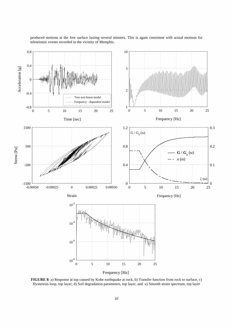
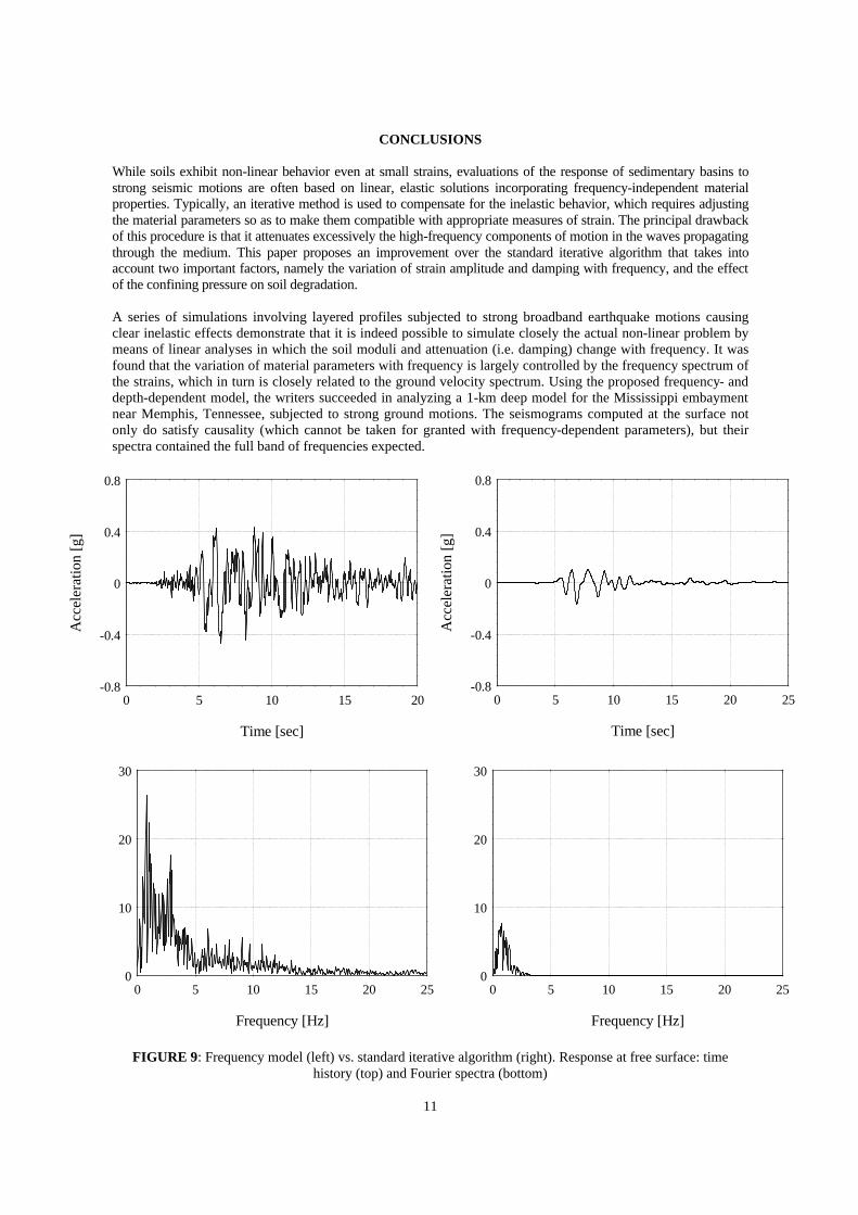
wherever desired. As can be seen, other than how the frequency-dependent moduli are found, this method agrees with the standard Seed-Idriss method. This algorithm is applied for the analysis of a 1-km deep model for the Mississippi embayment near Memphis, Tennessee, for which the response is computed both with the true non-linear model and with the frequency/confining-pressure dependent hysteretic model. Example: Deep, heterogeneous stratum An idealized soil profile of depth 1000m is used to simulate the Mississippi embayment near Memphis, Tennessee. The inelastic characteristics are chosen to be the same as for the remolded sand specimens of Laird & Stokoe (1993), taking into account the confining pressure. To this effect, the variation of void ratio with the mean effective stress is modeled with the original MIT-S1 formulation for cohesionless soils given by Pestana & Whittle (1995). This model is then used both to estimate the small strain (γ = 10-6) shear modulus Gmax and to determine the modulus degradation and damping curves. The mass density ranges from 2.12 ton/m3 at the surface to 2.21 ton/m3 near the rock interface. The shear wave velocity profile for the Memphis area used, is the one reported by Abrams & Shinozuka (1997). The soil profile is divided into 100 thin layers of 10m thickness. The model is subjected to the 1995 Kobe (Japan) earthquake, which is scaled to a maximum acceleration of 0.5g prescribed at a hypothetical outcropping of rock. The fundamental shear-beam frequency of this soil basin is 0.156 Hz, and there are some 70 (!) resonant modes in the 0-25 Hz frequency range. Because of this very low fundamental frequency as well as the large number and light attenuation of the participating modes, particular difficulties arise in the Fourier-inversion of the frequency response functions. These problems are sidestepped herein by means of the “complex exponential window method” (Kausel & Roësset, 1992), which allows avoiding both the “wraparound” problem (i.e. the “dog-bites-tail” phenomenon) as well as the inaccuracies of sampling narrow peaks at coarse frequency steps. Figure 8 presents the results of the simulation for this very deep site. As can readily be seen, the time histories of acceleration at the free surface computed with both the frequency-dependent model and the true inelastic model are very similar indeed. By comparison, an analysis using the conventional iterative method (Figure 10) predicts a motion of lesser intensity and lacking the high frequencies components. Notice in the time histories the 1.6 sec delay in initiation of the response at the surface, which equals the travel time of shear waves between the basal rock and the surface. This delay is consistent with an average shear wave velocity of 600 m/s, which can be inferred from the 1/6 Hz resonant frequency and the 1000 m thickness. Hence, the simulations do satisfy causality, a condition that cannot be taken for granted a priori when using frequency-dependent moduli. Observe also the complete lack of wrap-around, despite the response’s strong coda near t=20.48 sec (= width of the Fourier time-window used for this example, which is less than the earthquake’s actual duration). This desirable characteristic is achieved with the complex exponential window method referred to earlier. Additional simulations in which the earthquake was scaled to smaller accelerations and wider time windows were used,
10
produced motions at the free surface lasting several minutes. This is again consistent with actual motions for teleseismic events recorded in the vicinity of Memphis.
FIGURE 8: a) Response at top caused by Kobe earthquake at rock, b) Transfer function from rock to surface, c) Hysteresis loop, top layer, d) Soil degradation parameters, top layer, and e) Smooth strain spectrum, top layer
-0.8
-0.4
0
0.4
0.8
0 5 10 15 20 25
True non-linear model
Frequency - dependent model
Time [sec]
Acc
eler
atio
n [g
]
1
2
5
10
0 5 10 15 20 25
Frequency [Hz]
-1500
-500
500
1500
-0.00050 -0.00025 0 0.00025 0.00050
Strain
Stre
ss [P
a]
0
0.4
0.8
1.2
0 5 10 15 20 250
0.1
0.2
0.3
G / G0 (ω)
ξ (ω)
ξ (ω)
G / G0 (ω)
Frequency [Hz]
10-8
10-6
10-4
10-2
0 5 10 15 20 25
Frequency [Hz]
11
CONCLUSIONS While soils exhibit non-linear behavior even at small strains, evaluations of the response of sedimentary basins to strong seismic motions are often based on linear, elastic solutions incorporating frequency-independent material properties. Typically, an iterative method is used to compensate for the inelastic behavior, which requires adjusting the material parameters so as to make them compatible with appropriate measures of strain. The principal drawback of this procedure is that it attenuates excessively the high-frequency components of motion in the waves propagating through the medium. This paper proposes an improvement over the standard iterative algorithm that takes into account two important factors, namely the variation of strain amplitude and damping with frequency, and the effect of the confining pressure on soil degradation. A series of simulations involving layered profiles subjected to strong broadband earthquake motions causing clear inelastic effects demonstrate that it is indeed possible to simulate closely the actual non-linear problem by means of linear analyses in which the soil moduli and attenuation (i.e. damping) change with frequency. It was found that the variation of material parameters with frequency is largely controlled by the frequency spectrum of the strains, which in turn is closely related to the ground velocity spectrum. Using the proposed frequency- and depth-dependent model, the writers succeeded in analyzing a 1-km deep model for the Mississippi embayment near Memphis, Tennessee, subjected to strong ground motions. The seismograms computed at the surface not only do satisfy causality (which cannot be taken for granted with frequency-dependent parameters), but their spectra contained the full band of frequencies expected.
FIGURE 9: Frequency model (left) vs. standard iterative algorithm (right). Response at free surface: time
history (top) and Fourier spectra (bottom)
-0.8
-0.4
0
0.4
0.8
0 5 10 15 20
Time [sec]
Acc
eler
atio
n [g
]
0
10
20
30
0 5 10 15 20 25
Frequency [Hz]
-0.8
-0.4
0
0.4
0.8
0 5 10 15 20 25
Time [sec]
Acc
eler
atio
n [g
]
0
10
20
30
0 5 10 15 20 25
Frequency [Hz]
12
REFERENCES Abrams, D.P. & Shinozuka, M. (1997). “Loss Assessment of Memphis Buildings“, Technical Report NCEER-
97-0018. Assimaki, D. (1999). “Frequency- and Depth-Dependent Dynamic Soil Properties for seismic analysis of deep
sites”. M. S. Thesis, Department of Civil & Environmental Engineering, Massachusetts Institute of Technology
Assimaki, D., Kausel, E. & Whittle, A.J. (1999). “A Model for Dynamic Shear Modulus and Damping for Granular Soils”, Journal of Geotechnical and Geoenvironmental Engineering, submitted for possible publication
Atkinson, G. M. & Boore, David M. (1995). “Ground-motion relations for Eastern North America”, Bulletin of the Seismological Society of America, Vol. 85, No. 1, pp. 17-30
Constantopoulos, I.V., Roësset, J.M. & Christian, J.T. (1973). ''A comparison of linear and nonlinear analyses of soil amplification''. 5th World Conference on Earthquake Engineering, Rome
Hardin, B. O. (1965). ''The nature of damping in sands'', Journal of Soil Mechanics and Foundation Engineering Division, ASCE, Vol. 91, No. SM1, February, pp. 33-65.
Hardin, B. O. & Drnevich, V. P. (1970). “Shear modulus and damping in soils: I. Measurement and parameter effects, II. Design equations and curves”, Technical Reports UKY 27-70-CE 2 and 3, College of Engineering, University of Kentucky, Lexington, Kentucky.
Hardin, B. O. & Drnevich, V. P. (1972a). “Shear modulus and damping in soils: Measurement and parameter effects”, Journal of Soil Mechanics and Foundation Engineering Division, ASCE, Vol. 98, No. SM6, June, pp. 603-624.
Hardin, B. O. & Drnevich, V. P. (1972b). “Shear modulus and damping in soils: Design equations and curves”, Journal of Soil Mechanics and Foundation Engineering Division, ASCE, Vol. 98, No. SM7, pp. 667-692.
Kausel. E & Assimaki, D. (2000). “Simulation of dynamic, inelastic soil behavior by means of frequency-dependent shear modulus and damping”, Journal of Engineering Mechanics, submitted for possible publication
Kausel. E. & Roësset, J.M. (1992).“Frequency-domain analysis of undamped systems”, Journal of Engineering Mechanics, ASCE, 118 (4), pp721-734.
Laird, J. P. & Stokoe, K. H. (1993). “Dynamic properties of remolded and undisturbed soil samples tested at high confining pressures”, Geotechnical Engineering Report GR93-6, Electrical Power Research Institute.
Masing, G. (1926). “Eigenspannungen und Verfestigung beim Messing”, Proc. 2nd International Congress of Applied Mechanics, Zurich, pp. 332-335
Pestana, J.M. (1994). “A unified constitutive model for sands and clays”, ScD Thesis, Department of Civil Engineering, Massachusetts Institute of Technology.
Pestana, J. M. & Whittle, A. J. (1994). “Model Prediction of Anisotropic Clay Behavior due to Consolidation Stress History”, Proc. 8th Int. Conf. Comp. Meth. and Advances in Geomechanics, Morgantown, Virginia.
Pestana, J. M. & Whittle, A. J. (1995a). “Predicted effects of confining stress and density on shear behavior of sand”, Proc. 4th Int. Conf. Computational Plasticity, Barcelona (Spain), 2, pp. 2319-2330.
Pestana, J. M. & Whittle, A. J. (1995b). “Compression model for cohesionless soils” Geotechnique 45, (4), pp. 611-631.
Pestana, J. M. & Whittle, A. J. (1999). “Formulation of a unified constitutive model for sands and clays”, International Journal for Numerical and Analytical Methods in Geomechanics, Vol. 23, pp. 1215-1243.
Safak, E. & Boore, David M. (1986). “On non-stationary models for earthquakes”, Proc. 3rd US National Conference on Earthquake Engineering, Charleston, South Carolina.
Seed, H. B. & Idriss, I. M. (1969), “Soil moduli and damping factors for dynamic response analyses”, Report EERC 70-10, Earthquake Research Center, University of California, Berkeley.
Seed, H. B., Wong R. T., Idriss, I. M. & Tokimatsu T. (1984), “Moduli and damping factors for dynamic analyses of cohesionless soils”, Report EERC 84-14, Earthquake Research Center, University of California, Berkeley.
Seed, H. B., Wong R. T., Idriss, I. M. & Tokimatsu T. (1986), “Moduli and damping factors for dynamic analyses of cohesionless soils”, Journal of Soil Mechanics and Foundation Division, ASCE, Vol. 112, No. SM11, pp. 1016-1032.
Thiers, G. R. and Seed, H. B. (1968). “Cyclic Stress – Strain Characteristics of Clay”,Journal of the Soil Mechanics and Foundation Division, ASCE, Vol. 60, No. 5, October, pp. 1625-1651