free vibration response of thin and thick … · free vibration response of thin and thick...
TRANSCRIPT

Free Vibration Response of Thin and Thick
Nonhomogeneous Shells by Refined
One-Dimensional Analysis
Alberto Varello∗
Research Assistant
Department of Mechanical and Aerospace Engineering
Politecnico di Torino
Corso Duca degli Abruzzi 24
10129 Torino, Italy
Email: [email protected]
Erasmo Carrera
Professor of Aerospace Structures and Aeroelasticity
Department of Mechanical and Aerospace Engineering
Politecnico di Torino
Corso Duca degli Abruzzi 24
10129 Torino, Italy
School of Aerospace, Mechanical and Manufacturing Engineering
RMIT University
Melbourne, Australia
Email: [email protected]
ABSTRACT
The free vibration analysis of thin- and thick-walled layered structures via a refined one-dimensional (1D)
approach is addressed in this paper. Carrera Unified Formulation (CUF) is employed to introduce higher-order
1D models with a variable order of expansion for the displacement unknowns over the cross-section. Classical
Euler−Bernoulli and Timoshenko beam theories are obtained as particular cases. Different kinds of vibrational
modes with increasing half-wave numbers are investigated for short and relatively short cylindrical shells with
∗Corresponding author.

different cross-section geometries and laminations. Numerical results of natural frequencies and modal shapes
are provided by using the finite element method (FEM), which permits various boundary conditions to be handled
with ease. The analyses highlight that the refinement of the displacement field by means of higher-order terms is
fundamental especially to capture vibrational modes that require warping and in-plane deformation to be detected.
Classical beam models are not able to predict the realistic dynamic behavior of shells. Comparisons with three-
dimensional elasticity solutions and solid finite element solutions prove that CUF provides accuracy in the free
vibration analysis of even short, nonhomogeneous thin- and thick-walled shell structures, despite its 1D approach.
The results clearly show that bending, radial, axial and also shell lobe-type modes can be accurately evaluated by
variable kinematic 1D CUF models with a remarkably lower computational effort compared to solid FE models.
1 Introduction
Most structures in physical applications are actually subjected to dynamic loadings of all kinds, for instance, unsteady
aerodynamic pressures on lifting systems [1]; blast and sonic-boom loadings [2]; blood flow in arteries [3]; interaction between
bridges and moving vehicles [4]; impulsive loadings by missile launch or impact on aircraft wings [5]; and the effect of
seismic waves on buildings [6]. As a consequence, an accurate understanding of the dynamic characteristics of a large number
of structures is crucial in engineering. The importance of refined models to discretize thin- and thick-walled slender structures
is even more relevant for a proper prediction of the time-dependent response [7]. Typically two-dimensional (2D) plate and
shell or three-dimensional (3D) solid models are used for accurately modeling this kind of structures. Nonetheless, these
approaches often reveal the disadvantage of a large number of degrees of freedom and hence a high computational cost.
In last decades, a considerable amount of research activity devoted to the dynamic analysis of shells was undertaken since
the first classical theories for thin elastic isotropic shells were formulated by Flugge [8], Lur’e [9], Byrne [10], Love [11]
and Sanders [12]. An exhaustive review of the recent research advances on the dynamic analysis of homogeneous and
composite shells can be found in the works by Qatu and co-workers [13, 14, 15]. Valuable contributions were made by
Herrmann and Mirsky, who investigated the axially and nonaxially symmetric motions in a hollow circular cylinder of finite
length [16,17]. Based on the analysis developed in [18], Armenakas et al. [19] obtained closed form solutions of the governing
three-dimensional (3D) elasticity equations for cylindrical shells in terms of Bessel functions as well as in [16, 20].
As far as three-dimensional (3D) analyses of cylindrical shells are concerned, a detailed review of the literature was presented
by Soldatos [21]. An iterative approach based on the introduction of fictitious layers along the shell thickness to solve the
governing equations of 3D linear elasticity was used in [22]. Bhimaraddi [23] developed a two-dimensional (2D) higher-order
shell theory for free vibration response of isotropic circular cylindrical shells. Timarci and Soldatos [24] analyzed the
vibrations of angle-ply laminated circular cylindrical shells with different edge boundary conditions by using the Love-type
version of the unified shear-deformable shell theory developed by the same authors [25]. Utilizing the infinite circular cylinders
solution based on the technique of variables separation, Mofakhami et al. [26] developed a general solution to analyze the
vibration of finite isotropic circular cylinders with different end boundary conditions. Nonlinear forced vibrations of laminated
circular cylindrical shells were studied via a nonlinear higher-order shear deformation theory by Alijani and Amabili [27].

Toorani and Lakis [28] analyzed the free vibrations of nonuniform composite cylindrical shells via a semi-analytical approach
which combined hybrid finite elements with a shearable shell theory. More recently, a closed-form formulation of 3D refined
higher-order shear deformation theory for the free vibration analysis of isotropic cylindrical shells was presented in [29] by
taking into account transverse normal and shear strains as well as in-plane and rotary inertia effects.
Over the last century an extensive work was done to introduce one-dimensional (1D) models for the analysis of thin-walled
slender structures instead of two-dimensional and three-dimensional formulations. One main advantage of using 1D models is
a reduced number of degrees of freedom (DOFs) and hence a lower computational cost compared with plate, shell and solid
models [30]. The very first beam models were based on classical theories which neglected the transverse shear deformation
completely, e.g. Euler−Bernoulli beam theory [31], or assumed a constant shear strain over the cross-section, e.g. Timoshenko
beam theory [32]. The kinematic hypotheses these theories were based on were acceptable only for slender or moderately
thick beams with compact cross-sections. More refined one-dimensional models were afterwards formulated in order to
accurately study short thin-walled structures and to cope with nontrivial issues such as arbitrary cross-section geometries and
advanced composite and sandwich materials by taking into account warping and in-plane cross-section deformation effects. In
the past, many theoretical and computational approaches were taken to address these issues. Recently, refined theories such as
those based on the 1D Carrera Unified Formulation (CUF) [33,34] and variational asymptotic methods (VABS) [35] as well as
the Generalized Beam Theory (GBT) [36] have presented remarkable advances in static, buckling, and free vibration analysis.
As far as the development of one-dimensional (1D) theories for vibrations and wave propagation is concerned, Kapania and
Raciti [37] presented a detailed review of several models developed till the last years of the century. A brief, though not
exhaustive, review of refined 1D models introduced in recent decades for the dynamic analysis of beams was presented in [38].
Carrera Unified Formulation (CUF) is a hierarchical formulation useful to obtain structural models of arbitrary order, including
classical theories, by exploiting a systematic procedure. CUF was initially proposed by Carrera for plate and shell models [39]
and has been recently developed for the analysis of structures made of isotropic [33, 34, 40] and composite materials [41, 42]
via one-dimensional models. The advantages of using one-dimensional CUF models for the free vibration and forced dynamic
analysis of beams with arbitrary section geometries were highlighted in [38, 43].
This work is the extension of paper [38], in which the forced dynamic response of thin-walled homogeneous structures was
investigated, to the free vibration analysis of short and relatively short nonhomogeneous structures by one-dimensional CUF
models. In particular, several configurations of circular cylindrical shells (obtained by varying diameter-to-thickness ratio,
lamination and boundary conditions) are analyzed. Thanks to the hierarchical CUF approach, different higher-order 1D
theories with variable accuracy are easily obtained and assessed by comparison with exact solutions of the three-dimensional
governing elasticity equations and solid finite element solutions. The influence of higher-order effects over the cross-section
deformation, not detectable by classical and low-order beam theories, on the shell-type free vibrations of thin- and thick-walled
layered structures is enhanced. The use of variable kinematic 1D CUF models reveals their shell-type capabilities in accurately
predicting complex vibrational modes and the corresponding frequency values with a striking reduction in computational cost.

2 Preliminaries
Typically, a slender structure with longitudinal axial length L and cross-section Ω is considered and studied as a
beam. A cartesian coordinate system is defined with axes x and z parallel to the cross-section, whereas y represents the
out-of-plane coordinate. The choice of the cross-section is arbitrary, since it does not affect the following theoretical
formulation. In the present work, the one-layer and three-layer circular cross-sections shown in Fig. 1 are considered. As far
as the nonhomogeneous section is concerned, the three layers are denoted as 1, 2 and 3. The cartesian components of the
displacement vector u(x, y, z, t
)are ux, uy, and uz.
The stress and strain components related to the beam cross-section Ω are grouped in vectors σσσp and εεεp, respectively. The
stress and strain components related to out-of-plane direction are instead grouped in vectors σσσn and εεεn, respectively:
σσσp =
σzz σxx σzx
Tεεεp =
εzz εxx εzx
T
σσσn =
σzy σxy σyy
Tεεεn =
εzy εxy εyy
T (1)
Superscript T in Eqn. (1) stands for the transposition operator. The linear relations between strain and displacement
components hold, in the case of small displacements with respect to the axial length L, and a compact vectorial notation can
be adopted:
εεεp = Dp u
εεεn = Dn u = Dnp u + Dny u(2)
where Dp, Dnp, and Dny are 3×3 differential matrix operators, see [38]. The generalized Hooke’s law for the kth subsection
of the nonhomogeneous cross-section is hence:
σσσ kp = C k
pp εεεp + C kpn εεεn
σσσ kn = C k
np εεεp + C knn εεεn
(3)
where C kpp, C k
pn, C knp and C k
nn are the matrices for the isotropic material which the kth subsection is made of:
C kpp =
C k
11 C k12 0
C k12 C k
22 0
0 0 C k44
, C kpn = C k
npT=
0 0 C k
13
0 0 C k23
0 0 0
, C knn =
C k
55 0 0
0 C k66 0
0 0 C k33
(4)

Through this approach, also the study of homogeneous structures (no subsections) is trivial. The dependence of the coefficients
C ki j on Young’s modulus, Poisson’s ratio, and shear modulus can be found in Jones [44]. In this paper isotropic materials
for the nonhomogeneous structure are considered, but an extension of the following theoretical framework to orthotropic
materials in analyzing laminated structures can be found in [41].
3 Variable Kinematic 1D Models and Finite Element Formulation
The framework of Carrera Unified Formulation (CUF) [34] allows the displacement field, which is axiomatically assumed
to be an expansion of a certain class of functions Fτ depending on the cross-section coordinates x and z, to be written in a
compact form:
u(x, y, z, t) = Fτ (x, z)u τ (y, t) τ = 1, 2, . . . , Nu = (N +1)(N +2)/2 (5)
where the Einstein’s notation is used: repeated subscript τ indicates summation. As done in [38], multivariate Taylor’s
polynomials of the x and z variables are employed here as cross-section functions Fτ and N is defined as the expansion order.
Most displacement-based higher-order theories can be therefore formulated on the basis of the generic approximation of the
kinematic field in Eqn. (5). An example of axiomatic second-order displacement field (N = 2) based on multivariate Taylor’s
polynomials is given in [38].
The procedure to obtain the classical Euler−Bernoulli’s (EBBM) [31] and Timoshenko’s (TBM) [32] beam theories from the
first-order approximation model is presented in [38], where the theoretical CUF formulation was developed for homogeneous
materials. The present paper addresses instead nonhomogeneous cross-sections and thus the theoretical formulation focuses
here on the innovative aspects related to the use of nonhomogeneous materials. In the case of nonhomogeneous cross-section
made of NS subsections, an infinite rigidity in the transverse shear for EBBM is achieved again via a high penalty value
(see [38]) on each of the subsection material coefficients C k55 and C k
66, k = 1, . . . , NS .
In order to correct Poisson’s locking effect [33], classical theories and first-order models require the assumption of opportunely
reduced material stiffness coefficients. Higher-order models provide an accurate description of the shear and torsional
mechanics, Poisson’s effect along the spatial directions and the cross-section deformation in more detail than classical models
do. Traditional kinematic assumptions of EBBM neglect them all, since this model was formulated to describe the bending
mechanics. TBM takes into account constant shear stress and strain components.
Exploiting the Einstein’s notation (repeated subscript i indicates summation), the displacement field is approximated via the
standard finite element method (FEM) as follows:
u(x, y, z) = Fτ (x, z)Ni (y)q τi i = 1, 2, . . . , NN (6)

where Ni are the FEM shape functions and the generic nodal displacement vector q τi contains the degrees of freedom of the
τth expansion term corresponding to the ith element node, see [34]. Elements with NN number of nodes equal to 2, 3 and 4 are
formulated and named B2, B3, and B4, respectively. The results reported in the present work involve only B4 elements and
third-order Lagrange polynomials are used as shape functions [30]. For the sake of brevity, more details are not reported here,
but can be found in Carrera et al. [43, 38], whereas the aspects related to the extension of the 1D CUF FE model to the free
vibration analysis of nonhomogeneous structures are here faced.
As far as the number of DOFs is concerned, for instance N = 2 model leads to 6 unknowns for each displacement component
ux, uy, uz and then 18 DOFs per node, whereas the fifth-order model (N = 5) involves 21 unknowns per displacement
component and 63 DOFs per node. The 1D CUF model can be easily extended to mixed theories. However, this work presents
a displacement-based formulation, whose variational statement is the Principle of Virtual Displacements:
δLint =∫
V
(δεεε
Tn σσσn + δεεε
Tp σσσp
)dV = δLext − δLine (7)
where Lint is the internal strain energy, Lext is the work of external loadings, and Line is the work of inertial loadings. δ stands
for the virtual variation. Substituting Eqn. (6) into Eqn. (2) and using Eqn. (3), the expression of the internal strain energy
(Eqn. (7)) can be rewritten in terms of virtual nodal displacements as follows:
δLint = δqTτi Ki j τs q s j (8)
The 3×3 fundamental nucleus of the structural stiffness matrix presented in Eqn. (8) has the following explicit equation:
Ki j τs =E i j /(DT
np Fτ I)[
Cnp(Dp Fs I
)+ Cnn
(Dnp Fs I
)]+(
DTp Fτ I
)[Cpp
(Dp Fs I
)+ Cpn
(Dnp Fs I
)].Ω +
E i j,y /[(
DTnp Fτ I
)Cnn +
(DT
p Fτ I)
Cpn
]Fs .Ω I Ωy +
E i,y j ITΩy / Fτ
[Cnp
(Dp Fs I
)+ Cnn
(Dnp Fs I
)].Ω +
E i,y j,y ITΩy / Fτ Cnn Fs .Ω I Ωy
(9)

where:
I Ωy =
0 0 1
1 0 0
0 1 0
/ . . . .Ω =∫
Ω
. . . dΩ =NS
∑k
∫Ωk
. . . dΩk (10)
(E i j, E i j,y , E i,y j, E i,y j,y
)=
∫l
(Ni N j, Ni N j,y , Ni,y N j, Ni,y N j,y
)dy (11)
The integration over Ω can be performed numerically over an arbitrary cross-section and is indicated by the symbol / . . . .Ω.
For nonhomogeneous sections, the integral over Ω includes the contributions corresponding to each subsection as expressed
in Eqn. (10), where Ωk is the kth subsection and NS is the total number of subsections. This method is consistent with the
equivalent single-layer approach widely used for layered structures, where a homogenization of the material properties is
conducted by summing the contributions of each layer in the stiffness matrix. For the sake of completeness, let the three-layer
cross-section depicted in Fig. 1(b) to be considered (NS = 3). In this particular case, the last integral term of Eqn. (9) is
computed via three contributions as follows:
/ Fτ Cnn Fs .Ω =∫
Ω1
Fτ C1nn Fs dΩ1 +
∫Ω2
Fτ C2nn Fs dΩ2 +
∫Ω3
Fτ C3nn Fs dΩ3 (12)
where Ω1, Ω2 and Ω3 are the subsections of layers 1, 2 and 3. Shear locking is corrected through selective integration via a
typical reduced Gauss integration [30] of the terms in Eqn. (11) related to the transverse shear. Full integration is adopted for
the other terms. The virtual variation of the work of inertial loadings is:
δLine =∫
VδuT
ρ u dV (13)
where ρ is the material density and u is the acceleration vector. By retrieving Eqn. (6), δLine can be rewritten in terms of
virtual nodal displacements as follows:
δLine = δqTτi
∫Ω
ρ(Fτ I)[∫
lNi N j dy
](Fs I)
dΩ q s j (14)

where q is the nodal acceleration vector. The virtual variation of the work of inertial loadings can be finally expressed in the
following compact notation:
δLine = δqTτi
[E i j / ρ Fτ Fs .Ω I
]q s j = δqT
τi Mi j τs q s j (15)
The 3×3 fundamental nucleus of the mass matrix presented in Eqn. (15) is therefore a diagonal matrix. According to Eqn. (12)
for the stiffness matrix nucleus, the integral over Ω for the mass matrix nucleus in Eqn. (15) is computed for the three-layer
cross-section as:
/ ρ Fτ Fs .Ω = ρ1
∫Ω1
Fτ Fs dΩ1 + ρ2
∫Ω2
Fτ Fs dΩ2 + ρ3
∫Ω3
Fτ Fs dΩ3 (16)
where ρ1, ρ2 and ρ3 are the density of the materials used for layers 1, 2 and 3. Deriving the virtual work of external loadings
(not taken into account here) variationally consistent with CUF formulation as described in [38], from Eqns. (7), (8), and (15)
the governing equation of motion can be derived through a finite element assembly procedure:
M q + K q = F (17)
where M is the mass matrix, K is the stiffness matrix and F is the vector of equivalent nodal forces. The construction of the
stiffness matrix K starting from the fundamental nucleus introduced in the internal strain energy equation (Eqn. 8) is now
briefly described. The nucleus Ki j τs refers to the generic virtual nodal displacement vector q τi, which contains the degrees of
freedom of the generic τth expansion term corresponding to the ith element node, and to the generic nodal displacement vector
q s j, which contains the degrees of freedom of the generic sth expansion term corresponding to the jth element node. Hence,
the nucleus is now expanded with respect to indices τ, s, i, and j in order to build the element stiffness matrix KEL, that is
the stiffness matrix of the single finite element with NN nodes based on the CUF formulation with expansion order N. The
procedure to build this matrix is illustrated in Fig. 2, where the sample case of a B3 finite element and a second-order Taylor
expansion (N = 2) is considered, i.e., τ, s = 1, . . . , Nu = 6. The element stiffness matrices computed for all the elements of
the mesh are finally assembled to obtain the stiffness matrix K. This procedure has to be followed also for the mass matrix M
and allows to construct easily FE matrices for arbitrary higher-order models, thanks to CUF.
The free vibration analysis of the structure is carried out by considering the homogeneous case of Eqn. (17), i.e., neglecting

the contribution of external loadings:
M q + K q = 0 (18)
Introducing harmonic solutions, it is possible to compute the natural angular frequencies ωh and the natural frequencies fh by
solving an eigenvalue problem:
[−ω
2h M + K
]qh = 0 (19)
where qh is the hth eigenvector. It should be noted that no assumptions on the expansion order have been made so far. Hence,
the same formal expression of the nuclei components can be adopted to easily obtain variable kinematic 1D models. Thanks
to the CUF, the present structural model is invariant with respect to the order of the beam theory and the type of element used
in the finite element axial discretization.
4 Numerical Results and Discussion
As mentioned above, the present work concerns the assessment of one-dimensional CUF models in the free vibration
analysis of thin- and thick-walled structures by comparison with 3D solutions. A first test case compares the present model to
some 3D reference cases retrieved from the structural dynamics literature [19, 22], which are taken as benchmark examples.
Moreover, a three-layer cylinder is then analyzed in order to highlight the shell-type capabilities of the formulation.
4.1 Assessment with 3D elasticity solutions
First of all, the proposed 1D structural model is compared to free vibration results based on three-dimensional analysis
in [22] and exact analysis of reference [19]. In [22] the governing equations of three-dimensional linear elasticity were solved
by using an iterative approach based on the introduction of fictitious layers along the shell thickness. Armenakas et al. [19]
provided exact natural frequencies of harmonic elastic waves propagating in an infinitely long isotropic hollow cylinder.
Nonetheless, this work may be used directly to obtain the frequency of standing waves propagating in simply supported
shells of finite length. The analyses in [19] were instead based on closed form solutions of the governing three-dimensional
equations, which were obtained in terms of Bessel functions.
A circular cylindrical shell with middle surface radius R equal to 0.5 m and axial length L equal to 0.5 m is introduced, see
Fig. 1(a). The values here considered for the cylinder thickness t are 0.05 m and 0.1 m. The simply supported boundary
conditions ux = uz = 0 are imposed on the free edges (at y = 0 and y = L). They correspond to the three-dimensional
constraints used in [22] and analogues of what are classified, in two-dimensional shell theories, as S2 simply supported edge
boundary conditions according to Almroth’s classification [45]. The isotropic material considered is aluminium: Young’s

modulus E = 73 GPa, Poisson’s ratio ν = 0.3, and density ρ = 2700 kg m−3.
This geometrical layout has been chosen since it represents a very severe test case for the present one-dimensional model. In
fact, both the configurations are very short cylinders (L/R = 1) with a thin (R/t = 10) or a thicker (R/t = 5) cross-section.
Classical beam theories are thus completely ineffective for studying this kind of structure due to their kinematic hypotheses on
the cross-section and shear deformation. The cylinder is analyzed by means of higher-order CUF models and modeled through
a 1D mesh of 10 B4 finite elements along the y axis. This choice of mesh ensues from the conclusions made in previous CUF
works on the dynamics of thin-walled structures [40,38]. A convergence study on the mesh is not repeated here for the sake of
brevity. Different values of the circumferential half-wave number n (2n in [19]) are investigated, whereas the axial half-wave
number m is set to 1.
In Table 1 the three first frequency parameters ω based on the present 1D CUF model are compared with corresponding 3D
results obtained in references [19, 22] according to Eqn. (20):
ω =ΩπLt√
2= ωL
√ρ(1+ν)
E(20)
where Ω is the frequency parameter used in [19] and ω is the natural angular frequency of vibration. Values of 4, 7, and 9 are
employed for the expansion order N. Table 1 shows that it is necessary to enhance the displacement field with higher-order
terms to correctly describe the dynamic behavior of a thin-walled cylinder. This statement is true especially for vibrating
modes with a high half-wave number. For instance, even a fourth-order model provides good results for n = 2, whereas the
frequency parameters computed for n = 6 are clearly wrong. The results of the present 1D CUF model (with N = 9) are in
excellent agreement with the results based on three-dimensional exact and quasi-exact elasticity solutions [19, 22].
It is interesting to note a particular behavior of ω. Considering the ninth-order model, for a fixed combination of t/R ratio
and n, the first frequency parameter (I) is always affected by the higher error compared to exact 3D results. On the contrary,
the second value (II) shows the best agreement with even fifth-digit precision. From the results in Table 1, it seems that
an increasing value of N might be necessary for the correct study of thicker cylinders. The ninth-order model is accurate
also for t/R = 0.2, but it seems more powerful for t/R = 0.1. For a t/R ratio higher than 0.2 the N = 9 model might be not
refined enough, especially for the frequency detection of the first vibrational mode n = 6. However, accuracy in at least three
significant digits is achieved for all the vibrational modes of both the shell structures involved. This validates the correctness
of the proposed 1D CUF analysis even for short structures, according to the previous CUF work [46].
4.2 Assessment with 3D finite element solutions
The assessment procedure regarding homogeneous shells is completed. A thin-walled cylinder with a nonhomogeneous
cross-section is now introduced. As depicted in Fig. 1(b), the cross-section is composed of three thin circular layers denoted
as layers 1, 2 and 3. The layers of the cylinder are made of three different isotropic materials. The material and geometrical
properties of the layers are summarized in Table 2. The thickness t = 1 mm is constant for each layer and is small enough to
consider overall the cylinder as a thin-walled structure, since the external and internal diameters are equal to de = 100 mm
and di = 94 mm, respectively. The length L of the cylinder is equal to 500 mm. A clamped boundary condition is taken into
account for both the free edges of the cylinder (at y = 0 and y = L).
One-dimensional theories are usually employed to study slender beams because of their limiting kinematic hypotheses. Instead,
the cylinder here considered is relatively short since the span-to-external diameter ratio L/de is equal to 5. Nevertheless,
the free vibration analysis of this shell structure is performed by solving Eqn. (18). The 1D CUF model, which has been
previously assessed for homogeneous shells, is employed with a variable expansion order up to N = 9 as well as a 1D mesh of
10 B4 finite elements. A solid finite element analysis is also carried out via the commercial code NASTRAN and taken as
reference in order to assess the present refined 1D model for a nonhomogeneous shell case. Due to the small layer thickness
and the well-known aspect ratio restrictions typical of solid finite elements, the model in NASTRAN consists of 86880
nodes and 64800 HEX8 elements. The number of degrees of freedom (DOFs) is thus equal to 257760. All the vibrational
modes obtained can be divided into four categories: bending, axial, radial, and lobe-type modes. In axial modes, the cylinder
vibrates along its longitudinal axis y and the cross-sections remain annular-type. In radial modes, the cross-sections vibrate
radially remaining annular-type and rotate along the circumferential direction. In lobe-type modes, the cross-sections do not
remain annular-type since two, theee, or four lobes and so on compare along the circumferential direction in the deformed
configuration, see Fig. 3.
Table 3 summarizes the three first natural frequencies of the bending modes computed through different models. Each
frequency value refers to two numbers, put as superscripts and denoted as mode indices, whose meaning is important to
be explained. Let the vibrational modes computed by EBBM to be considered for instance. The first and second modes
correspond to the same natural frequency (1963.0 Hz) and represent the same way of vibrating, that is a single-half-wave
bending mode. In fact, the cylinder is axisymmteric and thus can vibrate along a single-half-wave either in the x− y plane
or in the y− z plane. Hence, the mode indices related to EBBM single-half-wave bending mode (1963.0 Hz) are 1 and 2.
Instead, the single-half-wave bending mode computed by N = 4 model corresponds to the third and fourth overall modes of
the cylinder. Although EBBM is basically a bending beam theory, for this thin-walled short structure it is not able to properly
detect even bending frequencies with respect to the reference 3D solution. The first-order shear deformation theories (TBM
and N = 1) are also not accurate enough and only a theory order higher than 2 provides good results compared to NASTRAN
solid bending frequencies. The increase of the expansion order N improves the results approaching the reference data with a
convergent trend.
Let a dimensionless frequency parameter f/ fREF be defined as the ratio between the frequency computed and the reference
value obtained by the solid FE model. The trend of this parameter is depicted in Fig. 4 for different FE models and bending
modes. It is noteworthy that the error obtained by the first-order theories is significant even for bending frequencies. As can
be seen, f/ fREF seems to rise as the number of bending half-waves increases and the error is likely to propagate dramatically
for higher mode numbers even for N = 3.
An opposite behavior is instead visible for N > 3. In fact, for this bending case, the introduction of fourth-order terms in the
displacement field expansion makes the present 1D model accurate enough to achieve an excellent agreement with the solid
model. As shown in Table 3, for N > 3 the percent difference with 3D results is almost negligible and slightly decreases as the
mode number increases. As far as the mode index is concerned, an increasing expansion order is required to achieve a perfect
agreement for increasing mode numbers. With N = 9, both the bending frequency values and mode indices are in excellent
agreement with the reference solution for all the three first mode numbers. It should be foreseen that a correct computation of
the mode indeces here is related to a correct analysis of all the four kinds of vibrational modes of the cylinder, not only the
bending modes. The last column of Table 3 reports the DOFs required by the models. It is worth pointing out that the bending
dynamic behavior of the cylinder is well described by the proposed 1D CUF model with a considerably smaller computational
cost with respect to the solid FE model.
The natural frequencies related to the radial and axial modes are presented in Table 4 for several structural models. As will
be shown afterwards, when the cylinder vibrates radially the thin cross-sections remain circular-type but they are subjected
to a torsion about the longitudinal y axis. It means that the radial mode is also a torsional mode of vibration. Hence,
Euler−Bernoulli and Timoshenko beam theories are unable to detect any radial mode due to the kinematic hypotheses they
are based on. On the contrary, the radial natural frequencies are well-computed even by the first-order model (N = 1), which
takes into account the torsional deformation of the cross-section. It is noteworthy that in this particular case the introduction
of higher-order terms in the a priori displacement field does not improve the radial frequencies computation. For instance, the
seventh-order model provides the same values as those computed by N = 1. For the sake of brevity, the results corresponding
to N = 8 and N = 9 are not reported in Table 4 even for axial modes, since the five digits do not change when an expansion
order higher than the seventh is considered.
Unlike bending and radial modes, the natural frequency of the first axial mode is accurately computed by classical beam
theories, even better than higher-order models. In axial modes, the cylinder vibrates along its longitudinal axis y and the
cross-sections remain annular-type. This kind of deformation is consistent with the kinematic hypotheses which classical
beam models are based on. Nonetheless, it is foreseen that classical models are not so accurate in the evaluation of the axial
modal shape. In fact, the thin-walled surface of the cylinder induces some in-plane deformations which are not detectable by
classical beam theories.
As occurred for bending modes, an increase of the expansion order N corresponds to a decrease of the numerical value of
the axial frequency, see Table 4. The main reason of this behavior stands in the fact that higher-order models reduce the
overall structural stiffness since the enrichment of the displacement field enables the structure to deform in a more realistic
way. This general consideration is consistent with those made in previous works on higher-order models [39]. Nonetheless,
it is interesting to note that the value of the axial natural frequency decreases when the theory changes from a first-order
to a second-order form. The same behavior occurred for bending modes as can be seen in Table 3. This turnaround is
mainly due to the required correction of a phenomenon known in literature as Poisson’s locking, which is explained in detail
in [47]. Poisson’s locking correction is here correctly adopted only for classical and first-order theories (EBBM, TBM, N = 1),
according to the works of Carrera and Giunta [33] on beams and Carrera and Brischetto [47] on plates and shells. It means
that if this correction was disabled, first-order models would provide a higher value for the axial frequency corresponding to

an increase of the cylinder stiffness.
The analysis now addresses the investigation of the lobe-type modes, which are typical of shell structures. This kind of
vibrating involves a lobe-type deformation over the cross-section (see Fig. 3) and cannot be consistent with the kinematic
hypotheses which classical beam models are based on. Classical models are therefore not expected to yield accurate results.
By enriching the displacement field, the first-order model provide a linear displacement distribution in all the three directions.
Nevertheless, it is not refined enough for the investigation of lobe-type modes as well as the second-order expansion. This
statement is confirmed by the fact that none of the lobe-type modes is detected for N < 3. Numerical results in Table 5
present the natural frequencies of two-lobe modes computed by the present hierarchical models. It is necessary to enhance the
displacement field with higher-order terms to correctly describe the dynamic behavior of the thin-walled cylinder. In fact,
an expansion order lower than the sixth provides a remarkable error in computing the two-lobe frequencies as illustrated in
Fig. 5. This error is maximum when the axial half-wave number m is equal to 1 and decreases as the mode number increases.
However, the proposed 1D FEs provide a convergent solution by approaching the NASTRAN 3D results as the refinement of
the expansion increases, until a well agreement for N = 9 is achieved for every m considered.
Table 6 reports the natural frequencies of three-lobe modes obtained by the CUF models. None of the three-lobe modes is
computed by the third-order model. A further increase of N is required and this means that the introduction of higher-order
terms is even more important here than in the previous two-lobe case. The higher the theory order employed the more the
results approach the solid FEM frequencies. However, the convergence obtained by increasing N shows that the proposed
hierarchical models do not introduce additional numerical problems in the free vibration analysis. This trend is consistent with
the considerations made in previous CUF works for static [40], aeroelastic [42], free vibration [48] and dynamic response [38]
analyses. The choice of N = 8 seems to be accurate enough for three-lobe modes, even if the ninth-order theory is more
powerful especially for high values of m. Moreover, the choice of N = 9 provides the exact evaluation of the mode indices
even for m = 6. In regards to the DOFs required, it is worth pointing out that an accurate evaluation even of the lobe-type
dynamic behavior is provided by the proposed 1D CUF model with a sizeable reduction in computational cost with respect
to the solid FE model. For the sake of brevity, the results for models with an expansion order higher than the ninth are not
reported here, since an excellent agreement is achieved in comparison with three-dimensional FE results with a convergent
trend on N.
The accuracy of the CUF approach as N increases is highlighted in Fig. 6, where the trend of the frequency parameter is
depicted for a raising mode number. The choice of N = 5 provides frequencies which are clearly wrong with respect to
the reference solution. The f/ fREF ratio, i.e., the error with respect to the reference solution, decreases when a sixth- or a
seventh-order model is employed. Nonetheless, only with a higher-order model than the seventh the curve trend changes and
becomes practically the same as the reference one. The convergent trend which has been mentioned above is clearly shown
in Fig. 6 confirming the numerical consistency of Carrera Unified Formulation. As in the case of two-lobe vibrations, the
error computed decreases as the axial half-wave number m increases. The frequency parameter is maximum for m = 1. It is
noteworthy that this behavior is typical of lobe-modes. For instance, the situation is opposite as far as the bending vibrations
are concerned, see Fig. 4.

As can be seen, the lobe-type modes have two mode indexes for each frequency, due to the cylinder axisymmetry. In
general, the higher the mode number the more is the expansion order required to compute the correct mode index. In order
to understand this statement, the following consideration is crucial. It is important to note that the increase of N usually
corresponds to a detection of new lobe-type modes thanks to the displacement field enrichment. As previously reported, the
second-order model is not able to detect any two-lobe mode. Instead, the third-order model is able to compute such modes,
though the corresponding frequencies are sizeable far from the correct vales. As a consequence, it has been necessary to
increase the expansion order to 7 to match the NASTRAN reference results, see Table 5. Nevertheless, the seventh-order
model is not refined enough for the frequency computation of three-lobe modes, which appear only with N ≥ 4, see Table 6. In
the same way, the four-lobe modes are not detectable for an expansion order lower than 5. This is the reason why the increase
of the accuracy of the 1D model improves not only the computation of the frequency values, but also the corresponding mode
indices.
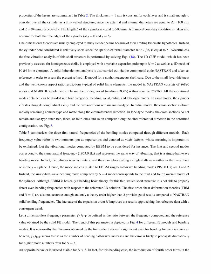
Taking the solid FE model as reference, the results summarized in Table 7 improve again as the expansion order N increases.
In particular, for the present ninth-order model the four-lobe natural frequencies are accurately computed and the agreement
with the 3D solution is remarkable as well as the sizeable reduction in computational cost. On the contrary, the eighth-order
expansion is no longer as refined as was in the analysis of the other vibrational modes. Numerical results are depicted in Fig. 7
in terms of the dimensionless frequency parameter f/ fREF. The trend of the curves is very similar to that illustrated in Fig. 6
corresponding to three-lobe modes. Given a theory, the error decreases as m increases. A remarkable difference between these
figures is that N = 8 is not an appropriate choice to compute the correct four-lobe frequencies.
As far as lobe-type modes are concerned, it is interesting to note a noteworhty behavior that occurs when the half-wave
number m is equal to 1. Sometimes an increment by one of the expansion order N seems to improve the numerical results very
slightly in terms of frequencies computed by CUF models. The particularity stands in the fact that it occurs even when the
convergence on N is not achieved. This particular behavior is clearly shown in Figs. 5−7. For instance, for four-lobe modes
the first frequencies computed by the seventh- and eighth-order models are approximately the same. Regarding three-lobe
modes, the same goes for N = 6 and N = 7. Figure 5 illustrates a similar behavior for the fifth- and sixth-order models.
Looking at the numerical results presented so far, the ninth-order model seems to be refined enough to study the dynamic
behavior of the layered cylinder considered. This statement is confirmed by Table 8, where the first thirty-eight natural
frequencies computed by the present 1D model (N = 9) and the NASTRAN solid model. Each mode presents a superscript
composed of two terms. The first term indicates the kind of mode whereas the second term indicates the value of m. The
results involve bending, radial, axial, two-, three- and four-lobe vibrational modes with an axial half-wave number up to 6.
Despite the one-dimensional approach of the proposed higher-order model, it provides an error lower than 0.8 percent for all
these modes, with a remarkably lower computational effort than that required by the reference solid model. In fact, about a
98% saving of the degrees of freedom involved in the free vibration analysis is obtained. The maximum error is computed for
three- and four-lobe modes, for which an expansion with an even higher order, N = 10 for instance, would further increase the
computational accuracy.
Further results regarding five-lobe modes are not reported here for the sake of brevity. In fact, the same conclusions made

for two-, three- and four-lobe modes would be valid also for more complex lobe-type vibrational modes. However, for the
considered cylinder a ninth-order expansion theory detects vibrational modes with a five-lobe deformation of the cross-section.
Nonetheless, a further increase of N might be required to achieve a good accuracy regarding the numerical frequencies of
these even more complex vibrational modes. This behavior is consistent with the considerations previously mentioned about
the expansion enrichment.
A summary of the first thirty-eight vibrational modes detected by the present one-dimensional models is reported in Table 9,
where the accuracy in computing natural frequencies with respect to the solid FE analysis is shown by varying the expansion
order N. It should be pointed out that a different higher-order expansion is required depending on the kind of vibrational mode
investigated. Some structural models are not even able to detect all the kinds of vibrational modes. For instance, classical
beam theories do not consider radial modes. Third-, fourth- and fifth-order models are necessary to compute two-, three- and
four-lobe modes, respectively. As far as the accuracy is concerned, a further higher expansion order is required. However, the
results show that the introduction of higher-order terms is fundamental for the free vibration analysis of a thin-walled layered
structure, according to previous dynamic response computations through 1D CUF models [38].
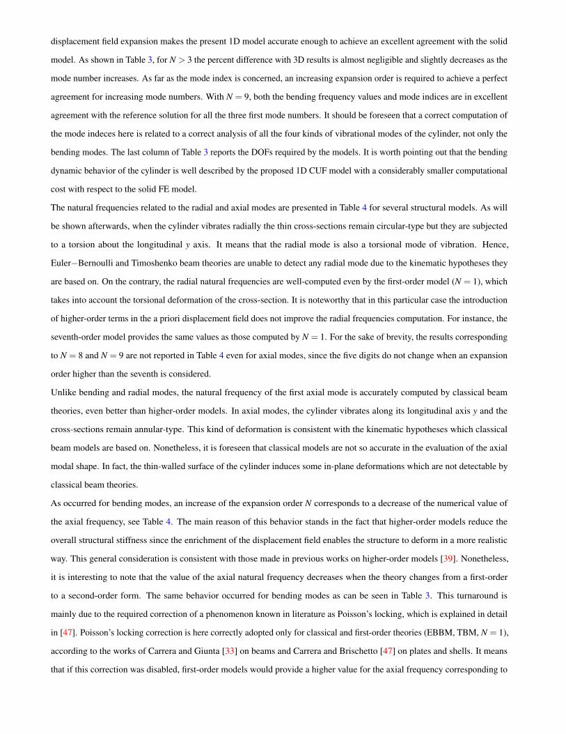
The assessment procedure of 1D CUF models on natural frequencies is now completed. A graphical comparison between the
modal shapes based on the present 1D CUF model and those computed by the solid FEM is now carried out. Some interesting
modal shapes have been chosen and compared in Figs. 8−13. The three-dimensional deformation as well as the front-view of
each modal shape are depicted. It is noteworthy that the modal shapes perfectly match for all the kinds of vibrational modes
considered, including the lobe-type modes which are typical of shell structures.
The lobe-type shapes are correctly described by one-dimensional higher-order models even when these models do not provide
accurate frequencies in comparison with the reference three-dimensional results. For example, the shape of two-lobe modes is
correctly described by using a third-order displacement expansion, although this choice does not provide accurate two-lobe
frequencies in comparison with higher-order models and solid FE solution, see Table 5. As a consequence, when the accuracy
in computing the numerical frequency of a certain lobe-type mode is low, nonetheless the corresponding modal shape is
usually well-described.
Figure 11 highlights the rotation of the cross-sections about the longitudinal y axis that occurs when the cylinder vibrates
radially. Instead, when the cylinder vibrates along its longitudinal y axis, the cross-sections which are close to the clamped
edges are subjected to streching or dilation effects. These effects are emphasized in Fig. 10. Euler−Bernoulli is very effective
in the computation of the axial frequencies of the cylinder, see Table 4. Nonetheless, although the axial mode computed by
Euler−Bernoulli beam theory is not represented here, this classical theory is not able to describe the in-plane deformation of
the compressed and dilated cross-sections. On the contrary, these in-plane deformations are well-described by the present
higher-order 1D models and a good agreement with the three-dimensional solution is achieved not only in the frequency
computation but also in the vibrational shape description, see Fig. 10.
The results in Figs. 8−13 clearly show the accuracy of the present refined model in detecting the three-dimensional deformation
despite its one-dimensional approach, according to previous dynamic computations through 1D CUF models [38]. The present
method shows features not present in standard one-dimensional theories such as the thickness changing of the thin-walled

laminated surface and the in-plane and out-of-plane cross-section deformations. Thus, the proposed modeling approach
appears promising for future additional topics related to shell vibrations and stability. Among these topics, the analysis of
additional geometrical and mechanical boundary conditions, the effect of initial imperfections as well as the extension to
nonlinear problems could be of extreme interest.
5 Conclusions
The free vibration analysis of nonhomogeneous cylindrical shells through refined one-dimensional models is addressed in
this paper. Hierarchical 1D finite elements were formulated on the basis of Carrera Unified Formulation (CUF) and assessed
by comparison with exact solutions of the three-dimensional governing elasticity equations and solid finite element solutions.
As far as the use of higher-order 1D models is concerned, the following main conclusions can be drawn:
1. a different higher-order expansion is required depending on the kind of vibrational mode investigated. Some structural
models are not even able to detect all the kinds of vibrational modes because of the a priori displacement field used. For
instance, none of the lobe-type modes was computed by first- and second-order theories;
2. the introduction of higher-order terms in the displacement field is not always necessary. For example, the first-order
model was accurate enough to provide correct natural frequency values for radial and axial modes;
3. classical beam theories are not able to detect radial and lobe-type vibrational modes, whereas axial frequencies are
correctly computed. Although Euler−Bernoulli’s and Timoshenko’s are basically bending beam theories, for this
thin-walled short structure they are not able to accurately detect even bending natural frequencies;
4. the enrichment of the displacement field enables the structure to deform in a more realistic way and thus leads to capture
vibrational modes that require in-plane and warping deformation to be detected. Higher-order models are required
especially for the evaluation of lobe-type modes, which are typical of shell structures and not detectable by standard
one-dimensional models;
5. in general, an increase of the expansion order corresponds to a decrease of the overall structural stiffness and thus to a
reduction of the frequency values by approaching the three-dimensional results.
As far as the present hierarchical one-dimensional approach is concerned, the results point out that:
a. CUF is the ideal tool to easily compare different higher-order theories. The expansion order of the model, i.e., its accuracy,
is a free parameter of the analysis by exploiting a systematic procedure that leads to governing FE matrices whose form
does not depend on the order of expansion used for the displacement unknowns over the cross-section;
b. despite its one-dimensional approach, the CUF model proved its accuracy in the free vibration analysis of even short,
nonhomogeneous thin- and thick-walled shell structures. Both the modal shapes and natural frequency values are in well
agreement with those obtained by three-dimensional models;
c. a convergent trend of natural frequency values approaching the three-dimensional results as the expansion order increases
is achieved. This proves that the proposed hierarchical model does not introduce additional numerical problems in the
free vibration analysis of layered structures with respect to classical beam theories;

d. the refined 1D CUF model presents a sizeable reduction in computational cost in terms of DOFs with respect to the solid
FE model.
The accurate dynamic study of thin- and thick-walled layered structures can be faced through the present refined 1D approach,
which is a promising numerical tool also for the dynamic response analysis of arbitrary shell structures via a time integration
scheme. The excellent agreement with exact and quasi-exact solutions of the three-dimensional elasticity equations highlights
the shell-type capabilities of the 1D CUF model and the importance of refining the axiomatic displacement field with
higher-order terms.
References
[1] Anderson, J. D., 2010. Fundamentals of Aerodynamics, 5th ed. McGraw-Hill.
[2] Librescu, L., and Na, S., 1998. “Dynamic response of cantilevered thin-walled beams to blast and sonic-boom loadings”.
Shock and Vibration, 5(1), pp. 23–33.
[3] Fung, Y. C., 1993. Biomechanics: Mechanical Properties of Living Tissues, 2nd ed. Springer, New York.
[4] Au, F. T. K., Cheng, Y. S., and Cheung, Y. K., 2001. “Vibration analysis of bridges under moving vehicles and trains: an
overiew”. Progress in Structural Engineering and Materials, 3(3), pp. 299–304.
[5] Qiu, X., Deshpande, V. S., and Fleck, N. A., 2003. “Finite element analysis of the dynamic response of clamped
sandwich beams subject to shock loading”. European Journal of Mechanics A/Solids, 22, pp. 801–814.
[6] Lindeburg, M. R., and McMullin, K. M., 2008. Seismic Design of Building Structures, 9th ed. Professional Publications.
[7] Marur, S. R., and Kant, T., 1997. “On the performance of higher order theories for transient dynamic analysis of
sandwich and composite beams”. Computers & Structures, 65(5), pp. 741–759.
[8] Flugge, W., 1934. Statik und Dynamik der Schalen. Springer-Verlag, Berlin.
[9] Lur’e, A. I., 1940. “The general theory of thin elastic shells”. Prikladnaya Matematika i Mekhanika, 4(2), pp. 7–34.
[10] Byrne, R., 1944. “Theory of small deformations of a thin elastic shell”. University of California, Publications in
Mathematics, 2(1), pp. 103–152.
[11] Love, A. E. H., 2011. A treatise on the mathematical theory of elasticity, 4th ed. Dover Publications.
[12] Sanders, J. L., 1963. “Nonlinear theories for thin shells”. Quarterly of Applied Mathematics, 21(1), pp. 21–36.
[13] Qatu, M. S., 2002. “Recent research advances in the dynamic behavior of shells: 1989–2000, Part 1: Laminated
composite shells”. Applied Mechanics Reviews, 55(4), pp. 325–350.
[14] Qatu, M. S., 2002. “Recent research advances in the dynamic behavior of shells: 1989–2000, Part 2: Homogeneous
shells”. Applied Mechanics Reviews, 55(5), pp. 415–434.
[15] Qatu, M. S., Sullivan, R. W., and Wenchao, W., 2010. “Recent research advances in the dynamic behavior of composite
shells: 2000–2009”. Composite Structures, 93(1), pp. 14–31.
[16] Herrmann, G., and Mirsky, I., 1956. “Three-dimensional and shell-theory analysis of axially symmetric motions of
cylinders”. Journal of Applied Mechanics, 23(4), pp. 563–568.

[17] Mirsky, I., and Herrmann, G., 1957. “Nonaxially symmetric motions of cylindrical shells”. Journal of the Acoustical
Society of America, 29(10), pp. 1116–1123.
[18] Gazis, D. C., 1959. “Three-dimensional investigation of the propagation of waves in hollow circular cylinders. i.
analytical foundation”. Journal of the Acoustical Society of America, 31(5), pp. 568–573.
[19] Armenakas, A. E., Gazis, D. C., and Herrmann, G., 1969. Free vibrations of circular cylindrical shells. Pergamon Press,
Oxford.
[20] Mirsky, I., 1963. “Radial vibrations of thick-walled orthotropic cylinders”. AIAA Journal, 1(2), pp. 487–488.
[21] Soldatos, K. P., 1994. “Review of three dimensional dynamic analyses of circular cylinders and cylindrical shells”.
Applied Mechanics Reviews, 47(10), pp. 501–516.
[22] Soldatos, K. P., and P., H. V., 1990. “Three-dimensional solution of the free vibration problem of homogeneous isotropic
cylindrical shells and panels”. Journal of Sound and Vibration, 137(3), pp. 369–384.
[23] Bhimaraddi, A., 1984. “A higher order theory for free vibration analysis of circular cylindrical shells”. International
Journal of Solids and Structures, 20(7), pp. 623–630.
[24] Timarci, T., and Soldatos, K. P., 2000. “Vibrations of angle-ply laminated circular cylindrical shells subjected to different
sets of edge boundary conditions”. Journal of Engineering Mathematics, 37(1–3), pp. 211–230.
[25] Soldatos, K. P., and Timarci, T., 1993. “A unified formulation of laminated composite, shear deformable, five-degrees-of-
freedom cylindrical shell theories”. Composite Structures, 25(1–4), pp. 165–171.
[26] Mofakhami, M. R., Toudeshky, H. H., and Hashemi, S. H., 2006. “Finite cylinder vibrations with different end boundary
conditions”. Journal of Sound and Vibration, 297(1–2), pp. 293–314.
[27] Alijani, F., and Amabili, M., 2014. “Nonlinear vibrations and multiple resonances of fluid filled arbitrary laminated
circular cylindrical shells”. Composite Structures, 108, pp. 951–962.
[28] Toorani, M. H., and Lakis, A. A., 2006. “Free vibrations of non-uniform composite cylindrical shells”. Nuclear
Engineering and Design, 236(17), pp. 1748–1758.
[29] Khalili, S. M. R., Davar, A., and Malekzadeh Fard, K., 2012. “Free vibration analysis of homogeneous isotropic circular
cylindrical shells based on a new three-dimensional refined higher-order theory”. International Journal of Mechanical
Sciences, 56(1), pp. 1–25.
[30] Bathe, K., 1996. Finite Element Procedures. Prentice Hall, Upper Saddle River, New Jersey.
[31] Euler, L., 1744. De curvis elasticis. Bousquet, Lausanne and Geneva.
[32] Timoshenko, S., 1921. “On the correction for shear of the differential equation for transverse vibrations of prismatic
bars”. Philosophical Magazine, 41, pp. 744–746.
[33] Carrera, E., and Giunta, G., 2010. “Refined beam theories based on a unified formulation”. International Journal of
Applied Mechanics, 2(1), pp. 117–143.
[34] Carrera, E., Giunta, G., and Petrolo, M., 2011. Beam Structures: Classical and Advanced Theories. John Wiley & Sons.
[35] Yu, W., Volovoi, V., Hodges, D., and Hong, X., 2002. “Validation of the variational asymptotic beam sectional analysis
(VABS)”. AIAA Journal, 40(10), pp. 2105–2113.
[36] Silvestre, N., and Camotim, D., 2002. “Second-order generalised beam theory for arbitrary orthotropic materials”.
Thin-Walled Structures, 40(9), pp. 791–820.
[37] Kapania, K., and Raciti, S., 1989. “Recent advances in analysis of laminated beams and plates, Part II: Vibrations and
wave propagation”. AIAA Journal, 27(7), pp. 935–946.
[38] Carrera, E., and Varello, A., 2012. “Dynamic response of thin-walled structures by variable kinematic one-dimensional
models”. Journal of Sound and Vibration, 331(24), pp. 5268–5282.
[39] Carrera, E., Brischetto, S., and Nali, P., 2011. Plates and Shells for Smart Structures: Classical and Advanced Theories
for Modeling and Analysis. John Wiley & Sons.
[40] Carrera, E., Giunta, G., Nali, P., and Petrolo, M., 2010. “Refined beam elements with arbitrary cross-section geometries”.
Computers & Structures, 88(5–6), pp. 283–293.
[41] Carrera, E., and Petrolo, M., 2012. “Refined one-dimensional formulations for laminated structure analysis”. AIAA
Journal, 50(1), pp. 176–189.
[42] Carrera, E., Varello, A., and Demasi, L., 2013. “A refined structural model for static aeroelastic response and divergence
of metallic and composite wings”. CEAS Aeronautical Journal, 4(2), pp. 175–189.
[43] Carrera, E., Petrolo, M., and Varello, A., 2012. “Advanced beam formulations for free vibration analysis of conventional
and joined wings”. Journal of Aerospace Engineering, 25(2), pp. 282–293.
[44] Jones, R., 1999. Mechanics of Composite Materials, 2nd ed. Taylor & Francis, Philadelphia.
[45] Almroth, B. O., 1966. “Influence of edge conditions on the stability of axially compressed cylindrical shells”. AIAA
Journal, 4(1), pp. 134–140.
[46] Carrera, E., Zappino, E., and Petrolo, M., 2012. “Analysis of thin-walled structures with longitudinal and transversal
stiffeners”. Journal of Applied Mechanics. In press, DOI:10.1115/1.4006939.
[47] Carrera, E., and Brischetto, S., 2008. “Analysis of thickness locking in classical, refined and mixed multilayered plate
theories”. Composite Structures, 82(4), pp. 549–562.
[48] Carrera, E., Petrolo, M., and Nali, P., 2010. “Unified formulation applied to free vibrations finite element analysis of
beams with arbitrary section”. Shock and Vibrations, 18, pp. 485–502.

Table captions
Table 1:
Comparison of frequency parameters ω based on the present 1D models with 3D elasticity solutions. m = 1.
Table 2:
Material and geometrical properties of the cylinder layers.
Table 3:
Comparison of natural frequencies [Hz] based on the present 1D models with 3D FE solution. Bending modes.
Table 4:
Comparison of natural frequencies [Hz] based on the present 1D models with 3D FE solution. Radial and axial modes.
Table 5:
Comparison of natural frequencies [Hz] based on the present 1D models with 3D FE solution. Two-lobe modes.
Table 6:
Comparison of natural frequencies [Hz] based on the present 1D models with 3D FE solution. Three-lobe modes.
Table 7:
Comparison of natural frequencies [Hz] based on the present 1D models with 3D FE solution. Four-lobe modes.
Table 8:
Natural frequencies [Hz] of the first thirty-eight vibrational modes of the cylinder.
Table 9:
Summary of the vibrational modes detected with an increasing expansion order N by 1D models and comparison of the
corresponding natural frequencies with 3D FE solution.

Figure captions
Figure 1:
Cross-sections geometry for the one-layer and three-layer cylinders.
Figure 1a:
One-layer cylinder
Figure 1b:
Three-layer cylinder
Figure 2:
Procedure to build the element structural stiffness matrix KEL of a B3 element with N = 2.
Figure 3:
Cross-section deformation for different lobe-type modes.
Figure 4:
Dimensionless frequency parameter for different 1D models. Bending modes.
Figure 5:
Dimensionless frequency parameter for different 1D models. Two-lobe modes.
Figure 6:
Dimensionless frequency parameter for different 1D models. Three-lobe modes.
Figure 7:
Dimensionless frequency parameter for different 1D models. Four-lobe modes.
Figure 8:
Third bending modal shape (b.3).
Figure 8a:
Present 1D model
Figure 8b:
NASTRAN solid model
Figure 9:
Second radial modal shape (r.2).

Figure 9a:
Present 1D model
Figure 9b:
NASTRAN solid model
Figure 10:
First axial modal shape (a.1).
Figure 10a:
Present 1D model
Figure 10b:
NASTRAN solid model
Figure 11:
Fifth two-lobe modal shape (2.5).
Figure 11a:
Present 1D model
Figure 11b:
NASTRAN solid model
Figure 12:
Fourth three-lobe modal shape (3.4).
Figure 12a:
Present 1D model
Figure 12b:
NASTRAN solid model
Figure 13:
Second four-lobe modal shape (4.2).
Figure 13a:
Present 1D model
Figure 13b:
NASTRAN solid model

Tables
Table 1. Comparison of frequency parameters ω based on the present 1D models with 3D elasticity solutions. m = 1.
t/R n N = 4 N = 7 N = 9 Exact 3D [19] 3D [22]
0.1 2 I 1.0804 1.0620 1.0620 1.0623 1.0624
II 2.3758 2.3745 2.3744 2.3744 2.3745
III 3.9659 3.9634 3.9632 3.9634 3.9634
4 I 0.9937 0.8838 0.8819 0.8823 0.8826
II 2.9118 2.7160 2.7159 2.7159 2.7159
III 4.8497 4.4877 4.4875 4.4874 4.4876
6 I 1.7500 0.8388 0.8112 0.8093 0.8096
II 4.1441 3.1562 3.1534 3.1533 3.1533
III 5.9431 5.2485 5.2367 5.2365 5.2367
0.2 2 I 1.2430 1.1891 1.1887 1.1889 1.1891
II 2.3806 2.3757 2.3757 2.3757 2.3758
III 3.9620 3.9531 3.9529 3.9527 3.9528
4 I 1.2823 1.1184 1.1015 1.1009 1.1012
II 2.9260 2.7192 2.7182 2.7182 2.7184
III 4.7903 4.4667 4.4661 4.4659 4.4661
6 I 1.8907 1.2647 1.2181 1.1975 1.1979
II 4.0979 3.1688 3.1569 3.1566 3.1569
III 5.8511 5.2247 5.1965 5.1949 5.1952
Table 2. Material and geometrical properties of the cylinder layers.
Property Layer 1 Layer 2 Layer 3
t [mm] 1 1 1
E [GPa] 69 30 15
ν 0.33 0.33 0.33
ρ [kg/m3] 2700 2000 1800

Table 3. Comparison of natural frequencies [Hz] based on the present 1D models with 3D FE solution. Bending modes.
ModelMode number
1 2 3DOFs
EBBM 1963.0 1,2 5044.9 4,5 9014.9 7,8 93
TBM 1572.6 1,2 3530.3 3,4 5823.0 6,7 155
N = 1 1572.6 1,2 3530.3 6,7 5823.0 12,13 279
N = 2 1597.7 1,2 3562.1 4,5 5852.6 8,9 558
N = 3 1368.0 1,2 2925.0 6,7 4725.5 11,12 930
N = 4 1365.4 3,4 2912.6 10,11 4679.5 19,20 1395
N = 5 1364.3 3,4 2909.7 10,11 4674.0 25,26 1953
N = 6 1364.3 3,4 2909.6 16,17 4673.9 25,26 2604
N = 7 1364.2 3,4 2909.5 16,17 4673.8 29,30 3348
N = 8 1364.2 3,4 2909.5 16,17 4673.8 33,34 4185
N = 9 1364.0 3,4 2908.6 16,17 4671.0 37,38 5115
Solid FEM 1360.9 3,4 2906.3 16,17 4670.9 37,38 257760
Table 4. Comparison of natural frequencies [Hz] based on the present 1D models with 3D FE solution. Radial and axial modes.
ModelRadial Axial
Mode 1 Mode 2 Mode 1DOFs
EBBM − − 4173.2 3 93
TBM − − 4173.2 5 155
N = 1 2540.9 4 5081.7 10 4173.3 8 279
N = 2 2540.9 3 5081.7 7 4191.3 6 558
N = 3 2540.9 5 5081.7 15 4182.5 10 930
N = 4 2540.9 7 5081.7 23 4182.4 18 1395
N = 5 2540.9 7 5081.7 29 4182.1 22 1953
N = 6 2540.9 11 5081.7 31 4182.0 24 2604
N = 7 2540.9 11 5081.7 39 4182.0 24 3348
Solid FEM 2540.2 13 5080.1 43 4172.2 32 257760

Table 5. Comparison of natural frequencies [Hz] based on the present 1D models with 3D FE solution. Two-lobe modes.
ModelMode number
1 2 3 4 5
N = 3 1617.9 3,4 2960.7 8,9 4755.5 13,14 6832.6 18,19 9094.5 24,25
N = 4 1209.1 1,2 1795.0 5,6 2732.8 8,9 3850.7 14,15 5049.5 21,22
N = 5 1005.4 1,2 1666.3 5,6 2643.3 8,9 3765.4 18,19 4937.7 27,28
N = 6 995.8 1,2 1640.9 5,6 2602.6 12,13 3707.4 20,21 4859.5 27,28
N = 7 862.7 1,2 1561.9 5,6 2551.7 12,13 3670.0 20,21 4829.1 35,36
N = 8 862.6 1,2 1561.6 5,6 2551.3 14,15 3669.4 20,21 4828.0 35,36
N = 9 860.4 1,2 1560.3 5,6 2550.6 14,15 3669.3 24,25 4827.4 39,40
Solid FEM 859.9 1,2 1557.0 5,6 2545.4 14,15 3662.9 24,25 4820.9 41,42
Table 6. Comparison of natural frequencies [Hz] based on the present 1D models with 3D FE solution. Three-lobe modes.
ModelMode number
1 2 3 4 5 6
N = 4 3281.2 12,13 4099.2 16,17 5354.2 24,25 6946.7 30,31 8795.1 40,41 10837.6 53,54
N = 5 3027.4 12,13 3160.3 14,15 3453.3 16,17 3930.7 20,21 4572.9 23,24 5339.8 30,31
N = 6 2319.2 7,8 2504.7 9,10 2882.6 14,15 3454.6 18,19 4178.1 22,23 5001.9 29,30
N = 7 2306.9 7,8 2458.7 9,10 2789.4 14,15 3308.7 18,19 3978.0 22,23 4746.3 33,34
N = 8 1826.3 7,8 2006.7 9,10 2390.3 11,12 2968.6 18,19 3688.1 22,23 4493.8 29,30
N = 9 1826.2 7,8 2006.2 9,10 2389.1 11,12 2966.7 18,19 3685.0 26,27 4490.2 35,36
Solid FEM 1818.0 7,8 1997.1 9,10 2378.6 11,12 2954.9 18,19 3672.2 26,27 4475.1 35,36
Table 7. Comparison of natural frequencies [Hz] based on the present 1D models with 3D FE solution. Four-lobe modes.
ModelMode number
1 2 3 4 5 6
N = 5 5961.4 32,33 6489.5 40,41 7350.1 46,47 8512.2 56,57 9937.2 66,67 11585.3 86,87
N = 6 5805.4 32,33 5877.9 34,35 6017.7 40,41 6243.3 42,43 6527.3 46,47 6993.4 50,51
N = 7 4380.8 25,26 4494.4 27,28 4702.8 31,32 5020.9 37,38 5453.5 40,41 5994.1 46,47
N = 8 4368.4 25,26 4445.6 27,28 4595.8 31,32 4837.5 37,38 5180.6 40,41 5623.1 44,45
N = 9 3441.1 20,21 3528.8 22,23 3700.4 28,29 3976.8 30,31 4364.8 33,34 4856.7 41,42
Solid FEM 3417.8 20,21 3503.3 22,23 3672.4 28,29 3945.3 30,31 4329.1 33,34 4816.1 39,40

Table 8. Natural frequencies [Hz] of the first thirty-eight vibrational modes of the cylinder.
Mode N = 9 Solid FEM % Difference
1 , 2 2.1 860.4 859.9 0.058
3 , 4 b.1 1364.0 1360.9 0.228
5 , 6 2.2 1560.3 1557.0 0.212
7 , 8 3.1 1826.2 1818.0 0.451
9 , 10 3.2 2006.2 1997.1 0.456
11 , 12 3.3 2389.1 2378.6 0.441
13 r.1 2540.9 2540.2 0.028
14 , 15 2.3 2550.6 2545.4 0.204
16 , 17 b.2 2908.6 2906.3 0.079
18 , 19 3.4 2966.7 2954.9 0.399
20 , 21 4.1 3441.1 3417.8 0.682
22 , 23 4.2 3528.8 3503.3 0.728
24 , 25 2.4 3669.3 3662.9 0.175
26 , 27 3.5 3685.0 3672.2 0.349
28 , 29 4.3 3700.4 3672.4 0.762
30 , 31 4.4 3976.8 3945.3 0.798
32 a.1 4190.6 4172.2 0.441
33 , 34 4.5 4364.8 4329.1 0.825
35 , 36 3.6 4490.2 4475.1 0.337
37 , 38 b.3 4671.0 4670.9 0.002
DOFs 5115 257760 −98.02
2.1: two-lobe mode, m = 1 b.1: bending mode, m = 1
3.1: three-lobe mode, m = 1 r.1: radial mode, m = 1
4.1: four-lobe mode, m = 1 a.1: axial mode, m = 1
4.5: four-lobe mode, m = 5

Table 9. Summary of the vibrational modes detected with an increasing expansion order N by 1D models and comparison of the corre-sponding natural frequencies with 3D FE solution.
ModelVibrational mode
2.1 b.1 2.2 3.1 3.2 3.3 r.1 2.3 b.2 3.4 4.1 4.2 2.4 3.5 4.3 4.4 a.1 4.5 3.6 b.3
EBBM 6 6 f 6
TBM 6 f 6
N = 1 f 6 f 6
N = 2 f 6 f 6
N = 3 6 f 6 f 6 f 6 f ?
N = 4 6 f 6 6 6 f ? f 6 ? 6 f 6 f
N = 5 f ? 6 6 6 f ? f 6 6 6 ? 6 6 6 f 6 f
N = 6 f ? 6 6 6 f ? f 6 6 ? 6 6 f 6 f
N = 7 f f f 6 6 f f f 6 6 f ? 6 6 f 6 ? f
N = 8 f f f f f f f f f f 6 6 f f 6 6 f f f
N = 9 f f f f f f f f f f f f f f f f f f f f
Mode not detected. ? Mode detected. 1%≤ Error < 10%.
6 Mode detected. Error > 20%. f Mode detected. Error < 1%.
Mode detected. 10%≤ Error ≤ 20%.

Figures
t
x
z
y
R
(a) One-layer cylinder
di
x
z
321
y
de
(b) Three-layer cylinder
Fig. 1. Cross-sections geometry for the one-layer and three-layer cylinders.

Kijxx
Kyx
Kzx Kzy Kzz
KyzKyy
Kxy Kxzx
y
z
x y z
=1
=2
=3
=4
=5
=6
=1s =2s =3s =4s =5s =6s
s
s
Node 1
j
i
Node 3
Node 2
Node 1
EL
EL
EL
ELNode 3 Node 2
EL
KEL
EL
s ij s ij s
ij s ij s ij s
ij s ij s ij s
Fig. 2. Procedure to build the element structural stiffness matrix KEL of a B3 element with N = 2.

Undeformed
Two-lobe
Three-lobe
Four-lobe
Fig. 3. Cross-section deformation for different lobe-type modes.
0.9
1
1.1
1.2
1.3
1.4
1.5
1.61.71.81.9
2
1 2 3
f / f R
EF
Mode number
EBBMN = 1
N = 3N = 4
N = 5Solid FEM
Fig. 4. Dimensionless frequency parameter for different 1D models. Bending modes.

0.95
1
1.05
1.1
1.15
1.2
1.25
1.3
1.35
1.4
1.45
1 2 3 4 5
f / f R
EF
Mode number
N = 4N = 5
N = 6N = 7
N = 8N = 9
Solid FEM
Fig. 5. Dimensionless frequency parameter for different 1D models. Two-lobe modes.
0.9
1
1.1
1.2
1.3
1.4
1.5
1.6
1.7
1 2 3 4 5 6
f / f R
EF
Mode number
N = 5N = 6
N = 7N = 8
N = 9Solid FEM
Fig. 6. Dimensionless frequency parameter for different 1D models. Three-lobe modes.
0.9
1
1.1
1.2
1.3
1.4
1.5
1.6
1.7
1 2 3 4 5
f / f R
EF
Mode number
N = 6N = 7
N = 8N = 9
Solid FEM
Fig. 7. Dimensionless frequency parameter for different 1D models. Four-lobe modes.
(a) Present 1D model (b) NASTRAN solid model
Fig. 8. Third bending modal shape (b.3).
(a) Present 1D model (b) NASTRAN solid model
Fig. 9. Second radial modal shape (r.2).
(a) Present 1D model (b) NASTRAN solid model
Fig. 10. First axial modal shape (a.1).

(a) Present 1D model (b) NASTRAN solid model
Fig. 11. Fifth two-lobe modal shape (2.5).
(a) Present 1D model (b) NASTRAN solid model
Fig. 12. Fourth three-lobe modal shape (3.4).
(a) Present 1D model (b) NASTRAN solid model
Fig. 13. Second four-lobe modal shape (4.2).