fracture mechanics lecture notes - civil, environmental, and

Draft

Lecture Notes in:

FRACTURE MECHANICS

Victor E. SaoumaDept. of Civil Environmental and Architectural Engineering

University of Colorado, Boulder, CO 80309-0428

Draft

Contents

1 INTRODUCTION 11.1 Modes of Failures . . . . . . . . . . . . . . . . . . . . . . . . . . . . . . . . . . . . 11.2 Examples of Structural Failures Caused by Fracture . . . . . . . . . . . . . . . . 21.3 Fracture Mechanics vs Strength of Materials . . . . . . . . . . . . . . . . . . . . . 31.4 Major Historical Developments in Fracture Mechanics . . . . . . . . . . . . . . . 61.5 Coverage . . . . . . . . . . . . . . . . . . . . . . . . . . . . . . . . . . . . . . . . . 8

2 PRELIMINARY CONSIDERATIONS 12.1 Tensors . . . . . . . . . . . . . . . . . . . . . . . . . . . . . . . . . . . . . . . . . 1

2.1.1 Indicial Notation . . . . . . . . . . . . . . . . . . . . . . . . . . . . . . . . 22.1.2 Tensor Operations . . . . . . . . . . . . . . . . . . . . . . . . . . . . . . . 32.1.3 Rotation of Axes . . . . . . . . . . . . . . . . . . . . . . . . . . . . . . . . 52.1.4 Trace . . . . . . . . . . . . . . . . . . . . . . . . . . . . . . . . . . . . . . 52.1.5 Inverse Tensor . . . . . . . . . . . . . . . . . . . . . . . . . . . . . . . . . 62.1.6 Principal Values and Directions of Symmetric Second Order Tensors . . . 6

2.2 Kinetics . . . . . . . . . . . . . . . . . . . . . . . . . . . . . . . . . . . . . . . . . 72.2.1 Force, Traction and Stress Vectors . . . . . . . . . . . . . . . . . . . . . . 72.2.2 Traction on an Arbitrary Plane; Cauchy’s Stress Tensor . . . . . . . . . . 8E 2-1 Stress Vectors . . . . . . . . . . . . . . . . . . . . . . . . . . . . . . . . . . 92.2.3 Invariants . . . . . . . . . . . . . . . . . . . . . . . . . . . . . . . . . . . . 102.2.4 Spherical and Deviatoric Stress Tensors . . . . . . . . . . . . . . . . . . . 102.2.5 Stress Transformation . . . . . . . . . . . . . . . . . . . . . . . . . . . . . 112.2.6 Polar Coordinates . . . . . . . . . . . . . . . . . . . . . . . . . . . . . . . 11

2.3 Kinematic . . . . . . . . . . . . . . . . . . . . . . . . . . . . . . . . . . . . . . . . 112.3.1 Strain Tensors . . . . . . . . . . . . . . . . . . . . . . . . . . . . . . . . . 112.3.2 Compatibility Equation . . . . . . . . . . . . . . . . . . . . . . . . . . . . 13

2.4 Fundamental Laws of Continuum Mechanics . . . . . . . . . . . . . . . . . . . . . 142.4.1 Conservation Laws . . . . . . . . . . . . . . . . . . . . . . . . . . . . . . . 142.4.2 Fluxes . . . . . . . . . . . . . . . . . . . . . . . . . . . . . . . . . . . . . . 152.4.3 Conservation of Mass; Continuity Equation . . . . . . . . . . . . . . . . . 162.4.4 Linear Momentum Principle; Equation of Motion . . . . . . . . . . . . . . 162.4.5 Moment of Momentum Principle . . . . . . . . . . . . . . . . . . . . . . . 172.4.6 Conservation of Energy; First Principle of Thermodynamics . . . . . . . . 18

2.5 Constitutive Equations . . . . . . . . . . . . . . . . . . . . . . . . . . . . . . . . . 182.5.1 Transversly Isotropic Case . . . . . . . . . . . . . . . . . . . . . . . . . . . 202.5.2 Special 2D Cases . . . . . . . . . . . . . . . . . . . . . . . . . . . . . . . . 20

2.5.2.1 Plane Strain . . . . . . . . . . . . . . . . . . . . . . . . . . . . . 20

DraftCONTENTS iii

5.1.1.2 Ideal Strength in Terms of Engineering Parameter . . . . . . . . 45.1.2 Shear Strength . . . . . . . . . . . . . . . . . . . . . . . . . . . . . . . . . 5

5.2 Griffith Theory . . . . . . . . . . . . . . . . . . . . . . . . . . . . . . . . . . . . . 55.2.1 Derivation . . . . . . . . . . . . . . . . . . . . . . . . . . . . . . . . . . . . 6

6 ENERGY TRANSFER in CRACK GROWTH; (Griffith II) 16.1 Thermodynamics of Crack Growth . . . . . . . . . . . . . . . . . . . . . . . . . . 1

6.1.1 General Derivation . . . . . . . . . . . . . . . . . . . . . . . . . . . . . . . 16.1.2 Brittle Material, Griffith’s Model . . . . . . . . . . . . . . . . . . . . . . . 2

6.2 Energy Release Rate; Global . . . . . . . . . . . . . . . . . . . . . . . . . . . . . 56.2.1 From Load-Displacement . . . . . . . . . . . . . . . . . . . . . . . . . . . 56.2.2 From Compliance . . . . . . . . . . . . . . . . . . . . . . . . . . . . . . . . 6

6.3 Energy Release Rate; Local . . . . . . . . . . . . . . . . . . . . . . . . . . . . . . 86.4 Crack Stability . . . . . . . . . . . . . . . . . . . . . . . . . . . . . . . . . . . . . 10

6.4.1 Effect of Geometry; Π Curve . . . . . . . . . . . . . . . . . . . . . . . . . 106.4.2 Effect of Material; R Curve . . . . . . . . . . . . . . . . . . . . . . . . . . 12

6.4.2.1 Theoretical Basis . . . . . . . . . . . . . . . . . . . . . . . . . . . 126.4.2.2 R vs KIc . . . . . . . . . . . . . . . . . . . . . . . . . . . . . . . 126.4.2.3 Plane Strain . . . . . . . . . . . . . . . . . . . . . . . . . . . . . 136.4.2.4 Plane Stress . . . . . . . . . . . . . . . . . . . . . . . . . . . . . 14

7 MIXED MODE CRACK PROPAGATION 17.1 Analytical Models for Isotropic Solids . . . . . . . . . . . . . . . . . . . . . . . . 2

7.1.1 Maximum Circumferential Tensile Stress. . . . . . . . . . . . . . . . . . . 27.1.2 Maximum Energy Release Rate . . . . . . . . . . . . . . . . . . . . . . . . 37.1.3 Minimum Strain Energy Density Criteria. . . . . . . . . . . . . . . . . . . 47.1.4 Observations . . . . . . . . . . . . . . . . . . . . . . . . . . . . . . . . . . 6

7.2 Empirical Models for Rocks . . . . . . . . . . . . . . . . . . . . . . . . . . . . . . 87.3 Extensions to Anisotropic Solids . . . . . . . . . . . . . . . . . . . . . . . . . . . 97.4 Interface Cracks . . . . . . . . . . . . . . . . . . . . . . . . . . . . . . . . . . . . 13

7.4.1 Crack Tip Fields . . . . . . . . . . . . . . . . . . . . . . . . . . . . . . . . 157.4.2 Dimensions of Bimaterial Stress Intensity Factors . . . . . . . . . . . . . . 167.4.3 Interface Fracture Toughness . . . . . . . . . . . . . . . . . . . . . . . . . 17

7.4.3.1 Interface Fracture Toughness when β = 0 . . . . . . . . . . . . . 197.4.3.2 Interface Fracture Toughness when β 6= 0 . . . . . . . . . . . . . 20

7.4.4 Crack Kinking Analysis . . . . . . . . . . . . . . . . . . . . . . . . . . . . 207.4.4.1 Numerical Results from He and Hutchinson . . . . . . . . . . . 217.4.4.2 Numerical Results Using Merlin . . . . . . . . . . . . . . . . . . 22

7.4.5 Summary . . . . . . . . . . . . . . . . . . . . . . . . . . . . . . . . . . . . 25

II ELASTO PLASTIC FRACTURE MECHANICS 29

8 PLASTIC ZONE SIZES 18.1 Uniaxial Stress Criteria . . . . . . . . . . . . . . . . . . . . . . . . . . . . . . . . 1

8.1.1 First-Order Approximation. . . . . . . . . . . . . . . . . . . . . . . . . . . 28.1.2 Second-Order Approximation (Irwin) . . . . . . . . . . . . . . . . . . . . . 2

8.1.2.1 Example . . . . . . . . . . . . . . . . . . . . . . . . . . . . . . . 4

Victor Saouma Fracture Mechanics

DraftCONTENTS v

11.11Dynamic Energy Release Rate . . . . . . . . . . . . . . . . . . . . . . . . . . . . 3111.12Effect of Other Loading . . . . . . . . . . . . . . . . . . . . . . . . . . . . . . . . 33

11.12.1Surface Tractions on Crack Surfaces . . . . . . . . . . . . . . . . . . . . . 3311.12.2Body Forces . . . . . . . . . . . . . . . . . . . . . . . . . . . . . . . . . . . 3311.12.3 Initial Strains Corresponding to Thermal Loading . . . . . . . . . . . . . 3411.12.4 Initial Stresses Corresponding to Pore Pressures . . . . . . . . . . . . . . 3511.12.5Combined Thermal Strains and Pore Pressures . . . . . . . . . . . . . . . 37

11.13Epilogue . . . . . . . . . . . . . . . . . . . . . . . . . . . . . . . . . . . . . . . . . 38

IV FRACTURE MECHANICS OF CONCRETE 41

12 FRACTURE DETERIORATION ANALYSIS OF CONCRETE 112.1 Introduction . . . . . . . . . . . . . . . . . . . . . . . . . . . . . . . . . . . . . . . 112.2 Phenomenological Observations . . . . . . . . . . . . . . . . . . . . . . . . . . . . 2

12.2.1 Load, Displacement, and Strain Control Tests . . . . . . . . . . . . . . . . 212.2.2 Pre/Post-Peak Material Response of Steel and Concrete . . . . . . . . . . 3

12.3 Localisation of Deformation . . . . . . . . . . . . . . . . . . . . . . . . . . . . . . 412.3.1 Experimental Evidence . . . . . . . . . . . . . . . . . . . . . . . . . . . . 4

12.3.1.1 σ-COD Diagram, Hillerborg’s Model . . . . . . . . . . . . . . . . 512.3.2 Theoretical Evidence . . . . . . . . . . . . . . . . . . . . . . . . . . . . . . 7

12.3.2.1 Static Loading . . . . . . . . . . . . . . . . . . . . . . . . . . . . 712.3.2.2 Dynamic Loading . . . . . . . . . . . . . . . . . . . . . . . . . . 11

12.3.2.2.1 Loss of Hyperbolicity . . . . . . . . . . . . . . . . . . . 1112.3.2.2.2 Wave Equation for Softening Maerials . . . . . . . . . . 11

12.3.3 Conclusion . . . . . . . . . . . . . . . . . . . . . . . . . . . . . . . . . . . 1312.4 Griffith Criterion and FPZ . . . . . . . . . . . . . . . . . . . . . . . . . . . . . . . 13

13 FRACTURE MECHANICS of CONCRETE 113.1 Linear Elastic Fracture Models . . . . . . . . . . . . . . . . . . . . . . . . . . . . 1

13.1.1 Finite Element Calibration . . . . . . . . . . . . . . . . . . . . . . . . . . 213.1.2 Testing Procedure . . . . . . . . . . . . . . . . . . . . . . . . . . . . . . . 313.1.3 Data Reduction . . . . . . . . . . . . . . . . . . . . . . . . . . . . . . . . . 3

13.2 Nonlinear Fracture Models . . . . . . . . . . . . . . . . . . . . . . . . . . . . . . . 513.2.1 Hillerborg Characteristic Length . . . . . . . . . . . . . . . . . . . . . . . 5

13.2.1.1 MIHASHI data . . . . . . . . . . . . . . . . . . . . . . . . . . . . 613.2.2 Jenq and Shah Two Parameters Model . . . . . . . . . . . . . . . . . . . . 613.2.3 Size Effect Law, Bazant . . . . . . . . . . . . . . . . . . . . . . . . . . . . 713.2.4 Carpinteri Brittleness Number . . . . . . . . . . . . . . . . . . . . . . . . 7

13.3 Comparison of the Fracture Models . . . . . . . . . . . . . . . . . . . . . . . . . . 813.3.1 Hillerborg Characteristic Length, lch . . . . . . . . . . . . . . . . . . . . . 813.3.2 Bazant Brittleness Number, β . . . . . . . . . . . . . . . . . . . . . . . . . 913.3.3 Carpinteri Brittleness Number, s . . . . . . . . . . . . . . . . . . . . . . . 913.3.4 Jenq and Shah’s Critical Material Length, Q . . . . . . . . . . . . . . . . 1013.3.5 Discussion . . . . . . . . . . . . . . . . . . . . . . . . . . . . . . . . . . . . 10

13.4 Model Selection . . . . . . . . . . . . . . . . . . . . . . . . . . . . . . . . . . . . . 10


DraftCONTENTS vii

V FINITE ELEMENT TECHNIQUES IN FRACTURE MECHANICS 15

17 SINGULAR ELEMENT 117.1 Introduction . . . . . . . . . . . . . . . . . . . . . . . . . . . . . . . . . . . . . . . 117.2 Displacement Extrapolation . . . . . . . . . . . . . . . . . . . . . . . . . . . . . . 117.3 Quarter Point Singular Elements . . . . . . . . . . . . . . . . . . . . . . . . . . . 217.4 Review of Isoparametric Finite Elements . . . . . . . . . . . . . . . . . . . . . . . 317.5 How to Distort the Element to Model the Singularity . . . . . . . . . . . . . . . . 517.6 Order of Singularity . . . . . . . . . . . . . . . . . . . . . . . . . . . . . . . . . . 617.7 Stress Intensity Factors Extraction . . . . . . . . . . . . . . . . . . . . . . . . . . 7

17.7.1 Isotropic Case . . . . . . . . . . . . . . . . . . . . . . . . . . . . . . . . . . 817.7.2 Anisotropic Case . . . . . . . . . . . . . . . . . . . . . . . . . . . . . . . . 9

17.8 Numerical Evaluation . . . . . . . . . . . . . . . . . . . . . . . . . . . . . . . . . 917.9 Historical Overview . . . . . . . . . . . . . . . . . . . . . . . . . . . . . . . . . . . 1017.10Other Singular Elements . . . . . . . . . . . . . . . . . . . . . . . . . . . . . . . . 12

18 ENERGY RELEASE BASED METHODS 118.1 Mode I Only . . . . . . . . . . . . . . . . . . . . . . . . . . . . . . . . . . . . . . 1

18.1.1 Energy Release Rate . . . . . . . . . . . . . . . . . . . . . . . . . . . . . . 118.1.2 Virtual Crack Extension. . . . . . . . . . . . . . . . . . . . . . . . . . . . 2

18.2 Mixed Mode Cases . . . . . . . . . . . . . . . . . . . . . . . . . . . . . . . . . . . 318.2.1 Two Virtual Crack Extensions. . . . . . . . . . . . . . . . . . . . . . . . . 318.2.2 Single Virtual Crack Extension, Displacement Decomposition . . . . . . . 4

19 J INTEGRAL BASED METHODS 119.1 Numerical Evaluation . . . . . . . . . . . . . . . . . . . . . . . . . . . . . . . . . 119.2 Mixed Mode SIF Evaluation . . . . . . . . . . . . . . . . . . . . . . . . . . . . . . 419.3 Equivalent Domain Integral (EDI) Method . . . . . . . . . . . . . . . . . . . . . 5

19.3.1 Energy Release Rate J . . . . . . . . . . . . . . . . . . . . . . . . . . . . . 619.3.1.1 2D case . . . . . . . . . . . . . . . . . . . . . . . . . . . . . . . . 619.3.1.2 3D Generalization . . . . . . . . . . . . . . . . . . . . . . . . . . 8

19.3.2 Extraction of SIF . . . . . . . . . . . . . . . . . . . . . . . . . . . . . . . . 1019.3.2.1 J Components . . . . . . . . . . . . . . . . . . . . . . . . . . . . 1119.3.2.2 σ and u Decomposition . . . . . . . . . . . . . . . . . . . . . . . 11

20 RECIPROCAL WORK INTEGRALS 120.1 General Formulation . . . . . . . . . . . . . . . . . . . . . . . . . . . . . . . . . . 120.2 Volume Form of the Reciprocal Work Integral . . . . . . . . . . . . . . . . . . . . 520.3 Surface Tractions on Crack Surfaces . . . . . . . . . . . . . . . . . . . . . . . . . 720.4 Body Forces . . . . . . . . . . . . . . . . . . . . . . . . . . . . . . . . . . . . . . . 820.5 Initial Strains Corresponding to Thermal Loading . . . . . . . . . . . . . . . . . 820.6 Initial Stresses Corresponding to Pore Pressures . . . . . . . . . . . . . . . . . . . 1020.7 Combined Thermal Strains and Pore Pressures . . . . . . . . . . . . . . . . . . . 1120.8 Field Equations for Thermo- and Poro-Elasticity . . . . . . . . . . . . . . . . . . 11


Draft

List of Figures

1.1 Cracked Cantilevered Beam . . . . . . . . . . . . . . . . . . . . . . . . . . . . . . 31.2 Failure Envelope for a Cracked Cantilevered Beam . . . . . . . . . . . . . . . . . 41.3 Generalized Failure Envelope . . . . . . . . . . . . . . . . . . . . . . . . . . . . . 51.4 Column Curve . . . . . . . . . . . . . . . . . . . . . . . . . . . . . . . . . . . . . 5

2.1 Stress Components on an Infinitesimal Element . . . . . . . . . . . . . . . . . . . 72.2 Stresses as Tensor Components . . . . . . . . . . . . . . . . . . . . . . . . . . . . 82.3 Cauchy’s Tetrahedron . . . . . . . . . . . . . . . . . . . . . . . . . . . . . . . . . 92.4 Flux Through Area dS . . . . . . . . . . . . . . . . . . . . . . . . . . . . . . . . . 152.5 Equilibrium of Stresses, Cartesian Coordinates . . . . . . . . . . . . . . . . . . . 172.6 Curvilinear Coordinates . . . . . . . . . . . . . . . . . . . . . . . . . . . . . . . . 252.7 Transversly Isotropic Material . . . . . . . . . . . . . . . . . . . . . . . . . . . . . 262.8 Coordinate Systems for Stress Transformations . . . . . . . . . . . . . . . . . . . 28

3.1 Circular Hole in an Infinite Plate . . . . . . . . . . . . . . . . . . . . . . . . . . . 23.2 Elliptical Hole in an Infinite Plate . . . . . . . . . . . . . . . . . . . . . . . . . . 53.3 Crack in an Infinite Plate . . . . . . . . . . . . . . . . . . . . . . . . . . . . . . . 73.4 Independent Modes of Crack Displacements . . . . . . . . . . . . . . . . . . . . . 113.5 Plate with Angular Corners . . . . . . . . . . . . . . . . . . . . . . . . . . . . . . 143.6 Plate with Angular Corners . . . . . . . . . . . . . . . . . . . . . . . . . . . . . . 18

4.1 Middle Tension Panel . . . . . . . . . . . . . . . . . . . . . . . . . . . . . . . . . 24.2 Single Edge Notch Tension Panel . . . . . . . . . . . . . . . . . . . . . . . . . . . 34.3 Double Edge Notch Tension Panel . . . . . . . . . . . . . . . . . . . . . . . . . . 34.4 Three Point Bend Beam . . . . . . . . . . . . . . . . . . . . . . . . . . . . . . . . 44.5 Compact Tension Specimen . . . . . . . . . . . . . . . . . . . . . . . . . . . . . . 44.6 Approximate Solutions for Two Opposite Short Cracks Radiating from a Circular Hole in an Infinite Plate under Tension 54.7 Approximate Solutions for Long Cracks Radiating from a Circular Hole in an Infinite Plate under Tension 64.8 Radiating Cracks from a Circular Hole in an Infinite Plate under Biaxial Stress . 64.9 Pressurized Hole with Radiating Cracks . . . . . . . . . . . . . . . . . . . . . . . 74.10 Two Opposite Point Loads acting on the Surface of an Embedded Crack . . . . . 84.11 Two Opposite Point Loads acting on the Surface of an Edge Crack . . . . . . . . 84.12 Embedded, Corner, and Surface Cracks . . . . . . . . . . . . . . . . . . . . . . . 94.13 Elliptical Crack, and Newman’s Solution . . . . . . . . . . . . . . . . . . . . . . . 114.14 Growth of Semielliptical surface Flaw into Semicircular Configuration . . . . . . 14

5.1 Uniformly Stressed Layer of Atoms Separated by a0 . . . . . . . . . . . . . . . . 25.2 Energy and Force Binding Two Adjacent Atoms . . . . . . . . . . . . . . . . . . 2

DraftLIST OF FIGURES iii

10.1 Crack Tip Opening Displacement, (Anderson 1995) . . . . . . . . . . . . . . . . . 110.2 Estimate of the Crack Tip Opening Displacement, (Anderson 1995) . . . . . . . . 2

11.1 J Integral Definition Around a Crack . . . . . . . . . . . . . . . . . . . . . . . . . 111.2 Closed Contour for Proof of J Path Independence . . . . . . . . . . . . . . . . . 311.3 Virtual Crack Extension Definition of J . . . . . . . . . . . . . . . . . . . . . . . 411.4 Arbitrary Solid with Internal Inclusion . . . . . . . . . . . . . . . . . . . . . . . . 611.5 Elastic-Plastic versus Nonlinear Elastic Materials . . . . . . . . . . . . . . . . . . 811.6 Nonlinear Energy Release Rate, (Anderson 1995) . . . . . . . . . . . . . . . . . . 811.7 Experimental Derivation of J . . . . . . . . . . . . . . . . . . . . . . . . . . . . . 911.8 J Resistance Curve for Ductile Material, (Anderson 1995) . . . . . . . . . . . . . 1011.9 J , JR versus Crack Length, (Anderson 1995) . . . . . . . . . . . . . . . . . . . . 1211.10J , Around a Circular Path . . . . . . . . . . . . . . . . . . . . . . . . . . . . . . . 1211.11Normalize Ramberg-Osgood Stress-Strain Relation (α = .01) . . . . . . . . . . . 1311.12HRR Singularity, (Anderson 1995) . . . . . . . . . . . . . . . . . . . . . . . . . . 1511.13Effect of Plasticity on the Crack Tip Stress Fields, (Anderson 1995) . . . . . . . 1511.14Compact tension Specimen . . . . . . . . . . . . . . . . . . . . . . . . . . . . . . 1811.15Center Cracked Panel . . . . . . . . . . . . . . . . . . . . . . . . . . . . . . . . . 2011.16Single Edge Notched Specimen . . . . . . . . . . . . . . . . . . . . . . . . . . . . 2011.17Double Edge Notched Specimen . . . . . . . . . . . . . . . . . . . . . . . . . . . . 2211.18Axially Cracked Pressurized Cylinder . . . . . . . . . . . . . . . . . . . . . . . . . 2511.19Circumferentially Cracked Cylinder . . . . . . . . . . . . . . . . . . . . . . . . . . 2511.20Dynamic Crack Propagation in a Plane Body, (Kanninen 1984) . . . . . . . . . . 31

12.1 Test Controls . . . . . . . . . . . . . . . . . . . . . . . . . . . . . . . . . . . . . . 212.2 Stress-Strain Curves of Metals and Concrete . . . . . . . . . . . . . . . . . . . . . 312.3 Caputring Experimentally Localization in Uniaxially Loaded Concrete Specimens 412.4 Hillerborg’s Fictitious Crack Model . . . . . . . . . . . . . . . . . . . . . . . . . . 512.5 Concrete Strain Softening Models . . . . . . . . . . . . . . . . . . . . . . . . . . . 612.6 Strain-Softening Bar Subjected to Uniaxial Load . . . . . . . . . . . . . . . . . . 812.7 Load Displacement Curve in terms of Element Size . . . . . . . . . . . . . . . . . 1012.8 Localization of Tensile Strain in Concrete . . . . . . . . . . . . . . . . . . . . . . 1412.9 Griffith criterion in NLFM. . . . . . . . . . . . . . . . . . . . . . . . . . . . . . . 15

13.1 Servo-Controlled Test Setup for Concrete KIc and GF . . . . . . . . . . . . . . . 313.2 *Typical Load-CMOD Curve from a Concrete Fracture Test . . . . . . . . . . . . 413.3 Effective Crack Length Definition . . . . . . . . . . . . . . . . . . . . . . . . . . . 5

14.1 Energy Transfer During Infinitesimal Crack Extension . . . . . . . . . . . . . . . 214.2 Central Crack With Constant Cohesive Stresses . . . . . . . . . . . . . . . . . . . 314.3 Nominal Strength in Terms of Size for a Center Crack Plate with Constant Cohesive Stresses 414.4 Dugdale’s Model . . . . . . . . . . . . . . . . . . . . . . . . . . . . . . . . . . . . 514.5 Size Effect Law for an Edge Crack with Constant Cohesive Stresses . . . . . . . . 614.6 Linear Cohesive Stress Model . . . . . . . . . . . . . . . . . . . . . . . . . . . . . 614.7 Energy Transfer During Infinitesimal Crack Extension . . . . . . . . . . . . . . . 714.8 Size Effect Law for an Edge Crack with Linear Softening and Various Orders of Approximation 814.9 Three Point Bend Specimen with Linear Cohesive Stresses . . . . . . . . . . . . . 914.10Size Effect Law . . . . . . . . . . . . . . . . . . . . . . . . . . . . . . . . . . . . . 1014.11Inelastic Buckling . . . . . . . . . . . . . . . . . . . . . . . . . . . . . . . . . . . . 12


DraftLIST OF FIGURES v

22.4 Interface fracture. . . . . . . . . . . . . . . . . . . . . . . . . . . . . . . . . . . . . 422.5 Failure function. . . . . . . . . . . . . . . . . . . . . . . . . . . . . . . . . . . . . 522.6 Bi-linear softening laws. . . . . . . . . . . . . . . . . . . . . . . . . . . . . . . . . 622.7 Stiffness degradation in the equivalent uniaxial case. . . . . . . . . . . . . . . . . 822.8 Interface element numbering. . . . . . . . . . . . . . . . . . . . . . . . . . . . . . 1022.9 Local coordinate system of the interface element. . . . . . . . . . . . . . . . . . . 1122.10Algorithm for interface constitutive model. . . . . . . . . . . . . . . . . . . . . . 1222.11Definition of inelastic return direction. . . . . . . . . . . . . . . . . . . . . . . . . 1422.12Influence of increment size. . . . . . . . . . . . . . . . . . . . . . . . . . . . . . . 1622.13Shear-tension example. . . . . . . . . . . . . . . . . . . . . . . . . . . . . . . . . . 1622.14Secant relationship. . . . . . . . . . . . . . . . . . . . . . . . . . . . . . . . . . . . 1822.15Line search method. . . . . . . . . . . . . . . . . . . . . . . . . . . . . . . . . . . 2122.16Griffith criterion in NLFM. . . . . . . . . . . . . . . . . . . . . . . . . . . . . . . 2222.17Mixed mode crack propagation. . . . . . . . . . . . . . . . . . . . . . . . . . . . . 2522.18Schematics of the direct shear test setup. . . . . . . . . . . . . . . . . . . . . . . 2522.19Direct shear test on mortar joint. . . . . . . . . . . . . . . . . . . . . . . . . . . . 2622.20Experimental set-up for the large scale mixed mode test. . . . . . . . . . . . . . . 2722.21Nonlinear analysis of the mixed mode test. . . . . . . . . . . . . . . . . . . . . . 2922.22Crack propagation in Iosipescu’s beam, (Steps 1 & 3). . . . . . . . . . . . . . . . 3122.23Crack propagation in Iosipescu’s beam, (Increment 11 & 39 in Step 6). . . . . . . 3222.24Multiple crack propagation in Iosipescu’s beam (Steps 3,4). . . . . . . . . . . . . 3322.25Multiple crack propagation in Iosipescu’s beam (Step 5). . . . . . . . . . . . . . . 3422.26Meshes for crack propagation in Iosipescu’s beam (Steps 1,3,4,5). . . . . . . . . . 3522.27Iosipescu’s beam with ICM model. . . . . . . . . . . . . . . . . . . . . . . . . . . 3622.28Crack paths for Iosipescu’s beam. . . . . . . . . . . . . . . . . . . . . . . . . . . . 3622.29Large Iosipescu’s beam, h = 50 x 100 mm. . . . . . . . . . . . . . . . . . . . . . . 3722.30Crack propagation for anchor bolt pull out test I. . . . . . . . . . . . . . . . . . . 3822.31Crack propagation for anchor bolt pull out test II. . . . . . . . . . . . . . . . . . 3922.32Crack patterns. . . . . . . . . . . . . . . . . . . . . . . . . . . . . . . . . . . . . . 4022.33Load displacement curve for test I. . . . . . . . . . . . . . . . . . . . . . . . . . . 4022.34Load displacement curve for test II. . . . . . . . . . . . . . . . . . . . . . . . . . 41


Draft

List of Tables

1.1 Column Instability Versus Fracture Instability . . . . . . . . . . . . . . . . . . . . 5

2.1 Number of Elastic Constants for Different Materials . . . . . . . . . . . . . . . . 26

3.1 Summary of Elasticity Based Problems Analysed . . . . . . . . . . . . . . . . . . 1

4.1 Newman’s Solution for Circular Hole in an Infinite Plate subjected to Biaxial Loading, and Internal Pressure 74.2 C Factors for Point Load on Edge Crack . . . . . . . . . . . . . . . . . . . . . . . 94.3 Approximate Fracture Toughness of Common Engineering Materials . . . . . . . 124.4 Fracture Toughness vs Yield Stress for .45C −Ni − Cr −Mo Steel . . . . . . . . 12

7.1 Material Properties and Loads for Different Cases . . . . . . . . . . . . . . . . . . 247.2 Analytical and Numerical Results . . . . . . . . . . . . . . . . . . . . . . . . . . . 247.3 Numerical Results using S-integral without the bimaterial model . . . . . . . . . 25

10.1 Comparison of Various Models in LEFM and EPFM . . . . . . . . . . . . . . . . 2

11.1 Effect of Plasticity on the Crack Tip Stress Field, (Anderson 1995) . . . . . . . . 1511.2 h-Functions for Standard ASTM Compact Tension Specimen, (Kumar, German and Shih 1981) 1911.3 Plane Stress h-Functions for a Center-Cracked Panel, (Kumar et al. 1981) . . . . 2111.4 h-Functions for Single Edge Notched Specimen, (Kumar et al. 1981) . . . . . . . 2311.5 h-Functions for Double Edge Notched Specimen, (Kumar et al. 1981) . . . . . . . 2411.6 h-Functions for an Internally Pressurized, Axially Cracked Cylinder, (Kumar et al. 1981) 2611.7 F and V1 for Internally Pressurized, Axially Cracked Cylinder, (Kumar et al. 1981) 2611.8 h-Functions for a Circumferentially Cracked Cylinder in Tension, (Kumar et al. 1981) 2811.9 F , V1, and V2 for a Circumferentially Cracked Cylinder in Tension, (Kumar et al. 1981) 29

12.1 Strain Energy versus Fracture Energy for uniaxial Concrete Specimen . . . . . . 10

13.1 Summary relations for the concrete fracture models. . . . . . . . . . . . . . . . . 1013.2 When to Use LEFM or NLFM Fracture Models . . . . . . . . . . . . . . . . . . . 11

14.1 Experimentally Determined Values of Bf ′t , (Bazant, Z. and Planas, J. 1998) . . . 1014.2 Size Effect Law vs Column Curve . . . . . . . . . . . . . . . . . . . . . . . . . . . 12

15.1 Fractal dimension definition . . . . . . . . . . . . . . . . . . . . . . . . . . . . . . 315.2 Concrete mix design . . . . . . . . . . . . . . . . . . . . . . . . . . . . . . . . . . 715.3 Range and resolution of the profilometer (inches) . . . . . . . . . . . . . . . . . . 715.4 CHECK Mapped profile spacing, orientation, and resolution for the two specimen sizes investigated 715.5 Computed fractal dimensions of a straight line with various inclinations . . . . . 9

Draft

Chapter 1

INTRODUCTION

In this introductory chapter, we shall start by reviewing the various modes of structural failureand highlight the importance of fracture induced failure and contrast it with the limited coveragegiven to fracture mechanics in Engineering Education. In the next section we will discuss someexamples of well known failures/accidents attributed to cracking. Then, using a simple examplewe shall compare the failure load predicted from linear elastic fracture mechanics with the onepredicted by “classical” strength of materials. The next section will provide a brief panoramicoverview of the major developments in fracture mechanics. Finally, the chapter will concludewith an outline of the lecture notes.

1.1 Modes of Failures

The fundamental requirement of any structure is that it should be designed to resist mechanicalfailure through any (or a combination of) the following modes:

1. Elastic instability (buckling)

2. Large elastic deformation (jamming)

3. Gross plastic deformation (yielding)

4. Tensile instability (necking)

5. Fracture

Most of these failure modes are relatively well understood, and proper design procedureshave been developed to resist them. However, fractures occurring after earthquakes constitutethe major source of structural damage (Duga, Fisher, Buxbam, Rosenfield, Buhr, Honton andMcMillan 1983), and are the least well understood.

In fact, fracture often has been overlooked as a potential mode of failure at the expense ofan overemphasis on strength. Such a simplification is not new, and finds a very similar analogyin the critical load of a column. If column strength is based entirely on a strength criterion, anunsafe design may result as instability (or buckling) is overlooked for slender members. Thusfailure curves for columns show a smooth transition in the failure mode from columns based ongross section yielding to columns based on instability.

By analogy, a cracked structure can be designed on the sole basis of strength as long as thecrack size does not exceed a critical value. Should the crack size exceed this critical value, then

Draft

Chapter 2

PRELIMINARYCONSIDERATIONS

Needs some minor editing!

1 Whereas, ideally, an introductory course in Continuum Mechanics should be taken prior to afracture mechanics, this is seldom the case. Most often, students have had a graduate course inAdvanced Strength of Materials, which can only provide limited background to a solid fracturemechanics course.

2 Accordingly, this preliminary chapter (mostly extracted from the author’s lecture notes inContinuum Mechanics) will partially remedy for occasional deficiencies and will be often refer-enced.

3 It should be noted that most, but not all, of the material in this chapter will be subsequentlyreferenced.

2.1 Tensors

4 We now seek to generalize the concept of a vector by introducing the tensor (T), whichessentially exists to operate on vectors v to produce other vectors (or on tensors to produceother tensors!). We designate this operation by T·v or simply Tv.

5 We hereby adopt the dyadic notation for tensors as linear vector operators

u = T·v or ui = Tijvj (2.1-a)

u = v·S where S = TT (2.1-b)

6 Whereas a tensor is essentially an operator on vectors (or other tensors), it is also a physicalquantity, independent of any particular coordinate system yet specified most conveniently byreferring to an appropriate system of coordinates.

7 Tensors frequently arise as physical entities whose components are the coefficients of a linearrelationship between vectors.

Draft2.1 Tensors 3

• A fourth order tensor (such as Elastic constants) will have four free indices.

4. Derivatives of tensor with respect to xi is written as , i. For example:

∂Φ∂xi

= Φ,i∂vi

∂xi= vi,i

∂vi

∂xj= vi,j

∂Ti,j

∂xk= Ti,j,k (2.6)

14 Usefulness of the indicial notation is in presenting systems of equations in compact form.For instance:

xi = cijzj (2.7)

this simple compacted equation, when expanded would yield:

x1 = c11z1 + c12z2 + c13z3

x2 = c21z1 + c22z2 + c23z3 (2.8-a)

x3 = c31z1 + c32z2 + c33z3

Similarly:Aij = BipCjqDpq (2.9)

A11 = B11C11D11 +B11C12D12 +B12C11D21 +B12C12D22

A12 = B11C11D11 +B11C12D12 +B12C11D21 +B12C12D22

A21 = B21C11D11 +B21C12D12 +B22C11D21 +B22C12D22

A22 = B21C21D11 +B21C22D12 +B22C21D21 +B22C22D22 (2.10-a)

15 Using indicial notation, we may rewrite the definition of the dot product

a·b = aibi (2.11)

and of the cross product

a×b = εpqraqbrep (2.12)

we note that in the second equation, there is one free index p thus there are three equations,there are two repeated (dummy) indices q and r, thus each equation has nine terms.

2.1.2 Tensor Operations

16 The sum of two (second order) tensors is simply defined as:

Sij = Tij + Uij (2.13)


Draft2.1 Tensors 5

2.1.3 Rotation of Axes

23 The rule for changing second order tensor components under rotation of axes goes as follow:

ui = ajiuj From Eq. ??

= ajiTjqvq From Eq. 2.1-a

= ajiTjqa

qpvp From Eq. ??

(2.20)

But we also have ui = T ipvp (again from Eq. 2.1-a) in the barred system, equating these twoexpressions we obtain

T ip − (ajia

qpTjq)vp = 0 (2.21)

hence

T ip = ajia

qpTjq in Matrix Form [T ] = [A]T [T ][A]

Tjq = ajia

qpT ip in Matrix Form [T ] = [A][T ][A]T

(2.22)

By extension, higher order tensors can be similarly transformed from one coordinate system toanother.

24 If we consider the 2D case, From Eq. ??

A =

cosα sinα 0− sinα cosα 0

0 0 1

(2.23-a)

T =

Txx Txy 0Txy Tyy 00 0 0

(2.23-b)

T = ATTA =

T xx T xy 0T xy T yy 00 0 0

(2.23-c)

=

cos2 αTxx + sin2 αTyy + sin 2αTxy12(− sin 2αTxx + sin 2αTyy + 2 cos 2αTxy 0

12(− sin 2αTxx + sin 2αTyy + 2 cos 2αTxy sin2 αTxx + cosα(cosαTyy − 2 sinαTxy 0

0 0 0

(2.23-d)

alternatively, using sin 2α = 2 sinα cosα and cos 2α = cos2 α − sin2 α, this last equation canbe rewritten as

T xx

T yy

T xy

=

cos2 θ sin2 θ 2 sin θ cos θsin2 θ cos2 θ −2 sin θ cos θ

− sin θ cos θ cos θ sin θ cos2 θ − sin2 θ

Txx

Tyy

Txy

(2.24)

2.1.4 Trace

25 The trace of a second-order tensor, denoted tr T is a scalar invariant function of the tensorand is defined as

tr T ≡ Tii (2.25)

Thus it is equal to the sum of the diagonal elements in a matrix.


Draft2.2 Kinetics 7

2.2 Kinetics

2.2.1 Force, Traction and Stress Vectors

32 There are two kinds of forces in continuum mechanics

body forces: act on the elements of volume or mass inside the body, e.g. gravity, electromag-netic fields. dF = ρbdV ol.

surface forces: are contact forces acting on the free body at its bounding surface. Those willbe defined in terms of force per unit area.

33 The surface force per unit area acting on an element dS is called traction or more accuratelystress vector. ∫

StdS = i

∫

StxdS + j

∫

StydS + k

∫

StzdS (2.34)

Most authors limit the term traction to an actual bounding surface of a body, and use theterm stress vector for an imaginary interior surface (even though the state of stress is a tensorand not a vector).

34 The traction vectors on planes perpendicular to the coordinate axes are particularly useful.When the vectors acting at a point on three such mutually perpendicular planes is given, thestress vector at that point on any other arbitrarily inclined plane can be expressed in termsof the first set of tractions.

35 A stress, Fig 2.1 is a second order cartesian tensor, σij where the 1st subscript (i) refers to

2X∆

X

3X

1

2

X

3

σ

σ

11σ

σ13 21

σ23

σ22

σ31

σ32

σ33

12∆ X 1

∆ X

Figure 2.1: Stress Components on an Infinitesimal Element

the direction of outward facing normal, and the second one (j) to the direction of componentforce.

σ = σij =

σ11 σ12 σ13

σ21 σ22 σ23

σ31 σ32 σ33

=

t1

t2

t3

(2.35)


Draft

Chapter 3

ELASTICITY BASED SOLUTIONSFOR CRACK PROBLEMS

3.1 Introduction

1 This chapter will present mathematically rigorous derivations of some simple elasticity prob-lems. All the theoretical basis required to follow those derivations have been covered in theprevious chapter. A summary of problems to be investigated is shown in Table 3.1.

3.2 Circular Hole, (Kirsch, 1898)

2 Analysing the infinite plate under uniform tension with a circular hole of diameter a, andsubjected to a uniform stress σ0, Fig. 3.1.

3 The peculiarity of this problem is that the far-field boundary conditions are better expressedin cartesian coordinates, whereas the ones around the hole should be written in polar coordinatesystem.

4 We will solve this problem by replacing the plate with a thick tube subjected to two differentset of loads. The first one is a thick cylinder subjected to uniform radial pressure (solution ofwhich is well known from Strength of Materials), the second one is a thick cylinder subjectedto both radial and shear stresses which must be compatible with the traction applied on therectangular plate.

Problem Coordinate System Real/Complex Solution Date

Circular Hole Polar Real Kirsh 1898Elliptical Hole Curvilinear Complex Inglis 1913Crack Cartesian Complex Westergaard 1939V Notch Polar Complex Willimas 1952Dissimilar Materials Polar Complex Williams 1959Anisotropic Materials Cartesian Complex Sih 1965

Table 3.1: Summary of Elasticity Based Problems Analysed

Draft3.2 Circular Hole, (Kirsch, 1898) 3

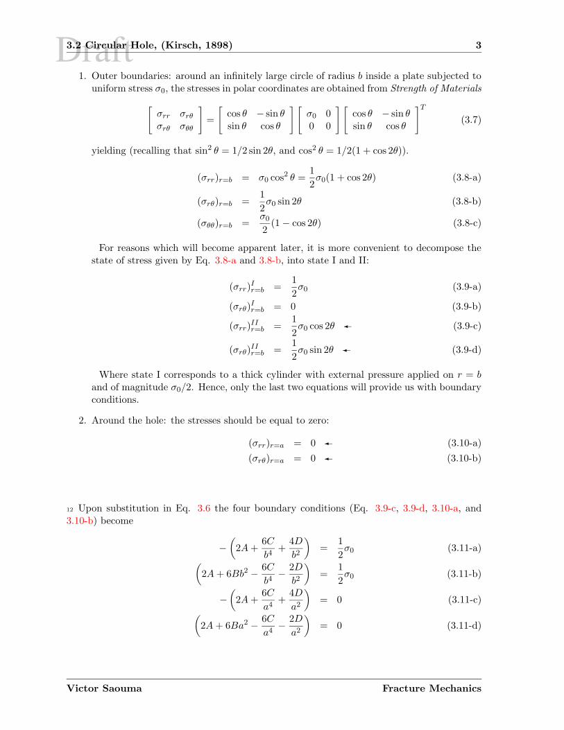
1. Outer boundaries: around an infinitely large circle of radius b inside a plate subjected touniform stress σ0, the stresses in polar coordinates are obtained from Strength of Materials

[

σrr σrθ

σrθ σθθ

]

=

[

cos θ − sin θsin θ cos θ

] [

σ0 00 0

] [

cos θ − sin θsin θ cos θ

]T

(3.7)

yielding (recalling that sin2 θ = 1/2 sin 2θ, and cos2 θ = 1/2(1 + cos 2θ)).

(σrr)r=b = σ0 cos2 θ =1

2σ0(1 + cos 2θ) (3.8-a)

(σrθ)r=b =1

2σ0 sin 2θ (3.8-b)

(σθθ)r=b =σ0

2(1 − cos 2θ) (3.8-c)

For reasons which will become apparent later, it is more convenient to decompose thestate of stress given by Eq. 3.8-a and 3.8-b, into state I and II:

(σrr)Ir=b =

1

2σ0 (3.9-a)

(σrθ)Ir=b = 0 (3.9-b)

(σrr)IIr=b =

1

2σ0 cos 2θ (3.9-c)

(σrθ)IIr=b =

1

2σ0 sin 2θ (3.9-d)

Where state I corresponds to a thick cylinder with external pressure applied on r = band of magnitude σ0/2. Hence, only the last two equations will provide us with boundaryconditions.

2. Around the hole: the stresses should be equal to zero:

(σrr)r=a = 0 (3.10-a)

(σrθ)r=a = 0 (3.10-b)

12 Upon substitution in Eq. 3.6 the four boundary conditions (Eq. 3.9-c, 3.9-d, 3.10-a, and3.10-b) become

−(

2A+6C

b4+

4D

b2

)

=1

2σ0 (3.11-a)

(

2A+ 6Bb2 − 6C

b4− 2D

b2

)

=1

2σ0 (3.11-b)

−(

2A+6C

a4+

4D

a2

)

= 0 (3.11-c)

(

2A+ 6Ba2 − 6C

a4− 2D

a2

)

= 0 (3.11-d)


Draft3.5 V Notch, (Williams, 1952) 17

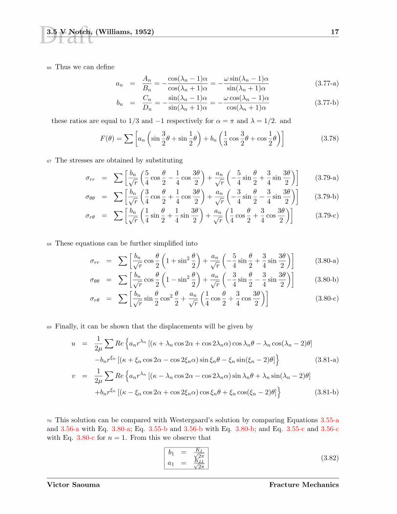
66 Thus we can define

an =An

Bn= −cos(λn − 1)α

cos(λn + 1)α= −ω sin(λn − 1)α

sin(λn + 1)α(3.77-a)

bn =Cn

Dn= −sin(λn − 1)α

sin(λn + 1)α= −ω cos(λn − 1)α

cos(λn + 1)α(3.77-b)

these ratios are equal to 1/3 and −1 respectively for α = π and λ = 1/2. and

F (θ) =∑

[

an

(

sin3

2θ + sin

1

2θ

)

+ bn

(1

3cos

3

2θ + cos

1

2θ

)]

(3.78)

67 The stresses are obtained by substituting

σrr =∑

[bn√r

(5

4cos

θ

2− 1

4cos

3θ

2

)

+an√r

(

−5

4sin

θ

2+

3

4sin

3θ

2

)]

(3.79-a)

σθθ =∑

[bn√r

(3

4cos

θ

2+

1

4cos

3θ

2

)

+an√r

(

−3

4sin

θ

2− 3

4sin

3θ

2

)]

(3.79-b)

σrθ =∑

[bn√r

(1

4sin

θ

2+

1

4sin

3θ

2

)

+an√r

(1

4cos

θ

2+

3

4cos

3θ

2

)]

(3.79-c)

68 These equations can be further simplified into

σrr =∑

[bn√r

cosθ

2

(

1 + sin2 θ

2

)

+an√r

(

−5

4sin

θ

2+

3

4sin

3θ

2

)]

(3.80-a)

σθθ =∑

[bn√r

cosθ

2

(

1 − sin2 θ

2

)

+an√r

(

−3

4sin

θ

2− 3

4sin

3θ

2

)]

(3.80-b)

σrθ =∑

[bn√r

sinθ

2cos2

θ

2+an√r

(1

4cos

θ

2+

3

4cos

3θ

2

)]

(3.80-c)

69 Finally, it can be shown that the displacements will be given by

u =1

2µ

∑

Re

anrλn [(κ+ λn cos 2α+ cos 2λnα) cosλnθ − λn cos(λn − 2)θ]

−bnrξn [(κ+ ξn cos 2α− cos 2ξnα) sin ξnθ − ξn sin(ξn − 2)θ]

(3.81-a)

v =1

2µ

∑

Re

anrλn [(κ− λn cos 2α− cos 2λnα) sinλnθ + λn sin(λn − 2)θ]

+bnrξn [(κ− ξn cos 2α+ cos 2ξnα) cos ξnθ + ξn cos(ξn − 2)θ]

(3.81-b)

70 This solution can be compared with Westergaard’s solution by comparing Equations 3.55-aand 3.56-a with Eq. 3.80-a; Eq. 3.55-b and 3.56-b with Eq. 3.80-b; and Eq. 3.55-c and 3.56-cwith Eq. 3.80-c for n = 1. From this we observe that

b1 = KI√2π

a1 = KII√2π

(3.82)


Draft3.6 Crack at an Interface between Two Dissimilar Materials (Williams, 1959) 19

or F ′1(π) = F ′

2(−π) = 0

• Continuity of σθθ at the interface, θ = 0

A1 +B1 = A2 +B2 (3.87)

• Continuity of σrθ at θ = 0 along the interface

(λ− 1)C1 + (λ+ 1)D1 = −(λ− 1)C2 − (λ+ 1)D2 (3.88)

• Continuity of displacements (ur, uθ) at the interface. Using the polar expression of thedisplacements

uir =

1

2µirλ−(λ+ 1)Fi(θ) + 4(1 − αi)[Ci sin(λ− 1)θ +Ai cos(λ− 1)θ](3.89-a)

uiθ =

1

2µirλ−F ′

i (θ) − 4(1 − αi)[Ci cos(λ− 1)θ −Ai sin(λ− 1)θ] (3.89-b)

where µ is the shear modulus, and αi ≡ νi

1+νi

we obtain

1

2µ1[−(λ+ 1)F1(0) + 4A1(1 − α1)] =

1

2µ2[−(λ+ 1)F2(0) + 4A2(1 − α2)](3.90-a)

1

2µ1

[−F ′

1(0) − 4C1(1 − α1)]

=1

2µ2

[−F ′

2(0) − 4C2(1 − α2)]

(3.90-b)

3.6.3 Homogeneous Equations

74 Applying those boundary conditions, will lead to 8 homogeneous linear equations (Eq. 3.85-a,3.85-b, 3.86-b, 3.86-c, 3.87, 3.88, 3.90-a, 3.90-b) in terms of the 8 unknownsA1, B1, C1, D1, A2, B2, C2

and D2.

75 A nontrivial solution exists if the determinant of the 8 equations is equal to zero. Thisdeterminant5 is equal to

cot2 λπ +

[2k(1 − α2) − 2(1 − α1) − (k − 1)

2k(1 − α2) + 2(1 − α1)

]2

= 0 (3.91)

where k = µ1

µ2.

76 For the homogeneous case α1 = α2 and k = 1, the previous equation reduces to cot2 λπ = 0or sin2 λπ = 0 thus we recover the same solution as the one of Eq. 3.73-b for a crack in onematerial:

λ =n

2n = 1, 2, 3, ... (3.92)

Note that we exclude negative values of n to ensure finite displacements as the origin is ap-proached, and the lowest eigenvalue controls.

5The original paper states: ... After some algebraic simplification...



80 Thus, Eq. 3.91 finally leads to

Re(cotλπ) = 0 (3.100-a)

Im(cotλπ) = ±β (3.100-b)

we thus have two equations with two unknowns.

3.6.4 Solve for λ

81 Let us solve those two equations. Two sets of solutions are possible:

1. If from 3.99-b tanλrπ = 0 then

λr = n = 0, 1, 2, 3, ... (3.101)

and accordingly from Eq. 3.100-b

λj = ± 1

πcoth−1 β (3.102)

2. Alternatively, from Eq. 3.100-a cotλrπ = 0 ⇒ tanλrπ = ∞ and6:

λr =2n+ 1

2n = 0, 1, 2, 3, ... (3.103-a)

λj = ± 1

πtanh−1 β (3.103-b)

=1

2πlog

[β + 1

β − 1

]

(3.103-c)

We note that for this case, λj → 0 as α1 → α2 and k → 1 in β.

3.6.5 Near Crack Tip Stresses

82 Now that we have solved for λ, we need to derive expressions for the near crack tip stressfield. We rewrite Eq. 3.83 as

Φ(r) = rλ+1︸︷︷︸

G(r)

F (θ, λ) (3.104)

we note that we no longer have two sets of functions, as the effect of dissimilar materials hasbeen accounted for and is embedded in λ.

83 The stresses will be given by Eq. ??

σrr =1

r2∂2Φ

∂θ2+

1

r

∂Φ

∂r= r−2G(r)F ′′(θ) + r−1G′(r)F (θ) (3.105-a)

σθθ =∂2Φ

∂r2= G′′(r)F (θ) (3.105-b)

σrθ =1

r2∂Φ

∂θ− 1

r

∂2Φ

∂r∂θ= r−2G(r)F ′(θ) − r−1G′(r)F ′(θ) (3.105-c)

6Recall that tanh−1 x = 12

log 1+x1−x



thus,

Re sin [(λr ± 1) + iλj ] θ = sin(λr ± 1) cos(θ) coshλjθ (3.114-a)

Re cos [(λr ± 1) + iλj ] θ = cos(λr ± 1) cos(θ) coshλjθ (3.114-b)

87 Substituting those relations in Eq. 3.112

Re [F (θ)] = coshλjθ︸︷︷︸

f(θ)

(3.115-a)

[A cos(λr − 1)θ +B cos(λr + 1)θ + C sin(λr − 1)θ +D sin(λr + 1)θ]︸︷︷︸

g(θ)

(3.115-b)

Re [Φ(r, θ)] = rλr+1 cos(λj log(r)) coshλjθ

[A cos(λr − 1)θ +B cos(λr + 1)θ

+C sin(λr − 1)θ +D sin(λr + 1)θ] (3.115-c)

88 For λr = 12

g(θ) = A cosθ

2+B cos

3θ

2− C sin

θ

2+D sin

3θ

2(3.116)

89 Applying the boundary conditions at θ = ±π, σθθ = 0, Eq. 3.105-b F (θ) = 0, that isg1(−π) = g2(π) or

C = −D = −a (3.117)

90 Similarly at θ = ±π, σrθ = 0. Thus, from Eq. 3.105-c F ′(θ) = 0, or g′1(−π) = g′2(π) or

A = 3B = b (3.118)

91 From those two equations we rewrite Eq. 3.116

g(θ) = a

(

sinθ

2+ sin

3θ

2

)

+ b

(

3 cosθ

2+ cos

3θ

2

)

(3.119)

92 We now determine the derivatives

f ′(θ) = λj sinhλjθ (3.120-a)

g′(θ) = a

(3

2cos

3θ

2+

1

2cos

θ

2

)

+ b

(

−3

2sin

3θ

2− 3

2sin

θ

2

)

(3.120-b)

93 Thus, we now can determine

F ′(θ) = f ′(θ)g(θ) + f(θ)g′(θ) (3.121-a)

= a

coshλjθ

[3

2cos

3θ

2+

1

2cos

θ

2

]

+ λj sinhλjθ

[

sin3θ

2+ sin

θ

2

]

+b

coshλjθ

[

−3

2sin

3θ

2− 3

2sin

θ

2

]

+ λj sinhλjθ

[

cos3θ

2+ 3 cos

θ

2

]

(3.121-b)


Draft3.8 Assignment 25

98 where s1 and s2 are roots, in general complex, of Eq. 2.127 where sj = αj + iβj for j = 1, 2,and the roots of interests are taken such that βj > 0, and

pj = a11s2j + a12 − a16sj (3.125)

qj = a12sj +a22

sj− a26 (3.126)

99 After appropriate substitution, it can be shown that the cartesian stresses at the tip of thecrack for symmetric loading are

σx =KI√2πr

Re

[

s1s2s1 − s2

(

s2

(cos θ + s2 sin θ)12

− s1


)]

(3.127-a)

σy =KI√2πr

Re

[

1

s1 − s2

(

s1


− s2


)]

(3.127-b)

σxy =KI√2πr

Re

[

s1s2s1 − s2

(

1


− s1


)]

(3.127-c)

100 and, for plane skew-symmetric loading:

σx =KII√2πr

Re

[

1

s1 − s2

(

s22


− s21


)]

(3.128-a)

σy =KII√2πr

Re

[

1

s1 − s2

(

1


− 1


)]

(3.128-b)

σxy =KII√2πr

Re

[

1

s1 − s2

(

s1


− s2


)]

(3.128-c)

101 For in-plane loadings, these stresses can be summed to give the stresses at a distance r andan angle θ from the crack tip.

102 An important observation to be made is that the form of the stress singularity r−1/2 isidentical to the one found in isotropic solids.

103 It should be noted that contrarily to the isotropic case where both the stress magnitude andits spatial distribution are controlled by the stress intensity factor only, in the anisotropic casethey will also depend on the material elastic properties and the orientation of the crack withrespect to the principal planes of elastic symmetry (through s1 and s2).

3.8 Assignment

CVEN-6831

FRACTURE MECHANICS


Draft3.8 Assignment 27

3. The stress intensity factor of the following problem:

x

x 2

1

a

P

P

B A

a

x

is given by:

KA =P√πa

√

a+ x

a− x(3.130)

Kb =P√πa

√

a− x

a+ x(3.131)

Based on those expressions, and results from the previous problem, determine the stressfunction Φ.

4. Barenblatt’s model assumes a linearly varying closing pressure at the tip of a crack,

c c2(a - c)

σ σy y

Using Mathematica and the expressions of KA and KB from the previous problem, de-termine an expression for the stress intensity factors for this case.

5. Using Mathematica, program either:

(a) Westergaard’s solution for a crack subjected to mode I and mode II loading.

(b) Williams solution for a crack along dissimilar materials.


Draft

Chapter 4

LEFM DESIGN EXAMPLES

1 Following the detailed coverage of the derivation of the linear elastic stress field around a cracktip, and the introduction of the concept of a stress intensity factor in the preceding chapter, wenow seek to apply those equations to some (pure mode I) practical design problems.

2 First we shall examine how is linear elastic fracture mechanics (LEFM) effectively used indesign examples, then we shall give analytical solutions to some simple commonly used testgeometries, followed by a tabulation of fracture toughness of commonly used engineering ma-terials. Finally, this chapter will conclude with some simple design/analysis examples.

4.1 Design Philosophy Based on Linear Elastic Fracture Me-chanics

3 One of the underlying principles of fracture mechanics is that unstable fracture occurs whenthe stress intensity factor (SIF) reaches a critical value KIc, also called fracture toughness. KIc

represents the inherent ability of a material to withstand a given stress field intensity at the tipof a crack and to resist progressive tensile crack extension.

4 Thus a crack will propagate (under pure mode I), whenever the stress intensity factor KI

(which characterizes the strength of the singularity for a given problem) reaches a materialconstant KIc. Hence, under the assumptions of linear elastic fracture mechanics (LEFM), atthe point of incipient crack growth:

KIc = βσ√πa (4.1)

5 Thus for the design of a cracked, or potentially cracked, structure, the engineer would haveto decide what design variables can be selected, as only, two of these variables can be fixed,and the third must be determined. The design variables are:

Material properties: (such as special steel to resist corrosive liquid) ⇒ Kc is fixed.

Design stress level: (which may be governed by weight considerations) ⇒ σ is fixed.

Flaw size: 1, a.

1In most cases, a refers to half the total crack length.

Draft4.2 Stress Intensity Factors 3

Figure 4.2: Single Edge Notch Tension Panel

Figure 4.3: Double Edge Notch Tension Panel

Single Edge Notch Tension Panel (SENT) for LW = 2, Fig. 4.2

KI =

[

1.12 − 0.23

(a

W

)

+ 10.56

(a

W

)2

− 21.74

(a

W

)3

+ 30.42

(a

W

)4]

︸︷︷︸

β

σ√πa (4.4)

We observe that here the β factor for small crack ( aW 1) is grater than one and is

approximately 1.12.

Double Edge Notch Tension Panel (DENT), Fig. 4.3

KI =

[

1.12 + 0.43

(a

W

)

− 4.79

(a

W

)2

+ 15.46

(a

W

)3]

︸︷︷︸

β

σ√πa (4.5)

Three Point Bend (TPB), Fig. 4.4

KI =3√

aW

[

1.99 −(

aW

) (1 − a

W

) (

2.15 − 3.93 aW + 2.7

(aW

)2)]

2(1 + 2 a

W

) (1 − a

W

) 32

PS

BW32

(4.6)

Compact Tension Specimen (CTS), Fig. 4.5 used in ASTM E-399 (399 n.d.) StandardTest Method for Plane-Strain Fracture Toughness of Metallic Materials

KI =

[

16.7 − 104.6

(a

W

)

+ 370

(a

W

)2

− 574

(a

W

)3

+ 361

(a

W

)4]

︸︷︷︸

β

P

BW︸︷︷︸

σ

√πa (4.7)

We note that this is not exactly the equation found in the ASTM standard, but ratheran equivalent one written in the standard form.


Draft

Chapter 5

THEORETICAL STRENGTH ofSOLIDS; (Griffith I)

1 We recall that Griffith’s involvement with fracture mechanics started as he was exploring thedisparity in strength between glass rods of different sizes, (Griffith 1921). As such, he hadpostulated that this can be explained by the presence of internal flaws (idealized as elliptical)and then used Inglis solution to explain this discrepancy.

2 In this section, we shall develop an expression for the theoretical strength of perfect crystals(theoretically the strongest form of solid). This derivation, (Kelly 1974) is fundamentallydifferent than the one of Griffith as it starts at the atomic level.

5.1 Derivation

3 We start by exploring the energy of interaction between two adjacent atoms at equilibriumseparated by a distance a0, Fig. 5.1. The total energy which must be supplied to separate atomC from C’ is

U0 = 2γ (5.1)

where γ is the surface energy1, and the factor of 2 is due to the fact that upon separation, wehave two distinct surfaces.

5.1.1 Tensile Strength

5.1.1.1 Ideal Strength in Terms of Physical Parameters

We shall first derive an expression for the ideal strength in terms of physical parameters, andin the next section the strength will be expressed in terms of engineering ones.

1 From watching raindrops and bubbles it is obvious that liquid water has surface tension. When the surfaceof a liquid is extended (soap bubble, insect walking on liquid) work is done against this tension, and energy isstored in the new surface. When insects walk on water it sinks until the surface energy just balances the decreasein its potential energy. For solids, the chemical bonds are stronger than for liquids, hence the surface energy isstronger. The reason why we do not notice it is that solids are too rigid to be distorted by it. Surface energy γis expressed in J/m2 and the surface energies of water, most solids, and diamonds are approximately .077, 1.0,and 5.14 respectively.

Draft

Chapter 6

ENERGY TRANSFER in CRACKGROWTH; (Griffith II)

1 In the preceding chapters, we have focused on the singular stress field around a crack tip. Onthis basis, a criteria for crack propagation, based on the strength of the singularity was firstdeveloped and then used in practical problems.

2 An alternative to this approach, is one based on energy transfer (or release), which occursduring crack propagation. This dual approach will be developed in this chapter.

3 Griffith’s main achievement, in providing a basis for the fracture strengths of bodies containingcracks, was his realization that it was possible to derive a thermodynamic criterion for fractureby considering the total change in energy of a cracked body as the crack length increases,(Griffith 1921).

4 Hence, Griffith showed that material fail not because of a maximum stress, but rather becausea certain energy criteria was met.

5 Thus, the Griffith model for elastic solids, and the subsequent one by Irwin and Orowan forelastic-plastic solids, show that crack propagation is caused by a transfer of energy transferfrom external work and/or strain energy to surface energy.

6 It should be noted that this is a global energy approach, which was developed prior to theone of Westergaard which focused on the stress field surrounding a crack tip. It will be shownlater that for linear elastic solids the two approaches are identical.

6.1 Thermodynamics of Crack Growth

6.1.1 General Derivation

7 If we consider a crack in a deformable continuum subjected to arbitrary loading, then thefirst law of thermodynamics gives: The change in energy is proportional to the amount of workperformed. Since only the change of energy is involved, any datum can be used as a basis formeasure of energy. Hence energy is neither created nor consumed.

8 The first law of thermodynamics states The time-rate of change of the total energy (i.e., sumof the kinetic energy and the internal energy) is equal to the sum of the rate of work done by

Draft6.1 Thermodynamics of Crack Growth 3

Figure 6.1: Energy Transfer in a Cracked Plate

length 2a located in an infinite plate subjected to load P . Griffith assumed that it was possibleto produce a macroscopical load displacement (P − u) curve for two different crack lengths aand a+ da.

Two different boundary conditions will be considered, and in each one the change in potentialenergy as the crack extends from a to a+ da will be determined:

Fixed Grip: (u2 = u1) loading, an increase in crack length from a to a + da results in adecrease in stored elastic strain energy, ∆U ,

∆U =1

2P2u1 −

1

2P1u1 (6.6)

=1

2(P2 − P1)u1 (6.7)

< 0 (6.8)

Furthermore, under fixed grip there is no external work (u2 = u1), so the decrease inpotential energy is the same as the decrease in stored internal strain energy, hence

Π2 − Π1 = ∆W − ∆U (6.9)

= −1

2(P2 − P1)u1 =

1

2(P1 − P2)u1 (6.10)

Fixed Load: P2 = P1 the situation is slightly more complicated. Here there is both externalwork

∆W = P1(u2 − u1) (6.11)

and a release of internal strain energy. Thus the net effect is a change in potential energygiven by:

Π2 − Π1 = ∆W − ∆U (6.12)


Draft

Chapter 7

MIXED MODE CRACKPROPAGATION

1 Practical engineering cracked structures are subjected to mixed mode loading, thus in generalKI and KII are both nonzero, yet we usually measure only mode I fracture toughness KIc (KIIc

concept is seldom used). Thus, so far the only fracture propagation criterion we have is formode I only (KI vs KIc, and GI vs R).

2 Whereas under pure mode I in homogeneous isotropic material, crack propagation is collinear,in all other cases the propagation will be curvilinear and at an angle θ0 with respect to thecrack axis. Thus, for the general mixed mode case, we seek to formulate a criterion that willdetermine:

1. The angle of incipient propagation, θ0, with respect to the crack axis.

2. If the stress intensity factors are in such a critical combination as to render the cracklocally unstable and force it to propagate.

3 Once again, for pure mode I problems, fracture initiation occurs if:

KI ≥ KIc (7.1)

4 The determination of a fracture initiation criterion for an existing crack in mode I and IIwould require a relationship between KI,KII, and KIc of the form

F (KI,KII,KIc) = 0 (7.2)

and would be analogous to the one between the two principal stresses and a yield stress, Fig.7.1

Fyld(σ1, σ2, σy) = 0 (7.3)

Such an equation may be the familiar von Mises criterion.

5 In the absence of a widely accepted criterion for mixed mode crack growth, three of the mostwidely used criterion are discussed below.

Draft7.1 Analytical Models for Isotropic Solids 3

Solution of the second equation yields the angle of crack extension θ0

tanθ02

=1

4

KI

KII± 1

4

√(KI

KII

)2

+ 8 (7.8)

10 For the crack to extend, the maximum circumferential tensile stress, σθ (from Eq. 3.55-band 3.56-b)

σθ =KI√2πr

cosθ02

(

1 − sin2 θ02

)

+KII√2πr

(

−3

4sin

θ02

− 3

4sin

3θ02

)

(7.9)

must reach a critical value which is obtained by rearranging the previous equation

σθmax

√2πr = KIc = cos

θ02

[

KI cos2θ02

− 3

2KII sin θ0

]

(7.10)

which can be normalized as

KI

KIccos3

θ02

− 3

2

KII

KIccos

θ02

sin θ0 = 1 (7.11)

11 This equation can be used to define an equivalent stress intensity factor Keq for mixed modeproblems

Keq = KI cos3θ02

− 3

2KII cos

θ02

sin θ0 (7.12)

7.1.2 Maximum Energy Release Rate

12 In their original model, Erdogan, F. and Sih, G.C. (1963) noted that:

“If we accept Griffith (energy) theory as the valid criteria which explains crackgrowth, then the crack will grow in the direction along which the elastic energyrelease per unit crack extension will be maximum and the crack will start to growwhen this energy reaches a critical value (or G = G(δ, θ)). Evaluation of G(δ, θ)poses insurmountable mathematical difficulties.”

13 Finding G(δ, θ) will establish for the general mixed mode case the duality which is the basisof fracture mechanics: the equivalence in viewing fracture initiation from either a global energybalance or a local stress intensity point of view.

14 This (insurmountable) problem was solved in 1974, by Hussain et al. (1974). Fundamen-tally, Hussain et al. (1974) have solved for the stress intensity factor of a major crack with aninfinitesimal “kink” at an angle θ, KI(θ) and KII(θ) in terms of the stress intensity factors ofthe original crack KI and KII , Fig. 7.2:

KI(θ)KII(θ)

=

(4

3 + cos2 θ

)(

1 − θπ

1 + θπ

) θ2π

KI cos θ + 32KII sin θ

KII cos θ − 12KI sin θ

(7.13)


Draft

Part II

ELASTO PLASTIC FRACTUREMECHANICS

Draft

Chapter 8

PLASTIC ZONE SIZES

1 it was shown in chapter ?? that, under linear elastic fracture mechanics assumptions, thestress at the crack tip is theoretically infinite. Clearly, all materials have a finite strength, thusthere will always be a small plastified zone around the crack tip.

2 If this zone is small compared to the crack size, then our linear elastic assumptions are correct;if not, LEFM is not applicable (thus it would be incorrect to use a K or G criterion) and anonlinear model must be used. This “damaged” zone is referred to as a plastic zone for metals,and a fracture process zone for cementitious materials and ceramics.

3 Thus there are two important issues associated with nonlinear fracture:

1. What is the size of the plastic or process zone?

2. What are the criteria for crack growth?

4 This chapter will answer the first question by focusing on metals1, whereas the next chapterwill develop criterions for crack growth.

5 The evaluation of the plastic zone for plastified materials can be determined through variouslevels of approximations:

1. Uniaxial stress criteria

(a) first order approximation

(b) second order approximation (Irwin)

(c) Dugdale’s model

2. Multiaxial yield criteria

Each one of them will be separately reviewed.

8.1 Uniaxial Stress Criteria

6 First we shall examine criteria in which only the uniaxial stress state (σyy normal to theecrack axis) and we shall consider three models of increasing complexities.

1Due to the intrinsically different behavior of concrete compared to metals, estimates of the fracture processzone will be separately discussed.

Draft8.1 Uniaxial Stress Criteria 3

Figure 8.2: Second-Order Approximation of the Plastic Zone

=

∫ r∗p

0σ

√a

2r−

12 dr − σyldr

∗p

= σ

√a

22r

12 |r

∗

p

0 −σyldr∗p

= σ√

2ar∗p − σyldr∗p (8.5)

9 Equating A to B we obtain:

σ√

2ar∗p − σyldr∗p = σyldδ

σyld(δ + r∗p) = σ√

2ar∗p

(δ + r∗p)2 =

2aσ2

σ2yld

r∗p (8.6)

10 From Eq. 8.3, r∗p = a2

(σ

σyld

)2, thus this simplifies into

δ + r∗p = 2r∗p ⇒ δ = r∗p (8.7)

rp = 2r∗p (8.8)

rp =1

π

KI

σ2yld

=

(σ

σyld

)2

a (8.9)

11 Note that rp = 2r∗p and that we can still use r∗p but with aeff = a+ r∗p; thus we can consideran effective crack length of a+ r∗p which would result in:

Keff = f(g)σ√

π(a+ r∗p) = f(g)σ

√

π(a+K2

2πσ2yld

) (8.10)


Draft8.1 Uniaxial Stress Criteria 5

Figure 8.3: Dugdale’s Model

Figure 8.4: Point Load on a Crack


Draft8.2 Multiaxial Yield Criteria 7

Figure 8.6: Barenblatt’s Model

8.2 Multiaxial Yield Criteria

24 All the previous models have restricted themselves to θ = 0 and have used uniaxial yieldcriteria, but the size of the plastic zone can be similarly derived from a multi-axial yield criterion.

25 The principal stresses at a point with respect to the crack tip are given by:

σ1,2 =σx + σy

2±√(σx − σy

2

)2

+ τ2xy (8.24)

where the stresses were obtained in Eq. 3.52-a, 3.52-b, and 3.52-c

σ1 =KI√2πr

cosθ

2

[

1 + sinθ

2

]

(8.25)

σ2 =KI√2πr

cosθ

2

[

1 − sinθ

2

]

(8.26)

σ3 = ν(σ1 + σ2) (8.27)

for plane strain, orσ3 = 0 (8.28)

for plane stress.

26 With those stress expressions, any yield criteria could be used. Using the von Mises criteria,we would obtain:

σe =1√2

[

(σ1 − σ2)2 + (σ2 − σ3)

2 + (σ3 − σ1)2] 1

2 (8.29)

and yielding would occur when σe reaches σyld. Substituting the principal stresses (with r = rp)into this equation and solving for rp yields

• For plane strain:

rp(θ) =1

4π

KI

σ2yld

[3

2sin2 θ + (1 − 2ν)2(1 + cos θ)

]

(8.30)


Draft8.3 Plane Strain vs. Plane Stress 9

Figure 8.8: Plastic Zone Size Across Plate Thickness

31 We also observe that since rp is proportional to(

KI

σyld

)2, the plate thickness should increase

as either the SIF increase or the yield stress decrease.

32 Furthermore, the different stress fields present at the tip of the crack under plane stress andplane strain will result in different deformation patterns. This is best explained in terms of theorientation of the planes of maximum shear stress for both cases, Fig. 8.9.

Plane Stress: σz = 0, and the maximum shear stress τmax is equal to σx

2 and occurs atapproximately 45 degrees from the crack plane.

Plane Strain: In this case we have σy < σz < σx, and the maximum shear stress is equal toσx−σy

2 which is not only much smaller than σx

2 but occurs on different planes.

33 Finally, it should be noted, once again, that fracture toughness KIc can only be measuredunder plane strain conditions, Fig. 8.10


Draft

Chapter 9

FATIGUE CRACKPROPAGATION

1 When a subcritical crack (a crack whose stress intensity factor is below the critical value) issubjected to either repeated or fatigue load, or is subjected to a corrosive environment, crackpropagation will occur.

2 As in many structures one has to assume the presence of minute flaws (as large as the smallestone which can be detected). The application of repeated loading will cause crack growth. Theloading is usually caused by vibrations.

3 Thus an important question that arises is “how long would it be before this subcritical crackgrows to reach a critical size that would trigger failure?” To predict the minimum fatigue lifeof metallic structures, and to establish safe inspection intervals, an understanding of the rateof fatigue crack propagation is required.

Historically, fatigue life prediction was based on S − N curves, Fig. 9.1 (or Goodman’s

Figure 9.1: S-N Curve and Endurance Limit

Diagram) using a Strength of Material Approach which did NOT assume the presence of acrack.

9.1 Experimental Observation

4 If we start with a plate that has no crack and subject it to a series of repeated loading, Fig.9.2 between σmin and σmax, we would observe three distinct stages, Fig. 9.3

1. Stage 1 : Micro coalescence of voids and formation of microcracks. This stage is difficultto capture and is most appropriately investigated by metallurgists or material scientists,

Draft9.2 Fatigue Laws Under Constant Amplitude Loading 3

law based on experimental observations. Most other empirical fatigue laws can be consideredas direct extensions, or refinements of this one, given by

da

dN= C (∆K)n (9.1)

which is a straight line on a log-log plot of dadN

vs ∆K, and

∆K = Kmax −Kmin = (σmax − σmin)f(g)√πa (9.2)

a is the crack length; N the number of load cycles; C the intercept of line along dadN

and is of

the order of 10−6 and has units of length/cycle; and n is the slope of the line and ranges from2 to 10.

10 Equation 9.1 can be rewritten as :

∆N =∆a

C [∆K(a)]n(9.3)

or

N =

∫

dN =

∫ af

ai

da

C [∆K(a)]n(9.4)

11 Thus it is apparent that a small error in the SIF calculations would be magnified greatlyas n ranges from 2 to 6. Because of the sensitivity of N upon ∆K, it is essential to properlydetermine the numerical values of the stress intensity factors.

12 However, in most practical cases, the crack shape, boundary conditions, and load are in sucha combination that an analytical solution for the SIF does not exist and large approximationerrors have to be accepted. Unfortunately, analytical expressions forK are available for only fewsimple cases. Thus the stress analyst has to use handbook formulas for them (Tada et al. 1973).A remedy to this problem is the usage of numerical methods, of which the finite element methodhas achieved greatest success.

9.2.2 Foreman’s Model

13 When compared with experimental data, it is evident that Paris law does not account for:

1. Increase in crack growth rate as Kmax approaches KIc

2. Slow increase in crack growth at Kmin ≈ Kth

thus it was modified by Foreman (Foreman, Kearney and Engle 1967), Fig. 9.4

da

dN=

C(∆K)n

(1 −R)Kc − ∆K(9.5)

9.2.3 Modified Walker’s Model

14 Walker’s (Walker 1970) model is yet another variation of Paris Law which accounts for thestress ratio R = Kmin

Kmax= σmin

σmax

da

dN= C

[∆K

(1 −R)(1−m)

]n

(9.6)


Draft9.3 Variable Amplitude Loading 5

aluminum which has R = 15 kJ/m2 E = 70 GPa C = 5 × 10−11 m/cycle, and n = 3. Thesmallest detectable flaw is 4 mm. How long would it be before the crack will propagate to itscritical length?

Assuming K = σ√πa and Kc =

√ER, then ac = K2

c

σ2maxπ

= ERσ2

maxπor

ac =(70 × 109)(15 × 103)

(200 × 106)2π= 0.0084m = 8.4mm (9.8)

⇒ N =

∫ af

ai

da

C[∆K(a)]n=

∫ af

ai

da

C (σmax − σmin)n

︸︷︷︸

(∆σ)n

((πa)12 )n

=

∫ 8.4×10−3

4×10−3

da

(5 × 10−11)︸︷︷︸

C

(200 − 50)3︸︷︷︸

(∆σ)3

(πa)1.5

︸︷︷︸

((πa).5)3

= 1064

∫ .0084

.004a−1.5da

= −2128a−.5 |.0084.004 = 2128[− 1√.0084

+ 1√.004

]

= 10, 428 cycles

(9.9)

thus the time t will be: t = (10,428) cycles × 110

flightcycle ×1

2day

flight × 130

monthday ≈ 17.38 month

≈ 1.5 years.If a longer lifetime is desired, then we can:

1. Employ a different material with higher KIc, so as to increase the critical crack length ac

at instability.

2. Reduce the maximum value of the stress σmax.

3. Reduce the stress range ∆σ.

4. Improve the inspection so as to reduce the assumed initial crack length amin.

9.2.6.2 Example 2

21 Repeat the previous problem except that more sophisticated (and expensive) NDT equipmentis available with a resolution of .1 mm thus ai = .1mm

t = 2128[− 1√.0084

+ 1√.0001

] = 184, 583 cycles

t = 173810,428(189, 583) = 316 months ≈ 26 years!

9.2.6.3 Example 3

Rolfe and Barsoum p.261-263.

9.3 Variable Amplitude Loading

9.3.1 No Load Interaction

22 Most Engineering structures are subjected to variable amplitude repeated loading, however,most experimental data is based on constant amplitude load test. Thus, the following questionsarise:


Draft

Chapter 10

CRACK TIP OPENINGDISPLACEMENTS

1 Within the assumptions and limitations of LEFM we have two valid (and equivalent) criteriafor crack propagation: 1) K vs KIc which is a local criteria based on the strength of the stresssingularity at the tip of the crack; and 2) G vs GIc (or R) which is a global criteria based onthe amount of energy released (or consumed) during a unit surface crack’s propagations.

2 In many cases it is found that LEFM based criteria is either: too conservative and expensiveas it does not account for plastification at the crack tip, and/or invalid based on calculationsof r∗p where LEFM assumptions are checked.

3 Thus, in those cases where LEFM is not applicable, an alternative criteria for crack growthin Elasto Plastic Fracture Mechanics (EPFM) is sought.

4 But first let us note the various stages of ductile fracture:

1. Blunting of an initially sharp crack. Under LEFM assumptions, the crack tip openingdisplacement (CTOD) is zero, however in elasto-plastic material due to blunting it isdifferent from zero, Fig. 10.1.

Figure 10.1: Crack Tip Opening Displacement, (Anderson 1995)

2. Crack initiation

3. Slow (stable) crack growth

4. Unstable crack growth

Draft10.1 Derivation of CTOD 3

v =KI

2µ

[r

2π

] 12

sinθ

2

[

κ+ 1 − 2 cos2θ

2

]

(10.1)

11 If we substitute θ = ±π we obtain the upper and lower displacements of the crack face, anddue to symmetry their sum corresponds to the crack opening displacement. Hence the crackopening is given by

COD = 2v =κ+ 1

µKI

√r

2π(10.2)

12 If we determine the crack tip opening displacement a distance r∗p away from the crack tipusing Irwin’s plastic zone correction from Eq. 8.9

r∗p =1

2π

K2I

σ2yld

(10.3)

and using κ = 3−ν1+ν for plane stress we obtain

CTOD =4

π

K2I

Eσyld

(10.4)

10.1.2 Dugdale’s Solution

13 Using Dugdale’s solution, Kanninen (Kanninen 1984) has shown that the crack opening alongthe crack is given by1:

v(x) =2

π

aσyld

E

log

∣∣∣∣∣

√c2 − a2 +

√c2 − x2

√c2 − a2 −

√c2 − x2

∣∣∣∣∣+x

alog

∣∣∣∣∣

x√c2 − a2 + a

√c2 − x2

x√c2 − a2 − a

√c2 − x2

∣∣∣∣∣

(10.5)

for 0 ≤ x ≤ c. For x = a this reduces to

v(a) =4

π

aσyld

Elog

c

a(10.6)

14 Combining this equation with Dugdale’s solution for c from Eq. 8.21,

a

c= cos

π

2

σ

σyld

(10.7)

we would then obtain

CTOD = 2v =8

π

aσyld

Elog

[

secπ

2

σ

σyld

]

(10.8)

15 using the series expansion of log sec:

CTOD =8

π

aσyld

E

[

1

2

(π

2

σ

σyld

)2

+1

12

(π

2

σ

σyld

)4

+ · · ·]

(10.9)

or

CTOD =K2

Eσyld

[

1 +π2

24

σ2

σ2yld

+ . . .

]

(10.10)

note that for small σσyld

, the CTOD can be approximated by CTOD = K2

Eσyld.

1Derivation of this equation can be found on p. 203 of (Anderson 1995)


Draft

Chapter 11

J INTEGRAL

11.1 Genesis

1 Eshelby (Eshelby 1974) has defined a number of contour integrals that are path independentby virtue of the theorem of energy conservation. The two-dimensional form of one of theseintegrals can be written as:

J =

∮

Γ

(

wdy − t∂u

∂xdy

)

= 0 (11.1)

with

w =

∫ ε

0σijdεij (11.2)

where w is the strain energy density; Γ is a closed contour followed counter-clockwise, as shownin Fig. 11.1; t is the traction vector on a plane defined by the outward drawn normal n andt = σn; u the displacement vector, and dy is the element of the arc along the path Γ.

x

y

ΓΩ

ut ds

ds

Figure 11.1: J Integral Definition Around a Crack

2 Whereas Eshelby had defined a number of similar path independent contour integrals, he hadnot assigned them with a particular physical meaning.

Draft11.3 Nonlinear Elastic Energy Release Rate 3

9 Thus the integrand of Eq. 11.3 vanishes and J = 0 for any closed contour.

10 Having shown that indeed J = 0, we will now exploit this to proove that around a crack, Jis non-zero and is independent of the path.

11 With reference to Fig. 11.2 if we consider the closed path Γ = Γ1 +Γ2 +Γ3 +Γ4 in which Γ1

and Γ3 are arbitrarily chosen contours. Obviously J = 0 over Γ in order to satisfy compatibilityconditions, provided that the stresses and displacement gradients are continuous. Along pathsΓ2 and Γ4, the traction vector ti = 0 and also dy = 0. Consequently, the contributions to Jfrom Γ2 and Γ4 vanish. Taking into account the difference sense of integration along pathsΓ1 and Γ3 we arrive at the conclusion that the values of J integrated over paths Γ1 and Γ3

are identical. Because these two paths were arbitrarily chosen, the path independence of J isassured.

Γ1Γ

ΓΓ3

2

4x

y

Figure 11.2: Closed Contour for Proof of J Path Independence

11.3 Nonlinear Elastic Energy Release Rate

12 Let us now establish the connection between the two previous interpretations of J , the onemathematically defined by Eshelby, and the one associated with the energy release rate (yetto be proven). We shall prove that when J is applied along a contour around a crack tip, itrepresents the change in potential energy for a virtual crack extension da. Two slightly differentderivations are presented.

11.3.1 Virtual Crack Extension

13 Considering a two-dimensional crack surrounded by a line Γ which encompasses an area Ω.Under quasi-static conditions, and in the absence of body forces, the potential energy is givenby

Π =

∫

ΩwdΩ −

∮

Γtiuidy (11.12)

14 For a virtual crack extension, the change in potential energy is

dΠ

da=

∫

Ω

dw

dadΩ −

∮

Γ

[

tidui

da+ ui

dtida

]

dy (11.13-a)


Draft

Part IV

FRACTURE MECHANICS OFCONCRETE

Draft

Chapter 12

FRACTURE DETERIORATIONANALYSIS OF CONCRETE

12.1 Introduction

1 It is ironic that although the foundation for fracture mechanics was laid by Griffith in theearly thirties for brittle materials (such as concrete) (Griffith 1921), it has been mostly appliedto metallic materials. Although there have been some pioneering efforts to apply fracturemechanics to concrete (Kaplan 1961), it was not until the mid-seventies that a number ofresearchers from the academic community focused their attention on various aspects of thisapplication.

2 In applying fracture mechanics to concrete, much was initially borrowed from the wealth ofinformation and research previously undertaken in conjunction with metals by metallurgists ormechanical engineers. However, it quickly became evident that by its very heterogeneous natureconcrete has some unique fracture characteristics, which required the alteration of existingmodels.

3 By now fracture mechanics is universally acknowledged as a viable tool of analysis for in-vestigation of concrete cracking. And after many years of development on numerous (plastic-ity based) constitutive models for concrete, tensile cracking remains its undisputed “Achille’sheel”. For the most part, even the simplest constitutive models appear to perform reasonablywell under compressive regimes, however their capabilities are seriously challenged under tensilestresses. This apparent inability to properly model tensile cracking is of minor importance inreinforced concrete structures in which the steel “takes over” the tensile stresses.

4 However for unreinforced structures, such as dams, the apparent inability of the constitutivemodels to properly and efficiently model tensile cracking is a major handicap. As such forunreinforced concrete structures prone to tensile cracking, a fracture mechanics based model(rather than a plasticity based one) should be used.

5 Whereas an inappropriately large number of papers have been published on computationalmodels for concrete (some of which will be discussed in a separate chapter), relatively fewresearch has been undertaken to properly understand and characterize fracture models. Hence,this chapter will exclusively focus on the phenomenological aspects of concrete fracture from amaterial point of view.

Draft12.2 Phenomenological Observations 3

(not necessarily corresponding to the loading direction). To accomplish this test a clipgage or a strain gage has to provide the feedback signal to the testing equipment in orderto accordingly adjust the stroke.

10 Most concrete fracture tests are conducted under strain control with a gage located at themouth of the crack providing the specimen response.

11 Both stroke and strain controlled tests require a closed-loop experimental set up, which isusually expensive and was not widely available until very recently.

12.2.2 Pre/Post-Peak Material Response of Steel and Concrete

12 As an introduction to concrete fracture, let us compare the pre- and post-peak response ofmetals and concrete, as illustrated in Fig.12.2, both obtained in a strain-controlled test of anuncracked or un-notched specimen.

ε

σ σ

ε ε

Steel Concrete

.1% .01%.2% 25%

f’

.6f’c

c

Figure 12.2: Stress-Strain Curves of Metals and Concrete

1. Pre-peak:

(a) Metal exhibits a linear elastic response up to the yield stress σyld, and an approximatestrain of 0.1%. Subsequently, due to internal dislocation plastic deformation withstrain up to 25% may result to be followed by strain hardening.

(b) Concrete exhibits a linear response up to approximately 0.6f ′t . Subsequently, internal

microcracking induces a nonlinear response up to a peak stress f ′t and a corresponding

strain of approximately 0.01%.

Under load control only the pre-peak response can be measured.

2. Post-peak:

(a) Metals response in the post-peak zone is not yet well understood. Not only is it notof practical usefulness, but also it is largely overshadowed by necking.

(b) Concrete response in the post-peak zone is most interesting, as it can exhibit addi-tional strains. The descending branch of the concrete response in Fig. 12.2 is anidealization of the average material response. A more accurate description shouldaccount for the localization of the induced cracks. Thus away from the localizedcrack there is an elastic unloading, and at the crack, since a strain cannot be prop-erly defined, a stress-crack opening displacement is a more appropriate model. Thiswill be discussed in the subsequent section.


Draft12.3 Localisation of Deformation 5

12.3.1.1 σ-COD Diagram, Hillerborg’s Model

19 From the previous discussion, it is clear that concrete softening is characterized by a stress-crack opening width curve (and not stress-strain). The exact charachterization of the softeningresponse should ideally be obtained from a uniaxial test of an uncracked specimen. However,it has been found (Li and Liang 1986, Hordijk, Reinhardt and Cornelissen 1989) that notonly are those tests extremely sensitive, but drastically different results can be obtained fromdifferent geometries, sizes, and testing machines. Hence, the softening curve is often indirectlydetermined by testing notched specimens.

20 In what is probably the most referenced work in the nonlinear fracture of concrete literature,Hillerborg (Hillerborg, A. and Modeer, M. and Petersson, P.E. 1976) presented in 1976 a verysimple and elegant model which has been previously described qualitatively. In this model, thecrack is composed of two parts, Fig. 12.4:

Figure 12.4: Hillerborg’s Fictitious Crack Model

1. True or physical crack across which no stresses can be transmitted. Along this zone wehave both displacement and stress discontinuities.

2. Fictitious crack, or Fracture Process Zone (FPZ) ahead of the previous one, characterizedby:

(a) peak stress at its tip equal to the tensile strength of concrete

(b) decreasing stress distribution from f ′t at the tip of the fictitious crack to zero at thetip of the physical crack

It should be noted that along the FPZ, we have displacement discontinuity and stresscontinuity.


Draft13.1 Linear Elastic Fracture Models 3

13.1.2 Testing Procedure

10 Fracture toughness tests should be conducted under strain control where the strain is ameasure of the crack mouth opening displacement2 in a servo-controlled manner, Fig. 13.1.

Figure 13.1: Servo-Controlled Test Setup for Concrete KIc and GF

11 During the test, a plot of the load versus crack mouth opening displacement should beobserved, Fig. 13.2.

12 The CMOD is first gradually increased. Following a linear part, a nonlinear prepeak responseis first observed. This is associated with slow crack growth and thus the formation of a FPZturning the notch into a crack. At around the peak load, the CMOD is decreased, thus effectivelyreducing the load. The load is then reapplied and the response would then extend into the post-peak regime. Throughout the descending branch of the structural softening, a series of unloadand reload is performed in order to determine the experimental compliance of the crackedspecimen for different crack lengths3.

13.1.3 Data Reduction

Effective Young’s modulus The effective crack length determination entails measurementof the specimen compliance (inverse of the stiffness or displacement over load). Thecompliance determination in turn requires the concrete Young’s modulus.

The elastic modulus can be determined from:

2 To conduct such tests under displacement control might result in undesirable snapbacks if the testingequipment is not rigid enough.

3Unload reload are not required for the experimental determination of GF as this would simply be the areaunder the P-CMOD curve.


Draft13.2 Nonlinear Fracture Models 5

Figure 13.3: Effective Crack Length Definition

Compliance Derivative Method If the SIF were not derived from the finite elementanalysis, than the Compliance Derivative Method can be used to determine them.Recalling from Eq. 6.31 we have:

G =P 2

2B

∂C

∂a(13.6)

where P, a, C, and B are the applied load, crack length, compliance, and specimen

width respectively. Combining Eq. 13.6 with G =K2

I

E′ where E′ = E for plane stressand E′ = E

1−µ2 for plane strain, we obtain:

KI =E′P 2

2B

∂C

∂a(13.7)

Recalling that the experimental compliance is related to the normalized one throughCn = ECexp, and assuming plane stress condition, Eq. 13.7 can be rearranged into:

KI =P 2

2B

∂Cn

∂a(13.8)

This apparently simple and “elegant” method calls has a major drawback. Since thecompliance is numerically approximated by Eq. 13.4, its derivative is very likely tobe a very poor numerical approximation resulting in gross error when Eq. 13.8 isdetermined.

In summary, the initial unload reload will give Eeff , and each subsequent one will givea KIc corresponding to a different crack length. Thus more than one fracture toughnessvalue can be obtained from a test whereas only one value of GF can be obtained.

13.2 Nonlinear Fracture Models

13.2.1 Hillerborg Characteristic Length

13 The characteristic length, lch, proposed by Hillerborg (Hillerborg, A. and Modeer, M. andPetersson, P.E. 1976) in 1976 is a material property which gives an indication of the material


Draft13.2 Nonlinear Fracture Models 7

16 Thus in this simple, clear, and elegant model we implicitly account for softening by in-troducing a second parameter (CTOD), whereas in Hillerborg’s approach the SIF concept isentirely discarded and replaced by a fictitious load, the distribution of which requires at leasttwo parameters.

17 This model has been shown to yield results that are specimen size insensitive. A minordrawback of this model is that it requires an analytical expression of the COD and KI alongthe crack for the geometry considered. In most cases this entails a finite element calibration.

18 This model requires an analytical expression for KI and the CTOD along the crack foreach geometry considered, which in most cases can only be obtained through a finite elementcalibration. The model distinguishes between notch and crack length, and CTODc is evaluatedat the notch, thus the nonzero value for CTODc. Based on an extensive test program, thecritical values, KS

Ic and CTODc, were found to be size-independent material properties.

19 Finally, when combined with Young’s Modulus, E, a single fracture parameter describingthe material, termed the critical material length, Q, was derived:

Q =

(

E · CTODc

KSIc

)2

(13.13)

The Q-value is related to the brittleness of the specimen. For large Q-values the materialexhibits a high brittleness.

13.2.3 Size Effect Law, Bazant

Refer to chapter 14.

13.2.4 Carpinteri Brittleness Number

20 In fracture testing, failure may be caused by different mechanisms: (1) ultimate strengthcollapse (SOM), and, (2) fracture collapse in terms of LEFM. The dimensionless brittlenessnumber, s, was developed by Carpinteri to assess the existence of either one of the two failuremechanisms (Carpinteri 1982a), (Carpinteri 1982b), (Carpinteri 1986). This parameter dependson the fracture toughness, KIc, the tensile strength, f ′t , and on a dimension d characteristic ofthe specimen (or structure) geometry being considered:

s =KIc

f ′t√d

(13.14)

21 For large brittleness numbers, i.e., small specimen dimension d, SOM governs, and the in-terpretation of tests through Fracture Mechanics (FM) is not valid. Conversely, for smallbrittleness numbers, fracture mechanics is applicable since the specimen is more brittle. Theboundary between SOM and FM applicability, is defined by the critical brittleness number, s0,which is obtained from the nominal stress at failure.


Draft13.3 Comparison of the Fracture Models 9

13.3.2 Bazant Brittleness Number, β

27 The intersection between the SOM and LEFM approaches in the size effect diagram (Fig.14.10) where

σLEFMN = σSOM

N (13.20)

defines the point where the brittleness number, β is equal to 1, or d = λ0da = d0. From

KIc = DPmax

t · d√d (13.21)

Pmax

td=

KIc

D√d0

(13.22)

and combining withPmax

t · d =σN

C(13.23)

we obtainPmax

td=Bf ′tC

(13.24)

Eqs. 13.22 and 13.24 are combined into one equation, yielding:

f ′t2d0

K2Ic

=

(C

BD

)2

= K2 (13.25)

28 Because LEFM is assumed valid, substituting K2Ic with GF · E (Eq. 13.16), leads to:

f ′t2d0

GFE=d0

lch= K2 (13.26)

29 Thus, the brittleness number β used to assess the applicability of LEFM in the Size EffectLaw can be related to Hillerborg’s characteristic length, lch. Eq. 13.26 indicates that d/lch has asimilar significance to the ratio between structural dimension d and maximum aggregate size da

in the Size Effect Law. Since lch is a comprehensive parameter to describe material fracture, thed/da ratio in the Size Effect Law may be replaced by d/lch (Bruhwiler, E., 1988). Comparisonbetween the Size Effect Law and the Fictitious Crack Model showed that both models yieldgood agreement in the prediction of the size effect (Hillerborg, A. 1985b) and (Bazant 1985).

13.3.3 Carpinteri Brittleness Number, s

30 Squaring the expression s of the brittleness number (Eq. 13.14), and assuming that K2Ic =

E ·GF , when LEFM is valid, the following expression is obtained:

s2 =EGF

f ′t2d

=lchd

(13.27)

or

s =

√

lchd

(13.28)


Draft13.4 Model Selection 11

1. Crack size: In a “large” crack, the effect of the process zone is smaller than for a “short”one. Thus LEFM is more applicable for the large ones.

2. Type of loading: If a structure is subjected to a load rather than imposed displacements(such as foundation settlements), than only a pre-peak response is of importance. Underthose conditions non-linear effects may be negligible compared to the ones induced byLEFM.

3. Stability5: In a structure subjected to imposed load rather than imposed displacementnon-linear effects are not be as negligible in a stable structure as they are in an unstableone.

Thus Table 13.2 provides some guidance for model selection. Accordingly we should select:

1. An NLFM for an arch dam which cracking is caused by foundation settlement.

2. An LEFM model for a dam in which cracking is caused by flooding, no matter how smallor large the crack is.

Loading “Small” Crack “Large” Crack

Load Control, Unstable LEFM LEFMLoad Control, Stable NLFM LEFM

Displacement Control NLFM LEFM

Table 13.2: When to Use LEFM or NLFM Fracture Models

34 In all cases, it should be emphasized that ideally a non-linear analysis is to be undertaken,however in many (but not all) cases the complexity and expenses associated with such ananalysis yield results very close to the ones obtained from a linear elastic ones. Thus ultimatelythe type of analysis to be undertaken hinges on both technical and economical considerations.

5A stable structure is one in which KI decreases with crack length, in an unstable one the stress intensityfactor KI increases with crack length.


Draft

Chapter 14

SIZE EFFECT

Paper in print

1 Crack bridging occurs when cohesive stresses join the opposite faces of a crack, shielding thetip from the full effect of the applied load and thus giving rise to increased fracture resistance.Cohesive stresses are present both in elasto-plastic materials such as metals (through cracktip yielding), (Dugdale 1960), (Barenblatt 1962) and in quasi-brittle ones. In the later, theyare present not only in cementitious materials, but also in ceramics, (Saouma, Natekar andSbaizero 2002) and are caused by reinforcing fibers, particles (such as aggregates or inclusions),or simply regions of microscopically irregular crack surfaces causing topological interference.

2 Cohesive stress models were first suggested by Dugdale (1960) using a constant stress, thenBarenblatt (1962) generalized this concept to a more general stress distribution, one whichcauses the crack faces to close smoothly. It should be noted that those two pioneering studiesattributed different causes to the cohesive stresses. For Dugdale it was caused by macroscopicplasticity (and can be of any size) while for Barenblatt it was caused by molecular cohesion (andmust be restricted to a relatively very small zone), (Kanninen and Popelar 1985). Finally, mostrecently Hillerborg, A. and Modeer, M. and Petersson, P.E. (1976) assumed a nonlinear modelwhere the stress is a function of the crack opening. The first two models are most appropriatefor metals to account for the presence of a plastic zone, whereas Hillerborg’s model is moresuited for cementitious material with a fracture process zone.

3 In both Dugdale and Barenblatt solution, the stress intensity factors caused by the far fieldload, and the cohesive stresses are assumed to cancel each other. Hence, implicit in this as-sumption is a zero material fracture toughness.

4 Finally, Hillerborg does not consider any singularity at the tip of the crack. Implicit in hisapproach is that there can not be a stress singularity at the crack tip since the criterion for crackpropagation is based on the crack tip stress. This assumption was recently challenged by Xuand Reinhardt (1998) who developed the double-K criterion where KR(∆a) = Kini

Ic +KC(∆a)and KC(∆a) = F (ft, f(σ),∆a). In this model, developed for concrete, the resistance to crackgrowth (right hand side) is first set to the inherent toughness, and then to a cohesive term.Hence, contrarily to Hillerborg’s model, a cohesive stress does not necessarily eliminate thestress singularity, and as such crack propagation is no longer governed by a stress criteria, butrather by a modified linear elastic fracture mechanics one. This model enables us to distinguishbetween initial crack growth (in the absence of a fracture process zone) governed by K ini

Ic andsubsequent unstable crack growth in terms of K ini

Ic +KC(∆a). Despite its appeal, this model

Draft14.1 Analytical Derivation 3

10 This derivation would be characterized as semi-analytical, since it combines an analyticalderivation (albeit with some simplifying assumptions), and experimental derivation of constantstoo complicated to be derived analytically. Finally, this derivation does not explicitly referencea plasticity and/or a linear elastic fracture mechanics solution. Yet, those two solutions areultimately asymptotic to the derived size effect law.

14.1 Analytical Derivation

11 In this section, an alternate derivation of the size effect law is presented. Whereas it hinges(for simplifying reasons) on Dugdale’s or Barenblatt’s model for the cohesive stresses (in lieuof Hillerborg’s fracture energy), it will be shown that a purely analytical expression could bederived, hence problem specific numerical values of B can be obtained.

12 This approach is based on classical elasto-plastic fracture mechanics, (Broek 1986), where inits simplest form the stress intensity factors caused by the cohesive stresses (in a plastic zoneor process zone), are assumed to cancel the ones caused by the far field load. Hence, contrarilyto the original derivation by Bazant, the size effect law will be shown to have explicit roots inplasticity and linear elastic fracture mechanics theories. As a result, it will be shown that notonly quasi-brittle materials exhibit a size effect, but elasto-plastic ones as well.

14.1.1 Constant Cohesive Stresses

14.1.1.1 Central Crack

13 Starting with a general case, we consider an infinite plate subjected to a far field uniformtensile stress σ and a crack of length 2a, at the tip of which we have a uniform cohesivecompressive stress (Dugdale type) equal to the tensile strength f ′

t , Fig. 14.2.

f’t f’t

a0 a0cf

cf

σ

σ

a a

Figure 14.2: Central Crack With Constant Cohesive Stresses



14.1.1.2 Edge Crack

19 We next consider an arbitrary geometry of a cracked structure whose stress intensity factordue to the far field stress can be expressed as

Ka = ασ√πa (14.10)

where α is a coefficient which accounts for geometry, boundary conditions, and load.

20 On the other hand, the stress intensity factor corresponding to a constant stress, Fig. 14.4is given by Stevens and Guiu (1994) as

Kb = −f ′t√πafb (14.11)

where

a

f’t

cfa0

Figure 14.4: Dugdale’s Model

fb = 0.903s1/2 +1

30.4406s3/2 +

1

50.4997s5/2 − 1

70.1438s7/2

−1

90.04578s9/2 (14.12)

and s = cf/a. Since at most s = 1, we keep only the first term which has an exponent lowerthan one.

21 Equating Ka to Kb, we solve for the far field nominal stress σn which would result in a zeronet stress intensity factor at the tip of the crack. For this problem, we obtain

σn =0.903

αf ′t√s (14.13)

Expressed in terms of r = a0/cf , s = 1/(1 + r), the far field nominal stress will be

σn =0.903

α︸︷︷︸

B

f ′t

√√√√√

1

1 + r︸︷︷︸

β

(14.14)

22 For an infinite plate with an edge crack, α = 1.1215 (Tada et al. 1973), and the resultingnominal stress will be

σn = 0.805︸︷︷︸

B

f ′t

√√√√√

1

1 + r︸︷︷︸

β

(14.15)

This equation is shown in Fig. 14.5.



Kb =

∫ a

a0

KPb dx =

2√π

∫ a

a0

1 + F (x/a)√a2 − x2

x

cff ′t√adx (14.18)

25 Equating this stress intensity factor caused by local plastification, to the far field stressintensity factor given by Eq. 14.10 (with α = 1.1215) we solve for the nominal stress σn whichwould cause the net stress intensity factor to be equal to zero. Using s = (a − a0)/a, andexpanding in terms of s about s = 0, we obtain

σn

f ′t=

0.000124102

s− 0.0000668046√

s− 0.000124102 + 0.535096

√s

+0.0675175s3/2 − 0.388195s5/2 + 0.19108s7/2 − 0.411846s9/2

+O[s]5 (14.19)

26 Even though s is very small, we can drop the first three terms which are negligibly smallcompared to the others. This is first confirmed by replacing s with 1/(1 + r), and plottingEq. 14.19 with all the terms up to s3/2, and the very same equation with the first three termsomitted, Fig. 14.7. We observe that those two graphs (plotted on a linear scale to enhance thepotential discrepancies) are practically identical, with a small deviation in the high range of r.

5 10 15 20 25 30 35 40 45 50

r0.1

0.15

0.2

0.25

0.3

0.35

0.4

σ N/f

’ t

Full ExpressionFirst Three Terms Dropped

Figure 14.7: Energy Transfer During Infinitesimal Crack Extension

Hence, we may now justifiably drop the first three terms in Eq. 14.19, and rewrite this


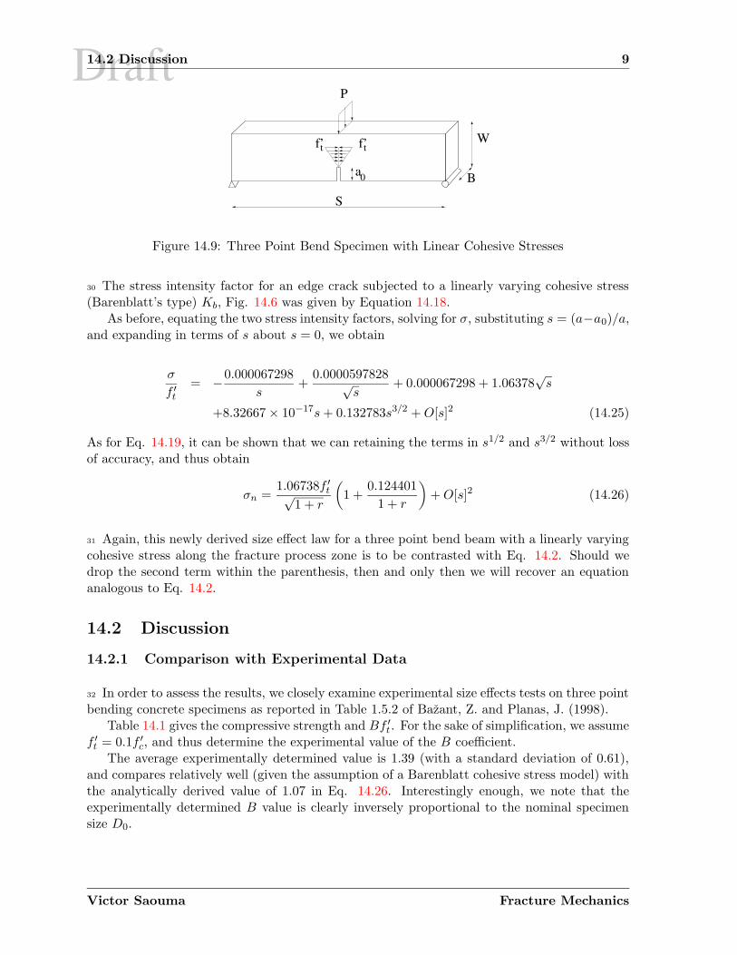
Draft14.2 Discussion 9

S

a

f’t f’t

P

W

0 B

Figure 14.9: Three Point Bend Specimen with Linear Cohesive Stresses

30 The stress intensity factor for an edge crack subjected to a linearly varying cohesive stress(Barenblatt’s type) Kb, Fig. 14.6 was given by Equation 14.18.

As before, equating the two stress intensity factors, solving for σ, substituting s = (a−a0)/a,and expanding in terms of s about s = 0, we obtain

σ

f ′t= −0.000067298

s+

0.0000597828√s

+ 0.000067298 + 1.06378√s

+8.32667 × 10−17s+ 0.132783s3/2 +O[s]2 (14.25)

As for Eq. 14.19, it can be shown that we can retaining the terms in s1/2 and s3/2 without lossof accuracy, and thus obtain

σn =1.06738f ′t√

1 + r

(

1 +0.124401

1 + r

)

+O[s]2 (14.26)

31 Again, this newly derived size effect law for a three point bend beam with a linearly varyingcohesive stress along the fracture process zone is to be contrasted with Eq. 14.2. Should wedrop the second term within the parenthesis, then and only then we will recover an equationanalogous to Eq. 14.2.

14.2 Discussion

14.2.1 Comparison with Experimental Data

32 In order to assess the results, we closely examine experimental size effects tests on three pointbending concrete specimens as reported in Table 1.5.2 of Bazant, Z. and Planas, J. (1998).

Table 14.1 gives the compressive strength and Bf ′t . For the sake of simplification, we assumef ′t = 0.1f ′c, and thus determine the experimental value of the B coefficient.

The average experimentally determined value is 1.39 (with a standard deviation of 0.61),and compares relatively well (given the assumption of a Barenblatt cohesive stress model) withthe analytically derived value of 1.07 in Eq. 14.26. Interestingly enough, we note that theexperimentally determined B value is clearly inversely proportional to the nominal specimensize D0.



strength criterion governs.

3. Again for small structures (small β), B = σN

f ′

tand can be determined from plastic limit

analysis.

4. For structures with very large size compared to aggregate size, λλ0

1. Thus Eq. 14.27

reduces to f∗t ' f ′t√

λ0

λ , and we see that “For very large concrete structures, such as dams

(or large rock masses), Eq. 14.27 asymptotically approaches the size effect of linear elasticfracture mechanics”.

5. In general, Eq. 14.27 represents a gradual transition from the strength criterion for smallstructures to linear elastic fracture mechanics for large structures.

6. To assess the size effect law, geometrically identical specimens, but with different sizesmust be tested. Then Eq. 14.27 can be cast in the form:

Y = a+ bλ =1

σ2N

, (14.28)

where a = 1B2 and b = 1

B2λ0. From statistical regression analysis, the intercept a, and the

slope b can be determined, and then B = 1√a

and λ0 = ab

7. If λλ0

= β is less than 0.1, then a strength criterion must be used, and if β is greater than10, then a LEFM criterion is to be used. Note that those are arbitrary guidelines.

8. The point of intersection of the two asymptotes corresponds to β = 1.

9. At no stage did we have to introduce (explicitly or implicitly) any LEFM equation (inthe sense of a stress singularity at the crack tip).

10. The square root relationship between f ∗t and d (through λ) comes from:

• an appropriate choice of the normalizing parameter for the crack length a in definingα1 and α2.

• expression for GF in terms of the square of f ′t in Eq. ??. Although it is correct todirectly relate GF to the area under the uniaxial stress strain curve (a measure ofthe energy required to produce a unit surface), the square component is again notlinked to LEFM.

11. It can be shown, (Bazant and Cedolin 1991) that the fracture energy GF can be recoveredfrom the Size Effect Law

12. There is a strong analogy between the size effect and column buckling, Fig. 14.11, Table14.2.

14.2.3 LEFM vs NLFM Analyses

36 Ideally, we should extend the analytical solution to encompass Hillerborg’s model as appliedto a three point bending concrete specimen. To the best of the author’s knowledge only tworesearchers addressed this complex nonlinear problem. Xu and Reinhardt (2000) developed aclosed form solution, albeit an empirical one (as termed by its authors). Another solution was



presented by Karihaloo (1999) who again indirectly solved this problem, but with some ratherrestricting assumptions by enforcing a zero net stress intensity factor at the tip of the FPZ.Because of the restrictions imposed to those two solutions, the authors have not consideredthem in this study.

37 In a nonlinear fracture mechanics analysis the crack growth criteria is stress based, i.e thecrack tip maximum tensile stress can not exceed the (non-zero) concrete tensile strength. Al-ternatively, in an LEFM analysis, we can set as a criteria a zero fracture toughness.

38 Whereas both criteria are readily accepted by the research community, practicing engineershave difficulties in accepting a non-zero tensile strength (hence rendering a NLFM analysisimpossible), but can accept a small (preferably zero) fracture toughness, (Federal RegulatoryCommission 1991) (in this context, the double-K method might be more acceptable to practicingengineers than solutions based on GF and a non-zero f ′t). By the same token, a NLFM analysisshould extend the fracture process zone to the point where the stress singularity no longerexists.

39 In order to highlight the duality between a zero fracture toughness criteria in an LEFManalysis, and a non-zero tensile strength criteria in a NLFM analysis a series of numericalanalysis were performed. Considering a three point bend specimen, with GF =100 N/m, f ′t=2MPa, S/W = 8, a/W = 0.6, s0=100 mm, beams with s0, 10s0, 50s0 and 100s0 were analyzedusing the code Merlin (Cervenka, Reich and Saouma 1997–2003). Through those analyses, thetwo stress intensity factors Ka (caused by the external load) and Kb (caused by the cohesiveHillerborg’s stress) were determined. Whereas contour integral techniques should be favored,one should be careful to leave a small zone at the tip of the crack traction free, otherwise theJ integral will be equal to zero. Hence, in the context of this analysis (with surface traction onthe crack faces) we used singular elements.

40 In each analysis, Pmax corresponded to the onset of unstable crack growth (based on tensilestress at the crack tip), and the corresponding stress intensity factor Ka+b were determined. Itshould be noted that in our implementation of the interface element (based on the extendedHillerborg’s model) pre-peak crack opening can occur. This results in a nonlinear pre-peakload-cod curve.

41 Whereas the variation of Pmax with respect to s was indeed according to Bazant’s size effectlaw, the net stress intensity factors at Pmax ranged between 0.05 and 1.5 MPa

√mm. Given

that a representative value for the fracture toughness of concrete is about 1 MPa√

m or 31MPa

√mm, the net stress intensity factor can be considered as essentially zero. These values

should be independent of the tensile strength, as a higher f ′t would result in a larger externalload, and a higher Ka, but also in a higher (negative) Kb caused by the cohesive stresses.Indeed, when the tensile strength was increased from 2 MPa to 4 MPa, Pmax was about twicethe original values, however there was no discernable variation in Ka+b.

42 Thus, we conclude that for all practical purposes a NLFM analysis yields a very small non-zero stress intensity factor in comparison with fracture toughness. Hence, practicing engineerswho accept a zero fracture toughness LEFM analysis should be reassured that a non-zero tensilestrength in the context of a NLFM is, for all practical purposes, identical.


Draft

Chapter 15

FRACTALS, FRACTURES andSIZE EFFECTS

Adapted from (?)

15.1 Introduction

15.1.1 Fracture of Concrete

There is not yet a standard for concrete fracture testing although several have been proposed(RILEM, 1985). Concrete fracture properties include fracture toughness KIc, characteristiclength lch, brittleness number β, fracture energy GF , crack-tip opening displacement CTOD,and at least three additional parameters that characterize the concrete strain softening curve.

This chapter addresses a technique that uses fractal geometry to determine whether there isany surface indication of the direction of crack propagation in concrete and whether there is acorrelation between fracture properties (KIc and GF , which characterize the material resistanceto cracking) and the roughness of the fracture surface as characterized by the fractal dimensionD. The implications of the fractal nature of the cracked surface on the “true” fracture or surfaceenergy are then discussed.

15.1.2 Fractal Geometry

Although most manmade objects have linear or smoothly curvilinear shapes, natural objects(such as rivers, mountains, clouds, and fractures) are commonly rough, fragmented, or dis-continuous. The apparent randomness of these irregularities, coupled with our bias towardEuclidian geometry, handicapped us in studying and properly modeling such objects until theadvent of fractal geometry (Mandelbrot, 1983) .

By definition, an inherent property of fractal objects is the statistical replication of patternsat different scales; a magnified part of a fractal object is statistically identical to the whole.Hence, Fig. 15.1-A illustrates the generation of a self-similar synthetic fractal curve, the triadicKoch curve.. First, an initiator, which represents an initial geometric form, is defined, then agenerator, which describes a transformation on the initiator, is applied. As the transformationoperation is repeatedly applied to the figure, a fractal curve is generated. For the triadic Kochcurve, we note that at each step the number of line segments is increased by a factor of 4 andthat the length of each new line segment generated is one third the length of line segmentsin the previous generation. This increases the total length of the fractal curve by four thirds

Draft16.2 Experiments 3

Table 16.2: Experimentally obtained material properties of the concrete mixes used.

MSA f ′c, MPa (psi) f ′

t,sp, MPa(psi) Eeff , MPa (ksi)

19-mm (0.75-in.) 25.6 (3,710) 2.81 (407) 18,000 (2,610)38-mm (1.5-in.) 24.8 (3,600) 2.67 (388) 16,900 (2,460)

38-mm (1.5-in.) sub-angular 36.6 (5,317) 3.96 (574) 23,200 (3,360)76-mm (3.0-in.) 18.9 (2,740) 2.41 (349) 16,500 (2,400)

Figure 16.1: *Wedge-splitting specimen geometry.

of small concrete specimens (Hillemeier & Hilsdorf 1976, Linsbauer & Tschegg 1986, Bruhwiler1988, Bruhwiler & Wittmann 1990). The WS specimen has a large fracture area compared tothe concrete volume, approximately 4.6 times greater than a commonly used three-point bend(TPB) beam geometry (RILEM 1985) of equal volume. The large fracture area compared tothe aggregate size and specimen volume makes the WS geometry well suited for testing largeMSA and specimens under laboratory conditions.

The dimensions of the WS specimens tested in the experimental program are summarized inTable 16.3. The specimen dimensions and aggregate sizes were selected to enable a comparison

Table 16.3: Wedge-splitting specimen dimensions.

Specimen Dimensions, cm (in.)

Specimen Type H w t s D a0 h

“Small” 31 (12.0) 31 (12.0) 23 (9.0) 6 (2.25) 3 (1.0) 4.5(1.75) 20 (8.0)“Medium” 91 (36.0) 91 (36.0) 41 (16.0) 15 (6.0) 8 (3) 15.2 (6.0) 61 (24.0)“Large” 152 (60.0) 152 (60.0) 41 (16.0) 15 (6.0) 8 (3) 30.5 (12.0) 107 (42.0)

with results previously obtained by other researchers in the academic community, and to predictfracture properties of dam concrete with intermediary values to ensure a continuity of results.

Specimen construction consisted of wooden formwork built for the placing of the concrete, asharpened 3.2-mm (0.125-in.) thick steel plate mounted inside each form to obtain the verticalnotch normal to the load line, and two hollow steel sleeves flanking the plate. Two differentready–mix suppliers delivered the concrete. The first provided the 19-mm and 38-mm MSAmixes and the other the 76-mm MSA concrete mix. In all specimens, with the exception of thecold-joint (CJ) specimens, the concrete was placed with the notch in the vertical direction, andcured at room temperature in the laboratory for at least 28 days prior to testing.

For the CJ specimens, the concrete was placed in two separate lifts, with the notch plateinitially in a horizontal orientation. The tendency of the crack to propagate into the cold-joint,which is a region of inherent weakness, was studied through a slight offset between the initialnotch and the level of the concrete in the first lift. Three days after the first lift was placed, the


Draft16.2 Experiments 5

16.2.3 Testing Procedure

The experimental setup of the electronic controller, the data acquisition system, and the testingmachine for the WS specimen tests are shown in a simplified block diagram in Fig. 16.3. In the

Figure 16.3: *Block diagram of the experimental system.

WS specimen experiments, the primary deformation monitored was the crack–mouth openingdisplacement (CMOD). The CMOD was measured on the top surface of the specimen by a clipgage mounted over the mouth of the initial notch. The closed-loop servo-hydraulic test machineused a programmed constant rate of CMOD (1.0-µm/sec, or 40-µin/sec) as the feedback controlto obtain stable crack growth with structural post-peak response. During the test, the verticalload and the CMOD were monitored and recorded using a standard data acquisition system.Unload/reload cycles, which were used to monitor the change in the specimen compliance, orflexibility, were performed. The experiment was performed until the specimen was split intotwo halves.

The vertical force induced by the wedge fixture, PV , was directly obtained from the load cellof the testing machine. The wedge fixture is a statically determinate beam, and therefore, thesplitting force is given by PSP = PV

2·tanα , where the wedge angle, α, is equal to 15o. (Frictionalforces were neglected; they were reduced by using hardened steel inserts along the inclinedwedge surface and needle bearings with a low coefficient of friction.) A typical PSP vs. CMODcurve representative of the WS specimens is presented in Fig. 16.4. In the PSP vs. CMOD

Figure 16.4: *Typical PSP vs. CMOD curve for a “Large” specimen.

curve, both linear and nonlinear responses in the ascending prepeak branch and a descendingpostpeak branch can be observed.

16.2.4 Acoustic Emissions Monitoring

In several WS tests, the microcracking associated with fracture process zone (FPZ) formationand with transient releases of elastic energy due to localized aggregate fracture and bond failurewere monitored with an acoustic emission (AE) sensor mounted on the surface of the specimen.Inside the sensor, a piezoelectric crystal is stimulated by the stress waves and produces electricalsignals. The signals are then amplified, filtered, processed, and related to the behavior of thematerial throughout the experiment.

The AE sensor was mounted on the face of the specimen in a direction such that the sensorwas normal to the predicted fracture plane. The sensor used during testing was sensitive in


Draft

Chapter 17

SINGULAR ELEMENT

17.1 Introduction

1 For most practical problems, either there is no analytical solution, or the handbook ((Tadaet al. 1973)) ones are only crude approximation. Hence numerical techniques should be used.Whereas Boundary Element Methods are increasingly being used, (Aliabadi and Rooke 1991),they are far behind in sophistication the Finite Element Methods which will be exclusivelycovered in this chapter. For an overview of early finite element techniques in finite elements thereader should consult (Owen and Fawkes 1983), some of the more recent methods are partiallycovered in (Anderson 1995). Finally, the Ph.D. thesis of Reich (1993) and of ? contain someof the major extensions of modern techniques to include thermal load, body forces, surfacetractions in 2D and 3D respectively.

2 Numerical methods for fracture mechanics can be categorized in many different ways, in thischapter we shall use three criteria:

1. Those in which the singularity is modelled, that is the r−12 stress field at the tip of the

crack is properly represented.

2. Techniques in which the SIF are directly evaluated as part of the augmented global stiffnessmatrix.

3. Techniques through which the SIF can be computed a post priori following a standardfinite element analysis via a special purpose post-processor.

17.2 Displacement Extrapolation

3 This technique was the predominant one prior to the serendipitous discovery of the quarterpoint singular element.

4 In early finite element studies of LEFM, it was recognized that unless singular elements couldbe used, it would necessitate to have a very fine mesh at the crack tip to approximate the stresssingularity with non-singular elements.

5 Following a liner elastic analysis, the stress intensity factors were determined by equating thenumerically obtained displacements with their analytical expression in terms of the SIF. Such

Draft17.4 Review of Isoparametric Finite Elements 3

1. cover a brief review of the isoparametric element formulation

2. show how the element can be distorted in order to achieve a stress singularity

3. determine the order of the stress singularity

4. provide a brief review of all the historical developments surrounding this element

5. discuss the effect on numerical accuracy of element size, order of integration, and localmeshing around the crack tip

6. briefly mention references to other singular elements

17.4 Review of Isoparametric Finite Elements

12 In the isoparametric finite element representation, both the internal displacement and coor-dinates are related to their nodal values through the shape functions:

1 2

34

5

6

7

8

1 2

34

5

6

7

8

x,u

y,v

ξ

η

1

1

1 1

Figure 17.2: Isoparametric Quadratic Finite Element: Global and Parent Element

xy

=8∑

i=1

[

Ni 00 Ni

]

xi

yi

(17.2)

d =

uv

=8∑

i=1

[

Ni 00 Ni

]

ui

vi

(17.3)

where the Ni are the assumed shape functions.

13 The shape functions are obtained by mere inspection (i.e. serependitiously),

Ni = 14 (1 + ξξi) (1 + ηηi) (ξξi + ηηi − 1) i = 1, 2, 3, 4

Ni = 12

(1 − ξ2

)(1 + ηηi) i = 5, 7

Ni = 12 (1 + ξξi)

(1 + η2

)i = 6, 8

(17.4)

and are tabulated in Table 17.1.


Draft

Chapter 18

ENERGY RELEASE BASEDMETHODS

1 In this class of solutions, we will exploit the definition of the energy release rate G to derive asimple method of determining the stress intensity factors. We shall distinguish between modeI and mixed mode cases. The former one, although of academic relevance only, is a simpleintroduction to the second.

18.1 Mode I Only

18.1.1 Energy Release Rate

2 Recalling that the strain energy release rate G is given by:

G = −∂U∂a

=K2

I

E′ ' ∆U

∆a(18.1)

a simple algorithm for the SIF calculation emerges:

1. For an initial crack length a, determine the total strain energy from either one of thefollowing approaches:

(a) U = utKu where u is nodal displacement, and K is the global structural stiffnessmatrix.

(b) U = utP where P and u are the externally applied nodal load and displacement,respectively.

2. Increase the crack length from a to a+ ∆a, Fig. 18.1, and reanalyze.

3. Determine G from G ' (U+∆U)−U(a+∆a)−a = ∆U

∆a =K2

I

E′

3 Note that:

1. This procedure requires two complete separate analyses.

Draft

Chapter 19

J INTEGRAL BASED METHODS

19.1 Numerical Evaluation

1 Within linear elastic fracture mechanics, the J integral is equivalent to G and we have:

G = J = −∂Π

∂a=

∫

r(wdy − t · ∂d

∂xds) (19.1)

2 Thus it is evident that we do have two methods of evaluating J : the first one stems from itsequivalence to the energy released rate, and the second one from its definition as an integralalong a closed contour. Evaluation of J according to the first approach is identical to the oneof G and has been previously presented.

3 In this chapter we shall present the algorithm to evaluate J on the basis of its contour lineintegral definition. Whereas derivation will be for J integral only, its extension to Ji is quitestraightforward.

4 If the stresses were to be determined at the nodes, than the numerical evaluation of J willbe relatively simple. However, most standard finite element codes only provide Gauss pointstresses, and hence care must be exercised in properly determining the J integral along a pathpassing through them.

5 The algorithm for the J calculation closely follows the method presented in (Owen and Fawkes1983), and is as follows:

1. First let us restrict ourselves to the more general case in which isoparametric elementsare used. Because the stresses are most accurately evaluated at the gauss points, thepath can be conveniently chosen to coincide with ξ = ξcst and/or η = ηcst. For the sakeof discussion, let us assume that the element connectivity is such that the path is alongξ = ξcst, as in Fig. 19.1. We note that for corner elements the integration will have to beperformed twice along the two directions.

2. Now let us start from the basic definition of J :

J =

∫

Γwdy − t · ∂d

∂xds (19.2)

where t is the traction vector along n, which is normal to the path; d is the displacementvector; ds is the element of arc along path Γ; and w is the strain energy density. We note

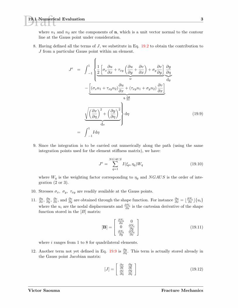
Draft19.1 Numerical Evaluation 3

where n1 and n2 are the components of n, which is a unit vector normal to the contourline at the Gauss point under consideration.

8. Having defined all the terms of J , we substitute in Eq. 19.2 to obtain the contribution toJ from a particular Gauss point within an element.

Je =

∫ 1

−1

1

2

[

σx∂u

∂x+ τxy

(∂u

∂y+∂v

∂x

)

+ σy∂v

∂y

]

︸︷︷︸

w

∂y

∂η︸︷︷︸

dy

−[

(σxn1 + τxyn2)∂u

∂x+ (τxyn1 + σyn2)

∂v

∂x

]

︸︷︷︸

t· ∂d

∂x

√(∂x

∂η

)2

+

(∂y

∂η

)2

︸︷︷︸

ds

dη (19.9)

=

∫ 1

−1Idη

9. Since the integration is to be carried out numerically along the path (using the sameintegration points used for the element stiffness matrix), we have:

Je =NGAUS∑

q=1

I(ξp, ηq)Wq (19.10)

where Wq is the weighting factor corresponding to ηq and NGAUS is the order of inte-gration (2 or 3).

10. Stresses σx, σy, τxy are readily available at the Gauss points.

11. ∂u∂x , ∂u

∂y , ∂v∂x , and ∂v

∂y are obtained through the shape function. For instance ∂u∂x = b∂Ni

∂x cuiwhere the ui are the nodal displacements and ∂Ni

∂x is the cartesian derivative of the shapefunction stored in the [B] matrix:

[B] =

∂Ni

∂x 0

0 ∂Ni

∂y∂Ni

∂y∂Ni

∂x

(19.11)

where i ranges from 1 to 8 for quadrilateral elements.

12. Another term not yet defined in Eq. 19.9 is ∂y∂η . This term is actually stored already in

the Gauss point Jacobian matrix:

[J ] =

[∂x∂ξ

∂y∂ξ

∂x∂η

∂y∂η

]

(19.12)


Draft

Chapter 20

RECIPROCAL WORKINTEGRALS

Chapter adapted from (Reich 1993)

20.1 General Formulation

1 In addition to conservation laws, a form of Betti’s reciprocal work theorem (Sokolnikoff 1956)can also be exploited to directly compute stress intensity factors (Stern 1973). The reciprocalwork theorem defines the relationship between two equilibrium states for a solid.

2 For a solid free of body forces and initial strains and stresses the reciprocal work theorem isdefined as

∮

Γti ui dΓ =

∮

Γti ui dΓ (20.1)

where Ω is any simply connected region within the solid and Γ is the contour of that region; ui

and ti are the displacements and surface tractions, respectively, associated with one equilibriumstate and ui; and ti are the displacements and surface tractions, respectively, associated withanother equilibrium state.

3 The equilibrium state defined by ui and ti is called the primary state and the equilibriumstate defined by ui and ti is called the complementary or auxiliary state.

4 To apply the reciprocal work theorem to a cracked solid the simply connected region Ω mustbe defined such that the singularity at the crack tip is avoided. This is accomplished by defininga pair of surfaces, Γ and Γε, that begin on one crack surface and end on the other.

5 Γ is an arbitrary surface defined in the counter-clockwise direction around the crack tip butfar away from it.

6 Γε is a circle of radius ε centered on the crack tip that is defined in the clockwise directionaround the crack tip completely inside Γ.

7 Another pair of surfaces, Γ+t and Γ−

t , corresponding to the crack surfaces complete the defi-nition of Γ, as is shown in Figure 20.1. Γ+

t is defined on the upper crack surface between Γ andΓε and Γ−

t is defined on the lower crack surface bewteen Γε and Γ.

Draft

Chapter 21

FICTITIOUS CRACK MODEL

Originally published as:

Implementation and Validation of a nonlinear fracture model in a 2D/3D finite elementcode by Reich, Plizzari, Cervenka and Saouma; in Numerical Models in Fracture of Concrete;Wittman Ed., Balkema (1993).

1 An incremental formulation for the Fictitious Crack Model (FCM) will be presented. Thecomputational algorithm treats the structure as a set of sub-domains bonded along assumedcrack paths. The crack paths are defined by interface elements that initially act as constraintsenforcing the bond between adjacent sub-domains, but change state to function as standardinterface elements as the crack propagates. Constraints are enforced on the global system ofequations using a penalty approach.

2 A load scaling strategy, which allows for load controlled analyses in the post-peak regime, isused to enforce stress continuity at the tip of the Fracture Process Zone (FPZ).

3 To demonstrate the accuracy of the computational algorithm, a series of three wedge-splitting(WS) test specimens are analyzed. Specimen sizes are 31, 91, and 152 cm (1, 3, and 5 ft).Material properties for the concrete are taken as the mean values of the observed experimentalresults for all specimen sizes. The computed results are compared to the envelopes of theexperimental response for each specimen size.

21.1 Introduction

4 The most commonly implemented nonlinear fracture model for concrete using the discretecrack approach is the FCM (Hillerborg, A. and Modeer, M. and Petersson, P.E. 1976). Inthe FCM the zone of micro-cracking and debonding ahead of the crack front is modeled as acohesive stress that acts to close the crack. The magnitude of the cohesive stresses on the cracksurface are determined by a softening law that relates the stress to the relative displacement ofthe crack surfaces through the fracture energy.

5 Many implementations of the FCM have been reported (Ingraffea and Gerstle 1984, Roelfstraand Sadouki 1986, Dahlblom and Ottosen 1990, Bocca, Carpinteri and Valente 1990, Gopalarat-nam and Ye 1991, Gerstle and Xie 1992), but none of the implementations based on a discrete

Draft21.2 Computational Algorithm 3

Ω

Ω

Γ

Γ

Γ

Γ

Γ

Γt

u

t

u

I

I

1

2

t

t

b

c

1

1

2

2

2

1

Figure 21.1: Body Consisting of Two Sub-domains

10 Defining the interface surface asΓI = ΓIb

∪ ΓIc , (21.6)

where ΓIbis the bonded interface surface and ΓIc is the interface surface subject to cohesive

stresses, the external work on the interface is written as∫

ΓI

δuT1 tI1dΓ =

∫

ΓIb

δuT1 tbdΓ +

∫

ΓIc

δuT1 tcdΓ (21.7-a)

∫

ΓI

δuT2 tI2dΓ = −

∫

ΓIb

δuT2 tbdΓ −

∫

ΓIc

δuT2 tcdΓ (21.7-b)

Both tb and tc are unknown, but as tb acts on the bonded, or constrained, interface it will betreated as a Lagrange multiplier

λ = tb (21.8)

11 Substituting λ into Equations 21.3 and 21.4-a-21.4-c and including the external work per-formed by the surface tractions on the interface surface, the Principle of Virtual Work forsub-domains Ω1 and Ω2 is written as

∫

Ω1

δεT1 σ1dΩ −

∫

Ω1

δuT1 b1dΩ −

∫

Γt1

δuT1 t1dΓ −

∫

ΓIb

δuT1 λdΓ −

∫

ΓIc

δuT1 tcdΓ = 0

∫

Ω2

δεT2 σ2dΩ −

∫

Ω2

δuT2 b2dΩ −

∫

Γt2

δuT2 t2dΓ +

∫

ΓIb

δuT2 λdΓ +

∫

ΓIc

δuT2 tcdΓ = 0

(21.9)

12 On ΓIbthe displacements for the two sub-domains, u1 |ΓIb

and u2 |ΓIb, must be equal. This

condition can be written as a constraint in the strong form

u2 |ΓIb−u1 |ΓIb

= 0, (21.10)


Draft

Chapter 22

INTERFACE CRACK MODEL

This chapter was chapter 6 of the PhD thesis of Cervenka

1 This chapter discusses the nonlinear modeling of concrete using a discrete crack fracture me-chanics based model. It addresses two important issues: mixed mode fracture in homogeneousmaterials and interface fracture. A new three-dimensional interface crack model is derived. Themodel is a generalization of classical Hillerborg’s fictitious crack model, which can be recoveredif shear displacements are set to zero. Several examples are used to validate the applicabilityof the proposed interface crack model. First, direct shear tests on mortar joints are used totest the model performance in the shear-compression regime. The more complicated combina-tion of shear-tension is investigated using large biaxial tests of concrete-rock interfaces. Theapplicability to mixed mode cracking in homogeneous concrete is tested using experiments onmodified Iosipescu’s shear beam and anchor bolt pull-out tests.

22.1 Introduction

2 The assumption of singular stresses at the crack tip is mathematically correct only within theframework of linear elastic fracture mechanics, but physically unrealistic.

3 In concrete materials, a fracture process zone (Section ??) exists ahead of the crack tip.The most popular model simulating this behavior is Hillerborg’s fictitious crack model (FCM)described in Section ?? and Figure ??. In a previous work, the classical FCM model wasimplemented by (Reich 1993) for mode I crack propagation, and extended to account for theinfluence of water pressure inside the crack.

4 The classical FCM model, Chapter 21, defines a relationship between normal crack openingand normal cohesive stresses, and assumes that there are no sliding displacements nor shearstresses along the process zone. This assumption is only partially valid for concrete materials.Based on experimental observations, it is indeed correct that a crack is usually initiated in puremode I (i.e. opening mode) in concrete, even for mixed mode loading. However, during crackpropagation, the crack may curve due to stress redistribution or non-proportional loading, andsignificant sliding displacements develop along the crack as schematically shown in Figure 22.1.Therefore, it is desirable to incorporate these shear effects into the proposed crack model.

5 Finally for concrete dams, it is well accepted that the weakest part of the structure is thedam-foundation interface, which is also the location of highest tensile stresses and lowest tensile

Draft22.2 Interface Crack Model 3

0.0 0.5 1.0 1.5 2.0CMOD [mm]

0.0

0.5

1.0

1.5

2.0

2.5

Ver

tical

Loa

d [k

N]

12

3

1. Solid Concrete GF = 158.9 N/m

2. Solid Limestone GF = 41.8 N/m

3. Limestone-Concrete GF = 39.7 N/m

Figure 22.2: Wedge splitting tests for different materials, (Saouma V.E., and Cervenka, J. andSlowik, V. and Chandra Kishen, J.M. 1994)

is not abrupt, but is rather gradual. This is caused by the presence of the fracture process zone,along which the energy of the system is gradually dissipated.

12 In the present model, the rock-concrete contact is idealized as an interface between twodissimilar materials with zero thickness. Thus, the objective is to define relationships betweennormal and tangential stresses with opening and sliding displacements. The notation used inthe interface model is illustrated in Figure 22.2.

13 The major premises upon which the model is developed are:(1) Shear strength depends on the normal stress.(2) Softening is present both in shear and tension.(3) There is a residual shear strength due to the friction along the interface, which depends

on the compressive normal stress.(4) Reduction in strength, i.e. softening, is caused by crack formation.(5) There is a zero normal and shear stiffness when the interface is totally destroyed.(6) Under compressive normal stresses neither the shear and nor the normal stiffnesses

decrease to zero. In addition, should a compressive stress be introduced in the normal directionfollowing a full crack opening, two faces of the interface come to contact, and both tangentialand normal stiffnesses become nonzero.

(7) Irreversible relative displacements are caused by broken segments of the interface mate-rial and by friction between the two crack surfaces.

(8) Roughness of the interface causes opening displacements (i.e. dilatancy) when subjectedto sliding displacements.

(9) The dilatancy vanishes with increasing sliding or opening displacements.

14 Figure 22.4 illustrates the probable character of the fracturing process along an interface.

15 In the proposed model the strength of an interface is described by a failure function:

F = (τ21 + τ2

2 ) − 2 c tan(φf )(σt − σ) − tan2(φf )(σ2 − σ2t ) = 0 (22.1)


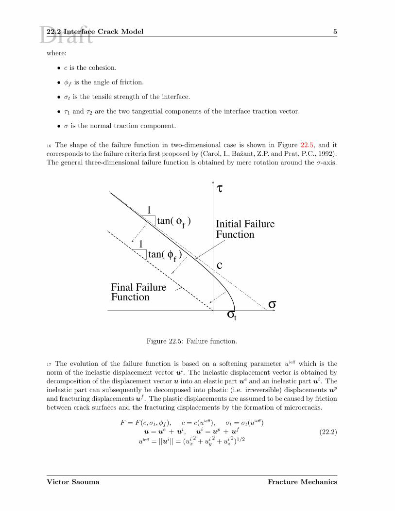
Draft22.2 Interface Crack Model 5

where:

• c is the cohesion.

• φf is the angle of friction.

• σt is the tensile strength of the interface.

• τ1 and τ2 are the two tangential components of the interface traction vector.

• σ is the normal traction component.

16 The shape of the failure function in two-dimensional case is shown in Figure 22.5, and itcorresponds to the failure criteria first proposed by (Carol, I., Bazant, Z.P. and Prat, P.C., 1992).The general three-dimensional failure function is obtained by mere rotation around the σ-axis.

φ

tan( )φf

Final FailureFunction

Initial FailureFunction

σ

τ

c

σ

tan( )f

t

1

1

Figure 22.5: Failure function.

17 The evolution of the failure function is based on a softening parameter uieff which is thenorm of the inelastic displacement vector u

i. The inelastic displacement vector is obtained bydecomposition of the displacement vector u into an elastic part u

e and an inelastic part ui. The

inelastic part can subsequently be decomposed into plastic (i.e. irreversible) displacements up

and fracturing displacements uf . The plastic displacements are assumed to be caused by friction

between crack surfaces and the fracturing displacements by the formation of microcracks.

F = F (c, σt, φf ), c = c(uieff), σt = σt(uieff)

u = ue + u

i, ui = u

p + uf

uieff = ||ui|| = (uix2+ ui

y2+ ui

z2)1/2

(22.2)


Draft

Bibliography

399, A.: n.d., Standard Test Method for Plane Strain Fracture Toughness of Metallic Materials,E399–74, Annual Book of ASTM Standards.

446, A. C.: 1991, Fracture mechanics of concrete: Concepts, models and deformation of materialproperties, Technical Report ACI 446.1R-91, American Concrete Institute, Detroit, MI.

Abramowitz, M. and Stegun, I.: 1970, Handbook of mathematical functions, Technical report,National Bureau of Standard. Applied Mathematics Series, No. 55.

Advani, S. and Lee, K.: 1979, Thermo-mechanical failure criteria for rock media, pp. 19–25.

Aliabadi, M. and Rooke, D.: 1991, Numerical Fracture Mechanics, Kluwer Academic Publishers.

Alvaredo, A. and Wittman, F.: 1992, Crack formation due to hygral gradients, Third Interna-tional Workshop on Behaviour of Concrete Elements Under Thermal and Hygral Gradients,Weimar, Germany.

Anderson, T.: 1995, Fracture Mechanics, Fundamentals and Applications, CRC Press.

Anon.: 1985, RILEM Draft Recommendation (50–FCM): Determination of the Fracture Energyof Mortar and Concrete by Means of Three–Point Bend Tests on Notched Beams, Materialsand Structures 18, 287–290.

Apostal, M.: 1974, Development of an Anisotropic Singularity Finite Element Utilizing theHybrid Displacement Method, PhD thesis, State University of New York.

Atkinson, C. and Bastero, J.: 1991, On the use of betti’s reciprocal theorem for computing thecoefficients of stress singularities in anisotropic media, International Journal of EngineeringScience 29(6), 727–741.

Atkinson, C., Bastero, J. and Martinez-Esnaola, J.: 1988, Stress analysis in sharp angularnotches using auxiliary fields, Engineering Fracture Mechanics 31(4), 637–646.

Atkinson, C., Bastero, J. and Miranda, I.: 1986, Path-independent integrals in fracture dynam-ics using auxiliary fields, Engineering Fracture Mechanics 25(1), 53–62.

Atkinson, C. and Craster, R.: 1992, The application of invariant integrals in diffusive elasticsolids, Philosophical Transactions of the Royal Society of London, Series A 399(1653), 231–263.

Atluri, S.: 1982, Path-independent integrals in finite elasticity and inelasticity, with body forces,inertia, and arbitrary crack-face conditions, Engineering Fracture Mechanics 16(3), 341–364.

DraftBIBLIOGRAPHY 3

Bazant, Z.: 1985, Comment on hillerborg’s comparison of size effect law with fictitious crackmodel, in ’Dei Poli Anniversary Volume’ edited by L. Cedolin, Politecnico di Milanopp. 335–338.

Bazant, Z. and Cedolin, L.: 1991, Stability of Structures, Oxford University Press.

Bazant, Z. (ed.): 1992, Proceedings of the First International Conference on Fracture Mechanicsfor Concrete and Concrete Structures, Elsevier, Breckenridge, CO.

Bazant, Z. and Pfeiffer, P.: 1987, Determination of fracture energy properties from size effectand brittleness number, ACI Material Journal 84(6), 463–480.

Bazant, Z. and Planas, J.: 1998, Fracture and Size Effect in Concrete and Other QuasibrittleMaterials, CRC Press.

Bazant, Z.P.: 1984, Size effect in blunt fracture: Concrete, rock, metal, J. of EngineeringMechanics, ASCE 110(4), 518–535.

Bazant, Z.P. and Cedolin, L.: 1979, Blunt crack propagation in finite element analysis, J. ofthe Engineering Mechanics Division, ASCE 105, 297–315.

Benzley, S.: 1974, Representation of singularities with isoparametric finite elements, Int. J.Num. Meth. Engng. 8, 537.

Bocca, P., Carpinteri, A. and Valente, S.: 1990, Size effects in the mixed mode crack propaga-tion: Softening and snap-back analysis, Engineering Fracture Mechanics 35(1–3), 159–170.

Bouchaud, E., Lapasset, G. and Planes, J.: 1990, Fractal dimension of fractured surfaces: auniversal value?, Europhysics Letters 13(1), 73–79.

Bourdarot, E., Mazars, J. and Saouma, V. (eds): 1994, Proceedings of the International Work-shop on Dam Fracture and Damage, Balkema.

British Standards Institution, BS 5447, London: 1977.

Broek, D.: 1986, Elementary Engineering Fracture Mechanics, 4th Edition, Martinus NijhoffPublishers.

Broek, D.: 1989, The Practical Use of Fracture Mechanics, Kluwer Academic Publishers.

Brown, S.: 1987, A note on the description of surface roughness using fractal dimension, Geo-physical Research Letters 14(11), 1095–1098.

Brown, S.: 1988, Correction to: A note on the description of surface roughness using fractaldimension, Geophysical Research Letters 15(11), 286.

Bruhwiler, E.,: 1988, Fracture Mechanics of Dam Concrete Subjected to Quasi-Static and Seis-mic Loading Conditions, Doctoral Thesis No 739, Swiss Federal Institute of Technology,Lausanne. (in German).

Bruhwiler, E., Broz, J.J., and Saouma, V.E.,: 1991, Fracture model evaluation of dam concrete,ASCE, Journal of Civil Engineering Materials 4, 235–251.


DraftBIBLIOGRAPHY 5

deLorenzi, H.G.: 1985, Energy release rate calculations by the finite element method, Engi-neering Fracture Mechanics 21, 103–110.

Duda, H.: 1990, Stress-crack-opening relation and size effect in high-strength concrete, Dar-mastad Concrete 5, 35–46.

Duga, J., Fisher, W., Buxbam, R., Rosenfield, A., Buhr, A., Honton, E. and McMillan, S.:1983, The economic effects of fracture in the united states, Technical Report SP647-2,National Bureau of Standards.

Dugdale, D.: 1960, Yielding of steel sheets containing slits, J. Mech. Phys. Sol. 8, 100–108.

Dunders, J.: 1969, Edge - bonded dissimilar orthogonal elastic wedges under normal and shearloading, Journal of Applied Mechanics 36, 650–652.

Erdogan, F. and Sih, G.C.: 1963, On the crack extension in plates under plane loading andtransverse shear, Journal of Basic Engineering 85, 519–527.

Eshelby, J.: 1974, Calculation of energy release rate, Prospect of Fracture Mechanics Nordhoffpp. 69–84.

Fawkes, A., Owen, D. and Luxmoore, A.: 1979, An assessment of crack tip singularity modelsfor use with isoparametric elements, Eng. Fract. Mech. 11, 143–159.

Feder, J.: 1988, Fractals, Plenum Press.

Federal Regulatory Commission: 1991, Engineering guidelines for the evaluation of hydropowerprojects, Technical report, Federal Energy Regulatory Commission, Office of HydropowerLicensing.

Feenstra P.H., d. B. R. and J., R.: 1991, Numerical study on crack dilatancy. i: Models andstability analysis. ii: Applications, J. Eng. Mech. 117(4), 733–769.

Foreman, R., Kearney, V. and Engle, R.: 1967, Numerical analysis of crack propagation incyclic-loaded structures, J. of Basic Engineering 89, 459–464.

Freese, C. and Tracy, D.: 1976, The natural isoparametric triangle versus collapsed quadrilateralfor elastic crack analysis, Int. J. Fract. 12, 768–770.

Gallagher, R.: 1975, Finite Element Analysis Fundamentals, Prentice Hall, Englewood Cliffs,N.J.

Gdoutos, E.: 1993, Fracture Mechanics; An Introduction, Kluwer Academic Press.

Gerstle, W. and Xie, M.: 1992, Fem modeling of fictitious propagation in concrete, Journal ofEngineering Mechanics 118(2), 416–434.

Giuriani, E. and Rosati, G. P.: 1986, Behaviour of concrete elements under tension after crack-ing, Studi e Ricerche, Corso di Perfezionamento per le Costruzioni in Cemento Armato8, 65–82. (in Italian).

Goodman, R.E., Taylor, R.C. and Brekke, T.C.,: 1968, A Model for the Mechanics of JointedRocks, J. Soil Mech. Div., ASCE 94.


DraftBIBLIOGRAPHY 7

Hudson, C. and Seward, S.: 1978, A Compendium of Sources of Fracture Toughness and FatigueCrack Growth Data for Metallic alloys, Vol. 14, Int. J. of Fracture.

Hudson, C. and Seward, S.: 1982, A compendium of sources of fracture toughness and fatiguecrack growth data for metallic alloys, Int. J. of Fracture, Part II 20, R59–R117.

Hussain, M., Pu, S. and Underwood, J.: 1974, Strain energy release rate for a crack undercombined mode i and mode ii, ASTM, STP 560 pp. 2–28.

Hussain, M., Vasilakis, J. and Pu, L.: 1981, Quadratic and cubic transition elements, Int. J.Num. Meth. Engng. 16, 1397–1406.

Hutchinson, J.: 1968, Singular behavior at the end of a tensile crack tip in a power-law hardeningmaterial, Journal of Mechanics and Physics of Solids 16, 13–31.

Hutchinson, J. W. and Suo, Z.: 1992, Mixed mode cracking in layered materials, Advances inApplied Mechanics 29, 63–191.

Il’yushin, A.: 1946, The theory of small elastic-plastic deformations, Prikadnaia Matematika iMekhanika, PMM 10, 347–356.

Inglis, C.: 1913, Stresses in a plate due to the presence of cracks and sharp corners, Trans. Inst.Naval Architects 55, 219–241.

Ingraffea, A.: 1977, Discrete Fracture Propagation in Rocks: Laboratory Tests and Finite Ele-ment Analysis, PhD thesis, University of Colorado.

Ingraffea, A. and Gerstle, W.: 1984, Non-linear fracture models for discrete crack propagation,in S. Shah (ed.), Proceedings of the NATO Advanced Workshop on Application of FractureMechanics to Cementitious Composites, Martinus Nijhoff, Hingham, Mass, pp. 171–209.

Ingraffea, A. and Manu, C.: 1980, Stress intensity factor computation in three dimension withquarter-point elements, Int. J. num. Meth. Engng. 15(10), 1427–1445.

International Conference on Fracture and Damage of Concrete and Rock: 1988, Vienna. To bePublished in Engineering Fracture Mechanics.

Irwin, G.: 1957, Analysis of stresses and strains near the end of a crack traversing a plate,Transactions ASME, J. Appl. Mech. 24.

Irwin, G.: 1960, Plastic zone near a crack and fracture toughness, Proc. 7th Sagamore Conf.,p. 63.

Irwin, G.: 1962, The crack extension force for a part through crack in a plate, TransactionsASME, J. Appl. Mech. 29.

Ishikawa, H.: 1980, A finite element analysis of stress intensity factors for combined tensile andshear loading by only a virtual crack extension, Int. J. Fracture 16.

Issa, M., Hammad, A. and Chudnovsky, A.: 1993, Correlation between crack tortuosity andfracture toughness in cementitious materials, International Journal of Fracture 60, 97–105.

Jeang, F. L. and Hawkins, N. M.: 1985, Nonlinear analysis of concrete fracture, Structures andmechanics report, Department of Civil Engineering, University of Washington, Seattle,WA.


DraftBIBLIOGRAPHY 9

Lotfi, H.: 1992, Finite Element Analysis of Fracture of Concrete and Masonry Structures, PhDthesis, University of Colorado, Boulder.

Lynn, P. and Ingraffea, A.: 1977, Transition elements to be used with quarter-point crack-tipelements, Int. J. num. Meth. Engng. 11, 1031–1036.

Malyshew, B. M. and Salganik, R. L.: 1965, The strength of adhesive joints using the theoryof cracks, Int. Journal of Fracture 1, 114–118.

Mandelbrot, B.: 1983, The Fractal Geometry of Nature, W.H. Freeman, San Francisco.

Mandelbrot, B., Passoja, D. and Paullay, A.: 1984, Fractal character of fracture surfaces ofmetals, Nature 308, 721–722.

Mecholsky, J. and Freiman, S.: 1991, Relationship between fractal geometry and fractography,Journal of the American Ceramic Society 74(12), 3136–3138.

Mecholsky, J. and Mackin, T.: 1988, Fractal analysis of fracture in ocala chert, Journal ofMaterials Science Letters 7, 1145–1147.

Mecholsky, J., Passoja, D. and Feinberg-Ringle, K.: 1989, Quantitative analysis of brittlefracture surfaces using fractal geometry, Jour. Amer. Ceram. Soc. 72(1), 60–65.

Miller, M. and Gallagher, J.: 1981, An analysis of several fatigue crack growth rate (fcgr)descriptions, in S. Hudak Jr. and R. Bucci (eds), Fatigue Crack Growth Measurements andData Analysis, ASTM STP 738, ASTM, Philadelphia, pp. 205–251.

Mindess, S. and Young, F.: 1981, Concrete, Prentice-Hall, Inc.

Maløy, K., Hansen, A., Hinrichsen, E. and Roux, S.: 1992, Experimental measurements of theroughness of brittle cracks, Physical Review Letters 68(2), 213–215.

Mosolov, A.: 1991, Fractal j integral in fracture, Soviet Technical Physics Letters 17(10), 698–700.

Mostovoy, e. a.: 1967, Use of crack-line loaded specimens for measuring plane strain fracturetoughness, J. of Materials 2(3), 661–681.

Murakami, Y.: 1987, Stress Intensity Factors Handbook, Pergamon Press. (2 Vols).

Newman, J.: 1971, An improved method of collocation for the stress analysis of cracked plateswith various shaped boundaries, Technical Report NASA TN D-6376, National Aeronauticsand Space Administration, Langley Research Center, Hampton, VA.

Newman, J. and Raju, I.: 1981, An emperical stress intensity factor equation for surface cracks,Engineering Fracture Mechanics 15, 185–192.

Newton, R.: 1973, Degeneration of brick-type isoparametric elements, Int. J. num. Meth. En-gng. 7, 579–581.

Nikishkov, G. P. and Atluri, S. N.: 1987, Calculation of fracture mechanics parameters for an ar-bitrary three-dimensional crack, by the ‘equivalent domain integral’ method, InternationalJournal of Numerical Methods in Engineering 24(9), 1801–1821.


DraftBIBLIOGRAPHY 11

Saouma, V., Broz, J., Bruhwiler, E. and Boggs, H.: 1991, Effect of aggregate and specimen sizeon fracture properties of dam concrete, ASCE, Journal of Materials in Civil Engineering3(3), 204–218.

Saouma, V., Dungar, R. and Morris, D. (eds): 1991, Proceedings Dam Fracture, Electric PowerResearch Institute (EPRI), Palo Alto, CA, Boulder.

Saouma, V., Natekar, D. and Sbaizero, O.: 2002, Nonlinear finite element analysis and sizeeffect study of a metal-reinforced ceramics-composite, Materials Science and EngineeringA 323, 129–137.

Saouma, V. and Schwemmer, D.: 1984, Numerical evaluation of the quarter point singularelement, International Journal of Numerical Methods in Engineering 20, 1629–1641.

Saouma, V. and Sikiotis, E.: 1986, Stress intensity factors in anisotropic bodies using singularisoparametric elements, Engineering Fracture Mechanics 25(1), 115–121.

Saouma, V. and Zatz, I.: 1984, An automated finite element procedure for fatigue crack prop-agation analyses, Engineering Fracture Mechanics Journal 20(2), 321–333.

Saouma, V.E., Barton, C., and Gamal-El-Din, N.: 1990, Fractal Characterization of CrackedConcrete Surfaces, Engineering Fracture Mechanics Journal 35(1), 47–53.

Saouma V.E., and Cervenka, J. and Slowik, V. and Chandra Kishen, J.M.: 1994, Mixed modefracture of rock-concrete interfaces, in Z. Bazant (ed.), US-Europe Workshop on Fractureand Damage of Quasi-Brittle Materials: Experiment, Modeling and Computer Analysis,Prague, Czech Republic.

Sha, G.: 1984, On the virtual crack extension technique for stress intensity factors and energyrelease rate calculation for mixed fracture modes, Int. J. Fracture 25.

Shah, S. (ed.): 1984, Application of Fracture Mechanics to Cementitious Composites, North-western University. NATO Workshop.

Shah, S. P. and Jenq, Y. S.: 1985, A two parameter fracture model for concrete, Journal ofEngineering Mechanics Division, ASCE .

Shah, S. and Swartz, S. (eds): 1989, RILEM-SEM Int. Conference on Fracture Mechanics ofRock and Concrete, Springer-Verlag, New-York.

Shih, C., de Lorenzi, H. and German, M.: 1976, Crack extension modelling with singularquadratic isoparametric elements, Int. J. Fract. 12, 647–651.

Shih, C., Moran, B. and Nakamura, T.: 1986, Energy release rate along a 3-d crack front in athermally stressed body, Int. J. Fracture 30, 79–102.

Shing, P., Manzouri, T., Atkinson, R., Schuller, M. and Amadei, B.: 1994, Evaluation of groutinjection techniques for unreinforced masonry structures, Proc. of the Fifth U.S. NationalConference on Earthquake Engineering, Vol. III, Chicago, pp. 851–860.

Shirai, N.: 1993, Jci round robin analysis in size effect in concrete structures, US-Japan Work-shop on Fracture and Size Effect in Concrete, Japan.

Sih, G.: 1974, Strain energy factors applied to mixed mode crack problems, Int. J. Fracture 10.


DraftBIBLIOGRAPHY 13

Van Raan, A.: 1990, Fractal dimension of co-citation, Nature 347, 626.

Cervenka, J., Reich, R. and Saouma, V.: 1997–2003, Merlin, a three-dimensional finite elementprogram based on a mixed-iterative solution strategy for problems in elasticity, plastic-ity, and linear and nonlinear fracture mechanics; user’s manual, Technical report, Elec-tric Power Research Institute (EPRI), Palo Alto; Tokyo Electric Power Service Company(TEPSCO), Tokyo. http://civil.colorado.edu/~saouma/Merlin.

Walker, E.: 1970, The effect of stress ratio during crack propagation and fatigue for 2024-t3and 7075-t6 aluminum, in M. Rosenfeld (ed.), Effects of Environment and Complex LoadHistory on Fatigue Life, ASTM STP 462.

Walsh, P.: 1972, Fracture of plain concrete, Indian Concrete J. 46(11), 469–470 and 476.

Wells, A.: 1963, Application of Fracture Mechanics at and Beyond General Yielding, BritishWelding Research Ass., Report M13.

Westergaard, H.: 1939a, Bearing pressures and cracks, J. Appl. Mech. 61.

Westergaard, H.: 1939b, Bearing pressures and cracks, J. Appl. Mech. 61.

Wheeler, O.: 1972, Spectrum loading and crack growth, J. of Basic Engineering 94, 181–186.

Wiberg, N.-E.: 1974, Matrix structural analysis with mixed variables, International Journal ofNumerical Methods in Engineering 8(2), 167–194.

Willenborg, J., Engle, R. and Wood, R.: 1971, A crack growth retardation model using aneffective stress concept, Technical report, Air Force Flight Dynamics Laboratory Report,AFFDL-TM-71-1-FBR.

Williams, M.: 1952, Stress singularities from various boundary conditions in angular corners ofplates in extension, Jour. of Applied Mechanics, ASME 19(4), 526–528.

Williams, M.: 1957, On the stress distribution at the base of a stationary crack, Jour. of AppliedMechanics, ASME 24(1), 109–114.

Williams, M. L.: 1959, The stresses around a fault or crack in dissimilar media, Bulletin of theSeismological Society of America 49(2), 199–204.

Winslow, D.: 1985, The fractal nature of the surface of cement paste, Cement and ConcreteResearch 15, 817–824.

Wittmann, F. (ed.): 1993, Numerical Models in Fracture Mechanics of Concrete, Balkema.Proceedings of the first Bolomey Workshop, Zurich, 1992.

Wittmann, F. H., (ed.): 1983, Fracture Mechanics of Concrete, Elsevier Science PublishersCompany Inc. Proceedings of a Conference in Lausanne.

Wittmann, F., Rokugo, K., Bruhwiler, E., Mihashi, H. and Simonin, P.: 1988, Fracture Energyand Strain Softening of Concrete as Determined by Means of Compact Tension Specimens,Materials and Structures 21, 21–32.

Xu, S. and Reinhardt, H.: 1998, Crack extension resistance and fracture properties of quasi-brittle softening materials like concrete based on the complete process of fracture, Inter-national Journal of Fracture 92, 71–99.


fracture mechanics lecture notes - civil, environmental, and

Documents