fractal dimensions of 2d quantum gravity
TRANSCRIPT
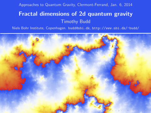
Approaches to Quantum Gravity, Clermont-Ferrand, Jan. 6, 2014
Fractal dimensions of 2d quantum gravityTimothy Budd
Niels Bohr Institute, Copenhagen. [email protected], http://www.nbi.dk/~budd/
Outline
I Introduction to 2d gravity
I Fractal dimensionsI Hausdorff dimension dhI “Teichmuller deformation dimension” dTD
I Hausdorff dimension in dynamical triangulationsI Overview of results in the literatureI Recent numerical results via shortest cycles
I Quantum Liouville gravityI Gaussian free field basicsI Distance in the Liouville metricI Measurement of dhI Derivation of dTD
I Summary & outlook
2D quantum gravity
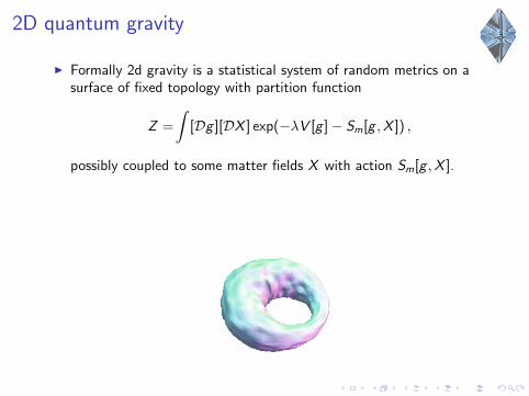
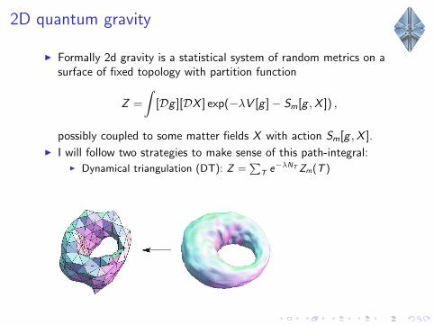
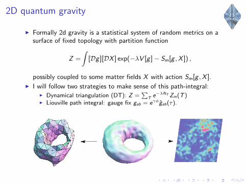
I Formally 2d gravity is a statistical system of random metrics on asurface of fixed topology with partition function
Z =
∫[Dg ][DX ] exp(−λV [g ]− Sm[g ,X ]) ,
possibly coupled to some matter fields X with action Sm[g ,X ].
I I will follow two strategies to make sense of this path-integral:
I Dynamical triangulation (DT): Z =∑
T e−λNTZm(T )
I Liouville path integral: gauge fix gab = eγφgab(τ).
2D quantum gravity
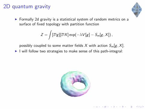
I Formally 2d gravity is a statistical system of random metrics on asurface of fixed topology with partition function
Z =
∫[Dg ][DX ] exp(−λV [g ]− Sm[g ,X ]) ,
possibly coupled to some matter fields X with action Sm[g ,X ].
I I will follow two strategies to make sense of this path-integral:I Dynamical triangulation (DT): Z =
∑T e−λNTZm(T )
I Liouville path integral: gauge fix gab = eγφgab(τ).
2D quantum gravity
I Formally 2d gravity is a statistical system of random metrics on asurface of fixed topology with partition function
Z =
∫[Dg ][DX ] exp(−λV [g ]− Sm[g ,X ]) ,
possibly coupled to some matter fields X with action Sm[g ,X ].
I I will follow two strategies to make sense of this path-integral:I Dynamical triangulation (DT): Z =
∑T e−λNTZm(T )
I Liouville path integral: gauge fix gab = eγφgab(τ).
Hausdorff dimension
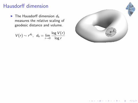
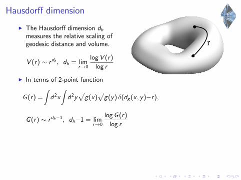
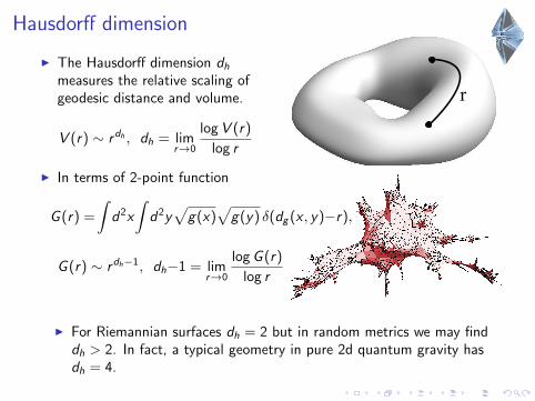
I The Hausdorff dimension dh
measures the relative scaling ofgeodesic distance and volume.
V (r) ∼ rdh , dh = limr→0
log V (r)
log r
I In terms of 2-point function
G (r) =
∫d2x
∫d2y
√g(x)
√g(y) δ(dg (x , y)−r),
G (r) ∼ rdh−1, dh−1 = limr→0
log G (r)
log r
I For Riemannian surfaces dh = 2 but in random metrics we may finddh > 2. In fact, a typical geometry in pure 2d quantum gravity hasdh = 4.

Hausdorff dimension
I The Hausdorff dimension dh
measures the relative scaling ofgeodesic distance and volume.
V (r) ∼ rdh , dh = limr→0
log V (r)
log r
I In terms of 2-point function
G (r) =
∫d2x
∫d2y
√g(x)
√g(y) δ(dg (x , y)−r),
G (r) ∼ rdh−1, dh−1 = limr→0
log G (r)
log r
I For Riemannian surfaces dh = 2 but in random metrics we may finddh > 2. In fact, a typical geometry in pure 2d quantum gravity hasdh = 4.
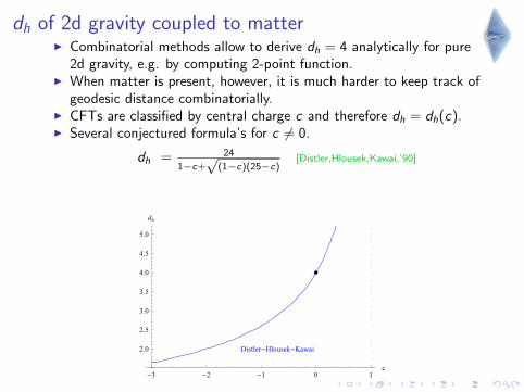
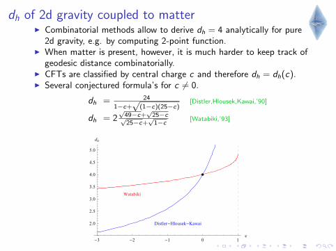
dh of 2d gravity coupled to matterI Combinatorial methods allow to derive dh = 4 analytically for pure
2d gravity, e.g. by computing 2-point function.I When matter is present, however, it is much harder to keep track of
geodesic distance combinatorially.
I CFTs are classified by central charge c and therefore dh = dh(c).I Several conjectured formula’s for c 6= 0.
dh = 24
1−c+√
(1−c)(25−c)[Distler,Hlousek,Kawai,’90]
dh = 2√
49−c+√
25−c√25−c+
√1−c [Watabiki,’93]
dh = 4 [Duplantier,’11]
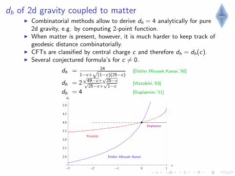
dh of 2d gravity coupled to matterI Combinatorial methods allow to derive dh = 4 analytically for pure
2d gravity, e.g. by computing 2-point function.I When matter is present, however, it is much harder to keep track of
geodesic distance combinatorially.I CFTs are classified by central charge c and therefore dh = dh(c).I Several conjectured formula’s for c 6= 0.
dh = 24
1−c+√
(1−c)(25−c)[Distler,Hlousek,Kawai,’90]
dh = 2√
49−c+√
25−c√25−c+
√1−c [Watabiki,’93]
dh = 4 [Duplantier,’11]
dh of 2d gravity coupled to matter
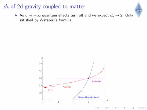
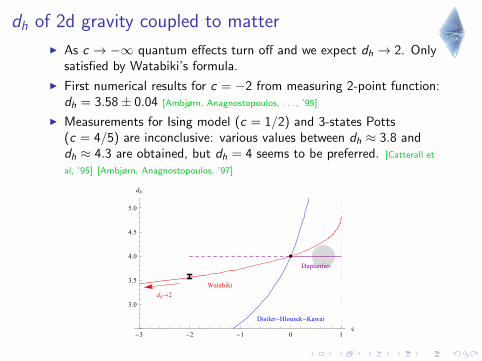
I As c → −∞ quantum effects turn off and we expect dh → 2. Onlysatisfied by Watabiki’s formula.
I First numerical results for c = −2 from measuring 2-point function:dh = 3.58± 0.04 [Ambjørn, Anagnostopoulos, . . . , ’95]
I Measurements for Ising model (c = 1/2) and 3-states Potts(c = 4/5) are inconclusive: various values between dh ≈ 3.8 anddh ≈ 4.3 are obtained, but dh = 4 seems to be preferred. [Catterall et
al, ’95] [Ambjørn, Anagnostopoulos, ’97]
dh of 2d gravity coupled to matter
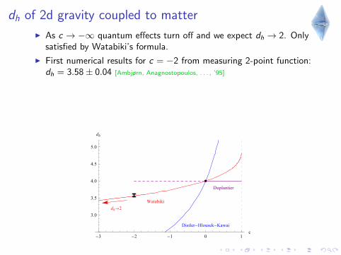
I As c → −∞ quantum effects turn off and we expect dh → 2. Onlysatisfied by Watabiki’s formula.
I First numerical results for c = −2 from measuring 2-point function:dh = 3.58± 0.04 [Ambjørn, Anagnostopoulos, . . . , ’95]
I Measurements for Ising model (c = 1/2) and 3-states Potts(c = 4/5) are inconclusive: various values between dh ≈ 3.8 anddh ≈ 4.3 are obtained, but dh = 4 seems to be preferred. [Catterall et
al, ’95] [Ambjørn, Anagnostopoulos, ’97]
Hausdorff dimension from shortest cycles
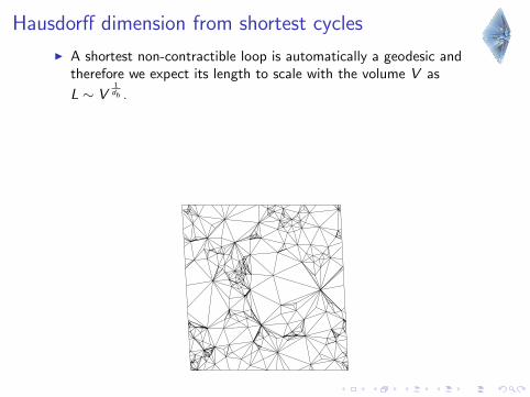
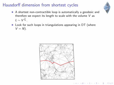
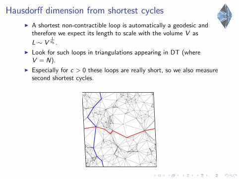
I A shortest non-contractible loop is automatically a geodesic andtherefore we expect its length to scale with the volume V as
L ∼ V1dh .
I Look for such loops in triangulations appearing in DT (whereV = N).
I Especially for c > 0 these loops are really short, so we also measuresecond shortest cycles.
Hausdorff dimension from shortest cycles
I A shortest non-contractible loop is automatically a geodesic andtherefore we expect its length to scale with the volume V as
L ∼ V1dh .
I Look for such loops in triangulations appearing in DT (whereV = N).
I Especially for c > 0 these loops are really short, so we also measuresecond shortest cycles.
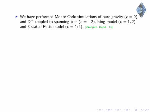
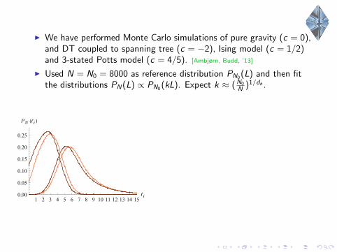
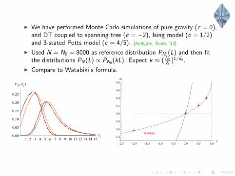
I We have performed Monte Carlo simulations of pure gravity (c = 0),and DT coupled to spanning tree (c = −2), Ising model (c = 1/2)and 3-stated Potts model (c = 4/5). [Ambjørn, Budd, ’13]
I Used N = N0 = 8000 as reference distribution PN0 (L) and then fitthe distributions PN(L) ∝ PN0 (kL). Expect k ≈ (N0
N )1/dh .
I Compare to Watabiki’s formula.
1 2 3 4 5 6 7 8 9 10 11 12 13 14 15
{i0.00
0.05
0.10
0.15
0.20
0.25
PN H{i L
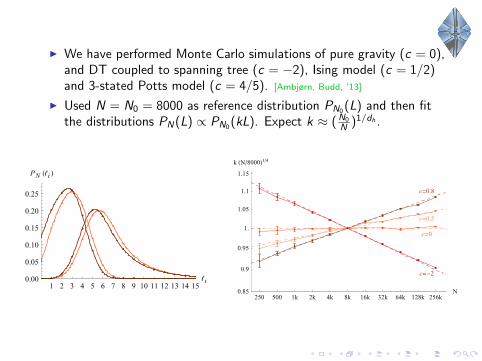
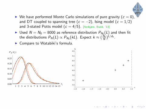
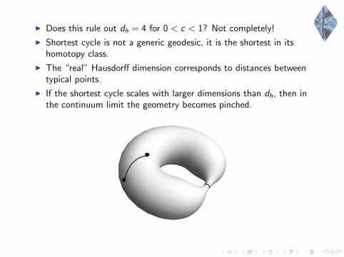
I Does this rule out dh = 4 for 0 < c < 1? Not completely!
I Shortest cycle is not a generic geodesic, it is the shortest in itshomotopy class.
I The “real” Hausdorff dimension corresponds to distances betweentypical points.
I If the shortest cycle scales with larger dimensions than dh, then inthe continuum limit the geometry becomes pinched.
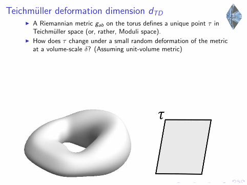
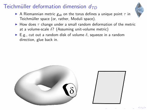
Teichmuller deformation dimension dTD
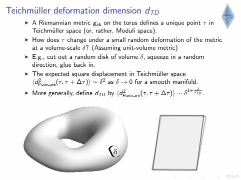
I A Riemannian metric gab on the torus defines a unique point τ inTeichmuller space (or, rather, Moduli space).
I How does τ change under a small random deformation of the metricat a volume-scale δ? (Assuming unit-volume metric)
I E.g., cut out a random disk of volume δ, squeeze in a randomdirection, glue back in.
I The expected square displacement in Teichmuller space〈d2
Poincare(τ, τ + ∆τ)〉 ∼ δ2 as δ → 0 for a smooth manifold.
I More generally, define dTD by 〈d2Poincare(τ, τ + ∆τ)〉 ∼ δ1+ 2
dTD .
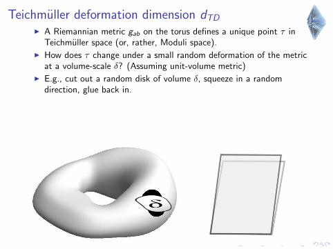
Teichmuller deformation dimension dTD
I A Riemannian metric gab on the torus defines a unique point τ inTeichmuller space (or, rather, Moduli space).
I How does τ change under a small random deformation of the metricat a volume-scale δ? (Assuming unit-volume metric)
I E.g., cut out a random disk of volume δ, squeeze in a randomdirection, glue back in.
I The expected square displacement in Teichmuller space〈d2
Poincare(τ, τ + ∆τ)〉 ∼ δ2 as δ → 0 for a smooth manifold.
I More generally, define dTD by 〈d2Poincare(τ, τ + ∆τ)〉 ∼ δ1+ 2
dTD .
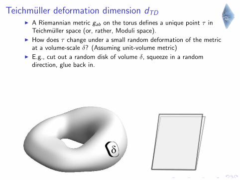
Teichmuller deformation dimension dTD
I A Riemannian metric gab on the torus defines a unique point τ inTeichmuller space (or, rather, Moduli space).
I How does τ change under a small random deformation of the metricat a volume-scale δ? (Assuming unit-volume metric)
I E.g., cut out a random disk of volume δ, squeeze in a randomdirection, glue back in.
I The expected square displacement in Teichmuller space〈d2
Poincare(τ, τ + ∆τ)〉 ∼ δ2 as δ → 0 for a smooth manifold.
I More generally, define dTD by 〈d2Poincare(τ, τ + ∆τ)〉 ∼ δ1+ 2
dTD .
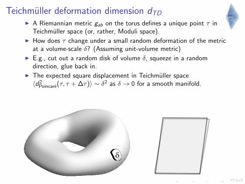
Teichmuller deformation dimension dTD
I A Riemannian metric gab on the torus defines a unique point τ inTeichmuller space (or, rather, Moduli space).
I How does τ change under a small random deformation of the metricat a volume-scale δ? (Assuming unit-volume metric)
I E.g., cut out a random disk of volume δ, squeeze in a randomdirection, glue back in.
I The expected square displacement in Teichmuller space〈d2
Poincare(τ, τ + ∆τ)〉 ∼ δ2 as δ → 0 for a smooth manifold.
I More generally, define dTD by 〈d2Poincare(τ, τ + ∆τ)〉 ∼ δ1+ 2
dTD .
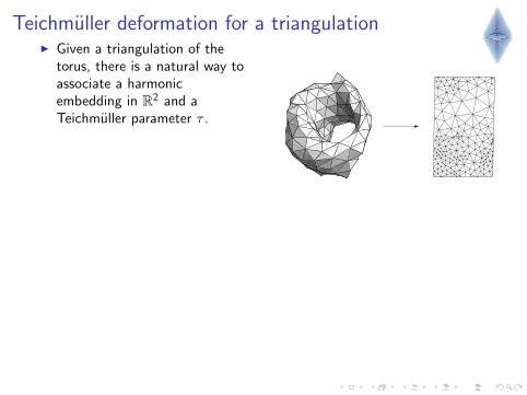
Teichmuller deformation for a triangulationI Given a triangulation of the
torus, there is a natural way toassociate a harmonicembedding in R2 and aTeichmuller parameter τ .
I Replace edges by ideal springsand find equilibrium.
I Find linear transformation thatminimizes energy while fixingthe volume.
Τ
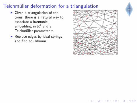
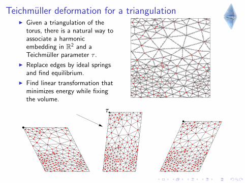
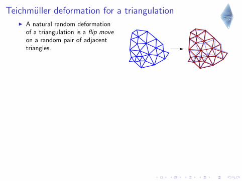
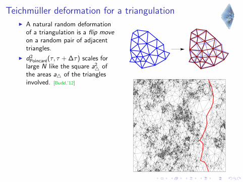
Teichmuller deformation for a triangulationI A natural random deformation
of a triangulation is a flip moveon a random pair of adjacenttriangles.
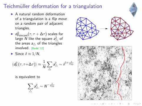
I d2Poincare(τ, τ + ∆τ) scales for
large N like the square a24 of
the areas a4 of the trianglesinvolved. [Budd,’12]
I Since δ ≈ 1/N,
〈d2P.(τ, τ+∆τ)〉 ≈ 1
N
∑4
a24 ∼ δ
1+ 2dTD
is equivalent to∑4
a24 ∼ N
− 2dTD
Teichmuller deformation for a triangulationI A natural random deformation
of a triangulation is a flip moveon a random pair of adjacenttriangles.
I d2Poincare(τ, τ + ∆τ) scales for
large N like the square a24 of
the areas a4 of the trianglesinvolved. [Budd,’12]
I Since δ ≈ 1/N,
〈d2P.(τ, τ+∆τ)〉 ≈ 1
N
∑4
a24 ∼ δ
1+ 2dTD
is equivalent to∑4
a24 ∼ N
− 2dTD
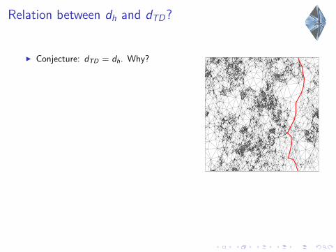
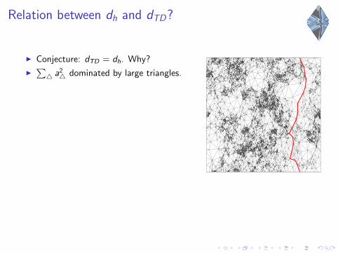
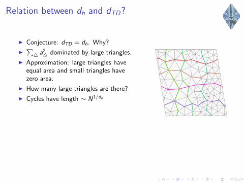
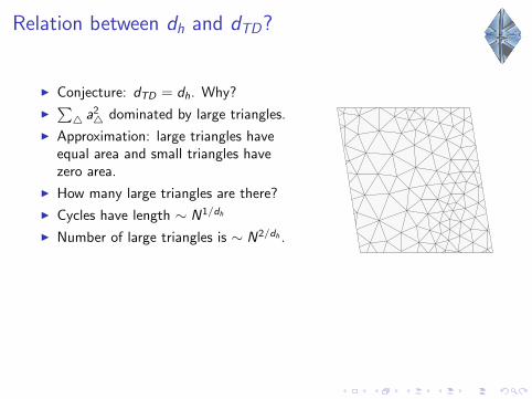
Relation between dh and dTD?
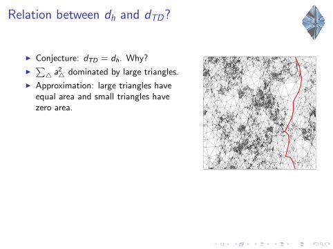
I Conjecture: dTD = dh. Why?
I∑4 a24 dominated by large triangles.
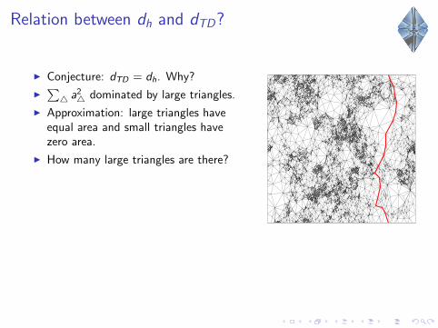
I Approximation: large triangles haveequal area and small triangles havezero area.
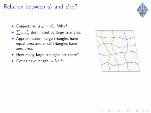
I How many large triangles are there?
I Cycles have length ∼ N1/dh
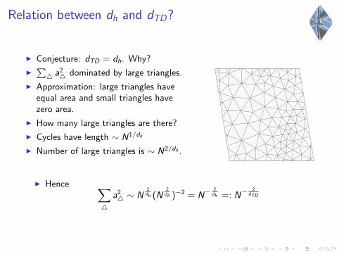
I Number of large triangles is ∼ N2/dh .
I Hence ∑4
a24 ∼ N
2dh (N
2dh )−2 = N
− 2dh =: N
− 2dTD
Relation between dh and dTD?
I Conjecture: dTD = dh. Why?
I∑4 a24 dominated by large triangles.
I Approximation: large triangles haveequal area and small triangles havezero area.
I How many large triangles are there?
I Cycles have length ∼ N1/dh
I Number of large triangles is ∼ N2/dh .
I Hence ∑4
a24 ∼ N
2dh (N
2dh )−2 = N
− 2dh =: N
− 2dTD
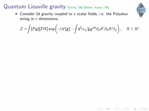
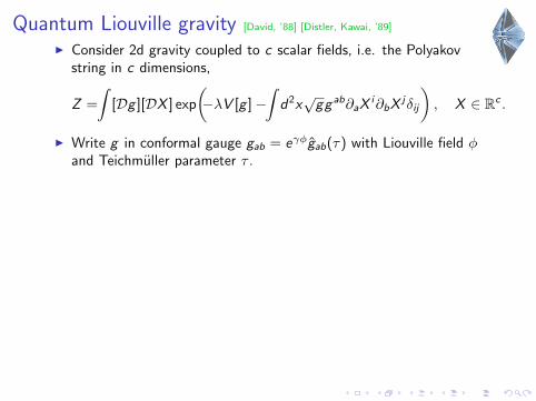
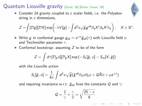
Quantum Liouville gravity [David, ’88] [Distler, Kawai, ’89]
I Consider 2d gravity coupled to c scalar fields, i.e. the Polyakovstring in c dimensions,
Z =
∫[Dg ][DX ] exp
(−λV [g ]−
∫d2x√
gg ab∂aX i∂bX jδij
), X ∈ Rc .
I Write g in conformal gauge gab = eγφgab(τ) with Liouville field φand Teichmuller parameter τ .
I Conformal bootstrap: assuming Z to be of the form
Z =
∫dτ [Dgφ][DgX ] exp (−SL[g , φ]− Sm[X , g ])
with the Liouville action
SL[g , φ] =1
4π
∫d2x
√g(g ab∂aφ∂bφ+ QRφ+ µeγφ)
and requiring invariance w.r.t. gab fixes the constants Q and γ:
Q =2
γ+γ
2=
√25− c
6
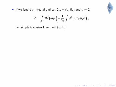
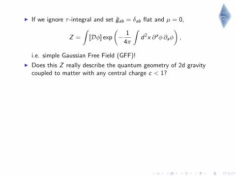
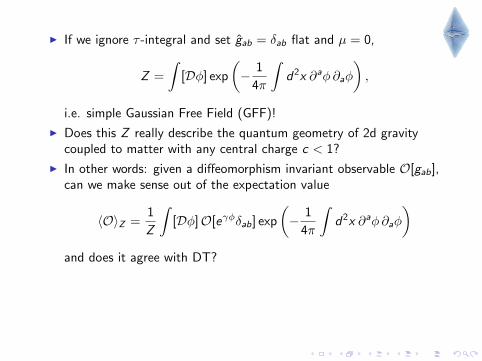
I If we ignore τ -integral and set gab = δab flat and µ = 0,
Z =
∫[Dφ] exp
(− 1
4π
∫d2x ∂aφ∂aφ
),
i.e. simple Gaussian Free Field (GFF)!
I Does this Z really describe the quantum geometry of 2d gravitycoupled to matter with any central charge c < 1?
I In other words: given a diffeomorphism invariant observable O[gab],can we make sense out of the expectation value
〈O〉Z =1
Z
∫[Dφ]O[eγφδab] exp
(− 1
4π
∫d2x ∂aφ∂aφ
)and does it agree with DT?
I Care required: eγφδab is almost surely not a Riemannian metric!Need to take into account the fractal properties of the geometry andregularize appropriately.
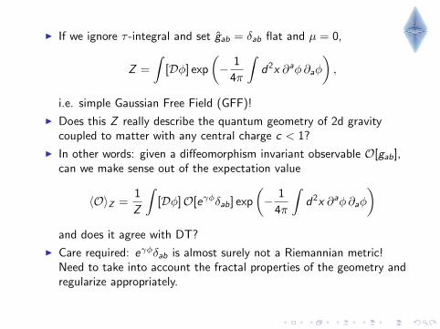
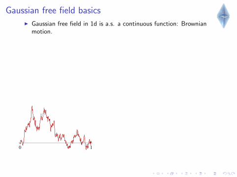
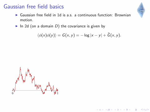
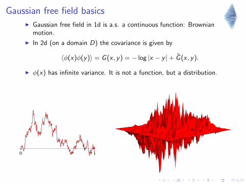
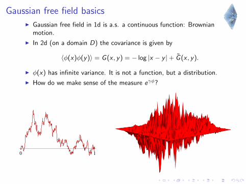
Gaussian free field basicsI Gaussian free field in 1d is a.s. a continuous function: Brownian
motion.
I In 2d (on a domain D) the covariance is given by
〈φ(x)φ(y)〉 = G (x , y) = − log |x − y |+ G (x , y).
I φ(x) has infinite variance. It is not a function, but a distribution.
I How do we make sense of the measure eγφ?
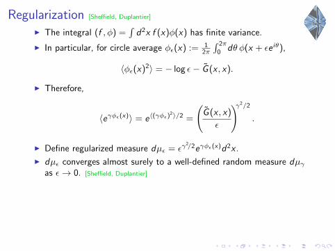
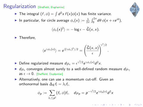
Regularization [Sheffield, Duplantier]
I The integral (f , φ) =∫
d2x f (x)φ(x) has finite variance.
I In particular, for circle average φε(x) := 12π
∫ 2π
0dθ φ(x + εe iθ),
〈φε(x)2〉 = − log ε− G (x , x).
I Therefore,
〈eγφε(x)〉 = e〈(γφε)2〉/2 =
(G (x , x)
ε
)γ2/2
.
I Define regularized measure dµε = εγ2/2eγφε(x)d2x .
I dµε converges almost surely to a well-defined random measure dµγas ε→ 0. [Sheffield, Duplantier]
I Alternatively, one can use a momentum cut-off. Given anorthonormal basis ∆E fi = λi fi ,
φp :=∑λi≤p2
(fi , φ)fi , dµp = p−γ2/2eγφp(x)d2x
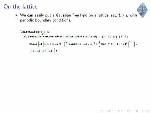
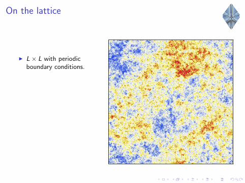
On the latticeI We can easily put a Gaussian free field on a lattice, say, L× L with
periodic boundary conditions.
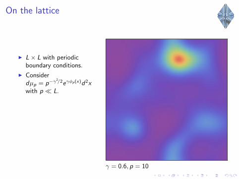
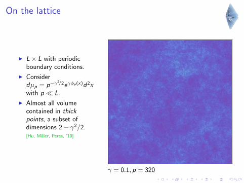
I L× L with periodicboundary conditions.
I Considerdµp = p−γ
2/2eγφp(x)d2xwith p � L.
I Almost all volumecontained in thickpoints, a subset ofdimensions 2− γ2/2.[Hu, Miller, Peres, ’10]
On the lattice
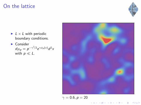
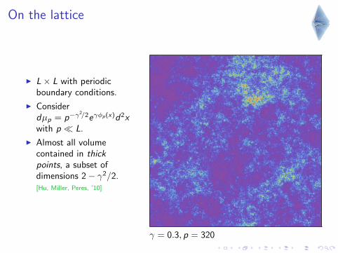
I L× L with periodicboundary conditions.
I Considerdµp = p−γ
2/2eγφp(x)d2xwith p � L.
I Almost all volumecontained in thickpoints, a subset ofdimensions 2− γ2/2.[Hu, Miller, Peres, ’10]
p = 0
On the lattice
I L× L with periodicboundary conditions.
I Considerdµp = p−γ
2/2eγφp(x)d2xwith p � L.
I Almost all volumecontained in thickpoints, a subset ofdimensions 2− γ2/2.[Hu, Miller, Peres, ’10]
γ = 0.6, p = 10
On the lattice
I L× L with periodicboundary conditions.
I Considerdµp = p−γ
2/2eγφp(x)d2xwith p � L.
I Almost all volumecontained in thickpoints, a subset ofdimensions 2− γ2/2.[Hu, Miller, Peres, ’10]
γ = 0.6, p = 20

On the lattice
I L× L with periodicboundary conditions.
I Considerdµp = p−γ
2/2eγφp(x)d2xwith p � L.
I Almost all volumecontained in thickpoints, a subset ofdimensions 2− γ2/2.[Hu, Miller, Peres, ’10]
γ = 0.6, p = 40

On the lattice
I L× L with periodicboundary conditions.
I Considerdµp = p−γ
2/2eγφp(x)d2xwith p � L.
I Almost all volumecontained in thickpoints, a subset ofdimensions 2− γ2/2.[Hu, Miller, Peres, ’10]
γ = 0.6, p = 80
On the lattice
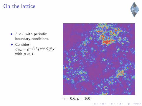
I L× L with periodicboundary conditions.
I Considerdµp = p−γ
2/2eγφp(x)d2xwith p � L.
I Almost all volumecontained in thickpoints, a subset ofdimensions 2− γ2/2.[Hu, Miller, Peres, ’10]
γ = 0.6, p = 160
On the lattice
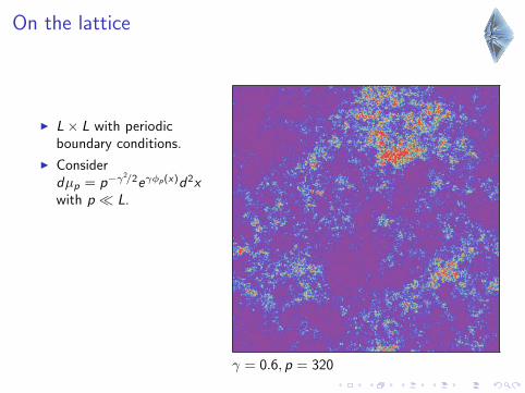
I L× L with periodicboundary conditions.
I Considerdµp = p−γ
2/2eγφp(x)d2xwith p � L.
I Almost all volumecontained in thickpoints, a subset ofdimensions 2− γ2/2.[Hu, Miller, Peres, ’10]
γ = 0.6, p = 320
On the lattice
I L× L with periodicboundary conditions.
I Considerdµp = p−γ
2/2eγφp(x)d2xwith p � L.
I Almost all volumecontained in thickpoints, a subset ofdimensions 2− γ2/2.[Hu, Miller, Peres, ’10]
γ = 0.1, p = 320
On the lattice
I L× L with periodicboundary conditions.
I Considerdµp = p−γ
2/2eγφp(x)d2xwith p � L.
I Almost all volumecontained in thickpoints, a subset ofdimensions 2− γ2/2.[Hu, Miller, Peres, ’10]
γ = 0.3, p = 320

On the lattice
I L× L with periodicboundary conditions.
I Considerdµp = p−γ
2/2eγφp(x)d2xwith p � L.
I Almost all volumecontained in thickpoints, a subset ofdimensions 2− γ2/2.[Hu, Miller, Peres, ’10]
γ = 0.6, p = 320
On the lattice
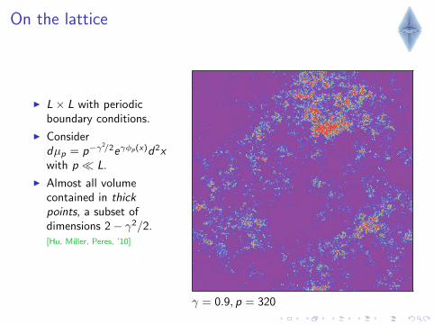
I L× L with periodicboundary conditions.
I Considerdµp = p−γ
2/2eγφp(x)d2xwith p � L.
I Almost all volumecontained in thickpoints, a subset ofdimensions 2− γ2/2.[Hu, Miller, Peres, ’10]
γ = 0.9, p = 320
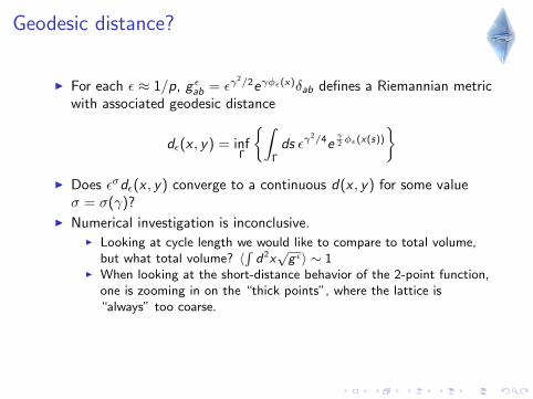
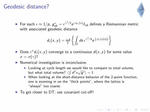
Geodesic distance?
I For each ε ≈ 1/p, g εab = εγ2/2eγφε(x)δab defines a Riemannian metric
with associated geodesic distance
dε(x , y) = infΓ
{∫Γ
ds εγ2/4e
γ2 φε(x(s))
}I Does εσdε(x , y) converge to a continuous d(x , y) for some valueσ = σ(γ)?
I Numerical investigation is inconclusive.I Looking at cycle length we would like to compare to total volume,
but what total volume? 〈∫d2x√g ε〉 ∼ 1
I When looking at the short-distance behavior of the 2-point function,one is zooming in on the “thick points”, where the lattice is“always” too coarse.
I To get closer to DT: use covariant cut-off!
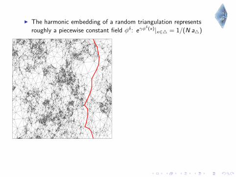
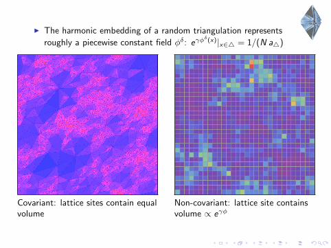
I The harmonic embedding of a random triangulation represents
roughly a piecewise constant field φδ: eγφδ(x)|x∈4 = 1/(N a4)
Covariant: lattice sites contain equalvolume
Non-covariant: lattice site containsvolume ∝ eγφ
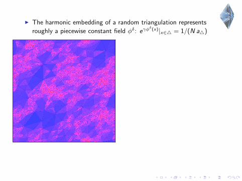
I The harmonic embedding of a random triangulation represents
roughly a piecewise constant field φδ: eγφδ(x)|x∈4 = 1/(N a4)
Covariant: lattice sites contain equalvolume
Non-covariant: lattice site containsvolume ∝ eγφ
I The harmonic embedding of a random triangulation represents
roughly a piecewise constant field φδ: eγφδ(x)|x∈4 = 1/(N a4)
Covariant: lattice sites contain equalvolume
Non-covariant: lattice site containsvolume ∝ eγφ
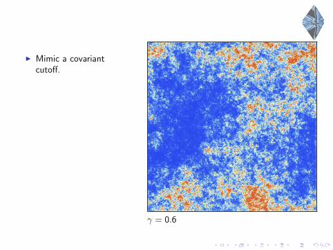
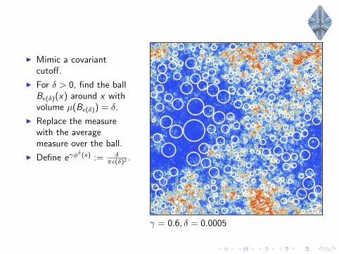
I Mimic a covariantcutoff.
I For δ > 0, find the ballBε(δ)(x) around x withvolume µ(Bε(δ)) = δ.
I Replace the measurewith the averagemeasure over the ball.
I Define eγφδ(x) := δ
πε(δ)2 .
I Compare to DT:δ ∼ 1/N
γ = 0.6
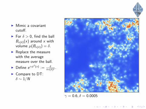
I Mimic a covariantcutoff.
I For δ > 0, find the ballBε(δ)(x) around x withvolume µ(Bε(δ)) = δ.
I Replace the measurewith the averagemeasure over the ball.
I Define eγφδ(x) := δ
πε(δ)2 .
I Compare to DT:δ ∼ 1/N
γ = 0.6, δ = 0.01
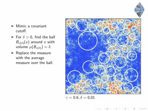
I Mimic a covariantcutoff.
I For δ > 0, find the ballBε(δ)(x) around x withvolume µ(Bε(δ)) = δ.
I Replace the measurewith the averagemeasure over the ball.
I Define eγφδ(x) := δ
πε(δ)2 .
I Compare to DT:δ ∼ 1/N
γ = 0.6, δ = 0.01
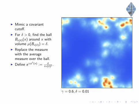
I Mimic a covariantcutoff.
I For δ > 0, find the ballBε(δ)(x) around x withvolume µ(Bε(δ)) = δ.
I Replace the measurewith the averagemeasure over the ball.
I Define eγφδ(x) := δ
πε(δ)2 .
I Compare to DT:δ ∼ 1/N
γ = 0.6, δ = 0.0005
I Mimic a covariantcutoff.
I For δ > 0, find the ballBε(δ)(x) around x withvolume µ(Bε(δ)) = δ.
I Replace the measurewith the averagemeasure over the ball.
I Define eγφδ(x) := δ
πε(δ)2 .
I Compare to DT:δ ∼ 1/N
γ = 0.6, δ = 0.0005
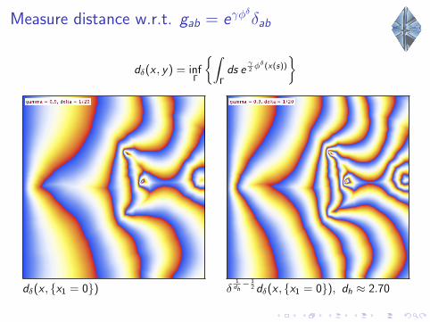
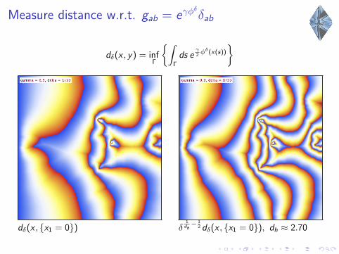
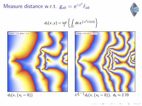
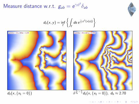
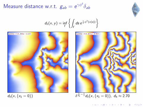
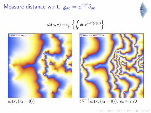
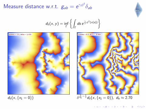
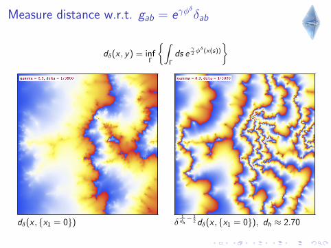
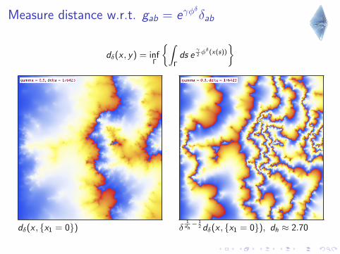
Measure distance w.r.t. gab = eγφδ
δab
dδ(x , y) = infΓ
{∫Γ
ds eγ2 φ
δ(x(s))
}
dδ(x , {x1 = 0}) δ1dh− 1
2 dδ(x , {x1 = 0}), dh ≈ 2.70
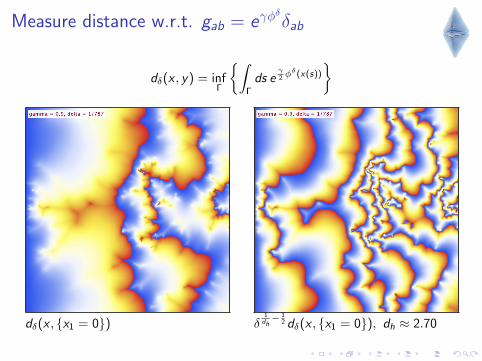
Measure distance w.r.t. gab = eγφδ
δab
dδ(x , y) = infΓ
{∫Γ
ds eγ2 φ
δ(x(s))
}
dδ(x , {x1 = 0}) δ1dh− 1
2 dδ(x , {x1 = 0}), dh ≈ 2.70
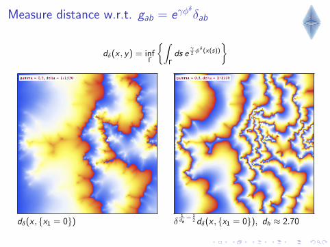
Measure distance w.r.t. gab = eγφδ
δab
dδ(x , y) = infΓ
{∫Γ
ds eγ2 φ
δ(x(s))
}
dδ(x , {x1 = 0}) δ1dh− 1
2 dδ(x , {x1 = 0}), dh ≈ 2.70
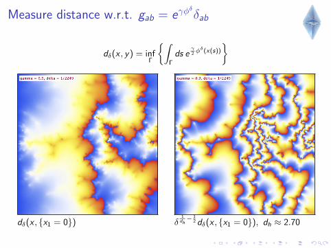
Measure distance w.r.t. gab = eγφδ
δab
dδ(x , y) = infΓ
{∫Γ
ds eγ2 φ
δ(x(s))
}
dδ(x , {x1 = 0}) δ1dh− 1
2 dδ(x , {x1 = 0}), dh ≈ 2.70
Measure distance w.r.t. gab = eγφδ
δab
dδ(x , y) = infΓ
{∫Γ
ds eγ2 φ
δ(x(s))
}
dδ(x , {x1 = 0}) δ1dh− 1
2 dδ(x , {x1 = 0}), dh ≈ 2.70
Measure distance w.r.t. gab = eγφδ
δab
dδ(x , y) = infΓ
{∫Γ
ds eγ2 φ
δ(x(s))
}
dδ(x , {x1 = 0}) δ1dh− 1
2 dδ(x , {x1 = 0}), dh ≈ 2.70
Measure distance w.r.t. gab = eγφδ
δab
dδ(x , y) = infΓ
{∫Γ
ds eγ2 φ
δ(x(s))
}
dδ(x , {x1 = 0}) δ1dh− 1
2 dδ(x , {x1 = 0}), dh ≈ 2.70
Measure distance w.r.t. gab = eγφδ
δab
dδ(x , y) = infΓ
{∫Γ
ds eγ2 φ
δ(x(s))
}
dδ(x , {x1 = 0}) δ1dh− 1
2 dδ(x , {x1 = 0}), dh ≈ 2.70
Measure distance w.r.t. gab = eγφδ
δab
dδ(x , y) = infΓ
{∫Γ
ds eγ2 φ
δ(x(s))
}
dδ(x , {x1 = 0}) δ1dh− 1
2 dδ(x , {x1 = 0}), dh ≈ 2.70
Measure distance w.r.t. gab = eγφδ
δab
dδ(x , y) = infΓ
{∫Γ
ds eγ2 φ
δ(x(s))
}
dδ(x , {x1 = 0}) δ1dh− 1
2 dδ(x , {x1 = 0}), dh ≈ 2.70
Measure distance w.r.t. gab = eγφδ
δab
dδ(x , y) = infΓ
{∫Γ
ds eγ2 φ
δ(x(s))
}
dδ(x , {x1 = 0}) δ1dh− 1
2 dδ(x , {x1 = 0}), dh ≈ 2.70
Measure distance w.r.t. gab = eγφδ
δab
dδ(x , y) = infΓ
{∫Γ
ds eγ2 φ
δ(x(s))
}
dδ(x , {x1 = 0}) δ1dh− 1
2 dδ(x , {x1 = 0}), dh ≈ 2.70
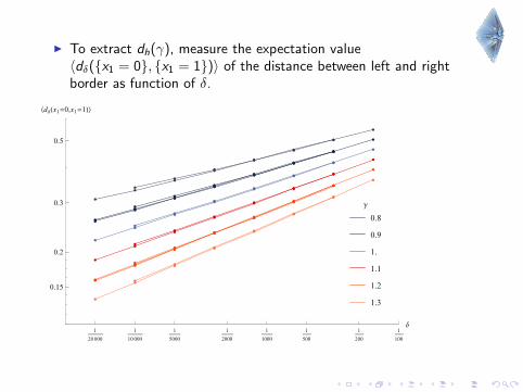
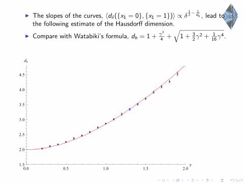
I To extract dh(γ), measure the expectation value〈dδ({x1 = 0}, {x1 = 1})〉 of the distance between left and rightborder as function of δ.
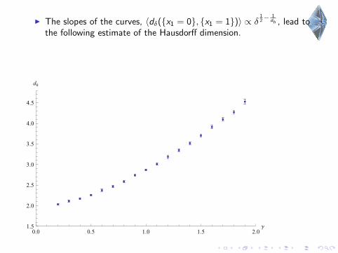
I The slopes of the curves, 〈dδ({x1 = 0}, {x1 = 1})〉 ∝ δ12−
1dh , lead to
the following estimate of the Hausdorff dimension.
I Compare with Watabiki’s formula, dh = 1 + γ2
4 +√
1 + 32γ
2 + 116γ
4.
I Can we understand where this formula comes from?
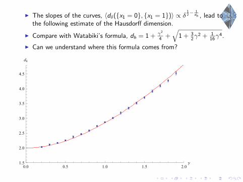
I The slopes of the curves, 〈dδ({x1 = 0}, {x1 = 1})〉 ∝ δ12−
1dh , lead to
the following estimate of the Hausdorff dimension.
I Compare with Watabiki’s formula, dh = 1 + γ2
4 +√
1 + 32γ
2 + 116γ
4.
I Can we understand where this formula comes from?
I The slopes of the curves, 〈dδ({x1 = 0}, {x1 = 1})〉 ∝ δ12−
1dh , lead to
the following estimate of the Hausdorff dimension.
I Compare with Watabiki’s formula, dh = 1 + γ2
4 +√
1 + 32γ
2 + 116γ
4.
I Can we understand where this formula comes from?
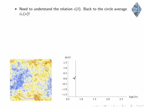
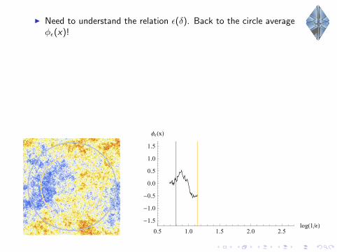
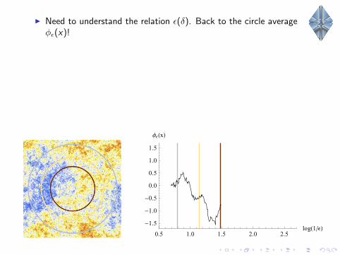
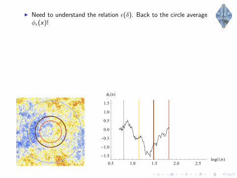
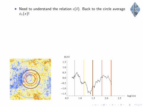
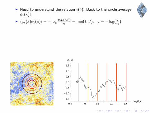
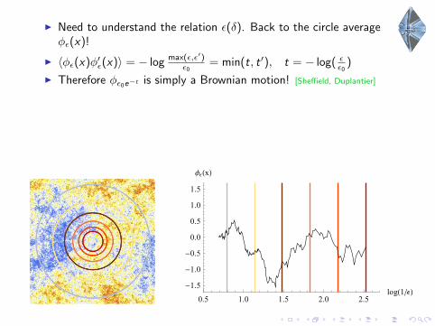
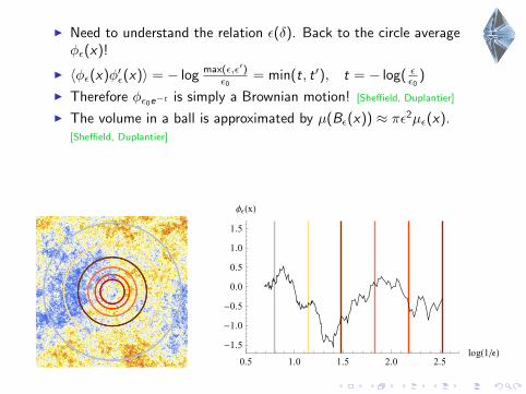
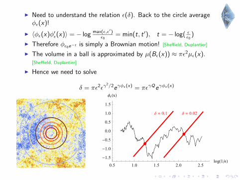
I Need to understand the relation ε(δ). Back to the circle averageφε(x)!
I 〈φε(x)φ′ε(x)〉 = − log max(ε,ε′)ε0
= min(t, t ′), t = − log( εε0)
I Therefore φε0e−t is simply a Brownian motion! [Sheffield, Duplantier]
I The volume in a ball is approximated by µ(Bε(x)) ≈ πε2µε(x).[Sheffield, Duplantier]
I Hence we need to solve
δ = πε2εγ2/2eγφε(x) = πεγQeγφε(x)
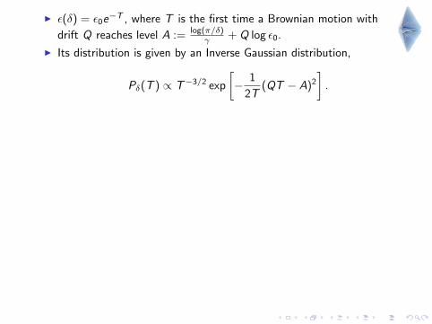
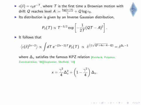
I ε(δ) = ε0e−T , where T is the first time a Brownian motion with
drift Q reaches level A := log(π/δ)γ + Q log ε0.
I Its distribution is given by an Inverse Gaussian distribution,
Pδ(T ) ∝ T−3/2 exp
[− 1
2T(QT − A)2
].
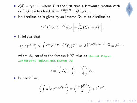
I It follows that⟨ε(δ)2x−2
⟩∝∫
dT e−(2x−2)TPδ(T ) ∝ δ1γ (√Q2+4x−4−Q) = δ∆x−1
where ∆x satisfies the famous KPZ relation [Knizhnik, Polyakov,
Zamolodchikov, ’88][Duplantier, Sheffield, ’10]
x =γ2
4∆2
x +
(1− γ2
4
)∆x .
I In particular,⟨∫d2x e−γφ
δ(x)
⟩=
⟨πε(δ)2
δ
⟩∝ δ∆2−2.
I ε(δ) = ε0e−T , where T is the first time a Brownian motion with
drift Q reaches level A := log(π/δ)γ + Q log ε0.
I Its distribution is given by an Inverse Gaussian distribution,
Pδ(T ) ∝ T−3/2 exp
[− 1
2T(QT − A)2
].
I It follows that⟨ε(δ)2x−2
⟩∝∫
dT e−(2x−2)TPδ(T ) ∝ δ1γ (√Q2+4x−4−Q) = δ∆x−1
where ∆x satisfies the famous KPZ relation [Knizhnik, Polyakov,
Zamolodchikov, ’88][Duplantier, Sheffield, ’10]
x =γ2
4∆2
x +
(1− γ2
4
)∆x .
I In particular,⟨∫d2x e−γφ
δ(x)
⟩=
⟨πε(δ)2
δ
⟩∝ δ∆2−2.
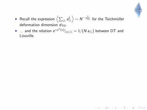
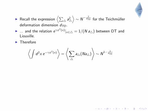
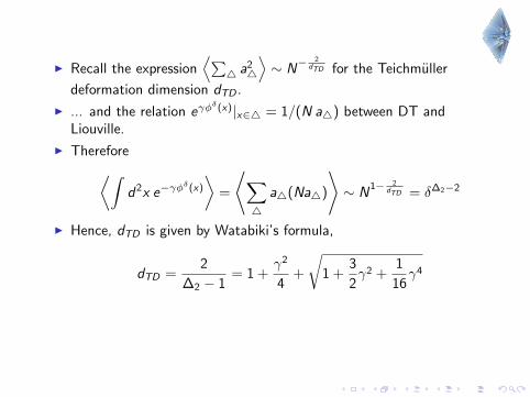
I Recall the expression⟨∑
4 a24
⟩∼ N
− 2dTD for the Teichmuller
deformation dimension dTD .
I ... and the relation eγφδ(x)|x∈4 = 1/(N a4) between DT and
Liouville.
I Therefore⟨∫d2x e−γφ
δ(x)
⟩=
⟨∑4
a4(Na4)
⟩∼ N
1− 2dTD
= δ∆2−2
I Hence, dTD is given by Watabiki’s formula,
dTD =2
∆2 − 1= 1 +
γ2
4+
√1 +
3
2γ2 +
1
16γ4
I Recall the expression⟨∑
4 a24
⟩∼ N
− 2dTD for the Teichmuller
deformation dimension dTD .
I ... and the relation eγφδ(x)|x∈4 = 1/(N a4) between DT and
Liouville.
I Therefore⟨∫d2x e−γφ
δ(x)
⟩=
⟨∑4
a4(Na4)
⟩∼ N
1− 2dTD = δ∆2−2
I Hence, dTD is given by Watabiki’s formula,
dTD =2
∆2 − 1= 1 +
γ2
4+
√1 +
3
2γ2 +
1
16γ4
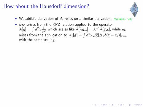
How about the Hausdorff dimension?
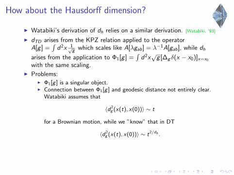
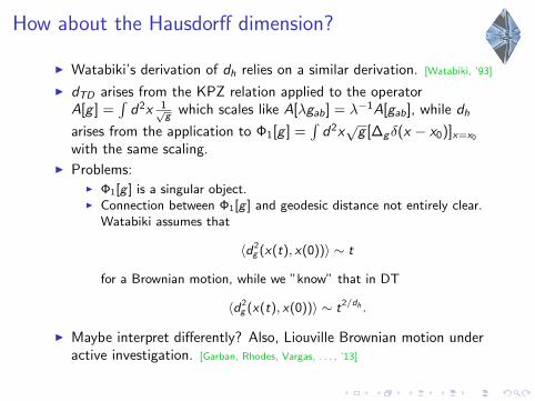
I Watabiki’s derivation of dh relies on a similar derivation. [Watabiki, ’93]
I dTD arises from the KPZ relation applied to the operatorA[g ] =
∫d2x 1√
g which scales like A[λgab] = λ−1A[gab], while dh
arises from the application to Φ1[g ] =∫
d2x√
g [∆gδ(x − x0)]x=x0
with the same scaling.
I Problems:I Φ1[g ] is a singular object.I Connection between Φ1[g ] and geodesic distance not entirely clear.
Watabiki assumes that
〈d2g (x(t), x(0))〉 ∼ t
for a Brownian motion, while we ”know” that in DT
〈d2g (x(t), x(0))〉 ∼ t2/dh .
I Maybe interpret differently? Also, Liouville Brownian motion underactive investigation. [Garban, Rhodes, Vargas, . . . , ’13]
How about the Hausdorff dimension?
I Watabiki’s derivation of dh relies on a similar derivation. [Watabiki, ’93]
I dTD arises from the KPZ relation applied to the operatorA[g ] =
∫d2x 1√
g which scales like A[λgab] = λ−1A[gab], while dh
arises from the application to Φ1[g ] =∫
d2x√
g [∆gδ(x − x0)]x=x0
with the same scaling.
I Problems:I Φ1[g ] is a singular object.I Connection between Φ1[g ] and geodesic distance not entirely clear.
Watabiki assumes that
〈d2g (x(t), x(0))〉 ∼ t
for a Brownian motion, while we ”know” that in DT
〈d2g (x(t), x(0))〉 ∼ t2/dh .
I Maybe interpret differently? Also, Liouville Brownian motion underactive investigation. [Garban, Rhodes, Vargas, . . . , ’13]
Summary & outlookI Summary:
I Numerical simulations both in DT and in Liouville gravity on thelattice support Watabiki’s formula for the Hausdorff dimension forc < 1,
dh = 2
√49− c +
√25− c√
25− c +√
1− c.
I A different dimension, the Teichmuller deformation dimension dTD ,can be seen to be given by Watabiki’s formula and therefore likelycoincides with dh.
I Outlook/questions:
I Make sense of Watabiki’s derivation and preferably turn it into aproof.
I Relation with Quantum Loewner Evolution? [Miller,Sheffield,’13]
I Can the Teichmuller deformation dimension be defined moregenerally? On S2 or higher genus?
I Is it possible that shortest cycles and generic geodesic distances scaledifferently? Then dh = 4 for 0 < c < 1 is not yet ruled out, but thecontinuum random surface would be pinched.
Thanks! Questions? Slides available at http://www.nbi.dk/~budd/
Summary & outlookI Summary:
I Numerical simulations both in DT and in Liouville gravity on thelattice support Watabiki’s formula for the Hausdorff dimension forc < 1,
dh = 2
√49− c +
√25− c√
25− c +√
1− c.
I A different dimension, the Teichmuller deformation dimension dTD ,can be seen to be given by Watabiki’s formula and therefore likelycoincides with dh.
I Outlook/questions:I Make sense of Watabiki’s derivation and preferably turn it into a
proof.
I Relation with Quantum Loewner Evolution? [Miller,Sheffield,’13]
I Can the Teichmuller deformation dimension be defined moregenerally? On S2 or higher genus?
I Is it possible that shortest cycles and generic geodesic distances scaledifferently? Then dh = 4 for 0 < c < 1 is not yet ruled out, but thecontinuum random surface would be pinched.
Thanks! Questions? Slides available at http://www.nbi.dk/~budd/
Summary & outlookI Summary:
I Numerical simulations both in DT and in Liouville gravity on thelattice support Watabiki’s formula for the Hausdorff dimension forc < 1,
dh = 2
√49− c +
√25− c√
25− c +√
1− c.
I A different dimension, the Teichmuller deformation dimension dTD ,can be seen to be given by Watabiki’s formula and therefore likelycoincides with dh.
I Outlook/questions:I Make sense of Watabiki’s derivation and preferably turn it into a
proof.I Relation with Quantum Loewner Evolution? [Miller,Sheffield,’13]
I Can the Teichmuller deformation dimension be defined moregenerally? On S2 or higher genus?
I Is it possible that shortest cycles and generic geodesic distances scaledifferently? Then dh = 4 for 0 < c < 1 is not yet ruled out, but thecontinuum random surface would be pinched.
Thanks! Questions? Slides available at http://www.nbi.dk/~budd/