fpga based area efficient 64-point fft using mac … based area efficient 64-point fft using mac...

International Journal of Recent Trends in Electrical & Electronics Engg., Dec. 2013.

©IJRTE ISSN: 2231-6612

Volume 3, Issue 1, pg: aa-aa | 1

FPGA Based Area Efficient 64-Point FFT Using MAC

Algorithm

1Rajesh Mehra , 2Pooja Kataria

1,2National Institute of Technical Teachers, Training and Research,

Chandigarh 160019, India

ABSTRACT It is important to develop a high-performance FFT processor to meet the requirements of real time and low cost

in many different systems. So a 64-point FFT is realized by decomposing it into a two-dimensional structure of

8-point FFTs. This approach reduces the number of required complex multiplications as compared to the

conventional radix-2 64-point FFT algorithm. The proposed 64-point FFT is designed and simulated with Matlab

and Xilinx DSP Tools, synthesized with Xilinx Synthesis Tool (XST), and implemented on Spartan 3E based

xc3s500 FPGA device. The results show that proposed FFT consumes very less resources in terms of slices, flip

flops and multipliers to provide cost effective solution for DSP applications.

INDEX TERMS— Butterfly, DFT, Fast Fourier Transform (FFT), FPGA, VHDL

I. INTRODUCTION

One of the most widely used technique in science and engineering is the concept of Fourier Transform

and other algorithms based on it. In signal processing, it is primarily used to convert an input signal in

time domain into frequency domain and vice-versa. In the world of digital, signals are sampled in time

domain[1],[2]. So, we have Discrete Fourier Transform (DFT) in the digital world. DFT is applied on a

discrete input signal and we get the frequency characteristics of the signal as the output. Performing

inverse DFT, which has a mathematical form very similar to the DFT, on the frequency domain result

gives back the signal in the time domain. This means that the signal when converted into frequency

domain will give us the various frequency components of the input signal and then can be used to

remove certain unwanted frequency components.

Discrete Fourier Transform is a very computationally intensive process that is based on summation a

finite series of products of input signal values and trigonometric functions. Its time complexity of the

algorithm in O(n2).To increase the performance, several algorithms were proposed which can be

implemented in hardware or software. These set of algorithms are known as Fast Fourier Transforms

(FFT). The first major FFT algorithm was proposed by Cooley and Tukey [3]. Many FFT algorithms

were proposed with a time complexity of O(nlogn).

The FFT hardware is heavily constrained by the area and speed requirement and thus the focus is to

minimize these two parameters without sacrificing the performance. For large FFT sizes the major

portion of the area for the FFT hardware generally comes from the storage/memory elements for the

twiddle factor tables and pipeline registers. The computational units such as complex multipliers and

the complex adders also contribute to the area of the FFT significantly [4]. Therefore to reduce the

power consumption, comes the need to design the FFT which is not only area efficient but should also

operate with an acceptable speed.

In recent years, with the rapid development of FPGA (Field Programmable Gate Array) technology,

FPGA can perform parallel signal processing, implement pipeline structure and easy to upgrade. So

FPGA is very suitable for the realization of FFT algorithm. Also Field Programmable Gate Arrays

(FPGAs) have great potential to substantially accelerate computational intensive algorithms such as

FFTs. In conjunction with the enormous logic capacity allowed by today’s technologies, makes FPGAs

an attractive choice for implementation of complex digital systems. Moreover, due to inclusion of




digital signal processing capabilities [6], FPGAs are now expanding their traditional prototyping roles

to help offload computationally intensive digital signal processing functions from the processor.

The main issue in FFT/IFFT processors is complex multiplication, which is the most prominent

arithmetic operation used in FFT/IFFT blocks. It is an expensive operation and consumes a large chip

area and power especially when it comes to a large FFT point. Unfortunately, high order FFT are

almost implemented into high cost FPGAs. For example, it is not possible to instantiate 512-point FFT

with the Xilinx IP core to implement it in Spartan 3 family. There is one method for implementing

higher order FFT by 4-point FFT using radix-4 algorithm [5]. But this approach consumed more area

than the proposed method since it used conventional butterfly architecture for the twiddle factor

multiplication.

To meet with this challenge, we present in this paper a VLSI architecture to allow the implementation of

high order FFT into low cost FPGAs without increasing area overhead. Instead of removing multipliers

completely [7], we have proposed a butterfly architecture which will reduce the number of real

multiplier and that architecture will optimize 8-point FFT to realize 64 point FFT.

The paper is organized as follows: Section 2 discusses the DFT and FFT algorithm implementation

(Cooley-Tukey) and how lower FFT order can be used to implement higher order FFT. While Section 3

explains the conventional butterfly architecture. Section 4 will be devoted for an architectural

description of the proposed FFT. Section 5 presents the experimental results and comparisons with the

prior work quoted in the literature and finally a conclusion is given in section 6.

II. DFT AND FFT

Due to the importance of Discrete Fourier Transform (DFT) in signal processing application, it is

critical to have an efficient method to compute this algorithm. DFT operates on a N -point sequence of

numbers, referred to as x(n). The value x(n) is presented in time domain data and usually can be taught

as a uniformly sampled version of a finite period of a continuous function f(x). The DFT of x(n)

sequence is transformed to X(k) in frequency domain representation employing by using Discrete

Fourier Transform. The functions x(n) and X(k) is generally represented in complex signal form, given

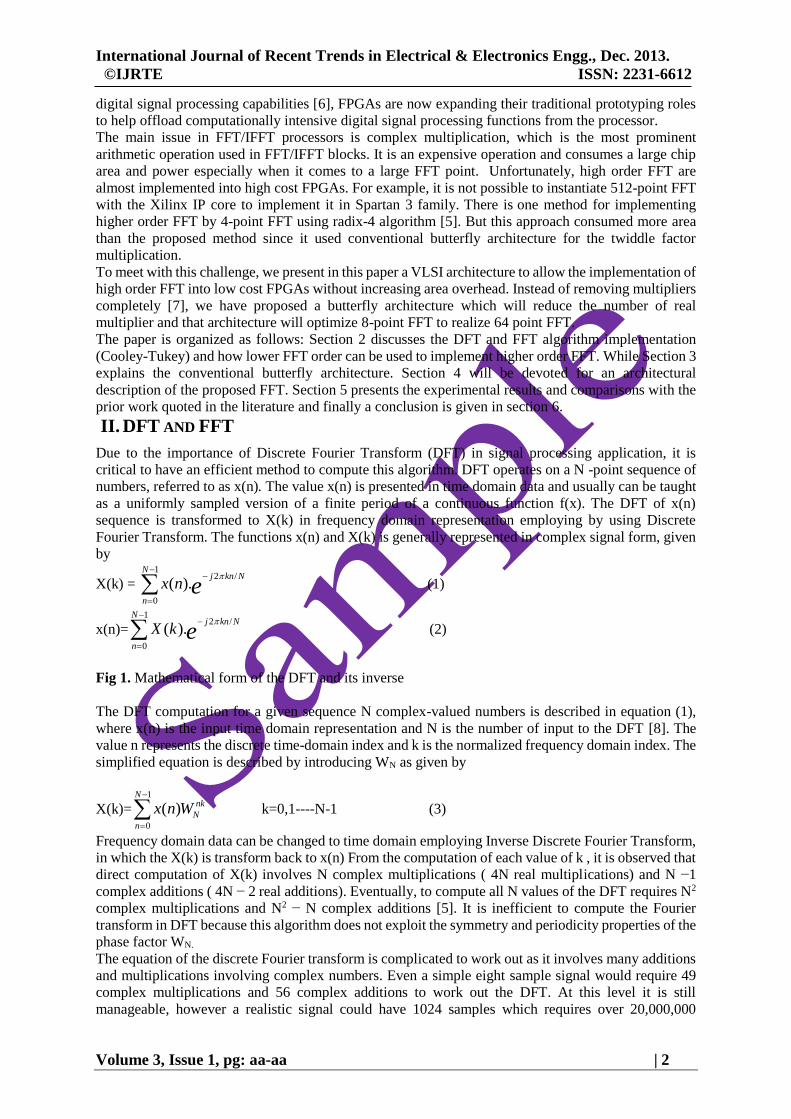
by

X(k) = 1

2 /

0

( ).N

j kn N

n

x n e

(1)

x(n)=1

2 /

0

( ).N

j kn N

n

X k e

(2)

Fig 1. Mathematical form of the DFT and its inverse

The DFT computation for a given sequence N complex-valued numbers is described in equation (1),

where x(n) is the input time domain representation and N is the number of input to the DFT [8]. The

value n represents the discrete time-domain index and k is the normalized frequency domain index. The

simplified equation is described by introducing WN as given by

X(k)=1

0

( )N

nk

N

n

x n W

k=0,1----N-1 (3)

Frequency domain data can be changed to time domain employing Inverse Discrete Fourier Transform,

in which the X(k) is transform back to x(n) From the computation of each value of k , it is observed that

direct computation of X(k) involves N complex multiplications ( 4N real multiplications) and N −1

complex additions ( 4N − 2 real additions). Eventually, to compute all N values of the DFT requires N2

complex multiplications and N2 − N complex additions [5]. It is inefficient to compute the Fourier

transform in DFT because this algorithm does not exploit the symmetry and periodicity properties of the

phase factor WN.

The equation of the discrete Fourier transform is complicated to work out as it involves many additions

and multiplications involving complex numbers. Even a simple eight sample signal would require 49

complex multiplications and 56 complex additions to work out the DFT. At this level it is still

manageable, however a realistic signal could have 1024 samples which requires over 20,000,000




complex multiplications and additions. As we can see the number of calculations required soon mounts

up to unmanageable proportions. To make the DFT operation more practical, several FFT algorithms

were proposed. The fundamental approach for all of them is to make use of the properties of the DFT

operation itself. All of them reduce the computational cost of performing the DFT on the given input

sequence. 2 /n j kn N

NW e

This value of WN is referred to as the twiddle factor or phase factor. This value of twiddle factor being a

trigonometric function over discrete points around the 4 quadrants of the two dimensional plane has

some symmetry and periodicity properties.

Symmetry property: /2k N k

N NW W

Periodicity property: k N k

N NW W

Using these properties of twiddle factor, unnecessary computations can be eliminated. The

Cooley-Tukey FFT is the most universal of all FFT algorithms, because of any factorization of N is

possible. FFT algorithm relies on divide and conquer methodology dividing N coefficients points into

smaller blocks of different sizes. The first stage computes with groups of two coefficients, yielding N/2

blocks, each computing the addition and subtraction of the coefficients scaled by the corresponding

twiddle factors, called a butterfly for its cross-over appearance [9]. These results are used to compute

the next state of N/4 blocks, which will then combine the results of two previous blocks, combining 4

coefficients at this point. This process is repeated until we have one main block, with a final

computation of all N coefficients.

The computation of the N point DFT via the decimation-in-frequency FFT, as in the decimation-in-time

algorithm requires (N/2)log2N complex multiplication and N.log2N complex addition . Let us consider

N=M.T, N=DFT length, k=s+T.t and n=l+M.n, where M and N are integers and s, l {0,1….M-1} and

t,m{ 0,1…..T-1} applying these considerations in equation (3) we will obtain

X(s+T.t) = 1 1

( )( )

0 0

[ ( . ) ]M T

l Mm s Tt

MT

l m

x l M m W

(4)

Finally we can write the equation as the following

X(s+T.t) = 1 1

( )( )

.

0 0

[ ( ) ]M T

l Mm s Tt

M T

l m

x l Mm W

(5)

It is clear from the above equation that n order to realize N point FFT , it is possible to first decompose

it into one M point and one T point FFT where N=M.T and then combining them finally. We can take

the example of 64 point to perform 64 point FFT we can go for M=T=8. Then using equation (5)

X(s+T.t)=1 1

. . .

.

0 0

[ ( ) ]M T

l t l s m s

M M T T

l m

W W x l Mm W

(6)

Equation (6) represents two dimensional structure of 8 point FFT representing 64 point FFT. Hence

performance of 64 point FFT will now depend upon 8 point performance.

By adopting divide and conquer approach, a computationally efficient algorithm for the DFT can be

developed. This approach depends on the decomposition of an N-point DFT into successively smaller

size DFTs. If N is factored as N=r1 r2 r3 r4…..rL where r1=r2=r3=….=rL, then N=rL. Hence the DFT will

be of size ‘r’, where this number ‘r’ is called the radix of the FFT algorithm. Radix-2 is the most widely

used FFT algorithm.The basic 2-point DFT performed in the radix-2 decimation-in-time algorithm. The

algorithm consists of three main steps:

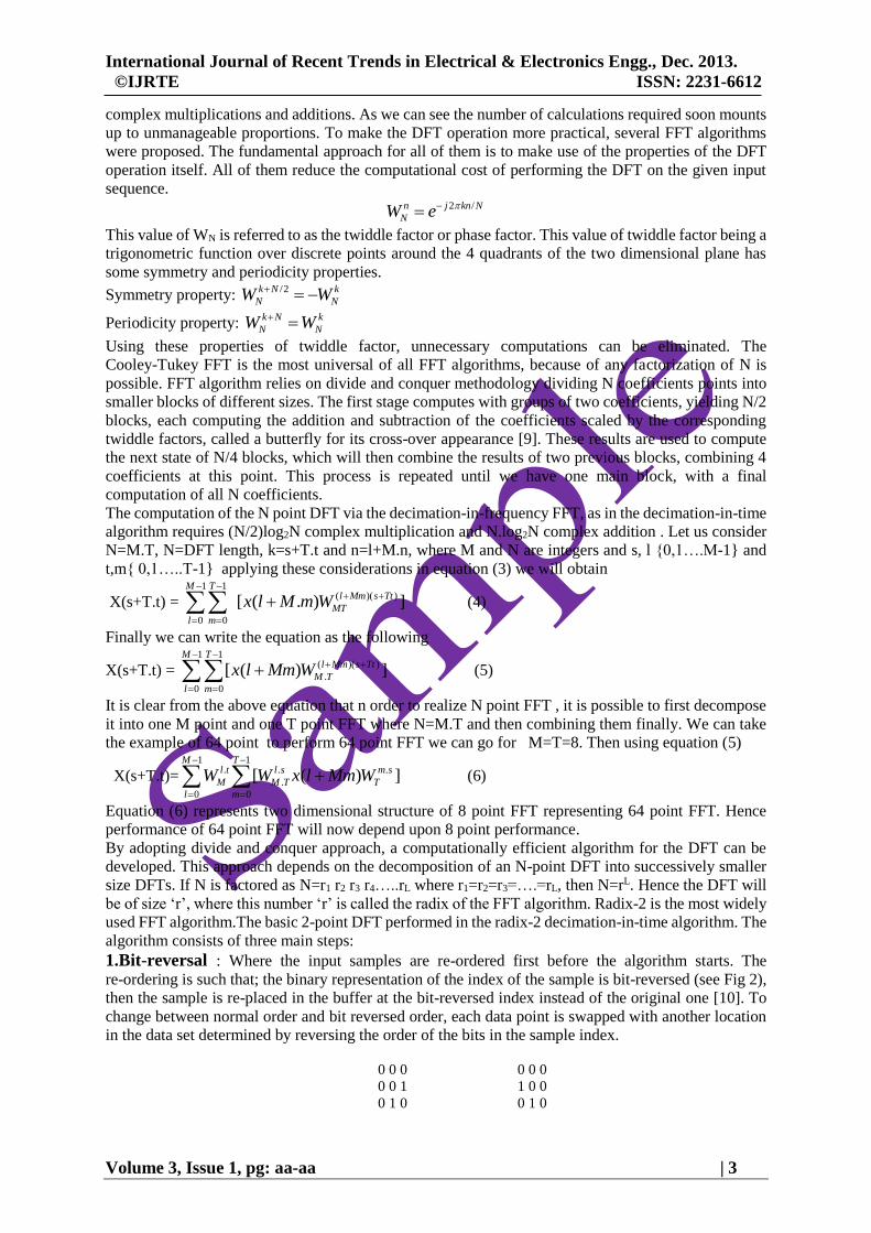
1.Bit-reversal : Where the input samples are re-ordered first before the algorithm starts. The

re-ordering is such that; the binary representation of the index of the sample is bit-reversed (see Fig 2),

then the sample is re-placed in the buffer at the bit-reversed index instead of the original one [10]. To

change between normal order and bit reversed order, each data point is swapped with another location

in the data set determined by reversing the order of the bits in the sample index.

0 0 0 0 0 0

0 0 1 1 0 0

0 1 0 0 1 0




0 1 1 1 1 0

1 0 0 0 0 1

1 0 1 1 0 1

1 1 0 0 1 1

1 1 1 1 1 1

Fig 2. Bit Reversal for 3 Bits Index

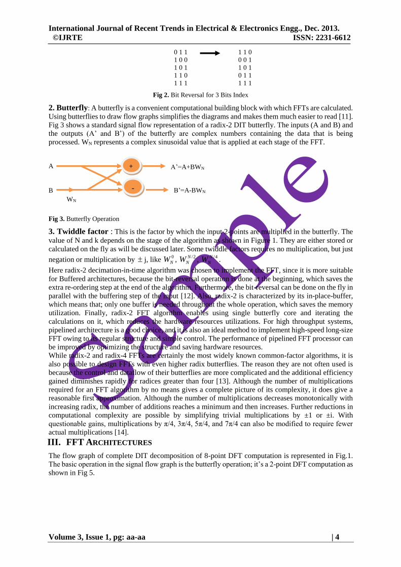
2. Butterfly: A butterfly is a convenient computational building block with which FFTs are calculated.

Using butterflies to draw flow graphs simplifies the diagrams and makes them much easier to read [11].

Fig 3 shows a standard signal flow representation of a radix-2 DIT butterfly. The inputs (A and B) and

the outputs (A’ and B’) of the butterfly are complex numbers containing the data that is being

processed. WN represents a complex sinusoidal value that is applied at each stage of the FFT.

A

B

Fig 3. Butterfly Operation

3. Twiddle factor : This is the factor by which the input 2-points are multiplied in the butterfly. The

value of N and k depends on the stage of the algorithm as shown in Figure 1. They are either stored or

calculated on the fly as will be discussed later. Some twiddle factors requires no multiplication, but just

negation or multiplication by j, like 0

NW , /2N

NW , /4N

NW .

Here radix-2 decimation-in-time algorithm was chosen to implement the FFT, since it is more suitable

for Buffered architectures, because the bit-reversal operation is done at the beginning, which saves the

extra re-ordering step at the end of the algorithm. Furthermore, the bit-reversal can be done on the fly in

parallel with the buffering step of the input [12]. Also, radix-2 is characterized by its in-place-buffer,

which means that; only one buffer is needed throughout the whole operation, which saves the memory

utilization. Finally, radix-2 FFT algorithm enables using single butterfly core and iterating the

calculations on it, which reduces the hardware resources utilizations. For high throughput systems,

pipelined architecture is a good choice, and it is also an ideal method to implement high-speed long-size

FFT owing to its regular structure and simple control. The performance of pipelined FFT processor can

be improved by optimizing the structure and saving hardware resources.

While radix-2 and radix-4 FFTs are certainly the most widely known common-factor algorithms, it is

also possible to design FFTs with even higher radix butterflies. The reason they are not often used is

because the control and dataflow of their butterflies are more complicated and the additional efficiency

gained diminishes rapidly for radices greater than four [13]. Although the number of multiplications

required for an FFT algorithm by no means gives a complete picture of its complexity, it does give a

reasonable first approximation. Although the number of multiplications decreases monotonically with

increasing radix, the number of additions reaches a minimum and then increases. Further reductions in

computational complexity are possible by simplifying trivial multiplications by ±1 or ±i. With

questionable gains, multiplications by π/4, 3π/4, 5π/4, and 7π/4 can also be modified to require fewer

actual multiplications [14].

III. FFT ARCHITECTURES

The flow graph of complete DIT decomposition of 8-point DFT computation is represented in Fig.1.

The basic operation in the signal flow graph is the butterfly operation; it’s a 2-point DFT computation as

shown in Fig 5.

WN +

+

-

+ A’=A+BWN

B’=A-BWN




Fig 4 .Three stages in the computation of 8-point DFT

The whole FFT processor architecture consists of butterfly unit, data storage unit and address generator

unit [15]. The butterfly operation is the heart of the FFT algorithm, which can influence system speed,

power consumption and cost. As shown in Fig 4, the basic butterfly unit in Fig 5, constitutes the

computation structure of the complete flow graph of radix-2 8-point FFT, in which a 2-point DFT can

be performed [16],[17]. The conventional radix-2 DIT butterfly architecture is consisting of complex

data I/O, complex multiplier and finally complex adder and subtractor Fig. 2. Consider A and B are the

complex input data, the complex twiddle factor considered as W = Wr - jWi. Finally the complex output

are X and Y . The index r and i represent the real and imaginary parts respectively.

X = A + BW

Y = A – BW

(Xr +j Xi) = (Ar +j Ai) + [ ( Wr + j Wi ) x (Br +j Bi) ] (7)

(Yr +j Yi) = (Ar +j Ai) - [ (Wr + j Wi) x (Br +j Bi) ] (8)

Fig 5. Radix-2 DIT FFT Butterfly Architecture

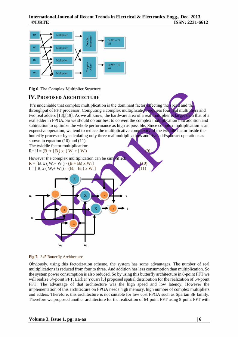
The implementation of the complex multiplier required four real multipliers and two real adders Fig 6.

(Br + jBi) X (Wr + jWi) = (Br xWr)-(Bi xWi)]+j[(Br x jWi)+ (jBi x Wr)]

The real and imaginary parts of the multiplication result is [(Br xWr)-(Bi x Wi)] and [(Br x jWz)+( jBi x

Wr)] respectively.

Ar Delay Unit

Delay Unit Ai

Br

Bi

Complex

Multiplier

Wr Wi

C

om

ple

x

Ad

der

C

om

ple

x

Su

btr

acto

r

Xr

Xi

Yr

Yi

2-point

DFT

Combine

2-point

DFTs

C

om

bin

e 4

-poin

t D

FT

s

2-point

DFT

2-point

DFT

2-point

DFT

Combine

2-point

DFTs

X[0]

X[1]

X[2]

X[3]

X[4]

X[5]

X[6]

X[7]

X[0]

X[4]

X[2]

X[6]

X[1]

X[5]

X[3]

X[7]




Fig 6. The Complex Multiplier Structure

IV. PROPOSED ARCHITECTURE

It’s undeniable that complex multiplication is the dominant factor affecting the speed and the

throughput of FFT processor. Computing a complex multiplication requires four real multipliers and

two real adders [18],[19]. As we all know, the hardware area of a real multiplier is larger than that of a

real adder in FPGA. So we should do our best to convert the complex multiplication into addition and

subtraction to optimize the whole performance as high as possible. Since complex multiplication is an

expensive operation, we tend to reduce the multiplicative complexity of the twiddle factor inside the

butterfly processor by calculating only three real multiplications and five add/subtract operations as

shown in equation (10) and (11).

The twiddle factor multiplication:

R+ jI = (Br + j B

i) x ( W

r + j W

i) (9)

However the complex multiplication can be simplified:

R = [Br x ( Wr+ Wi ) - (Br+ Bi) x Wi ] (10)

I = [ Br x ( Wr+ Wi ) - (Br – Bi ) x Wr ] (11)

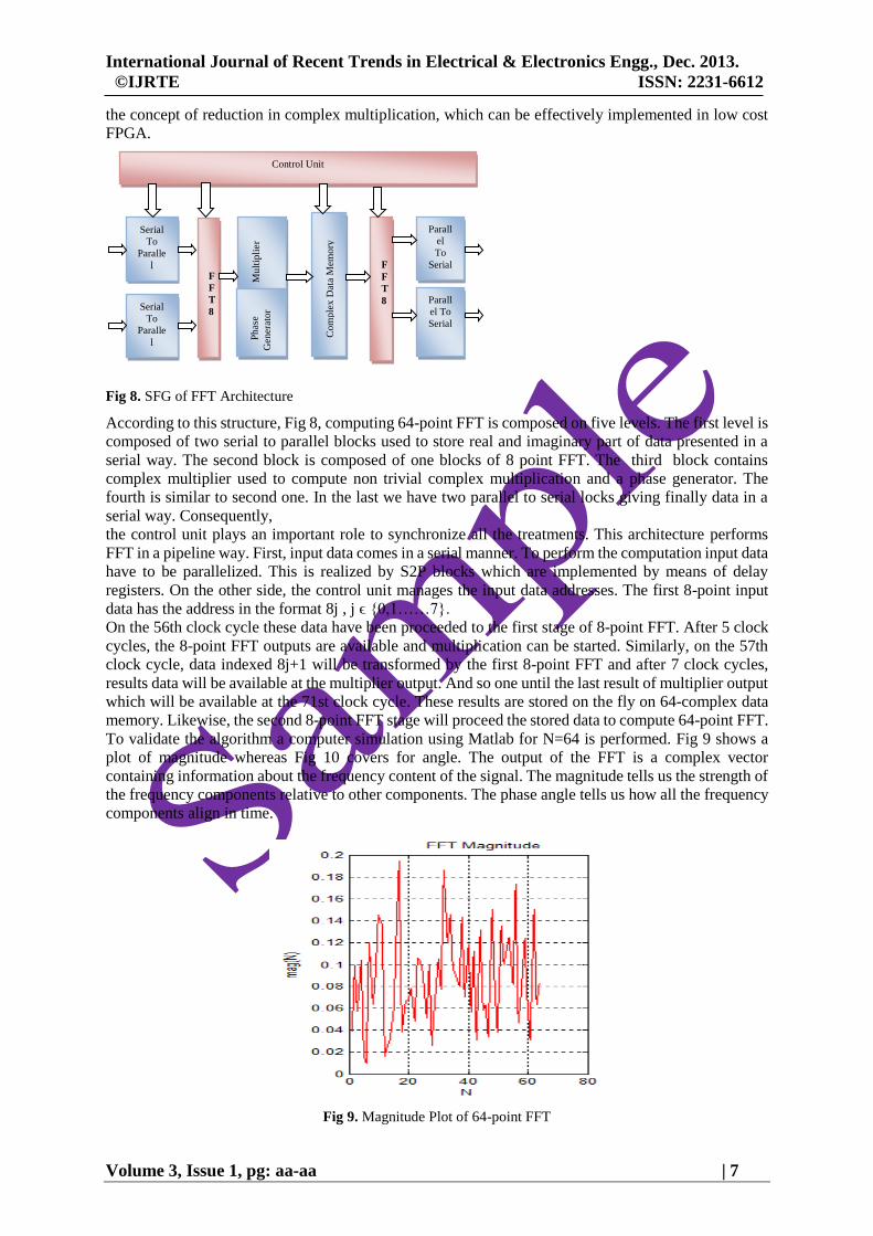
Fig 7. 3x5 Butterfly Architecture

Obviously, using this factorization scheme, the system has some advantages. The number of real

multiplications is reduced from four to three. And addition has less consumption than multiplication. So

the system power consumption is also reduced. So by using this butterfly architecture in 8-point FFT we

will realize 64-point FFT. Earlier Yousri [5] proposed spatial distribution for the realization of 64-point

FFT. The advantage of that architecture was the high speed and low latency. However the

implementation of this architecture on FPGA needs high memory, high number of complex multipliers

and adders. Therefore, this architecture is not suitable for low cost FPGA such as Spartan 3E family.

Therefore we proposed another architecture for the realization of 64-point FFT using 8-point FFT with

Multiplier

Multiplier

Multiplier

Multiplier

Br

W

r

Bi

Wi

Com

ple

x

Subtr

acto

r

Com

ple

x

A

dder

Br Wr – Bi

Wi

Br Wr + Bi

Wi

+

+

+

+

+

X

X

X

Br

Bi

Wr Wi

R

I




the concept of reduction in complex multiplication, which can be effectively implemented in low cost

FPGA.

Fig 8. SFG of FFT Architecture

According to this structure, Fig 8, computing 64-point FFT is composed on five levels. The first level is

composed of two serial to parallel blocks used to store real and imaginary part of data presented in a

serial way. The second block is composed of one blocks of 8 point FFT. The third block contains

complex multiplier used to compute non trivial complex multiplication and a phase generator. The

fourth is similar to second one. In the last we have two parallel to serial locks giving finally data in a

serial way. Consequently,

the control unit plays an important role to synchronize all the treatments. This architecture performs

FFT in a pipeline way. First, input data comes in a serial manner. To perform the computation input data

have to be parallelized. This is realized by S2P blocks which are implemented by means of delay

registers. On the other side, the control unit manages the input data addresses. The first 8-point input

data has the address in the format 8j , j ϵ {0,1……7}.

On the 56th clock cycle these data have been proceeded to the first stage of 8-point FFT. After 5 clock

cycles, the 8-point FFT outputs are available and multiplication can be started. Similarly, on the 57th

clock cycle, data indexed 8j+1 will be transformed by the first 8-point FFT and after 7 clock cycles,

results data will be available at the multiplier output. And so one until the last result of multiplier output

which will be available at the 71st clock cycle. These results are stored on the fly on 64-complex data

memory. Likewise, the second 8-point FFT stage will proceed the stored data to compute 64-point FFT.

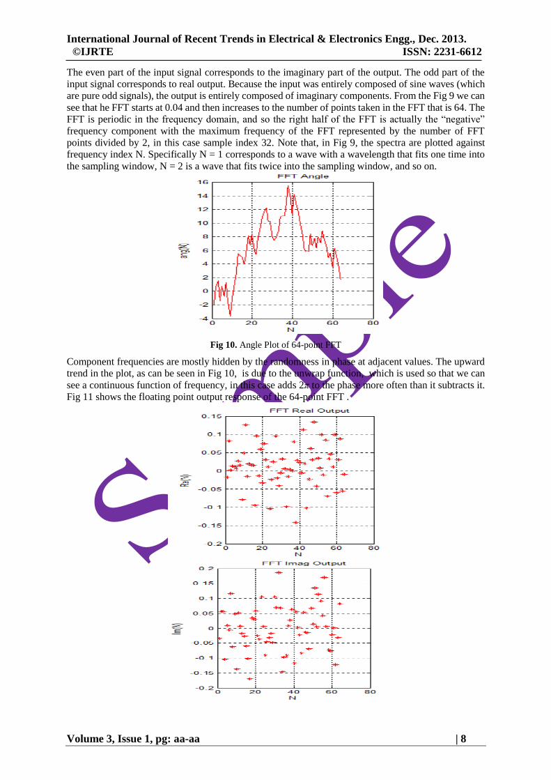
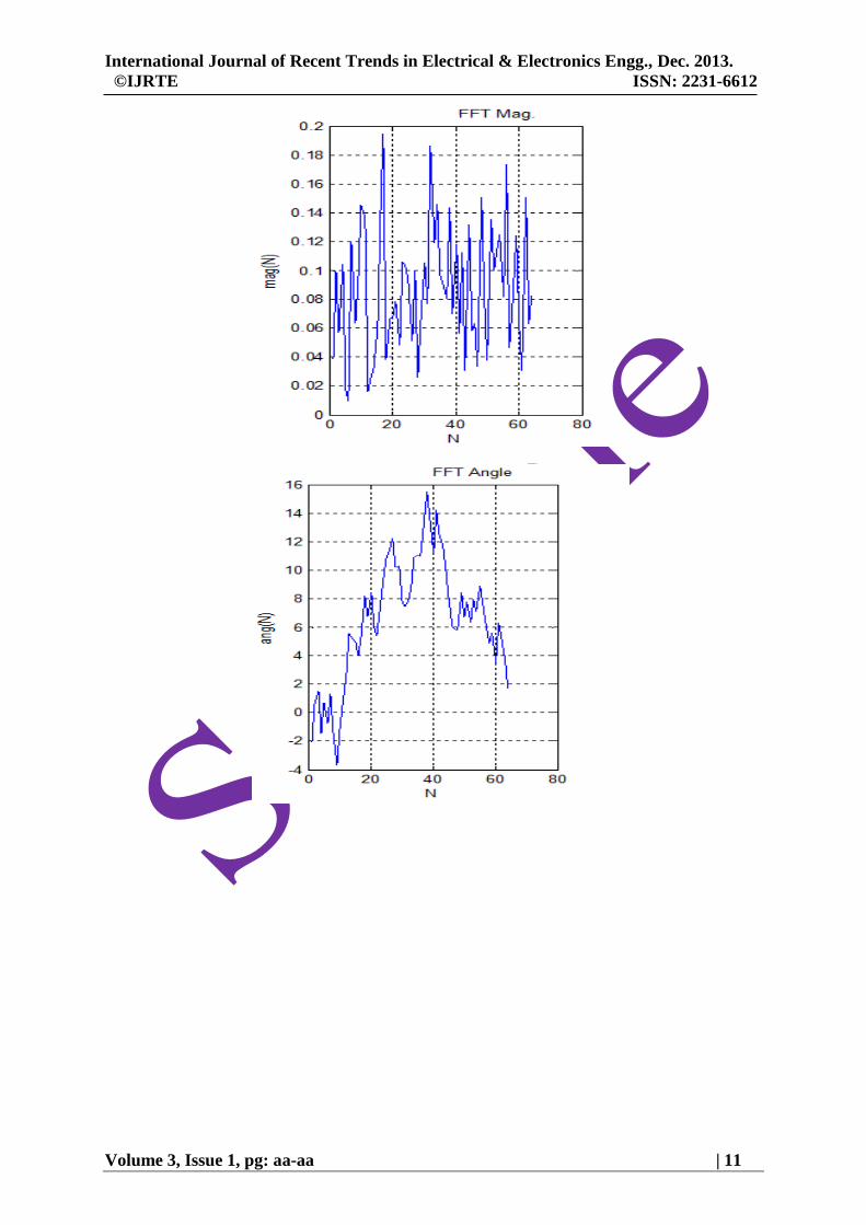
To validate the algorithm a computer simulation using Matlab for N=64 is performed. Fig 9 shows a

plot of magnitude whereas Fig 10 covers for angle. The output of the FFT is a complex vector

containing information about the frequency content of the signal. The magnitude tells us the strength of

the frequency components relative to other components. The phase angle tells us how all the frequency

components align in time.

Fig 9. Magnitude Plot of 64-point FFT

Serial

To

Paralle

l

F

F

T

8

Mult

ipli

er

P

has

e

Gen

erat

or

C

om

ple

x D

ata

Mem

ory

F

F

T

8

Control Unit

Serial

To

Paralle

l

Parall

el

To

Serial

Parall

el To

Serial




The even part of the input signal corresponds to the imaginary part of the output. The odd part of the

input signal corresponds to real output. Because the input was entirely composed of sine waves (which

are pure odd signals), the output is entirely composed of imaginary components. From the Fig 9 we can

see that he FFT starts at 0.04 and then increases to the number of points taken in the FFT that is 64. The

FFT is periodic in the frequency domain, and so the right half of the FFT is actually the “negative”

frequency component with the maximum frequency of the FFT represented by the number of FFT

points divided by 2, in this case sample index 32. Note that, in Fig 9, the spectra are plotted against

frequency index N. Specifically N = 1 corresponds to a wave with a wavelength that fits one time into

the sampling window, N = 2 is a wave that fits twice into the sampling window, and so on.

Fig 10. Angle Plot of 64-point FFT

Component frequencies are mostly hidden by the randomness in phase at adjacent values. The upward

trend in the plot, as can be seen in Fig 10, is due to the unwrap function, which is used so that we can

see a continuous function of frequency, in this case adds 2π to the phase more often than it subtracts it.

Fig 11 shows the floating point output response of the 64-point FFT .




Fig 11. Floating Point Output Response

05

1015202530354045

Slice

s

Flip Fl

ops

Multi

pliers

% Proposed Design

Design in [5]

Fig 12. Resource Utilization Comparison




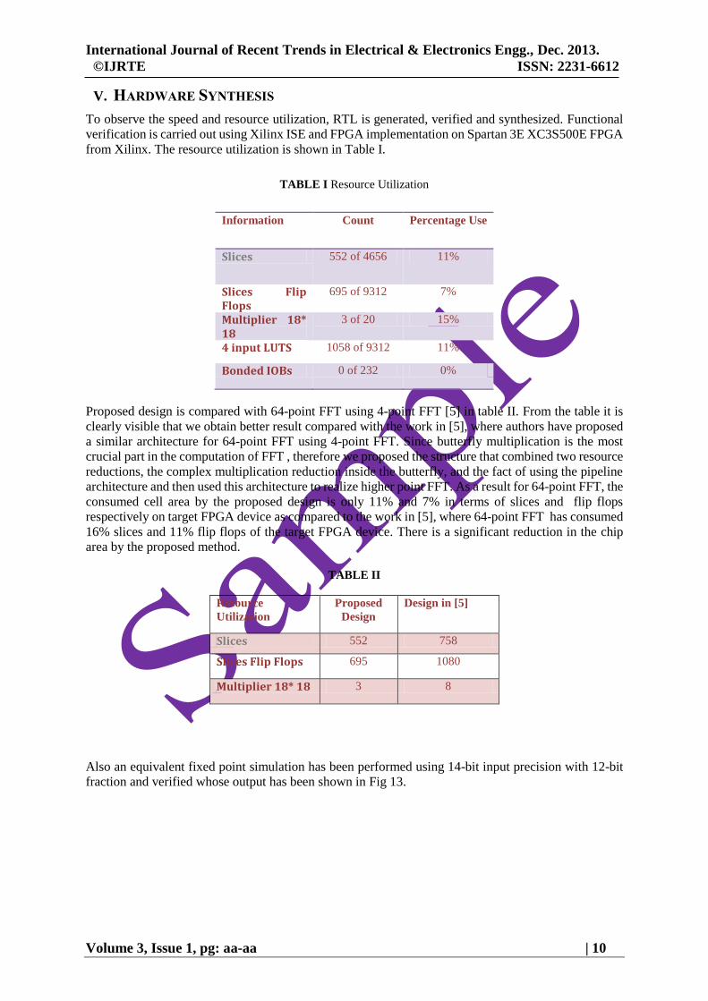
V. HARDWARE SYNTHESIS

To observe the speed and resource utilization, RTL is generated, verified and synthesized. Functional

verification is carried out using Xilinx ISE and FPGA implementation on Spartan 3E XC3S500E FPGA

from Xilinx. The resource utilization is shown in Table I.

TABLE I Resource Utilization

Information Count Percentage Use

Slices 552 of 4656 11%

Slices Flip Flops

695 of 9312 7%

Multiplier 18* 18

3 of 20 15%

4 input LUTS 1058 of 9312 11%

Bonded IOBs 0 of 232 0%

Proposed design is compared with 64-point FFT using 4-point FFT [5] in table II. From the table it is

clearly visible that we obtain better result compared with the work in [5], where authors have proposed

a similar architecture for 64-point FFT using 4-point FFT. Since butterfly multiplication is the most

crucial part in the computation of FFT , therefore we proposed the structure that combined two resource

reductions, the complex multiplication reduction inside the butterfly, and the fact of using the pipeline

architecture and then used this architecture to realize higher point FFT. As a result for 64-point FFT, the

consumed cell area by the proposed design is only 11% and 7% in terms of slices and flip flops

respectively on target FPGA device as compared to the work in [5], where 64-point FFT has consumed

16% slices and 11% flip flops of the target FPGA device. There is a significant reduction in the chip

area by the proposed method.

TABLE II

Resource

Utilization

Proposed

Design

Design in [5]

Slices 552 758

Slices Flip Flops 695 1080

Multiplier 18* 18 3 8

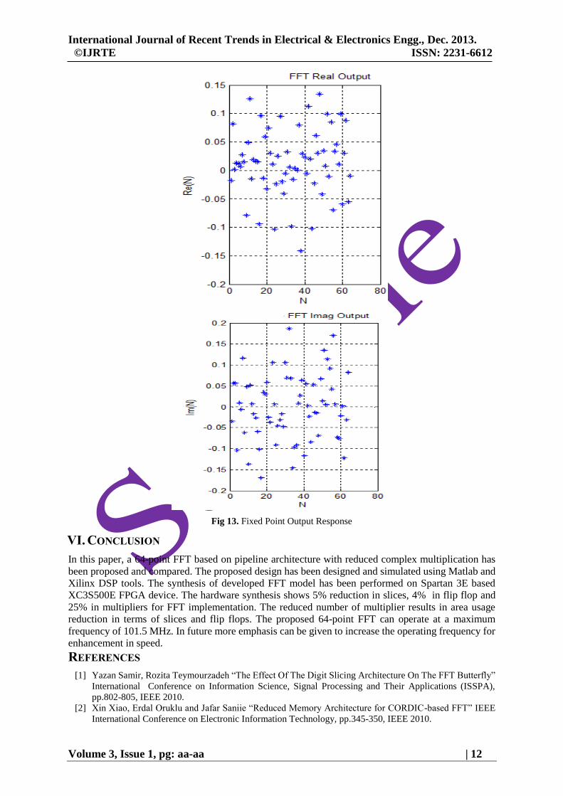
Also an equivalent fixed point simulation has been performed using 14-bit input precision with 12-bit

fraction and verified whose output has been shown in Fig 13.




Fig 13. Fixed Point Output Response

VI. CONCLUSION

In this paper, a 64-point FFT based on pipeline architecture with reduced complex multiplication has

been proposed and compared. The proposed design has been designed and simulated using Matlab and

Xilinx DSP tools. The synthesis of developed FFT model has been performed on Spartan 3E based

XC3S500E FPGA device. The hardware synthesis shows 5% reduction in slices, 4% in flip flop and

25% in multipliers for FFT implementation. The reduced number of multiplier results in area usage

reduction in terms of slices and flip flops. The proposed 64-point FFT can operate at a maximum

frequency of 101.5 MHz. In future more emphasis can be given to increase the operating frequency for

enhancement in speed.

REFERENCES

[1] Yazan Samir, Rozita Teymourzadeh “The Effect Of The Digit Slicing Architecture On The FFT Butterfly”

International Conference on Information Science, Signal Processing and Their Applications (ISSPA),

pp.802-805, IEEE 2010.

[2] Xin Xiao, Erdal Oruklu and Jafar Saniie “Reduced Memory Architecture for CORDIC-based FFT” IEEE

International Conference on Electronic Information Technology, pp.345-350, IEEE 2010.




[3] Shakeel S. Abdulla, Haewoon Nam, Mark Mc Dermot “A High Throughput FFT Processor With No

Multipliers” International Conference on Computer Design(ICCD), pp.485-495, IEEE 2009.

[4] Mao-Hsu Yen, Pao-Ann Hsiung, Sao-Jie Chen “ A Low Power 64-Point Pipeline FFT/IFFT Processor”

IEEE Transactions on Consumer Electronics, Volume No. 57, Issue No. 1, pp. 40-45, February 2011.

[5] Yousri Ouerhani, Maher Jridi “Implementation Techniques of High-Order FFT into Low-Cost FPGA”

International Midwest Symposium on Circuits and Systems (MWSCAS), pp.1-4, IEEE 2011.

[6] Ahmad A. Al Sallab, Dr. Hossam Fahmy, Prof. Dr. Mohsen Rashwan “Optimized Hardware

Implementation Of FFT Processor” International Conference on Circuits and Systems, pp.208-213, IEEE

2009.

[7] Zou Wen, Qiu Zhongpan, Song Zhijun “FPGA Implementation of efficient FFT algorithm based on

complex sequence” International Conference on Electronic Computers, pp.614-617, IEEE 2010.

[8] Muhammad Ahsan, Ehtsham Elahi, Waqas Ahmad Farooqi “Superscalar Power Efficient Fast Fourier

Transform FFT Architecture” IEEE Transaction on Computers, Volume No.24, Issue No.31, pp.414-426,

June 2011.

[9] Earl E. Swartzlander, Hani H.M. Saleh “FFT Implementation with Fused Floating-Point Operations” IEEE

Transaction On Computers, Volume No.61, Issue No.2, pp.312-317, February 2012.

[10] S. Winograd “On computing the discrete Fourier transform” Math Computation, Volume No. 32, Issue

No.1, pp. 175–199, January 2008.

[11] Bingrui Wang, Qihui Zhang, Tianyong Ao, Mingju Huang, "Design of Pipelined FFT Processor Based on

FPGA," Second International Conference on Computer Modeling and Simulation, pp.152-155, 2010.

[12] Y. Zhou, J. M. Noras and S. J. Shephend "Novel design of multiplier-less FFT processors“ IEEE

Transcation on Signal Processing, Volume No.87, Issue No.6, pp.1402-1409, June 2007.

[13] H. Sorensen, M. Heindeman, and C. Burrus “On computing the split radix FFT” IEEE Transaction on

Acoustics, Speech, Signal Process, Volume No.34, Issue No.6, pp.152-156, July 2007.

[14] Fangming Liu, Xiaozhong Pan “Research on Implementation of FFT Based on FPGA” International

Conference on Computer Application and System Modeling (ICCASM ), pp.152-155, IEEE 2010.

[15] Huan Liu, Wei Pan, Shui Sheng Lin "A New Fabric of Reconfigurable FFT Processor for High-speed and

Low-cost System" International Conference on Machine Learning and Cybernetics, pp.32-36, May 2008.

[16] N. Mahdavi, R Teymourzadeh, Masuri Bin Othman “On-Chip Implementation of High Speed and High

resolution Pipeline Radix-2 FFT Algorithm" International Conference on Intelligent and Advanced

Systems, pp.1-6, June 2007.

[17] Earl E. Swartzlander, Life Fellow “FFT Implementation with Fused Floating-Point Operations” IEEE

Transaction on Computers, Volume No.61, Issue No. 2, pp.11-19, February 2012.

[18] H. Saleh and E.E. Swartzlander “A Floating-Point Fused Add-Subtract Unit” International Midwest

Symposium on Circuits and Systems (MWSCAS), pp.519-522, IEEE 2008.

[19] Chin-Teng Lin, Yuan-Chu Yu, and Lan-Da Van “A low-power 64-point FFT-IFFT design for IEEE

802.11a WLAN application” International Symposium on Circuits and Systems (ISCAS), pp. 4523-4526,

IEEE 2006.

fpga based area efficient 64-point fft using mac … based area efficient 64-point fft using mac...

Documents