Fourier Transform in

Image Processing

Review - Image as a Function

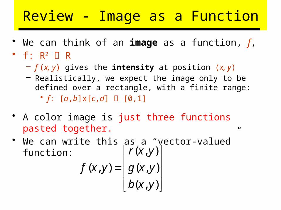
• We can think of an image as a function, f, • f: R2 R

– f (x, y) gives the intensity at position (x, y) – Realistically, we expect the image only to be defined over a

rectangle, with a finite range:• f: [a,b]x[c,d] [0,1]

• A color image is just three functions pasted together. • We can write this as a “vector-valued” function:

( , )

( , ) ( , )

( , )

r x y

f x y g x y

b x y

Image as a Function

• function, f, • f: R2 R

– f (x, y) gives the intensity at position (x, y)

Linear Transformations

on Images

Transformations on Images

• Define a new image g in terms of an existing image f– We can transform:

1. either the domain

2. or the range of f

• Range transformation:

1. What kinds of operations on the image can this transformation perform?

2. What t transformations are good for what?

1. Some operations preserve the range but change the domain of f

2. Here is an example that changes the domain :

– What kinds of operations can this perform?

3. Still other operations operate on both the domain and the range of f .

Operations that change the domain of image

1. In general we are interested in all these transformations2. Specifically we want them to have some nice (like linear)

properties

Linear Shift Invariant Systems (LSIS)

Linearity:

1f 1g 2f 2g

21 ff 21 gg

Shift invariance:

axf axg

a a

Example of LSIS: ideal lens

Defocused image ( g ) is a processed version of the focused image ( f )

g f

Ideal lens is a LSIS xf xgLSIS

Linearity: Brightness variationShift invariance: Scene movement

(this is not valid for lenses with non-linear distortions)

Linear Shift Invariant Systems (LSIS)

A Reminder of a Convolution

concept

LSIS is Doing a Convolution

convolution is linear and shift invariant

f

hfgdxhfxg

h

h

x

kernel h

Linear Shift Invariant Systems (LSIS)

1. Continuous convolution defined by integral

2. Discrete convolution from previous lectures defined by finite sumsWe negate

(mirror) the kernel of convolution h

Convolution – two more Examples

fg

gf From Eric Weinstein’s Math World

hfgdxhfxg

Here we show two more examples of convolution of functions f and g

We use two non-idea approximation of Dirac’s Delta function as a signal model

1 2-1-2

xc

-1 1

1

xb

-1 1

1 xa

bac

1

Convolution – Another Example hfgdxhfxg

Here we convolve signals a and b into convolved signal c

Convolution Kernel – Impulse Response

f gh hfg

• We ask question “What h will give us g = f ?”

Dirac Delta Function (Unit Impulse)

x2

1

0

dxxfdxxxf 0

00 fdxxf

xfdxfxg

xhdxh

Sifting property: We convolve f with Dirac Delta:

And we get this

Therefore g=f when we convolve with delta

Point Spread Function

OpticalSystemscene image

• Ideally, the optical system should be a Dirac delta function. (no distortion)

x xPSFOpticalSystem

point source point spread function

• However, optical systems are never ideal.

• Point spread function of Human Eyes PSF stands for Point Spread Function

Now we apply information from last slide to optical system

If the PSF of human eye is different (not a good approximation of delta) then we have eye troubles, related to this PSF type

Point Spread Function

normal vision myopia hyperopia

Images by Richmond Eye Associatesastigmatism

PSF stands for Point Spread Function

Tell me what your PSF is and I will tell you what is your eye problem.

Properties of Convolution

• Commutative

• Associativeabba

cbacba • Cascade system

f g1h 2h

f g21 hh

f g12 hh

Convolution operator

We used in cascading filters in previous lectures. Now we have a theoretical base

These are general properties of convolution, not related to signal representation

This is unlike matrix multiplication and Kronecker (tensor) products

• So now we know what is convolution and why it is so important.

• However signals for convolution can be represented in various ways.

• So the question is, “how to represent signals?”– 1D– 2D– 3D?

How to Represent Signals?

• Option 1: Taylor series represents any function using polynomials.

• Polynomials are not the best - unstable and not very physically meaningful. (they still have some applications)

• Easier to talk about “signals” in terms of its “frequencies”

(how fast/often signals change, etc).

Mr. Jean Baptiste Fourier and

Fourier Transform idea

Jean Baptiste Joseph Fourier (1768-1830)

• Had crazy idea (1807):• Any periodic

function can be rewritten as a weighted sum of Sines and Cosines of different frequencies.

• Don’t believe it? – Neither did Lagrange,

Laplace, Poisson and other big wigs

– Not translated into English until 1878!

• But it’s true!– called Fourier Series– Possibly the greatest tool

used in Engineering

A Sum of Sinusoids

• Our building block:

• Add enough of them to get any signal f(x) you want!

• How many degrees of freedom?

• What does each control?

• Which one encodes the coarse vs. fine structure of the signal?

xAsin(

Math Review - Complex numbers

• Real numbers:1-5.2

• Complex numbers4.2 + 3.7i9.4447 – 6.7i-5.2 (-5.2 + 0i)

1i

We often denote in EE i by j

Math Review - Complex numbers

• Complex numbers4.2 + 3.7i9.4447 – 6.7i-5.2 (-5.2 + 0i)

• General FormZ = a + biRe(Z) = a

Im(Z) = b

• AmplitudeA = | Z | = √(a2 + b2)

• Phase = Z = tan-1(b/a)

Real and imaginary parts

Math Review – Complex Numbers

• Polar CoordinateZ = a + bi

• AmplitudeA = √(a2 + b2)

• Phase = tan-1(b/a)

a

b

A

Math Review – Complex Numbers and Cosine Waves

• Cosine wave has three properties– Frequency– Amplitude– Phase

• Complex number has two properties– Amplitude– Wave

• Complex numbers to represent cosine waves at varying frequency– Frequency 1: Z1 = 5 +2i– Frequency 2: Z2 = -3 + 4i– Frequency 3: Z3 = 1.3 – 1.6i

Simple but great idea !!

Fourier Transform Idea

• We want to understand the frequency w of our signal. So, let’s reparameterize the signal by w instead of x:

xAsin(

f(x) F(w)Fourier Transform

F(w) f(x)Inverse Fourier Transform

• For every w from 0 to infinity, F(w) holds the amplitude A and phase f of the corresponding sine

– How can F hold both? Complex number trick!

)()()( iIRF

22 )()( IRA )(

)(tan 1

R

I

All info preserved

Math Review - Periodic

Functions – more illustrations to our formalism

Math Review - Periodic Functions

If there is some a, for a function f(x), such that

f(x) = f(x + na)

then function is periodic with the period a

0

a 2a 3a

Math Review - Attributes of cosine wave

Amplitude

Phase

f(x) = cos (x)

f(x) = 5 cos (x)

f(x) = 5 cos (x + 3.14)

-5

-4

-3

-2

-1

0

1

2

3

4

5

-10 -5 0 5 10

-5

-3

-1

1

3

5

-10 -5 0 5 10

-5

-3

-1

1

3

5

-10 -5 0 5 10

-5

-3

-1

1

3

5

-10 -5 0 5 10

-5

-4

-3

-2

-1

0

1

2

3

4

5

-10 -5 0 5 10

Math Review - Attributes of cosine wave

Amplitude

Phase

Frequency

f(x) = 5 cos (x)

f(x) = 5 cos (x + 3.14)

f(x) = 5 cos (3 x + 3.14) -5

-3

-1

1

3

5

-10 -5 0 5 10

Math Review - Attributes of cosine wave

f(x) = cos (x)

Amplitude, Frequency, Phase

-5

-3

-1

1

3

5

-10 -5 0 5 10

f(x) = A cos (kx + )

This math is base of Fourier Analysis and Fourier Synthesis

Time and Frequency• example : g(t) = sin(2 f t) + (1/3)sin(2(3f) t)

Before we go to using complex numbers and formulas let us get intuition about time and frequency

Our periodic signal is a mixture of two frequencies

Time and Frequency

• example : g(t) = sin(2 f t) + (1/3)sin(2(3f) t)

= +

Frequency Spectra• example : g(t) = sin(2pf t) + (1/3)sin(2p(3f)

t)

= +

In time domain

In frequency domain

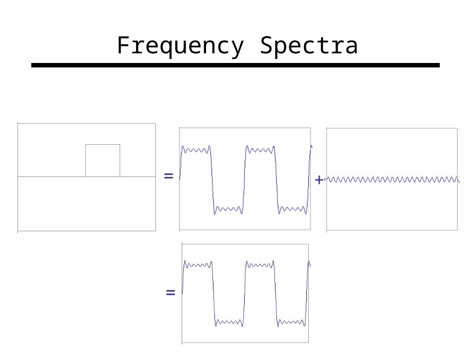
Frequency Spectra

• Usually, frequency is more interesting than the phase

1. We will decompose it to frequencies, 2. we will add one more coefficient based base

function in each slide

= +

=

Frequency Spectra

First base function second base function

Sum of first and second base functions is already not bad approximation

= +

=

Frequency Spectra

Sum of first , second and third base functions is even better approximation

= +

=

Frequency Spectra

= +

=

Frequency Spectra

= +

=

Frequency Spectra

= 1

1sin(2 )

k

A ktk

Frequency Spectra

In time domain

In frequency domain

Frequency Spectra

Observe the negative values of domain that appear in spectrum

Fourier Transform is

Just a change of basis

Important concept

Fourier Transform is Just a change of basis

.

.

.

* =

M * f(x) = F(w) M can be a matrix, a decision diagram, a butterfly, a system (physical or simulated)

IFT: Just a change of basis

.

.

.

* =

M-1 * F(w) = f(x)Inverse Fourier Transform is similarly only a change of basis

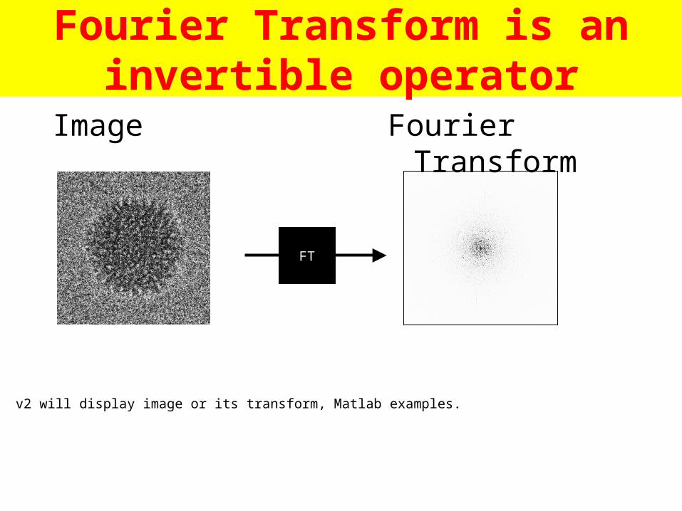
Fourier Transform is an invertible operator

Image Fourier Transform

v2 will display image or its transform, Matlab examples.

FT

Fourier Transform is an invertible operator

Image

f(x,y)F(kx,ky)

x

y

0 Nx

Ny

{F(kx,ky)} = f(x,y)} {f(x,y)} = F(kx,ky)

Nx ⁄ 2

Ny ⁄ 2Fourier Transform

Similarly as for Hadamard-Walsh or Reed-Muller Transforms we can talk about transform pairs.

Continuous Fourier

Transform

Continuous Fourier Transform

dsesFxf

dxexfsF

xsi

xsi

2

2

)()(

)()(

dsesFxf

dxexfsF

ixs

ixs

)(2

1)(

)()(

dsesFxf

dxexfsF

ixs

ixs

)(2

1)(

)(2

1)(

f(x) = F(s)

Euler’s Formula

Various normalizations of pairs

Some Conventions for Fourier Transforms

• Image Domain

• Forward Transform

• f(x,y,z)• g(x)• F

• Fourier Domain– Reciprocal space– Fourier Space– K-space– Frequency Space– Spectral domain

• Reverse Transform, Inverse Transform

• F(kx,ky,kz)• G(s)• F

Fourier Analysis

Decompose f(x) into a series of cosine waves that when summed reconstruct f(x)

Fourier Analysis in 1D. Audio signals

-5

-4

-3

-2

-1

0

1

2

3

4

5

0 200 400 600 800 1000 1200 1400

-5

-4

-3

-2

-1

0

1

2

3

4

5

0 200 400 600 800 1000 1200 1400

5 10 15

(Hz)

5 10 15

(Hz)

Amplitude OnlyAmplitude Only

Fourier Analysis in 1D. Audio signals

-5

-4

-3

-2

-1

0

1

2

3

4

5

0 200 400 600 800 1000 1200 1400

5 10 15

(Hz)

Your ear performs fourier analysis.

Fourier Analysis in 1D. Spectrum Analyzer.

iTunes performs fourier analysis.

1. We know it from our Hi-Fi equipment2. The same can be done with standard images or radar images or any other images, in

any number of dimensions

Fourier Synthesis

Summing cosine waves reconstructs the original function

Example: Fourier Synthesis of Boxcar Function

Boxcar function

Periodic Boxcar

Can this function be reproduced with cosine waves?

k=1. One cycle per period

A1·cos(2kx + 1)k=1

Ak·cos(2kx + k)k=1

1

k=2. Two cycles per period

A2·cos(2kx + 2)k=2

Ak·cos(2kx + k)k=1

2

k=3. Three cycles per period

A3·cos(2kx + 3)k=3

Ak·cos(2kx + k)k=1

3

Ak·cos(2kx + k)N

Fourier Synthesis. N Cycles

A3·cos(2kx + 3)k=3

k=1

Example: Fourier Synthesis of a 2D Function

An image is two dimensional data.

Intensities as a function of x,y

White pixels represent the highest intensities.

Greyscale image of iris128x128 pixels

Fourier Synthesis of a 2D Function

F(2,3)F(2,3)

1. We select coefficients, multiply them by weights and add2. We can create artificial images

Fourier Filters• Fourier Filters in 1D data (sound) change

the image by changing which frequencies of cosine waves go into the image

• Represented by 1D spectral profile

• 2D Specteral Profile is rotationally symmetrized 1D profile

Low and High Frequency Image Filters

• Low frequency terms– Close to origin in Fourier Space– Changes with great spatial extent (like ice

gradient), or particle size

• High frequency terms– Closer to edge in Fourier Space– Necessary to represent edges or high-

resolution features

Frequency-based Filters

1. Low-pass Filter (blurs) – Restricts data to low-frequency components

2. High-pass Filter (sharpens) – Restricts data to high-frequency-components

3. Band-pass Filter– Restrict data to a band of frequencies

4. Band-stop Filter– Suppress a certain band of frequencies

We will show many practical examples soon

Cutoff Low-pass FilterImage is blurred

Sharp features are lost

Ringing artifacts

0

0.1

0.2

0.3

0.4

0.5

0.6

0.7

0.8

0.9

1

0 0.2 0.4 0.6 0.8 1

Filter characteristics

Butterworth Low-pass FilterFlat in the pass-

band

Zero in the stop-band

No ringing

Gaussian Low-pass Filter

0

0.1

0.2

0.3

0.4

0.5

0.6

0.7

0.8

0.9

1

0 0.2 0.4 0.6 0.8 1

Butterworth High-pass Filter

• Note the loss of solid densities

How the filter looks in 2D

unprocessed

lowpass

highpass

bandpass

spectra

Convolution again

Our goal is now to approach the most important results of spectral processing

ConvolutionConvolution of some function f(x) with

some kernel g(x)

* =

Continuous

Discrete

x x

Convolution in 2D

x

x x

=

x

x x

=

x x

x x

x x

x x

image kernel result

Microscope Point-Spread-Function is Convolution

Point-Spread-Function

Convolution Theorem

f g = {FG}

f = FG

G

Convolution in image domainIs equivalent to multiplication in fourier domain

Can be derived from above because FG/G = F and f = F-1 (F)

Lowpass Filtering by Convolution

f g = {FG}• Camera shake

0

0.1

0.2

0.3

0.4

0.5

0.6

0.7

0.8

0.9

1

0 0.2 0.4 0.6 0.8 1

We showed examples of this using standard convolution, but it is done in modern equipment through digitally calculated FFT and IFFT

2D gaussian is example of kernel

2D gaussian as a matrix of a kernel

Lens Performs Fourier Transform

Contrast Theory

observed image

f(x) for true particle

point-spread function

envelope function

noise

obs(x) = f(x) psf(x) env(x) + n(x)

Incoherant average of transform

F2(s) CTF2(s) Env2(s) + N2(s)

Power spectrum

PS =

Gibbs Ringing

• 5 waves

• 25 waves

• 125 waves

Even with 125 waves we still have some small Gibbs Ringing

Fourier Transform

Math Properties

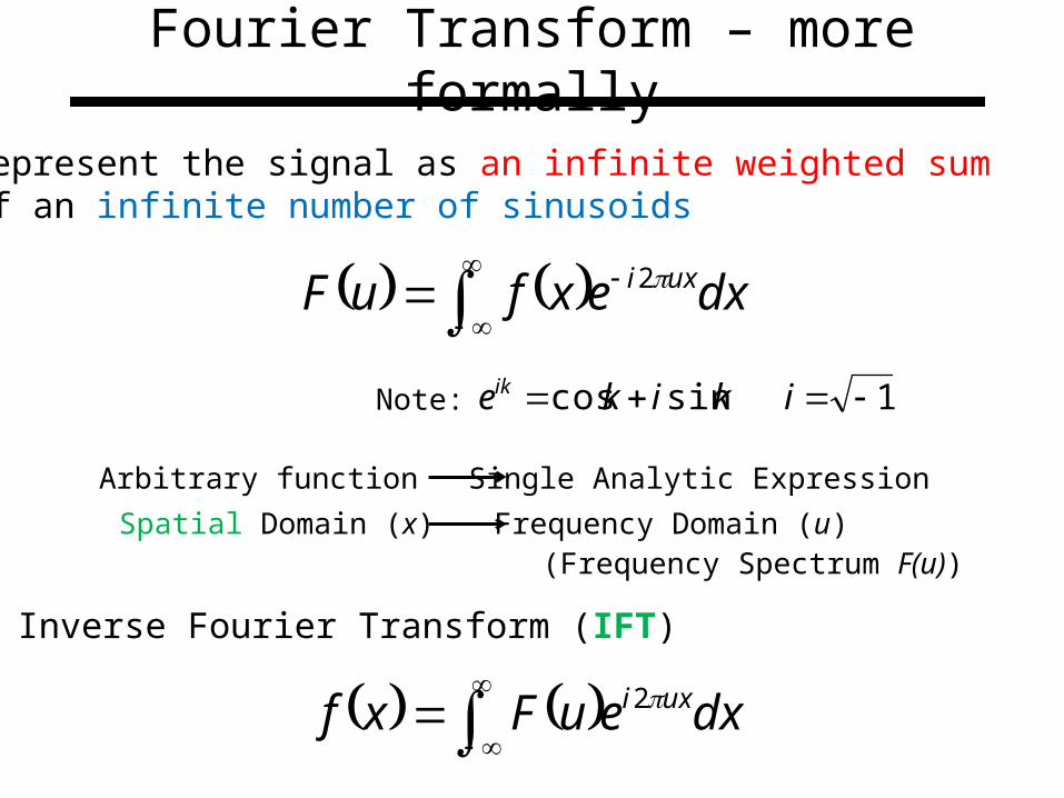
Fourier Transform – more formally

Arbitrary function Single Analytic Expression

Spatial Domain (x) Frequency Domain (u)

Represent the signal as an infinite weighted sum of an infinite number of sinusoids

dxexfuF uxi 2

(Frequency Spectrum F(u))

1sincos ikikeikNote:

Inverse Fourier Transform (IFT)

dxeuFxf uxi 2

• Also, defined as:

dxexfuF iux

1sincos ikikeikNote:

• Inverse Fourier Transform (IFT)

dxeuFxf iux

2

1

Fourier Transform

Fourier Transform

Fourier Transform

Pairs (I)

angular frequency ( )iuxeNote that these are derived using

Fourier Transform

Fourier Transform Pairs (I)

angular frequency ( )iuxeNote that these are derived using

Fourier Transform

angular frequency ( )iuxe

Note that these are derived using

Fourier Transform Pairs (I)

Fourier Transform and Convolution

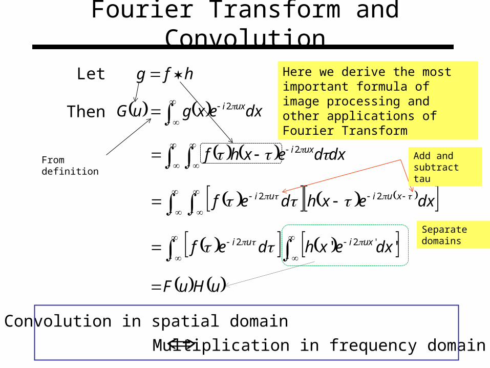
Fourier Transform and Convolution

hfg

dxexguG uxi 2

dxdexhf uxi 2

dxexhdef xuiui 22

'' '22 dxexhdef uxiui

Let

Then

uHuF

Convolution in spatial domain

Multiplication in frequency domain

Here we derive the most important formula of image processing and other applications of Fourier Transform

Add and subtract tau

From definition

Separate domains

MAIN THEOREM OF MODERN IMAGE PROCESSING:

Convolution in spatial domain

Multiplication in frequency domain

Fourier Transform and Convolution

hfg FHG fhg HFG

Spatial Domain (x) Frequency Domain (u)

So, we can find g(x) by Fourier transform

g f h

G F H

FT FTIFT

Properties of Fourier

Transform

Properties of Fourier Transform 1Spatial Domain (x) Frequency Domain (u)

Linearity xgcxfc 21 uGcuFc 21

Scaling axf

a

uF

a

1

Shifting 0xxf uFe uxi 02

Symmetry xF uf

Conjugation xf uF

Convolution xgxf uGuF

Differentiation n

n

dx

xfd uFui n2

frequency ( )uxie 2Note that these are derived using

Properties of Fourier Transform 2

Star will be used for conjugation in complex plane

1. RO – real odd2. IE – imaginary even3. IO – imaginary odd4. RE – Real even5. CE – Complex even6. CO – Complex odd

Substitute f instead of g in this formula to get the upper formula

We explained even-odd properties for Walsh, we will explain again for other transforms

For instance, when f is R then F is RE, IO,. etc

Example use of Fourier: Smoothing/Blurring

1. We want a smoothed function of f(x)

xhxfxg

H(u) attenuates high frequencies in F(u) (Low-pass Filter)!

• 3. Then

222

2

1exp uuH

uHuFuG

2

1

u

uH

2

2

2

1exp

2

1

x

xh

• 2. Let us use a Gaussian kernel

xh

x

But we do this in spectral domain

Our Images are Discrete

so discrete Fourier applies

Image as a Discrete Function

Digital Images

The scene is– projected on a 2D plane, – sampled on a regular grid, and each sample is– quantized (rounded to the nearest integer)

Image as a matrix

jifjif ,Quantize,

ReviewFourier Transform is invertible operator

Math ReviewPeriodic functions

Amplitude, Phase and Frequency

Complex numberAmplitude and Phase

Fourier Analysis (Forward Transform)Decomposition of periodic signal into cosine waves

Fourier Synthesis (Inverse Transform)Summation of cosine waves into multi-frequency waveform

Fourier Transforms in 1D, 2D, 3D, ND

Image AnalysisImage (real-valued)Transform (complex-valued,

amplitude plot)

Fourier FiltersLow-pass High-pass Band-passBand-stop

Convolution TheoremDeconvolute by Division in

Fourier Space

All Fourier Filters can be expressed as real-space Convolution Kernels

Lens does Fourier transforms Diffraction Microscopy

Where we are in this class?

• We defined continuous Fourier Transform• We defined discrete Fourier Transform DFT• DFT is calculated by matrix multiplication• It is slow• We will need factorizations, Kroneckers,

recursions and butterflies to calculate it faster.

• Only then FT will become a really useful tool, FFT.

Further Reading

• Wikipedia• Mathworld• The Fourier Transform and its

Applications. Ronald Bracewell

Filtering with EMAN2LowPass Filtersfiltered=image.process(‘filter.lowpass.guass’, {‘sigma’:0.10})

filtered=image.process(‘filter.lowpass.butterworth’, {‘low_cutoff_frequency’:0.10, ‘high_cutoff_frequency’:0.35})

filtered=image.process(‘filter.lowpass.tanh’, {‘cutoff_frequency’:0.10, ‘falloff’:0.2})

HighPass Filtersfiltered=image.process(‘filter.highpass.guass’, {‘sigma’:0.10})

filtered=image.process(‘filter.highpass.butterworth’, {‘low_cutoff_frequency’:0.10, ‘high_cutoff_frequency’:0.35})

filtered=image.process(‘filter.highpass.tanh’, {‘cutoff_frequency’:0.10, ‘falloff’:0.2})

BandPass Filtersfiltered=image.process(‘filter.bandpass.guass’, {‘center’:0.2,‘sigma’:0.10})

filtered=image.process(‘filter.bandpass.butterworth’, {‘low_cutoff_frequency’:0.10, ‘high_cutoff_frequency’:0.35})

filtered=image.process(‘filter.bandpass.tanh’, {‘cutoff_frequency’:0.10, ‘falloff’:0.2})

1. S. Narasimhan

2. Mike Marsh

National Center for Macromolecular Imaging

Baylor College of Medicine

Sources of slides