four interesting problems concerning markovian shape sequences

Four Interesting Problems concerning Markovian Shape SequencesAuthor(s): Richard Cowan and Francis K. C. ChenSource: Advances in Applied Probability, Vol. 31, No. 4 (Dec., 1999), pp. 954-968Published by: Applied Probability TrustStable URL: http://www.jstor.org/stable/1428336 .

Accessed: 18/06/2014 19:22

Your use of the JSTOR archive indicates your acceptance of the Terms & Conditions of Use, available at .http://www.jstor.org/page/info/about/policies/terms.jsp

.JSTOR is a not-for-profit service that helps scholars, researchers, and students discover, use, and build upon a wide range ofcontent in a trusted digital archive. We use information technology and tools to increase productivity and facilitate new formsof scholarship. For more information about JSTOR, please contact [email protected].

.

Applied Probability Trust is collaborating with JSTOR to digitize, preserve and extend access to Advances inApplied Probability.

http://www.jstor.org

This content downloaded from 195.34.79.208 on Wed, 18 Jun 2014 19:22:48 PMAll use subject to JSTOR Terms and Conditions

http://www.jstor.org/action/showPublisher?publisherCode=apt

http://www.jstor.org/stable/1428336?origin=JSTOR-pdf

http://www.jstor.org/page/info/about/policies/terms.jsp


Adv. Appl. Prob. (SGSA) 31, 954-968 (1999) Printed in Northern Ireland

@ Applied Probability Trust 1999

FOUR INTERESTING PROBLEMS CONCERNING MARKOVIAN SHAPE SEQUENCES

RICHARD COWAN,* University of Sydney FRANCIS K. C. CHEN,** University of Hong Kong

Abstract

In earlier work, we investigated the dynamics of shape when rectangles are split into two. Further exploration, into the more general issues of Markovian sequences of rectangular shapes, has identified four particularly appealing problems. These problems, which lead to interesting invariant distributions on [0,1], have motivating links with the classical works of Blaschke, Crofton, D. G. Kendall, Renyi and Sulanke.

Keywords: Invariant distributions; shape; stochastic geometry; distribution theory; Markov processes; dynamical systems; Brownian motion.

AMS 1991 Subject Classification: Primary 60D05 Secondary 60E05; 60J05

1. Introduction

In an earlier paper, [2], we have explored Markovian sequences of rectangular shapes. The transition rules in that paper used the device of randomly splitting a given rectangle into two sub-rectangles and selecting one of these as the next in sequence. Interesting invariant distributions arose in that context. Some of those results were also presented in a higher- dimensional setting in [3].

Shape of a rectangle in IR2 is defined for our purposes as the ratio of the shorter to longer side-lengths and so the distributions of shape have support [0, 1]. In [2], all invariant distributions had densities over this range.

We have made an extensive study of invariant distributions for other transition rules which create Markovian shape sequences of rectangles. In the course of this study, four problems have appealed to us greatly. These problems, which we now describe, arise from natural geometric constructions and lead to interesting invariant distributions. Each problem has a motivating link with classical work, so we name the problems accordingly.

Our work also has a general affinity with the studies on Markovian shape sequences for triangles, as in [6, 7].

2. Reminiscent of Renyi and Sulanke

Suppose at stage t, we have a rectangle Rt. If k independent and uniformly distributed points are placed in the interior of Rt, one might ask how these points could define a new rectangle, Rt+l. A natural method is one where Rt+l is the rectangle of smallest area having

Received 1 September 1998. * Postal address: School of Mathematics and Statistics, University of Sydney, NSW 2006, Australia. Email address: [email protected] ** Postal address: Department of Statistics, University of Hong Kong, Pokfulam Road, Hong Kong.

954



Markovian shape sequences SGSA * 955

?-----------------r-----------

....___----------------_- -172 ---,

(a) (b) (c) (d)------------------------------- (b) ~(C) d

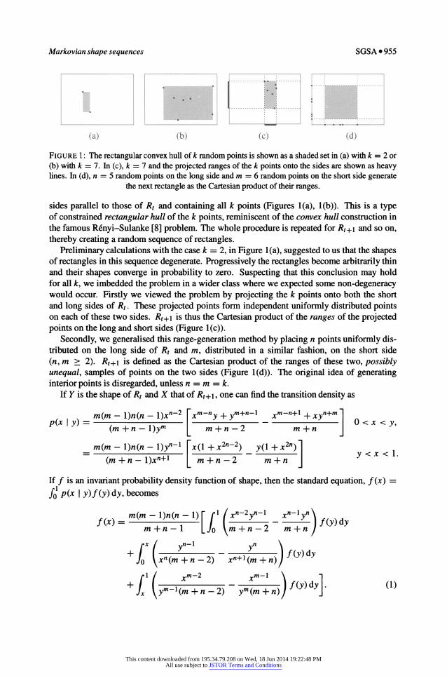
FIGURE 1: The rectangular convex hull of k random points is shown as a shaded set in (a) with k = 2 or (b) with k = 7. In (c), k = 7 and the projected ranges of the k points onto the sides are shown as heavy lines. In (d), n = 5 random points on the long side and m = 6 random points on the short side generate

the next rectangle as the Cartesian product of their ranges.

sides parallel to those of Rt and containing all k points (Figures l(a), l(b)). This is a type of constrained rectangular hull of the k points, reminiscent of the convex hull construction in the famous R6nyi-Sulanke [8] problem. The whole procedure is repeated for Rt+1 and so on, thereby creating a random sequence of rectangles.

Preliminary calculations with the case k = 2, in Figure 1(a), suggested to us that the shapes of rectangles in this sequence degenerate. Progressively the rectangles become arbitrarily thin and their shapes converge in probability to zero. Suspecting that this conclusion may hold for all k, we imbedded the problem in a wider class where we expected some non-degeneracy would occur. Firstly we viewed the problem by projecting the k points onto both the short and long sides of Rt. These projected points form independent uniformly distributed points on each of these two sides. Rt+1 is thus the Cartesian product of the ranges of the projected points on the long and short sides (Figure 1(c)).

Secondly, we generalised this range-generation method by placing n points uniformly distributed on the long side of Rt and m, distributed in a similar fashion, on the short side (n, m > 2). Rt+1 is defined as the Cartesian product of the ranges of these two, possibly unequal, samples of points on the two sides (Figure 1(d)). The original idea of generating interior points is disregarded, unless n = m = k.

If Y is the shape of Rt and X that of Rt+l, one can find the transition density as

m(m - 1)n(n - 1)xn-2 rxm-ny + ym+n-1 xm-n+l + xyn+m p(x y)=- <x<y, p(x I Y) (m +n - 1)ym m+n -2 m +n

m(m - 1)n(n - 1)yn-1 x(1 + x2n-2) y(1 + x2n) (m + n - 1)xn+l m + n - 2 m + n

If f is an invariant probability density function of shape, then the standard equation, f(x) =

fo p(x I y) f (y) dy, becomes

f(x) m(m - 1)n(n - 1) (xn-2 n- xn- f() dy

m+n-1 m+n-2 m+nf+)d

X yn- yn (y) dy +f

xn(m + n - 2)

xn+1 (m + n))

S (

m-2

xm-1 )

+ ym-l(m + n - 2) ym(m+n ) d (1)+)



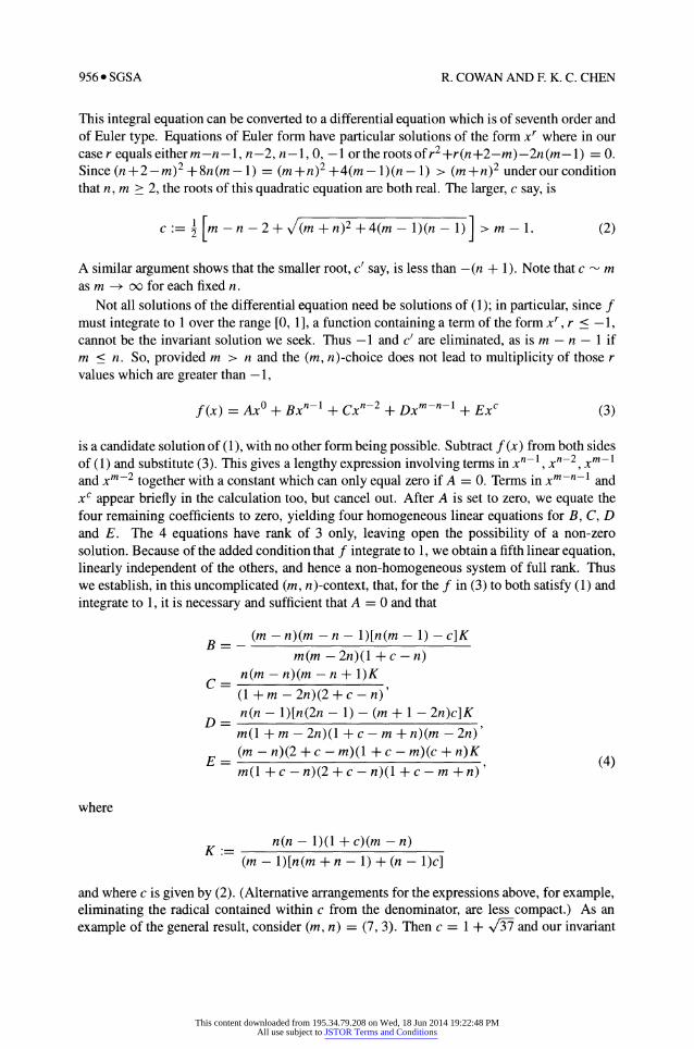
956 e SGSA R. COWAN AND F K. C. CHEN

This integral equation can be converted to a differential equation which is of seventh order and of Euler type. Equations of Euler form have particular solutions of the form xr where in our case r equals either m-n- 1, n-2, n- 1, 0, -1 I or the roots of r2+r(n+2-m)-2n(m- 1) = 0. Since (n+2-m)2 +8n(m- 1) = (m+n)2 +4(m- 1)(n- 1) > (m+n)2 underour condition that n, m > 2, the roots of this quadratic equation are both real. The larger, c say, is

c:= - n - 2 + (m n)2 +4 (m- 1)(n- 1)> m-1. (2)

A similar argument shows that the smaller root, c' say, is less than -(n + 1). Note that c - m as m -- oo for each fixed n.

Not all solutions of the differential equation need be solutions of (1); in particular, since f must integrate to 1 over the range [0, 1], a function containing a term of the form xr, r < -1, cannot be the invariant solution we seek. Thus -1 and c' are eliminated, as is m - n - 1 if m < n. So, provided m > n and the (m, n)-choice does not lead to multiplicity of those r values which are greater than -1,

f(x) = Axo + Bxn-1 + Cxn-2 + Dxm-n-1 + Exc (3)

is a candidate solution of (1), with no other form being possible. Subtract f (x) from both sides of (1) and substitute (3). This gives a lengthy expression involving terms in xn-1, Xn-2, Xm-1 and Xm-2 together with a constant which can only equal zero if A = 0. Terms in xm-n-1 and xc appear briefly in the calculation too, but cancel out. After A is set to zero, we equate the four remaining coefficients to zero, yielding four homogeneous linear equations for B, C, D and E. The 4 equations have rank of 3 only, leaving open the possibility of a non-zero solution. Because of the added condition that f integrate to 1, we obtain a fifth linear equation, linearly independent of the others, and hence a non-homogeneous system of full rank. Thus we establish, in this uncomplicated (m, n)-context, that, for the f in (3) to both satisfy (1) and integrate to 1, it is necessary and sufficient that A = 0 and that

B = (m - n)(m - n - 1)[n(m - 1) - c]K B -- m(m - 2n)(1 + c - n)

n(m - n)(m - n + 1)K C=- (1 + m - 2n)(2 + c - n)' n(n - 1)[n(2n - 1) - (m + 1 - 2n)c]K

D=- m(1 + m - 2n)(1 + c - m + n)(m - 2n)' (m - n)(2 + c - m)(1 + c - m)(c + n)K

E = (4) m(1 + c - n)(2 + c- n)(1 + c- m +n)'

where

:= n(n - 1)(1 + c)(m - n) (m - 1)[n(m + n - 1) + (n - 1)c]

and where c is given by (2). (Alternative arrangements for the expressions above, for example, eliminating the radical contained within c from the denominator, are less compact.) As an example of the general result, consider (m, n) = (7, 3). Then c = 1 + VS and our invariant



Markovian shape sequences SGSA o 957

0 0.5 1 0 0.5

(a) (b)

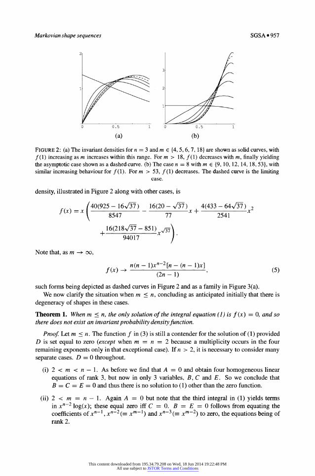
FIGURE 2: (a) The invariant densities for n = 3 and m e {4, 5, 6, 7, 18} are shown as solid curves, with f (1) increasing as m increases within this range. For m > 18, f (1) decreases with m, finally yielding the asymptotic case shown as a dashed curve. (b) The case n = 8 with m e {9, 10, 12, 14, 18, 53}, with similar increasing behaviour for f (1). For m > 53, f (1) decreases. The dashed curve is the limiting

case.

density, illustrated in Figure 2 along with other cases, is

1( 40(925 - 160/7) 16(20 - V/7) 4(433 - 640/7) 2

8547 77 2541

16(218 •/-

- 851)

x4)7 94017

Note that, as m -~ 0o,

n(n - 1)xn-2[n - (n - 1)x] f(x) -•( (5)

(2n - 1)

such forms being depicted as dashed curves in Figure 2 and as a family in Figure 3(a). We now clarify the situation when m < n, concluding as anticipated initially that there is

degeneracy of shapes in these cases.

Theorem 1. When m < n, the only solution of the integral equation (1) is f (x) = 0, and so there does not exist an invariant probability density function.

Proof Let m < n. The function f in (3) is still a contender for the solution of (1) provided D is set equal to zero (except when m = n = 2 because a multiplicity occurs in the four remaining exponents only in that exceptional case). If n > 2, it is necessary to consider many separate cases. D = 0 throughout.

(i) 2 < m < n - 1. As before we find that A = 0 and obtain four homogeneous linear equations of rank 3, but now in only 3 variables, B, C and E. So we conclude that B = C = E = 0 and thus there is no solution to (1) other than the zero function.

(ii) 2 < m = n - 1. Again A = 0 but note that the third integral in (1) yields terms in Xn-2 log(x); these equal zero iff C = 0. B = E = 0 follows from equating the coefficients of xn-1, xn-2 ( xm-1) and xn-3 ( m-2) to zero, the equations being of rank 2.



958 o SGSA R. COWAN AND F K. C. CHEN

6 2

4

2-

0 0.5 1 0 0.5

(a) (b)

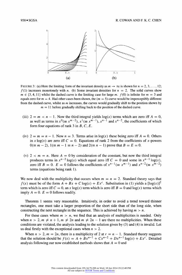
FIGURE 3: (a) Here the limiting form of the invariant density as m -+ oo is shown for n = 2, 3,..., 12; f(1) increases monotonely with n. (b) Some invariant densities for n = 2. The solid curves show m E {3, 4, 11} whilst the dashed curve is the limiting case for large m. f(0) is infinite for m = 3 and equals zero for m = 4. Had other cases been shown, the (m = 5)-curve would be imperceptibly different from the dashed curve, whilst as m increases, the curves would gradually shift to the position shown by

m = 11 before gradually shifting back to the position of the dashed curve.

(iii) 2 = m < n - 1. Now the third integral yields log(x) terms which are zero iff A = 0, as well as terms in xo(= xm-2), X1(( xm-1), xn-1 and Xn-2, the coefficients of which form four equations of rank 3 in B, C, E.

(iv) 2 = m = n - 1. Now n = 3. Terms arise in log(x) these being zero iff A = 0. Others in x log(x) are zero iff C = 0. Equations of rank 2 from the coefficients of x-powers 0(- m - 2), 1(- m - 1 -

n - 2) and 2(- n - 1) prove that B = E = 0.

(v) 2 < m = n. Here A = 0 by consideration of the constant, but now the third integral produces terms in xn-2 log(x) which equal zero iff C = 0 and some in xn-1 log(x), zero iff B = 0. E = 0 follows the coefficients of xn-'1 ( xm-l) and xn-2(= Xm-2) terms (equations being rank 1).

We now deal with the multiplicity that occurs when m = n = 2. Standard theory says that f(x) must be of the form A + Bx + C log(x) + Exc. Substitution in (1) yields a [log(x)]2 term which is zero iff C = 0, an x log(x) term which is zero iff B = 0 and log(x) terms which imply A = 0. E = 0 follows readily.

Theorem 1 seems very reasonable. Intuitively, in order to avoid a trend toward thinner rectangles, one must take a larger proportion of the short side than of the long side, when constructing the next rectangle in the sequence. This is achieved by having m > n.

For these cases where m > n, we find that an analysis of multiplicities is needed. Only when n > 2, m : n + 1, m : 2n and m # 2n - 1 are there no multiplicities. When these conditions are violated, the analysis leading to the solution given by (3) and (4) is invalid. Let us deal firstly with the exceptional cases when n > 2.

When n > 2, m = 2n, there is a multiplicity of 2 at r = n - 1. Standard theory suggests that the solution should be f (x) = A + Bxn-1 + Cxn-2 + Dxn-1 log(x) + Exc. Detailed analysis following our now established methods shows that A = 0 and



Markovian shape sequences SGSA e 959

(1 + c)(c - n)(n - 1)nH B= 4(2n - 1)(1 + c - n)3(c + n)

(1 + c)(n - 1)n4(n + 1) (2n - 1)(2 + c - n)(1 + c - n)(c + n)(6)

(1 + c)(n - 1)2n3(c - n) D=

2(2 + c - n)(1 + c - n)2(c + n)

(1 + c)(1 + c - 2n)(n - 1)n4 E=

(2n - 1)(2 + c - n)(1 + c - n)3(c + n)'

where H := c(n - 1) - 2n[1 - 3n + 2(n + 1)n2]. When n > 2, m = 2n - 1, the multiplicity is now at r = n - 2 so f(x) = A + Bxn-1 +

Cxn-2 + Dxn-2 log(x) + Exc is the candidate. We find that A = 0 and

B= (1 + c)(n - 2)(n - 1)3n (2n - 1)(2 + c - n)(c - 1 + 3n) (1 + c)(3 + c - n)(1 + c - n)nH

C= 4(2n - 1)(2 + c - n)3(c - 1 + 3n) (7) (1 + c)(n - 1)2n2(3 + c - n)

D=- 2(2 + c - n)2(c - 1 + 3n)

(1 + c)(3 + c - 2n)(n - 1)3n E=

(2n - 1)(2 + c - n)3(c - 1 + 3n)'

where now H := nc - 2(2 - 10n + 15n2 - 10n3 + 2n4). When n > 2, m = n + 1, xm-n-l collapses to xo, so the only candidate solution is of the

form f (x) = D + Bxn-1 + Cxn-2 + A log(x) + Exc. The analysis shows that A = 0, and so the log(x) term does not remain in the solution. We also find the other four coefficients and note that they agree with (4), under the substitution m = n + 1 (hence explaining our rather odd juxtaposition of A and D above).

We now deal with the cases when n = 2. When n = 2, m > 5, there is a multiplicity of 2 at r = 0. Standard theory suggests that the solution be f(x) = C + Bx + A log(x) + Dxm-3 + Exc, but it turns out that A = 0 and an (n = 2)-version of (4) gives the other coefficients. Note that, as m -+ oo, f(x) - 2(2 - x)/3, agreeing with (5).

When n = 2, m = 4, the only candidate solution is f(x) = C + Bx + A log(x) + Dx log(x) + Exc where c = 2/3. We find that A = 0 and, for x e (0, 1],

f(x) 2(27- A3) (4663 -464A3) 2(69 - 16A3) 2(131,/ - 149) 2/3 f(x)= - x+ x log(x)+ x

33 3993 363 3993

a result which is consistent with an (n = 2)-version of (6). Finally, when n = 2, m = 3, there is a multiplicity of order 3 at r = 0. Thus we need to

try f(x) = D + Bx + C log(x) + A[log(x)]2 + Exc. The result, which is consistent with (7) when n = 2,isA = B = 0 and,forx e (0,1],

f(x) 605 + 13 111 - og(x)+ 19V- 61 ( V-1)/2 1536 192 1536

Figures 3(b) shows the (n = 2)-cases for a range of m whilst Figure 4 illustrates the invariant densities when m = 2n or 2n - 1 (as does Figure 2(a) in the (n = 3)-case).



960* SGSA R. COWAN AND F. K. C. CHEN

3 3

2 2

1 1

0 0.5 1 0 0.5 1

(a) (b)

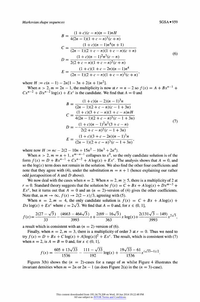
FIGURE 4: The invariant densities for: (a) m = 2n - 1; (b) m = 2n. In both graphs n E {2, 3, 4, 5, 6), with f (1) increasing as n increases.

R QR QR S QR Q

V:

)TT

O P O T P O T P O P

(a) (b) (c) (d)

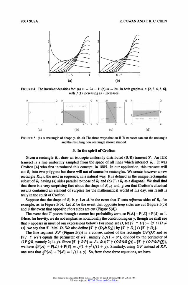
FIGURE 5: (a) A rectangle of shape y. (b-d) The three ways that an IUR transect can cut the rectangle and the resulting new rectangle shown shaded.

3. In the spirit of Crofton

Given a rectangle Rt, draw an isotropic uniformly distributed (IUR) transect T. An IUR transect is a line uniformly sampled from the space of all lines which intersect Rt. It was Crofton [4] who first introduced this concept, in 1885. In our application, this transect will cut Rt into two polygons but these will not of course be rectangles. We create however a new rectangle Rt+l, the next in sequence, in a natural way. It is defined as the unique rectangular subset of Rt having (a) sides parallel to those of Rt and (b) Tn Rt as a diagonal. We shall find that there is a very surprising fact about the shape of Rt+I and, given that Crofton's classical results contained an element of surprise for the mathematical world of his day, our result is truly in the spirit of Crofton.

Suppose that the shape of Rt is y. Let A be the event that T cuts adjacent sides of Rt, for example, as in Figure 5(b). Let X be the event that opposite long sides are cut (Figure 5(c)) and 4 the event that opposite short sides are cut (Figure 5(d)).

The event that T passes through a corner has probability zero, so P{AI} + P{?} + P{-8} = 1. (Here, for brevity, we do not emphasise notationally the conditioning on y, though we shall see that y appears in most of our expressions below.) For some set D, let {T f D} := {T n D # 0}; we say that T 'hits' D. We also define {T f (DI&D2)} by {T f D1} n {T f D2}.

The line-segment RP (Figure 5(a)) is a convex subset of the rectangle OP QR and so

P{T t RP} equals the perimeter of RP, namely 2/(1 + y2), divided by the perimeter of OPQR, namely 2(l+y). Since {T f RP} = U-SUI{T t (OR&RQ)}UIT t (OP&PQ)}, we have 1 PI{A} + PI{X} + P{8} = /(1 + y2)/(1 + y). Similarly, using OP instead of RP, one sees that 1P{BA} + P{Xd} = 1/(1 + y). So, from these three equations, we have




R Q R B Q R Q

X _I.•B

x\ I

Bv V\V

V 1 A

u u ' u

O A P 0 A P 0 P

(a) (b) (c)

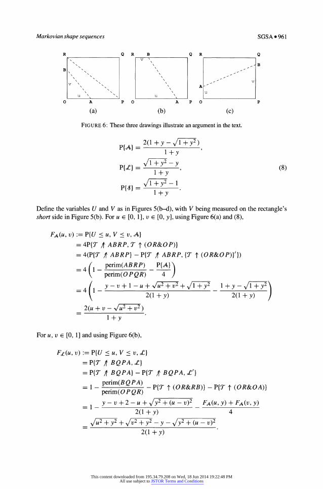
FIGURE 6: These three drawings illustrate an argument in the text.

2(1 + y - 1+y2)

1+y

PI{} I= V/+(8) 1+y

1 + y2 -1

P{8} =

1+y

Define the variables U and V as in Figures 5(b-d), with V being measured on the rectangle's short side in Figure 5(b). For u e [0, 1], v e [0, y], using Figure 6(a) and (8),

FA(u, v) := P{U < u, V < v, A}

= 4P{T /f ABRP, T t (OR&OP)} = 4(P{T j/ ABRP} - P{T /f ABRP, {T f (OR&OP)}'})

=4(1 perim(ABRP) P{A} perim(O P QR) 4

=4 y

- v + 1-u+ N/U2_2+ 11-y2 I+y-V--y 2(1 + y) 2(1 + y)

2(u + v - /u2+v2)

l+y

For u, v e [0, 1] and using Figure 6(b),

Ft.(u, v) := P{U < u, V < v, ?X} = P{T / BQPA, ?} = P{T / BQPA} - P{T / BQPA, q'}

perim(B QPA) = 1 - - P{T t (OR&RB)} - P{T t (OR&OA)} perim(O P QR)

y - v + 2 - u + y2+(u- V)2 FA(u, y) + FA(v, y) 2(1 + y) 4

2 _ + y2 2 _+ - y - y2(u_ - V)2 2(1 + y)



962 e SGSA R. COWAN AND F. K. C. CHEN

Similarly, for u, v e [0, y], using Figure 6(c),

Fs (u, v) := P{U < u, V < v, 4}

2y - u - v + 1 + 1 + (u - v)2 F(1, u) + F(1, v) =1-)2 FA u)FA 2(1 + y) 4

S2+ /1 2- 1 - fl + (u - )2

2(1 + y)

If the shape of Rt+l is X, then P{X > x} = P{X > x, A} + P{X > x, X} + P{X > x, S-}. We now analyse these three terms. For x e [0, 1],

P{X>x,A}=P min -, >x,A

= P{xU < V < U/x, A}

XyU/X Yl UfA (u, v) dvdud+ f Yf(u, v) dv du 0 <x < y (9)

fxy u/x y/x y

=- j fA(u, v)dvdu + j jf A(u, v)dvdu y <x < 1,

where we have introduced one of the improper densities, listed below.

22FA(u, v) 2uv

a2FCe(u, v) y2 ue (U( V2

3/

f2 F ((u, v) 1

aua(u, v) v 2(1 + (u - v)2)3/2(1 + y)

Evaluation of (9) yields

2(1 + y - 1x2 1y2 ) P{X > x, A}l x < y, (10)

(1 + y)N/1-+X2 2y(1 - x) x > y.

(1 + y)1?X2

To evaluate P{X > x, ?}, we define W := IU - VI when ? or - occurs and note that for w E [0, 1],

P{W < w, ?I} = 2 f (u, v)dvdu + ft (u, v)dvdu

w + y2 yw2

(1 + y)/w2?x2




Thus for x e [0, 1],

P{X > X,} = P min W,

>xx

= P{xy < W < y/x, ?}

1?+X2 V/1+y2 - x - y (- x < y (11) (1 + y)_/I+X2

(1 -x)(1 -y) (

+y)lx > y.

(I + y)N1?X2

Similarly, for w E [0, y],

1 + wy- 1?w2 P{W < w, 8}=

(1 + y)•1

+w2

SO,

P{X > x, 8} = P{W > x, 8}

1?+x2 1y2- 1 - xy )= x < y (12)

(1 + y)z/1+ X2 =0 x>y.

Combining (10), (11) and (12), one obtains P{X > x}. Differentiating yields the transition density function

p('ly). Here the dependence on y is emphasised for the first time in our

argument, but there is a surprise! For all y E [0, 1],

l+x p(x I y) = (13)

(1 + x2)3/2 (13)

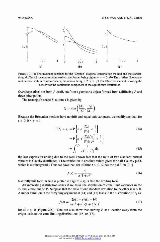
The shape distribution of our new rectangle is actually not dependent on y, the previous shape! This means that, regardless of the shape of Ro, R1 and all subsequent rectangles have shape p.d.f. given by the right-hand side of (13); furthermore all shapes in the sequence are independent. A plot of (13) is shown in Figure 7(a).

Thus the Markov process reaches stationarity after just one step, a phenomenon rarely seen, though a referee has pointed out that this occurs in the Hardy-Weinberg law of mathematical genetics.

4. The link with Brownian motion following Kendall

Consider a point P, initially at the planar origin O. Now let P move as a standardised planar Brownian motion, that is, its cordinates (Xt, Yt) at time t undergo independent standard one-dimensional Brownian motions. At each time t, we form a rectangle with sides parallel to the axes and having OP as a diagonal. How does the shape of this evolving rectangle change? Does it have a limiting distribution?

Our interest in these questions arises from Kendall's work [5] concerning the dynamics of shape for n > 3 randomly-diffusing points in the plane. His notion of shape is inapplicable, however, for n < 3; two points alone do not have a shape and neither does our single point, P.



964 * SGSA R. COWAN AND F. K. C. CHEN

1 1

0.5 1 0.5

0 0.5 1 0 0.5 1 0 0.5 1

(a) (b) (c)

FIGURE 7: (a) The invariant densities for the 'Crofton' diagonal-construction method and the standardised driftless Brownian-motion method, the former being higher at x = 0. (b) The driftless Brownian- motion case with unequal variances, the ratio b being 1, 2 or 3. (c) The Blaschke method, showing the

density for the continuous component of the equilibrium distribution.

Our shape arises not from P itself, but from a geometric object formed from a diffusing P and three other points.

The rectangle's shape St at time t is given by

|% IYtl' lXt "

Because the Brownian motions have no drift and equal unit variances, we readily see that, for t > 0,0 s < 1,

P{St > s}1= Ps < < -1 (14) | Yt I s

=P IXt I / I /I 1I

fl/S 2 = (1 + Z2)

dz, (15)

the last expression arising due to the well-known fact that the ratio of two standard normal variates is Cauchy distributed. (The restriction to absolute values gives the half-Cauchy p.d.f. which is our integrand.) Thus we have that, for all time t > 0, St has the p.d.f. on [0,1]

4 f(s) =

-(1 s2) (16)

Naturally this form, which is plotted in Figure 7(a), is also the limiting form. An interesting distribution arises if we relax the stipulation of equal unit variances in the

x- and y-motions of P. Suppose that the ratio of one standard deviation to the other is b > 0. A minor variation in the foregoing argument at (14) and (15) leads to the distribution of St as

2b(1 + s2)(1 + b2) f(s) = (17) f

(s2 + b2)(1 + b2s2)'

for all t > 0 (Figure 7(b)). One can also show that starting P at a location away from the origin leads to the same limiting distributions (16) or (17).




(a) (b) (c) (a) (b) (c)

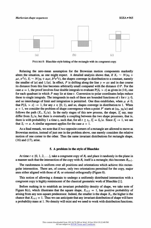
FIGURE 8: Blaschke-style hitting of the rectangle with its congruent copy.

Relaxing the zero-mean assumption for the Brownian motion components markedly alters the situation, as one might expect. A detailed analysis shows that, if Xt -- N(xo + 1t, cr2t), Yt "- N(yo + alt, b2u2t), the shapes converge in distribution to a constant, namely the smaller of lal and 1/Ia I. In effect, P is drifting along the line y = ax and in due course its distance from this line becomes arbitrarily small compared with the distance OP. For the case a = 1, the proof involves four double integrals to evaluate P{St > s} as given in (14), one for each quadrant in which P may lie at time t. Conversion to polar coordinates helps reduce these to single integrals. The integrands in each of these are bounded functions of t for t > 0, and so interchange of limit and integration is permitted. One thus establishes, when

/z # 0, that P{St > s)} 1, for any s E [0, 1), and so, shapes converge in distribution to 1. When a < 1, we consider the problem of shape convergence when a point P' starts at (xo, yo/a) and follows the path (Xt, Yt/a). In the early stages of this new process, the shape, St say, may differ from St/a, but there is eventually a coupling between the two shape processes, that is, there is with probability 1 a time tc such that, for all t > tc, St = St/a. Since St - 1, we see that St - a. A similar argument applies for the case a > 1.

As a final remark, we note that if two opposite corners of a rectangle are allowed to move as Brownian motion, instead of just one in the problem above, one merely considers the relative motion of one corner to the other. Thus the same invariant distributions for rectangle shape, (16) and (17), arise.

5. A problem in the style of Blaschke

At time t E {0, 1, 2, ... }, take a congruent copy of Rt and place it randomly in the plane in a manner such that the intersection of the copy with Rt itself is a rectangle; this becomes Rt+l.

The randomness is uniform over all positions and orientations which achieve this rectangular intersection. There are, of course, only two orientations permitted for the copy, major axes either aligned with those of Rt or oriented orthogonally (Figure 8).

This notion of allowing a domain to undergo a uniformly distributed intersection with a congruent copy is highly reminiscent of the classical geometric work of Blaschke [1].

Before rushing in to establish an invariant probability density of shape, we take note of Figure 8(c), which illustrates that the square shape, Xt+1 = 1, has positive probability of arising from any non-square predecessor. Indeed, the smaller is the shape Xt, the higher is the chance that Xt+l = 1. Thus we can anticipate that any invariant distribution of shape will have a probability mass at 1. No density will exist and we need to work with distribution functions.




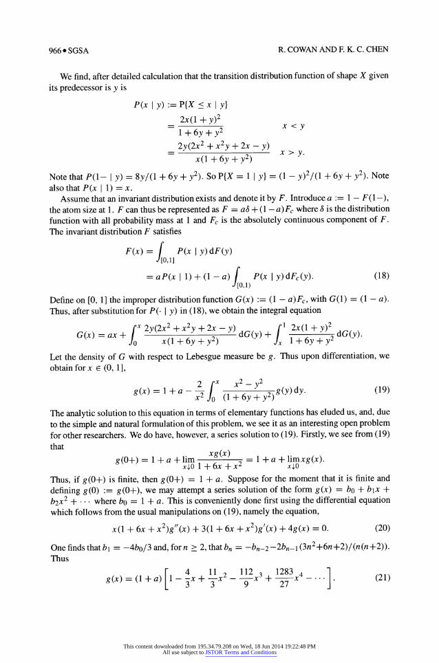
We find, after detailed calculation that the transition distribution function of shape X given its predecessor is y is

P(x I y) := P{X x I y}

2x(1 + y)2 1 + 6y +y2

2y(2x2 + x2y + 2x - y) = x > y. x(1 + 6y + y2)

Note that P(1- I y) = 8y/(l + 6y + y2). So P{X = 1 I y} = (1 - y)2/(1 + 6y + y2). Note also that P(x I 1) = x.

Assume that an invariant distribution exists and denote it by F. Introduce a := 1 - F(1-), the atom size at 1. F can thus be represented as F = aS + (1 - a) Fc where 8 is the distribution function with all probability mass at 1 and Fc is the absolutely continuous component of F. The invariant distribution F satisfies

F(x) = f P(x I y) dF(y) J [0,1]

= aP(x 1) +(1-a)f P(x I y)dFc(y). (18) J [0,1)

Define on [0, 1] the improper distribution function G(x) := (1 - a)Fc, with G(1) = (1 - a). Thus, after substitution for P(- I y) in (18), we obtain the integral equation

Gx 2y(2x2 +x2y + 2x - y) dG(y)+ 1

2x(1 + y)2

S+x(1 + 6y + y2) 1 + 6y +y2

Let the density of G with respect to Lebesgue measure be g. Thus upon differentiation, we obtain for x e (0, 1],

2 fx x2 _ 2

g(x) = +a -

2,

x2 6y2) g(y)dy. (19)

x2 (1 + 6y + y2)

The analytic solution to this equation in terms of elementary functions has eluded us, and, due to the simple and natural formulation of this problem, we see it as an interesting open problem for other researchers. We do have, however, a series solution to (19). Firstly, we see from (19) that

xg(x) g(O+) = 1 + a + lim = 1 + a + limxg(x).

x0O 1 + 6x + x2 x0

Thus, if g(0+) is finite, then g(0+) = 1 + a. Suppose for the moment that it is finite and

defining g(O) := g(0+), we may attempt a series solution of the form g(x) = bo + blx + b2x2 + -

-... where bo = 1 + a. This is conveniently done first using the differential equation which follows from the usual manipulations on (19), namely the equation,

x(1 + 6x + x2)gN(x) + 3(1 + 6x + x2)g'(x) + 4g(x) = 0. (20)

One finds that bl = -4bo/3 and, for n > 2, that bn = -bn-2-2bn-1 (3n2+6n+2)/(n(n+2)).

Thus

[ 4 211 112 1283x g(x)

= (l + a) 1 - 1-x + -x

2 - 3 - . (21) 3

3x9 ?2 ..7(1




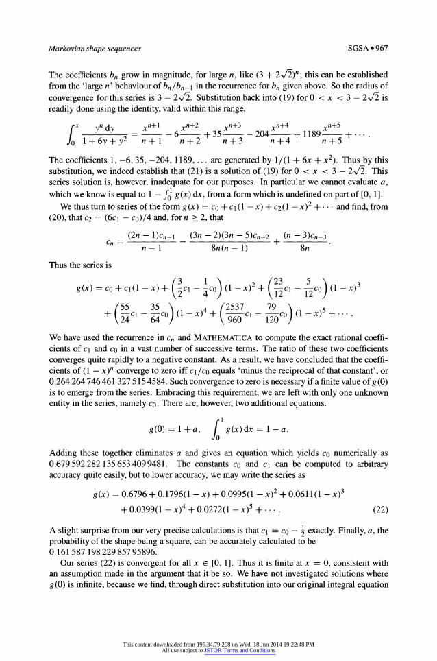
The coefficients bn grow in magnitude, for large n, like (3 + 2V/2)n; this can be established from the 'large n' behaviour of bn/bn-1 in the recurrence for bn given above. So the radius of

convergence for this series is 3 - 2A/2. Substitution back into (19) for 0 < x < 3 - 2A/2 is readily done using the identity, valid within this range,

fx yn dy xn+1 xn+2 xn+3 xn+4 n+5

= - - 6- + 35 - 204 + 1189- + o1 + 6y + y2 n + 1 n+2 n+3 n+4 n+5

The coefficients 1, -6, 35, -204, 1189, ... are generated by 1/(1 + 6x + x2). Thus by this substitution, we indeed establish that (21) is a solution of (19) for 0 < x < 3 - 2V/2. This series solution is, however, inadequate for our purposes. In particular we cannot evaluate a, which we know is equal to 1 - fo g(x) dx, from a form which is undefined on part of [0, 1].

We thus turn to series of the form g(x) = co + Ci(1 - x) + c2(1 - x)2 + .. and find, from (20), that c2 = (6cl - co)/4 and, for n > 2, that

(2n - 1)cn-1 (3n - 2)(3n - 5)Cn-2 (n - 3)Cn-3 Cn = +-

n- 1 8n(n - 1) 8n

Thus the series is

g(x) = co + ci(1 - x) + C- co (1 - x)2

• C -

c•

(1 - x)3 2 4 12 12

(55 35 (2537 79 l- 5CO (1 -x)4?+ 0Cl- CO (1-x)5+.. 24 64960 120

We have used the recurrence in cn and MATHEMATICA to compute the exact rational coefficients of cl and co in a vast number of successive terms. The ratio of these two coefficients converges quite rapidly to a negative constant. As a result, we have concluded that the coefficients of (1 - x)n converge to zero iff cl/co equals 'minus the reciprocal of that constant', or 0.264 264 746 461 327 515 4584. Such convergence to zero is necessary if a finite value of g (0) is to emerge from the series. Embracing this requirement, we are left with only one unknown entity in the series, namely co. There are, however, two additional equations.

g(0)= 1 +a, g (x)dx= 1- a.

Adding these together eliminates a and gives an equation which yields co numerically as 0.679 592 282 135 653 409 9481. The constants co and Cl can be computed to arbitrary accuracy quite easily, but to lower accuracy, we may write the series as

g(x) = 0.6796 + 0.1796(1 - x) + 0.0995(1 - x)2 + 0.0611(1 - x)3

+ 0.0399(1 - x)4 + 0.0272(1 - x)5 + . .. . (22)

A slight surprise from our very precise calculations is that Cl = co - ? exactly. Finally, a, the probability of the shape being a square, can be accurately calculated to be 0.161 587 198 229 857 95896.

Our series (22) is convergent for all x e [0, 1]. Thus it is finite at x = 0, consistent with an assumption made in the argument that it be so. We have not investigated solutions where g (0) is infinite, because we find, through direct substitution into our original integral equation




(19), that (22) is a solution. From the obvious qb-recurrence of the Markov process, it is the unique invariant solution to our problem and we need look no further. Figure 7(c) plots the solution g.

Whilst our series is a worthwhile solution to our problem, the failure to solve this problem analytically has frustrated us. We have, however, solved a related problem with a different hitting measure. If the congruent shape is rotated with probability p > 0, fixed for all iterations, with position being uniformly distributed over all possible rotated positions, or is not rotated with probability q := 1 - p, again with uniform distribution over these possible positions, we can establish that

p - 4p3/21 a=

1 + p - 4p3/21'

where

fo

y, fdy

I (1 + y)2'

whilst g(x) = (1 - a)4'1-ix-P-1. When p = 1, the probability mass a at x = 1 is (3 - 4 log 2)/(4 - 4 log 2) and, given that the rectangle is not a square, its shape is uniformly distributed on [0, 1]. When p = 0, shapes degenerate to 0.

References

[1] BLASCHKE, W. (1936). Vorlesungen iiber Integralgeometrie. Deutsch Verlag Wissenschaft, Berlin. [2] CHEN, F. K. C. AND COWAN, R. (1999). Invariant distributions for shapes in sequences of randomly-divided

rectangles. Adv. Appl. Prob. 30, 1-14. [3] COWAN, R. (1997). Shapes of rectangular prisms after repeated random division. Adv. Appl. Prob. 29, 26-37. [4] CROFTON, M. W. (1885). Probability. Encyclopaedia Britannica, 9th edn., 19, 768-788, London. [5] KENDALL, D. G. (1977). The diffusion of shape. Adv. Appl. Prob. 9, 428-430. [6] MANNION, D. (1988). A Markov chain of triangle shapes. Adv. Appl. Prob. 20, 348-370. [7] MANNION, D. (1990). Convergence to collinearity of a sequence of random triangle shapes. Adv. Appl. Prob.

22, 831-844. [8] REINYI, A. AND SULANKE, R. (1963). Uber die konvexe Hiill von n zufaillig gewdihlten Punkten. Z. Wahr-

scheinlichkeitsth. 2, 75-84.



four interesting problems concerning markovian shape sequences

Documents