fog computing for heterogeneous multi-robot … · fog computing for heterogeneous multi-robot...
TRANSCRIPT
FOG COMPUTING FOR HETEROGENEOUS MULTI-ROBOT
SYSTEMS WITH ADAPTIVE TASK ALLOCATION
Siddharth Bhal
Thesis submitted to the Faculty of the
Virginia Polytechnic Institute and State University
in partial fulfillment of the requirements for the degree of
Master of Science
in
Computer Engineering
Ryan K. Williams, Chair
Pratap Tokekar
Michael S. Hsiao
June 22, 2017
Blacksburg, Virginia
Keywords: Task Allocation, Cloud Robotics, Fog Computing, Multi-Robot Systems,
Internet of Things
Copyright 2017, Siddharth Bhal
FOG COMPUTING FOR HETEROGENEOUS MULTI-ROBOT
SYSTEMS WITH ADAPTIVE TASK ALLOCATION
Siddharth Bhal
(ABSTRACT)
The evolution of cloud computing has finally started to affect robotics. Indeed, there have
been several real-time cloud applications making their way into robotics as of late. Inher-
ent benefits of cloud robotics include providing virtually infinite computational power and
enabling collaboration of a multitude of connected devices. However, its drawbacks include
higher latency and overall higher energy consumption.
Moreover, local devices in proximity incur higher latency when communicating among them-
selves via the cloud. At the same time, the cloud is a single point of failure in the network.
Fog Computing is an extension of the cloud computing paradigm providing data, com-
pute, storage and application services to end-users on a so-called edge layer. Distinguishing
characteristics are its support for mobility and dense geographical distribution. We pro-
pose to study the implications of applying fog computing concepts in robotics by developing
a middle-ware solution for Robotic Fog Computing Cluster solution for enabling adaptive
distributed computation in heterogeneous multi-robot systems interacting with the Internet
of Things (IoT). The developed middle-ware has a modular plug-in architecture based on
micro-services and facilitates communication of IOT devices with the multi-robot systems.
In addition, the developed middle-ware solutions support different load balancing or task
allocation algorithms. In particular, we establish that we can enhance the performance of
distributed system by decreasing overall system latency by using already established multi-
criteria decision-making algorithms like TOPSIS & TODIM with naive Q-learning and with
Neural Network based Q-learning.
FOG COMPUTING FOR HETEROGENEOUS MULTI-ROBOT
SYSTEMS WITH ADAPTIVE TASK ALLOCATION
Siddharth Bhal
(GENERAL AUDIENCE ABSTRACT)
Technologies like robotics are advancing at a rapid pace and have started affecting various
aspects of human lives. A lot more focus is now on collaborative robotics which focuses on
robots designed to work with each other. A swarm/fleet of robots has unique use cases like
disaster rescue missions.
In this thesis, we explore various ways to enable efficient and effective communication be-
tween robots in a multi-robot environment. We also compare different methods a robot
can communicate and share its workload with other robots in a collaborative environment.
Finally, we propose a new approach to reducing robots communication cost and optimizing
process through which it shares its workload with other robots in real time using machine
learning techniques.
Acknowledgement
First, I feel proud being the first graduate student of my committee chair and research
advisor, Dr. Ryan K Williams. I want to give him my deepest gratitude for his continuous
guidance, encouragement, and patience throughout my graduate education. I am grateful
to him for showing trust in my capabilities and funding me. His extensive knowledge and
scientific thinking enlighten me to this day and ever after.
I want to thank Dr. Pratap Tokekar and Dr. Michael S. Hsiao for being in my advising
committee and providing assistance and feedback on my research. I also grateful to Dr.
Chao Wang for being my interim research advisor when I started my graduate life.
I am also grateful to Mr. Srdjan Miocinovic and Mr. Arthur James for being outstanding
mentors during my summer internship at Qualcomm and illustrating the application of my
research in consumer industry.
I want to thank my fellow lab mates - Pratik, Jun, Remy, Larkin, and Anand for providing
constant help in my work. I appreciated and enjoyed the working experience. will cherish
my spent in lab as it was always enriching experience.
I also want to thank my fellow mates - Tapas, Sarthak, Abhilash, and Nahush. It would have
been a difficult stay in Blacksburg away from my homeland (India) without their company.
Finally, I want to thank my parents - DP Singh and Sunita Singh for providing a constant
source of motivation throughout my life and encouraging me to lead my life on principles.
vi
Contents
1 Introduction and Background 1
1.1 Cloud Computing . . . . . . . . . . . . . . . . . . . . . . . . . . . . . . . . . 2
1.2 Fog Computing . . . . . . . . . . . . . . . . . . . . . . . . . . . . . . . . . . 3
1.3 Cloud Robotics . . . . . . . . . . . . . . . . . . . . . . . . . . . . . . . . . . 5
1.3.1 History . . . . . . . . . . . . . . . . . . . . . . . . . . . . . . . . . . . 6
1.3.2 Big Data . . . . . . . . . . . . . . . . . . . . . . . . . . . . . . . . . . 8
1.4 Load balancing . . . . . . . . . . . . . . . . . . . . . . . . . . . . . . . . . . 10
1.4.1 Static load balancing . . . . . . . . . . . . . . . . . . . . . . . . . . . 12
1.4.2 Dynamic Load Balancing . . . . . . . . . . . . . . . . . . . . . . . . . 14
1.5 Motivation . . . . . . . . . . . . . . . . . . . . . . . . . . . . . . . . . . . . . 24
1.6 Thesis Outline and Contributions . . . . . . . . . . . . . . . . . . . . . . . . 27
vii
2 System Architecture 29
2.1 Requirements . . . . . . . . . . . . . . . . . . . . . . . . . . . . . . . . . . . 29
2.2 Architecture Primer . . . . . . . . . . . . . . . . . . . . . . . . . . . . . . . . 31
2.2.1 Layered pattern . . . . . . . . . . . . . . . . . . . . . . . . . . . . . . 31
2.2.2 Client Server Architecture . . . . . . . . . . . . . . . . . . . . . . . . 33
2.2.3 REST Architecture . . . . . . . . . . . . . . . . . . . . . . . . . . . . 34
2.2.4 Master Slave Architecture . . . . . . . . . . . . . . . . . . . . . . . . 34
2.2.5 Pipes and Filters Architecture . . . . . . . . . . . . . . . . . . . . . . 35
2.2.6 Broker Pattern . . . . . . . . . . . . . . . . . . . . . . . . . . . . . . 35
2.2.7 Peer to Peer Pattern (p2p) . . . . . . . . . . . . . . . . . . . . . . . . 36
2.2.8 Event Bus Pattern . . . . . . . . . . . . . . . . . . . . . . . . . . . . 36
2.2.9 Micro-services Architecture . . . . . . . . . . . . . . . . . . . . . . . 37
2.2.10 Criteria for Choosing Architecture . . . . . . . . . . . . . . . . . . . . 38
2.3 Architecture . . . . . . . . . . . . . . . . . . . . . . . . . . . . . . . . . . . . 38
2.3.1 Cloud Layer . . . . . . . . . . . . . . . . . . . . . . . . . . . . . . . . 40
2.3.2 Edge Layer . . . . . . . . . . . . . . . . . . . . . . . . . . . . . . . . 41
2.3.3 Device Layer . . . . . . . . . . . . . . . . . . . . . . . . . . . . . . . 43
viii
3 Implementation 44
3.1 Cloud layer . . . . . . . . . . . . . . . . . . . . . . . . . . . . . . . . . . . . 44
3.2 Edge layer . . . . . . . . . . . . . . . . . . . . . . . . . . . . . . . . . . . . . 48
3.3 Device Layer . . . . . . . . . . . . . . . . . . . . . . . . . . . . . . . . . . . 57
4 Task Allocation 62
4.1 MCDM . . . . . . . . . . . . . . . . . . . . . . . . . . . . . . . . . . . . . . 62
4.2 TOPSIS . . . . . . . . . . . . . . . . . . . . . . . . . . . . . . . . . . . . . . 63
4.3 TODIM . . . . . . . . . . . . . . . . . . . . . . . . . . . . . . . . . . . . . . 65
4.4 Naive Q-learning . . . . . . . . . . . . . . . . . . . . . . . . . . . . . . . . . 68
4.4.1 Q learning with TOPSIS . . . . . . . . . . . . . . . . . . . . . . . . . 71
4.4.2 Q learning with TODIM . . . . . . . . . . . . . . . . . . . . . . . . . 72
4.5 Q-learning using Neural Network . . . . . . . . . . . . . . . . . . . . . . . . 73
4.5.1 Q learning with TOPSIS using Neural Network . . . . . . . . . . . . 74
4.5.2 Q learning with TODIM using Neural Network . . . . . . . . . . . . 75
5 Results 76
5.1 Experimentation Setup . . . . . . . . . . . . . . . . . . . . . . . . . . . . . . 76
ix
5.2 Fixed Parameters . . . . . . . . . . . . . . . . . . . . . . . . . . . . . . . . . 81
5.3 Results Analysis . . . . . . . . . . . . . . . . . . . . . . . . . . . . . . . . . . 83
6 Conclusion 97
Bibliography 101
Appendices 112
x
List of Figures
1.1 Fog Computing . . . . . . . . . . . . . . . . . . . . . . . . . . . . . . . . . . 5
1.2 RoboEarth Architecture design 2013 [57] . . . . . . . . . . . . . . . . . . . . 8
2.1 Network OSI Model . . . . . . . . . . . . . . . . . . . . . . . . . . . . . . . . 32
2.2 Fog Computing Middleware Layers . . . . . . . . . . . . . . . . . . . . . . . 39
3.1 Cloud Node Modules . . . . . . . . . . . . . . . . . . . . . . . . . . . . . . . 45
3.2 Cloud Broker Sequence Diagram . . . . . . . . . . . . . . . . . . . . . . . . . 47
3.3 Edge Node Modules . . . . . . . . . . . . . . . . . . . . . . . . . . . . . . . . 48
3.4 Edge Cloud Sequence Diagram . . . . . . . . . . . . . . . . . . . . . . . . . . 49
3.5 Edge Node Module Dependency . . . . . . . . . . . . . . . . . . . . . . . . . 52
3.6 Edge Node Cloud Ready Sequence . . . . . . . . . . . . . . . . . . . . . . . 53
3.7 Edge Node Neighbor Ready Sequence . . . . . . . . . . . . . . . . . . . . . . 54
xi
3.8 Edge Node Charting Ready . . . . . . . . . . . . . . . . . . . . . . . . . . . 55
3.9 Edge Node Neighbor Msg Broker Sequence . . . . . . . . . . . . . . . . . . . 55
3.10 DJI Matrice 100 Overview . . . . . . . . . . . . . . . . . . . . . . . . . . . . 58
3.11 NVIDIA TX2 Development Board . . . . . . . . . . . . . . . . . . . . . . . . 58
3.12 Orbitty Carrier Board for NVIDIA TX2 . . . . . . . . . . . . . . . . . . . . 59
3.13 IoT Device: Artik Board . . . . . . . . . . . . . . . . . . . . . . . . . . . . . 59
3.14 IoT Device: Libelium Node . . . . . . . . . . . . . . . . . . . . . . . . . . . 60
3.15 DJI Matrice 100 with Orbitty Carrier for Nvidia TX2 . . . . . . . . . . . . . 60
3.16 Edge Device Sequence Diagram . . . . . . . . . . . . . . . . . . . . . . . . . 61
4.1 Prospect Theory [37] . . . . . . . . . . . . . . . . . . . . . . . . . . . . . . . 66
4.2 Q-learning State Transition Diagram . . . . . . . . . . . . . . . . . . . . . . 68
4.3 Q-table for a system with m states and n actions . . . . . . . . . . . . . . . 70
4.4 Single Layer Perceptron . . . . . . . . . . . . . . . . . . . . . . . . . . . . . 73
5.1 Nodes in Experimentation Setup . . . . . . . . . . . . . . . . . . . . . . . . . 77
5.2 Components used in Experimentation . . . . . . . . . . . . . . . . . . . . . . 77
5.3 Device Node . . . . . . . . . . . . . . . . . . . . . . . . . . . . . . . . . . . . 78
5.4 CPU Utilization of Edge Node during Stress Task . . . . . . . . . . . . . . . 84
xii
5.5 Free Memory on Edge node during Stress Task . . . . . . . . . . . . . . . . . 85
5.6 Number of Active Contexts on Edge during Stress Task . . . . . . . . . . . . 86
5.7 Number of Active Contexts on Cloud during Stress Task . . . . . . . . . . . 87
5.8 Cloud to Local offloading Ratio during Stress Task . . . . . . . . . . . . . . 88
5.9 Neighbor to Local offloading Ratio during Stress Task . . . . . . . . . . . . . 89
5.10 Cloud Latency during Stress Task . . . . . . . . . . . . . . . . . . . . . . . . 90
5.11 First Neighbor Latency during Stress Task . . . . . . . . . . . . . . . . . . . 91
5.12 Second Neighbor Latency during Stress Task . . . . . . . . . . . . . . . . . . 92
5.13 Jobs Ingress rate from device node during Stress Task . . . . . . . . . . . . . 93
5.14 Moving Avg of System Latency for Jobs during Stress Task . . . . . . . . . . 94
5.15 Overall System Latency for Jobs during Stress Task . . . . . . . . . . . . . . 95
xiii
List of Tables
1.1 Fog Computing vs Cloud Computing . . . . . . . . . . . . . . . . . . . . . . 4
5.1 Fixed Parameters for algorithms . . . . . . . . . . . . . . . . . . . . . . . . . 82
5.2 Short Notation for Algorithms . . . . . . . . . . . . . . . . . . . . . . . . . . 83
xiv
Chapter 1
Introduction and Background
Cloud computing has revolutionized software engineering in the last decade. Cloud com-
puting is an umbrella term for cloud applications and cloud platforms. A cloud application
is a software application with two components. One component runs locally on the client
whereas the other component runs on cloud infrastructure. Cloud applications run on cloud
platforms which consist of multiple remote servers running in data centers. In this chapter
we will introduce cloud computing and fog computing. We will list the benefits of architec-
tures based on fog computing over cloud computing. Finally, we will discuss the importance
of load balancing and discuss how fog computing and load balancing algorithms helped us
in designing a Fog computing based computing cluster for multi-robot systems interacting
with IoT devices.
1
Siddharth Bhal Introduction and Background 2
1.1 Cloud Computing
As per NIST (National Institute of Standards and Technology) [48], Cloud computing is
defined as: “Cloud computing is a model for enabling ubiquitous, convenient, on-demand
network access to a shared pool of configurable computing resources (e.g., networks, servers,
storage, applications, and services) that can be rapidly provisioned and released with minimal
management effort or service provider interaction. This cloud model is composed of five
essential characteristics, three service models, and four deployment models.”
Essential characteristics of cloud computing are on-demand self-service, broad network ac-
cess, resource pooling, rapid elasticity and measured service. Various software deployment
models are used such as Software as a Service, Infrastructure as a service and Platform as a
service.
• Software as a Service (SaaS): It is a software delivery model where clients access appli-
cations running on cloud infrastructure. The consumers usually accesses applications
through a thin client like a web browser. Most SaaS solutions are based on multi-tenant
architectures whereas other solutions use technologies like virtualization. The client
isn’t allowed to modify any resources running on cloud infrastructure like operating
system, network, storage or running instances of an application.
• Platform as a Service(PaaS): Clients are provided with a platform where they can
deploy their application utilizing libraries provided by the platform. Customers can
thus avoid developing their own infrastructure for development and testing of their
Siddharth Bhal Introduction and Background 3
application. Clients control minimal configuration of application hosting environment
and deployed application.
• Infrastructure as a Service(IaaS): The consumer is only provided with computing infras-
tructure, and they can develop and deploy an arbitrary application with the freedom
to choose their choice of operating system. Generally limited access to the network is
provided to consumer.
Cloud computing is considered as the 4th industrial revolution following the first revolution
of mechanization of the industry using steam, the second with mass production of electricity
and third was industry automation using electronics.
1.2 Fog Computing
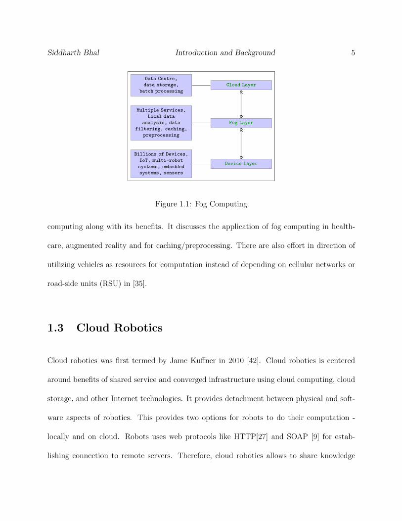
Fog computing (also known as Edge computing) is an extension of the cloud computing
paradigm. It provides compute, storage and networking resources on the edge (or fog)
layer of a network which sits between end users/devices (service subscriber layer) and cloud
computing data centers (cloud layer) as shown in Figure 1.1.
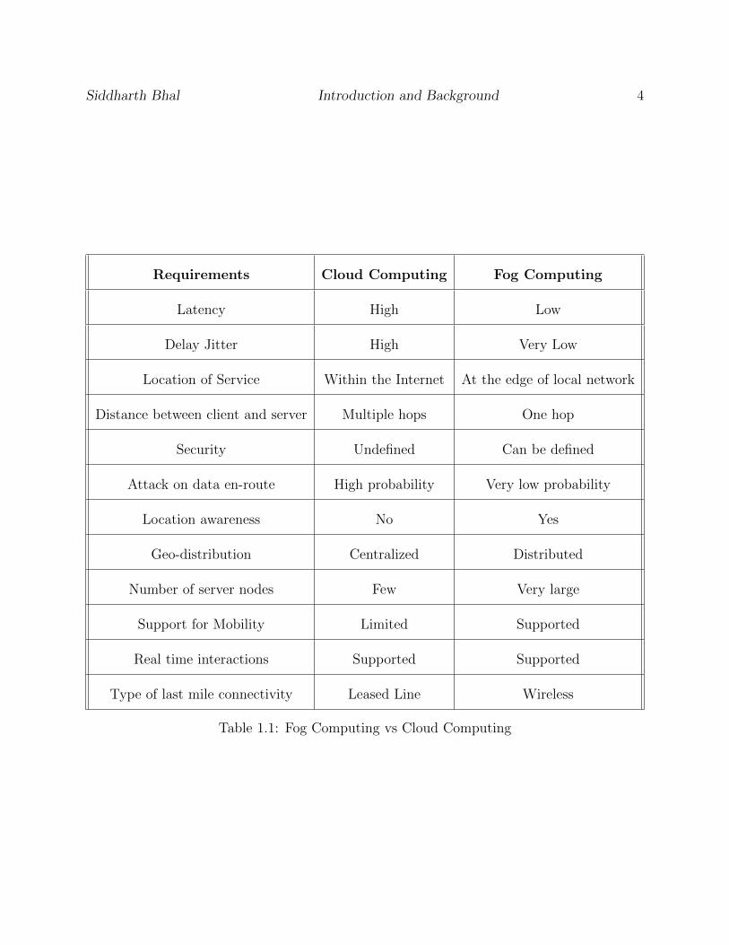
Some of the differences between Fog computing and Cloud computing as per [3] are shown
in Table 1.1.
[21] shows the implementation of Robotic SLAM using fog computing. [18] discusses on fog
computing principles, architecture and applications. It provides a reference model for fog
Siddharth Bhal Introduction and Background 4
Requirements Cloud Computing Fog Computing
Latency High Low
Delay Jitter High Very Low
Location of Service Within the Internet At the edge of local network
Distance between client and server Multiple hops One hop
Security Undefined Can be defined
Attack on data en-route High probability Very low probability
Location awareness No Yes
Geo-distribution Centralized Distributed
Number of server nodes Few Very large
Support for Mobility Limited Supported
Real time interactions Supported Supported
Type of last mile connectivity Leased Line Wireless
Table 1.1: Fog Computing vs Cloud Computing
Siddharth Bhal Introduction and Background 5
Data Centre,
data storage,
batch processing
Cloud Layer
Multiple Services,
Local data
analysis, data
filtering, caching,
preprocessing
Fog Layer
Billions of Devices,
IoT, multi-robot
systems, embedded
systems, sensors
Device Layer
Figure 1.1: Fog Computing
computing along with its benefits. It discusses the application of fog computing in health-
care, augmented reality and for caching/preprocessing. There are also effort in direction of
utilizing vehicles as resources for computation instead of depending on cellular networks or
road-side units (RSU) in [35].
1.3 Cloud Robotics
Cloud robotics was first termed by Jame Kuffner in 2010 [42]. Cloud robotics is centered
around benefits of shared service and converged infrastructure using cloud computing, cloud
storage, and other Internet technologies. It provides detachment between physical and soft-
ware aspects of robotics. This provides two options for robots to do their computation -
locally and on cloud. Robots uses web protocols like HTTP[27] and SOAP [9] for estab-
lishing connection to remote servers. Therefore, cloud robotics allows to share knowledge
Siddharth Bhal Introduction and Background 6
among robots and offload compute-intensive tasks like image processing, voice recognition,
etc. It also enables robots to utilize new capabilities added by cloud services.
Cloud robotics is a unified standalone system relying on the network to support powerful
computation, storage and memory requirements in its operation. Many different systems
falls under cloud computing like teleoperation of a group of mobile robots like UAVs [43],
[49] or warehouse robots [17], [4] and home automation systems. Cloud robotic systems are
quite similar to automation systems which have limited local processing power useful in cases
of network failure and unreliable network. One of the recent examples of cloud robotics is
Google’s self-driving car [33]. The self-driving car has sensors and software created to detect
vehicles, cyclists, pedestrians and road work from distance. The car makes a decision based
on different models created from local 3D view superimposed with high resolution updated
maps fetched from the cloud.
1.3.1 History
The first manufacturing automation system was developed in the 1980s by General Mo-
tors implementing the Manufacturing Automation Protocol (MAP) [36]. There were many
proprietary protocols developed until the World wide web became widely adopted which
uses HTTP[s] over IP protocol for networking purposes [52]. The first time an industrial
robot was teleoperated by users using an Internet browser was in 1994 [29]. This led to the
beginning of the field of networked robotics. [40], [47]. Due to the wide variety of bene-
Siddharth Bhal Introduction and Background 7
fits, IEEE Robotics and Automation Society instituted a committee on Networked Robots.
The main focus of Springer handbook on robotics [44] was on networked telerobots and
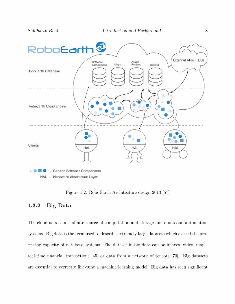
networked robots respectively. A recent project RoboEarth [69] started in 2009 is a cloud
robotic infrastructure which allows robots to collaborate, offload computation and store and
share information. RoboEarth cloud engine is used to provide powerful computation to the
robots in system.. Datastores are used to store knowledge generated by human and machine
in machine readable format. Datastores can consist of software components, maps, action
recipes, objects, etc. RoboEarth also supports Robot Operating System (ROS) compatible
components for high-level control of the robot.
Cloud platforms such as RoboEarth provides the following advantages:
• Facilitate Cooperation: cloud helps to facilitate cooperation among device nodes.
• Offload computation: Computationally intensive tasks like planning, probabilistic in-
ference, and mapping can be offloaded to cloud.
• Provides global datastore: Scalable storage provided by cloud layer database can be
used to store and share information.
• Multiple robots can learn about the environment using other’s experience. This is a
method of learning by sharing experiences.
• Instead of individually programming robot, a developer can create robot task instruc-
tion.
Siddharth Bhal Introduction and Background 8
Figure 1.2: RoboEarth Architecture design 2013 [57]
1.3.2 Big Data
The cloud acts as an infinite source of computation and storage for robots and automation
systems. Big data is the term used to describe extremely large datasets which exceed the pro-
cessing capacity of database systems. The dataset in big data can be images, video, maps,
real-time financial transactions [45] or data from a network of sensors [70]. Big datasets
are essential to correctly fine-tune a machine learning model. Big data has seen significant
Siddharth Bhal Introduction and Background 9
interest in the field of computer vision as processing images/videos is computationally in-
tensive and require substantial resources. Image datasets like ImageNet [20] and PASCAL
object classes dataset [26] have been used for object’s surrounding recognition. An aug-
mented reality application using photo collection is created with processing in the Cloud
[28]. Blending Internet images with human feedback provided a robust object learning tech-
nique shown in [34]. Deep learning is a subfield of machine learning concerned with artificial
neural networks. Deep learning has shown great results in supervised learning with improved
performance with respect to to the amount of trained data. Thus deep learning can take
advantage of big data [19] and is majorly used in computer vision [41], [58] and grasping [46].
Grasping is a novel challenge and cloud computing can help in learning grasping strategies
[15], [51]. Defining the standard for representing data like trajectories and maps has been
an active research field [55], [67] and [68].
DAvinCi [5] is a computing cluster software framework based on cloud architecture providing
scalability and massive advantages of Map-Reduce Hadoop framework. Map-Reduce makes a
system more scalable and available with advantages of parallel processing and simple model of
programming. DAvinCi has been successfully used for doing FastSLAM using Map-Reduce.
[39] also shows RSi Research Cloud using Robot Service Network Protocol (RSNP) for re-
ceiving information via network. RSNP is a standardized protocol for providing services to
robots. Benefits of using standardized protocol is increased compatibility with various ven-
dors. Examples of services supported by RSNP are Disaster Information Service, Monitoring
service, Robot map etc.
Siddharth Bhal Introduction and Background 10
1.4 Load balancing
Load balancing is a process of even distribution of computing workload among computing
entities in a distributed network. It helps in reducing the possibility of tasks remaining in
waiting queue of scheduler when there are existing idle servers in the distribution system.
Load balancing plays a vital role in parallel cloud computing and distributed systems. One
of the key characteristics attributed to it is an increase in scalability. An increase in traffic
can hamper the performance of the system, and load balancing avoids it with system scal-
ability. Moreover, it can help in making a system more redundant. Categorization of load
balancing algorithms can be found in [30], [71] and [11].
Some of the advantages of load balancing as mentioned in [30] are:
• Scalability is the ability of computing system to handle growing amount of work. With
the virtualization of services, scalability has become a fundamental aspect of large scale
system. Optimal scalability is not possible without effective load balancing technique.
• It helps to handle a sudden surge in traffic. A sudden increase in traffic can potentially
bog down some nodes in a distributed network and thereby make them unusable.
Indirectly it affects the performance of the overall system.
• Load balancing can improve a system’s redundancy. System redundancy helps to
increase system up time. Ignoring this key criterion can result in suboptimal per-
Siddharth Bhal Introduction and Background 11
formance. It can help to restrict the impact of hardware failures on system uptime
significantly. The load balancing algorithm can schedule the same task on multiple
servers making the system more robust and thus it can respond in case of single node
failure as well.
• It helps to make the system highly available. Redundancy helps to achieve reduced
downtime making the system more highly available.
• Systems without support for load balancing have limited ways to recover from a failure
of nodes. Load balancers allow multiple ways to recover from system failure. It can
divert traffic to other nodes. Meanwhile, the failed node itself tries to recover its failed
part. Thus it allows the system to be more resilient to failures with minimal effect on
client/users.
• It can decrease response latency. By scheduling the same task on multiple servers, it
can improve response time.
• It helps in making systems more flexible. By allowing system nodes to join and leave
the network at runtime.
• It allows a server to perform bookkeeping and maintenance tasks, thereby reducing
system’s downtime.
• By distributing load uniformly among nodes, it helps in optimal system resource uti-
lization.
Siddharth Bhal Introduction and Background 12
• It helps in superior resource utilization and also helps in energy conservation.
• It helps to enhanced Quality of Service (QoS) and maintaining Service Level Agree-
ments (SLA).
• It improves response time for request while keeping acceptable delays.
• It can facilitate to reduce communication overhead in system.
• It helps to improve job throughput.
• It improves ability to adapt to runtime changes in task inflow rate.
• It helps to maintain system stability by accounting for time spent in passing up jobs
among nodes instead of processing them in the case of high inflow of jobs.
Above mentioned advantages of load balancing algorithms can help to improve reliability,
performance and maintenance of heterogeneous autonomous networks. It also helps in im-
proving the scalability of a heterogeneous system with robots, IOT and cloud agents. There-
fore it is essential to come up with an optimal load balancing strategy for our fog computing
cluster. We will discuss in detail about our load balancing and task allocation strategies in
Chapter Task Allocation.
1.4.1 Static load balancing
Static load balancing is the distribution of computing workload among computing entities
in a distributed network. It’s a non preemptive scheme utilizing a priori information about
Siddharth Bhal Introduction and Background 13
the system, resource requirements per job and communication overhead to make offloading
decision. Nodes distribute their work without considering the current state of the system
when making assignment decisions. In other words, it makes an assumption on the state of
the system when making scheduling decisions. When there are minor changes in the system
with respect to time, static load balancing can produce excellent results. This category of
algorithms have less computation overload and do not need to gather environmental data
through agents due to the assumption of a fixed state of the environment. Static load
balancing algorithms perform better than their counterparts when the system is static in
nature. Static load balancing algorithms [65], [53], [63], [66] and [8] can be either stateless
or stateful. Stateless algorithms make their decisions without considering the state of the
system.
Examples of stateless algorithms are:
• Round Robin Algorithm: It is one of simplest load balancing algorithms where a
node allots its workload evenly among distributed nodes in turn. The node keeps
on circularly distributing its workload endlessly without priority. It’s not the most
efficient algorithm since it assumes the same capabilities for each node and performs
inadequately when jobs take unequal processing time.
• Weighted Round Robin: Weights define the capacity of nodes to handle tasks. Each
neighboring node is assigned weights representing the relative capability of a node com-
pared to other nodes. Nodes with higher weight receive more workload for processing.
Siddharth Bhal Introduction and Background 14
Stateful algorithms consider state of the system while making their decisions.
Examples of stateful algorithms are:
• Central Manager Algorithm: The load balancing node acts as a master in the master
slave configuration. The master node keeps track of a load index of slave nodes which
are responsible for updating the master periodically. This algorithm outperforms others
when multiple nodes in a distributed network act as load balancing nodes. Central
design creates one of the biggest limitations as it restricts scalability of the system.
• Threshold Algorithm: Nodes in a distributed system are divided into three separate
categories namely under-load, medium or overloaded. A node is only required to update
its private copy of load indexes of neighbors when its load class changes. This limits
the number of messages exchanged as compared to periodically updating the central
node with load state. A key benefit of this approach is less inter-node communication
compared to the Central Manager Algorithm.
• Dynamic Round Robin: Nodes are assigned weights based on real time data like CPU
utilization and utilized memory.
1.4.2 Dynamic Load Balancing
Unlike static load balancing, dynamic load balancing involves uniformly distributing loads,
thus moving tasks from busy servers to underloaded servers [30] and [23] . Dynamic schemes
[10], [23], [38], [62], [61], [6], [7], [22] and [32] spend more time in migration of jobs than
Siddharth Bhal Introduction and Background 15
static load balancing schemes. It can make better job offloading decisions than static schemes
but can suffer from excessive interprocess communication by continuously monitoring load
index of other nodes. Dynamic load balancing algorithms makes use of three strategies:
information strategy, transfer strategy and location strategy to make an offloading decision.
Information strategy
Information strategy is responsible for collecting information about nodes in a system [23]
and [71]. It acts as an information provider for the transfer strategy and location strategy.
An information strategy providing information of all other nodes in the system will yield
extra communication overhead in our system. Therefore it is recommended to come up
with a strategy for collecting information of nodes in the system which is limited and can
provide useful parameters for making load allocation decisions. In [23] it was concluded
that comprehensive information strategies may not provide a significant advantage over
other approaches(semi-detailed one). A fully distributed load balancing strategy will be
more likely to have a comprehensive or detailed information strategy. The amount of extra
information needed for load balancing algorithms is an overhead. Thus, there is a trade-off
between the number of messages exchanged between nodes and the frequency of messages
exchanges.

Siddharth Bhal Introduction and Background 16
Transfer strategy
Transfer strategy decides which particular jobs can be offloaded to other nodes. There are
various factors which need to be considered while making the transfer strategy decision.
These include
• Job queue length,
• CPU utilization,
• Job resource requirement,
• Job execution time, and
• % of CPU idle time
A naive approach is to schedule jobs without considering the specific nature of the scheduled
job. In this approach nodes only need to look for queue length of neighboring nodes to
make their decision. One of the advantages of this approach is ubiquity, in other words,
this method can be applied to any system regardless of its specific characteristics. One of
the disadvantages of treating all jobs similarly is that it leaves a lot of space for improving
the performance of the system. Dynamic Load Balancing Algorithms using this approach
are [23], [14] and [24]. Other approaches [73], [31] and [64] make use of jobs information
collected in real time execution when making scheduling decisions. [64] shows an approach
to utilize history of execution of the job to make future decisions. We will observe that in
Siddharth Bhal Introduction and Background 17
this study after optimization, smaller job are mostly executed locally. [14] used an approach
based on future computation requirement based on statistics.
Location strategy
Location strategy decides the target node to which a task can be offloaded. It helps in
selecting the destination node. It is one the most important parts of a load balancing
algorithm. Location strategies will try to balance the overloaded nodes and underloaded
nodes in the system. The criteria used in selecting destination nodes can be current job
queue length, CPU utilization, % of CPU idle time at remote nodes, etc. CPU ready job
queue length is one of the simplest ways to gauge the future load on remote nodes. Location
strategy also makes use of other information collected by information strategy to make its
decision of which destination node to offload the current task. Some of the examples of
location strategies used to select destination node are:
Random
A destination node is randomly selected, and the task is offloaded for execution. The selected
remote node only executes the job if its resource availability is above a predefined threshold.
Otherwise remote node offloads tasks to a new destination node. This algorithm may result
in continuous offloading of the task without executing it. To avoid this situation, we can
make use of TTL (time to live). Each hop the job encounters reduces the TTL value by
1. After multiple offloading decisions on the same job the TTL value will reduce to zero,
Siddharth Bhal Introduction and Background 18
during which the last node has to forcefully execute the job and reply with results. Here
the assumption is that the job is only offloaded to nodes which are able to execute the job.
In other words nodes have the required capabilities to execute the job. Random Transfer
strategy performs much better than the system with no load balancing strategy. We will
be using this strategy as a baseline to compare our strategy and other global information
strategy algorithms.
Probing
In Probing, a node is continuously probing a set of neighboring node to find a suitable des-
tination node. Destination nodes often provides better execution time than local execution
time. Three different types of probing location strategies are threshold, greedy and shortest.
Threshold location probing strategy is very similar to random location strategy. The only
difference is that in threshold location probing strategy, a random node is selected from
a subset of all nodes that the local nodes is aware of. They are called neighbors of local
nodes. Thus a random node for task offloading is selected from the neighborhood and it is
verified whether the task can be offloaded. If the selected destination node’s load is above
a predefined threshold, a new node is selected. We only continue selecting new nodes a
preset number of times. After that job is executed locally. This is very similar to the TTL
notion used in the random load balancing strategy. Threshold strategy has shown to be a
substantial improvement over random strategy.
Siddharth Bhal Introduction and Background 19
Greedy strategy is similar to threshold strategy. In greedy strategy, remote nodes are con-
sidered as destination nodes in cyclic fashion instead of random order. For the next task,
the cycle continues where it was stopped earlier. It’s shown that greedy strategy performs
better than threshold strategy [14].
Shortest strategy is a variant of threshold strategy where a random subset of neighbors are
chosen and each node is probed for its load vector. The nodes which have smallest load are
considered for offloading the task. The task is offloaded if the selected node with least load
has load below a threshold, otherwise the task is executed locally. Shortest strategy being a
wiser variant of threshold strategy, it does not perform much better than threshold strategy.
Negotiation
This transfer strategy is mainly used in dynamically distributed algorithms. In this strategy,
nodes negotiate the tasks among themselves.
There are two ways of conducting negotiations:
• Bidding
In bidding, overloaded nodes start the bidding process to offload some tasks in its
queue to other nodes. Other nodes bid according to their available resources. This
strategy is also called sender-initiated since negotiation starts only when a sender sends
Siddharth Bhal Introduction and Background 20
a new task and any node in the system moves to overloaded state. When any node in
the system moves to overloaded state, it broadcasts a bid request MSG to all nodes in
the system. This MSG contains the current load of overloaded nodes and information
about the jobs this node is willing to offload to others nodes. Receiving nodes only
respond if their load level is less than originator node’s load level. In case the load of
the receiving node is higher than originator node, it simply ignores the MSG and does
not respond. Receiving nodes in return respond with bid messages which include their
load vector and information about jobs which they are interested in. The overloaded
node then chooses the remote node with best bid (in our case its the one with the least
load) and offloads jobs to it. One potential problem with this strategy is if under-load
nodes win lots of bids simultaneously and is unable to execute them in a timely fashion.
The solution to this problem would be to place a restriction on the number of bidding
process a node can participate in at a time. [13] shows a consensus based auction for
robust task allocation with decentralized focus with the assumption of predetermined
hierarchical levels of nodes in partitions/clusters.
• Drafting
Drafting strategy also contains a negotiation phase which is receiver initiated. Nodes
are classified according to the volume of loads they carry. They could be overloaded,
underloaded or neutral loaded. A node can classify themselves in the category accord-
ing to predefined thresholds. In drafting strategy, a node is responsible for updating
its status to all remote nodes in the system. Whenever a node moves from a neutral
Siddharth Bhal Introduction and Background 21
loaded category to underloaded category, it finds all overloaded nodes in its private
copy of systems resources and broadcasts a draft request MSG to all overloaded nodes.
The draft request message represents the willingness of the under-load node to han-
dle more jobs processing. Overloaded nodes that receive draft request messages will
reply with a response containing information about nodes which can be offloaded to.
The original underloaded nodes receive all responses and choose remote node on some
criteria and unicast draft select MSG. If receiving node is still overloaded, it transfers
some of its jobs with original node. Drafting strategies are shown to perform better
than bidding strategy according to [54].
Category of Dynamic load balancing algorithms based on system topology are:
• Distributed - All nodes execute load balancing algorithm. Generate more messages.[10],
[62] and [6], [25], [50], [60] and [32]. Distributed load balancing algorithms are more
chatty due to more inter-process communication required as each node need to be aware
of other nodes statuses compared to non-distributed algorithms. One of the advantages
being it’s more fault tolerant since one node fault will not affect the working of other
nodes.
• Non-Distributed - Only some nodes in distributed system runs Load Balancing algo-
rithms.
Types of Dynamic load balancing algorithms based on how nodes coordinates with each
Siddharth Bhal Introduction and Background 22
other:
• Coordinated - Nodes work together to achieve a global objective. For example nodes
will coordinate to reduce overall system latency.
• Non Cooperative - Each node works together independently toward local goal. For
example to improve local response latency.
We have discussed some of the common issues which deal with all the dynamic load balancing
algorithms. Dynamic algorithms need to be stable for system stability. An efficient algorithm
wont be useful in many scenarios if it is not stable. Therefore stability is one the important
characteristic of a dynamic load balancing algorithm.
System stability
System stability is one of the most import characteristics, and dynamic load balancing
algorithm needs to be stable in a distributed system. Three criteria used to define the
stability of system are:
1. Processor thrashing: A system should not enter into the state of processor thrashing
where nodes in the system are simply exchanging messages between them without
doing any actual job execution.
2. Load difference: The difference between the load of two nodes in a subset of nodes in
Siddharth Bhal Introduction and Background 23
the system should always lie within a threshold limits.
3. Response time during burst arrival: During any burst arrival of jobs to a specific
node should not make it unusable and nodes should be able to response within some
threshold response time.
Load measurements
Many dynamic algorithm’s transfer strategy makes use of load information of other nodes
when making a decision. What exactly does an algorithm utilize to make the offloading
decision? The answer to this question is algorithm dependent, but in general, some of the
quality load descriptors are:
• Job queue length,
• CPU utilization,
• CPU idle time,
• Amount of unfinished work at a node,
• Available resources like free memory, and
• Job resource requirements
Job queue length is one of the most common load descriptors used in several dynamic load
balancing algorithms. It is mainly considered as the base to benchmark other load descriptors
Siddharth Bhal Introduction and Background 24
for a dynamic algorithm. When a system only uses Job queue length as a load descriptor,
it involves less computation and is simple to fetch its value. Despite the simplicity, it is
showed job resource requirement as better load descriptor than job queue length especially
when we can categorize jobs according to their requirements and jobs are simply served in
round robin fashion.
Performance measurements
Different load balancing algorithms utilize different performance indexes to measure their
performance. Ultimately load balancing algorithms affects system performance, and there-
fore performance index provides a significant way to gauge the utility of load balancing
algorithm. There are both system oriented and user-oriented performance indexes available.
Some of the system oriented performance indexes are system throughput and resource utiliza-
tion. Examples of user-oriented performance indexes are mean response time of distributed
systems and mean job execution time. One of the commonly used performance index by
many load balancing algorithms is system mean response time.
1.5 Motivation
Although cloud computing provides capability to offload tasks and enable robots to share
information, it suffers from higher latency issues. Another disadvantage is the higher cost
of cloud bandwidth which can limit the bandwidth usage by system units. One can always
Siddharth Bhal Introduction and Background 25
lose connection to cloud which can deprive robot of basic functionality. Moreover, robots are
often tasked in environments that do not support always-on cloud connection (e.g. search
and rescue in remote environments).
Data and applications are processed in a cloud, which is a time consuming task for large
data. To overcome the disadvantage of cloud computing for robotic systems, we propose
a new architecture for computing cluster middle-ware to support multi-robot systems with
IOT (Internet Of Things).
We decided to base our design on Fog Computing architecture. Fog computing architecture is
an extension of cloud architecture with an extra edge layer near end users. This layer helps
Fog computing provide the benefits of location awareness and lower latency with respect
to cloud. Fog computing also overcomes the problem of limited bandwidth which cloud
is suffering from and is expected to grow worse in future especially with the exponential
growth of IOT devices. Other drawback of cloud is that cloud bandwidth can be costly. For
these reasons we feel Fog computing architecture to be more suitable for real-time robotic
application services.
Cloud robotics has been on rise recently. It provides high scalability for system and ability
for system nodes to learn and share their data. Cloud also serve as database which can
store information about the environment, routes, object maps, learned models etc. Cloud
facilitates nodes in a multi-robot system to collaborate with each other. This enables a
robotic unit to share its learning with other units in system. For example, a robot fleet doing
SLAM (Simultaneous localization and mapping) of environment can share their progress with
Siddharth Bhal Introduction and Background 26
each other to save time as well as computation. For example, an exploratory robot doing
SLAM can fetch the information available for current location and can start building on
available information about environment rather than building from scratch.
Many robots including mobile robots and UAV (unmanned aerial vehicle) have limited com-
putation power with limited battery life. This make it essential to find a way to do remote
computation. Cloud computing is a potential solution for this scenario. There are already
commercial cloud solutions available like Google Cloud, Amazon Web Services and Microsoft
Azure. A cloud solution provides robot system a remote brain for computation as well as
enable nodes to share data with peer nodes in system.
Cloud is assumed to have infinite computation power which make it always good choice for
heavy computation task due to its support for parallelized processing capability as well.
Limitations
Although Cloud and Fog computing provides lots of benefits to multi-robot systems. Still
real time communication for mobile robots can be challenging. Also cloud computing cannot
be used for all basic functionality especially for non-intensive tasks due to higher latency.
Siddharth Bhal Introduction and Background 27
1.6 Thesis Outline and Contributions
In this thesis we contribute to cloud robotics literature by designing & developing a robotic
computing cluster based on Fog computing for heterogeneous multi-robot systems. We also
develop a task allocation algorithm which can be used with computing cluster with goal of
reducing overall system latency.
In Chapter System Architecture we discuss the design of our middle-ware based on Fog
computing architecture which acts as remote brain by providing capabilities and compute
services for remote execution. Middle-ware has the capability to offload tasks to other nodes
running on edge layer as well as can offload them to cloud. Multiple alternatives for task
offload rises the need for efficient task allocation algorithm.
In Chapter Implementation we discuss implementation of edge layer nodes, device nodes
and cloud nodes. We talk about the classification of different services at each node and
multiple communication interfaces supported.
In Chapter Task Allocation we discuss about task allocation algorithms based on Multi
Criteria Decision Making (MCDM), which can be used with our Fog Computing Cluster
middle-ware. We introduce two MCDM algorithms, TOPSIS and TODIM. We compare
the performance of random algorithm with TOPSIS and TODIM. We found both TOPSIS
and TODIM outperformed random algorithms. We further investigate the use of model free
reinforcement learning technique called Q-learning. We found Q-learning further enhanced
the performance for both TOPSIS and TODIM algorithms for our system.
Siddharth Bhal Introduction and Background 28
In Chapter Results, we talk about our experimental setup and discuss obtained results
and compare performance of TOPSIS and TODIM algorithm along with Q-learning based
TOPSIS and TODIM algorithm. We also look into performance of naive Q-learning model
with respect to Neural Network based Q-learning model algorithms.
Finally we conclude in Chapter Conclusion about the experiment and discuss takeaways
and future prospects of the project.
Chapter 2
System Architecture
In this chapter, we will go over the requirements for the design of Fog computing cluster for
heterogeneous multi-robot systems. We will discuss different types of software architecture
and their characteristics. Thereafter, we choose an architecture suitable for our requirements.
Finally, we will discuss components of chosen software architecture.
2.1 Requirements
Our requirement was to design a multi-robot computing cluster providing inherent benefits
of fog computing listed in section 1.2. Section 1.5 outlines the advantages of Fog computing
over currently popular Cloud computing paradigm. We needed a platform solution which
can support heterogeneous devices from multiple vendors including IOT devices and robots.
IOT market has already shown enormous growth, and it is expected to continue in future.
29
Siddharth Bhal System Architecture 30
IOT sector has attracted multiple vendors due to widespread application in various systems.
This move has encouraged developers and researchers to develop system solutions supporting
multiple vendors.
The framework also needs to be extensible with support for actuators as well as sensor
devices. Sensors are the passive device in the system which is continuously publishing their
data to the network. On the other hand, actuators have the capability of taking action.
There are particular data flow optimizations which can be used in sensor only architecture
but may not be optimal for the requirement of a multi-robot cluster with IOT devices (sensors
and actuators). In our case, robots (like quad-copters) aren’t stationary but are continuously
moving. Continuous movement can sometimes result in unstable connection and can have
frequent disconnections with adjacent connecting layer. In a case of frequent disconnections,
the framework should have the capability to handle disconnection and support reconnection
of the device on another system node. The framework is also required to support multiple
tasks, and therefore particular consideration has to be given to designing one with different
task contexts support at each system component.
Based on our requirements, we had to choose suitable software architecture. Our chosen
design should help us provide desired Quality of Service (QoS) and Service Level Agreements
(SLA).
Siddharth Bhal System Architecture 31
2.2 Architecture Primer
Architectural decisions define the high-level design of a system. Minute system implemen-
tation details do not account for greater issues across the entire system. After finalizing
an architecture design, one can use design patterns to implement their chosen architecture
design.
Architecture pattern defines the organization schema for software systems. One can start
with dividing their system into subsystem and assigning responsibilities for each one of them.
Design patterns help us to design system fulfilling the requirements for a software architec-
ture. There could be many design pattern for implementing same software architecture.
Design patterns help us to reuse the solution someone else came up with to a particular
problem. It is an excellent way to utilize the expertise of experienced developers. A de-
sign pattern is building around some core fundamental guidelines and many times address
nonfunctional requirements. Some of the available software architectural patterns are sum-
marized in the following sections.
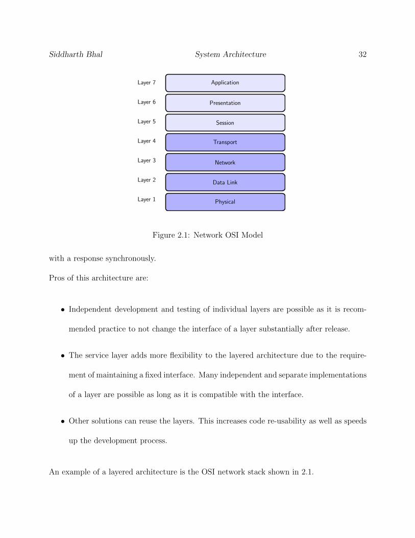
2.2.1 Layered pattern
A layered architecture has the complete solution divided into layers. Each layer has an
interface which the upper layer utilizes. A layer can only access the interface of its next
lower layer, and most of the calls are made synchronously. Most of the time a request
generated by an upper layer travels all the way down to the lowest layer and travels back
Siddharth Bhal System Architecture 32
Layer 7
Layer 6
Layer 5
Layer 4
Layer 3
Layer 2
Layer 1
Application
Presentation
Session
Transport
Network
Data Link
Physical
Figure 2.1: Network OSI Model
with a response synchronously.
Pros of this architecture are:
• Independent development and testing of individual layers are possible as it is recom-
mended practice to not change the interface of a layer substantially after release.
• The service layer adds more flexibility to the layered architecture due to the require-
ment of maintaining a fixed interface. Many independent and separate implementations
of a layer are possible as long as it is compatible with the interface.
• Other solutions can reuse the layers. This increases code re-usability as well as speeds
up the development process.
An example of a layered architecture is the OSI network stack shown in 2.1.
Siddharth Bhal System Architecture 33
In the OSI Model, the application layer can support HTTP, FTP or SMTP protocol. Sim-
ilarly, the transport layer can be an implementation of TCP, UDP or SPX protocol. The
network layer can provide support for IP or ICMP protocol.
One of the biggest disadvantages of this architecture is maintainability of layers and defining
abstraction beforehand.
2.2.2 Client Server Architecture
In the client-server architecture, a client always invokes a request which is served by a
server. Servers could reside in a different process/machine, and therefore inter-process com-
munication is used to facilitate communication between client and server. Servers are always
running, and a client interactively interacts with servers.
The client-server architecture is similar to the layered architecture with the server being a
lower layer than the client. A server can serve multiple clients. Either server or client should
maintain session information.
When server keeps state information of the client, it’s called a stateful server. When a client
is responsible for storing and maintaining session information, the server is referred to as a
stateless server.
Siddharth Bhal System Architecture 34
Disadvantages of the client-server architecture includes an overhead of inter-process commu-
nication. It can add extra complexity when many clients want to access the same function
on the server. Like accessing a URL for a website.
2.2.3 REST Architecture
A REST (REpresentational State Transfer) architecture is similar to client-server architec-
ture with the difference that communication is stateless. It allows a client to repeat multiple
same queries without any side effects. The client can access resources from a server by
accessing a URL. Many web applications make use of REST architecture.
2.2.4 Master Slave Architecture
In this architecture, multiple slave nodes are connected to a single master node. The master
node is responsible for distributing tasks among slaves.
This architecture is mostly suitable for parallel computation or batch processing. This
architecture can be used to make a system more fault tolerant. Although, it is still very
susceptible to master failure. If the master starts scheduling tasks on more than one node,
it makes the system more fault tolerant. This architecture can only be applied to a problem
that can be subdivided.
Siddharth Bhal System Architecture 35
2.2.5 Pipes and Filters Architecture
This architecture is mainly used to process streams of data. Filters are modules of the
system which do uniform processing on input data and outputs it. With the advent of
machine learning and big data, this architecture has seen wide usage lately. Especially in
IOT, data needs to be transformed, and Filters help in doing it. This architecture is mainly
data driven with data transformation functions used.
A compiler is an example of pipe and filter pattern along with Lexical analyzers as well. This
architecture supports processing data in real-time as filters can process data in real-time,
i.e. it doesn’t wait to consume all data and then process it afterward.
Some of the benefits of this pattern are easy maintainability of filters. Filters can be reused
in other pipelines development. Development of filters is also comparatively easier due
to having a defined interface. But, maintenance of the interface and data transformation
between filters can create overhead. Also, an optimal way needs to be found out to store
intermediate results from filters.
2.2.6 Broker Pattern
A broker is responsible for communication between different services. Services register them-
selves with the broker and when a client requests a service, the broker redirects the client to
their desired destination. The broker architecture is more prevalent in distributed architec-
tures. A broker also provides the interface which a client can access to utilize services and
Siddharth Bhal System Architecture 36
the broker takes care of distributing tasks among running servers.
2.2.7 Peer to Peer Pattern (p2p)
It is a symmetric architecture where a node can behave as a client or a server. The role
of a node is dynamic and can change from server to client during runtime. Like the broker
pattern, work is divided among peers but unlike the broker pattern, peers are not equally
privileged. An example of a p2p system is Bittorrent. This pattern is mainly used in dis-
tributed applications. A peer to peer architecture is scalable since there are no master/server
nodes and provides more fault tolerance than other architectures. One of the biggest disad-
vantages of this architecture is there is no guarantee of Quality of Service (QoS) and Service
Level Agreements (SLA).
2.2.8 Event Bus Pattern
In this pattern, an event bus acts as a message broker. Listeners subscribe to topics, and
whenever an event is published to a Topic, all its listeners are notified. Both publishing and
listening of events happen asynchronously. Event driven systems are mainly used in cloud
applications and financial applications. One of the problems with event distribution system
is scalability. Since all other processes are dependent on event bus to receive notification, it
can bog down the system once software goes on a large scale. Also, ordering and storage of
messages have to be considered when using this architecture design pattern.
Siddharth Bhal System Architecture 37
[59] discusses steps to choose an architectural style to fit a given problem. One should
consider sequential/pipelined architecture if the problem can be divided into subtasks. One
should go for closed loop control architecture if we require continuous controlling action.
2.2.9 Micro-services Architecture
The micro-service architecture is a software architecture where the system is divided into
software components called services. The services communicate with each other using APIs.
It allows each service implementation to be language independent. Each service has a distinct
purpose and concentrates on a single task.
Main features of Micro-service architecture are:
• Componentization allows for each micro-service to be upgraded and replaced.
• It allows the system to be more resilient since one micro-service failure doesn’t affect
the working of other software components
• It follows single responsibility principle.
• It is easier to make changes to the system as it is easily understandable
• Each micro-service is language and technology independent which allows choosing the
best technology for each service.
• It also allows ease of service deployment and enables services to be deployed in different
ratio.
Siddharth Bhal System Architecture 38
2.2.10 Criteria for Choosing Architecture
One should also consider following factors when choosing an architecture:
• Maintainability - An architecture should be easily maintainable after the initial devel-
opment of a system is complete.
• Re-usability - Re-usability avoids duplication of code and thus helps in fewer bugs in
the system.
• Performance - Performance is key criteria especially for real-time systems.
• Fault tolerance - Due to dynamic nature of system and movement of device nodes,
fault tolerance is required characteristics for a heterogeneous multi-robot system.
2.3 Architecture
We found no single architecture pattern was able to satisfy all our requirements. Therefore,
we made use of multiple architectural patterns in designing our system. Due to benefits of
fog computing, we decided to base our design on fog computing architecture and break our
system into three components as shown in 2.2:
1. Cloud node component: We decided to use Event Bus pattern to facilitate communica-
tion with different micro-services running on the cloud. Event Bus pattern also helps
edge nodes to listen for events from the cloud.

Siddharth Bhal System Architecture 39
Edge Layer
Edge Node Edge Node Edge Node Edge Node
Cloud Layer
Cloud Node
Device Layer
Device NodeDevice Node Device Node
Legend
Node Cluster
Figure 2.2: Fog Computing Middleware Layers
2. Edge node component: Due to the requirement of communication with similar neigh-
boring nodes, we used peer to peer pattern for communication with neighboring nodes.
The client-server architecture is used for establishing communication with cloud node
where edge nodes act as a client for a server running on cloud node. Event Bus pattern
is used to publish topics for other neighboring nodes.
3. Device node component: This component makes use of REST APIs and Web-Socket
(WS) to access edge node services.
Siddharth Bhal System Architecture 40
2.3.1 Cloud Layer
On cloud layer, the centralized cloud infrastructure provides a pool of shared computation
and storage resources for real-time tasks. Therefore networked robots can use virtually infi-
nite computing power provided by cloud and can take benefits of a large volume of provided
storage. Ample storage enables to store a significant amount of information regarding the
environment and can provide behaviors learned from the history of cloud-enabled robots.
Salient features of cloud component are:
• The cloud uses a micro-service architecture which improves fault tolerance as well as
helps in reduced development time. With this approach, it also takes less amount of
time for a new developer to understand a complex system.
• The server-client architecture is the basis of framework design where cloud nodes act
as a server and edge nodes act as the client for cloud-edge communication.
• The cloud works as the central entity in the complete solution providing services to
both edge and device nodes.
• It provides virtually unlimited computing resources as well as storage resources for
device layer nodes
• Heartbeats are used to keep track of operating units connected to the system.
• Device registry is maintained on cloud and continuously updated when nodes join or
leave the system.
Siddharth Bhal System Architecture 41
• Cloud maintains a list of all devices connected to the system.
• Authentication can be either done on edge layer or cloud layer. For edge layer authen-
tication, each edge device needs to store authentication information. Instead, we chose
authentication on cloud layer as it acts as a common link for communication within
different subsystem networks.
• Device management is a feature of this layer which is responsible for authenticating
and onboarding devices.
• It records the status of all current edge devices.
2.3.2 Edge Layer
The Edge layer is responsible for data collection, aggregation, and acts as a control point for
devices in the device layer.
Salient features of the edge component are:
• Edge nodes supports offloading tasks within the edge layer and to the cloud.
• A plugin architecture provides ad hoc solution supporting different communication
protocols and task plugins. Capability to add support for the new task using plugins
is especially useful.
• The micro-service architecture provides more scalability and performance as one can
Siddharth Bhal System Architecture 42
assess factors such as utilization, speed and response time across the platform and fine
tune performance.
• It also assists in providing authentication and device management with the help of
cloud.
• It is responsible for the orchestration of device nodes in the Device layer.
• Each edge node maintains computation power and storage states of peer nodes.
• Supports service discovery of other nodes present in the local network using multi-cast
DNS.
• It also contributes to making the system more fault tolerant. In the case of loss of
connectivity between edge layer and cloud layer, devices will remain connected with
edge layer.
• It can behave as a local cache storage and can be useful in the distribution of high
bandwidth content.
• It helps to make cloud layer application agnostic to device layers’ implementation.
• It contributes to achieving lower latency for devices as opposed to directly communi-
cating to faraway cloud/data center.
• It also helps to reduce network traffic as less data is transmitted to cloud from local
devices.
• It facilitates to achieve near real-time data analysis of the system.
Siddharth Bhal System Architecture 43
2.3.3 Device Layer
The device layer is the lowest layer in network hierarchy and consists of autonomous units
like quad-copters, ground robots, mobile robots, UAV, sensors, and actuator units.
Salient features of the device component are:
• Devices can be organized in the group thus making it possible to do group activities
including broadcasting and offloading tasks within groups.
• Mesh networking protocols like Zigbee and Bluetooth Mesh can be used for Tasks’
offloading among device nodes part of the same group.
• In case direct interaction between devices is not possible, the same behavior is achieved
with the help of edge layer acting as an intermediary in communication. Edge layer
application can be easily extended using plugins.
• Communication medium can be bidirectional or unidirectional
• Device nodes can use services of edge node using different communication protocols
like web-socket or REST APIs.
Chapter 3
Implementation
In this chapter we will go through actual implementation details of system architecture design
we came up in Chapter System Architecture. We will talk about the platform and software
dependencies for middle-ware. As shown in Figure 5.1 we will discuss implementation details
about components running in each layer.
3.1 Cloud layer
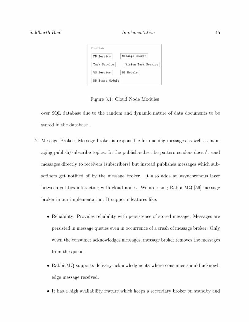
Each node of the cloud consists of the following modules as shown in Figure 3.1
1. DB Service: Db service provides database service to cloud nodes. It is responsible
for storing and handling persistent system information. We are using the No-SQL
database, MongoDB [12] in our implementation. We preferred a No-SQL database
44
Siddharth Bhal Implementation 45
Cloud Node
DB Service Message Broker
Task Service Vision Task Service
WS Service OS Module
MB Stats Module
Figure 3.1: Cloud Node Modules
over SQL database due to the random and dynamic nature of data documents to be
stored in the database.
2. Message Broker: Message broker is responsible for queuing messages as well as man-
aging publish/subscribe topics. In the publish-subscribe pattern senders doesn’t send
messages directly to receivers (subscribers) but instead publishes messages which sub-
scribers get notified of by the message broker. It also adds an asynchronous layer
between entities interacting with cloud nodes. We are using RabbitMQ [56] message
broker in our implementation. It supports features like:
• Reliability: Provides reliability with persistence of stored message. Messages are
persisted in message queues even in occurrence of a crash of message broker. Only
when the consumer acknowledges messages, message broker removes the messages
from the queue.
• RabbitMQ supports delivery acknowledgments where consumer should acknowl-
edge message received.
• It has a high availability feature which keeps a secondary broker on standby and
Siddharth Bhal Implementation 46
switches in case the primary broker fails.
• Supports multiple messaging protocols like AMQP, STOMP and MQTT. In our
implementation, we are using AMQP 0.9.1 protocol for exchanging messages to
message broker.
3. Task Service: It is responsible for handling multiple different tasks supported by the
platform. It is a wrapper service over other individual task services. Individual task
service provides benefits of handling all task queries in separate module following sep-
aration of concerns principle.
4. OS Modules: This module is responsible for getting OS environment parameters like
current CPU usage, CPU idle time, free memory usage etc. It also exports Application
Programming Interfaces (APIs) which other modules can utilize for their functionality.
5. MB Stats Module: This module is used to monitor statistics of queues in running
message broker instance. Stats are published on Edge Node Topics. Decision-making
algorithms like task offloading make use of statistics like pending message in queues to
make their offloading decision.
6. WS Service: This module is responsible for accepting all web-socket communication
from other nodes of the system. It also facilitates all control services. Control ser-
vices include initialization, nodes registration, nodes on-boarding and node’s services
registration.
Siddharth Bhal Implementation 47
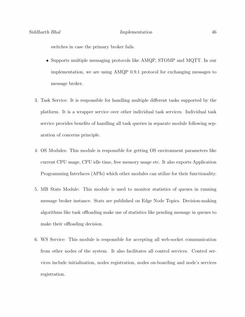
:Cloud Node :Cloud Message Broker
publish Topics osenv
return valuesstart consuming Req Messages
Figure 3.2: Cloud Broker Sequence Diagram
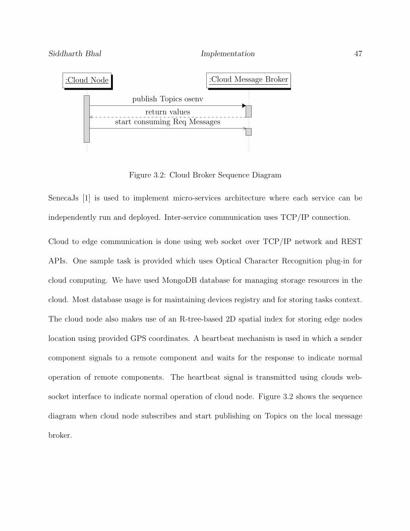
SenecaJs [1] is used to implement micro-services architecture where each service can be
independently run and deployed. Inter-service communication uses TCP/IP connection.
Cloud to edge communication is done using web socket over TCP/IP network and REST
APIs. One sample task is provided which uses Optical Character Recognition plug-in for
cloud computing. We have used MongoDB database for managing storage resources in the
cloud. Most database usage is for maintaining devices registry and for storing tasks context.
The cloud node also makes use of an R-tree-based 2D spatial index for storing edge nodes
location using provided GPS coordinates. A heartbeat mechanism is used in which a sender
component signals to a remote component and waits for the response to indicate normal
operation of remote components. The heartbeat signal is transmitted using clouds web-
socket interface to indicate normal operation of cloud node. Figure 3.2 shows the sequence
diagram when cloud node subscribes and start publishing on Topics on the local message
broker.
Siddharth Bhal Implementation 48
Edge Node
DB Service Message Broker
Task Service Neighbor Service
OS Module REST Service
Core Service Offload Service
Edge WS Server Vision Task Service
Cloud Client MB Stats Module
Figure 3.3: Edge Node Modules
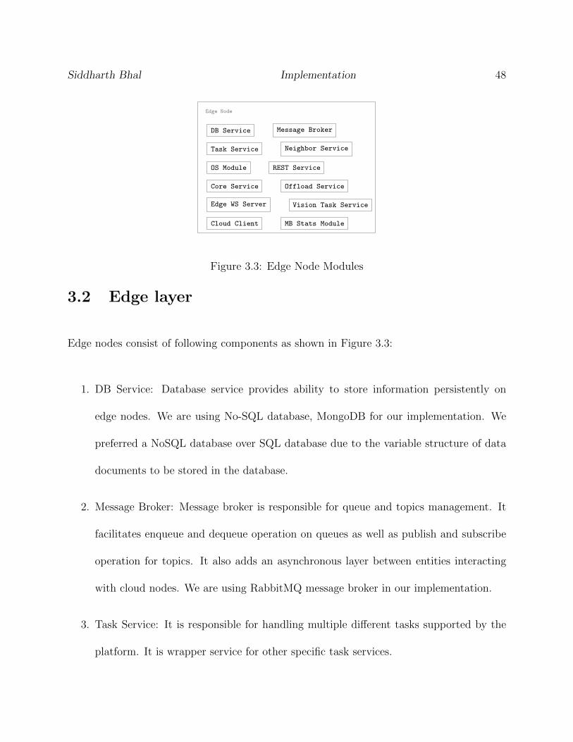
3.2 Edge layer
Edge nodes consist of following components as shown in Figure 3.3:
1. DB Service: Database service provides ability to store information persistently on
edge nodes. We are using No-SQL database, MongoDB for our implementation. We
preferred a NoSQL database over SQL database due to the variable structure of data
documents to be stored in the database.
2. Message Broker: Message broker is responsible for queue and topics management. It
facilitates enqueue and dequeue operation on queues as well as publish and subscribe
operation for topics. It also adds an asynchronous layer between entities interacting
with cloud nodes. We are using RabbitMQ message broker in our implementation.
3. Task Service: It is responsible for handling multiple different tasks supported by the
platform. It is wrapper service for other specific task services.
Siddharth Bhal Implementation 49
:Edge Node :Cloud Message Broker :Cloud Node
connectWebSocketwebSocketResponse
init Request
init Done Rsp
register Services
service Registration Done
get Neighbors
get Neighbors Done
subscribe Topics osenv
Req enqueue UUID
Figure 3.4: Edge Cloud Sequence Diagram
4. OS Modules: This module is responsible for getting OS monitoring variables like cur-
rent CPU usage, CPU idle time, free memory.
5. MB Stats Module: Message broker statistics module is used to monitor statistics of
queues and topics in running message broker instance.
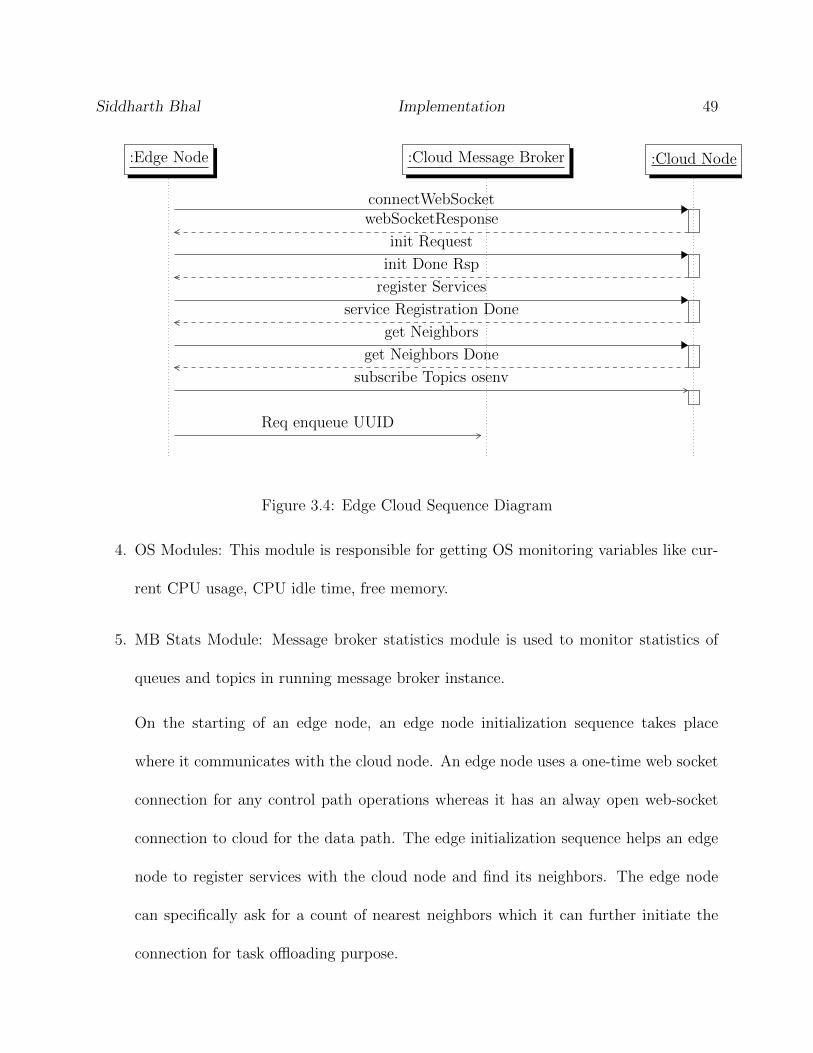
On the starting of an edge node, an edge node initialization sequence takes place
where it communicates with the cloud node. An edge node uses a one-time web socket
connection for any control path operations whereas it has an alway open web-socket
connection to cloud for the data path. The edge initialization sequence helps an edge
node to register services with the cloud node and find its neighbors. The edge node
can specifically ask for a count of nearest neighbors which it can further initiate the
connection for task offloading purpose.
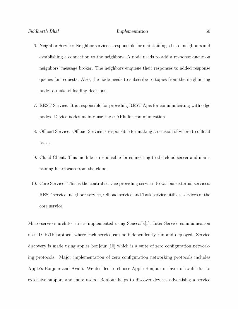
Siddharth Bhal Implementation 50
6. Neighbor Service: Neighbor service is responsible for maintaining a list of neighbors and
establishing a connection to the neighbors. A node needs to add a response queue on
neighbors’ message broker. The neighbors enqueue their responses to added response
queues for requests. Also, the node needs to subscribe to topics from the neighboring
node to make offloading decisions.
7. REST Service: It is responsible for providing REST Apis for communicating with edge
nodes. Device nodes mainly use these APIs for communication.
8. Offload Service: Offload Service is responsible for making a decision of where to offload
tasks.
9. Cloud Client: This module is responsible for connecting to the cloud server and main-
taining heartbeats from the cloud.
10. Core Service: This is the central service providing services to various external services.
REST service, neighbor service, Offload service and Task service utilizes services of the
core service.
Micro-services architecture is implemented using SenecaJs[1]. Inter-Service communication
uses TCP/IP protocol where each service can be independently run and deployed. Service
discovery is made using apples bonjour [16] which is a suite of zero configuration network-
ing protocols. Major implementation of zero configuration networking protocols includes
Apple’s Bonjour and Avahi. We decided to choose Apple Bonjour in favor of avahi due to
extensive support and more users. Bonjour helps to discover devices advertising a service
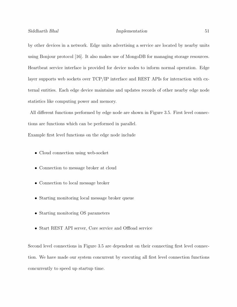
Siddharth Bhal Implementation 51
by other devices in a network. Edge units advertising a service are located by nearby units
using Bonjour protocol [16]. It also makes use of MongoDB for managing storage resources.
Heartbeat service interface is provided for device nodes to inform normal operation. Edge
layer supports web sockets over TCP/IP interface and REST APIs for interaction with ex-
ternal entities. Each edge device maintains and updates records of other nearby edge node
statistics like computing power and memory.
All different functions performed by edge node are shown in Figure 3.5. First level connec-
tions are functions which can be performed in parallel.
Example first level functions on the edge node include
• Cloud connection using web-socket
• Connection to message broker at cloud
• Connection to local message broker
• Starting monitoring local message broker queue
• Starting monitoring OS parameters
• Start REST API server, Core service and Offload service
Second level connections in Figure 3.5 are dependent on their connecting first level connec-
tion. We have made our system concurrent by executing all first level connection functions
concurrently to speed up startup time.
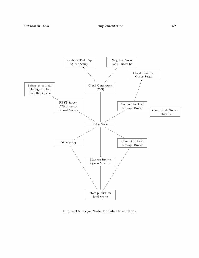
Siddharth Bhal Implementation 52
Edge Node
OS Monitor
Message BrokerQueue Monitor
start publish onlocal topics
Connect to localMessage Broker
Connect to cloudMessage Broker
Cloud Node TopicsSubscribe
Cloud Task RspQueue Setup
Cloud Connection(WS)
Neighbor NodeTopic Subscribe
Neighbor Task RspQueue Setup
REST Server,CORE service,Offload Service
Subscribe to localMessage BrokerTask Req Queue
Figure 3.5: Edge Node Module Dependency
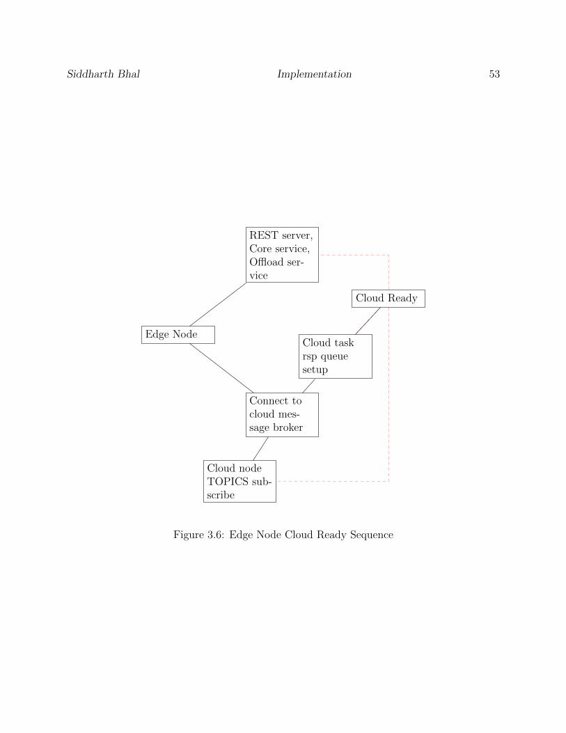
Siddharth Bhal Implementation 53
Edge Node
Connect tocloud mes-sage broker
Cloud nodeTOPICS sub-scribe
Cloud taskrsp queuesetup
Cloud Ready
REST server,Core service,Offload ser-vice
Figure 3.6: Edge Node Cloud Ready Sequence
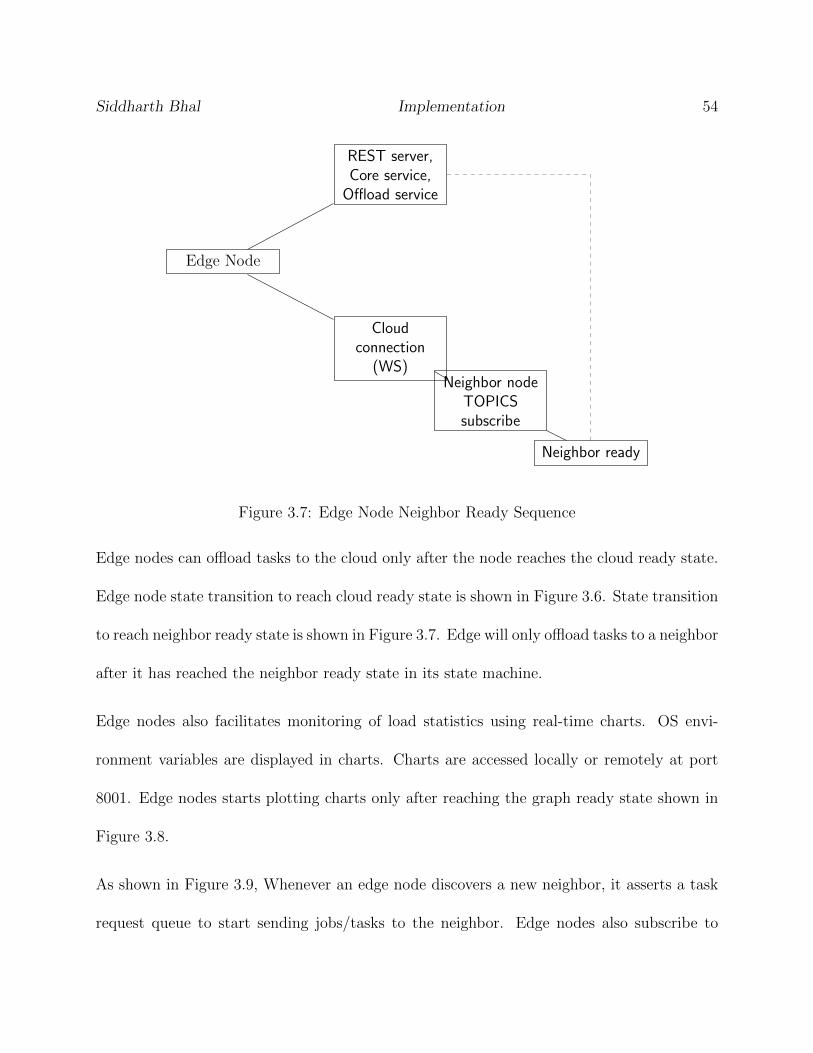
Siddharth Bhal Implementation 54
Edge Node
Cloudconnection
(WS)Neighbor node
TOPICSsubscribe
Neighbor ready
REST server,Core service,
Offload service
Figure 3.7: Edge Node Neighbor Ready Sequence
Edge nodes can offload tasks to the cloud only after the node reaches the cloud ready state.
Edge node state transition to reach cloud ready state is shown in Figure 3.6. State transition
to reach neighbor ready state is shown in Figure 3.7. Edge will only offload tasks to a neighbor
after it has reached the neighbor ready state in its state machine.
Edge nodes also facilitates monitoring of load statistics using real-time charts. OS envi-
ronment variables are displayed in charts. Charts are accessed locally or remotely at port
8001. Edge nodes starts plotting charts only after reaching the graph ready state shown in
Figure 3.8.
As shown in Figure 3.9, Whenever an edge node discovers a new neighbor, it asserts a task
request queue to start sending jobs/tasks to the neighbor. Edge nodes also subscribe to
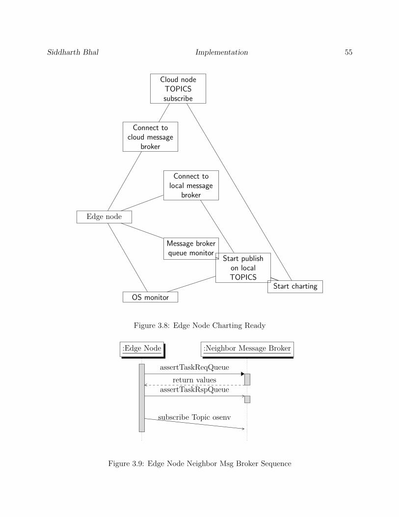
Siddharth Bhal Implementation 55
Edge node
OS monitor
Message brokerqueue monitor
Start publishon localTOPICS
Start charting
Connect tolocal message
broker
Connect tocloud message
broker
Cloud nodeTOPICSsubscribe
Figure 3.8: Edge Node Charting Ready
:Edge Node :Neighbor Message Broker
assertTaskReqQueue
return valuesassertTaskRspQueue
subscribe Topic osenv
Figure 3.9: Edge Node Neighbor Msg Broker Sequence
Siddharth Bhal Implementation 56
published topics from neighboring nodes, which are used to make offloading decisions.
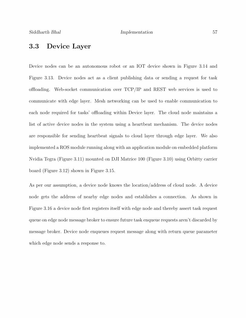
Siddharth Bhal Implementation 57
3.3 Device Layer
Device nodes can be an autonomous robot or an IOT device shown in Figure 3.14 and
Figure 3.13. Device nodes act as a client publishing data or sending a request for task
offloading. Web-socket communication over TCP/IP and REST web services is used to
communicate with edge layer. Mesh networking can be used to enable communication to
each node required for tasks’ offloading within Device layer. The cloud node maintains a
list of active device nodes in the system using a heartbeat mechanism. The device nodes
are responsible for sending heartbeat signals to cloud layer through edge layer. We also
implemented a ROS module running along with an application module on embedded platform
Nvidia Tegra (Figure 3.11) mounted on DJI Matrice 100 (Figure 3.10) using Orbitty carrier
board (Figure 3.12) shown in Figure 3.15.
As per our assumption, a device node knows the location/address of cloud node. A device
node gets the address of nearby edge nodes and establishes a connection. As shown in
Figure 3.16 a device node first registers itself with edge node and thereby assert task request
queue on edge node message broker to ensure future task enqueue requests aren’t discarded by
message broker. Device node enqueues request message along with return queue parameter
which edge node sends a response to.
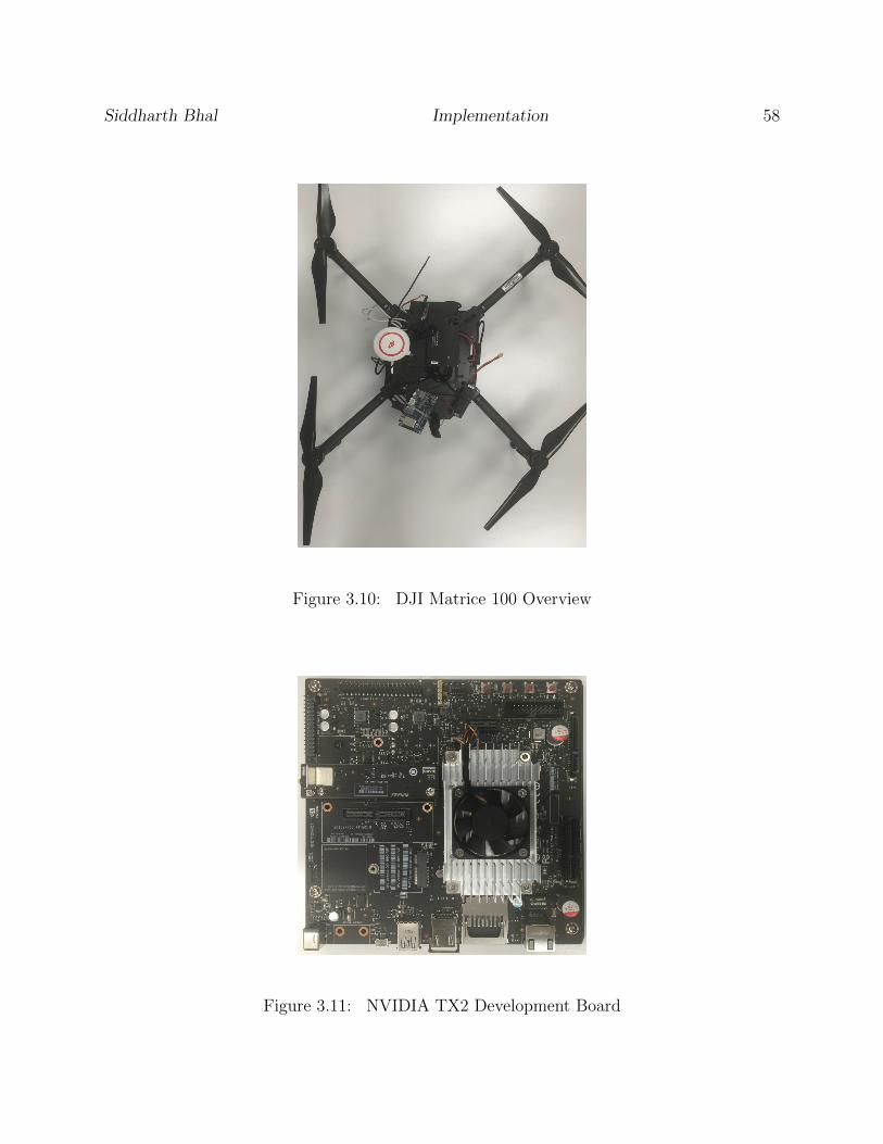
Siddharth Bhal Implementation 58
Figure 3.10: DJI Matrice 100 Overview
Figure 3.11: NVIDIA TX2 Development Board
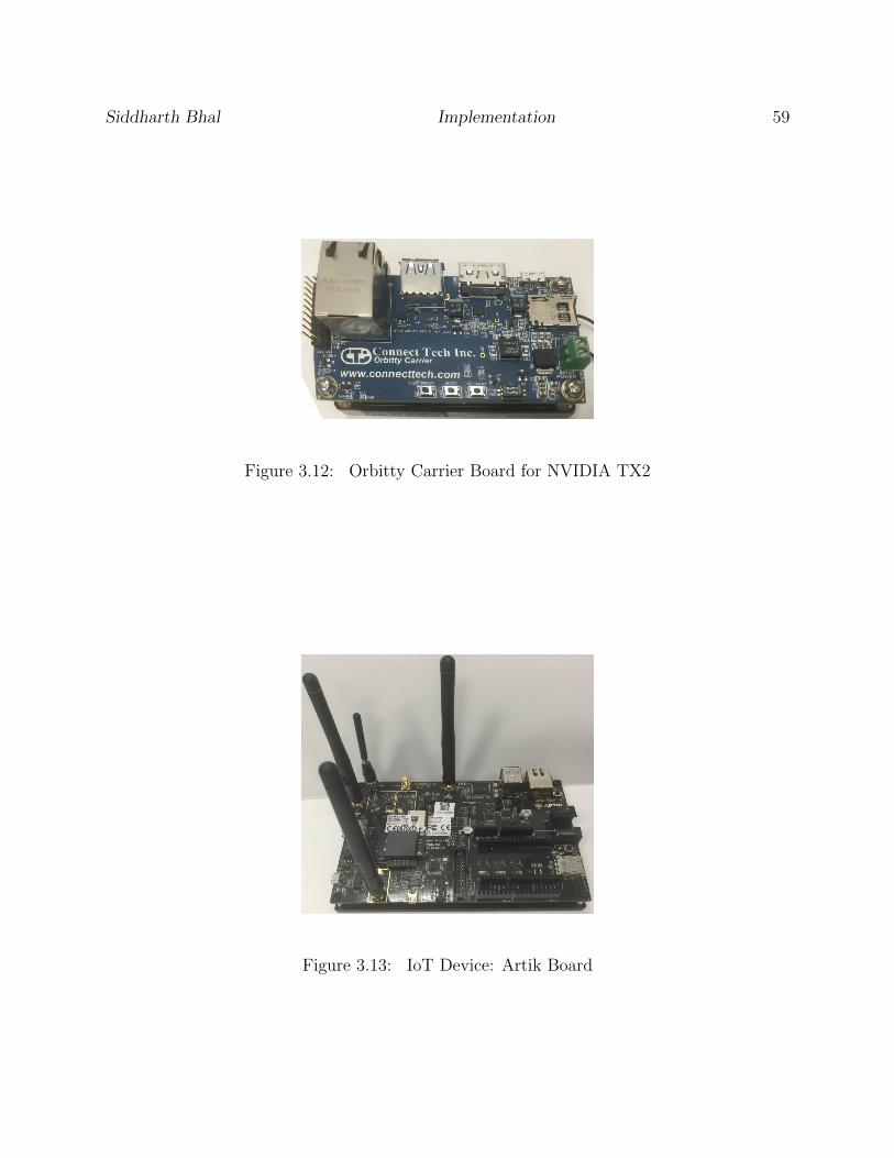
Siddharth Bhal Implementation 59
Figure 3.12: Orbitty Carrier Board for NVIDIA TX2
Figure 3.13: IoT Device: Artik Board
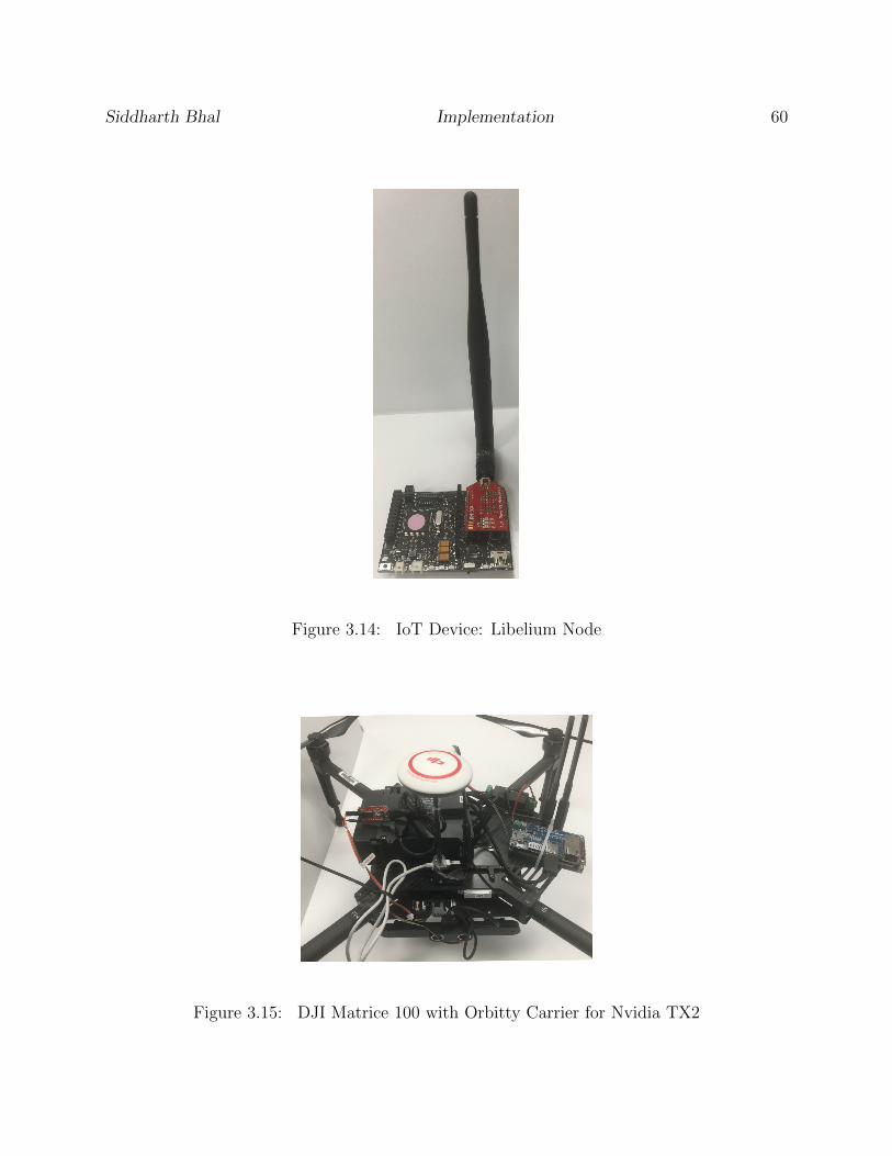
Siddharth Bhal Implementation 60
Figure 3.14: IoT Device: Libelium Node
Figure 3.15: DJI Matrice 100 with Orbitty Carrier for Nvidia TX2
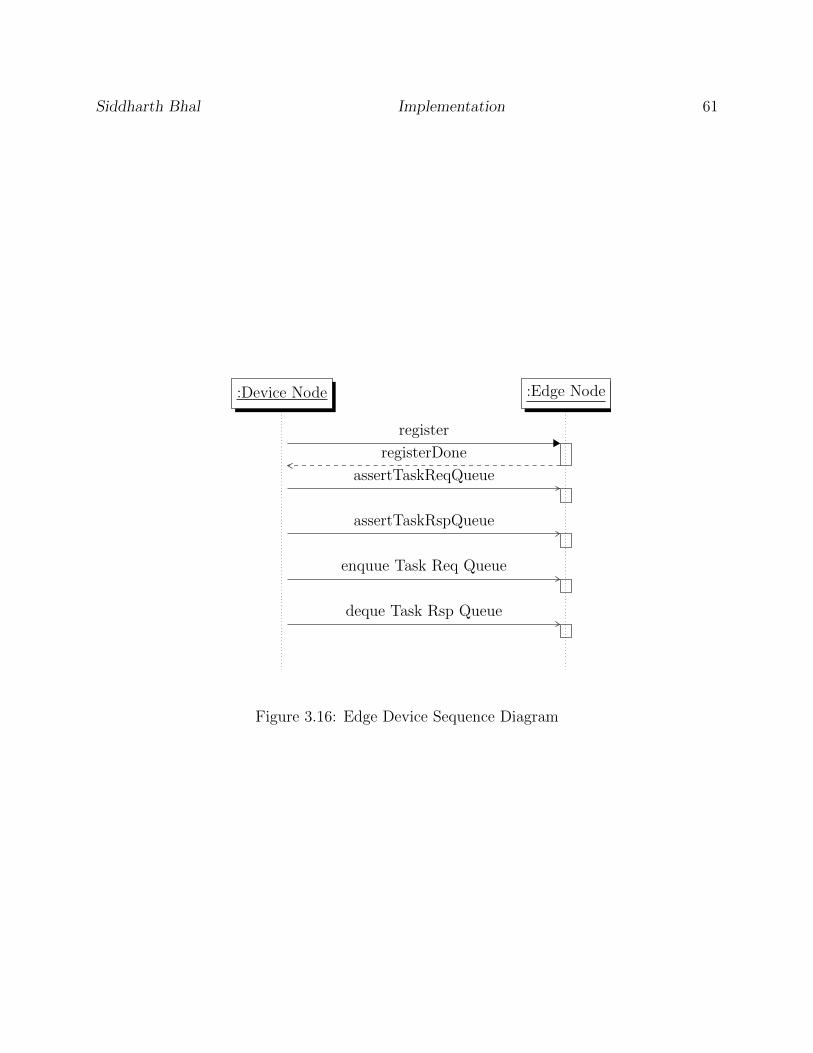
Siddharth Bhal Implementation 61
:Device Node :Edge Node
register
registerDone
assertTaskReqQueue
assertTaskRspQueue
enquue Task Req Queue
deque Task Rsp Queue
Figure 3.16: Edge Device Sequence Diagram
Chapter 4
Task Allocation
In this chapter, we will discuss various task allocation algorithms suitable for our architecture.
We will start with classical multi-criteria decision making (MCDM) algorithms like TOPSIS
& TODIM. MCDM algorithms evaluate multiple criteria for making a decision when choosing
the best alternative. Conflicting criteria can make a problem more complicated but may
lead to better decisions. We will also talk about ways of improving the performance of the
algorithms using model-free reinforcement learning technique called Q-learning.
4.1 MCDM
Multi-criteria decision-making algorithms help users to select the best set of criteria to select
from alternatives.
62
Siddharth Bhal Task Allocation 63
Some of the characteristics for choosing criteria are:
• Completeness: Our criteria should represent a complete picture of the system.
• Redundancy: Chosen criteria should have least redundancy among each other.
• Operationality: We should be able to measure and compare alternatives based on
criteria precisely.
There are two types of criteria: min cost criteria and max benefit criteria. A smaller value of
min cost criteria favors an alternative whereas a higher value of max benefit criteria favors
an alternative. In most of MCDM algorithms, weights define the relative importance of
criteria in choosing alternatives. A decision matrix is a consolidated view of criteria and
their weights which help us to make an objective decision.
4.2 TOPSIS
TOPSIS is Technique for Order of Preference by Similarity to Ideal Solution which is a multi-
criteria decision analysis method. This method can be used to compare various alternatives
based on criteria and weights given to the criteria. One of the assumptions on criteria is that
they are monotonically increasing. In this method, a Positive ideal alternative and Negative
ideal alternative are deduced. The algorithm finds the alternative which is closest to ideal
positive alternative and farthest from the negative ideal alternative.
Steps for choosing best alternative are listed below:
Siddharth Bhal Task Allocation 64
• Step 1: Establish an evaluation matrix X with m alternatives and n criteria.
X = (xij)mxn (4.1)
• Step 2: Normalize performance matrix X from Equation 4.1 w.r.t criteria
N = (nij)m∗n, wherenij =xij√∑mi=1 x
2ij
, i = 1, ...,m, j = 1, ..., n (4.2)
Consequently, each criteria for alternatives are on same scale.
• Step 3: Calculate the weighted normalized decision matrix
tij = nij ∗ wj, i = 1, 2..m, j = 1, 2...ntij = wj ⊗ nij, j = 1, ..., n, i = 1, ...,m (4.3)
• Step 4: Determine worst alternative A− and best alternative A+
A+ = v+1 , ...., v+n = {(max
ivij, jεJ+)(min
ivij, jεJ−)}
i = 1, ...,m
(4.4)
A− = v−1 , ...., v−n = {(min
ivij, jεJ+)(max
ivij, jεJ−)}
i = 1, ...,m
(4.5)
where,
J+ = {j = 1, ..., n|jε criteria having positive impact and ,
J− = {j = 1, ..., n|jε criteria having negative impact
• Step 5: Calculate the separation measure by L2 distance between alternative i and
worst condition A−
Siddharth Bhal Task Allocation 65
The separation of an alternative from position ideal solution is
d+i =
√√√√ n∑j=1
(vij − v+j )2, i = 1, ...,m (4.6)
The separation of an alternative from negative ideal solution is
d−i =
√√√√ n∑j=1
(vij − v−j )2, i = 1, ...,m (4.7)
• Step 6: Calculate the relative closeness to worst condition
Ri =d−i
d+i + d−i, i = 1, ...m (4.8)
If Ri == 1 if and only if alternative i has best condition
If Ri == 0 if and only if alternative i has worst condition
• Step 7: Rank the alternative in preference order
Rank the best alternatives according to relative closeness to worst condition in de-
creasing order.
4.3 TODIM
TODIM is an acronym in Portuguese for Interactive and Multi-criteria Decision Making. It
is a multi-criteria decision-making algorithm. This algorithm is based on Prospect Theory
[37]. TODIM is different from other multi-criteria decision-making algorithms in the respect
that it doesn’t globally try to increase the target value at the maximum possible rate. It
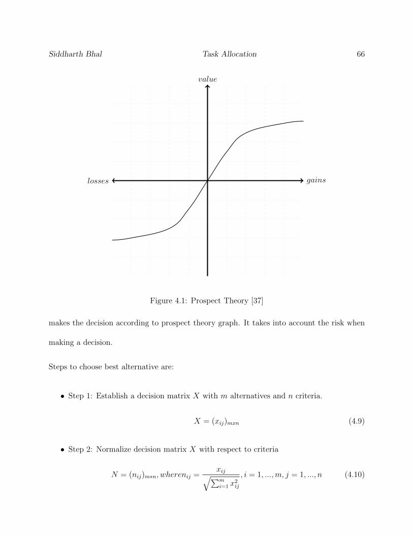
Siddharth Bhal Task Allocation 66
gains
value
losses
Figure 4.1: Prospect Theory [37]
makes the decision according to prospect theory graph. It takes into account the risk when
making a decision.
Steps to choose best alternative are:
• Step 1: Establish a decision matrix X with m alternatives and n criteria.
X = (xij)mxn (4.9)
• Step 2: Normalize decision matrix X with respect to criteria
N = (nij)m∗n, wherenij =xij√∑mi=1 x
2ij
, i = 1, ...,m, j = 1, ..., n (4.10)
Siddharth Bhal Task Allocation 67
Consequently, each criteria for alternatives are on same scale.
• Step 3: Calculate dominance of Ai over each alternative Aj
δ(Ai, Aj) =n∑c=1
φc(Ai, Aj),∀(i, j) (4.11)
where,
φc(Ai, Aj) =
√wrc∑c wrc
d(sic, sjc), if d(sic, sjc) ≥ 0
0, if d(sic, sjc) = 0
−1θ
√∑c wrc
wrcd(sic, sjc), if d(sic, sjc) ≤ 0
(4.12)
• Step 4: The global multiattribute value
εi =
∑j δ(Ai, Aj)−mini
∑j δ(Ai, Aj)
maxi∑
j δ(Ai, Aj)−mini∑
j δ(Ai, Aj)(4.13)
• Step 5: Sort the alternatives according to εi
A+ = v+1 , ...., v+n = {(max
ivij, jεJ+)(min
ivij, jεJ−)} (4.14)
i = 1, ...,m (4.15)
A− = v−1 , ...., v−n = {(min
ivij, jεJ+)(max
ivij, jεJ−)} (4.16)
i = 1, ...,m (4.17)
TODIM algorithm is very similar to TOPSIS with a difference of values function. TOPSIS
has a linear valued function whereas TODIM has “S” curve valued function shown in Fig-
ure 4.1. Due to “S” curve valued function, TODIM limits the rate of increase in gains as
well as limits the rate of increase of losses.
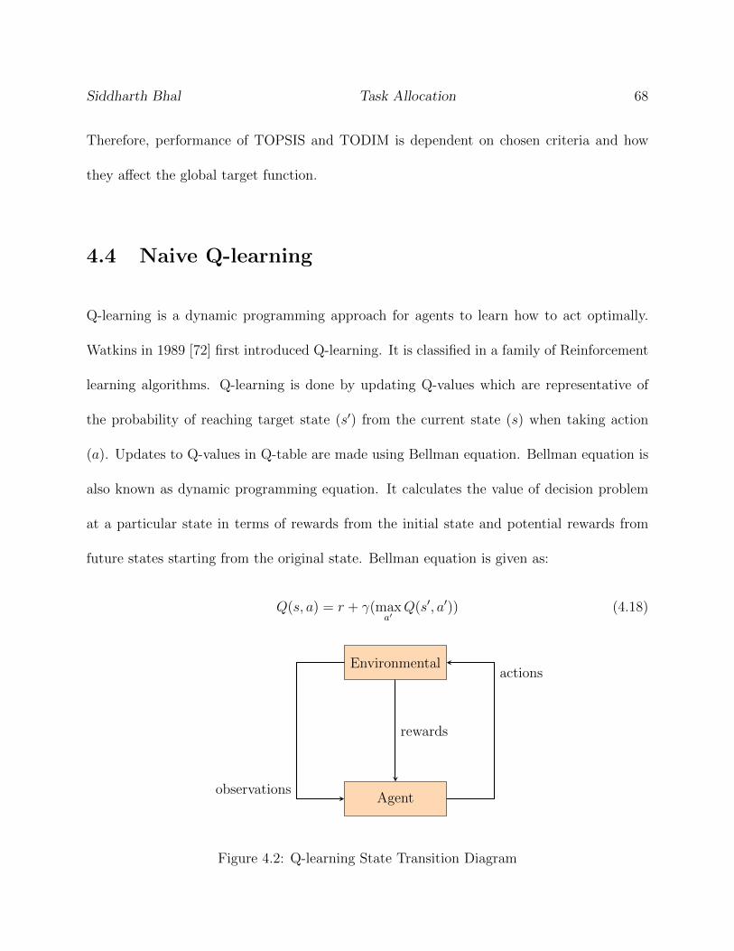
Siddharth Bhal Task Allocation 68
Therefore, performance of TOPSIS and TODIM is dependent on chosen criteria and how
they affect the global target function.
4.4 Naive Q-learning
Q-learning is a dynamic programming approach for agents to learn how to act optimally.
Watkins in 1989 [72] first introduced Q-learning. It is classified in a family of Reinforcement
learning algorithms. Q-learning is done by updating Q-values which are representative of
the probability of reaching target state (s′) from the current state (s) when taking action
(a). Updates to Q-values in Q-table are made using Bellman equation. Bellman equation is
also known as dynamic programming equation. It calculates the value of decision problem
at a particular state in terms of rewards from the initial state and potential rewards from
future states starting from the original state. Bellman equation is given as:
Q(s, a) = r + γ(maxa′
Q(s′, a′)) (4.18)
Environmental
Agentobservations
actions
rewards
Figure 4.2: Q-learning State Transition Diagram
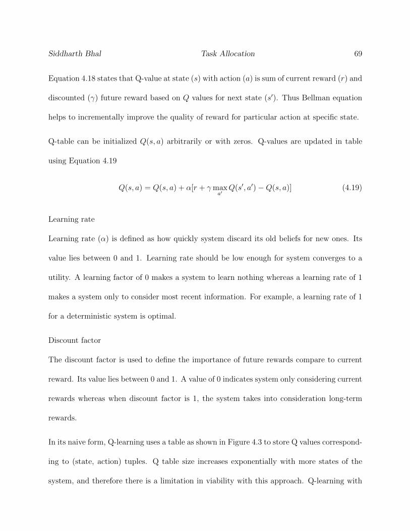
Siddharth Bhal Task Allocation 69
Equation 4.18 states that Q-value at state (s) with action (a) is sum of current reward (r) and
discounted (γ) future reward based on Q values for next state (s′). Thus Bellman equation
helps to incrementally improve the quality of reward for particular action at specific state.
Q-table can be initialized Q(s, a) arbitrarily or with zeros. Q-values are updated in table
using Equation 4.19
Q(s, a) = Q(s, a) + α[r + γmaxa′
Q(s′, a′)−Q(s, a)] (4.19)
Learning rate
Learning rate (α) is defined as how quickly system discard its old beliefs for new ones. Its
value lies between 0 and 1. Learning rate should be low enough for system converges to a
utility. A learning factor of 0 makes a system to learn nothing whereas a learning rate of 1
makes a system only to consider most recent information. For example, a learning rate of 1
for a deterministic system is optimal.
Discount factor
The discount factor is used to define the importance of future rewards compare to current
reward. Its value lies between 0 and 1. A value of 0 indicates system only considering current
rewards whereas when discount factor is 1, the system takes into consideration long-term
rewards.
In its naive form, Q-learning uses a table as shown in Figure 4.3 to store Q values correspond-
ing to (state, action) tuples. Q table size increases exponentially with more states of the
system, and therefore there is a limitation in viability with this approach. Q-learning with
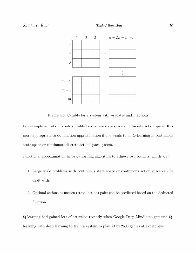
Siddharth Bhal Task Allocation 70
1 2 3 n− 2n− 1 n
1
2
3
m− 2
m− 1
m
· · ·
· · ·
......
. . .
Figure 4.3: Q-table for a system with m states and n actions
tables implementation is only suitable for discrete state space and discrete action space. It is
more appropriate to do function approximation if one wants to do Q-learning in continuous
state space or continuous discrete action space system.
Functional approximation helps Q-learning algorithm to achieve two benefits, which are:
1. Large scale problems with continuous state space or continuous action space can be
dealt with.
2. Optimal actions at unseen (state, action) pairs can be predicted based on the deducted
function
Q-learning had gained lots of attention recently when Google Deep Mind amalgamated Q-
learning with deep learning to train a system to play Atari 2600 games at expert level.
Siddharth Bhal Task Allocation 71
4.4.1 Q learning with TOPSIS
As defined in section 4.2 TOPSIS algorithm chooses the best alternative out of alternatives
based on the closeness to the positive ideal solution (PIS) and separation from negative ideal
solution(NIS). TOPSIS algorithm works great for a static system for which optimal criteria
weights can be predetermined. To make it dynamic, we can use Q-learning to update weights
on criteria in real-time based on rewards output of the system. Applying Q-learning this
way has following benefits:
1. Weights can be discretized and thus reducing the problem size to much smaller scale.
2. Discretizing criteria weights also helps to produce prediction faster due to fast process-
ing and less memory requirement.
Steps to discretize state space for task allocation problem are:
Step 1: Discretize criteria weights into parts. Since weight per criteria belongs to (0,1].
wit = 0.1 ∗ x, x = 0, 1..., 10, i = 1, ...,m (4.20)
Therefore, the number of different weight values each weight variable in weight vector can
have is 11.
Siddharth Bhal Task Allocation 72
Step 2: Discretize actions in steps of criteria weights increments /decrements.
at =
wit + 0.1
wit
wit − 0.1
∀i = 1..,m (4.21)
Rows of the Q matrix represent the various state a system can achieve. The number of rows
in the Q matrix will be 11m. The number of columns is equal to the number of different
actions a system can take at a particular point in time. Here is the Q state transition for
system with m criteria
(w1t, ...., wmt) =⇒ (a1t, ...., amt) =⇒ (w1t+1, ...., wmt+1) (4.22)
An action providing most rewards at a system state is one with highest Q-value among all
actions at the state.
4.4.2 Q learning with TODIM
Similar to Q-learning with TOPSIS approach, weights for each criterion are discretized in
steps of 0.1 as shown in Equation 4.20 and optimal weights are learned using Q-learning.
The number of different weight values each weight variable in weight vector can have is 11.
Equation 4.21 gives different actions that can be taken at each state
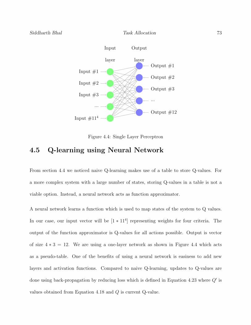
Siddharth Bhal Task Allocation 73
Input #1
Input #2
Input #3
...
Input #114
Output #1
Output #2
Output #3
...
Output #12
Output
layer
Input
layer
Figure 4.4: Single Layer Perceptron
4.5 Q-learning using Neural Network
From section 4.4 we noticed naive Q-learning makes use of a table to store Q-values. For
a more complex system with a large number of states, storing Q-values in a table is not a
viable option. Instead, a neural network acts as function approximator.
A neural network learns a function which is used to map states of the system to Q values.
In our case, our input vector will be [1 ∗ 114] representing weights for four criteria. The
output of the function approximator is Q-values for all actions possible. Output is vector
of size 4 ∗ 3 = 12. We are using a one-layer network as shown in Figure 4.4 which acts
as a pseudo-table. One of the benefits of using a neural network is easiness to add new
layers and activation functions. Compared to naive Q-learning, updates to Q-values are
done using back-propagation by reducing loss which is defined in Equation 4.23 where Q′ is
values obtained from Equation 4.18 and Q is current Q-value.

Siddharth Bhal Task Allocation 74
Loss =∑
(Q′ −Q)2 (4.23)
Q-learning with functional approximation helps to deal with the limitation of discrete state
space and discrete action space. A functional approach also helps in prediction of unexplored
state-action pairs.
The Single layer perceptron in Figure 4.4 can only learn a linear function which is suitable
for our linear system.
We made use of TensorFlow [2] to implement our neural network.
4.5.1 Q learning with TOPSIS using Neural Network
In this approach we use TOPSIS algorithm as mentioned in section 4.2 with Q-learning using
Neural Network. Weights used in TOPSIS for criteria are discretized as follows:
Step 1: Discretize weights into parts. Since weight per criteria belongs to (0,1].
wit = 0.1 ∗ x, x = 0, 1..., 10, i = 1, ...,m (4.24)
Therefore, the number of different weight values each weight variable in weight vector can
have is 11.
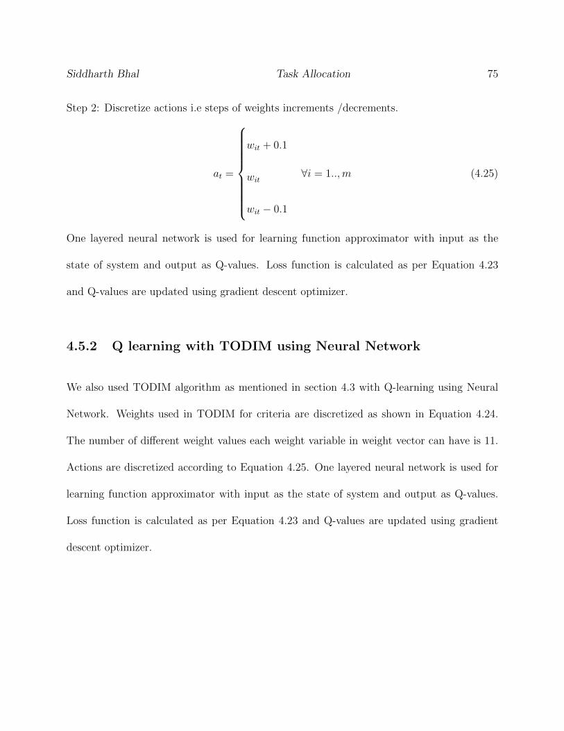
Siddharth Bhal Task Allocation 75
Step 2: Discretize actions i.e steps of weights increments /decrements.
at =
wit + 0.1
wit
wit − 0.1
∀i = 1..,m (4.25)
One layered neural network is used for learning function approximator with input as the
state of system and output as Q-values. Loss function is calculated as per Equation 4.23
and Q-values are updated using gradient descent optimizer.
4.5.2 Q learning with TODIM using Neural Network
We also used TODIM algorithm as mentioned in section 4.3 with Q-learning using Neural
Network. Weights used in TODIM for criteria are discretized as shown in Equation 4.24.
The number of different weight values each weight variable in weight vector can have is 11.
Actions are discretized according to Equation 4.25. One layered neural network is used for
learning function approximator with input as the state of system and output as Q-values.
Loss function is calculated as per Equation 4.23 and Q-values are updated using gradient
descent optimizer.
Chapter 5
Results
In this chapter, we compare the performance of different task allocation algorithms for overall
system latency. We discuss the experimentation setup and selection of nodes at each layer to
represent a heterogeneous multi-robot system interacting with IOT. We further discuss the
significant load indicators used in each task allocation algorithm and list the fixed parameters
used in each algorithm.
5.1 Experimentation Setup
The experimentation setup consists of 3 edge Nodes with a single cloud node as shown in
Figure 5.1. Hardware components used are shown in Figure 5.2
76
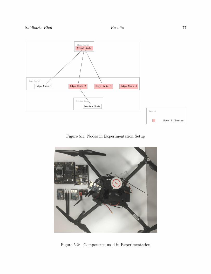
Siddharth Bhal Results 77
Edge Layer
Edge Node 1 Edge Node 2 Edge Node 3 Edge Node 4
Cloud Layer
Cloud Node
Device Layer
Device Node
Legend
Node 2 Cluster
Figure 5.1: Nodes in Experimentation Setup
Figure 5.2: Components used in Experimentation
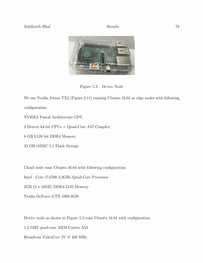
Siddharth Bhal Results 78
Figure 5.3: Device Node
We use Nvidia Jetson TX2 (Figure 3.11) running Ubuntu 16.04 as edge nodes with following
configuration:
NVIDIA Pascal Architecture GPU
2 Denver 64-bit CPUs + Quad-Core A57 Complex
8 GB L128 bit DDR4 Memory
32 GB eMMC 5.1 Flash Storage
Cloud node runs Ubuntu 16.04 with following configuration:
Intel - Core i7-6700 3.4GHz Quad-Core Processor
2GB (2 x 16GB) DDR4-2133 Memory
Nvidia GeForce GTX 1060 6GB
Device node as shown in Figure 5.3 runs Ubuntu 16.04 with configuration:
1.2 GHZ quad-core ARM Cortex A53
Broadcom VideoCore IV @ 400 MHz

Siddharth Bhal Results 79
1 GB LPDDR2-900 SDRAM
Heterogeneous devices are chosen to represent a heterogeneous autonomous network.
Performance indicators used as criteria in algorithms are:
• CPU Utilization: It represents amount of work handled by CPU. A low value of CPU
Utilization represents percentage of free processing resources available at a node for
doing the computation.
• Free Memory: It shows the percentage of free memory available for usage.
• Number of Active current contexts: It shows the number of active tasks handled at a
node currently.
• Backlog of Messages in Message Broker: It shows the number of messages ready to be
processed in ready queue of the message broker.
There are three types of tasks which can be used to gauge the performance of algorithms:
1. Real-time Task (RT)
For the real-time task, I am doing optical character recognition from image dataset.
2. Stress Task (ST)
Here I am using a stress-ng program to do bogus CPU cycles. This task is mainly used
to see the behavior of algorithm under high CPU load.
Siddharth Bhal Results 80
3. Dummy Task (DT)
Dummy Task will simply do idle wait for some time before responding. Dummy task
helps to gauge algorithm precision as no impact is there when CPU utilization is low.
We found Stress Task (ST) as the most precise measurement for comparing algorithms due
to fixed amount of resource requirement per task. We found consistent results with ST. One
of the reasons for inconsistency with real-time task can be attributed to different resource
requirement for each job which is part of a task. It makes it challenging to compare and
benchmark task allocation algorithms. Due to this observation, we decided to only conduct
experiments with Stress task (ST) although we have successfully tested the system with
balancing of image recognition tasks.
The multi criteria decision making algorithms make use of criteria to make the decision of
choosing the best alternative. In our system, each alternative is a node where the task can
be scheduled. Therefore each node is required to provides all criteria values required to make
a decision by task allocation algorithm.
We used following criteria to making offloading decision to optimize latency:
• CPU Utilization
• Free Memory
• Number of Active Job Contexts
• Job Processing time
Siddharth Bhal Results 81
• Distance of target node
A Stress task with 90 CPU operation per job is scheduled at an interval of 1 job/sec at Edge
Node 2 in Figure 5.1. All CPU operations are bound on CPU1 of each node. This provides
a uniform scale for measuring systems latency for all algorithms. A device node releases jobs
at the rate of 1 job/sec and continues doing for an interval of 240sec.
5.2 Fixed Parameters
Fixed parameters used for each algorithm are shown in Table 5.1.
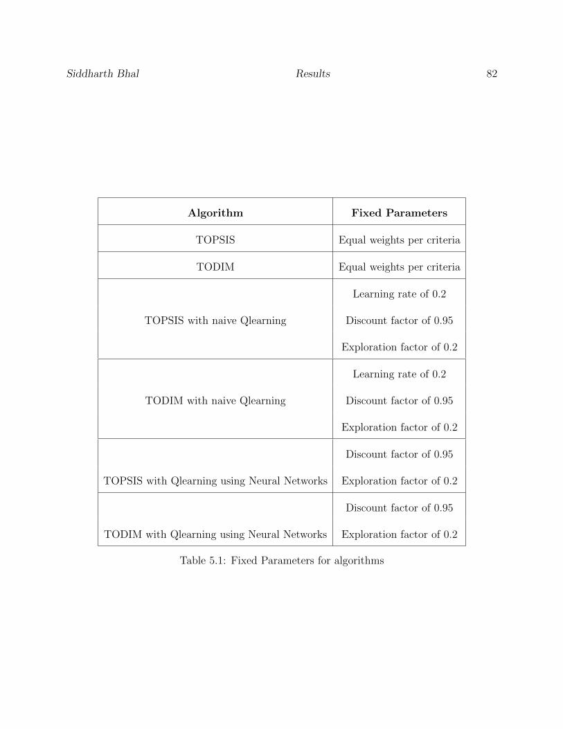
Siddharth Bhal Results 82
Algorithm Fixed Parameters
TOPSIS Equal weights per criteria
TODIM Equal weights per criteria
TOPSIS with naive Qlearning
Learning rate of 0.2
Discount factor of 0.95
Exploration factor of 0.2
TODIM with naive Qlearning
Learning rate of 0.2
Discount factor of 0.95
Exploration factor of 0.2
TOPSIS with Qlearning using Neural Networks
Discount factor of 0.95
Exploration factor of 0.2
TODIM with Qlearning using Neural Networks
Discount factor of 0.95
Exploration factor of 0.2
Table 5.1: Fixed Parameters for algorithms
Siddharth Bhal Results 83
5.3 Results Analysis
Following sections will make use short notation for algorithm’s full names as shown in Ta-
ble 5.2.
We observed algorithms which are offloading most tasks to cloud node instead of neighboring
nodes performed better due to higher computing resources available at the cloud without
being much distance from device node.
As per Figure 5.4, random algorithm has highest CPU utilization on edge node.
CPU Utilization is one of the criteria used in offloading decision-making algorithm. Fig-
ure 5.4 shows the value of CPU utilization is highest for the random algorithm. This is
mainly due to the randomness of the random algorithm in assigning tasks without realizing
the benefits of cloud offloading. CPU Utilization is directly proportional to the number of
tasks executed locally on the node. As shown in Figure 5.8 least number of tasks are of-
Short Notation Algorithm’s Name
TOPSIS Qlearn TOPSIS with naive Q-learning
TOPSIS Qlearn NN TOPSIS with Q-learning using Neural Network
TODIM Qlearn TODIM with naive Q-learning
TODIM Qlearn NN TODIM with Q-learning using Neural Network
Table 5.2: Short Notation for Algorithms

Siddharth Bhal Results 84
0 20 40 60 80 100 120 140 160 180 200 220 240
0.18
0.2
0.22
0.24
0.26
0.28
0.3
0.32
0.34
Time(s)
CP
UU
tiliza
tion
Edge
Node
Random AlgorithmTopsis
Topsis QlearnTopsis Qlearn NN
TodimTodim Qlearn
Todim Qlearn NN
Figure 5.4: CPU Utilization of Edge Node during Stress Task
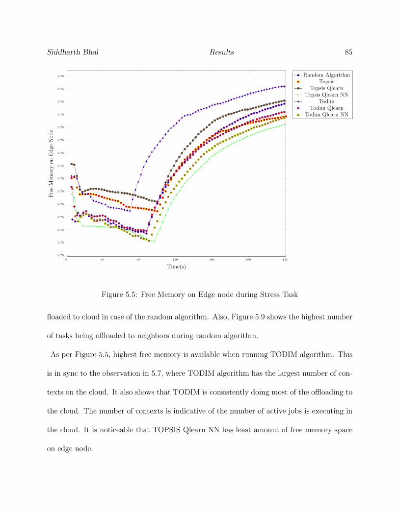
Siddharth Bhal Results 85
0 40 80 120 160 200 240
0.75
0.75
0.75
0.75
0.75
0.75
0.75
0.75
0.75
0.75
0.75
0.75
0.75
0.75
0.75
Time(s)
Fre
eM
emor
yon
Edge
Node
Random AlgorithmTopsis
Topsis QlearnTopsis Qlearn NN
TodimTodim Qlearn
Todim Qlearn NN
Figure 5.5: Free Memory on Edge node during Stress Task
floaded to cloud in case of the random algorithm. Also, Figure 5.9 shows the highest number
of tasks being offloaded to neighbors during random algorithm.
As per Figure 5.5, highest free memory is available when running TODIM algorithm. This
is in sync to the observation in 5.7, where TODIM algorithm has the largest number of con-
texts on the cloud. It also shows that TODIM is consistently doing most of the offloading to
the cloud. The number of contexts is indicative of the number of active jobs is executing in
the cloud. It is noticeable that TOPSIS Qlearn NN has least amount of free memory space
on edge node.
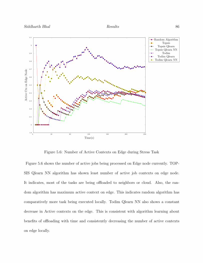
Siddharth Bhal Results 86
0 40 80 120 160 200 2401.9
2
2.1
2.2
2.3
2.4
2.5
2.6
2.7
2.8
2.9
3
3.1
Time(s)
Act
ive
Ctx
onE
dge
Nod
e
Random AlgorithmTopsis
Topsis QlearnTopsis Qlearn NN
TodimTodim Qlearn
Todim Qlearn NN
Figure 5.6: Number of Active Contexts on Edge during Stress Task
Figure 5.6 shows the number of active jobs being processed on Edge node currently. TOP-
SIS Qlearn NN algorithm has shown least number of active job contexts on edge node.
It indicates, most of the tasks are being offloaded to neighbors or cloud. Also, the ran-
dom algorithm has maximum active context on edge. This indicates random algorithm has
comparatively more task being executed locally. Todim Qlearn NN also shows a constant
decrease in Active contexts on the edge. This is consistent with algorithm learning about
benefits of offloading with time and consistently decreasing the number of active contexts
on edge locally.
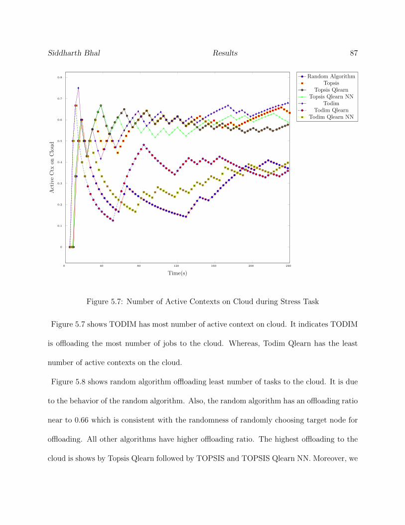
Siddharth Bhal Results 87
0 40 80 120 160 200 240
0
0.1
0.2
0.3
0.4
0.5
0.6
0.7
0.8
Time(s)
Act
ive
Ctx
onC
lou
d
Random AlgorithmTopsis
Topsis QlearnTopsis Qlearn NN
TodimTodim Qlearn
Todim Qlearn NN
Figure 5.7: Number of Active Contexts on Cloud during Stress Task
Figure 5.7 shows TODIM has most number of active context on cloud. It indicates TODIM
is offloading the most number of jobs to the cloud. Whereas, Todim Qlearn has the least
number of active contexts on the cloud.
Figure 5.8 shows random algorithm offloading least number of tasks to the cloud. It is due
to the behavior of the random algorithm. Also, the random algorithm has an offloading ratio
near to 0.66 which is consistent with the randomness of randomly choosing target node for
offloading. All other algorithms have higher offloading ratio. The highest offloading to the
cloud is shows by Topsis Qlearn followed by TOPSIS and TOPSIS Qlearn NN. Moreover, we
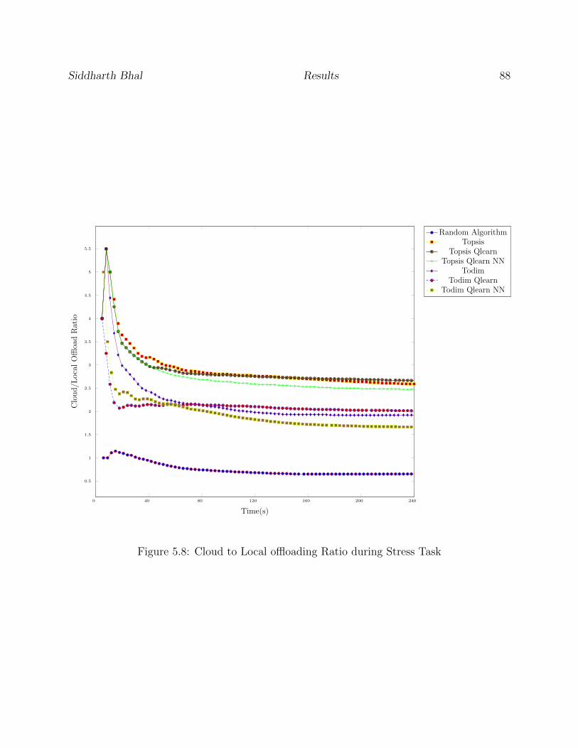
Siddharth Bhal Results 88
0 40 80 120 160 200 240
0.5
1
1.5
2
2.5
3
3.5
4
4.5
5
5.5
Time(s)
Clo
ud/L
oca
lO
ffloa
dR
atio
Random AlgorithmTopsis
Topsis QlearnTopsis Qlearn NN
TodimTodim Qlearn
Todim Qlearn NN
Figure 5.8: Cloud to Local offloading Ratio during Stress Task
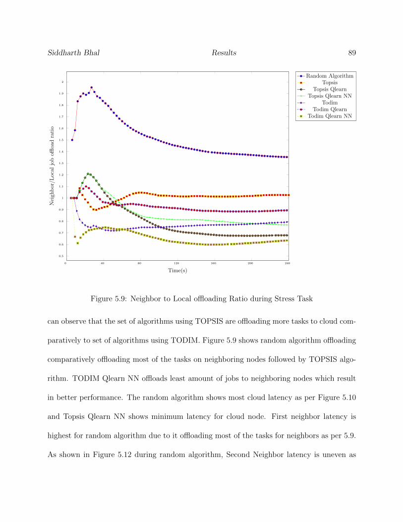
Siddharth Bhal Results 89
0 40 80 120 160 200 240
0.5
0.6
0.7
0.8
0.9
1
1.1
1.2
1.3
1.4
1.5
1.6
1.7
1.8
1.9
2
Time(s)
Nei
ghb
or/L
oca
ljo
boffl
oad
rati
o
Random AlgorithmTopsis
Topsis QlearnTopsis Qlearn NN
TodimTodim Qlearn
Todim Qlearn NN
Figure 5.9: Neighbor to Local offloading Ratio during Stress Task
can observe that the set of algorithms using TOPSIS are offloading more tasks to cloud com-
paratively to set of algorithms using TODIM. Figure 5.9 shows random algorithm offloading
comparatively offloading most of the tasks on neighboring nodes followed by TOPSIS algo-
rithm. TODIM Qlearn NN offloads least amount of jobs to neighboring nodes which result
in better performance. The random algorithm shows most cloud latency as per Figure 5.10
and Topsis Qlearn NN shows minimum latency for cloud node. First neighbor latency is
highest for random algorithm due to it offloading most of the tasks for neighbors as per 5.9.
As shown in Figure 5.12 during random algorithm, Second Neighbor latency is uneven as
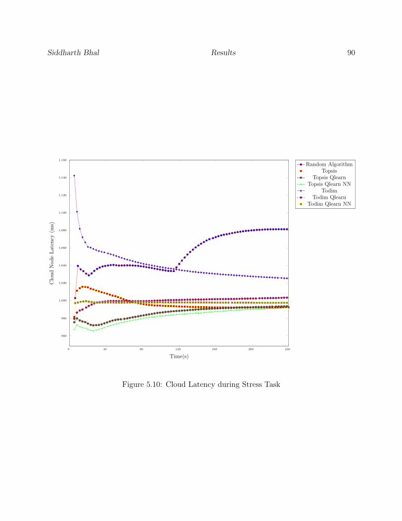
Siddharth Bhal Results 90
0 40 80 120 160 200 240
960
980
1,000
1,020
1,040
1,060
1,080
1,100
1,120
1,140
1,160
Time(s)
Clo
ud
Nod
eL
aten
cy(m
s)
Random AlgorithmTopsis
Topsis QlearnTopsis Qlearn NN
TodimTodim Qlearn
Todim Qlearn NN
Figure 5.10: Cloud Latency during Stress Task
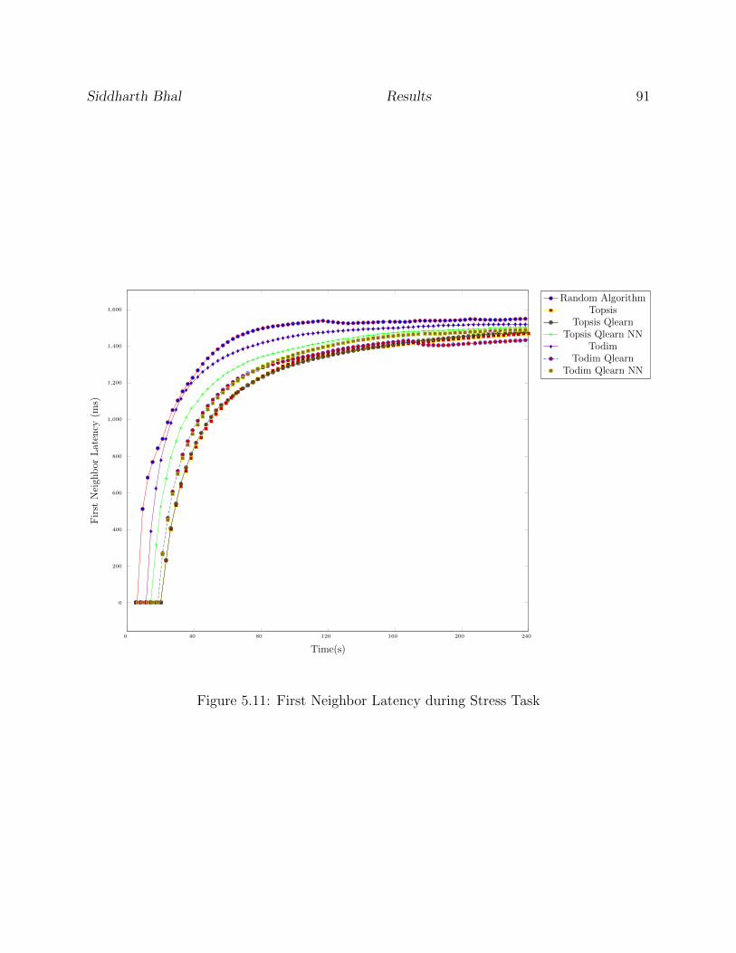
Siddharth Bhal Results 91
0 40 80 120 160 200 240
0
200
400
600
800
1,000
1,200
1,400
1,600
Time(s)
Fir
stN
eigh
bor
Lat
ency
(ms)
Random AlgorithmTopsis
Topsis QlearnTopsis Qlearn NN
TodimTodim Qlearn
Todim Qlearn NN
Figure 5.11: First Neighbor Latency during Stress Task

Siddharth Bhal Results 92
0 40 80 120 160 200 240
0
200
400
600
800
1,000
1,200
1,400
1,600
Time(s)
Fir
stN
eigh
bor
Lat
ency
(ms)
Random AlgorithmTopsis
Topsis QlearnTopsis Qlearn NN
TodimTodim Qlearn
Todim Qlearn NN
Figure 5.12: Second Neighbor Latency during Stress Task
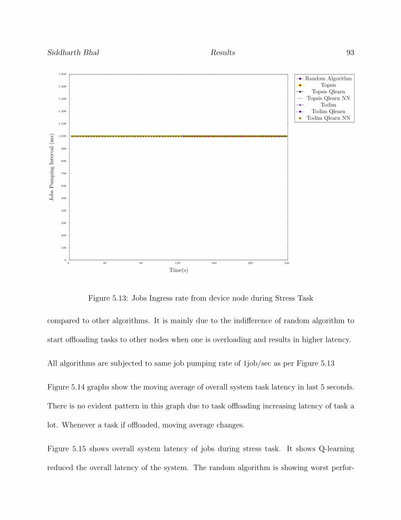
Siddharth Bhal Results 93
0 40 80 120 160 200 2400
100
200
300
400
500
600
700
800
900
1,000
1,100
1,200
1,300
1,400
1,500
Time(s)
Job
sP
um
pin
gIn
terv
al(m
s)
Random AlgorithmTopsis
Topsis QlearnTopsis Qlearn NN
TodimTodim Qlearn
Todim Qlearn NN
Figure 5.13: Jobs Ingress rate from device node during Stress Task
compared to other algorithms. It is mainly due to the indifference of random algorithm to
start offloading tasks to other nodes when one is overloading and results in higher latency.
All algorithms are subjected to same job pumping rate of 1job/sec as per Figure 5.13
Figure 5.14 graphs show the moving average of overall system task latency in last 5 seconds.
There is no evident pattern in this graph due to task offloading increasing latency of task a
lot. Whenever a task if offloaded, moving average changes.
Figure 5.15 shows overall system latency of jobs during stress task. It shows Q-learning
reduced the overall latency of the system. The random algorithm is showing worst perfor-
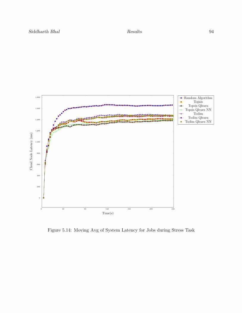
Siddharth Bhal Results 94
0 40 80 120 160 200 240
0
200
400
600
800
1,000
1,200
1,400
1,600
1,800
Time(s)
Clo
ud
Nod
eL
aten
cy(m
s)
Random AlgorithmTopsis
Topsis QlearnTopsis Qlearn NN
TodimTodim Qlearn
Todim Qlearn NN
Figure 5.14: Moving Avg of System Latency for Jobs during Stress Task
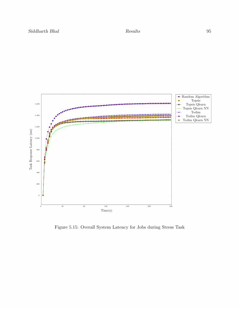
Siddharth Bhal Results 95
0 40 80 120 160 200 240
0
200
400
600
800
1,000
1,200
1,400
1,600
Time(s)
Tas
kR
esp
onse
Lat
ency
(ms)
Random AlgorithmTopsis
Topsis QlearnTopsis Qlearn NN
TodimTodim Qlearn
Todim Qlearn NN
Figure 5.15: Overall System Latency for Jobs during Stress Task
Siddharth Bhal Results 96
mance. Best performed algorithm with the lowest latency is TOPSIS with naive Q-learning
followed by TOPSIS with Q-learning using Neural Network.
Overall TOPSIS algorithms performed better than TODIM algorithm. The main difference
between the performance of both algorithms is due to TODIM algorithm using gain and
loss function from Prospect Theory as shown in Figure 4.1. TODIM doesn’t always look
for largest/smallest target values. Due to “S” curve valued function, the rate of change of
parameters decreases with a higher target value.
Also one can observe that due to the task offloading rate and CPU intensive nature of the
task, cloud and neighbors nodes aren’t utilizing full CPU and their CPU utilization is well
below 1.0. Q-learning eventually rewards more for doing tasks locally than offloading task
to neighbors. Cloud has more resources available for the nature of task not occupying full
CPU, the task offloading is eventually decreasing with time since Q-learning figures out there
is less reward in offloading task.
Chapter 6
Conclusion
We started with the aim of developing a robotic computing cluster system with the ability
to interact with IOT devices. Once we were able to develop the system, we supplemented it
with task allocation algorithm used for offloading jobs, aiming to reduce system latency.
The main motivation behind developing robotics computing cluster system was the limited
computation power supported by embedded system and functionality to interact with IOT
devices. Also, limited battery supply of robotic systems put a lot of pressure to use power
effectively. We designed our system based on fog computing paradigm since it provides low
latency services by being in proximity to end users. Moreover, it is suitable for decentralized
computing. It is also suitable for real-time application due to low latency.
We then discussed our modular system architecture based on micro-services. Each service
has its separate logical function. We defined how mini clusters are formed and how an edge
97
Siddharth Bhal Conclusion 98
node only is aware of its immediate neighbors, thus making the system scalable.
We discussed how our architecture supports both sensor and actuators. Also, the asyn-
chronous design gives more fault tolerance to the system.
We discovered limited research happening in this domain due to optimal performance of
state of the art algorithms for every static system. But with the rise of dynamic distributed
system, there is also a requirement for load balancing algorithm for this setting.
But with the recent advances in dynamic distributed system, the need for dynamic task
allocation algorithms have increased tremendously.
We started discussing two Multi-Criteria decision making algorithms TOPSIS and TODIM.
We discuss the shortcomings of the algorithms. To make it adaptive with dynamic config-
uration of the distributed system, we suggested a Reinforcement learning technique called
Q-learning. Q-learning learns action value function which is used for deciding optimal actions
for particular state.
We discussed two approaches to using Q-learning in our system. The first approach used all
system criteria in state space. Due to most system criteria are in continuous state space,
the dimension of Q matrix will be huge. We found this may not be a viable solution and
instead we decided to try Q-learning on weights of multi-criteria decision making under the
assumption of state space variables are monotonic functions.
We implemented Q-learning using a naive method and using a neural network. For a neural
network, we used gradient descent optimizer to reduce losses to find action-value function.
Siddharth Bhal Conclusion 99
Finally we ran the simulation and ran tests for TOPSIS, TODIM, TOPSIS with naive Q-
learning, TODIM with naive Q-learning, TOPSIS with Q-learning using Neural Network
and TODIM with Q-learning using Neural Network. We compare the performance of above
algorithms with each other and also with our base metric random algorithm. Random
algorithm randomly selects targets and assign tasks to them.
Due to heterogeneous nodes present in our setup, random algorithm’s performance was
worst for our trial run. We found that TOPSIS Q-learning algorithm performed better than
standard TOPSIS algorithm. Also, TODIM Q-learning algorithms performance was better
than TODIM.
We also found that Q-learning helped to modify weights for TOPSIS/TODIM algorithm to
reap the benefits of offloading to nodes with less latency.
Future project’s extension prospects are:
1. Develop a ROS Module for communication with the system.
2. Ability to schedule same task on multiple peers.
3. Implement heartbeats for Edge to Edge communication.
4. Ability to push image binaries from cloud node to all connected edge and device nodes.
5. Add support for varied tasks
6. Support Zero Configuration Networking which will automate service and device nodes
discovery.
Siddharth Bhal Conclusion 100
7. Make Docker containers with all dependencies for easy deployment
Concluding statements:
• A plugin and asynchronous architecture is recommended for building robotic computing
cluster.
• The Q-learning technique improved the performance of TOPSIS & TODIM algorithm.
• The naive Q-learning based algorithms performed equally to the neural network based
Q-learning algorithms. For problems with smaller state and action space, the naive
Q-learning algorithm performed equally to Q-learning with a neural network algorithm.
• The delay in feedback of rewards can hamper performance of on-line Q-learning based
MCDM algorithms. Therefore, the delay in feedback can be crucial to effectiveness of
Q-learning based MCDM algorithms.
Bibliography
[1] Design, develop and organize your code.
[2] Martın Abadi, Ashish Agarwal, Paul Barham, Eugene Brevdo, Zhifeng Chen, Craig
Citro, Greg S Corrado, Andy Davis, Jeffrey Dean, Matthieu Devin, et al. Tensor-
flow: Large-scale machine learning on heterogeneous distributed systems. arXiv preprint
arXiv:1603.04467, 2016.
[3] M Abdelshkour. Iot, from cloud to fog computing. Cisco Blog-Perspectives, 2015.
[4] Amazon. amazon robotics systems, 2016.
[5] Rajesh Arumugam, Vikas Reddy Enti, Liu Bingbing, Wu Xiaojun, Krishnamoorthy
Baskaran, Foong Foo Kong, A Senthil Kumar, Kang Dee Meng, and Goh Wai Kit.
Davinci: A cloud computing framework for service robots. In Robotics and Automation
(ICRA), 2010 IEEE International Conference on, pages 3084–3089. IEEE, 2010.
[6] Amnon Barak and Amnon Shiloh. A distributed load-balancing policy for a multicom-
puter. Software: Practice and Experience, 15(9):901–913, 1985.
101
Siddharth Bhal Conclusion 102
[7] Ben A Blake. Assignment of independent tasks to minimize completion time. Software:
Practice and Experience, 22(9):723–734, 1992.
[8] Shahid H. Bokhari. Dual processor scheduling with dynamic reassignment. IEEE Trans-
actions on Software Engineering, (4):341–349, 1979.
[9] Don Box, David Ehnebuske, Gopal Kakivaya, Andrew Layman, Noah Mendelsohn,
Henrik Frystyk Nielsen, Satish Thatte, and Dave Winer. Simple object access protocol
(soap) 1.1, 2000.
[10] Raymond M Bryant and Raphael A Finkel. A stable distributed scheduling algorithm.
In ICDCS, pages 314–323, 1981.
[11] Thomas L. Casavant and Jon G. Kuhl. A taxonomy of scheduling in general-purpose
distributed computing systems. IEEE Transactions on software engineering, 14(2):141–
154, 1988.
[12] Kristina Chodorow. MongoDB: The Definitive Guide: Powerful and Scalable Data
Storage. ” O’Reilly Media, Inc.”, 2013.
[13] Han-Lim Choi, Luc Brunet, and Jonathan P How. Consensus-based decentralized auc-
tions for robust task allocation. IEEE transactions on robotics, 25(4):912–926, 2009.
[14] Shyamal Chowdhury. The greedy load sharing algorithm. Journal of Parallel and
Distributed Computing, 9(1):93–99, 1990.
Siddharth Bhal Conclusion 103
[15] Matei Ciocarlie, Caroline Pantofaru, Kaijen Hsiao, Gary Bradski, Peter Brook, and
Ethan Dreyfuss. A side of data with my robot. IEEE Robotics & Automation Magazine,
18(2):44–57, 2011.
[16] Apple Developer Connection. Networkingbonjour, b. URL http://developer. apple.
com/networking/bonjour.
[17] Raffaello D’Andrea. Guest editorial: A revolution in the warehouse: A retrospective
on kiva systems and the grand challenges ahead. IEEE Transactions on Automation
Science and Engineering, 9(4):638–639, 2012.
[18] Amir Vahid Dastjerdi, Harshit Gupta, Rodrigo N Calheiros, Soumya K Ghosh, and
Rajkumar Buyya. Fog computing: Principles, architectures, and applications. arXiv
preprint arXiv:1601.02752, 2016.
[19] Jeffrey Dean, Greg Corrado, Rajat Monga, Kai Chen, Matthieu Devin, Mark Mao,
Andrew Senior, Paul Tucker, Ke Yang, Quoc V Le, et al. Large scale distributed deep
networks. In Advances in neural information processing systems, pages 1223–1231, 2012.
[20] Jia Deng, Wei Dong, Richard Socher, Li-Jia Li, Kai Li, and Li Fei-Fei. Imagenet: A
large-scale hierarchical image database. In Computer Vision and Pattern Recognition,
2009. CVPR 2009. IEEE Conference on, pages 248–255. IEEE, 2009.
[21] Swarnava Dey and Arijit Mukherjee. Robotic slam: a review from fog computing and
mobile edge computing perspective. In Adjunct Proceedings of the 13th International
Siddharth Bhal Conclusion 104
Conference on Mobile and Ubiquitous Systems: Computing Networking and Services,
pages 153–158. ACM, 2016.
[22] Sagar Dhakal, Majeed M Hayat, Jorge E Pezoa, Cundong Yang, and David A Bader.
Dynamic load balancing in distributed systems in the presence of delays: A regeneration-
theory approach. IEEE transactions on parallel and distributed systems, 18(4):485–497,
2007.
[23] Derek L Eager, Edward D Lazowska, and John Zahorjan. Adaptive load sharing in
homogeneous distributed systems. IEEE transactions on software engineering, (5):662–
675, 1986.
[24] Derek L Eager, Edward D Lazowska, and John Zahorjan. A comparison of receiver-
initiated and sender-initiated adaptive load sharing. Performance evaluation, 6(1):53–
68, 1986.
[25] DJ Evans and WUN Butt. Dynamic load balancing using task-transfer probabilities.
Parallel Computing, 19(8):897–916, 1993.
[26] Mark Everingham, Luc Van Gool, Christopher KI Williams, John Winn, and Andrew
Zisserman. The pascal visual object classes (voc) challenge. International journal of
computer vision, 88(2):303–338, 2010.
[27] Roy Fielding, Jim Gettys, Jeffrey Mogul, Henrik Frystyk, Larry Masinter, Paul Leach,
and Tim Berners-Lee. Hypertext transfer protocol–http/1.1. Technical report, 1999.
Siddharth Bhal Conclusion 105
[28] Stephan Gammeter, Alexander Gassmann, Lukas Bossard, Till Quack, and Luc
Van Gool. Server-side object recognition and client-side object tracking for mobile aug-
mented reality. In Computer Vision and Pattern Recognition Workshops (CVPRW),
2010 IEEE Computer Society Conference on, pages 1–8. IEEE, 2010.
[29] Ken Goldberg et al. Beyond the web: Excavating the real world via mosaic. In in
Second International WWW Conference. Citeseer, 1994.
[30] Andrzej Goscinski. Distributed operating systems. Addison-Wesley, 1991.
[31] Kumar K Goswami, Murthy Devarakonda, and Ravishankar K Iyer. Prediction-based
dynamic load-sharing heuristics. IEEE Transactions on Parallel and Distributed Sys-
tems, 4(6):638–648, 1993.
[32] Daniel Grosu and Anthony T Chronopoulos. Noncooperative load balancing in dis-
tributed systems. Journal of Parallel and Distributed Computing, 65(9):1022–1034,
2005.
[33] Erico Guizzo. How googles self-driving car works. IEEE Spectrum Online, 18, 2011.
[34] Enrique Hidalgo-Pena, Luis Felipe Marin-Urias, Fernando Montes-Gonzalez, Antonio
Marın-Hernandez, and Homero Vladimir Rıos-Figueroa. Learning from the web: Recog-
nition method based on object appearance from internet images. In Proceedings of the
8th ACM/IEEE international conference on Human-robot interaction, pages 139–140.
IEEE Press, 2013.
Siddharth Bhal Conclusion 106
[35] Xueshi Hou, Yong Li, Min Chen, Di Wu, Depeng Jin, and Sheng Chen. Vehicular
fog computing: A viewpoint of vehicles as the infrastructures. IEEE Transactions on
Vehicular Technology, 65(6):3860–3873, 2016.
[36] J David Irwin. The industrial electronics handbook. CRC Press, 1997.
[37] Daniel Kahneman and Amos Tversky. Prospect theory: An analysis of decision under
risk. Econometrica: Journal of the econometric society, pages 263–291, 1979.
[38] Abbas Karimi, Faraneh Zarafshan, Adznan Jantan, Abdul Rahman Ramli, M Saripan,
et al. A new fuzzy approach for dynamic load balancing algorithm. arXiv preprint
arXiv:0910.0317, 2009.
[39] Yuka Kato, Toru Izui, Yosuke Tsuchiya, Masahiko Narita, Miwa Ueki, Yoshihiko Mu-
rakawa, and Keijyu Okabayashi. Rsi-cloud for integrating robot services with internet
services. In IECON 2011-37th Annual Conference on IEEE Industrial Electronics So-
ciety, pages 2158–2163. IEEE, 2011.
[40] Ben Kehoe, Sachin Patil, Pieter Abbeel, and Ken Goldberg. A survey of research
on cloud robotics and automation. IEEE Transactions on Automation Science and
Engineering, 12(2):398–409, 2015.
[41] Alex Krizhevsky, Ilya Sutskever, and Geoffrey E Hinton. Imagenet classification with
deep convolutional neural networks. In Advances in neural information processing sys-
tems, pages 1097–1105, 2012.
Siddharth Bhal Conclusion 107
[42] James J Kuffner et al. Cloud-enabled robots. In IEEE-RAS international conference
on humanoid robotics, Nashville, TN, 2010.
[43] Vijay Kumar and Nathan Michael. Opportunities and challenges with autonomous micro
aerial vehicles. The International Journal of Robotics Research, 31(11):1279–1291, 2012.
[44] Vijay Kumar, Daniela Rus, and Gaurav S Sukhatme. Networked robots. In Springer
Handbook of Robotics, pages 943–958. Springer, 2008.
[45] Quoc V Le. Building high-level features using large scale unsupervised learning. In
Acoustics, Speech and Signal Processing (ICASSP), 2013 IEEE International Confer-
ence on, pages 8595–8598. IEEE, 2013.
[46] Ian Lenz, Honglak Lee, and Ashutosh Saxena. Deep learning for detecting robotic
grasps. The International Journal of Robotics Research, 34(4-5):705–724, 2015.
[47] Gerard McKee. What is networked robotics? Informatics in Control Automation and
Robotics, pages 35–45, 2008.
[48] Peter Mell, Tim Grance, et al. Software architecture. 2011.
[49] Nathan Michael, Daniel Mellinger, Quentin Lindsey, and Vijay Kumar. The grasp
multiple micro-uav testbed. IEEE Robotics & Automation Magazine, 17(3):56–65, 2010.
[50] Ravi Mirchandaney and John A Stankovic. Using stochastic learning automata for
job scheduling in distributed processing systems. Journal of Parallel and Distributed
Computing, 3(4):527–552, 1986.
Siddharth Bhal Conclusion 108
[51] Medhat A Moussa and Mohamed S Kamel. An experimental approach to robotic grasp-
ing using a connectionist architecture and generic grasping functions. IEEE Transac-
tions on Systems, Man, and Cybernetics, Part C (Applications and Reviews), 28(2):239–
253, 1998.
[52] Masahiko Narita, Sen Okabe, Yuka Kato, Yoshihiko Murakwa, Keiju Okabayashi, and
Shinji Kanda. Reliable cloud-based robot services. In Industrial Electronics Society,
IECON 2013-39th Annual Conference of the IEEE, pages 8317–8322. IEEE, 2013.
[53] Lionel M. Ni and Kai Hwang. Optimal load balancing in a multiple processor system
with many job classes. IEEE Transactions on Software Engineering, (5):491–496, 1985.
[54] Lionel M. Ni, Chong-Wei Xu, and Thomas B. Gendreau. A distributed drafting algo-
rithm for load balancing. IEEE transactions on Software Engineering, (10):1153–1161,
1985.
[55] Edson Prestes, Joel Luis Carbonera, Sandro Rama Fiorini, Vitor AM Jorge, Mara
Abel, Raj Madhavan, Angela Locoro, Paulo Goncalves, Marcos E Barreto, Maki Habib,
et al. Towards a core ontology for robotics and automation. Robotics and Autonomous
Systems, 61(11):1193–1204, 2013.
[56] Alexis Richardson et al. Introduction to rabbitmq. Google UK, available at http://www.
rabbitmq. com/resources/google-tech-talk-final/alexis-google-rabbitmq-talk. pdf, retrieved
on Mar, 30:33, 2012.
[57] RoboEarth. Roboearth architecture, 2013.
Siddharth Bhal Conclusion 109
[58] Pierre Sermanet, David Eigen, Xiang Zhang, Michael Mathieu, Rob Fergus, and Yann
LeCun. Overfeat: Integrated recognition, localization and detection using convolutional
networks. arXiv preprint arXiv:1312.6229, 2013.
[59] Mary Shaw and Paul Clements. A field guide to boxology: Preliminary classification of
architectural styles for software systems. In Computer Software and Applications Con-
ference, 1997. COMPSAC’97. Proceedings., The Twenty-First Annual International,
pages 6–13. IEEE, 1997.
[60] JA Stankovic. Bayesian decision theory and its application to decentralized control of
task scheduling. IEEE Trans. Comput., 100(2):117–130, 1985.
[61] John A Stankovic. Simulations of three adaptive, decentralized controlled, job schedul-
ing algorithms. Computer Networks (1976), 8(3):199–217, 1984.
[62] John A Stankovic and Inderjit S Sidhu. An adaptive bidding algorithm for processes,
clusters and distributed groups. In ICDCS, pages 49–59, 1984.
[63] Harold S. Stone. Multiprocessor scheduling with the aid of network flow algorithms.
IEEE transactions on Software Engineering, (1):85–93, 1977.
[64] Anders Svensson. History, an intelligent load sharing filter. In Distributed Computing
Systems, 1990. Proceedings., 10th International Conference on, pages 546–553. IEEE,
1990.
Siddharth Bhal Conclusion 110
[65] Xueyan Tang and Samuel T Chanson. Optimizing static job scheduling in a network of
heterogeneous computers. In Parallel Processing, 2000. Proceedings. 2000 International
Conference on, pages 373–382. IEEE, 2000.
[66] Asser N Tantawi and Don Towsley. Optimal static load balancing in distributed com-
puter systems. Journal of the ACM (JACM), 32(2):445–465, 1985.
[67] Moritz Tenorth and Michael Beetz. Knowrob: A knowledge processing infrastructure for
cognition-enabled robots. The International Journal of Robotics Research, 32(5):566–
590, 2013.
[68] Moritz Tenorth, Alexander Clifford Perzylo, Reinhard Lafrenz, and Michael Beetz. Rep-
resentation and exchange of knowledge about actions, objects, and environments in the
roboearth framework. IEEE Transactions on Automation Science and Engineering,
10(3):643–651, 2013.
[69] Markus Waibel, Michael Beetz, Javier Civera, Raffaello d’Andrea, Jos Elfring, Dorian
Galvez-Lopez, Kai Haussermann, Rob Janssen, JMM Montiel, Alexander Perzylo, et al.
Roboearth. IEEE Robotics & Automation Magazine, 18(2):69–82, 2011.
[70] Lujia Wang, Ming Liu, Max Q-H Meng, and Roland Siegwart. Towards real-time multi-
sensor information retrieval in cloud robotic system. In Multisensor Fusion and Inte-
gration for Intelligent Systems (MFI), 2012 IEEE Conference on, pages 21–26. IEEE,
2012.
Siddharth Bhal Conclusion 111
[71] Yung-Terng Wang et al. Load sharing in distributed systems. IEEE Transactions on
computers, 100(3):204–217, 1985.
[72] Christopher JCH Watkins and Peter Dayan. Q-learning. Machine learning, 8(3-4):279–
292, 1992.
[73] Songnian Zhou. A trace-driven simulation study of dynamic load balancing. IEEE
Transactions on Software engineering, 14(9):1327–1341, 1988.
Appendices
112
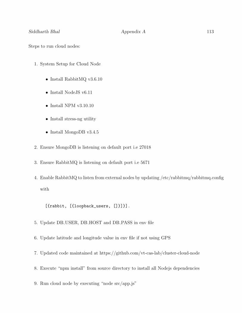
Siddharth Bhal Appendix A 113
Steps to run cloud nodes:
1. System Setup for Cloud Node
• Install RabbitMQ v3.6.10
• Install NodeJS v6.11
• Install NPM v3.10.10
• Install stress-ng utility
• Install MongoDB v3.4.5
2. Ensure MongoDB is listening on default port i.e 27018
3. Ensure RabbitMQ is listening on default port i.e 5671
4. Enable RabbitMQ to listen from external nodes by updating /etc/rabbitmq/rabbitmq.config
with
[{rabbit, [{loopback_users, []}]}].
5. Update DB USER, DB HOST and DB PASS in env file
6. Update latitude and longitude value in env file if not using GPS
7. Updated code maintained at https://github.com/vt-cas-lab/cluster-cloud-node
8. Execute “npm install” from source directory to install all Nodejs dependencies
9. Run cloud node by executing “node src/app.js”
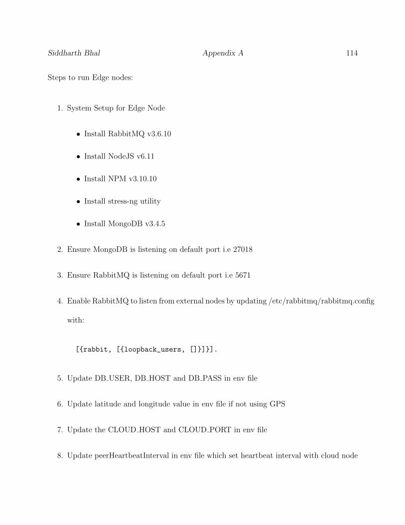
Siddharth Bhal Appendix A 114
Steps to run Edge nodes:
1. System Setup for Edge Node
• Install RabbitMQ v3.6.10
• Install NodeJS v6.11
• Install NPM v3.10.10
• Install stress-ng utility
• Install MongoDB v3.4.5
2. Ensure MongoDB is listening on default port i.e 27018
3. Ensure RabbitMQ is listening on default port i.e 5671
4. Enable RabbitMQ to listen from external nodes by updating /etc/rabbitmq/rabbitmq.config
with:
[{rabbit, [{loopback_users, []}]}].
5. Update DB USER, DB HOST and DB PASS in env file
6. Update latitude and longitude value in env file if not using GPS
7. Update the CLOUD HOST and CLOUD PORT in env file
8. Update peerHeartbeatInterval in env file which set heartbeat interval with cloud node
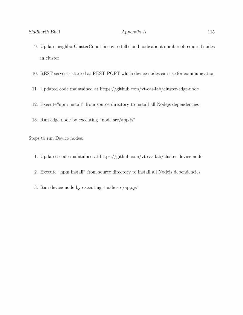
Siddharth Bhal Appendix A 115
9. Update neighborClusterCount in env to tell cloud node about number of required nodes
in cluster
10. REST server is started at REST PORT which device nodes can use for communication
11. Updated code maintained at https://github.com/vt-cas-lab/cluster-edge-node
12. Execute“npm install” from source directory to install all Nodejs dependencies
13. Run edge node by executing “node src/app.js”
Steps to run Device nodes:
1. Updated code maintained at https://github.com/vt-cas-lab/cluster-device-node
2. Execute “npm install” from source directory to install all Nodejs dependencies
3. Run device node by executing “node src/app.js”