fluid flow in porous media
DESCRIPTION
Infinite Acting Radial Flow EquationsTRANSCRIPT
M.Sc. in Petroleum Engineering Flow in Porous Media Section 1 2002-2003 Dr. R. W. Zimmerman Page 1
1. Diffusion Equation for Fluid Flow in Porous Rocks 1.1. Darcy’s law and the definition of permeability The basic law governing the flow of fluids through porous media is Darcy’s law, which was formulated by the French civil engineer Henry Darcy in 1856 on the basis of his experiments on vertical water filtration through sand beds. Darcy found that his data could be described by
Q =
CAΔ(P − ρgz)L
(1)
where: P = pressure [Pa]
ρ = density [kg/m3]
g = gravitational acceleration [m/s2]
z = vertical coordinate (measured downwards) [m]
L = length of sample [m]
Q = volumetric flowrate [m3/s]
C = constant of proportionality [m2/Pa s]
A = cross-sectional area of sample [m2]
Any consistent set of units can be used in Darcy’s law, such as SI units, cgs units, British engineering units, etc. Unfortunately, in the oil industry it is common to use “oilfield units”, which are not consistent. Darcy’s law is mathematically analogous to other linear phenomenological transport laws, such as Ohm’s law for electrical conduction, Fick’s law for solute diffusion, or Fourier’s law for heat conduction.
Department of Earth Science and Engineering Imperial College
M.Sc. in Petroleum Engineering Flow in Porous Media Section 1 2002-2003 Dr. R. W. Zimmerman Page 2
• Why does the term “ P − ρgz ” govern the flowrate?
Recall from fluid mechanics that Bernoulli’s equation (which essentially embodies the principle of “conservation of energy”) contains the terms
Pρ
− gz +v 2
2=
1ρ
P − ρgz +ρv 2
2
⎛
⎝ ⎜ ⎜
⎞
⎠ ⎟ ⎟ , (2)
where P/ρ is related to the enthalpy per unit mass,
gz is the gravitational energy per unit mass,
v2/2 is the kinetic energy per unit mass.
As fluid velocities in a reservoir are usually very small, the third term is negligible, and we see that the combination “ P − ρgz ” represents an energy-type term. It seems reasonable that the fluid would flow from regions of higher to lower energy, and, therefore, the driving force for flow should be the gradient (i.e., rate of spatial change) of P − ρgz . Subsequent to Darcy’s initial discovery, it has been found that, all other factors being equal, Q is inversely proportional to the fluid viscosity, μ [Pa ⋅s]. It is therefore convenient to factor out μ, and put C = k/μ, where k is known as the permeability, with dimensions [m2].
It is also more convenient to work with the volumetric flow per unit area, q = Q/A. Darcy’s law is therefore usually written as
q =
QA
=kμ
Δ(P − ρgz)L
, (3)
where the flux q has dimensions of [m/s]. It is perhaps easier to think of these units as [m3/m2s].
Department of Earth Science and Engineering Imperial College
M.Sc. in Petroleum Engineering Flow in Porous Media Section 1 2002-2003 Dr. R. W. Zimmerman Page 3
For transient processes in which the flux varies from point-to-point, we need a differential form of Darcy’s law. In the vertical direction, this equation would take the form
qv =
QA
=−kμ
d(P − ρgz)dz
. (4)
The minus sign is included because the fluid flows in the direction from higher to lower potential. The differential form of Darcy’s law for one-dimensional, horizontal flow is
qH =
QA
=−kμ
d(P − ρgz)dx
=−kμ
dPdx
. (5)
In most rocks the permeability kH in the horizontal plane is different than the vertical permeability, kV; in most cases, kH > kV. The permeabilities in any two orthogonal directions within the horizontal plane may also differ. However, in this course we will usually assume that kH = kV.
• The permeability is a function of rock type, and also varies with stress, temperature, etc., but does not depend on the fluid; the effect of the fluid on the flowrate is accounted for by the viscosity term in eq. (4) or (5).
• Permeability has units of m2, but in petroleum engineering it is conventional to use “Darcy” units, defined by
1Darcy = 0.987 × 10⁻¹² m2 ≈ 10−12 m2 . (6)
The Darcy unit is defined such that a rock having a permeability of 1 Darcy would transmit 1 cc of water (with viscosity 1 cP) per second, through a region of 1 sq. cm. cross-sectional area, if the pressure drop along the direction of flow were 1 atm per cm.
Department of Earth Science and Engineering Imperial College
M.Sc. in Petroleum Engineering Flow in Porous Media Section 1 2002-2003 Dr. R. W. Zimmerman Page 4
Many soils and sands that civil engineers must deal with have permeabilities on the order of a few Darcies. The original purpose of the “Darcy” definition was therefore to avoid the need for using small prefixes such as 10-12, etc. Fortunately, a Darcy is nearly a round number in SI units, so conversion between the two units is easy.
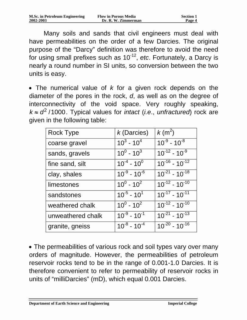
• The numerical value of k for a given rock depends on the diameter of the pores in the rock, d, as well as on the degree of interconnectivity of the void space. Very roughly speaking, k ≈ d2 /1000. Typical values for intact (i.e., unfractured) rock are given in the following table:
Rock Type k (Darcies) k (m2) coarse gravel 103 - 104 10-9 - 10-8
sands, gravels 100 - 103 10-12 - 10-9
fine sand, silt 10-4 - 100 10-16 - 10-12
clay, shales 10-9 - 10-6 10-21 - 10-18
limestones 100 - 102 10-12 - 10-10
sandstones 10-5 - 101 10-17 - 10-11
weathered chalk 100 - 102 10-12 - 10-10
unweathered chalk 10-9 - 10-1 10-21 - 10-13
granite, gneiss 10-8 - 10-4 10-20 - 10-16
• The permeabilities of various rock and soil types vary over many orders of magnitude. However, the permeabilities of petroleum reservoir rocks tend to be in the range of 0.001-1.0 Darcies. It is therefore convenient to refer to permeability of reservoir rocks in units of “milliDarcies” (mD), which equal 0.001 Darcies.
Department of Earth Science and Engineering Imperial College
M.Sc. in Petroleum Engineering Flow in Porous Media Section 1 2002-2003 Dr. R. W. Zimmerman Page 5
• The values in the above table are for intact rock. In some reservoirs, however, the permeability is due mainly to an interconnected network of fractures. The permeabilities of fractured rock masses tend to be in the range 1 mD to 10 Darcies. In a fractured reservoir, the reservoir-scale permeability is not closely related to the core scale permeability that one would measure in the laboratory.
1.2. Datum levels and corrected pressure
If the fluid is in static equilibrium, then q = 0, and eq. (1.1.4) yields
d(P − ρgz)
dz= 0 ⇒ P − ρgz = constant. (1)
If we take z = 0 to be at sea level, where the fluid pressure is atmospheric, then
Pstatic(z) = Patm + ρgz . (2)
As we always measure the pressure as “gauge pressure” (i.e., the pressure above atmospheric), we can essentially neglect Patm in eq. (2). We then see by comparing eq. (2) with eq. (1.1.4) that only the pressure above and beyond the static pressure given by eq. (2) plays a role in “driving” the flow. In a sense, then, the term ρgz is superfluous, because it only contributes to the static pressure, but does not contribute to the driving force for flow.
In order to remove this extraneous term, it is common to define a corrected pressure, Pc , as
Pc = P − ρgz . (3)
Department of Earth Science and Engineering Imperial College
M.Sc. in Petroleum Engineering Flow in Porous Media Section 1 2002-2003 Dr. R. W. Zimmerman Page 6
In terms of the corrected pressure, Darcy’s law (for, say, horizontal flow) can be written as
q =
QA
=−kμ
dPcdx
. (4)
Instead of using sea level (z = 0) as the “datum”, we often use some depth zo such that equal amounts of initial oil-in-place lie above and below zo. In this case,
Pc = P − ρg(z − zo ). (5)
The choice of the datum level is immaterial, in the sense that it only contributes a constant term to the corrected pressure, and so does not contribute to the pressure gradient.
The corrected pressure defined in eq. (5) can be interpreted as the pressure of a hypothetical fluid at depth zo that would be in hydrostatic equilibrium with the fluid that exists at the actual pressure at depth z. 1.3. Representative elementary volume
Darcy’s law is a macroscopic law that is intended to be meaningful over regions that are much larger than the size of a single pore. In other words, when we talk about the permeability at a point “(x,y,z)” in the reservoir, we cannot be referring to the permeability at a mathematically infinitesimal “point”, because a given point may, for example, lie in a sand grain, not in the pore space! The property of permeability is in fact only defined for a porous medium, not for an individual pore. Hence, the permeability is a property that is in some sense “averaged out” over a certain region of space surrounded the mathematical point
Department of Earth Science and Engineering Imperial College
M.Sc. in Petroleum Engineering Flow in Porous Media Section 1 2002-2003 Dr. R. W. Zimmerman Page 7
(x,y,z). This region must be large enough to encompass a statistically significant number of pores. Likewise, the “pressure” that we use in Darcy’s law is actually an average pressure taken over a small region of space.
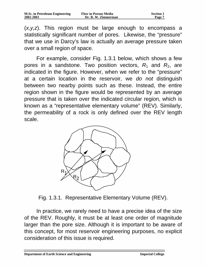
For example, consider Fig. 1.3.1 below, which shows a few pores in a sandstone. Two position vectors, R1 and R2, are indicated in the figure. However, when we refer to the “pressure” at a certain location in the reservoir, we do not distinguish between two nearby points such as these. Instead, the entire region shown in the figure would be represented by an average pressure that is taken over the indicated circular region, which is known as a “representative elementary volume” (REV). Similarly, the permeability of a rock is only defined over the REV length scale.
R1R2
Fig. 1.3.1. Representative Elementary Volume (REV).
In practice, we rarely need to have a precise idea of the size of the REV. Roughly, it must be at least one order of magnitude larger than the pore size. Although it is important to be aware of this concept, for most reservoir engineering purposes, no explicit consideration of this issue is required.
Department of Earth Science and Engineering Imperial College
M.Sc. in Petroleum Engineering Flow in Porous Media Section 1 2002-2003 Dr. R. W. Zimmerman Page 8
1.4. Radial, steady-state flow to a well
Before we proceed to derive the general transient equation that governs flow through porous media, we will examine a simple (but illustrative) problem that can be solved using only Darcy’s law: flow to a well in a circular reservoir that has a constant pressure at its outer boundary.
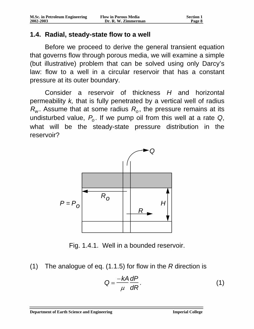
Consider a reservoir of thickness H and horizontal permeability k, that is fully penetrated by a vertical well of radius Rw . Assume that at some radius Ro , the pressure remains at its undisturbed value, Po . If we pump oil from this well at a rate Q, what will be the steady-state pressure distribution in the reservoir?
Q
P = PoRo
RH
Fig. 1.4.1. Well in a bounded reservoir.
(1) The analogue of eq. (1.1.5) for flow in the R direction is
Q =
−kAμ
dPdR
. (1)
Department of Earth Science and Engineering Imperial College
M.Sc. in Petroleum Engineering Flow in Porous Media Section 1 2002-2003 Dr. R. W. Zimmerman Page 9
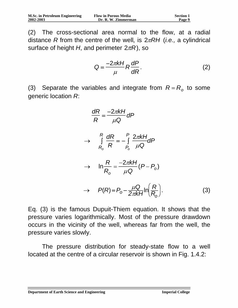
(2) The cross-sectional area normal to the flow, at a radial distance R from the centre of the well, is 2πRH (i.e., a cylindrical surface of height H, and perimeter 2πR), so
Q =
−2πkHμ
R dPdR
. (2)
(3) Separate the variables and integrate from R = Ro to some generic location R:
dRR
=−2πkH
μQdP
→
dRRRo
R∫ = −
2πkHμQPo
P∫ dP
→ ln R
Ro=
−2πkHμQ
(P − Po )
→ P(R) = Po − μQ
2πkH ln RRo
⎛
⎝ ⎜
⎞
⎠ ⎟ . (3)
Eq. (3) is the famous Dupuit-Thiem equation. It shows that the pressure varies logarithmically. Most of the pressure drawdown occurs in the vicinity of the well, whereas far from the well, the pressure varies slowly.
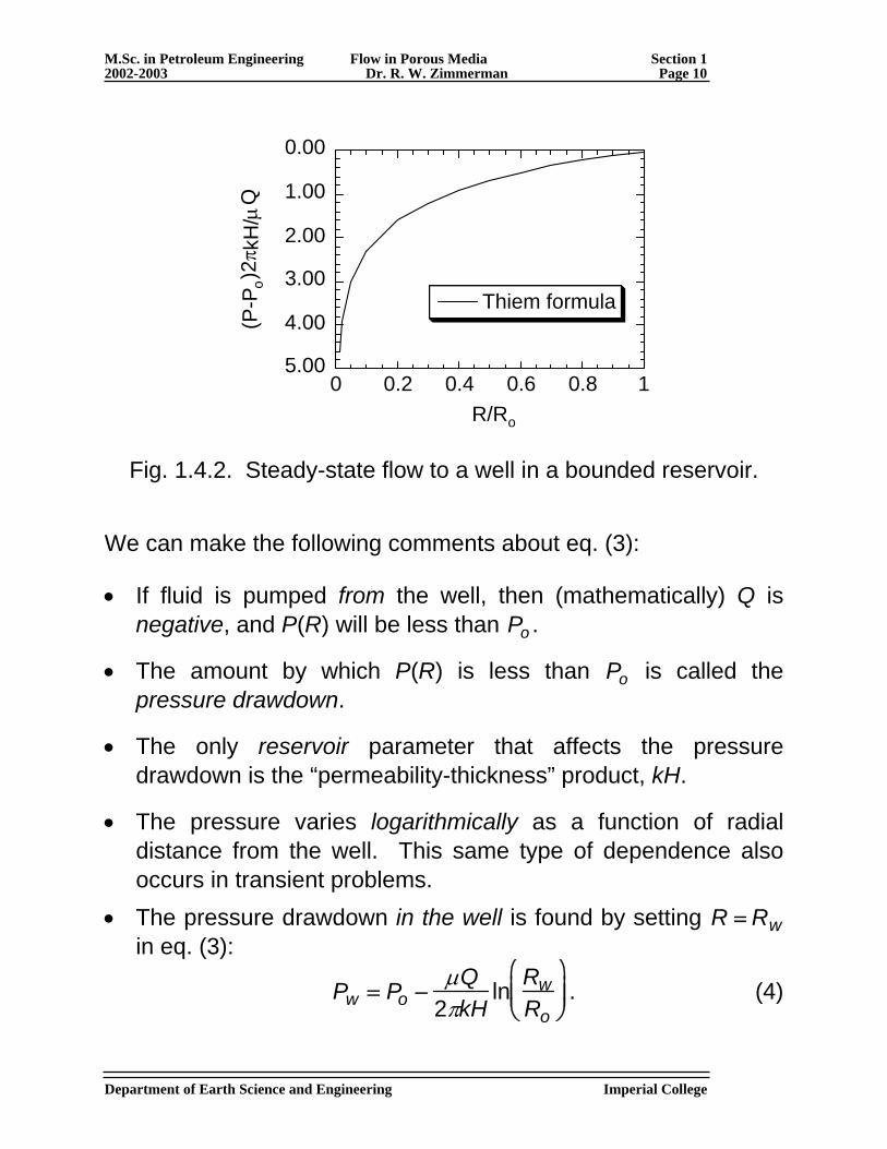
The pressure distribution for steady-state flow to a well located at the centre of a circular reservoir is shown in Fig. 1.4.2:
Department of Earth Science and Engineering Imperial College
M.Sc. in Petroleum Engineering Flow in Porous Media Section 1 2002-2003 Dr. R. W. Zimmerman Page 10
0.00
1.00
2.00
3.00
4.00
5.000 0.2 0.4 0.6 0.8 1
Thiem formula
(P-P
o)2
π kH
/μQ
R/Ro
Fig. 1.4.2. Steady-state flow to a well in a bounded reservoir.
We can make the following comments about eq. (3):
• If fluid is pumped from the well, then (mathematically) Q is negative, and P(R) will be less than Po .
• The amount by which P(R) is less than Po is called the pressure drawdown.
• The only reservoir parameter that affects the pressure drawdown is the “permeability-thickness” product, kH.
• The pressure varies logarithmically as a function of radial distance from the well. This same type of dependence also occurs in transient problems.
• The pressure drawdown in the well is found by setting R = Rw in eq. (3):
Pw = Po −
μQ2πkH
ln RwRo
⎛
⎝ ⎜ ⎜
⎞
⎠ ⎟ ⎟ . (4)
Department of Earth Science and Engineering Imperial College
M.Sc. in Petroleum Engineering Flow in Porous Media Section 1 2002-2003 Dr. R. W. Zimmerman Page 11
• Since we are usually interested in fluid flowing towards the well (i.e., “production”), it is common to define Q > 0 for production, in which case we write eq. (4) as
Pw = Po +
μQ2πkH
ln RwRo
⎛
⎝ ⎜ ⎜
⎞
⎠ ⎟ ⎟ . (5)
1.5. Conservation of mass equation
Darcy’s law in itself does not contain sufficient information to allow us to solve transient (i.e., time-dependent) problems involving subsurface flow. In order to develop a complete governing equation that applies to transient problems, we must first derive a mathematical expression of the principle of conservation of mass.
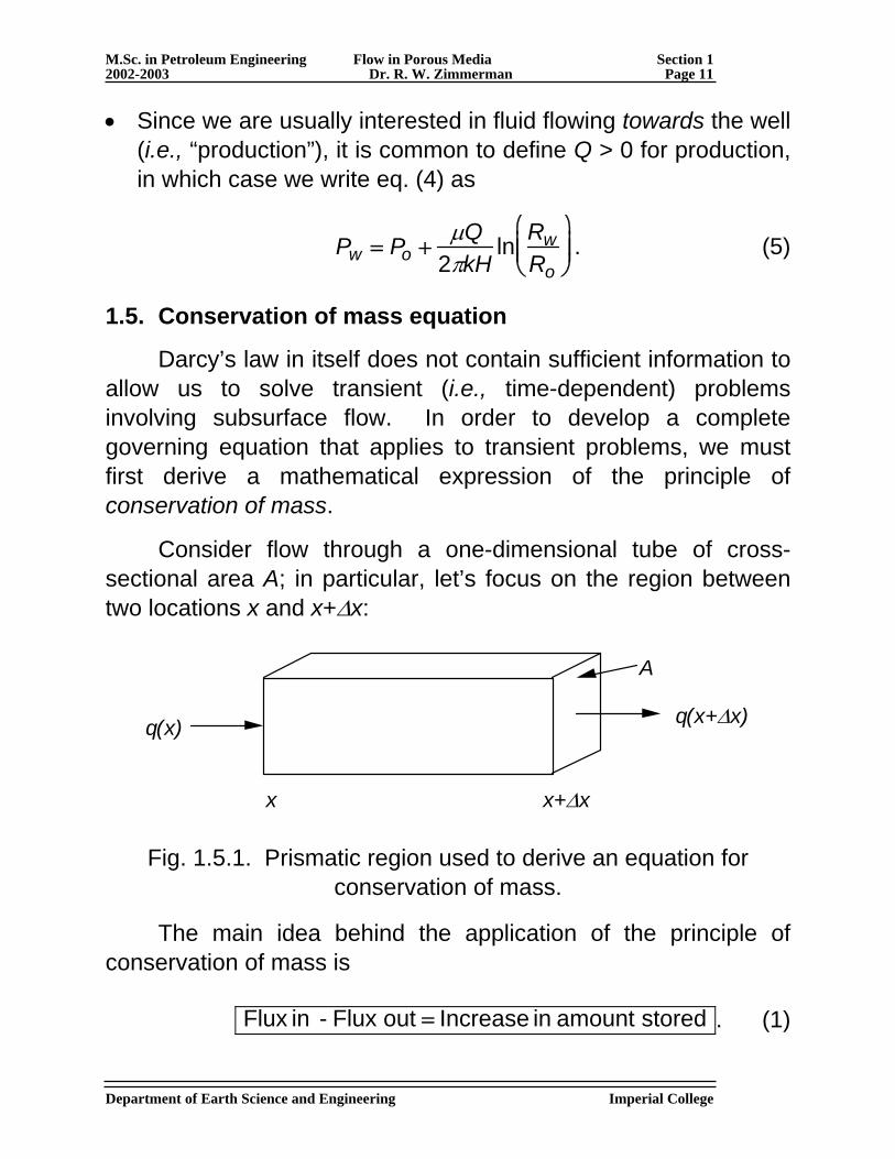
Consider flow through a one-dimensional tube of cross-sectional area A; in particular, let’s focus on the region between two locations x and x+Δx:
q(x) q(x+Δx)
x x+Δx
A
Fig. 1.5.1. Prismatic region used to derive an equation for conservation of mass.
The main idea behind the application of the principle of conservation of mass is
Flux in - Flux out = Increase in amount stored . (1)
Department of Earth Science and Engineering Imperial College
M.Sc. in Petroleum Engineering Flow in Porous Media Section 1 2002-2003 Dr. R. W. Zimmerman Page 12
Note that the property that is conserved is the mass of the fluid, not the volume of the fluid.
Consider the period of time between time t and time t +Δt. To be concrete, assume that the fluid is flowing from left to right through the core. During this time increment, the mass flux into this region of rock between will be
Mass flux in = A(x)ρ(x)q(x)Δt. (2)
The mass flux out of this region of rock will be
Mass flux out = A(x+Δx)ρ(x+Δx)q(x+Δx)Δt. (3)
The amount of fluid mass stored in the region is denoted by m, so the conservation of mass equation takes the form
[A(x)ρ(x)q(x) − A(x + Δx)ρ(x + Δx)q(x + Δx )]Δt
= m(t + Δt) − m(t) . (4)
For one-dimensional flow, such as through a cylindircal core, A(x) = A = constant. So we can factor out A, divide both sides by Δt, and let Δt → 0:
−A[ρq(x + Δx) − ρq(x )] = lim
Δt →0
m(t + Δt) − m(t )Δt
=dmdt
, (5)
where we temporarily treat ρq as a single entity.
But m = ρVp , where V is the pore volume of the rock contained in the slab between x and x+Δx. So,
p
m = ρVp = ρφV = ρφAΔx , (6)
Department of Earth Science and Engineering Imperial College
M.Sc. in Petroleum Engineering Flow in Porous Media Section 1 2002-2003 Dr. R. W. Zimmerman Page 13
→ −A[ρq(x + Δx) − ρq(x )] =
d(ρφ)dt
AΔx . (7)
Now divide both sides by AΔx, and let Δx → 0:
−
d(ρq)dx
=d(ρφ)
dt. (8)
Eq. (8) is the basic equation of conservation of mass for 1-D linear flow in a porous medium. It is exact, and applies to gases, liquids, high or low flowrates, etc.
In its most general, three-dimensional form, the equation of conservation of mass can be written as
d(ρq )dx
+d(ρq )
dy+
d(ρq)dz
= −d(ρφ)
dt. (9)
The mathematical operation on the left-hand side of eq. (9) is known as the divergence of ρq; it represents the rate at which fluid diverges from a given region, per unit volume.
1.6. Diffusion equation in Cartesian coordinates
Transient flow of a fluid through a porous medium is governed by a certain type of partial differential equation known as a diffusion equation. In order to derive this equation, we combine Darcy’s law, the conservation of mass equation, and an equation that describes the manner in which fluid is stored inside a porous rock. (Strangely enough, this last aspect of flow through porous media was only first understood many decades after Darcy’s law was discovered!)
Department of Earth Science and Engineering Imperial College
M.Sc. in Petroleum Engineering Flow in Porous Media Section 1 2002-2003 Dr. R. W. Zimmerman Page 14
Let’s look more closely at the right-hand side of eq. (1.5.8), and use the product rule (and chain rule) of differentiation:
d(ρφ )
dt= ρ dφ
dt+ φ dρ
dt
= ρ dφ
dPdPdt
+ φ dρdP
dPdt
= ρφ 1
φdφdP
⎛
⎝ ⎜ ⎞
⎠ ⎟ + 1
ρdρdP
⎛
⎝ ⎜ ⎞
⎠ ⎟
⎡
⎣ ⎢
⎤
⎦ ⎥ dPdt
= ρφ(cφ +cf )
dPdt , (1)
where cf is the compressibility of the fluid,
cφ is the compressibility of the rock formation.
Now look at the left-hand side of eq. (1.5.8). The flux q is given by Darcy’s law, eq. (1.1.5):
−
d(ρq)dx
= −ddx
−ρkμ
dPdx
⎡
⎣ ⎢ ⎢
⎤
⎦ ⎥ ⎥
=kμ
ρ d 2Pdx 2 +
dρdx
dPdx
⎡
⎣ ⎢ ⎢
⎤
⎦ ⎥ ⎥
=
kμ
ρ d2Pdx 2 +
dρdP
dPdx
dPdx
⎡
⎣ ⎢ ⎢
⎤
⎦ ⎥ ⎥
=
ρkμ
d2Pdx 2 +
1ρ
dρdP
⎛
⎝ ⎜ ⎜
⎞
⎠ ⎟ ⎟
dPdx
⎛
⎝ ⎜ ⎜
⎞
⎠ ⎟ ⎟
2⎡
⎣
⎢ ⎢ ⎢
⎤
⎦
⎥ ⎥ ⎥
Department of Earth Science and Engineering Imperial College
M.Sc. in Petroleum Engineering Flow in Porous Media Section 1 2002-2003 Dr. R. W. Zimmerman Page 15
=
ρkμ
d2Pdx 2 + cf
dPdx
⎛
⎝ ⎜ ⎜
⎞
⎠ ⎟ ⎟
2⎡
⎣
⎢ ⎢ ⎢
⎤
⎦
⎥ ⎥ ⎥ . (2)
Now equate eqs. (1) and (2) to arrive at
d2Pdx2
+ cfdPdx
⎛
⎝ ⎜ ⎜
⎞
⎠ ⎟ ⎟
2
=φμ(cf + cφ )
kdPdt
. (3)
The second term on the left is usually negligible compared to the first. To “prove” that this is the case, we can use eq. (1.4.5), and ignore the difference between x and R, to find
cf
dPdx
⎛
⎝ ⎜ ⎜
⎞
⎠ ⎟ ⎟
2
≈ cfμQ
2πkHR⎛
⎝ ⎜ ⎜
⎞
⎠ ⎟ ⎟
2
, (4)
d2Pdx2 ≈
μQ2πkHR2 , (5)
→ Ratio =
cf μQ2πkH
=cf (Po − Pw)ln(Ro /Rw)
. (6)
Typical values of these parameters (for liquids) are
cf ≈ 10−10 /Pa,
Po − Pw ≈ 10 MPa = 107 Pa,
ln(Ro / Rw ) ≈ ln(1000 m/ 0.1m) = ln(104 ) ≈ 10,
→ Ratio =
10−10 × 107
10= 10−4 << 1 . (7)
Department of Earth Science and Engineering Imperial College
M.Sc. in Petroleum Engineering Flow in Porous Media Section 1 2002-2003 Dr. R. W. Zimmerman Page 16
This example shows that, for liquids, the nonlinear term in eq. (3) is small. In practice, it is usually neglected. For gases, however, it cannot be neglected (see section 9).
The one-dimensional, linearised form of the diffusion equation is therefore
dPdt
=k
φμct
d 2Pdx2 , (8)
in which the total compressibility is given by
ct = cformation + cfluid = cφ + cf . (9)
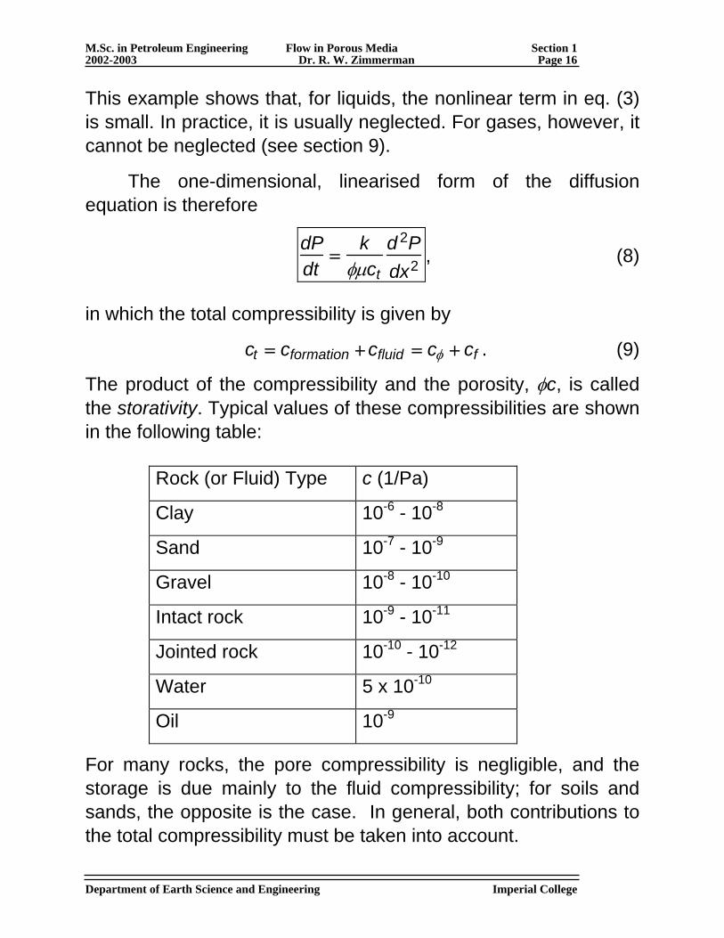
The product of the compressibility and the porosity, φc, is called the storativity. Typical values of these compressibilities are shown in the following table:
Rock (or Fluid) Type c (1/Pa)
Clay 10-6 - 10-8
Sand 10-7 - 10-9
Gravel 10-8 - 10-10
Intact rock 10-9 - 10-11
Jointed rock 10-10 - 10-12
Water 5 x 10⁻¹⁰
Oil 10-9
For many rocks, the pore compressibility is negligible, and the storage is due mainly to the fluid compressibility; for soils and sands, the opposite is the case. In general, both contributions to the total compressibility must be taken into account.
Department of Earth Science and Engineering Imperial College
M.Sc. in Petroleum Engineering Flow in Porous Media Section 1 2002-2003 Dr. R. W. Zimmerman Page 17
Much of the remainder of this module will be devoted to solving the diffusion equation in various situations. For now, we make the following general remarks about it:
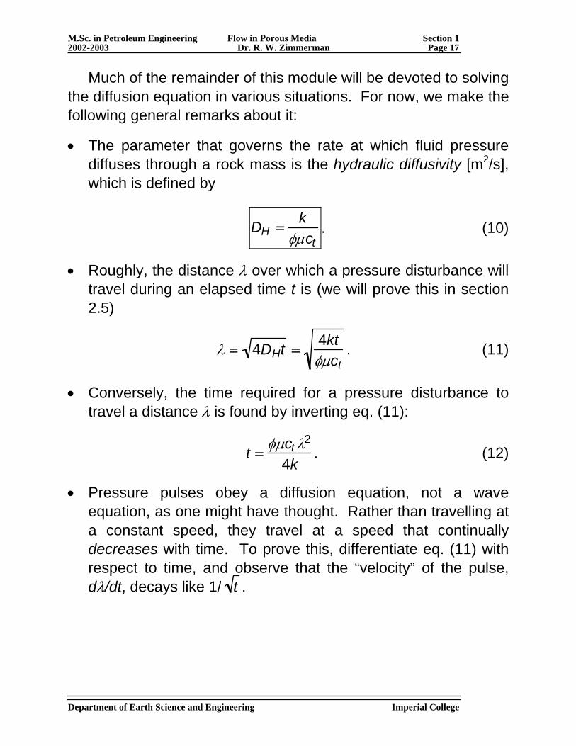
• The parameter that governs the rate at which fluid pressure diffuses through a rock mass is the hydraulic diffusivity [m2/s], which is defined by
DH =
kφμct
. (10)
• Roughly, the distance λ over which a pressure disturbance will travel during an elapsed time t is (we will prove this in section 2.5)
λ = 4DHt =
4ktφμct
. (11)
• Conversely, the time required for a pressure disturbance to travel a distance λ is found by inverting eq. (11):
t =
φμct λ2
4k. (12)
• Pressure pulses obey a diffusion equation, not a wave equation, as one might have thought. Rather than travelling at a constant speed, they travel at a speed that continually decreases with time. To prove this, differentiate eq. (11) with respect to time, and observe that the “velocity” of the pulse, dλ/dt, decays like 1/ t .
Department of Earth Science and Engineering Imperial College
M.Sc. in Petroleum Engineering Flow in Porous Media Section 1 2002-2003 Dr. R. W. Zimmerman Page 18
1.7. Diffusion equation in radial coordinates
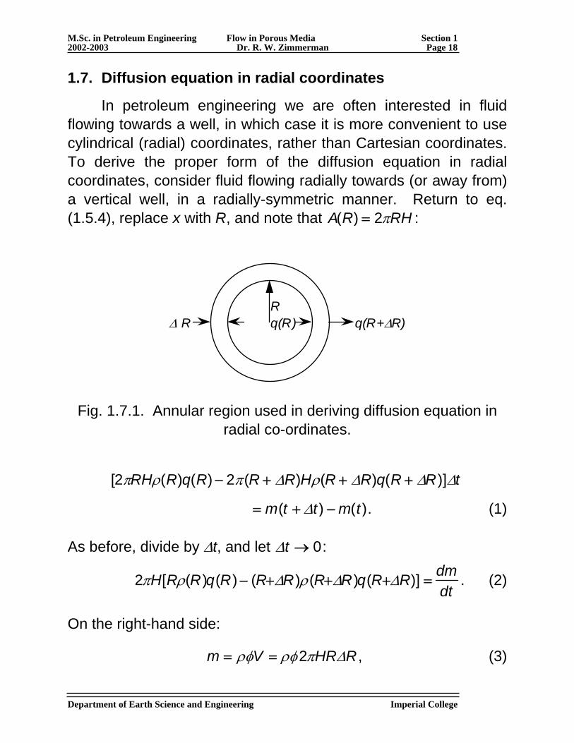
In petroleum engineering we are often interested in fluid flowing towards a well, in which case it is more convenient to use cylindrical (radial) coordinates, rather than Cartesian coordinates. To derive the proper form of the diffusion equation in radial coordinates, consider fluid flowing radially towards (or away from) a vertical well, in a radially-symmetric manner. Return to eq. (1.5.4), replace x with R, and note that A(R) = 2πRH :
RΔ R q(R) q(R+ΔR)
Fig. 1.7.1. Annular region used in deriving diffusion equation in radial co-ordinates.
[2πRHρ(R)q(R) − 2π(R + ΔR)Hρ(R + ΔR)q(R + ΔR)]Δt
= m(t + Δt) − m(t). (1)
As before, divide by Δt, and let Δt → 0:
2πH[Rρ(R)q(R) − (R+ΔR)ρ(R+ΔR)q(R+ΔR)] =
dmdt
. (2)
On the right-hand side:
m = ρφV = ρφ2πHRΔR , (3)
Department of Earth Science and Engineering Imperial College
M.Sc. in Petroleum Engineering Flow in Porous Media Section 1 2002-2003 Dr. R. W. Zimmerman Page 19
→ dmdt
=d(ρφ2πHRΔR)
dt= 2πHR d(ρφ )
dtΔR . (4)
Equate eqs. (2) and (4), divide by ΔR, and let ΔR → 0:
−
d(ρqR)dR
= R d(ρφ )dt
. (5)
Eq. (5) is the radial-flow version of the continuity (i.e., conservation of mass) equation.
Now use Darcy’s law in the form of eq. (1.4.1) for q on the left-hand side, and eq. (1.6.1) on the right-hand side:
kμ
ddR
ρR dPdR
⎛
⎝ ⎜ ⎜
⎞
⎠ ⎟ ⎟ = ρφ(cf + cφ )R dP
dt. (6)
Follow the same procedure as that which led to eq. (1.6.3), to find
1R
ddR
R dPdR
⎛
⎝ ⎜ ⎜
⎞
⎠ ⎟ ⎟ + cf
dPdR
⎛
⎝ ⎜ ⎜
⎞
⎠ ⎟ ⎟
2
=φμ(cf + cφ )
kdPdt
. (7)
For liquids, we again neglect the term cf (dP / dR)2, to arrive at
dPdt
=k
φμct
1R
ddR
R dPdR
⎛
⎝ ⎜ ⎜
⎞
⎠ ⎟ ⎟ . (8)
Eq. (8) is the governing equation for transient, radial flow of a liquid through porous rock. It is the governing equation for flow during primary production, and it is the starting point for all well-test analysis methods. We will develop and analyse solutions to this equation in later parts of this module.
Department of Earth Science and Engineering Imperial College
M.Sc. in Petroleum Engineering Flow in Porous Media Section 1 2002-2003 Dr. R. W. Zimmerman Page 20
1.8. Governing equations for multi-phase flow
In all of the derivations given thus far, we have assumed that the pores of the rock are filled with a single-component, single-phase fluid. Oil reservoirs are typically filled with at least two components, oil and water, and often also contain some hydrocarbons in the gaseous phase. We will now present the governing flow equations for an oil/water system, in a fairly general form.
Recall from the rock properties module that Darcy’s law can be generalised for two-phase flow by including a relative permeability factor for each phase:
qw =
−kkrwμw
dPwdx
, (1)
qo =
−kkroμo
dPodx
, (2)
where the subscripts w and o denote oil and water, respectively. The two relative permeability functions are assumed to be known functions of the phase saturations. For an oil-water system, the two saturations are necessarily related to each other by
Sw + So = 1. (3)
In general, the pressures in the two phases at each “point” in the reservoir will be different. If the reservoir is oil-wet, the two pressures will be related by
Po − Pw = Pcap (So ) , (4)
where the capillary pressure is given by some rock-dependent function of the oil saturation.
Department of Earth Science and Engineering Imperial College
M.Sc. in Petroleum Engineering Flow in Porous Media Section 1 2002-2003 Dr. R. W. Zimmerman Page 21
As the volume of, say, oil, in a given region is equal to the total pore volume multiplied by the oil saturation, the conservation of mass equations for the two phases can be taken directly from eq. (1.5.8), by inserting a saturation factor in the storage term:
−
d(ρoqo )dx
=d(φρoSo)
dt, (5)
−
d(ρwqw )dx
=d(φρwSw)
dt. (6)
The densities of the two phases are related to their respective phase pressures by an equation of state:
ρo = ρo(Po) . (7)
ρw = ρw(Pw) . (8)
where the right-hand sides of eqs. (7) and (8) are known functions of the pressure, and (for our present purposes) the temperature is assumed constant.
Finally, the porosity must be some function of the phase pressures, Po and Pw. Currently, little is known about the manner in which these two pressures independently affect the porosity. Fortunately, the capillary pressure is usually small, and so Po ≈ Pw , in which case we can use the pressure-porosity relationship that would be obtained in a laboratory test performed under single-phase conditions, i.e.,
φ = φ(Po ). (9)
Department of Earth Science and Engineering Imperial College
M.Sc. in Petroleum Engineering Flow in Porous Media Section 1 2002-2003 Dr. R. W. Zimmerman Page 22
Eqs. (1)-(9) give nine equations for the nine unknowns (count them!). In many situations, the equations are simplified to allow solutions to be obtained. For example, in the Buckley-Leverett problem of immiscible displacement (module 4.1), the densities are assumed to be constant, and the capillary pressure is assumed to be zero.
If the fluid is slightly compressible (or if the pressure variations are small), the equations of state are written as
ρ(Po ) = ρoi 1+ co (Po − Poi )[ ], (10)
etc., where the subscript i denotes the initial state, and the compressibility co is taken to be a constant.
______________________________________________ Tutorial Sheet 1:
(1) A well located in a 100 ft. thick reservoir having permeability 100 mD produces 100 barrels/day of oil from a 10 in. diameter wellbore. The viscosity of the oil is 0.4 cP. The pressure at a distance of 1000 feet from the wellbore is 3000 psi. What is the pressure in the wellbore? Conversion factors are as follows: 1 barrel = 0.1589 m3
1 Poise = 0.1 Newton-seconds/m2
1 foot = 0.3048 m 1 psi = 6895 N/ m2 = 6895 Pa
(2) Carry out a derivation of the diffusion equation for spherically-symmetric flow, in analogy to the derivation given in section 1.7 for radial flow. The result should be an equation similar to eq. (1.7.8), but with a slightly different term on the right-hand side.
Department of Earth Science and Engineering Imperial College
M.Sc. in Petroleum Engineering Flow in Porous Media Section 2 2002-2003 Dr. R. W. Zimmerman Page 23
2. Line Source Solution for a Vertical Well in an Infinite Reservoir
One of the most basic and important problems in petroleum reservoir engineering, and the cornerstone of well-test analysis, is the problem of flow of a single-phase, slightly compressible fluid to a vertical well that is located in an infinite reservoir. This problem can be formulated precisely as follows:
• Geometry: a vertical well that fully penetrates a reservoir which is of uniform thickness, H, and which extends infinitely far in all horizontal directions.
• Reservoir Properties: the reservoir is assumed to be isotropic and homogeneous, with constant properties (i.e., permeability, etc.) that do not vary with pressure.
• Initial and Boundary Conditions: the reservoir is initially at uniform pressure. Starting at t = 0, fluid is pumped out of the wellbore at a constant rate, Q.
• Wellbore diameter: it is assumed that the diameter of the wellbore is infinitely small; this leads to a much simpler problem than the more realistic finite-diameter case, but with little loss of applicability, as we will see later.
Problem: to determine the pressure at all points in the reservoir, including in the wellbore, as a function of the elapsed time since the start of production.
The conditions outlined above lead to the so-called line source solution, also known as the Kelvin solution or Theis solution. It was derived by Kelvin in the 1880s in the context of heat conduction; Charles Theis was the first to use it in the context of flow to a well, in 1935. Department of Earth Sciences and Engineering Imperial College
M.Sc. in Petroleum Engineering Flow in Porous Media Section 2 2002-2003 Dr. R. W. Zimmerman Page 24
2.1. Development of the line-source solution
The basic governing equation for this problem is the diffusion equation in radial coordinates, eq. (1.7.8):
φμctk
dPdt
=1R
ddR
R dPdR
⎛
⎝ ⎜ ⎜
⎞
⎠ ⎟ ⎟ . (1)
The assumptions that are inherent in this equation are:
(1) The reservoir is homogeneous and isotropic - i.e., k, φ, etc., do not vary with position in the reservoir, and so they can be assumed to be constant.
(2) The thickness of the reservoir is uniform - this implies that the flow will be horizontal flow to the well, with no vertical component.
(3) The well fully penetrates the entire thickness of the reservoir (or else there would be a vertical flow component).
(4) The fluid is only slightly compressible - this is implicit in treating the compressibility term ct = cf + cφ as a constant.
• If the reservoir is anisotropic, the equations can be modified by a change of variables that is equivalent to stretching the x and y coordinates (de Marsily, pp. 178-9).
• Inhomogeneity is difficult to treat, and methods for this situation are still being developed. Variation in the thickness of the reservoir is somewhat equivalent to spatial variation in k (i.e., inhomogeneity).
• If the well does not fully penetrate the reservoir, we must add d2P/dz2 to the RHS of eq. (1). The solution to this much more difficult problem is discussed by de Marsily, pp. 179-190.
Department of Earth Sciences and Engineering Imperial College
M.Sc. in Petroleum Engineering Flow in Porous Media Section 2 2002-2003 Dr. R. W. Zimmerman Page 25
Department of Earth Sciences and Engineering Imperial College
• The case of a highly compressible fluid, such as a gas, will be discussed in detail in section 9.
To solve the line-source problem, (or to solve any partial differential equation), we not only need a governing equation, but we also need initial conditions and boundary conditions. In this case they are as follows.
Initial Condition: At the start of production, the pressure in the reservoir is assumed to be at some uniform value, Pi .
Boundary condition at infinity: Infinitely far from the well, the pressure will always remain at its initial value, Pi .
Boundary condition at the wellbore: At the wellbore, which is assumed to be infinitely small, the flux must be equal to Q (into the well) at all times t > 0.
We can therefore formulate the problem in precise mathematical terms as follows:
Governing PDE:
1R
ddR
R dPdR
⎡
⎣ ⎢ ⎢
⎤
⎦ ⎥ ⎥
=φμc
kdPdt
, (1)
Initial condition: P(R,t = 0) = Pi , (2)
BC at wellbore: R→0lim
2πkHμ
R dPdR
⎛
⎝ ⎜ ⎜
⎞
⎠ ⎟ ⎟ = Q , (3)
BC at infinity: R→∞lim P(R,t) = Pi . (4)
There are many ways to solve this equation, but we will solve it using a method that avoids advanced techniques such as Laplace transforms, etc.
M.Sc. in Petroleum Engineering Flow in Porous Media Section 2 2002-2003 Dr. R. W. Zimmerman Page 26
First define a new variable using the Boltzmann transformation:
η =
φμcR2
kt. (5)
Now, rewrite eq. (1) in terms of the new variable, η. The right-hand side transforms as follows:
dPdR
=dPdη
dηdR
=2φμcR
ktdPdη
=φμcR2
kt2R
dPdη
=2ηR
dPdη
. (6)
So we see that differentiation with respect to R is equivalent to differentiation with respect to η, followed by multiplication by 2η/R. Hence,
1R
ddR
R dPdR
⎡
⎣ ⎢ ⎢
⎤
⎦ ⎥ ⎥
=1R
2ηR
ddη
2η dPdη
⎛
⎝ ⎜ ⎜
⎞
⎠ ⎟ ⎟ =
4ηR2
ddη
η dPdη
⎛
⎝ ⎜ ⎜
⎞
⎠ ⎟ ⎟ . (7)
The left-hand side of eq. (1) transforms as follows:
dPdt
=dPdη
dηdt
= −φμcR2
kt2dPdη
=−ηt
dPdη
,
→
φμck
dPdt
=−φμc
kηt
dPdη
=−φμcR2
ktηR2
dPdη
=−η2
R2dPdη
. (8)
Using eqs. (7) and (8) in eq. (1) yields
ddη
η dPdη
⎛
⎝ ⎜ ⎜
⎞
⎠ ⎟ ⎟ = −
η4
dPdη
. (9)
Department of Earth Sciences and Engineering Imperial College
M.Sc. in Petroleum Engineering Flow in Porous Media Section 2 2002-2003 Dr. R. W. Zimmerman Page 27
Eq. (9) is an ordinary differential equation for P as a function of η.
We must also transform the boundary/initial conditions so that they apply to P(η) instead of to P(r,t). First note that both limits, R → ∞ and t → 0 , correspond to the limit η → ∞ . Hence, conditions (2,4) take the form
η→∞lim P(η) = Pi . (10)
Using eq. (6) in eq. (3) leads to a second BC:
η→0lim
4πkHμ
ηdPdη
⎛
⎝ ⎜ ⎜
⎞
⎠ ⎟ ⎟ = Q ,
→ η→0lim ηdP
dη
⎛
⎝ ⎜ ⎜
⎞
⎠ ⎟ ⎟ =
μQ4πkH
. (11)
The problem is now a two-point ODE boundary-value problem, defined by eqs. (9-11).
To solve this problem, we first note that although eq. (9) appears to be a 2nd-order equation, it is actually a first-order equation for the function η(dP/dη). If we temporarily denote this combination of terms by y, we can write eq. (9) as
dydη
= −y4
, where y = η dPdη
, (12)
Now separate the variables, and integrate from η = 0 out to an arbitrary value of η:
dyy
= −dη4
Department of Earth Sciences and Engineering Imperial College
M.Sc. in Petroleum Engineering Flow in Porous Media Section 2 2002-2003 Dr. R. W. Zimmerman Page 28
⇒
dyyy (0)
y(η)∫ = −
dη40
η∫
⇒ ln y(η)
y(0)
⎡
⎣ ⎢ ⎢
⎤
⎦ ⎥ ⎥
= −η4
⇒ y(η) = y (0)e −η / 4. (13)
Now note that the boundary condition (11) is equivalent to
y(0) =
μQ4πkH
, (14)
which implies that eq. (13) can be written as
y(η) =
μQ4π kH
e−η / 4. (15)
Recall that y = η(dP / dη), and rewrite eq. (15) as
dP(η)
dη=
μQ4πkH
e −η / 4
η. (16)
Eq. (16) can now be directly integrated to find P(η). We cannot start the integral at η = 0, because we do not know the pressure in the wellbore. We do, however, know from eq. (10) that the pressure at η = ∞ must be equal to the initial pressure, Pi. Therefore,
Department of Earth Sciences and Engineering Imperial College
M.Sc. in Petroleum Engineering Flow in Porous Media Section 2 2002-2003 Dr. R. W. Zimmerman Page 29
dP
Pi
P(η)∫ =
μQ4π kH
e−η / 4
η∞
η∫ dη
⇒ P(η) = Pi −
μQ4πkH
e −η / 4
ηη
∞∫ dη. (17)
Now recall that η = φμcR2 / kt . We replace η with φμcR2 / kt on the left-hand side of eq. (17), and also at the lower limit of integration on the right, but not inside the integral, because inside the integral, η is merely a dummy variable:
P φμcR2
kt
⎛
⎝ ⎜ ⎜
⎞
⎠ ⎟ ⎟ = Pi −
μQ4π kH
e −η / 4
ηφμcR2
kt
∞∫ dη. (18)
Simplify the integrand by defining u = η / 4, in which case dη /η = du / u , and the lower limit of integration becomes u = φμcR2 / 4kt :
P φμcR2
4kt
⎛
⎝ ⎜ ⎜
⎞
⎠ ⎟ ⎟ = Pi −
μQ4π kH
e −u
uφμcR2
4kt
∞∫ du . (19)
The integral in eq. (19) is essentially the so-called “exponential integral function”, which is defined by mathematicians as (see Matthews and Russell, p. 131)
−Ei(−x) =
e−u
ux
∞
∫ du . (20)
Unfortunately, this function was defined long before it was first used to solve the problem of a well in an infinite reservoir, and so it contains extraneous minus signs that are inconvenient.
Department of Earth Sciences and Engineering Imperial College
M.Sc. in Petroleum Engineering Flow in Porous Media Section 2 2002-2003 Dr. R. W. Zimmerman Page 30
We can summarise the solution to this problem as follows:
P(R,t) = Pi +
μQ4πkH
Ei(−x) , (21)
where −Ei(−x) =
e−u
ux
∞
∫ du , (22)
and x = φμcR2 / 4kt . (23)
Numerical values for the pressure drawdown are found as follows. Assume that we want to know the pressure at a certain distance R from the centre of the well, at some time t.
(a) Use these values of R and t to compute a value of x from eq. (23).
(b) Look up the value of -Ei(-x) from a table or graph of the exponential integral function (see next page).
(c) The pressure at (R,t) is then given by eq. (21).
In practice, the more common situation is that the pressure is measured at some distance from the well, as a function of time, and the data is used to infer the values for the reservoir parameters, by fitting the data to the analytical solution. This procedure will be demonstrated after first analysing the line-source solution in more detail.
Note: to find the pressure in the wellbore, we merely plug R = Rw into eq. (21)! This is because R = Rw corresponds to the wellbore wall, where the pressure must be the same as in the wellbore.
Tabular values of the Ei function are shown below. The table is based on the one given by de Marsily, Quantitative Hydrogeology, Academic Press, 1986:
Department of Earth Sciences and Engineering Imperial College
M.Sc. in Petroleum Engineering Flow in Porous Media Section 2 2002-2003 Dr. R. W. Zimmerman Page 31
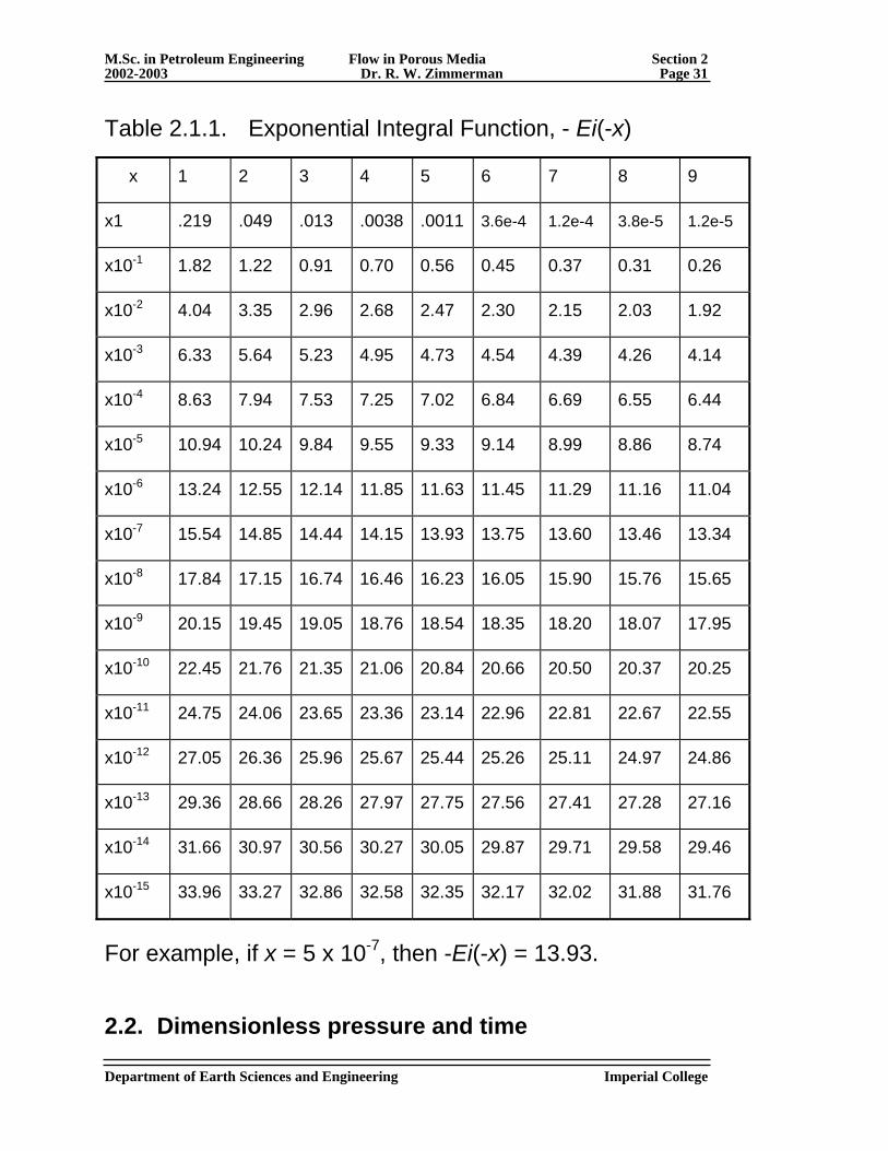
Table 2.1.1. Exponential Integral Function, - Ei(-x)
x 1 2 3 4 5 6 7 8 9
x1 .219 .049 .013 .0038 .0011 3.6e-4 1.2e-4 3.8e-5 1.2e-5
x10-1 1.82 1.22 0.91 0.70 0.56 0.45 0.37 0.31 0.26
x10-2 4.04 3.35 2.96 2.68 2.47 2.30 2.15 2.03 1.92
x10-3 6.33 5.64 5.23 4.95 4.73 4.54 4.39 4.26 4.14
x10-4 8.63 7.94 7.53 7.25 7.02 6.84 6.69 6.55 6.44
x10-5 10.94 10.24 9.84 9.55 9.33 9.14 8.99 8.86 8.74
x10-6 13.24 12.55 12.14 11.85 11.63 11.45 11.29 11.16 11.04
x10-7 15.54 14.85 14.44 14.15 13.93 13.75 13.60 13.46 13.34
x10-8 17.84 17.15 16.74 16.46 16.23 16.05 15.90 15.76 15.65
x10-9 20.15 19.45 19.05 18.76 18.54 18.35 18.20 18.07 17.95
x10-10 22.45 21.76 21.35 21.06 20.84 20.66 20.50 20.37 20.25
x10-11 24.75 24.06 23.65 23.36 23.14 22.96 22.81 22.67 22.55
x10-12 27.05 26.36 25.96 25.67 25.44 25.26 25.11 24.97 24.86
x10-13 29.36 28.66 28.26 27.97 27.75 27.56 27.41 27.28 27.16
x10-14 31.66 30.97 30.56 30.27 30.05 29.87 29.71 29.58 29.46
x10-15 33.96 33.27 32.86 32.58 32.35 32.17 32.02 31.88 31.76
For example, if x = 5 x 10⁻⁷, then -Ei(-x) = 13.93.
2.2. Dimensionless pressure and time Department of Earth Sciences and Engineering Imperial College
M.Sc. in Petroleum Engineering Flow in Porous Media Section 2 2002-2003 Dr. R. W. Zimmerman Page 32
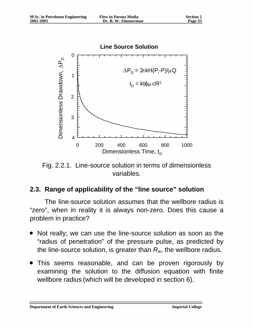
Although the pressure drawdown seems to depend on many variables and parameters, there are only two independent, dimensionless mathematical variables in the line-source solution. This can be proven from the pi-theorem of dimensional analysis, or can be seen directly from eqs. (2.1.21-23). Traditionally, these variables are defined as the dimensionless time,
tD =
ktφμcR2
, (1)
and the dimensionless pressure drawdown,
ΔPD =
2πkH(Pi − P)μQ
. (2)
In terms of these dimensionless parameters, the line-source solution takes the form
ΔPD = −
12
Ei(−1/ 4tD ). (3)
The usefulness of dimensionless variables is that they allow the pressure drawdown to be plotted and discussed in a form that is applicable to all reservoirs, without being restricted to specific values of the permeability, porosity, etc. These parameters are accounted for by the definitions of the dimensionless variables.
Department of Earth Sciences and Engineering Imperial College
M.Sc. in Petroleum Engineering Flow in Porous Media Section 2 2002-2003 Dr. R. W. Zimmerman Page 33
4
-7
3
-5
-4
-3
-2
-1
0
0 200 400 600 800 1000
Line Source Solution
Dim
ensi
onle
ss D
raw
dow
n, Δ
PD
Dimensionless Time, tD
ΔPD = 2πkH(Pi-P)/μQ
tD = kt/φμcR2
0
2
1
3
4
Fig. 2.2.1. Line-source solution in terms of dimensionless
variables.
2.3. Range of applicability of the “line source” solution
The line-source solution assumes that the wellbore radius is “zero”, when in reality it is always non-zero. Does this cause a problem in practice?
• Not really; we can use the line-source solution as soon as the “radius of penetration” of the pressure pulse, as predicted by the line-source solution, is greater than Rw, the wellbore radius.
• This seems reasonable, and can be proven rigorously by examining the solution to the diffusion equation with finite wellbore radius (which will be developed in section 6).
Department of Earth Sciences and Engineering Imperial College
M.Sc. in Petroleum Engineering Flow in Porous Media Section 2 2002-2003 Dr. R. W. Zimmerman Page 34
According to eq. (1.6.12), the time required for the pressure pulse to travel at least a distance Rw (starting from the “infinitely-small” hypothetical borehole at R = 0) is
t >
φμcRw2
4k. (1)
If we use “typical” values for the parameters, such as
φ = 0.20 (a typical reservoir value),
μ = 0.001 Pa s (reasonable for liquid hydrocarbons),
c = 10−10Pa-1 (reasonable for liquid hydrocarbons),
Rw = 0.1m,
k = 10−14m2 (10 mD - somewhat low, but possible),
then eq. (1) predicts that the line-source approximation will become valid after an elapsed time of only 0.005 s!
Note: In terms of the dimensionless time defined by eq. (2.2.1), condition (1) is equivalent to tDw > 0.25, where the subscript w denotes the fact that this is the dimensionless time relative to the position R = R w.
Although one should always check the validity of the line-source approximation, using eq. (1), in practice it is almost always valid.
2.4. Logarithmic approximation to line-source solution
The exponential integral function is unfamiliar to most engineers, and is difficult to calculate. Fortunately, for sufficiently small values of x, which is to say, large values of t, the
Department of Earth Sciences and Engineering Imperial College
M.Sc. in Petroleum Engineering Flow in Porous Media Section 2 2002-2003 Dr. R. W. Zimmerman Page 35
exponential integral essentially becomes a logarithmic function, which makes it very easy to use. To derive this “long-time” approximation, we proceed as follows:
a. For large times, x will be small, and we can break up the integral into two parts:
−Ei(−x) =
e−u
ux
∞
∫ du =e−u
ux
1
∫ du +e −u
u1
∞
∫ du . (1)
b. Use the Taylor series for exp(-u) in the first integrand:
e−u
ux
1∫ du =
1− u1!
+ u2
2!− u3
3!+L
ux
1∫ du . (2)
c. Break up integral into a series of integrals, and evaluate them term-by-term:
e−u
ux
1∫ du =
1ux
1∫ du −
11!
dux
1∫ +
12!
udux
1∫ +
13!
u2du −Lx
1∫
= lnu]x
1− u]x
1+
12!
u2
2
⎤
⎦ ⎥ ⎥
x
1
−13!
u3
3
⎤
⎦ ⎥ ⎥
x
1
+L
= (ln1− lnx) − (1− x ) +
12!2
(1− x 2) −1
3!3(1− x3 ) +L
= − ln x + x −
12!2
x 2 +1
3!3x3 +L− 1−
12!2
+1
3!3+L
⎧ ⎨ ⎩ ⎪
⎫ ⎬ ⎭ ⎪
Department of Earth Sciences and Engineering Imperial College
→ −Ei(−x) = − ln x − lnγ + x −
12!2
x2 +1
3!3x3 +L, (3)
M.Sc. in Petroleum Engineering Flow in Porous Media Section 2 2002-2003 Dr. R. W. Zimmerman Page 36
where lnγ = 1−
12!2
+1
3!3+L
⎧ ⎨ ⎩ ⎪
⎫ ⎬ ⎭ ⎪ −
e −u
u1
∞∫ du . (4)
Eq. (4) may look messy, but the important point is that the term lnγ is merely a number, and does not depend on x, so we can evaluate it numerically to find
lnγ = ln(1.781) = 0.5772. (5)
[Note: Both γ and lnγ are sometimes known as “Euler’s number”, so be careful when reading the literature on this topic!]
We can further simplify eq. (3) if we can find conditions under which the power series terms are negligible. If this is the case, we are left with only a log term and a constant.
First, recall that large t implies small x, and so
x −
12!2
x 2 +1
3!3x 3 +L < x . (6)
If we want the power series terms to be, say, two orders of magnitude less than γ (which itself is ~1), then we need
x =
φμcR2
4kt< 0.01 ⇒
ktφμcR2 > 25. (7)
So, if the dimensionless time is greater than about 25, we have from eqs. (2.1.21) and (3):
P(R,t) = Pi +
μQ4πkH
ln x + lnγ[ ]
Department of Earth Sciences and Engineering Imperial College
M.Sc. in Petroleum Engineering Flow in Porous Media Section 2 2002-2003 Dr. R. W. Zimmerman Page 37
⇒ P(R,t ) = Pi +
μQ4π kH
ln(xγ )
⇒ P(R,t ) = Pi +
μQ4π kH
ln φμcR2γ4kt
⎛
⎝ ⎜ ⎜
⎞
⎠ ⎟ ⎟
⇒ P(R,t ) = Pi −
μQ4π kH
ln 4ktφμcR2γ
⎛
⎝ ⎜ ⎜
⎞
⎠ ⎟ ⎟
⇒ P(R,t) = Pi − μQ
4π kH ln 2.246ktφμcR2
⎛
⎝ ⎜
⎞
⎠ ⎟ (8)
⇒ P(R,t ) = Pi −
μQ4π kH
ln ktφμcR2
⎛
⎝ ⎜ ⎜
⎞
⎠ ⎟ ⎟ + 0.80907
⎡
⎣ ⎢ ⎢
⎤
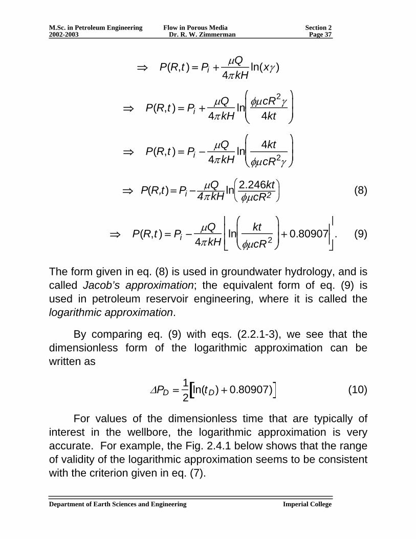
⎦ ⎥ ⎥ . (9)
The form given in eq. (8) is used in groundwater hydrology, and is called Jacob’s approximation; the equivalent form of eq. (9) is used in petroleum reservoir engineering, where it is called the logarithmic approximation.
By comparing eq. (9) with eqs. (2.2.1-3), we see that the dimensionless form of the logarithmic approximation can be written as
ΔPD =
12
ln(tD) + 0.80907)[ ] (10)
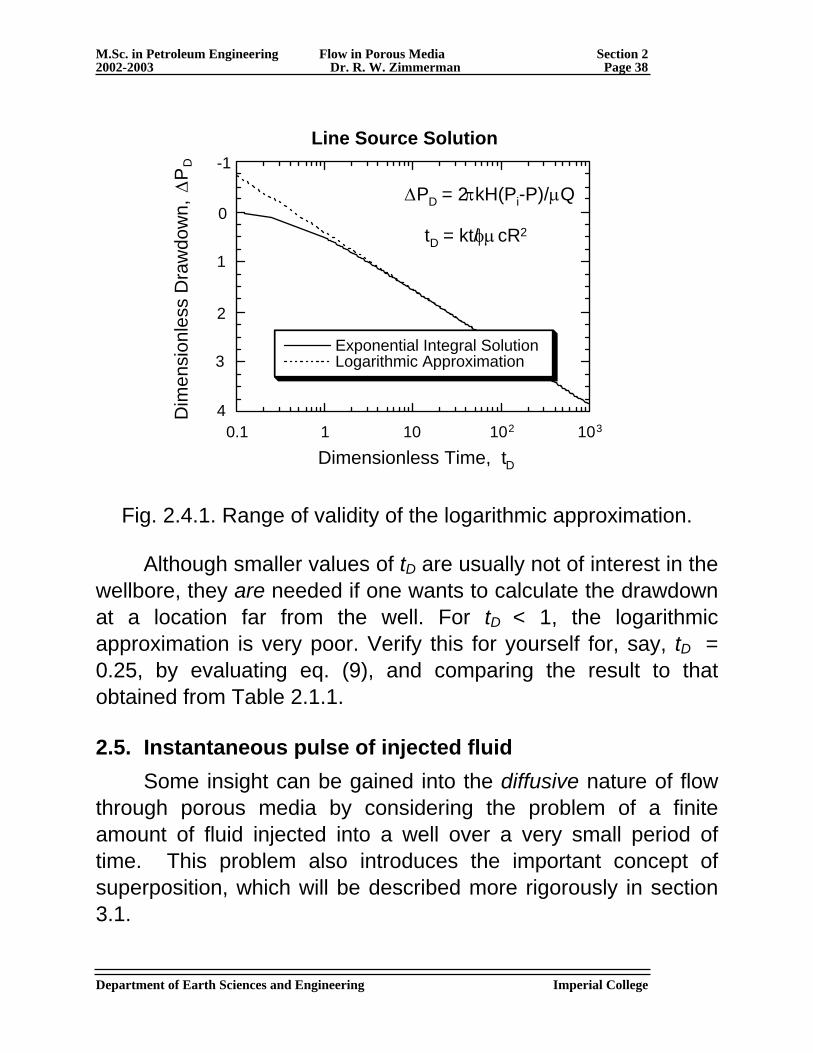
For values of the dimensionless time that are typically of interest in the wellbore, the logarithmic approximation is very accurate. For example, the Fig. 2.4.1 below shows that the range of validity of the logarithmic approximation seems to be consistent with the criterion given in eq. (7).
Department of Earth Sciences and Engineering Imperial College
M.Sc. in Petroleum Engineering Flow in Porous Media Section 2 2002-2003 Dr. R. W. Zimmerman Page 38
0.1 1 10 102 103
Line Source Solution
Exponential Integral SolutionLogarithmic Approximation
Dim
ensi
onle
ss D
raw
dow
n, Δ
PD
Dimensionless Time, tD
tD = kt/φμcR2
ΔPD = 2πkH(Pi-P)/μQ
-1
0
1
3
4
2
Fig. 2.4.1. Range of validity of the logarithmic approximation.
Although smaller values of tD are usually not of interest in the wellbore, they are needed if one wants to calculate the drawdown at a location far from the well. For tD < 1, the logarithmic approximation is very poor. Verify this for yourself for, say, tD = 0.25, by evaluating eq. (9), and comparing the result to that obtained from Table 2.1.1.
2.5. Instantaneous pulse of injected fluid Some insight can be gained into the diffusive nature of flow through porous media by considering the problem of a finite amount of fluid injected into a well over a very small period of time. This problem also introduces the important concept of superposition, which will be described more rigorously in section 3.1.
Department of Earth Sciences and Engineering Imperial College
M.Sc. in Petroleum Engineering Flow in Porous Media Section 2 2002-2003 Dr. R. W. Zimmerman Page 39
Note: The problem of “injecting” fluid is mathematically equivalent to that of “producing” fluid, except for the sign, but it is easier to visualise the pressure pulse propagating into the reservoir in the case of injection. If we start injecting fluid at a rate Q (m3/s) at time t = 0, then, according to eq. (2.1.21), the pressure at a distance R into the reservoir will be
P(R,t) = Pi +
μQ4πkH
e−u
ux
∞
∫ du, x = φμcR2 / 4kt , (1)
where t is the elapsed time since the start of injection. The + sign is used because we are injecting rather than extracting fluid, so the pressure in the reservoir will increase.
Now imagine that we stop injecting fluid after a small amount of time δt. This is equivalent to injecting fluid at a rate Q starting at t = 0, and then producing fluid at a rate Q (or, equivalently, injecting at a rate -Q) starting at time δt. The pressure drawdown in the reservoir due to this fictitious production would be given by the same line-source solution, except that:
(1) For extraction of fluid we must use a - sign in front of the integral;
(2) If t is the elapsed time since the start of injection, then t-δt will be the elapsed time since the start of the fictitious extraction of fluid (i.e., since the end of injection!)
Hence, the full expression for the pressure will be
Department of Earth Sciences and Engineering Imperial College
P(R,t) = Pi +μQ
4πkHe−u
ux=
φμcR2
4kt
∞
∫ du −μQ
4πkHe−u
ux=
φμcR2
4k(t −δt)
∞
∫ du
M.Sc. in Petroleum Engineering Flow in Porous Media Section 2 2002-2003 Dr. R. W. Zimmerman Page 40
= Pi +μQ
4πkHe−u
ux=
φμcR2
4kt
x= φμcR2
4k(t −δt)
∫ du . (2)
But if δt is small, then the two limits of integration are close together, and we can use the following approximation:
f (x )dx
x1
x2
∫ ≈ f (x1)[x2 − x1] , (3)
which in the present case gives
P(R,t) ≈ Pi +
μQ4πkH
⋅4kt
φμcR2 ⋅e−φμcR2
4kt ⋅φμcR2
4k(t − δt)−
φμcR2
4kt
⎡
⎣ ⎢ ⎢
⎤
⎦ ⎥ ⎥
≈ Pi +
μQ4πkH
⋅4kt
φμcR2 ⋅e−φμcR2
4kt ⋅φμcR2δt
4kt 2
⎡
⎣ ⎢ ⎢
⎤
⎦ ⎥ ⎥
≈ Pi +
μQδt4πkHt
e−φμcR2
4kt . (4)
As Q is the rate of injection in [m3/s], and δt is the duration of the injection, the total volume of injected fluid is Qδt, which we can denote as Q*, with units of [m3].
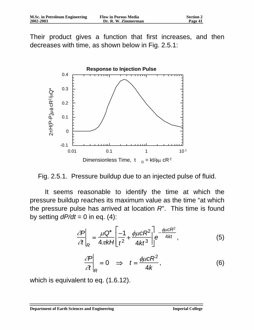
Now imagine that we are monitoring the pressure at some distance R from the borehole. From eq. (4), we se that the pressure buildup at R will be the product of two terms: (a) an exponential term that increases with t, then levels off to a value of 1 as t → ∞ ;
(b) a 1/t term that decays to zero as t → ∞ . Department of Earth Sciences and Engineering Imperial College
M.Sc. in Petroleum Engineering Flow in Porous Media Section 2 2002-2003 Dr. R. W. Zimmerman Page 41
Their product gives a function that first increases, and then decreases with time, as shown below in Fig. 2.5.1:
-0.1
0
0.1
0.2
0.3
0.4
0.01 0.1 1 10 1
Response to Injection Pulse
2πH
(P-P
i)μφ
cR2/μ
Q*
Dimensionless Time, t D = kt/φμ cR 2
Fig. 2.5.1. Pressure buildup due to an injected pulse of fluid.
It seems reasonable to identify the time at which the pressure buildup reaches its maximum value as the time “at which the pressure pulse has arrived at location R”. This time is found by setting dP/dt = 0 in eq. (4):
∂P∂t R
=μQ∗
4πkH−1t 2 +
φμcR2
4kt 3
⎡
⎣ ⎢ ⎢
⎤
⎦ ⎥ ⎥ e
−φμcR2
4kt , (5)
∂P∂t R
= 0 ⇒ t =φμcR2
4k, (6)
which is equivalent to eq. (1.6.12).
Department of Earth Sciences and Engineering Imperial College
M.Sc. in Petroleum Engineering Flow in Porous Media Section 2 2002-2003 Dr. R. W. Zimmerman Page 42
2.6. Estimating permeability and storativity from a drawdown test
In sections 2.1-4 we derived the line-source solution, and showed how to use it to calculate the pressure drawdown, based on assumed knowledge of the reservoir properties. However, the most common use of this solution, and the other solutions that we will derive shortly, is for the inverse problem:
• We use measured wellbore pressures, in conjunction with the mathematical solutions, to estimate reservoir properties such as permeability, porosity, etc.
• This process, known as well-test analysis, is the subject of a subsequent module of the course. For now, we will do one simple example to see how to calculate the reservoir permeability from a drawdown test.
Recall from eq. (2.4.8) that, in the long-time regime,
P(R,t) = Pi −
μQ4πkH
ln 2.246ktφμcR2
⎛
⎝ ⎜ ⎜
⎞
⎠ ⎟ ⎟ . (1)
At the wellbore wall,
P(Rw ,t) = Pi −
μQ4πkH
lnt + ln 2.246kφμcRw
2
⎛
⎝ ⎜ ⎜
⎞
⎠ ⎟ ⎟
⎡
⎣ ⎢ ⎢
⎤
⎦ ⎥ ⎥ . (2)
In general, we will not know the values of any of the parameters on the RHS of eq. (2); we will only know Q, and the wellbore pressure as a function of time, P(Rw ,t ) ≡ Pw(t ). In particular, we don’t know k or φμc, so we can’t use criterion (2.4.7) to find out when our data falls in the late-time regime.
Department of Earth Sciences and Engineering Imperial College
M.Sc. in Petroleum Engineering Flow in Porous Media Section 2 2002-2003 Dr. R. W. Zimmerman Page 43
However, the second logarithmic term, although unknown, is a constant. Hence, if we plot Pw(t ) vs. lnt, the data will (eventually, at large enough values of t) fall on a straight line!
The slope of this line on a semi-log plot gives kH, i.e.,
dPwd lnt
=ΔPwΔ ln t
≡ m =μQ
4π kH, (3)
→ kH =
μQ4πm . (4)
• Q is known, and μ can be measured, so the semi-log slope gives the permeability-thickness product, kH.
• This method is unable to distinguish separately between the effects of permeability and thickness; i.e., a thick impermeable reservoir can give the same drawdown as a thin, permeable reservoir.
Now, let’s do a simple example to learn how to calculate the permeability of a reservoir from a drawdown test.
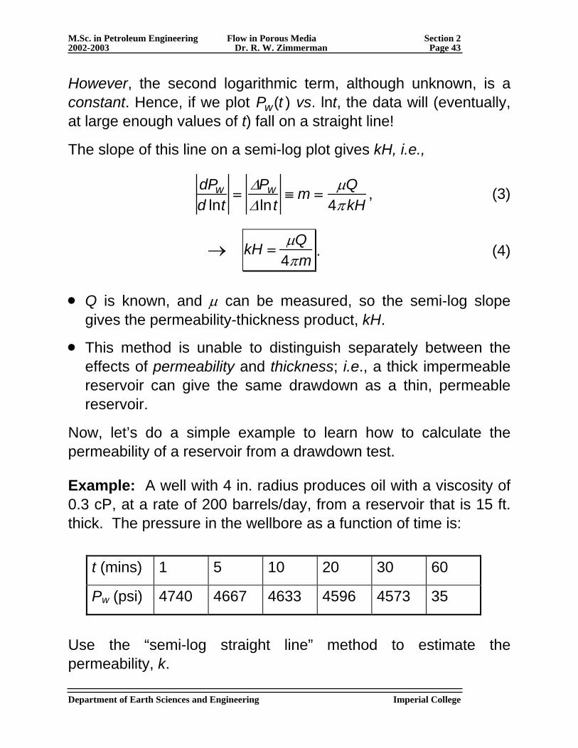
Example: A well with 4 in. radius produces oil with a viscosity of 0.3 cP, at a rate of 200 barrels/day, from a reservoir that is 15 ft. thick. The pressure in the wellbore as a function of time is:
t (mins) 1 5 10 20 30 60
Pw (psi) 4740 4667 4633 4596 4573 35
Use the “semi-log straight line” method to estimate the permeability, k. Department of Earth Sciences and Engineering Imperial College
M.Sc. in Petroleum Engineering Flow in Porous Media Section 2 2002-2003 Dr. R. W. Zimmerman Page 44
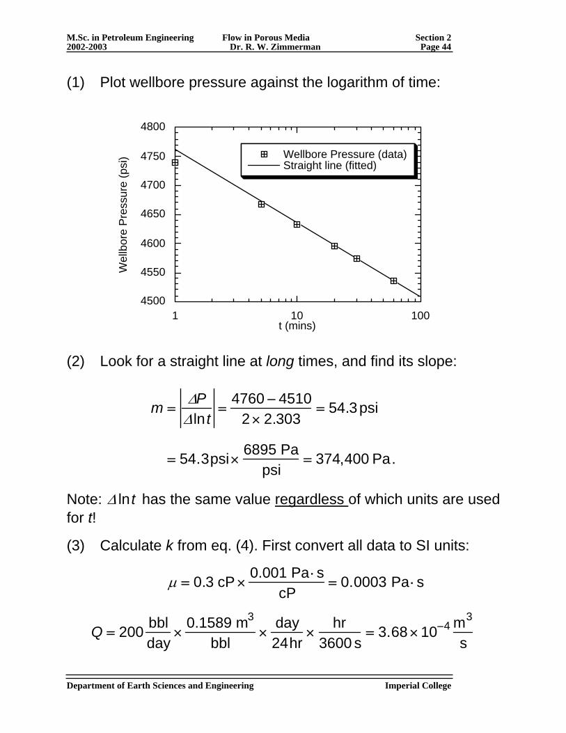
(1) Plot wellbore pressure against the logarithm of time:
4500
4550
4600
4650
4700
4750
4800
1 10 100
Wellbore Pressure (data)Straight line (fitted)
Wel
lbor
e P
ress
ure
(psi
)
t (mins)
(2) Look for a straight line at long times, and find its slope:
m =
ΔPΔ ln t
=4760 − 4510
2 × 2.303= 54.3psi
= 54.3psi ×
6895 Papsi
= 374,400 Pa.
Note: Δ ln t has the same value regardless of which units are used for t!
(3) Calculate k from eq. (4). First convert all data to SI units:
μ = 0.3 cP ×
0.001 Pa ⋅scP
= 0.0003 Pa ⋅s
Q = 200 bbl
day×
0.1589 m3
bbl×
day24hr
×hr
3600 s= 3.68 × 10⁻⁴ m3
s
Department of Earth Sciences and Engineering Imperial College
M.Sc. in Petroleum Engineering Flow in Porous Media Section 2 2002-2003 Dr. R. W. Zimmerman Page 45
H = 15 ft ×
0.3048 mft
= 4.572 m
→ k =
μQ4πmH
=(0.0003Pa s)(3.68 × 10⁻⁴m3/s)
4π(4.572m)(374,400Pa)
= 5.13 × 10⁻¹⁵ m2 ×
1mD0.987 × 10-15 m2 = 5.1mD.
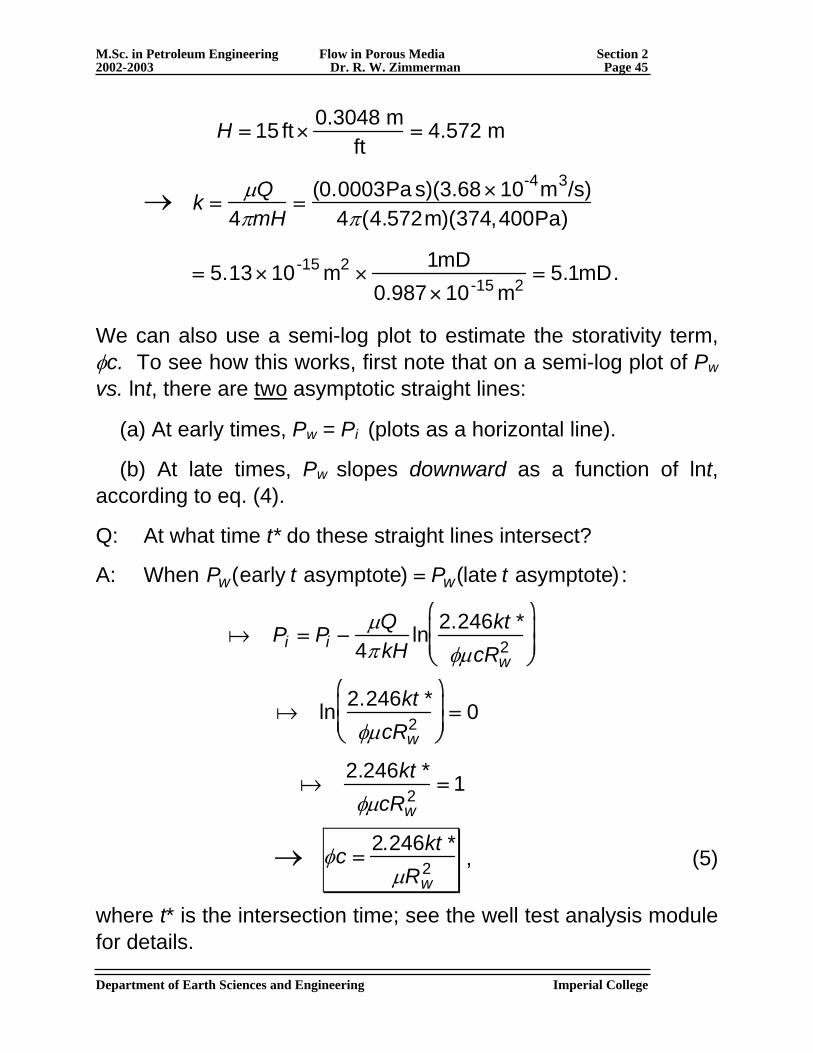
We can also use a semi-log plot to estimate the storativity term, φc. To see how this works, first note that on a semi-log plot of Pw vs. lnt, there are two asymptotic straight lines:
(a) At early times, Pw = Pi (plots as a horizontal line).
(b) At late times, Pw slopes downward as a function of lnt, according to eq. (4).
Q: At what time t* do these straight lines intersect?
A: When Pw(early t asymptote) = Pw(late t asymptote) :
a Pi = Pi −
μQ4π kH
ln 2.246kt *φμcRw
2
⎛
⎝ ⎜ ⎜
⎞
⎠ ⎟ ⎟
a ln 2.246kt *
φμcRw2
⎛
⎝ ⎜ ⎜
⎞
⎠ ⎟ ⎟ = 0
a
2.246kt *φμcRw
2= 1
→ φc =
2.246kt *μRw
2 , (5)
where t* is the intersection time; see the well test analysis module for details. Department of Earth Sciences and Engineering Imperial College
M.Sc. in Petroleum Engineering Flow in Porous Media Section 2 2002-2003 Dr. R. W. Zimmerman Page 46
Department of Earth Sciences and Engineering Imperial College
______________________________________________ Tutorial Sheet 2:
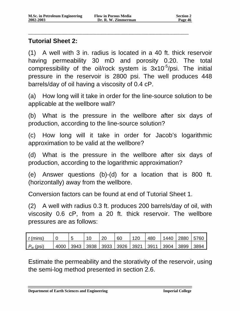
(1) A well with 3 in. radius is located in a 40 ft. thick reservoir having permeability 30 mD and porosity 0.20. The total compressibility of the oil/rock system is 3x10⁻⁵/psi. The initial pressure in the reservoir is 2800 psi. The well produces 448 barrels/day of oil having a viscosity of 0.4 cP.
(a) How long will it take in order for the line-source solution to be applicable at the wellbore wall?
(b) What is the pressure in the wellbore after six days of production, according to the line-source solution?
(c) How long will it take in order for Jacob’s logarithmic approximation to be valid at the wellbore?
(d) What is the pressure in the wellbore after six days of production, according to the logarithmic approximation?
(e) Answer questions (b)-(d) for a location that is 800 ft. (horizontally) away from the wellbore.
Conversion factors can be found at end of Tutorial Sheet 1.
(2) A well with radius 0.3 ft. produces 200 barrels/day of oil, with viscosity 0.6 cP, from a 20 ft. thick reservoir. The wellbore pressures are as follows: t (mins) 0 5 10 20 60 120 480 1440 2880 5760
Pw (psi) 4000 3943 3938 3933 3926 3921 3911 3904 3899 3894
Estimate the permeability and the storativity of the reservoir, using the semi-log method presented in section 2.6.

M.Sc. in Petroleum Engineering Flow in Porous Media Section 3 2003-2004 Dr. R. W. Zimmerman Page 47
3. Superposition and Buildup Tests
3.1. Linearity and the principle of superposition A basic property of the diffusion equation that governs flow of a single-phase compressible liquid through a porous medium is its linearity. Linearity is the most important property that any differential equation can have, because it implies that the principle of superposition can be used to construct solutions to the equation. Most of the analytical methods that have been developed to solve differential equations, such as Laplace transforms, Green’s functions, separation of variables, etc., can be used only on linear differential equations. These analytical methods will be discussed in later sections of this module. In this section we will discuss a simple form of the principle of superposition that will allow us to solve many important reservoir engineering problems, such as pressure buildup tests. The diffusion equation is a linear PDE because both of the differential operators that appear in it are linear operators. In general, a differential operator M that operates on a function F is linear if it has the following two properties:
M(F1+ F2) = M(F1) +M(F2), (1)
M(cF1) = cM(F1), (2)
where F1 and F2 are any two differentiable functions, and c is any constant. The process of partial differentiation is a linear operation, since
ddt
P1(R,t) + P2(R,t)[ ]=dP1(R,t )
dt+
dP2(R,t )dt
, (3)
Department of Earth Science and Engineering Imperial College London
M.Sc. in Petroleum Engineering Flow in Porous Media Section 3 2003-2004 Dr. R. W. Zimmerman Page 48
ddt
cP1(R,t)[ ]= c dP1(R,t)dt
. (4)
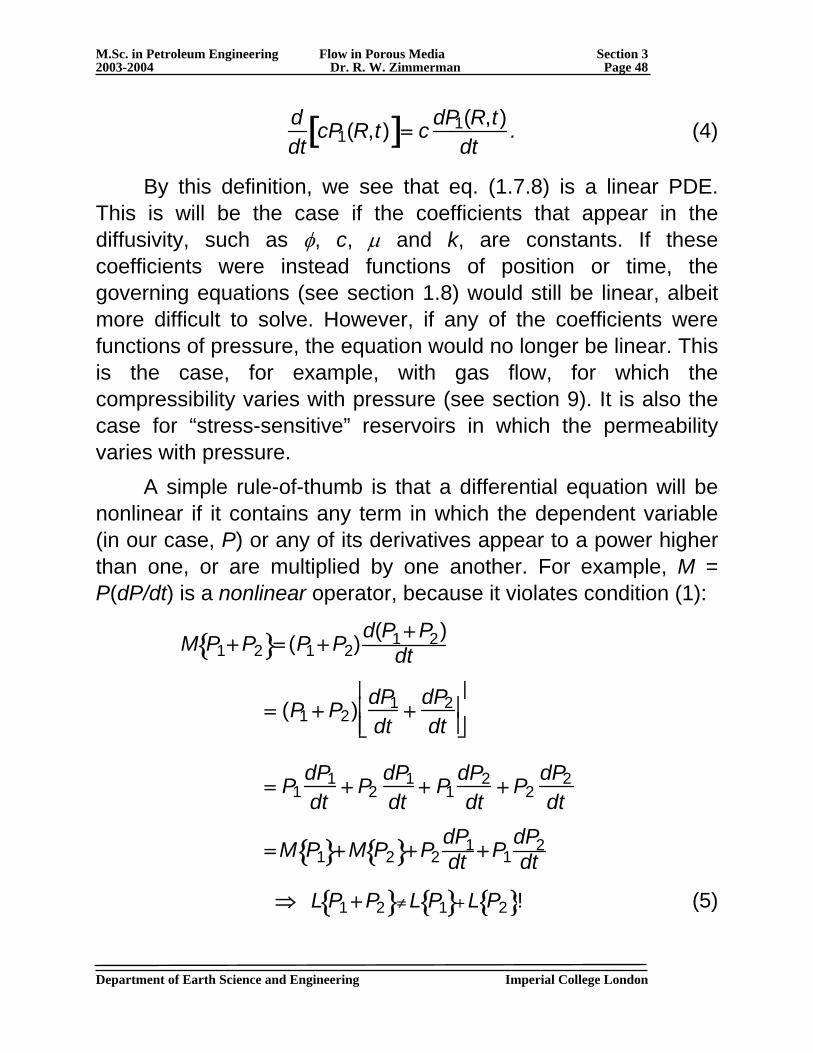
By this definition, we see that eq. (1.7.8) is a linear PDE. This is will be the case if the coefficients that appear in the diffusivity, such as φ, c, μ and k, are constants. If these coefficients were instead functions of position or time, the governing equations (see section 1.8) would still be linear, albeit more difficult to solve. However, if any of the coefficients were functions of pressure, the equation would no longer be linear. This is the case, for example, with gas flow, for which the compressibility varies with pressure (see section 9). It is also the case for “stress-sensitive” reservoirs in which the permeability varies with pressure. A simple rule-of-thumb is that a differential equation will be nonlinear if it contains any term in which the dependent variable (in our case, P) or any of its derivatives appear to a power higher than one, or are multiplied by one another. For example, M = P(dP/dt) is a nonlinear operator, because it violates condition (1):
M P1+ P2{ }= (P1 + P2)d(P1 + P2)
dt
= (P1 + P2) dP1
dt+
dP2dt
⎡
⎣ ⎢ ⎢
⎤
⎦ ⎥ ⎥
= P1
dP1dt
+ P2dP1dt
+ P1dP2dt
+ P2dP2dt
= M P1{ }+ M P2{ }+ P2
dP1dt + P1
dP2dt
⇒ L P1 + P2{ }≠ L P1{ }+ L P2{ }! (5)
Department of Earth Science and Engineering Imperial College London
M.Sc. in Petroleum Engineering Flow in Porous Media Section 3 2003-2004 Dr. R. W. Zimmerman Page 49
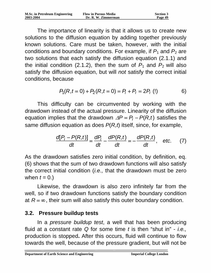
The importance of linearity is that it allows us to create new solutions to the diffusion equation by adding together previously known solutions. Care must be taken, however, with the initial conditions and boundary conditions. For example, if P1 and P2 are two solutions that each satisfy the diffusion equation (2.1.1) and the initial condition (2.1.2), then the sum of P1 and P2 will also satisfy the diffusion equation, but will not satisfy the correct initial conditions, because
P1(R,t = 0) + P2(R,t = 0) = Pi + Pi = 2Pi (!) 6)
This difficulty can be circumvented by working with the drawdown instead of the actual pressure. Linearity of the diffusion equation implies that the drawdown ΔP = Pi − P(R,t ) satisfies the same diffusion equation as does P(R,t) itself, since, for example,
d[Pi − P(R,t )]
dt=
dPidt
−dP(R,t )
dt= −
dP(R,t)dt
, etc. (7)
As the drawdown satisfies zero initial condition, by definition, eq. (6) shows that the sum of two drawdown functions will also satisfy the correct initial condition (i.e., that the drawdown must be zero when t = 0.) Likewise, the drawdown is also zero infinitely far from the well, so if two drawdown functions satisfy the boundary condition at R = ∞ , their sum will also satisfy this outer boundary condition.
3.2. Pressure buildup tests In a pressure buildup test, a well that has been producing fluid at a constant rate Q for some time t is then “shut in” - i.e., production is stopped. After this occurs, fluid will continue to flow towards the well, because of the pressure gradient, but will not be
Department of Earth Science and Engineering Imperial College London
M.Sc. in Petroleum Engineering Flow in Porous Media Section 3 2003-2004 Dr. R. W. Zimmerman Page 50
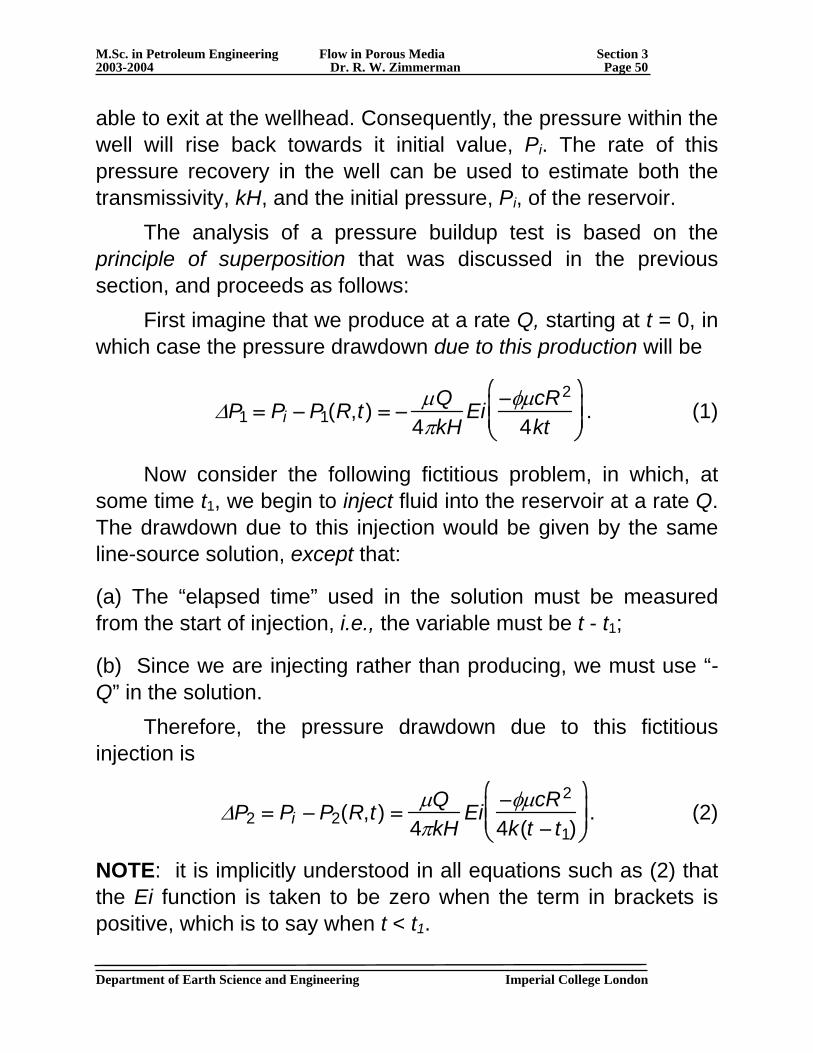
able to exit at the wellhead. Consequently, the pressure within the well will rise back towards it initial value, Pi. The rate of this pressure recovery in the well can be used to estimate both the transmissivity, kH, and the initial pressure, Pi, of the reservoir. The analysis of a pressure buildup test is based on the principle of superposition that was discussed in the previous section, and proceeds as follows: First imagine that we produce at a rate Q, starting at t = 0, in which case the pressure drawdown due to this production will be
ΔP1 = Pi − P1(R,t) = −
μQ4πkH
Ei −φμcR2
4kt
⎛
⎝ ⎜ ⎜
⎞
⎠ ⎟ ⎟ . (1)
Now consider the following fictitious problem, in which, at some time t1, we begin to inject fluid into the reservoir at a rate Q. The drawdown due to this injection would be given by the same line-source solution, except that:
(a) The “elapsed time” used in the solution must be measured from the start of injection, i.e., the variable must be t - t1;
(b) Since we are injecting rather than producing, we must use “-Q” in the solution. Therefore, the pressure drawdown due to this fictitious injection is
ΔP2 = Pi − P2(R,t) =
μQ4πkH
Ei −φμcR2
4k(t − t1)
⎛
⎝ ⎜ ⎜
⎞
⎠ ⎟ ⎟ . (2)
NOTE: it is implicitly understood in all equations such as (2) that the Ei function is taken to be zero when the term in brackets is positive, which is to say when t < t1.
Department of Earth Science and Engineering Imperial College London
M.Sc. in Petroleum Engineering Flow in Porous Media Section 3 2003-2004 Dr. R. W. Zimmerman Page 51
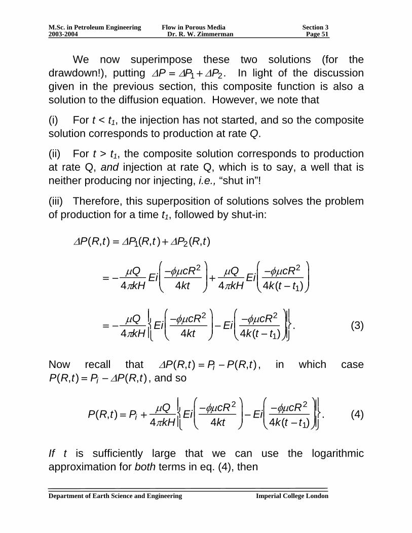
We now superimpose these two solutions (for the drawdown!), putting ΔP = ΔP1 + ΔP2. In light of the discussion given in the previous section, this composite function is also a solution to the diffusion equation. However, we note that
(i) For t < t1, the injection has not started, and so the composite solution corresponds to production at rate Q.
(ii) For t > t1, the composite solution corresponds to production at rate Q, and injection at rate Q, which is to say, a well that is neither producing nor injecting, i.e., “shut in”!
(iii) Therefore, this superposition of solutions solves the problem of production for a time t1, followed by shut-in:
ΔP(R,t) = ΔP1(R,t ) + ΔP2(R,t)
= −
μQ4πkH
Ei −φμcR2
4kt
⎛
⎝ ⎜ ⎜
⎞
⎠ ⎟ ⎟ +
μQ4πkH
Ei −φμcR2
4k(t − t1)
⎛
⎝ ⎜ ⎜
⎞
⎠ ⎟ ⎟
= −
μQ4πkH
Ei −φμcR2
4kt
⎛
⎝ ⎜ ⎜
⎞
⎠ ⎟ ⎟ − Ei −φμcR2
4k(t − t1)
⎛
⎝ ⎜ ⎜
⎞
⎠ ⎟ ⎟
⎧ ⎨ ⎪
⎩ ⎪
⎫ ⎬ ⎪
⎭ ⎪ . (3)
Now recall that ΔP(R,t) = Pi − P(R,t) , in which case P(R,t) = Pi − ΔP(R,t) , and so
P(R,t) = Pi +
μQ4πkH
Ei −φμcR2
4kt
⎛
⎝ ⎜ ⎜
⎞
⎠ ⎟ ⎟ − Ei −φμcR2
4k(t − t1)
⎛
⎝ ⎜ ⎜
⎞
⎠ ⎟ ⎟
⎧ ⎨ ⎪
⎩ ⎪
⎫ ⎬ ⎪
⎭ ⎪ . (4)
If t is sufficiently large that we can use the logarithmic approximation for both terms in eq. (4), then
Department of Earth Science and Engineering Imperial College London
M.Sc. in Petroleum Engineering Flow in Porous Media Section 3 2003-2004 Dr. R. W. Zimmerman Page 52
P(R,t) = Pi −
μQ4πkH
lnt + ln 2.246kφμcR2
⎛
⎝ ⎜ ⎜
⎞
⎠ ⎟ ⎟ − ln(t − t1) − ln 2.246k
φμcR2
⎛
⎝ ⎜ ⎜
⎞
⎠ ⎟ ⎟
⎧ ⎨ ⎪
⎩ ⎪
⎫ ⎬ ⎪
⎭ ⎪
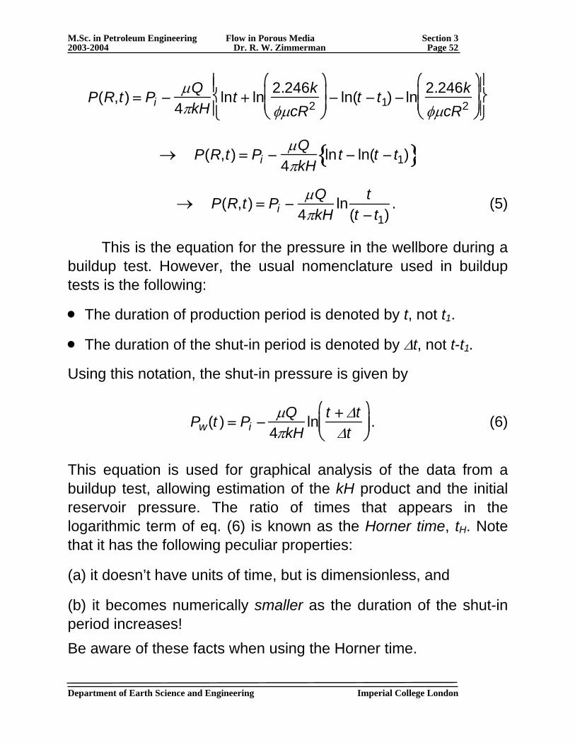
→ P(R,t) = Pi −
μQ4πkH
ln t − ln(t − t1){ }
→ P(R,t) = Pi −
μQ4πkH
ln t(t − t1)
. (5)
This is the equation for the pressure in the wellbore during a buildup test. However, the usual nomenclature used in buildup tests is the following:
• The duration of production period is denoted by t, not t1.
• The duration of the shut-in period is denoted by Δt, not t-t1.
Using this notation, the shut-in pressure is given by
Pw(t ) = Pi −
μQ4πkH
ln t + ΔtΔt
⎛
⎝ ⎜ ⎜
⎞
⎠ ⎟ ⎟ . (6)
This equation is used for graphical analysis of the data from a buildup test, allowing estimation of the kH product and the initial reservoir pressure. The ratio of times that appears in the logarithmic term of eq. (6) is known as the Horner time, tH. Note that it has the following peculiar properties:
(a) it doesn’t have units of time, but is dimensionless, and
(b) it becomes numerically smaller as the duration of the shut-in period increases! Be aware of these facts when using the Horner time.
Department of Earth Science and Engineering Imperial College London
M.Sc. in Petroleum Engineering Flow in Porous Media Section 3 2003-2004 Dr. R. W. Zimmerman Page 53
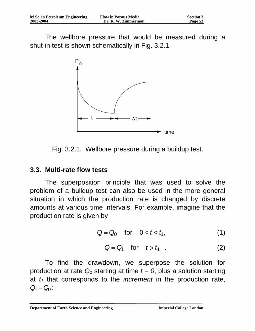
The wellbore pressure that would be measured during a shut-in test is shown schematically in Fig. 3.2.1.
Pw
time
t Δt
Fig. 3.2.1. Wellbore pressure during a buildup test.
3.3. Multi-rate flow tests
The superposition principle that was used to solve the problem of a buildup test can also be used in the more general situation in which the production rate is changed by discrete amounts at various time intervals. For example, imagine that the production rate is given by
Q = Q0 for 0 < t < t1, (1)
Q = Q1 for t > t1 . (2)
To find the drawdown, we superpose the solution for production at rate Q0 starting at time t = 0, plus a solution starting at t1 that corresponds to the increment in the production rate, Q1 − Q0:
Department of Earth Science and Engineering Imperial College London
M.Sc. in Petroleum Engineering Flow in Porous Media Section 3 2003-2004 Dr. R. W. Zimmerman Page 54
ΔP(R,t) = −
μQ04πkH
Ei −φμcR2
4kt
⎛
⎝ ⎜ ⎜
⎞
⎠ ⎟ ⎟ −
μ(Q1 − Q0)4πkH
Ei −φμcR2
4k(t − t1)
⎛
⎝ ⎜ ⎜
⎞
⎠ ⎟ ⎟ . (3)
To verify that it is correct to use the flowrate increment, note that for t > t1, the first Ei function corresponds to a flowrate of Q0, and the second corresponds to a rate of Q1 − Q0, so the total flowrate is
Q(t > t1) = Q0 + (Q1 − Q0) = Q1. (4)
The drawdown in the general case in which flowrate Qi
commences at time ti can therefore be represented by
ΔP(R,t) =
−μQ04πkH
Ei −φμcR2
4kt
⎛
⎝ ⎜ ⎜
⎞
⎠ ⎟ ⎟ −
μ(Qi − Qi −1)4πkH
Ei −φμcR2
4k(t − ti )
⎛
⎝ ⎜ ⎜
⎞
⎠ ⎟ ⎟
i =1∑ . (5)
We can simplify the notation by defining the pressure drawdown per unit of flowrate, with production starting at t = 0, as ΔPQ(t). For the line-source in an infinite reservoir, this definition takes the form
ΔPQ (R,t) ≡
ΔP(R,t;Q)Q
≡−μ
4πkHEi −φμcR2
4kt
⎛
⎝ ⎜ ⎜
⎞
⎠ ⎟ ⎟ , (6)
with the understanding that ΔPQ(t) = 0 when t < 0.
Using definition (6), the drawdown in a multi-rate test can be written as
ΔP(R,t) = Q0ΔPQ (R,t) + (Qi − Qi −1)ΔPQ (R,t − ti )
i =1∑ . (7)
Department of Earth Science and Engineering Imperial College London
M.Sc. in Petroleum Engineering Flow in Porous Media Section 3 2003-2004 Dr. R. W. Zimmerman Page 55
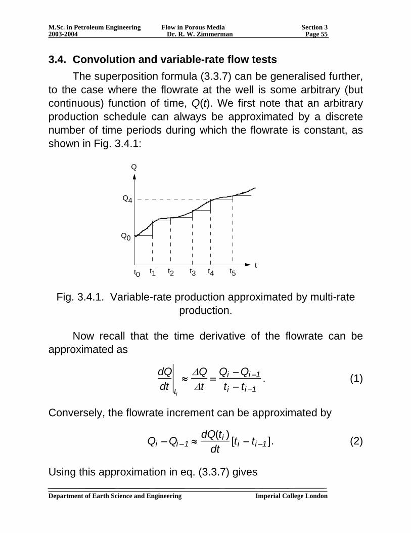
3.4. Convolution and variable-rate flow tests The superposition formula (3.3.7) can be generalised further, to the case where the flowrate at the well is some arbitrary (but continuous) function of time, Q(t). We first note that an arbitrary production schedule can always be approximated by a discrete number of time periods during which the flowrate is constant, as shown in Fig. 3.4.1:
Q
tt0 t1 t2 t3 t4 t5
Q0
Q4
Fig. 3.4.1. Variable-rate production approximated by multi-rate production.
Now recall that the time derivative of the flowrate can be approximated as
dQdt ti
≈ΔQΔt
=Qi − Qi −1ti − ti −1
. (1)
Conversely, the flowrate increment can be approximated by
Qi − Qi −1 ≈
dQ(ti )dt
[ti − ti −1 ]. (2)
Using this approximation in eq. (3.3.7) gives
Department of Earth Science and Engineering Imperial College London
M.Sc. in Petroleum Engineering Flow in Porous Media Section 3 2003-2004 Dr. R. W. Zimmerman Page 56
ΔP(R,t) = Q0ΔPQ (R,t) +
dQ(ti )dt
ΔPQ (R,t − ti )i =1∑ [ti − t i−1 ]. (3)
We now simplify the notation by rewriting eq. (3) in the following equivalent form:
ΔP(R,t) = Q0ΔPQ (R,t) + ′ Q (ti )ΔPQ (R,t − ti )
i =1∑ Δt i . (4)
As we make each time increment smaller, approximation (1) becomes more accurate, and the “step-function” approximation to Q(t) also becomes more accurate. In the limit as each time increment goes to zero, the errors due to these approximations will vanish. But as the time increments get smaller, the series in eq. (4) becomes an integral with respect to ti:
ΔP(R,t) = Q0ΔPQ (R,t) + ′ Q (ti )
ti =0
ti =t
∫ ΔPQ (R,t − ti )dti . (5)
The integral in eq. (5) ends at ti = t, because when ti > t, the function ΔPQ(t-ti) is zero, by definition. Physically, this reflects the fact that a change in flowrate that occurs at a time later than t cannot possibly have an effect on the drawdown at time t. Finally, we note that in the limit as each of the time increments become infinitely small, the finite number of times that we were denoting by ti evolve into a continuous variable, which we will denote by τ. The drawdown can then be written as
ΔP(R,t) = Q0ΔPQ (R,t) +
dQ(τ )dτ0
t∫ ΔPQ (R,t − τ )dτ . (6)
The integral in eq. (6) is known as a convolution integral. Formula (6) is also known as Duhamel’s principle, after the French
Department of Earth Science and Engineering Imperial College London

M.Sc. in Petroleum Engineering Flow in Porous Media Section 3 2003-2004 Dr. R. W. Zimmerman Page 57
physicist who first derived this equation in 1833 (in the context of solving heat conduction problems).
The importance of eq. (6) is that it allows us to find the drawdown for any production schedule, by merely performing a single integral utilising the “constant-flowrate” solution. The principle also works for other boundary-value problems that are governed by a linear PDE. For example, if we have a reservoir with, say, a closed outer boundary (see section 6), then we need only to find the solution for the case of constant flowrate in a reservoir with a closed outer boundary; the solution for a variable flowrate then follows from eq. (6), with the constant-flowrate solution playing the role of the function ΔPQ.
Another form of the convolution integral that is sometimes more convenient to use can be derived by applying integration-by-parts to the integral in (6). First, recall that the general expression for integration by parts is
f (τ ) dg(τ )
dτ0
t∫ dτ = f (τ )g(τ )]0
t− g(τ )df (τ )
dτ0
t∫ dτ . (7)
We now put f (τ ) = ΔPQ (R,t − τ ) and g(τ ) = Q(τ ), in which case (6) becomes
ΔP(R,t) = Q0ΔPQ (R,t) + Q(τ )ΔPQ (R,t − τ )]0t
− Q(τ ) dΔPQ (R,t − τ )dτ0
t∫ dτ
= Q0ΔPQ (R,t) + Q(t)ΔPQ (R,0) − Q(0)ΔPQ (R,t)
− Q(τ ) dΔPQ (R,t − τ )dτ0
t∫ dτ.
(8)
Department of Earth Science and Engineering Imperial College London
M.Sc. in Petroleum Engineering Flow in Porous Media Section 3 2003-2004 Dr. R. W. Zimmerman Page 58
But Q(0) = Q0, by definition, so the first and third terms on the right cancel out. And ΔPQ (R,0) is the drawdown at time zero, which must be zero, so the second term drops out.
Using the chain rule we can see that
dΔPQ (R,t − τ )
dτ=
−dΔPQ (R,t − τ )dt
, (9)
in which case (8) can finally be written as
ΔP(R,t) = Q(τ )
dΔPQ (R,t − τ )dt0
t∫ dτ . (10)
______________________________________________
Tutorial Sheet 3:
(1) Which, if any, of the following differential equations are linear, and why (or why not)?
(a) d2ydx2
+ y dydx
+ y = 0 .
(b) d2ydx2
+ x dydx
+ y = 0.
(c) d2ydx2
+ x dydx
+ xy = 0.
(2) What would be the wellbore pressure in a well in an infinite reservoir, if the production rate increases linearly as a function of time according to Q(t) = Q*t / t*, where Q* and t* are constants? Use convolution, in the form of either (3.4.6) or (3.4.10), and recall that ΔPQ(R,t) for a well in an infinite reservoir is given by eq. (3.3.6).
Department of Earth Science and Engineering Imperial College London
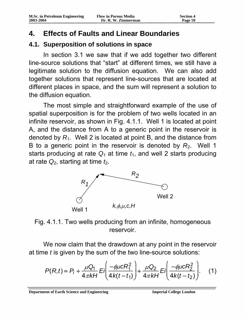
M.Sc. in Petroleum Engineering Flow in Porous Media Section 4 2003-2004 Dr. R. W. Zimmerman Page 59
Department of Earth Science and Engineering Imperial College London
4. Effects of Faults and Linear Boundaries 4.1. Superposition of solutions in space In section 3.1 we saw that if we add together two different line-source solutions that “start” at different times, we still have a legitimate solution to the diffusion equation. We can also add together solutions that represent line-sources that are located at different places in space, and the sum will represent a solution to the diffusion equation. The most simple and straightforward example of the use of spatial superposition is for the problem of two wells located in an infinite reservoir, as shown in Fig. 4.1.1. Well 1 is located at point A, and the distance from A to a generic point in the reservoir is denoted by R1. Well 2 is located at point B, and the distance from B to a generic point in the reservoir is denoted by R2. Well 1 starts producing at rate Q1 at time t1, and well 2 starts producing at rate Q2, starting at time t2.
k,φ,μ,c,H
R1
Well 1
Well 2
R2
Fig. 4.1.1. Two wells producing from an infinite, homogeneous reservoir.
We now claim that the drawdown at any point in the reservoir at time t is given by the sum of the two line-source solutions:
P(R,t) = Pi +
μQ14πkH
Ei−φμcR1
2
4k(t − t1)
⎛
⎝ ⎜ ⎜
⎞
⎠ ⎟ ⎟ +
μQ24π kH
Ei−φμcR2
2
4k(t − t2)
⎛
⎝ ⎜ ⎜
⎞
⎠ ⎟ ⎟ . (1)
M.Sc. in Petroleum Engineering Flow in Porous Media Section 4 2003-2004 Dr. R. W. Zimmerman Page 60
Department of Earth Science and Engineering Imperial College London
To prove that this is indeed the proper solution to this problem, we note that: (1) The line-source solution for well 1 satisfies the diffusion equation at all points in the reservoir (except at R1 = 0, where it gives an “infinite” drawdown), and at all times. Similarly for the second line-source solution. Hence, their sum satisfies the diffusion equation at all times, and at all points except R1 = 0 and R2 = 0. But these two points are not actually located in the reservoir, so we don’t care that the diffusion equation is not satisfied there!
(2) Both line-source solutions satisfy the initial condition of zero drawdown, so their sum also satisfies this initial condition.
(3) Both line-source solutions satisfy the far-field boundary condition that the drawdown is zero “at infinity”, so their sum also satisfies this boundary condition, i.e.,
P(R → ∞,t) = Pi +
μQ4π kH
Ei −∞( )+μQ
4π kHEi −∞( )= Pi , (2)
because, as can be seen from Table 2.1.1, Ei(-x) goes to zero as x becomes very large.
Hence, it seems that the drawdown given by eq. (1) is the correct solution for the two-well problem. Obviously, spatial superposition can be used for any number of wells.
The principle of superposition can also be used in conjunction with the concept of “fictitious” wells, or “image” wells, to solve problems such as finding the effect of a nearby impermeable fault, as explained in the next section.
M.Sc. in Petroleum Engineering Flow in Porous Media Section 4 2003-2004 Dr. R. W. Zimmerman Page 61
Department of Earth Science and Engineering Imperial College London
4.2. Effect of an impermeable vertical fault Hydrocarbon reservoirs are often transected by numerous faults, many of which are nearly vertical. Due to mineral deposition on the fault surfaces, accumulation of fault gouge, and other geological processes, faults are often impermeable to flow. In order to properly interpret the results of well tests, it is important to understand the effect that an impermeable linear boundary will have on a drawdown test. It is therefore desirable to find the solution for the problem of constant-rate production from a well located in an infinite, homogeneous reservoir that is bounded on one side by a vertical fault of infinite extent that is impermeable to flow. This solution can easily be found from the Theis solution for a well in an infinite (unbounded) reservoir, by using the principle of superposition. Consider a well located at a perpendicular distance (i.e., nearest distance) d from an impermeable fault, which appears in planview as a straight line that extends infinitely far in both directions, as in Fig. 4.2.1. This well produces fluid at a constant rate Q, starting at t = 0. Now imagine a fictitious “image well” that is situated as the “mirror image” of the first well (i.e., at a distance d on the other side of the fault) which also produces at rate Q starting at t = 0, as in Fig. 4.2.1. By the symmetry of this situation, no fluid will cross the plane of the fault. Hence, this plane will effectively act as a no-flow boundary. We therefore have found the solution for a well near an impermeable fault!
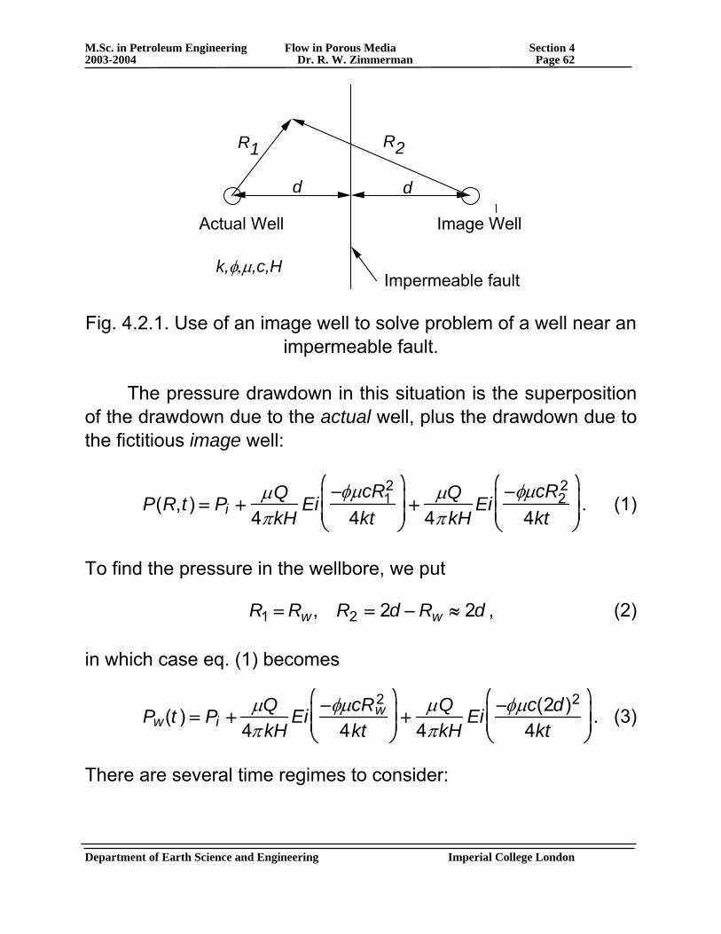
M.Sc. in Petroleum Engineering Flow in Porous Media Section 4 2003-2004 Dr. R. W. Zimmerman Page 62
Department of Earth Science and Engineering Imperial College London
Impermeable faultk,φ,μ,c,H
R1
Actual Well Image Well
R2
d d
Fig. 4.2.1. Use of an image well to solve problem of a well near an impermeable fault.
The pressure drawdown in this situation is the superposition of the drawdown due to the actual well, plus the drawdown due to the fictitious image well:
P(R,t) = Pi +
μQ4πkH
Ei−φμcR1
2
4kt
⎛
⎝ ⎜ ⎜
⎞
⎠ ⎟ ⎟ +
μQ4π kH
Ei−φμcR2
2
4kt
⎛
⎝ ⎜ ⎜
⎞
⎠ ⎟ ⎟ . (1)
To find the pressure in the wellbore, we put
R1 = Rw , R2 = 2d − Rw ≈ 2d , (2)
in which case eq. (1) becomes
Pw(t ) = Pi +
μQ4π kH
Ei −φμcRw2
4kt
⎛
⎝ ⎜ ⎜
⎞
⎠ ⎟ ⎟ +
μQ4πkH
Ei −φμc(2d)2
4kt
⎛
⎝ ⎜ ⎜
⎞
⎠ ⎟ ⎟ . (3)
There are several time regimes to consider:
M.Sc. in Petroleum Engineering Flow in Porous Media Section 4 2003-2004 Dr. R. W. Zimmerman Page 63
Department of Earth Science and Engineering Imperial College London
(i) There is an early time regime, during which the logarithmic approximation is not yet valid for the actual well solution (nor for the image-well solution). From eq. (2.4.7) this regime is defined by
t <
25φμcRw2
k, or tDw < 25 . (4)
• In this regime, we would have to use the full infinite series expansion for the exponential integral function.
• However, we saw in Section 2.3 that the duration of this regime is usually very short, so there is no need for us to study it further.
(ii) There is another regime in which the logarithmic approximation can be used for the well solution, but the drawdown in the wellbore due to the image solution is still negligible. The start of this regime is defined by eq. (4), i.e.,
t >
25φμcRw2
k, or tDw > 25 . (5)
This regime ends when the front edge of the pressure pulse from the image well reaches the actual well (which is a distance 2d away). We can consider that this occurs when the second Ei function in eq. (3) reaches, say, 0.01.
According to Table 2.1.1, this occurs when the argument of the Ei function reaches about 3.3. Therefore, the upper limit of this time regime is defined by
M.Sc. in Petroleum Engineering Flow in Porous Media Section 4 2003-2004 Dr. R. W. Zimmerman Page 64
Department of Earth Science and Engineering Imperial College London
t <
0.3φμcd2
k, or tDw < 0.3(d / Rw )2. (6)
• In this regime, the pressure in the well is given by
Pw(t ) = Pi −
μQ4π kH
ln 2.246ktφμcRw
2
⎛
⎝ ⎜ ⎜
⎞
⎠ ⎟ ⎟ . (7)
i.e., this is the drawdown that would occur in the absence of the fault, because in this time regime the actual pressure pulse has not yet had time to travel to the fault and reflect back to the wellbore (where it can be detected).
• In particular, during this regime the slope of the wellbore pressure curve on a semi-log plot will be
dPwd ln t
=ΔPwΔ ln t
=−μQ4πkH
. (8)
(iii) There is a late time regime during which the logarithmic approximation is valid for both the actual well solution, and the image well solution.
• This regime is defined by
t >
25φμc(2d)2
k, or tDw > 100(d /Rw)2. (9)
• In this regime, the pressure in the well is
Pw(t ) = Pi −
μQ4π kH
ln 2.246ktφμcRw
2
⎛
⎝ ⎜ ⎜
⎞
⎠ ⎟ ⎟ −
μQ4πkH
ln 2.246ktφμc(2d)2
⎛
⎝ ⎜ ⎜
⎞
⎠ ⎟ ⎟
M.Sc. in Petroleum Engineering Flow in Porous Media Section 4 2003-2004 Dr. R. W. Zimmerman Page 65
Department of Earth Science and Engineering Imperial College London
= Pi −
μQ4πkH
ln t + ln 2.246kφμcRw
2
⎛
⎝ ⎜ ⎜
⎞
⎠ ⎟ ⎟ + ln t + ln 2.246k
φμc4d2
⎛
⎝ ⎜ ⎜
⎞
⎠ ⎟ ⎟
⎡
⎣ ⎢ ⎢
⎤
⎦ ⎥ ⎥
= Pi −
μQ4πkH
2ln t + ln 2.246kφμcRw
2
⎛
⎝ ⎜ ⎜
⎞
⎠ ⎟ ⎟ + ln 2.246k
φμc4d2
⎛
⎝ ⎜ ⎜
⎞
⎠ ⎟ ⎟
⎡
⎣ ⎢ ⎢
⎤
⎦ ⎥ ⎥ . (10)
This equation will also yield a straight line on a plot of Pw vs. lnt, but with a slope that is twice that of the earlier slope:
dPwd ln t
=ΔPwΔ ln t
=−2μQ4πkH
=−μQ2πkH
. (11)
→ The occurrence of a doubling of the slope of Pw vs. lnt is an indication of a nearby impermeable boundary! Moreover, the distance from the production well to the fault can be estimated from the transition time between the regime when eq. (7) is applicable, to the regime when eq. (10) becomes applicable (see module 2.1.6).
Physical Explanation: Because of the impermeable boundary, oil is being produced from a “semi-infinite” reservoir, rather than an infinite reservoir. Hence, we expect that only half as much oil will be produced, for a given wellbore pressure. So, in order to maintain a constant flowrate, we must double the pressure drawdown!
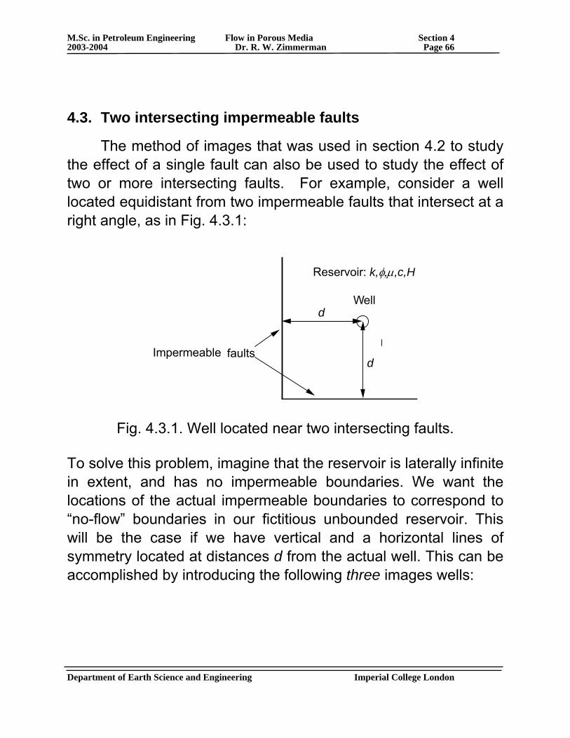
M.Sc. in Petroleum Engineering Flow in Porous Media Section 4 2003-2004 Dr. R. W. Zimmerman Page 66
Department of Earth Science and Engineering Imperial College London
4.3. Two intersecting impermeable faults
The method of images that was used in section 4.2 to study the effect of a single fault can also be used to study the effect of two or more intersecting faults. For example, consider a well located equidistant from two impermeable faults that intersect at a right angle, as in Fig. 4.3.1:
faults
Reservoir: k,φ,μ,c,H
Welld
Impermeabled
Fig. 4.3.1. Well located near two intersecting faults.
To solve this problem, imagine that the reservoir is laterally infinite in extent, and has no impermeable boundaries. We want the locations of the actual impermeable boundaries to correspond to “no-flow” boundaries in our fictitious unbounded reservoir. This will be the case if we have vertical and a horizontal lines of symmetry located at distances d from the actual well. This can be accomplished by introducing the following three images wells:
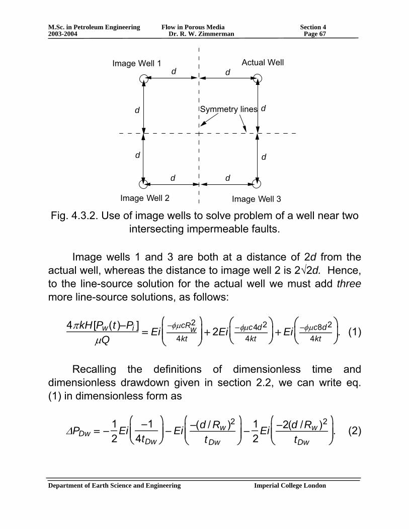
M.Sc. in Petroleum Engineering Flow in Porous Media Section 4 2003-2004 Dr. R. W. Zimmerman Page 67
Department of Earth Science and Engineering Imperial College London
Actual WellImage Well 1d d
Image Well 2 Image Well 3
d
d
d d
d
dSymmetry lines
Fig. 4.3.2. Use of image wells to solve problem of a well near two
intersecting impermeable faults.
Image wells 1 and 3 are both at a distance of 2d from the actual well, whereas the distance to image well 2 is 2√2d. Hence, to the line-source solution for the actual well we must add three more line-source solutions, as follows:
4πkH [Pw(t)−Pi ]μQ
= Ei−φμcRw
2
4kt
⎛
⎝ ⎜ ⎜
⎞
⎠ ⎟ ⎟ + 2Ei −φμc4d2
4kt
⎛
⎝ ⎜
⎞
⎠ ⎟ + Ei −φμc8d2
4kt
⎛
⎝ ⎜
⎞
⎠ ⎟ . (1)
Recalling the definitions of dimensionless time and dimensionless drawdown given in section 2.2, we can write eq. (1) in dimensionless form as
ΔPDw = −
12
Ei −14tDw
⎛
⎝ ⎜ ⎜
⎞
⎠ ⎟ ⎟ − Ei −(d / Rw )2
tDw
⎛
⎝ ⎜ ⎜
⎞
⎠ ⎟ ⎟ −
12
Ei −2(d /Rw )2
tDw
⎛
⎝ ⎜ ⎜
⎞
⎠ ⎟ ⎟ . (2)
M.Sc. in Petroleum Engineering Flow in Porous Media Section 4 2003-2004 Dr. R. W. Zimmerman Page 68
Department of Earth Science and Engineering Imperial College London
The wellbore pressure will exhibit an early stage in which the effect of the image wells is not yet apparent, and the semi-log slope of the wellbore pressure vs. time curve will be -Qμ/4πkH. Eventually, at a sufficiently long time such that the drawdown in the actual well due to production from all four wells can be approximated by the logarithmic approximation, the semi-log slope will be four times greater in magnitude, i.e., -Qμ/πkH. Note that application of the method of images is not quite as simple as saying “if we had one impermeable boundary we added in one image well, so for two impermeable boundaries we add two image wells”; this statement might seem logical, but it is not correct. The trick is to place image wells so as to create a fictitious unbounded reservoir that has the proper symmetry in its flow field. Several other examples of the use of the method of images (two infinite parallel faults, two faults intersecting at 45o, etc.) can be found in the book Well Testing in Heterogeneous Formations, by T. D. Streltsova (Wiley, 1988).
4.4. Linear constant-pressure boundaries Another situation that sometimes arises in reservoirs is that of a linear constant-pressure boundary. This boundary may, for example, be formed by a gas cap that borders a slightly dipping oil reservoir. The effect that such a boundary has on a drawdown test can also be studied by using the method of images. Imagine an image well, located as in Fig. 4.2.1, but injecting fluid at a rate Q. Again, we “ignore” the actual constant-pressure boundary, and assume that the actual well and the image well are located in an infinite reservoir. By superposition, the drawdown at a generic location in the reservoir will be
M.Sc. in Petroleum Engineering Flow in Porous Media Section 4 2003-2004 Dr. R. W. Zimmerman Page 69
Department of Earth Science and Engineering Imperial College London
P(R,t) = Pi +
μQ4πkH
Ei−φμcR1
2
4kt
⎛
⎝ ⎜ ⎜
⎞
⎠ ⎟ ⎟ −
μQ4π kH
Ei−φμcR2
2
4kt
⎛
⎝ ⎜ ⎜
⎞
⎠ ⎟ ⎟ . (1)
Now consider a point on the mid-plane between the two wells. At such a point, R1 = R2, and so eq. (1) gives
P(midplane,t) = Pi +
μQ4π kH
Ei−φμcR1
2
4kt
⎛
⎝ ⎜ ⎜
⎞
⎠ ⎟ ⎟ − Ei
−φμcR12
4kt
⎛
⎝ ⎜ ⎜
⎞
⎠ ⎟ ⎟
⎡
⎣ ⎢ ⎢
⎤
⎦ ⎥ ⎥ .
= Pi for all t, (2)
proving that the midplane is indeed a constant-pressure boundary. Now, consider the pressure drawdown in the actual well, which is found by setting R1 = Rw and R2 = 2d - Rw = 2d:
P(R,t) = Pi +
μQ4πkH
Ei −φμcRw2
4kt
⎛
⎝ ⎜ ⎜
⎞
⎠ ⎟ ⎟ −
μQ4π kH
Ei −φμc(2d)2
4kt
⎛
⎝ ⎜ ⎜
⎞
⎠ ⎟ ⎟ . (3)
● Again, aside from a very-early time regime defined by eq. (4.2.4), which we ignore, we have, in analogy with eqs. (4.2.5,6), a regime defined by tDw > 25 and
t <
0.3φμcd2
k, or tDw < 0.3(d / Rw )2, (4)
during which the effect of the image well has not yet been felt in the actual well, and so the pressure in the well is given by
Pw(t ) = Pi −
μQ4π kH
ln 2.246ktφμcRw
2
⎛
⎝ ⎜ ⎜
⎞
⎠ ⎟ ⎟ . (5)
M.Sc. in Petroleum Engineering Flow in Porous Media Section 4 2003-2004 Dr. R. W. Zimmerman Page 70
Department of Earth Science and Engineering Imperial College London
● There is a late-time regime during which the logarithmic approximation is valid (in the production well) for both the actual line-source solution and the image line-source solution. In analogy with eq. (4.2.9), this regime is defined by
t >
25φμc(2d)2
k, or tDw > 100(d /Rw)2. (6)
● In this regime, the pressure in the well is given by
Pw(t ) = Pi −
μQ4π kH
ln 2.246ktφμcRw
2
⎛
⎝ ⎜ ⎜
⎞
⎠ ⎟ ⎟ +
μQ4πkH
ln 2.246ktφμc(2d )2
⎛
⎝ ⎜ ⎜
⎞
⎠ ⎟ ⎟
= Pi −
μQ4πkH
ln t + ln 2.246kφμcRw
2
⎛
⎝ ⎜ ⎜
⎞
⎠ ⎟ ⎟ − ln t − ln 2.246k
φμc(2d)2⎛
⎝ ⎜ ⎜
⎞
⎠ ⎟ ⎟
⎡
⎣ ⎢ ⎢
⎤
⎦ ⎥ ⎥
= Pi −
μQ4πkH
ln 2.246kφμc
⎛
⎝ ⎜ ⎜
⎞
⎠ ⎟ ⎟ − ln(Rw
2 ) − ln 2.246kφμc
⎛
⎝ ⎜ ⎜
⎞
⎠ ⎟ ⎟ + ln (2d )2{ }
⎡
⎣ ⎢ ⎢
⎤
⎦ ⎥ ⎥
= Pi −
μQ4πkH
ln (2d / Rw )2{ } = Pi −
μQ2π kH
ln 2dRw
⎛
⎝ ⎜ ⎜
⎞
⎠ ⎟ ⎟ . (7)
In this case, the pressure in the production well eventually stabilises to a constant value. The steady-state value of the drawdown is a function of the dimensionless distance to the boundary (relative to the wellbore radius).
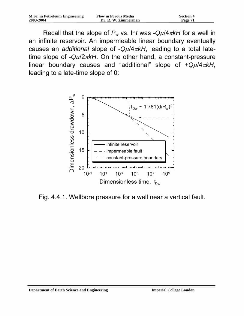
M.Sc. in Petroleum Engineering Flow in Porous Media Section 4 2003-2004 Dr. R. W. Zimmerman Page 71
Department of Earth Science and Engineering Imperial College London
Recall that the slope of Pw vs. lnt was -Qμ/4πkH for a well in an infinite reservoir. An impermeable linear boundary eventually causes an additional slope of -Qμ/4πkH, leading to a total late-time slope of -Qμ/2πkH. On the other hand, a constant-pressure linear boundary causes and “additional” slope of +Qμ/4πkH, leading to a late-time slope of 0:
0
5
10
15
2010-1 101 103 105 107 109
infinite reservoirimpermeable faultconstant-pressure boundary
Dim
ensi
onle
ss d
raw
dow
n, Δ
P w
Dimensionless time, tDw
tDw ~ 1.781(d/Rw)2
Fig. 4.4.1. Wellbore pressure for a well near a vertical fault.
M.Sc. in Petroleum Engineering Flow in Porous Media Section 4 2003-2004 Dr. R. W. Zimmerman Page 72
Department of Earth Science and Engineering Imperial College London
____________________________________________________ Tutorial Sheet 4:
(1) As explained in Section 4.2, a doubling of the slope on a semi-log plot of drawdown vs. time indicates the presence of an impermeable linear fault. The drawdown data can also be used to find the distance from the well to the fault, as follows. If we plot the data and then fit two straight lines through the early-time and late-time data, the time at which these lines intersect is called ′ t Dw . Show that the distance to the fault can then be found from the following equation:
d =0.749 ( ′ t Dw )1/2Rw .
(2) The curves in Fig. 4.4.1 were actually drawn for the case d/Rw = 200. What would the curves look like for the case of a fault located at a distance d = 400Rw?
(3) Consider a well located equidistant from two orthogonal boundaries, as in Fig. 4.3.1, but imagine that the boundaries are constant-pressure boundaries, rather than impermeable boundaries. How would you utilise the method of images to find the drawdown in this well?
M.Sc. in Petroleum Engineering Flow in Porous Media Section 5 2003-2004 Dr. R. W. Zimmerman Page 73
5. Inner (Wellbore) Boundary Conditions In the line-source solution that we have been discussing thus far, the effect of the borehole itself is actually ignored - the borehole is idealised as an infinitely-thin “line”. In this section, we will examine two physical phenomena associated with the borehole that necessitate a more detailed analysis of the diffusion equation. One of these phenomena is the existence of a zone of altered permeability around the borehole; the second is the effect of transient fluid storage within the borehole itself.
5.1. Wellbore skin concept - steady-state model The solutions to the diffusion equation that were presented in previous sections were all based on the assumption that the permeability of the reservoir is uniform in space. However, it is often the case that the rock immediately surrounding the wellbore has a lower permeability than the remainder of the reservoir, for various reasons: (1) Infiltration of drilling mud into the formation, which clogs up
the pores of the rock. (2) Swelling of clays in the formation due to contact with drilling
fluid. (3) Incomplete perforation of the casing, which causes the
flowpaths of the fluid to be constricted as they approach the wellbore. This has an effect that is similar to that caused by a low-permeability zone near the wellbore.
To account for these possibilities, we introduce the concept of “wellbore skin”, which can be thought of as a thin annular region surrounding the borehole in which the permeability ks is lower than that of the undamaged reservoir rock, as illustrated schematically in Fig. 5.1.1.
Department of Earth Science and Engineering Imperial College London
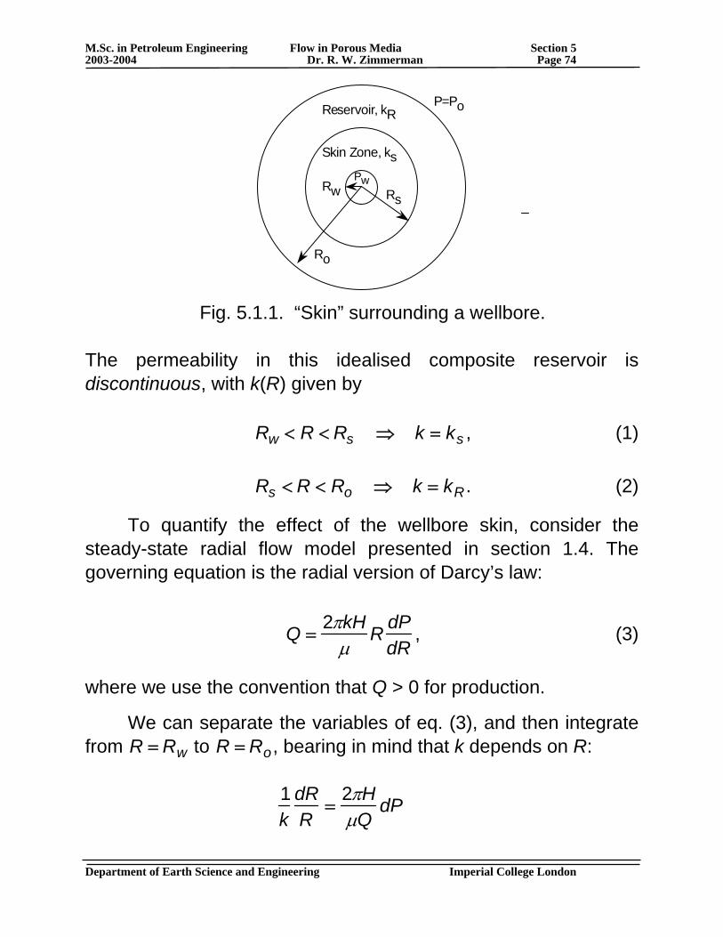
M.Sc. in Petroleum Engineering Flow in Porous Media Section 5 2003-2004 Dr. R. W. Zimmerman Page 74
Rw Rs
Ro
Reservoir, kR
Skin Zone, ks
P=Po
Pw
Fig. 5.1.1. “Skin” surrounding a wellbore.
The permeability in this idealised composite reservoir is discontinuous, with k(R) given by
Rw < R < Rs ⇒ k = ks , (1)
Rs < R < Ro ⇒ k = kR . (2)
To quantify the effect of the wellbore skin, consider the steady-state radial flow model presented in section 1.4. The governing equation is the radial version of Darcy’s law:
Q =
2πkHμ
R dPdR
, (3)
where we use the convention that Q > 0 for production.
We can separate the variables of eq. (3), and then integrate from R = Rw to R = Ro, bearing in mind that k depends on R:
1k
dRR
=2πHμQ
dP
Department of Earth Science and Engineering Imperial College London
M.Sc. in Petroleum Engineering Flow in Porous Media Section 5 2003-2004 Dr. R. W. Zimmerman Page 75
1ks
dRRRw
Rs
∫ +1
kR
dRRRs
Ro
∫ =2πHμQPw
Po
∫ dP
1ks
ln RsRw
+1
kRlnRo
Rs=
2πHμQ
(Po − Pw)
1kR
lnRoRs
+kRks
ln RsRw
⎡
⎣ ⎢ ⎢
⎤
⎦ ⎥ ⎥
=2πHμQ
(Po − Pw )
1kR
lnRoRs
+ ln RsRw
+kRks
ln RsRw
− ln RsRw
⎡
⎣ ⎢ ⎢
⎤
⎦ ⎥ ⎥
=2πHμQ
(Po − Pw)
1kR
ln RoRs
RsRw
⎛
⎝ ⎜ ⎜
⎞
⎠ ⎟ ⎟ +
kRks
− 1⎛
⎝ ⎜ ⎜
⎞
⎠ ⎟ ⎟ ln
RsRw
⎡
⎣ ⎢ ⎢
⎤
⎦ ⎥ ⎥
=2πHμQ
(Po − Pw )
→
2πkRH(Po − Pw )μQ
= ln RoRw
+kRks
− 1⎛
⎝ ⎜ ⎜
⎞
⎠ ⎟ ⎟ ln
RsRw
. (4)
Equation (4) is identical to eq. (1.4.3), except for the second term on the RHS. This excess dimensionless pressure drop, which is due to the presence of the skin effect, is denoted by s, i.e.,
2πkRH(Po − Pw )μQ
= ln RoRw
+ s . (5)
The effect of the skin is therefore to add an additional component to the pressure drawdown, over-and-above that which is due to the hydraulic resistance of the reservoir itself.
The dimensional form of the pressure drawdown in the well can be written as
Department of Earth Science and Engineering Imperial College London
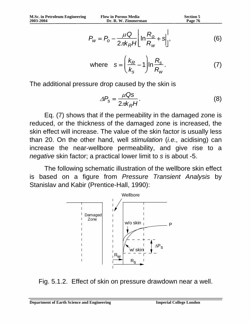
M.Sc. in Petroleum Engineering Flow in Porous Media Section 5 2003-2004 Dr. R. W. Zimmerman Page 76
Pw = Po −
μQ2πkRH
ln RoRw
+ s⎡
⎣ ⎢ ⎢
⎤
⎦ ⎥ ⎥ , (6)
where s =
kRks
− 1⎛
⎝ ⎜ ⎜
⎞
⎠ ⎟ ⎟ ln
RsRw
. (7)
The additional pressure drop caused by the skin is
ΔPs =
μQs2πkRH
. (8)
Eq. (7) shows that if the permeability in the damaged zone is reduced, or the thickness of the damaged zone is increased, the skin effect will increase. The value of the skin factor is usually less than 20. On the other hand, well stimulation (i.e., acidising) can increase the near-wellbore permeability, and give rise to a negative skin factor; a practical lower limit to s is about -5.
The following schematic illustration of the wellbore skin effect is based on a figure from Pressure Transient Analysis by Stanislav and Kabir (Prentice-Hall, 1990):
RwRs
Damaged Zone
Wellbore
P
ΔPs
w/o skin
w/ skin
Fig. 5.1.2. Effect of skin on pressure drawdown near a well.
Department of Earth Science and Engineering Imperial College London
M.Sc. in Petroleum Engineering Flow in Porous Media Section 5 2003-2004 Dr. R. W. Zimmerman Page 77
Another interpretation of the skin effect is based on the observation that the effect of skin is the same as the effect of having a smaller wellbore radius, i.e., it reduces the flow, for a given pressure drawdown. Hence, we can write eq. (6) as
Pw = Po −
μQ2πkRH
ln RoRw
− ln(e−s )⎡
⎣ ⎢ ⎢
⎤
⎦ ⎥ ⎥
= Po −
μQ2πkRH
ln Ro
Rwe −s
⎛
⎝ ⎜ ⎜
⎞
⎠ ⎟ ⎟
= Po −
μQ2πkRH
ln Ro
Rweff
⎛
⎝ ⎜ ⎜
⎞
⎠ ⎟ ⎟ , (9)
where Rweff = Rwe −s . (10)
Rweff can be thought of as the hypothetical wellbore radius (in an
undamaged formation) that would lead to the same drawdown as is actually observed in the well that is surrounded by the damaged formation.
[However, this interpretation is potentially misleading, because in general it is not correct to merely replace the actual wellbore radius with the effective radius given in eq. (10). This interpretation only applies to drawdown tests in an infinite reservoir.]
Department of Earth Science and Engineering Imperial College London
M.Sc. in Petroleum Engineering Flow in Porous Media Section 5 2003-2004 Dr. R. W. Zimmerman Page 78
5.2. Effect of skin on drawdown tests
The preceding derivation was carried out under the steady-state assumption. However, the thickness of the skin region is usually small, and so transient effects due to the skin region will die out rapidly. The time required for “transient effects” to die out within the skin region can be estimated using eq. (1.6.12), with the distance taken to be Rs:
ts =
(φμc)sRs2
4ks. (1)
If we assume reasonable values of the parameters, such as , , φ ≈ 10−1 μ ≈ 10−3 Pas c ≈ 10−9 /Pa, Rs ≈ 100 m, and
ks ≈ 10−15 m2, we find that ts ≈ 25s.
So, after a short period of time, the skin region will be in a quasi-steady regime. If the flowrate into the wellbore is constant, the pressure drop through the skin region will be constant. Therefore, it is usually assumed that, even during a transient well test, the effect of the skin is to contribute an additional pressure drop in the wellbore, as given by eq. (5.1.8). For example, the drawdown in an infinite reservoir producing at a constant rate, with a skin region around the wellbore, is found by subtracting the additional skin-related pressure drop given by eq. (5.1.8) from the usual line-source solution:
Pw = Pi −
μQ4πkH
−Ei φμcRw2
4kt
⎛
⎝ ⎜ ⎜
⎞
⎠ ⎟ ⎟ + 2s
⎡
⎣ ⎢ ⎢
⎤
⎦ ⎥ ⎥ , (2)
where we now revert to using k instead of kR to denote the reservoir permeability, since the permeability kS is absorbed into the skin factor, s. Department of Earth Science and Engineering Imperial College London
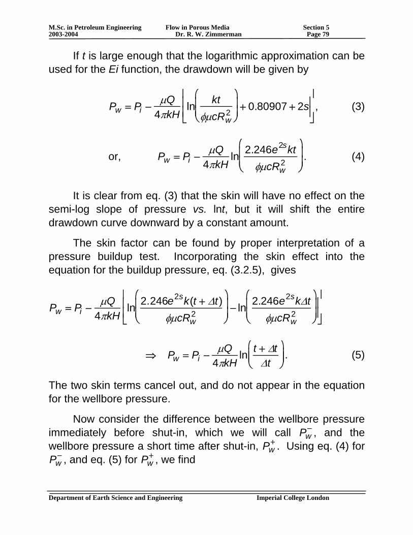
M.Sc. in Petroleum Engineering Flow in Porous Media Section 5 2003-2004 Dr. R. W. Zimmerman Page 79
If t is large enough that the logarithmic approximation can be used for the Ei function, the drawdown will be given by
Pw = Pi −
μQ4πkH
ln ktφμcRw
2
⎛
⎝ ⎜ ⎜
⎞
⎠ ⎟ ⎟ + 0.80907 + 2s
⎡
⎣ ⎢ ⎢
⎤
⎦ ⎥ ⎥ , (3)
or, Pw = Pi −
μQ4πkH
ln 2.246e2sktφμcRw
2
⎛
⎝ ⎜ ⎜
⎞
⎠ ⎟ ⎟ . (4)
It is clear from eq. (3) that the skin will have no effect on the semi-log slope of pressure vs. lnt, but it will shift the entire drawdown curve downward by a constant amount.
The skin factor can be found by proper interpretation of a pressure buildup test. Incorporating the skin effect into the equation for the buildup pressure, eq. (3.2.5), gives
Pw = Pi −
μQ4πkH
ln 2.246e2sk(t + Δt)φμcRw
2
⎛
⎝ ⎜ ⎜
⎞
⎠ ⎟ ⎟ − ln 2.246e2skΔt
φμcRw2
⎛
⎝ ⎜ ⎜
⎞
⎠ ⎟ ⎟
⎡
⎣ ⎢ ⎢
⎤
⎦ ⎥ ⎥
⇒ Pw = Pi −
μQ4πkH
ln t + ΔtΔt
⎛
⎝ ⎜ ⎜
⎞
⎠ ⎟ ⎟ . (5)
The two skin terms cancel out, and do not appear in the equation for the wellbore pressure.
Now consider the difference between the wellbore pressure immediately before shut-in, which we will call Pw
− , and the wellbore pressure a short time after shut-in, Pw
+ . Using eq. (4) for Pw
− , and eq. (5) for Pw+ , we find
Department of Earth Science and Engineering Imperial College London
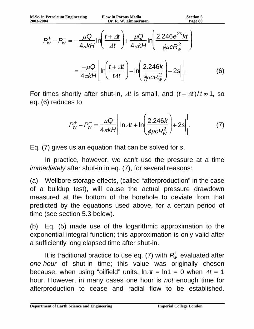
M.Sc. in Petroleum Engineering Flow in Porous Media Section 5 2003-2004 Dr. R. W. Zimmerman Page 80
Pw
+ − Pw− = −
μQ4πkH
ln t + ΔtΔt
⎛
⎝ ⎜ ⎜
⎞
⎠ ⎟ ⎟ +
μQ4πkH
ln 2.246e2sktφμcRw
2
⎛
⎝ ⎜ ⎜
⎞
⎠ ⎟ ⎟
=
−μQ4πkH
ln t + ΔttΔt
⎛
⎝ ⎜ ⎜
⎞
⎠ ⎟ ⎟ − ln 2.246k
φμcRw2
⎛
⎝ ⎜ ⎜
⎞
⎠ ⎟ ⎟ − 2s
⎡
⎣ ⎢ ⎢
⎤
⎦ ⎥ . (6) ⎥
For times shortly after shut-in, Δt is small, and (t + Δt ) / t ≈ 1, so eq. (6) reduces to
Pw
+ − Pw− =
μQ4πkH
lnΔt + ln 2.246kφμcRw
2
⎛
⎝ ⎜ ⎜
⎞
⎠ ⎟ ⎟ + 2s
⎡
⎣ ⎢ ⎢
⎤
⎦ ⎥ ⎥ . (7)
Eq. (7) gives us an equation that can be solved for s.
In practice, however, we can’t use the pressure at a time immediately after shut-in in eq. (7), for several reasons:
(a) Wellbore storage effects, (called “afterproduction” in the case of a buildup test), will cause the actual pressure drawdown measured at the bottom of the borehole to deviate from that predicted by the equations used above, for a certain period of time (see section 5.3 below).
(b) Eq. (5) made use of the logarithmic approximation to the exponential integral function; this approximation is only valid after a sufficiently long elapsed time after shut-in.
It is traditional practice to use eq. (7) with Pw+ evaluated after
one-hour of shut-in time; this value was originally chosen because, when using “oilfield” units, lnΔt = ln1 = 0 when Δt = 1 hour. However, in many cases one hour is not enough time for afterproduction to cease and radial flow to be established.
Department of Earth Science and Engineering Imperial College London
M.Sc. in Petroleum Engineering Flow in Porous Media Section 5 2003-2004 Dr. R. W. Zimmerman Page 81
Therefore, we must extrapolate the straight-line portion of the Horner plot back to Δt = 1 hour, and use that pressure for Pw
+ . Use of buildup data to estimate the skin factor will be illustrated in more detail in the Well Test Analysis module.
5.3. Wellbore storage phenomena The pressure drawdown is usually measured at the bottom of the borehole, whereas the flowrate is usually measured at the wellhead. The flowrate Q in our equations, however, refers to the sandface flowrate from the reservoir into the borehole. In a quasi-steady situation, the measured wellhead flowrate will be identical to the influx from the reservoir. Immediately after a change in flowrate, such as after the start of a drawdown test, or after shut-in, these two flowrates will be different. The difference is due to the fact that the fluid in the borehole is compressing (or expanding) due to the changing pressure to which it is subjected. For example, imagine that we begin to withdraw fluid at time t = 0 at rate Qwh that is measured at the wellhead. Initially, the fluid that flows at the wellhead is taken mainly from the wellbore itself; only gradually does this fluid begin to be supplied by the reservoir. Eventually, the fluid in the wellbore reaches a quasi-steady state, and all of the flow measured at the wellhead does in fact emanate from the reservoir. After this time, Qwh = Qsf . Conversely, if a well that is producing at a constant rate is shut in, fluid will continue to enter the borehole from the reservoir, even though it is not allowed to flow out at the wellhead. This additional fluid will be restricted to the wellbore; as the mass of the fluid in the wellbore increases, the wellbottom pressure will gradually increase. These two situations are illustrated in Fig. 5.3.1, modified from p. 43 of Stanislav and Kabir: Department of Earth Science and Engineering Imperial College London
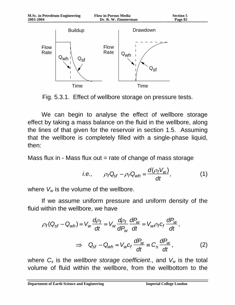
M.Sc. in Petroleum Engineering Flow in Porous Media Section 5 2003-2004 Dr. R. W. Zimmerman Page 82
Flow Rate
Time
Qwh Qsf
Buildup
Time
Flow Rate
Drawdown
Qsf
Qwh
Fig. 5.3.1. Effect of wellbore storage on pressure tests.
We can begin to analyse the effect of wellbore storage effect by taking a mass balance on the fluid in the wellbore, along the lines of that given for the reservoir in section 1.5. Assuming that the wellbore is completely filled with a single-phase liquid, then:
Mass flux in - Mass flux out = rate of change of mass storage
i.e., ρfQsf − ρfQwh =
d(ρfVw )dt
, (1)
where Vw is the volume of the wellbore.
If we assume uniform pressure and uniform density of the fluid within the wellbore, we have
ρf (Qsf − Qwh ) = Vw
dρfdt
= VwdρfdPw
dPwdt
= VwρfcfdPwdt
,
⇒ Qsf − Qwh = Vwcf
dPwdt
≡ CsdPwdt
, (2)
where Cs is the wellbore storage coefficient., and Vw is the total volume of fluid within the wellbore, from the wellbottom to the
Department of Earth Science and Engineering Imperial College London
M.Sc. in Petroleum Engineering Flow in Porous Media Section 5 2003-2004 Dr. R. W. Zimmerman Page 83
surface. [If the wellbore is not fully filled with liquid, the appropriate expression for Cs can be found in Advances in Well Test Analysis by Earlougher (SPE, 1977)].
At early times after the start of a constant-rate drawdown test, Qwh = Q (the nominal flowrate), but Qsf ≅ 0 , so eq. (2) takes the form
−Q = Cs
dPwdt
. (3)
Eq. (3) can be integrated, using the initial condition that Pw = Pi when t = 0:
−
QCs
dt0
t
∫ = dPwPi
Pw(t )
∫ ⇒ Pw = Pi −
QtCs
. (4)
Eq. (4) can be written in dimensionless form as follows:
(1) Rewrite eq. (4) in terms of the dimensionless pressure:
PDw =
2πkH(Pi − Pw)μQ
=2πkHQtμQCs
. (5)
(2) Express the RHS of eq. (5) in terms of tD:
PDw =
2πkHQμQCs
φμctRw2tDw
k≡
tDwCD
, (6)
where the dimensionless wellbore storage coefficient CD is defined by
CD =
Cs
2πHφctRw2
, (7)
Department of Earth Science and Engineering Imperial College London
M.Sc. in Petroleum Engineering Flow in Porous Media Section 5 2003-2004 Dr. R. W. Zimmerman Page 84
with ct being the total reservoir compressibility. Aside from the factor of 2, CD is the ratio of the storativity of the borehole to the storativity of the rock that had occupied the borehole before it was drilled. On a log-log plot, eq. (6) takes the form
lnPDw = ln tDw − lnCD , ⇒
d lnPDwd lntDw
= 1. (8)
→ A slope of unity occurring at early times on a log-log plot (dimensionless or not) of wellbore pressure vs. time is therefore an indicator of a pressure response that is dominated by wellbore-storage effects.
5.4. Effect of wellbore storage on pressure tests
The preceding analysis focused on fluid produced from wellbore storage, and neglected flow from the reservoir into the wellbore. In reality, fluid is supplied to the wellhead by wellbore storage at early times, but these effects gradually die out as the flow regime in the wellbore reaches a steady-state. An analysis that includes both contributions to the measured well-head flowrate Qwh, i.e., from the wellbore storage and from the reservoir, can be carried out by solving eq. (2.1.1), with the inner boundary condition, eq. (2.1.3), replaced by (see eq. (5.3.2)):
2πkHμ
R dPdR
⎛
⎝ ⎜ ⎜
⎞
⎠ ⎟ ⎟
Rw
= Qwh + CsdPdt
⎛
⎝ ⎜ ⎜
⎞
⎠ ⎟ ⎟
Rw
. (10)
This problem has been solved by Wattenbarger and Ramey (SPEJ, 1970) using finite differences, and by Agarwal et al. (SPEJ, 1970) using Laplace transforms. The analysis shows that there are three regimes of behaviour for a well in an infinite reservoir, with skin and wellbore storage:
Department of Earth Science and Engineering Imperial College London
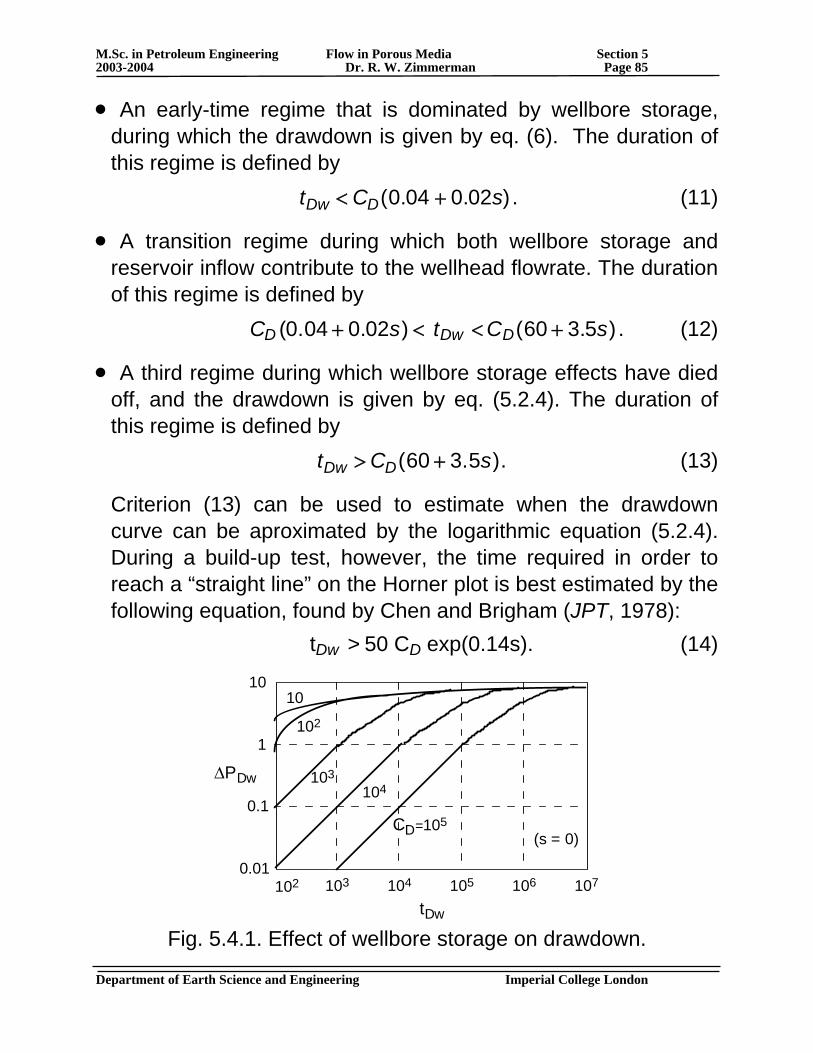
M.Sc. in Petroleum Engineering Flow in Porous Media Section 5 2003-2004 Dr. R. W. Zimmerman Page 85
• An early-time regime that is dominated by wellbore storage, during which the drawdown is given by eq. (6). The duration of this regime is defined by
tDw < CD(0.04 + 0.02s) . (11)
• A transition regime during which both wellbore storage and reservoir inflow contribute to the wellhead flowrate. The duration of this regime is defined by
CD (0.04 + 0.02s) < tDw < CD(60 + 3.5s) . (12)
• A third regime during which wellbore storage effects have died off, and the drawdown is given by eq. (5.2.4). The duration of this regime is defined by
tDw > CD(60 + 3.5s). (13)
Criterion (13) can be used to estimate when the drawdown curve can be aproximated by the logarithmic equation (5.2.4). During a build-up test, however, the time required in order to reach a “straight line” on the Horner plot is best estimated by the following equation, found by Chen and Brigham (JPT, 1978):
tDw > 50 CD exp(0.14s). (14)
tDw
ΔPDw
102 103 104 105 106 107
10
1
0.1
0.01
CD=105
104103
102
10
(s = 0)
Fig. 5.4.1. Effect of wellbore storage on drawdown.
Department of Earth Science and Engineering Imperial College London

Department of Earth Science and Engineering Imperial College London
M.Sc. in Petroleum Engineering Flow in Porous Media Section 6 2003-2004 Dr. R. W. Zimmerman Page 86
6. Outer Boundary Conditions
6.1. Well at the centre of a circular reservoir with constant pressure on its outer boundary and constant wellbore pressure Thus far, we have assumed that our wells are located in an infinite (or at least semi-infinite) reservoir. In reality, the reservoir is always of finite size, and the pressure disturbance will eventually reach some outer boundary that effectively encloses the reservoir. This outer boundary may be an “aquifer”, i.e., a vast expanse of water-filled rock that surrounds the hydrocarbon-filled “reservoir”. In this case, the appropriate outer boundary condition may be one of constant pressure.
On the other hand, if a number of wells are producing from the same reservoir, each will drain fluid from only a finite region, and so each well will effectively behave as if it were surrounded by a no-flow boundary, as illustrated in Fig. 6.1.1. (The effective drainage area of each well will depend on the production rate of that well, and of all nearby wells.)
WellsOuter boundary of reservoir
No-flow boundaries
Fig. 6.1.1. Reservoir with several production wells.
Department of Earth Science and Engineering Imperial College London
M.Sc. in Petroleum Engineering Flow in Porous Media Section 6 2003-2004 Dr. R. W. Zimmerman Page 87
Problems involving wells producing from a finite, bounded drainage area can be solved using either of two mathematical techniques: Laplace transforms, or the method of eigenfunction expansions. Laplace transforms will be discussed in section 7. In this section we use the method of eigenfunction expansions to solve the problem of a well located at the centre of a circular reservoir, with its outer boundary maintained at constant pressure, and with a constant borehole pressure. This is by no means the most important of such problems, but it will allow us to develop the method of eigenfunction expansions in a (relatively) simple context.
The first point to note is that the Boltzmann transformation is of no use in bounded-reservoir problems. The reason that it “worked” in the infinite-reservoir case is that the initial condition, at t = 0, and the outer boundary condition, at R → ∞ , both correspond to the same limit η → ∞ , and both also correspond to the initial pressure, Pi. This “collapsing” of two conditions into one equivalent condition allowed us to replace a 2nd-order PDE (which requires 2 BCs + 1 IC = 3 conditions) with a 2nd-order ODE (which requires a total of 2 subsidiary conditions).
This does not occur in the bounded-reservoir problem, because the outer BC is imposed at R = Re, and R = Re does not correspond to a fixed value of the Boltzmann variable, η. (In general, a Boltzmann-type transformation will not work in a problem that contains a natural length scale, such as a wellbore radius or an outer radius; the problem of an infinitely-small line-source in an infinite reservoir had no natural length scale associated with it.)
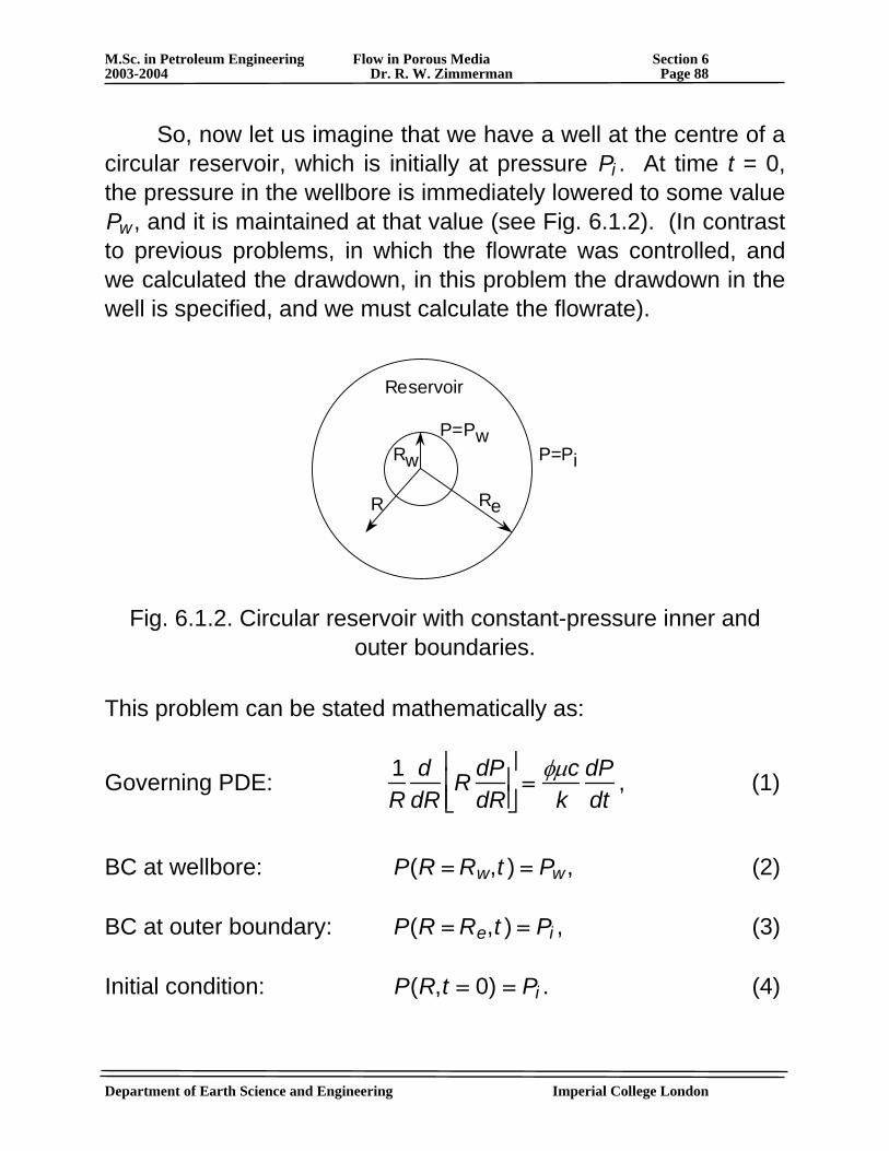
Department of Earth Science and Engineering Imperial College London
M.Sc. in Petroleum Engineering Flow in Porous Media Section 6 2003-2004 Dr. R. W. Zimmerman Page 88
So, now let us imagine that we have a well at the centre of a circular reservoir, which is initially at pressure Pi . At time t = 0, the pressure in the wellbore is immediately lowered to some value Pw, and it is maintained at that value (see Fig. 6.1.2). (In contrast to previous problems, in which the flowrate was controlled, and we calculated the drawdown, in this problem the drawdown in the well is specified, and we must calculate the flowrate).
Rw
Re
Reservoir
P=Pi
R
P=Pw
Fig. 6.1.2. Circular reservoir with constant-pressure inner and outer boundaries.
This problem can be stated mathematically as:
Governing PDE:
1R
ddR
R dPdR
⎡
⎣ ⎢ ⎢
⎤
⎦ ⎥ ⎥
=φμc
kdPdt
, (1)
BC at wellbore: P(R = Rw,t ) = Pw , (2)
BC at outer boundary: P(R = Re,t ) = Pi , (3)
Initial condition: P(R,t = 0) = Pi . (4)
Department of Earth Science and Engineering Imperial College London
M.Sc. in Petroleum Engineering Flow in Porous Media Section 6 2003-2004 Dr. R. W. Zimmerman Page 89
The first step in solving this problem is to simplify its appearance by introducing dimensionless variables. Define
Dimensionless radius: RD = R /Rw , (5)
Dimensionless time: tD =
ktφμcRw
2, (6)
Dimensionless drawdown: PD =
Pi − PPi − Pw
. (7)
(Note that the production rate Q is unknown a priori, so we can’t define PD as we did before, in terms of Q.)
In terms of these variables, eqs. (1-4) take the form
Governing PDE:
1RD
ddRD
RDdPDdRD
⎡
⎣ ⎢ ⎢
⎤
⎦ ⎥ ⎥
=dPDdtD
, (8)
BC at wellbore: PD(RD = Rw / Rw = 1,tD ) = 1, (9)
BC at outer boundary: PD(RD = Re / Rw ≡ RDe,tD ) = 0 , (10)
Initial condition: PD(RD,tD = 0) = 0 . (11)
We next invoke the principle of superposition to break up the pressure into a steady-state part, PD
s (RD ), and a transient part, pD(RD,tD ) :
PD(RD,tD) = PDs(RD ) + pD(RD,tD ) . (12)
Department of Earth Science and Engineering Imperial College London
M.Sc. in Petroleum Engineering Flow in Porous Media Section 6 2003-2004 Dr. R. W. Zimmerman Page 90
By definition, the steady-state pressure function must satisfy eq. (8), as well as both BCs, (9) and (10). The time derivative is zero for the steady-state part, so the actual governing differential equation for PD
s (RD ) is eq. (8) with the RHS set to zero. Therefore, PD
s (RD ) is governed by
Governing ODE:
1RD
ddRD
RDdPD
s
dRD
⎛
⎝ ⎜ ⎜
⎞
⎠ ⎟ ⎟ = 0 , (13)
BC at wellbore: 1)1( ==Ds
D RP , (14)
BC at outer boundary: PDs (RD = RDe ) = 0. (15)
♦ Integrate eq. (13) once to get (i.e., an indefinite integral):
RD
dPDs
dRD= B = constant . (16)
♦ Separate the variables in eq. (16) and integrate again:
dPD
sPD
s (RD )
∫ = B dRDRD
RD
∫ + A,
⇒ PDs(RD ) = B lnRD + A. (17)
♦ Comparison of eq. (17) with eqs. (14) and (15) shows that A = 1 and B = −1/ lnRDe , so eq. (17) can be written as
⇒ PD
s(RD ) = 1−lnRDlnRDe
=− ln(RD / RDe )
lnRDe. (18)
Department of Earth Science and Engineering Imperial College London
M.Sc. in Petroleum Engineering Flow in Porous Media Section 6 2003-2004 Dr. R. W. Zimmerman Page 91
Note 1: The steady-state solution satisfies the diffusion equation (8), and the boundary conditions (9,10), but it doesn’t satisfy the initial condition (11); this is why we also need the transient component of the solution.
Note 2: Eq. (18) is just the Thiem equation, eq. (1.4.3), in a dimensionless form.
If we substitute (12) into eqs. (8-11), and make use of eq. (18), we see that the transient pressure function must satisfy
Governing PDE:
1RD
ddRD
RDdpDdRD
⎡
⎣ ⎢ ⎢
⎤
⎦ ⎥ ⎥
=dpDdtD
, (19)
BC at wellbore: pD(RD = 1,tD ) = 0 , (20)
BC at outer boundary: pD(RD = RDe,tD) = 0, (21)
Initial condition: pD(RD,t = 0) =
ln(RD /RDe )lnRDe
. (22)
Thus far, we have transformed a diffusion equation with a nonzero BC, eq. (9), and zero IC, eq. (11), into a diffusion equation with zero BC and a nonzero IC, eq. (22). We may not appear to be making progress, but we are, because the eigenfunction method requires “zero” boundary conditions, but does not require “zero” initial conditions.
To solve eqs. (19-22), we again make use of the superposition principle, and first search for (as many functions as we can find!) that each satisfy eq. (19) and the boundary conditions (20,21); later, we will superpose these functions to satisfy eq. (22).
Department of Earth Science and Engineering Imperial College London
M.Sc. in Petroleum Engineering Flow in Porous Media Section 6 2003-2004 Dr. R. W. Zimmerman Page 92
(a) Assume that these functions can be written in the form
pD(RD,tD ) = F(RD )G(tD) . (23)
(b) Insert eq. (23) into eq. (19) to find:
DD
DD
DDD dt
dGRFdRdFR
dRd
RtG )(1)( =⎥
⎦
⎤⎢⎣
⎡⎟⎟⎠
⎞⎜⎜⎝
⎛. (24)
(c) Divide through by F(RD )G(tD ) to find:
DDDD
DDD dtdG
tGdRdFR
dRd
RFR )(1
)(1
=⎟⎟⎠
⎞⎜⎜⎝
⎛. (25)
(d) The LHS of eq. (25) doesn’t depend on tD, and the RHS doesn’t depend on RD; since they are equal to each other, they cannot depend on either variable! Hence, each side of eq. (25) must equal a constant, which we call −λ2:
2
)(1
)(1 λ−==⎟⎟
⎠
⎞⎜⎜⎝
⎛
DDDD
DDD dtdG
tGdRdFR
dRd
RFR . (26)
(e) The space-dependent part of eq. (26) can be written as
′ ′ F (RD) +
1RD
′ F (RD) + λ2F(RD ) = 0 . (27)
We now make a change of variables x = λRD , after which eq. (27) can be written as
′ ′ F (x ) +
1x
′ F (x) + F(x) = 0. (28)
Department of Earth Science and Engineering Imperial College London
M.Sc. in Petroleum Engineering Flow in Porous Media Section 6 2003-2004 Dr. R. W. Zimmerman Page 93
Eq. (28) is known as a Bessel equation of order zero. It is a 2nd-order ordinary differential equation, so it must have two independent solutions. One solution is readily found by assuming a power-series solution:
F(x) = an
n=0
∞∑ xn. (29)
♦ If we insert eq. (29) into eq. (28), we find
0)1(0
2
0
2
0
=++− ∑∑∑∞
=
−∞
=
−∞
=
n
nn
n
nn
n
nn xaxnaxann . (30)
♦ In order to have x appear to the nth power in each term, we let n → n + 2 in the first two series, which, after combining the first two series and taking the “unmatched” terms outside of the series, leads to
0])2[(00
221
12
0 =++++ ∑∞
=+
−− n
nnn xaanxaxa . (31)
♦ The coefficient of each power of x in eq. (31) must be zero. The x−2 term already has a factor of zero, so it will vanish regardless of the choice of a0; we may as well pick
a0 = 1. (32)
♦ In order for the x−1 term to vanish, we must pick
a1 = 0. (33)
♦ For all higher-order terms to vanish, eq. (31) shows that the coefficients must satisfy the following recursion relationship:
an+2 =
−an
(n + 2)2. (34)
Department of Earth Science and Engineering Imperial College London
M.Sc. in Petroleum Engineering Flow in Porous Media Section 6 2003-2004 Dr. R. W. Zimmerman Page 94
♦ This recursion relationship allows us to generate all subsequent coefficients, starting with the first two coefficients, given by eqs. (32) and (33):
a3 = a5 = a7 = ... = 0 , (35)
a2 =
−14
, a4 =1
64, a6 =
−12304
.... (36)
The solution to eq. (28) that is given by eqs. (29), (35) and (36) is known as the Bessel function of the first kind (of order zero), and is denoted by Jo(x):
...2304644
1)(642
0 +−+−=xxxxJ ,
or ...)!3(2)!2(2)!1(2
1)( 26
6
24
4
22
2
0 +−+−=xxxxJ , (37)
where n! ≡ 1× 2 × 3 × ... × n is the factorial function.
The function J0(x) is similar to a damped cosine function (see Fig. 6.1.3). It “starts” at J0(0) = 1, oscillates (but not quite periodically), and then slowly decays to zero according to (see Theory of Bessel Functions, G. N. Watson, 1922, or any book on advanced applied mathematics)
∞→⎟⎠⎞
⎜⎝⎛ −≈ xas
4cos2)(0
ππ
xx
xJ . (38)
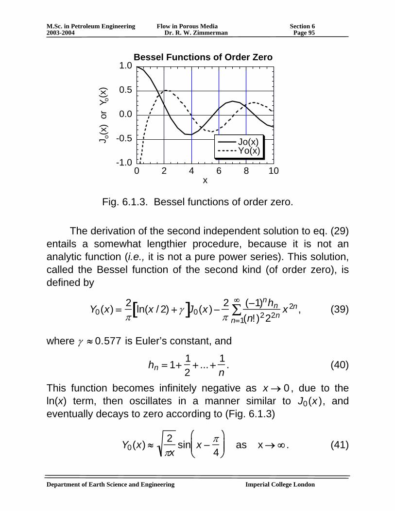
Department of Earth Science and Engineering Imperial College London
M.Sc. in Petroleum Engineering Flow in Porous Media Section 6 2003-2004 Dr. R. W. Zimmerman Page 95
-1.0
-0.5
0.0
0.5
1.0
0 2 4 6 8 10
Bessel Functions of Order Zero
Jo(x)Yo(x)
J o(x
) or
Yo(
x)
x
Fig. 6.1.3. Bessel functions of order zero.
The derivation of the second independent solution to eq. (29) entails a somewhat lengthier procedure, because it is not an analytic function (i.e., it is not a pure power series). This solution, called the Bessel function of the second kind (of order zero), is defined by
Y0(x) =
2π
ln(x / 2) + γ[ ]J0(x ) −2π
(−1)nhn
(n! )222nn=1
∞∑ x 2n, (39)
where γ ≈ 0.577 is Euler’s constant, and
hn = 1+
12
+ ... +1n
. (40)
This function becomes infinitely negative as x → 0 , due to the ln(x) term, then oscillates in a manner similar to J0(x ), and eventually decays to zero according to (Fig. 6.1.3)
Y0(x) ≈
2πx
sin x −π4
⎛
⎝ ⎜ ⎜
⎞
⎠ ⎟ ⎟ as x → ∞ . (41)
Department of Earth Science and Engineering Imperial College London
M.Sc. in Petroleum Engineering Flow in Porous Media Section 6 2003-2004 Dr. R. W. Zimmerman Page 96
The general solution to eq. (28) can be written as a linear combination of these two kinds of Bessel functions:
F(x) = AJ0(x) + BY0(x) . (42)
Recalling that x = λRD , we have
F(RD ) = AJ0(λRD ) + BY0(λRD) . (43)
Eq. (43) will be a solution to eq. (28) for any value of λ. However, it will satisfy the boundary conditions (20) and (21) only for certain special values of λ, which we will now find. Insertion of eq. (43) into BCs (20) and (21) yields
AJ0(λ) + BY0(λ) = 0 , (44)
AJ0(λRDe ) + BY0(λRDe ) = 0 . (45)
These two equations can be written in matrix form as
J0(λ) Y0(λ)J0(λRDe ) Y0(λRDe )
⎡
⎣ ⎢ ⎢
⎤
⎦ ⎥ ⎥
AB
⎡
⎣ ⎢ ⎢
⎤
⎦ ⎥ ⎥
=00
⎡
⎣ ⎢ ⎢
⎤
⎦ ⎥ ⎥ . (46)
In order for eq. (46) to have non-zero solutions for A and B, the determinant of the matrix must be zero:
J0(λ)Y0(λRDe ) − Y0(λ)J0(λRDe ) = 0. (47)
The values of λ that satisfy eq. (47) are the eigenvalues of this problem. They will depend on the dimensionless size of the reservoir, RDe = RD / Rw . There will always be an infinite number of eigenvalues, and they can be arranged in order as
Department of Earth Science and Engineering Imperial College London
M.Sc. in Petroleum Engineering Flow in Porous Media Section 6 2003-2004 Dr. R. W. Zimmerman Page 97
. (48)
Each of these eigenvalues is associated with its own eigenfunction (see eq. (43)):
Fn(RD ) = AnJ0(λnRD) + BnY0(λnRD) . (49)
From eq. (44), the constants An and Bn are related by
)()(
0
0
n
nnn Y
JABλ
λ−= , (50)
and so eq. (49) can be written as
Fn(RD ) = AnJ0(λnRD) − An
J0(λn )Y0(λn)
Y0(λnRD)
=
AnY0(λn)
Y0(λn)J0(λnRD ) − J0(λn)Y0(λnRD )[ ]
= Cn Y0(λn)J0(λnRD ) − J0(λn)Y0(λnRD)[ ], (51)
where the Cn are arbitrary constants, and the functions inside the brackets are the eigenfunctions of this problem.
We now return to the time-dependent part of the solution, which, according to eq. (26), must satisfy
dGndtD
= −λn2Gn(tD ) . (52)
The solution to eq. (52) is
Gn(tD) = e −λn2tD . (53)
Department of Earth Science and Engineering Imperial College London
M.Sc. in Petroleum Engineering Flow in Porous Media Section 6 2003-2004 Dr. R. W. Zimmerman Page 98
Recalling eq. (23), the most general solution that satisfies the diffusion equation (19) and the BCs (20,21) is given by
pD(RD,tD ) = Cn Y0(λn)J0(λnRD ) − J0(λn)Y0(λnRD)[ ]
n=1
∞∑ e −λn
2tD . (54)
All that remains now is to satisfy the initial condition, eq. (22). Evaluating eq. (54) at tD = 0, and invoking eq. (22), yields
Cn Y0(λn )J0(λnRD ) − J0(λn )Y0(λnRD )[ ]n=1
∞∑ =
ln(RD / RDe )lnRDe
. (55)
The constants Cn must be chosen so as to satisfy eq. (55) for all values of the dimensionless radius. This can be done using the orthogonality properties of eigenfunctions (see Muskat, The Flow of Homogeneous Fluids through Porous Media, 1937, chapter 10 for details). The result is
Cn =
πJ0(λn )J0(λnRDe )J0
2(λn) − J02(λnRDe )
. (56)
We now combine the transient and steady-state pressures to find, from eqs. (12), (24), (54) and (56), the complete solution to this problem:
Dnt
nDnn
Denn
Denn
De
DeDDDD eRU
RJJRJJ
RRRtRP
2
120
20
00 )()()()()(
ln)/ln(),( λλ
λλλλπ −
∞
=∑ −
+−
= (57)
where Un(λnRD ) = Y0(λn)J0(λnRD ) − J0(λn)Y0(λnRD ) .
This completes the solution to this problem. The dimensional values can be found by recalling eqs. (5-7).
The flowrate into the well can be found by differentiating the pressure, and applying Darcy’s law at the wellbore. A detailed
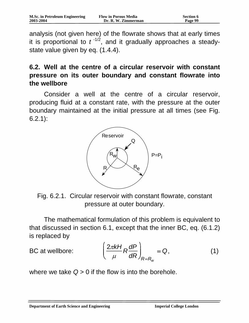
Department of Earth Science and Engineering Imperial College London
M.Sc. in Petroleum Engineering Flow in Porous Media Section 6 2003-2004 Dr. R. W. Zimmerman Page 99
analysis (not given here) of the flowrate shows that at early times it is proportional to t -1/2, and it gradually approaches a steady-state value given by eq. (1.4.4).
6.2. Well at the centre of a circular reservoir with constant pressure on its outer boundary and constant flowrate into the wellbore Consider a well at the centre of a circular reservoir, producing fluid at a constant rate, with the pressure at the outer boundary maintained at the initial pressure at all times (see Fig. 6.2.1):
Rw
Re
Reservoir
P=Pi
R
Q
Fig. 6.2.1. Circular reservoir with constant flowrate, constant
pressure at outer boundary.
The mathematical formulation of this problem is equivalent to that discussed in section 6.1, except that the inner BC, eq. (6.1.2) is replaced by
BC at wellbore:
2πkHμ
R dPdR
⎛
⎝ ⎜ ⎜
⎞
⎠ ⎟ ⎟
R=Rw
= Q , (1)
where we take Q > 0 if the flow is into the borehole.
Department of Earth Science and Engineering Imperial College London
M.Sc. in Petroleum Engineering Flow in Porous Media Section 6 2003-2004 Dr. R. W. Zimmerman Page 100
This problem can also be solved using the method of eigenfunction expansions, as in the previous section. The solution is (Muskat, Flow of Homogeneous Fluids through Porous Media, 1937, p. 643):
ΔPD(RD,tD) = − ln RD
RDe
⎛
⎝ ⎜ ⎜
⎞
⎠ ⎟ ⎟ −
π J02(λnRDe )Un(λnRD)
λn [J02(λnRDe ) − J1
2(λn)]n=1
∞∑ e−λn
2tD , (2)
where the eigenfunctions Un are given by
Un(λnRD ) = Y1(λn)J0(λnRD ) − J1(λn)Y0(λnRD ) , (3)
and the eigenvalues λn are defined implicitly by
Un(λnRDe ) = Y1(λn)J0(λnRDe ) − J1(λn)Y0(λnRDe ) = 0. (4)
The functions J1 and Y1 are Bessel functions of order one, and are defined by
J1(x) ≡ −
dJ0(x )dx
, Y1(x ) ≡ −dY0(x)
dx. (5)
The dimensionless variables in eq. (2) are defined by
Dimensionless radius: RD = R /Rw , (6)
Dimensionless time: tD =
ktφμcRw
2, (7)
Dimensionless pressure: ΔPD =
2πkH(Pi − P)μQ
. (8)
The pressure in the wellbore, ΔPDw(tD), is found by setting RD = 1 in eq. (2), and then making use of the following Bessel-function identity (see Muskat, p. 631):
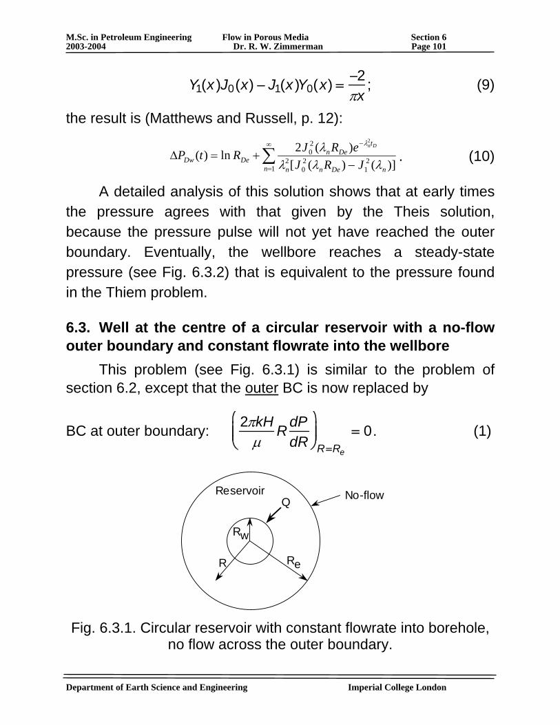
Department of Earth Science and Engineering Imperial College London
M.Sc. in Petroleum Engineering Flow in Porous Media Section 6 2003-2004 Dr. R. W. Zimmerman Page 101
Y1(x )J0(x) − J1(x )Y0(x) =
−2πx
; (9)
the result is (Matthews and Russell, p. 12):
∑∞
=
−
−+=Δ
12
120
2
20
)]()([)(2ln)(
2
n nDenn
tDen
DeDw JRJeRJRtP
Dn
λλλλ λ
. (10)
A detailed analysis of this solution shows that at early times the pressure agrees with that given by the Theis solution, because the pressure pulse will not yet have reached the outer boundary. Eventually, the wellbore reaches a steady-state pressure (see Fig. 6.3.2) that is equivalent to the pressure found in the Thiem problem.
6.3. Well at the centre of a circular reservoir with a no-flow outer boundary and constant flowrate into the wellbore This problem (see Fig. 6.3.1) is similar to the problem of section 6.2, except that the outer BC is now replaced by
BC at outer boundary:
2πkHμ
R dPdR
⎛
⎝ ⎜ ⎜
⎞
⎠ ⎟ ⎟
R=Re
= 0. (1)
Rw
Re
Reservoir No-flow
R
Q
Fig. 6.3.1. Circular reservoir with constant flowrate into borehole,
no flow across the outer boundary.
Department of Earth Science and Engineering Imperial College London
M.Sc. in Petroleum Engineering Flow in Porous Media Section 6 2003-2004 Dr. R. W. Zimmerman Page 102
The solution to this problem was found by Muskat in 1937 using the eigenfunction method; it was re-derived by van Everdingen and Hurst in 1949 (Trans. AIME, 1949), using Laplace transforms (see section 7). The solution is
⎥⎦
⎤⎢⎣
⎡−+
−=Δ DDeD
D
DeDDD RRtR
RtRP ln
412),( 2
2
2
⎥⎦
⎤⎢⎣
⎡
−−−−
− 22
244
)1(412ln43
De
DeDeDeDe
RRRRR
Dnt
n nDenn
DnnDen eJRJ
RURJ 2
12
12
1
21
)]()([)()( λ
λλλλλπ −
∞
=∑ −
+ , (2)
where the eigenfunctions Un are given by
)()()()()( 0101 DnnDnnDnn RJYRYJRU λλλλλ −= , (3)
the eigenvalues λn are defined implicitly by
0)()()()( 1111 =− DennDenn RJYRYJ λλλλ , (4)
and the dimensionless variables are defined as in section 6.2. Because of the importance of this problem, we will examine the solution in detail. The pressure in the wellbore is found by setting RD = 1 in eq. (2), and again using eq. (6.2.9) to simplify:
ΔPDw (tD ) =
1RDe
2 − 112
+ 2tD⎡
⎣ ⎢ ⎢
⎤
⎦ ⎥ ⎥
−3RDe
4 − 4RDe4 lnRDe − 2RDe
2 − 14(RDe
2 − 1)2⎡
⎣ ⎢ ⎢
⎤
⎦ ⎥ ⎥
∑∞
=
−
−+
12
12
12
21
)]()([)(2
2
n nDenn
tDen
JRJeRJ Dn
λλλλ λ
. (5)
Department of Earth Science and Engineering Imperial College London
M.Sc. in Petroleum Engineering Flow in Porous Media Section 6 2003-2004 Dr. R. W. Zimmerman Page 103
In most cases of practical interest, however, 1>>DeR , and eq. (5) can effectively be written as
ΔPDw (tD ) =
2tDRDe
2+ lnRDe −
34
+
2J12(λnRDe )e−λn
2tD
λn2[J1
2(λnRDe ) − J12(λn)]n=1
∞∑ . (6)
There are three important time regimes in this problem:
(i) A regime in which t is sufficiently large that the logarithmic approximation to the line-source solution is valid, but for which the leading edge of the pressure pulse has not yet reached the outer boundary of the reservoir. From eq. (2.4.7) and Fig. 2.5.1, we find that this regime is defined by:
25 < tDw < 0.1RDe2 . (7)
• It is not easy to see that eq. (5) reduces to eq. (2.4.10) during this time regime, but it does.
(ii) A second regime that is “late” enough that the presence of the closed outer boundary is felt at the well, but still early enough that the exponential terms in eq. (6) have not yet died out. The start of this regime is given by the upper bound in eq. (7); it ends when tDw ≈ 0.3RDe
2 (see Tutorial Sheet 5). This regime is therefore defined by
0.1RDe2 < tDw < 0.3RDe
2 . (8)
In this regime we must use the entire series in eq. (6) to calculate the wellbore pressure, and the ΔPw(tDw) curve has no simple description.
(iii) A third regime that is late enough such that the exponential terms in eq. (6) have died out. This regime is defined by
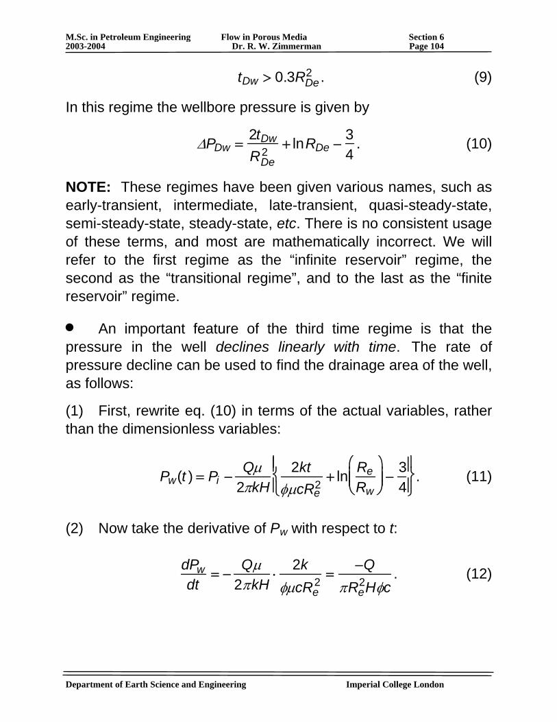
Department of Earth Science and Engineering Imperial College London
M.Sc. in Petroleum Engineering Flow in Porous Media Section 6 2003-2004 Dr. R. W. Zimmerman Page 104
tDw > 0.3RDe2 . (9)
In this regime the wellbore pressure is given by
ΔPDw =
2tDw
RDe2
+ lnRDe −34
. (10)
NOTE: These regimes have been given various names, such as early-transient, intermediate, late-transient, quasi-steady-state, semi-steady-state, steady-state, etc. There is no consistent usage of these terms, and most are mathematically incorrect. We will refer to the first regime as the “infinite reservoir” regime, the second as the “transitional regime”, and to the last as the “finite reservoir” regime.
• An important feature of the third time regime is that the pressure in the well declines linearly with time. The rate of pressure decline can be used to find the drainage area of the well, as follows:
(1) First, rewrite eq. (10) in terms of the actual variables, rather than the dimensionless variables:
Pw(t ) = Pi −
Qμ2πkH
2ktφμcRe
2 + ln ReRw
⎛
⎝ ⎜ ⎜
⎞
⎠ ⎟ ⎟ −
34
⎧ ⎨ ⎪
⎩ ⎪
⎫ ⎬ ⎪
⎭ ⎪ . (11)
(2) Now take the derivative of Pw with respect to t:
dPwdt
= −Qμ
2πkH⋅
2kφμcRe
2=
−QπRe
2Hφc. (12)
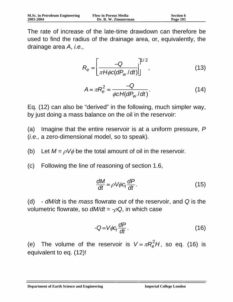
Department of Earth Science and Engineering Imperial College London
M.Sc. in Petroleum Engineering Flow in Porous Media Section 6 2003-2004 Dr. R. W. Zimmerman Page 105
The rate of increase of the late-time drawdown can therefore be used to find the radius of the drainage area, or, equivalently, the drainage area A, i.e.,
Re =
−QπHφc(dPw /dt )
⎡
⎣ ⎢ ⎢
⎤
⎦ ⎥ ⎥
1/ 2
, (13)
A = πRe
2 =−Q
φcH(dPw /dt ). (14)
Eq. (12) can also be “derived” in the following, much simpler way, by just doing a mass balance on the oil in the reservoir:
(a) Imagine that the entire reservoir is at a uniform pressure, P (i.e., a zero-dimensional model, so to speak).
(b) Let M = ρVφ be the total amount of oil in the reservoir.
(c) Following the line of reasoning of section 1.6,
dMdt = ρVφct
dPdt . (15)
(d) - dM/dt is the mass flowrate out of the reservoir, and Q is the volumetric flowrate, so dM/dt = -ρQ, in which case
-Q =Vφct
dPdt . (16)
(e) The volume of the reservoir is V = πRe2H , so eq. (16) is
equivalent to eq. (12)!
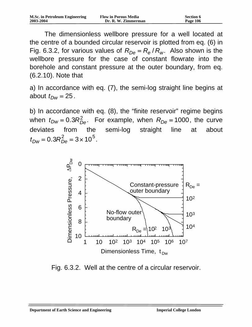
Department of Earth Science and Engineering Imperial College London
M.Sc. in Petroleum Engineering Flow in Porous Media Section 6 2003-2004 Dr. R. W. Zimmerman Page 106
The dimensionless wellbore pressure for a well located at the centre of a bounded circular reservoir is plotted from eq. (6) in Fig. 6.3.2, for various values of RDe = Re / Rw . Also shown is the wellbore pressure for the case of constant flowrate into the borehole and constant pressure at the outer boundary, from eq. (6.2.10). Note that
a) In accordance with eq. (7), the semi-log straight line begins at about tDw = 25 .
b) In accordance with eq. (8), the “finite reservoir” regime begins when tDw = 0.3RDe
2 . For example, when RDe = 1000, the curve deviates from the semi-log straight line at about
tDw = 0.3RDe2 = 3 × 10⁵.
0
2
4
6
8
101 10 102 103 104 105 106 107D
imen
sion
less
Pre
ssur
e,
ΔP D
w
Dimensionless Time, t Dw
RDe = 102 103
No-flow outer boundary
Constant-pressure outer boundary
102
103
RDe =
104
Fig. 6.3.2. Well at the centre of a circular reservoir.
Department of Earth Science and Engineering Imperial College London
M.Sc. in Petroleum Engineering Flow in Porous Media Section 6 2003-2004 Dr. R. W. Zimmerman Page 107
6.4. Non-Circular Drainage Regions If the drainage region is not circular, and/or the well is not located at the centre, then the problem treated in section 6.3 is more difficult to solve. If the drainage region is bounded by a polygon (as would occur if the reservoir was bounded by a set of linear faults), then the problem can be solved by superposing solutions from appropriately located image wells, as in section 4.3. For example, an infinite array of image wells arranged on a square lattice will create a square reservoir that is bounded by four no-flow boundaries, etc. Some examples of this type of analysis can be found in Well Testing in Heterogeneous Formations, by T. D. Streltsova, Wiley, 1988. Without going into the details of this analysis, the following can be said about a well producing from within a non-circular drainage region: • There is an “infinite reservoir” regime, during which the pressure pulse has not yet reached any portion of the outer boundary. The duration of this regime can be calculated using eq. (1.6.11), if the geometry of the drainage area and the location of the well is known. During this regime,
ΔPDw =
12
[ln(tDw ) + 0.80907]. (1)
At sufficiently long times, the mass-balance argument presented in the previous section must hold, and so the rate at which the wellbore drawdown changes must be given by eq. (6.3.12), with Re
2 replaced by A / π . Hence, an equation of the same form as eq. (6.3.10) must hold for the drawdown, except that the constant term may be different.
The duration of this regime is roughly given by eq. (6.3.9), again with Re
2 replaced by A / π , although the start of this regime
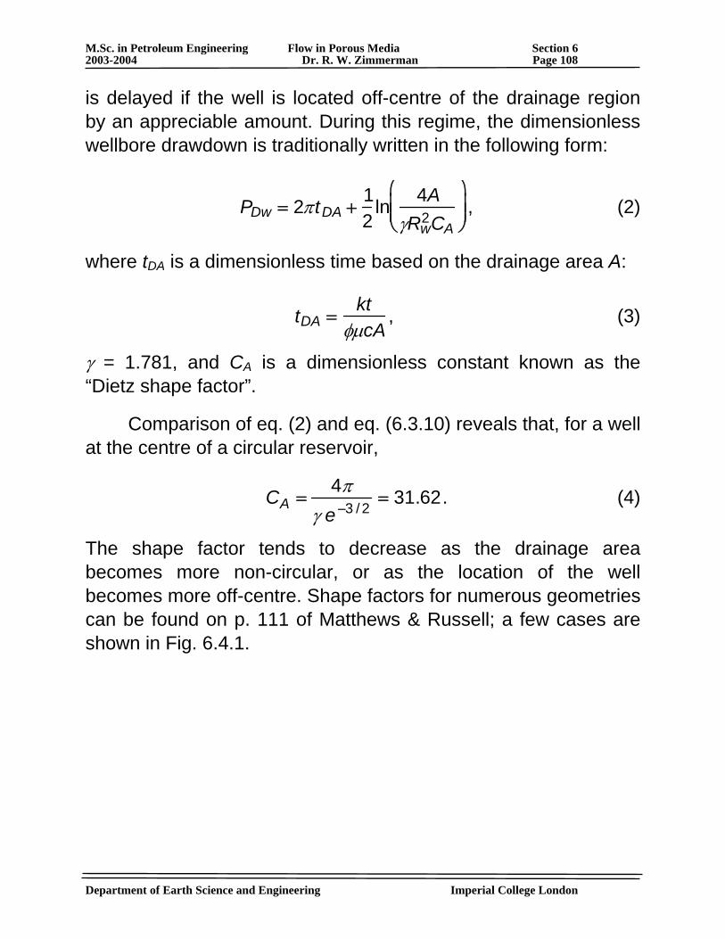
Department of Earth Science and Engineering Imperial College London
M.Sc. in Petroleum Engineering Flow in Porous Media Section 6 2003-2004 Dr. R. W. Zimmerman Page 108
is delayed if the well is located off-centre of the drainage region by an appreciable amount. During this regime, the dimensionless wellbore drawdown is traditionally written in the following form:
PDw = 2πtDA +
12
ln 4AγRw
2CA
⎛
⎝ ⎜ ⎜
⎞
⎠ ⎟ ⎟ , (2)
where tDA is a dimensionless time based on the drainage area A:
tDA =
ktφμcA
, (3)
γ = 1.781, and CA is a dimensionless constant known as the “Dietz shape factor”.
Comparison of eq. (2) and eq. (6.3.10) reveals that, for a well at the centre of a circular reservoir,
CA =
4πγ e −3 /2 = 31.62. (4)
The shape factor tends to decrease as the drainage area becomes more non-circular, or as the location of the well becomes more off-centre. Shape factors for numerous geometries can be found on p. 111 of Matthews & Russell; a few cases are shown in Fig. 6.4.1.
Department of Earth Science and Engineering Imperial College London
M.Sc. in Petroleum Engineering Flow in Porous Media Section 6 2003-2004 Dr. R. W. Zimmerman Page 109
31.6
CA
31.6
27.6
12.9
1
1
1
1
2
2
4
4
CA
22.6
2.07
2.36
0.232
Fig. 6.4.1. Dietz shape factors for various geometries. ______________________________________________ Tutorial Sheet 5: (1) Show that the transition regime for the closed circular reservoir problem ends when tDw = 0.3RDe
2 . Hints: (a) e−x ≈ 0 when x > 4, so the terms in the series will be negligible when λn
2tDw > 4 for all n. (b) When RDe is large, the smallest eigenvalue, λ1, i.e., the smallest value of λ that satisfies eq. (6.3.4), is very small. This fact should help to estimate the value of λ1 as a function of RDe . Also, make use of eqs. (6.2.37,39,48), and Fig. 6.1.3.
(2) Starting with eq. (6.3.2), calculate the average pressure in the reservoir during the finite reservoir regime ( tDw > 0.3RDe
2 ), as a function of time. Is your result consistent with the mass-balance that is embodied in eq. (6.3.15)?
M.Sc. in Petroleum Engineering Flow in Porous Media Section 7 2003-2004 Dr. R. W. Zimmerman Page 110 7. Laplace Transform Methods The diffusion equation for fluid flow in a porous medium, in the linearised form that is often used, is a linear PDE. As such, many of the classical methods of applied mathematics can be used to solve it. In section 2.1 we used the Boltzmann transformation to solve the problem of a single, fully-penetrating well in an infinite, homogeneous reservoir, although we saw in section 6.1 that this method is only occasionally applicable. In section 6 we used the method of eigenfunction expansions to solve problems involving a well in a circular reservoir. Although this method is in general the most widely-used method in applied mathematics, it has not been used very often in petroleum engineering. Traditionally, reservoir engineers have solved the diffusion equation using the method of Laplace transforms. In this section we will describe the Laplace transform approach, and give an example of its use in solving reservoir problems.
7.1. Laplace transforms The method of Laplace transforms allows us to transform PDEs, which are generally difficult to solve, into ODEs, which can be solved in essentially all cases. Specifically, the function P(R,t), which satisfies the PDE, is transformed into a different function
s)(R,P~ , which satisfies an ODE. This ODE is then solved to yield s)(R,P~ . The only difficult part of the method of Laplace transforms
is the process of “inverting” the function from the “Laplace domain” back into the “time domain”, to get P(R,t). This last step can be achieved either by contour integration in the complex plane, or by numerical integration along the real axis. In this section we present the definition of the Laplace transform, along with a few of its more important properties. A fuller treatment can be found in essentially any textbook on Department of Earth Science and Engineering Imperial College London
M.Sc. in Petroleum Engineering Flow in Porous Media Section 7 2003-2004 Dr. R. W. Zimmerman Page 111 advanced applied mathematics. Three books that are devoted exclusively to Laplace (and related) transforms are
(1) Operational Mathematics, R. V. Churchill, McGraw-Hill, New York, 1958.
(2) Operational Methods in Applied Mathematics, H. S. Carslaw and J. C. Jaeger, Oxford University Press, Oxford, 1949.
(3) Integral Transforms in Mathematical Physics, C. J. Tranter, Chapman & Hall, London, 1971.
Definition: If we have a function f (t) , its Laplace transform is defined by
∫∞
−≡≡0
dtstetfsftfL )()()}({ ~ . (1)
Both notations, L{ f (t) } and )(sf~ , are useful, depending on the context. In the general theory of Laplace transforms, s must be regarded as a complex variable, but for our purposes this is usually not necessary. If we have a function of two variables, such as P(R,t), we can defined its Laplace transform in the same manner:
∫≡∞
−
0)()( tdetR,PsR,P st~ . (2)
Note that the Laplace transform is taken with respect to the time variable, not the spatial variable. To simplify the notation, we will usually suppress the R variable when discussing the general theory.
Department of Earth Science and Engineering Imperial College London
M.Sc. in Petroleum Engineering Flow in Porous Media Section 7 2003-2004 Dr. R. W. Zimmerman Page 112 The Laplace transform operator L is a linear operator, because it follows directly from definition (1) that
L{cf(t)} = cf (t)e−stdt
0
∞∫ = c f(t)e−stdt
0
∞∫ = cL{f (t )}, (3)
L{f1(t) + f2(t)} = [f1(t ) + f2(t )]e−stdt0
∞∫
= f1(t)e −stdt0
∞∫ + f2(t)e−stdt
0
∞∫ = L{f1(t)} + L{f2(t)}.
(4)
• The most important property of the Laplace transform is that differentiation in the time domain corresponds to multiplication by s in the Laplace domain. To prove this, consider the Laplace transform of the time derivative of f (t) :
L{ ′ f (t)} ≡ ′ f (t)e−stdt
0
∞
∫ . (5)
Now recall the formula for integration by parts:
′ f (t)g(t)dt
0
∞
∫ = f (t )g(t)]0∞
− f (t) ′ g (t)dt0
∞
∫ . (6)
If we apply formula (6), with g(t) = e −st , we have
L{ ′ f (t)} = f (t)e −st]0
∞+ s f (t )e −stdt
0
∞
∫
= f (∞)e−s ⋅∞ − f(0)e−s⋅0 + sL{f (t)},
so: L{ ′ f (t)} = sL{f (t)} − f(0) . (7)
Department of Earth Science and Engineering Imperial College London
M.Sc. in Petroleum Engineering Flow in Porous Media Section 7 2003-2004 Dr. R. W. Zimmerman Page 113 Hence, the Laplace transform of ′ f (t) is equal to the Laplace transform of f (t) multiplied by s, minus the initial value of f (t) . Eq. (7) illustrates two important properties of Laplace transforms:
(i) Differentiation in the time domain corresponds (essentially) to multiplication by s in the Laplace domain;
(ii) The initial conditions get incorporated directly into the governing equation - unlike in “time domain” methods, where initial conditions must be considered separately after we have found the general solution.
[For our purposes, since we often work with “drawdowns”, which are defined so as to be zero when t = 0, the f(0) term will usually drop out].
Differentiation with respect to time corresponds to multiplication by s in Laplace space, so we might expect that integration with respect to time corresponds to division by s in Laplace space. To prove this, let F(t) be the integral of f(t), i.e.,
F(t) ≡ f (τ )dτ
0
t
∫ . (8)
By definition, then,
′ F (t) = f (t), F(0) ≡ f (τ )dτ
0
0
∫ = 0 . (9)
Now, using property (7),
L{ ′ F (t)} = sL{F(t)} − F(0) = sL{F(t)} = sL f (τ )dτ0
t
∫⎧ ⎨ ⎪
⎩ ⎪
⎫ ⎬ ⎪
⎭ ⎪ ,
so:
L f(τ )dτ0
t
∫⎧ ⎨ ⎪
⎩ ⎪
⎫ ⎬ ⎪
⎭ ⎪ = 1
s L{ ′ F (t)} = 1s L{f(t)} = 1
s˜ f (s) , (10)
Department of Earth Science and Engineering Imperial College London
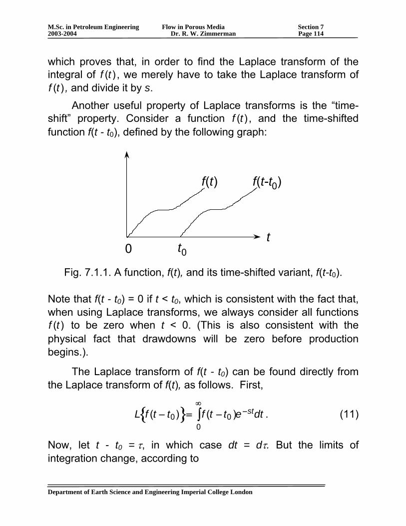
M.Sc. in Petroleum Engineering Flow in Porous Media Section 7 2003-2004 Dr. R. W. Zimmerman Page 114 which proves that, in order to find the Laplace transform of the integral of f (t) , we merely have to take the Laplace transform of f (t) , and divide it by s. Another useful property of Laplace transforms is the “time-shift” property. Consider a function f (t) , and the time-shifted function f(t - t0), defined by the following graph:
t0 t
f(t) f(t-t0)
0 Fig. 7.1.1. A function, f(t), and its time-shifted variant, f(t-t0).
Note that f(t - t0) = 0 if t < t0, which is consistent with the fact that, when using Laplace transforms, we always consider all functions f (t) to be zero when t < 0. (This is also consistent with the physical fact that drawdowns will be zero before production begins.).
The Laplace transform of f(t - t0) can be found directly from the Laplace transform of f(t), as follows. First,
L f (t − t0){ }= f (t − t0 )e −stdt
0
∞
∫ . (11)
Now, let t - t0 = τ, in which case dt = dτ. But the limits of integration change, according to
Department of Earth Science and Engineering Imperial College London
M.Sc. in Petroleum Engineering Flow in Porous Media Section 7 2003-2004 Dr. R. W. Zimmerman Page 115
τ = - t0 when t = 0, τ = ∞ when t = ∞ . (12)
Hence,
L f (t − t0){ }= f (τ )e−s(τ +t0 )dτ
−t0
∞
∫ . (13)
But f(τ) = 0 when τ < 0, so
L f (t − t0){ }= f (τ )e−s(τ +t0 )dτ
0
∞
∫ = f (τ )e−sτe−st0dτ0
∞
∫
= e−st0 f (τ )e−sτdτ
0
∞
∫ = e−st0 ÷ f (s). (14)
So, “delaying” a function f (t) by an amount of time t0 corresponds to multiplying its Laplace transform by e−st0 .
If we take a function f (t) , and “damp it out” by multiplying it by e-at, this is equivalent to replacing s with s+a in the Laplace transform of f (t) . The proof is as follows:
L e −at f(t){ }= f (t)e−at e−stdt0
∞
∫
= f (t)e−(s+a)tdt =0
∞
∫ ÷ f (s + a).
(15)
Finally, consider a function f(t), and the “stretched” function f(at). The Laplace transform of f(at) is related to the Laplace transform of f(t) as follows (see Tutorial Sheet 6):
{ } )~ s/afa
atfL (1)( = . (16)
Department of Earth Science and Engineering Imperial College London
M.Sc. in Petroleum Engineering Flow in Porous Media Section 7 2003-2004 Dr. R. W. Zimmerman Page 116 If we think of a as a frequency, as in the function sin(at), eq. (16) shows that “speeding up” a function by a factor a is essentially equivalent to “slowing down” its Laplace transform by the factor 1/a. The usefulness of the various rules presented above is that they minimise the number of times we actually have to calculate a Laplace transform via the basic definition (1). By knowing the Laplace transforms of a few functions, we can use these rules to calculate the Laplace transforms of other functions. For example, first note that if f (t) = 1, then
L f (t){ }= L 1{}= 1e−st
0
∞
∫ dt =−1s
e −st]0∞
=1s
. (17)
[Note: f (t) = 1 is a very well-behaved mathematical function, but its Laplace transform is not, since ∞→)(sf~ when s = 0. Points where )(sf~ becomes infinite, or is otherwise non-analytic (i.e., can’t be represented by a Taylor series), are known as singularities. The singularities of )(sf~ are actually the key to “inverting” ÷ f (s) in order to find the actual function, f (t) . However, we will not make use of these ideas, because they require knowledge of complex variable theory].
Now suppose that we want to calculate L{ f (t) } for the case of f(t) = t. We could use eq. (1), but it is easier to see from eq. (10) that, since t is the integral of 1, then L{t} can be found by dividing L{1} by s, i.e.,
L t{}= L 1dτ
0
t∫
⎧ ⎨ ⎩
⎫ ⎬ ⎭
= 1sL 1{}= 1
s2 . (18)
Department of Earth Science and Engineering Imperial College London
M.Sc. in Petroleum Engineering Flow in Porous Media Section 7 2003-2004 Dr. R. W. Zimmerman Page 117 A particular Laplace transform that is very useful in solving diffusion problems is L{t -1/2}:
L{t−1/2 } = t −1/ 2e −stdt
0
∞
∫ . (19)
To evaluate this integral, we let st = u, in which case dt = du/s, and the integral becomes
L{t−1/2 } = (u / s)−1/ 2e −u du
s0
∞
∫ =1s
u −1/2e−udu0
∞
∫ . (20)
Now put u = m2, in which case du = 2mdm = 2√udm, and so
L{t−1/2 } =
2s
e −m2dm0
∞
∫ =2s
π2
=πs
, (21)
which can also be expressed as
L−1{π1/ 2s−1/2 } = t −1/ 2 . (22)
By applying the rule that division by s in the Laplace domain corresponds to integration with respect to t in the time domain, we can show that
L−1{π1/ 2s−3/ 2} = τ −1/ 2
0
t∫ dτ = 2t1/ 2
⇒ L{t1/ 2} =π
2s3/ 2.
(23)
This process can be repeated to give, for n = 1,2,...:
Department of Earth Science and Engineering Imperial College London
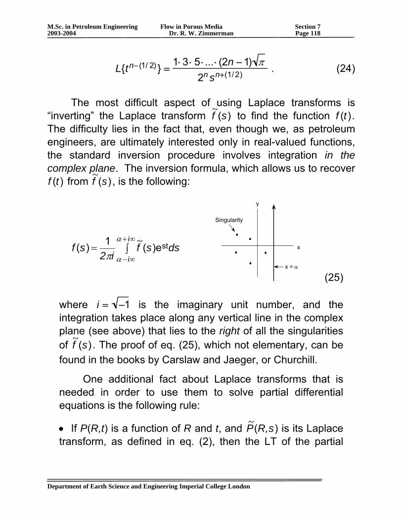
M.Sc. in Petroleum Engineering Flow in Porous Media Section 7 2003-2004 Dr. R. W. Zimmerman Page 118
L{tn− (1/ 2) } =
1⋅3 ⋅ 5 ⋅... ⋅ (2n − 1) π2n sn+(1/2)
. (24)
The most difficult aspect of using Laplace transforms is “inverting” the Laplace transform )(sf~ to find the function f (t) . The difficulty lies in the fact that, even though we, as petroleum engineers, are ultimately interested only in real-valued functions, the standard inversion procedure involves integration in the complex plane. The inversion formula, which allows us to recover f (t) from )(sf~ , is the following:
∫=∞+
∞−
i
i
α
απdssf
i2sf st)e(1)( ~
Singularity
x
y
x = α
(25)
where i = −1 is the imaginary unit number, and the integration takes place along any vertical line in the complex plane (see above) that lies to the right of all the singularities of )(sf~ . The proof of eq. (25), which not elementary, can be found in the books by Carslaw and Jaeger, or Churchill.
One additional fact about Laplace transforms that is needed in order to use them to solve partial differential equations is the following rule:
• If P(R,t) is a function of R and t, and )( sR,P~ is its Laplace transform, as defined in eq. (2), then the LT of the partial
Department of Earth Science and Engineering Imperial College London
M.Sc. in Petroleum Engineering Flow in Porous Media Section 7 2003-2004 Dr. R. W. Zimmerman Page 119 derivative of P with respect to R is equal to the partial derivative, with respect to R, of the LT of P, i.e.,
L dP
dR
⎧ ⎨ ⎩ ⎪
⎫ ⎬ ⎭ ⎪ =
ddR
L P(R,t){ }[ ]=d ÷ P (R,s)
dR. (26)
The proof of this fact follows directly from Leibnitz’s theorem for differentiating an integral with respect to a parameter that appears in the integrand:
L dP(R,t )dR
⎧ ⎨ ⎩ ⎪
⎫ ⎬ ⎭ ⎪
=dP(R,t)
dRe−stdt
0
∞
∫
=d
dRP(R,t)e −stdt
0
∞
∫ =d ÷ P (R,s)
dR.
(27)
In the second term we first differentiate with respect to R, and then integrate with respect to t, whereas in the third term we first integrate with respect to t, and then differentiate with respect to R. Leibnitz’ theorem says that the order in which we carry out these two operations is immaterial.
7.2. Flow to a hydraulically-fractured well
In general, exact inversion (as opposed to numerical inversion, which will be briefly discussed in section 7.4) of a Laplace transform requires knowledge of complex variable theory. One of the few important problems that we can solve with Laplace transforms without knowledge of complex integration is the one-dimensional diffusion equation in a semi-infinite region.
Department of Earth Science and Engineering Imperial College London
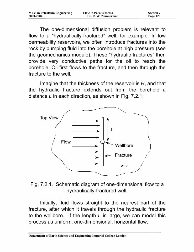
M.Sc. in Petroleum Engineering Flow in Porous Media Section 7 2003-2004 Dr. R. W. Zimmerman Page 120 The one-dimensional diffusion problem is relevant to flow to a “hydraulically-fractured” well, for example. In low permeability reservoirs, we often introduce fractures into the rock by pumping fluid into the borehole at high pressure (see the geomechanics module). These “hydraulic fractures” then provide very conductive paths for the oil to reach the borehole. Oil first flows to the fracture, and then through the fracture to the well.
Imagine that the thickness of the reservoir is H, and that the hydraulic fracture extends out from the borehole a distance L in each direction, as shown in Fig. 7.2.1:
z
Top View
Wellbore
Fracture
L
Flow
Fig. 7.2.1. Schematic diagram of one-dimensional flow to a hydraulically-fractured well.
Initially, fluid flows straight to the nearest part of the fracture, after which it travels through the hydraulic fracture to the wellbore. If the length L is large, we can model this process as uniform, one-dimensional, horizontal flow.
Department of Earth Science and Engineering Imperial College London
M.Sc. in Petroleum Engineering Flow in Porous Media Section 7 2003-2004 Dr. R. W. Zimmerman Page 121 The governing equation for this problem is the 1-D diffusion equation in Cartesian co-ordinates, eq. (1.6.8):
PDE: dPdt
= D d2Pdz2
, (1)
where z is the coordinate normal to the fracture plane, and D is the hydraulic diffusivity k /φμct .
If the total flowrate into the well is Q, and this flow is distributed uniformly over an area of 4LH (two fractures with two faces each), then the initial and boundary conditions are
IC: P(z,t = 0) = Pi , (2)
far-field BC: P(z → ∞,t) = Pi , (3)
fracture BC: dPdz
(z = 0,t ) =μQ
4kLH. (4)
(1) To solve this problem, we first define the LT of P(z,t):
∫≡∞
−
0)()( tdetz,Psz,P st~ . (5)
(2) Next, we take the Laplace transform of both sides of eq. (1). Using eq. (7.1.7), and eq. (2), the LHS of eq. (1) is transformed into:
L dP
dt
⎧ ⎨ ⎩ ⎪
⎫ ⎬ ⎭ ⎪ = sL{P(z,t )} − P(z,t = 0) = s ÷ P (z,s) − Pi . (6)
Department of Earth Science and Engineering Imperial College London
M.Sc. in Petroleum Engineering Flow in Porous Media Section 7 2003-2004 Dr. R. W. Zimmerman Page 122 Applying rule (7.1.26) twice, the Laplace transform of the RHS of eq. (1) is
L D d2P
dz2
⎧ ⎨ ⎪
⎩ ⎪
⎫ ⎬ ⎪
⎭ ⎪ = D d 2
dz2 L P(z,t){ }[ ]= D d 2 ÷ P (z,s)dz2 . (7)
So, the transformed representation of eq. (1) is
ODE: D d2 ÷ P (z,s)
dz2− s ÷ P (z,s) = −Pi . (8)
Although )( sz,P~ is a function of two variables, z and s, there are no derivatives of )( sz,P~ with respect to s in eq. (8). So s really appears in eq. (8) as a parameter, not a variable. Consequently, eq. (8) is an ODE rather than a PDE. The initial condition is already incorporated into eq. (8). However, we must now take the Laplace transforms of the two BCs, eqs. (3) and (4):
• far-field BC:
L{P(z = ∞,t)} = ÷ P (z = ∞,s) = L{Pi } =
Pis
, (9)
• fracture BC:
L dP
dz(z = 0,t)
⎧ ⎨ ⎩ ⎪
⎫ ⎬ ⎭ ⎪ =
d ÷ P dz
(z = 0,s) = L μQ4kLH
⎧ ⎨ ⎩ ⎪
⎫ ⎬ ⎭ ⎪ =
μQ4kLHs
. (10)
(3) Next, we solve the problem in the Laplace domain. The general solution to eq. (8) is
÷ P (z,s) = Aez s / D + Be−z s /D +
Pis
, (11)
where A and B are arbitrary constants. Department of Earth Science and Engineering Imperial College London
M.Sc. in Petroleum Engineering Flow in Porous Media Section 7 2003-2004 Dr. R. W. Zimmerman Page 123 The far-field boundary condition, eq. (9), shows that A must be zero. The fracture BC, eq. (10), implies that
d ÷ P dz
(z = 0,s) = −B s / D =μQ
4kLHs,
⇒ B =
−μQ4kLHs s / D
. (12)
So, the solution to this problem in the Laplace domain is
÷ P (z,s) =
Pis
−μQ D
4kLHs3/ 2e −z s / D . (13)
(4) Finally, we must invert ÷ P (z,s) to find P(z,t). To keep the analysis simple and brief, we will only invert for the pressure in the fracture, P(z=0,t).
Note: This illustrates another advantage of Laplace transform methods: we can usually find the wellbore pressure without having to find the pressure at every point in the reservoir; with other methods, you must find P(z,t) first as a complete function, and then set z = 0.
So, ÷ P (z = 0,s) =
Pis
−μQ D
4kLHs3 / 2. (14)
We now “invert” to find P(z=0,t), using eqs. (7.1.17,23):
P(z = 0,t) = L−1{ ÷ P (z = 0,s)} = L−1 Pi
s−
μQ D4kLHs3/ 2
⎧ ⎨ ⎪
⎩ ⎪
⎫ ⎬ ⎪
⎭ ⎪
Department of Earth Science and Engineering Imperial College London
M.Sc. in Petroleum Engineering Flow in Porous Media Section 7 2003-2004 Dr. R. W. Zimmerman Page 124
= Pi L−1 1
s⎧ ⎨ ⎩ ⎪
⎫ ⎬ ⎭ ⎪ −
μQ D4kLH
L−1 1s3 /2
⎧ ⎨ ⎩ ⎪
⎫ ⎬ ⎭ ⎪
= Pi −
μQ2kLH
Dtπ
. (15)
But, if the permeability of the fracture is much greater than that of the reservoir (which is the idea behind hydraulic fractures!), then there will be very little pressure drop in the fracture itself, and the fracture pressure will be equal to the wellbore pressure.
So, eq. (15) shows that the (early-time) drawdown in a fractured well should increase in proportion to t1/2.
7.3. Convolution principle in Laplace space
The convolution integral that appeared in eq. (3.4.6) is a particular case of a more general mathematical operation that can be defined by
f ∗ g ≡ f (τ )g(t − τ )dτ
0
t
∫ , (1)
and which is known as the convolution of f and g.
If we let t - τ = x in eq. (1), then τ = t - x and dτ = - dx, and the limits of integration are transformed into x = t and x = 0. Hence,
f ∗ g = − f(t − x )g(x)dx
t
0
∫ = f (t − x)g(x )dx ≡ g ∗ f0
t
∫ , (2)
which shows that f ∗ g = g ∗ f .
Department of Earth Science and Engineering Imperial College London
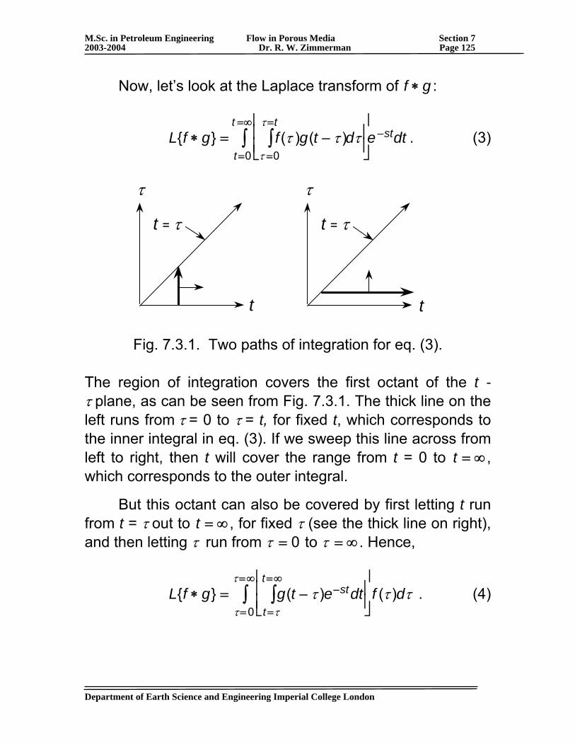
M.Sc. in Petroleum Engineering Flow in Porous Media Section 7 2003-2004 Dr. R. W. Zimmerman Page 125 Now, let’s look at the Laplace transform of f ∗ g :
L{f ∗ g} = f(τ )g(t − τ )dτ
τ =0
τ =t
∫⎡
⎣ ⎢ ⎢
⎤
⎦ ⎥ ⎥
t =0
t =∞
∫ e −stdt . (3)
t
τ
t = τ
t
τ
t = τ
Fig. 7.3.1. Two paths of integration for eq. (3).
The region of integration covers the first octant of the t - τ plane, as can be seen from Fig. 7.3.1. The thick line on the left runs from τ = 0 to τ = t, for fixed t, which corresponds to the inner integral in eq. (3). If we sweep this line across from left to right, then t will cover the range from t = 0 to t = ∞ , which corresponds to the outer integral.
But this octant can also be covered by first letting t run from t = τ out to t = ∞ , for fixed τ (see the thick line on right), and then letting τ run from τ = 0 to τ = ∞ . Hence,
L{f ∗ g} = g(t − τ )e−stdt
t =τ
t =∞
∫⎡
⎣ ⎢ ⎢
⎤
⎦ ⎥ ⎥
τ =0
τ =∞
∫ f (τ )dτ . (4)
Department of Earth Science and Engineering Imperial College London
M.Sc. in Petroleum Engineering Flow in Porous Media Section 7 2003-2004 Dr. R. W. Zimmerman Page 126 If we now let t - τ = x in eq. (4), then t = τ + x, dt = dx, and the limits of integration of the inner integral are transformed into x = 0 and x = ∞ :
L{f ∗ g} = g(x)e−s(τ +x)dxx=0
x=∞
∫⎡
⎣ ⎢ ⎢
⎤
⎦ ⎥ ⎥
τ =0
τ =∞
∫ f(τ )dτ
= f (τ )e−sτdτ g(x)e−sxdxx=0
x=∞
∫⎡
⎣ ⎢ ⎢
⎤
⎦ ⎥ ⎥
τ =0
τ =∞
∫ = ÷ f (s) ÷ g (s).
(5)
We have therefore proven that convolution of two functions in the time domain corresponds to multiplication of the their respective Laplace transforms. This is extremely useful, because (a) It implies that, if we can break up a difficult Laplace transform into the product of two simpler transforms whose inverses are known, then we can find the complete inverse function by convolution. (b) More importantly, it implies that, for any given reservoir geometry, if we can solve the diffusion equation for the case of a constant production rate, then the solution for an arbitrary production schedule can be found by convolution. Actually, we already knew this from section 3.4. However, the concept is more general, since, for example, we can also use it to find the solution for the case of varying wellbore pressure from the solution for the case of constant wellbore pressure. As an example of the use of convolution in the Laplace domain, consider the hydraulic fracture problem of section 7.2, but with an arbitrary time-dependent flowrate into the
Department of Earth Science and Engineering Imperial College London
M.Sc. in Petroleum Engineering Flow in Porous Media Section 7 2003-2004 Dr. R. W. Zimmerman Page 127 fracture, Q(t). The only change in the formulation of the problem will be in the fracture boundary condition, eq. (7.2.4), which now becomes
dPdz
(z = 0,t ) =μQ(t )4kLH
. (6)
If we follow the solution procedure used in section 7.2, the only change occurs when we take the Laplace transform of this boundary condition, in which case μQ / 4kLHs is replaced with the more general expression μ ÷ Q (s) / 4kLH . The solution in Laplace space then becomes
÷ P (z,s) =
Pis
−μ ÷ Q (s) D4kLHs1/ 2
e−z s / D . (7)
We again restrict our attention to the fracture, where z = 0:
÷ P (z = 0,s) =
Pis
−μ ÷ Q (s) D4kLHs1/ 2
. (8)
We now take the inverse Laplace transform, and in doing so make use of linearity and convolution:
P(z = 0,t) = L−1 ÷ P (z = 0,s){ }= L−1 Pi
s−
μ ÷ Q (s) D4kLHs1/2
⎧ ⎨ ⎪
⎩ ⎪
⎫ ⎬ ⎪
⎭ ⎪
= Pi L−1 1
s⎧ ⎨ ⎩ ⎪
⎫ ⎬ ⎭ ⎪ −
μ D4kLH
L−1÷ Q (s)s1/ 2
⎧ ⎨ ⎪
⎩ ⎪
⎫ ⎬ ⎪
⎭ ⎪
= Pi −
μ D4kLH
L−1{ ÷ Q (s)}[ ]∗ L−1{s−1/ 2 }[ ]. (9)
Department of Earth Science and Engineering Imperial College London
M.Sc. in Petroleum Engineering Flow in Porous Media Section 7 2003-2004 Dr. R. W. Zimmerman Page 128
But, L−1{ ÷ Q (s)} = Q(t ), by definition, and L−1{s−1/2 } = (πt)−1/ 2
by eq. (7.1.22), so
P(z = 0,t) = Pi − μ D
4kLH[Q(t)]∗[(πt)−1/2]
= Pi −
μ D / π4kLH
Q(τ )t − τ0
t∫ dτ
= Pi −
14LH
μπkφc
Q(τ )t − τ0
t∫ dτ
= Pi −
1A
μπkφc
Q(τ )t − τ0
t∫ dτ
= Pi −
μπkφc
q(τ )t − τ0
t∫ dτ . (10)
Eq. (10) gives us the pressure in the fracture as a function of the time-varying flowrate per unit area, q(t) = Q(t)/A.
Although it may be difficult to evaluate this integral analytically for some particular q(t), it will always be straightforward to evaluate it numerically. Convolution leads to an integral over time, which is a real variable, and such integrals are generally easier to evaluate than the complex integral specified in eq. (7.1.24).
Department of Earth Science and Engineering Imperial College London
M.Sc. in Petroleum Engineering Flow in Porous Media Section 7 2003-2004 Dr. R. W. Zimmerman Page 129 7.4. Numerical inversion of Laplace transforms
The complex integral that allows us to invert the Laplace transform of the pressure to obtain the pressure as a function of time is often very difficult to evaluate in closed form. Consequently, numerous algorithms have been devised to carry out this inversion numerically. Their use in petroleum engineering problems is reviewed in the book Fundamental and Applied Pressure Analysis by Daltaban and Wall (Imperial College Press, 1998). The most widely-used numerical algorithm for inverting a Laplace transform is the Stehfest algorithm. Although the derivation of this algorithm is very lengthy, and beyond the scope of this course, we can gain a rough understanding of it as follows. In general, any integral can be approximated by a summation whose terms consist of the integrand evaluated at various discrete points, which each functional evaluation multiplied by an appropriate weighting factor. For example, consider a simple numerical approximation of an integral based on the trapezium rule. Imagine a function f(x), which we want to integrate from x = a to x = b. Recall that an integral can be interpreted as the area under the graph of the function.
The area under the graph of f(x) can be approximated by the area of the trapezium shown in Fig. 7.4.1, i.e.,
f (x)dx
a
b
∫ ≈f(a) + f (b)
2
⎡
⎣ ⎢ ⎢
⎤
⎦ ⎥ ⎥ (b − a) . (1)
Department of Earth Science and Engineering Imperial College London
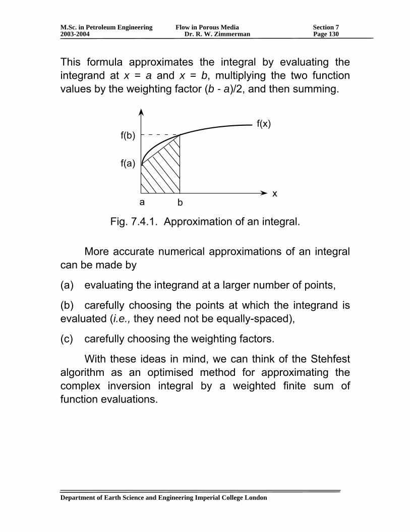
M.Sc. in Petroleum Engineering Flow in Porous Media Section 7 2003-2004 Dr. R. W. Zimmerman Page 130 This formula approximates the integral by evaluating the integrand at x = a and x = b, multiplying the two function values by the weighting factor (b - a)/2, and then summing.
a bx
f(x)
f(a)
f(b)
Fig. 7.4.1. Approximation of an integral.
More accurate numerical approximations of an integral can be made by
(a) evaluating the integrand at a larger number of points,
(b) carefully choosing the points at which the integrand is evaluated (i.e., they need not be equally-spaced),
(c) carefully choosing the weighting factors.
With these ideas in mind, we can think of the Stehfest algorithm as an optimised method for approximating the complex inversion integral by a weighted finite sum of function evaluations.
Department of Earth Science and Engineering Imperial College London
M.Sc. in Petroleum Engineering Flow in Porous Media Section 7 2003-2004 Dr. R. W. Zimmerman Page 131 ● Actually, the situation is a bit more subtle than this, because the Stehfest method also manages to avoid evaluating )(sf~ at complex values of s, as would seem to be required by the path of integration shown in eq. (7.1.25); instead, the method requires only that the function )(sf~ be evaluated at real values of s.
● If we could perform the complex inversion integration analytically, we would arrive at a single mathematical equation that is valid for all values of t. On the other hand, if we use a numerical procedure, we must perform a new calculation for each value of t at which we want to know the pressure.
If we have the Laplace transform of, say, the wellbore pressure )(w sP~ , the actual wellbore pressure at time t is given, according to Stehfest, by
⎟⎠⎞
⎜⎝⎛ =∑=
= tnlnsPV
tlntP w
N
nnw
22)(2
1
~ , (2)
where the weighting factors Vn are defined by
Vn = (−1)n k N(2k)!
(N − k)!k!(k − 1)!(n − k)!(2k − n)!k= (n+1) /2
min(n,N )∑ . (3)
In principle, the accuracy of the approximation should increase as the number of terms in the series, which is 2N, increases. In practice, if too many terms are taken, accumulated round-off error begins to overshadow the additional accuracy. It has generally been found that an optimum value of 2N is about 18. Department of Earth Science and Engineering Imperial College London
M.Sc. in Petroleum Engineering Flow in Porous Media Section 7 2003-2004 Dr. R. W. Zimmerman Page 132 ______________________________________________
Tutorial Sheet 6:
(1) What is the Laplace transform of the function f(t) = e-at?
(2) Starting with the basic definition of the Laplace transform, eq. (7.1.1), verify eq. (7.1.16).
(3) Following the steps that were taken in section 7.2, use Laplace transforms to try to solve the one-dimensional diffusion problem with a constant-pressure boundary condition:
PDE: 1D
dPdt
=d2Pdz2
, (i)
IC: P(z,t = 0) = Pi , (ii)
far-field BC: P(z → ∞,t) = Pi , (iii)
fracture BC: P(z = 0,t) = Pf . (iv)
(a) Find the solution for the pressure in the Laplace domain, i.e., find s)(z,P~ .
(b) Find, in the Laplace domain, an expression for the flowrate into the fracture; call it (s)Qf
~ .
(c) Invert (s)Qf~ to find the flowrate into the fracture as a
function of time, Qf (t).
Department of Earth Science and Engineering Imperial College London
M.Sc. in Petroleum Engineering Flow in Porous Media Section 8 2003-2004 Dr. R. W. Zimmerman Page 133
8. Naturally-Fractured Reservoirs Many reservoirs contain a network of interconnected naturally occurring fractures that provide most of the reservoir-scale permeability. In fact, it has been estimated that about 40% of the world’s known reserves occur in fractured reservoirs. Flow through such reservoirs is more complicated than through unfractured reservoirs, and cannot be analysed with the equations that we have developed and solved in the previous sections. The basic mathematical model used for fractured reservoirs was first developed by Barenblatt, Zheltov and Kochina in 1960, and by Warren and Root in 1963 (SPEJ, 1963). Several refinements have been made since then, and the resulting equations have been solved for many different reservoir geometries, with and without wellbore storage, skin effects, etc. In this section we will briefly describe this model, and present and discuss the solution for flow to a well in an unbounded dual-porosity reservoir.
8.1. Dual-porosity model of Barenblatt et al. In this model, the permeability of the reservoir is assumed to be provided solely by the fracture network. The regions of rock between the fractures, called “matrix blocks”, store most of the fluid, and feed this fluid into the fractures. The first step in constructing a mathematical model for dual-porosity media is to start with a pressure diffusion equation for the fracture network. In radial co-ordinates, this equation takes the form
(φc)f
dPfdt
=kfμ
1R
ddR
R dPfdR
⎛
⎝ ⎜ ⎜
⎞
⎠ ⎟ ⎟ + qmf , (1)
Department of Earth Science and Engineering Imperial College London
M.Sc. in Petroleum Engineering Flow in Porous Media Section 8 2003-2004 Dr. R. W. Zimmerman Page 134
where the subscript f denotes the properties of the fracture network, and the term qmf represents the volumetric flux of fluid from the matrix blocks into the fractures, per unit time and per unit volume of the reservoir. The “fracture-matrix interaction term” qmf
therefore has dimensions of , or [1/s]. [m3 /m3s]
Note: in a dual-porosity model, every point “R” is supposed to represent an REV (see section 1.3) that is large enough to encompass several fractures and matrix blocks.
The fracture-matrix flow term could be found by solving a flow equation in the matrix blocks, as has been done by Kazemi (SPEJ, 1969) and others. However, most dual-porosity formulations follow Barenblatt et al. and assume that the flow from the matrix blocks to the fractures, at point R in the reservoir, is proportional to the difference between the pressure in the fractures and the average pressure in the matrix blocks, P m; this is called “pseudo-steady-state fracture/matrix flow”. The flow should also be proportional to the permeability of the matrix, and inversely proportional to the fluid viscosity, so qmf is assumed to have the form
qmf =
αkmμ
(P m − Pf ) , (2)
where α is a “shape factor” that accounts for the size and shape of the matrix block.
Dimensional analysis shows that α must have dimensions of , or in SI units. The precise value of α for a matrix
block of a given shape is found by calculating the smallest eigenvalue of the diffusion equation inside the matrix block. The shape factors for a few simple, idealised geometries are as follows (Zimmerman et al., Water Resources Research, 1993):
[1/L2] [1/ m2 ]
Department of Earth Science and Engineering Imperial College London
M.Sc. in Petroleum Engineering Flow in Porous Media Section 8 2003-2004 Dr. R. W. Zimmerman Page 135
• spherical block of radius a:
α =π 2
a2 , (3)
• long cylindrical block of radius a:
α =
5.78a2
, (4)
• cubical block of side L:
α =
3π 2
L2 , (5)
• rectangular block of sides {Lx,Ly ,Lz } :
α = π 2 1
Lx2
+1
Ly2
+1Lz
2
⎡
⎣ ⎢ ⎢
⎤
⎦ ⎥ ⎥ . (6)
If the fracture system in the reservoir consists of three mutually orthogonal sets of parallel fractures, with spacings
{Lx,Ly ,Lz } , then the matrix blocks would be rectangular slabs; hence this last model, although simplified, is not unrealistic.
Eqs. (1,2) give two equations for three unknowns, {Pf ,P m,qmf } . Three equations are needed in order to find a solution. The third equation is found by performing a mass-balance on the matrix blocks. In analogy with eq. (6.3.16), we find
qmf = −(φc)m
dPmdt
. (7)
Eqs. (1,2,7) give a complete set of equations that can be solved for the unknown pressures and flowrates.
Department of Earth Science and Engineering Imperial College London
M.Sc. in Petroleum Engineering Flow in Porous Media Section 8 2003-2004 Dr. R. W. Zimmerman Page 136
8.2. Dual-porosity equations in dimensionless form
Before presenting the solution to the problem of constant flowrate to a well in a dual-porosity reservoir, it is convenient to first write the governing equations in dimensionless form.
We define the following dimensionless variables:
Dimensionless time:
tD =
kf t(φfcf + φmcm )μRw
2 ; (1)
this is the “standard” definition, but based on the reservoir-scale permeability, which is kf, and the total storativity, which is the sum of fracture storativity plus the matrix storativity.
Dimensionless pressure in the fractures:
PDf =
2πkf H(Pi − Pf )μQ
; (2)
this is again the standard definition, as in section 2.2.
Dimensionless pressure in the matrix blocks:
PDm =
2πkf H(Pi − P m )μQ
; (3)
this definition is based on kf, rather than km, so as to be consistent with the definition of PDf.
Dimensionless radius:
RD =
RRw
; (4)
which is the standard definition we have used previously for single-porosity reservoirs.
Department of Earth Science and Engineering Imperial College London

M.Sc. in Petroleum Engineering Flow in Porous Media Section 8 2003-2004 Dr. R. W. Zimmerman Page 137
We now use these definitions, along with the chain rule, to transform eqs. (8.1.1,2,7) into dimensionless form. We start with the left-hand side of eq. (8.1.1):
(φc)f
dPfdt
= (φc)fdPf
dPDf⋅dPDfdtD
⋅dtDdt
= (φc)f
−μQ2πkf H
⎡
⎣ ⎢ ⎢
⎤
⎦ ⎥ ⎥
dPDfdtD
kf
(φfcf + φmcm )μRw2
⎡
⎣ ⎢ ⎢
⎤
⎦ ⎥ ⎥
= −
φfcfQ(φfcf + φmcm )2πHRw
2
⎡
⎣ ⎢ ⎢
⎤
⎦ ⎥ ⎥
dPDfdtD
. (5)
Applying the same procedure to the spatial derivative term in eq. (8.1.1) gives
kfμ
1R
ddR
R dPfdR
⎛
⎝ ⎜ ⎜
⎞
⎠ ⎟ ⎟ =
−Q2πHRw
21
RD
ddRD
RDdPDfdRD
⎛
⎝ ⎜ ⎜
⎞
⎠ ⎟ ⎟ . (6)
Lastly, we transform the qmf term in eq. (8.1.1), using eq. 8.1.7). In analogy with eq. (5), this term becomes
qmf = −(φc)m
dP mdt
=φmcmQ
(φf cf + φmcm )2πHRw2
⎡
⎣ ⎢ ⎢
⎤
⎦ ⎥ ⎥ dPDmdtD
. (7)
Inserting eqs. (5,6,7) into eq. (8.1.1) yields
1RD
ddRD
RDdPDfdRD
⎛
⎝ ⎜ ⎜
⎞
⎠ ⎟ ⎟ =
φf cf(φf cf +φmcm )
dPDfdtD
+φmcm
(φfcf +φmcm)dPDmdtD
. (8)
Eq. (8) is the dimensionless form of eq. (8.1.1).
Department of Earth Science and Engineering Imperial College London
M.Sc. in Petroleum Engineering Flow in Porous Media Section 8 2003-2004 Dr. R. W. Zimmerman Page 138
We now write eq. (8.1.2) in terms of the dimensionless variables:
qmf =
αkmμ
(P m − Pf ) =−αkmQ2πkf H
(PDm − PDf ) . (9)
Equating this result to eq. (7) gives
φmcm(φf cf + φmcm )
dPDmdtD
=αkmRw
2
kf(PDf − PDm) . (10)
Eqs. (8,10) are two coupled differential equations for the two dimensionless pressures, PDf and PDm.
These two equations contain two dimensionless parameters. The first is the ratio of fracture storativity to total (fracture + matrix) storativity, known as ω:
ω =
φf cf(φf cf + φmcm )
. (11)
The second dimensionless parameter, λ, is essentially a ratio of matrix permeability to fracture permeability:
λ =
αkmRw2
kf . (12)
In practice, we usually have ω < 0.1, and λ < 0.001.
In terms of these dimensionless parameters ω and λ, and the dimensionless variables defined in eqs. (1-4), the two governing equations for a dual-porosity reservoir are
1RD
ddRD
RDdPDfdRD
⎛
⎝ ⎜ ⎜
⎞
⎠ ⎟ ⎟ = ω dPDf
dtD+ (1− ω )dPDm
dtD, (13)
Department of Earth Science and Engineering Imperial College London
M.Sc. in Petroleum Engineering Flow in Porous Media Section 8 2003-2004 Dr. R. W. Zimmerman Page 139
(1− ω ) dPDm
dtD= λ(PDf − PDm) . (14)
If the reservoir is actually a “single-porosity” reservoir, then the storativity ratio ω would be 1, and these two equations, (13) and (14), would reduce to the standard pressure diffusion equation, (6.1.8). In the usual form of the dual-porosity model, fluid does not flow from one matrix block to another. Only the fractures provide the macroscopic, reservoir-scale permeability. Hence, the pressure that we measure in the wellbore represents the pressure in those fractures that are nearest the wellbore. Therefore, the drawdown in the wellbore is found from
ΔPDw(tD)≡ PDf (RD =1,tD) . (15)
A more general model of naturally fractured reservoirs, in which fluid can also flow from one matrix block to another, is known as the “dual-permeability model”; it is used by hydrologists, but is not yet widely used in petroleum engineering.
8.3. Solution for a well in a dual-porosity reservoir Warren and Root (SPEJ, 1963) solved the problem of a well producing at constant flowrate Q in an unbounded dual-porosity reservoir, using Laplace transforms. They found that, if the dimensionless time satisfies the condition
tD > 100ω, (1)
(which usually covers the times that we are interested in), the dimensionless drawdown in the well is described by
Department of Earth Science and Engineering Imperial College London
M.Sc. in Petroleum Engineering Flow in Porous Media Section 8 2003-2004 Dr. R. W. Zimmerman Page 140
ΔPDw =
12
lntD + 0.8091+ Ei −λtDω(1− ω )
⎡
⎣ ⎢ ⎢
⎤
⎦ ⎥ ⎥
− Ei −λtD(1− ω)
⎡
⎣ ⎢ ⎢
⎤
⎦ ⎥ ⎥
⎧ ⎨ ⎪
⎩ ⎪
⎫ ⎬ ⎪
⎭ ⎪ . (2)
As usual, it is instructive to analyse the behaviour of the solution in the various time regimes. When tD is > 100ω, but is not “too large”, the variables inside the Ei functions in eq. (2) will still be small enough to use eq. (2.4.3), which says that, if x < 0.01,
−Ei(−x) ≈ −0.5772 − lnx (3)
Use of eq. (3) in eq. (2) yields
ΔPDw =
12
lntD + 0.8091+ ln λtDω(1− ω)
⎡
⎣ ⎢ ⎢
⎤
⎦ ⎥ ⎥
− ln λtD(1− ω )
⎡
⎣ ⎢ ⎢
⎤
⎦ ⎥ ⎥
⎧ ⎨ ⎪
⎩ ⎪
⎫ ⎬ ⎪
⎭ ⎪
=
12
ln tD + 0.8091+ ln λtD(1− ω )
⎡
⎣ ⎢ ⎢
⎤
⎦ ⎥ ⎥
− lnω − ln λtD(1− ω )
⎡
⎣ ⎢ ⎢
⎤
⎦ ⎥ ⎥
⎧ ⎨ ⎪
⎩ ⎪
⎫ ⎬ ⎪
⎭ ⎪
=
12
ln(tD /ω ) + 0.8091{ } . (4)
If we use eqs. (8.2.1,2,11) to convert the drawdown to dimensional form, we find
2πkf HΔPwμQ
=12
ln kf t[(φc)f + (φc)m]μRw
2⋅[(φc)f + (φc)m ]
(φc)f
⎡
⎣ ⎢ ⎢
⎤
⎦ ⎥ ⎥
+ 0.8091⎧ ⎨ ⎪
⎩ ⎪
⎫ ⎬ ⎪
⎭ ⎪
i.e., ΔPw =
μQ4πkf H
ln kf t(φμc)f Rw
2
⎡
⎣ ⎢ ⎢
⎤
⎦ ⎥ ⎥
+ 0.8091⎧ ⎨ ⎪
⎩ ⎪
⎫ ⎬ ⎪
⎭ ⎪ , (5)
Department of Earth Science and Engineering Imperial College London
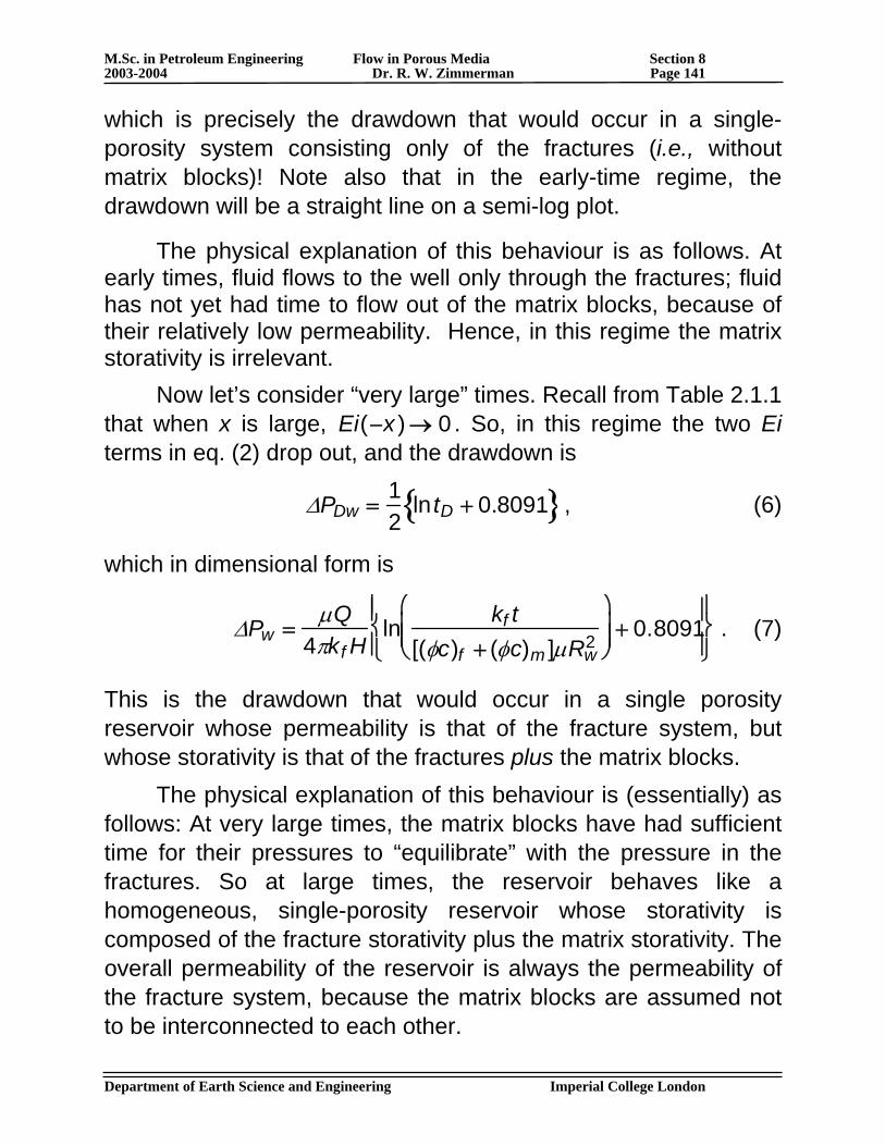
M.Sc. in Petroleum Engineering Flow in Porous Media Section 8 2003-2004 Dr. R. W. Zimmerman Page 141
which is precisely the drawdown that would occur in a single-porosity system consisting only of the fractures (i.e., without matrix blocks)! Note also that in the early-time regime, the drawdown will be a straight line on a semi-log plot.
The physical explanation of this behaviour is as follows. At early times, fluid flows to the well only through the fractures; fluid has not yet had time to flow out of the matrix blocks, because of their relatively low permeability. Hence, in this regime the matrix storativity is irrelevant. Now let’s consider “very large” times. Recall from Table 2.1.1 that when x is large, Ei(−x ) → 0 . So, in this regime the two Ei terms in eq. (2) drop out, and the drawdown is
ΔPDw =
12
ln tD + 0.8091{ } , (6)
which in dimensional form is
ΔPw =
μQ4πkf H
ln kf t[(φc)f + (φc)m ]μRw
2
⎛
⎝ ⎜ ⎜
⎞
⎠ ⎟ ⎟ + 0.8091
⎧ ⎨ ⎪
⎩ ⎪
⎫ ⎬ ⎪
⎭ ⎪ . (7)
This is the drawdown that would occur in a single porosity reservoir whose permeability is that of the fracture system, but whose storativity is that of the fractures plus the matrix blocks. The physical explanation of this behaviour is (essentially) as follows: At very large times, the matrix blocks have had sufficient time for their pressures to “equilibrate” with the pressure in the fractures. So at large times, the reservoir behaves like a homogeneous, single-porosity reservoir whose storativity is composed of the fracture storativity plus the matrix storativity. The overall permeability of the reservoir is always the permeability of the fracture system, because the matrix blocks are assumed not to be interconnected to each other.
Department of Earth Science and Engineering Imperial College London
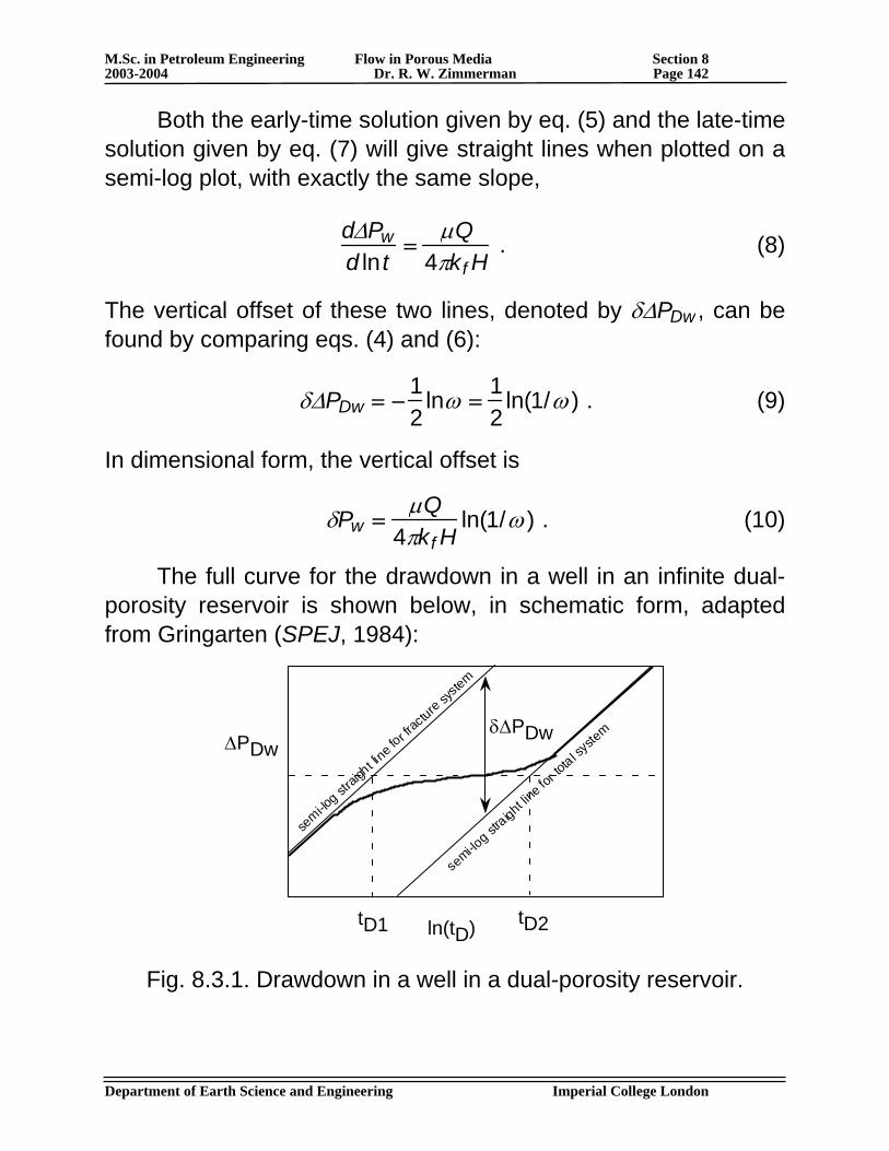
M.Sc. in Petroleum Engineering Flow in Porous Media Section 8 2003-2004 Dr. R. W. Zimmerman Page 142
Both the early-time solution given by eq. (5) and the late-time solution given by eq. (7) will give straight lines when plotted on a semi-log plot, with exactly the same slope,
dΔPwd ln t
=μQ
4πkf H . (8)
The vertical offset of these two lines, denoted by δΔPDw , can be found by comparing eqs. (4) and (6):
δΔPDw = −
12
lnω =12
ln(1/ω ) . (9)
In dimensional form, the vertical offset is
δPw =
μQ4πkf H
ln(1/ω ) . (10)
The full curve for the drawdown in a well in an infinite dual-porosity reservoir is shown below, in schematic form, adapted from Gringarten (SPEJ, 1984):
ln(tD)
ΔPDw
semi-lo
g strai
ght li
ne fo
r frac
ture s
ystem
semi-lo
g stra
ight lin
e for
tota l sys
tem
tD1 tD2
δΔPDw
Fig. 8.3.1. Drawdown in a well in a dual-porosity reservoir.
Department of Earth Science and Engineering Imperial College London
M.Sc. in Petroleum Engineering Flow in Porous Media Section 8 2003-2004 Dr. R. W. Zimmerman Page 143
Fig. 8.3.1 shows that there is a transition regime between the two semi-log straight lines. In this regime, the pressure drawdown changes very gradually. This regime is dominated by the effect of fluid beginning to flow out of the matrix blocks and into the fractures. During this regime, the flow from the matrix blocks into the fractures nearly compensates for the flow from the fractures into the borehole, and the wellbore pressure is (nearly) constant. Bourdet and Gringarten (SPE paper 9293, 1984) showed that if you draw a horizontal line through the drawdown curve at the midpoint between the two semi-log straight lines, this line will intersect the first semi-log straight line at a dimensionless time tD1 that is given by
tD1 = ω
γλ , (11)
where γ = 1.78 is Euler’s constant, and ω and λ are the two dual-porosity parameters defined in eqs. (8.2.11,12). This horizontal line intersects the late-time semi-log straight line at a dimensionless time tD2 given by
tD2 =
1γ λ
. (12)
Eqs. (11,12) show that the horizontal offset of the two asymptotic semi-log straight lines is equal to ln(1/ω). In dimensional form, these intercept times are
t1 =
(φμc)fα γ km
, (13)
t2 =
μ[(φc)f + (φc)m ]α γ km
. (14)
Department of Earth Science and Engineering Imperial College London
M.Sc. in Petroleum Engineering Flow in Porous Media Section 8 2003-2004 Dr. R. W. Zimmerman Page 144
The first intercept time, tD1, is essentially a measure of the time required for the volume of fluid that has been depleted from the matrix blocks near the wellbore to become of the same order of magnitude as the volume depleted from the fractures. The second intercept time, tD2, is a measure of the time required for the pressure in the matrix blocks nearest the well to come into equilibrium with the pressure in the surrounding fractures.
Eqs. (11) and (12) allow one to calculate the dual-porosity parameters ω and λ from well-test data, as will be demonstrated in the module on well test analysis.
______________________________________________
Tutorial Sheet 7:
(1) Without looking at the paper by Warren and Root, sketch the forms that you think the drawdown curve in Fig. 8.3.1 would have if
(a) The storativity ratio ω increased (or decreased) by a factor of 10.
(b) The permeability ratio λ increased (or decreased) by a factor of 10.
(2) By examining eq. (8.3.2), and making use of either eq. (2.1.22) or Table 2.1.1, derive an expression for the dimensionless time that must elapse in order for the approximation (8.3.6) to be accurate to within about 1%. Your answer should be in terms of the parameter λ.
Department of Earth Science and Engineering Imperial College London
M.Sc. in Petroleum Engineering Flow in Porous Media Section 9 2003-2004 Dr. R. W. Zimmerman Page 145
9. Flow of Gases in Porous Media 9.1. Diffusion equation for gas flow The main difference between analysing flow in gas reservoirs as opposed to liquid reservoirs is that, for gases, the governing partial differential equation becomes unavoidably nonlinear. The main reason for this nonlinearity is that, whereas the compressibility of a liquid can be assumed to be constant, and relatively small (in the sense that was quantified in section 1.6), the compressibility of a gas varies greatly with pressure. Furthermore, the viscosity of a gas also usually varies with pressure. The result is that the governing equation for gas flow cannot usually be well approximated by a linear diffusion equation with constant coefficients, as was the case for liquids.
To derive the governing equation for gas flow, we return to the analysis given in section 1.7, and note that, up to eq. (1.7.5), no assumptions were made about the magnitude of the compressibility. Hence, we can begin our analysis of gas flow with eq. (1.7.5):
−
d(ρqR)dR
= R d(ρφ )dt
. (1)
We now use Darcy’s law, in the form given by eq. (1.4.1), for the flux term q on the left-hand side, i.e.,
q = −
kμ
dPdR
, (2)
in which case eq. (1) takes the form
1R
ddR
ρkμ
R dPdR
⎛
⎝ ⎜ ⎜
⎞
⎠ ⎟ ⎟ =
d(ρφ)dt
. (3)
Department of Earth Science and Engineering Imperial College London
M.Sc. in Petroleum Engineering Flow in Porous Media Section 9 2003-2004 Dr. R. W. Zimmerman Page 146
We next note that the process of expressing the RHS of eq. (3) in terms of the pressure, which was carried out section 1.6, did not require any assumptions about the magnitude of the compressibility terms, etc. Hence, we can use eq. (1.6.1) to rewrite eq. (3) as
1R
ddR
ρkμ
R dPdR
⎛
⎝ ⎜ ⎜
⎞
⎠ ⎟ ⎟ = ρφ(Cf + Cφ ) dP
dt. (4)
Eq. (4) is completely general, in that it contains no assumption that the compressibility of the pore fluid is small. It also allows for the possibility that the density, permeability, and viscosity vary with pressure. As such, it is too general to be useful, except as the basis of a numerical solution. However, there are many cases of practical interest in which it can be either linearised, or “almost” linearised, in which case the standard solutions presented in the previous sections can be used.
9.2. Ideal gas, constant reservoir properties
One situation in which the nonlinear diffusion equation for gas flow can be effectively linearised is if the gas can be assumed to obey the ideal gas law:
P = ρRT , (1)
where R is the gas constant, and T is the absolute temperature. If we use eq. (1) to express the density in terms of the pressure, eq. (9.1.4) takes the form
1R
ddR
kPμRT
R dPdR
⎛
⎝ ⎜ ⎜
⎞
⎠ ⎟ ⎟ =
φ(Cf + Cφ )RT
P dPdt
. (2)
Department of Earth Science and Engineering Imperial College London
M.Sc. in Petroleum Engineering Flow in Porous Media Section 9 2003-2004 Dr. R. W. Zimmerman Page 147
The simplest model of gas flow can be derived from eq. (2) by making the following assumptions.
(a) Assume that the temperature is constant.
(b) Assume that the viscosity of the gas is independent of pressure. This is actually rigorously true for an ideal gas, for which the viscosity depends only on temperature. This assumption allows us to take μ outside of the derivative on the left-hand side of eq. (2).
(c) Assume that the compressibility of the gas is much larger than that of the formation, as is usually the case. In fact, the compressibility of an ideal gas is (1/P), since
Cf =
1ρ
dρdP
⎛
⎝ ⎜ ⎜
⎞
⎠ ⎟ ⎟
T=
RTP
ddP
PRT
⎛
⎝ ⎜ ⎜
⎞
⎠ ⎟ ⎟
T=
RTP
1RT
=1P
. (3)
As the reservoir pressure is usually less than 10,000 psi, the compressibility is at least 10−4/psi. The formation compressibility, on the other hand, is usually less than 10−5/psi (see Matthews and Russell, p. 159; Zimmerman, Compressibility of Sandstones, Elsevier, 1991). Hence, we can usually neglect C relative to φ Cf .
(d) Assume that the permeability of the formation is independent of the pore pressure. This is reasonably accurate for many reservoirs, but is sometimes not a very good assumption in fractured reservoirs or in tight gas sands, for example. This assumption allows us to take k outside of the derivative on the left-hand side of eq. (2).
Under these four assumptions, eq. (2) can be written as
Department of Earth Science and Engineering Imperial College London
M.Sc. in Petroleum Engineering Flow in Porous Media Section 9 2003-2004 Dr. R. W. Zimmerman Page 148
1R
ddR
RP dPdR
⎛
⎝ ⎜ ⎜
⎞
⎠ ⎟ ⎟ =
φμkP
P dPdt
. (4)
We now note that
P dP
dR=
12
d(P2)dR
, and P dPdt
=12
d(P2)dt
, (5)
which allows us to write eq. (4) as
1R
ddR
R d(P2)dR
⎛
⎝ ⎜ ⎜
⎞
⎠ ⎟ ⎟ =
φμkP
d(P2)dt
. (6)
Eq. (6) is the standard diffusion equation in radial coordinates, except that
(1) The dependent variable is P2 rather than P;
(2) The compressibility term, Ct ≈ Cf = 1/ P , varies with pressure.
Because of point (2), eq. (6) is still nonlinear, and is not quite equivalent to the diffusion equation used for liquid flow. However, we can linearise eq. (6) by evaluating the term P in the denominator of the RHS at either the initial pressure, Pi, or at the mean wellbore pressure during the test, i.e., at
Pm =
Pi + Pw(end of test)2
. (7)
If this is done, then eq. (6) becomes a linear diffusion equation, with P P
2 rather than P as the dependent variable.
Department of Earth Science and Engineering Imperial College London
M.Sc. in Petroleum Engineering Flow in Porous Media Section 9 2003-2004 Dr. R. W. Zimmerman Page 149
3. Real gas, variable reservoir properties
The ideal gas law is a good approximation to gas behaviour only at low pressures. It is also generally more accurate for monatomic or diatomic gases than for larger molecules such as gaseous hydrocarbons.
Hence, for gas reservoirs, which are usually at relatively high pressures, it is more accurate to replace the ideal gas law, eq. (9.2.1), with the “real gas” equation of state,
P = ρzRT, or ρ =
PzRT
, (1)
where z is the (dimensionless) gas deviation factor.
Using this equation of state, eq. (9.1.3) takes the form
1R
ddR
R kμzRT
P dPdR
⎛
⎝ ⎜ ⎜
⎞
⎠ ⎟ ⎟ = φ d
dtP
zRT
⎛
⎝ ⎜ ⎜
⎞
⎠ ⎟ ⎟ . (2)
Under isothermal conditions, this becomes
1R
ddR
R kμz
P dPdR
⎛
⎝ ⎜ ⎜
⎞
⎠ ⎟ ⎟ = φ d
dtPz
⎛
⎝ ⎜ ⎜
⎞
⎠ ⎟ ⎟ . (3)
Eq. (3) is highly nonlinear, but we can “partially linearise” it by defining a new variable, the “real gas pseudopressure”, as follows (see G. L. Chierici, Principles of Petroleum Reservoir Engineering, Vol. 1, Springer-Verlag, 1994, chapter 7):
m(P) = 2 k(P)P
μ(P)z(P)0
P∫ dP . (4)
Department of Earth Science and Engineering Imperial College London
M.Sc. in Petroleum Engineering Flow in Porous Media Section 9 2003-2004 Dr. R. W. Zimmerman Page 150
The real gas pseudopressure m(P) is just a generalisation of the P2 parameter that was used for ideal gases; this can be seen by noting that if we assume permeability and viscosity to be independent of pressure, and recall that z = 1 for an ideal gas, then
m(P) →
2kμ
P0
P∫ dP =
kμ
P2. (5)
Hence, for an ideal gas in a stress-insensitive reservoir, the pseudopressure m is, aside from a multiplicative constant, equal to P2. Returning to the real gas case, we differentiate eq. (4) with respect to P, to find
dm(P)dP
=2k(P)P
μ(P)z(P), (6)
which implies that
dmdR
=dmdP
dPdR
=2k(P)P
μ(P)z(P)dPdR
. (7)
Substituting eq. (7) into the left-hand side of eq. (3) leads to
12R
ddR
R dmdR
⎛
⎝ ⎜ ⎜
⎞
⎠ ⎟ ⎟ = φ d
dtPz
⎛
⎝ ⎜ ⎜
⎞
⎠ ⎟ ⎟ . (8)
The left-hand side of eq. (8) is essentially in the standard form for the diffusion equation. On the right-hand side, we recall that P / z = ρRT , so that under isothermal conditions,
Department of Earth Science and Engineering Imperial College London
M.Sc. in Petroleum Engineering Flow in Porous Media Section 9 2003-2004 Dr. R. W. Zimmerman Page 151
ddt
Pz
⎛
⎝ ⎜ ⎜
⎞
⎠ ⎟ ⎟ =
d(ρRT )dt
= RT dρdt
= RT dρdP
dPdt
. (9)
But from the definition of compressibility,
Cg =
1ρ
dρdP
⎛
⎝ ⎜ ⎜
⎞
⎠ ⎟ ⎟
T, so dρ
dP
⎛
⎝ ⎜ ⎜
⎞
⎠ ⎟ ⎟
T= ρCg , (10)
in which case eq. (9) can be written as
ddt
Pz
⎛
⎝ ⎜ ⎜
⎞
⎠ ⎟ ⎟ = RTρ(P)Cg (P) dP
dt. (11)
Next we recall from eq. (1) that ρ = P / zRT , and rewrite eq. (11) as
ddt
Pz
⎛
⎝ ⎜ ⎜
⎞
⎠ ⎟ ⎟ =
Cg(P)Pz(P)
dPdt
. (12)
Combining eq. (12) with eq. (8) yields
12R
ddR
R dmdR
⎛
⎝ ⎜ ⎜
⎞
⎠ ⎟ ⎟ =
φCg(P)Pz(P)
dPdt
. (13)
But by analogy with eq. (7), we have
dmdt
=2k(P)P
μ(P)z(P)dPdt
, (14)
so that
Department of Earth Science and Engineering Imperial College London

M.Sc. in Petroleum Engineering Flow in Porous Media Section 9 2003-2004 Dr. R. W. Zimmerman Page 152
dPdt
=μ(P)z(P)2k(P)P
dmdt
. (15)
Combining eq. (15) with eq. (13) yields
1R
ddR
R dmdR
⎛
⎝ ⎜ ⎜
⎞
⎠ ⎟ ⎟ =
φμ(P)Cg(P)k(P)
dmdt
. (16)
Eq. (16) is in the form of a standard diffusion equation in radial coordinates, except that the diffusivity term on the RHS is pressure-dependent.
As a final step in linearising the equation for gas flow to a well, we make the approximation that the diffusivity terms on the right can be replaced by some representative constant value, such as the value at the mean wellbore pressure encountered during a well test, i.e.,
1R
ddR
R dmdR
⎛
⎝ ⎜ ⎜
⎞
⎠ ⎟ ⎟ =
φμ(Pm )Cg (Pm )k(Pm )
dmdt
, (17)
where Pm is defined by eq. (9.2.7).
Eq. (17) is the (approximate) governing equation for the flow of real gases to a well. If the pressure-dependent terms on the RHS are evaluated at Pm, we can then use all of the standard solutions that have been developed for liquid flow, provided that we use m instead of P as the dependent variable.
The transformation between P and m is made by evaluating the integral that is given in eq. (4). If the reservoir is stress-sensitive, we would need to know k(P) to do this. Usually, we do not have this information. If we ignore the pressure-dependence of permeability, then the relationship between P and m becomes
Department of Earth Science and Engineering Imperial College London
M.Sc. in Petroleum Engineering Flow in Porous Media Section 9 2003-2004 Dr. R. W. Zimmerman Page 153
m(P) = 2k P
μ(P)z(P)0
P∫ dP . (18)
Since z(P) and μ(P) can be measured in the laboratory on samples of the reservoir gas, this integral can be evaluated a priori. The result is usually a relationship between m and P in tabular form, which is used to transform the measured pressures into values of m that are used in conjunction with our solutions to eq. (17).
9.4. Non-Darcy flow effects
All of the previous analyses have been based on Darcy’s law, which states that the flowrate is proportional to the pressure gradient. Darcy’s law is an empirical law that is known to hold only at low flowrates, which can be defined, roughly, as flows for which the Reynolds number is less than one. The Reynolds number is a dimensionless measure of the relative strengths of inertial forces relative to viscous forces. Using the definition of Reynolds number, this condition can be written as
Re =
ρvdμ
< 1, (1)
where ρ is the density of the fluid, μ is the viscosity, d is a mean pore diameter, and v is the mean (microscopic) velocity. It would be useful to be able to express this criterion in terms of macroscopically measurable quantities. If we use any of the common correlations between pore diameter and permeability, such as the following simplified form of the Kozeny-Carman equation,
k =
φd 2
96≈
φd 2
100, (2)
Department of Earth Science and Engineering Imperial College London
M.Sc. in Petroleum Engineering Flow in Porous Media Section 9 2003-2004 Dr. R. W. Zimmerman Page 154
we can express the pore diameter as
d = 10 k / φ . (3)
The criterion for Darcy’s law to be valid can therefore be written as
v <
μ φ10ρ k
. (4)
Next, we note that the macroscopic flowrate q must be equal to the microscopic flowrate v, multiplied by the porosity, i.e., q = vφ , so that
v =
qφ
. (5)
Hence, the criterion (4) for the validity of Darcy’s law can be written as
q <
μφ3 / 2
10ρ k. (6)
The total flowrate towards the well is related to the flux by
Q = Aq = 2πRHq , (7)
so condition (6) can be written as
Q <
2πRHμφ3/ 2
10ρ k≈
RHμφ3 / 2
ρ k, (8)
which is expressed solely in terms of our usual reservoir parameters.
Department of Earth Science and Engineering Imperial College London
M.Sc. in Petroleum Engineering Flow in Porous Media Section 9 2003-2004 Dr. R. W. Zimmerman Page 155
Criterion (8) becomes more stringent near the wellbore, because as a fixed volumetric flowrate gets channelled through a smaller area, the velocity must increase. If we use “typical” reservoir values in eq. (8), we would find that this criterion is usually violated for gas wells in the vicinity of the wellbore, but not for liquids, unless the flow is through fractures rather than pores. If the fluid is flowing through fractures, then the actual area available for flow is smaller, and the velocity of the fluid must be greater. In this case, it is more likely that the flow will be turbulent.
If criterion (8) is violated, Darcy’s law must be replaced with a nonlinear law such as Forchheimer’s equation:
dPdR
=μqk
+ βρq2, (9)
in which the coefficient β accounts for non-Darcy (inertial) effects. [In eq. (9), we assume that q is positive if it is towards the well].
Dimensional analysis of eq. (9) shows that the factor β has dimensions of L-1. As k has dimensions of L2 (recall eq. 2), it is roughly the case that β ≈ 1/ k . If this is true, then the magnitude of the nonlinear term in eq. (9) relative to that of the linear term is
ratio =
βρq2
(μq / k)=
βρqkμ
≈ρq k
μ. (10)
The term on the right of eq. (10) is essentially a Reynolds number based on a length scale of k . Hence, if the Reynolds number is much less than one, the nonlinear terms in eq. (9) are negligible, and we recover Darcy’s law.
The Forchheimer equation can be justified heuristically by noting that ρ q2 is related to the kinetic energy per unit volume of
Department of Earth Science and Engineering Imperial College London
M.Sc. in Petroleum Engineering Flow in Porous Media Section 9 2003-2004 Dr. R. W. Zimmerman Page 156
fluid, and the kinetic energy is not negligible at higher flowrates (recall eq. 1.1.2). Alternatively, one can interpret the Forchheimer equation as an empirical law.
Eq. (9) implies that the flowrate under a given pressure gradient will actually be less than would be predicted on the basis of Darcy’s law. Another way of interpreting eq. (9) is that, for a given flowrate, the pressure drop will be larger than that which would be predicted by Darcy’s law. Hence, non-Darcy effects can be said to contribute an “additional” pressure drop.
As non-Darcy flow is confined to a region near the wellbore, its effect during a well test is therefore somewhat similar to a “skin” effect. In fact, the main consequence of non-Darcy flow near the wellbore is that the skin factor gets “replaced” by an apparent skin factor, ′ s , which is given by
′ s = s + DQ, (11)
where D is the “non-Darcy skin coefficient”. This coefficient is related to the coefficient β that appears in Forchheimer’s equation (see Chierici, p. 241, for the details).
9.5. Klinkenberg effect
Liquids, as well as gases at typical reservoir pressures, behave like continua, in the sense that we can ignore the motions of individual molecules, and instead work with mean velocities that are averaged over a (very) large number of molecules. This leads to continuum-type theories such as Darcy’s law for flow through porous media, or the Navier-Stokes equations for fluid flow on the pore scale.
Department of Earth Science and Engineering Imperial College London
M.Sc. in Petroleum Engineering Flow in Porous Media Section 9 2003-2004 Dr. R. W. Zimmerman Page 157
A fundamental aspect of the Navier-Stokes equations is that the fluid velocity is assumed to be zero at the boundary with a solid - such as at the pore walls. This obviously must be true for the normal component of the velocity, but it is in fact also true for the tangential component. This boundary condition is the main reason why the N-S equations average out (“upscale”) to yield Darcy’s law. However, this micro-scale boundary condition will not hold for a gas at very low densities, which is to say at very low pressures. The reasons are complicated, but they boil down to the fact that in order for the gas to behave like a continuum, a given gas molecule must collide much more frequently with other gas molecules than with the pore walls. To quantify whether or not this will be the case, we must consider the concept of the “mean free path”, which is essentially the mean distance travelled by a molecule between subsequent collisions with other molecules. According to the kinetic theory of gases (see Molecular Theory of Gases and Liquids, Hirschfelder, Curtiss, and Bird, Wiley & Sons, 1954), the mean free path λ is essentially given by
λ =
12nπσ 2
=kBT
2πσ 2P, (1)
where n is the molecular density in molecules/volume, kB is the Boltzmann constant (i.e., the gas constant per molecule), and σ is an effective molecular diameter. If the pore size is smaller than the mean free path, collisions with the pore walls will be much more frequent than collisions with other molecules, and the gas will essentially flow through the pores as individual molecules, rather than as a fluid continuum. This type of flow is known as “Knudsen flow”, or “slip flow”.
Department of Earth Science and Engineering Imperial College London
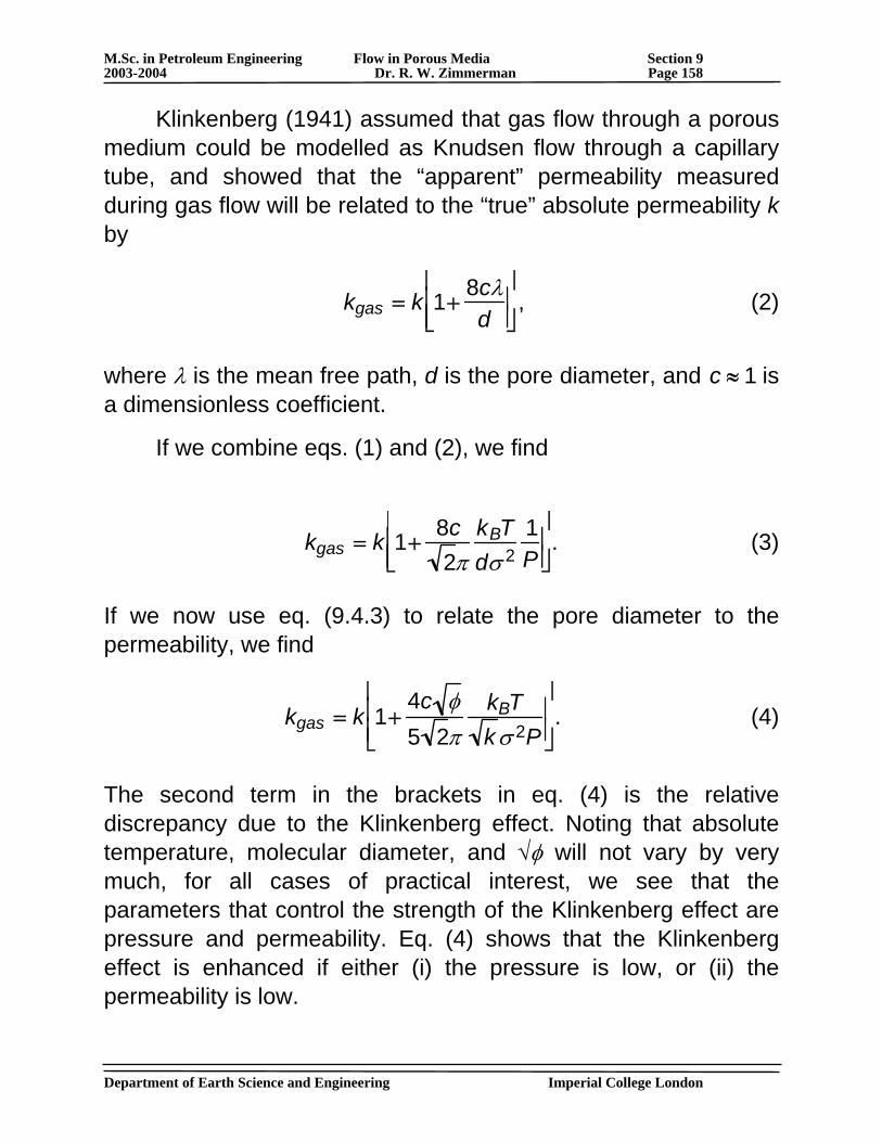
M.Sc. in Petroleum Engineering Flow in Porous Media Section 9 2003-2004 Dr. R. W. Zimmerman Page 158
Klinkenberg (1941) assumed that gas flow through a porous medium could be modelled as Knudsen flow through a capillary tube, and showed that the “apparent” permeability measured during gas flow will be related to the “true” absolute permeability k by
kgas = k 1+
8cλd
⎡
⎣ ⎢ ⎢
⎤
⎦ ⎥ ⎥ , (2)
where λ is the mean free path, d is the pore diameter, and c ≈ 1 is a dimensionless coefficient.
If we combine eqs. (1) and (2), we find
kgas = k 1+
8c2π
kBTdσ 2
1P
⎡
⎣ ⎢ ⎢
⎤
⎦ ⎥ ⎥ . (3)
If we now use eq. (9.4.3) to relate the pore diameter to the permeability, we find
kgas = k 1+
4c φ5 2π
kBTkσ 2P
⎡
⎣ ⎢ ⎢
⎤
⎦ ⎥ ⎥ . (4)
The second term in the brackets in eq. (4) is the relative discrepancy due to the Klinkenberg effect. Noting that absolute temperature, molecular diameter, and √φ will not vary by very much, for all cases of practical interest, we see that the parameters that control the strength of the Klinkenberg effect are pressure and permeability. Eq. (4) shows that the Klinkenberg effect is enhanced if either (i) the pressure is low, or (ii) the permeability is low.
Department of Earth Science and Engineering Imperial College London
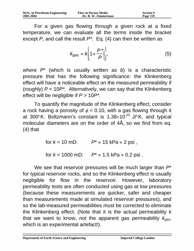
M.Sc. in Petroleum Engineering Flow in Porous Media Section 9 2003-2004 Dr. R. W. Zimmerman Page 159
For a given gas flowing through a given rock at a fixed temperature, we can evaluate all the terms inside the bracket except P, and call the result P*. Eq. (4) can then be written as
kgas = k 1+
P *P
⎡
⎣ ⎢ ⎢
⎤
⎦ ⎥ ⎥ , (5)
where P* (which is usually written as b) is a characteristic pressure that has the following significance: the Klinkenberg effect will have a noticeable effect on the measured permeability if (roughly) P < 10P*. Alternatively, we can say that the Klinkenberg effect will be negligible if P > 10P*.
To quantify the magnitude of the Klinkenberg effect, consider a rock having a porosity of φ = 0.10, with a gas flowing through it at 300°K. Boltzmann’s constant is 1.38×10⁻²³ J/°K, and typical molecular diameters are on the order of 4Å, so we find from eq. (4) that
for k = 10 mD: P* ≈ 15 kPa ≈ 2 psi ,
for k = 1000 mD: P* ≈ 1.5 kPa ≈ 0.2 psi .
We see that reservoir pressures will be much larger than P* for typical reservoir rocks, and so the Klinkenberg effect is usually negligible for flow in the reservoir. However, laboratory permeability tests are often conducted using gas at low pressures (because these measurements are quicker, safer and cheaper than measurements made at simulated reservoir pressures), and so the lab-measured permeabilities must be corrected to eliminate the Klinkenberg effect. (Note that it is the actual permeability k that we want to know, not the apparent gas permeability kgas, which is an experimental artefact!).
Department of Earth Science and Engineering Imperial College London
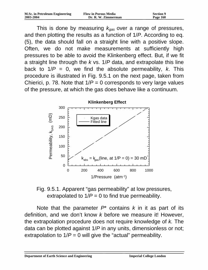
M.Sc. in Petroleum Engineering Flow in Porous Media Section 9 2003-2004 Dr. R. W. Zimmerman Page 160
This is done by measuring kgas over a range of pressures, and then plotting the results as a function of 1/P. According to eq. (5), the data should fall on a straight line with a positive slope. Often, we do not make measurements at sufficiently high pressures to be able to avoid the Klinkenberg effect. But, if we fit a straight line through the k vs. 1/P data, and extrapolate this line back to 1/P = 0, we find the absolute permeability, k. This procedure is illustrated in Fig. 9.5.1 on the next page, taken from Chierici, p. 78. Note that 1/P = 0 corresponds to very large values of the pressure, at which the gas does behave like a continuum.
0
50
100
150
200
250
300
0 200 400 600 800 1000
Klinkenberg Effect
Kgas dataFitted line
Per
mea
bilit
y, k
GAS
(m
D)
1/Pressure (atm-1)
kabs = kgas(line, at 1/P = 0) = 30 mD
Fig. 9.5.1. Apparent “gas permeability” at low pressures, extrapolated to 1/P = 0 to find true permeability.
Note that the parameter P* contains k in it as part of its definition, and we don’t know k before we measure it! However, the extrapolation procedure does not require knowledge of k. The data can be plotted against 1/P in any units, dimensionless or not; extrapolation to 1/P = 0 will give the “actual” permeability.
Department of Earth Science and Engineering Imperial College London