flow measurement handbook
TRANSCRIPT

FLOW MEASUREMENT HANDBOOK
Flow Measurement Handbook is an information-packed reference forengineers on flow-measuring techniques and instruments. Striking abalance between laboratory ideal and the realities of field experience,it provides a wealth of practical advice on the design, operation, andperformance of a broad range of flowmeters.
The book begins with a brief review of essentials of accuracy andflow, how to select a flowmeter, and various calibration methods. Fol-lowing this, each chapter is devoted to a class of flowmeter and in-cludes detailed information on design, application, installation, cali-bration, operation, advantages, and disadvantages.
Among the flowmeters discussed are orifice plates, venturi meters,standard nozzles, critical flow venturi nozzles, variable area and otherdevices depending on momentum of the flow, volumetric flowme-ters such as positive displacement, turbine, vortex shedding, swirl,fluidic, electromagnetic and ultrasonic meters, and mass flowmetersincluding thermal and Coriolis. More than 80 different types and 250applications are listed in the index. There are also chapters coveringprobes, a brief introduction to modern control, and manufacturingimplications.
For those readers who want more background information, manychapters conclude with an appendix on the mathematical theory be-hind the techniques discussed. The final chapter takes a look at direc-tions in which the technology is likely to go in the future.
Engineers will use this practical handbook to solve problems inflowmeter design and application and to improve performance.
Roger C. Baker is a Visiting Industrial Fellow in the Manufacturing andManagement Division of the Department of Engineering, Universityof Cambridge; Visiting Professor, Cranfield University; and Directorof Technical Programmes, the Gatsby Charitable Foundation.


Flow MeasurementHandbookINDUSTRIAL DESIGNS, OPERATING PRINCIPLES,PERFORMANCE, AND APPLICATIONS
ROGER C. BAKER
CAMBRIDGEUNIVERSITY PRESS

CAMBRIDGE UNIVERSITY PRESSCambridge, New York, Melbourne, Madrid, Cape Town, Singapore, Sao Paulo
Cambridge University Press
The Edinburgh Building, Cambridge CB2 2RU, UK
Published in the United States of America by Cambridge University Press, New York
www. Cambridge. org
Information on this title: www.cambridge.org/9780521480109
© Cambridge University Press 2000
This book is in copyright. Subject to statutory exceptionand to the provisions of relevant collective licensing agreements,no reproduction of any part may take place withoutthe written permission of Cambridge University Press.First published 2000This digitally printed first paperback version 2005A catalogue record for this publication is available from the British Library
Library of Congress Cataloguing in Publication dataBaker, R. C.
Flow measurement handbook : industrial designs, operatingprinciples, performance, and applications / Roger C. Baker.
p. cm.Includes bibliographical references.ISBN 0-521-48010-81. Flow meters - Handbooks, manuals, etc. I. Title.
TA357.5.M43B35 2000681'.28-dc21 99-14190
CIP
ISBN-13 978-0-521-48010-9 hardbackISBN-10 0-521-48010-8 hardback
ISBN-13 978-0-521-01765-7 paperbackISBN-10 0-521-01765-3 paperback
DISCLAIMEREvery effort has been made in preparing this book to provide accurate and up-to-date dataand information that is in accord with accepted standards and practice at the time of publi-cation and has been included in good faith. Nevertheless, the author, editors, and publishercan make no warranties that the data and information contained herein is totally free fromerror, not least because industrial design and performance is constantly changing throughresearch, development, and regulation. Data, discussion, and conclusions developed bythe author are for information only and are not intended for use without independentsubstantiating investigation on the part of the potential users. The author, editors, and pub-lisher therefore disclaim all liability or responsibility for direct or consequential damagesresulting from the use of data, designs, or constructions based on any of the informationsupplied or materials described in this book. Readers are strongly advised to pay carefulattention to information provided by the manufacturer of any equipment that they plan touse and should refer to the most recent standards documents relating to their application.The author, editors, and publisher wish to point out that the inclusion or omission of aparticular device, design, application, or other material in no way implies anything aboutits performance with respect to other devices, etc.

To Liz, Sarah and Paul, Mark, John and Rachel


Contents
Preface page xixAcknowledgments xxiNomenclature xxiii
CHAPTER 1 Introduction l
1.1 Initial Considerations 11.2 Do We Need a Flowmeter? 21.3 How Accurate? 41.4 A Brief Review of the Evaluation of Standard Uncertainty 71.5 Sensitivity Coefficients 91.6 What Is a Flowmeter? 91.7 Chapter Conclusions (for those who plan to skip the mathematics!) 131.8 Mathematical Postscript 15
APPENDIX i.A Statistics of Flow Measurement 15l.A.l Introduction 151.A.2 The Normal Distribution 161.A.3 The Student t Distribution 171.A.4 Practical Application of Confidence Level 19I.A.5 Types of Error 201.A.6 Combination of Uncertainties 21I.A.7 Uncertainty Range Bars, Transfer Standards,
and Youden Analysis 21
CHAPTER 2 Fluid Mechanics Essentials 242.1 Introduction 242.2 Essential Property Values 242.3 Flow in a Circular Cross-Section Pipe 242.4 Flow Straighteners and Conditioners 272.5 Essential Equations 302.6 Unsteady Flow and Pulsation 322.7 Compressible Flow 342.8 Multiphase Flow 362.9 Cavitation, Humidity, Droplets, and Particles 382.10 Gas Entrapment 39

CONTENTS
2.11 Steam 392.12 Chapter Conclusions 41
CHAPTER 3 Specification, Selection, and Audit 423.1 Introduction 423.2 Specifying the Application 423.3 Notes on the Specification Form 433.4 Flowmeter Selection Summary Tables 463.5 Other Guides to Selection and Specific Applications 533.6 Draft Questionnaire for Flowmeter Audit 553.7 Final Comments 55
APPENDIX 3.A Specification and Audit Questionnaires 563.A.1 Specification Questionnaire 563.A.2 Supplementary Audit Questionnaire 58
CHAPTER 4 Calibration 61
4.1 Introduction 614.1.1 Calibration Considerations 614.1.2 Typical Calibration Laboratory Facilities 644.1.3 Calibration from the Manufacturer's Viewpoint 65
4.2 Approaches to Calibration 664.3 Liquid Calibration Facilities 69
4.3.1 Flying Start and Stop 694.3.2 Standing Start and Stop 724.3.3 Large Pipe Provers 744.3.4 Compact Provers 74
4.4 Gas Calibration Facilities 774.4.1 Volumetric Measurement 774.4.2 Mass Measurement 794.4.3 Gas/Liquid Displacement 804.4.4 pvT Method 804.4.5 Critical Nozzles 814.4.6 Soap Film Burette Method 81
4.5 Transfer Standards and Master Meters 824.6 In Situ Calibration 844.7 Calibration Uncertainty 914.8 Traceability and Accuracy of Calibration Facilities 924.9 Chapter Conclusions 93
CHAPTER 5 Orifice Plate Meters 955.1 Introduction 955.2 Essential Background Equations 975.3 Design Details 1005.4 Installation Constraints 1025.5 Other Orifice Plates 106

CONTENTS
5.6 Deflection of Orifice Plate at High Pressure 1065.7 Effect of Pulsation 1095.8 Effects of More Than One Flow Component 1135.9 Accuracy Under Normal Operation 1175.10 Industrially Constructed Designs 1185.11 Pressure Connections 1195.12 Pressure Measurement 1225.13 Temperature and Density Measurement 1245.14 Flow Computers 1245.15 Detailed Studies of Flow Through the Orifice Plate, Both
Experimental and Computational 1245.16 Application, Advantages, and Disadvantages 1275.17 Chapter Conclusions 127
APPENDIX 5.A Orifice Discharge Coefficient 128
CHAPTER 6 Venturi Meter and Standard Nozzles 1306.1 Introduction 1306.2 Essential Background Equations 1316.3 Design Details 1346.4 Commercially Available Devices 1356.5 Installation Effects 1356.6 Applications, Advantages, and Disadvantages 1376.7 Chapter Conclusions 138
CHAPTER 7 Critical Flow Venturi Nozzle 1407.1 Introduction 1407.2 Design Details of a Practical Flowmeter Installation 1417.3 Practical Equations 1437.4 Discharge Coefficient C 1457.5 Critical Flow Function C* 1467.6 Design Considerations 1477.7 Measurement Uncertainty 1487.8 Example 1497.9 Industrial and Other Experience 1517.10 Advantages, Disadvantages, and Applications 1527.11 Chapter Conclusions 152
CHAPTER 8 Other Momentum-Sensing Meters 1538.1 Introduction 1538.2 Variable Area Meter 153
8.2.1 Operating Principle and Background 1548.2.2 Design Variations 1548.2.3 Remote Readout Methods 1558.2.4 Design Features 1568.2.5 Calibration and Sources of Error 157

CONTENTS
8.2.6 Installation 1578.2.7 Unsteady and Pulsating Flows 1588.2.8 Industrial Types, Ranges, and Performance 1588.2.9 Computational Analysis of the Variable Area Flowmeter 1598.2.10 Applications 159
8.3 Spring-Loaded Diaphragm (Variable Area) Meters 1598.4 Target (Drag Plate) Meter 1628.5 Integral Orifice Meters 1638.6 Dall Tubes and Devices that Approximate to Venturis
and Nozzles 1638.7 Wedge and V-Cone Designs 1658.8 Differential Devices with a Flow Measurement Mechanism
in the Bypass 1678.9 Slotted Orifice Plate 1688.10 Pipework Features - Inlets 1688.11 Pipework Features - Bend or Elbow Used as a Meter 1698.12 Averaging Pitot 1708.13 Laminar or Viscous Flowmeters 1738.14 Chapter Conclusions 176
APPENDIX 8.A History, Equations, and Accuracy Classesfor the VA Meter 1778.A.1 Some History 1778.A.2 Equations 1788.A.3 Accuracy Classes 180
CHAPTER 9 Positive Displacement Flowmeters 1829.1 Introduction 182
9.1.1 Background 1829.1.2 Qualitative Description of Operation 183
9.2 Principal Designs of Liquid Meters 1849.2.1 Nutating Disk Meter 1849.2.2 Oscillating Circular Piston Meter 1849.2.3 Multirotor Meters 1859.2.4 Oval Gear Meter 1859.2.5 Sliding Vane Meters 1879.2.6 Helical Rotor Meter 1899.2.7 Reciprocating Piston Meters 1909.2.8 Precision Gear Flowmeters 190
9.3 Calibration, Environmental Compensation, and Other FactorsRelating to the Accuracy of Liquid Flowmeters 1919.3.1 Calibration Systems 1929.3.2 Clearances 1949.3.3 Leakage Through the Clearance Gap Between Vane
and Wall 1949.3.4 Slippage Tests 1969.3.5 The Effects of Temperature and Pressure Changes 1979.3.6 The Effects of Gas in Solution 197

CONTENTS
9.4 Accuracy and Calibration 1989.5 Principal Designs of Gas Meters 199
9.5.1 Wet Gas Meter 1999.5.2 Diaphragm Meter 2009.5.3 Rotary Positive Displacement Gas Meter 202
9.6 Positive Displacement Meters for Multiphase Flows 2039.7 Meter Using Liquid Plugs to Measure Low Flows 2059.8 Applications, Advantages, and Disadvantages 2059.9 Chapter Conclusions 206
APPENDIX 9.A Theory for a Sliding Vane Meter 2079.A.I Flowmeter Equation 2079.A.2 Expansion of the Flowmeter Due to Temperature 2099.A.3 Pressure Effects 2109.A.4 Meter Orientation 2109.A.5 Analysis of Calibrators 2119.A.6 Application of Equations to a Typical Meter 213
CHAPTER 10 Turbine and Related Flowmeters 21^10.1 Introduction 215
10.1.1 Background 21510.1.2 Qualitative Description of Operation 21510.1.3 Basic Theory 216
10.2 Precision Liquid Meters 22110.2.1 Principal Design Components 22110.2.2 Bearing Design Materials 22310.2.3 Strainers 22410.2.4 Materials 22410.2.5 Size Ranges 22510.2.6 Other Mechanical Design Features 22510.2.7 Cavitation 22610.2.8 Sensor Design and Performance 22710.2.9 Characteristics 22810.2.10 Accuracy 22810.2.11 Installation 22910.2.12 Maintenance 23110.2.13 Viscosity, Temperature, and Pressure 23210.2.14 Unsteady Flow 23210.2.15 Multiphase Flow 23210.2.16 Signal Processing 23310.2.17 Applications 23310.2.18 Advantages and Disadvantages 234
10.3 Precision Gas Meters 23410.3.1 Principal Design Components 23410.3.2 Bearing Design 23510.3.3 Materials 23610.3.4 Size Range 23610.3.5 Accuracy 236

CONTENTS
10.4
10.5
10.6
10.3.610.3.710.3.810.3.910.3.10
InstallationSensingUnsteady FlowApplicationsAdvantages and Disadvantages
Water Meters10.4.110.4.210.4.310.4.410.4.510.4.610.4.710.4.8
Principal Design ComponentsBearing DesignMaterialsSize RangeSensingCharacteristics and AccuracyInstallationSpecial Designs
Other Propeller and Turbine Meters10.5.110.5.210.5.310.5.4Chapter
Quantum Dynamics FlowmeterPelton Wheel FlowmetersBearingless FlowmeterVane-Type Flowmeters
ConclusionsAPPENDIX 10.A Turbine Flowmeter Theory10.A.110.A.2
CHAPTER 11 111.111.211.3
11.4
Derivation of Turbine Flowmeter Torque EquationsTransient Analysis of Gas Turbine Flowmeter
Cortex-Shedding, Swirl, and Fluidic FlowmetersIntroductionVortex SheddingIndustrial Developments of Vortex-Shedding Flowmeters11.3.111.3.211.3.311.3.411.3.511.3.611.3.711.3.811.3.911.3.1011.3.11
11.3.1211.3.1311.3.14
Experimental Evidence of PerformanceBluff Body ShapeStandardization of Bluff Body ShapeSensing OptionsCross Correlation and Signal Interrogation MethodsOther Aspects Relating to Design and ManufactureAccuracyInstallation EffectsEffect of Pulsation and Pipeline VibrationTwo-Phase FlowsSize and Performance Ranges and Materialsin Industrial DesignsComputation of Flow Around Bluff BodiesApplications, Advantages, and DisadvantagesFuture Developments
Swirl Meter - Industrial Design11.4.111.4.2
Design and OperationAccuracv and Ranges
237238238240241241241242243243243243244244244244244245245245246246251
253
253253254255257259260263264264264267267
268269270271272272273

CONTENTS
11.4.3 Materials 27311.4.4 Installation Effects 27311.4.5 Applications, Advantages, and Disadvantages 273
11.5 Fluidic Flowmeter 27411.5.1 Design 27411.5.2 Accuracy 27511.5.3 Installation Effects 27611.5.4 Applications, Advantages, and Disadvantages 276
11.6 Other Proposed Designs 27611.7 Chapter Conclusions 276
APPENDIX li.A Vortex-Shedding Frequency 27811.A.I Vortex Shedding from Cylinders 27811.A.2 Order of Magnitude Calculation of Shedding Frequency 279
CHAPTER 12 Electromagnetic Flowmeters 28212.1 Introduction 28212.2 Operating Principle 28212.3 Limitations of the Theory 28412.4 Design Details 286
12.4.1 Sensor or Primary Element 28612.4.2 Transmitter or Secondary Element 289
12.5 Calibration and Operation 29212.6 Industrial and Other Designs 29312.7 Installation Constraints - Environmental 295
12.7.1 Surrounding Pipe 29612.7.2 Temperature and Pressure 296
12.8 Installation Constraints - Flow Profile Caused by Upstream Pipework 29712.8.1 Introduction 29712.8.2 Theoretical Comparison of Meter Performance Due to
Upstream Flow Distortion 29712.8.3 Experimental Comparison of Meter Performance Due to
Upstream Flow Distortion 29812.8.4 Conclusions on Installation Requirements 299
12.9 Installation Constraints - Fluid Effects 30012.9.1 Slurries 30012.9.2 Change of Fluid 30012.9.3 Nonuniform Conductivity 300
12.10 Multiphase Flow 30112.11 Accuracy Under Normal Operation 30112.12 Applications, Advantages, and Disadvantages 302
12.12.1 Applications 30212.12.2 Advantages 30312.12.3 Disadvantages 303
12.13 Chapter Conclusions 304APPENDIX 12.A Brief Review of Theory 30512. A.I Introduction 305

CONTENTS
12.A.2 Electric Potential Theory 30712.A.3 Development of the Weight Vector Theory 30712.A.4 Rectilinear Weight Function 30812.A.5 Axisymmetric Weight Function 31012.A.6 Performance Prediction 31012.A.7 Further Extensions to the Theory 311
CHAPTER 13 Ultrasonic Flowmeters 31213.1 Introduction 31213.2 Transit-Time Flowmeters 315
13.2.1 Simple Explanation 31513.2.2 Flowmeter Equation and the Measurement of
Sound Speed 31613.2.3 Effect of Flow Profile and Use of Multiple Paths 319
13.3 Transducers 32213.4 Size Ranges and Limitations 32513.5 Signal Processing and Transmission 32513.6 Accuracy 327
13.6.1 Reported Accuracy - Liquids 32713.6.2 Reported Accuracy - Gases 32713.6.3 Manufacturers' Accuracy Claims 32813.6.4 Special Considerations for Clamp-On Transducers 328
13.7 Installation Effects 33013.7.1 Effects of Distorted Profile by Upstream Fittings 33013.7.2 Unsteady and Pulsating Flows 33413.7.3 Multiphase Flows 335
13.8 General Published Experience in Transit-Time Meters 33513.8.1 Experience with Liquid Meters 33513.8.2 Gas Meter Developments 338
13.9 Applications, Advantages, and Disadvantages 34413.10 Doppler Flowmeter 345
13.10.1 Simple Explanation of Operation 34513.10.2 Operational Information 34613.10.3 Applications, Advantages, and Disadvantages 346
13.11 Correlation Flowmeter 34613.11.1 Operation of the Correlation Flowmeter 34613.11.2 Installation Effects 34713.11.3 Other Published Work 34813.11.4 Applications, Advantages, and Disadvantages 349
13.12 Other Ultrasonic Applications 34913.13 Chapter Conclusions 350
APPENDIX 13.A Simple Mathematical Methods and WeightFunction Analysis Applied to Ultrasonic Flowmeters 35113.A.1 Simple Path Theory 35113.A.2 Use of Multiple Paths to Integrate Flow Profile 35313.A.3 Weight Vector Analysis 35513.A.4 Doppler Theory 355

CONTENTS
CHAPTER 14 Mass Flow Measurement Using Multiple Sensorsfor Single- and Multiphase Flows 35714.114.2
14.314.4
14.5
IntroductionMultiple Differential Pressure Meters14.2.1 Hydraulic Wheatstone Bridge Method14.2.2 Theory of Operation14.2.3 Industrial Experience14.2.4 ApplicationsMultiple Sensor MethodsMultiple Sensor Meters for Multiphase Flows14.4.1 Background14.4.2 Categorization of Multiphase Flowmeters14.4.3 Multiphase Metering for Oil ProductionChapter Conclusions14.5.1 What to Measure If the Flow Is Mixed14.5.2 Usable Physical Effects for Density Measurement14.5.3 Separation or Multicomponent Metering14.5.4 Calibration14.5.5 Accuracy
CHAPTER 15 Thermal Flowmeters
357357359359360361361362362363365367367368369369370
371
15.1 Introduction 37115.2 Capillary Thermal Mass Flowmeter - Gases 371
15.2.1 Description of Operation 37115.2.2 Operating Ranges and Materials for Industrial Designs 37415.2.3 Accuracy 37415.2.4 Response Time 37415.2.5 Installation 37515.2.6 Applications 376
15.3 Calibration of Very Low Flow Rates 37615.4 Thermal Mass Flowmeter - Liquids 376
15.4.1 Operation 37615.4.2 Typical Operating Ranges and Materials for Industrial Designs 37715.4.3 Installation 37815.4.4 Applications 378
15.5 Insertion and In-Line Thermal Mass Flowmeters 37815.5.1 Insertion Thermal Mass Flowmeter 37915.5.2 In-Line Thermal Mass Flowmeter 38115.5.3 Range and Accuracy 38115.5.4 Materials 38115.5.5 Installation 38115.5.6 Applications 382
15.6 Chapter Conclusions 383APPENDIX 15.A Mathematical Background to the ThermalMass Flowmeters 38415.A.I Dimensional Analysis Applied to Heat Transfer 38415.A.2 Basic Theory of ITMFs 385

CONTENTS
15.A.3 General Vector Equation 38615.A.4 Hastings Flowmeter Theory 38815.A.5 Weight Vector Theory for Thermal Flowmeters 389
CHAPTER 16 Angular Momentum Devices 391.16.1 Introduction 39116.2 The Fuel Flow Transmitter 392
16.2.1 Qualitative Description of Operation 39416.2.2 Simple Theory 39416.2.3 Calibration Adjustment 39516.2.4 Meter Performance and Range 39616.2.5 Application 396
16.3 Chapter Conclusions 397
CHAPTER 17 Coriolis Flowmeters 39817.1 Introduction 398
17.1.1 Background 39817.1.2 Qualitative Description of Operation 40017.1.3 Experimental Investigations 402
17.2 Industrial Designs 40217.2.1 Principal Design Components 40417.2.2 Materials 40717.2.3 Installation Constraints 40717.2.4 Vibration Sensitivity 40817.2.5 Size and Flow Ranges 40817.2.6 Density Range and Accuracy 40917.2.7 Pressure Loss 41017.2.8 Response Time 41017.2.9 Zero Drift 410
17.3 Accuracy Under Normal Operation 41217.4 Performance in Two-Component Flows 413
17.4.1 Air-Liquid 41417.4.2 Sand in Water 41417.4.3 Pulverized Coal in Nitrogen 41417.4.4 Water-in-Oil Measurement 414
17.5 Industrial Experience 41517.6 Calibration 41617.7 Applications, Advantages, Disadvantages, and Cost Considerations 416
17.7.1 Applications 41617.7.2 Advantages 41817.7.3 Disadvantages 41917.7.4 Cost Considerations 419
17.8 Chapter Conclusions 420APPENDIX 17.A A Brief Note on the Theory of Coriolis Meters 42117.A.I Simple Theory 42117.A.2 Note on Hemp;s Weight Vector Theory 42317.A.3 Theoretical Developments 424

CONTENTS
CHAPTER 18 Probes for Local Velocity Measurement in Liquidsand Gases 42718.1 Introduction 42718.2 Differential Pressure Probes - Pitot Probes 42818.3 Differential Pressure Probes - Pitot-Venturi Probes 43018.4 Insertion Target Meter 43118.5 Insertion Turbine Meter 431
18.5.1 General Description of Industrial Design 43118.5.2 Flow-Induced Oscillation and Pulsating Flow 43318.5.3 Applications 434
18.6 Insertion Vortex Probes 43518.7 Insertion Electromagnetic Probes 43518.8 Insertion Ultrasonic Probes 43618.9 Thermal Probes 43718.10 Chapter Conclusions 437
CHAPTER 19 Modern Control Systems 43819.1 Introduction 438
19.1.1 Analogue Versus Digital 43919.1.2 Present and Future Innovations 43919.1.3 Industrial Implications 44019.1.4 Chapter Outline 440
19.2 Instrument 44119.2.1 Types of Signal 44119.2.2 Signal Content 442
19.3 Interface Box Between the Instrument and the System 44319.4 Communication Protocol 444
19.4.1 Bus Configuration 44419.4.2 Bus Protocols 445
19.5 Communication Medium 44619.5.1 Existing Methods of Transmission 44619.5.2 Present and Future Trends 44619.5.3 Options 447
19.6 Interface Between Communication Medium and the Computer 44819.7 The Computer 44819.8 Control Room and Work Station 44819.9 Hand-Held Interrogation Device 44919.10 An Industrial Application 44919.11 Future Implications of Information Technology 449
CHAPTER 20 Some Reflections on Flowmeter Manufacture,Production, and Markets 451.20.1 Introduction 45120.2 Instrumentation Markets 45120.3 Making Use of the Science Base 45320.4 Implications for Instrument Manufacture 45420.5 The Special Features of the Instrumentation Industry 454

CONTENTS
20.6 Manufacturing Considerations 45520.6.1 Production Line or Cell? 45520.6.2 Measures of Production 456
20.7 The Effect of Instrument Accuracy on Production Process 45620.7.1 General Examples of the Effect of Precision of Construction
on Instrument Quality 45720.7.2 Theoretical Relationship Between Uncertainty in
Manufacture and Instrument Signal Quality 45720.7.3 Examples of Uncertainty in Manufacture Leading to
Instrument Signal Randomness 45920.8 Calibration of the Finished Flowmeters 46120.9 Actions for a Typical Flowmeter Company 461
CHAPTER 21 Future Developments 46321.1 Market Developments 46321.2 Existing and New Flow Measurement Challenges 46321.3 New Devices and Methods 465
21.3.1 Devices Proposed but Not Exploited 46521.3.2 New Applications for Existing Devices 46721.3.3 Microengineering Devices 467
21.4 New Generation of Existing Devices 46921.5 Implications of Information Technology 470
21.5.1 Signal Analysis 47021.5.2 Redesign Assuming Microprocessor Technology 47021.5.3 Control 47021.5.4 Records, Maintenance, and Calibration 471
21.6 Changing Approaches to Manufacturing and Production 47121.7 The Way Ahead 471
21.7.1 For the User 47121.7.2 For the Manufacturer 47121.7.3 For the Incubator Company 47121.7.4 For the R&D Department 47221.7.5 For the Inventor/Researcher 472
21.8 Closing Remarks 472
Bibliography 473A Selection of International Standards 475Conferences 479References 483Index 515
Main Index 515Flowmeter Index 518Flowmeter Application Index 521

Preface
This is a book about flow measurement and flowmeters written for all in the indus-try who specify and apply, design and manufacture, research and develop, maintainand calibrate flowmeters. It provides a source of information on the published re-search, design, and performance of flowmeters as well as on the claims of flowmetermanufacturers. It will be of use to engineers, particularly mechanical and processengineers, and also to instrument companies' marketing, manufacturing, and man-agement personnel as they seek to identify future products.
I have concentrated on the process, mechanical, and fluid engineering aspectsand have given only as much of the electrical engineering details as are necessaryfor a proper understanding of how and why the meters work. I am not an electri-cal engineer and so have not attempted detailed explanations of modern electricalsignal processing. I am also aware of the speed with which developments in signalprocessing would render any descriptions which I might give out of date.
In the bibliography, other books dealing with flow measurement are listed, andmy intention is not to retread ground covered by them, more than is necessary andunavoidable, but to bring together complementary information. I also make theassumption that the flowmeter engineer will automatically turn to the appropriatestandard; therefore, I have tried to avoid reproducing information that should beobtained from those excellent documents. I include a brief list that categorizes afew of the standards according to meter or application. I also recommend that thoseinvolved in new developments keep a watchful eye on the regular conferences, whichcarry much of the latest developments in the business.
I hope, therefore, that this book will provide a signpost to the essential informa-tion required by all involved in the development and use of flowmeters, from thefield engineer to the chief executive of the entrepreneurial company that is devel-oping its product range in this technology.
In this book, following introductory chapters on accuracy, flow, selection, andcalibration, I have attempted to provide a clear explanation of each type of flowmeterso that the reader can easily understand the workings of the various meters. I havethen attempted to bring together a significant amount of the published informationthat explains the performance and applications of flowmeters. The two sources forthis are the open literature and the manufacturers' brochures. I have also introduced,to a varying extent, the mathematics behind the meter operations, but to avoiddisrupting the text, I have consigned this, in most cases, to the appendices at theend of many chapters. This follows the approach that I have used for technical reviewpapers on turbine meters, Coriolis meters, and to a lesser extent earlier papers on

PREFACE
electromagnetic flowmeters, positive displacement flowmeters, and flowmeters inmultiphase flows.
However, when searching the appropriate databases for flowmeter papers, Iquickly realized that including references to all published material was unrealistic.I have attempted to select those references that appeared to be most relevant andavailable to the typical reader of this book. However, the reader is referred to thelist of journals and conferences that were especially valuable in writing this book.In particular, the Journal of Flow Measurement and Instrumentation has filled a gap inthe market, judging by the large number and high quality of the papers publishedby the journal. It is likely that, owing to the problems of obtaining papers, I haveomitted some that should have been included.
Topics that I do not consider to be within the subject of bulk flow measurementof liquids and gases, and that are not covered in this book, are metering pumps,flow switches, flow controllers, flow measurement of solids and granular materials,open channel flow measurement, hot-wire local velocity probes or laser doppleranemometers, and subsidiary instrumentation.
In two areas where I know that I am lacking in first-hand knowledge - moderncontrol methods and manufacturing - 1 have included a brief review, which shouldnot be taken as expert information. However, I want to provide a source of infor-mation for existing and prospective executives in instrumentation companies whomight need to identify the type of products for their companies' future develop-ments. This requires a knowledge of the market for each type of flowmeter andalso an understanding of who is making each type of instrument. It requires somethought regarding the necessities of manufacturing and production and the impli-cations for this in any particular design.
I have briefly referred to future directions for development in each chapter whereappropriate, and in the final chapter I have drawn these ideas together to provide aforward look at flow metering in general.
The techniques for precise measurement of flow are increasingly important to-day when the fluids being measured, and the energy involved in their movement,may be very expensive. If we are to avoid being prodigal in the use of our naturalresources, then the fluids among them should be carefully monitored. Flow mea-surement contributes to that monitoring and, therefore, demands high standards ofprecision and integrity.

Acknowledgments
My knowledge of this subject has benefited from many others with whom I haveworked and talked over the years. These include colleagues from industry andacademia, and students, whether in short courses or longer-term degree courses andresearch. I hope that the book does justice to all that they have taught me.
In writing this book, I have drawn on the information from many manufacturers,and some have been particularly helpful in agreeing to the use of information anddiagrams. I have acknowledged these companies in the captions to the figures. Somewent out of their way to provide artwork, and I am particularly grateful to them.Unfortunately, space, in the end, prevented me from using many of the excellentdiagrams and photographs with which I was provided.
In the middle of already busy lives, the following people kindly read throughsections of the book, of various lengths, and commented on them: Heinz Bernard(Krohne Ltd.), Reg Cooper (Bailey-Fischer & Porter), Terry Cousins (T&SK Flow Con-sultants), Chris Gimson (Endress & Hauser), Charles Griffiths [Flow Automation(UK) Ltd.], John Hemp (Cranfield University), Yousif Hussain (Krohne Ltd.), Peterlies-Smith (Yokagawa United Kingdom Limited), Alan Johnson (Fisher-Rosemount),David Lomas (ABB Kent-Taylor), Graham Mason (GEC-Marconi Avionics), JohnNapper (formerly with FMA Ltd.), Kyung-Am Park (Korea Research Institute of Stan-dards and Science), Bob Peters (Daniel Europe Ltd.), Roger Porkess (University ofPlymouth), Phil Prestbury (Fisher-Rosemount), David Probert (Cambridge Univer-sity), Karl-Heinz Rackebrandt (Bailey-Fischer & Porter), Bill Pursley (NEL), JaneSattary (NEL), Colin Scott (Krohne Ltd.), John Salusbury (Endress & Hauser), DaveSmith (NEL), Ian Sorbie (Meggitt Controls), Eddie Spearman (Daniel Europe Ltd.),J. D. Summers-Smith (formerly with I.C.I), and Ben Weager (Danfoss FlowmeteringLtd.). I am extremely grateful to them for taking time to do this and for the con-structive comments they gave. Of course, I bear full responsibility for the final script,although their help and encouragement was greatly valued.
I am also grateful to Dr. Michael Reader-Harris for his advice on the orifice platedischarge coefficient equation, and to Prof. Stan Hutton for his help and encourge-ment when Chapter 10 was essentially in the form of technical papers.
I acknowledge with thanks the following organizations that have given permis-sion to use their material:
ASME for agreeing to the reproduction of Figures 5.10(a), 10.11, 10.16, 17.1, 18.2,and 18.4.

ACKNOWLEDGMENTS
Elsevier Science Ltd. for permission to use Figures 4.18, 5.5, 5.10(b), 5.12, 8.6,11.7,11.11,11.13,11.14,11.17,13.9, 21.1, 21.2 and for agreement to honor my rightto use material from my own papers for Chapters 10 and 17.
National Engineering Laboratory (NEL) for permission to reproduce Figures 4.9,4.14-4.16, 4.19, 5.11, 11.4-11.6, and 14.5.
Professional Engineering Publishing for permission to draw on material from theIntroductory Guide Series of which I am Editor, and to the Council of the Insti-tution of Mechanical Engineers for permission to reproduce material identifiedin the text as being from Proceedings Part C, Journal of Mechanical EngineeringScience, Vol. 205, pp. 217-229, 1991.
Extracts from BS EN ISO 5167-1:1997 are reproduced with the permission of BSIunder licence no. PD\ 19980886. Complete editions of the standards can be obtainedby mail from BSI Customer Services, 389 Chiswick High Road, London W4 4AL,United Kingdom.
I am also grateful for the help and encouragement given to me by many in thepreparation of this book. It would be difficult to name them, but I am grateful for eachcontribution. The support of my family must be mentioned. In various ways they allcontributed - by offering encouragement, by undertaking some literature searches,by doing some early typing work, and by helping with some of the diagrams. Iparticularly thank my wife whose encouragement and help at every stage, not tomention putting up with a husband glued to the word processor through days,evenings, holidays, etc., ensured that the book was completed.
My editor has been patient, first as I overran the agreed delivery date and thenas I overran the agreed length. I am grateful to Florence Padgett for being willing tooverlook this lack of precision!

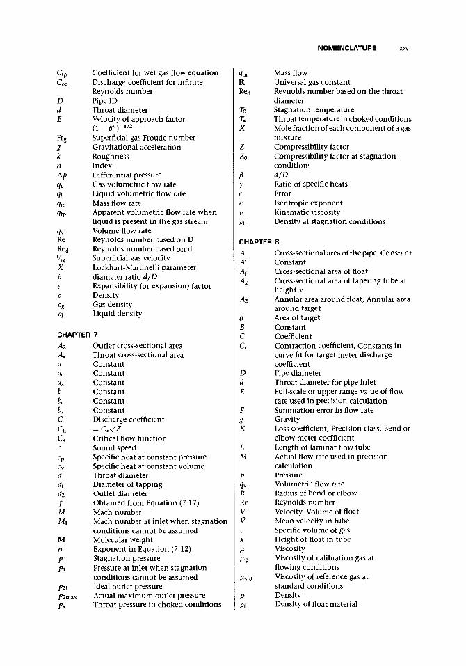
Nomenclature
CHAPTER 1Q Sensitivity coefficientf{x) Function for Normal distributionK K factor in pulses per unit flow quantityk Coverage factorM Mean of a sample of n readingsm IndexN(/JL, a2) Normal curven Number of measurements, Exponentp Probability, Indexq Mean of n measurements qj, Exponentqj Test measurementqv Volumetric flow rateqvo Volumetric flow rate at calibration pointr Exponents Exponents(q) Experimental standard deviation of
mean of group qjs(qj) Experimental standard deviation of qjt Student's tU Expanded uncertaintyu(xi) Standard uncertainty for the zth quantityuc(y) Combined standard uncertaintyx CoordinateXi Result of a meter measurement , Input
quantit iesx Mean of n meter measurementy Output quantityz Normalized coordinate (x — /x)/al± Mean value of data for normal curvev Degrees of freedomo Standard deviation (a2 variance)4>(z) Area under Normal curve [e.g., 4>(0.5) is
the area from z = -oo to z = 0.5]</>(x) Function for normalized Normal
distribution
CHAPTER 2Ac
D
Cross-section of pipeLocal speed of soundSpecific heat at constant pressureSpecific heat at constant volumeDiameter of pipe
d Diameter of tube bundle straightenertubes
g Acceleration due to gravityH Hodgson's numberK Pressure loss coefficientM Mach numbern Index as in Equation (2.4)p Pressurepo Stagnation pressureAPioss Pressure loss across a pipe fittingqv Volumetric flow rateqm Mass flow rateR Radius of pipeRe Reynolds numberr Radial coordinate (distance from pipe
axis)T TemperatureTo Stagnation temperatureV Velocity in pipe, Volume of pipework
and other vessels between the sourceof the pulsat ion and the flowmeterposit ion
Vb Velocity on pipe axisKms Fluctuating component of velocityV Mean velocity in pipez Elevation above datumy Ratio of specific heatsli Dynamic viscosityy Kinematic viscosityp DensitySUBSCRIPTS1,2 Pipe sections
CHAPTER 3Cj Sensitivity coefficient for the zth
quantityfamin Lubrication film thicknessn Bearing rotational speedp Bearing loadui Standard uncertainty for the / th quantityr) Friction coefficientk Specific film thicknessix Fluid viscosity

NOMENCLATURE
a Combined roughness of the twocontacting surfaces of the bearing
CHAPTER 4Q Concentration of tracer in the main
stream at the downstream samplingpoint
Cdmean Mean concentration of tracer measureddownstream during time t
Q Concentration of tracer in the injectedstream
Cu Concentration of tracer in the mainstream upstream of injection point(if the tracer material happens to bepresent)
cx Sensitivity coefficientMn Net mass of liquid collected in
calibrationp Pressureqv Volumetric flow rate in the lineqVi Volumetric flow rate of injected tracerR Gas constant for a particular gasT Temperaturet Collection time during calibration,
Integration period for tracermeasurement
V Amount injected in the sudden injection(integration) method
v Specific volumep Liquid density
CHAPTERAa\
a€bb€CCRe
Claps
c
C\
C*DD1
dE
ET
E*eF
5Function of p and ReExpression in orifice plate bendingformulaConstantConstantConstantDischarge coefficientPart of discharge coefficient affectedby RePart of discharge coefficient whichallows for position of tapsDischarge coefficient for infiniteReynolds numberExpression in orifice plate bendingformulaConstantPipe diameter (ID)Orifice plate support diameterOrifice diameterVelocity of approach factor (1 - £4)~~1/2:,Thickness of the orifice plateTotal error in the indicated flow rate of aflowmeter in pulsating flowElastic modulus of plate materialThickness of the orificeCorrection factors used to obtain themass flow of a (nearly) dry steam flow
fHhK
Li
h
'2
M'2nPdPuAp
qmqvRe
rtV
V
vWs
X
aPyHm
€1
K
Pi
°y
4>
CHAPTER
C
cRe
Frequency of the pulsationHodgson numberThickness of orifice plateLoss coefficient, Related to the criterionfor Hodgson's number= h/D= l'2/D (The prime signifies that themeasurement is from the downstreamface of the plate)Distance of the upstream tappingfrom the upstream face of theplateDistance of the downstream tappingfrom the downstream face of the plate(The prime signifies that themeasurement is from the downstreamface of the plate)= 2L'2/(1 - p)IndexDownstream pressureUpstream pressureDifferential pressure, pressure dropbetween pulsation source and meterMass flow rateVolumetric flow rateReynolds number usually based on thepipe IDRadius of upstream edge of orifice plateTimeVolume of pipework and other vesselsbetween the source of the pulsation andthe flowmeter positionMean velocity in pipe with pulsatingflowRoot-mean-square value of unsteadyvelocity fluctuation in pipe withpulsating flowDryness fractionFlow coefficient, CEDiameter ratio, d/DRatio of specific heatsSmall changes or errors in qm, etc.Expansibility (or expansion) factorExpansibility (or expansion) factor fororificeIsentropic exponentDensity at the upstream pressure tappingcross-sectionYield stress for plate materialRatio of two-phase pressure drop toliquid flow pressure dropMaximum allowable percentage error inpulsating flow
6Coefficient of dischargePart of coefficient of discharge affectedby Reynolds number
NOMENCLATURE
C t p Coefficient for wet gas flow equationCoo Discharge coefficient for infinite
Reynolds numberD Pipe IDd Throat diameterE Velocity of approach factor
(l-/*4)-l/2Frg Superficial gas Froude numberg Gravitational accelerationk Roughnessn IndexAp Differential pressureqg Gas volumetric flow rateqi Liquid volumetric flow rateqm Mass flow rateqtp Apparent volumetric flow rate when
liquid is present in the gas streamqv Volume flow rateRe Reynolds number based on DRed Reynolds number based on dVsg Superficial gas ve loc i tyX Lockhart-Martinelli parameter£ diameter ratio d/De Expansibility (or expansion) factorp Densitypg Gas densityp\ Liquid density
CHAPTER 7A2 Outlet cross-sectional areaA* Throat cross-sectional areaa Constantac Constantaz Constantb Constantbc Constantbz ConstantC Discharge coefficientC R = C*^ZC* Critical flow functionc Sound speedcp Specific heat at constant pressurecv Specific heat at constant volumed Throat diameterdt Diameter of tappingd2 Outlet diameterf Obtained from Equation (7.17)M Mach numberMi Mach number at inlet when stagnation
conditions cannot be assumedM Molecular weightn Exponent in Equation (7.12)po Stagnation pressurepi Pressure at inlet when stagnation
conditions cannot be assumedp2i Ideal outlet pressurep2max Actual maximum outlet pressurep* Throat pressure in choked conditions
RRed
To%X
ZZQ
py
K
V
PO
Mass flowUniversal gas constantReynolds number based on the throatdiameterStagnation temperatureThroat temperature in choked conditionsMole fraction of each component of a gasmixtureCompressibility factorCompressibility factor at stagnationconditionsd/DRatio of specific heatsErrorIsentropic exponentKinematic viscosityDensity at stagnation conditions
CHAPTER 8A Cross-sectional area of the pipe, ConstantA' ConstantAf Cross-sectional area of floatAx Cross-sectional area of tapering tube at
height xA2 Annular area around float, Annular area
around targeta Area of targetB ConstantC CoefficientCc Contraction coefficient, Constants in
curve fit for target meter dischargecoefficient
D Pipe diameterd Throat diameter for pipe inletE Full-scale or upper range value of flow
rate used in precision calculationF Summation error in flow rateg GravityK Loss coefficient, Precision class, Bend or
elbow meter coefficientL Length of laminar flow tubeM Actual flow rate used in precision
calculationp Pressureqv Volumetric flow rateR Radius of bend or elbowRe Reynolds numberV Velocity, Volume of floatV Mean velocity in tubev Specific volume of gasx Height of float in tube/x Viscosityfig Viscosity of calibration gas at
flowing conditions/xstd Viscosity of reference gas at
standard conditionsp DensityPi Density of float material

NOMENCLATURE
CHAPTER 9E Young's modulus of elasticityF Friction forceg Acceleration due to gravityL Length of clearance gap in direction
of flowI Axial length of clearance gap£ax Axial length of measuring chamberM Mass of rotorN Rotational speed of rotorN[ Rotational speed of cam disk of calibrator
(clutch system)NIN Rotational speed of shaft into calibrator
(epicyclic system)Nmax Max imum rotational speed of rotorNo Rotational speed of outer ring of
calibrator (clutch system)NOUT Rotational speed of shaft out of
calibrator (epicyclic system)Ns Slippage in NINn Number of teeth on gearpa Downstream pressurep u Upstream pressure<Zideai A s u s e d i n Equation (9.A.6)leakage Leakage flow rate<?BULK Bulk volumetric flow rate<7siip Volumetric flow rate through meter at no
rotationqv Volumetric flow rateR Radius of friction wheelr Radius of point of friction wheel
contactrx Inner radius of measuring chamberro Outer radius of measuring chamberrs Shaft radiusT Temperature, TorqueTIN Torque on input shaft to calibratorTOUT Torque out from calibrator7b Constant drag torqueT\ Speed-dependent drag torquet Clearance between stationary and
moving memberst0 Thickness of outer casingu Fluid velocityy Position coordinate across clearance gapam Coefficient of linear expansion of metal«i Coefficient of volume expansion of
liquidA Change in quantity, Distance between
center of rotation of arm and center ofdiscs in calibrator
8 Reduction in area of the measuringchamber due to blade sections
9Q Angular position of center disk ofcalibrator
0[ Angular position of cam disk of calibrator0o Angular position of outer ring of
calibrator
ViscosityAngular position of arm of calibrator
OTHER/1m1,21-8
SUBSCRIPTSDummy suffix for summationLiquidMetalDifferent materialsEpicyclic gears
CHAPTER 1 0A
a
do, U\,#2/ #3Bb
C
cDcD
ctch
CLcD
D\D2
£>3d\, d2eFfI
ii(r)K
K(r)Ki,K2
Kh
LNnPpoiP02
Cross-sectional area of the effectiveannular flow passage at the rotor bladesTurbine meter aerodynamic torquecoefficient
Constant coefficientsAxial length of rotorTurbine meter aerodynamic torquecoefficient, Bearing length, Frequencyresponse coefficient unless used as anexponentProportional to 1/KDrag coefficientDrag coefficient adjusted to allowforChFluid drag coefficientConstant for a particular design (Behaveslike an adjustment to the mainaerodynamic drag term coefficient)Lift coefficientChordDrag force, Pipe diameter, ImpellerdiameterRotor response parameterFluid drag parameterNonfluid drag parameterAdditional geometric variablesMeter errorNonfluid forcesFrequency of blade passingMass moment of inertia of rotor systemabout rotor axisIncidence angleIncidence at radius rLattice effect coefficient, K factor(pulses/unit volume)Lattice coefficient at radius rTurbine meter resisting torquecoefficientsConstant used in equation for helicalblade angleLift force, Helical pitch of bladesNumber of bladesRotational speed (frequency)Index in error equationStagnation pressure at inletStagnation pressure at outlet

NOMENCLATURE
pi Static pressure at inletp2 Static pressure at outletq Actual average flow rate, Index in error
equationqo Time average flow rate over period Tq\ Initial flow rateqi Final flow rateqb Base flow rateq\ Indicated average flow rate<?max Maximum flow rate for which the meter
is designed<7min Minimum flow rate for which the meter
is designedqn Normal flow rateqt Flow rate at time ttrans Flow rate at change of precision
qv Volumetric flow rateR Pipe bend radiusRe Reynolds numberr Radial position, Index in error
equationrj Journal bearing radiusrh Hub radiusro Meter bore radiusrt Tip radiusS Slope of no-flow decay curve at
standstills Blade spacingT Temperature, Fundamental period of
pulsating flow, TorqueTB Bearing drag torqueTc Tempera ture at cal ibrat ionTd Driving to rqueTpo Mechanical friction torque on rotor at
zero speedTh Hub fluid drag torqueTn Nonfluid drag torque7^> Temperature at operat ionTr Retarding torqueTt Blade t ip clearance drag torqueT w Hub disk friction drag torquet Time£B Blade thickness£R Relaxation t imeV N o n d i m e n s i o n a l fluid velocityVo Time average value of Vz over per iod TV\ Inlet relative flow velocityV2 Out le t relative flow velocity^rnax M a x i m u m value of Vz
^rnin M i n i m u m value of Vz
Vz Axial velocity (instantaneous inlet fluidvelocity of pulsating flow)
W Rotor blade velocity, Nondimensionalinstantaneous rotor velocity underpulsating flow
Wh Relative velocity at the hubY Tangential forceZ Axial force
a
Pip2Pmr8
nV
pX
CHAPTER
A
aB
DfHh
K
L
A/7
PatmosPgmin
PvqvReSs
VVmaxW
8Q
CO
Wave shape coefficient, Thermalcoefficient of expansion, Angle betweeninlet flow direction and far field flowBlade angle at radius r measured fromaxial direction of meterRelative inlet angle of flowRelative outlet angle of flowMean of the inlet and outlet flow fieldFull-flow amplitude relative to averageflowDeflection of flow at blade outlet fromblade angleFlow deviation factorDynamic viscosityKinematic viscosityFluid densityNondimensional time (t/T), Period ofmodulationRotor coast time to standstillInstantaneous rotor angular velocity
11Pipe full flow area, Constant of valueabout 3.0 used in equation for avoidingcavitation in flows past vortex metersFlow area past bluff bodyArea when integrating vorticityConstant of value about 1.3 used inequation for avoiding cavitation in flowspast vortex metersPipe IDShedding frequencyStreamwise length of bluff bodyParallel flats on sides of bluff body atleading edgeCalculation factor for sheddingfrequency (Zanker and Cousins 1975),K factor = pulses/unit volumeLength of bluff body across pipe betweenend fittingsPressure drop across vortex meter(about 1 bar at 10 m/s)Atmospheric pressureMinimum back pressure 5D downstreamof vortex meterSaturated liquid vapor pressureVolumetric flow rateReynolds numberStrouhal numberLength along curve when integratingvelocity around a vortexVelocity of flowVelocity of flow past bluff bodyDiameter or width of bluff bodyShear layer thicknessInjected swirling flow rate/total flowrateVorticity

NOMENCLATURE
CHAPTER 12A Used for area of electrode leads forming
a loop causing quadrature signals in theelectromagnetic flowmeter
a Pipe radiusB Magnetic flux density in teslaB Magnetic flux density vectorBo Maximum value of magnetic flux
densityBe 6 component of magnetic flux densityb Inner radius of an annulus of conducting
fluid in two phase annular flowD Diameter of pipeE Electric field vectorf Frequency of magnetic field excitationj Current density vector/ Length of wire traversing magnetic fieldAp Pressure of the pipeline fluid above
atmosphericqv Volumetric flow rater Radial coordinate5 Electromagnetic flowmeter sensitivityt Pipe wall thicknessU Electric potentialAI/EE Voltage between electrodesAC/p Voltage across a wire P moving through
a magnetic field (similarly for Q and R)V VelocityV Velocity vectorVm Mean velocity in the pipe in meters per
secondW Weighting functionW Weight function vectorW Rectilinear flow weight functionW" Axisymmetric weight functionWz Axial component of Wa Void fraction€ Strain6 Cylindrical coordinate\x Electric permeabilitya Conductivity<t> Scalar potential
CHAPTERA
ac
Df
/d
ftfr/u
13Weighting factors for GaussianquadratureRadius of pipeVelocity of ultrasound in the medium,Coefficients of a polynomialPipe diameterFrequency of stable quartz oscillator forultrasonic measurement systemFrequency for the downstreamsing-around pulse trainTransmitted doppler frequencyReflected doppler frequencyFrequency for the upstream sing-aroundpulse train
y
zz
(37eXpPmT
xm
fit)
h
I
L
PRPI
ReRyxir)Tt
tm
At
VVm
V(X)V5
VoV
WX
Difference between the sing-aroundfrequencies, Frequency shift in dopplerflowmeterFunction of tDisplacement of ultrasonic beam fromaxis of pipeDriving current in ultrasonic flowmeterAdiabatic compressibilityDistance along path in transit-timeflowmeter, Distance between transducersin ultrasonic correlation flowmeterCounters for ultrasonic measuringsystem\/n is the index for turbulent profilecurve fit, IndexUltrasound power reflectedUltrasound power transmittedMass flow rateReynolds numberCorrelation coefficientCorrelation time for integrationPipe wall thicknessDownstream wave transit timeMean wave transit timeUpstream wave transit timeDifference between these two wavetransit timesBeam positions for ultrasonic flowmeterusing Gaussian quadratureReceived voltages for ultrasonicflowmeterFlow velocity in pipeMean velocity in pipeFlow velocity profile along pipe chordUltrasonic flowmeter created flowAcoustic field for cases (1) and (2)Relative flow velocity in the direction ofthe acoustic beamVector weight functionAxial length between transducers inultrasonic flowmeterLength of chord in the plane of theultrasonic pathDistance along chord used in ultrasonicflowmeterAcoustic impedanceUltrasonic beam deflection distance onopposite wallUltrasonic beam deflection angleRatio of specific heats for a particular gasUltrasound beam angleUltrasound wave lengthDensity of materialMean density in ultrasonic meterMeasurement period for ultrasonicsystem, Time period betweenultrasonic wave peaksMean ultrasonic correlation time
NOMENCLATURE
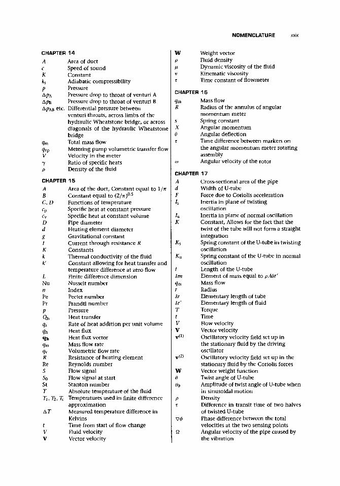
CHAPTER 14A Area of ductc Speed of soundK Constantks Adiabatic compressibilityp PressureA/?A Pressure drop to throat of venturi AA/?B Pressure drop to throat of venturi BApAB etc. Differential pressure between
venturi throats, across limbs of thehydraulic Wheatstone bridge, or acrossdiagonals of the hydraulic Wheatstonebridge
qm Total mass flowqvp Metering pump volumetric transfer flowV Velocity in the meter7 Ratio of specific heatsf> Density of the fluid
CHAPTER 15ABC,D
Area of the duct, Constant equal to 1/nConstant equal to (2/TT)0-5
Functions of temperaturecp Specific heat at constant pressurecv Specific heat at constant volumeD Pipe diameterd Heating element diameterg Gravitational constant/ Current through resistance RK Constantsk Thermal conductivity of the fluidkf Constant allowing for heat transfer and
temperature difference at zero flowI Finite difference dimensionNu Nusselt numbern IndexPe Peclet numberPr Prandtl numberp PressureQ h Heat transfer<ja Rate of heat addition per unit volumeq\y Heat fluxq h Heat flux vectorqm Mass flow rateqv Volumetric flow rateR Resistance of heating elementRe Reynolds number5 Flow signalSo Flow signal at startSt Stanton numberT Absolute temperature of the fluidTi,Tz,Tc Temperatures used in finite difference
approximationAT Measured temperature difference in
Kelvinst Time from start of flow changeV Fluid velocityV Vector velocity
W Weight vectorp Fluid density[i Dynamic viscosity of the fluidv Kinematic viscosityT Time constant of flowmeter
CHAPTER 16qm Mass flowR Radius of the annulus of angular
momentum meters Spring constantX Angular momentum0 Angular deflectionT Time difference between markers on
the angular momentum meter rotatingassembly
co Angular velocity of the rotor
CHAPTERAdFh
/uK
Ks
Ku
I8mqmr8r8r'TtVVv(!)
v(2)
w0
pX
Q
17Cross-sectional area of the pipeWidth of U-tubeForce due to Coriolis accelerationInertia in plane of twistingoscillationInertia in plane of normal oscillationConstant, Allows for the fact that thetwist of the tube will not form a straightintegrationSpring constant of the U-tube in twistingoscillationSpring constant of the U-tube in normaloscillationLength of the U-tubeElement of mass equal to pA8r'Mass flowRadiusElementary length of tubeElementary length of fluidTorqueTimeFlow velocityVector velocityOscillatory velocity field set up inthe stationary fluid by the drivingoscillatorOscillatory velocity field set up in thestationary fluid by the Coriolis forcesVector weight functionTwist angle of U-tubeAmplitude of twist angle of U-tube whenin sinusoidal motionDensityDifference in transit time of two halvesof twisted U-tubePhase difference between the totalvelocities at the two sensing pointsAngular velocity of the pipe caused bythe vibration

NOMENCLATURE
CO
cos
COu
CHAPTER
Amplitude of the angular velocity of thepipe caused by the vibrationDriving frequencyNatural frequency of U-tube in twistingoscillationNatural frequency of U-tube in normaloscillation
18
AAtAninAx
A2
A*a
k CoefficientM Mach numberp Pressurep0 Stagnation pressureAp Dynamic pressureV Velocityy Ratio of specific heatsp Density
CHAPTER 20C Costcp Component precisionD Pipe diameterd Width of Coriolis flowmeter U-tubeeq Electronics qualityK ConstantKs Spring constant of the U-tube in twisting
oscillationma Manufacturing accuracyme Material consistencyPi, pi,p3, p4 Dimensional and other factorsqm Mass flow rateqw Volumet r i c flow rate5 Flow signalAt Time difference between upstream and
downstream waves or pulsestm Mean time of transit used to obtain
sound speed0 Ultrasound beam angler Difference in transit time of two halves
of twisted U-tubeco Driving frequencycos Natural frequency of U-tube in
twisting oscillation
COMBINED ALL CHAPTERSA Cross-section of pipe, Function of p and
Re, Cross-sectional area of the pipe,Constant, Cross-sectional area of theeffective annular flow passage at therotor blades, Constant of value about 3.0used in equation for avoiding cavitationin flows past vortex meters, Used for areaof electrode leads forming a loopcausing quadrature signals in theelectromagnetic flowmeter, Weightingfactors for Gaussian quadrature, Area ofthe duct, Constant equal to 1 In
0, 01/
ac
BBo
bz
hC
CD
Qmean
Q
Q
CL
CR
ConstantCross-sectional area of floatFlow area past bluff bodyCross-sectional area of tapering tubeat height xOutlet cross-sectional area, Annular areaaround float, Annular area around targetThroat cross-sectional areaConstant, Area of target, Turbinemeter aerodynamic torque coefficient,Area when integrating vorticity, Piperadius
Constant coefficientsExpression in orifice plate bendingformulaConstantConstantConstantConstant, Axial length of rotor, Constantof value about 1.3 used in equation foravoiding cavitation in flows past vortexmeters, Magnetic flux density in tesla,Constant equal to (2/TT)0-5
Magnetic flux density vectorMaximum value of magnetic fluxdensity0 component of magnetic flux densityInner radius of an annulus of conductingfluid in two-phase annular flowConstant, Turbine meter aerodynamictorque coefficient, Bearing length,Frequency response coefficient unlessused as an exponentConstantConstantConstantDischarge coefficient, Coefficient,Proportional to 1/K, Function oftemperature, CostContraction coefficient, Constants incurve fit for target meter dischargecoefficientDrag coefficientDrag coefficient adjusted to allow for Ch
Concentration of tracer in the mainstream at the downstream samplingpointMean concentration of tracer measureddownstream during time tFluid drag coefficientConstant for a particular design (Behaveslike an adjustment to the mainaerodynamic drag term coefficient)Concentration of tracer in the injectedstreamLift coefficient

NOMENCLATURE
CRe Part of discharge coefficient affected by ReCraps P a r t °f discharge coefficient tha t allows
for posit ion of tapsQp Coefficient for wet gas flow equat ionCu Concent ra t ion of tracer in the main
stream upstream of injection poin t (if thetracer material happens to be present)
Coo Discharge coefficient for infiniteReynolds number
C* Critical flow functionc Sound/ul t rasound speed, Chord,
Coefficients of a polynomialc\ Expression in orifice plate bending
formulaQ Sensitivity coefficientcp Specific heat at constant pressurecp C o m p o n e n t precisioncv Specific heat at constant volumec€ ConstantD Pipe diameter (ID), Drag force, Impeller
diameter, Function of temperatureD' Orifice plate support diameterD\ Rotor response parameterD2 Fluid drag parameterD3 Nonfluid drag parameterd Diameter of tube bundle straightener
tubes, Orifice diameter, Throat diameter,Heating element diameter, Width ofCoriolis flowmeter U-tube
dt Diameter of tappingd\ Additional geometric variabledz Outlet diameter, Additional geometric
variableE velocity of approach factor (1 - £4)~1 /2 ,
Thickness of the orifice plate, Full-scaleor upper range value of flow rate used inprecision calculation, Young's modulusof elasticity, Fluid compressibility
E Electric field vectorEj Total error in the indicated flow rate of a
flowmeter in pulsating flowE* Elastic modulus of plate materiale Thickness of the orifice, Meter erroreq Electronics qualityF Correction factors used to obtain the
mass flow of a (nearly) dry steam flow,Summation error in flow rate, Frictionforce, Nonfluid forces, Force due toCoriolis acceleration
Frg Superficial gas Froude numberf Frequency of the pulsation, Obtained
from Equation (7.17), Frequency of bladepassing, Shedding frequency, Frequencyof magnetic field excitation, Frequencyof stable quartz oscillator for ultrasonicmeasurement system
fy Frequency for the downstreamsing-around pulse train
ft Transmitted doppler frequencyft Reflected doppler frequencyfu Frequency for the upstream sing-around
pulse trainA f Difference between the sing-around
frequencies, Frequency shift in dopplerflowmeter
f{t) Function of tfix) Function for Normal distributiong Acceleration due to gravityH Hodgson number, Streamwise length of
bluff bodyh Thickness of orifice plate, Parallel flats on
sides of bluff body at leading edge,Displacement of ultrasonic beam fromaxis of pipe
frmin Lubrication film thickness/ Mass moment of inertia of rotor system
about rotor axis, Driving current inultrasonic flowmeter, Current throughresistance R
Is Inertia in plane of twisting oscillationJu Inertia in plane of normal oscillationi Incidence angle/(r) Incidence at radius rj Current density vectorK Pressure loss coefficient, Related to the
criterion for Hodgson's number,Precision class, Bend or elbow metercoefficient, Lattice effect coefficient, Kfactor (pulses/unit volume), Calculationfactor for shedding frequency (Zankerand Cousins 1975), Constant, Allows forthe fact that the twist of the tube will notform a straight integration
Kir) Lattice coefficient at radius rK\,Ki Turbine meter resisting torque
coefficientsKh Constant used in equation for helical
blade angleKs Spring constant of the U-tube in twisting
oscillationKu Spring constant of the U-tube in normal
oscillationk Coverage factor, Roughness, Thermal
conductivity of the fluid, Coefficientk! Constant allowing for heat transfer and
temperature difference at zero flowks Adiabatic compressibilityL Length of laminar flow tube, Length of
clearance gap in direction of flow, Liftforce, Helical pitch of blades, Length ofbluff body across pipe between endfittings, Distance along path intransit-time flowmeter, Distancebetween transducers in ultrasoniccorrelation flowmeter, Finite differencedimension

NOMENCLATURE
L'2
V2
I
M
MMi
M2
Mn
m8mmameN
Ns
Nd,NnNt,NuN(/JL, a2)Nu
PRPrPePrPatmos
h/DV2/D (The prime signifies that themeasurement is from the downstreamface of the plate)Length of wire traversing magnetic field,Length of the U-tubeDistance of the upstream tapping fromthe upstream face of the plateDistance of the downstream tappingfrom the downstream face of the plate(The prime signifies that themeasurement is from the downstreamface of the plate)Axial length of clearance gapAxial length of measuring chamberMean of a sample of n readings, Machnumber, Actual flow rate used inprecision calculation, Mass of rotorMolecular weightMach number at inlet when stagnationconditions cannot be assumed= 2L'2/(1 - P)Net mass of liquid collected incalibrationIndexElement of mass equal to pASr'Manufacturing accuracyMaterial consistencyRotational speed of rotor, Number ofbladesRotational speed of cam disk of calibrator(clutch system)Rotational speed of shaft into calibrator(epicyclic system)Maximum rotational speed of rotorRotational speed of outer ring ofcalibrator (clutch system)Rotational speed of shaft out of calibrator(epicyclic system)Slippage in N|NCounters for ultrasonic measuringsystemNormal curveNusselt numberNumber of measurements, Exponentin equations, Bearing rotational speed,Number of teeth on gear, Rotationalspeed (frequency)Probability, Pressure, Bearing load,Exponent in error equationUltrasound power reflectedUltrasound power transmittedPeclet numberPrandtl numberAtmospheric pressureDownstream pressureMinimum back pressure 5D downstreamof vortex meter
PoPuPvPoiP02Pi
P2P2iP2maxP*
ApBApAB etc
ApiossAp
Qhq
qqoq\qiq*
<?BULKqgqhq h
<?idealqi
q\qi^leakageqmqmax
qmin
qn
qtp
^trans^slip
qv
Stagnation pressureUpstream pressureSaturated liquid vapor pressureStagnation pressure at inletStagnation pressure at outletPressure at inlet when stagnationconditions cannot be assumed, Staticpressure at inlet, p\pi dimensional andother factorsStatic pressure at outletIdeal outlet pressureActual maximum outlet pressureThroat pressure in choked conditionsPressure drop to throat of venturi APressure drop to throat of venturi B
. Differential pressure betweenventuri throats, across limbs of thehydraulic Wheatstone bridge, or acrossdiagonals of the hydraulic WheatstonebridgePressure loss across a pipe fittingDifferential pressure, Pressure dropbetween pulsation source and meter,Pressure drop across vortex meter(about 1 bar at 10 m/s), Pressure of thepipeline fluid above atmospheric,Dynamic pressureHeat transferActual average flow rate; Exponent inerror equationMean of n measurements q\Time average flow rate over period TInitial flow rateFinal flow rateRate of heat addition per unit volumeBase flow rateBulk volumetric flow rateGas volumetric flow rateHeat fluxHeat flux vectorAs used in Equation (9.A.6)Indicated average flow rateTest measurementLiquid volumetric flow rateLeakage flow rateMass flow rateMaximum flow rate for which the meteris designedMinimum flow rate for which the meteris designedNormal flow rateFlow rate at time tApparent volumetric flow rate whenliquid is present in the gas streamFlow rate at change of precisionVolumetric flow rate through meter at norotationVolumetric flow rate (in the main line)

NOMENCLATURE
<?vo<7vP
qv\R
RRe
Red
Ryx(r)r
nr)ro
rs8r8r'S
SoSt5
s(q)
s(q\)T
7BTc
Td
TFO
Th
TINTn
TOUT
To
Tr
Tt
TW7i
Volumetric flow rate at calibration pointMetering pump volumetric transferflowVolumetric flow rate of injected tracerRadius of pipe, Gas constant for aparticular gas, Radius of bend or elbow,Radius of friction wheel, Resistance ofheating element, Radius of the annulusof angular momentum meterUniversal gas constantReynolds number usually based on thepipe IDReynolds number based on the throatdiameterCorrelation coefficientRadial coordinate (distance from pipeaxis), Radius of upstream edge of orificeplate, Radius of point of friction wheelcontact, Exponent, RadiusHub radiusInner radius of measuring chamberJournal bearing radiusTip radiusOuter radius of measuring chamber,Meter bore radiusShaft radiusElementary length of tubeElementary length of fluidSlope of no-flow decay curve atstandstill, Strouhal number,Electromagnetic flowmeter sensitivity,Flow signalFlow signal at startStanton numberExponent, Experimental standarddeviation, Blade spacing, Length alongcurve when integrating velocity arounda vortex, Spring constantExperimental standard deviation ofmean of group q^Experimental standard deviation of q^Temperature, Torque, Fundamentalperiod of pulsating flowBearing drag torqueTemperature at calibrationDriving torqueMechanical friction torque on rotor atzero speedHub fluid drag torqueTorque on input shaft to calibratorNonfluid drag torqueTorque out from calibratorStagnation temperature, Constant dragtorque, Temperature at operationRetarding torqueBlade tip clearance drag torqueHub disk friction drag torqueSpeed-dependent drag torque
Ti,T2,Tc
T*
AT
t
£Btdtm
to£RtuAt
t\,t2
U
AC/EEAC/p
My)V
V
*4ms
Vv(l)
v(2)
vm
nnax
^min
vsV o
vz
Temperatures used in finite differenceapproximationThroat temperature in chokedconditionsMeasured temperature difference inKelvinsStudent's t, Collection time duringcalibration, Integration period fortracer measurement, Time, Clearancebetween stationary and movingmembers, Pipe wall thicknessBlade thicknessDownstream wave timeMean time of transit used to obtainsound speedThickness of outer casingRelaxation timeUpstream wave timeTime difference between upstream anddownstream waves or pulsesBeam positions for ultrasonic flowmeterusing Gaussian quadratureExpanded uncertainty, ElectricpotentialVoltage between electrodesVoltage across a wire P moving througha magnetic field (similarly for Q and R)Received voltages for ultrasonicflowmeterStandard uncertainty for the /th quantityCombined standard uncertaintyFluid velocity, Amount injected in thesudden injection (integration) method,Volume of pipework and other vesselsbetween the source of the pulsation andthe flowmeter position, Volume of float,Nondimensional fluid velocityMean velocity in pipe with pulsatingflowRoot-mean-square value of unsteadyvelocity fluctuation in pipe withpulsating flowVelocity vectorOscillatory velocity field set up in thestationary fluid by the driving oscillatorOscillatory velocity field set up in thestationary fluid by the Coriolis forcesMean velocity in the pipe in meters persecondMaximum value of Vz, Velocity of flowpast bluff bodyMinimum value of VzVelocity on pipe axisUltrasonic undisturbed flowAcoustic field for cases (1) and (2)Superficial gas velocityAxial velocity (instantaneous inlet fluidvelocity of pulsating flow)

NOMENCLATURE
Vo Time average value of Vz over per iod TV\ In le t re la t ive flow ve loc i tyVz Outlet relative flow velocityV Mean velocity in pipev Specific volume of gas, Relative flow
velocity in the direction of the acousticbeam
W Rotor blade velocity, Nondimensionalinstantaneous rotor velocity underpulsating flow, Weighting function
W Weight function vectorW Rectilinear flow weight functionW" Axisymmetric weight functionW\i Relative velocity at the hubWz Axial component of Ww Diameter or width of bluff bodyX Axial length between transducers in
ultrasonic flowmeter, Mole fraction ofeach component of a gas mixture,Angular momentum, Lockhart-Martinelli parameter
x Coordinate, Dryness fraction, Height offloat in tube
Xi Result of a meter measurementx Mean of n meter measurementsY Length of chord in the plane of the
ultrasonic path, Tangential forcey Output quantity, Wetness fraction,
Position coordinate across clearance gap,Distance along chord used in ultrasonicflowmeter
Z Compressibility factor, Axial force,Acoustic impedance
Zo Compressibility factor at stagnationconditions
z Normalized coordinate (x — ii)/o,Elevation above datum, Ultrasonic beamdeflection distance on opposite wall
a Flow coefficient CE, Wave shapecoefficient, Thermal coefficient of expan-sion, Angle between inlet flow directionand far field flow, Void fraction
am Coefficient of linear expansion of metala\ Coefficient of volume expansion of
liquid0 Diameter ratio d/D, Blade angle at radius
r measured from axial direction of meter,Ultrasonic beam deflection angle
01 Relative inlet angle of flow02 Relative outlet angle of flow0m Mean of the inlet and outlet flow fieldy Ratio of specific heatsr Full-flow amplitude relative to average
flowA Change in quantity, Distance between
center of rotation of arm and center ofdiscs in calibrator
8qm etc.
fig
pPipm
poo
r
rm
Reduction in area of the measuringchamber due to blade sections,Deflection of flow at blade outletfrom blade angle, Shear layerthicknessSmall changes or errors in qm, etc.Expansibility (or expansion) factor,Error, StrainExpansibility (or expansion) factor fororificeFriction coefficient, Flow deviationfactorCylindrical coordinate, Ultrasoundbeam angle, Angular deflection, Twistangle of U-tubeAngular position of center disk ofcalibratorAngular position of cam disk of calibratorAngular position of outer ring ofcalibrator, Amplitude of twist angle ofU-tube when in sinusoidal motionIsentropic exponentSpecific film thickness, Ultrasound wavelengthMean value of data for normal curve,Dynamic viscosity, Fluid viscosity,Electric permeabilityViscosity of calibration gas at flowingconditionsViscosity of reference gas at standardconditionsDegrees of freedom, KinematicviscosityDensity, Fluid densityDensity of float materialMean density in ultrasonic meterDensity at stagnation conditionsStandard deviation (a2 variance),Combined roughness of the twocontacting surfaces of the bearing,ConductivityYield stress for plate materialNondimensional time (t/T), Period ofmodulation, Measurement period forultrasonic system, Time period betweenultrasonic wave peaks, Time constantof flowmeter, Time difference betweenmarkers on the angular momentummeter rotating assembly, Difference intransit time of two halves of twistedU-tubeMean ultrasonic correlation timeRotor coast time to standstillAngular position of arm of calibrator,Scalar magnetic potentialArea under Normal curve [e.g., 0(0.5) isthe area from z= - oo to z = 0.5]

NOMENCLATURE
Q
Ratio of two-phase pressure drop toliquid flow pressure dropMaximum allowable percentage error inpulsating flowFunction for normalized NormaldistributionPhase difference between the totalvelocities at the two sensing pointsInjected swirling flow rate/total flow rate,Angular velocity of the pipe caused bythe vibrationAmplitude of the angular velocity of thepipe caused by the vibration insinusoidal motion
CO
cos
cou
OTHER
//m1,21-8
Instantaneous rotor angular velocity,Vorticity, Angular velocity of the rotor,Driving frequencyNatural frequency of U-tube in twistingoscillationNatural frequency of U-tube in normaloscillation
SUBSCRIPTSDummy suffix for summationLiquidMetalPipe sections, Different materialsEpicyclic gears


CHAPTER
Introduction
1.1 INITIAL CONSIDERATIONS
Some years ago at Cranfield, where we had set up a flow rig for testing the effectof upstream pipe fittings on certain flowmeters, a group of senior Frenchmen werebeing shown around and visited this rig. The leader of the French party recalled asimilar occasion in France when visiting such a rig. The story goes something likethis.
A bucket at the end of a pipe seemed particularly out of keeping with the remain-ing high tech rig. When someone questioned the bucket's function, it was explainedthat the bucket was used to measure the flow rate. Not to give the wrong impressionin the future, the bucket was exchanged for a shiny new high tech flowmeter. In duecourse, another party visited the rig and observed the flowmeter with approval. "Andhow do you calibrate the flowmeter?" one visitor asked. The engineer responsiblefor the rig then produced the old bucket!
This book sets out to guide those who need to make decisions about whetherto use a shiny flowmeter, an old bucket, nothing at all, or a combination of these!It also provides information for those whose business is the design, manufacture,or marketing of flowmeters. I hope it will, therefore, be of value to a wide varietyof people, both in industry and in the science base, who range across the wholespectrum from research and development through manufacturing and marketing.In my earlier book on flow measurement (Baker 1988/9), I provided a brief statementon each flowmeter to help the uninitiated. This book attempts to give a much morethorough review of published literature and industrial practice.
This first chapter covers various general points that do not fit comfortably else-where. In particular, it reviews recent guidance on the accuracy of flowmeters (orcalibration facilities).
The second chapter reviews briefly some essentials of fluid mechanics necessaryfor reading this book. The reader will find a fuller treatment in Baker (1996), whichalso has a list of books for further reading.
A discussion of how to select a flowmeter is attempted in Chapter 3, and someindication of the variety of calibration methods is given in Chapter 4, before goingin detail in Chapters 5-17 into the various high (and low) tech meters available.Chapter 18 deals with probes, Chapter 19 gives a brief note on modern controlsystems, and Chapter 20 provides some reflections on manufacturing and markets.Finally, Chapter 21 raises some of the interesting directions in which the technologyis likely to go in the future.

INTRODUCTION
In this book, I have tried to give a balance between the laboratory ideal, themanufacturer's claims, the realities of field experience, and the theory behind thepractice. I am very conscious that the development and calibration laboratories aresometimes misleading places, which omit the problems encountered in the field(Stobie 1993), and particularly so when that field happens to be the North Sea. Inthe same North Sea Flow Measurement Workshop, there was an example of the un-expected problems encountered in precise flow measurement (Kleppe and Danielsen1993), resulting, in this case, from a new well being brought into operation. It hadsignificant amounts of barium and strontium ions, which reacted with sulfate ionsfrom injection water and caused a deposit of sulfates from the barium sulfate andstrontium sulfate that were formed.
With that salutary reminder of the real world, we ask an important - and perhapsunexpected - question.
1.2 DO WE NEED A FLOWMETER?
Starting with this question is useful. It may seem obvious that anyone who looks tothis book for advice on selection is in need of a flowmeter, but for the process engi-neer it is an essential question to ask. Many flowmeters and other instruments havebeen installed without careful consideration being given to this question and with-out the necessary actions to ensure proper documentation, maintenance, and cali-bration scheduling being taken. They are now useless to the plant operator and mayeven be dangerous components in the plant. Thus before a flowmeter is installed,it is important to ask whether the meter is needed, whether there are proper main-tenance schedules in place, whether the flowmeter will be regularly calibrated, andwhether the company has allocated to such an installation the funds needed toachieve this ongoing care. Such care will need proper documentation.
The water industry in the United Kingdom has provided examples of the prob-lems associated with unmaintained instruments. Most of us who are involved inthe metering business will have sad stories of the incorrect installation or misuseof meters. Reliability-centered maintenance recognizes that the inherent reliabilitydepends on the design and manufacture of an item, and if necessary this will needimproving (Dixey 1993). It also recognizes that reliability is preferable in criticalsituations to extremely sophisticated designs, and it uses failure patterns to selectpreventive maintenance.
In some research into water consumption and loss in urban areas, Hopkins et al.(1995) found that obstacles to accurate measurements were
• buried control valves,• malfunctioning valves,• valve gland leakage,• hidden meters that could not be read, and• locked premises denying access to meters.
They commented that "water supply systems are dynamic functions having tobe constantly expanded or amended. Consequently continuous monitoring, revi-sions and amendments of networks records is imperative. Furthermore, a proper

1.2 DO WE NEED A FLOWMETER?
programme of inspection, maintenance and subsequent recording must be opera-tive in respect of inter alia:
• networks,• meters,• control valves,• air valves,• pressure reducing valves,• non-return valves."
They also commented on the poor upstream pipework at the installation of manydomestic meters.
So I make no apology for emphasizing the need to assess whether a flowmeter isactually needed in any specific application.
If the answer is yes, then there is a need to consider the type of flowmeter andwhether the meter should be measuring volume or mass. In most cases, the mostlogical measure is mass. However, by tradition and industrial usage, there are placeswhere volume measurement may be the norm, and as a result, the regulations havebeen written for volume measurement. This results in a Catch-22 situation. The in-dustry and the regulations may, reasonably, resist change to mass flow measurementuntil there is sufficient industrial experience, but industrial experience is not pos-sible until the industry and the regulations allow. The way forward is for one ormore forward-looking companies to try out the new technology and obtain fieldexperience, confidence in the technology, and approval.
In this book, I have made no attempt to alert the reader to the industry-specificregulations and legal requirements, although some are mentioned. Some regulationsare touched on by the various authors, and Miller (1996) is a source of informa-tion on many documents. The main objective of the Organisation Internationalde Metrologie Legale (OIML) is to prevent any technical barriers to internationaltrade resulting from conflicting regulations for measuring instruments. With regardto flow measurement, it is particularly concerned with the measurement of domes-tic supplies and industrial supplies of water and gas (Athane 1994). This is becausethere are two parties involved, the supplier and the consumer, and the consumeris unlikely to be able to ascertain the correct operation of the meter. In additionthese measurements are not monitored continually by the supplier, the meters mayfail without anyone knowing, the usage is irregular and widely varying in rate, themeasurements are not repeatable, and the commodities have increased in value con-siderably in recent years.
In order to reduce discussions and interpretation problems between manufactur-ers and authorized certifying institutes, the European Commission is mandating theEuropean standardization body (CEN/CENELEC) to develop harmonized standardsthat will give the technical details and implementation of the requirements basedon OIML recommendations. These are such that a measuring instrument complieswith essential requirements, assuming that the manufacturer has complied withthem (Nederlof 1994).
The manufacturer will also be fully aware of the electromagnetic compatibil-ity (EMC), which relates to electromagnetic interference. In particular, the EMC

INTRODUCTION
characteristics of a product are that
• the level of electromagnetic disturbance generated by the instrument will notinterfere with other apparatus, and
• the operation of the instrument will not be adversely affected by electromagneticinterference from its environment.
In order to facilitate free movement within the European area the CE mark identifiesproducts that conform to the European essential requirements, and all products mustbe so marked within the European Economic Area (DTI 1993, Chambers 1994).
First, we consider the knotty problem of how accurate the meter should be.
1.3 HOW ACCURATE?
There continues to be inconsistency about the use of terms that relate to accuracyand precision. This stems from a slight mismatch between the commonly used termsand those that the purists and the standards use. Thus we commonly refer to anaccurate measurement, when strictly we should refer to one with a small value ofuncertainty. We should reserve the use of the word accurate to refer to the instrument.A high quality flowmeter, carefully produced with a design and construction totight tolerances and with high quality materials as well as low wear and fatiguecharacteristics, is a precise meter with a quantifiable value of repeatability. Also, itwill, with calibration on an accredited facility, be an accurate meter with a smalland quantifiable value of measurement uncertainty. In the context of flowmeters,the word repeatability is preferred to reproducibility. The meanings are elaborated onlater, and I regret the limited meaning now given to precision, which I have usedmore generally in the past and shall slip back into in this book from time to time! Inthe following chapters, I have attempted to be consistent in the use of these words.However, many claims for accuracy may not have been backed by an accreditedfacility, but I have tended to use the phrase "measurement uncertainty" for theclaims made.
Hayward (1977) used the story of William Tell to illustrate precision. WilliamTell had to use his cross-bow to fire an arrow into an apple on his little son's head.This was a punishment for failing to pay symbolic homage to an oppressive Austrianruler. Tell succeeded because he was an archer of great skill and high accuracy.
An archer's ability to shoot arrows into a target provides a useful illustrationof some of the words related to precision. So Figure 1.1 (a) shows a target with allthe shots in the bull's-eye. Let us take the bull's-eye to represent ±1%, within thefirst ring ±3%, and within the second ring ±5%. Ten shots out of ten are on target,but how many will the archer fire before one goes outside the bull's-eye? If thearcher, on average, achieves 19 out of 20 shots within the bull's-eye [Figure l.l(b)], wesay that the archer has an uncertainty of ±1% (the bull's-eye) with a 95% confidencelevel (19 out of 20 on the bull's-eye: 19 + 20 = 0.95 = 95 -=-100 = 95%).
Suppose that another archer clusters all the arrows, but not in the bull's-eye,Figure l.l(c). This second archer is very consistent (all the shots are within the samesize circle as the bull's-eye), but this archer needs to adjust his aim to correct the

1.3 HOW ACCURATE?
(b)
1t
CENTREOF TARGET
-2 -1
(e) (f)
offset. We could say that the second archerhas achieved high repeatability of ±1%, butwith a bias of 4%. We might even find that19 out of 20 shots fell within the top leftcircle so that we could say that this archerachieved a repeatability within that circleof ± 1 % with a 95% confidence. Supposethis archer had fired one shot a day, andthey had all fallen onto a small area [Figurel.l(c)], despite slight changes in wind, sun-shine, and archer's mood, then we term thisgood day-to-day repeatability. But how wellcan we depend on the archer's bias? Is therean uncertainty related to it?
Finally, a third archer shoots 20 shotsand achieves the distribution in Figurel.l(d). One has missed entirely, but 19 outof 20 have hit the target somewhere. Thearcher has poor accuracy, and the uncer-tainty in this archer's shots is about fivetimes greater than for the first, even thoughthe confidence level at which this archerperforms is still about 95%.
If the third archer has some skill, thenthe bunching of the arrows will be greaterin the bull's-eye than in the next circleout, and the distribution by ring will be asshown in Figure l.l(e).
We shall find that the distribution ofreadings of a flowmeter results in a curveapproximating a Normal distribution witha shape similar to that for the shots. Figure1.1 (f) shows such a distribution where 95%of the results lie within the shaded area andthe width of that area can be calculated togive the uncertainty, ±1% say, of the read-ings with a 95% confidence level. In otherwords, 19 of every 20 readings fall within the shaded area.
With this simplistic explanation, we turn to the words that relate to precision.
AccuracyIt is generally accepted that accuracy refers to the truthfulness of the instrument. Aninstrument of high accuracy more nearly gives a true reading than an instrument oflow accuracy. Accuracy, then, is the quality of the instrument. It is common to referto a measurement as accurate or not, and we understand what is meant. However,the current position is that accuracy should be used as a qualitative term and thatno numerical value should be attached to it. It is, therefore, incorrect to refer to
Figure 1.1. Precision related to the case of an archerytarget, (a) Good shooting — 10 out of 10 arrowshave hit the bull's-eye. An accurate archer? (b) Goodshooting? —19 out of 20 arrows have hit the bull's-eye.An accurate archer and a low value of uncertainty(±1%) with a 95% confidence level, (c) Shots all fallin a small region but not the bull's-eye. Good repeata-bility (±1%) but a persistent bias of 4%. (d) Shots,all but one, fall on the target — 19 out of 20 havehit the target. A ±5% uncertainty with 95% confi-dence level, (e) Distribution of shots in (d) on a linearplot, assuming that we can collapse the shots in a ringsemicircle onto the axis, (f) The Normal distribution,which is a good approximation for the distribution offlowmeter readings.

INTRODUCTION
a measurement's accuracy of, say, 1%, when, presumably, this is the instrument'smeasurement uncertainty, as is explained later.
RepeatabilityIn a process plant, or other control loop, we may not need to know the accuracy of aflowmeter as we would if we were buying and selling liquid or gas, but we may requirerepeatability within bounds defined by the process. Repeatability is the value belowwhich the difference between any two test results, taken under constant conditionswith the same observer and with a short elapsed time, are expected to lie with 95%confidence.
PrecisionPrecision is the qualitative expression for repeatability. It should not take a value andshould not be used as a synonym for accuracy.
UncertaintyProperly used, uncertainty refers to the quality of the measurement, and we can cor-rectly refer to an instrument reading having an uncertainty of ±1%. By this wemean that the readings will lie within an envelope ±1% of the true value. Eachreading will, of course, have an individual error that we cannot know in practice,but we are interested in the relationship of the readings to the true value. Becauseuncertainty is referred to the true value, by implication it must be obtained usinga national standard document or facility. However, because it is a statistical quan-tity, we need also to define how frequently the reading does, in fact, lie within theenvelope; hence the confidence level.
Confidence levelThe confidence level, which is a statement of probability, gives this frequency, and itis not satisfactory to state an uncertainty without it. Usually, for flow measurement,this is 95%. We shall assume this level in this book. A confidence level of 95% meansthat we should expect on average that 19 times out of 20 (19/20 = 95/100 = 95%)the reading of the meter will fall within the bracket specified (e.g., ±1% of actualcalibrated value).
LinearityLinearity may be used for instruments that give a reading approximately propor-tional to the true flow rate over their specified range. It is a special case of con-formity to a curve. Note that both terms really imply the opposite. Linearity refersto the closeness within which the meter achieves a truly linear or proportionalresponse. It is usually defined by stating the maximum deviation (or nonconformity,e.g., ±1% of flow rate) within which the response lies over a stated range. Withmodern signal processing, linearity is probably less important than conformityto a general curve. Linearity is most commonly used with such meters as the turbinemeter.

1.4 A BRIEF REVIEW OF THE EVALUATION OF STANDARD UNCERTAINTY
Range and RangeabilityAn instrument should have a specified range over which its performance can betrusted. Therefore, there will be upper and lower range values. This reflects the factthat probably no instrument can be used to measure a variable when there are nolimitations on the variable. Without such a statement, the values for uncertainty, lin-earity, etc., are inadequate. The ratio of upper range value and lower range value maybe called the rangeability, but it has also been known as the turndown ratio. The differ-ence between upper and lower or negative range values is known as span. It is impor-tant to note whether the values of uncertainty, linearity, etc., are a percentage of theactual flow rate or of the full-scale flow [sometimes referred to as full-scale deflection(FSD), full-scale reading (FSR), maximum scale value, or upper range value (URV)].
1.4 A BRIEF REVIEW OF THE EVALUATIONOF STANDARD UNCERTAINTY
Kinghorn (1982) points out the problem with terminology in matters concerningstatistics and flow measurement. To the engineer and the statistician, words suchas error and tolerance may have different meanings. The word tolerance was used forwhat is now known as uncertainty.
In providing an introduction to the terminology of uncertainty in measurement,I shall aim to follow the guidance in BIPM et al. (1993), which is usually known asthe Guide, and also in a document consistent with the Guide, which provides thebasis for uncertainty estimates in laboratories accredited in the United Kingdom(NAMAS 1997). The reader is strongly advised to consult this document, which isfull of clear explanations and useful examples. Those wishing to pursue backgroundarguments are referred to van der Grinten;s (1994, 1997) papers and other papers inthe proceedings of the 1997 North Sea Flow Measurement Workshop.
Random error, the random part of the experimental error, causes scatter, as thename suggests, and reflects the quality of the instrument design and construction.It is the part that cannot be calibrated out, and the smaller it is, the more precise theinstrument is. It may be calculated by taking a series of repeat readings resulting inthe value of the standard deviation of a limited sample n, and sometimes called theexperimental standard deviation:
/2
Jwhere q is the mean of n measurements q}. The experimental standard deviation ofthe mean of this group of readings is given by
^ (1.2)/n
Where too few readings have been taken to obtain a reliable value of s(g;), an earliercalculation of s{q{) from previous data may be substituted in Equation (1.2). Inobtaining the overall uncertainty of a flowmeter or a calibration facility, there willbe values of group mean experimental standard deviation for various quantities, and
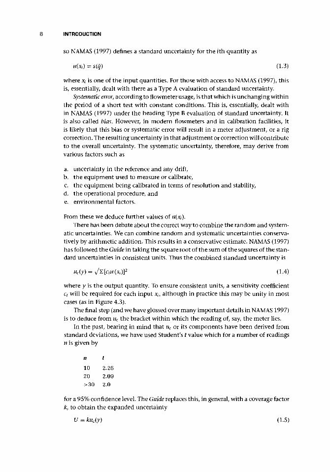
INTRODUCTION
so NAMAS (1997) defines a standard uncertainty for the /th quantity as
(1.3)
where xt is one of the input quantities. For those with access to NAMAS (1997), thisis, essentially, dealt with there as a Type A evaluation of standard uncertainty.
Systematic error, according to flowmeter usage, is that which is unchanging withinthe period of a short test with constant conditions. This is, essentially, dealt within NAMAS (1997) under the heading Type B evaluation of standard uncertainty. Itis also called bias. However, in modern flowmeters and in calibration facilities, itis likely that this bias or systematic error will result in a meter adjustment, or a rigcorrection. The resulting uncertainty in that adjustment or correction will contributeto the overall uncertainty. The systematic uncertainty, therefore, may derive fromvarious factors such as
a. uncertainty in the reference and any drift,b. the equipment used to measure or calibrate,c. the equipment being calibrated in terms of resolution and stability,d. the operational procedure, ande. environmental factors.
From these we deduce further values of u(xt).There has been debate about the correct way to combine the random and system-
atic uncertainties. We can combine random and systematic uncertainties conserva-tively by arithmetic addition. This results in a conservative estimate. NAMAS (1997)has followed the Guide in taking the square root of the sum of the squares of the stan-dard uncertainties in consistent units. Thus the combined standard uncertainty is
My) = y/VlcMxi)]* (1.4)
where y is the output quantity. To ensure consistent units, a sensitivity coefficientCi will be required for each input xif although in practice this may be unity in mostcases (as in Figure 4.3).
The final step (and we have glossed over many important details in NAMAS 1997)is to deduce from uc the bracket within which the reading of, say, the meter lies.
In the past, bearing in mind that uc or its components have been derived fromstandard deviations, we have used Student's t value which for a number of readingsn is given by
n
1020> 3 0
t
222
.26
.09
.0
for a 95% confidence level. The Guide replaces this, in general, with a coverage factork, to obtain the expanded uncertainty
U = kuc(y) (1.5)

1.6 WHAT IS A FLOWMETER?
The recommended value is k = 2, which gives a confidence level of 95.45% taken as95%, assuming a Normal distribution. If this assumption is not adequate, then weneed to revert to Student's t.
The net result is that the assumption of a factor of 2 has now been given asystematic basis. The reader who is interested in more details about the basis ofNormal and t distributions is referred to Appendix l.A.
1.5 SENSITIVITY COEFFICIENTS
Suppose that output quantity, a flow rate, has the relationship
y = xplxq
2xr3xs
4 (1.6)
then if x2, x3f and *4 are held constant, we can differentiate y with respect to X\ andobtain the partial derivative. This is the slope of the curve of y against X\ when theother variables are kept constant. It also allows us to find the effect of a small changein Xi on y. This slope (or partial derivative) is the sensitivity coefficient cx for xx andmay be found by calculation. It will have the value cx — px[p~r]x\x\x\t where thevalues of xx, Xz, X3, and X4 will be at the calibration point and may be dimensional.In some cases, it may be a known coefficient (e.g., a temperature coefficient of ex-pansion). For cases where it is difficult to calculate, it may be possible to find thecoefficient by changing xx by a small amount and observing the change in y. In somecases, the sensitivity coefficient may provide a conversion between different sets ofunits (e.g., where output quantity or velocity may be obtained from a dimension, apressure, a movement, or a voltage).
1.6 WHAT IS A FLOWMETER?
We take as a working definition of an ideal flowmeter:
A group of linked components that will deliver a signal uniquely related tothe flow rate or quantity of fluid flowing in a conduit, despite the influence ofinstallation and operating environment.
The object of installing a flowmeter is to obtain a measure of the flow rate, usuallyin the form of an electrical signal, which is unambiguous and with a specified ex-panded uncertainty. This signal should be negligibly affected by the inlet and outletpipework and the operating environment. Thus the uncertainty of measurementof a flowmeter should be reported as y ± U, where U, the uncertainty band, mighthave a value of, say, 0.5%, and it should be made clear whether this is related torate, full-scale deflection (FSD) or other value that might be a combination of these[e.g., in the form ±a (rate) ±b (FSD)]. The range should be given (e.g., Im3 /h to20m3/h).
The statement of performance should include the coverage factor k = 2 and thelevel of confidence of approximately 95%, and, if appropriate, the authority thataccredited the calibration facility (national or international).

10 INTRODUCTION
In addition, the ranges of properties for which it can be used should be speci-fied, such as fluid, flow range (beyond calibration), maximum working pressure,temperature range of fluid, and ambient temperature range.
It is useful to introduce two factors that define the response of flowmeters, al-though they are most commonly used for linear flowmeters with pulse output. TheK factor is the number of pulses per unit quantity. In this book, we shall take it asnumber of pulses per unit volume when dealing with turbine and vortex meters:
PulsesTrue volume
whereas the meter factor is usually defined as
True volumeMeter factor = Indicated volume
The reader should keep a wary eye for other definitions of meter factor such as thereciprocal of the K factor.
Let us take a specific example of a fictitious, but reasonably realistic flowmeter.In Figure 1.2(a), a typical flowmeter envelope is shown. It defines an approximatelylinear flowmeter with a 10:1 turndown and an uncertainty of ±1% of rate with aconfidence level of 95% against a traceable standard calibration. This is a reasonableperformance for a flowmeter and probably satisfies most requirements in industry.This, let us assume, is the performance specification the manufacturer carries in itssales literature. Actually the characteristic of the flowmeter may be the curve shownin Figure 1.2(a). If the company works to a high standard of manufacture, then thecompany may know that this characteristic lies within close tolerances in all cases.It may, therefore, only be necessary for the manufacturer to calibrate each flowmeterat, say, 90% of FSD, or 50% and 90% of FSD, in order to make the claim that thecharacteristic falls within the envelope specified in the sales literature.
If the meters are actually of this standard, it may well be feasible to calibratethem in much greater detail so that a 5-, 10-, or even 20-point calibration mayprovide a characteristic that ensures that the reading is known to, say, ±0.2%. Thevalues obtained from the calibration will then be programmed into a flow computer,which will interpret each reading of the flowmeter against this look-up table. Sincewe are comparing the flowmeter's signal to a linear one, if it were without error itwould also be linear. Consequently, companies sometimes record linearity withintheir literature. In this case, it would also be ±1% with a 10:1 turndown.
The envelope that has been discussed gives the uncertainty at each flow ratein terms of the actual flow rate. Because of the physical basis of some flowmeters,this method is not appropriate, and the uncertainty may then be given in terms ofthe full scale. Figure 1.2(b) shows such an envelope where the performance of theflowmeter would be defined as ±1% FSD. It is apparent that the uncertainty in theflowmeter's reading at, say, half scale is ±2% of rate and at 20% of reading will beas much as ±5% of rate. The problem often arises wherein the user has a particularflow range that does not match that of the actual instrument. The user's full flowmay only be at 60% of the instrument's range, and so for the user the instrumenthas an uncertainty, at best, of 1.7% of rate.

1.6 WHAT IS A FLOWMETER? 11
Uncertainty inreading
(a)
- 2 %
FLOWMETER PRECISIONENVELOPE
- _ iqo%
50% FULL SCALE
FLOWMETER CHARACTERISTICRELATIVE TO IDEAL
Uncertainty inreading
-5% -
, FLOWMETER PRECISIONENVELOPE
Uncertainty inreading
(c)
- 2 %
FLOWMETER PRECISIONENVELOPE
^MINIMUM ^TRANSITION ^NORMAL
2% 20% 50% 100%
FULL SCALE
Figure 1.2. Required envelope for a flowmeter. (a) Envelope as a percentage ofrate, (b) Envelope as a percentage of FSD. (c) Stepped envelope with increaseduncertainty at low range values.
A third type of envelope is shown in Figure 1.2(c). This is particularly commonin the specifications for water and gas meters. In the example shown, the meter hasan uncertainty of ±2% of rate from full flow down to 20%. Below this value of flowrate, the uncertainty is ±5% of flow rate down to 2% of range. In practice, a metermight have more steps in its envelope.
In many cases, the specification of uncertainty by the manufacturer may be acombination of these. As indicated earlier, it is common to have an uncertaintythat combines a value based on rate and another on full-scale deflection. In add-ition, there may be allowances to be added for zero drift, temperature change,and, possibly, even pressure change. In some flowmeters, viscosity is important butis probably accommodated by charts showing the variation in performance withviscosity.
One note of caution! Clever electronics can take any signal, however non-linear, and straighten the characteristic before the signal is output. Suppose sucha procedure were used for the characteristic in Figure 1.2(a), below 10% of range.

12 INTRODUCTION
The characteristic is probably very sensitive to minor variations in this region,and any attempt to use the characteristic could lead to disguised, but serious,errors.
Variation of temperature and pressure can have effects on the performance of aflowmeter, as can humidity, vibration, and other environmental parameters (Baker1988/9).
Often the units used in a manufacturer's catalog are not those that you havecalculated. For this reason, conversion factors that provide conversions to four sig-nificant figures of flow rate, velocity, temperature, pressure, length, etc., have beenincluded in Table 1.1. If not otherwise specified the International System of units(SI) based on meter, kilogram, second is assumed.
Table 1.1. Conversion for some essential measurements from Imperial, U.S.,and other units to metric, to four significant figuresLength 1 ina = 25.4 mm
1 ft = 0.3048 mVolume 1 ft3 = 0.0283 m3
1 ft3 = 28.321 (liter)lbbl (barrel) = 0.1590 m3
Mass l lb = 0.4536 kg1 long ton (2,240 lb) = 1,016 kg1 short ton (2,000 lb) = 907.2 kg1 metric tonne (2,205 lb) = 1,000 kg
Density 1 lb/ft3 = 16.02 kg/m3
Temperature (Temperature in°F — 32)/1.8 = Temperature in °CPressure 1 psi = 6,895 N/m2
Viscosity Dynamic viscosity: SI (metric) unit is the Pascal second(Pas) to which the more common unit, the centipoise (cP),is related by 1 cP = 10~3 Pas.
Kinematic viscosity: SI (metric) unit is m2/s to which themore common unit, the centistoke (cSt), is related by1 cSt = 10~6 m2/s = 1 mm2/s.
lft/s = 0.3048 m/s1 ft3/s (1 cusec) = 0.02832 m3/s1 Imp gal/s = 0.004546 m3/s1 Imp gal/s = 4.546 1/s1 U.S. gal/s = 0.003785 m3/s1 U.S. gal/s = 3.785 1/s1 Imp gal/h = 0.004546 m3/h1 Imp gal/h = 4.546 1/h1 U.S. gal/h = 0.003785 m3/h1 U.S. gal/h = 3.785 1/h
Mass flow rate 1 lb/h = 0.4536 kg/h1 lb/s = 0.4536 kg/s
a An approximate conversion is 4 in. to 100 mm.
VelocityVolumetric flow rate

1.7 CHAPTER CONCLUSIONS 13
1.7 CHAPTER CONCLUSIONS (FOR THOSE WHO PLAN TO SKIPTHE MATHEMATICS!)
I have tried to bring together, within the scope of this book, essential informationfor all who may have dealings with flowmeters and flow measurement (although Ihave tried to avoid duplicating too much of the excellent and practical informationgiven by Miller 1996). For this reason, the chapters not only address the technicalaspects but also the selection, maintenance, calibration, and typical applications ofthe various meters. There is also a section on manufacture and production. I hopethat the book will provoke the prospective entrepreneur, the small and medium-sizedenterprises (SME), or the major instrument company to assess the market needs andthe relevant development and production needs of their companies for new devices.
One plea regarding manufacturers' brochures is in order. It would be helpful tohave a standard format for the core information to which the manufacturer couldadd special features and presentation to reflect customer demands (e.g., from differ-ent countries and industries). I often find myself faced with two catalogs from thesame manufacturer. I search them to find how they differ. They clearly are printeddifferently, and yet it is not clear whether they refer to different meters. Do just thecatalogs differ, or is there a difference between the flowmeters described in each cat-alog? This may seem an unlikely problem, but the preparation of this book confirmsthat confusing catalogs are still with us.
The corollary of the last plea (for a readable and complete brochure) is that themanufacturer needs to be told everything about the fluid and the installation inorder to decide whether the meter can handle the requirements. We shall return tothis point in much greater detail in Chapter 3.
I have endeavored to reflect the requirements of standard documents, but thereader is encouraged to obtain relevant standards. A partial list is included togetherwith a bibliography at the end of this book. Standards organizations and professionalbodies have produced a range of essential documents that cover many aspects of flowmetering. Upp (1993) provides a useful digest of some of the documents such as API'sManual of Petroleum Measurement Standards, AGA documents which for many flowmeasurement applications (e.g., Section 14.3) are the same as API, and ASME andISA. Another example from the United Kingdom is IGE (1988), which recommendsstandards of good practice and provides an extremely thorough statement on gasmeter installation, which, although not carrying the wider backing of a standard,is clearly very authoritative and should provide a companion volume. Such topicsas commissioning and maintenance are covered, and the manual encourages pro-cedures for routine maintenance and record keeping as do I (cf. Olsen 1974, Kulin1975).
As the reader moves into the following chapters, two sets of information may beuseful. Table 1.1 lists the conversion factors for Imperial, U.S., and metric units, andTable 1.2 relates volumetric and mass flow rate to linear velocity in various sizes oftube (Baker 1988/9). It is common in flow measurement to require the velocity offlow, and Table 1.2 provides an order of magnitude.
Finally, the whole matter of accuracy and the limits of accuracy, when relatedto all the parameters that influence a flowmeter's operation, remains an area withunanswered questions.

Table 1.2. Velocity in pipes for various flow rates to two significant figures
Mean Velocity (m/s) in a Circular Pipe of Diameterm3/h°
Very 10~3
lowlO-2
0.11
10100
10001 0 4
1 0 5
Veryhigh 106
1/min
0.017
0.171.7
17170
17001.7 x 104
1.7 x 10⁵
1.7 x 10⁶
1.7 x 10⁷
gal/min gal/min
3.7 x lO"3 4.4 x 10~3
3.7 x 10~2 4.4 x 10"2
0.37 0.443.7 4.4
37 44370 440
3700 44003.7 x 104 4.4 x 10⁴
3.7 x 10⁵ 4.4 x 10⁵
3.7 x 10⁶ 4.4 x 10⁶
Reproduced from Baker (1988/9) with permission
ft3/min
5.9 x lO-4
5.9 x 10"3
5.9 x 10"2
0.595.9
59590
59005.9 x 104
5.9 x 10⁵
10 mm
3.5 x 10"3
3.5 x 10~2
0.353.5
35350
35003.5 x 104
3.5 x 10⁵
3.5 x 10⁶
25 mm
5.7 x lO-4
5.7 x lO"3
5.7 x 10"20.575.7
57570
50 mm
1.4 x lO-4
1.4 x 10"3
1.4 x 10"2
0.141.4
141 4 0
of Professional Engineering Publishing.a Since water has a density of 1,000 kg/m3 (approximately), the mass flow rate in kilograms per
100 mm 200 mm
3.5 x 10
3.5 x 103.5 x 103.5 x 10
0.353.5
353 5 0
hour of
- 5
-4 8.8 x lO-5
- 3 8.8 x lO-4
-2 8.8 x lO-3
8.8 x 10"2
0.888.8
88880
500 mm
1.4 x lO-5
1.4 x 10"41.4 x 10~3
1.4 x 10"2
0.141.4
141 4 0
water may be obtained by
1000 mm
3.5 x lO-5
3.5 x lO-4
3.5 x lO-3
3.5 x 10"2
0.353.5
35
350
multiplying
2000 mm
8.8 x lO-5
8.8 x lO-4
8.8 x lO-3
8.8 x lO-2
0.888.8
88
this column

1.A.1 INTRODUCTION 15
1.8 MATHEMATICAL POSTSCRIPT
I have left this note to the end so that those who are not concerned with advancedmathematical concepts can ignore it.
I have included essential mathematics in the main text of the book. In certainflowmeters, the mathematical theory is more complex (e.g., the turbine meter),and the theory has, accordingly, been consigned to an appendix after the relevantchapter.
One important and interesting mathematical approach, which starts to developa unified theory of flow measurement, was first suggested by Shercliff (1962) andsignificantly extended by Bevir (1970). Both applied it to electromagnetic flow-meters where it has been highly successful. Hemp (1975) has also applied this theoryto electromagnetic flowmeters, but he has developed the theory for other types offlowmeter: ultrasonic (1982), thermal mass (1994a), and Coriolis (1994b, and Hempand Hendry 1995). In Chapter 12, on electromagnetic flowmeters, an appendix de-scribes the essential mathematics. The weight function developed in this theoryprovides a measure of the importance of flow in each part of the meter with respectto the overall meter signal. The flow at each point of a cross-section is weighted withthis function. Ideally the weighting should result in a true summation of the flowin the meter to obtain a volume flow rate. It has been possible to approach this idealfor the electromagnetic flowmeter.
For the other types of meters, the reader will be given only a brief explanationand will be referred to relevant papers. This is partly for want of space in this bookand partly because the theory, although interesting, is still being developed and maynot yet have reached a sufficiently significant stage for the designer.
A second mathematical physics theory, first (to my knowledge) applied by Hemp(1988) to flow measurement, is reciprocity. This, essentially, states that if you applya voltage to one end of an electrical network and measure the current at the otherend, you find that by reversing the ends and hence the direction you obtain thesame relationship. Hemp has proposed this as a means of eliminating some errorsin flowmeters to which the theory is applicable.
APPENDIX 1.A
Statistics of Flow Measurement
1.A.1 INTRODUCTION
The main needs of the engineer are to
• understand and be able to give a value to the uncertainty of a particular measure-ment;
• know how to design a test to provide data of a known uncertainty;• be able to combine measurements, each with its own uncertainty, into an overall
value; and

16 INTRODUCTION
• determine the absolute accuracy of an instrument at the end of a traceable ladderof measurement.
The international and national documents set the recommended approach forflow metering. Most standard statistics books will provide the essentials (Rice 1988;cf. Campion et al. 1973, which is often quoted but may not be easy to obtain), butgood school texts may be more accessible (Crawshaw and Chambers 1984, Eccleset al. 1993a, 1993b). Hayward (1977) is an extremely well written and elegant littlebook, which deserves to be updated and reprinted; Kinghorn (1982) provides a well-written and useful brief review of the main points; and Mattingly (1982) addressessome of the problems concerned with transfer standards.
1.A.2 THE NORMAL DISTRIBUTION
The Normal distribution, Figure l.A.l(a), is also known as the Gaussian distributionafter Carl Friedrich Gauss, who proposed it as a model for measurement errors (Rice1988). The notation used for the Normal curve is N(/x, a2) which is the distribution
under the curve
<t>(0.5) = 0.6915PROBABILITY OF READING
LYING IN UNSHADEDAREA = 0.3085
SHADED AREA- 0.950
ARE A =0.025 AREA - 0.025
Figure l.A.l. The Normal distribution.
f(*) = (l.A.l)
where \x is the mean value of the data, anda2 is the variance. Alternatively, a is thestandard deviation for the whole popula-tion. We can simplify the curve (normalizeit) by putting z = (x — fi)/a and obtaining[Figure l.A.l(b)]
0(z) = 1 (1.A.2)
With the form of Equation (1.A.2), thecurve does not vary with the size of the pa-rameters fi and o.
What the curve tells us (in relation to in-strument measurements) is that the statisti-cal chance of an instrument reading givinga value near to the mean /x is high, but thefarther away the reading is from the mean,the less the chance is of its occurring (indi-cated by the curve decreasing in height thefurther one moves from the mean), and asvalues of the reading get farther still fromli, so the chance gets less and less.
The area under the curve of Equation(1.A.2) [Figure l.A.l(b)], which reaches toinfinity each way, is unity, and this is the
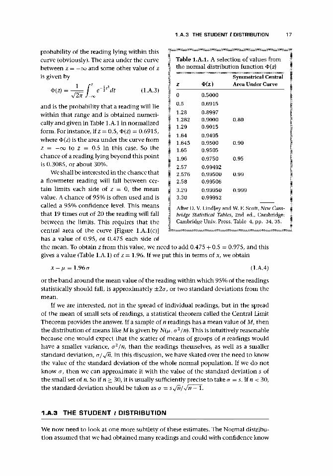
1 .A.3 THE STUDENT t DISTRIBUTION 17
probability of the reading lying within thiscurve (obviously). The area under the curvebetween z = —oo and some other value of zis given by
= — fy/2jT J-o
Table l.A.l. A selection of values fromthe normal distribution function <f>(z)
Symmetrical Centralz 3Hz) Area Under Curve
dt (1.A.3)
and is the probability that a reading will liewithin that range and is obtained numeri-cally and given in Table l.A.l in normalizedform. For instance, if z = 0.5, <I>(z) = 0.6915,where <I>(z) is the area under the curve fromz = -oo to z = 0.5 in this case. So thechance of a reading lying beyond this pointis 0.3085, or about 30%.
We shall be interested in the chance thata flowmeter reading will fall between cer-tain limits each side of z = 0, the meanvalue. A chance of 95% is often used and iscalled a 95% confidence level. This meansthat 19 times out of 20 the reading will fallbetween the limits. This requires that thecentral area of the curve [Figure l.A.l(c)]has a value of 0.95, or 0.475 each side ofthe mean. To obtain z from this value, we need to add 0.475 + 0.5 = 0.975, and thisgives a value (Table l.A.l) of z = 1.96. If we put this in terms of x, we obtain
0
0.5
1.281.2821.29
1.641.6451.65
1.96
2.572.5762.58
3.293.30
0.5000
0.6915
0.89970.90000.9015
0.94950.95000.9505
0.9750
0.994920.995000.99506
0.999500.99952
0.80
0.90
0.95
0.99
0.999
After D. V. Lindley and W. F. Scott, New Cam-bridge Statistical Tables, 2nd ed., Cambridge:Cambridge Univ. Press. Table 4, pp. 34, 35.
x-ti = 1.96a (1.A.4)
or the band around the mean value of the reading within which 95% of the readingsstatistically should fall, is approximately ±2a, or two standard deviations from themean.
If we are interested, not in the spread of individual readings, but in the spreadof the mean of small sets of readings, a statistical theorem called the Central LimitTheorem provides the answer. If a sample of n readings has a mean value of M, thenthe distribution of means like M is given by N(^, a2/n). This is intuitively reasonablebecause one would expect that the scatter of means of groups of n readings wouldhave a smaller variance, o1In, than the readings themselves, as well as a smallerstandard deviation, cr/y/n. In this discussion, we have skated over the need to knowthe value of the standard deviation of the whole normal population. If we do notknow o, then we can approximate it with the value of the standard deviation s ofthe small set of n. So if n > 30, it is usually sufficiently precise to take a — s. If n < 30,the standard deviation should be taken as a = s^Jnj^Jn — 1.
1.A.3 THE STUDENT t DISTRIBUTION
We now need to look at one more subtlety of these estimates. The Normal distribu-tion assumed that we had obtained many readings and could with confidence know

18 INTRODUCTION
-4 -3 -2 -1
1.96 2.23
Figure l.A.2. Student's t distribution curves com-pared with the Normal curve. Note p = 5% as relatedto Table l.A.2 for both tails.
that they formed a Normal distribution. Wecan agree that if the error is random, thenit is a fair assumption that many readingswould form a Normal distribution. How-ever, often we have only a few readings,and these may not be uniformly distributedwithin the curve of Figure l.A.l. Too manymay lie outside the 1.96 a limit. For thisreason, we use the Student t distribution,which allows for small samples on the as-sumption that the distribution, as a whole,is Normal. Figure l.A.2 shows the effect ofthe small number of readings. Since, witha small number of readings, one has to besubtracted from all the others to obtain a
mean, the number of independent values is one less than the number of readings,and so the statisticians say that there is one less degree of freedom than the numberof readings. In Figure l.A.2, v is the symbol for the degree of freedom, and v = n - 1,where n is the number of readings. For v -* oo, the t distribution tends to a Normalcurve with mean zero and variance unity.
Figure l.A.2 shows clearly the larger area spreading beyond the Normal curve inwhich the readings may lie and the reason for the greater uncertainty. The curves areused in a similar way to the Normal curve, but, as an alternative, Table l.A.2 providesthe information we need. If we have 10 readings, say, and so select the value of v = 9for the degree of freedom, and if we wish to find the limits for a confidence levelof 95%, we shall need to use the 5% column. We obtain t = 2.262, which we canapply to obtain the limits for a 95% confidence of ±2.262 a/y/n on the mean valuesof groups of readings, where n is the number of readings in the group. We should
Table l.A.2. A selection of values from the student t functionp(%) (Total)
n
23510
203061121
oo
V
1249
192960120
oo
20
10
3.0781.8861.5331.383
1.3281.3111.2961.289
1.282
10p/2
5
6.3142.9202.1321.833
1.7291.6991.6711.658
1.645
5(%) (per tail)
2.5
12.71
4.303
2.776
2.262
2.093
2.045
2.000
1.980
1.960
1
0.5
63.66
9.925
4.604
3.250
2.861
2.756
2.660
2.617
2.576
0.1
0.05
636.6
31.60
8.610
4.781
3.883
3.659
3.460
3.373
3.291
After D. V. Lindley and W. F. Scott, New Cambridge Statistical Tables, 2nded., Cambridge: Cambridge Univ. Press, Table 10, p. 45.

1.A.4 PRACTICAL APPLICATION OF CONFIDENCE LEVEL 19
note, however, that the 95% confidence level from Table 1.A.2 gives a t value thatvaries little from 2.0 if v > 20. The limits for 95% confidence will then be ±2.0 o/ Jnon the mean values of groups of readings.
I have always been puzzled by the name Student, but Eccles et al. (1993b) explainthat the originator of this technique was William S. Gosset, born 1876, who usedthe pseudonym Student.
1.A.4 PRACTICAL APPLICATION OF CONFIDENCE LEVEL
The method described in Section 1.4 leads to the following steps (cf. Hayward 1977):
i. Write down systematic uncertainties and derive the standard uncertainty foreach component,
ii. Write down random uncertainties and derive the standard uncertainty for eachcomponent,
iii. Calculate the combined standard uncertainty for uncorrelated input quantities(and refer to NAM AS 1997 if correlated),
iv. Obtain the expanded uncertainty using k = 2 for 95% confidence.
Taking a simple example, where we need to revert to t, suppose that we obtaina series of volumetric flow readings from a 50 mm ID flowmeter with the flow set at10m3/h:
10.06, 10.01, 9.95, 9.99, 9.85, 10.02,10.03,10.12, 9.90, 9.98.
The results are plotted in Figure l.A.3. The mean of these readings is 9.991, andthe standard deviation is 0.07752. We could thus conclude that the true reading ofthis meter fell in the bracket 9.991 ± 2.262 x 0.07752/V9 = 9.991 ± 0.05845, orbetween 9.93 and 10.05 with a 95% confidence. This fairly brackets the value of10 m3/h.
The actual readings should have all fallen within 9.991 ± 0.07752, or 9.91 and10.07. In fact three fell outside this bracket - rather higher than the 1 in 19 impliedby the 95% confidence level. We might wish to look more closely at the procedure
m3/h
10.15 - -
10.10 - -
10.05 + X
10.00
9.95 - - X
9.90 - :
9.85 + X
' 1 1 1 1 1 1 1 1 1 |—TIMESUCCESSIVE CALIBRATION RUNS
Figure l.A.3. A set of flowmeter test readings (after Kinghorn 1982) for a fixed flow rate.

20 INTRODUCTION
for obtaining these results since this suggests a possible problem with the means forobtaining the data.
1.A.5 TYPES OF ERROR
There are essentially four types of error (Kinghorn 1982).
• Spurious errors result from obvious failures, obvious in the sense that they can beidentified and documented. Readings with these should be eliminated.
• Random errors cause a variation in the output reading even when the inputparameter has not changed.
• Constant systematic error, which is also called bias, may vary over the range but isconstant in time, and could, in principle, be corrected out of the reading.
• Variable systematic error (bias) slowly varies with time, usually in a consistentdirection, and may be caused by wear in bearings of a rotating meter, fatigue incomponents of a vibrating meter, erosion of geometry, etc.
Figure 1.A.4 illustrates these errors. Clearly one of the readings is so far out thatthere must be some explanation other than randomness. It is comforting to knowthat some of the most eminent experimentalists of the past have had cause to discardreadings in critical experiments!
The scatter around the mean line will provide the basis of the calculation whichwe did in Section l.A.4. The constant systematic error (bias) can be seen and could bebuilt into a flow computer. The change in the mean value with time shows the chang-ing systematic error, which is, in part, the reason for regular recalibration of meters.
The repeatability is related to the closeness of readings. If we expect a reading tolie within a band given by ±2s, the worst case difference between successive readingsthat fall within this band would be 45 [(2 x 2)5], but a less extreme working value isobtained from the root of the sum of the squares (or the quadrature; cf. Pythagorasand the length of the hypotenuse):
J{2s)2 + (25)2 or 2V25
TBIAS
RANDOMERROR
4OUTLIER
SPURIOUSERROR
TRUE VALUE
X
RANDOMUNCERTAINTY
MEAN- MEASURED
VALUE
NOTE DRIFT OFMEAN CAUSING
A CHANGE INBIAS
TIME
Figure l.A.4. Diagram to show the various types of error (after Kinghorn 1982).

1.A.7 UNCERTAINTY RANGE BARS, TRANSFER STANDARDS, AND YOUDEN ANALYSIS 21
1.A.6 COMBINATION OF UNCERTAINTIES
If we combine uncertainties due to the nature of a flowmeter;s operating equation,then we take the following approach. Suppose that the flowmeter has the equation
n v vnv vm /-i A r \Lit) — ^ \ ^0 ^3 A I 1«A« J I
To obtain the uncertainty in qv, we need the partial derivative of qv with respect to X\,x2, etc. The required result can be achieved, either by differentiating the equationas it stands or by first taking logarithms of both sides. We shall skip this and gostraight to the result:
uc(qv) nu(x2) ± u(x3) ± mu(x4) (1.A.6)
The problem with this equation is that the arithmetic sum of the uncertainties isusually overpessimistic. It is, therefore, recommended that they be combined inquadrature, or by the root-sum-square (rss) method. This leads to the followingequation:
\ |(nu{x2)\{ x2 ) \ x3
There are complications beyond thisequation. x2 may appear in the equation asXs + *6- In this case, x$ + Xe will need to bedealt with first and will require careful con-sideration as to whether the actual errors inthese quantities are combining, canceling,or random.
|V^VFLOW RATE
(a)
(1.A.7)
TRUE' VALUE
TIME
1.A.7 UNCERTAINTY RANGEBARS, TRANSFER STANDARDS,AND YOUDEN ANALYSIS
It is sometimes useful to indicate the rangeof uncertainty that has been estimatedfrom the experimental method in eachreading. This can be done by using barsthat give uncertainty limits on each experi-mental point. This will then indicate, for aparticular flow rate, the likely uncertaintyin the reading. This is shown in Figurel.A.5(a). In some cases where flow ratevaries, there may be an uncertainty in bothprimary flow rate measurement and read-ing of second meters. In this case, therewill need to be uncertainty bars in both
SECONDARYMETER
READING
(b) PRIMARYMETER
READING
Figure l.A.5. (a) Uncertainty limit bars on readings.(b) Uncertainty limit bars on both flow rate and read-ings.

22 INTRODUCTION
71.7r
71.6
= 71.5445
71.5
71.4MAY MAY JUN SEP NOV DEC JAN FEB FEB
| 3 | 20 | 7 | 28 | 17 | 21 | 6 | 8 I 4 |
DATE
(a)
1.005r
1.004
85 1.00372
1.003
(b)
(C)
1.002
Tr 2cr
MAY MAY JUN SEP NOV DEC JAN FEB FEB1-3 1 20 1 7 1 28 | 17 I 21 | 6 I 2 I 4 I
DATE
METER FACTOR MTRN©1
Figure l.A.6. Turbine meter as a transfer standard (from Mattingly 1982; repro-duced with the author's permission), (a) Typical turbine meter control chartfor meter factor, (b) Typical turbine meter control chart for ratio, (c) Graphicalrepresentation of the Youden plot.

1.A.7 UNCERTAINTY RANGE BARS, TRANSFER STANDARDS, AND YOUDEN ANALYSIS 23
directions, and the rectangle [Figure l.A.5(b)] will define the limits of the possibleuncertainty. In other words, the maximum uncertainty will have been obtained byquadrature.
Mattingly (1982) describes the procedure for checking the validity of differentflow measurement laboratories using a Measurement Assurance Program (MAP) [orProficiency Testing as referred to by Mattingly in a recent draft report on the ap-proach of the National Institute of Standards and Technology (NIST)] where a good-quality flowmeter acting as a transfer standard is exchanged between laboratories.Figure l.A.6(a) shows the results of such a cycle of checks, and the bars on theexperimental points presumably indicate the uncertainty of the turbine meter at aparticular laboratory. Various people have suggested the use of two flowmeters usu-ally in series, but as a possible alternative in parallel, to enhance the accuracy of atransfer standard. In this case, the ratio of the signals from the two meters will givean indication as to whether there has been a shift in either, and, if there has notbeen, the reading of the meters will provide, with greater confidence, the accuracyof the facility. In Figure l.A.6(b), Mattingly (1982) gave a typical control chart forthe ratio of a pair of National Bureau of Standards turbine meters. If the ratio fallsoutside an agreed tolerance band, the cause of the error will need to be found beforeconfidence in the meter readings is restored.
For laboratory comparison, the transfer package with two meters should be runat one or two agreed flow rates. The position of the two flowmeters may be inter-changed to obtain a second set of data. Using the Youden analysis in Figure l.A.6(c),each laboratory is represented by a single point (1, 2, 3, etc.) resulting from plot-ting the meter factor of the two meters on the two axes. It is apparent that theposition of the points relates to the type of error. Essentially, if the points lie inquadrants I or III, then the meters are reading the same, and the error can be at-tributed to the flow rig. If the readings are in quadrants II or IV, the flowmeters arenot agreeing, and the error may be due to a malfunction in one of them. The reader isreferred to Mattingly's (1982) article for further details of this procedure (cf. Youden1959).

CHAPTER S
Fluid Mechanics Essentials
2.1 INTRODUCTION
In a recent book (Baker 1996), I provided an introduction to fluid mechanics andthermodynamics, particularly aimed at instrumentation. I do not, therefore, proposeto repeat what is written there but rather to confine myself to essentials. In addition,Noltingk (1988) has provided a very valuable handbook on general instrumentation.In this book, I shall use the term fluid to mean liquid or gas and will refer to eitherliquid or gas only when the more general term does not apply.
2.2 ESSENTIAL PROPERTY VALUES
Flowmeters generally operate in a range of fluid temperature from — 200°C (-330°F)to 500°C (930°F), with line pressures up to flange rating for certain designs. Typicalvalues of density and viscosity are given in Table 2.1.
It should also be noted that liquid viscosity decreases with temperature, whereasgas viscosity increases with temperature at moderate pressures. In common fluids,such as air and water, the value of viscosity is not dependent on the shear taking placein the flow. These fluids are referred to as Newtonian in their behavior as comparedwith others where the viscosity is a function of the shear taking place. The behaviorof such fluids, known as non-Newtonian, is very different from normal fluids likewater and air. Newtonian fluid behavior is a good representation for the behavior ofthe bulk of fluids.
2.3 FLOW IN A CIRCULAR CROSS-SECTION PIPE
An essential dimensionless parameter that defines the flow pattern at a particularvalue of the parameter is the Reynolds number
[I
where p is the density of the fluid, \± is the dynamic viscosity, and, when appliedto flow measurement, V is the velocity in the pipe, and D is the pipe diameter.Typical values of Reynolds number are: for water with /x/p = 10~6 m2/s, V =1 m/s(3.3 ft/s), D = 0.1 m (4 in.) Re= 105; and for air at ambient conditions with /x/p =1.43 x 10⁻⁵m2/s, V = 10 m/s (33 ft/s), D = 0.1 m (4 in.) Re = 0.7 x 10⁵.
24

2.3 FLOW IN A CIRCULAR CROSS-SECTION PIPE 25
Table 2.1. Typical values of viscosity (approximate values at 1bar)
Viscosity
WaterBenzeneOxygenNitrogenco2Air
Temperature(°C)
2020
0000
Density,9 (kg/m3)
1,000700
1.431.251.981.29
Dynamic,McP)1.0020.6470.0190.0170.0140.017
Kinematic,v (cSt)
1.0020.92
13.313.6
7.113.2
Adapted from Kaye and Laby (1966).
If Re is less than about 2,000, and the fluid has had a sufficient length of pipe toreach a steady state, it all moves parallel to the axis of the pipe. At the pipe wall, thefluid "sticks" to the pipe in, what is known as, a nonslip condition. The velocity ofthe fluid increases, therefore, from zero at the pipe wall to a maximum at the center,and the shape of the profile is parabolic. In this case, the flow is called laminar.
At about Re = 2,000, a major change takes place, and the smooth parallel natureof the flow gives way to eddies in the flow. These eddies mix the high velocity at thepipe axis with the lower velocity near the pipe wall. The resulting profile is flatter(although it still goes to zero at the pipe wall). When fully developed, this is knownas a turbulent profile. It is of a well-defined shape and with a known range of eddysizes. It may, therefore, be misleading to use the term turbulent profile for any otherprofiles created by upstream disturbances due to bends, etc. Between the turbulentflow and the laminar flow, there is a transition when the flow alternates randomly,in space and time, between laminar flow and turbulent flow.
Any flowmeter application to non-Newtonian fluids will need advice from theflowmeter manufacturer. It is probable that clear bore flowmeters, if applicable, willbe most suitable. A flowmeter with relatively low sensitivity to profile, such as elec-tromagnetic or multibeam ultrasonic designs, will be worth consideration providedthe fluid is conducting for the first type or transmits an adequate level of soundfor the second.
It is apparent from the calculations of Reynolds number for water and air that,in the majority of industrial applications, the flows will be turbulent, and, therefore,the behavior of the turbulent profile, and of flowmeters subject to it, is of primaryimportance to us.
For laminar flow, we can use the equation
V=V0 1 - [L. (2.2)
where Vo is the velocity on the axis of the pipe, r is the radial point at which we aremeasuring velocity, and R is the pipe radius and where V is zero at the wall of thepipe because of the nonslip condition for a fluid at a solid boundary.

26 FLUID MECHANICS ESSENTIALS
Table 2.2. Approximate turbulent velocity profiles from equation (2.4)
Re
nV/V[air =V/V[a.tr =
0.75R)0.758/?)
4 x 10³
6.01.0030.998
2.3 x 10⁴
6.61.0040.999
1.1 x 10⁵
7.01.0041.000
1.1 x 10⁶
8.81.0051.002
2.0 x 10⁶ to3.2 x 106
101.0051.002
The mean velocity in the pipe is then given by
" 2For turbulent flow an approximate curve-fit is
V= V0(l-r/R)l/n
(2.3)
(2.4)
where Vo is, again, the center line velocity, and we can relate n to Re from experi-mental data (Table 2.2). Note that pipe roughness, if the pipe is not hydraulicallysmooth, will also affect the profile.
This expression, therefore, provides not only a convenient, although approxi-mate, representation of the boundary layer shape but also an index adjustment toallow for the change in Reynolds number. The resulting profile shapes for the laminarand the turbulent regimes, based on Equation (2.4), are shown in Figure 2.1.
One interesting feature of these turbulent profiles is that the ratio of the velocityat about the 3/4 radius point to the mean velocity is approximately unity. The meanvelocity is given by
V In2
Hence
V/V =2n2 -a-r/R)\/n
(2.5)
(2.6)
Table 2.2 provides the values of this ratio for various values of Re and two radialpositions. Thus if a single measurement of velocity in a pipe is to be used to obtainthe mean of the velocity in a turbulent flow, a point at 0.7S8R may be found best.This figure will clearly be of importance when we consider where to position theprobes described in Chapter 18.
LAMINARRe < 2000
TURBULENTRe = 2.3x10 Re =1.1x10
Figure 2.1. Laminar and turbulent pipe profiles.
Re = 3.2x10

2.4 FLOW STRAIGHTENERS AND CONDITIONERS 27
A final important point about the profiles in Figure 2.1 is that there is muchdifference between the flows, even though they are drawn as smooth curves. In thelaminar profile, the fluid shears smoothly over itself, but it all moves essentiallyparallel to the axis of the pipe. In the turbulent profiles, the curves represent amean profile and ignore the turbulent eddies, which can be as much as 10% of thevelocity of the mean flow and cause fluctuations in all directions. In the context offlow measurement, this is particularly significant in that the meter must measureaccurately against this background fluctuation.
So far we have assumed that the pipe flow profile is fully developed. To achievesuch a profile requires an upstream straight length of pipe greater than may beavailable in many industrial flowmeter installations. 60D is sometimes quoted as aminimum requirement.
We, therefore, have a problem when installing a flowmeter in that the calibrationconditions for a fully developed profile are unlikely to be achieved in the installationand that the meter accuracy will be degraded. We have four options.
i. Find an installation point where fully developed flow occurs,ii. Calibrate the flowmeter with the upstream pipework (downstream has little effect
beyond a maximum of about 8D).iii. Take extensive measurements of the effects of bends, valves, T-pieces, multiple
bends, expansions, and contractions on a particular flowmeter design and allowfor the change in precision,
iv. Attempt to reorder the flow to recreate a turbulent profile of the sort used forcalibration.
Outside a few laboratory situations, (i) is probably unlikely to be an option, but(ii) may not be realistic or financially viable unless in situ calibration is possible. Op-tion (iii) will be a recurring theme through the discussion of most types of flowme-ters. An alternative approach is to compute the profiles resulting from pipe fittings.One example of such an approach is that of Langsholt and Thomassen (1991) whoused a commercially available computer program to obtain the flow downstream ofvarious piping fittings. Some indication that computer prediction and experimentgave similar swirl decay downstream of a double bend in perpendicular planes wasgiven, and 41D reduced the angle to 3.3° for measured values and 2.4° for simulatedvalues. Mottram and Rawat (1986) suggested that the swirl from two 90° bends inperpendicular planes is reduced by 50% in smooth pipes after L/D = 45 and inrough pipes after an L/D value in the range 10 to 20 (cf. however Mattingly et al.1987 who noted swirl effects on a turbine meter after 90D).
Langsholt and Thomassen (1991) also provided some flow contours at points ina complex pipe configuration. In the context of this chapter, it is important to givesome attention to (iv).
2.4 FLOW STRAIGHTENERS AND CONDITIONERS
Flow straighteners and flow conditioners have been used, for many years, to attemptto reorder a profile that has been disturbed by upstream fittings. The flow straightenerwas designed to remove swirl from the flow. Swirl, the bodily rotation of the fluid in
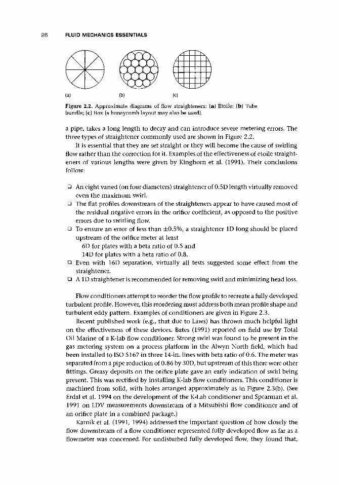
28 FLUID MECHANICS ESSENTIALS
(c)
Figure 2.2. Approximate diagrams of flow straighteners: (a) Etoile; (b) Tubebundle; (c) Box (a honeycomb layout may also be used).
a pipe, takes a long length to decay and can introduce severe metering errors. Thethree types of straightener commonly used are shown in Figure 2.2.
It is essential that they are set straight or they will become the cause of swirlingflow rather than the correction for it. Examples of the effectiveness of etoile straight-eners of various lengths were given by Kinghorn et al. (1991). Their conclusionsfollow:
• An eight vaned (on four diameters) straightener of 0.5D length virtually removedeven the maximum swirl.
• The flat profiles downstream of the straighteners appear to have caused most ofthe residual negative errors in the orifice coefficient, as opposed to the positiveerrors due to swirling flow.
• To ensure an error of less than ±0.5%, a straightener ID long should be placedupstream of the orifice meter at least
6D for plates with a beta ratio of 0.5 and14D for plates with a beta ratio of 0.8.
• Even with 16D separation, virtually all tests suggested some effect from thestraightener.
• AID straightener is recommended for removing swirl and minimizing head loss.
Flow conditioners attempt to reorder the flow profile to recreate a fully developedturbulent profile. However, this reordering must address both mean profile shape andturbulent eddy pattern. Examples of conditioners are given in Figure 2.3.
Recent published work (e.g., that due to Laws) has thrown much helpful lighton the effectiveness of these devices. Bates (1991) reported on field use by TotalOil Marine of a K-lab flow conditioner. Strong swirl was found to be present in thegas metering system on a process platform in the Alwyn North field, which hadbeen installed to ISO 5167 in three 14-in. lines with beta ratio of 0.6. The meter wasseparated from a pipe reduction of 0.86 by 30D, but upstream of this there were otherfittings. Greasy deposits on the orifice plate gave an early indication of swirl beingpresent. This was rectified by installing K-lab flow conditioners. This conditioner ismachined from solid, with holes arranged approximately as in Figure 2.3(b). (SeeErdal et al. 1994 on the development of the K-Lab conditioner and Spearman et al.1991 on LDV measurements downstream of a Mitsubishi flow conditioner and ofan orifice plate in a combined package.)
Karnik et al. (1991, 1994) addressed the important question of how closely theflow downstream of a flow conditioner represented fully developed flow as far as aflowmeter was concerned. For undisturbed fully developed flow, they found that,

2.4 FLOW STRAIGHTENERS AND CONDITIONERS 29
(a)
(b)
THICKNESS-0.13D
(c)
flow
VANES
\\ \
IZ77
ZZ77
for Re of about 0.9 x 10⁵, the profile was ap-proximated by n = 7A in Equation (2.4),compared with n = 7 in Table 2.2. Mea-surements of velocity and turbulence pro-files and of orifice plate performance weremade to determine the effect of an el-bow upstream of the tube bundle withvarious spacings between the elbow, theflow straightener, and the metering posi-tion. They confirmed the point that, eventhough the profile may be approximatelycorrect, the turbulence characteristics areunlikely to be correct, and the orifice plateappears to be influenced by both.
Laws and colleagues have done someuseful work on straighteners and condi-tioners (Laws 1991, Laws and Ouazzane1992, 1995b, 1995c). Her work initially,and rather unexpectedly, suggested thattube bundles of length recommended byISO 5167 (hexagonal pack of 19 tubes ofL > 20d), AGA(3), and ANSI/API 2530:1985(circumferential pack with L > lOd) arelittle more, and possibly less, effective thanone of only L = 1.25d. She found that thiswas as effective in swirl elimination and at-tenuation of profile nonuniformities. Shealso suggested that the AGA design wasmore effective and had a lower Ap. This ledher to suggest that perforated plates may bea better and more easily constructed option.
This observation was reinforced by workon the Zanker flow conditioner with thickerperforated plate, which performed, in somecases, better without downstream honey-comb (Laws and Ouazzane 1992). A crite-rion of ±6% of the fully developed pro-file 100D downstream was used to assesswhether the resultant Zanker profiles at8.5D were satisfactory. The reported experi-ments suggested that, for a 12-mm plate in a 100-mm line, the Zanker flow con-ditioner without downstream honeycomb performed better than with the honey-comb. Laws and Ouazzane (1995b) also suggested that a thick Zanker plate (10%of the pipe diameter) with upstream honeycomb flow straightener is preferable tothe Zanker straightener with thinner plate and downstream straightener. Not sur-prisingly, they suggested that the Laws plate is superior. In further tests, Laws andOuazzane (1995c) found that the etoile flow straightener was not a very good flow
= 0.13D
,PLATE
TABS
vortex tabs
Figure 2.3. Approximate diagrams of flow condition-ers: (a) Zanker; (b) K-Lab Mark 2; (c) Mitsubishi; (d)Laws (after Laws 1990, Laws and Ouazzane 1995a);(e) Vortab [reproduced with permission of Laaser(UK) Ltd.].

30 FLUID MECHANICS ESSENTIALS
conditioner, although it was effective as a straightener. They suggested that if theetoile is made with the vanes stopping short of the pipe axis, the wake from the hubof the etoile is removed and the performance is improved.
Laws (1990) described her new flow conditioner, which benefited from thesefindings. It has a central hole and two rings of holes on 0.4616D and 0.8436D. Theplate thickness is given as 0.123D and, for best performance, has an arrangement ofvanes and tabs as shown in Figure 2.3(d). The number of holes is 1:7:13 (or 1:6:12in later versions), the ratio of open area outer to inner ring is 1.385, and the ratio ofinner ring to central hole is 5.42. The total open area is 51.55%. Laws claims that theunit will be an enhancement to most flow installations, enabling flow conditionsto be maintained close to fully developed irrespective of the operating conditionsand thus minimizing errors due to installation effects. The loss coefficient is about1.4, and the claim appears to be made that with a flow distortion device 3D fromthe conditioner and the conditioner 3D upstream of the upstream pressure tappingof an orifice plate, the shift in performance is of order 0.2% (Laws and Ouazzane1995a).
Smith et al. (1989) proposed a different approach to the recreation of turbulentprofiles using vortex-generating devices. Their results looked promising for the con-ditioner 5D upstream of the flowmeter when they appear to claim less than 1% shift.The device consists of four axial swirl tabs of about ID length, which project about40% of the radius into the flow from the wall and are essentially a straighteningdevice to remove swirl. Two sets are recommended; they should be set at 45° relativeto each other. These are followed by, preferably, two sections of ID length each,with four trapezoidal tabs (vor-tabs) spaced around the circumference of the pipeand projecting inward with an angle of about 30° to the pipe wall in the generaldirection of the flow. Laws and Harris (1993) tested this device and considered thatit did quite well in recreating a turbulent profile but appeared uncertain of the sta-bility of the resulting profile. The loss is claimed to be only 0.7 dynamic heads. Acommercially available device, the Vortab [Figure 2.3(e)], appears to exploit the sameidea and consists of a ID straightening section followed by a 2D section with threesets of vor-tabs.
Gallagher et al. (1994) discussed the development of the Gallagher conditioner,which also consists of an antiswirl device, settling chamber, and profile device moun-ted sequentially in the pipe.
2.5 ESSENTIAL EQUATIONS
The continuity equation results from the classical physics concept that mass can nei-ther be created nor destroyed and so the same mass must pass through each pointin a pipe
Mass flow = qm = pqv = pVA (2.7)
and we can relate the velocity at different pipe sections 1 and 2 (Figure 2.4)
PlV1A1 = P2V2A2 (2.8)

2.5 ESSENTIAL EQUATIONS 31
•
Q{
r
i
\ v2
-
P2
—(f~1
DATUM
(a)
(b)
Figure 2.4. Duct sections, (a) Varying height and duct section, (b) Varying areaduct to show positions referred to in equations.
Bernoulli's equation can be derived from energy considerations (Baker 1996) andrelates the pressure change to the velocity change. Using Figure 2.4(a), we can relatepressure, velocity, and height above datum in a compressible fluid without flowlosses as
2d_p+ - v 2 ) = 0 (2.9)
This equation is known as the compressible fluid form of Bernoulli's equation. Ifp is constant for an incompressible fluid with constant density, then we can rewritethe Bernoulli equation as
(2.10)
Note from this, assuming that we can neglect changes in z, that, if the flow is broughtto rest, the resulting pressure, p0 is the total or stagnation pressure, the pressure whilefluid is flowing is the static pressure, and the difference, Ap = \pV2, is the dynamicpressure.

32 FLUID MECHANICS ESSENTIALS
If we neglect changes in height and combine Equations (2.8) and (2.10), weobtain an equation that gives the relationship between pressure change and flowrate through a duct such as in Figure 2.4(b)
( 2 - n )
Loss coefficients result, in real flows, from viscosity in the fluid, and it is essentialto know these losses in a piping system to ensure that the pump, or whatever createsthe flow, will be sufficient to maintain the required flow. To understand how tocalculate losses, the reader is referred to the excellent book by Miller (1990).
Thus all flowmeters create a flow loss, although clear bore meters do not signifi-cantly add to the loss due to an equal length of straight pipe. However, if the profileis highly disturbed and flow conditioning is used, these devices cause an additionalpressure loss which is given by
(2.12)
K may be up to order 5 for the devices in Figures 2.2 and 2.3, but for some flowconditioners it may be as much as 15 since the flow is effectively going through acontraction with very poor downstream pressure recovery.
For a fuller derivation of these equations, the reader is referred to Baker (1996)or other fluid mechanics books.
2.6 UNSTEADY FLOW AND PULSATION
In this section, we consider the effect of unsteadiness on flowmeters. The use of fluidinstability in flowmeters is covered in Chapter 11 where it is an essential part of themeter designs.
Most flowmeters are affected by unsteady or pulsatile flows for the followingreasons.
• Pulsatile flow affects the velocity profile in the pipe, and the distorted profile may,in turn, affect the flowmeter response. Hakansson and Delsing (1994) found thatflattening of the flow profile occurred due to the pulsating flows. This, in the caseof the ultrasonic flowmeter, causes incorrect averaging of the diametral beam.
• The characteristic of the meter may be nonlinear, and the resulting output aver-age will not correspond to that for the flow. The differential pressure flowmeterswith their square law are examples.
• The inertia of parts of the flowmeter or of the fluid may not allow the meterto track the pulsating flow correctly. The gas turbine meter is highly affected bythis. The importance of this effect in the orifice plate has been the cause of somediscussion in the literature for which the reader is referred to Mottram's papers.
• The natural operating frequency of the flowmeter may be near the pulsationfrequency, and this may cause aliasing or other errors. Vortex meters are sensitiveto such pulsations.

2.6 UNSTEADY FLOW AND PULSATION 33
TOTAL VOLUME VPRESSURE DROP Ap
CONSTRICTION
METERx
ADDEDCAPACITY
ABSOLUTELINE
PRESSUREP
SOURCEOF
PULSATION
Figure 2.5. Diagram to indicate symbols used in the Hodgson number calcula-tion.
• The secondary instrumentation may not be able to follow the pulsation, and, asa consequence, errors may be introduced. The manometer is the most obvioussecondary device to be affected, but pressure transducers, connecting leads, andother devices may also be affected.
One approach associated with Hodgson was developed to show how much damp-ing was needed to reduce pulsation to acceptable levels.
Mottram (1989) reviews some of the work on Hodgson's number (cf. Mottram1981) but makes the wise comment that "if you can't measure (the size of thepulsation) damp it" (Mottram 1992). The Hodgson number is given by (Figure 2.5)
VfApP
H= -L-t- (2.13)
where V is the total volume of pipework and other vessels between the source ofthe pulsation and the flowmeter position, Ap is the pressure drop over the samedistance, f is the frequency of the pulsation, qv is the volumetric flow rate, and pis the absolute line pressure. With this number, it is possible to plot curves to showthe likely error levels for various values of H (cf. Section 5.5 for orifice plates).
Mottram gives a simplified value for the damping based on the Hodgson number,allowing for the worst case where resonance occurs, of
Hy (Vrms/V)d
(2.14)
where (Vrms/V)Ud is the undamped velocity ratio, (V^ms/V)ci is the damped velocityratio, and y is the isentropic exponent.
He cautions that the criterion resulting from using this with the Hodgson numberis untested. He also suggests that the Hodgson number should be doubled where thepulsation amplitude is estimated and not measured.

34 FLUID MECHANICS ESSENTIALS
Some meters [e.g., differential pressure (cf. Section 5.5), turbine, or vortex] are se-riously affected by pulsating flow, whereas others (e.g., electromagnetic or ultrasonictime-of-flight) are probably little affected.
2.7 COMPRESSIBLE FLOW
When a gas flows at velocities comparable to the speed of sound, its behavior ismarkedly different from the behavior of incompressible fluids. Such high velocityflows occur in sonic or critical nozzles.
To appreciate the special features of compressible flow of a gas, we shall startby imagining that we have the nozzle in Figure 2.6(a) set up in an experimentalrig with a compressor sucking air downstream of the control valve. We consider aconvergent-divergent nozzle that reduces in area from the inlet to a minimum at thethroat, and then increases in area to the exit, where it opens into the back pressurechamber. As the flow increases, there would be a steadily increasing noise emitted
INLET THROAT EXIT
(b)
Figure 2.6. Convergent-divergent nozzle: (a) geometry; (b) p/po against distance throughconvergent-divergent nozzle.

2.7 COMPRESSIBLE FLOW 35
by the nozzle. A point is reached where the mass flow becomes constant, and thenoise disappears irrespective of the downstream pressure.
What is happening? The normal information transfer mechanisms between thechanges downstream and the upstream flow appear to have ceased. The loss of soundis clearly linked to this loss of information transfer, and it is intuitively reasonable tolink the information transfer to the very small pressure waves that constitute soundand to suggest that, when the velocity is as fast or faster than sound speed, it isimpossible for the waves to move upstream, and so impossible also to communicateupstream any flow change that happens downstream. In this case, sound speed hasbeen reached at the throat of the nozzle.
It is beyond the scope of this book to derive the full equations for compressibleflow, but we state three equations that will be useful in later discussions. These arefor the special case of flow when conditions are adiabatic, isentropic, and reversible.Although an idealization, the flow for the inlet to the nozzle is a good approximationto such a flow.
(2.15)
(2.16)
Ap0
They give the value of T, p, and qm/A for a given y and M, where
UnitsA = area m2
c = local sound speed m/scv == specific heat at constant volume J/kgKcp = specific heat at constant pressure J/kgKM = Mach number V/c dimensionlessp = pressure Pa
p0 = stagnation pressure Paqm = mass flow rate kg/s
T — temperature KTo = stagnation temperature KV = gas velocity m/sy = ratio of specific heats cv/cw (isentropic exponent) dimensionless
Note that, in an isentropic flow without heat transfer, the stagnation temperatureand pressure do not change and represent the values if the gas were to be broughtto rest. However, stagnation pressure will change where irreversibility occurs (e.g.,through a shock wave or in a flow with friction), and stagnation temperature willchange where heat transfer takes place.

36 FLUID MECHANICS ESSENTIALS
Figure 2.6(b) gives the plot for pressure variation through the convergent-diver-gent nozzle. As gas flows through the convergent-divergent nozzle in Figure 2.6(a);
the velocity of the gas increases toward the narrowest point in the duct, the throat.The flow is created by a low pressure downstream of the nozzle. As the back pressureis reduced, so the pressures through the nozzle fall, and the velocity increases [aand b in Figure 2.6(a)]. In the sonic or critical condition, the pressure downstream isreduced until the velocity of the gas at the throat has increased to the speed of soundwhen the Mach number M is unity. Figure 2.6(b) shows that this condition can beachieved with the flow downstream of the throat subsonic (c), partly supersonic andpartly subsonic with shock waves (d and e), or with the flow all supersonic (f, g, h,and i with various types of flow in the plenum). Had the nozzle stopped at thethroat, it would still be possible to obtain sonic conditions there, but there wouldbe no possibility of the pressure recovery that occurs in the diffuser in c, d, and e.
Equations (2.16) and (2.17) give the variation of pressure and area of the duct aswe move toward the throat and M increases. At the throat where M = 1, we obtaintwo important relationships: the critical pressure ratio
-)'Po V 2
and the mass flow rate at choked or critical conditions
(2.18)
where * as a subscript indicates throat conditions. For air, with y = 1.4, the criticalpressure ratio for sound speed at the throat is p*/po = 0.528. It can be shown thatthe pressure recovery in the diffuser allows the exit/inlet pressure ratio to be muchhigher than this while still achieving critical conditions (sonic at throat).
The importance of choked or critical conditions is twofold.
i. The flow rate is unaffected by downstream variations because the sonic throatcondition acts as a block to downstream changes (see Baker 1996 for a fullerdescription).
ii. The mass flow of gas may be obtained from a knowledge of y for the gas, thethroat area A*, and the upstream stagnation values p0 and To.
We shall consider the practical version of Equation (2.19) in Chapter 7.
2.8 MULTIPHASE FLOW
The term multiphase flow is somewhat misleading because it covers both multicom-ponent and multiphase. Thus dirty gas, air-in-water, cavitational, and steam flowsmay all be referred to as multiphase flows within this broad use of the term. Becauseof the dearth of data, the fluid engineer attempts to learn from data from differentsources.
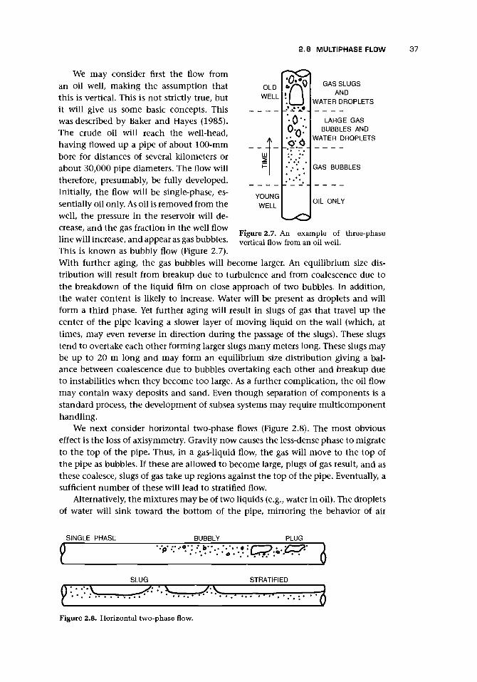
2.8 MULTIPHASE FLOW 37
OLDWELL
YOUNGWELL
a GAS SLUGSAND
WATER DROPLETS
LARGE GASBUBBLES AND
WATER DROPLETS
GAS BUBBLES
OIL ONLY
Figure 2.7. An example of three-phasevertical flow from an oil well.
We may consider first the flow froman oil well, making the assumption thatthis is vertical. This is not strictly true, butit will give us some basic concepts. Thiswas described by Baker and Hayes (1985).The crude oil will reach the well-head,having flowed up a pipe of about 100-mmbore for distances of several kilometers orabout 30,000 pipe diameters. The flow willtherefore, presumably, be fully developed.Initially, the flow will be single-phase, es-sentially oil only. As oil is removed from thewell, the pressure in the reservoir will de-crease, and the gas fraction in the well flowline will increase, and appear as gas bubbles.This is known as bubbly flow (Figure 2.7).With further aging, the gas bubbles will become larger. An equilibrium size dis-tribution will result from breakup due to turbulence and from coalescence due tothe breakdown of the liquid film on close approach of two bubbles. In addition,the water content is likely to increase. Water will be present as droplets and willform a third phase. Yet further aging will result in slugs of gas that travel up thecenter of the pipe leaving a slower layer of moving liquid on the wall (which, attimes, may even reverse in direction during the passage of the slugs). These slugstend to overtake each other forming larger slugs many meters long. These slugs maybe up to 20 m long and may form an equilibrium size distribution giving a bal-ance between coalescence due to bubbles overtaking each other and breakup dueto instabilities when they become too large. As a further complication, the oil flowmay contain waxy deposits and sand. Even though separation of components is astandard process, the development of subsea systems may require multicomponenthandling.
We next consider horizontal two-phase flows (Figure 2.8). The most obviouseffect is the loss of axisymmetry. Gravity now causes the less-dense phase to migrateto the top of the pipe. Thus, in a gas-liquid flow, the gas will move to the top ofthe pipe as bubbles. If these are allowed to become large, plugs of gas result, and asthese coalesce, slugs of gas take up regions against the top of the pipe. Eventually, asufficient number of these will lead to stratified flow.
Alternatively, the mixtures may be of two liquids (e.g., water in oil). The dropletsof water will sink toward the bottom of the pipe, mirroring the behavior of air
SINGLE PHASE BUBBLY PLUG
0 '• • 'V(
SLUG
•p-vr:
•
STRATIFIED
• . . . 0Figure 2.8. Horizontal two-phase flow.

38 FLUID MECHANICS ESSENTIALS
bubbles, and will eventually drop out onto the bottom of the pipe causing a contin-uous layer of water.
With a sufficient length of straight pipe (100D or more), a fully developed flowmay be achieved. However, in most applications we shall not be able to predict theresulting flow or how it will affect equipment in the line. This presents a considerablechallenge to the development of instrumentation for handling oil well flows in sub-sea installations. It may be possible to mix the fluid to create a more homogeneousfluid for flow measurement, but this will cause severe turbulence and a changingprofile, conditions generally considered unsuitable for such a measurement, not tomention the pressure loss which may result.
Liquids may contain gases in solution. For water, the maximum amount is about2% by volume. The gas in solution does not increase the volume of the liquid byan amount equal to its volume since the gas molecules "fit'' in the "gaps" in theliquid molecular structure. For hydrocarbons, the amount of gas that can be held insolution is very large, and the GOR (Gas-to-oil ratio), which is the volume of gas atstandard conditions to the volume of liquid, can range up to 100 or more. In eithercase, but particularly the latter, changes in flow conditions (e.g., a pressure drop)can cause the gas to come out of solution causing a two-phase flow with, possibly,severe effects on instrument precision.
In low head flows (e.g., in a sewage works), the flowing stream may entrain air,and a dispersion of air in water may result.
2.9 CAVITATION, HUMIDITY, DROPLETS, AND PARTICLES
Cavitation may occur in certain liquid flows at pressures around ambient. Cavitationis the creation of vapor cavities within the liquid caused by localized boiling at lowpressure. It can cause damage (e.g., in pumps, propellers, valves, and other flowcomponents) because the cavities can collapse very quickly with large, althoughlocalized, impacts and can erode solid surfaces. It can also cause errors in flowmeterreadings because it results in a larger volume than for the liquid alone.
High humidity may also create problems if it results in a consequent large amountof water vapor changing to liquid droplets in the gas (e.g., in critical flow venturinozzles).
Particulate matter can, in addition, cause wear and may need to be removed witha fine filter.
Much can be learned by computing the trajectories of droplets and particles (cf.Ahmad et al. 1986, Hayes 1988), and such an approach may be usefully applied toflowmeters. Droplets and particles will affect their performance in various ways.
a. They will cause flowmeters to read incorrectly, and most often this will be dueto the flowmeter responding to the volume flow of the gas phase and not fullyaccounting for the greater mass carried in solid and liquid.
b. They may cause erosion of the flowmeter body and sensing element.c. They may give false pulse readings in vortex flowmeters by hitting the pressure
sensor.d. They may become trapped in vortex structures around both stationary and mov-
ing parts of the meter.

2.11 STEAM 39
The basic flow around most meter internals is now predictable from standard com-puter programs, and a bubble/droplet/particle trajectory model should be combinedwith such a prediction. From such studies, it may be possible to design internals lesssusceptible to bubble/droplet/particle effects or to understand better the effects on,and to optimize the design of, meters such as the turbines described by Mark et al.(1990a, 1990b).
For electromagnetic and ultrasonic meters, further work on the interaction of thefield and bubble/droplet/particle may lead to more sophisticated sensors. Furtherstudy should also address the effect of large bubbles on the performance of suchmeters and on ways of flow-pattern mapping in general.
2.10 GAS ENTRAPMENT
Gas entrapment appears to occur in some flow geometries with important effects.Thomas et al. (1983) observed that 'Transient large eddies (vortices) in turbulentfree shear flows entrap and transport large quantities of bubbles, and may also forcethe coalescence of bubbles/' At the conference where this paper was presented, theappearance of this phenomenon was discussed in relation to two papers in particular,which suggested the presence of the phenomenon. In one of these, Baker and Deacon(1983) had tested a turbine meter that appeared to exhibit hysteresis in its responseto increasing and decreasing fractions of air in water. This may have been due to theparticular meter or the flow circuit, but it raised speculation as to whether vortexstructures in the vicinity of the ball bearing fluid access path could be entrapping airand holding it in the bearing after the external air content in the flow had dropped.Presumably such entrapment could occur in the vortex downstream of an orificeplate [Figure 2.9(a)].
Hulin and Foussat (1983) observed the entrapment of a second phase in the shedvortices behind a meter bluff body. Figure 2.9(b) shows a diagram of this mechanism.
I have also observed, in some field data from an ultrasonic flowmeter, a behaviorthat could result from entrapment of air. A meter in a low head flow, where air wasentrained with the water, periodically failed. The possibility that, in such a flow, thetransducer cavities could cause small local vortices which could entrap the air andblock the ultrasonic beam offered a possible explanation [Figure 2.9(c)].
There is considerable scope for investigating in other applications the appearanceof such entrapment and the likely effect. In flow measurement, entrapment may alsooccur around the throat of a Dall tube and behind an averaging pitot tube or otherprobes inserted in the flow. In all these cases, it is likely to affect the reading of theflowmeter. Entrapment may also occur in pumps, where it may reduce performance,and in pipework where abrupt area changes exist.
2.11 STEAM
One truly two-phase fluid is steam. Superheated steam may be treated as a gas, andits properties are well tabulated. However, it is increasingly important to measurethe flow of wet steam made up, say, of about 95% (by mass) vapor and about 5%
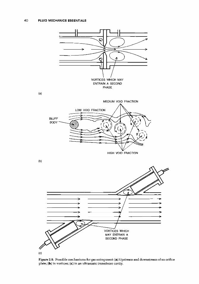
40 FLUID MECHANICS ESSENTIALS
(a)
VORTICES WHICH MAYENTRAIN A SECOND
PHASE
MEDIUM VOID FRACTION
LOW VOID FRACTION
HIGH VOID FRACTION
(b)
VORTICES WHICHMAY ENTRAIN ASECOND PHASE
Figure 2.9. Possible mechanisms for gas entrapment: (a) Upstream and downstream of an orificeplate; (b) in vortices; (c) in an ultrasonic transducer cavity.

2.12 CHAPTER CONCLUSIONS 41
liquid. The droplets of the liquid are carried by the vapor but will not follow thevapor stream precisely. As with water droplets in oil, the liquid will drop throughthe vapor to land on the pipe wall, and we may obtain an annular flow regime untilsufficient turbulence is created to reentrain this liquid. The measurement of such aflow causes major problems because the pressure and temperature remain constantwhile the dryness fraction changes. It is therefore not possible to deduce the drynessfraction or density from the pressure and temperature, and, in addition, the dropletsmay cause an error when we attempt to measure the flow.
Some pointers from the literature will be referred to in relation to some of thetypes of flowmeter. However, the best and safest advice is to use a water separatorupstream of the flowmeter and to measure the resulting flow of dry saturated steam.
2.12 CHAPTER CONCLUSIONS
I have been highly selective in choosing topics for inclusion in this chapter. Onceagain the reader is referred to fuller texts on fluid mechanics. Baker (1996) waswritten, particularly, with the industrial flowmeter user in mind and enlarges onsome of the points made in this chapter.
The development of computational fluid dynamics provides a tool for analyzingflowmeter behavior, and references will be mentioned in the other chapters. I con-sider that perturbation methods should be explored. These methods would allow agreater precision in defining performance change between the ideal flow through ameter and the disturbed flow due to turbulence change, profile distortion, or swirl.
The effects of small amounts of a second phase offer possibilities for investigatingthe behavior of particle/bubble/droplet in flows through meters by developing, forinstance, methods such as those of Ahmad et al. (1986) or Hayes (1988).
Work on flow conditioning is at present subject to thorough investigation byLaws and others as indicated, and Mottram and others continue to provide importantinsights into the effect of pulsating flows.
The critical flow venturi nozzle, as we shall see, appears to be capable of higherprecision than has been accepted. There may be value in fluid behavior investigationsin this and other areas to define ultimate limits of accuracy.

CHAPTER 3
Specification, Selection, and Audit
3.1 INTRODUCTION
The object of this chapter is to assist the reader in specifying a proposed flowmeter;soperational requirements as fully as possible and hence to enable the reader to selectthe right flowmeter. The reason for wishing to select a flowmeter may be obvious:a flow rate to be measured. However, the reason in some cases may be less obvious.If you are a flowmeter manufacturer, or prospective manufacturer, you may wishto identify a type and design that would meet a particular market niche. If youare a member of an R&D team, you may be exploring measurement areas that areinadequately covered at present.
In preparing this chapter, I have developed earlier ideas (Baker 1988/9, Bakerand Smith 1990), but I have also benefited from the ideas of others such as Endresset al. (1989). Baker (1988/9) was the best distillation I could offer in the late 1980s.There is much there that I would still endorse. In Baker and Smith (1990), we took adifferent line. We provided the means to specify the user's needs in as much detailas possible. We then provided a form for communication with the manufacturer.
Many people have attempted to provide a means of selecting a flowmeter. Aglance at only a few of the many books on flow measurement in the bibliography willindicate this. I used to feel that the way forward was to write an expert system to dothe job. I am less convinced about that now. One reason for this is that manufacturersappear to be extending the flowmeter types they offer and their applications, so thatkeeping the expert system up-to-date is a major task, and the decision on the bestmeter for a particular job may rest on more subtle considerations than an expertsystem is likely to include. This suggests that the expert system should narrow thefield pending the final choice in consultation with manufacturers or consultants.
I have picked out a few examples from the literature of application to specialistareas. This selection is not intended to be exhaustive but rather to complement theapplications identified for each flowmeter type in other chapters.
3.2 SPECIFYING THE APPLICATION
The change that I perceive over the last 10 years is that the main manufacturershave recognized the need to have within their armory a meter for every occasion. Insome cases, this has led to existing meters being applied to new and more demandingapplications. When I wrote Baker (1988/9), I was fairly skeptical as to the extent that
42
3.3 NOTES ON THE SPECIFICATION FORM 43
flowmeter types could be eliminated for particular applications. I am now more so.On a regular course at Cranfield University, we divide up into working groups inorder to select flowmeters for particular applications. Almost invariably there arethree or four meters suitable to a lesser or greater extent for each application.
I have, therefore, developed the theme of Baker and Smith (1990) in this chapter.We start with a form and discuss the implications of each item for user and manu-facturer. Before the reader turns to the form and concludes that it is unrealistic fora user or manufacturer to complete or respond to such a form, I would hasten todefend its inclusion because
i. it provides a check list of features that might otherwise be forgotten in specifyingthe meter, and
ii. it is there to be modified, simplified, and reduced in length and complexity, untilit suits individual needs.
The form is set out in Appendix 3.A.I under eight headings, which are labeledalphabetically. It can be photocopied and/or adapted. It is aimed at the user andcurrent manufacturer, but it should provide a starting point for the prospective man-ufacturer, who may wish to identify a type and design for a particular market niche,or for a member of an R&D team, which is exploring new development areas. Insummary the eight headings are:
A. General information about the meter manufacturerB. General description of the meter user's business and specific applicationC. Details of fluid to be measuredD. Site detailsE. Electrical and control detailsF. Other user information such as preferred accuracy, materials, maintenance, and
cleaningG. Manufacturer's additional information and requirements such as warranty,
filtration requirements, and priceH. Other considerations and final conclusion
The audit of a flowmeter should link closely with the specification and selection.To ensure consistency, the final section on audit reverts to the specification tableand reviews the correctness of the original assessment (if there was one) or theappropriateness of the selection.
3.3 NOTES ON THE SPECIFICATION FORM
A INFORMATION ABOUT THE MANUFACTURER
In approaching a manufacturer, it is important to know whether it will want to sellyou its one and only flowmeter type - however appropriate or inappropriate foryour application - or whether it has a range of meters, which will ensure that oneis appropriate to your needs. It is also useful to know how many the manufacturersells and the satisfaction of other customers. A manufacturer may be wise to include

44 SPECIFICATION, SELECTION, AND AUDIT
illustrations of a high quality production line in its literature as well as indicationsof its international sales and servicing structure.
In making this point, I have no intention of excluding the smaller high qualitymanufacturer whose products will be sold on their special features and adaptability.Such a manufacturer will have its own strengths. Indeed, the manufacturer shouldbe clear as to what they are and base its selling strategy on them. In fact, many, if notmost, manufacturers' outlets in a particular country will fall in the category of smalland medium-sized enterprises (SME) and are likely to give a personalized service.
B USER'S BUSINESS AND SPECIFIC APPLICATION
The object of this section is to provide the manufacturer with a clear overview ofthe application, site, and essential background to maintenance and safety on site.
The relevant safety documents and those dealing with other relevant standardsand legislation on electromagnetic compatibility (EMC) should be referred to (notethe CE marking requirement in Europe). Endress et al. (1989) provides a useful digestof the safety requirements for Europe and the United States.
C FLUID DETAILS
The user should endeavor to provide the manufacturer with the fullest informationpossible to avoid any incompatibility between fluid and meter. Of those propertiesrequested, conductivity only applies to liquids where an electromagnetic flowmeteris to be considered. Opacity would be relevant only for meters that use optical sensingthrough the fluid. Compressibility may relate to the behavior of differential pressureand ultrasonic flowmeters, and it may be useful for the manufacturer in advising onsuch applications.
Lubricity has not been included in the list. On the basis of definitions in dic-tionaries and encyclopedias, lubricity may be taken to mean boundary lubricatingproperties.* It is a term frequently used in the flowmeter business, where the mea-sured fluid is often expected to act as lubricant for the flowmeter rotor. Lubricitygenerally is used to indicate the ability of the metered fluid to lubricate the bearingsof a rotating meter insert.
Lubricity does not appear to be a term used by lubrication experts. Its meaningwould seem to be related to the high friction coefficient in a lubricated bearing atlow viscosity. This is best illustrated by the Stribeck diagram, Figure 3.1 (a) (fromSummers-Smith 1994). This shows that as the viscosity n or rotational speed n of thebearing decreases or the load p increases, the friction coefficient r\ falls to a certainpoint. In this region, hydrodynamic lubrication occurs, and the curve has a positiveand fairly constant slope. Following this for smaller values of viscosity, the curve has asharp negative slope. Where the curve meets the vertical axis, boundary lubricationtakes place as the surfaces come into contact. This is matched by a curve with asimilar shape [Figure 3.1(b)] which shows the friction coefficient r\ as a function ofthe specific film thickness X, the ratio of the lubrication film thickness hmin, and thecombined roughness of the two contacting surfaces a. The minimum occurs (region
Private communication from J. D. Summers-Smith.

3.3 NOTES ON THE SPECIFICATION FORM 45
11
1.0
0.1
0.01
0.001
0.1
0.01
0.001
-
-
Ai
\
\
\
Bi
C Di
\inlp 0.1 10 100
(a) (b)
Figure 3.1. Friction variation (from Summers-Smith 1994; reproduced with permission of theauthor and Professional Engineering Publishing): (a) Stribeck diagram for a journal bearing;(b) Coefficient of friction as a function of specific film thickness.
C) where the clearance is slightly larger than the surface roughness dimension, andthe rapid increase in friction coefficient with decreasing viscosity occurs (region B)due to the smallness of the clearance allowing interference between the roughnesson the opposing faces.
It, therefore, seems likely that low lubricity has been used to refer to situationswhere /Jin/p is very small, where /x is fluid viscosity, n is rotational speed, and p is load.Many gases will require external lubrication in turbine meters, whereas a bearinglessflowmeter may be suitable for hydrofluoric acid and very dry liquids such as carbondisulfide.
Some gases (e.g., oxygen) require special lubrication. Because it oxidizes steelpipes with the danger of chunks of rust detaching from the pipe wall, a maximumvelocity is sometimes specified for oxygen flows.
Abrasiveness caused by solids in the flow will clearly be a problem for bearingsand will lead to wear unless the particulate matter is filtered out.
D SITE DETAILS
Much of the data requested would be clarified and reinforced by a site plan. Detailsof access and environmental hazards are clearly essential. The access may be suchthat the meter has to be man-handled into position, placing severe limitations onweight.
E ELECTRICAL AND CONTROL DETAILS
Whether the proposed instrument becomes part of a sophisticated modern telemetrysystem or is a stand-alone with local power - not to mention all the intermediatevariants - will make a lot of difference to meter specification. In addition, all safetydetails for the site must be set out either here or under environmental hazards in D.Appropriate documents on safety should be consulted.
F OTHER USER INFORMATION
In specifying accuracy, it is essential that the user does not overstate requirements orthat the manufacturer does not oversell the product. The accuracy should be realisticwhen the total installation constraints are taken into account. Response time should

46 SPECIFICATION, SELECTION, AND AUDIT
be appropriate to the requirements of the plant. For a plant with, say, a dosing periodof 10 s, the response will need to be rapid enough to achieve the required dosingprecision. The instrument identified by the manufacturer should fit in with existingplant schedules as far as possible and should be compatible with extreme conditions(e.g., steam cleaning of hygienic process plant).
G MANUFACTURER'S PROPOSED METER AND REQUIREMENTS
This section allows the manufacturer to specify the meter that most nearly meetsthe user's requirements. The manufacturer should make clear any ways in which themeter will not meet the specification. The details of the calibration procedure forthe flowmeter should be spelled out.
The form may well have been supplied to several manufacturers, and this sectionwill provide the user with a comparison of the possibilities.
H ANY OTHER CONSIDERATIONS AND CONCLUSIONS
This is an opportunity for the manufacturer to add further information and for theuser to summarize the decision on selection.
3.4 FLOWMETER SELECTION SUMMARY TABLES
Table 3.1 is an update of the table in Baker (1988/9) resulting from the fuller infor-mation included in this book. It lists the main types of flowmeter as set out in thechapters of this book and attempts to encapsulate the key features.
For convenience, they are subdivided into momentum-, volume-, and mass-sensing meters. This subdivision also emphasizes that, for instance, a meter respond-ing to momentum will be sensitive to density change. Where a less common meterof the same family has particular features that make it unique or particularly use-ful in certain applications, these may be indicated in notes in the table and in thediscussion in subsequent chapters, where other points arising from this chapter willbe elaborated. This table, therefore, provides a first cut at the selection for the taskwhich has been identified by the specification questionnaire. The values given aremy best estimates at the time of writing, but they probably fail to reflect the inherentvariation in designs.
Nature of the Fluid to Be MeteredThe first choice, liquid or gas, will cause a few types of meters to be eliminated. Theselection of suitable meters for slurries and two (or more)-phase flows, is severelyrestricted at present. In Table 3.1, X indicates unsuitable, and * indicates suitableexcept where some are more suitable (**) than others. A ? indicates that it is notcohimon but might be appropriate in this application. The electromagnetic flow-meter has found a valuable role in slurry flow measurement. However, the Coriolismass flowmeter is sometimes claimed to be suitable for slurry, and an ultrasonic flow-meter has been specially designed for this purpose. The electromagnetic flowmeter isalso useful in two-phase flows when the continuous phase is conducting. However,Venturis are usable, but with caution. The ultrasonic correlation flowmeter and thedoppler flow monitor may also be worth considering in such flows.

3.4 FLOWMETER SELECTION SUMMARY TABLES 47
Flowmeters with rotating parts will be less suitable for dirty abrasive fluids or forfluids that do not lubricate adequately. Abrasion may also detract from the perfor-mance of meters, such as the vortex meter. Cavitation should be avoided. The liquidmust be conducting for current commercial electromagnetic flowmeters.
Flowmeter Range and SpecificationAccuracy is perhaps the most difficult to determine because both user and manu-facturer are prone to overstate their requirements and capabilities. In Table 3.1,
***is for random error < 0.1% rate,**is for random error < 0.5% rate, and*is for random error < 2% rate.
The estimates reflect my view of the accuracy of flowmeters. These values shouldbe achievable with a particular type of flowmeter. For a standard orifice the uncer-tainty before calibration due to the discharge coefficient is 0.5-0.75%, and overalluncertainty will be greater than this when errors in the measurement of dimensions,pressure, and density are included. After calibration, the total uncertainty will be lessthan this, and it is reasonable to assume that the random error will be less than 0.5%.This appears to be confirmed by data. Some manufacturers may feel able to claimhigher values for the various meters than those in the table, but the reader shouldask for justification for such claims. Commercial flowmeter claims of better than0.5% indicate a level of accuracy that is probably only achieved in a few designs.Some manufacturers may not always achieve the values indicated. The repeatabilityof a variable area meter is often quoted as a percentage of full scale, and so may bejust outside the * rating for flow rates over, say, the top half of the range.
Precision relates to random error. It does not allow for changes in bias errorcaused by changes in method of measurement, location, or long elapsed times. Thus,if the reader is concerned about long-term repeatability or total uncertainty, theseestimates may not provide the most appropriate guide.
Diameter, temperature, and flow are my best estimates based on manufacturers'literature. In all cases, the diligent reader can probably find examples of greater rangesthan those given, and manufacturers are always seeking to extend the capability oftheir instruments. Note that, in the column for flow range, the values in parenthesesindicate kilograms per hour rather than cubic meters per hour.
The maximum pressure has not been included because, apart from exceptionallyhigh pressure applications, when one might turn to an orifice plate or a turbine me-ter, there appear to be versions of most designs that are offered for normal industrialranges. In some cases, minimum pressures maybe important because cavitation maybe a danger, and the manufacturer should be consulted.
The pressure loss is given as H (high), M (medium), or L (low). Only meters witha clear bore have been categorized as L because there is virtually no more pressureloss than in a similar length of pipe. The orifice plate meter is H/M, and positivedisplacement meter and vortex are H/M, although their relative losses will dependon such things as the instrumentation being driven by the positive displacementmeter.

48 49
Table 3.1. Flowmeter selection summary tables
1Flowmetertype
Momentum"Orifice
Venturi
Nozzles
Variable-area
OtherVenturi-like
Averagingpitots
Laminar
VolumePositive
displacement
Turbine
Vortex
Electromagnetic
Transit-timeU.S.
MassMultisensorWheatstone
bridge
Thermal
Angular mom.
Coriolis
2Liquidor Gas
LG
LGLGLGLGLGG
LG
LG
LGL
L
G
LL
LGL
LG
Key: ***, Very high; **,
3 4 5 6Other Typical
Slurry Two-Phase Accuracy Turndown'*
X ? ** 5:15:1
5:1** 5:1
? * ** 5:1*' 5:1
X X 10:110:1
? ? ? 3:13:1
X X ? 10:110:1
X X ? 20:1
Xb Xb . * . 1 0 ; 1
*** 80:1
X X *** 10:1*** 30:1
X X ** 20:1** 20:1
** ** •• 100:1
•fb -fb « • 20:1
** 30:1
X X ** 50:1
X X * 15:1* 50:1
X X * 7:1
* X ** 100:1* *
More suitable/high; *, Suitable/medium
7Diae
Range (mm)
50-1,00050-1,000
50-1,20050-1,20050-63050-63015-15015-15013-1,20013-1,20025-12,00025-12,000?
4-200
5-60025-600
12-20012-2002-3,000
10-2,000
20-1,000
?6-60
2-66-200
20-50
6-200
8Temp fRange (°C)
-200 to 350
up to 450-100 to 450
-50 to 290-40 to 65
-265 to 310-10 to 50
-200 to 400
-50 to 190
-200 to 260
-50 to 260
?-18 to 150
0to65-50 to 300-40 to 150
-240 to 200
9Flow Ranged(m3/h (kg*))
1-3 x10⁵
10-4 x 10⁶
30-7,000400-105
2-1.7 x 10⁴
20-2.5 x 10⁵
io-4-ioo10-2-2,000
10-3 x 10"200-6 x 10⁵
up to 120
0.01-2,0000.01-1,200
0.03-70000.01-25,000
3-2,00050-104
10"2-105
3-105
0.04-105
(0.05-2.3 x 10⁴)
(0.002-100)(2 x 10~4-8000)(100-4.5 x 10³)
(1-7 x 10⁵)
10 11Pressure Sensitivity toLoss
H
M
M
M
L
H
H/M
M
H/M
L
L
H?
ML/MM
M/L
; ?/blank, Uncertain/lower; X. Unsuitable. L =" Some proprietary devices offer special features: higher differential pressure
Some designs have been produced for slurries.c Multisensor systems have been developed specially for multiphase.d Typical estimates thate Larger or smaller sizes
;, linear characteristics.
Installation*
H/M
M
H/M
L/M
H/M
H
L
L
H
H/M
M
H/M
H/M
L
L(CTMF)M/H(ITMF)M
L
rmmmm
12InitialCost
L/M
M/H
M
L
M/H
L
M
H/M
L/M
L/M
M
M/H
M/H
HH
M
M
H
Notes
Concentric ISO orificewith differential pressurecell assumed
Does not include criticalnozzle.
Glass/plastic assumed;higher ratings for steel.
Consult manufacturers.
Particularly appropriatefor pulsating flows.
Turndown given may beachieved for rotary positivedisplacement gas meter.
High precision instrumentsassumed rather thanwater meters, etc.
Fluidic flowmeter suitable forwide range of utility flows
Only available commerciallyfor conducting liquids.
Single beam are moresensitive to installation.
Correlation and dopplerfor two-phase flows.
Specialist instrumentespecially for enginetesting.
Higher flows require CTFMwith bypass or ITMF.
Particularly suitablefor aircraft fuel flow.
Straight single tube hasessentially zero pressuredrop. Gas ranges areprobably more limited.
= Low; M = Medium; H = High.
may be exceeded by using smart transducers and may be greater or less than the value attained by some designs.may be available.
f Other ranges may be available.* Flow conditioning may be used in some applications to reduce this effect.
J

50 51
Table 3.2. Rough selection criteria for liquid and gas flowmeters'• Property of liquid
' Clean • • • • • • • • •Slightly contaminated • • • • • • • • •
-* Contaminated or abrasive • • • • • • • • •Heavily contaminated • • • • • • • • •Viscosity below 10 cSt • • • • • • • • • • • •Viscosity 10 to 40 cSt • • • • • • • • • • • •Viscosity over 40 cSt • • • • • • • • • • • •
Diameter
<25 mm (<1 inch) • • • • • • • • • • • •25 to 500 mm (1 to 20 inches) • • • • • • • • • • • •
• > 500 mm (> 20 inches) • • • • • • • • • • • •
' Type of flowmeter
Magnetic" • • / / • / / / / / / • • • / • • • • • / / / / • / • • • • • • • / / /Mass flowmeter / / / / / / / / • • • / o o o o o oVortex • o / O / o / O • o / OUltrasonic transit time / / / / / /Differential pressure 0 0 0 / / / / / / 0 0 0 / / / / / / 0 0 0 0 0 0 0 0 0Positive displacement / / / / / /Variable area / / / / / / / /Turbines / / / / / / / • • • • •Property of gas
Clean • • • • • • • • •Slightly contaminated • • • • • • • • •Contaminated • • • • • • • • •
'. High humidity • • • • • • • • •Density >60 kg/m3 (3.75 lb/ft3) • • • • • • • • • • • •Density 1 to 60 kg/m3 • • • • • • • • • • • •
(0.06 to 3.75 lb/ft3)- Density <lkg/m3 (0.06 lb/ft3) • • • • • • • • • • • •
Diameter
> <25 mm (<1 inch) • • • • • • • • • • • •. 25 to 500 mm (1 to 20 inches) • • • • • • • • • • • •
>500 mm (>20 inches) • • • • • • • • • • • •
Type of flowmeter
Vortex* / / o / / o / / o / / o• Differential pressure 0 0 0 / / / / / / 0 0 0 / / / / / / 0 0 0 0 0 0 0 0 0 0 0 0 0 0 0 0 0 0
Positive displacement / / / / / /1 Variable area / • / / / / / / / / / /
Turbines / / 0 / / 0 / / 0 / / 0 O O O O
• Reproduced from Endress et al. (1989) with permission.i Key: o = only under special conditions (e.g., special version, only certain diameters); • = Property of material; •" = suitable.* " Only if liquid is electrically conductive.; b Suitable for steam measurement.1

52 SPECIFICATION, SELECTION, AND AUDIT
Installation effects caused by upstream pipework will be a recurring theme inmost chapters. The positive displacement meter may be assumed to be insensitive toupstream installation effects and is, therefore, rated L. A few others, also, have lowsensitivity to installation. However, most flowmeters are affected, and these havebeen categorized for a fitting, such as a bend, at 5D upstream.
L, negligible effect;M, <2% increase in uncertainty;H, >2% increase in uncertainty.
These categorizations are my best estimates, and manufacturers may be prepared touprate them.
Most flowmeters are sensitive to pulsation over part of their range, with thepossible exception of the ultrasonic flowmeter and the laminar flowmeter, whichwas specially designed to cope with pulsating gas flows.
The flowmeters with essentially a clear straight bore (nonintrusive) are the elec-tromagnetic, ultrasonic, and some Coriolis designs. The only flowmeter that mayfail and block the line is the positive displacement flowmeter. All the others havepartial line blockage, although the venturi has such a smooth change in section thatits effect is probably of small concern.
Only the ultrasonic family offers clamp-on options (noninvasive) at present.Response time will depend on fluid inertia, component inertia, or electrical
damping. The first two are inherent to the meter type and are not reducible. Theelectrical response may be speeded up in some meters provided stability and noisepermit.
The installation of the flowmeter will also be affected by environmentalconsiderations, such as ambient temperature, humidity, exposure to weather, elec-tromagnetic radiation, and vibration. These will need to be assessed in consultationwith particular manufacturers. The area safety and explosion classification shouldalso be checked.
Price and CostThis is possibly the most important consideration and is difficult to tabulate becausethe range of price for any design is wide and the data are always changing! Therefore,I have attempted to rate the initial cost of the flowmeters as H (high), M (medium),or L (low). However, the medium bracket tends to become a "catch-all" and covers,for instance, electromagnetic and turbine flowmeters, which can actually have aninitial cost range of 4:1 for a 100-mm diameter design. For this reason, L/M or M/Hhave been used where low or high cost versions are available.
Initial cost will, of course, include both purchase price and cost of installation.There will also be ongoing costs associated with maintenance, energy loss due to thepresence of the flowmeter, and savings based on the information provided by theflowmeter. If the flowmeter is clearly required, then the savings should outweigh thecosts. This does not reduce the responsibility of the user to install the best and mosteconomical instrument for the job!
Table 3.2 is reproduced with permission from Endress et al. (1989) and gives arough guide to the flowmeters most likely to be useful, but starting with the natureof the fluid and the pipe size.

3.5 OTHER GUIDES TO SELECTION AND SPECIFIC APPLICATIONS 53
3.5 OTHER GUIDES TO SELECTION AND SPECIFIC APPLICATIONS
General Selection AdviceApart from my introductory guide (Baker 1988/9), the reader is referred to the BritishStandard Guide (BS 7405:1991) to the Selection and Application of Flowmeters for areview of each type of flowmeter and a guide to selection (cf. Furness's 1991 review ofBS 7405). Miller (1996) offers some guidance on selection, as does Hayward (1979),which is still good value, even if a bit dated. The Institute of Petroleum guide (IoP1982) gives a comprehensive list of information required.
Furness and Heritage (1989) gave a breakdown of considerations when selectinga flowmeter, similar to those in the British Standard. In particular, they have usedthe 11 categories of meter type set out in the Standard, although slightly modifiedto include open channel flow measurement. This is an interesting subdivision, butit is not one I have chosen to use in this book. A useful aspect of the directory is itsability to provide the names of all flowmeter manufacturers. However, the nameschange with great rapidity in this field, as company buy-outs take place.
A review of flowmeters by Ginesi (1991) covers well-trodden ground, but it alsois a reminder that some less common meters (e.g., the segmental wedge flowmeteror the V-cone) may offer solutions.
Refinery Flow MeasurementFurness and Jelffs (1991) sought to make a case for using meters to measure flowsin and out of refineries rather than depending on tank transfer. They also mentionbriefly some problems in flow metering.
• For gas metering, the gas often contains liquid.• Provided there are no liquid particles, the orifice plate should retain its sharpness,
although they suggest that these meters seldom achieve an accuracy of betterthan 4%.
• Flare gas metering poses problems of large turndown.• Rotating meters are usually unsuitable for naphtha because external lubrication
is necessary.• Black oils require positive displacement meters with heavy-duty rotors and large
clearances, possibly with heat tracing.• On-line density measurement (they claimed) had a minimum uncertainty of
±0.3-0.5%.• Most Coriolis meters (they claimed) are influenced by density in a way that can
be checked only by proving gravimetrically, and the measurement within themeter of density is not sufficiently accurate to use a compact prover to obtain a±0.2% requirement.
They also refer to Shewhart Control Charts, which plot meter factor againsttime, with limits to indicate change that requires action by the plant staff; MovingAverage Charts, which detect long-term meter factor drift; and Cumulative Sum(CUSUM) Charts, which indicate the occurrence of an event due to some assignablecause.

54 SPECIFICATION, SELECTION, AND AUDIT
Water IndustryFowles (1994) commented that the selection of an instrument for a required duty is avery complex decision-making process. If the wrong selection is made, it can resultin abortive cost, erroneous information, and incoherent operational decisions. Inaddressing these problems, the user is often directed to American, British, European,and international standards. However, such specifications are often not suited to thespecific and often unique demands of the industry.
Reynolds (1994) discussed water industry specifications that have led to datasheets on electromagnetic, ultrasonic, differential pressure, insertion flowmeters,and ultrasonic level instruments. The data sheets consist, first, of technical specifi-cation and option selection to be completed by the purchaser and, second, supplier-provided information that will influence cost of ownership. A European set of in-strument specifications is also being established.
Nuclear IndustryFinlayson (1992) gave information on the use of flowmeters at one plant, which had1,500 flow measurements:
For Radioactive For Nonradioactive
Type Liquid Gas Liquid Gas
Electromagnetic / /Ultrasonic / /Differential pressure / / / /Variable area / /Turbine / / /Positive displacement /
For differential pressure, the paper gave diagrams of traps, vents, etc., and listed anumber of considerations.
• Stainless steel should be used for corrosive fluids and when behind shielding.• All welded construction should be used to avoid leakage.• All vents should be routed to a suitable drain for safety.• Drain legs should take the shortest route and be valved before penetrating plant
shielding.• Sensors should be housed in a shield bulge or a glove box.• Drain cocks within a shield bulge should have extended spindles to the outside
of the bulge.• Transmitters should be located outside the bulge or glove box in a lockable en-
closure or equipment room.
The paper described some of the flowmeters and modifications needed for the ap-plication, including a time-of-flight ultrasonic one.
Cryogenic ApplicationsRivetti and Martini (1990) reviewed various types of flowmeters for space applica-tions and concluded that only in a few cases were they suitable for cryogenic service

3.7 FINAL COMMENTS 55
and that, even then, care needed to be taken over the use of materials and the sen-sors. The use of superfluid helium for space applications required new approaches.They discussed specifically designed transducers of small size and weight with goodaccuracy and reliability. Thermal transducers and turbine meters that used super-conducting magnet suspension for the bearings appeared to be the most promising,although much work still remains to be done.
3.6 DRAFT QUESTIONNAIRE FOR FLOWMETER AUDIT
In this chapter we have taken a detailed look at the questions that a user and a manu-facturer need to answer before selecting a flowmeter for a particular application. Wehave then looked at two selection tables, which do little more than indicate therange of possible alternatives for most applications. We have also reviewed somepublished guidance.
This final section sets out the essential information needed if the flowmeter in-stalled is to be audited in the future. The objectives of such an audit should probablyestablish one or more of the following:
• The suitability of the flowmeter for the task,• The current state of the meter,• The optimum specification for a new flowmeter, and• The suitability of the flowmeter;s position for precise measurement and main-
tenance.
If in situ calibration is to be used, then the options need to be considered. The listin Appendix 3.A.2, based on Baker and Smith (1990), offers a starting point for theflowmeter owner. The list should be used either with the specification questionnaireif such exists or to create such a questionnaire for future meter actions.
3.7 FINAL COMMENTS
To the company that uses flowmeters, note that the results of auditing flowmetersmay vary widely. The replacement of meters because of age, wear, or incorrect sizingmay result in more precise measurements provided installation constraints allow it.However, this may not mean that the user reduces costs because correct measurementmay mean higher costs. One is tempted to suggest that, for statistical reasons, theoverall gain will be hardly worth the cost of the audit and replacement exercise. Ofcourse, the need for greater accuracy will exist if an absolute flow rate is needed forcontrol or fiscal reasons.
To the person responsible for purchase, make sure that you have specified therequirements carefully, and do not be content until you are sure that you have founda commercial device that matches your requirements in all points.
To the manufacturer, make sure that you have a clear understanding of thefollowing:
a. what you are offering and why it is superior to your competitors' designs;

56 SPECIFICATION, SELECTION, AND AUDIT
b. whether you expect to sell your products because you can offer a completerange for 95% of applications, or because you have the only device for particularapplications;
c. the weaknesses in your products that need to be addressed and the gaps in yourrange that need to be filled.
To the research center, identify the applications that have not been met and thetechnology most likely to meet them.
To the inventor, start from the application problem, look for features that may beinherently flow-dependent, and see if they can be used as the basis for a flowmeter.Remember that the power of modern signal processing should allow the mechanicaldesign to be very simple.
The development of an expert system to satisfy all parties would clearly be valu-able, but its production and updating may cost too much to make it worthwhile. Ishould like to prove myself wrong about this one day.
APPENDIX 3.A
Specification and Audit Questionnaires
3.A.1 SPECIFICATION QUESTIONNAIRE
ResponseA Information about the manufacturerAl Manufacturer and addressA2 Contact person and position in companyA3 Company size and international standingA4 Flow product range and turnoverA5 Other productsA6 Accreditation (BS 5750, ISO 9000, UK NAMAS, etc.)B User's business and specific applicationBl Company's site addressB2 Contact person and position in companyB3 General description of application and telemetry linksB4 Site safety requirementsB5 Current general policy on instrument maintenanceC Fluid detailsCl Chemical composition, state (gas or liquid), and materials that
are incompatible with the chemicalC2 Purity of chemical and if contaminated or multicomponent,
the nature of other components, likelihood ofdeposition
C3 Commonly known propertiesC3.1 DensityC3.2 Viscosity (if non-Newtonian, state type)C3.3 Conductivity

3.A.1 SPECIFICATION QUESTIONNAIRE 57
ResponseC4 Other features if known
C4.1 AbrasivenessC4.2 OpacityC4.3 CompressibilityC4.4 Flammability and other safety considerations
D Site details (a site plan should be attached if possible)Dl Flow range: maximum
minimumnormal flowlikelihood and size of over-range flows
D2 Pipework (a diagram should be attached if possibleextending to at least 50D upstream, particularly in caseswhere there are fittings that create swirl)D2.1 Outside diameterD2.2 Inside diameterD2.3 Material of pipe and pipe lining if presentD2.4 Flange size and details or other connection methodD2.5 Nearest upstream pipe fittingD2.6 Distance to upstream fittingD2.7 Distance to nearest downstream fittingD2.8 Orientation of pipe run
D3 Environment, etc.D3.1 Hazards including required safety and explosion-proof
classificationD3.2 Access, size, and weight limitations including
vehicle access, machinery transport, and shelterD3.3 Flow source (gravity, pumped, etc.)D3.4 Flow stabilityD3.5 Mounting requirements (including maximum weight)D3.6 Ambient working pressure: maximum
minimumnormal
D3.7 Fluid working pressure: maximumminimumnormal
D3.8 Ambient working temperature: maximumminimumnormal
D3.9 Fluid working temperature: maximumminimumnormal
D3.10 Maximum acceptable pressure dropD3.ll Electromagnetic and radio frequency interference at site
E Electrical and control detailsEl Overall control system in use with communication protocol
detailsE2 Power supply availability and variability

58 SPECIFICATION, SELECTION, AND AUDIT
ResponseE3 Preferred signal transmission if not defined previously:
0-20 mA4-20 mA0-1 kHz0-10 kHzPulse output: frequency range
pulse sizeDigitalOther
E4 Failure system:fail soft one operating and one stand-by channelfail passive two operating channelsfail operational three operating channels and one
decision elementfail safe output goes to safe condition
E5 Interelement protection (IP) given by IP XYX has range 0-6 for protection against access of foreign
bodies (Endress et al. 1989)Y has range 0-8 for protection against ingress of water
(Endress et al. 1989)F Other user informationFl Accuracy: uncertainty
repeatabilityF2 Response timeF3 Preferred construction materialsF4 Existing instrument maintenance schedulesF5 Line cleaning arrangementsG Manufacturer's proposed meter and requirementsGl Manufacturer's proposed meter specificationG2 Special requirements resulting from this proposal (e.g.,
filtration, power supply, environment)G3 Calibration details, rig conditions, and resultsG4 Warranty period and conditionsG5 DeliveryG6 PriceH Any other considerations and conclusionsHI Considerations and constraints by the manufacturer not
covered elsewhereH2 Agreement of the user to the proposed meterH3 Conclusion and decision
3.A.2 SUPPLEMENTARY AUDIT QUESTIONNAIRE
This questionnaire should be read in conjunction with the specification question-naire in Appendix 3.A.I.

3.A.2 SUPPLEMENTARY AUDIT QUESTIONNAIRE 59
AnswerA Information about the manufacturer
Not relevantB User's business and specific application
If the auditor is not part of the user's company, thenthis section may usefully be completed.
C Fluid detailsIs the meter of suitable design, construction, and
materials for this fluid?D Site details (Is the site plan correct?)
On the plan, mark power and signal cables and the position ofthe main meter electronics.
What is the meter power consumption?What is the flow range?Are these within the meter specification?
PipeworkIs the site of the meter satisfactory? If not, shouldmeter be moved?
Environment, etc.Is the meter suitable for this environment?Is meter design suitable for these hazards?Is the meter capable of operating within these
parameters?Is access sufficient for proper maintenance?
E Electrical and control detailsDo power, control, and signal systems match requirements
for operating and protection?Is there power and system access for audit and
maintenance work?What is the signal level?Is the meter permanently energized and if not what is
the warm-up procedure?What is the control system for the meter?Are there special: alarms?
low flow cutoffs?F Other user information
Has the meter accuracy been checked? If so, whatis the uncertainty? repeatability?
What are the materials of the meter? Do they match preferredconstruction materials?
Have instrument maintenance schedules been adhered to?If so, are there any apparent operational changes or
peculiarities that may have caused problems etc.?Has the meter reading changed unexpectedly?
What are the line-cleaning arrangements?

60 SPECIFICATION, SELECTION, AND AUDIT
AnswerG Manufacturer's information and requirements
Meter specification:Manufacturer?Type?Model?Serial number?Specification?
Where specification is unavailable, obtain key detailsas far as possible.
Expected accuracy?Construction date?Installation date?Subsequent checking/calibration/maintenance?Is documentation available? If so, list.
Are all special requirements met (e.g., filtration, powersupply, environment)?
Has the meter met the expected accuracy? If not, was itunrealistic/unnecessarily stringent?
H Any other considerations and conclusionsActions resulting from this audit?

CHAPTER 4
Calibration
4.1 INTRODUCTION
The object of calibration is to benchmark a flowmeter to an absolute datum. Justas a benchmark tells us how a particular geographical point compares in heightwith sea level datum, so a calibration of a flowmeter tells us how the signal fromthe flowmeter compares with the absolute standard of a national laboratory. Theanalogy is not perfect at this stage. The national laboratory standard must also becompared with other more fundamental measures of time and mass, and it will beessential to check and compare different national standards in different countriesfrom time to time.
There is a desire to reference back to fundamental measurements such as mass,length, and time. Thus if we can measure mass flow on a calibration facility byusing fundamental measurements of mass and time, this will bring us nearer tothe absolute values than, say, obtaining the volume of a calibration vessel by usingweighed volumes of water and deducing the volume from the density. The firstis more correctly termed primary calibration, whereas the second fails strictly toachieve this. It is likely that the final accuracy will reflect this. Liquid calibrationfacilities can achieve a rather higher accuracy than is possible for most of the gascalibration facilities. In part, this difference will result from the lower density andthe increased difficulties of handling a gas.
The result of a calibration will be both a comparison with the national standardand also a range within which the reading is likely to lie.
4.1.1 CALIBRATION CONSIDERATIONS
Figure 4.1 shows three different approaches to obtaining the data. Although theselection of calibration points and their optimum distribution over the range is notobvious, most of the reference books seem to omit any comment on this. Figure4.1 (a) records data at one flow rate. This might be appropriate if the flowmeter wereexpected to operate at one rate. It shows the fact that there is variation with time towhich the repeatability refers. Such a plot might be used to compare the calibrationfacility itself with other facilities or to test the consistency of diverter operation.Figure 4.1(b) is probably the most usual plot. Here a number of points have beentaken over the full range of the flowmeter. Figure 4.1 (c) shows a characteristic that hasbeen investigated in four positions, and three readings have been obtained in each.
The number of points will depend on the confidence of the user in the calibrationfacility, the quality and linearity of the flowmeter, and the statistical requirements for
61

62 CALIBRATION
(a)
ERROR INMEASUREDQUANTITY
SET•FLOW
RATE
(b)
TIME AFTER- H 1 1 1 1 1 1 1 1 1 1 1 1 1 START OF
START CALIBRATIONTIME
ERROR INMEASUREDQUANTITY
x x , FLOWl~~~ RATE
10%
ERROR INMEASUREDQUANTITY
10% 50% 100%
FLOWRATE
(c)
Figure 4.1. Diagram to show different calibration plots, (a) Measurements at a constant flow ratetaken over a short period of time, (b) Measurements of the full characteristic of the flowmeter.(c) Measurements repeated at certain points in the flowmeter characteristic.
the required confidence level. Thus a manufacturer may have sufficient confidencein the quality of manufacture of its products to use, say, just two calibration points,and three readings might be taken for each to guard against one spurious reading. Itmight then be justified in claiming a ±1% envelope for its product. This is unlikelyto be a nationally accredited calibration. On the other hand, 20 points or more alonga complete characteristic of adequate linearity may be needed to ensure, for a high

4.1 INTRODUCTION 63
quality meter, an acceptable value of uncertainty. At any point on the characteristic,there will need to be sufficient neighboring points to achieve the required confidencelevel. (See Section 1.A.4 where there is such a calculation.)
Ideally the flowmeter would be calibrated under conditions identical with serviceones. In practice, in situ calibration is not very accurate, and a calibration facilitywill provide the reference conditions for an instrument given that installation andother influence conditions will increase the uncertainty. We shall therefore wish toconsider the following factors.
Fluid: If the service fluid is water, then we shall have few problems, althoughit will still be necessary at least to check for gas in solution, for purity, and fortemperature. However, if the fluid is anything else, there will be a range of decisions.If we cannot match the fluid perfectly, we shall add to the final uncertainty of thecalibration because the effect of, say, calibrating a meter for oxygen service on air willrequire a calibration adjustment. This adjustment will, itself, have an uncertaintyin it.
Flow Range: It is obviously preferable if this is identical to that for the service.However, if the fluid conditions are not identical, then there may be a compromisebetween velocity through meter, mass/volumetric flow through meter, and Reynoldsnumber. If the fluid for calibration differs from the fluid for service, the differingviscosity may cause the Reynolds numbers not to match. The importance of this isthat the Reynolds number defines the shape of the flow profile and the turbulencespectrum (if the pipe is smooth). The profile shape (and the turbulence), as we notedin Chapter 2 and as we shall see for many of the flowmeters in this book, canaffect performance. The viscosity may also change the nature of the flow over theinternals of flowmeters, which in turn may alter their performance. Even if thefluid is the same, the temperature may cause changes in viscosity, which may besignificant. There are also, of course, flow rate limitations due to the calibrationfacility.
Pipe Size and Configuration: The service pipe may not be of the same size asthat on the calibration facility. Many flowmeters are sensitive to step changes inpipe diameter upstream of the inlet. It may therefore be necessary to calibrate theflowmeter with the upstream service pipework in place. It may be wise to spigot theflowmeter to the pipe, so that if they are separated, they can be reunited in preciselythe same way as when they were calibrated as a unit. In cases where there are majorchanges in the diameter, or fittings causing disturbance, and it is impractical toinstall enough upstream pipe in the actual facility, it may be necessary to use a flowconditioner package upstream, and the calibration, if possible, should be done withthe complete conditioner package and flowmeter bolted together in the calibrationfacility. These requirements will be discussed in relation to the various flowmeterdesigns.
In addition, the upstream straight length of pipe should be sufficient to create afully developed flow profile. This length is usually taken as of order 60D, althoughsome suggestions have been made that, even after 70D, the flow has not settled, andit is known that swirl is very persistent.
Pipe Material and Finish: One aspect of this, which may be important (althoughpossibly of secondary effect in many applications), is the roughness of the insidesurface - the pipe should be smooth to ensure that the flow profile is predictable.

64 CALIBRATION
Roughness may be defined as the arithmetic mean deviation of surface contour froma mean line based on the minimum sum of the square of the deviation. The maxi-mum permitted roughness will probably be in the range 10~3-10~4D. In some cases,there may be questions of compatibility with the service conditions. For instance,the electromagnetic flowmeter can be sensitive to surrounding pipework if it hasspecial electrical or magnetic properties. Also if the flowmeter is transferred with alength of pipe, this may result in incompatibility with the flow calibration facility.
Steady Flow: Most flowmeters are affected by unsteady conditions. There areseveral reasons for this; they are set out in Section 2.6. However, the calibrationfacility should be designed to ensure that flow is steady.
Environmental Conditions: Even though ideally the flowmeter should be un-affected by its environment, in practice this is unlikely to be the case. It is importantthat any effects are controlled and recorded. Where the service is very likely to besubject to external effects, temperature and pressure variation, humidity, immersionin water, vibration, or hazardous environment, the selection of the meter prior tocalibration will need to allow for these. If the meter is in a vulnerable position, thereis always the possibility of accidental damage. And, of course, Joe Bloggs, who alwaystaps his spanner on any convenient piece of pipe as he walks through the plant, mayfind a tender part of the flowmeter!
Experience of instrument performance evaluation (Cornish 1994-5) (referencecondition tests and environmental tests) yielded a table of instruments failing tomeet performance specification. Out of 162 evaluated, 51% failed manufacturers'specification in 1989-93. Manufacturers' instructions may, in some cases, also bewanting. On the other hand, I have heard it suggested that a high proportion offlowmeters (possibly up to 70% in the water industry) may fail to meet manufactur-ers' recommended installation requirements.
It should be remembered that, having taken great trouble to calibrate the flowme-ter in the correct flow conditions, the actual service installation will probably havemany of the shortcomings that we have been at pains to eliminate from the calibra-tion facility and will, therefore, raise questions about the value of the calibration. Insubsequent chapters, we shall review much of the available advice in these circum-stances.
4.1.2 TYPICAL CALIBRATION LABORATORY FACILITIES
I have found that, among the many papers to which reference is made in this chapter,Mattingly (1982) and Pursley (1986), although a bit dated, still provide excellentreviews.
At the top of the range of facilities are national rigs such as those at the NationalEngineering Laboratory in Scotland or those listed by Mattingly (1982) at theNational Bureau of Standards (now NIST, the U.S. National Institute of Standardsand Technology):
High water flow 625 kg/s max ±0.13% Static-weighingLow water flow 2.5 kg/s max ±0.13% Dynamic-weighingHigh liquid 100 kg/s max ±0.13% Static-weighing
hydrocarbon flow

4.1 INTRODUCTION 65
Low liquid 10 kg/s max ±0.13% Dynamic-weighinghydrocarbon flow
High air flow 4980 m3/h ±0.25% Constant volume tankand critical nozzles
Low air flow 90 m3/h ±0.25% Bell provers, mercury-sealedpiston devices and criticalnozzles
In a recent draft report by Mattingly, the NIST appears now to have uncertainties of±0.12% for the liquid flow facilities and ±0.22% for the dry air flow facility.
The reader is also referred to King (1992 cf. King 1991), who described calibrationfacilities at the National Engineering Laboratory, Scotland, in addition to the mainNEL gas and water facilities. These further facilities were for variable viscosity oils,user-defined oils, and two-component and multiphase fluids. These are in additionto the standard-type facilities for air, water, and oil. The laboratory includes:
• three gravimetric primary standards for 1-1001/s for kerosene, gas oil, and 15-cStoil to 0.05% of volume at 95% confidence level;
• one high flow secondary for 1-200 1/s for any of the three oils;• two small gravimetric primary standards for user-defined oils 0.1-10 1/s and
0.01-2.5 1/s to 0.05%;• a water-in-oil facility of 1-50 1/s for flow studies; and• a multiphase secondary standard for oil and water with air or nitrogen in hori-
zontal or vertical lines.
In connection with the measurement of multiphase flow, King suggested that un-certainties of 5% of volumetric flow are likely.
From these examples, the reader can get a good idea of the scope of facilitiesavailable in leading laboratories that specialize in flow calibration. It is also likelythat the uncertainty claims will have improved with time and experience for thesefacilities.
4.1.3 CALIBRATION FROM THE MANUFACTURER'S VIEWPOINT
Weager (1993/4), who approached the subject from the standpoint of a manufac-turer, described aspects of development of a NAMAS (National Measurement Ac-creditation Service)-approved flow facility. He commented that "the most used andabused term in any brochure for a measuring instrument is 'accuracy', and even thephrase 'typical accuracy' has been employed/' Standards committees continue toaddress the specification of flowmeters (cf. list of standards). Western European Cali-bration Cooperation (WECC) document 19 also deals with uncertainty. Figure 4.2shows the typical quality of a NAMAS-approved laboratory, with uncertainty in therange ±0.1-0.2%. The quantity passed was derived as in Figure 4.3. The nationalauthority should ensure that round-robin tests of a transfer standard package areregularly organized between commercial laboratories and national and internationalstandard laboratories to ensure that no undiagnosed changes have occurred. It is es-sential that the national laboratories are as aware of their own unexpected changesas are other laboratories and are open about the way they address these problems.

66 CALIBRATION
SUMMARY OF NAMAS ACCREDITATION
Test Rig
1OOkg
1200kg
Stonnes
46tonnes
Accredited flow rangel/s
0.5 - 2.5
5-25
6-200
200-1200
Measurement Uncertaintyfor Flowrate
+/- 0.1%
+/- 0.2%
+/- 0.1%
+/-0.1%
Measurement Uncertaintyfor Quantity passed
+/- 0.1%
+/- 0.1%
+/- 0.1%
+/- 0.1%
Note:- Measurement Uncertainty for Flowrate above is derived from inierlaboratory comparisons over the whole flowrange,
with the National Engineering Laboratory and is not the value as calculated in the table headed
"Calculation of Uncertainty Budgets"
Figure 4.2. Summary of NAMAS accreditation (reproduced with permission of Danfoss Flowme-tering Ltd.).
Clay et al. (1981) described just such intercomparison tests between three U.K. lab-oratories using orifice and turbine meters and disclosed a small, 0.1%, bias in one ofthe laboratories.
Figure 4.3 is an example of the derivation of uncertainty in an actual commerciallaboratory. The traceability for a particular laboratory is shown in Figure 4.4 for awater facility. In addition, flow rate uncertainty is assessed by laboratory intercom-parison (with the National Engineering Laboratory) using a transfer standard andhence providing a further traceability.
The reality is that most flowmeters are sold with a production calibration andwithout a fully traceable calibration certificate. The precision claimed for someflowmeters is in conflict with the reality of the precision of the calibration facil-ity. A flow rig with ±0.2% uncertainty cannot be used to credit a flowmeter with alower uncertainty of, say, ±0.15%. It would be useful if manufacturers justified, onthe basis of a calibration facility accuracy, their uncertainty values.
4.2 APPROACHES TO CALIBRATION
There are several approaches to calibration, and in the remainder of this chapterthey are reviewed in turn.
Dedicated Flow Calibration Facility: This is at present the surest way to achievea high accuracy. The facility will usually be traceable back to fundamental measure-ments of time and mass.

4.2 APPROACHES TO CALIBRATION 67
CALCULATION OF UNCERTAINTY BUDGETS
Test Rig:- 8 Tonnes [Low Fiowrate]Date:- 21.05.97
Measurement quantity:-
Mass
Flowrate:-Target Weight:-Typical Density:-Diversion Time:-
64000
998.0000667
l/skgkp/m3
sees
Symbol
S°LSH
ST
SR
uc(Wx)U(Wx)
Source of uncertainty
Calibration of standard weightsDiscrimination of weighscaieLinearity of weighscaieHysteresis of weighscaieTemperature stability of weighscaieRepeatability of weighscaie
Combined uncertaintyExpanded uncertainty
Value±Q
501000
1000
2001000
ProbabilityDistribution
normalrectangular
normal
rectangularnormal
normalnormal (k=2)
Divisor
2.01.732.0
1.732.0
ci
1.01.01.0
1.01.0
U;(WX)
±g25
57850
116500
7751550
Density (densitometer method)
Symbol
DTX
DJ
DP
Ds
uc(Dx)U(Dx)
Source of uncertainty
Calibration of Density TransducerTemperature compensationPressure compensationLong term stability
Combined uncertaintyExpanded uncertainty
Value±kq/m3
0.2000.0250.0050.200
ProbabilityDistribution
normalrectangularrectangularrectangular
normalnormal (k=2)
Divisor
2.01.731.731.73
Ci
1.01.01.01.0
Ui(Dx)±ko/rn3
0.1000.0140.0030.116
0.1540.307
Time
Symbol
ToTD
TT
T~DIV
uc(Tx)U(Tx)
Source of uncertainty
Calibration of TimerDiscrimination of Timer displayTemperature stability of TimerDiverter operation
Combined uncertaintyExpanded uncertainty
Value±
0.001 %0.1 ms
0.001 %126 ms
ProbabilityDistribution
normalrectangularrectangularrectangular
normalnormal (k=2)
Divisor
2.01.731.731.73
C\
1.01.01.01.0
u,(Tx)sees0.0030.0000.0040.073
0.0730.146
Summary - Fiowrate measurement
Symbol
uc(FLOWlU(FLOW)
Source of uncertainty
Combined uncertainty (FLOW)Expanded uncertainty (FLOW)
ProbabilityDistribution
normalnormal (k=2)
Uj(FLOW)±l/s
0.00160.0032
Ui(FLOW)±%
0.0270.054
Summary - Quantity passed measurement
Symbol
uc(FLOW)U(FLOW)
Source of uncertainty
Combined uncertainty (QUANTITY)Expanded uncertainty (QUANTITY)
ProbabilityDistribution
normalnormal (k=2)
Uj(FLOW)±l/s
0.00150.0030
Uj(FLOW)±%
0.0250.049
Figure 4.3. Example of calculation of uncertainty budgets in flow rate measurement. Note thatthe symbols, not included in the nomenclature of this book, are defined in the table. Summa-tion of uncertainties is by means of root-sum-squares. (Reproduced with permission of DanfossFlowmetering Ltd.).

68 CALIBRATION
MASS DENSITY TIME
NPL
Stainless steelRef, weight STI/831596
Ref. setSTI/831310Ref. setSTi/852248-860416
South YorkshireTrading StandardsNAMAS Laboratory
Measurement uncertainty
+/- 50g/tonne
Cast iron1000kg weights
DANFOSScollecting tank
Combined uncertainty forMASS measurement
+/-0.02%
NPL NPL
i i
Schlumberger Industries
NAMAS LaboratoryMeasurement uncertainty
+/- 0.2 kg/m.3
Schlumberger 7830BDensity transducer
DANFOSSDensitometer
Combined uncertainty forDENSITY measurement
+/- 0.03%
DANFOSSgravimetric flow rig
Combined uncertainty formeasurement of
QUANTITY PASSED
Electroservices(Instruments) Ltd
NAMAS LaboratoryMeasurement uncertainty
+/-1 part in 108
Philips PM6669Timer/counter
DANFOSSDiversion timer
Combined uncertainty forTIME measurement
+/- 0.02%
Figure 4.4. Traceability of measurements made on a commercial 8t test facility. (Reproducedwith permission of Danfoss Flowmetering Ltd.).
Master Meters: For a simple facility to compare two meters, the master meteroffers a suitable transfer standard.
In Situ Calibration: Although there are various ways of calibrating on site, theultimate accuracy is usually far less than on a calibration facility, and the skill andexperience needed is greater. It may, therefore, be preferable to use the term in situverification.

4.3 LIQUID CALIBRATION FACILITIES 69
Dry Calibration: Dry calibration is not strictly calibration. An orifice meter, ifcorrectly constructed according to the standards, can be measured, and from themeasurements it should be possible to deduce the flow for a particular pressuredrop. The same is true of other standard meters such as the venturi, nozzle, andcritical flow venturi nozzle. Other meters are less predictable. No flow test is used,and so dry calibration is something of a misnomer, since we are really talking aboutthe ability of standards or theory to predict performance. The reader is referred tothe appropriate chapter for the likely predictability of particular flowmeters suchas the electromagnetic and ultrasonic.
4.3 LIQUID CALIBRATION FACILITIES
4.3 .1 FLYING START AND STOP
Figure 4.5(a) shows the outline of such a facility, which is most commonly used forwater. This is known as the static weighing method because the water is divertedinto a tank for a fixed period, and the tank can then be measured with the waterstatic in the tank. In its ideal form, there would be a header tank of large enough sizeso that change in level was negligible. A header tank, with a weir to retain constanthead, is shown in Figure 4.5(b). The flow from this, by gravity, would pass throughthe flowmeter under test and thence to a control valve before discharging into adiverter valve. This valve would either allow the flow to drop into a weighing tankor into the sump tank. Water in the weighing tank would be drained into the sumptank once the weight had been taken. The beauty of this design is that the flowwould be extremely steady due to the header tank and errors would be restricted tothe measurement of the time during which the flow was diverted into the weighingtank and to the weight itself. Figure 4.6 shows a diagram of the diversion process andthe source of timing error. Mattingly (1982) elaborates on the error, and the readeris referred to the original article for full details.
The essential problem is that it is physically impossible to divert the flow toand from the weighing tank instantaneously. The time at which the diversion takesplace is, therefore, not at a precise moment, and the changing flow is illustrated inFigure 4.6. The timer is set to start when volume a equals volume b. This is whenthe lost water shown by volume b is just balanced by the gained water in volumea, which passed before timing began. The same compromise is needed at the endof the timing period with c equal to d. The setting is often, but not necessarily, thesame at the beginning and end of the diversion (cf. Buttle and Kimpton 1989 forthe design of a diverter).
In order to check the validity of this compromise method, one test is to divertmany times after short periods, comparing the result with one diversion over a periodequal to the total of the short runs. This will tend to emphasize the errors in thediversion, and an adjustment can be made to minimize them. However, there maybe variation in the diversion flow depending on flow rate, and this will require amore sophisticated compensation method.
It is reasonable to assume that the time measurement can now be several ordersof accuracy higher than the other measured quantities. The errors will therefore

70 CALIBRATION
HEADERTANK
OVER FLOWLINE
CALMINGBAFFLES
CONTROLVALVE
FLOWMETERUNDERTEST
DIVERTERVALVE
(a)
CALMINGBAFFLES
OVER FLOWTO SUMP
TO CALIBRATIONLINE
(b)
FROMSUMP
Figure 4.5. Flying start and stop liquid flow calibration facility with static weighing: (a) Outlinediagram; (b) Typical constant head tank design (after Harrison 1978a).

4.3 LIQUID CALIBRATION FACILITIES 71
TIME
Figure 4.6. Diagram of the flow division for a diverter valve in a flying start and stop facility(after Harrison 1978a).
come from the weight measurements and the setting of the diverter. Scott (1975a)suggests that the true weight of water is about 1/1,000 greater than the apparentweight. For very accurate weighing, therefore, the upthrust due to immersion ofsteel test weights and the water in the weigh tanks in air will need to be allowed for.The typical overall accuracy of such a facility is currently of order 0.1% (cf. Kinghornet al. 1981 in which the U.K. primary standard is described and an uncertainty of0.1% or better is claimed).
One variant on the weighing method is to use a dynamic weighing system wherethe flow enters the one tank, and a fast drain is available in this tank. The flow enter-ing the empty tank rises in the tank, and the weight is measured (usually electroni-cally) at the start of flowmeter output measurement. At the point at which sufficientwater has been collected, the second weight is measured, and the drain valve isopened. Pursley (1986) advises that the tank should have vertical sides and that theliquid jet should enter vertically. There are problems with the dynamic nature of thisat high flow rates: Does the inertia of the weighing tank affect the measurement?Does the jet momentum have any effect?
Another variant is known as the substitution weighing method. At the start, theweighing machine has the nearly empty tank and a calibrated weight of the samevalue as the liquid that will enter the weigh tank. The weight is removed, and the wa-ter is allowed to enter until the balance is restored. If standing start and stop is used,then the final balance can be perfected with additional small weights (Pursley 1986).
Gyroscopic weighing cells have been applied in recent years to increase the per-formance, but load cells may offer an adequate alternative.
In practice, it is often inconvenient to use a header tank and necessary, therefore,to use some means (a pump) for recycling the liquid. This in turn is likely to makeit more difficult to ensure that the flow is absolutely steady.
Scott (1975a) encouraged protection of the calibration weights and their integrityby keeping them in soft material.

72 CALIBRATION
4.3.2 STANDING START AND STOPThe standing start and stop amounts to allowing fluid to pass through the meter fora fixed time and then comparing the total registered by a reference meter with theamount collected. The amount collected could be measured either as a volume or aweight. The problem with this method is that the meter must follow the changingflow rate accurately, and many meters are unable to do so. Figure 4.7 is a diagramto indicate the variation between the meter's response and the actual changing flowrate. Each meter will differ according to how it measures the varying flow. There will,therefore, be an error in the measurement in most cases, particularly if the meter isof poor accuracy at low flows.
For standing start and stop, it is clearly essential to be sure that the same amountof fluid has passed through the meter as arrives in the mass or volume measur-ing tank. This usually requires particular attention to the design of weirs and sightglasses, which confirm that the level in the tank is the same both before and afterthe run and that the flow stops quickly. Examples of weirs are shown in Figures4.8(a, b). It also requires care to ensure that valves do not leak. The block and bleedis one system to achieve this [Figure 4.8(c)].
A typical measuring vessel for volumetric measurement is shown in Figure 4.9.The vessel is calibrated using weighed quantities of distilled water at a known tem-perature. The top and bottom of the vessel are of small diameter so that small volumechanges cause measurable level changes compared with the large volume containedin the center portion of the vessel. The initial fluid level is usually fixed by a weirand sight glass. The fluid is then allowed to enter the vessel and is stopped whenit rises into the narrow top section. Against this, there is either a calibrated sightglass or a means to measure the surface level to obtain the final volume. It has beenfound that the vessel will need to be filled and emptied three or four times before ithas wetted sufficiently on the inner surface to ensure that a consistent and correctreading is obtained. When a consistent reading is obtained, the value can be usedto calibrate the flowmeter.
FLOWRATE
/
A1/A1
/i/
CONSTANTFLOW RATE
rU^^ FLOW DUE TO
VALVE OPENING ^
FLOW DUE TOVALVE CLOSING
^ METER INDICATIONON START UP
METER INDICATION 'AT END OF RUN
t
\
\
\\v\
TIME
VALVE STARTSTO OPEN
VALVE STARTSTO CLOSE
Figure 4.7. Discrepancy between changing flow rate and the meter's response.

4.3 LIQUID CALIBRATION FACILITIES 73
SIGHTGLASS
INLET TOVOLUMETRIC
VESSEL
MINORWEIR
SYPHON-BREAKER
HOSE
MAJORWEIR
SIGHTGLASS
TODRAIN
(a)
FLOWSTO WEIGH
TANK
(b)
FLOWIN
FLOWOUT
(c)
Figure 4.8. Examples of weirs, swan necks, and block-and-bleed valves in calibration (after NEL).(a) Arrangement for precise starting level for volumetric tank, (b) Arrangement for standing startand stop gravimetric system, (c) Block-and-bleed valving system.
The viscosity of the liquid will also affect the emptying of the vessel, and as aresult Pursley (1986) recommends a maximum viscosity of 5 cSt for this calibrationmethod.
Proving vessels of this type are used to calibrate meters to uncertainties of ±0.1%for custody transfer of hydrocarbon liquids. A typical vessel could have a capacityof 500 liters. Such vessels, of various sizes, have been used for a variety of liquidsincluding foods.
Another type of volumetric facility uses the falling head method. A tall tank isfilled with liquid. The liquid is allowed to flow through an outlet pipe to a flowmeter.

74 CALIBRATION
SCALE - * •
TOBREAK
SYPHONIN
WEIR
MAJORWEIR
SIGHTGLASS
TODRAIN
Figure 4.9. Volumetric proving vessel for standingstart and stop calibrations (after NEL).
The volume between two level switches isknown, and the meter is calibrated againstthis volume. The disadvantage of thismethod is that the flow rate may changeslightly as the head falls.
4.3.3 LARGE PIPE PROVERSFigure 4.10(a) shows a typical design ofprover, and Figure 4.10(b) is a photographof a commercial system. The prover consistsof a carefully constructed length of pipe.In a bidirectional prover, the sphere passesboth ways. A sphere is projected into thepipe, and its passage is recorded past two setpoints where there are detectors. When itpasses the first, the meter-pulsed output iscounted until the sphere passes the second,and the total number of pulses is obtained.The volume swept is known, and the time
taken is recorded. With this data, the flow per pulse can be checked with the provervolume, and the actual flow rate can be obtained. Unidirectional provers are alsoavailable. Instruments of this type are commonly included in hydrocarbon meteringstations, where oil and hydrocarbon products are transshipped, and fiscal and cus-tody transfer requirements come into play. Figure 4.10(b), a photograph of a prover,shows the valving arrangements to bring the prover into play. Figure 4.10(a) alsoshows the separate flanged connections for use when the prover is being calibrated.This may be done by connecting up a mobile proving vessel or transfer standardflowmeter. The calculation of the internal volume of the prover by measurement,even if the accuracy is achievable, would seem unlikely to be an economical method(cf. Paulsen 1991 on prover ball material problems and materials).
Claims are made that these devices can achieve uncertainties of the order 0.1%(or less) with calibration.
4.3.4 COMPACT PROVERS
The large bulk of the pipe prover, which leads to weight (e.g., in oil platform instal-lations) and space considerations, and also the amount of liquid needed to completethe calibration have led to the design of very compact piston provers [Figure 4.11 (a)].These devices still depend on the swept volume of a tube but use a piston movingover a much shorter distance. Figures 4.11(b)-(d) show the stages in the measure-ment cycle. Thus, with great manufacturing precision, it appears that the perfor-mance of these compact provers can rival that of the large pipe prover. Compactprovers will, certainly, target the same level of accuracy as pipe provers in order toprovide a realistic alternative.
One problem that arises in the use of these compact prover results is the smallamount of fluid that passes. Thus, if a flowmeter produces a pulse for a certainvolume of fluid passed, the number of pulses resulting from the fluid passed by acompact prover may be very low, causing a discrimination error. This has led to

4.3 LIQUID CALIBRATION FACILITIES 75
SPHEREDETECTORS
TO CONNECTA CALIBRATION
DEVICE
FLOWIN
FLOWOUT
METERPROVER TO BEBY-PASS CALIBRATEDVALVE
(a)
Figure 4.10. Large pipe provers: (a) Schematicof bidirectional prover (after NEL); (b) Pho-tograph of a bidirectional prover (reproducedwith permission of Daniel Europe Ltd.).
Mobil OSO Nigeria Coodftnsaifl Meiering Sy«t«m
(b)
special techniques to overcome the problem, such as pulse interpolation (Furnessand Jelffs 1991) in order to achieve the required 0.01% resolution (based on 10,000pulses for the pipe prover). Reid and Pursley (1986) used a double chronometrymethod for pulse interpolation [Figure 4.12(a)]. As the first prover volume switchis activated, two timers are started. The first timer (A) runs for the full period of
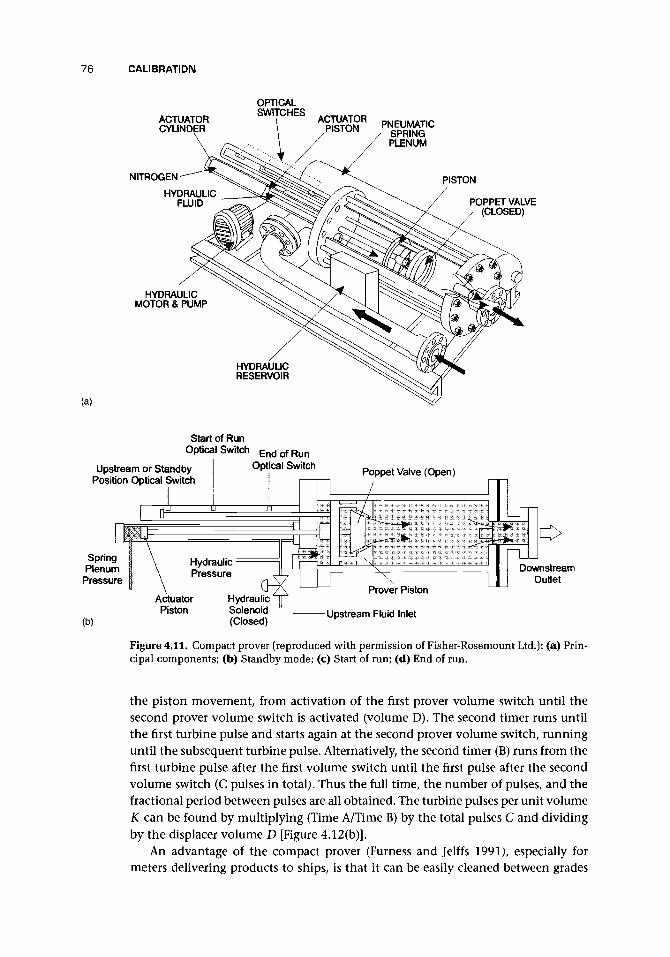
76 CALIBRATION
ACTUATORCYLINDER
NITROGEN
HYDRAULICFLUID
HYDRAULICMOTOR & PUMP
OPTICALSWITCHES ACTUATOR
PISTON PNEUMATICSPRINGPLENUM
PISTON/
POPPET VALVE(CLOSED)
(a)
HYDRAULICRESERVOIR
Start of RunOptical Switch E n d o f R u n
Upstream or StandbyPosition Optical Switch
Optical Switch Poppet Valve (Open)
SpringPlenum
Pressure
(b)
DownstreamOutlet
ActuatorPiston
HydraulicSolenoid(Closed)
Prover Piston
- Upstream Fluid Inlet
Figure 4.11. Compact prover (reproduced with permission of Fisher-Rosemount Ltd.): (a) Prin-cipal components; (b) Standby mode; (c) Start of run; (d) End of run.
the piston movement, from activation of the first prover volume switch until thesecond prover volume switch is activated (volume D). The second timer runs untilthe first turbine pulse and starts again at the second prover volume switch, runninguntil the subsequent turbine pulse. Alternatively, the second timer (B) runs from thefirst turbine pulse after the first volume switch until the first pulse after the secondvolume switch (C pulses in total). Thus the full time, the number of pulses, and thefractional period between pulses are all obtained. The turbine pulses per unit volumeK can be found by multiplying (Time A/Time B) by the total pulses C and dividingby the displacer volume D [Figure 4.12(b)].
An advantage of the compact prover (Furness and Jelffs 1991), especially formeters delivering products to ships, is that it can be easily cleaned between grades

4 .4 GAS CALIBRATION FACILITIES 77
SpringPlenum
Pressure
(c)
Start of RunOptical Switch End of Run
Optical SwitchPoppet Valve (Closed)
ActuatorPiston
HydraulicSolenoid(Open)
Upstream Fluid Inlet
End of RunOptical Switch
Fail Safe Stop\
Poppet Valve (Open)\
nSpringPlenum
Pressure
HydraulicSolenoid(Closed)
(d)
Figure 4.11. (continued).
and so eliminate contamination. It can also be skid mounted. Wherever possible,comparisons between ship and meter quantities should be monitored continuouslyto provide warning of meter factor drift (cf. Hannisdal 1991 on alternative meteringconcepts to reduce space and weight).
4.4 GAS CALIBRATION FACILITIES
4.4 .1 VOLUMETRIC MEASUREMENT
The bell prover uses a standing start and stop. Figure 4.13 shows the main features.An inverted vessel - the bell - is held by a cable and counterweight so that it dipsinto a sealing fluid. This is usually water or a light oil. The flowmeter to be calibratedis connected into a pipe that allows the gas in the gas cavity under the bell to flowout. The bell is allowed to sink into the liquid so that the gas is expelled fromthe cavity through the outlet pipe and so through the flowmeter under test. It istherefore possible to take the height of the vessel at start and end and to deducethe volume of gas that has passed. For high accuracy, various other factors needto be taken into account. The volume of gas in the vessel will be affected by thepressure and temperature within the vessel. To a lesser extent, it will be affected

78 CALIBRATION
1 1 1 1 1 1 1 11
SECONDTIMER
1ALTERNATIVE
FIRST TIMER
|
1
1SECOND
(A)
TIMER (B)
i i 1 i 111IISECOND .TIMERJ
1
1ST PROVER DETECTORVOLUME SWITCH
(a)
2ND PROVER DETECTORVOLUME SWITCH
FIRST DETECTOR SECOND DETECTOR
QL
-CALIBRATED VOLUME
FIRSTDETECTOR SWITCH
FINALDETECTOR SWITCH
MEASUREMENTPISTON
VOLUME'D'
TIMEW/VWV —
PROVEN VOLUME
ELAPSED TIME TOCOLLECT WHOLE
FLOWMETER PULSES
(b)
TIME AD TIMEB
Figure 4.12. Interpolation of flowmeter pulses for compact prover. (a) Generalconcept and double chronometry method for pulse interpolation (after Reid andPursley 1986). (b) Double chronometry method as used by Fisher-Rosemount(reproduced with permission).

4.4 GAS CALIBRATION FACILITIES 79
COUNTERWEIGHT
GASMOTION
VALVE
Figure 4.13. Bell prover.
by change in the volume of the vessel. Thehumidity of the gas will be important if wa-ter is used instead of oil. The movementof the vessel, if continuous monitoring ofthe flow is taking place, may need to be al-lowed for. This method is particularly suit-able for small domestic gas meters and iscapable of achieving an uncertainty of aslittle as ±0.2% if particular care is taken.There are a number of elderly bell proversstill in use, but there are also some newones providing high accuracy in nationallaboratories.
A similar approach, using a large bagof known volume, accommodates larger volumes.
Bellinga and Delhez (1993, cf. Bellinga et al. 1981) of Nederlandse Gasunie,Groningen, described the conversion of a portable piston prover for liquids to usewith gases; the prover is capable of flows from 20 to 2000 m3/h. The cylinder lengthwas 12 m with a measuring section of 5.22 m, diameter of 0.584 m, and volume of1.3988 m3. They also described the traceability chain before the prover came intooperation. During the initial calibration of the piston prover, the volume was de-termined by weighing the quantity of water displaced by the piston when movingthrough the measuring section. A dynamic calibration was achieved by using a mas-ter meter. As a check, the volume displaced was obtained from measurement of thedimensions of the prover. They claimed that these different methods should agreeto within 0.03%. The pressure difference needed to drive the piston at 150 m3/h was20 mbar, but at lower flow rates the motion became unsteady and was corrected byreducing the mass of the piston and adding a dynamic damping system. Bellingaand Delhez also mentioned other small changes to valves, valve operating speed,and electronics that include pulse interpolation. The aim was for the prover to beaccepted by the Netherlands Measurement Institute as the primary standard for highpressure gas meter calibration. The meters calibrated from this prover should havean uncertainty in meter factor of as good as 0.1-0.15%. Reid and Pursley (1986)considered the use of nitrogen as a pressure-balancing gas to reduce the differentialpressure across the piston and hence to reduce the leakage and to provide stabilityof motion at low flow rates.
Reid and Pursley claimed 500:1 operation in air for pressures greater than 30 barwith agreement to 1% and repeatability of order 0.25% up to 8 bar.
Jongerius et al. (1993) described a new low flow test facility consisting of four mer-cury seal piston provers at the Nederlands Meetinstituut with an operating range of2 x 10~5-3.5 m3/h at approximately ambient conditions and operable, in principle,on any gas. The low flow facility is traceable to the primary length standard, anduncertainty is about 0.2% for the smallest prover and 0.15% for the others.
4.4.2 MASS MEASUREMENTFigure 4.14 shows the scheme for a gravimetric calibration facility. The systemshown depends on the use of critical nozzles (which will be explained in Chapter 7)
FLOWMETERUNDERTEST
-WATER ORLIGHT OIL

80 CALIBRATION
CRITICALFLOW
VENTURI
DIVERTERUNIT
GAS SUPPLYAT CONSTANTPRESSURE ANDTEMPERATURE PRESSURE
CONTROLVALVES
WEIGHBRIIDGE
Figure 4.14. Scheme for a gravimetric gas calibration facility (Pursley 1986 reproduced withpermission of NEL).
as transfer standards. The facility is used to calibrate the sonic nozzles, then tocalibrate the flowmeter under test, and, if appropriate, to recalibrate the nozzles.The problem with gravimetric measurement in gases is the low density of the gasand the consequent problems of mass measurement. In addition, the flow con-trol in the calibration facility must be such that the flow rate through the me-ter under test is the same as that into the weighing vessel. The facility at theNational Engineering Laboratory, Scotland, is used for flows of up to 5 kg/s atpressures of up to 50 bar to within an estimated uncertainty of ±0.3% (Brain1978).
4.4.3 GAS/LIQUID DISPLACEMENTThe problems of calibration of gas flow has led to the use of a device that exchangesliquid flow by volume for gas flow by volume, say, by means of a piston. The liquidis metered to a high accuracy, and the gas at controlled temperature and pressure isused to calibrate the flowmeter.
Lapszewicz (1991) described a flowmeter for gas mixtures in which liquid is dis-placed, and the time and volume between two points on a tube is measured. Avalving system allows the gas to enter and be exhausted.
4.4.4 pvT METHODProvided that the gas under calibration obeys a well-defined relationship be-tween the pressure p, the specific volume v, and the temperature T (e.g., for anideal gas),
pv = RT
where R is the gas constant, the change in quantity in a pressure vessel can bededuced from the change in pressure and temperature, and the volume or mass

4.4 GAS CALIBRATION FACILITIES 81
Pressure
Temperature
CalibratedVessel
HeatExchanger
PressureControlValve
RegulatingSonicNozzle
HeatExchanger
TestMeter
Figure 4.15. Diagram of a typical facility for the pvT calibration method (Pursley 1986 repro-duced with permission of NEL).
passing through the meter under test can be deduced. A simple facility is shown inFigure 4.15. The flow and temperature of the gas are controlled by heat exchangerand pressure regulation, and the flow rate may be stabilized by a critical nozzlefollowed by a further heat exchanger.
4.4.5 CRITICAL NOZZLESThe design and operation of these devices will be described in Chapter 7. Here wenote only that they are rather inflexible in that the flow through them is, essen-tially, defined by the inlet pressure and the area of the throat of the nozzle. Thus toaccommodate a range of flows, they need to be set up as a bank of flowmeters. Atypical bank of such flowmeters is shown in Figure 7.2. The approach will be to setthese in series with high quality master flowmeters. In order that the flow range is ascomplete as possible, the mass flows through the bank need to be in a progressionsuch as 1, 2, 4, 8, 16. This will allow flow rates of 1, 2, 3, 4, 5 , . . . , 31, by suitablecombination of the nozzles (cf. Aschenbrenner 1989 who described the calibrationof a bank of 16 nozzles). In such a system, it will, clearly, be essential to have a meansof checking the integrity of the valving system so that accidental leaks do not affectthe accuracy. With this range, it is then possible to calibrate the master meters overthe same range and to use these either on the facility, or as transfer standards (cf.Bignell 1996a on comparison techniques for small sonic nozzles).
4.4.6 SOAP FILM BURETTE METHODFigure 4.16 shows a simple arrangement of the soap film burette calibration system(Pursley 1986). This is suitable for very low flow rates. The gas enters the buretteafter leaving the flowmeter, and a soap film, created within the gas flow, is driven upthe burette by the flow of gas. The movement can be observed and timed by eye, orsensing methods, probably optical, can be used to measure its transit time. Clearlythe burette will need to be calibrated for volume. Flow range is 10~7-10~4 m3/s atconditions near to ambient (Brain 1978).

82 CALIBRATION
TIMINGDEVICE
Figure 4.16. Soap film burette (Pursley 1986 reproduced with permission ofNEL).
4.5 TRANSFER STANDARDS AND MASTER METERS
Calibrated master meters may also be used to measure the flow in a specially con-structed flow facility in which the masters are in series with the meter to be calibrated.This may be the most economical approach for many manufacturers. The cost will,of course, include the regular recalibration of the master meters. Such a facility willneed careful design to achieve:
• steady flow,• fully developed flow profile upstream of both the reference (master) meter and
the meter under calibration,• adequate range for all meters to be tested,• flexible means to accommodate flowmeters of different diameters and axial
lengths and to mount them in the line, and• high quality sensing and recording systems to provide the comparison between
the meter under calibration and the master meter.
A good transfer standard should have the following characteristics (Harrison1978b):
• highly repeatable,• stable with time,• wide flow range,• insensitive to installation,• simple and robust,• compact,

4.5 TRANSFER STANDARDS AND MASTER METERS 83
• low head loss,• suitable for a variety of fluids, and• available in a wide range of sizes.
Meters suitable for use as masters for transfer standard work are, therefore, thehigh accuracy meters, which will be described in later chapters. In particular, theseinclude positive displacement meters and turbine meters. For conducting liquids,electromagnetic meters may, now, have reached a sufficient standard to be consid-ered in some cases. Ultrasonic multibeam meters may, now, also be found to beadequate, as may Coriolis meters. In gas flows, the ultrasonic multibeam may besuitable, and the critical nozzle meters, as indicated earlier, are very appropriate de-spite their inflexible flow range. Wet gas meters, although a fairly elderly design, arestill used by some standards laboratories as transfer standards.
The problem with using one meter on its own is that the stability of its signalmay not be observable, and errors may creep in without any check. For this reason,master meters are often used in pairs, either in series, so that the consistency of theirreadings is continually checked, or in parallel when one is used most of the timeand the second is kept as a particularly high accuracy meter for occasional checks.
A development to achieve very high performance and to reduce sensitivity toinstallation is the calibration of the meter with the upstream pipework and a flowstraightener permanently in position, and the use of two of these packages in series(Figure 4.17; this arrangement was suggested by Mattingly et al. 1978, with or with-out the initial flow straightener). In this way, any deviation caused by installationor by drift of one meter will appear as a relative shift in calibration between the twometers. Such meters or meter pairs are referred to as transfer standards in that theyallow a calibration standard to be transferred (with only a small increase in uncer-tainty) from a nationally certified facility to a manufacturer's facility or a researchlaboratory facility.
The meters selected as transfer standards must be capable of retaining a highperformance with removal, transport, calibration, subsequent removal, transport,reinstallation, removal, storage, etc! Several of the main flowmeter designs will meetthis requirement, and the actual selection will depend on other factors. The lineliquid should be without gas bubbles or cavitation. The meters should be selectedfor optimum range; in some cases, overlapping ranges may be an advantage.
Apart from flow profile, the pipework for transfer standard installation wouldhave the following features:
COMPLETEPACKAGE
FLOW FLOWCONDITIONERS METERS
Figure 4.17. Transfer package allowing two meters, conditioners, and pipework to be calibratedtogether.

84 CALIBRATION
PERMISSIBLEERROR
<& p
0.5r\
-0.5•\
-2
-
c
CALIBRATION POINTS
••> 1 0 20 25 40 70 100 M ^r - | ). ^ | F L Q w
PATH
Figure 4.18. Maximum permissible errors: solid line, ISO 9951; broken line, Gasunie specifica-tion (after van der Kam and Dam 1993 with permission of Elsevier Science).
• uniquely linking meters with convenient valves to control flow path and for easeof access;
• suitable environment, meeting safety requirements;• freedom from vibration and cathodic protection; and• surrounding pipework clean, in good condition, and of the same diameter as
transfer package.
Van der Kam and Dam (1993) described the replacement of orifice meters byturbines, in export stations of Nederlandse Gasunie. Even though ISO 9951 specifies aMaximum Permissible Error (MPE) as ±1% in the upper range, van der Kam and Damreported that, in their experience, turbines can operate within an envelope of ±0.5%down to about 25% maximum flow and of ±1% in the lower range (Figure 4.18).They suggested that the four-path ultrasonic meter would probably be best of all.
Pereira and Nunes (1993) described a facility with an array of ISA 1932 nozzlesas the calibration source. The sizes were such as to allow a 50:1 turndown in air, andwhere nozzles were not needed, rubber balls were inserted in the inlets to seal themoff and prevent flow. Uncertainty was claimed to be in the range 0.5-0.8%.
4.6 IN SITU CALIBRATION
A new flowmeter should have some performance specification. The need to keepdocumentary evidence on flowmeters should be reinforced. It may start well witha manufacturer's minimal or full calibration. The flowmeter should, therefore, havea known performance under reference conditions. Let us assume that this is ±1%uncertainty with 95% confidence, a reasonable and not uncommon value. Whathappens when we install this flowmeter on site?
In many cases, there may not be an adequate upstream straight length to retainthe calibration, and this may be further degraded by misalignment, etc. Let usassume that this will cause a total uncertainty of ±2%. The meter then starts itsworking life, and we cease to have any satisfactory means of predicting the likely driftthat results. Recent experience from the water industry suggests that this may rangefrom 5% to as much as 50%. Because of this uncertainty, it is necessary to determine

4.6 IN SITU CALIBRATION 85
a documentation, maintenance, and recalibration schedule for each meter. One wayto decide the period between recalibration is by experience. If, after the first recali-bration, the shift is unacceptably large, then the next period to recalibration shouldbe half the length. If the calibration is essentially unchanged, then the period maybe increased. Descriptions such as "initial period/' "essentially unchanged/' and"unacceptably large" are rather subjective, but they may be given a value based onlost revenue against costs of maintenance and calibration. The outcome of all this isthe need to recalibrate, and one choice is in situ calibration with a likely uncertaintyof, say, ±3%, considerably poorer than originally obtained on a test stand.
In deciding between the merits of test stand and in situ calibration, for a specificcase, the reader should develop a table with pros and cons in terms of ultimateuncertainty and total costs (including removal, transport, calibration, lost revenue,and reinstallation). Other factors such as damage to the meter should also be allowedfor in the decision.
Methods of in situ calibration include
• provers (sphere, piston, and tank);• other meters (transfer standards);• pipework features (inlets and bends);• drop test;• in situ meter measurement and inspection (dry calibration);• clamp-on ultrasonic flowmeters (see Chapter 13); and• probes (see Chapter 18) and tracers.
Traceability for the provers and transfer standards will be through a calibrationfacility. For other methods, traceability will be more tenuous, and in situ verificationwill be a more appropriate term.
ProversProvers have already been covered but are mentioned here for completeness. Thesphere prover (Figure 4.10) is widely used in permanent systems with banks of tur-bine meters in the oil industry. The piston prover can be trailer mounted. Claimsof order 0.1% or better are sometimes made for these devices (cf. Eide 1991 whoclaimed ±0.03%). The volumetric tank prover (Figure 4.9) discussed earlier is reck-oned capable of the same sort of accuracy level.
Other MetersAn example of a transfer standard used in a survey of domestic water consumption inScotland (Harrison and Williamson 1985) is shown in Figure 4.19 and was capable ofcalibrating meters from 0.004 to 35.7 m3/h. This was achieved by using three meterswithin the transfer standard:
• an Avery-Hardoll PD meter in series with a Kent 50-mm Helix 3000 flowmeter -range 35.7-3.7 m3/h,
• a Kent 50-mm Master 2000 flowmeter in series with a Kent 50-mm Helix 3000flowmeter - range 10.8-0.7 m3/h, and
• two Kent 12-mm PSM meters in series - range 2.7-0.004 m3/h.

86 CALIBRATION
Inlet
Outlet
Figure 4.19. Wide flow range reference meter transfer standard (Harrison and Williamson 1985reproduced with permission of NEL).
The Borda inlet chamber allowed the flow to settle prior to the Helix meter, whichis sensitive to installation.
It is obviously necessary for provers, such as this one, to be coupled into the sitepipework in series with the meter to be tested.
Pipework Features - Inlets, Bends/ElbowsThe inlet from a large tank to a pipe may be used to obtain a measure of the flowrate. The pressure difference between the inside and the outside as flow goes rounda bend or elbow may be used to obtain flow rate. The accuracy of these methods willdepend on how well-formed the pipework features are. The equations and methodsare described in Chapter 8.
Drop TestIn the drop test method, the volumetric flow through the meter is compared withthe volume change due to a level change in a reservoir (Figure 4.20). To achieve this,we require the following:
a. A suitable system with the pipework leading from the reservoir so as to allowclosure of all flows except that which leads from the reservoir to the meter undertest. There must be confidence that the water leaving the reservoir all passesthrough the test meter. There must also be a valve suitable for controlling theflow through the meter.
b. Strapping tables, which give the relationship between water level and the volumeof water in the reservoir.
c. A means to obtain level of water in the reservoir.

4.6 IN SITU CALIBRATION 87
LEVELMEASURE
Figure 4.20. Diagram of a suitable system for a drop test.
METERPIT
VALVE
d. Satisfactory means of communication between the person who is taking thelevel measurements and the person who is taking the volumetric readings onthe meter. Of course, this process may be automated.
Typical uncertainty for such a test may be
Strapping tables (say 1:10,000 dimensional precision) 0.02%Level measurement (say 2 mm in 10 cm) 2.0%Timing errors for rate (say 0.2 s in 100 s) 0.2%
Within this group of errors, although the volume of the reservoir may be affected bytank supports, etc., the level is likely to be predominant. The measurement of level,often in places with poor accessibility, small changes, and surface waves, may resultin such an error, and the preceding example may be overly optimistic for some sites.Taking the root of the sum of the squares of these errors gives 2.01%, which may beoptimistic.
In Situ Measurement of Meter Dimensions (Dry Calibration)By measuring the dimensions of a differential pressure flowmeter, it may be possibleto deduce the performance. If the measurements confirm that the design meets theISO requirements, then the flow rate should be predictable with an uncertainty ofabout 1.0-2.5%.
The term dry calibration was particularly coined for the electromagnetic flowme-ter where it is possible to measure the magnetic field strength and the meter bore andso deduce the meter performance (Al-Rabeh and Baker 1986). Although the methodshave increased in sophistication, it has been found to be not a very satisfactory ap-proach except under very carefully controlled conditions. However, an uncertaintyof order 5% may be achievable. This will, of course, require checking all secondaryinstrumentation as well as measurements of the meter geometry.
The use of retrofitted ultrasonic transducers also depends on the measurement ofpipe dimensions and the positions of the transducers. There is not enough experienceon whether this may offer genuine calibration in an in situ mode.

88 CALIBRATION
Clamp-on Ultrasonic FlowmetersThe possibility of using clamp-on transit-time ultrasonic meters is being explored.Apart from the inherent uncertainties of using such meters on pipework of unknowncondition, it is also essential to avoid installations that are seriously affected byupstream pipe fittings. These meters are discussed in more detail in Chapter 13.
ProbesProbes will be covered in Chapter 18. However, the use of probes for in situ calibra-tion is common, and a few points need to be made here.
• If a single-point measurement is required, the reader is referred to Table 2.2 whereit is shown that, for a well-developed turbulent profile, if the probe is placed nearthe three-quarter radius position (0.76 x radius from the pipe axis), the velocityat that point is approximately equal to the mean velocity in the pipe. However,this is a region of strong shear and turbulence, and incorrect positioning of theprobe may result in measurement errors. If the probe is positioned on the axis ofthe pipe, the actual positioning is less critical, but the velocity at that point is notproportional to the mean velocity in the pipe as the Reynolds number changes.Allowing for a probe calibration of ±1% uncertainty, the best that is likely tobe achieved for the total flow is of order 3% and may be much poorer thanthis.
• If the velocity profile across the pipe is required, then multiple measurementswill be necessary. These can be equally spaced, but to obtain mean velocity in thepipe it may be quicker and preferable to use an integration method that selectsfewer positions, which may or may not be equally weighted (cf. ISO 1977b, 1988and also list of standards). The log linear positioning of measurements (with eachmeasurement equally weighted) follows:
Number of pointsradially
34
5
6
Position,
0.3590.3100.9580.2780.8470.2530.773
r/R
0.7300.632
0.5660.9620.5170.850
0.9360.766
0.695
0.6350.973
Salami (1971) recommended that at least six traverse points on each of six radiiwere needed to keep errors down to 0.5% for nonaxisymmetric profiles. If weassume that the profile is axisymmetric, then we may take one diameter andselect the number of points according to the time available. The specificationof the positions, the recording of the data from the probe, and the calculationof the mean flow in the pipe are often done today by a portable flow computerdesigned for the purpose. We shall also need a value of the pipe internal diameter(ID). For further information, the reader is referred to the standards. Realisticallywe are unlikely to achieve an uncertainty of better than 3%.
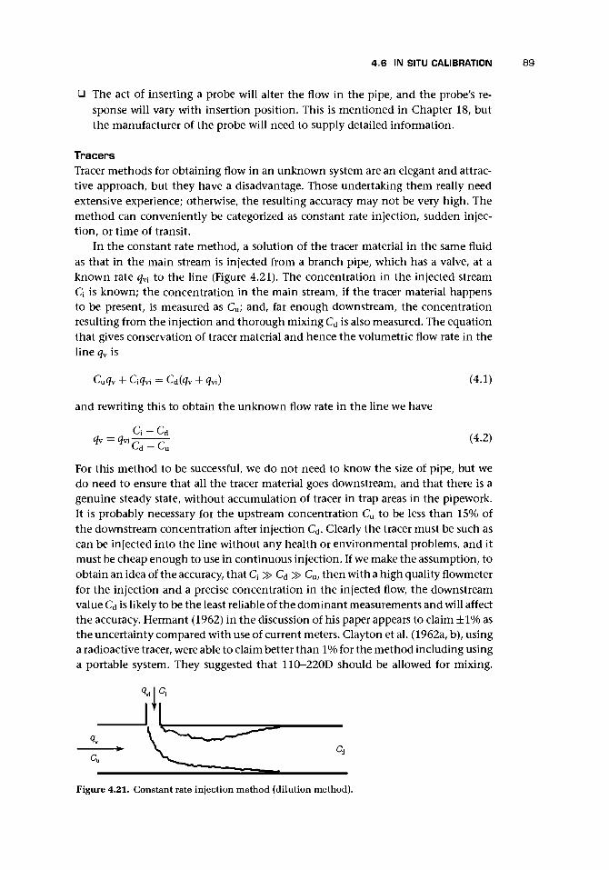
4.6 IN SITU CALIBRATION 89
• The act of inserting a probe will alter the flow in the pipe, and the probe's re-sponse will vary with insertion position. This is mentioned in Chapter 18, butthe manufacturer of the probe will need to supply detailed information.
TracersTracer methods for obtaining flow in an unknown system are an elegant and attrac-tive approach, but they have a disadvantage. Those undertaking them really needextensive experience; otherwise, the resulting accuracy may not be very high. Themethod can conveniently be categorized as constant rate injection, sudden injec-tion, or time of transit.
In the constant rate method, a solution of the tracer material in the same fluidas that in the main stream is injected from a branch pipe, which has a valve, at aknown rate qvl to the line (Figure 4.21). The concentration in the injected streamQ is known; the concentration in the main stream, if the tracer material happensto be present, is measured as Cu; and, far enough downstream, the concentrationresulting from the injection and thorough mixing Cd is also measured. The equationthat gives conservation of tracer material and hence the volumetric flow rate in theline qv is
Cuqv + Qqvi = Cd(qw + qvi) (4.1)
and rewriting this to obtain the unknown flow rate in the line we have
qv = qvi^Z^L (4.2)
For this method to be successful, we do not need to know the size of pipe, but wedo need to ensure that all the tracer material goes downstream, and that there is agenuine steady state, without accumulation of tracer in trap areas in the pipework.It is probably necessary for the upstream concentration Cu to be less than 15% ofthe downstream concentration after injection Cd. Clearly the tracer must be such ascan be injected into the line without any health or environmental problems, and itmust be cheap enough to use in continuous injection. If we make the assumption, toobtain an idea of the accuracy, that Q » Cd > Cu, then with a high quality flowmeterfor the injection and a precise concentration in the injected flow, the downstreamvalue Cd is likely to be the least reliable of the dominant measurements and will affectthe accuracy. Hermant (1962) in the discussion of his paper appears to claim ±1% asthe uncertainty compared with use of current meters. Clayton et al. (1962a, b), usinga radioactive tracer, were able to claim better than 1% for the method including usinga portable system. They suggested that 110-220D should be allowed for mixing.
Figure 4.21. Constant rate injection method (dilution method).

90 CALIBRATION
Qmean
Figure 4.22. Concentration variation downstreamwith sudden injection method (integration).
In the sudden injection method (integra-tion), one known amount of V is injectedwith a known concentration Q, and thevariation in the downstream concentrationis measured with time as in Figure 4.22.If this curve is integrated, and we assumethat the flow rate is constant during themeasurement period, we obtain the total oftracer passing, or the mean over the mea-suring period. Thus
VQ
/o(Cd - Cu) dt
VQ
(4.3)
(4.4)
where Cdmean is the mean concentration measured downstream. In addition to theconstraints for the constant rate method, the accuracy of sampling the concentra-tion is likely to be lower because instantaneous measurements will be needed andthe accuracy of the concentration sensor will introduce uncertainty. However, theamount of tracer used will be less, which may, therefore, allow a wider choice oftracer, (cf. Spragg and Seatonberry 1975).
In addition to these two methods, it may be possible to sense the passing of tracerat two points in the line, or, indeed, the variation in some naturally occurring com-ponent that might allow a correlation method to be used. It should be rememberedthat, in this case, the measure will be of velocity and not necessarily of volumetricflow (cf. Aston and Evans 1975 who estimated likely uncertainties within ±1% forsteady flows and ±2% for normally fluctuating flows).
Scott (1982) also described the Allen salt-velocity method, which measures thetime of transit between two stations between which the volume of the pipe is known.Again he mentions the need to inject the tracer explosively, in this case a minimalamount of brine, and the requirement for a sensitive detection system. The markerpoint as the brine passed each station was taken as the midpoint of the half heighttrace [Figure 4.23 (cf. Hooper 1962 and Clayton et al. 1962b who suggested uncer-tainties of order 1%)].
Various tracers have been used. For the constant rate method, sample analy-sis is likely to be the most accurate method of obtaining Cu and Cd, the values ofconcentration. In the case of sudden injection, a continuous detector will be needed.Examples follow:
Main fluid
WaterOther liquidsLiquids or gases
Gases
Tracer
BrineDyes or chemicalsTemperatureRadioactivity
Detector
Electrical conductivityColor or light sensingTemperature sensorScintillation or geiger counter
CO2, N2O, He, methane Infrared spectrometer

4.7 CALIBRATION UNCERTAINTY 91
TRACERINJECTION ELECTRODE
FLOW _JL 1_ELECTRODE
2
(a)
CONCENTRATIONOF TRACER
jA
HALF HEIGHTOF TRACES
/ \
A
MIDPOINT
NTIME
(b)TRANSIT
TIME
Figure 4.23. The Allen salt-velocity method for time of transit between two stations: (a) Pipe forwhich volume is known; (b) Marker points as the brine passes each station (after Scott 1982).
4.7 CALIBRATION UNCERTAINTY
Mattingly (1990/1) gives a very useful run down of calibration uncertainty. Beforethe facility is built, the uncertainty can be estimated. For a static gravimetric liquidfacility,
Pt(4.5)
where qy is the volumetric flow rate, Mn is the net mass of liquid collected, p is theliquid density, and t is the collection time. The uncertainties (cf. Equation 1.A.7 foralternative symbols) can be combined as
1/2
orAMn + Ap
P+ At
t
(4.6)
(4.7)
By inserting percentages of reading, an initial estimate can be obtained. Thispresupposes that Equation (4.5) is correct. However, other factors are likely to be in-volved. At the National Institute of Standards and Technology (NIST), Gaithersburg,Maryland, for liquid flow, the three values to 3 standard deviations were
— = 0.02% — = 0.01%P tMn
and combine to ±0.03% for Equation (4.6) and ±0.05% for Equation (4.7). For gas,the volume was 0.04%, density pressure effects were 0.13%, temperature effects were0.05%, and collection time for the device was 0.01% and for switching was 0.02%,giving totals of ±0.15% and ±0.25%, respectively. The next stage is to obtain data

92 CALIBRATION
from the facility, and the third stage is to obtain systematic errors from round-robin tests. These round-robin tests are known as Measurement Assurance Programs(MAPs). The systematic error is either root-sum-squared with the random error or,preferably, obtained by straight addition.
A satisfactory transfer standard is formed by using two meters, often turbines,with a flow conditioner placed between them in a tandem configuration (Figure4.17), as already mentioned for laboratory flow facilities. Adequacy of the data is es-tablished by specifying the number of repeat calibrations done for each flow rate andmeter configuration. These will ensure statistical significance. The Youden (1959)procedure is recommended (Chapter 1).
4.8 TRACEABILITY AND ACCURACY OF CALIBRATION FACILITIES
For a calibration to be acceptable, the ultimate source of the measurement mustbe known, and the calibration must be traceable to that standard, as in Figure 4.4.Laboratories holding national standards exist in several countries (Benard 1988), andthe address of the nearest should be available from national government informationor from laboratories such as:
Country LaboratoryUnited Kingdom National Engineering Laboratory, East Kilbride,
ScotlandUnited States of America National Institute of Standards and Technology,
Gaithersburg, MD
National standards should themselves be traceable back to more fundamentalmeasures of mass, time, and length. As a result of this, a traceability chain is formed.Each link is formed from a facility, or a flowmeter calibrated on a facility or againsta flowmeter of lower uncertainty. The chain needs to be rechecked with sufficientfrequency to ensure continuing confidence.
It should also be clear that, if a transfer standard with an uncertainty of, say,±0.25% is used to calibrate a flowmeter, the uncertainty in the flow rate measure-ment made by that flowmeter will be greater than ±0.25% due to additional randomerrors in the flowmeter.
Harrison (1978b) clarified the meaning of traceability with the following threepoints:
a. Each standard used for calibration purposes has itself been calibrated against astandard of higher quality up to the level at which the higher-quality instrumentis the accepted national standard. This is usually a unique item held in a nationalstandards laboratory, but it could, in some cases, be a local standard of equivalentquality built and operated to a national specification and confirmed as operatingto that specification.
b. The frequency of such calibration, which is dependent on the type, quality,stability, use, and environment of the lower-quality standard, is sufficient to

4.9 CHAPTER CONCLUSIONS 93
establish reasonable confidence that its value will not move outside the limitsof its specification between successive calibrations.
c. The calibration of any instrument against a standard is valid in exact terms onlyat the time of calibration and its performance thereafter must be inferred froma knowledge of the factors mentioned in b.
The standards for mass and time are national, derived from equivalent interna-tional standards. The international one for mass is in Paris and for time is based ona fundamental frequency, which is in turn broadcast nationally.
Thus calibration uncertainties achievable at present appear to be: for liquidsabout 0.1% and for gases 0.2-0.3% or possibly better. When total mass or volume,rather than flow rate, is required, these values may be improved. On the other hand,in situ calibration is likely to be at best 2% and often 5% or lower and should be seenas a last resort in most cases. The exception is where a meter installation is equippedwith off-takes so that a high quality transfer standard prover or meter can be coupledin series and will result in an accuracy approaching that of a dedicated facility (cf.Johnson et al. 1989 for further useful discussion of component uncertainties for agas facility).
4.9 CHAPTER CONCLUSIONS
For most readers, the essential value of this chapter will be knowledge of calibrationmethods and accuracy levels, as well as signposts pointing to where to obtain furtherdetailed information.
For those in the business of designing, installing, and commissioning flow cali-bration facilities, there are some fundamental questions to be addressed, not all ofwhich may, yet, be answerable. This chapter has attempted to flag some of thesequestions and to point to relevant literature. Some of these questions concern:
• limits of accuracy for a meter in a turbulent flow;• limits of accuracy for a test stand;• the nature of flow diversion and its repeatability;• the design of provers and the interpolation of pulse trains;• ultimate in situ accuracy including
• more user-friendly tracer methods,• more experience with retrofitted ultrasonic meters,• improved confidence in clamp-on ultrasonic meters,• improved probe measurements;
• theoretical optimum accuracy as traced from national standards and round-robinmeter exchange.
Because, therefore, existing methods may not meet all needs (Paton 1988), newdevelopments continue to appear. One relatively recent development, which is nowa standard instrument, is the piston prover. Another development that appeared afew years ago is the gyroscopic load cell, which has been applied to the weighing of
94 CALIBRATION
collection tanks in some calibration laboratories (cf. Bigneirs 1996b proposal for apositive displacement gas flow standard).
For low gas flows (0.05-5 ml/s), Robinson et al. (1986) suggested
• laminar flowmeters,• bubble flow calibration (see Section 4.4.6), and• critical flow venturi nozzle
and achieved agreement of within 1% between laminar and bubble methods. How-ever, the bubble method, too, has its potential errors due to detergent build-up.
Finally, we may question whether there are other factors resulting from environ-ment, impurities, or other components in the fluid that may affect the calibrationof certain flowmeter types or the behavior of the test stand.

CHAPTER 5
Orifice Plate Meters
5.1 INTRODUCTION
The orifice plate flowmeter, the most common of the differential pressure (DP)flowmeter family, is also the most common industrial flowmeter. It is apparentlysimple to construct, being made of a metal plate with an orifice that is inserted be-tween flanges with pressure tappings formed in the wall of the pipe. It has a greatweight of experience to confirm its operation. However, it is far more difficult to con-struct than appears at first sight, and the flow through the instrument is complex.
Some key features of the geometry of the orifice and of the flow through itare shown in Figure 5.1. The behavior of the orifice plate may be predicted, butthe predictions derive from experimental observation and data. The inlet flow willusually be turbulent and will approach the orifice plate where an upstream pressuretapping (one diameter before the orifice plate) will measure the pressure at the wall,that is in this case the static pressure. (Flange and corner tappings will be discussedlater). The pressure across the pipe will have a constant time-mean value because theonly velocity across the pipe is due to turbulent eddies. The flow close to the orificeplate will converge toward the orifice hole, possibly causing a recirculation vortexaround the outside corner of the wall and orifice plate. The inward momentum of theflow at the orifice hole will continue downstream of the hole, so that the submergedjet coming out of the hole will reduce to a smaller cross-section than the hole, whichis known as the vena contracta, the narrowest point of the submerged jet. Outsidethis submerged jet is another larger recirculation zone, and the downstream pressuretapping (the one after the orifice) set in the wall or in the corner by the orifice platesenses the pressure in the vena contracta across this recirculation zone. Downstreamof this point, diffusion takes place with considerable total pressure loss.
The data on which the orifice predictions are based may be presented in threeways (cf. Miller 1996):
1. The most accurate method is to use a discharge coefficient-Reynolds numbercurve for the required geometry, which includes all dimensional effects and otherinfluences.
2. To reduce the number of curves, a datum curve is used in conjunction with cor-rection factor curves. This was essentially the procedure adopted for the BritishStandard 1042: Part 1: 1964.
3. For convenience with the advent of modern flow computers, the data are reducedto a best fit equation. This is essentially the procedure with the most recent
95

96 ORIFICE PLATE METERS
Pressuretapping
Pressuretapping
Inletprofile
Recirculation Recirculation Poordiffusion
Plate
Poorpressurerecovery
Figure 5.1. Diagram to show geometry and flow patterns in the orifice plate flowmeter.
versions of the International Standard, and its form will be dealt with in thefollowing pages.
The most common orifice plate is a metal disk spanning the pipe with a preciselymachined hole in the center of the plate; it is usually mounted between flanges onthe abutting pipes, with pressure tappings fitted in precisely defined positions and toprecise finishes. The differential pressure is measured by manometer, Bourdon tube,or a pressure transducer, and the flow is deduced from the equations and probablycomputed using a flow computer.
The importance of the orifice is its simplicity and predictability, but to achievehigh accuracy it is essential that the detailed design of the meter is the same as thatfrom which the original data were obtained, and that the flow profile entering themeter is also the same. To ensure that the details are correct, the national and inter-national standards lay down the precise requirements for constructing, installing,and operating the orifice meter. It must be stressed that departing from the standardrequirements removes the predictability and prevents the standard from being usedto obtain the flow prediction.
In this chapter, I have sought to avoid duplicating the standards or the verythorough presentation of Miller (1996) and instead have attempted to present recentpublished information on the performance of the meter. It is, therefore, essentialthat the reader have a copy of the relevant standards from which to work and, inparticular, ISO 5167-1 (BS EN ISO 5167-1). The reader is also strongly advised to seekout a copy of Miller (1996). Access to Bean (1971), Spink (1978), Danen (1985), andSpitzer (1991) may also be useful because all have extremely valuable information
5.2 ESSENTIAL BACKGROUND EQUATIONS 97
for those concerned with the design, installation, and maintenance of orifice platemeters.
5.2 ESSENTIAL BACKGROUND EQUATIONS
Mass Flow Rate EquationThe mass flow rate is related to the differential pressure by the equation (c.f. Equa-tion 2.11 for flow without loss)
qm = f (5.1)
where C is the coefficient of discharge, E is the velocity of approach factor(1 - P4)~1/2 where p is the diameter ratio d/D of orifice diameter to pipe internaldiameter, e is the expansibility (or expansion) factor, Ap is the differential pressure,and pi is the density at the upstream pressure tapping cross-section. The value ofthe volumetric flow can be obtained from this using the relationship:
<7v = qm/p (5.2)
where p is the density of the fluid at the appropriate conditions of pressure andtemperature.
Coefficient of DischargeA simple expression for the discharge coefficient is
C = Coo + & ( 5 > 3 )
where C^ is the coefficient for infinite Reynolds number, CRe is a constant for a par-ticular installation, Re is the Reynolds number based on the pipe internal diameter,and n is the index to which this is raised. The relative simplicity of Equation 5.3is not matched by the most commonly used expressions for C, C^ or CRe either intheir complexity or variety.
The development of the equation commonly referred to as the API or AGA equa-tion can be found by referring to Bean (1971) and Spitzer (1991). Reader-Harris andSattary (1990, cf. Reader-Harris 1989) reported that a joint meeting of EuropeanCommunity and American Petroleum Institute (API) flow measurement experts inNew Orleans in November 1988 unanimously accepted a new equation. API 2530was revised to include the Reader-Harris/Gallagher equation. This allowed for anadditional term for small pipes. Additional data have now allowed an adjustmentto the equation for small orifice diameters. This was reported by Reader-Harris et al.(1995).
The previous coefficient of discharge adopted by the ISO and British StandardsInstitution was given by an equation due to Stolz (1978, 1988). This equation wasretained in the standard until 1998. For details of the thorough work that has takenplace in the last 10 years or so, the reader is referred to Reader-Harris et al. (1995)and Spencer (1993) (cf. Fling and Whetstone 1985).

98 ORIFICE PLATE METERS
The result is that current American practice appears to be to use API Chap-ter 14 Section 3 (14.3) and a new expression for the discharge coefficient C hasbeen adopted by ISO, the Reader-Harris/Gallagher equation. However, the reader isadvised to refer to the document most appropriate to the application.
The form of these new equations is
C = Coo + jT-fi + Craps + Csmall orifice (5.4)
where all coefficients are functions of p. Craps includes values of L\ = l\/D and l\is the distance of the upstream tapping from the upstream face of the plate, andL'2 = lf
2/D and V2 is the distance of the downstream tapping from the downstreamface of the plate. The prime signifies that the measurement is from the downstreamand not the upstream face of the plate. CRe reflects the slope of the characteristic dueto change of Re.
I have decided to include the provisional form of the equation in Appendix 5.A.However, it is essential that the reader refers to the standard document to checkthe latest version adopted in the United States, United Kingdom, or elsewhere andto obtain all the conditions necessary for its valid use. These include ranges forparameters, detailed design, pipe smoothness, etc.
The data for the new equation appear to have been obtained for orifice plates withdiameter ratios 0.1-0.75, throat Reynolds numbers from 1700 to 5 x 10⁷, and pipediameters from 50 to 250 mm. Data points for orifice diameters less than 12.5 mmwere very scattered and were not included.
The uncertainty is in the range 0.5-0.75% for D > 71.12 mm, and the precisevalue depends on p. For small orifices, an additional uncertainty is combined arith-metically and can be of order 0.4% for D = 25.4 mm (1 in.).
Miller (1996) gave the proposed Stolz II and NEL/TC 28 equations and tabulatedthe values for these compared with ISO and ANSI/API. Perusal of the variation acrossall equations is quite instructive. A difference between the new equations of at least0.15% is quite common, with differences occasionally as high as 1% for Re = 5,000.Comparison of both old and both new gives a spread of discharge coefficients ofless than 0.1% to nearly 2%. The best agreement appears to be for p = 0.5 andRe > 10,000, where variation across all four equations is less than 0.1% to about0.5%. One benefit, therefore, of the extensive work on refining equations has beento increase our confidence in existing values of the discharge coefficient and inindicating where the main divergences from these occur. Spitzer, also, makes thepoint that the actual maximum variation in discharge coefficient obtained from themain equations for a range of Reynolds numbers from 20,000 to 2,000,000 is only oforder 0.12%. For a p = 0.5, Re = 106, and corner tappings, I estimate that the value ofC for the latest version of ISO is about 0.13% greater than for Stolz, which generallyconfirms Spitzer's comments.
Expansibility FactorThe expansibility (expansion) factor provides an adjustment factor to allow differen-tial pressure devices to be calibrated on water, an essentially incompressible fluid forthese purposes, for use on compressible gas. It, essentially, provides an adjustmentfactor to the coefficient of discharge that allows for the compressibility of the gas.

5.2 ESSENTIAL BACKGROUND EQUATIONS 99
Reader-Harris (1998) provides a review of the past development of this factor andthe current recommended equation for it. It is found to be virtually independent ofReynolds number. For many years, it was given by an equation of the form:
el = l-(a€+b€p4)^- (5.5)
where a€ and b€ are constant coefficients, K is the isentropic exponent, which foran ideal gas is equal to y, the ratio of specific heats, and if K is not known yshould be used, pi is the pressure at the upstream tapping. However, according toKinghorn (1986) the coefficients in common use in Equation (5.5) were probably inerror.
In the most recent version of the standard, a new equation for ex is given butmay be due for a further update. It is of the form
(5.6)
provided that pi/pi > 0.75. c€ is another constant coefficient. The final bracket maybe approximated by Ap/icpi if P2/P1 is very close to unity, but the work of Reader-Harris (1998) suggests that the expression in the final bracket is preferable. He gavethe following equation, following careful analysis of the data, which may now be inthe latest ISO standard:
€i = l - (0.351 + 0.2S6p4 + 0.93£8)| 1 - (^) \ (5.7)
He gave a relative uncertainty for e\ of 3.5Ap/Kpi %, which differs slightly in de-tail from that in ISO. He also gave a very useful theoretical derivation and obtained anequation that differs from Equation (5.7) by about the uncertainty in Equation (5.7).
Pressure LossThe expression in the ISO standard for the pressure loss across the orifice plate nowappears to be
Pressure loss. ^ j g ^ - C ^Jlp\\C2) + Cp2
Taking a typical value of C of about 0.6, this results in a pressure loss for a platewith p = 0.5 (and E = 1.033) of about 0.73Ap [cf. Urner 1997 who suggested thatthe previous ISO equation (for nozzles and orifice plates) gives anomalous results ifused outside the limits of applicability of the ISO standard].
An alternative for orifice plates allowed by a recent version of the standard is
Pressure loss « (1 - p19)Ap (5.9)
which, for the preceding case, also gives 0.73Ap.The most recent version appears to have provided a loss coefficient K given by
K = * * » » * 1OSS (5.10)^PV2

100 ORIFICE PLATE METERS
where
One of the most welcome changes in the latest version of the standard is the elimi-nation of the symbol a, the flow coefficient, which was of little value. It has beenreplaced by CE, to which it was equal, or other equivalent expression.
5.3 DESIGN DETAILS
Design details are set out fully in the ISO 5167 standard. It is important that thedetailed requirements are followed so that performance can be predicted, but alsoso that new data can be added to existing data, to increase our overall knowledge.In this book, some of the requirements will be touched on, but the standard shouldbe referred to for full details.
The design is, of necessity, an iterative procedure starting from the known re-quirements of, typically, design flow rate, pipe size, and differential pressure. Danen(1985) gives some helpful calculation flowcharts for each type of differential meter.The first educated guess will relate to the value of p. With this and the selected values,a new value of p is found via the flow rate equation. Iteration continues until a satis-factory value of p is achieved. However, it is likely that most users will have access toa computer program for this procedure (either from a manufacturer or in their ownsoftware library) that will enable the optimum size of plate to be obtained. Thesewill ensure a balance between too great a pressure drop through the plate and toosmall a differential pressure for measurement. It is often suggested (Miller 1996) thatthe pressure drop across the orifice plate should be of the order of 100 in. of water(2.5 m or 25 kPa) and that the beta ratio should be close to 0.5. In some cases, thismay not be achievable. The pressure loss can never exceed the difference betweensupply and demand pressures, and the minimum pressure should be kept above theliquid's vapor pressure to avoid cavitation. Figure 5.2, which has been suggested invarious forms by various people, illustrates the compromise decision that needs tobe made between these factors.
For wide-range metering, Miller suggests the use of two transmitters ranged for180 in. of water (4.5 m and 45 kPa) and 20 in. of water (0.5 m and 5 kPa).
a. The plate. Some details of the plate geometry are shown in Figure 5.3 for a pipe ofdiameter D and with an orifice diameter of d. The plate must be flat with parallelfaces, and concentric. Flatness is defined in the standards. The upstream face isthe most critical because this has a strong effect on the flow entering the orifice.In addition to the flatness, the plate must have a roughness of less than 10~4d.It is useful to indicate the correct flow direction on the plate in a position thatcan be seen when the plate is installed. The plate may have to be rather thick towithstand the forces due to the flow, and in this case the downstream edge ofthe orifice is beveled at an angle of 45° ± 15°, so that the final thickness of the

5.3 DESIGN DETAILS 101
actual orifice opening is between0.005D and 0.02D, and constant towithin 0.001D. All edges of the orificemust be clear of burrs, etc., and theupstream edge must be sharp, definedas of radius less than 0.0004d. If d isless than 25 mm (cf. 125 mm in theprevious version of the standard), it isnecessary to measure the radius to en-sure that this condition is met. Sun et al.(1996) gave an equation for change indischarge coefficient with edge radius
^ % = 0.85 ln(103r/d) + 1.74(5.12)
for 0.0002 < r/d < 0.0035. This appearsto give a rather larger change than mostof the data in BS 1042: Section 1.5:1997,although some data for D=150 mmlines indicate changes greater than
Re Preferredregion
Maximum due tohead loss or vapor
pressure Ap
in mwater
10 m
0.1 m
Figure 5.2. Compromise decision for sizing an orificeplate for water with D and D/2 tappings with a linesize of D = 50 mm.
Equation (5.12). If these are valid, then even for r/d < 0.0004, AC/C could benearly 1% high. (Sun et al. also suggested an orifice chamfered at entry andreferred to the Russian National Code RD 50-411-83.)
Two methods have been used to measure the edge radius (Hobbs andHumphreys 1990): a stylus that followed the contour and allowed magnifications
Sharp-edgeradius
< 0.0004d e<£<0.05D
• 0.005D <e<0.02D
Constant within0.001D
f f
Constant within0.001D
Figure 5.3. Plate geometry: E is thickness of the orifice plate, and e is thickness of the orifice.

102 ORIFICE PLATE METERS
Flangetappings
Pressuretappings
(b)
(c)
Carrierring withannular
slot
of up to 500, and a cast around theedge which could be sliced and polishedafter removal from the edge. Resultsto 0.005 mm are claimed (cf. Jepsonand Chamberlain 1977 who describedBritish Gas's orifice radius inspectionsystem).
b. Pressure tappings. There are three stan-dard methods of sensing the pres-sure drop across the orifice plate(Figures 5.1 and 5.4): D and D/2tappings (Figure 5.1), flange tappings(Figure 5.4), and corner tappings (Fig-ure 5.4).
Again the standards set out the pre-cision of positioning of the tappingsand the details of their manufacture (cf.Zedan and Teyssandier 1990, who con-cluded that the tolerances that ISO andANSI/API 2530 allowed for pressure taplocations were conservative).
5.4 INSTALLATION CONSTRAINTS
The upstream and downstream pipe lengthsare set out in some detail in ISO 5167-1.A sample of the information is given inTable 5.1. The values given are claimed toretain the predicted performance of the ori-fice plate, whereas the values in parenthe-ses increase the measurement uncertaintyby 0.5%. For instance, a meter with ft = 0.5mounted within 14D of a 90° bend but withmore than 7D clear pipe upstream and 3Ddownstream will have an uncertainty in thecoefficient of 0.6 + 0.5 = 1.1%.
Reader-Harris and Keegans (1986) sug-gested that 2.5D of smooth pipe upstream
of corner tappings reduced the effect of pipe roughness further upstream. Sindtet al. (1989) found up to 1% change in coefficient for p = 0.74 and Re = 7 x 10⁶
between smooth (2.8 /xm) and rough (8.9 /xm), but for p = 0.5, the change was notmeasurable.
Constraints are also placed on thermometer pockets near to the flowmeter.The validity of these values is based on many tests to obtain data. Some recent
measurements are compared later.
Figure 5.4. Layout of pressure tappings (after ISO5167-1): (a) Flange; (b) Corner — ring with annularslot; (c) Corner — individual tappings.

5.4 INSTALLATION CONSTRAINTS 103
Table 5.1. Examples of installation requirements for zero additionaluncertainty from the standard. (Bracketed values are ±0.5% additionaluncertainty.)
1 """"ii1 p1 0.21 0.31 0.41 0.5
1 0<61 0.7| 0.75
Single90° Bend
10(6)10(6}14(7)14(7)18(9)28(14)36(18)
Upstream Straight LengthsTwo 90° Bends inPerpendicularPlanes
34(17)34(17)36(18)40(20)48(24)62(31)70(35)
Reducer 2Dto D Over1.5D to 3D
5556(5)9(5)
14(7)22(11)
Gate ValveFully Open
12(6)12(6)12(6)12(6)14(7)20(10)24(12)
Downstream
4(2)5(2.5)6(3)6(3)7(3.5)7(3.5)8(4)
BendsSome tests have raised questions as to whether the required upstream straight lengthof pipe is adequate (Branch 1995). Decrease in bend angles does not necessarily re-duce the disturbing influence on the meter (Himpe et al. 1994). There does notappear to be an optimum angle between the tapping position and the plane of thebend (Branch 1995), although a considerable influence has been noted by Himpeet al. (1994). Mattingly and Yeh (1991) gave the effect of distorted profile causedby elbows upstream of orifice meters and for the same but with a tube bundlestraightener between 3.8D and 5.7D from the bend outlet. A sample of the resultsis shown in Figure 5.5. They concluded that this flow conditioner may introduceerrors. Conditioner/flowmeter combinations should preferably be calibrated as oneunit.
Fittings that Induce SwirlMattingly and Yeh (1991) also showed that, for Reynolds numbers between 104 and105 in a 50-mm water flow facility, the angle of swirl caused by the double elbowout of plane configuration decreased from about 18° to about 6° after 40D andto about 3° after 80D. They questioned the 2° swirl criterion for safe operation oforifice installations (cf. Brennan et al. 1989 and Morrison et al. 1995 whose workmay require a knowledge of the level of swirl in a particular pipe installation).
Morrison et al. (1990a) gave measurements that confirmed that larger beta ratioorifice plates are more sensitive to swirl. They noted that expansion of the orificejet (vena contracta) leaving the plate, resulting from conservation of angular mo-mentum, would be expected to have a greater effect on small beta ratios, contraryto experience. On the other hand, the results of Brennan et al. (1991) appear tobe contrary to expectation with increased beta ratios in most cases improving theperformance downstream of tees and two elbows in perpendicular planes. In addi-tion, the results show a much better performance by the straighteners than foundby Sattary (1991), which is referred to later.
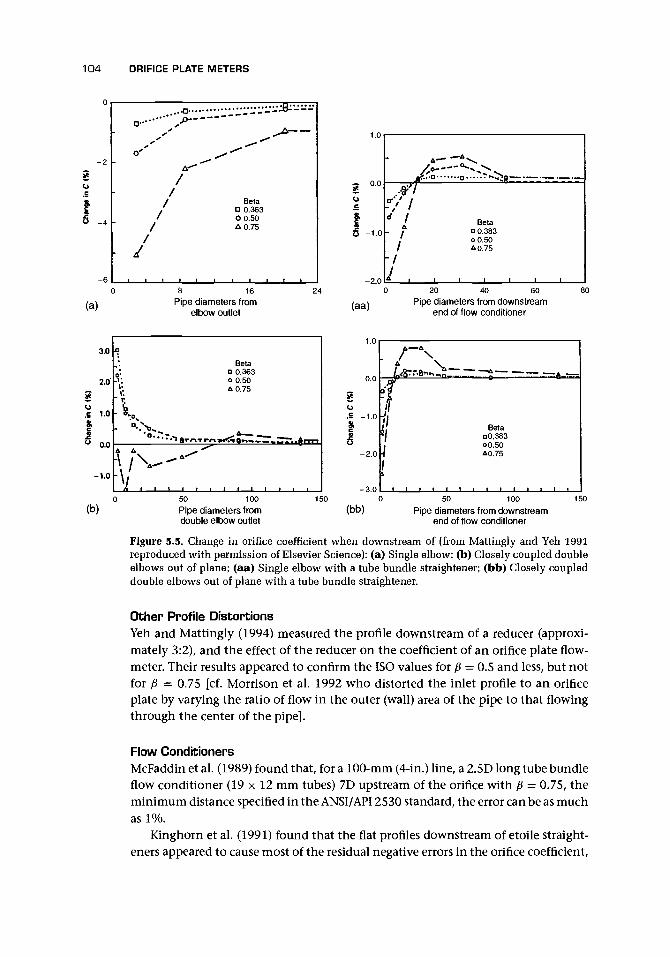
104 ORIFICE PLATE METERS
*
.E //
//
• /
i i i i i
BetaD 0.3630 0.50A 0.75
i i i i i i
(a)8 16
Pipe diameters fromelbow outlet
3.0
2.0 -'
.£ 1.0
0.0
-1.0 -
•
- V^
" V ,
BetaQ 0.3630 0.50A 0.75
(b)50 100Pipe diameters fromdouble elbow outlet
.£
O -1.0
-2.0
(aa)20 40 60
Pipe diameters from downstreamend of flow conditioner
(bb)50 100
Pipe diameters from downstreamend of flow conditioner
Figure 5.5. Change in orifice coefficient when downstream of (from Mattingly and Yeh 1991reproduced with permission of Elsevier Science): (a) Single elbow; (b) Closely coupled doubleelbows out of plane; (aa) Single elbow with a tube bundle straightener; (bb) Closely coupleddouble elbows out of plane with a tube bundle straightener.
Other Profile DistortionsYeh and Mattingly (1994) measured the profile downstream of a reducer (approxi-mately 3:2), and the effect of the reducer on the coefficient of an orifice plate flow-meter. Their results appeared to confirm the ISO values for f$ = 0.5 and less, but notfor p — 0.75 [cf. Morrison et al. 1992 who distorted the inlet profile to an orificeplate by varying the ratio of flow in the outer (wall) area of the pipe to that flowingthrough the center of the pipe].
Flow ConditionersMcFaddin et al. (1989) found that, for a 100-mm (4-in.) line, a 2.5D long tube bundleflow conditioner (19 x 12 mm tubes) 7D upstream of the orifice with fi = 0.75, theminimum distance specified in the ANSI/API 2530 standard, the error can be as muchas 1%.
Kinghorn et al. (1991) found that the flat profiles downstream of etoile straight-eners appeared to cause most of the residual negative errors in the orifice coefficient,

5.4 INSTALLATION CONSTRAINTS 105
as opposed to the positive errors due to swirling flow. To ensure an error of less than±0.5%, a straightener ID long should be placed upstream at least
• 6D for plates with a beta ratio of 0.5 and• 14D for plates with a beta ratio of 0.8.
Even with 16D separation, virtually all tests suggested some effect from the straight-ener.
Karnik et al. (1994) tested the effect of a 19-tube bundle in a 101.6-mm linefor good flow conditions and downstream of an elbow and looked at the effect onan orifice plate. Their results are very interesting in showing that even though theprofile from the tube bundle at about 20D was very close to the fully developedturbulent profile, approximating to Equation (2.4) with n = 7 A, the turbulenceintensity pattern is markedly different, suggesting that this is a factor in the re-sponse of orifice plates. They showed that the orifice coefficient downstream of theelbow and the tube bundle, compared with the correct value, was high by about0.2% between 10D and 15D and fell to about 0.1% high by about 20D. There was apoint closer to the orifice plate where the coefficients were approximately the same,but it would be unwise to rely on this for precise measurements (cf. Morrow et al.1991 who used an arrangement that allowed them to slide a tube bundle condi-tioner along the pipe between a 90° long-radius bend and an orifice plate to obtainthe variation of discharge coefficient with position for a gas flow. Overall the re-sults appeared to suggest that, if possible, the conditioner should be next to thebend.)
Sattary (1991) concluded from the EEC orifice plate program on installationeffects that the ISO 5167 and AGA Report No 3 minimum straight length specifica-tions needed to be revised. The results for conditioners 19D upstream of an orificein fully developed flows showed shifts of up to 0.33-0.5% for p = 0.57, rising toabout 0.57-0.75% for p = 0.75. For a p = 0.2, there was negligible effect from atube-bundle conditioner at 5D. The reader concerned with this topic is encouragedto refer to the original paper, which has extensive experimental data and indicationsthat there is variation between the performances of the various straighteners. Thereis some discrepancy between the various standards. For two bends in perpendicularplanes, by far the most serious disturbance, the ISO requirement for no loss in ac-curacy is that the orifice should be at least 44D downstream for a p = 0.55 and 70Dfor a p = 0.75. On the other hand, the blanket requirement for a flow straighteneris that there should be at least 20D from the fitting to the straightener and at least22D from the straightener to the meter. This is a total of at least 42D plus the lengthof the straightener, and greater than or equal to all other requirements for p up to0.75, apart from those for two or more bends in different planes. The equivalentvalues for AGA for two bends or tees not in the same plane are (Sattary 1991) forP = 0.57, 23.5D, and for p = 0.75, 35.5D, and with a short tube bundle straightenerfor the general case is 17D (straightener distance 5.5D + installation distance 11.5D).Sattary's results appeared to suggest that the values without straightener were notconclusive for ISO, but, apart from the two bends in perpendicular planes, the AGAlengths may be too short.

106 ORIFICE PLATE METERS
Orifice Plates• I Direction of flow
_ JL JL _JL _JFigure 5.6. Other orifices (reproduced with permission of Elsag Bailey-Bush Beach EngineeringDivision).
5.5 OTHER ORIFICE PLATES
Figure 5.6 gives a range of orifices that are useful for special purposes, data for someof which may be obtained from BS 1042 Section 1.2: 1989.
The quarter circle (quadrant) orifi ceplate is for low Reynolds number flows, whichresult from high viscosity liquids. The entry is more difficult to make preciselythan that of the square-edged orifice, and manufacturing tolerances are there-fore critical. An expression for the discharge coefficient in the standard has anuncertainty in the region of 2-2.5%.
The conical entrance design is for very low Reynolds number flows, which resultfrom very high viscosity liquids. The entry is again more difficult to makeprecisely than that of the square-edged orifice, and manufacturing tolerancesare therefore critical. Provided that the standard is followed, C = 0.734 withuncertainty of 2%.
Eccentric and chordal (segmental) orifices are more suitable for flows that have asecond component in them. Of these, the eccentric orifice plate is preferred,presumably on grounds of more accurate manufacture and more flexible sizingand of being defined in the standard. Thus for a liquid with solid matter, onewould choose an eccentric orifice with the hole at the bottom of the pipe,whereas for a liquid with gas entrained, an orifice at the top of the pipe wouldbe chosen. For p in the range 0.46-0.84, the standard gives the coefficient inthe range 0.597-0.629 with an uncertainty in the region of 1-2%. In caseswhere the position of the second component is not clear, it may be necessaryto go to a chordal orifice with the edge vertical to allow the second componentto pass wherever it is in the pipe.
Ball orifices (see Chapter 8).Slotted orifices (see Chapter 8).
5.6 DEFLECTION OF ORIFICE PLATE AT HIGH PRESSURE
Jepson and Chipchase (1975) provided a formula to calculate the deflection in thedownstream direction and consequent error for plates operating at high pressure.

5.B DEFLECTION OF ORIFICE PLATE AT HIGH PRESSURE 107
TEFLON SEAL (SEAL No 3 )
HETALSEAL (SEALNo 1)
DIRECTIONOF
FLOW
OIRECTIONOF
FLOW
DIRECTIONFLOW
CTRINGS
METAL SEAL (SEAL No 2 )
Figure 5.7. Differential seal ring arrangements (from Fulton et al. 1987 repro-duced with permission of the authors, the Norwegian Society of CharteredEngineers, and Christian Michelsen Research).
The original research was carried out at the British Gas Research Station inKillingworth, England. It used plates rigidly mounted between flanges and testedat differential pressures between 0 and 120 mbar.
Fulton et al. (1987) undertook further tests to determine the effect of seal ringmountings as shown in Figure 5.7 and differential pressures up to 1000 mbar. Theirresults appear to suggest that the deflection with the Teflon seal ring was generallyabout 15% greater than the values from Jepson and Chipchase's (1975) formula,whereas the results for the No. 1 metal seal were close or about 20% less and for theNo. 2 metal seal were close or about 30-40% less.
Simpson (1984) provided a useful digest of the papers by Norman et al. (1983,1984) in which this problem has been developed and experimental work undertakento validate the results. Simpson suggested that Norman et al.'s equation (essentially

108 ORIFICE PLATE METERS
that in BS 1042: Sect. 1.5: 1997)
\— Ci I
/(5.13)
where
qm = mass flow rateAp = differential pressure across the plateE* = elastic modulus of plate materialD = orifice plate support diameterh = thickness of orifice plate (=E in Figure 5.3, following ISO 5167)
could have simpler expressions for a\ and C\ than given by Norman et al. becausethe plate thickness will usually be fixed by the next most appropriate thickness ofmaterial. Simpson, therefore, gave (as in the standard)
fli =0(0.135-0.1550)d = 1.17-1.O6013
To avoid plastic deformation, the differential pressure must be below
h6(0.454-0.4340)
(5.14)
where
Meteringerror
Slope
0.2
0.1
ory = yield stress for plate material0 = orifice plate diameter ratio d/D
With Equations (5.13) and (5.14), it is possible to design for an error of, say, notmore than 0.1% for a certain working pressure and for safe operation without plastic
deformation with fault conditions of flowand differential pressure drop.
For a working differential pressure ofup to 500 mbar (and up to 1000 mbar un-der fault conditions without yielding) for0 = 0.4 with 304S.S plate material havingE* = 195.4 x 10⁹ Pa and ay = 215 x 106 Pa,Simpson obtained values of
h/U > 0.016 for required maximumerror
h/D' > 0.014 to avoid plastic deforma-tion
h must, therefore, be equal to or greaterthan 0.016D'. It should be noted that,in extreme cases of high differential pres-sure, the allowed thickness according to the
Figure 5.8. Metering error due to initial lack of plateflatness (from Simpson 1984; reproduced with per-mission of the Institute of Measurement and Control).

5.7 EFFECT OF PULSATION 109
standards may be exceeded in meeting these plate bending requirements. The stan-dard also implies that a safety factor on aY (of three) is a wise precaution.
Figure 5.8 gives curves for errors due to flatness slope against p ratio.
5.7 EFFECT OF PULSATION
In considering the installation of a flowmeter, the assumption is usually made thatthe flow is steady. In many cases, this is probably a fair assumption. However, thereare situations when it is not the case (e.g., when a reciprocating compressor, aninternal combustion engine, or some form of rotary valve is in the line). It is oftenvery difficult to decide whether the flow is indeed steady or pulsating in some way.
We might idealize the pulsating flow as consisting of a sinusoidal ripple super-imposed on a steady flow. This idealization is probably seldom valid, and little willactually be known about the amplitude, frequency, or flow profile. Mottram (1992,cf. BS 1042 Section 1.6, which uses some of his work), after the wise comment, "Ifyou can't measure it, damp it!" made some additional useful points.
• If the frequency is above about 2 Hz, differential pressure transducers will, gen-erally, be too heavily damped to pick it up. (Transducers with a response up to 2kHz or more are likely to be specified and to be more expensive.)
• The standard describes some detection techniques including the use of a thermalprobe to sense the presence of pulsation.
• Some flowmeter signals show indication of pulsation.• In some cases, the error may be deduced from the raw flowmeter signal.• Connecting leads in differential pressure meters can cause resonance and con-
fusing effects.
The orifice plate meter is affected by pulsation, and so it is necessary to reducethe pulsation and to have an idea of the error likely from any residual pulsation.
The effects of pulsation on an orifice meter are:
a. Nonlinear (square root) error. If a signal is averaged to obtain a mean flow, it isnecessary that the instantaneous flow be proportional to the signal. If this is notso, an error will be introduced.
b. Inertia error. If the fluid does not follow the changes in the flow rate instanta-neously, an error due to the inertia of the fluid will result.
c. Velocity profile effect This effect is a result of the change in profile from fullydeveloped to the unsteady flow.
d. Resonance. Resonance occurs because some component of the system is resonat-ing at the pulsation frequency.
e. Limitations in the pressure measurement device. If the pressure measurement devicedoes not respond correctly to pulsating flow, the pressure measurement may beincorrect.
Of these, the most important are (a), (d), and (e), the last two of which arerelated. The latter two are particularly possible in the connecting tubes between the

110 ORIFICE PLATE METERS
flow tube and the transducer, and because of the rate of response of the transducer.A manometer will possibly be of little value in an application with pulsation.
Thus for (a), Gajan et al. (1992) reviewed work that showed that, for quite highvalues of the ratio of rms fluctuating pressure difference to steady pressure difference,up to 0.5 at least, the main error is due to the square root effect and can be eliminatedwith a high speed response transducer. Even with a slow response transducer, theerror for the ratio, if within 0.1, may be within about 1%.
Botros et al. (1992) looked at (d) and (e) and found that the combination of linesand transmitter form a resonator that can amplify or attenuate. They recommendedthat very short lines of essentially constant diameter and a transmitter with a smallvolume and a high frequency response should be used.
Commercially available differential pressure transmitters are generally unsuit-able for dynamic measurement (Clark 1992). The dynamic response of differen-tial pressure transducer systems is significantly affected by length of transmissionline and whether the measurement medium is liquid or gas. Gas and liquid linesappear to be susceptible to oscillations, and in liquid systems there is a need forproper gas venting arrangements. Considerable care is required in order to makereliable dynamic measurements particularly when using a liquid medium (Clark1992).
The square root problem is shown by
\ f JKpdt< I- f Apdt (5.15)t Jo V t Jo
A transducer with pressure connections that is capable of responding within a timethat is short compared with the period of the fluctuation, and the signal of whichis square-rooted immediately and then averaged, will give the correct average value.This is essentially the left-hand side of the inequality (5.15). On the other hand,if the pressure is averaged and then the square root is taken, this is essentially theright-hand side of the inequality and the apparent flow rate will be high comparedto the actual flow rate. Mottram's (1981) results for pulsation error are shown inFigure 5.9(a), and they suggest that the experimental results confirm the dominanceof the square root error when compared with errors (b) and (c). However, Mainardiet al. (1977) appeared to suggest that (b) and (c) cause a change in the coefficient sothat the effect of pulsation for a fluctuating ripple of 6% of the mean flow will causean error if pulsation is measured with a high frequency response transducer of 1.5%,whereas the error is 4% for a 15% ripple. (Frequencies appeared to be up to about50 Hz.)
Williams (1970) identified the possible sources of error when manometric devicesare used to indicate mean differential pressure in a pulsating flow as
• wave action and resonance effects in the connecting leads,• volumes of ducts of varying section within the manometer and leads, and• restrictions in the leads, which cause a nonlinear relationship between flow and
pressure drop and result in nonlinear damping.
The effect of pulsation on a manometer is shown in Figure 5.9(b).

5.7 EFFECT OF PULSATION 111
LLJDCsDCLLJ
'\theoreticalsquare root
(a)
03 04 05 0-6rms PULSATION AMPLITUDE
MEAN DIFFERENTIAL PRESSURE
07 08
DC
2DCLLJDCLLJ
(b)
3 0
2 0
1 0
0
-1-0
- 2 0
o - sineA - non-sine
A
o A A) O O^ OQ
O O 6v
o
A
A
toA
ooo°
A
A
AA
A
5>AOO
A
AA A
O A
°T
ooA
A
0
° A
0 ^ A0
§ \0 A O
kjO A O
° o°OO A O^
A
A
A
A A
O A_O°_A| O—
o
O
0-1 0-2 0-3 0-4 0-5 O0-6 0-7rms PULSATION AMPLITUDE A
MEAN DIFFERENTIAL PRESSURE
Figure 5.9. Effect of pulsation on pressure measurement (from Mottram 1981;reproduced with permission of the author and of the Instrument Society ofAmerica): (a) Total error at low pulsation amplitude; (b) U-tube manometererror.
Before leaving the subject of pulsation effects, it is important to include a furthernote (cf. Section 2.6) on the Hodgson number:
(5.16)qy p
where V is the volume of pipework and other vessels between the source of thepulsation and the flowmeter position (Figure 2.5), Ap is the pressure drop over thesame distance, f is the frequency of the pulsation, qv is the volumetric flow rate,and p is the absolute line pressure. With this number, it is possible to plot curves toshow the likely error levels for various values of H. Oppenheim and Chilton (1955)

112 ORIFICE PLATE METERS
0.2 0.3 0.4Hodgson Number, H
Figure 5.10. Hodgson's number, (a) Pulsation er-ror curves for a triangular pulsation of varyingamplitude (from Oppenheim and Chilton 1955;reproduced with permission of ASME). (b) Com-parison between Hodgson's number and experi-mental results (from Mottram 1989; reproducedwith permission of Elsevier Science).
10.0
g 8°H
Uj
6.0 -
4.0 -
2.0 -
Experimental results
- O Sinusoidal
• Non-_ sinusoidal
•D Q
•
- D <2r#-HI
|
\a ]
o
°a
Frequency r«
V IV - O.E
i\ Theoretical curve, equation (5.20)\
a \
° V• ^•OB°ao^5 ^—.
jnge 5-50 Hz>
(b)0.01 0.1 1.0 10.0
have given plots of error levels for various types of flow. In Figure 5.10(a), one suchset of curves is shown.
Mottram (1989) suggested that an expression for the total error in the indicatedflow rate of a differential pressure flowmeter is
which for small amplitude ratios can be written as
Vvms/V = V2
(5.17)
(5.18)
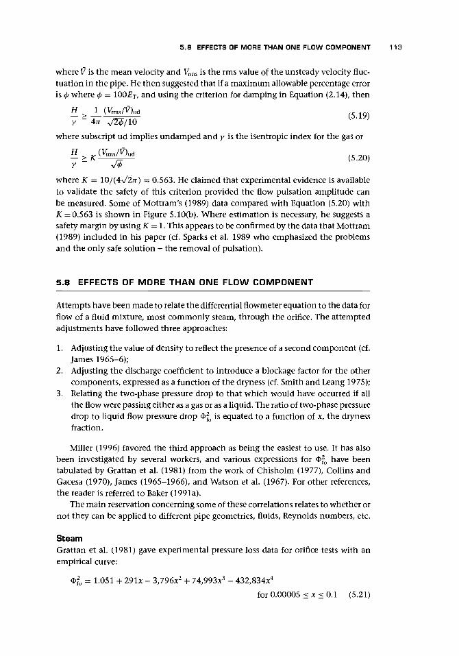
5.8 EFFECTS OF MORE THAN ONE FLOW COMPONENT 113
where V is the mean velocity and Vrms is the rms value of the unsteady velocity fluc-tuation in the pipe. He then suggested that if a maximum allowable percentage erroris 0 where </> = 100£T, and using the criterion for damping in Equation (2.14), then
H 1 (WtQud ( , 1 9 ,
where subscript ud implies undamped and y is the isentropic index for the gas or
H ( W f o d (5<20)y ~ V0
where K = 10/(4\/27r) = 0.563. He claimed that experimental evidence is availableto validate the safety of this criterion provided the flow pulsation amplitude canbe measured. Some of Mottram's (1989) data compared with Equation (5.20) withK =0.563 is shown in Figure 5.10(b). Where estimation is necessary, he suggests asafety margin by using K = 1. This appears to be confirmed by the data that Mottram(1989) included in his paper (cf. Sparks et al. 1989 who emphasized the problemsand the only safe solution - the removal of pulsation).
5.8 EFFECTS OF MORE THAN ONE FLOW COMPONENT
Attempts have been made to relate the differential flowmeter equation to the data forflow of a fluid mixture, most commonly steam, through the orifice. The attemptedadjustments have followed three approaches:
1. Adjusting the value of density to reflect the presence of a second component (cf.James 1965-6);
2. Adjusting the discharge coefficient to introduce a blockage factor for the othercomponents, expressed as a function of the dryness (cf. Smith and Leang 1975);
3. Relating the two-phase pressure drop to that which would have occurred if allthe flow were passing either as a gas or as a liquid. The ratio of two-phase pressuredrop to liquid flow pressure drop <I>j?o is equated to a function of x, the drynessfraction.
Miller (1996) favored the third approach as being the easiest to use. It has alsobeen investigated by several workers, and various expressions for <&jo have beentabulated by Grattan et al. (1981) from the work of Chisholm (1977), Collins andGacesa (1970), James (1965-1966), and Watson et al. (1967). For other references,the reader is referred to Baker (1991a).
The main reservation concerning some of these correlations relates to whether ornot they can be applied to different pipe geometries, fluids, Reynolds numbers, etc.
SteamGrattan et al. (1981) gave experimental pressure loss data for orifice tests with anempirical curve:
<$>l = 1.051 + 291* - 3,796x2 + 74,993x3 - 432,834x4
for 0.00005 < x < 0.1 (5.21)

114 ORIFICE PLATE METERS
100
i0.0000! 0.0001 0.001
Mass dryness fraction x .0.01
Figure 5.11. Experimental pressure loss data for orifice tests (from Grattan et al. 1981; reproducedby permission of NEL).
and this is shown in Figure 5.11. The scatter is an indication of the limited value ofsuch an empirical curve and of attempts to predict flowmeter performance in two-phase flows. Rooney (1973) also obtained values for the parameter 4> o (cf. Chisholm,1967; Chisholm and Leishman, 1969; Chisholm and Watson, 1966).
Owen and Hussein (1991) pointed out that if the water content was very small,the droplets would probably have a negligible effect on the flowmeter response,and so the mass flow should be corrected to allow for the mixture density ratherthan the vapor density. For wet steam of dryness x greater than about 0.9, thiscorrection is approximately F = 1/x. Owen and Hussein compare this value withother corrections in Figure 5.12(a). Note that y is the wetness fraction. In particular,BS 3812 suggested
and the Shell Flowmeter Engineering Handbook proposed
F = 1.74-0.74* for x> 0.95
(5.22)
(5.23)
Hussein and Owen (1991) referred to two correlations: James's giving a correctionfactor of
F = Pi1/2
and Murdock's
F =1.26(1 -
(5.24)
(5.25)
Figure 5.12(b) for seven alternative correlations suggests that the data scatter aroundthose of James and Murdock. Hussein and Owen (1991) showed that pressure hadlittle effect on correction factors, and that the Shell Flowmeter Engineering Handbook'scorrelation is the best compromise for x > 95% for the orifice. They wisely advocated

5.8 EFFECTS OF MORE THAN ONE FLOW COMPONENT 115
1.20
13
I 1.05-
1.000.04
(a)
0.08 0.12Moisture content
0.16 O20
1.20
1.15
1.10
|ii 1.00
0.95
0.90
0.850.82 0.84 0.86 0.88 0.90 0.92 0.94 0.96 0.98 1.00
(b) Oryness fraction, x
Figure 5.12. Wet steam flowmeter correction factor, (a) Proposed expressionsplotted against moisture content y, where x is the dryness fraction (from Owenand Hussein 1991; reproduced with permission of Elsevier Science), (b) Com-parison between data for wet steam correction factor and proposed factors fromthe literature (from Hussein and Owen 1991; reproduced with permission ofElsevier Science).
(1) x"1
(2) Separated flow model(3) Murdock's correlation(4) James1 correlation(5) 'Shell Flowmeterlng Engineering Handbook*(6) Homogeneous flow model and x~*
(7) BS 3812:1964

116 ORIFICE PLATE METERS
GO
1
o
1 1.10 -
1.0
0.90 -
1OH
Symbol
OA•X
-
-
1
Reynolds number
= 1.5 x 105
= 8 x 104
= 4 x 104
= 1.5 x 10⁴
rv n n
1 1 1
gD
1
2D 6 " ©
x •
1 10.1 0.2 0.3 0.4 0.5
Oil fraction
0.6 0.7 0.8
Figure 5.13. Performance of orifice meter in an oil-in-water emulsion (from Paland Rhodes 1985; reproduced with permission of BHR Group).
an upstream separator and indicated that several types of upstream separators givea value of x > 95% with reasonably low pressure loss. Owen et al. (1991) providedfurther convincing experimental evidence for the benefits of fitting a separator ina steam line before an orifice plate. The separator, of course, should make moreaccurate flow measurement possible. They showed that slugs of water in a gas flow,trapped by valves and then released, can travel at 50 m/s or more and result in impactpressures at 5 bar tank pressure of, in some cases, well over 50 bar. One of the orificesthey used was made of 3-mm-thick mild steel and had deformed very substantiallyafter 20 impacts.
Wenran and Yunxian (1995) suggested a simple model for deducing flow rateand phase fraction for steam flows in orifice plates, and they claim that errors were,respectively, 9 and 6.5% for their model. The reader is referred to the original articlefor more details. Pressure noise has also been suggested as a means of obtainingmore information in steam-water flows (Shuoping et al. 1996). (cf. Fischer's 1995calculation for gas-liquid annular mist).
Oil-in-Water FlowsPal and Rhodes (1985) reported results of tests of orifice meters in horizontal oil-water mixtures. Figure 5.13 shows the effect of increasing oil content on each meter.
Pal (1993) tested orifices with a range of oil-in-water emulsions ranging from 30to 84% (inversion took place at 78% oil) and found that stable emulsions introducedcoefficient changes within about 3% using a generalized Reynolds number, whichis defined in the paper, but for unstabilized emulsions the changes were greater.
Other ApplicationsMurdock (1961) reported correlations to within ±1.5% for two-phase flow. Othersare reported by Lin (1982) and Mattar et al. (1979). Washington (1989) claimed

5.9 ACCURACY UNDER NORMAL OPERATION 117
good predictions using wet gas. Majeed and Aswad (1989) appear to have achievedagreement between measured and predicted flows based on a correlation by Ashford-Pierce when using oil field data. They included a computer listing.
5.9 ACCURACY UNDER NORMAL OPERATION
To achieve the accuracy set out in the standards, it is necessary to construct andinstall the meter to the detailed specification of the standards.
From the equation
the standard provides a formula for the total uncertainty (cf. Equations 1.A.7 and7.17 for alternative symbols) in the mass flow rate:
where a, (=CE) the flow coefficient, has now been eliminated. To obtain the overalluncertainty, the uncertainty in each term is obtained and combined according toEquation (5.26).
It is instructive to put some values into this equation. Let us set out some valuesand the likely errors in them:
ParameterD
dPC
E
€
P
Value100 mm
50 mm0.50.6051
1.032811,000 kg/m3
Uncertainty %0.2
0.1-0.5
negligible-0.1
CommentWill depend on pipe
specification.Machine to 0.002 in. or 50 /mi.Equal to d/D.From ISO formula or table
(value of Re is assumed, butiteration is normally required).
Incompressible liquid.Possible variation due to
temperature or purity.Ap 31.54 kPa 1
From these values, we obtain
qm = 9.75 kg/s (Re = 1.24 x 10⁵)
{ 1 1/2(0.5)2 + (0)2 + (0.133)2(0.2)2 + (2.133)2(0.1)2 + - ( I ) 2 + -(0.1
4 4
= 0.89%

118 ORIFICE PLATE METERS
The estimate of uncertainty for gas metering is likely to be considerably larger thanthis figure. In a paper describing the specification, installation, commissioning,and maintenance of typical orifice metering stations for the British Gas nationalhigh pressure transmission system, with flows up to 1.4 x 10⁶ std m3/h at pres-sures up to 69 bar, Jepson and Chamberlain (1977) concluded that, to achieveuncertainty of less than ±2%, a very rigorous checking procedure was neededto ensure that the complete measuring system remained in specification all thetime.
Miller (1996) provided a number of special corrections: for steam quality withgas-liquid flows, for saturated liquids with up to 10% saturated vapor, for drainand vent holes, for water vapor, and for indicated differential when the pressure-measuring device is at a different elevation to the differential pressure device andthe pressure lines are filled with fluid of a different density.
Ting and Shen (1989) commented that the majority of natural gas flow measure-ments in the United States were determined by orifice meters. They led a systematicstudy of measurement by 152.4-mm (6-in.), 101.6-mm (4-in.), and 50.8-mm (2-in.)meters in the Reynolds number range 1 million to 9 million.
Ting and Shen used Honeywell smart static and differential pressure trans-ducers, which had microprocessor-based built-in pressure and temperature com-pensation, higher span-turndown ratio, improved accuracy, and easy rangeabil-ity. Bias was quoted as better than ±0.15% for differential pressure and preci-sion as ±0.015%. A precision aneroid barometer of 0.1% full-scale uncertaintywas used for atmospheric pressure. Careful calibration of these instruments tookplace, and the paper implied careful experimentation, the only weakness be-ing that the definition of the inlet pipework was not entirely clear. Their testsshowed that the 101.6- and 50.8-mm orifice discharge coefficients agreed withthe ANSI and ISO standards within the estimated uncertainty levels of 0.35%with 95% confidence level. However, the 152.4-mm meter agreed for low andmedium beta ratio, but for a beta ratio of 0.74, ANSI and ISO gave a dischargecoefficient about 2% low. Their plots also, helpfully, show the divergence be-tween the two previous standards, which is not more than about 0.2% over therange.
5.10 INDUSTRIALLY CONSTRUCTED DESIGNS
Orifice PlatesOrifice plates can be obtained from various manufacturers machined to therequirements of ISO 5167 (BS 1042) in stainless steel 316, 321, 304, Hastelloy, tanta-lum, Inconel, and plastics such as polytetrafluoroethylene (PTFE), polyvinylchloride(PVC), and polyvinylidene fluoride (PVDF). Also available are orifices that are remov-able from the holding ring, with integral gaskets that maybe spiral wound in stainlesssteel or of PTFE or graphite filled. Size availability extends beyond the common stan-dard's range going down to a 25-mm bore or less. The orifices will then be stampedpermanently with detailed information (e.g., tag number, pipe size, rating, orifice

5.11 PRESSURE CONNECTIONS 119
diameter, material), usually on the up-stream side. (Figure 5.14). The informationwill also state which is the upstream side ofthe plate.
Orifice Plate Carrier AssembliesSome examples of orifice carrier assembliesare shown in Figure 5.15(a). The materialsof construction are generally carbon steels,but stainless steels and duplex steels can beprovided. Carriers can be split ring or onepiece integral design.
Orifice Metering Run AssembliesOrifice metering run assemblies are con-structed to the appropriate standards andmay incorporate flange tappings [Figure5.15(b)]. Although plates are relatively easyto install and remove, there are occasionswhen a plate needs to be inspected withoutdisrupting the flow or depressurizing theline. For this reason, at least one manufac-turer (Figure 5.16) has developed a systemfor removing and replacing plates withoutshutting the line down. This consists of ameans for sliding the orifice plate in andout, possibly with a rack and pinion mech-anism, and a dual chamber pressure sealing
. , . , ., , . . , Figure 5.14. To indicate the main features of indus-system while the plate is removed. , .5, ' , A . , , .iL . . fJ r trial orifice plates (reproduced with permission ofDaniel Europe Ltd.).
SizingThe plate manufacturer may offer a sizing service based on a computer program thatundertakes the iteration and optimization, an otherwise laborious procedure.
5.11 PRESSURE CONNECTIONS
Tapping OrientationThe tapping positions should be such that any unwanted component of the linefluid or any second phase in the line fluid will not enter the pressure tapping of theimpulse line or become trapped in the impulse line connections. For vertical lines,any position is satisfactory (Miller 1996). Where the line is not vertical, the followingrecommendations should be noted to reduce the chances of accidental blockage (BS1042: Part 1: 1964 and Miller 1996):
• For liquids, within an angle of 45° above or below the horizontal;

120 ORIFICE PLATE METERS
Figure 5.15. Commercial orifice plate assem-blies (reproduced with permission of ElsagBailey-Bush Beach Engineering Division): (a)Carriers; (b) Metering runs.
Z- Gaskets
Orifice Flangesto ANSI B 16.36
Gaskets
Orifice Flangesto ANSI B16.36
• For dry gases, between the horizontal and vertical upward with a sugges-tion that for clean noncondensible gases the tapping should be in a verticalposition;
• For moist gases, between an angle of 30° above the horizontal and verticallyupward; and
• For steam and other vapors, horizontal only.
These requirements are illustrated in Figure 5.17. Where a drain hole is providedthrough the orifice plate, the single tapping should be orientated so that it is between90° and 180° to the position of the drain hole.
The standard also recommends that, where there is a danger of blockage, provi-sion should be made for rodding out the tapping from outside the line.

5.11 PRESSURE CONNECTIONS 121
FRONT PARTIAL SECTIONAL ELEVATION SIDE SECTIONAL ELEVATION
Figure 5.16. Commercial system for removing and replacing plates while on line (reproducedwith permission of Daniel Europe Ltd.).
Piezometer Ring ArrangementsIn pipe lines of 150 mm (6 in.) or greater,or in lines where one hole may becomeblocked, it may be useful to use a piezome-ter ring, as shown in Figure 5.18. In the pres-ence of steam or other vapor flows wherecondensation may occur, a piezometer ringmay form an unwanted trap for condensate.The manifold cross-section should alwaysbe equal to or greater than the total areaof the individual tappings which it serves.The triple T arrangement may be preferred,and, in any case, traps for condensate andadequate bleed points should be provided.In laboratory applications, the use of trans-parent tubing is recommended.
Layout of Impulse LinesIt should be remembered that, even thoughthe simple arrangement of manometerleads, with the same fluid in each, results ina deflection, the same as that which wouldoccur for direct connection to the meter
±45° Sector
Tapping
Normalcleanliquids
Tapping
Clean noncondensiblegases
Tapping
Vapors andcondensible gases
Figure 5.17. Diagram to show positioning of the pres-sure tapping for nonvertical lines.

122 ORIFICE PLATE METERS
Pressuretappings
Pressuretappings
Figure 5.18. Diagram to show piezometer ring con-nections: (a) Conventional; (b) Triple T.
line, any variation in the connecting fluiddue to air, etc., can cause variation in den-sity and a difference in the pressure acrosseach line. The effects to be guarded againstare (BS 1042: Part 1: 1964):
• Temperature difference between thelines leading to a density difference;
• Discontinuity in the impulse line fluiddue to a second component, be thatsolid, liquid, or gas; and
• Blockage of any sort including solidifi-cation of the impulse fluid.
The impulse lines should be as short aspossible, at the same temperature (whichmay require lagging together), and at a suf-ficient gradient to allow drainage, etc., asrequired.
Miller (1996) should be consulted fordetailed guidance on impulse lines, sealantliquids, and transmitter positions. A typ-ical arrangement for steam is shown inFigure 5.19.
5.12 PRESSURE MEASUREMENT
The main methods used for pressure measurement are described in Noltingk (1988)and are manometers, mechanical devices that deflect under pressure, and electrome-chanical pressure transducers.
A MANOMETER
In a manometer, the height of a column of liquid provides a measure of the pressurein a liquid or gas.
B MECHANICAL DEVICES THAT DEFLECT UNDER PRESSURE
One such device is the Bourdon tube, which has a flattened tube wound into anarc. The tube unwinds under pressure. Another design uses diaphragm elementsmade up from pairs of corrugated disks with spacing rings welded at the centralhole. Pressure will cause the assembly to elongate, and this will in turn be usedas a method of registering the pressure change. Other devices based on expandingbellows or diaphragm elements are also used.
C ELECTROMECHANICAL PRESSURE TRANSDUCERS
This is the most important and accurate device for the future and is in a state ofcontinual development. Various methods have been used to obtain an electricalsignal from a mechanical deflection. Some of these are capacitance transducers,

5.12 PRESSURE MEASUREMENT 123
Condensate level ^
Flow
Temperature Transmitter
Mains Supply
Figure 5.19. Installation for steam (reproduced with permission of Spirax-Sarco Ltd.). [Note:Tappings are often on the same side of the pipe.]
piezoresistive strain gauges, and piezoelectric and resonant devices. In one design,pressure applied to a diaphragm causes it to deflect and to exert a force on a can-tilever beam that has a strain gauge bonded to it and that provides an electricalsignal. Smart devices can provide condition monitoring, self-diagnosis of temper-ature, memory, and reference voltages and will provide ranging and temperaturecompensation. Measurement uncertainty can be as low as, or lower than, 0.1% ofspan. Regular recalibration at 1- to 6-month intervals is recommended.

124 ORIFICE PLATE METERS
TO READOUTELECTRONICS
Figure 5.20. Typical example of the installation of a density measuring cell inan orifice metering line (courtesy of the Roxboro Group PLC).
5.13 TEMPERATURE AND DENSITY MEASUREMENT
Methods of temperature and density measurement are described by Noltingk (1988).A typical installation arrangement for a density cell in a metering line is shownin Figure 5.20. The cell is arranged to project into the line so that it is at the gastemperature, and the gas is extracted from the line, passed through the cell, andreturned to the line.
5.14 FLOW COMPUTERS
Flow computers are microcomputers programmed to obtain flow from sensors mea-suring differential pressure, pressure, temperature, density, or other parameters, andare of particular importance in the calculation of the orifice plate flows. When usedwith smart transmitters, they may offer on-line optimization of differential pressuremeasurement. They contain stored information on the conversion of frequency andanalogue signals to actual units, and they contain algorithms for interpreting den-sity, etc.
Taha (1994) described electronic circuitry to obtain mass flow from an orificeplate with differential pressure, pressure, and temperature sensing.
5.15 DETAILED STUDIES OF FLOW THROUGH THE ORIFICEPLATE, BOTH EXPERIMENTAL AND COMPUTATIONAL
An early study of flow through an orifice plate using laser doppler techniques wasreported by Bates (1981) for a BS 1042 orifice plate with fi = 0.5 in the range of

5.15 STUDIES OF FLOW THROUGH THE ORIFICE PLATE 125
Reynolds number 67,600-183,000. The shape of the profiles upstream at 0.535Dand 0.32D show no recirculation zone in the plate corner, but this may be becausethe region of any such recirculation is closer to the plate than was investigated.Downstream at 0.5D the recirculation region has a zero velocity point at about 25%radius in from the pipe wall, and this moves to about the 20% radius position at0.9D downstream.
Morrison et al. (1990b) reviewed past work on flow patterns in orifice meters,both theoretical and experimental. They used a laser doppler anemometer (LDA) toobtain detailed flows in an orifice. They also obtained (Morrison et al. 1990a) wallpressure distributions, and some of these are shown in Figure 5.21(a) for a p = 0.5 atRe = 122,800 both for conditioned flow and for three angles of swirl. Figure 5.21(a)shows the pipe wall pressure distributions with a minimum pressure at about D/2downstream of the orifice plate. Note that data were not obtained between 0.125Dupstream and 0.25D downstream of the plate. Figure 5.21(b) shows the variation ofthe velocity on the centerline of the orifice meter, the high peak value at the venacontracta, and possibly a suggestion of poor diffusion.
All conditions
xlDDiameters
fromorificeplate
1.0
0.5
(b) _2xlD
Figure 5.21. Experimental curves (after Morrison et al. 1990a, 1990b). (a) Pres-sure distributions for conditioned flow and for three angles of swirl from pipewall tappings for an orifice with p = 0.5 and Re = 122,800. (b) Center-line velocity distribution using a laser doppler anemometer for an orifice with£ = 0.5 and Re = 18,400.

126 ORIFICE PLATE METERS
0.615
0.610
C
0.605
0.600
0.595104
Reader-Harris
Computed valuesfor smooth pipe
Stolz
105 106 107 108
Re
Figure 5.22. Computed values of discharge coefficient C, for an orifice withft = 0.7, corner tappings, and smooth pipe (after Reader-Harris 1989).
Erdal and Andersson (1997) provided a brief review of some computational fluiddynamics (CFD) work. They emphasized the sensitivity to the use of a particu-lar code (cf. Spencer et al. 1995). Davis and Mattingly (1997) claimed agreementbetween computed and experimental discharge coefficients to within about 4% forp in the range 0.4-0.7 and Re between 104 and 106. Sheikholeslami et al. (1988) andBarry et al. (1992) claimed an agreement of about 2%. Patel and Sheikholeslami(1986) computed the discharge coefficient for Re = 2,500,000 with p = 0.4 towithin 1.5%.
Reader-Harris and Keegans (1986) and Reader-Harris (1989) claimed that dis-charge coefficients could be calculated to within 0.64%. Figure 5.22 shows someof Reader-Harris's computations using the K — e turbulence model with a computerpackage (QUICK). In Figure 5.22, computed results for a smooth pipe and a p = 0.7are compared with the equation in the standard at that date (Stolz) and with animproved equation (cf. Reader-Harris and Sattary 1990) from which the current ISOequation has developed. Where two symbols occur at one value of Reynolds number,the higher is for the more refined grid. Reader-Harris only considered that he hadobtained independence from grid size for Re > 3 x 10⁶. His results appear to giveencouraging agreement with the modified equation.
Spearman et al. (1991) described laser doppler velocimeter (LDV) measurementsdownstream of a Mitsubishi flow conditioner and of an orifice plate in a combinedpackage.
Erdal and Andersson (1997) indicated the problems which still exist in obtain-ing adequate modeling of the flow through an orifice plate. They commented thatthe predictions revealed the need for considerable expertise and care before results,especially for pressure drop, could be predicted with confidence.

5.17 CHAPTER CONCLUSIONS 127
5.16 APPLICATION, ADVANTAGES AND DISADVANTAGES
The standard orifice can be used with almost any single-phase Newtonian flow,whereas for high viscosity fluids, a quadrant or conical orifice may be used. Abrasivefluids are likely to change the shape of the leading edge of the plate and thereforethe calibration of the orifice meter and are not to be advised. The application of theorifice plate to two-phase flows should be attempted with great caution.
An advantage of the orifice plate flowmeter is that the experience over manyyears has been well documented and is distilled in the standards, allowing a deviceto be desiged and constructed with confidence. The uncertainty is, also, calculablefrom the standards. Thus without calibration of the instrument, it is possible to seta value against the uncertainty of the measurements. Few other meters offer thispossibility.
Its ease of installation in the line has to be balanced by the need for very carefulconstruction in order to obtain the calculable uncertainty. Some features of thedesign (e.g., the edge radius of the plate inlet for small plate diameters) are verydifficult to achieve.
Another disadvantage is the nonlinear characteristic of the meter due toEquation (5.1). This, in turn, leads to a restricted range since the differential pres-sure measurement device will need to respond to, say, 100:1 turndown for a 10:1flow turndown. With smart transducers, this is more possible than in the past. An-other problem with the nonlinear characteristic is the effect of pulsation on thereading.
The high pressure loss due to the poor pressure recovery after the plate may be adisadvantage in many applications and will certainly lead to energy losses.
The cost of installation of the orifice will not be markedly less than other full-boreflowmeters, when allowance has been made for pressure transducers, flow computer,etc. Maintenance will be aided if one of the commercial designs which allows theorifice plate to be withdrawn from the line, even under operating conditions, is used.Pressure transducers should be regularly checked. This does not ensure that the totalsystem has retained operational integrity or that the calibration is unchanged bydebris in the impact pipes or by fouling or rusting of the flow pipe causing changesin roughness and hence of the profile entering the meter. However, it allows a fullerrecord to be kept without removal for calibration and, with other operating data,may give greater confidence in the integrity of the instrument.
5.17 CHAPTER CONCLUSIONS
The orifice continues to have an important and valued place in flow measurementbecause of its longevity and its documentation in the standards and because customand practice require its use in some industries. The recent update of the standard isevidence for this.
It will, no doubt, continue to have an important niche, and manufacturers oforifice meter components will continue to provide a useful service particularly forfiscal metering of natural gas and oil products (Reader-Harris 1989).

128 ORIFICE PLATE METERS
The measurement of C, of C with upstream fittings causing distortion to the inletprofile, of C with upstream conditioners, etc., has been, and will continue to be, thesubject of experimental programs. The value of such data may possibly decrease withtime, as those seeking high accuracy look to other flow metering devices. However,the orifice will continue to be specified by industry for many applications and legalreasons. The benefit of all the work that has been done, a selection of which hasbeen referred to in this chapter, is that the ISO installation requirements have beengenerally confirmed. In addition, data on the use of a flow conditioner do not yetinstill complete confidence in the resulting orifice performance (but cf. the work byLaws and others reported in Chapter 2).
Users should also be conscious of the degrading of precision that results fromcorrosion, wear, and deposits on the plate, in the pipe, and in the pressure tappings.The effect of wear on the inlet edge of the plate may be substantial.
The computation of the flow, particularly if coupled with upstream distortion,offers a considerable challenge, and the results can be sensitive to the detailed ap-plication of computer programs. It would seem to be a prime candidate for a pertur-bation approach, where the computer program could be used to calculate changesfrom the norm rather than attempt to obtain the absolute discharge coefficient. Suchan approach might shed further light on the shape of the empirical equations andthe trends in discharge coefficient for variation in D, f$, and Re (cf. Reader-Harris1989).
APPENDIX 5.A
Orifice Discharge Coefficient
I am indebted to Dr. Michael Reader-Harris for clarifying the position with regard tothe adoption of a new form of the discharge coefficient equation by ISO. At the timethat this book is going to press, the ISO has not been finalized, and the United Stateshas not changed its version to reflect the full database used in the modification.Therefore, rather than omit the equation from the book, I have decided to includethe provisional form as set out in ISO 5167-l:Amd 1: 1998 and by Reader-Harris andSattary (1996).
The equation for C, which has come to be known as the Reader-Harris/Gallagherequation, is:
for Re > 4,000 and D > 71.12 mm (2.8 in.),
C = 0.5961 + 0.0261£2 - 0.216£8 C^ term
106\( 106
—Re
0.3 Slope term

5.A ORIFICE DISCHARGE COEFFICIENT 129
+ (0.043 + 0.080e-10Li - 0.123e>-7Li) 1\ Upstream tap term
x(l-0.11A)p4(l-p4y1 J
- 0.031(M^ - 0.8M£A)p13 Downstream tap term
Where D < 71.12 mm (2.8 in.), the following term should be added:
+ 0.011(0.75 - p)(2.8 - D/25.4) (D: mm) (5.A.1)
where Re is based on the pipe diameter D,
. _ , ' 19,0000 >08
where L\ = h/D and h is the distance of the upstream tapping from the upstreamface of the plate, and L2 = V2/D and V2 is the distance of the downstream tappingfrom the downstream face of the plate. The' signifies that the measurement is fromthe downstream and not the upstream face of the plate.
The terms in A are only significant for small throat Reynolds number. M2 is, infact, the distance between the downstream tapping and the downstream face of theplate divided by the dam height.
For the purposes of Equation (5.A.I) the values of the upstream and downstreamlengths are:
D and D/2 1 0.47Flange 25.4/D 25.4/D [D: mm)Corner 0 0
The uncertainty associated with Equation (5.A.1) is
(0.7 - p)% for 0.1 < p < 0.20.5% for 0.2 < p < 0.6(1.6670 - 0.5)% for 0.6 < P < 0.75
and for D < 71.12 mm (2.8 in.), the following should be added arithmetically:
+ 0.9(0.75 - P)(2.S - D/25.4) (D: mm)

CHAPTER 6
Venturi Meter and Standard Nozzles
6.1 INTRODUCTION
In this chapter, we are concerned with devices defined in international standarddocuments. Among these, the venturi meter is one of the oldest industrial methodsof measuring flow, although other methods may be more common. Chapter 8 dealswith other devices such as variable area meters, target meters, averaging pitot tubes,Dall meters, and other venturi, nozzle, and orifice-like devices.
As in the case of the orifice plate, the reader should have access to a copy of thelatest version of the ISO standard (5167-1). I have refrained from repeating infor-mation that should be obtained from the standard, and include only the minimuminformation to provide an understanding of the discharge coefficients, the likelyuncertainty of the various devices, and the type of material from which they maybe constructed. However, although the amount of material published recently is notgreat, there is a growing interest in the use of some of these devices for difficultmetering tasks and a reevaluation of their behavior, which may well lead to severalreports in the next few years.
Spink (1978) suggested that a standard orifice should be used unless:
• The velocity is such as to require the value of f$ to exceed 0.75: if higher dif-ferential pressure or larger pipe is not possible, he suggested considering a flownozzle;
• The fluid contains a second phase of some sort - particulate, bubble, or droplet -in suspension: either a venturi or a flow nozzle with vertically downward flow,an eccentric or segmental orifice, or a different type of device such as a targetmeter or electromagnetic flowmeter should be considered;
• The fluid is very viscous or results in low Reynolds number flows: the metersalready mentioned may be suitable, or a quadrant or semicircular orifice may beworth considering;
• The flow is very low and the fluid very clean: an integral orifice or a small cali-brated meter run may be appropriate;
• Pumping costs are a major consideration: in which case go to a lower loss device.
If a liquid or a gas flows down a pipe of decreasing cross-section, the velocity(provided, in the case of a gas, that it is below the speed of sound) increases as thearea decreases, and the pressure also decreases with the increase in velocity. Thisbehavior allows the measurement of the change in pressure as a means of obtaining
130

6.2 ESSENTIAL BACKGROUND EQUATIONS 131
Upstreamtapping
Throattapping
Diffuserangle
Connectingplanes
Figure 6.1. Classical venturi meter (after ISO 5167-1 1997).
Conicaldivergent
Outletplane
the flow rate in the duct. If the duct has a smoothly varying cross-section and slowlychanging area, the pressure change for a particular flow rate can be predicted fromEquation (2.11). This is particularly so for the case of the venturi and the inlet to thestandard nozzles, and in contrast to the standard orifice plate, the flow rate can bepredicted to within about 1-1.5% as shown from experimental data.
The inlet flow will usually be turbulent and will approach the venturi (Figure 6.1)or nozzle (Figures 6.2-6A) where an upstream pressure tapping (one at entry to theflowmeter) will measure the static pressure. The convergent flow at the inlet of theventuri or nozzles passes smoothly to the throat, except that it is possible that a smallrecirculation zone may exist upstream at the corner of nozzle entry. The downstreampressure tapping for the venturi is in the parallel throat section and is set in the wall.In the case of the nozzles, the downstream tapping is either in the throat or in thepipe wall. In the latter case, it senses the pressure of the jet as it leaves the outlet ofthe nozzle. Downstream of the throat in the venturi, there is a controlled diffusion,the small angle ensuring that good pressure recovery is achieved with a low totalpressure loss. The losses at the outlet of the nozzles vary according to the particulardesign.
The comparison between the flow in the venturi (Figure 6.1), a duct of (relatively)smoothly changing area, and the flow through an orifice plate (Figure 5.1) is marked.
The essential equations governing thebehavior of the venturi and the nozzleshave been given in Chapter 2 (cf. Baker1996), and many of the ideas are touchedon in Chapter 5. In this chapter, we shall,as far as possible, avoid repetition.
6.2 ESSENTIAL BACKGROUNDEQUATIONS
Truncateddivergent
design
Not truncateddesign
The equation relating mass flow to the dif-ferential pressure for venturi and nozzles, is
Inletpressure
Throatpressure
Figure 6.2. Venturi nozzle (after ISO 5167-1 1997).

132 VENTURI METER AND STANDARD NOZZLES
Pressuretappings
(carrier ring)
\Pressuretappings(corner)
Figure 6.3. ISA 1932 nozzle (after ISO 5167-1 1997).
reproduced from Chapter 5:
(5.1)
where C is the coefficient of discharge, E is the velocity of approach factor (1 -p4)~1/2
where p is the diameter ratio d/D of orifice diameter to pipe internal diameter, e is theexpansibility (or expansion) factor, Ap is the differential pressure, p\ is the density atthe upstream pressure tapping cross-section, and qv is related to qm by Equation (5.2).
The expansibility (or expansion) factor e is given in the standard for each device,venturi or nozzle, which should be consulted for details. The expressions differ fromthose in Chapter 5.
The discharge coefficients for these instruments are of the form
(6.1)
/
ii
D
i—-
iFigure 6.4. Long radius nozzle (after ISO 5167-1 1997).

6.2 ESSENTIAL BACKGROUND EQUATIONS 133
Table 6.1. Coefficient of discharge for the classical venturi
Type ofConvergent
Rough-cast(or as-cast)
Machined
Rough-weldedsheet iron
Constraints
100 mm < D < 800 mm0.3 <P < 0.752 x 10⁵ < Re < 2 x 10⁶
50mm< D < 250 mm0.4 < p < 0.752 x 10⁵ < Re < 1 x 10⁶
200 mm < D < 1200 mm0.4 < p < 0.72 x 10⁵ < Re < 1 x 10⁶
C
0.984
0.995
0.985
Uncertaintyin C (%)
0.7
1.0
1.5
For the classical venturi meter, the coefficients are given in Table 6.1. It is im-portant to note that, although the flow in the meter is a flow that approachesthe ideal and results in a coefficient within about 1% of unity and therefore veryclose to the result from Bernoulli's equation, the uncertainty is greater than for theorifice. This reflects not on the stability of the flow but on the consistency withwhich the devices can be machined and the pressure tappings formed. The expe-rience that has been amassed of the behavior of these instruments will also relateto this.
Shufang et al. (1996) reported tests outside the ISO limits with a 1,400-mm designusing a maximum flow rate of 18,000 m3/h with a system uncertainty of 0.2% andfor 1,85 x 10⁶ < Re < 5.78 x 10⁶ obtained discharge coefficients:
for machined convergent 0.983 ± 0.003for rough-welded 0.987 ± 0.006
The results for the rough-welded are essentially in line with the annex in thestandard, which suggests no change for the rough-welded but an uncertainty of±2%. However, for the machined convergent, the standard suggests a slight increasein C and uncertainty compared with the decrease reported by Shufang et al. (1996).For the rough-cast or as-cast version, the standard suggests that there appears tobe no change for higher Reynolds numbers. There are likely to be changes, mainlydecreases in C, for lower Reynolds numbers.
For the nozzles, the standard sets out the discharge coefficient formulas. Thereader is referred to ISO 5167-1 for the complete formulas, the conditional require-ments and the limits of applicability. For ft = 0.5 and Re = 106, the terms in Equa-tion (6.1) have values:
CQO Second Term
for the venturi nozzle 0.9771 0for the ISA 1932 0.9768 -0.00025for the long radius 0.9965 -0.00462

134 VENTURI METER AND STANDARD NOZZLES
The approximate uncertainty for each nozzle for a p = 0.5 is
for the venturi nozzle 1.3%for the ISA 1932 0.8%for the long radius 2.0%
Note that in all the equations, Re refers to the Reynolds number based on theupstream pipe internal diameter. However, Red based on the throat diameter is some-times used in the standards, and the reader should be aware of this.
6.3 DESIGN DETAILS
As for the orifice plate, these are set out fully in ISO 5167, which provides the detailedrequirements. The reader must refer to the standard to confirm that these are thelatest values and to obtain all other details for each of these devices.
For the Classical Venturi MeterThe main features of the venturi design are shown in Figure 6.1. In addition thestandard deals in matters such as the smoothness of the finish of the throat and theadjacent curvature. These are required to have k/d < 10~5, where k is the roughnessand d is the throat diameter. For the machined venturi, the entrance cylinder oflength not less than D and the convergent section are required to have a finish tothe same quality. The radius of curvature between the sections must be less than thefollowing values:
0.25D between entrance cylinder and convergent section,0.25d between the convergent section and the throat,0.25d between the throat and the divergent.
In each case, the standard would prefer that the radius of curvature be zero. Therequirements for the other two methods of fabrication of the venturi are also givenin the standard.
Pressure tappings are shown in Figure 6.1, and the standard requires that four (atleast) shall be provided at both the throat and the upstream positions and specifiestheir size, finish, and precise positions.
The value of the pressure loss across the venturi meter compared with the differ-ential pressure between inlet and throat can be taken to be in the range 5-20%.
For the Venturi NozzlesThe nozzle is shown in Figure 6.2 and must have a roughness less than 10~4d. It canbe made of any material provided it meets the requirements set out in the standard.Obviously the material must be stable enough to retain its shape and to resist erosionand corrosion by the fluid.
For the ISA 1932 NozzlesThe nozzle is shown in Figure 6.3 and has a roughness as for the venturi nozzle.Again, any unchanging material is acceptable.

Flanged Nozzle Assembly
6.5 INSTALLATION EFFECTS 135
Integral Weld-in Nozzle
ISA 1932 Flow NozzleTo BS1042 Section 1.1
Orifice Flangesto ANSI B16.36with Corner Taps
Long Radius Flow NozzleTo BSI042 Section 1.1
Venturi Tube
Fabricated FlangedVenturi TubeTo BS1O42 Section I . I Figure 6.5. Commercially available devices
(reproduced with permission from ElsagBailey-Bush Beach Engineering Division).
For the Long Radius NozzleThe nozzle is shown in Figure 6.4 and has the same roughness as the venturi nozzle.Again any unchanging material is acceptable.
6.4 COMMERCIALLY AVAILABLE DEVICES
The standards allow prospective users to design and make their own differentialpressure device. However, various manufacturers also produce standard equipment.Figure 6.5 shows examples of such devices.
6.5 INSTALLATION EFFECTS
Upstream FittingsEven though the values recommended by ISO 5167-1:1997 for nozzles and venturinozzles are the same as those for the orifice plate, the values for the classical venturiare generally less. For instance, for a venturi with a diameter ratio of 0.5, the ISOallowance for an upstream bend is 1.5D, and for two or more in the same plane, itis 2.5D. These spacings have raised questions, and, as a result, NEL (1997) providedguidance on installation, which suggested that the ISO may need to be revised as

136 VENTURI METER AND STANDARD NOZZLES
Table 6.2. Upstream straight lengths required for zero additional uncertainty(in diameters from the outlet of the downstream bend to the upstream pressuretapping plane) as for ISO (old) and as proposed by NEL (1997) (new)
p0.40.50.60.75
SingleBend
Old
0.51.53.04.5
90°
.5D)New
89
1016
Two 90° BendsSame PlaneOld
1.52.53.54.5
New
3101022
Two 90° BendsPerpendicularPlanesOlda New
333
17
Reducer3:1 Over3.5DOld
2.55.58.5
11.5
4:3 Over2.3DNew
4444
Note: At least four throat diameters should separate the throat tapping from downstreamfittings.a Indicates that no values are given without 0.5% additional uncertainty.
indicated in Table 6.2. The guidance notes should be consulted for spacings where0.5% additional uncertainty is relevant.
For the venturi, Ginesi (1991) suggested that the upstream lengths, to avoidcalibration change, may be about half those for the orifice, rather than a ninth assuggested by the standards. This agrees with Table 6.2 for a single bend and twobends in the same plane, but there is less agreement for the other two columns. Themost surprising values in Table 6.2 are those for two bends in different planes, towhich most instruments are very sensitive.
Himpe et al. (1994) described new results for the influence of upstream bends onthe discharge coefficient of classical venturi tubes, which suggest that the influenceof disturbances does not necessarily decrease with decreasing bend angles, and theinfluence of the angle between the plane of the pipe bend and the position of thetapping is considerable.
Al-Khazraji et al. (1978) used an eccentric orifice upstream of a venturi to assessthe error that results from the flow disturbance. The orientation relative to the singlepressure tapping had a negligible effect, but a spacing of 5D reduced the error to about1%. At 10D spacing, there was, again, negligible effect, showing the same trend asfor a single bend with fi < 0.6 in Table 6.2.
Two-Phase FlowsBaker (1991a) provides several references relating to the behavior of venturi meters inmultiphase flows. Additionally, de Leeuw (1997, cf. 1994) proposed a new correlationfor overreading in wet gas horizontal flow which appears to give results within 2%of the data. He claims that the improvement is, in part, because it allows for the gasvelocity. Taking qtp as the volumetric flow rate deduced from the differential pressurewhen liquid is present in the gas stream, qx as the liquid volumetric flow rate, andqg as the gas volumetric flow rate, the overreading ratio is given by
(6.2)

6.6 APPLICATIONS, ADVANTAGES, AND DISADVANTAGES 137
where X is the Lockhart-Martinelli parameter and
The liquid and gas densities are given by px and pg and
n = 0.606(1 - e-° 746F'g) for Frg > 1.5 (6.4)
and
n = 0Al for 0.5 < Frg < 1.5 (6.5)
where the superficial gas Froude number is given by
(6.6)
where Vsg is the superficial gas velocity, and the Lockhart-Martinelli parameter isgiven by
(6.7)
The relationship is valid for gas densities above 17 kg/m3 and up to the liquiddensity, for gas Froude numbers above 0.5, and for Xup to 0.3 (cf. Chisholm 1977).
6.6 APPLICATIONS, ADVANTAGES, AND DISADVANTAGES
Early work on the classical venturi by Herschel was aimed at use in the water indus-try, and it has continued to be used in measurement of water flows. Where energyconservation is an important consideration in large pumped flows, the low head lossof the venturi becomes attractive.
Rivetti et al. (1994) have described a quite different application of a small sizeventuri for liquid helium service, which was essentially a scaled down ISO 5167design. Differential pressure must not be so high as to cause cavitation, and pressureducts should have a diameter between 1/10 and 1/5 of the diameter of the respectiveventuri section and be four or more (an even number). Flow rates ranged from0.5-4 g/s to 12.5-100 g/s for upstream/throat diameters of 6/2.6 and 16/12 mm,respectively, and differential pressures of 34-2,190 and 33-2,140 Pa, respectively.
The classical venturi has also been used for slurry and two-phase flows for whichsome data are available. Baker (1991a) has reviewed work on this application of theventuri. There appears to be growing interest in the use of venturi meters in theseapplications, although the behavior of the flow and the appropriate models of themultiphase flow may not be straightforward. One such example is the performanceof the venturi meter in an oil-in-water emulsion in Figure 6.6 (Pal and Rhodes 1985).
The initial cost of the venturi is higher than the orifice because it is a much largerdevice to make, and precision in manufacture may not be easy. Various manufactur-ers offer ready-made designs (Figure 6.5).

138 VENTURI METER AND STANDARD NOZZLES
1-5
ficie
nt c
coet
ual
^d/a
ctPr
edic
t*
1.10
i n1 .U
0.90
Symbol
OA
DX
-
_
-
1
Reynolds number
= 1
= 8= 4= i
5xX
5
x
|
x 105
104
104
xlO4
H
i i i i i0 0.1 0.2 0.3 0.4 0.5 0.6 0.7 0.8
Oil fractionFigure 6.6. Performance of a venturi meter in an oil-in-water emulsion (Pal andRhodes 1985; reproduced with permission from BHR Group).
The nozzles tend to be more stable than the orifice for high temperatures andhigh velocities, experiencing less wear (due to the smooth inlet contour as opposed tothe sharp orifice upstream edge) and being less likely to distort. They are particularlyapplicable to steam flows, where they have been widely used.
6.7 CHAPTER CONCLUSIONS
This chapter has been, necessarily, brief because there appears to be less significantnew material in the literature to add to the advice and guidance of the standards.However, there does appear to be an increased interest by the oil and gas industry inusing venturi meters for both single and multiphase (especially wet gas) metering,and as a result some new work, which appears to be yielding some unexpected results,is taking place (Jamieson et al. 1996).
a. It should be noted that the coefficient for the ISA 1932 nozzle has been slightlyaltered in the standard.
b. Jamieson et al. (1996) observed discharge coefficients for a 150-mm (6-in.) diam-eter venturi in high pressure air (70 bar) at Re up to 8 x 10⁶ and throat velocitiesup to 125 m/s, which were several percent higher than those obtained in watercalibration. The reason appears to lie in the tapping chambers and the possibleacoustic effects there.
c. Computational fluid dynamics (CFD) work is being developed (cf. Sattary andReader-Harris 1997) for venturi and nozzles. For venturi with f$ = 0.4, 0.6, and0.75, CFD tended to underestimate relative to experimental and ISO by up toabout 1.2%. Sattary and Reader-Harris (1997) suggest that the difference is due tothe actual method of measuring static pressure compared with the CFD model.

6.7 CHAPTER CONCLUSIONS 139
They also looked at compressibility effects. There is likely to be growing interestin developing the CFD work to explore the likely ultimate precision of theseinstruments.
d. An inside-out nozzle or short venturi in the form of a bullet-shaped target metercould yield a highly predictable meter with direct electrical output via a forcesensor. This could be combined with wall differential pressure measurements toprovide a condition-monitoring function.

CHAPTER 7
Critical Flow Venturi Nozzle
7.1 INTRODUCTION
This meter uses a fascinating effect that occurs when gas flows at very high velo-city through a nozzle. As the gas is sucked through the nozzle, the velocity increasesas the cross-section of the nozzle passage decreases toward the throat. At the throat,the maximum achievable velocity is sonic - the speed of sound. Downstream of thethroat, the velocity will either fall again returning to subsonic or will rise and becomesupersonic. In normal operation of the nozzle, the supersonic region is likely to besmall and to be followed by a shock wave that stands across the divergent portion ofthe nozzle and causes the gas to drop, very suddenly, from supersonic to subsonic.The existence of a shock wave does not mean that one will hear a "supersonic bang"!Such bangs are usually caused by moving shock waves carried forward by high speedaircraft.
The fascinating effect of sonic conditions at the throat is that changes in theflow downstream of the throat have no effect on conditions upstream. The sonicor critical condition, as it is called, appears to block any information that is tryingto penetrate upstream. A simple picture of this is that the messengers carrying suchinformation travel at the speed of sound and so are unable to make any headwayover the fast flowing gas stream.
Two important effects of sonic conditions are that
i. the mass flow rate is a function of the gas properties, the upstream stagnationtemperature and pressure, and the area of the throat, provided that the nozzleis actually running at critical conditions (which can be ascertained by checkingthe downstream pressure);
ii. the nozzle acts as a flow controller, creating steady conditions upstream eventhough conditions downstream are unsteady.
Figure 2.6(a) shows a simple illustration of a convergent-divergent nozzle witha throttle valve downstream. Figure 2.6(b) shows the variation of pressure throughthe nozzle, and the critical flow conditions are those bounded by curves c and i forwhich the flow becomes sonic at the throat.
For a fuller description of the fluid flow behavior, see Baker (1996). Two essentialequations apply when the velocity at the throat is equal to the speed of sound(Mach number equals unity) and the conditions are critical. The first equation gives
140

7.2 DESIGN DETAILS OF A PRACTICAL FLOWMETER INSTALLATION 141
the pressure ratio for choked flow [Equation (2.18)]:
Po V 2 /
where p* is the pressure at the throat, p0 is the stagnation pressure, and y is the ratioof specific heats cp/cw.
The second equation gives the ideal mass flow qm for choked flow from Equation(2.18), making use of the relationships
( 7 . 2 )
where R is the universal gas constant (8.3143 kJ/kmolK), M is the molecular weight,cp and cw are the specific heats at constant pressure and constant volume, A* is thethroat cross-sectional area, and 7o is the stagnation temperature.
Thus if we can measure upstream stagnation pressure and temperature po andTo, and if we know the throat area A* and the gas properties, we appear to have amass flowmeter. The flow must be choked. Also this equation is limited to a perfectgas and assumes an idealized and one-dimensional flow.
We are interested in the use of this device for real gases. For precise work, we haveto recognize that gases are NOT perfect. We also find that boundary layer growthand curvature of the flow through the nozzle result in a flow that is not truly one-dimensional.
Thus as with many flowmeters, there is a coefficient of discharge, to be discussedlater. First, we consider a practical flowmeter installation.
7.2 DESIGN DETAILS OF A PRACTICALFLOWMETER INSTALLATION
The critical flow venturi nozzle is fully specified by the most recent version of thestandard document BS EN ISO 9300: 1995. The reader is strongly advised to obtaina copy of the standard for reference if planning to build a facility using this deviceand to view this chapter as complementary to the standard.
Figure 7.1 shows a diagram of a critical flow venturi nozzle installation. Notethat the temperature tapping can be upstream of flow conditioners because thetemperature change is likely to be negligible. However, the pressure tapping mustbe sensing a true inlet stagnation value. There may also be a downstream measureof pressure to ensure that critical conditions are maintained.

142 CRITICAL FLOW VENTURI NOZZLE
2D±0.2D
6flow
straightener
Figure 7.1. Details of venturi nozzle installation.
straightlength>5D
D±0.1 D
ithroatdia. d
CUxl
CZXI
czxr
inletmanifold
If the upstream pressure allows only limited variation, then the range of qm willbe limited, and only by using a bank of nozzles of different areas can we achieve asatisfactory calibration range (Figure 7.2). Caron (1995) mentioned a test stand thatused a bank of sonic nozzles in binary sequence. Nozzle 2 has twice the flow rate ofnozzle 1, etc.
Nozzles may have a convergent portion only; in which case there will be asubstantial pressure loss at exit, and the pressure ratio of outlet-to-inlet stagnationmust be less than 0.528 for air. On the other hand, the convergent-divergent venturinozzle in Figure 7.3 may achieve a pressure ratio (exit/inlet) for critical conditionsat the throat of pz/po — 0.9. The one shown is the toroidal throat venturi nozzle.An alternative, not favored by some, is the cylindrical throat type where a constantarea throat of one diameter in length separates inlet contraction and outlet diffuser.
The diagram in the standard provides the details of design finishes andtolerances that differ slightly from, but cover, those in Figure 7.3. It is also impor-tant to note other features of the nozzle in Figure 7.3. The inlet pipe diameter,D, must be greater than 4d, and referring to Figure 7.1 with a pipe diameterof 50 mm upstream, this would put a maximum on the throat diameter of
12.5 mm. Also the preferred distance to theupstream pressure tapping is between 0.9Dand 1.1D. Other spacings are allowed pro-vided that it can be shown that the tappinggives a correct measure of the nozzle in-let stagnation pressure. The standard allowsfor a larger space upstream with its ownrequirements.
The standard also sets out requirementson temperature measurement that coverthe position in Figure 7.1 but allow a greaterspacing if it gives, reliably, the stagnationtemperature at nozzle inlet. The standardalso warns that care needs to be taken ifthe surroundings of the installation differ intemperature by more than 5°C from the gas.
itxrzj
3XIZ=
3>C_
>o
>c=
criticalnozzles outlet
manifold
Figure 7.2. Bank of critical flowmeters.

7.3 PRACTICAL EQUATIONS 143
2.5d
Figure 7.3. Details of toroidal throat venturi nozzle.
Where there is the possibility of condensate, drain holes are allowed providedthere is no flow through them when flow measurement is taking place, and theyare spaced upstream of the pressure tapping by at least D and not in the same axialplane as the pressure tapping.
The standard requires that the nozzle be made from material capable of finishto the required smoothness, resistant to corrosion in the intended application, anddimensionally stable so that temperature corrections can be used for throat area.
7.3 PRACTICAL EQUATIONS
The practical use of critical flow venturi nozzles is set out in BS EN ISO 9300: 1995.Apart from some nomenclature differences, this section gives the method set outin the standard. Using the expression of Equation (7.2), we introduce a dischargecoefficient C to allow for the deviation from the ideal equation, and we also introducea coefficient for the gas Q, the critical flow function, obtainable from tables andformulas, and for a perfect gas written as
(7.3)
With these coefficients, we can rewrite the equation as
A*C C*po
T0(R/M)
Alternatively, the equation may be written in terms of p0 and
qm = AtC
(7.4)
(7.5)

144 CRITICAL FLOW VENTURI NOZZLE
where
and
poPo
ZQRTQ
M
(7.6)
(7.7)
In this case, we require values of C* and Zo, the compressibility factor at stagnationconditions.
The design should, preferably, ensure that the values of p and T are obtainedwhere the Mach number is small enough to assume that they are equal to p0 and To.Otherwise, the standard gives equations to obtain the corrected values.
In order to ensure that the nozzle operates critically, the standard requires thatthe actual maximum outlet pressure p2max, when compared with the ideal value p2i,for which critical conditions are achievable satisfies
- P*= 0. (7.8)
0.9
0.85
0.8
0.75
Using tables such as those in Baker (1996), it is possible to obtain values of p2i forvarious values of outlet area A2, assuming that the gas behaves sufficiently closelyto an ideal gas to use the ratio of the specific heats y. Figure 7.4 shows the values ofp2max/po for y = 1.4. The standard provides a plot for other values of the isentropicexponent.
Note that y is the ratio of specific heats for an ideal gas, and K is referred to in thestandard as the isentropic exponent and applies to real gases. I have avoided usingthe latter in this chapter. For further information, consult Bean (1971) who relatesthe value (cf. Miller 1996, Sullivan 1979) of K to y via an expression (which he doesnot derive) that recognizes that Z is constant for an ideal gas but varies for a realgas. Miller (1996) also gives plots of K. Where there is a divergence between K andy, the standard indicates which to use.
It is relatively simple to relate the area~~~~ ratio between the throat and the outlet
based on design angles of the diffuser. If thehalf-angle of the diffuser is 0, the radius oftoroid is r and the length of the diffuser is /beyond the toroid, the increase in diameteris (Figure 7.5) 2[r (1 - cos 0)+1 tan 0] so thatthe outlet diameter
0.7
0.65
d2 = d+2[r(l-cos 6>)+/tan 0]
or1.0 2.0 3.0 4.0
AJA*5.0 6.0
2r(l-cos0) 2/ tan 0 (7.9)Figure 7.4. Maximum values of back pressure fory = 1.4 to ensure critical operation based on the cri-terion in BS EN ISO 9300: 1995.
from which the expression in the standardfor A2/A* can be simply obtained.

7.4 DISCHARGE COEFFICIENT C 145
/tane- r(1 -cose)
'T
Figure 7.5. Geometrical calculation to obtain the outlet diameter from the dif-fuser geometry.
7.4 DISCHARGE COEFFICIENT C
The data on which the discharge coefficient is based include work by Smith andMatz (1962), Arnberg et al. (1973), Brain and MacDonald (1975), and Brain and Reid(1978, 1980). Figure 7.6 shows the scatter in the data. The general equation thatgives a fit to this data is
(7.10)
and the value of the constants, including the preferred ISO values, are given in Table7.1. Figure 7.6 shows that the values fall well within an uncertainty band of ±0.5%at 95% confidence level around the BS EN ISO 9300 preferred equation.
The values of b and n are affected by the nature of the boundary layer in thethroat. Transition is likely to cause a change in these parameters. Miller (1996) alsosuggested that the temperature gradient between gas and nozzle may affect b.
0.99
0 98
—— — • —
' 1
+ 0.5%
£-. a fio f a
• • * * • * \ ^
+ Arnberg et ala Smith & MatzO NBSv Brain & MacDonald• Brain & Reid
-ARNBERG ET AL
. ISO 9300
a
BRAINS REID
(1978, 1980)
(1973)"
•
•
-
105 10 6
Throat Reynolds number-Red
107
Figure 7.6. Discharge coefficient for toroidal throat venturi nozzles (after Brain and Reid 1978with permission from NEL).

146 CRITICAL FLOW VENTURI NOZZLE
Table 7.1. Values of constants in equation (7.10) for toroidal throat venturinozzles0 (equations are plotted in Figure 7.6)
Range n Reference
4 x 10⁴-3 x 10⁶ 0.99738 3.058 0.5 Arnberg et al. (1973)3 x 10⁵-107 0.99103 0.0 — Brain and Reid (1978, 1980)105-107 0.9935 1.5250 0.5 BS EN ISO 9300:1995
a Other values are available for cylindrical throat venturi nozzles but are not given here.
Nakao et al. (1996) gave variations of the discharge coefficient with Reynoldsnumber and came up with discharge coefficients for a venturi with throat diameterof 0.301 mm of
(7.11)
(7.12)
C = 1.006-3./
and for a venturi with throat diameter of 0.501 mm of
C = 1.007 -3.195Re-°5
with uncertainties of about ±0.1%. These lie outside the ±0.5% limits in Figure 7.6.Park (1995) provided experimental evidence in support of the standard but made
the point that, if the inlet radius is small, the discharge coefficient may decreasebecause of separation in the inlet causing a divergence from the standard.
7.5 CRITICAL FLOW FUNCTION C*
Various gases have values of C* tabulated in the standard (cf. Miller 1996). Valuesare obtainable for nitrogen, oxygen, argon, methane, carbon dioxide, air for —50to 100°C, and steam for 100-600°C, and for 0-100 bar. A sample of these is givenin Table 7.2 for air. These should be compared with the value for a perfect gas withy = 1.4 of C*i = 0.685.
For gas mixtures, a method (cf. Johnson 1970, 1971 and Miller 1996) is given inthe standard. This first uses an expression for the critical flow function for a real gas
(7.13)
Table 7.2. Sample values of C* for air (Miller 1996 Iand BS EN ISO 9300: 1995) I
Temp.(°C)
050
100
0
0.68500.68490.6847
Pressure (bar)10
0.68870.68700.6858
20
0.69250.68890.6869
50
0.70380.69490.6900
100
0.72240.70390.6946

7.6 DESIGN CONSIDERATIONS 147
where bc represents the contribution of methane, and ac f represents the contribu-tion of other components. The square root of the compressibility factor is givenby
/z^ = azf + bz (7.14)
ac, bc, az, and bz are tabulated against temperature and pressure, and f is obtainedfrom
f = X(C2H6) + 2X(C3H8) + 3X(C4H10) - \ X(CO2) (7.15)
Limits are set to the mole fraction X of each component, and the value of f is zerofor methane. The uncertainty resulting from this formula is estimated for methaneat 70 bar as ±0.25% and for a maximum value (f = 0.2) as ±0.45%.
Weberg (1990) has developed a new critical mass flow correlation for 0-180 barand 280-340 K. This was based on critical mass flow rates computed from the AGA-8(1992) equation and from Aly and Lee's (1981) ideal gas specific heat correlation.Average deviation of the correlation from the data was 0.2% (cf. Starling 1994 onhydrocarbon mixture equations of state).
7.6 DESIGN CONSIDERATIONS
Referring to Figures 7.3 and 7.7, some details are given from the standard (cf. ISO9300 for full details). Wall smoothness, curvature, and axial distances from inletplane are denned. The inlet plane is that plane perpendicular to the axis, which cutsthe inlet toroid at a diameter of 2.5d.
Swirl and other upstream disturbances (cf. Yoo et al. 1993) may need to be elimi-nated with a straightener. Drain holes to remove condensation may also be necessaryto avoid an accumulation of water reducing the upstream plenum.
These points are summarized here.
Region I• Average roughness <15 x 10~6d• Free from deposits of any sort• Radius of toroid (in plane through the
axis) 1.8d< r < 2.2d• Contour toroidal to <0.001d
Region D• Diffuser half-angle between 2.5° and 6°• Length of diffuser from toroid at least d• No discontinuities exceeding 1% of lo-
cal diameter• Average roughness <10~4d
Inlet Plane• Denned by 2.5d ±0.Id intercept
>2.5dt
* flush burr free<0.1 c/t radius
< 0.08 Dpreferably< 12 mm
Figure 7.7. Details of pressure tap.

148 CRITICAL FLOW VENTURI NOZZLE
Swirl free• Inlet flow to be swirl free, if necessary, by use of a straightener at >5D
p Ratio• either fi = d/D to be less than 0.25 for a circular inlet pipe or there must be a
large space with >5d in all directions from the axis.
Drain Holes• <0.06D at greater than one diameter upstream of po tapping and away from the
plane of tapping
The design of the pressure tappings is shown in Figure 7.7 where dx is the diameterof the tapping. The inlet tapping should be situated 0.9-1.ID upstream of the inletplane, or in a large inlet chamber it should be within lOd ± Id from the inlet plane.
The downstream pressure tapping (if required) should be less than 0.5 times theconduit diameter from the nozzle exit plane. In some cases, downstream pressurewill be known (e.g., when the nozzle exhausts to the atmosphere).
The inlet temperature tapping should be positioned to give a reliable measure ofstagnation temperature.
The accuracy of the method will depend heavily on the accuracy of measurementof pQ. Takamoto et al. (1993a) showed that cross flows can cause errors due to thelack of a measure of stagnation. If we cannot assume that the flow is negligible inthe upstream pipe, then po cannot be directly measured at the wall tapping, and weshall have to deduce it from pi using
where Mi will be small, but the additional step is likely to reduce the precision ofthe final measurement. Similar considerations apply to To. It is, therefore, preferableto ensure that stagnation conditions do exist in the inlet plenum.
Pereira et al. (1993) suggested making the nozzle throat and diffuser in two partswith an O-ring between and discussed the effect of a step between throat and diffuser,which they found was not critical within certain limits.
7.7 MEASUREMENT UNCERTAINTY
The equation for the uncertainty summation [cf. Equation (5.26) for alternativeequivalent symbols] is
€(qm) = ±[t(A*)2 + 6(C)2 + e(C*)2 + e(p0)2 + ^(M) 2 + ^(T0)2]1 / 2 (7.17)
If we apply some of the possible uncertainties mentioned earlier, we have
€(C) = ±0.5% based on the values for the ISO equatione(CJ = ±0.45% as given for a value for / = 0.2 (but may be too
optimistic)

7.8 EXAMPLE 149
€(A) = ±0.8%
€{%)
for a 5-mm diameter throat would require0.010-mm uncertainty in throat diameterguess ±0.5%guess ±0.1%guess ±0.2%
With these values, we obtain an overall uncertainty of
€(qm) = ±1.18%
Caron (1995) gave some details of the critical nozzle test stand designed and usedby the Ford Company to calibrate air-flow sensors. The ASME Standard toroidaldesign was selected, and it was reckoned that after calibration an uncertainty of±0.25% in the coefficient could be achieved. The paper gives the following valuesfor uncertainties (the area is calibrated out):
Source
PressureTemperatureDischarge coefficientCritical flow functionCombined uncertainty
Uncertainty
±0.05%±0.37%±0.25%±0.0125%
SensitivityCoefficient
10.511
Product
±0.05%±0.185%±0.25%±0.0125%±0.315%
Because this omits, due to calibration, the measurement of the throat areaand uses higher precision values, it is not out of line with the value obtainedearlier.
7.8 EXAMPLE
Using the data given in this chapter, we shall calculate the mass flow of air qm for athroat diameter d of 6 mm, inlet stagnation pressure p0 of 2 bar, and inlet stagnationtemperature To of 50°C, and we shall calculate the outlet area necessary to allowoperation with a back pressure p2 up to 1.6 bar.
In this example, we are assuming a venturi nozzle conforming to the precedingrequirements. We need to calculate the value of Red, and for this we require thethroat velocity. At critical conditions, M = 1, and the velocity is that of sound speed(cf. Baker 1996)
(7.18)
Because at M = 1 using Equation (2.15),
r. = 2To y + 1
c =2y RT0
+ l M

150 CRITICAL FLOW VENTURI NOZZLE
and because To = 323.15 K, and for air 7 = 1.4 and R/M = 8.3143/29.0 kJ/kgK =0.2867 kJ/kgK; we obtain c = 328.8 m/s.
Taking v = 1.3 x 10~5 m2/s; we can obtain the Reynolds number for the throatas
Red = 328.8 x 0.006/1.3 x 10"5
= 1.52 x 10⁵ (within ISO limits)
Note from Figure 7.6 that small variations of Red should have little effect on thevalue of the discharge coefficient.
Using Table 7.1
C = 0.9935-1.525 R e / 5
= 0.9896
Using Table 7.2 at To = 50°C and p0 = 2 bar,
C* = 0.6853 (cf. 0.685 using the perfect gas value)
From Equation 7.4,
_/R/MTo
A, = Ttd2/4 = 2.827 x 1O"5 m2
So
qm = 0.01260 kg/s
To obtain the outlet area, we first obtain the value of the outlet Mach numberfrom Equation (2.45) for ideal flow through the nozzle
Y/iX-Y)
Po "" V 2-x 2
M2 = 0.574
Then from Equation (2.18),
A2 l / 2 y - 1
^ = 1.22 A2 = 3.45 x 1(T5 m2
d2 = 6.63 mm
This outlet area has assumed a curve like c in Figure 2.6(b). We have ignored whathappens between curves c and d. In fact, the flow ceases to be without loss. If thepressure at outlet lies between c and d, the flow will follow d out of the throat before

7.9 INDUSTRIAL AND OTHER EXPERIENCE 151
passing through a sudden pressure increase known as a shock wave. Downstream ofthis sudden change, the flow will follow a curve below, but not dissimilar to, c.
For our purposes, therefore, it will be advisable to ensure that the outlet diameteris larger than 6.63 mm (as in Figure 7.4) so that the throat is definitely running atsonic velocity. ISO 9300 recommends designing for an outlet pressure recovery 80%of the ideal [Equation (7.8)].
7.9 INDUSTRIAL AND OTHER EXPERIENCE
The use of the nozzle in saturated steam with a dryness fraction down to 84% re-quires a wet steam correction factor (Amini and Owen 1995, cf. ASME/ANSIMFC-7M1987). However, Amini and Owen suggest that a more practical approach might beto precede the nozzle with a steam-water separator, assume the steam to be dry satu-rated, and accept an uncertainty in the mass flow of 3%. An uncertainty of 1% arisesfrom the lack of perfect separation.
The Gas & Fuel Corporation of Victoria, Australia, has a gas meter test facilitywith 11 critical nozzles (Wright 1993), has been in use for 10 years and has a range of6-5,600 m3/h for meters from 80 to 450 mm, and another facility with six nozzles,which has been in use for 5 years and has a range of 2.4-30 m3/h. The coefficienthas ±0.5% uncertainty. The flow rate sequence is that the flow rate of each nozzle isclose to the sum of flows through the next three smaller nozzles. This is achieved byusing a flow rate ratio for each nozzle compared to the one below of 1.839:1. Wrightclaimed that the use of two nozzles to match the higher flow rate requires morenozzles to cover the range. Wright also mentioned a Wheatstone bridge techniqueto calibrate nozzles, and an American quantity called standard time, 4 used by theAmerican Meter Company and equal to the time in seconds to pass one cubic footat an inlet pressure of 24.696 psia (10 psig) and an inlet temperature of 60.0°F.
Nakao et al. (1996) described a calibration system for sonic nozzles that usedthe weight of a collecting vessel to obtain the flow rate. Four lines were availablefor the venturi nozzles, and the gas was drawn through with a vacuum pump untilthe required flow conditions were established. The flow line was then changed tothe vessel, which had been evacuated and weighed, and the flow continued until asufficient mass had been collected, when the diversion time ended. Care was neededto allow for dead volumes and the change-over mechanisms. They claimed an overalluncertainty for the rig of about ±0.1%.
Bosio et al. (1990) observed a lack of repeatability during gravimetric primarycalibration of nozzles in natural gas containing approximately 3 mg/m3 of hydrogensulfide. They identified the problem as deposition of sulfur in the throat. Chesnoy(1993) also discussed the problem of sulfur deposition in the nozzle throat, causingchange in nozzle performance. To reduce the possibility of sulfur formation eitherthe content of H2S needs to be reduced or the oxidant needs to be eliminated.If this is not possible, work supported by Chevron suggested that the position ofthe deposition moved downstream due to temperature increase (Mottram and Ting1992). Chesnoy claimed that K-Lab's primary calibration was within ±0.3% between20 and 100 bar. A zinc oxide bed had been used to treat the inlet gas successfully upto 100 bar (absolute), but other actions were under consideration above this pressure.

152 CRITICAL FLOW VENTURI NOZZLE
Bignell (1996a) described comparison techniques for the performance of a num-ber of small sonic nozzles, and Kim and O'Neal (1995) used critical flow models toestimate two-phase flow of HCFC22 and HFC134a through short tube orifices.
Nozzles with throat diameters of 10-1,000 /xm have been reported (Takamoto1996). Recent calculations of discharge coefficient using finite elements (Wu andYan 1996) gave very impressive agreement with ISO.
7.10 ADVANTAGES, DISADVANTAGES, AND APPLICATIONS
The advantages of this device are that it allows mass flow measurement of gas andensures that, provided the flow is choked and, therefore, operating in its correctregime, flows upstream are not affected by changes in downstream conditions.
It is, however, very inflexible in that flow rate can be increased only by changingthe upstream stagnation values or by increasing the throat area. This leads to therequirement for a bank of carefully sized nozzles to span the working range.
Its primary application is in gas flow measurement of high precision, particularlyin flow calibration.
7.11 CHAPTER CONCLUSIONS
The critical flow venturi nozzle appears to have the potential for very high preci-sion. It has been suggested that the ISO uncertainty figure is too great (cf. Gregoret al. 1993).
It is a meter where upstream conditions should be capable of control and precisereplication so that the profile and turbulence distribution approaching the meter isalways the same.
There are clearly sources of reduced accuracy (e.g., deposits) and possible humid-ity or small quantities of contaminants in the flow.
It also should be amenable to CFD modeling with increasing precision. The pre-cise positioning, design, and consequent effect of pressure and temperature tappingsmay be amenable to such modeling. Such an approach may suggest, where possible,a most repeatable and most stable overall layout for the upstream pipe, conditioners,etc.
Another direction in which experimental and theoretical studies could go is inthe miniaturization of nozzles.

CHAPTER 8
Other Momentum-Sensing Meters
8.1 INTRODUCTION
The previous chapters have been mainly concerned with devices, the designs ofwhich have been denned by various standard specifications. In this chapter, we con-sider other mainly proprietary meters, which depend on the changing flow patternand which essentially sense momentum of the flow. The output is in some casesgiven by a differential pressure measurement and in others by a position or forcemeasurement. This means that the user must be aware of the possible effect of den-sity on the results. Viscosity will also affect some readings.
The somewhat arbitrary order of consideration and the uneven amount of detailin this chapter reflect the current importance of the devices, the available literature,and my experience. Thus the variable area meter takes up a large proportion of thechapter.
The meters to be considered in this chapter are
• variable area (VA) meters, which depend on gravity to oppose the movement ofthe float and consist of two main types:• those with a tapered tube and a float with a fixed metering edge and• those with an orifice with a fixed metering edge and a moving tapered
Plug;• spring-loaded profiled plug in an orifice;• target (drag plate) meter sometimes spring loaded;• venturi-type meters claiming a low loss, such as Dall, Epiflo, Gentile and Low-
Loss;• wedge, V-cone meters;• meters using a bypass with an oscillating vane, a Pelton, or a VA meter in it;• slotted orifice meter;• pipework features used as meters such as inlets and bends;• averaging pitots under various names (Annubar, Torbar, etc.); and• laminar (viscous) flowmeters.
8.2 VARIABLE AREA METER
The variable area (VA) meter is sometimes known as a Rotameter, but this is a tradename of a particular company and I shall, therefore, refer to it as the variable area
153

154 OTHER MOMENTUM-SENSING METERS
Outlet fitting
O-ring
Float stop outlet
Float
Scale
Tube
Housing
Float stop inlet
O-ring
Inlet fitting
Figure 8.1. Variable area flowmeter (reproduced withpermission of Bailey-Fischer and Porter).
meter. In the following sections on the VAmeter, I have avoided history, theory, orother items, which have been consignedto Appendix 8.A. The reader may also findpractical value in the very useful treatmentby Hogrefe et al. (1995). One way to viewthe VA meter is as a variable orifice meterwith a fixed pressure drop resulting fromthe weight of the float.
8.2.1 OPERATING PRINCIPLE ANDBACKGROUNDThe VA meter consists of a float that risesup a conical tube due to the upward flow(Figure 8.1). Float is a misleading term be-cause it rises not from any buoyant effectbut as a result of the upward drag of thefluid, which, in turn, results in a pressuredifference across the float. As the flow in-creases, the float rises higher in the tube toa point where the annulus formed between
the float and the conical tube wall is sufficient to allow the drag on the float tobalance the float's weight. The flow is then deduced from the height to which thefloat has risen. (In Germany, the term swimmer is used rather than float, which maybe more appropriate, but I shall stick with float in this book.)
8.2.2 DESIGN VARIATIONSColeman (1956) provided useful information on the development of the float andtube. However, we will concentrate mainly on the current practice. Figure 8.2 showssome of the shapes of floats and of a tube.
TubesTubes are often made of borosilicate glass. In addition to the plain taper tubes, thereare tubes with three longitudinal beads molded into the glass (beaded or flutedglass) to guide the tail of the float (rib-guided). For very low flow rates a conicaltube with a plumb-bob float or a tri-flat tube with a spherical float is used. Forplain tapered tubes, a central guide is often used (rod-guided). If the fluid or theoperating conditions are unsuitable for glass, a metal tube is used with a fixed orificeand tapered plug or a tapered tube and disk-head float. Figure 8.2(a) shows the cross-section of a tube with guide beads. In manufacture, the induction-heated glass tube isvacuum drawn onto a metal mandrel so designed that several tubes are made at oncein-line.
FloatsThere are differing views as to whether centrally guided floats with possible fric-tion effects offer more repeatable results than unguided floats [Figure 8.2(b)]. An

8.2 VARIABLE AREA METER 155
(b)
Figure 8.2. Tubes and floats: (a) Cross-section ofa tube with guide beads; (b) Float with guide rod;(c) Typical float shapes (1, ball float; 2, viscos-ity immune float; 3, viscosity nonimmune float; 4,float for low pressure losses; 5, rotating float) (re-produced with permission of Bailey-Fischer andPorter).
Reading edge
alternative is for a tail-guided float, where a ring is held by webs so that the ringmoves on the tube beads and keeps the float central in the tube. Figure 8.2(c) showssome float shapes. The development history included attempts to find a viscosity-independent design. This is most nearly achieved with a sharp edge at the maximumdiameter. The five floats in the figure are a ball float, sharp edged float to reduce vis-cosity dependence, a viscosity nonimmune float, a float shaped for low pressure loss,and a rotating unguided float.
8.2.3 REMOTE READOUT METHODS
The most common remote readout method used is magnetic sensing with a metaltube. A diagram of a typical mechanism is shown in Figure 8.3. However, designsusing newer field-sensing methods are being introduced.
ISA RP16.4 (1960) deals with extension devices that translate the float motioninto a useful secondary function for indicating, alarming, transmitting, etc. An ex-tension tube may be used, and magnetic or electrical sensing coils appear to havebeen most commonly used.
Liu et al. (1995) described a sensing method for variable area flowmeters thatused the capacitance between two conducting strips on the inner surface of thetapered tube and the float of good electrical conducting material. The capacitance

156 OTHER MOMENTUM-SENSING METERS
Figure 8.3. Diagram of sensing for metal tubes.
h -
between the strips will vary as the floatrises in the tube. They claimed that anal-ysis and experiment have shown that thissensor system can be used for nonconduct-ing fluids. However, tests reported were fora prototype in a laboratory rig and widertesting would appear necessary.
Parker (1990) described an optical trans-ducer. In this, an array of nine infraredLEDs was mounted on one side of the flowtube, and a corresponding array of photo-transistors was mounted on the other butdisplaced by half the LED pitch. The read-ing on each detector, or pair of detectors,is taken for each LED, and the responsesare normalized. When a float is present,the transmission will vary, and a position-finding algorithm is claimed to give a reso-lution of 1 part in 2048.
8.2.4 DESIGN FEATURESISA RP16.1.2.3 (1959) gives the recom-mended main dimensions of the connec-tions for the meters, and some of these areshown in Figure 8.4 for the glass tube type,and a sample of the dimensions are givenin Table 8.1.
ISA RP16.1.2.3 (1959) gives a uniformterminology, a small part of which hasbeen reproduced in Figure 8.5. It alsogives some guidance on precision and onsafe working pressures of borosilicate glasstubes.
The manufacturer's instructions on where to read the float level should be ob-tained (ISA RP16.5 1961a). If no other information is available, the following maybe the case:
h
B- -B -AFigure 8.4. Connection dimensions for glass tubetype variable area meters (after ISA RP16.1.2.3 1959).
Table 8.1. Sample of dimensions for glass tube type VAmeters (after ISA)Pipe Size
§" (12.7 mm)1" (25.4 mm)2" (51 mm)4" (102 mm)
16§" (420 mm)17 §" (445 mm)21" (533 mm)28" (711 mm)
3 §"-4" (89-102 mm)4"-4§" (102-114 mm)5"-5§" (127-140 mm)6"-7" (152-178 mm)

8.2 VARIABLE AREA METER 157
• For plumb-bob type floats, their posi-tion is usually taken as the largest up-permost diameter.
• For guided floats, the level may be givenby a shoulder on the float.
• For ball floats, the level is taken as themid-position (equator) of the ball (butnote that others may specify the top ofthe ball).
These positions may vary among manufac-turers.
The meter should, where possible, be in-stalled with a bypass arrangement so thatthe line can be flushed without affecting themeter and also so that the glass can be re-placed without closing down the line. Sud-
Scale •
Metering -tube
o- Cover
- Float (in somecases with an
extension)
Figure 8.5. Diagram with a selection of the terminol-ogy used (after ISA RP16.1.2.3 1959).
den pressure caused, for instance, by water hammer, liquid close to boiling point, orentrained gas can cause damage and should be prevented.
8.2.5 CALIBRATION AND SOURCES OF ERRORIf the instrument is to be used as a repeatability measure (ISA RP16.6 1961b), it canusually be calibrated on a liquid such as water, and corrections can be made fordensity. Corrections for viscosity may also be possible. However, in some cases, theuse of a different liquid for calibration may not be acceptable for viscosity reasons.If the absolute accuracy of the flowmeter is required, calibration should be with theactual fluid. If in doubt, refer the question to the manufacturer.
VDI/VDE 3513 (1978) suggests various reasons for error:
• positioning of the scale, or removing, replacing, or changing of the scale fordifferent ranges;
• backlash of the float indicator;• nonlinearity of the scale, which may accentuate error if incorrectly positioned;• friction, which affects the free movement of the float; or• unsteadiness of the float.
This does not allow for changes caused by
• density and viscosity beyond the scale allowance;• temperature effects on the conical tube and the float;• nonvertical installation, deposits on the equipment, corrosion to the tube or
float, vibration, or flow pulsation.
8.2.6 INSTALLATIONThe meter must be set vertically, with the inlet at the bottom and the outlet at thetop. Head (1946-7) claimed that there was no need for long pipes at inlet or forflow straighteners. Coleman (1956) suggested that, if the tube inlet is less than theannulus area, there was increased sensitivity to inlet flow pattern. He suggested,

158 OTHER MOMENTUM-SENSING METERS
therefore, that the maximum tube diameter should not be more than 1.41 timesthe float diameter (1.4142 = 2 so that this figure ensures that the annulus areais less than the float cross-sectional area). Because of the entry arrangements andthe low accuracy at the bottom of the scale, one might expect that installationwould have a negligible effect. This appeared to be Head's (1946-7) view. However,some manufacturers recommend at least 5D upstream installation length and maysuggest a downstream straight length, which may, in some cases, be greater than theupstream length. A safe rule may be, in the absence of guidance, to take at least 5Dof straight pipe both up- and downstream. Installation is more critical with shortstroke VA meters where turbulence leads to float instability and reading problems,but modern detector systems can partially overcome this by averaging. Installationinto a large diameter gas pipeline can result, at low flows, in vertical oscillation ofthe float (bounce) often with increasing amplitude and limited only by the floatstops.
8.2.7 UNSTEADY AND PULSATING FLOWSDijstelbergen (1964) reported extensive mathematics and experimental work on thebehavior of the VA meters in a pulsating flow and claimed that "the response of theinstrument and the value of the error in the mean float position with pulsating flowcan be predicted." Chatter and bounce can be reduced with guided floats or floatrod extensions with a pneumatic damper. Nevertheless, Dijstelbergen;s experienceof applying these meters in pulsating flow would suggest the need for caution.
8.2.8 INDUSTRIAL TYPES, RANGES, AND PERFORMANCEUpward flow is, of course, specified, and the meter should be mounted to minimizestrain on the glass tube.
Typical uncertainty claimed for these instruments is 1-3% of full-scale deflectionas supplied, and probably 0.5-1% repeatability.
Ranges for liquid may be from 0.0011/min to 100 m3/h, and ranges for gas, from0.1 1/min to 1,800 m3/h. A meter, typically, has a 10:1 turndown.
Meter tubes are made of glass, acrylic, and special transparent materials wherevisual reading is used. There is a move to use metal to avoid breakage, etc., for safetyreasons.
Transparent tubes are now used mainly for inert liquid and gas applications.Where a metal tube is used, sensing is usually through a magnetic link. For mag-netic sensing, the float may be in a tapered tube, or the float may be tapered and,with a fixed orifice, form a variable annulus. The float will probably contain a mag-net, and the sensing head will form as closely coupled a magnetic circuit as possible(Figure 8.3). These designs are giving way to newer field-sensing methods. The re-mainder of the meter may be of aluminum, nylon, stainless steel, PVC, etc.
Temperature can range from -180 to 400°C for metal tubes and rather less forothers.
The manufacturer may give advice on flushing the line before the meter is in-stalled and may recommend filters (magnetic if particles are ferromagnetic) for usewith devices using metal tubes and magnetic position sensing.

8.3 SPRING-LOADED DIAPHRAGM (VARIABLE AREA) METERS 159
IT)O
8.2.9 COMPUTATIONAL ANALYSIS OFTHE VARIABLE AREA FLOWMETERUsing a commercial meter, Buckle et al.(1992, cf. Leder 1996) have studied the flowaround the flowmeter by LDA methods andCFD calculations (Figure 8.6). The workgave quite good agreement between thecomputation and the experimental resultsapart from the region of the recirculationzone above the float, which, nevertheless,was shown well by the experimentalresults. One reason given for the lackof agreement was the small rotation ofthe float. However, in their subsequentpaper (1995), while noting the need toallow for rotation, Buckle et al. concludedthat the discrepancies were probably dueto asymmetry in the experimental flow.Unfortunately, this work was done at amaximum Reynolds number of 400 so thatall the flows were in the laminar regime.
8.2.10 APPLICATIONSThese meters have been used on a widevariety of fluids. Tubes have been madewith heating elements, insulating tubearrangements, and armored inspectionglass with a pressure-balanced inner tube.Where metal tubes are used, the sensingis via a magnetic coupling, and this canlink to pneumatic or electrical signal trans-mission. The meter has also been used as abypass for an orifice plate.
Applications include chemicals, phar-maceuticals, refining, food and beverages,power plants, water and wastewater, pulp and paper, mechanical engineering, andplant construction.
Fluids include air, acetylene, ammonia, argon, butane, chlorine, natural gas,helium, steam, oxygen, and various liquids.
.mm
(a) (b)
Figure 8.6. Computational results for the flow in avariable area meter: (a) Flowmeter geometry; (b)Computed velocity vectors (from Buckle et al. 1992;reproduced with permission from Elsevier Science).
8.3 SPRING-LOADED DIAPHRAGM (VARIABLE AREA) METERS
One design is shown in Figure 8.7. Wide turndown and linear response are oftenclaimed as the particular strengths of this device.

160 OTHER MOMENTUM-SENSING METERS
Spring Opposed Contoured Cone Calibration and LockingFixed Orifice Worm Assembly
High D.P. Tapping Low D.P. Tapping
Heavy Duty Precision Resistance Spring
Figure 8.7. Longitudinal section of Gilflo spring-loaded diaphragm meters (courtesy of Spirax-Sarco Ltd.).
The Gilflo-B has a spring-loaded profiled plug in an orifice, which is forced backby the flow, causing a variable area orifice. The differential pressure is sensed betweeninlet and outlet of the device, and this turns out to be close to linear in relation toflow, resulting in a wide operating range (20:1 up to 100:1 or more) for gas and steam,liquid natural gas, cryogenic, and other liquids. Because the spring-loaded orificewas claimed to give an approximately linear response against pressure difference,a 10:1 flow turndown with a good differential pressure cell was more realistic, andwith smart technology 100:1 might have been realizable. However, with linearizingelectronics, the user should ascertain the likely accuracy over the range. This designhas been succeeded by a wafer design with linearizing electronics.
Other variable area spring-loaded meters have been used for measuring the flowrate of water, paraffin, gasoline, oil, tar, distillates, etc. They can handle both highand low flows. The manufacturers' claims for factory calibration may be of the orderof 1-2% and may be based on either rate or maximum flow, although occasionallyclaims are made for very large turndown such as 100:1 with ranges up to 30,0001/m,uncertainty of order ±1.0% of full-scale deflection, and repeatability of order ±0.3%,and with versions for liquid, steam, and gas. Such claims should be treated withcaution. A meter capable of performing to this specification based on rate would beoutstanding. On the other hand, if not based on rate, the envelope of measurementuncertainty should be provided for the whole range (cf. Turner 1971).
Whitaker and Owen (1990) also obtained data for a spring-loaded variable areaorifice meter in a horizontal water-air flow with void fraction up to 40%. For testsin the range 2-20 1/s, the meter retained its linearity, but the meter factor changedwith increasing void fraction by about 25%. Suggestions appear to imply that themeter plug/orifice homogenizes the flow, removing the need for upstream condi-tioning.
An alternative approach is for the diaphragm or flap to rotate on a hinge andto close due to a spring. Increasing flow forces the flap open, and its angle gives aregister of flow rate. Figure 8.8 shows such a design, which has been particularly

8.3 SPRING-LOADED DIAPHRAGM (VARIABLE AREA) METERS 161
Figure 8.8. Cross-section of spring-loaded rotating diaphragm or flap-type meter (courtesy ofSpirax-Sarco Ltd.).
applied to steam flow. The manufacturers recommend that the meter is sized tooperate at line velocities up to 35 m/s, which, with meter sizes of 40-100 mm, givesflow rates ranging from 15 kg/h at 1 bar gauge to 9,000 kg/h at 17 bar gauge. Theaverage continuous turndown of the meter is about 25:1.
The measurement uncertainty claims for the meter are ±2% rate. The pressuredrop is about 0.5 bar, and its material of construction is iron and cast steel. Theoutlet signal is electrical from a rotary transformer, which converts the rotation ofthe flap to an electrical signal.
In Figure 8.9, a typical line arrangement of fittings is shown for steam service.Note that
• the separator with trap is set to allow condensate through but not steam;• the strainer is set horizontally to avoid condensate collecting or particulate drop-
ping into the line;• the upstream and downstream spacings, in a reduced line size, are 6D and 3D,
respectively; and• a nonreturn valve at the end of the line may be necessary.
Hussein et al. (1992) used temperature and pressure measurements, a condensateseparator with a condensate flowmeter, and finally a steam flowmeter to obtainthe mass flow rate and steam quality. The flow rate was obtained to about 1%,and the dryness fraction to better than 0.3%. The flowmeter was a spring-loadedvariable area Spirax-Sarco meter. The separator efficiency was about 92%.
Hussein and Owen's (1991) work was mentioned in Chapter 5. They found thatthe Shell Flowmeter Engineering Handbook's correlation is the best compromise forx > 95% and for the variable area meter. They wisely suggested that an upstreamseparator was advisable.

162 OTHER MOMENTUM-SENSING METERS
CHECKVALVE
STRAINER
Figure 8.9. Diagram of the line arrangements for measurement of steam flow (courtesy of Spirax-Sarco Ltd.).
8.4 TARGET (DRAG PLATE) METER
The target meter is essentially an inside-out orifice plate meter (cf. Scott 1982, whodescribes an annular orifice meter) and has similarities to the variable area meter.A drag plate is held in the center of the pipe, and the flow past it exerts a force onthe plate which is usually measured pneumatically or with electrical strain gauges(Figure 8.10).
Hunter and Green (1975) reported early work on such a flowmeter in which theydemonstrated that with a drag coefficient Cd based on the mean velocity in the gaparound the target the variation in Cd over a Reynolds number range of 2,000-250,000
is from about 0.97 to 1.83. They proposed acurve fit of the form
Electrical outputForce sensor ^ — - ^ - — — * - ~
/ X X X X X X X X X X 1
Flow
XX\\XXXX
X XV X
+ c3 -
Figure 8.10. Target (drag plate) meter.
(8.1)
where a is the area of the target, and A isthe cross-section of the pipe, but they didnot appear to propose a term to allow forchange in Reynolds number.
The target meter (Ginesi 1991) for Re >4,000 has a drag force proportional to thesquare of the velocity. The force on the plate

8.6 DALL TUBES AND DEVICES THAT APPROXIMATE TO VENTURIS AND NOZZLES 163
may be obtained from Equation (8.A.3)
F = A(Pl -p2) = K \pq2vA/A\ (8.2)
where A2 is, now, the annular area around the target. We may assume that the valueof the coefficient will vary with Reynolds number.
In the laminar regime (Ginesi 1991) the device is usable, but results are not sopredictable.
Because it allows gas or solids, entrained in the fluid, to pass, the meter has beenused for two-phase flows. It needs to be used with care and understanding in thisapplication.
Uncertainty is between \ and 2% of full scale (Ginesi 1991). The target can besized for the flow so that for a 2-in. (50-mm) meter full span could be 20 or 200gal/min (5.5 or 55 m3/h), whereas turndown is limited to 4:1 or 5:1. The expansionof the target due to temperature change will change the response [e.g., with stainlesssteel 100°F (56°C) can cause about 0.1% error]. The target can also be subject tocoating and buildup and will be affected by edge sharpness. Installation requirementsmay generally be the same as for an orifice plate. Although the accuracy is not ashigh as other meters, reliability, repeatability, turndown, and speed of response areimportant characteristics, which may be achieved in some designs.
Figures for a commercial device using force balance arm with either electrical orpneumatic transmission claimed that flows from 0.4 to 1350 m3/h for water and from12 to 40,500 m3/h for air could be measured by meters of this type with diameterrange 25-300 mm and uncertainty of ±3% FSD.
Yokota et al. (1996) appeared to suggest that in unsteady flow measurement upto 10 Hz the uncertainty was within 2%.
Peters and Kuralt (1995) described a flowmeter that was essentially a targetflowmeter with such a small gap that the flow was laminar in the gap and the forcewas proportional to flow. It is likely to be of limited use (cf. Wojtkowiak et al. 1997).
8.5 INTEGRAL ORIFICE METERS
For small diameter pipes and small flows of very clean liquids and gases, it may bepossible to use an integral orifice. These devices, essentially, in some arrangementform a part of, or are closely coupled to, the differential pressure cell and can achieverepeatability (Miller 1996) of ±l\-6% (cf. Cousins 1971).
8.6 DALL TUBES AND DEVICES THAT APPROXIMATE TOVENTURIS AND NOZZLES
The devices in this section all depend on Equation (5.1), with appropriate coefficientsdefined by the manufacturers.
The Dall tube looks somewhat like a venturi in its largest version [Figure 8.11 (a)].An early description of this device is given by Dall (1962) who also refers to a seg-mental hump venturi. However, it has certain design features that result in a higherdifferential pressure and better diffusion than a venturi of equivalent size. Thesefeatures follow.
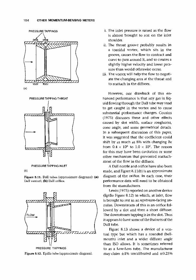
164 OTHER MOMENTUM-SENSING METERS
PRESSURE TAPPINGS
(a)
PRESSURE TAPPING-THROAT
x// /////// / V / / / / / / / / / / / /
PRESSURE TAPPING-INLET
(b)
Figure 8.11. Dall tubes (approximate diagrams): (a)Dall venturi; (b) Dall orifice.
f FLOW
r///////// . 1\ y V/ / / / / / / / / / / / / /7m—PRESSURE TAPPINGS
Figure 8.12. Epiflo tube (approximate diagram).
i. The inlet pressure is raised as the flowis almost brought to rest on the inletshoulder.
ii. The throat groove probably results ina toroidal vortex, which sits in thegroove, causes the flow to contract andcurve to pass around it, and so creates aslightly higher velocity and lower pres-sure than would otherwise occur.
iii. The vortex will help the flow to negoti-ate the changing area at the throat andto reattach in the diffuser.
However, one drawback of this en-hanced performance is that any gas in liq-uid flowing through the Dall tube may tendto get caught in the vortex and to causesubstantial performance changes. Cousins(1975) discusses these and other effectscaused by slot width, surface roughness,cone angle, and some geometrical details.In a subsequent discussion of this paper,it was suggested that the coefficient couldshift by as much as 8% with changing Refrom 0.4 x 10⁶ to 1.0 x 10⁶. The reasonfor this may have been cavitation or someother mechanism that prevented reattach-ment of the flow in the diffuser.
A Dall nozzle and orifice have also beenmade, and Figure 8.11(b) is an approximatediagram of the orifice. In each case, theirperformance data will need to be obtainedfrom the manufacturer.
Lewis (1975) reported on another device(Epiflo Figure 8.12) in which, at inlet, flowis brought to rest in an upstream-facing an-nulus. Downstream of this is an orifice fol-lowed by a slot and then a short diffuser.The downstream tapping is in the slot. Thusit appears to have some of the features of theDall tube.
Figure 8.13 shows a device of a ven-turi type but which has a rounded (bell-mouth) inlet and a wider diffuser anglethan ISO allows. It is sometimes referredto as a Low-Loss tube. The manufacturermay claim ±1% uncalibrated and ±0.25%

8.7 WEDGE AND V-CONE DESIGNS 165
calibrated with a repeatability of ±0.1% anda turndown of 10:1. Sizes range from 13 to1,200 mm. Installation is claimed to require12D upstream and 2D downstream for allbut partially shut valves and elbows in dif-ferent planes.
Vincent Gentile, Jr., described a tubewhich, in one form, is illustrated inFigure 8.14 and is known as a Gentile tube.It is claimed that it differs from other dif-ferential devices in that the pressure differ-ence is due to dynamic rather than staticpressures. It is also reversible (Scott 1982).
8.7 WEDGE AND V-CONEDESIGNS
Figure 8.15 shows a diagram of a wedge me-ter. They are designed with an asymmetricalconstriction, which may be positioned atthe top of the pipe, thus allowing any solidsto pass along the pipe. The constriction willresult in an increased velocity and reducedpressure. It is likely that a vena contractawill form downstream of the constriction
PRESSURE TAPPINGS
Figure 8.13. Low-Loss flow tube (approximate dia-gram).
PRESSURE TAPPINGS
1Figure 8.14. Gentile tube (approximate diagram).
so that the downstream tapping will sense the static pressure near the vena con-tracta (cf. Dall 1962 who refers to a segmental hump venturi).
It is, therefore, apparent that the orifice equation with a suitable coefficient willbe appropriate, but the size of the coefficient and its variation with Reynolds numberwill depend on the manufacturer's calibration data. Uncertainty after calibration of±0.5% is suggested.
Oguri (1988) suggested that a wedge flowmeter was suited to solid-liquid and gas-liquid flows. This is probably the reason for its preference over a segmental orificefor dirty or solids-bearing fluids - it is less likely to be damaged by them. It is claimedto have a long life without maintenance and without fouling. It may have a smaller
PRESSURE TAPPINGS
Figure 8.15. Wedge meter (approximate diagram).

166 OTHER MOMENTUM-SENSING METERS
pressure loss than the segmental orifice because of the slightly greater fairing of thewedge.
It is available in sizes from about 13 mm to about 600 mm and for a Reynoldsnumber range up from 500.
The V-shaped restriction to contract the flow is characterized by H/D (Ginesi1991). H is the height of the opening below the restriction (Figure 8.15). Thereare no critical dimensions or edge sharpness to be retained, and the element canwithstand wear and tends to keep clear of buildup due to the slanted upstream face.It is claimed to retain a square law down to about Re = 500, regardless of the state ofthe flow (laminar, transition, or turbulent). With few published recommendationsand no standardized geometry, the meter has to be calibrated, and suggestions of0.5% uncertainty have been made. For Re < 500, the calibration should be on afluid of the correct viscosity. The nonclogging feature with the low-flow capabilityand ruggedness have made this a realistic choice for fluids such as dewatered sludge,black liquor, coal, flyash, and taconite slurries. Ginesi claims that it is less sensitiveto installation than other differential pressure meters. The worst case reported byhim, 1.74%, was with three short radius bends in different planes at 5D upstream.To eliminate deviation, 20D is claimed as sufficient.
The commercial device may be offered as a wedge that can be inserted in schedule40 pipes of small sizes. The manufacturer may supply a mounting tube, constructedto allow direct connection to a pressure transducer, into which upstream and down-stream lengths can be screwed. With calibration ±0.5 to ±0.75% of rate is claimedwith repeatability of order ±0.2%. Materials are stainless and PVC, the latter as awafer design. It may also be available as a spool piece. The pressure tappings arepresumably symmetrical because the device is claimed as bidirectional. An elementis offered for water and gas with similar performance. H/D is in the range 0.2-0.5(Figure 8.15).
The V-cone meter (venturi cone, which may also be referred to as a McCrometertube) was introduced in the late 1980s and uses a conical flow restriction centrallymounted in the metering tube (Ginesi 1991, cf. Ginesi 1990; Figure 8.16). Pres-sure difference is measured across the cone. The beta ratio is equivalent to theopen flow area of the orifice, but a wider range is possible for the V-cone. Sizesrange from lines of 1-16 in. (25-400 mm), it has good rangeability, and it has re-sistance to wear, is insensitive to vibration, and is suitable for dirty liquids andgases.
It is claimed to have a turndown of 25:1 or more, presumably by using twopressure transducers, with uncertainty of better than 0.5% of rate and repeatabilitybetter than 0.1%. The differential pressure is measured between an upstream tappingand the trailing face of the cone. Ifft (1996) appears to claim that for a p = 0.5,the performance was ±0.5%, and even with a gate valve 0-50% closed and otherconfigurations, shifts were limited to 2%.
It is claimed 3D or less installation length upstream of the spool piece and 3Dto 5D downstream results in minimal installation effects. This is explained by thesuggestion that the profile entering the meter is flattened by the cone. The effectof a distorted profile on the upstream tapping is not mentioned. Ifft and Mikklesen(1993) suggested that a single elbow and double out-of-plane elbows with R/D =1.5had little or no effect (cf. Prahu et al. 1996).

8.8 DIFFERENTIAL DEVICES WITH A FLOW MEASUREMENT MECHANISM IN THE BYPASS 167
PRESSURE TAPPINGShigh low
highlow
PRESSURE TAPPINGS
Figure 8.16. V-cone meter (reproduced with permission of McCrometer, Inc., Hemet, CA).
8.8 DIFFERENTIAL DEVICES WITH A FLOW MEASUREMENTMECHANISM IN THE BYPASS
The pressure difference created across an orifice can be used to create a bypass flow,which in turn can be measured by some other flowmeter. One which has been usedis a small Pelton wheel. The jet created by the bypass impacts on the wheel, causingit to rotate and allowing the ferrites in the blades to cause pulses in the sensing coil.Claims are for ± 1 % of full scale on linearity or ±0.5% with 40:1 turndown usinglinearizing electronics and repeatability ±0.25% for 90% of range.
The oscillating vane meter uses an orifice with the vane in the orifice structureas a bypass (cf. Ginesi 1991). It may be available as a wafer design to go betweenflanges. The flow through the orifice creates a pressure drop that causes flow throughthe oscillating vane. The orifice appears to be concentric apart from one segmen-tal region in which the vane is situated. An electric pickup or proximity switchsenses the oscillation. Turndown is claimed as 10:1, with an uncertainty of ±0.5%of rate and a repeatability of ±0.2%. The meter is for liquid applications. Sizes are

168 OTHER MOMENTUM-SENSING METERS
from 25 to 76 mm (1-3 in.). Flow range is from 1.4 to 218 m3/h (5-800 gal/min)with a temperature range of about -25 to 100°C and pressure up to 21 bar. In-stallation recommendations are compared here with those for an orifice plate with0 = 0.3:
Oscillating OrificeVane /3 = 0.3
(Upstream/Downstream)Single bend 10/5 10/5Two bends in same plane 15/5 16/5Two bends in perpendicular planes 20/5 34/5Reducer 10/5 5/5Control valve 30/5 —Straightener 5/5 —
Some of the claims give cause for caution when compared with the orifice values.Other bypass elements used with differential meters are variable area, thermal,
and fluidic (Boucher et al. 1991). By including a secondary orifice in series with thebypass, the flow in each should be approximately proportional.
8.9 SLOTTED ORIFICE PLATE
Morrison et al. (1994a, b) suggested using an orifice that had radial slots arranged ontwo rings instead of a single central hole. The inner ring of slots extended from about0.1R to about 0.45R, and the outer extended from about 0.55R to about 0.9R. Therewere 8 slots in the inner ring and 24 in the outer, making an effective /3 = 0.43.They concluded from tests in a 50.8-mm line that the slotted orifice is less sensi-tive to upstream flow conditions than a standard orifice of the same effective betaratio.
8.10 PIPEWORK FEATURES - INLETS
If a well-formed inlet is provided to a pipe from a stilling tank or large gas vessel,then the pressure drop from the tank or vessel into the pipe can be used to obtainthe flow rate. Equation (6.1) is simplified since fi = 0, the flow coming from a large,essentially still, container, and so E = 1. The coefficient is also very close to unity.
The Shell Flowmeter Engineering Handbook (Danen 1985) gives values for the coef-ficient. The volumetric flow rate will be given by
qv = C(7t/4)dZy/2Ap/p (8.3)
where d is the throat diameter (at the downstream tapping) and may equal D, thepipe diameter downstream; Ap is the differential pressure between inlet and throat;and p is the density. The coefficients of discharge for various designs may be ob-tained from the Shell Flowmeter Engineering Handbook (Danen 1985). For example,

8 .11 PIPEWORK FEATURES - BEND OR ELBOW USED AS A METER 169
for a well-formed bell-mouth intake (cf. Fig-ure 8.17), the values of C may be
Re number 5 x 10³ 104 105 3 x 10⁵
C 0.914 0.940 0.987 0.991
The flow rate can be obtained from thesevalues and dimensions. The use of such aninlet will clearly depend on the condition ofthe installation and the upstream flow. Thelatter should be undisturbed and have hadsufficient stilling time. Even so, the methodshould be used with caution.
Ito et al. (1985) obtained values of about0.95 at Re = 20,000 to nearly 0.99 at Re =600,000, and also gave a useful list of references.
FLOW
PRESSURETAPPING
Figure 8.17. Bell-mouth intake.
8.11 PIPEWORK FEATURES - BEND OR ELBOW USEDAS A METER
In Chapter 4, the elbow meter is described as an additional means of in situ calibra-tion. However, Xu-bin (1993) reported that the device is widely used in China forthe measurement of primary coolant flows in pressurized water reactors, and that ithas also been used for measurement of steam, gases, clean liquids, slurries, sludges,and corrosive liquids. Xu-bin also points out that it is easy to install and maintain,can cope with large pipe sizes, and is less prone to damage.
Bean (1971) gives a full derivation of the relationship between pressure and flow.Here we give a simple derivation, which results in the same answer. Figure 8.18 showsthe geometry of the bend meter. If we make the grossly simplifying assumptionsthat
• V is uniform across the bend (clearly thisis not the case and there will be flow pro-file and secondary velocity effects as theflow negotiates the bend) and
• V2/R is the centrifugal acceleration forall the fluid in the bend (it won't be sincethe radius of each fluid element differs,and their velocities differ)
we can write that (Figure 8.18)
Force across the bend on unit area= Mass of fluid of unit cross-section
x Acceleration
PRESSURE TAPPINGPo
orV2/R (8.4) Figure 8.18. Bend used as a flowmeter.

170 OTHER MOMENTUM-SENSING METERS
Thus
V=/P (8.5)y D p
We are interested in the volumetric flow, and we introduce a flow coefficient toallow for the approximations to real flow. We obtain
(8.6)
Bean gave the coefficient as
K = l -6 .5 /VRe (8.7)
for 104 < Re < 106 and R/D > 1.25 and suggested that an uncertainty of ±4%should be allowed for. (Note that there appears to be a disagreement with Xu-bin'sequations.)
The use of pipe bends is also explained in the Shell Flowmeter Engineering Handbook(Danen 1985) where the coefficient includes the y/R/D. y/R/D for a normal 100-mmshort radius bend schedule 40 is approximately unity (Danen 1985).
This method should be used with extreme caution because the condition of thebend will be unknown and the uncertainty is unlikely to be as good as 4%.
8.12 AVERAGING PITOT
The Annubar was claimed to be the first averaging pitot (Britton and Mesnard 1982),but many others have followed. The averaging pitot is, strictly, neither averaging norpitot. In Chapter 18 we shall discuss pitot tubes, which are tubes coaxial with theflow. Although the averaging pitot has a series of upstream-facing holes, they are un-likely to provide a true average of the axial velocities across the pipe. The averagingpitot consists of a bar that spans the pipe and has holes facing upstream and down-stream [Figure 8.19(a)]. It is claimed to cope with disturbed profiles due to upstreamfittings. The flow will be brought to rest locally on the leading edge of the bar andat the upstream holes unless interconnecting flows occur. The resulting pressures ineach of the holes, which will approach the local stagnation pressures, will be linkedby the manifold that runs inside the bar. The rear-facing hole or holes will experiencea pressure that approximates to the static pressure in the flow. These two pressures,the approximate average stagnation and the approximate static, are then carriedby the internal tubes out of the bar and into a suitable pressure transducer wherethe pressure difference pu — pa will be calibrated against the velocity. Essentially, weassume that this pressure difference will approximate to the dynamic pressure thatwas obtained from Equation (2.10). The calculation of the actual upstream-sensedpressure will depend on internal flows in the connecting manifold from the cen-ter holes with higher stagnation pressure to, and possibly out of, the holes nearerthe pipe wall where the stagnation pressure will be lower. In addition, the squaredrelationship
&P=\pV2 (8.8)

8.12 AVERAGING PITOT 171
PRESSURE TAPPINGS
HIGHPRESSURESENSINGPORTS
FLOW
HIGHPRESSURESENSINGPORTS
LOWPRESSURESENSINGPORT(S)
(b)
Figure 8.19. Averaging pitot tube/bar: (a) Diagram of a typical meter; (b) Cross-sections ofvarious designs.
may result in an underweighting of the outer pressures where most of the flow passes.Calculation may suggest that the bar is a near-centerline measurement device withcorrection for profile shape from the outer tappings.
Figure 8.19(b) shows some of the cross-sections of the commercially availablebars. Because flow around a circular cylinder has a changing flow pattern dependingon the boundary layer, other shapes have been used to create a less varying pattern.Britton and Mesnard (1982) gave data comparing round- and diamond-shaped sen-sors, which clearly demonstrated the benefit of the latter over the former. While thecoefficient for the round cylinders varied by about 10% for a Reynolds number rangeof 2 x 10⁵ to 106, the diamond cylinder varied by about 2%. The final version of thecross-section for manufacture was a square section with flattened corners set so thatit presented a corner to the flow direction. In addition to the coefficient, a blockagefactor that allows for the reduced pipe cross-section at the probe is required. Theyclaimed a measurement uncertainty of ±1% and a repeatability of ±0.1%. It hasbeen suggested that a hexagonal bar with faces perpendicular to the flow overcomesthe problem of a circular bar, in forcing the flow separation at the edge vertices, aswell as the fabrication problem of diamonds and ellipses, which require a weld atthe pipe entry point. By using a hexagon, if necessary just at the actual taps, theintegrity of a round bar is retained. No doubt different manufacturers will have theirown reasons for cross-sectional superiority! The cross-sectional dimension of the barmay be in the range 10-50 mm.

172 OTHER MOMENTUM-SENSING METERS
Typical performance claims for these devices are ±1% of reading with ±0.1%repeatability for turndown of 10:1 or more and they are suitable for pipe sizes of25 mm (1 in.) to 12 m (about 40 ft). Manufacturers should be consulted on flowranges. Flows of 10-30,000 m3/h for liquids and 200-600,000 m3/h for gases maybe possible. Materials are stainless steel, Monel, Hastelloy, titanium, Inconel, PVDF,etc. Temperature range may be from —100 to 450°C, and pressure may be up to 70bar for some designs. It is claimed by some manufacturers that installation shouldbe with similar constraints to those for the orifice plate, and the connections shouldalso be similar to avoid condensation problems, etc. However, if we compare someclaims, we obtain the following:
Single bendTwo bends in
same planeTwo bends in
perpendicularplanes
ReducerExpanderValve*
0.2Orifice, (5
0.5 0.65(Upstream/Downstream)
10/4
14/4
34/45/4
16/418/4
14/6
20/6
40/66/6
18/622/6
22/7
32/7
54/711/725/728/7
Manufacturers
A BC (WorstCase)
(Upstream/Downstream)
7/3
9/3
17/47/37/3
24/3
24/4
11/4
—
9/49/4
27/4
10/5
15/5
28/510/510/528/5
These results suggest that, in the absence of clear guidance from the manufac-turer, taking the spacing for an orifice with p = 0.65 may be the wisest precaution.It should be remembered that the accuracy of any insertion device is subject to theuncertainty with which the pipe cross-sectional area can be measured. In the caseof averaging-pitots, there is a blockage caused by the bar, the effects of which mustbe obtained from calibration.
It is not clear how manufacturers overcome the uncertainty of the pipe ID andcross-section into which these devices are inserted. If installation of the pipe and barare at the same time, no doubt this measurement will be possible. The manufacturerwill then, only, need to know the allowance for blockage caused by the bar. However,if the pipe is in position, the measurement is considerably more problematic.
In some cases, it is possible that these devices may also create vortex shedding,a phenomenon that we shall encounter and use in the vortex-shedding flowmeter.Unfortunately, such shedding causes lateral forces on the bar and, if these are closeto the natural frequency of the bar, may cause vibrations of an unacceptable level.The manufacturer should be asked about this when considering such a device.
We shall discuss pitot tubes in Chapter 18 and shall find a very different shapeddevice. Cutler (1982), in a letter commenting on averaging-pitots, questions whethermultihole sensors do, in fact, generate an average differential pressure. Cutler madethe important point that, for fully developed flow profiles, a single-point mea-surement may suffice. We show in Chapter 2 that one measurement at about
* Orifice distances are based on a fully open globe valve.

8.13 LAMINAR OR VISCOUS FLOWMETERS 173
three-quarters radius will suffice for turbulent profiles. He gives an example of adevice consisting of upstream pointing and downstream pointing tubes.
A meter of this type has been marketed as a flow/no-flow indicator. Impact(upstream-facing) and suction (downstream-facing) ports supply a differential pres-sure that is displayed on a gauge attached to the pipe or may be used to obtain anindication of flow rate via differential pressure measurement.
8.13 LAMINAR OR VISCOUS FLOWMETERS
The viscous flowmeter for gases uses very small flow passages so that the pressuredrop is due to the viscous as opposed to the inertial losses and thus is proportional tothe flow rate. The reader is also referred to Chapter 15 where capillary thermal massflowmeters are described. These are frequently used in conjunction with a laminarflow bypass for higher flow rates. The design with differential pressure measure-ment appears to have been developed to measure gas flows for research into internalcombustion engines where there is a high level of pulsation and unsteadiness. As ob-served in Chapter 5, pulsation causes an overestimate of the flow if an orifice meter isused. The research engineers, presumably, realized that if the flow behavior could bedominated by viscous effects, the mean differential pressure across such an elementwould be proportional to the mean flow without errors due to a squared term.
The laminar flow in a circular tube can be shown to obey the equation (Baker1996)
1 ^ (8.9)K }
V=8 4/xL
where V is the mean velocity in the tube, Ap is the pressure drop along the tube,D is the diameter of the tube, /x is the dynamic viscosity, and L is the length of thetube. From this, we obtain the volumetric flow rate
In practice, we shall probably need to include, for a particular device, a calibra-tion coefficient C. For very small flow passages viscous effects ensure that, for mostpractical purposes, the equation will be valid for time-varying flows.
Figure 8.20 is a diagram of such a device with a laminar flow element throughwhich the flow passes, and with pressure measured in the upstream inlet chamberand in the downstream chamber.
Flow ranges for such devices are claimed to be from 0-2 ml/min to 0-2,0001/minwith a pressure difference up to about 10 mm H2O and a Reynolds number of about500. The meter is designed to be unaffected by installation and pulsation. Turndownof 20:1 or, with a mass flow computer, of 100:1 are claimed.
It is claimed to be suitable for any dry, clean gas. Calibration is claimed to 2% ofreading for 100:1 turndown with 0.2% repeatability and pressure in the range 0-7bar. Construction is of aluminum, brass, and epoxy. The design allows capacity tobe changed by altering the number of parallel passages.

174 OTHER MOMENTUM-SENSING METERS
PRESSURETAPPINGS
Figure 8.20. Diagrams of a viscous flowmeter.
Weigand (1994) referred to the Hagan-Poiseuille law (Poiseuille 1842) for flow ina capillary
Ap = Aqv/jLL/D4 + Bpql (8.11)
where A and B are constants, L is the length of the capillary, and D is its diameter.Other symbols have usual meaning.
Stone and Wright (1994) gave consideration to this meter and obtained the firstterm in Equation (8.11) and accounted for the second term:
a. due to entry length effects, which introduced onto Equation (8.10) a factor of(1 + QRe) where Cx ~ 0.03;
b. due to entry and exit losses, which they estimated as being of order 0.6% of totalpressure drop;
c. due to compressibility of the gas (Fanno line cf. Baker 1996) giving an error ofabout 1%.
If B is small compared with A and L/D4 is large, Equation (8.11) becomes
Ap = A'tiqy (8.12)
where A = AL/D4 (Bean 1971). This is essentially Equation (8.10) in an alternativeform. If we include the factor in (a), we obtain
(8.13)
which is similar in form to the equation obtained by Jones (1992) except that Jonesalso had a negative constant term.
Weigand claimed that the laminar flow elements that he describes can oper-ate over turndown ratios of up to 100:1. The main requirement is that viscosity isknown. The laminar flow element (LFE) consists of a housing and capillary element.The housing of stainless steel or aluminum provides inlet and outlet connections,structural support, and connections (e.g., to measure differential pressure). The cap-illary element may consist of one capillary tube with internal diameter as small as0.228 mm, a bundle of tubes, or a matrix array consisting of a series of triangularpassages made from 0.025-mm stainless steel stock and triangles with dimensionsof 0.58 mm or less. The length of the capillaries were 76 mm (25 mm for the largest

8.13 LAMINAR OR VISCOUS FLOWMETERS 175
AVV
(a) X X \\\\W\\\\V I
0.48 mm
-1
ACTUAL-PREDICTEDPRESSURE DIFFERENCE
AS A PERCENTAGEOF MAXIMUM Ap
EQ. (8.12)
,°EQ. (8.11)
100%(max)
FLOW RATE
(b) - 2 h
Figure 8.21. Test of viscous flowmeter (after Stone and Wright 1994): (a) Sectionthrough flow passages of meter; (b) Comparison between experimental data forpressure drop and equations of the form of Equation (8.11) (o) and Equation(8.12) (x). Maximum flow rate was about 32 1/s, and maximum Ap was about250 mm water.
devices and maximum flow rates to reduce pressure loss) and were rigidly held toensure geometric integrity and consequent repeatability. The 1.5-mm-diameter sens-ing ports are at the inlet and outlet and within 1.5 mm of the capillary element. Thedifferential pressure is usually less than 254 mm water. Single tubes are used for 0-5cm3/min up to 0-230 cm3/min. Bundles are used up to 1,300 cm3/min, and arrays,up to 425 m3/min. The normalized flow equation is given as
SCFM = ACFM/xg//xstd (8.14)
where SCFM is the standardized flow rate, ACFM is the actual flow rate from calibra-tion, /xg is the viscosity of the calibration gas at flowing conditions, and >std is theviscosity of the reference gas at standard conditions.
The entrance and exit of the capillary cause a slight nonlinearity. Repeatabilityis claimed as of order ±0.1%. Mass can be obtained using the density. For moistair, there is a humidity correction. Provided the temperature is less than about 26°Fand the relative humidity less than 80%, the correction is less than 0.4%. The meter

176 OTHER MOMENTUM-SENSING METERS
should be kept as warm as the flowing air. By combining temperature measurement,pressure measurement, and differential pressure measurement and using a micro-processor, gas mass flow rate is obtained. An uncertainty of ±1% of reading for 10:1turndown is claimed to be achievable.
Abe and Yoshinaga (1991) also described what appears to be essentially a lami-nar flowmeter with etoile-like resistors but with the center blocked. Their slits wererecommended to be 0.2 mm wide and 40-60 mm long. With two in parallel, theyclaimed flow rates up to about 0.5 x 10~3 m3/s were possible, but nonlinearity ap-peared to set in below this figure. The device may be used as a flowmeter or a meansto measure viscosity.
Stone and Wright (1994) tested a meter with passages as shown in Figure 8.21 (a)with length 76.2 mm, about 18,000 passages and a flow area of 3507 mm2. Thehydraulic mean diameter was 0.347 mm, and the mean velocity at rated flow was 1.73m/s. Figure 8.21 (b) shows the flowmeter characteristic compared with a quadraticassumption as in Equation (8.11) and a linear assumption as in Equation (8.12). Bothcurves were obtained using regression analysis and not through evaluation of theconstants.
8.14 CHAPTER CONCLUSIONS
This chapter has been used to "sweep up" a number of types of meter, among whichthe variable area meter is the most common. The great benefit of the transparent-tube designs of the variable area meter is the immediate visual reassurance that flowof a certain level is taking place. However, in many applications, a metal tube maybe considered necessary for safety reasons. Recent work has started to analyze theflow and to identify reasons for the instability that has been observed since the firstuse of the meter. There may be value in pursuing these studies further to provide ananswer to the reasons for limits of accuracy for the meter:
• Does upstream disturbance including swirl actually affect performance?• Why is it necessary to quote an uncertainty as a percentage of full flow?• Does turbulence level affect the meter reading?
Many of the devices depend on proprietary information on performance. Mylaboratory did tests on one of them under certain flow conditions, but even so Iam not able to provide the data here because it is commercially confidential. Theuser is, therefore, heavily dependent on the information provided by the manu-facturer.
The averaging-pitots clearly have a useful role where a full-bore meter is notpossible, but whether the claims for installed accuracy are reproduced in practice isdependent mainly on manufacturers' data.
It seems likely that devices such as those in this chapter that use one or other of
• contoured tube walls,• various shapes of insert, and• existing pipe features

8.A.1 SOME HISTORY 177
will continue to have a place. Several of the designs described have been introducedrelatively recently.
If a manufacturer is considering the introduction of new designs, the user willbe dependent on manufacturer's data for most of the designs that fall outside a stan-dard's specification. The quality of the manufacturer's total operation will, therefore,be a key consideration. The effect of installation should be plausible compared withsimilar devices from elsewhere. The biggest uncertainty will be in the special condi-tions that are unforeseen: small traces of gas in a liquid becoming trapped in flowvortices, deposition of small quantities of a solid or liquid film, and materials prob-lems. Increasingly, however, the question will need to be asked, "Is there a linearmeter that would be more appropriate?"
APPENDIX 8.A
History, Equations, and Accuracy Classesfor the VA Meter
8.A.1 SOME HISTORY
In 1873, G. F. Deacon produced a design that resembled a variable area meter. Thiswas very similar to an earlier device patented in 1868 and made by E. A. Chamberoyof Paris (Coleman 1956). Something similar was devised by Sir J. Alfred Ewing(1924-5) in about 1876 and was initially known as the Ewing flowmeter. Furtherexperiments were carried out by Awbery and Griffiths (1926-7). They found thatthe float, if a ball, started chattering at high flows and caused an overreading. Threesolutions were suggested:
i. Inclining the tube so that the ball rolled on the wall. This was Ewing's preferredsolution,
ii. Using a float of a different shape. Awbery and Griffiths (1926-7) mentioned thatthe meter used a cylindrical float with helical channels to cause slow rotation,
iii. Stretching a fine wire along the tube close to the wall, to prevent the chatteringmotion (Advisory Committee on Aeronautics 1916-17). Awbery and Griffithsverified this in their observations.
One possible reason for this instability (Leder 1996) is a saddle point (free stag-nation point) that forms in the wake downstream of the ball and off-axis and thatrotates and induces a large scale rotating helical vortex together with small scaleturbulence motions.
Ewing suggested that the range of the instrument could be extended by incor-porating more than one float. The largest would be on top and would record lowflows, and the smaller ones underneath would rise when the flow rate was sufficient.Ewing also used a dye trace to show the nature of the flow. An alternative could beto have two floats of similar size but with the top one of lower density.

178 OTHER MOMENTUM-SENSING METERS
Awbery and Griffiths showed that their experimental results collapsed onto asingle curve for a given diameter ratio of D/d, where D is the diameter of the tubeat a certain height, and d is the diameter of the ball. They plotted log[qvD/(D2 — d2)]against \og[d3(pf — p)/v2p], where qv is the volumetric flow rate, p is the densityof the fluid, pt is the density of the float, and v is the kinematic viscosity of thefluid.
British Patent 2428 granted to G. Joslin of Colchester (1879) covered a device forascertaining rate of consumption of gas, which resembles a VA meter, and this wasfollowed in 1908 by a patent granted to K. Kuppers of Aachen for a tube and floatvery similar to Joslin's. Felix Meyer of Aachen obtained the patent and started man-ufacturing the tubes. In 1921 Trost Brothers Ltd. of England took up Meyer's agencyfor the United Kingdom, and in 1931 Schutte and Koerting secured the manufactur-ing rights for the United States. Coleman (1956) gave a very useful historical reviewfrom which some of these notes are taken.
Head (1946) refers to a downdraught instrument in which the float is lighterthan the fluid.
8.A.2 EQUATIONS
The basic theory of the flowmeter depends on the upthrust on the float resultingfrom the pressure loss across it
where pi and p2 are the upstream and downstream pressures, K is a loss coefficient,p is the density and V is the velocity in the annular passage past the float. Replacingvelocity by volumetric flow rate qv such that
V = qy/A2 (8.A.2)
where A2 is the annular area around the float, we obtain
Pi-p2 = K11pq2/A2 (8.A.3)
This equation assumes that the dynamic head at inlet is negligible, and that thepressure difference across the float is caused by the loss of the dynamic head down-stream of the float. Dijstelbergen (1964) uses a contraction coefficient Cc for the ratioMl Ax, where Ax is the area of the tapering tube at height x.
The immersed weight of the float is given by
W=Vf(Pi-p)g (8.A.4)
where Vf is the volume of the float, pf is the density of the material of the float, andg is the acceleration due to gravity. Thus, the balance is given by
- p)g (8.A.5)
where Af is the maximum cross-sectional area of the float.

8.A.2 EQUATIONS 179
This is usually rewritten as
Cc 2Vf (pt-p)g (8.A.6)
with l/y/K replaced by C (e.g., Martin 1949,Coleman 1956; cf. Head 1946-7).
Coleman (1956) gave values of C forthree float shapes (Figure 8.A.I), which sug-gested that at full flow the value of C rangedfrom 0.6 for a float of low Re sensitivityto about unity. The plots also showed adecrease in C at low flow rates, and thiswould broadly reflect the fact that the losscoefficient for an orifice increases with re-duced Re (Miller 1990). Coleman also plot-ted the effect of viscosity on the variousfloat shapes and confirmed the implicationsof Figure 8.A.I, that the plumb-bob is themost viscosity dependent.
Schoenborn and Colburn (1939) gave acurve of C against Re/C, where Re is theReynolds number based on Deq. They calledit the equivalent diameter but defined itas the difference between D and d. Thiscurve is reproduced in Figure 8.A.2. It wasobtained for a large high pressure designusing a steel tube with extension rod ob-servable through a graduated glass window.This curve could be used as a first approxi-mation if no other is available. They used abalance of forces of the weight of the float inliquid to the upward force due to the pres-sure reduction across the float to providethe basis for their experimental correlation.They also noted that the curve for largemeters appeared to be less fluid-dependentthan for smaller instruments.
Although it may be difficult to predictflow rates, it is possible to convert fromone fluid to another at the same read-ing. Schoenborn and Colburn (1939) gavean equation similar to that given by ISA(1961b):
(8.A.7)
1.0
0.5
10 102 10° 104 Re 105
1.0
0.5
10 104 Re 105
1.0
0.5
10 10° 104 Re 105
Figure 8.A.I. Effect of float shape on flow coefficient(after Coleman 1956).
1.0
0.5
10 Re/C 10
Figure 8.A.2. Plot of C against Re/C for a typical vari-able area meter (after Schoenborn and Colburn 1939).

180 OTHER MOMENTUM-SENSING METERS
I.UO
1.02
1.01
1.00
0.99
0.98
0P7
/(Pf-P2)p2- \ ( P , - P I > P I
- — - ^ ^ ^
— ^ ^ ^
float s.g.
7 . 9 ^ / ^
^ ^ ^ ^ ^ — ^ ^ ^ 1.44
SPECIFICGRAVITY OF
METERED FLUIDi i i
0.68 0.69 0.70 0.71 0.72 0.73 0.74 0.75 0.76s.g. FOR
CALIBRATION FLUID
Figure 8.A.3. Density compensation float comparison curves (after Coleman1956).
The difference is that ISA (1961b) omits C2/C1, thereby making the assumptionthat the ratio is unity. Coleman (1956) also used this equation with C2/C1 equalto unity, noting that variation of viscosity is ignored. He referred to the fact that ifEquation (8.A.6) is rewritten for mass flow rate and differentiated for variation influid density, it can be shown that a float density, of twice the fluid density gives azero change and, therefore, is least sensitive to variation in density (cf. Head 1946).Figure 8.A.3 shows values of the density correction factor with change of fluid densityand for various float densities, based on calibration for aviation gasoline of specificgravity 0.72. Head (1946) also raised the possibility that, with a downdraught design,the requirement from differentiating the volume flow equation of a float of zerodensity could be achieved approximately. Head also suggested that float automaticcompensation might be used to allow for temperature variation and other variables.Several authors have pointed out that the value of C is constant if /x/y/pipf — p) isconstant.
8.A.3 ACCURACY CLASSES
To define the accuracy of the variable area flowmeter, VDI/VDE 3513 (1978) recom-mended an accuracy class and divided the reading into two parts:
• First part is three-quarters of the actual flow rate M;• Second part is one-quarter of full-scale or upper range value E.
The summation error F in flow rate, in actual flow rate units, is then given by

8.A.3 ACCURACY CLASSES 181
where K is the accuracy class number selected from a range from 0.4 to 10. Forexample, taking a full-range flow of 100 units, the actual error will be
at full scale f | x 100 + i x 100^ - ^ - = K units
at 1/10 full scale (- x 10 + - x lOo) — = 0.325 K units\4 4 J 100
If we take a value for K of 2.5, then the error at full flow will be 2.5 units in 100units (2.5%), whereas at 1/10 full flow it will be 0.812 units in 10 units (8%).

CHAPTER S
Positive Displacement Flowmeters
9.1 INTRODUCTION
The material in this chapter is based on the paper by Baker and Morris (1985) onpositive displacement (PD) meters, which in turn has been updated with more re-cent industrial and published material and extended to gases. P.D. Baker's (1983)paper provided some additional useful information on these meters. The main typesof liquid meter were given by Barnes (1982), Hendrix (1982), Henke (1955), andGerrard (1979) (cf. Mankin 1955). The reader should refer to API (1992) and similardocuments.
At least four of the meter designs to be discussed have been around for over 100years. The nutating disk flowmeter for liquids was developed in 1850. The rotarypiston meter appeared in the late nineteenth century (Baker 1998).
The measurement of gas has depended, from an early date, on two types ofpositive displacement meter: the wet gas meter of high accuracy and credited toSamuel Clegg (1815), and the diaphragm meter of lower performance but greaterrange for which William Richards (1843) should take the credit.
9.1.1 BACKGROUND
The concept of carrying known volumes of fluid through a flowmeter is a short stepfrom the use of a discrete measure such as a bucket or measuring flask. Thus in eachof the designs described later, the flow enters a compartment that is as tightly sealedas is compatible with relative movement of adjacent components. A knowledge ofhow many of these compartments move through the flowmeter in one rotation ofthe shaft leads to a knowledge of the flow rate for a certain rotational speed. A sim-ple theory is developed in Appendix 9.A.I. Clearly every leakage path will reduceor increase the amount carried and cause an uncertainty in the measurement. Wecan make an approximation of the leakage flows in the simple model. In addition,pressure and temperature will distort the volume and may cause small errors, andwe may need to develop compensation for these. Compensation for pressure canbe provided in the form of a double-walled meter in which the precision-measuringchamber is unpressurized since the pressure is the same inside and out, and the pres-sure drop to the outside world is taken across the second and outer wall, the shape ofwhich will not affect the accuracy. The temperature compensation, if necessary, canbe incorporated into the calibration adjustment by a temperature-sensitive element.
Very often these devices provide a direct sales ticket that is produced by therotation of the meter and the starting and stopping of the flow. On the other hand,
182

9.1 INTRODUCTION 183
it is very difficult to make small adjustments as needed in calibration where thesignal is from a mechanical rotation. We, therefore, need to introduce complicatedmechanical calibrators where a frequency output is not acceptable. The combinationof mechanical counter and ticket machine can cause a substantial drag on the meterand may cause slippage errors in certain types of calibrators.
Many of the points made in this chapter relate primarily to liquid measurement,have some relevance to gases, and should be noted by those mainly interested in gasmeasurement.
9.1.2 QUALITATIVE DESCRIPTION OF OPERATION
The essential of any positive displacement meter, as indicated earlier, is that a discreteand well-defined portion of the fluid is carried from inlet to outlet without loss ormixing with the remainder of the fluid. This applies to all the fluid that passesthrough the meter. The skill and ingenuity of the designer is shown, therefore, inachieving this as simply and precisely as possible. If, for instance, we know thevolume of each compartment of a reciprocating pump, then knowing how manycylinder-full portions are transmitted in a revolution, we can relate the amountpassed to the speed or revolutions of the pump. This is essentially the principleof a metering pump. Taking this a step farther, we could reverse the reciprocatingpump. Instead of providing power externally to drive the pump, the fluid moves thepistons, and the valves ensure that each portion is transmitted, without loss, to theoutlet. Of course there will be some loss due to imperfect sealing between the pistonsand the cylinders, but provided this can be kept very small, we have the basis of avery accurate instrument. The reciprocating principle may not be satisfactory forhigh throughput meters, and so other designs have been devised. It will be easiestto explain the working of each in turn with respect to diagrams.
The theory of the device is worked out in Appendix 9.A.I. Here we need onlynote that the simplest equation of flow through such a device is
qv = Volume per revolution x Rotational speed — Leakage (9.1)
Leakage is unlikely to be a constant value for one revolution and is more likely tobe speed-dependent. The output from all meters is a rotating shaft, and this needs tobe related to the flow rate and total passed. If the shaft passes through the pressurecontainment of the meter, then a rotary-shaft-sealing arrangement will be needed.In one type of meter, an externally lubricated packing gland is used to isolate thedynamic shaft seal from the product (Baker 1983), thereby increasing the life of thepacking gland. The external lubricant must, of course, be chemically compatiblewith the product being metered. In some cases, the problem is avoided by using amagnetic drive coupling.
In the past, calibration and transmission methods have tended to be by mecha-nical linkage. Such a linkage loads the rotor and may alter the characteristic of themeter. It is also difficult to design a mechanical system to adjust the calibration ofthe meter. Some ingenious methods have been adopted and will be described later inthe chapter, largely for historical interest and for those who have dealings with suchdevices that remain in service. Today the possibility of using electrical or optical

184 POSITIVE DISPLACEMENT FLOWMETERS
Inlet Outlet
Figure 9.1. Nutating disk meter (reproduced fromBaker and Morris 1985; with permission of theInstitute of Measurement and Control).
transmission and still retaining intrinsicsafety means that an output pulse train canbe used, and signals can be manipulatedelectronically.
9.2 PRINCIPAL DESIGNS OFLIQUID METERS
This section reviews the main designsand their special operational features and,
where possible, reviews the published information that is available about them.
Inlet
9 .2.1 NUTATING DISK METER
In the nutating disk meter (Figure 9.1), the disk is constrained by the central spheri-cal bearing and by the transmission to nutate. Nutation is a movement rather like aspinning top that is slowing down. The disk is prevented from rotating by a partitionseparating the inlet and outlet streams. The incoming flow causes the disk to nutateand in doing so the disk forms a closed compartment trapping a fixed volume of liq-uid. There are effectively two such compartments, one above and one below the disk.
The disk element has the shape of the planet Saturn. The important difference isthat the disk has a slit in its "rings/' which makes a close fit with a radial partition.Flow enters, say, under the disk on one side of the partition and causes the disk torise and fill the region under the disk, and so to nutate. When it has nutated halfa turn, the entry port becomes blocked by the disk, and the other entry port abovethe disk has started to allow fluid above the disk. At the same time, the exit portfor the liquid below the disk opens to discharge. Thus in terms of Equation (9.1),in one rotation, the cavity on one side of the disk is both filled and discharged. Itis unlikely that the leakage can be kept very small, and the overall accuracy is notexpected to be very high. Although rather difficult to describe, it is a simple meterof low cost, rugged and capable of uncertainty within ±1.5%. (Henke 1955).
Typical industrial designs, some of which may be for water flow measurement,may have a built-in filter. Claims for measurement uncertainty may be of order1% for flow rates of 10-100 1/min with minimum pressure of 0.1 bar, viscosity up
to 1,000 mPa, and temperature up to 80°C.Materials may be stainless steel, polypropy-lene, or ethylene-tetra-fluor-ethylene. Mod-ern designs may include a microcomputerto convert flow rate into the correct units.
9.2.2 OSCILLATING CIRCULARPISTON METER
The oscillating circular piston meter(Figure 9.2) is similar to the nutating diskmeter in that the rotation of the piston isconstrained by a partition, so that the pis-ton, in fact, rocks. Its center is constrained
Outlet
Figure 9.2. Oscillating circular piston meter (repro-duced from Baker and Morris 1985; with permissionof the Institute of Measurement and Control).

9.2 PRINCIPAL DESIGNS OF LIQUID METERS 185
FlutedRotors
Flow
(a)
MainRotorVanes
StationaryBlock
Flow
(b)
Secondsealingrotor
(C)
Figure 9.3. Multirotor meters: (a) Two rotor (re-produced from Baker and Morris 1985; with per-mission of the Institute of Measurement andControl); (b) Two rotor, main rotor has four vanes(reproduced from Baker and Morris 1985; withpermission of the Institute of Measurement andControl); (c) Multirotor: large rotor with twosmall rotors (after Baker 1983 and Baker 1989).
to move in a circle by the transmission so that the radius of the cavity is essentiallythe sum of the radii of the rotary piston and the circle on which its center moves.When the center of the rotary piston is at the top of its travel, the piston forms aclosed compartment with the cavity. One rotation of the shaft will cause the rotarypiston to return to its starting place and so to discharge the volume of one compart-ment. In some designs, the leakage may not be negligible. As well as use with water,these meters may be made in designs suitable for liquid foods and other nutritionalfluids (Anon. 1966a). Hamblett (1970) suggests that they can achieve a measurementuncertainty within ±0.25% for flow rates from 0.018 to 110 m3/n (4-25,000 gal/h).This accuracy is rather higher than would be expected. He also lists the various typesof registers and controls that are suitable for a range of applications.
9.2.3 MULTIROTOR METERSThere are several designs of meter with multiple rotors. Figure 9.3(a) has two rotorsthat seal against each other; each rotor carries liquid through the meter as it rotates.Figure 9.3(b) shows another two-rotor meter, but in this case the main rotor consistsof four vanes that form metering compartments. The second rotor is a sealing rotorthat returns the vanes to the inlet side of the meter. The second rotor may be two-or three-lobed, and its rotation will be precisely linked to that of the main rotor. Ittransmits a net fluid flow across the meter equal to the volume of the vane that itreturns to the inlet. The mechanism, its design and engineering, is complex and,unless manufactured to a very high standard of precision, may lead to high pressureloss and interference between rotors and housing. Figure 9.3(c) shows a design witha large rotor and two small rotors.
9.2.4 OVAL GEAR METERThe oval gear meter (Figure 9.4) is a special form of a multiple rotor meter in whicheach oval rotor is toothed, and sealing between the rotors is enhanced by the

186 POSITIVE DISPLACEMENT FLOWMETERS
Percent error+0.6
+0.3
0
-0.3
-0.6
(b)
Pressuredrop
0.50.4
bar 0.30,20.1
0
50% 100%
Figure 9.4. Oval gear meter: (a)Working principle (reproducedwith permission of Bopp andReuther); (b) Error curves for arange of viscosity values (afterHaar Messtechnik); (c) Typicalpressure drop for operating range(after Haar Messtechnik).
flowrate
(c)50% 100%
flowrate
resulting labyrinth. Each rotor transmits fluid from inlet to outlet and forms a closedcompartment when its major axis is aligned with the flow direction. The volumepassed per revolution of each rotor is four times the volume between the rotor andthe oval housing when the rotor is confining liquid [Figure 9.4(a)]. In place of theleakage paths between the rotors of multirotor meters, there will be, for this meter,extremely small leakage where the rotors mesh, and the tolerances for the othersurfaces are likely to be to a high standard, giving a very small value for the overallleakage.
Small examples of this device are found in oil-flow lines in hydraulic sys-tems, whereas larger high precision stainless steel versions are also available.They are claimed to have a low pressure drop, to have low maintenance, to beof simple construction, and to achieve accuracies within ±0.25% (Henke 1955).Meters are available with a stress-free measuring chamber for high pressure appli-cations.
The meter can be subject to viscosity variation. Figure 9.4(b) shows the error, andFigure 9.4(c) shows the pressure drop for a typical commercial design. Measurementuncertainty is in the range ±0.1-2%. Sizes are from 6 to 400 mm, with flow rangesfrom 0.1 1/m or less up to 1,200 m3/h, but many are for smaller flows. Turndownis of order 10:1 (Endress and Hauser 1989), and operation is possible with, andlargely unaffected by, viscosity in the range 0.4-20 cP. However, the possibility ofa calibration shift (of order 0.5%) should be checked with the manufacturer. Onemanufacturer suggests that operation is possible up to very high viscosities. Pressure

9.2 PRINCIPAL DESIGNS OF LIQUID METERS 187
loss is 0.5-1 bar, and pressure may be up to 40 bar or higher for certain designs, withtemperature up to 290°C.
Transmission may be through a permanent magnet coupling or through magnetsembedded in the oval wheels that generate a voltage in an external inductive sensor.Calibration gearing may also pass the output to a totalizing counter. Operation maybe bidirectional.
Materials may be, for the body, stainless steel, cast iron, or aluminum and, forthe gears, carbon steel, brass, or chemical-resistant plastic.
Applications are in adhesives and polymers, but also in many basic utility flowsin the water industry and in hydraulic test stands. One manufacturer includessolvents, paints, and adhesives; dispersions, polymerisates, and polycondensates;glucose and alcohols; organic and inorganic liquids; gasoline, fuel oils, lubricants,and raw and intermediate liquid products; and other liquid chemicals.
9.2.5 SLIDING VANE METERSSliding vane meters (Figure 9.5) are, probably, the most accurate of this family ofmeters. Closed metering compartments are created by means of sliding vanes thatmove out from a slotted rotor to meter the fluid through a passage of constant shape.The movement of the vanes is caused, in the example in Figure 9.5(a), by an internalstationary cam. The inside edges of the vanes have rollers that follow the cam. Thevanes are designed to have a small clearance on all fixed surfaces. The movement ofthe vanes, in the example of Figure 9.5(b), is achieved by an external cam, which theoutside edge of the blade, where it meets the end faces, follows. There is thereforesome surface contact, which can result in wear and a need for calibration checks.
The elaboration of Equation (9.1) in Appendix 9.A.I is focused on these devices.The measuring volume per revolution is essentially the volume between the twoconcentric cylinders, which make up the outer case and the rotating inner wheelwith vanes. It is reduced by the volume of the vanes themselves. These designs canbe highly accurate, and much of the following discussion is concerned with thelimits of accuracy. For instance, they are expected to measure with great precisionthe transfer of valuable liquids, controlled by agencies such as H.M. Customs andExcise (1995). Such precision is likely to be demonstrated by short-term repeatabi-lity, such as three successive measurements of 500 liters within 0.1%, and long-termrepeatability over a 6-month period within 0.15%.
Walles (1975) gave figures from his own tests indicating that these figures areachievable with this type [which he refers to as a rotary piston meter and, as shownby his illustration, is in our category of sliding vane meter, Figure 9.5(b)]. He dividedthe errors in a meter with a double-walled case into three classes - short, medium,and long term. Experimental tests with kerosene at the U.K. National Gas TurbineEstablishment, in which the flow was diverted into calibration vessels, suggestedthat the following figures were applicable: leakage, 0.005% of rated flow; short-termerrors, 0.005-0.05% for different flow rates (affected by environmental and fuel tem-peratures and hence by weather and conditions); medium-term errors, 0.05%; andlong-term errors, 0.2%. This gave a year-to-year repeatability of within 0.15%. Sys-tematic (long-term) errors (e.g., in calibration equipment) were difficult to estimatebut might be expected to add an additional 0.2% so that the absolute accuracy wasestimated at ±0.35%. Another paper (Walles and James 1985) suggested that the per-formance of positive displacement flowmeters can be represented by an ideal meter

188 POSITIVE DISPLACEMENT FLOWMETERS
CamMeasuringChamber
MeterHousing
BladeBearing
Rotorvanes (or blades)
measuringchamber
(c)
Figure 9.5. Sliding vane meter: (a) Smith type showing blade (vane) path (reproduced fromBaker 1983; with permission of the author); (b) Avery Hardoll type (after the manufacturer'sliterature); (c) VAF J5000 (reproduced with permission of VAF Instruments and Industrial FlowControl Ltd.).
of arbitrary but constant volume in parallel with a small leakage that is independentof flow rate.
Manufacturers claim very high performance in line with these published figuresof 0.1-0.3%. A repeatability of 0.01-0.05% for flow ranges from about 3 m3/h up to2,000 m3/h with turndown ratio of 20:1 and size range of 64-152 mm (2.5-6 in.)is typical. One penalty of this type of meter is its bulk and weight (60-136 kg). In

9.2 PRINCIPAL DESIGNS OF LIQUID METERS 189
some designs, the highest flow rates are achieved by ganging the meters togetherin a double or triple capsule. Pressure loss should be kept to within 70-100 kPa(10-15 psi) by suitable choice of meter size.
Materials may be cast iron for the bodies, and the rotors may be made of similarmaterials or other materials such as aluminum. The same is true for outer covers. Lowfriction ball bearings may be used. Static seals may be high nitrile, whereas dynamicseals may also be fluorocarbon. Working pressure is about 10 bar, and temperatureranges from about -25 to 100°C. Temperature changes cause less than 0.0015%/°C,which is small compared with the theoretical values due to selection of materials.The measuring chamber is fitted with pressure-balanced end covers to ensure thatthere is no pressure difference across the end covers of the measuring chamber andso to avoid distortion. Figure 9.5(c) shows a device that may also be available for 10-to 200-mm pipe bore sizes.
9.2.6 HELICAL ROTOR METER
Two radially pitched helical rotors trap liquid as it flows through the flowmeter caus-ing the rotors to rotate in the longitudinal plane (Figure 9.6). Flow through the meteris proportional to the rotational speed of the rotors. It can be used on high viscosityliquids, but increased slippage may occur with low viscosity flows and reduce theaccuracy. The rotors form a seal with each other and with the body of the flowmeterso that these parts must be manufactured to a high degree of precision. One man-ufacturer (Gerrard 1979) claimed that its positive displacement meter with helicalelements had an accuracy of ±0.5% over a 150:1 flow range and a repeatability of±0.1%. Performance of 0.1% rate uncertainty and 0.01% repeatability with low effectfrom viscosity are now claimed. Some designs may withstand pressures up to 230 bar,compensate for temperature changes, and allow the passage of small solids. The useof Equation (9.1) will require a knowledge of how many closed compartments thereare created by the two helical rotors and how many of them pass in one rotation.
One manufacturer confirms the precision level, suggesting that a higher pressurerating is possible, with maximum flow of about 13 m3/h, an operating temperatureup to about 290°C, and viscosity up to 106 cP.
Applications are to polymers and adhesives, fuel oils, lubricating oil, blending,hydraulic test stands, high viscosity, and thixotropic fluids. This type of meter hasalso been developed for multiphase flows in North Sea oil applications (Gold et al.1991).
Flow
Figure 9.6. Helical rotor meter (reproduced from Baker and Morris 1985; withpermission of the Institute of Measurement and Control).

190 POSITIVE DISPLACEMENT FLOWMETERS
Figure 9.7. Reciprocating piston meter (reproduced from Baker and Morris1985; with permission of the Institute of Measurement and Control).
9.2.7 RECIPROCATING PISTON METERSOne design in which four pistons trap liquid as it passes through the flowmeter isshown in Figure 9.7. The crankshaft rotates with a rotational speed proportional tothe flow through the meter. The liquid that passes through each cylinder in onerotation of the shaft is equal to the swept volume of the cylinder.
Meters of this type have high accuracy claims and may also have a high pressuredrop. The Aeroplane and Armament Experimental Establishment (Anon. 1966b)developed a three-cylinder meter for low flows. Accuracies of ±0.5% were quotedfor kerosene flows of 9-182 1/h (2-40 gal/h) with ±2% for gasoline at rates below32 1/h (7 gal/h). Increased slippage made high accuracy difficult to achieve at lowflows, particularly for less viscous liquids.
One commercial producer quotes up to 33 m3/h (120 gal/min) with ±0.5% ofreading and with an 1,800:1 turndown and another down to 11/h. Viscosity may bepossible up to 30,000 cP or greater and temperatures up to about 280°C. Magneticcouplings may be used to reduce drag and avoid a rotating seal.
Endress et al. (1989) mentioned accuracy of ±0.5 to 1% of rate, turndown of10:1, maximum differential pressure of 5 bar, diameter range of 25-100 mm, andmaximum pressure of 40 bar. Others may offer pressure ratings up to 200 bar.
Materials of construction may be predominantly stainless steel with seals ofViton, Teflon, neoprene, Nordel, Buna-N, etc. Filtration to 10 /xm may be required,and magnetic coupling may be appropriate.
Applications include gasoline pumps, pilot plants, chemical additives, engineand hydraulic test stands, fuel consumption analysis, blending and ratio control,and mercaptan odorant injection.
9.2.8 PRECISION GEAR FLOWMETERSFigure 9.8(a) shows an example of a commercial device. The spaces between the gearsand the chamber wall form the fluid transfer compartments. In this version, rotationis sensed by two electromagnetic sensors operating through a pressure-resistant andnonmagnetic element in the housing. Two sensors can be arranged to allow bet-ter resolution than one and to determine flow direction. Measurement uncertainty[Figure 9.8(b)] of ±0.1% rate is claimed. It is also claimed that rapid flow reversal canbe followed (e.g., 801/min in about 0.01 s). Meters for flow ranges of as low as 0.0011/min and as high as 1,000 1/min may be available with temperature ranges of -30to 150°C and pressure up to 300 bar or more. Figure 9.8(c) shows typical pressure

9.3 CALIBRATION, ENVIRONMENTAL COMPENSATION, AND OTHER FACTORS 191
1.05-cm3
1.045-
| 1.04
£1.035
| 1.03
> 1.025
1.02
+0.3%
0.3%
0 10 20 30
L/min
40 50 60 70 80Flow rate
(b)
Figure 9.8. Precision commercial gearmeter (courtesy Kracht, KT Hydraulic Sys-tems Ltd.): (a) Showing the gears, sen-sors, and preamplifier; (b) Typical uncer-tainty characteristic; (c) Typical pressureloss curves for various viscosities.
Viscosity (mmVsec)3000 1000 600 300
16 -14 -12 -10 -8 -K -
; :
0 -
/
/
/
/
1 y
/W
//? ///
4
/
y
z
y
^—
y
^^
y
y
y
yy
100
34
10
10 20 30 40 50 60 70 80
Rowrate — L /m in
(c)
losses for various viscosities. Plain bearings or ball bearings may be used dependingon the liquid monitored.
Applications may include gasoline, paraffin, kerosene, diesel, mineral oil, hy-draulic oil, ink, dyes, paint, greases, polyurethane, polyol-iso-cyanate, glue, paste,cream, resin, and wax. For the auto industry, applications are hydraulic systems, fuelconsumption, paint spraying, batch processes, adhesive coatings, hydraulics; and forthe chemical industry, applications are process plant, batching, leakage, and mixingratios.
At least one design is available using a servomotor to maintain zero pressuredrop across the meter (cf. Conrad and Trostmann 1981, Katz 1971 regardingservo-control).
9.3 CALIBRATION, ENVIRONMENTAL COMPENSATION,AND OTHER FACTORS RELATING TO THE ACCURACYOF LIQUID FLOWMETERS
This section is primarily concerned with sliding vane meters. It should be remem-bered that the drive from these meters, when mechanical, may have to be used on

192 POSITIVE DISPLACEMENT FLOWMETERS
Leakage%
Bypass
0.8
0.6
0.4
0.2
Mechanicalfriction
20 40 60 80URV
Figure 9.9. Typical effect on accuracy of leakage due to mechanical friction fora sliding vane positive displacement meter (reproduced from Baker 1983; withpermission of the author).
a mechanical calibration device that loads the drive and causes a drag on the rotors.Manufacturers will clearly aim to reduce this as far as possible by the use of lowfriction ball bearings, etc. The mechanical methods of calibration adjustment arediscussed first, and the theory behind them is elaborated in Appendix 9.A.5. Baker(1983) gave the characteristics of a good calibrator as
• ability to drive a high torque,• long service life and low repair or replacement cost,• fine adjustment and adequate range of adjustment, and• constant ratio of output to input for whole cycle.
Baker (1983) also gives the effect of changes in mechanical friction in Figure 9.9showing that greater friction leads to greater leakage past the vanes (cf. Keyser 1973on the prediction of calibration shift).
9.3.1 CALIBRATION SYSTEMSDisk and Friction WheelIn this system a friction wheel runs on the surface of a disk, the two shafts beingperpendicular in the same plane (Figure 9.10). By adjusting the radius at which thefriction wheel runs on the disk, a change in shaft rotation ratio can be obtained.This system is usually incorporated into an epicyclic gearbox to allow most of thetorque to be transmitted via meshing gears. The disadvantage is clearly the problemof ensuring that slip does not occur while, at the same time, the disk is not worn.The advantages are that the output is proportional to the input, and the system maybe used for temperature compensation.
Clutch SystemIn this method (Figure 9.11), a system of clutches transfers the rotation fromone shaft to another by means of an offset shaft. The advantage is that frictionaltransmission by a friction wheel is replaced by the tight frictional lock of the

9.3 CALIBRATION, ENVIRONMENTAL COMPENSATION, AND OTHER FACTORS 193
Adjustment
Figure 9.10. Epicyclic calibration adjustment system (reproduced from Bakerand Morris 1985; with permission of the Institute of Measurement and Control).
clutch system enabling a high torque drive. The disadvantage is that the out-put is not proportional to the input but varies during each rotation of the shaft(Appendix 9.A.5). It is also less well suited to temperature compensation than theprevious system. For more information, the reader is referred to Baker and Morris(1985).
Outer ring
Cam disc
To output shaft
Centre disc
From input shaft
Arm
Figure 9.11. Clutch calibration system (reproduced from Baker and Morris 1985;with permission of the Institute of Measurement and Control).

194 POSITIVE DISPLACEMENT FLOWMETERS
Class 1 Class 2
-0.1 75%
Class 3
100%URV
Figure 9.12. Calibration classes (based on informa-tion in Avery Hardoll brochures).
Gear BoxThe output drive from the rotor shaft passesthrough a gear box, which allows consider-able freedom for interchanging the gears toobtain a required calibration ratio. The dis-advantage of this method is that it is notsimple to change calibration, but the ad-vantages are that, once done, there shouldbe no further change and also the outputis directly proportional to the input. It isnot suitable for temperature compensation.Some gear train may be necessary, in anymeter, to adjust the rotational speed to a
required volume flow per revolution. This will precede the calibrator, which canprovide a fine adjustment. It may not be easy to provide a geared adjustment betterthan about 0.5%, and the calibrator will need to improve on this for a meter of thisquality. The calibrator mechanism may also require that the output of the gear trainhas an under- or overreading to allow for the calibrator's physical behavior (Baker1983).
Whichever method is used, the output will pass typically through a calibrationmechanism to a mechanical counter which may include a batch recorder, ticketprinter, and preset counter. In addition, a pulse transmitter may be included on theoutput shaft, and even a data link through an optical fiber.
ElectronicElectronic calibration adjustment, shown in Figure 9.12, is achievable using calibra-tion data storage methods where class 3 has calibration at one flow rate, class 2 hascalibration at four flow rates, and class 1 at eight flow rates.
9.3.2 CLEARANCES
There are four general types of clearance in these meters, which will be sources ofleakage:
a. clearance between moving blades and stationary members,b. clearance between retracting blades and rotors,c. clearance between two rotors moving relative to each other, andd. clearance between rotors and end housings.
A typical mesh size for a filter for one type of precision positive displacementmeter was 0.250 mm, which is, presumably, of the same order of size as the clear-ances. If deposits form on the meter wall, they may affect this value, and the meterperformance should be monitored carefully.
9.3.3 LEAKAGE THROUGH THE CLEARANCE GAP BETWEEN VANEAND WALL
If the rotor is stationary, the leakage is obtained from the following equation (derivedin Appendix 9.A), which is also the same equation as Baker (1983):

9.3 CALIBRATION, ENVIRONMENTAL COMPENSATION, AND OTHER FACTORS 195
slip = 7^ z ~ {y.Z)IZ/JL L
Ideally, the liquid in the gap would be car-ried at the same speed as the rotor blade,and so the leakage when the vanes are mov-ing is
^leakage — \ " ^
(9.3)
We can introduce values into this equa-tion for the meter dimensions in Figure9.13. Assuming an axial length of 225 mmand clearances of 0.1 mm, this gives a valueof the leakage as
^leakage = ^ m3/s
(9.4)
All dimensions in mmAxial length 225mmClearances 0-1 mmWall thickness 10 mm
Figure 9.13. Dimensions of a typical sliding vane me-ter to obtain leakage (reproduced from Baker andMorris 1985; with permission of the Institute of Mea-surement and Control).
Baker and Morris (1985), who used thesevalues in their estimate of errors due tochanges in clearance, showed that changesare of order 0.1% for a 0.1-mm clearance.
Baker (1983) appeared to suggest clearances of 0.003-0.005 in. (75-125 /xm),less than the filter mesh size mentioned earlier. However, Baker (1983) appearedto provide experimental values that gave a higher value than those obtained byBaker and Morris [Figure 9.14(a)]. This is an area of necessary compromise in design.Consistent clearance requires high quality production methods. However, a meter
Clearance0.125
20 40 60 80 100%URV
(b)
Figure 9.14. Typical effect on accuracy of leakage for a sliding vane positive displacement meter(reproduced from Baker 1983; with permission of the author): (a) With clearance width; (b) Withviscosity.

19B POSITIVE DISPLACEMENT FLOWMETERS
with extremely tight clearances will have reduced service time before inevitablebearing wear causes some clearances to close, subsequently resulting in increasedmechanical friction and possibly severe damage to the meter.
The other point to note from Equation (9.4) is that the larger the viscosity, thesmaller the second term, which is responsible for the part of the leakage past thevanes in the meter, which is not proportional to speed of rotation. This appearsto be borne out by Figure 9.14(b) (the figure does not distinguish the direction ofleakage which is shown in the equation by a negative sign). Baker (1983) madethe point that the positive displacement meter is the ideal meter for liquids withviscosity above about 4 cP such as No. 2 Fuel Oil or 40° API gravity crude oil.
9.3 .4 SLIPPAGE TESTSThe existence of clearances will result in leakage of fluid past the vanes. This, inturn, will mean that the fluid metered may vary as a result of variation in leakage.This is known as slippage and will normally result, particularly at low rotationalspeeds, in more fluid passing than is registered, an effect that is anathema to thecustoms and excise authorities (cf. Plank 1951). In rare cases, back slip can occur,which means that the meter registers more fluid than has passed, and the customsand excise benefit. Thus slippage tests are often required, particularly where fuel isdispensed, because high slippage may result in low measure of liquid quantity andis sometimes exploited by using a slow flow rate to fill a vessel, thereby causing anunderregistration of the liquid transferred. The last term in Equation (9.4) is notdependent on N, the rotational speed; hence, if N decreases, qv will not decrease asfast, and there may be a small value of qv when N = 0.
At N = 1 revolution per second the final term in Equation (9.4) is 0.01% of thespeed-dependent first term. If on a slippage test the meter were to revolve as slowlyas 0.01 revolutions per second, the relative size of the final term becomes about 1%and any changes in (pu — pa), t, or /x will also be emphasised.
Back SlipAlthough slip occurs when liquid passes through the meter in greater quantitiesthan the rotation indicates, back slip is the apparent rotation of the meter while lessliquid passes than expected. The former can be due to high bearing friction at lowflows, increased clearances, increased pressure drop, etc. The reasons for the latterare less clear, although its occurrence during calibration tests appears to be observedoccasionally. Possible causes of the observed behavior may be categorized as backslip due to meter effects, system effects, and calibration vessel.
Back Slip Due to Meter Effectsa. The back slip observations are for very small quantities of liquid passed (15-20
liters). For these small quantities, the clutch type calibrator's varying rotationalspeed could result in an apparent high rotation. Errors could be ±3%.
b. A meter in which two adjacent vanes had a slight volume difference could alsoexhibit rotational variation as in (a).
c. The temperature compensation system, where fitted, or other temperature effectsdue to the slow movement of liquid may cause errors.
d. The digital readout may not allow measurement to within a liter.

9.3 CALIBRATION, ENVIRONMENTAL COMPENSATION, AND OTHER FACTORS 197
e. The low flow rate and rotation may markedly alter the liquid flows on slidingand stationary members. The bearing and clearance drag may be changed.
Back Slip Due to System Effectsf. The quantity of liquid in the pipework may not be precisely the same before
and after the slip test. For instance, 20 liters of liquid in a slip test fill 2.6 m of a100-mm diameter pipe.
g. In tests using manual and automatic valves, one may be closed at the start ofthe test and both closed at the end, slightly altering the pipe volume.
h. Upstream valve control may cause pressure changes leading to volume changes,i. Gas may come out of solution during the test.
Back Slip Due to Calibration Vesselj . The measurement uncertainty oi the vessel is not better than about ±0.2% for
so short a run.
It appears that various effects occasionally may come together to cause the observa-tion of back slip.
The observations of back slip appear likely to result from uncertainties in opera-tion of the meter at low rotation. Variation during rotation can become important ifflows of about 15 liters are involved because this may result, for a 100-mm meter, inless than two rotations. Thus the nonuniform calibrator transmission or variation invane clearance may occasionally result in an increased recorded rotation for a givenvolume passed.
9.3.5 THE EFFECTS OF TEMPERATURE AND PRESSURE CHANGES
The effects of temperature and pressure variation are given in Equations (9.A.9) to(9.A.18), using values in Figure 9.13. These values are, therefore, for a moving vanetype meter but will give some indication of the effect on others. Making use of valuesof am of 0.23 x 10~4 for aluminum, 0.11 x 10~4 for mild steel and cast iron, and ofGit of 9 x 10~4 for oil, Table 9.1 gives values for temperature changes of 10°C andpressure changes of 1 bar taking E for mild steel as 207 GN/m2. One manufacturergives the effect of changes in pressure and temperature on the meter excluding theeffect of liquid changes, and this is reproduced in Figure 9.15.
9.3.6 THE EFFECTS OF GAS IN SOLUTION
Another effect not considered so far will be the presence of dissolved gas in solution.The dissolved gas may cause no change in liquid volume, although it may have alarge volume in gaseous form. The mass of gas involved will often be small enoughto neglect.
However, under sudden pressure reduction, the gas may come out of solution.This might occur during a slippage test, if the test is controlled on a valve upstreamof the meter, and might cause the rotor to turn due to the presence of the gas alone.
The problem can also arise when metering liquified petroleum gas (LPG) if theback pressure on the meter is insufficient.

198 POSITIVE DISPLACEMENT FLOWMETERS
Table 9.1. The effects of temperature andpressure changes
DescriptionMetal/Liquid
For temperature changeFlowmeterexpansionDifferentialexpansion
Liquid-densitychange
AlM.S.AlM.S.Al/M.S.
OilFor pressure change of 1FlowmeterexpansionLeakage gapradialLeakage gapaxial
M.S.
M.S.
M.S.
Aqv/qv(°/o)
of IOC0.070.03———
0.9bar
0.003
—
At/t(%) '
— '*v
37 i:18 ?19 I
v
— :
1.2 f
0.4 ?
9.4 ACCURACY AND CALIBRATION
percentagechange inindication
0.02
0.01 -
Accuracy achievable from these meters will be highly dependent on the particulardesign. Values have been suggested earlier. At the top end, the sliding vane meterscan achieve an accuracy that may be limited by the means of calibration. It is highlylikely that precision devices such as the oval gear meter will approach the level ofperformance of the sliding vane meters.
The calculations of the effect of the pressure and temperature in Table 9.1 indi-cate that close tolerance control is necessary to achieve the required performance.However, it should be remembered that, although liquid density may change thereading of mass flow measurement, the requirement in many cases is for volume
measurement.The effect of changes in Ap and \i are
indicated by Equation (9.4), and this clearlyillustrates the errors due to change in clear-ances, pressure drop, or viscosity. Wear in ameter will cause t and Ap changes, whereastemperature variation will cause changesin \i.
Apart from the published values alreadymentioned, Hayward (1977b) developed atechnique for measuring the repeatabil-ity of flowmeters, which involved compar-ing readings from two identical flowmetersin series. Tests at National Engineering
temperature
pressure
°Cbar
Figure 9.15. Sensitivity of a sliding vane meter topressure and temperature change excluding the ef-fect of liquid changes (based on Avery Hardoll data).

9.5 PRINCIPAL DESIGNS OF GAS METERS 199
Laboratory, Scotland, suggested that repeatabilities better than 10 ppm (0.001%)could be obtained with vane-type flowmeters provided that the drift in readings,which seemed to arise in the shaft encoder, could be eliminated.
Hayward (1979) commented that the rangeability was about 20:1, linearity was±0.05%, and accuracy when newly calibrated was ±0.2% of volume over the range.He suggested that these meters perform best in the maximum flow rate range of0.002-0.05 m3/s.
Barnes (1982) underlined the superior accuracy, repeatability (within 0.05%),and reliability of positive displacement flowmeters but drew attention to inaccuraciesthat arose if the liquid contained free or entrained gases. Data from fuel oil, gasoline,and propane were presented to show that the accuracy was highest when the meterswere used to measure flow at about 25% of the rated flow capacity. At both higherand lower flows, increased slippage occurs and causes the meter to underregister.The meters were also relatively insensitive to changes in viscosity. Barnes suggestedthat if a meter initially calibrated for a liquid of 1 cP was used with a liquid of 100 cP,the resulting shift in accuracy was of order 1.2%.
Reitz (1979) quoted the following figures: repeatability within 0.02%, accuracy±0.25% over a 20:1 flow range, and pressure loss 3 psi (0.2 bar) for liquids of viscosity1 cP. He suggested that fluids with viscosities in the range 0.1 cP (gas) to 106 cP(liquid) could be metered in this way. He noted that errors arise from excessive wear,which increases slippage and causes underregistration, and entrained gas bubbles,which occupy part of the measuring chamber and cause the meter to give too higha reading.
Kent Meters (Scanes 1974) quoted an accuracy of ±0.5% for a domestic oil meterdesigned for rates as low as 0.1-101/h. The temperature range was quoted as -10°Cto 35°C, although temperatures as high as 90°C had apparently been recorded atmeter boxes sited in direct sunlight.
One manufacturer gives meter calibration curves for the company's range ofmeters (Figure 9.16) and claims linearity in the range 0.1-0.3% with repeatabilityfor all but one of their product sizes in the 0.01-0.02% range.
9.5 PRINCIPAL DESIGNS OF GAS METERS
As indicated in Section 9.1, the wet gas meter and the diaphragm meter have been inuse for over 100 years, and both still provide service for many applications. However,the predominant use of the wet gas meter has changed to that of a secondary calibra-tion standard, whereas mechanical meters offer an important option for commercialgas metering.
9.5.1 WET GAS METERFigure 9.17 shows the wet gas meter, which uses a water (or other suitable liquid)bath as the gas seal to create closed compartments for the transfer of the gas. It isa high precision meter capable of an operating range of about 10:1, but it is ratherbulky. It was originally developed for the measurement of gas usage in industrialpremises but recently has found a niche as a transfer standard for gas measurement.

200 POSITIVE DISPLACEMENT FLOWMETERS
100%URV
transmitter only horizontal
Figure 9.16. Typical calibration curves for a sliding vane PD meter (based onAvery Hardoll data): (a) for various models; (b) for various registration loadson the meter shaft output.
It needs careful setting up to achieve the highest accuracy. Dijstelbergen (1982) madethe following points.
• With careful use, the calibration curve is stable within 0.1%.• The use of water has been replaced by Caltex Almag to avoid the problem of gas
take-up of the water.• The meter can be used as a secondary standard at atmospheric conditions.
Gas out
Emptying Gas inletAbout to empty
Sightglass(metermust belevelled)
Rotation \ - \ — / — — / ~ A
Figure 9.17. Wet gas meter.
Filling
9.5.2 DIAPHRAGM METERFigures 9.18(a, b) show a diagram of the di-aphragm meter. It is essentially a piston me-ter in which the compartments A, B, C, andD form the cylinders and the bellows pro-vide a common piston for A and B and sim-ilarly for C and D. The flow into and out ofthe compartments is controlled by the slid-ing valve. In Figure 9.18(a), A has emptiedand B has filled, and the valve is moving toallow A to fill and B to empty. At the sametime C is filling from the inlet chamber dueto the valve's position, and D is emptyinginto the outlet manifold. In Figure 9.18(b),gas is entering the inlet chamber above thevalves and is routed into compartment A,while gas leaves compartment B. At the
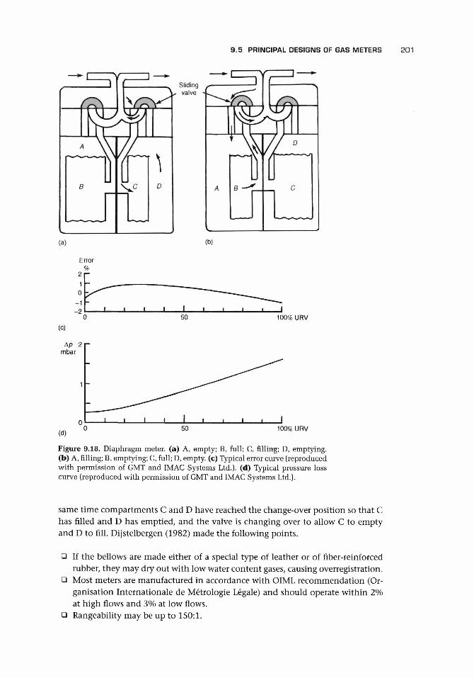
9.5 PRINCIPAL DESIGNS OF GAS METERS 201
Sliding* valve
(b)
Error
50 100% URV(c)
Ap 2 pmbar
(d)50 100% URV
Figure 9.18. Diaphragm meter, (a) A, empty; B, full; C, filling; D, emptying.(b) A, filling; B, emptying; C, full; D, empty, (c) Typical error curve (reproducedwith permission of GMT and IMAC Systems Ltd.). (d) Typical pressure losscurve (reproduced with permission of GMT and IMAC Systems Ltd.).
same time compartments C and D have reached the change-over position so that Chas filled and D has emptied, and the valve is changing over to allow C to emptyand D to fill. Dijstelbergen (1982) made the following points.
• If the bellows are made either of a special type of leather or of fiber-reinforcedrubber, they may dry out with low water content gases, causing overregistration.
• Most meters are manufactured in accordance with OIML recommendation (Or-ganisation Internationale de Metrologie Legale) and should operate within 2%at high flows and 3% at low flows.
• Rangeability may be up to 150:1.

202 POSITIVE DISPLACEMENT FLOWMETERS
The typical measurement uncertainty is ±1% [Figure 19.18(c)]. The maximumallowable inlet pressure on some designs is about 0.1 bar above atmospheric, butit may be up to 1 bar on other special versions. The coupling from the mechanicalmeter to the output may consist of a magnetic coupling to the display. Operatingtemperature range is typically -20 to +60°C. The meters operate to DIN 3374 andBS 4161. The pressure loss through the meter is about 1.5 mbar [Figure 19.18(d)].
9.5.3 ROTARY POSITIVE DISPLACEMENT GAS METER
The rotary positive displacement gas meter is, sometimes, referred to as a Rootsmeter, but this name, in a particular style, is the registered trademark of a particularmanufacturer's design (Dresser). Figure 9.19(a) shows a diagram of another design ofthis meter. Two rotors mesh and rotate within an oval body contour so that leakageis at a minimum between the rotors, but the gas is transferred at the outer point ofthe oval. In recent years they have performed to an increasingly high specificationand offer one of the best options for high precision gas flow measurement. Thereis a possible problem due to pulsating flow resulting from the use of these meters(Dijstelbergen 1982), and rapidly changing flow rates may damage them or down-grade their accuracy. The two rotors have a very small gap between (described byone manufacturer as less than a human hair), and the manufacture is to tight toler-ances on impellers and meter body. It is, therefore, necessary for the gas to be freeof particulate matter and for the meter to be mounted so that the tight tolerancesare not distorted. The gas flow can be distributed to give an even distribution overthe full length of the rotor entry.
Maximum flows are from 28 m3/h at 0.5 in. (13 mm) water gauge to 360 m3/h,with a pressure loss of 0.5 to 1 in. (13-25 mm) of water gauge. Figure 9.19(b) shows atypical performance characteristic with a performance well within 0.5% over a 10:1turndown. In fact, the claims are that 80:1 may be achievable. Temperature range isfrom -40 to 65°C.
Transmission can be through timing gears on the end of the shafts, with directcounter driven or with magnetic couplings.
The rotors may be hollow extruded aluminum with self-cleaning tips and a bodyof cast aluminum. The surfaces may be anodized.
(a)
% Error3
2
1
0
-2
-3
(b)
20 30 40 50 60 70 80 90 100 110 120%URV
Figure 9.19. Rotary positive displacement gas meter (reproduced with permission of Romet Ltd.and IMAC Systems Ltd.): (a) Diagram of meter; (b) Plot of the performance characteristic for themeter.

9.6 POSITIVE DISPLACEMENT METERS FOR MULTIPHASE FLOWS 203
The CVM meter is of similar design to Figure 9.3(b) with a main rotor that consistsof four vanes or moving walls that form metering compartments. The second rotoris a sealing rotor that returns the vanes to the inlet side of the meter. The secondrotor may be two- or three-lobed, and its rotation will be precisely linked to thatof the main rotor. According to Dijstelbergen (1982), it is suitable for high pressuremetering, does not cause pulsations in the flow, handles flows up to 1,200 m3/h, anda repeatability of 0.05% may be achievable.
9.6 POSITIVE DISPLACEMENT METERSFOR MULTIPHASE FLOWS
In a patent (1981), Arnold and Pitts proposed temperature and pressure sensingand a gamma-ray densitometer for sensing density inside a positive displacementflowmeter (Figure 9.20), but they gave no experimental data. However, the patentpresents an attractive device, which has the attribute of forcing the flow into aclosed volumetric space regardless of the flow components. A major disadvantage isthe possibility of solids causing it to seize up and block the line, requiring designsto have large clearances and consequent loss of precision.
An alternative approach has been taken by Gold et al. (1991) who used a he-lical rotor meter (Figure 9.21). In this design, two rotor sections are used in se-ries, and between them is a section where the condition of the multiphase flow ismeasured.
Gold et al. (1991) described their solution, which controls the flow being mea-sured and so avoids the problem of slip between phases. The helical rotors are alsoclaimed to be more resilient, with suitable bearings, to the rigors of multicomponentflow, reducing the possibility of damage due to transients. Between the two rotors,
Temperatureand pressure Radiation source andsensing sensor region
Radiationtransmissionregion
Slidingvanes
Figure 9.20. Diagram based on Arnold and Pitts' patent (1981) (reproduced fromBaker 1991a; with permission of the Council of the Institution of MechanicalEnigneers).
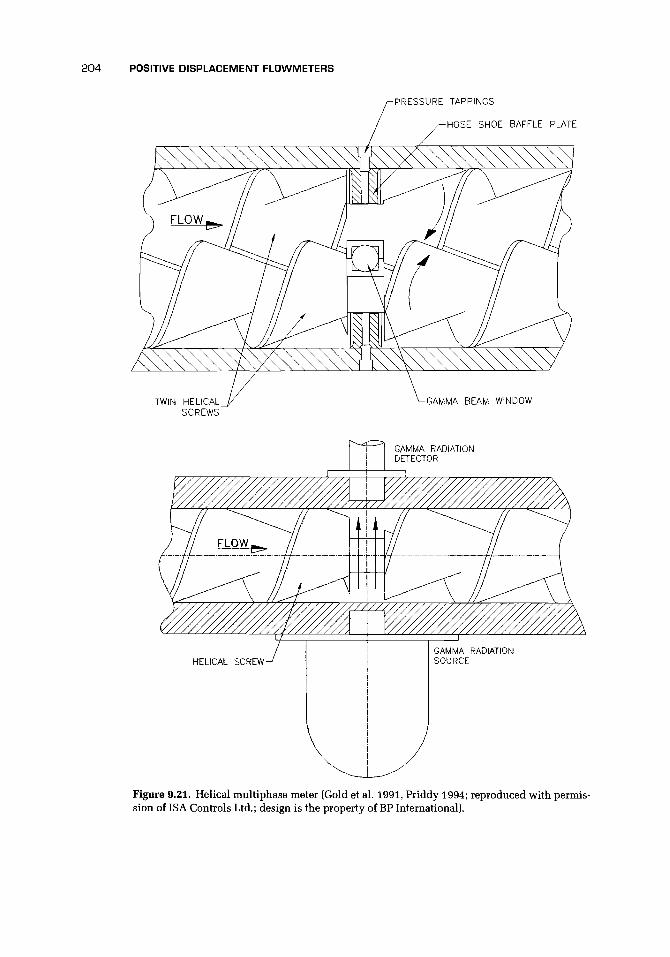
204 POSITIVE DISPLACEMENT FLOWMETERS
PRESSURE TAPPINGS
HOSE SHOE BAFFLE PLATE
TWIN HELICALSCREWS
GAMMA BEAM WINDOW
GAMMA RADIATIONDETECTOR
Figure 9.21. Helical multiphase meter (Gold et al. 1991, Priddy 1994; reproduced with permis-sion of ISA Controls Ltd.; design is the property of BP International).

9.8 APPLICATIONS, ADVANTAGES, AND DISADVANTAGES 205
t I
Figure 9.22. Meter using liquid plugs to measure low flows.
the density is measured. The preferred orientation is with flow vertically downward.The bearings are simple low friction journals but with thrust bearings that give longservice.
The meter was seen as suitable for both surface and subsea service and aimed at aspecification of ±5% rate for total flow and ±5% rate for oil flow rate with ±10% forboth gas and water. The field trial meters were designed for up to 20,000 barrels perday (130 m3/h) with at least 10:1 turndown and ±5% uncertainty. A nominal 4-in.(100-mm) bore meter was specified. The body had about 0.3-m outer diameter. Themeter length was 1.2 m, and with nucleonic densitometer it weighed about 450 kg.The scatter on test appears to be a maximum of about 20% in mid values of voidfraction. Priddy (1994) reported tests at Prudoe Bay, Alaska, which are extremelypromising in terms of the specific aims.
9.7 METER USING LIQUID PLUGS TO MEASURE LOW FLOWS
Figure 9.22 shows a diagrammatic representation of a meter that uses liquid plugsof a sealing fluid such as distilled water to measure the flow of gas. The plugs arecarried through the tube as shown, and the passage and velocity are sensed optically.Accuracy claims are ± 1 % at the optimum rate, and the range is 8-3,000 ml/h. Inthis device, dry gases pick up moisture. It is not clear how the size of plug, whichpresumably varies, is allowed for. It may be that the optics provide a compensation.
9.8 APPLICATIONS, ADVANTAGES, AND DISADVANTAGES
ApplicationsThe applications will vary to some extent for the various designs; in particular, theaccuracy and cost of the meters will make them more suitable for particular applica-tions. In general, they operate on clean or well-filtered fluids. The clearances are sofine that dirty or aggressive fluids may prevent operation and cause total blockage inthe line. For the same reason, the instruments must be correctly mounted to avoidmechanical distortion, which could affect the clearances.
In particular, for the sliding vane meter, one manufacturer claimed: blending,batching, dispensing, inventory control, custody transfer of oils, solvents, chemicals,paints, fats, and fertilizers.
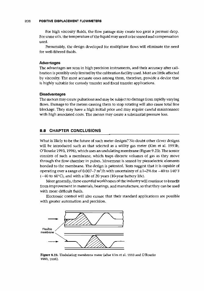
206 POSITIVE DISPLACEMENT FLOWMETERS
For high viscosity fluids, the flow passage may create too great a pressure drop.For some oils, the temperature of the liquid may need to be sensed and compensationused.
Presumably, the design developed for multiphase flows will eliminate the needfor well-filtered fluids.
AdvantagesThe advantages are seen in high precision instruments, and their accuracy after cali-bration is possibly only limited by the calibration facility used. Most are little affectedby viscosity. The most accurate ones among them, therefore, provide a device thatis highly suitable for custody transfer and fiscal transfer applications.
DisadvantagesThe meters may create pulsations and may be subject to damage from rapidly varyingflows. Damage to the meters causing them to stop rotating will also cause total lineblockage. They may have a high initial price and may require careful maintenancewith high associated costs. The meters may create a substantial pressure loss.
9.9 CHAPTER CONCLUSIONS
What is likely to be the future of such meter designs? No doubt other clever designswill be introduced such as that selected as a utility gas meter (Kim et al. 1993b,O'Rourke 1993,1996), which uses an undulating membrane (Figure 9.23). The sensorconsists of such a membrane, which traps discrete volumes of gas as they movethrough the flow chamber in pulses. Movement is sensed by piezoelectric elementsbonded to the membrane. The design is patented. Tests suggest that it is capable ofoperating over a range of 0.007-7 m3/h with uncertainty of ±1-2% for -40 to 140°F(-40 to 60°C), and with a life of 20 years (10-year battery life).
More generally, these essential workhorses of the industry will continue to benefitfrom improvement in materials, bearings, and manufacture, so that they can be usedwith more difficult fluids.
Electronic control will also ensure that their standard applications are possiblewith greater automation and precision.
Figure 9.23. Undulating membrane meter (after Kim et al. 1993 and O'Rourke1993, 1996).

9.A.1 FLOWMETER EQUATION 207
The successful use of positive displacement meters in such a hostile environmentas oil-well flows suggests that other difficult applications may be within range.
Total blockage of the line in the event of failure is, perhaps, the greatest disad-vantage, and ways of dealing with this through an automatically controlled bypass,in the event of blockage, may overcome this problem.
APPENDIX 9.A
Theory for a Sliding Vane Meter
The theory of the meter was set out by Hahn (1968). In his paper he considered themotion of the vanes and calculated the radial velocity and acceleration if the internalcontrolling cam gave a sinusoidal motion. He noted that the resultant forces betweenvane and wall contributed to the wear of the vanes. Avoidance of jerky motion andshock stresses is clearly important.
He also calculated the volumetric flow rate (cf. Baker and Morris 1985 whose workwas in ignorance of that due to Hahn). Hahn pointed out that the radial motion ofthe vanes results in a sinusoidal fluctuation superimposed on the volume versusrotation characteristic and that the amplitude of this fluctuation can be of order0.05-0.1% for various designs. This, in turn, would be shown in an irregularityof the rotation of the shaft of as much as 1.25%. However, in practice there willbe a balance between varying flow, pressure variation, and rotor velocity variation.Hahn also gave characteristics showing variation of within 0.2% over a range of 14:1(slight drop of 1.5-2% with increasing flow) and changes of +0.15% for a change inviscosity from 0.75 to 4 cP.
9.A.1 FLOWMETER EQUATION
The ideal behavior of the meter is given by the product of transferred volume, thenumber of volumes transferred per revolution, and the rotational speed. For the ac-tual behavior allowance has to be made for the leakage that takes place past the mov-ing rotors. The bulk volumetric flow for a meter of the sliding vane type is given by
qy = [n (r02 - rf) - 8] Nlax - Leakage flow (9.A.I)
where £ax is the axial length of the chamber. The flow in each gap (Figure 9.A.I) willbe governed by
z (9.A.2)dy
where [i is the fluid velocity at y in the gap, t is the clearance, pu and pa are theupstream and downstream pressures, L is the length of the clearance gap or, in thecase of the vanes, the thickness of the vanes, and /JL is the viscosity. This results in a

208 POSITIVE DISPLACEMENT FLOWMETERS
,1Figure 9.A.I. Geometry of leakage path between fixed and moving parts of themeter (after Baker and Morris 1985).
velocity distribution of
u = ^-i (t-Uy
and a volumetric flow through the gap of
1 (Ai - Pd)., Ut
(9.A.3)
(9.A.4)
where I is the axial length of the gap.If the rotor is stationary, this quantity becomes the slippage;
(9.A.5)
Ideally, the liquid in the gap would be carried at the same speed as the rotorblade:
(9.A.6)
(9.A.7)
(9.A.8)
From Equations (9.A.I) and (9.A.8) and assuming that the leakage can be taken asthe sum of leakage through clearances tj of length in the direction of leakage L;
and in the direction perpendicular to the leakage lj and with velocity of movingcomponent [/,-,
<?ideal = Uti
From Equations (9.A.4) and (9.A.6)
^leakage = ^ideal — <?v
SO
\ut i (Pu-Pd)^
(9.A.9)
An expression for the pressure drop across the vanes is obtained from the torquebalance on the rotor. The turning force due to (pu - pd) will act on a vane and willprecisely balance the frictional torques caused by bearings, vane clearance spaces,and readout mechanism:
(9. A. 10)
9.A.2 EXPANSION OF THE FLOWMETER DUE TO TEMPERATURE 209
where 7o is a constant torque and T\N/Nmax is a speed-dependent torque. Part of thetorque TiN/Nmax will be due to the clearance drag torque:
where r; is the radius from the rotational axis of the ;th clearance.
9.A.2 EXPANSION OF THE FLOWMETER DUE TO TEMPERATURE
If am is the coefficient of linear expansion of the metal, then a change in temperatureATm of the metal of the flowmeter will cause a change in length
so that
^=3amATm (9.A.12)
giving the fractional change in measured volume per revolution of the flowmeterrotor.
Differential ExpansionIf the expansion of the rotor differs from that of the casing due either to differenttemperatures or to different materials, then the clearances will be designed for thegreatest relative movement between these members. The change in the value of theclearance t will be
- = a m A T m - (9.A.13)
between uniform temperature conditions and conditions when the temperature ofthe internal rotor and the casing differ by A 7^. For the case where the temperaturesare the same but the coefficients of expansion differ, this becomes
At r~
(9.A.14)
Liquid Density ChangeThe change in the bulk flow due to expansion of the liquid will be
(9.A.15)
where at is the coefficient of volume expansion of the liquid.Because many liquids are bought and sold by volume, this change is of a different
significance from those given before. The volume passed by the meter may, therefore,be important. In some cases, the change in liquid density may be ignored.

210 POSITIVE DISPLACEMENT FLOW METERS
9.A.3 PRESSURE EFFECTS
Provided that the meter is supplied with an outer pressure vessel, there should be nonet pressure causing distortion of the inner meter. However, this is not invariablyso. The meter will then suffer from two distortions, hoop stress and axial stress. Forconvenience, we will consider these effects separately and ignore the effects of oneon the other.
Bulk Flow ErrorIf Ap is the difference between internal and external pressure and E is Young's mo-dulus of elasticity, then the change in the outer radius will be
IT-IT (9A16)
where £, is the thickness of the outer casing. The axial stress will cause an elongationof
where £ax is the axial length of the meter's measuring chamber. Together these lead(neglecting Poisson;s ratio effects) to an increase in measuring volume, which causesan error in the volumetric flow rate of
Leakage GapIn certain designs, the hoop stress will cause an increase in the clearance of
At = Arc = rjApt t ttoE v ;
whereas the axial stress will cause an increase in end clearance at each end ofAt A£ax ro4x Apt t
(9.A.20)
Clearly these calculations are simplifications of the actual expansion that will occur,but they allow some estimate of likely errors to be made.
9.A.4 METER ORIENTATION
Bearings at Each End of ShaftAssuming that the shaft behaves like a beam simply supported at each end and thatthe rotor weight is evenly distributed along the shaft, then the maximum deflectionat the point midway between the bearings will be given by
Deflection = SMgi\ (9.A.21)

9.A.5 ANALYSIS OF CALIBRATORS 211
where M is the mass of the rotor, g is acceleration due to gravity, and rs is shaftradius.
Bearing(s) at One End of Shaft OnlyAssuming that, in this case, the bearing(s) hold the shaft without deflecting, the shaftbending will be equivalent to a uniformly loaded encastre beam. The end deflectionof this, which will be the maximum value, is given by
Mai3
Deflection = y a* (9.A.22)
It is apparent that, other things being equal, the deflection of the end bearing shaftwill be nearly 10 times greater than the shaft with bearings at each end. This willrequire greater clearances and, consequently, allow greater leakages. To avoid thisproblem, it may be recommended that meters be mounted with shafts vertical.
9.A.5 ANALYSIS OF CALIBRATORS
The rotation of these meters gives the volumetric flow. If every rotation causes apulse, it is a simple matter with modern electronics to scale the pulse rate to giveany required calibration factor or combine the electrical output from a temperaturesensor to give a temperature compensation. However, in many applications, me-chanical calibration and temperature adjustment is required as a result of existinginstallation constraints, and three main methods have been used or are possible.
GearboxThe gearbox with interchangeable gears will not be discussed in this section. Thedrawback of the gearbox is clearly the limited adjustment possible. We are concernedwith two calibrators, which may introduce special features into the meter perfor-mance.
Epicyclic SystemA schematic diagram of this system is given in Figure 9.10. The drive from theflowmeter shaft enters with rotation 2VIN. The drive then divides. The main driveis via gears tt\, n2, n3, and so to the epicyclic unit. The other is via the disk andadjustable friction wheel to ns,n7. The recombined drives leave the epicyclic unitvia n6 with rotation A/OUT- The integrity of the unit depends heavily on the wheel anddisk contact. There must be no slip between these components, but they must alsonot wear and must be adjustable (r the radius of frictional contact being changed bythe adjustment).
The ratio of NOUT/MN is given by
NOUT ^ L ffcWs 1 rnn3nsNIM Rn7 [ n4n6\ n2n4n6
where R is the radius of the friction wheel.

212 POSITIVE DISPLACEMENT FLOWMETERS
Putting typical values of the numbers of teeth (ri) into Equation (9.A.23)
n2 = rii
n4 =
n6 =
1520n5
~15~n7 = Sn8
then
NQUT
If JR = 10 mm and we let r = 10 mm,
^ ^ = -0.508
Ifr = 11 mm,
1ST = - ° - 5 0 3
or a change in calibration of 1%.We may also write down the modified version of Equation (9.A.23), assuming
that a small amount of slip occurs between disk and wheel equivalent to a rotationNs in NIN. Then
K™ = LnA d _ Hi!!*] (i-**L\- ^ ^ (9.A.24)NIN R n7 \ n4n6j \ NiN) n2 n4 n6
In this case, a relation between the torque in TiN and the torque out TOm, the frictionforce between wheel and disk F, is given by
(9.A.25)
At the start of rotation if NOUT were zero and NiN were nonzero, then
NIN
and
n2 n4 n6= 1-
R n7 V n4 n6
Using the values given earlier,
—5- = -9.2
TlN = -9.2 rF

9.A.6 APPLICATION OF EQUATIONS TO A TYPICAL METER 213
If slip does not occur, then
NOUT rj,iiN = —j^— -four
NIN= -0.508 TOUT
With these relationships and the coefficient of friction, the required contact forcebetween wheel and disk can be estimated from a knowledge of the torque requiredto operate the counter unit.
Clutch SystemThe clutch (or cam) system consists of three concentric disks and rings (Figure 9.11).The central ring is driven by the input shaft and carries a series of clutches that lockon the center disk and the outer ring, causing them to rotate at least as fast as thecentral ring. An arm rotates on a separate shaft, which is not concentric with thatof the disk and rings. In this arm are two sliders, one fixed to, and rotating with, thecenter disk and the other fixed to, and rotating with, the outer ring. Because of theeccentricity of the arm shaft, the center disk and the outer ring are forced to rotate atdifferent speeds. The difference in speeds can be adjusted by manually altering theamount of eccentricity. Thus, the speed at which the output shaft revolves relativeto the input shaft is adjusted to achieve compensation for use of the measuringelement under a particular set of operating conditions. It can be shown that if O isthe angular position of the arm and 0c and 0o are, respectively, the angular positionsof the center disk and outer ring [Figure 9.A.2(a)]
fp ) (9.A.26)
and
* = 0o + tan"1 ( A f e \ ) - * (9.A.27)y^ + Acos^/
where A is the distance between the centers of rotation of the arm and the disks.These are plotted in Figure 9.A.2(b), and it can be seen that at <J> = 0, n, and 2nf
the angular positions differ by n. The angular velocities will be equal when, for agiven value of $, the slopes of 6C and 00 are equal.
In Figure 9.A.2(c), the relationship between output rotational speed No and inputrotational position 0x (which for constant flow rate is proportional to time) is plotted.It is important to note the nonuniform rotation of the output and the mean valuein relation to actual rotational speed at various points in the cycle.
9.A.6 APPLICATION OF EQUATIONS TO A TYPICAL METER
Using the meter with dimensions shown in Figure 9.13 and Equation (9.A.9), weobtain for the main coefficients, assuming a total leakage length of 325 mm,
qv = 0.00918N-0.0000156N (leakage)
+0.034 x 10~10— (leakage due to pressure change)

214 POSITIVE DISPLACEMENT FLOWMETERS
Figure 9.A.2. Clutch calibration ad-justment system (reproduced fromBaker and Morris 1985; with per-mission of the Institute of Measure-ment and Control): (a) Geometry;(b) Rotational position of centerdisk and outer ring against arm po-sition; (c) Rotational output speedas a function of input rotational po-sition.
No
/11I
! /1/.
^ \ No
\1I1
i 0 = T
/, !/ , .
2n 3Tt
22T1
(c)
Taking
Ap = 20000 N/m2
[i = 0.1 Poise
qv = 0.00916N + 0.677 10~6 m3/s
The sensitivity to t and Ap is given by
qv = 0.00918N - 0.156tN + 3
Taking the datum values of t = 0.1 mm, Ap = 0.2 x 10⁵ N/m2 and /x = 0.1 poise, theeffect of changes of ±0.5Ap//x for N = 1 revolutions per second and t = 0.2 mm isabout ±0.05% (Baker and Morris 1995).
CHAPTER 1O
Turbine and Related Flowmeters
10.1 INTRODUCTION
10.1.1 BACKGROUNDSpirals, screws, and windmills have a long history of use for speed measurement.Robert Hook proposed a small windmill in 1681 for measuring air velocity and laterone for use as a ship's log (distance meter). A Captain Phipps, in 1773, created aship's log, using the principle that a spiral, in turning, moves through the lengthof one turn of the spiral. Many centuries earlier, it appears that a Roman architect,Vitruvius, suggested a more basic form of this device.
In 1870 Reinhard Woltmann developed a multibladed fan to measure river flows(Medlock 1986). The device was a forerunner of the long helical screw-type meterstill called after him and used widely for pipe flows in the water industry. The firstmodern meters, of the type with which we are mainly concerned, were developed inthe United States in 1938 (Watson and Furness 1977; cf. Furness 1982). These wereattractive for fuel flow measurement in airborne applications. They consisted of ahelically bladed rotor and simple bearings. Improved sleeve bearings were developedfor longer life with hardened thrust balls or endstones to withstand the axial load.An alternative, developed over several years and patented by Potter (1961), was toprofile the hub of the rotor so that the pressure balance across the rotor, rather thanthe thrust on the bearings, held it against the axial drag forces. This allowed therotor to run on a single journal bearing.
10.1.2 QUALITATIVE DESCRIPTION OF OPERATIONThe turbine consists of a bladed rotor that turns due to the flow in the pipe. Inmost of the designs to be discussed, the rotor is designed to create the minimumdisturbance as the oncoming flow passes around it. Ideally, it cuts perfectly throughthe fluid in a helix so that every revolution of the helix represents one completeaxial length of the screw, and hence a calculable volume of the fluid. In practice,there are drag forces, which slightly retard the rotation. These result from frictionaldrag on the blades, the hub, the faces of the rotor, and the tip of the blades; bearingdrag, also a frictional effect; and drag due to the means by which the rotation ismeasured, which is usually a magnetic drag. These drag forces affect the otherwiseideal relationship of constant fluid volume for each rotor revolution and lead tononlinearity.
215

216 TURBINE AND RELATED FLOWMETERS
The rotor has to be held in the stream, and so supports are invariably necessaryto position the bearings centrally in the pipe. Virtue is made of necessity, and thesesupports are used to provide some flow straightening, since the turbine meter is of atype particularly susceptible to swirl. The oncoming fluid will therefore need to flowover the upstream support, and the naturally occurring profile, where the velocity ofthe fluid is lower at the pipe wall than at the center of the pipe, will be redistributedinto the annular passage past the blades, and, perhaps most importantly, there will bea reduction in any swirl component due both to conservation of angular momentumduring the redistribution and to the straightening effect of the supports. The velocityin this passage will vary a small amount with radial position, and a well-designedturbine rotor will generally have helical blades to match the axial and tangentialvelocity of the rotor at each radial position.
The main variants from this description are the Pelton and vane or paddle wheeldesigns. In the former, a tangential jet of fluid hits the buckets or blades of the wheeland causes them to rotate. This design has two alternative virtues: it can be madeas a simple insertion probe to obtain an estimate of the flow rate, or it can be usedin very small flows to register where other designs fail. Other designs using largerpaddle wheels and angled propellers are also available (cf. Baker 1991b, 1993).
10.1 .3 BASIC THEORY
Many turbine meters use flat section blades. Ideally these will cut smoothly throughthe flow in a perfect helix. Using this basic concept, the value of Vz can be obtainedfrom the frequency of blade passing f (Figure 10.1). Thus,
= W/t<m/3
and
f=N tan
(10.1)
(10.2)
where Vz is the axial velocity of the flow approaching the blades, W is the bladevelocity, f5 is the blade angle, N is the number of blades, and r is the radius of theblades at the measurement point.
Equation (10.2) can be used to obtain
f=Kqv (10.3)
Figure 10.1. Relationship between velocities and angles for ideal flow overblades.

10.1 INTRODUCTION 217
Profile A Profile B
<t
Figure 10.2. Velocity profiles at inlet to, and in the annulus of, a turbine meter.
which provides the basis for the constant, which in various units and dimensionsis known as meter registration, meter constant, meter coefficient, calibration factor,etc., and is measured in pulses per unit volume or radians per unit volume. We shallcall this the K factor, in (pulses per cubic meter), as in Chapter 1.
Tan (1973; cf. Fakouhi 1977) gives an equation of the form
-*- = a0 +qv qy q*
(10.4)
where the second term is affected by the viscosity and leakage, and the third termis affected by the mechanical and aerodynamic drag. Adjusting these two terms hasbeen found to affect the familiar hump in the turbine characteristic (cf. Newcombeet al. 1972 who gave an equivalent equation for gas meters).
However the theory is not, unfortunately, as simple as this because the blades donot cut the fluid perfectly, and the value of r and /3 must change to accommodatethe profile across the pipe.
Suppose that we consider the variation of blade angle for a uniform profile A(Figure 10.2), then it can be seen that, with no variation in axial velocity across theannulus, the correct blade angles will be given by
tan/3/r = constant (10.5)
If the midspan blade angle is 41° as in Xu's papers (1992a, 1992b) then thevalues at hub and tip will be 30° and 49° as in Xu's meter, suggesting that this wasthe method applied in the design which he used. If, however, profile B existed, thenthe flow will not meet the blades at the correct angle, and the designer may adjustthe blade twist to allow for this. The reader is also referred to Hochreiter's (1958)paper where he allows for blade obstruction.
It thus becomes apparent why the flowmeter will be susceptible to incorrectinstallation, since this will cause a flow profile that results in the wrong incidenceangle for some parts of the annulus. It also suggests why a turbine wheel, which isoptimized for flow profile range, will give a better performance than one with, say,constant angle blades. To develop a fuller theory, it is necessary to take account ofthe lift and drag on the blades, bearings, etc. Figure 10.3 sets out the main anglesand forces for a cascade of blades. The analysis is given in Appendix 10.A.1.
Tsukamoto and Hutton (1985) predicted the complete characteristic of a turbinemeter with reasonable accuracy allowing for viscosity, inlet flow profile, and metergeometry. Blows (1981) developed a model of a turbine flowmeter, which allowedthe effects of viscosity and tip clearance to be examined.

218 TURBINE AND RELATED FLOW METERS
Figure 10.3. Cascade angles, dimensions, and forces.
The equation for the driving torque [Equation (10.A.1)], given by Tsukamotoand Hutton (1985) (Figure 10.4) and equivalent to the equation used by Blows(1981), is equated to the drag torque. Tsukamoto and Hutton (1985) gave fourcomponents of the drag torque:
Tb, the bearing drag;Tw, t he h u b disk friction drag;Tt, t he blade t ip clearance drag; andTh, t he h u b fluid drag.
Blows (1981) discussed pickup torque and thrust pad drag torque bu t dismissedthe former as difficult to calculate and likely to be significant only in small meters.He suggested tha t t he thrust pad force migh t vary, no t only in sign, bu t by a factorof 100; hence , because effects of this significance are no t observed, it could also
be ignored. The consensus appears to betha t the dependence of all drag forces o nspeed, apart from aerodynamic drag on theblades and the h u b fluid drag, is a power lesst h a n two and therefore of decreasing signif-icance wi th increasing speed.
Tsukamoto and Hut ton 's (1985) resultswere impressive, giving a characteristicshowing the h u m p and the effect of theblade boundary layer t ransi t ion at differ-ent blade posit ions at different radii, andthe linear range w h e n the boundary layeris turbulent (Figure 10.5). This h u m p has
, . r , been at tr ibuted to skin friction and toFigure 10.4. General view of a turbine rotor andtorques on the rotor (based on Tsukamoto and Hutton unsteady wake flow caused by straight-1985; with the authors' permission). eners. Tsukamoto and Hutton (1985) also

10.1 INTRODUCTION 219
Turbulent
Transition / —
Laminar . 1
3.4
3.2
Power Law Upstream Profile
1*10~6m2/s
Parabolic Upstream ProfileMeasured by Fakouhi (1977)
o v »• 21A 47a 170
, , , , • • . , ! . . . . . . ..I I
10° 10* 10°Re
Figure 10.5. Comparison between calculated and measured meter performance. Relevant di-mensions: r0 = 18.288 mm, rt = 18.008 mm, rh = 9.703 mm, B = 14.224 mm, tB = 1-245 mm,L = 95.280 mm, N = 6,fj = 2.477 mm, o, v = 1 x 10"6 m2/s, • . v = 21 x 10~6 m2/s,A, v = 47 x 10~6 m2/s, D, v = 170 x 10~6 m2/s (based on Tsukamoto and Hutton 1985; withthe authors' permission).
obtained good qualitative agreement for the effect of change from uniform to fullydeveloped turbulent inlet profile and for tip clearance between Tan (1973), Jepsonand Bean (1969), and their own theory.
Thompson and Grey (1970) derived expressions for rotor hub fluid drag andblade tip clearance drag and introduced the bearing drag and the pickup drag. Usingcalculated annulus flow profiles, they demonstrated that, even with helical blades,the profile results in a variation of angle of attack for a 50-mm meter of +7° to -8°and because the actual incidence angle will be greater than the angle of attack, it ispossible that blade stall may be occurring. The effect of this on the driving torqueis best shown in a plot of torque against radius. It is also useful to note that changeof fluid for the same velocity results in a change in Reynolds number and hence inprofile, although the effect on angle of attack is comparatively small. The annulusprofiles and the blade driving torque are shown in Figures 10.6 and 10.7.
Jepson and Bean (1969) in their earlier work essentially reproduced Equation(10.A.1) with a slightly different constant. In their analysis, they made three simpli-fying assumptions.
a. They assumed that the exit angle was the blade angle and for helical blades wouldbe given by [cf. Equation (10.5)]
= tan"1 2nr\ (10.6)
where Kh is a constant.

220 TURBINE AND RELATED FLOWMETERS
10
IITY,
m/s
I 91—JJ
? 6LJU-7
TUR
Bir
CO
n
-
-
—
-
!
// ^ ^ v WATER
II *%II OIL V/
I 1 ! 1 110 15
RADIUS, mm
20 25
Figure 10.6. Turbine inlet velocity profiles for water and oil (Thompson andGrey 1970; reproduced with permission from ASME).
b. They assumed that the retarding torque caused by bearing friction was negligiblecompared with the aerodynamic forces, and they justified this on the groundsthat it is constant. They pointed out that the assumption was only valid forcommercial meters with low resisting torques.
c. They did not consider retarding torques apart from bearing friction and bladeaerodynamic drag.
They used this simple approach to examine the effect of flow profile and, know-ing the profile downstream of a cone exit, to calculate meter error with distancefrom the cone exit.
Hutton has made the point that a basic difficulty in applying blade theory to tur-bine meters is that their blades are not very like flat plates because the parallelogram
DCQ
LU -22 —
5=> -44 —ODCOS -66 -
-88
Figure 10.7. Driving torque per unit blade length for water and oil (Thompsonand Grey 1970; reproduced with permission from ASME).
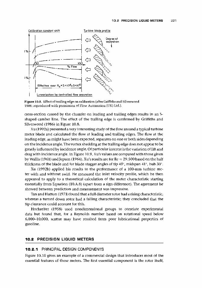
10 .2 PRECISION LIQUID METERS 221
Calibration constant shift Turbine blade profile
Degree ofseparation
I
Linearization by controlled flow separation
Figure 10.8. Effect of trailing edge on calibration (after Griffiths and Silverwood1986; reproduced with permission of Flow Automation (UK) Ltd.).
cross-section caused by the chamfer on leading and trailing edges results in an S-shaped camber line. The effect of the trailing edge is confirmed by Griffiths andSilverwood (1986) in Figure 10.8.
Xu (1992a) presented a very interesting study of the flow around a typical turbinemeter blade and calculated the flow at leading and trailing edges. The flow at theleading edge, as might have been expected, separates on one or both sides dependingon the incidence angle. The vortex shedding at the trailing edge does not appear to begreatly influenced by incidence angle. Of particular interest is the variation of lift anddrag with incidence angle. In Figure 10.9, Xu;s values are compared with those givenby Wallis (1961) andjepson (1964). Xu's results are for Re = 29,500 based on the halfthickness of the blade and for blade stagger angles of tip 49°, midspan 41°, hub 30°.
Xu (1992b) applied his results to the performance of a 100-mm turbine me-ter with and without swirl. He measured the inlet velocity profile, which he thenappeared to apply to a theoretical calculation of the meter characteristic startingessentially from Equation (10.A.8) (apart from a sign difference). The agreement heshowed between prediction and measurement was impressive.
Tan and Hutton (1971) found that a full diameter rotor had a rising characteristic,whereas a turned down rotor had a falling characteristic; they concluded that thetip clearance could account for this.
Hochreiter (1958) used nondimensional groups to correlate experimentaldata but found that, for a Reynolds number based on rotational speed below6,000-10,000, scatter may have resulted from poor lubricational properties ofgasoline.
10.2 PRECISION LIQUID METERS
10.2 .1 PRINCIPAL DESIGN COMPONENTS
Figure 10.10 gives an example of a commercial design that introduces most of theessential features of these meters. The first essential component is the rotor itself,

222 TURBINE AND RELATED FLOWMETERS
1 . 0 -i
0.8 -
0.6 --
0.4 --
0.2 "-
Tip section(Xu)
0.2 •
0.4
0.6
0.8
Flat plate(reproducedby Wallis)
Blade elementat mid radius(Jepson)
20
Figure 10.9. Comparison of lift coefficient as given by various authors (Wallis1961, Jepson 1967, Xu 1992a).
which is like a small turbine. This is formed either from straight or twisted (helical)blades. For good design, it is suggested that the hub radius be approximately half thetip radius; the blades, when viewed axially, just block the cross-section of the pipe;and the axial length of the blades be approximately equal to the blade span, whichis the length of the blade from hub to tip.
It is important to remember that unlike the power turbine, the meter aims tocut through the fluid without disturbing the flow. This clearly is an impossible ideal;nevertheless, the power extracted from the fluid is very small, and the incidenceof the flow onto the blades is consequently also very small. The reason for thepopularity of helically twisted blades is that the relative angle of approach of thefluid onto the blades varies with radius. Consequently, flat plate blades will not allowa constant angle of attack and will lead to unnecessarily large incidence angles, bothpositive and negative, and thus will impart unnecessary flow disturbance and drag.
The rotor is usually machined from solid, and the flat plate blades often haveleading and trailing edges that are milled in a constant end plane. The cross-sectionof the blade at a constant radius will therefore be essentially a parallelogram. Sharpedges should be avoided because they may cause cavitation. Griffiths and Silverwood(1986) describe how small changes in the shape of the trailing edges can cause achange of the blades' aerodynamic drag and consequently of the meter calibration(Figure 10.8).

10.2 PRECISION LIQUID METERS 223
Figure 10.10. Precision commercial turbine flowmeter design for liquids for100—500 mm diameter (1, body; 2, rotor; 3, support nut; 4, support plate; 5,support tube; 6, support vane; 7, lock tab; 8, end support assembly; 9, flange;10, pickup assembly; 11, pickup stub) [reproduced with permission of FlowAutomation (UK) Ltd.].
The hangers or support vanes that position the bearings centrally in the pipe arecommonly used as flow straighteners to reduce swirl. Their shape varies considerably.In Figure 10.10, they are flat plates, and in another design, they are parallel tubes. Therotation of the rotor is sensed by a pickup, which most commonly senses a changein the magnetic material permeability in its vicinity as a blade passes (magneticreluctance change). Alternatives to this are to use the eddy current effect or dynamoeffect as a blade passes through the magnetic field of the sensor (magnetic inductive)or to use a modulated high frequency signal (modulated carrier or radiofrequency).The capacitance effect can also be used to sense the proximity of a passing blade tothe sensor head. Optical fibers have been tried, but if the optical path passes throughthe fluid, there is a danger of the windows becoming fouled. For increased integrity,some meters have two sensors spaced at about 120°, the pulse trains from both aresensed, and the phase angle is constantly checked.
In small meters, the internals are held in position by circlips, the removal ofwhich allows the internals to be withdrawn. In other designs and larger sizes, thebearing assemblies may be removed from the body by releasing a taper locking nut.
10.2 .2 BEARING DESIGN MATERIALSMinkin et al. (1966) attributed calibration unpredictability to bearing variation as amajor factor.
Clean LiquidsOpen ball bearings of stainless steel or other compatible material are suitable forliquids with lubricating properties in the temperature range -50 to 250°C, but a

224 TURBINE AND RELATED FLOWMETERS
filter with a mesh size small enough to prevent solid particle ingress into the bearingsshould be used.
Liquids in GeneralTungsten carbide or high chrome/high cobalt journal bearings possibly with carbidepinions and a stellite sleeve are suitable in the range —50 to 400°C unlubricated.The bearings are lubricated by the metered fluid and made up of tungsten carbidewith a hardness of Rockwell C-94 and a surface smoothness of 0.05 /xm. Tungstencarbide with cobalt bonding is most common, but the cobalt is leached out by acidicsolutions used for cleaning. Stellite may then be used as a less durable alternativefor more corrosive fluids. A more recent alternative is nickel-bonded carbide busheswith titanium carbide shafts. An alternative design uses rotor pins of hard metal insapphire bearings with thrust plate and rings made with curved contact surfaces forline contact. Polytetrafluoroethylene (PTFE) is used in some applications. Ceramicbearings (e.g., A12O3), may also be an option.
One manufacturer has used a ball-and-sleeve design. The shaft was tipped withan ellipsoid and ran in a ceramic sleeve so that line contact was achieved. Typi-cal bearing life was claimed as 12-24 months when used with 50-75% duty cy-cle in clean particulate-free gasoline. For ball race bearings correctly lubricated, alife of 4,000-6,000 hours was claimed, and for journal bearings 20,000 hours ormore was claimed, depending upon the properties of the measured fluid and rate offlow.
For some larger sizes (above about 80 mm) only an upstream bearing is used; itconsists of a tungsten carbide (or other suitable materials) bush and shaft. Specialbearings are available for cryogenic applications (cf. Rivetti et al. 1987). Hydrostaticbearings may be suitable for dirty fluids. House and Johnson (1986) applied hydro-static bearings and obtained a remarkable performance (turndown ratio for waterof 1,000:1) and suitability for dirty fluids. Wemyss and Wemyss (1975) describedthe development of the Hoverflo bearingless meter. Some manufacturers provideapplication charts.
Ball bearings have been found satisfactory for cryogenic applications in rockettesting because of their ability to tolerate overspeed and operation with gas. However,journal bearings, although less linear, may be more repeatable.
10.2.3 STRAINERSTypical values for strainers are given by manufacturers with maximum allowableparticulate sizes (Table 10.1).
10.2.4 MATERIALSBecause the signal is usually obtained from magnetic sensing, it is common to makethe tube of austenitic stainless steel to allow the magnetic field to penetrate. How-ever, carbon steel is used for flanges and sometimes also for the bodies; in this in-stance, provision is made for the pickup assembly to function despite the magneticbody.
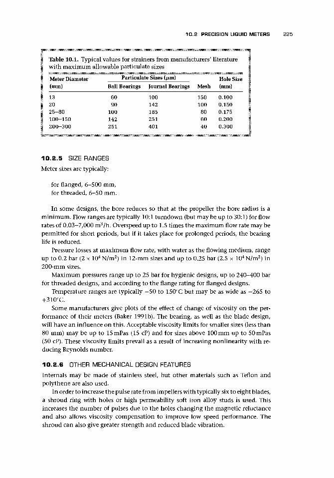
10.2 PRECISION LIQUID METERS 225
Table 10.1. Typical values for strainers from manufacturers' literaturewith maximum allowable particulate sizes
Meter Diameter(mm)
132025-80100-150200-300
rariicuiaBall Bearings
6090
100142251
ie sizes t/xmjJournal Bearings
100142185251401
Mesh
150100
806040
Hole Size(mm)
0.1000.1500.1750.2000.300
10.2.5 SIZE RANGESMeter sizes are typically:
for flanged, 6-500 mm,for threaded, 6-50 mm.
In some designs, the bore reduces so that at the propeller the bore radius is aminimum. Flow ranges are typically 10:1 turndown (but may be up to 30:1) for flowrates of 0.03-7,000 m3/h. Overspeed up to 1.5 times the maximum flow rate may bepermitted for short periods, but if it takes place for prolonged periods, the bearinglife is reduced.
Pressure losses at maximum flow rate, with water as the flowing medium, rangeup to 0.2 bar (2 x 10⁴ N/m2) in 12-mm sizes and up to 0.25 bar (2.5 x 10⁴ N/m2) in200-mm sizes.
Maximum pressures range up to 25 bar for hygienic designs, up to 240-400 barfor threaded designs, and according to the flange rating for flanged designs.
Temperature ranges are typically -50 to 150°C but may be as wide as -265 to+310°C.
Some manufacturers give plots of the effect of change of viscosity on the per-formance of their meters (Baker 1991b). The bearing, as well as the blade design,will have an influence on this. Acceptable viscosity limits for smaller sizes (less than80 mm) may be up to 15mPas (15 cP) and for sizes above 100 mm up to 50mPas(50 cP). These viscosity limits prevail as a result of increasing nonlinearity with re-ducing Reynolds number.
10.2.6 OTHER MECHANICAL DESIGN FEATURES
Internals may be made of stainless steel, but other materials such as Teflon andpolythene are also used.
In order to increase the pulse rate from impellers with typically six to eight blades,a shroud ring with holes or high permeability soft iron alloy studs is used. Thisincreases the number of pulses due to the holes changing the magnetic reluctanceand also allows viscosity compensation to improve low speed performance. Theshroud can also give greater strength and reduced blade vibration.

226 TURBINE AND RELATED FLOWMETERS
In some small designs of turbine meter, the blades have a T shape so that at thetip they are longer (longer chord) than at the hub. One reason given for this is toimprove insensitivity to viscosity change, which may result from a greater drivingtorque achieved by increasing the blade lift at the maximum radius. It may alsoflatten the characteristic hump at low speed. I am not aware of published data toconfirm these tendencies.
Some designs can be used bidirectionally, but, of course, they require calibrationin each direction.
Response time constants measured with water or with a liquid of similar densityrange from 0.005 to 0.05 s for a 50% flow rate change or up to 0.17 s to reach 63%of a step change final value.
After use with corrosive fluids, the meter should be cleaned with solvents. How-ever, maximum rotational speeds should be carefully observed.
10.2.7 CAVITATI0NCavitation is caused when the local pressure drops below the vapor pressure of theliquid and results in a two-phase flow of increased volume and, therefore, causesoverreading. Figure 10.11 demonstrates this effect where the vapor pressure of thehydrocarbon is less than 0.007 bar. It may also cause damage to the internals. Asimple rule is that the pressure downstream of the meter should be at least 1 barabove atmospheric pressure. More generally, the rule given is that the back pressureshould be at least twice the pressure drop across the meter plus the absolute vaporpressure times 1.25. This recognizes that, in addition to the pressure loss through themeter at rated flow of between 0.3 and 0.7 bar and the pressure needed to acceleratethe flow past the turbine wheel of 0.3-1.0 bar, there is also the minimum pressurelevel to prevent cavitation.
Bucknell (1963), from his work on liquid oxygen and hydrogen, suggested thata minimum safe margin for most meters was a back pressure of four times the meterpermanent pressure loss above the vapor pressure.
1.04
S 1-02
O
u 1.00
^ 0 .99
\\x
x O 125% rated flow\ • Rated flow\
J I I1 1.5 2 2.5
Meter outlet pressure (bar)
Figure 10.11. A typical example of cavitation effects on calibration factor(Shafer 1962; reproduced with permission from ASME).

10.2 PRECISION LIQUID METERS 227
10.2 .8 SENSOR DESIGN AND PERFORMANCE
A direct mechanical drive to register may be used in large meters. However mostcommonly, to obtain rotor speed, blade passing is sensed by the change in the mag-netic field around the sensor. The terms given to the various methods suffer fromsome variation, and the following are suggested for consistency (Olsen 1974):
a. Inductive: Magnets are embedded in the hub or blades, and a pickup coil with asoft iron pole piece senses their passage;
b. Variable reluctance: A permanent magnet with pickup coil is positioned in thebody of the flowmeter near the propeller/rotor, which senses the variation of theflux due to the passage of each blade or shroud ring stud of highly permeablemagnetic rotor material;
c. Radiofrequency (RF): An oscillator applies a high frequency carrier signal to thecoil in the pickup assembly, and the passing of the rotor blades modulates thecarrier. At very high frequencies of signal transmission, the skin effect is suchthat the electromagnetic field is essentially reflected by the passing blades withnegligible drag effect on the wheel.
d. Photoelectric: A light beam is interrupted by the passage of the blades. Opticalfiber methods, which are intrinsically safe, may also be used where the lightreflects off the blade tips. The problem with this method is that the windowstend to become fouled, and so light transmission through the liquid is not tobe recommended in many applications. Place and Maurer (1986) proposed anoptical system that overcame this problem where the blade passage rocked amagnetic element and the rocking was sensed optically;
e. Magnetic reed switch: Contacts are opened and closed by magnets in the rotor orsome rotating part of the meter.
The resulting signal must be amplified with care and shielded from extraneous noisedue to voltage sources or magnetic fields because spurious pulses can introduce sig-nificant errors.
Vibration may also cause microphonic effects. Screened cable should be used, andthe distance from the flowmeter to the preamplifier should be as short as possibleand typically not greater than 2 m.
Typically the pulse is amplified from about 15 mV root-mean-square (RMS) to 8V amplitude (increases with flow rate) and is of 0.5- to 20-ms duration. The pulse rateranges from 50 Hz to 3 kHz, and impedance from 300 to 1,500 ohms. A maximumtransmission cable length has been given as 1,000 m by one manufacturer. The signalis then applied to a signal converter, an electronic gearbox, to convert pulse rate intocubic meters per hour and total into cubic meters. A high pulse density is desirablewhere a meter is to be calibrated against a volumetric standard such as a prover loopwhere generally it is recommended that 10,000 pulses or more should be collectedper unit reference volume. Eide (1991) described a 12-in. Brooks Compact Proverand a 3-in. Brooks turbine meter modified to give 27,000 pulses/m3, which wereused to calibrate pipe provers. The uncertainty of the water draw was better than±0.003%, and the master meter's uncertainty was 0.02%.
Ball (1977) demonstrated that below about 1/3 FSD, the drag due to a magneticpickup could cause differences compared with an RF pickup and at 1/6 FSD couldindicate an error of 4% rising further with decreasing speed.

228 TURBINE AND RELATED FLOWMETERS
TypicalPerformanceCurves ±0.12% reading ovei
{restricted flow range±0.25% of reading overoperating flow range
Figure 10.12. Characteristic for a precision liquid meter after KDG Instruments(reproduced with permission).
10.2 .9 CHARACTERISTICSThe typical characteristic of the precision turbine meter is shown in Figure 10.12.There are four regions to note:
i. the highest accuracy region;ii. an extended range that should be used only briefly and with care to avoid excess
bearing wear;iii. the normal range of operation that includes both the high accuracy region and
also a lower flow region which is often shown as having a "hump"; andiv. a low flow region where drag forces are dominant and where the performance of
the meter is less reliable.
Most of these regions and their causes are obvious. The one that is often puz-zling is the hump region in (iii). Tsukamoto and Hutton (1985) have confirmedtheoretically that a hump in the characteristic can be caused by movement of thepoint of transition of the blade boundary layer near the leading edge of the bladesfrom turbulent in the high accuracy region to laminar. Griffiths and Silverwood(1986), as indicated earlier, have suggested that changing the profile of the bladetrailing edge by filing off the corner leads to a removal of the hump and an in-crease of speed of rotation of over 1% due, presumably, to changes in the point ofseparation and reduction of drag (Figure 10.8).
Pressure loss arises largely from the pressure reduction at the rotor and bearingsupports and the failure to recover fully the total pressure downstream for an arearatio m = A\/A2l which will give a maximum pressure loss of
For pressure change due to area change only (neglecting friction), the loss factorK = (m2 - 1), and for values of m = | , p = 103 kg/m3 and Vx = 10 m/s this gives apressure change of 0.39 bar (3.9 x 10⁴ N/m2). Experimental values of K range from 0.4to 0.9 depending on the geometric details of the meter. For K = 0.5, p = 103 kg/m3
and V\ = 10 m/s, the pressure loss is 0.25 bar.
10.2.10 ACCURACYTypical values of measurement uncertainty given by manufacturers are ±0.12-0.25%for the high accuracy range and ±0.25-0.5% for the lower part of the normal range.

10.2 PRECISION LIQUID METERS 229
This is sometimes given as a linearity. The meters are capable of calibration to achievethese values and possibly slightly better than ±0.1 to 0.5% over a turndown ratioof 6:1 at least and up to 18:1 for thrust-compensated designs. With achievable un-certainty of ±0.15%, they can meet the requirements of oil pipeline and custodytransfer applications.
Repeatability is typically given as ±0.05% for meters of less than or equal to50 mm and ±0.02% for meters of greater than or equal to 75 mm. Such precisionvalues do not take into account bias errors often present in calibration equipment.Mattingly et al. (1977) obtained day-to-day laboratory repeatability of ±0.07-0.12%.Shafer (1962) made the important point that before calibration the meter needsto be soaked in the calibration fluid and run for some time beforehand. He ob-tained impressive performances of 0.1-0.2% agreement as typical of year-to-yearrepeatability.
These meters are widely used as transfer standards, and for best performancethe meter is calibrated with upstream and downstream pipework and an upstreamstraightener. Twin meter packages of turbine and other meter types have been usedfor transfer standards, but Minkin et al. (1966) used a twin turbine meter arrange-ment to give extra confidence.
Withers et al. (1971) tested 5 x 75 mm meters on water, kerosene, gas oil, andspindle oil and obtained repeatability to better than ±0.05% (95% confidence)on all. However the characteristics were very varied when used with differentliquids and temperatures. The temperature effect was shown to be due more toviscosity than to expansion. Despite the apparent variation, the authors claimedto be able to determine a universal curve for each meter in terms of Reynoldsnumber.
Minkin et al. (1966) reported extensive tests on two groups of meters rang-ing from about 20 to 50 mm diameter in which they showed the followingresults.
a. The calibration factor for full scale had a maximum deviation from the meanover 2 years of 0.6%.
b. The calibration factor for water and liquid hydrogen for a good meter (horizontaland vertical orientation) varied by less than 1% over 3 years apart from oneoccasion with 2% change.
c. The orientation of meters affected lower range values more than fullscale.
d. The effect of thermal expansion resulted in a calibration factor ratio for Cwater/Qiquidhydrogen of 0.991-0.994 theoretically with wider experimental variation(cf. Shamp 1971 who reckoned registration for liquid nitrogen at -190°C was1.5-1.9% less than for water at about 15°C).
It is also necessary to calibrate in the same orientation as installation.
10 .2 .11 INSTALLATION
Installation is one of the major causes of meter error. The ideal long straight lengthof upstream pipe required to achieve a fully developed (usually turbulent) profileis seldom possible even in calibration facilities. It may be worth considering the

230 TURBINE AND RELATED FLOWMETERS
To achieve the maximum performance from a turbine flowmeter it is essential that straight pipe sections arefitted immediately upstream and downstream of the flowmeter position. For liquid flows the dimensionsindicated below should be considered a minimum and for gas flow they should be multiplied by 4.
flow straightener
T
3D 5D minimum
10D minimum 5D minimum
Figure 10.13. Installation for a precision liquid meter as suggested by Quadrina Ltd. (reproducedwith permission).
calibration of the flowmeter together with surrounding pipework and straightener,to eliminate, as far as possible, the effect of upstream flow effects. Because of thesusceptibility of turbine meters to asymmetry and swirl, generated by upstream fit-tings, it is common for manufacturers to provide recommendations for upstreampipe configurations, including the use of flow conditioners. In most cases thesewill, presumably, be to avoid additional error. These are sometimes accompanied bya diagram. A typical example is shown in Figure 10.13. This suggests that an up-stream straight length of 10 diameters is required, with the downstream end of aflow straightener, 3D long, positioned at least 5D upstream of the meter. It is alwaysslightly surprising that some other manufacturers, who provide a useful diagram likethis one, suggest that without a flow straightener the user should still allow only,say, 10D of straight pipe upstream of the flowmeter.
ANSI/API have suggested from experience that an upstream length of 20D anda downstream length of 5D provided effective straightening in many installations.In addition, maximum allowable misalignment of the meter bore and the precedingpipework has been given as 5%. Values are given in Table 10.2 for upstream distancesfor particular fittings for a commercial instrument, which have also been given byAPI.
Wafer construction has been available, allowing installation between flanges.Presumably great care is needed in the positioning of this meter to obtain sat-isfactory results. Published data suggest that some of these figures for upstream
spacing may be overly optimistic and thatthe uncertain effects of an upstream valveindicate the need to avoid this configura-tion and, if unavoidable, to use a straight-ener.
Larger hub-to-tip ratios appear to beless sensitive to profile, and the larger thetip clearance the less the sensitivity. Salami(1984) confirmed that a commercial meterwith a hub-to-tip ratio of about 0.5 and a tipclearance of 10% was almost insensitive tochanges from uniform to turbulent profile(cf. Tan 1976 and Jepson and Bean 1969).
Table 10.2. An example of upstreamspacings from manufacturer
FittingReducerSwept elbowTwo swept bends in
the same planeTwo swept bends in
perpendicular planesValve
Upstream Distance15D20D
25D
40D50D

10.2 PRECISION LIQUID METERS 231
Table 10.3. Some values from tests by Mattingly and Yeh (1991) oninstallation effects
Upstream Distance Change in MeterFitting (Diameters) Factor (%)
Without tube bundle flow conditionerSingle elbow 30 Less than 0.1Two swept bends in perpendicular planes 25 +1
With tube bundle flow conditionerSingle elbow 15 -0.1Two swept bends in perpendicular planes 10 +0.2
Millington et al. (1986) reported data from tests on 24 meters, the dimensions ofwhich ranged from about 11 mm to about 34 mm, with hub-to-tip ratios betweenabout 0.4 and 0.5; tip clearance between 1 and 4%; flat, twisted, and T-shaped blades;and integral straighteners of about ID to about 1.6D. Their results suggested that asingle bend (R/D = 1.5) caused an error of about 0.3% at 5D upstream, but that adouble bend causing swirl could cause serious errors at less than 10D (cf. Brennanet al. 1989 and Mattingly et al. 1987 on the effects of swirl).
Mattingly and Yeh (1991) reported tests on installation effects for turbine metersat a Reynolds number between 104 and 105 in a 50-mm water flow facility. In addi-tion, they showed, for swirl caused by the double elbow out-of-plane configuration,that the swirl angle dropped from about 18° to about 6° after 40D and to about 3°after 80D (cf. Hutton 1974 and Salami 1985). Some of the values from their plotteddata are given in Table 10.3.
Mattingly and Yeh concluded that the tube bundle flow conditioner may intro-duce errors. As an example, they gave the case of a meter 10D downstream of a singleelbow. In this case, the conditioner caused the meter factor to shift from -0.2% to-0.8%. This suggests that the conditioner/flowmeter combination should be testedtogether (cf. Baker 1993 and Mottram and Hutton 1987 for other published work oninstallation).
10.2.12 MAINTENANCEProblems can arise from defective bearings, jammed bearing or rotor, damagedblades, defective pickup, break in the transmission path or amplifier failure, or ex-traneous signal interference.
Servicing should take place at least annually. If possible, lines should be drainedand the flowmeter removed for inspection for foreign matter and to check for freerotation of bearing and proper tip clearance. If necessary, the meter should be washedwith clean fluid or an appropriate cleaner. If the impeller touches the casing, it mayindicate a damaged or worn bearing. It will then probably be necessary to return itto the manufacturer for replacement. Electrical continuity should be checked, andthe correct behavior of the sensor should be confirmed.
The nature of the output pickup signal waveform will often reveal the existenceof vibration and nonuniform rotation (worn bearings) when examined with anoscilloscope.

232 TURBINE AND RELATED FLOWMETERS
10.2.13 VISCOSITY, TEMPERATURE, AND PRESSURE
Temperature differences between calibration and operation cause dimensional chan-ges, viscosity change, density change, and velocity pattern shifts (Gadshiev et al.1988). Manufacturers (cf. the standard documents) may provide correction factors(cf. Hutton 1986 concerning a universal Reynolds number curve).
Linear range decreases progressively above 1 cSt and virtually disappears between50 and 100 cSt. Helical blades are affected much less by viscosity change than con-stant angle blades. Lower flow rates, smaller meter sizes, and high viscosity all lead todecrease in the range of linear operation. Other causes are gum, varnish, and otherdeposits on the bearings. A running-in period will usually overcome this problem.Care is needed in specifying liquid type when purchasing a turbine meter for a par-ticular application since the viscosity of, for instance, JP-5 fuel can vary from 0.8 to10 cSt or more (cf. Ball 1977 who gave a polynomial series for the effect of viscosity).
Pressure and temperature will have an effect on the liquid volume and will alsoaffect the dimensions of the meter.
10.2.14 UNSTEADY FLOWThe effect of pulsation in liquid flow is much less than in gas flow because thedensity of the rotor is closer to that of the fluid. There may, however, be a tendencyto overestimate the flow rate. Grey (1956) gave values of time constant for a rangeof meter sizes and showed that, in the range 12-150 mm sensing element diameter,the value was in the range 1-5 ms at full flow rate and 2-9 ms at half flow rate.Increased blade angle was also noted to increase the time constant. Higson (1964)suggested that the equation
^ ^ = exp(-t/fe) (10.7)qq
where qx is the initial flow rate, q2 is the final flow rate, qt is the flow rate at timet, and £R is the relaxation time, gives the transient behavior of a meter. He showedthat, for the 20-mm meter used, change to 63% of the step change took about 0.6revolutions and 6-110 ms. To return to equilibrium takes about 4tR.
One assumes, although to the author's knowledge there is no experimental flowdata, that when the wheel slows down as the flow in the pipeline stops, the liquidor gas between the blades will be carried round in the wheel with little interchangewith the upstream or downstream fluid.
10.2.15 MULTIPHASE FLOWBaker (1991a) contains a list of references relating to the use of the meter in mul-tiphase flows. The turbine meter has been used in experiments to model nuclearplant operating a long way from normal conditions (e.g., Ohlmer and Schulze 1985).Under the resulting flows, high precision is not necessarily required. Much of thepublished data for water-air flows do more to warn of the unpredictability than tooffer hope of high precision and some data appeared to exhibit a hysteresis effectin vertical upward water-air flows. A small increase in air content from about 4%to about 5% caused an error increase of about 15%, and this was not immediatelyremoved by reducing the air content back to 4%. A possible explanation was that a

10.2 PRECISION LIQUID METERS 233
vortex structure within the meter had trapped air and caused it to be drawn into thebearing. Upstream jet mixing may reduce errors. Meter speed has also been foundto increase with increased solids concentration for the same volumetric flow rate. Iconsider that the safe rule is to avoid using the meter in multiphase flows.
Mark et al. (1990a, 1990b) sought to interpret the data from the pulse spacingin a turbine meter for void fraction measurement in a two-phase flow. They claimedthat fluctuation in the time between pulses was caused by the presence of the secondphase. They termed this variation signal turbulence and claimed that, at any flowrate, it was directly proportional to void fraction.
Johnson and Farroll (1995) claim that, even though errors in turbine water andair flows can be as high as 12.5% for a void fraction of 25%, the use of measurementof the fluctuations in the turbine rotor speed can be used to measure void fractionand water flow rate to an improved precision. The reader is referred to the originalarticle for more details but should be cautious when making general deductions fromthis approach.
10.2.16 SIGNAL PROCESSINGElectrical noise may be the most troublesome element in turbine meter systems. Twosensors are used where increased reliability and self-checking is required. However,the signal-to-noise ratio should be high so that the counter is not affected by thenoise.
Footprinting of turbine meters can be used as a means of real-time measurementmonitoring and control. This has been used as a means to extend calibration inter-vals (Gwaspari 1990). The use of the full-frequency spectrum, for so long discardedas noise, opens up the possibility of condition monitoring particularly where thetheoretical understanding is sufficient to link the spectrum distribution with me-chanical and electrical causes (Higham et al. 1986, Turner et al. 1989; however, cf.Cheesewright et al. 1998).
10.2.17 APPLICATIONSTypical applications are
in the process industries - providing precision, corrosion resistance, intrinsicsafety, good temperature and pressure rating, and ease of installation;
in oil (including crude) pipelines - where shroud rings may be used with nickelrivets to increase the count rate by 4:1; when duty payable on hydrocarbons;may be able to cope with abrasive sand-laden crudes (Morse 1976);
in a range of mechanical engineering test rigs;in the drinks and dairy industry;in cryogenics - with ball and journal bearings in liquid hydrogen, oxygen, nitro-
gen, argon, carbon dioxide, normal and superfluid helium; rapid changes indensity which occur due to temperature changes; cryogenic fluids since theyare clean and of low viscosity. (The most appropriate bearing is one with stain-less steel balls, nonmetallic cage, and preferably self-lubricating properties. Ro-tors for cryogenic service are usually of a nickel alloy to ensure compatibilitywith liquid oxygen);

234 TURBINE AND RELATED FLOWMETERS
in sanitary products - where the exacting requirements for precision measure-ment are appropriate for turbine application;
as a secondary standard - to provide a transfer standard for the calibration ofother meters;
as a reference system - consisting of two meters in series so that the referencesystem is self-checking. (Of course the meters need to be isolated from eachother by flow conditioning in the line between them);
for high pressure - with very high pressure capabilities; andfor high and low temperatures.
(cf. Baker 1993 for application references).
10 .2 .18 ADVANTAGES AND DISADVANTAGES
The compactness of the turbine meter gives it a considerable advantage over thepositive displacement meter. The pressure drop may be twice as great for a pos-itive displacement meter. Short-term repeatability is excellent, being better than0.02%, whereas long-term repeatability may be only 0.2% over a period of 6 months,so that, for custody transfer, regular proving under operating conditions is neces-sary. Although viscosity effects for large meters used with crude oil are less than forsmaller meters; nevertheless, a 200-mm meter will be affected by as much as \°/o forchanges from 1 to 30 cSt and will need to be reproved for large changes due to fluidchange or temperature. Above about 50 cSt, it will probably be necessary to use pos-itive displacement meters. It is best for light products with viscosities which changelittle.
Other advantages are pulsed output, reliability over extended periods, and rapidresponse. Disadvantages are particles affecting bearing and wheel and sensitivity toinstallation and swirl, which may affect calibration.
10.3 PRECISION GAS METERS
10.3 .1 PRINCIPAL DESIGN COMPONENTS
Figure 10.14 shows a typical gas turbine meter. Even though many of the previouscomments concerning liquid meters are relevant, it is clear that there are significantdesign differences. The most obvious is the large hub and comparatively small flowpassage. The reason for this is to impart as large a torque as possible on the rotor bymoving the flow to the maximum radius and increasing the flow velocity. The sec-ond difference is the frequent use of a worm and gear output drive, resulting from therequirement by some national authorities for a mechanical display. It is common,however, to include an electrical output as well as the mechanical register. Bonnerand Lee (1992) recorded some of the important innovations introduced into the de-sign in the early 1960s; these innovations included flat helically twisted blades withoverlap and blade tips that extend into a recess in the outer wall of the flow passage.
Lee et al. (1982) described a design in which the main rotor was followed bya second rotor to sense the condition of the installed flowmeter. The speed of thesecond wheel as a ratio of the first would change if the flow leaving the first wheelwas deflected more by rotational constraints on the first wheel. It was possible for

10.3 PRECISION GAS METERS 235
Figure 10.14. Diagram of 100 mm gas turbine meter (reproduced with permission of DanielEurope Ltd.).
changes in the upstream flow also to affect the ratio. Self-correction was claimed forthis device.
10.3.2 BEARING DESIGNShielded ball bearings are sometimes used. External lubrication is necessary in somedesigns using instrument oil. Special lubricants are available for use with oxygen.Under normal use, lubrication should be sufficient two or three times per year. Somedesigns, such as sealed ball bearings, do not need external lubrication. Sealed ballbearings are suitable for gases contaminated with solid particles.

236 TURBINE AND RELATED FLOWMETERS
10.3.3 MATERIALSRotor material is typically Delrin or aluminum, usually the latter for sizes greaterthan 150 mm. Sometimes stainless steel is used.
10.3.4 SIZE RANGEFor a 25-mm diameter, the range is from about 0.8-10 m3/h; for a 50-mm diameter,the range is from about 5-100 m3/h (with a minimum flow response of 1.2 m3/h);and for a 600-mm diameter, the range is from about 1,000-25,000 m3/h. One typeoffers a 30:1 turndown ratio. Numbers of blades are typically 12 to 24, and maximumpulse frequencies can be 3 kHz. The maximum pressure rating is up to 100 bar. Thesefigures can vary significantly between manufacturers.
The pressure loss in the meter at maximum flow rate is about 5.5 mbar for the50-mm-diameter meter and 14 mbar for the 600-mm-diameter meter. Pressure lossis, of course, directly related to the density, and therefore to the pressure, of theflowing gas. Reference should be made to manufacturers' data for given conditions.
10.3.5 ACCURACYA typical specification for uncertainty is ±2% from the minimum flow rate Qminto 20% of the maximum flow rate Qmax, and ±1% from 20% Qmax to Qmax- Somelinearity claims of ±0.5% are made.
The linear performance may be as good as ±0.5% on about 20:1 turndown withrepeatability of ±0.02%. Maximum flow velocities can be up to 30 m/s. Other dataavailable to me show remarkable calibration stability with shifts of order ±0.2% in 9years with about 108 m3 of natural gas having been transported through the turbinemeters at 8-bar line pressure.
van der Grinten (1990) gave an error curve for gas turbine meters, which allowedfor drag of gas between blades, annulus boundary layer, and friction in the bearing.Figure 10.15 demonstrates this curve fit and also shows the behavior of the meterwith changing pressure and gas.
The turndown of the simple turbine meter increases proportionally with thesquare root of the gas density ratio. At a pressure of 20 bar, the turndown can be ashigh as 100:1 compared to 15:1 at a few millibars gauge working pressure (Griffithsand Newcombe 1970). Watson and Furness (1977) claimed that for low pressurenitrogen a flow range of 5:1 would be achieved, whereas for high pressure naturalgas the range might be as much as 30:1.
van der Kam and Dam (1993) found that turbines can operate within an envelopeof ±0.5% down to about 25% maximum flow, and of ±1% in the lower range. Theyalso found that a pressure range of 1-10 bar caused errors well within 0.5% comparedwith 1% in older turbines. The Reynolds number dependence of turbines may, insome cases, allow the change in density to be related to curves of Reynolds numberdependence (cf. Lee and Evans 1965). Their data demonstrate a repeatability within0.1%. Another report (Erdal and Cabrol 1991) on calibration of 6 in. x 6 in. turbinemeters suggested repeatability of about 0.24%, linearity of about 0.42%, and day-to-day repeatability of about 0.05% or less; for periods in excess of 4 years, de Jong andvan der Kam (1993) suggested shifts in calibration of +0.2-0.3%, and Koning et al.(1989) claimed shifts of order 0.1% in 10 years. Gasunie's experience suggests that
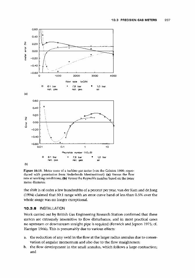
10.3 PRECISION GAS METERS 237
1000
a 61 barnat. gas
2000
flow rate (m3/h)+ 7.8 bar
nat. gas
3000 4000
1.0 bar
(a)
bUJ
-0.20
-0.40
-0.600.01
Reynolds nurrber (10*6)
61 bar + 7.8 bar • 1.0 barnat. gas nat. gas air
(b)
Figure 10.15. Meter error of a turbine gas meter (van der Grinten 1990; repro-duced with permission from Nederlands Meetinstituut): (a) Versus the flowrate at working conditions; (b) Versus the Reynolds number based on the innermeter diameter.
the shift is of order a few hundredths of a percent per year, van der Kam and de Jong(1994) claimed that 50:1 range with an error curve band of less than 0.5% over thewhole range was no longer exceptional.
10.3.6 INSTALLATIONWork carried out by British Gas Engineering Research Station confirmed that thesemeters are extremely insensitive to flow disturbance, and in most practical casesno upstream or downstream straight pipe is required (Fenwick and Jepson 1975; cf.Harriger 1966). This is presumably due to various effects:
a. the reduction of any swirl in the flow at the larger radius annulus due to conser-vation of angular momentum and also due to the flow straighteners;
b. the flow development in the small annulus, which follows a large contraction;and

238 TURBINE AND RELATED FLOWMETERS
c. the integrating effect due to the linear relationship between lift coefficient andincidence for small incidence angles.
They suggested that flow straighteners should only be used upstream if there is apossibility of persistent swirling flow at inlet (cf. Mottram and Hutton 1987).
For inlet flow disturbance, van der Kam and Dam (1993) suggested that the inletflow conditioner could be quite effective in removing swirl, so that swirling flow froma double elbow out-of-plane (with a 40° swirl angle) may not cause errors of morethan 0.3% (cf. Bellinga and Stronk 1974 on the development of a straightener). Alsochange in pipe size before the meter is insignificant. In extreme cases, a tube bundlemay deal with the problem. Roughness does not affect performance. Temperatureeffects are small for a 20° C variation but are difficult to examine due to the lack of asuitable rig. The turbine meter is not suitable for wet or dirty flows. Gases should beclean and free of liquids and dust; otherwise, a filter with 5-/xm filtration quality orbetter should be used. The upstream pipework should be cleaned before installingthe meter (cf. Bonner 1993 and ISO 9951).
According to Harriger (1966), a short-coupled installation with as little as 4Dupstream (2D straightener and 2D straight pipe) is allowable. However, swirl andpulsation can cause significant errors. Meters have a built-in flow straightener, whichremoves some of the swirl. Straightening vanes may be necessary if pipe fittings areat 5D or less upstream. The meter should be carefully centered and protuberancesshould be avoided for at least 5D upstream. Downstream the pipework should be fullbore, but no other restrictions are placed on it. van der Kam and van Dellen (1991)for a 300-mm gas turbine meter suggested that 10D upstream length was sufficientto keep the meter within the limits allowed and 15D if swirl was present.
Excessive speeds can damage the meter, but 20% excess may be allowable forshort periods.
Temperature should be measured downstream within 2D. One manufacturergives a temperature range of -10 to 50°C.
If, as a result of changes in the process conditions, liquid condensate is producedin the pipework, means of drainage should be provided.
10.3.7 SENSINGThe alternative means of measuring the rotation of the wheel are the mechanicalsystem involving a gear train, which can result in retarding forces due to gear losses,losses in the magnetic coupling, and loads from the meter register and calibrationadjustment, or the electromagnetic design in which the loads are much reduced.For a high frequency signal, a proximity switch operating off the aluminum blades,metal strips contained in the hub, or a follower disk on the main shaft, with magneticprobe or proximity switch, allow up to 3 kHz. For low frequencies of 1-10 pulses perrevolution, a reed switch or slot sensor are used.
10.3.8 UNSTEADY FLOWThe gas turbine meter is affected by varying or pulsating flows. The increasing flowcreates higher incidence angles on the turbine blades, and the turbine wheel accel-erates fast. However, when the flow decreases, the blades presumably stall with low

10.3 PRECISION GAS METERS 239
3I
Q
a.
§o
ROTOR SPEED DECAY T IME- t
Figure 10.16. Rotor speed decay curve for no flow [Equation (10. A.. 20)] of a givenmeter during coasting process of the spin test (Lee and Evans 1970; reproducedwith permission from ASME).
retarding force and hence low deceleration. The effect is to give an overestimation ofthe total flow. The turbine bearings may be damaged if subject to fluctuating flowsfor extended periods. Head (1956) gave a pulsation factor, which for turbine meterswas
^ = (l+abF2) (10.8)qv
where qx is the indicated flow rate, qv is the actual flow rate, a = | for sinusoidalvariation of flow, b is taken as unity for nonfollowing meters, and r is full flowamplitude relative to average flow. Head gives r = 0.1 as the practical threshold forsignificant error.
The transient analysis is given in Appendix 10.A.2. From this analysis, a speeddecay curve for no flow is obtainable (Figure 10.16). We can obtain from this curvethe rotor coast time to standstill and the final slope 5 of the curve, which is relatedto the ratio of the nonfluid drag and the inertia and hence to the condition of thebearings. However, de Jong and van der Kam (1993) were doubtful as to its valuefor high pressures. The reader is also referred to the paper by Lee and Evans (1970)who describe how they obtained speed of decay curves using an externally appliedmechanical friction loading method and also gave typical values of inertia (e.g., fora 150-mm low pressure meter with plastic rotor / = 0.242 x 10~3 kg m2 and for ahigh pressure meter with aluminum rotor / = 0.486 x 10~3 kg m2). They also gaverj = 0.2 as used in Appendix 10.A.2.
Lee et al. (1975) obtained the effect of sinusoidal pulsation on errors. Assumingthe worst situation where rotor inertia is too great to follow pulsation, they obtainedfor a pulsation index of 0.1 about 0.5% error and for 0.2 about 2% error where the

240 TURBINE AND RELATED FLOWMETERS
•4
' i
i
1
i
r vmean
•T i m e
E x p e r i m e n tO T = 2 0 SA T = 5 0 SD T = 3 6 0 S
T h e o r y
0 .1 0 . 2 0 .3 0 . 4 0 .5 0 .6 0 .7 0 .8 0 .9
Figure 10.17. Effect of modulating flow on the performance of a 4-in. (100-mm)turbine meter (Fenwick and Jepson 1975; reproduced with permission of BritishGas).
pulsation index is assumed to be given by
= Vmax ~ ^min
Vmax + Vmin
Figure 10.17 is adapted from Fenwick and Jepson (1975) and shows the effect ona turbine meter of a square wave pulsation. McKee (1992) found errors rising fromzero for a 2% variation to 1.5% for 6% and above (cf. Atkinson 1992 who developeda computational analysis of the meter error for near-sinusoidal flow pulsations andCheesewright et al. 1996 who queried the lack of reports of flows with pulsatingwaveforms).
Fenwick and Jepson (1975) gave as an example a 100-mm meter subjectedto on-off pulsations with a period of 60 s resulting in a 40% overregistration (cf.Grenier 1991).
I worked with some data from tests where a gas conversion process requiredvariations in natural gas flows from high to low flow and back with sudden changeand significant errors, which were predicted by the methods of Jepson and others.
10.3.9 APPLICATIONSOne manufacturer claims that its meters can be used with all nonaggressive gasesand fuel gases including town gas, natural gas, refinery gas, coke-oven gas, propane,butane, liquid gas/air mixtures, acetylene, ethane, nitrogen, carbon dioxide (dry),air, and all inert gases.
It is unusual for the turbine meter to be applied to flows of oxygen for the fol-lowing reasons.
a. Any lubricant used must be compatible with oxygen.

10.4 WATER METERS 241
b. A maximum flow rate of order 10 m/s may be specified for oxygen flows inpipework that may oxidize, and this tends to be rather low for a gas turbinemeter.
Pfrehm (1981) described a system adapted from long accepted and accurate liquidmeasurement techniques to the mass measurement of ethylene gas. It consisted ofa meter, density measurement, flow computer, and piston bidirectional pipe prover.The meter is claimed to provide accuracies of ±0.2% with linearity from 20% or lessto 100% of maximum flow.
10 .3 .10 ADVANTAGES AND DISADVANTAGESNewcombe and Griffiths (1973) made the following suggestions.
a. Changes in friction and blade form due to mechanical deterioration or damagereduces the meter's rangeability and gives a slow registration. Filtering limits therate of deterioration, but regular proving tests are required. Spin down tests canindicate bearing deterioration.
b. Rapid flow variations cause the meter to read fast. For a 10 minute off/10 minuteon cycle, one meter read 3% fast.
c. Swirl will affect registration unless a straightener is fitted.d. Registration shifts between low and high pressure operation and, due to high
bearing friction, can be as large as 2%.e. Security of gas flow is not affected if the meter fails.
To these, van der Kam et al. (1990) add reliability, high accuracy, dual measurement,and back-up system in a device with proven technology.
10.4 WATER METERS
10 .4 .1 PRINCIPAL DESIGN COMPONENTS
Figures 10.18(a, b) show diagrams of water meters.A common design of this meter allows for a complete mechanical insert to fit into
a flanged iron section of pipe with a specially made central containment section. Theinsert consists of flow straighteners, which also incorporate the upstream bearing;the rotor, which is usually of helical design and may have a substantial clearancebetween the blade tips and the casing; the rotor shaft, the motion of which is trans-mitted via a right angle worm gear assembly into a watertight gearbox; and a rudder(or trimming vane) upstream of the rotor, which provides a mechanical calibrationadjustment by altering the angle at which the inlet flow stream hits the rotor blades.Water may be allowed to enter the gearbox via a filter, and the calibration rudderadjuster within the gearbox is accessed through the calibration port provided in thetop cover. When the cover is fitted over the gearbox to form a watertight joint, theoutput from the gearbox is transmitted via a magnetic coupling to the totalizingregister of the meter.
Figure 10.18(b) shows a meter in which the shaft is perpendicular to the pipe,providing a simpler transmission but a more tortuous flow path and, presumably,

242 TURBINE AND RELATED FLOWMETERS
Figure 10.18. Diagrams of water meters (reproduced with permission of Meinecke): (a) Gas andWater Meter Manufacturers meter; (b) Gas and Water Meter Manufacturers meter with shaftperpendicular to the pipe.
resulting in a higher pressure loss. Special designs are available (Section 10.4.8), andFigure 10.19 shows one installed on a hydrant.
10.4.2 BEARING DESIGNManufacturers appear to give little information on this. Stainless steel shafts and insome cases stainless steel bearings are used.
Typical submersiblepump installation
Specifiedby customer
Figure 10.19. Hydrant meter (reproduced with permission of KDG Instruments).

10.4 WATER METERS 243
10.4.3 MATERIALSFor temperatures up to 40° C, polythene propellers are suitable, but for meters forhot water, the internals are of hot-water-resistant plastic up to 150°C, and for tem-peratures up to 200° C, the measuring element may be red bronze and the wheel maybe stainless steel. Other materials used are brass and stainless steel.
10.4.4 SIZE RANGEMeters range from 15 to 500 mm. One manufacturer has introduced a dual system,which combines meters of very different capacity and uses a valve to control theflow through the larger meter.
10.4.5 SENSINGThis is usually via a gear train but may also use optoelectrical methods, reed switches,etc.
10.4.6 CHARACTERISTICS AND ACCURACYFigure 10.20 shows a typical operating envelope for a water meter. For the top ofthe range (gtrans to qmax), ±2% is required for a turndown between 11:1 and 5:1,depending on the size of the meter. For the bottom about 3:1 to 7:1 (gmin to quans), therequirement is ±5%. Some values from ISO 4064 and BS 5728 specifications follow:
Size (mm) 50 65 80 100 150qmax (m3/h) 30 50 80 120 300qn (m3/h) 15 25 40 60 150qtrans (m3/h)qmin (m3/h)Starting flow (approx)Head loss at gmax (bar)
4.51.50.340.20
7.520.680.04
81.20.680.09
12100
.8
.91
.08
304.51.590.09
where qmax is the maximum peak flow rate, qn is the recommended continuous flowrate, gtrans is the flow rate at which the uncertainty specification changes, and gmin
is the minimum flow at which the performance is defined.Some commercial designs outperform these requirements, and the reader should
check for ISO updates.
5 -
2o£ 0
-2
-5 -
Figure 10.20. Operating envelope for a water meter based on ISO/BS specifica-tions.
^min <?trons
\\
Operating envelope/
i
On
//
Flow rate
^max

244 TURBINE AND RELATED FLOWMETERS
10.4.7 INSTALLATION
A typical requirement for installation is 5D upstream. In addition, air and solidmatter should be avoided.
10.4.8 SPECIAL DESIGNS
Irrigation and mainline designs are inserted through openings in the pipe, manholes,and saddles or by a bolted flange in a T piece. Accuracy is unlikely to be high. Sizescan be as great as 1,000 mm in diameter.
10.5 OTHER PROPELLER AND TURBINE METERS
10.5.1 QUANTUM DYNAMICS FLOWMETER
One design used a patented twin-turbine configuration whereby the downstreamslave turbine drove the shaft on which the indicator turbine bearings rotate freely.Under normal conditions, the rotational speeds of the indicator and slave turbinesare closely matched. At high flow rates, the rotational speeds of the indicator tur-bine and the slave turbine/shaft assembly will begin to diverge. An integral flow-straightening device upstream of the indicator turbine reduces swirl and hence theeffect of upstream flow distortion. With a special design of RF pickup, claims of±0.01% linearity for a turndown of between 350:1 and 500:1 have been made. Ingaseous flow, these rangeabilities were claimed to correspond to a mass turndownin excess of 1,000:1.
10.5.2 PELTON WHEEL FLOWMETERS
Pelton wheel flowmeters operate like a hydraulic Pelton wheel by using the impulsedue to the fluid jet momentum. To achieve this, the flow is constricted to a smalloutlet and hence forms a high speed jet. A typical design is shown in Figure 10.21.
Pick-off coil casing
Insulator
Soft iron pole pieceRetaining ring
O ring sealCo*l \ 1 /
/
/ \ Bearing/• '—* Flowmeter housing __
Metering plug fc-Figure 10.21. Pelton-wheel-type flowmeter (reproduced wiNixon Instruments).
with permission of

10.6 CHAPTER CONCLUSIONS 245
It is designed for use with liquids. An up-stream filter with a 60-mesh insert may berecommended. A typical low flow range is0.18-1.81/min with a repeatability claimedas ±0.25%. The passing of the rotor tips issensed by a reluctance pickup.
Other designs on the Pelton wheel prin-ciple have also been used to produce meterscapable of flow rates as low as 0.06 1/h to0.75 m3/h with repeatability of ±0.3% ofFSD. Alternatively, they have been used asa bypass flowmeter, which operates acrossan orifice to allow higher ranges.
Vane
Figure 10.22. Vane flowmeter (reproduced withpermission of Fisher Rosemount Ltd.).
10.5.3 BEARINGLESS FLOWMETER
This meter has a floating rotor. After the inlet, the liquid divides and flows upwardand downward past the twin rotors, which are on a common shaft. The flow lifts therotor off its seating because there is lower static pressure in the flow than under therotor. The flow at both ends of the shaft passes the blades on the rotor wheels beforeleaving through two channels that join at the exit. Sensing magnets are sealed intothe rim of the lower rotor, and their passage is sensed by an inductive coil. The basicinstrument has a size range of about 15- to 80-mm diameter with flow range fromabout 0.2 to 5.2 m3/h.
10.5.4 VANE-TYPE FL0WMETERS
Vane-type flowmeters cannot be claimed as high precision instruments. The descrip-tion "inferential," sometimes applied to turbine flowmeters, is probably appropriatefor these meters because the flow of fluid through the meter is inferred from theeffect on the rotor of its interaction with a proportion of the fluid flow.
Figure 10.22 shows a diagram of the principle of operation. The liquid hits thevanes and imparts momentum to them. The clearance between the vanes and thecasing distinguishes this meter from the positive displacement meter and allows thefluid to slip past the vanes on the return.
The flow ranges for this type of meter may cover 0.45 to about 12 m3/h witha maximum pressure drop of about 1.4 bar and a maximum allowable kinematicviscosity of about 48 cSt.
Other devices of a similar type are the angled vane flowmeter with three to fourblades on a shaft angled at about 45°, designed with a removable body, and a furtherdesign operating on the same principle but in the converse way to a paddle wheel.The fluid passing pulls the ridged wheel with it.
10.6 CHAPTER CONCLUSIONS
The considerable range and diversity of this family of designs are shown in thischapter. The one drawback is that with rotation there is often the potential problemof wear to consider, especially for nonlubricating liquids and dry contaminated gases.

246 TURBINE AND RELATED FLOWMETERS
However, against this must be set their extraordinary versatility. Very high accuracy isachieved in some; very large turndown ratio is achieved in others; and suitability fora wide range of fluids and a very wide price range are also features of the family. Newdesigns with extraordinarily great turndown and others with self-checking abilityindicate that the family is far from dying out.
The problem of bearing wear has been controlled but requires that all types ofmeter are subject to regular maintenance, van der Kam and de Jong (1994) claimedthat the gas turbine meter, calibrated at the operational pressure, can be one of themost accurate gas meters available at present and could be used more for custodytransfer. Gasunie have suffered very few mechanical failures (blade failure or dam-aged bearings) and van der Kam and Dam (1993) reckon the turbine meter still thebest option and capable of further development.
Great care must be exercised in ensuring that the installation does not invali-date the calibration. Transient behavior in gases results in an overregistration of theflow. New sensor technologies may lead to lower drag and higher integrity of signal,particularly in adverse radiation environments.
Intelligent designs that build in a self-checking or condition-monitoring facilityare likely to be of particular value for metering high value fluids in fiscal and custodytransfer applications.
Theoretical analysis of flow through the meter should take account of thevery small deflection compared with the substantial deflection that occurs in apower turbine. Ferreira (1988) attempted some computational work on the flowswithin some turbine meters and compared these with LDA measurements. Theresults were interesting and original, but the nature of the flow and the verysmall deflections, which result in the case of a well-designed rotor, suggest thatfuture computations should take account of these features in a perturbation-typeanalysis.
APPENDIX 1O.A
Turbine Flowmeter Theory
10.A.1 DERIVATION OF TURBINE FLOWMETERTORQUE EQUATIONS
Blade AerodynamicsThere are two distinct approaches to the blade forces in the literature. Using cascadetheory, Tsukamoto and Hutton (1985) give the driving force as
rV2zs(t<mp2 -
which equates the torque to the change in angular momentum of the fluid passingthrough the blade row. Replacing px by p - i and p2 by p - 8, and noting that both

10.A.1 DERIVATION OF TURBINE FLOWMETER TORQUE EQUATIONS 247
/ and 8 will be very small, we may rewrite Equation (10.A.I) as
Td = pN I' rV\s [tan(£ - 8) - tan(£ - i)]dr (10.A.2)J
rV\s l t m P S - »±L±) dr (10.A.3)z y i + 5tan£ 1 + i tarijSy v ;
Ignoring terms in is, etc. (1° = 0.0175C),
Td = pN I" rVJs^f^^dr (10.A.4)L z l + (z+5)tan£
or if we ignore (i + 8) compared with unity,
Td = pN I' rV2zs(i - S)(l + tan2 p)dr (10.A.5)
The alternative airfoil theory approach is to use lift and drag coefficients. Theseare given per unit length of the blade by
1 / Vz VL = -pcKcA--^-\ (10.A.6)
where K is the factor that allows for the change in lift coefficient between an isolatedairfoil and a cascade. The torque on the rotor is now given by
Td = 1-pN f * ' 'z c(KCL - tan pmCD)dr (10.A.8)2 Jrh COS^m
This is essentially the term given by Blows (1981) for the aerodynamic lift torqueminus the aerodynamic drag torque. Next, Equations (10.A.2) and (10.A.8) are shownto be equivalent.
Equating the axial force to the force due to change in static pressure:
Z = (pi- p2)s
+• (Poi ~ Poz)s
Equating the tangential force to the rate of change of angular momentum,
Y = pVz2s[tan(p - 8 ) - t an( j8 - /)]
Substituting for V\ and V2, we obtain
Z = -4p^25[tan2G6 - i) - tan206 - 8)] + s(pOi - poz)
= -pVz25[tan(^ - i) - tan(j8 - 8)] tan^m + s(pOi - P02)
We may write the lift in terms of Y and Z as
L = Ycosfim +.

248 TURBINE AND RELATED FLOWMETERS
and, substituting for Y and Z,
-8)L = PV?
So
L = pV?s[tan(j8 - 5) -
and for the drag
- /)] cos£m - PVz2s[t<m(/3 - i) - tantf -
COSp
- /)] sec £m + s(pOi -
and substituting for Y and Z
D = p^2s[tan(£ - 8) - tan(fi - i)] sin^m 4- s(pOi - P02) cos^m
So
^ = 5(^01 -p02)COS£m
Substituting into Equations (10.A.6) and (10.A.7), we obtain
KCL = 2^[tan(£ - 8) - tan(p - /)] sec f5mcos2^m + S-
= — [tan(p -8)- tan()3 - /)] cos pm + CD tan ^m
^ s in^m cos2 /3m
(10.A.9)
where
CD tan An = — sin pm cos2
which shows that Equations (10.A.2) and (10.A.8) are equivalent.
The theoretical expression given by various authors for the lift coefficient is
CL = 2JT sin a
or in fuller form by Batchelor (1967)
CL = 27rsina(l +O.77£B/c)Lift curves are reproduced in Figure 10.9, and drag curves can be found in Wallis
(1961). The angle a is that between the far field and the line of zero lift of the blade,which for a flat plate is the angle with the plate. It appears to be conventional totake the direction of the far flow field for a cascade as the mean direction betweeninlet and outlet and a for a cascade as the angle between this mean direction andthe blade angle (cf. Thompson and Grey 1970). Thus for a cascade of closely spacedflat plates, the exit angle relative to the blades will be zero, whereas the inlet angle

10.A.1 DERIVATION OF TURBINE FLOWMETER TORQUE EQUATIONS 249
will be equal to the far field. Thus the value of a will be half the incidence angle /.So following convention,
CL = 2nsini/2 (10. A. 10)
for the closely spaced flat plates, and, in this limit, according to Weinig (1932):
K = -—-— (10.A.11)c n cos p
Thuss4_sin^5^i
and Equations (10.A.5) and (10.A.8) are identical provided 8 = 0 and CD = 0.For values of sic not tending to zero, we shall find it useful to use the values of K
obtained by Weinig (1932) and given by Wislicenus (1947), and it will be necessaryto write the lift coefficient in terms of the true incidence angle /. From Figure 10.3,
a)= tan pm
so that
but
P-<* = p1
soi + 8
and
CL = lit ( ^ j r ) = n(i + 8) (10.A.13)
and hence
l r~ 2P Jr
rt rV\COSpn
If we make the assumption that both 8 and CD may be neglected in the case of awell-designed turbine wheel, we have
rV2zcK(r)i(r) _,__ , , r t A , r ,
Finally, it is useful to consider the actual values of CD and 8. We can first of allobtain from Equations (10.A.5), (10.A.8), and (10.A. 10)
1 c „ . 5 .2 cos pm cos2 p
K - 2S l
~ Tt C COS Pm

250 TURBINE AND RELATED FLOWMETERS
Then applying this to CD and 8 and making use of Equations (10.A.5) and (10.A. 14),
1 cKn8 1 c „ s82 COS £ m 2 COS /3m
U " m COS2
Hence,
c sin £m
From Wallis (1961), as i tends to zero, CD tends to 0.017. For p = 45° and sic ~ 1,
CD~ 0.017-4^25
so that
8 ~ 0.003c ~ (1/6)°
So if we neglect the drag terms (Equation 10.A. 14),
v * r * * 9 5 _ L * 4 s 8j\7To — L>n tan p m _ z o — —8ccos^m c sin £m
we are actually neglecting
-2-—— ~-0.0085ccosfim
We can compare this with the size of the drive torque
l
C COS An
Thus the neglected term is 8/i of the drive term.
Drag TermsTsukamoto and Hutton (1985) identified four drag torques:
T B , bearing drag;Tw, h u b disk friction drag;Tt, t ip clearance drag;Th, h u b fluid drag.
In t he first three, t he torque is obtained from an equat ion of the form
T = Shear stress x Area x Radius x Reynolds numberx Funct ion of Reynolds number
For instance, for the bearing drag, we obta in
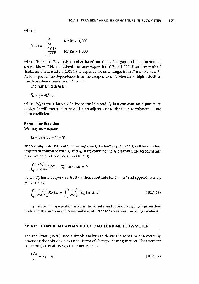
10.A.2 TRANSIENT ANALYSIS OF GAS TURBINE FLOWMETER 251
where
2— for Re < 1,000
f(Re)= R ei i i i i *i
for Re > 1,000
where Re is the Reynolds number based on the radial gap and circumferentialspeed. Blows (1981) obtained the same expression if Re < 1,000. From the work ofTsukamoto and Hutton (1985), the dependence on co ranges from T <x co to T oc co18.At low speeds, the dependence is in the range co to co1-5, whereas at high velocitiesthe dependence tends to co1-75 to co1-8.
The hub fluid drag is
where Wh is the relative velocity at the hub and Ch is a constant for a particulardesign. It will therefore behave like an adjustment to the main aerodynamic dragterm coefficient.
Flowmeter EquationWe may now equate
Td = Tft + Tw + Tt + Th
and we may note that, with increasing speed, the terms TB, Tw, and Tt will become lessimportant compared with 7d and 7h. If we combine the 7h drag with the aerodynamicdrag, we obtain from Equation (10.A.8)
[T' rV7C , r, „,/ —-— (K CL - Cp tan pm)dr = 0
Jrh COS fimwhere CD has incorporated Th. If we then substitute for Ci = ni and approximate C^as constant,
rrt ry2c /Tt ry2c
Jrh COS p m Jrh COSpm
By iteration, this equation enables the wheel speed to be obtained for a given flowprofile in the annulus (cf. Newcombe et al. 1972 for an expression for gas meters).
10.A.2 TRANSIENT ANALYSIS OF GAS TURBINE FLOWMETER
Lee and Evans (1970) used a simple analysis to derive the behavior of a meter byobserving the spin down as an indicator of changed bearing friction. The transientequation (Lee et al. 1975, cf. Bonner 1977) is
^ ^-7, (10.A.17)at

252 TURBINE AND RELATED FLOWMETERS
where the driving torque Td may be obtained from Equation (10.A.I) for one radiusand unit blade length as
Td = pNrVzzs(tan#> -tanfa) (10.A.18)
or, since Vztan^i = rco and putting
T KJ T, (^tariff-ra>)Td = pNrsvz —
where rj allows for the blade deviation factor. Also putting Tr = pAr3Qco2/2 + Tn,where the first term is fluid drag and the second term 7 is nonfluid drag assumedconstant, Lee et al. (1975) then obtained
A-i— + VW + D2W2 = V2 -D3 (10.A.19)dx
where
r2pAV0T
rtanppA2V2
and V = VZ/VO,W= rco/ Vo tan f$ and r = t/T, the fundamental period of the pulsat-ing flow. This equation is soluble on a computer. For certain cases, an exact solutionis possible. Lee and Evans (1970) give the speed decay curve for no flow (V = 0) as
D l / ' " * — ' "l - - t a n - ' " ) (10.A.20)
This curve is shown in Figure 10.16. We can obtain from this curve, as shown byLee and Evans (1970), that the rotor coast time to standstill is
and just before this point
D1^ = -D3 (10.A.22)dx
so that, from the slope 5, we have
5 = - ^ - (10.A.23)

CHAPTER
Vortex-Shedding, Swirl,and Fluidic Flowmeters
11.1 INTRODUCTION
This chapter deals with measurement techniques based on instabilities in fluid be-havior. In preparing this chapter, I benefited from an unpublished note in 1988by Dr. M. V. Morris, of Cranfield University, who drew my attention to some earlyreferences on this type of meter.
11.2 VORTEX SHEDDING
The detailed behavior as fluid flows past a cylindrical bluff body is given in Ap-pendix 11 .A. 1 in relation to the size of the Reynolds number based on the diameterof the cylinder. Figure 11.1 shows the development of the flow past such a bluff bodyuntil, at a Reynolds number of about 40, the familiar shedding phenomenon starts.However, small changes of detail in the pattern of the shedding are illustrated by thediagram for certain Reynolds numbers. Frequency changes occur at these Reynoldsnumbers. These changes could result in nonlinearity and poor repeatability in ameter.
Figure 11.2 is a simple diagram to suggest how, as a vortex rolls up downstreamof a noncircular bluff body, it first forms, fills with rotating fluid, and then draws influid with opposite rotation, which eventually cuts off the vortex and allows it tomove downstream. In Appendix 11.A.2 a simple argument is used to suggest thatthe frequency of shedding f is about
f=V/2nw (11.1)
where V is the velocity past the body of width w. An important parameter, theStrouhal number, is given by
S= fw/V (11.2)
This relationship has been applied to long slender cylinders. Our applicationis to the vortex-shedding flowmeter where the flow is in a pipe and the width ofthe shedder (bluff body) is between a quarter and a third of the pipe diameter, andthus is not a long slender cylinder. However, as we shall see, this length/width ratiois advantageous in terms of the strength of vortex shedding and leads to coherentshedding, whereas longer and more slender shedding bodies result in weaker andless coherent shedding.
253

254 VORTEX-SHEDDING, SWIRL, AND FLUIDIC FLOWMETERS
40 < Re < 150 (e) 300<Re<3x10⁵ (f) 3x10⁶<Re<107
Figure 11.1. Flow patterns around a cylindrical body: (a) For Re < 4; (b) Initiation of separationfor 4 < Re and up to about Re = 30; (c) Lack of separation symmetry behind cylinder for about30 < Re < 40; (d) Stable and viscous shedding for 40 < Re < 150; (e) Stable shedding withturbulent shear layer for 300 < Re < 3 x 10⁵; (f) Stable shedding with turbulent boundary andshear layers for 3 x 10⁶ < Re < 107.
11.3 INDUSTRIAL DEVELOPMENTS OFVORTEX-SHEDDING FLOWMETERS
The use of this instability for velocity measurement was recognized at an early stage(cf. Roshko 1954) and has led to its use in flowmeters and probes, (cf. Medlock 1976).
Most modern meters use bluff bodies that are not circular in cross-section andthat have a sharp shedding edge to remove the shifts resulting from changes in theboundary layer. Coherent shedding appears to take place along the length of thebluff body if the length (in this case the diameter of the pipe) is in the range ofabout 2.5 to 4 bluff body widths (Zanker and Cousins 1975). By coherence we meanthat the vortex is shed from end to end of the bluff body on the same side at thesame time.
(a)
Figure 11.2. Diagram of vortex formation behind a bluff body: (a) Start of forma-tion of new vortex; (b) Opposite vorticity starting to be entrained; (c) Oppositevorticity breaks and separates vortex.

11.3 INDUSTRIAL DEVELOPMENTS OF VORTEX-SHEDDING FLOWMETERS 255
For a cylindrical bluff body, it is found that the strength of the force caused bythe vortex shedding is greatest when D/w is about 2.8 because the shedding becomesmore coherent and enhanced. By this means, the shedding becomes approximatelytwo-dimensional. For a flowmeter where the shedder spans the pipe, it is advan-tageous if its width is about a quarter of the pipe diameter. The wall of the tubethen acts as end plates for the shedder and encourages coherent and strong vortexshedding. Coherence and stability of the shedding range has been achieved downto about Re = 104, where the Reynolds number is based on bluff body width (cf.Takamoto and Komiya 1981 who described a positive feedback system to extend therange below Re = 2,000).
In flow measurement, strong pressure pulsations caused by the shedding willenhance the signal, resulting in easier detection of shedding.
Three-dimensionality in the flow stream (e.g., turbulence, velocity gradients,and swirl) has detrimental effects on the quality of the vortex shedding (Zanker andCousins 1975, cf. El Wahed and Sproston 1991 and Robinson and Saffman 1982).Except in carefully controlled conditions, a slender cylinder in the flow will createvortex shedding, which varies in strength and phase along its length (cf. Saito et al.1993).
11 .3 .1 EXPERIMENTAL EVIDENCE OF PERFORMANCE
The vortex flowmeter, therefore, consists of a bluff body, usually of noncircular cross-section, spanning the pipe and having a width of a quarter to a third of the pipediameter (Figure 11.3). Zanker and Cousins (1975) provided a useful review of earlywork on vortex flowmeters (cf. Tsuchiya et al. 1970 and Cousins et al. 1973) and thevarious effects that take place.
As the body becomes thicker (w increases) and the velocity past the body, there-fore, increases for a fixed volumetric flow rate, Equation (11.1) suggests that the
SENSOR CONNECTION
FLOW TUBE
FLOW
BLUFFBODY
Figure 11.3. Diagram of vortex flowmeter.
SHEDVORTICES

256 VORTEX-SHEDDING, SWIRL, AND FLUIDIC FLOWMETERS
co 1000
800
600
<400
(a)
[\ AVPRACTICAL
u u
h-
-W02—iQIdu-0 1O U Jtoo
/°/X
X
i i i
XX
i i i
01 02 03 04 05 06w/D
01 02 03 04 05 06w/D
(b)
Figure 11.4. Pulses per unit volume and lift force for cylindrical bodies (from Zanker and Cousins1975; reproduced with permission from NEL): (a) Pulses per unit volume against blockage ratio;(b) Lift coefficient against blockage ratio.
frequency and hence the pulses per unit volume of fluid may change. We shall referto this ratio as the K factor (see Section 1.4). Figure 11.4(a) for a cylindrical bluffbody shows this factor reducing to a minimum at a w/D of about 0.35. When w isof order 0.1D, the strength of the lift coefficient is low [Figure 11.4(b)]; but when ithas the value 0.35D, it is at a peak. Zanker and Cousins suggested that this strengthwas due to two effects that fortunately occur together:
• coherent shedding due to the shorter length of the bluff body between the endplates of the wall of the tube;
• the accelerating flow through the smaller space between the body and the tubewall, leading to a more uniform profile and less dependence on the upstreamflow profile.
An important reason for the choice of the minimum is that small variations inw/D have a minimal effect on the frequency.
The constancy of the meter factor is shown in Figure 11.5 for a Reynolds numberrange of nearly 1,000:1 with air and water where the scatter was usually within±0.5% (Zanker and Cousins 1975). White et al. (1974) gave a calibration curve
E 2430rAUDIBLECAVITATI0N
10 8 105 2 A 6 8PIPE REYNOLDS NUMBER
106
Figure 11.5. Typical calibration curve for a 3-in. (75-mm) vortex meter (from Zanker and Cousins1975; reproduced with permission from NEL).

11.3 INDUSTRIAL DEVELOPMENTS OF VORTEX-SHEDDING FLOWMETERS 257
for a 3-in. (75-mm) meter in air over a 360:1 turndown (with a lower Reynoldsnumber of 104) and showed that scatter was of order ±1% over the range. A majorproblem in achieving this size of turndown is how to sense at the varying levelof signal. If velocity changes by 100:1, then pressure head variation due to thevelocity will change by 104 : 1 . Goujon-Durand (1995) confirmed that a minimumReynolds number of Re = 30,000 is probably necessary to avoid serious increase innonlinearity. Takahashi and Itoh (1993) showed a slight decrease in Strouhal number(about 2%) from Re = 20,000 to Re = 50,000 for heavy oil, water, and air.
Inkley et al. (1980) obtained data to show the small effect of temperature changethrough viscosity and density on the meter. Change of liquid and liquid viscosityappears to have caused calibration shifts of order 0.5%. If the meter is designed closeto the minimum in Figure 11.4(a), any variation due to temperature expansion willbe minimized. The major change was due to cavitation. The authors agreed withWhite et al. (1974) that a universal curve should be obtainable and foreshadowedthe work of Takamoto and Terao (1994) and, no doubt, others.
11.3 .2 BLUFF BODY SHAPE
Figure 11.6 shows the effect of body shape on the optimum value of w/D and alsoshows that the K factor decreases from the value for circular bluff bodies. The trun-cated triangular or trapezium shape appears to be best if length to width is in therange 1.2 to 1.5. The rectangular body with length to width about 0.6 may havestrong shedding.
Lucas and Turner (1985) confirmed that a splitter plate attached to the bluff bodyimproved signal quality, which, presumably, is the reason for the T and truncatedtriangular body shapes.
El Wahed and Sproston (1991) experimented with various bluff body shapesin air. The sensing used a modulated signal from naturally occurring flow-inducedstreaming currents. The shedder shapes are shown in Figure 11.7. The shedders hadend plates to create two-dimensional conditions. The main conclusions were thatthe best position for the sensor was attached to the front face of the bluff body andthat:
1000
800
600
£00
200
CIRCULAR CROSS-SECTION
EQUILATERAL TRIANGULAR•EASTECH DESIGNKI DESIGN
0-1 02 03 0A 0-5 06w/D
Figure 11.6. Optimum w/D for various body shapes (from Zanker and Cousins 1975; reproducedwith permission from NEL).

258 VORTEX-SHEDDING, SWIRL, AND FLUIDIC FLOWMETERS
Figure 11.7. Shedder shapes tested by El Wahedand Sproston (1991) (reproduced with permission ofElsevier Science Ltd.).
• the cylinder with a slit was slightly bet-ter than the solid cylinder (cf. Igarashi1986);
• the rectangular shedder produced a highsignal-to-noise ratio suggesting that thebody produced a large drag, which inturn encouraged the vortex to sweepacross the rear face, reinforcing and sta-bilizing the shedding; and
• the T-shaped shedder was the best, sug-gesting that the tail helps control theshedding and produces a high signal-to-noise ratio, which is approximately con-stant throughout the entire range.
Figure 11.8 shows the cross-section of various bluff body shapes that have beenused in flowmeters. Bentley and Nichols (1990) suggested that, for a thin plate, thevortex field is much farther downstream than for a square. The shape in Figure 11.8(g)may result in a considerable amplification of the vortex strength and hence of thepressure variation.
There appear to be mixed views on the use of composite shapes (cf. Majumdarand Gulek 1981 and Herzl 1982). The conditions for optimum shedding from dualbodies (Bentley and Benson 1993) relate to
• the thickness-to-width ratio of the two bodies;• the spacing of the bodies; and• the positions of maximum vorticity.
For dual bluff bodies, the movement of the boundary layer through the gap isessential for vortex enhancement. There are two options (Bentley et al. 1996) forposition of a second bluff body: either the second body is far enough away forthere to be shedding from both, or the second is less than a critical spacing, which
(a)
(d)
(f) (g)V
(h)
Figure 11.8. Diagrams of cross-section of bluff bodies (some after Yamasaki 1993and some from manufacturers' brochures).

11.3 INDUSTRIAL DEVELOPMENTS OF VORTEX-SHEDDING FLOWMETERS 259
leads to shedding taking place downstream of both, with greater shedding stability.Bentley et al. identified certain spacing, which appears to be preferable, but thesmall size of the spacing between bodies may present a problem in small metersizes.
It is interesting to note that the dual bluff body is essentially providing a feedbackpath between the two bodies of fixed dimensions and so, presumably, defining thevolume needed to fill the feedback path and the time in a more stable way, hence thegreater stability. Tests by Bentley and co-workers suggested that this is still furtherenhanced by introducing a throat in the gap, by making the downstream body adouble wedge with the vertex pointing upstream.
Some manufacturers' designs allow the replacement of the sensor without clos-ing down the line. One that uses a dual bluff body (essentially a triangular shapefollowed by a piezoelectric sensor mounted outside the flow line on a symmetricalwing airfoil that senses the downstream pressure variations) provides for the piezocrystal's accessibility during operation.
Turner et al. (1993) proposed a new body shape (cf. Zanker and Cousins 1975) forvortex-shedding flowmeters, consisting of a cylinder split across its lateral diameter,with a concave rear surface. They claim a high signal-to-noise ratio and an almostconstant Strouhal number over a wide Reynolds number range. Miau et al. (1993)described a T-shaped vortex shedder consisting of a trapezoidal bar of fixed shape,with a rear plate whose length can be varied. The optimum length of plate was foundto be in the range 1.56-2.0 times the width of the vortex shedder. They obtained aturndown ratio of about 17:1.
One manufacturer (at least) offers a triple body. The outer bodies (cylinders)create the vortex street, and the center body senses the vortices. It should give similarperformance for flow in both directions.
11.3 .3 STANDARDIZATION OF BLUFF BODY SHAPE
Takamoto and Terao (1994) have taken a basic design of bluff body of the truncatedtriangle type (Figure 11.8b). Figure 11.9 shows the essential dimensions, and the pa-per sets out the tolerance on these and the tolerance with which the body should beset. Thus, a selection of the dimensions and tolerances (rounded to reduce significantfigures in some cases) are given in Table 11.1. The alignment refers to the orientationof the bluff body relative to the axis of the pipe. The perpendicularity is relative tothe pipe diameter. This is a very interesting development, which appears to stem
Table 11.1. Selection of dimensions and approximate permitted error for astandard flowmetera
DimensionValueMaximum
errorEffect on
^-factor (%)
w/D
0.280.1%
0.13
H/D
0.350.7%
0.09
h/D
0.036.6%
0.13
L/D
0.9120.15%
0.08
e19°0.4°
0.05
Alignment0°0.5°
0.05
Perpendicularity0°0.3°
0.06
a Refer to the original paper by Takamoto and Terao (1994) for precise values.

260 VORTEX-SHEDDING, SWIRL, AND FLUIDIC FLOWMETERS
(b)
Figure 11.9. Diagram to show the main dimensions for a proposed standard(after Takamoto and Terao 1994): (a) Cross-section of bluff body; (b) Cross-section of pipe.
mainly from Japan. It is interesting to note that the flow area is close to that foran orifice of p = 0.65. In their tests, the value of H/D ranged from 0.20 to 0.40for w/D = 0.28, and the Strouhal number varied by about 8% for this range. Theirresults also suggest that H/D = 0.35 results in a Strouhal number, which only variesby about 1% for a range of Reynolds number from 2 x 10⁴ to 106.
11.3 .4 SENSING OPTIONS
A major limitation of the meter is the transducer; consequently, various sensingmethods have been tried, and all have advantages and disadvantages. Some of thesemethods include:

11.3 INDUSTRIAL DEVELOPMENTS OF VORTEX-SHEDDING FLOWMETERS 261
• Ports in the sides of a bluff body as in Figure 11.8 (a, b) leading to a transverseduct, which allows movement of fluid to be sensed by an internal hot wire or athermistor;
• Temperature variation to sense changes by attaching thermistors to the upstreamface of a bluff body such as that in Figure 11.8(b) or Figure 11.8(d);
• Pressure on lateral (electrical capacitance) diaphragms that deflect [Fig-ure 11.8(e)];
• Pressure on a small diaphragm in the side of the bluff body [Figure 11.8(f)];• Pressure sensed through ports in the sides of the bluff body [as for Figures
11,8(b, d)], or downstream of the bluff body in the fluid or in a symmetrical wingairfoil. The pressure changes create very small bending of a sensitive element (atlow flows the tip may be moving by as little as 3 x 10~8 m). This movement caneither be measured by strain gauge or by capacitive methods.
• Flexure of whole or part of the bluff body [Figure 11.8(h)] measured with straingauges;
• Flexure of the whole bluff body sensed by strain gauges in the end supports ofthe body;
• A shuttle ball in an internal cavity in the bluff body linked by ports to the fluid,with movement sensed by magnetic induction [Figure 11.8(b)]; and
• A beam of ultrasound, crossing the flow downstream of the bluff body, modulatedby the vortex shedding.
Pressure is the most common variable to be sensed, evidenced by: ports in thebluff body, pressure sensor built into the bluff body surface, flexible diaphragm,forces on the body, movement of a shuttle in the body. Thermal sensors are alsoused, built into the body and affected by fluid flows. Fluids should be clean andnoncorrosive.
A new design of meter using ultrasonic sensing appears to operate successfully.Optical sensing may offer a further alternative (e.g., in the form of optical fibers inthe bluff body).
Takahashi and Itoh (1993) described a design that used the alternating lift onthe shedder, which is sensed through two piezoelectric elements [Figure 11.10(a)].By using two sensors, effects due to vibration of the pipeline are reduced. A stablezero is created by using the strength of the vortex-shedding signal (proportional top V 2) and creating a low flow cutoff when this does not tally with the value of V fromthe vortex-shedding frequency. Another arrangement is shown in Figure 11.10(b);here the vortices lead to a small flexural movement of a section of the shedderbar, and a piezoelectric element inside the sensor senses this minute movement.Figure 11.10(c) shows the position of a sensor bar, which can be inserted into orplaced downstream of the shedder body.
Herzog (1992) used optical fibers within the bluff body of a vortex-sheddingflowmeter to sense the frequency. One fiber appears to have been subject to thetransverse forces through ports in the body, whereas the other was totally en-closed. The bending of the first fiber caused changes to the quality and inten-sity of the light, and both speckle pattern and intensity were used to obtain thefrequency (cf. Hisham Marshad and Irvine Halliday 1994 and also Wen Dong-Xu1990).

262 VORTEX-SHEDDING, SWIRL, AND FLUIDIC FLOWMETERS
Leadwires
Pipe Line (body)
Direction of Flow
(a)
PiezoelectricSensor Element
Figure 11.10. Commercial designs of flowmetersensing systems: (a) Basic construction and vortexshedder bending moment diagram showing signalcomponents 5 and noise components N (repro-duced with permission of Yokogawa Europe B.V.);(b) Shedder bar/sensor operation (reproduced withpermission of Fisher-Rosemount Ltd.); (c) Sensorpositions (reproduced with permission of Bailey-Fischer and Porter).
Sensor
(c)
Sproston et al. (1990) experimented with electrostatic sensing, and in later testsEl Wahed and Sproston (1991) used electrostatic sensors as shown in Figure 11.11,either in the walls, behind the body, or on the front face of the body. The mechanism,on which this sensing is based, is that charge is produced in flows (flow-inducedstreaming currents), and so its variation can be used to measure flow variation. Theexperiments were in air.

11.3 INDUSTRIAL DEVELOPMENTS OF VORTEX-SHEDDING FLOWMETERS 263
Piezoelectric elements may be sensitiveto pipe vibration and degrade the signal-to-noise ratio. Stiffening the meter body,using filtering and a low cutoff (Kawanoet al. 1992) may partially overcome theseproblems.
Figure 11.12 shows a block diagram fora signal converter.
11.3.5 CROSS CORRELATION ANDSIGNAL INTERROGATION METHODS
Coulthard and Yan (1993a) suggested theuse of the vortex wake as a tracer foruse with cross-correlation techniques. Thebluff bodies that were used presented a lowblockage to flow and appeared to give sim-ilar accuracy to those of vortex-sheddingfrequency measurement. This presumablyindicates that the cross-correlation tech-nique is capable of the same discriminationas the frequency measurement electronics.Coulthard and Yan (1993b) investigatedthe effect of various bluff body shapes butfound little difference between them (how-ever, cf. Terao et al. 1993).
Amadi-Echendu et al. (1993) describeda further piece of work to analyze the rawsignal from a flowmeter, in this case a vortex
'///////
iV//////////////777.
V77///////////Y7
Figure 11.11. Electrostatic sensor positions (ElWahed and Sproston 1991; reproduced with permis-sion of Elsevier Science Ltd.).
Electronics module
Piezoelectricsensor
Anti-aliasingfilter
Analog-to-digital signalconversion
Galvanicisolation
I '-z ~l
Digitaltracking
filter ASICGalvanicisolation
Microprocessor• Transmitter
configuration• Temperature
correction• Diagnostics• Rerange
Display• 8 digit• Engineering
units• ConfigurableI • configurable
Pulse
Digitalcommunication
Digital-to-analog signalconversion
Figure 11.12. Block diagram of electronics module for commercial flowmeter (after Fisher-Rosemount Ltd.).

264 VORTEX-SHEDDING, SWIRL, AND FLUIDIC FLOWMETERS
flowmeter, to ascertain information beyond pure flow information. It is not clearfrom this paper the extent to which this will be possible. Clearly condition moni-toring from this source would be very valuable. However, there is a need to link thefrequency data as closely as possible to the physical effects so that the changes canbe intelligently used (cf. Section 10.2.16 and a note in Chapter 21).
11.3.6 OTHER ASPECTS RELATING TO DESIGN AND MANUFACTURE
Itoh and Ohki (1993) claimed (as does one manufacturer) a vortex flowmeter design,which obtains mass flow rate by using the lift on the central body divided by thefrequency of pulsation. This depends on the assumption that the lift coefficientand the Strouhal number are both constant so that the lift is proportional to pV2,and the frequency is proportional to V. As a result, the ratio is proportional to p V(cf. Yamasaki 1993).
Miller et al. (1977) gave some impressively consistent K factors from the produc-tion process showing random uncertainty in K of order ±0.8% for 50-mm meters,±0.4% for 75-mm meters, and ±0.3% for 100-mm meters.
11.3.7 ACCURACYTypical performances of meters currently available are given as: repeatability, about±0.2% rate; linearity, better than ±1% for a turndown ratio of up to 40:1 for liquidsand up to 30:1 for gases. For liquids at higher flow rates, the uncertainty appears tobe in the range 0.5-1% of rate. At low flow rates, it is the same range of values but asa percentage of full-scale deflection. The change will be at about Re = 20,000, witha minimum value of Re of about 4,000 and upper limit of about 7 x 10⁶. The typeof transducer may affect the low flow limit.
For gases and steam, the uncertainty appears to be in the range 1-1.5% of rate,but with Re < 20,000 likely to increase uncertainty.
Temperature variation is likely to affect precision, and compensation may beincluded (e.g., 0.3%/50°C).
Cousins has commented that it is necessary to collect a large number of pulsesto achieve good repeatability due to variation of 10-20% in the shedding period. Asa consequence, long integration times should be expected.
11.3.8 INSTALLATION EFFECTS
Table 11.2 shows the change in error for increasing installation lengths (Takamotoet al. 1993b). Some of the results suggest that the error does not always decrease withspacing. The worst case has been used, from the results of four meters.
Mottram (1991) commented that 'The difficulties of deciding what should be theminimum straight pipe length between a given type of flowmeter and a particularupstream pipe fitting are notorious. Even when the geometry is standardized, as isthe case for the sharp edged orifice, the issue is still controversial. This is due to thetypical shape of the envelope enclosing the experimental results for the calibrationshift plotted against the straight pipe length separating the meter from the upstreamfitting. Minimum straight lengths may differ by a factor of two." Mottram;s tests werefor a vortex meter with an area ratio approximately equivalent to a ft = 0.6 orifice

11.3 INDUSTRIAL DEVELOPMENTS OF VORTEX-SHEDDING FLOWMETERS 265
Table 11.2. Results from Takamoto et al. (1993b) that appear to give the worstcase uncertainty (rounded up to the first decimal place) at various spacings
2x Bend (%)
5D10D20D30D
Bend90° (%)
1.90.60.40.3
SamePlane
2.10.70.40.2
90°Plane
2.11.10.80.6
Reducer(%)
0.90.70.30.3
Expander(%)
4.21.40.30.3
Gate Valve Open (%)
100%
0.30.40.40.3
50%
5.11.50.50.4
area ratio. We compare in Table 11.3 Mottram's and Takamoto et al.'s (1993b) valuesfor the vortex installation lengths and those from ISO 5167 for orifice meters withp = 0.6 and £ = 0.75.
Mottram gave a general rule that vortex sensitivity was similar to that for ahigh beta ratio orifice plate. This would appear to be a reasonable working rule ofthumb from his results and is in close agreement with Ginesi and Annarummo (1994)who suggested using the 0.7 beta ratio lengths. However, Mottram's comment thatminimum lengths may differ by a factor of two is borne out by Takamoto et al.'s(1993b) results.
Further results from Mottram and Rawat (1988) (using a rectangular bluff bodyand hot-wire anemometer probe to detect the vortices) suggested that pipe wallroughness, presumably resulting in profile changes, can cause 3% variation in cali-bration (cf. Witlin 1979).
If we compare manufacturers' requirements, they are fairly consistent in suggest-ing 5D downstream although at least one suggests 10D, but for upstream spacing,
Table 11.3. Installation lengths (diameters) between upstream fitting and meter forchanges within ± 0.5% compared with spacing for orifice
2x Bend
Bend Same 90°90° Plane Plane Reducer
Gate Valve OpenExpander 100%
22
16
19
38
14
5
12
24
50%
3016
—
Orifice - zero additional uncertainty£ = 0.6 18 26 48 9Vortexa 55 60Vortex6 13 12 43 14Orifice - ± 0.5% additional uncertainty£ = 0.75 18 21 35 11Orifice - zero additional uncertainty£ = 0.75 36 42 70 22a Mottram's (1991) meter with blockage equivalent to £ = 0.6.b Takamoto et al.'s (1993b).

266 VORTEX-SHEDDING, SWIRL, AND FLUIDIC FLOWMETERS
Table 11.4. Installation requirements (inmanufacturers' literature compared with
90° bend or T2 bends
in same planein perpendicular planes
ReducerExpanderValvea
Downstream spacing
Orifice (3 =(±0%)
18
2648
92226
7
diameters) as indicated inorifice plate requirements= 0.6
Vortex
10-20
20-2530-4010-2010-4020-50
5-10
Orifice (3 = 0.75(±0.5%)
18
2135111918
4a Globe valve fully open.
they give values as in Table 11.4. These are, again, compared with orifice spacings, forp = 0.6 ratio orifice (zero additional uncertainty) and p = 0.75 ratio orifice (±0.5%additional uncertainty).
Apart from the valve, the values in Table 11.4 suggest that to take the greater ofthe spacings for a p = 0.6 orifice with zero additional uncertainty and for a ft = 0.75orifice with ±0.5% additional uncertainty might provide a rule of thumb for otherfittings. There appears to be a more severe effect due to reducers and expanders,about which some manufacturers are clearly cautious. Further, although this is inline with Takamoto et al. (1993b), it does not cover the more pessimistic resultsof Mottram (1991), and for safety we may need to accept his guidance that theinstallation distance should be that for zero additional uncertainty with p = 0.75(or 0.8), accepting Mottram's factor-of-two observation.
Manufacturers have warned against the protrusion of gaskets into the flow up-stream and adjacent pipe bores of different size to the meter. The inlet pipe shouldbe free of weld beads and thermometer pockets and should be smooth; the pipeworkshould be aligned with the meter. Takahashi and Itoh (1993) suggested \% error forinstallation in a pipe of different bore to the meter, and one manufacturer gives theeffect as less than 0.6% for a step of 4-10% greater than the flowmeter ID resultingfrom the pipe schedule.
Cousins (1977) commented on the severe effect of swirl in changing the cali-bration and even in suppressing the shedding and suggested at least 50D upstreamspacing from the source of the swirl for a swirl angle of 10° and more spacing forlarger angles. However, Laneville et al. (1993) showed that, for swirl indices (Q =injected swirling flow rate/total flow rate) less than 0.3, the vortex-shedding signalquality from a vortex flowmeter with trapezoidal body is equivalent to the zero swirlcase, and the frequency is still within about 2% of the swirl free value for a spacing18D downstream of the swirl generator. These apparently differing results will callfor caution.
Pressure taps downstream should be 2D to 7D, and temperature taps shouldbe ID to 2D downstream of the pressure ones. A flow straightener of 2D length
11.3 INDUSTRIAL DEVELOPMENTS OF VORTEX-SHEDDING FLOWMETERS 267
separated by 2D from the disturbance should have 5D to the meter. Mottram (1991)obtained good results using a Mitsubishi conditioner with a different spacing. For abend, 90° offset bends, orifice plate with £ = 0.645, and fully open globe valve, hisresults were within a band of ±1% with 5D between the fitting and the conditioner,2.5D between the conditioner and bluff body, and 2.5D downstream of the bluffbody.
Other mounting constraints are not usual, but pipework must ensure that themeter runs full.
11.3 .9 EFFECT OF PULSATION AND PIPELINE VIBRATION
It is known that vortex meters may be affected by pulsatile flow, particularly wherethe pulsating frequency or its harmonics are close to the shedding frequency. Themeter may lock on to the pulsation frequency and give an error (cf. Amadi-Echenduand Zhu 1992). Some sensing techniques may be more susceptible to error due topulsation than others. Some may be designed to select the shedding frequency byeliminating pulsation or vibration using a push-pull arrangement.
Hebrard et al. (1992) confirmed that pulsations can cause large metering errors.Pulsations of an amplitude of only a few percent may be sufficient to produce meter-ing errors, particularly when the frequency is near the fundamental or first harmonicof the shedding frequency. The lock-on frequency is most likely to occur when thepulsation frequency is twice the vortex-shedding frequency, and lock-on can occur(Al-Asmi and Castro 1992) even down to pulsation amplitudes of about 2%. Outsidethe lock-on range, there can still be significant differences between the sheddingfrequency in steady and pulsating flows, and free stream turbulence may increasethe problem.
Manufacturers may suggest that disturbances upstream of an unsteady natureshould be given a wide berth. Malard et al. (1991) found that there was an increaseof about 2% and a decrease in the signal-to-noise ratio when the turbulence intensityincreased from 3.3 to 10.3%. Their work also confirmed the errors due to pulsatileflows.
As indicated earlier, sensors are designed to minimize the effect of pipeline vibra-tion, and the manufacturer should be consulted for information. However, processnoise may cause zero flow signals but may be diagnosed by looking at the raw signal(Ginesi and Annarummo 1994).
11.3.10 TWO-PHASE FLOWSHussein and Owen (1991) found that the correction factor for the vortex meterfor wet steam of high dryness factor is closest to the value x~1/2 (Figure 11.13). BS3812:1964 is quite close. Pressure was shown to have little effect on correctionfactors. Hussein and Owen (1991) gave the wise advice that an upstream separator isadvisable, and that there are several types giving a value of x > 95% with reasonablylow pressure loss.
The possibility that the meter might be developed to sense the droplets of wetsteam is an interesting challenge for the signal processing experts.

268 VORTEX-SHEDDING, SWIRL, AND FLUIDIC FLOWMETERS
1.10
U. 1.05
31-00
0.95
0.90
0.85
vortex-sheddingmeter
BS 3812:1964
0.84 0.88 0.92 0.96Dryness fraction x
1.00
Figure 11.13. Comparison between wet steam correc-tion factors for vortex meters (after Hussein and Owen1991).
The meter has virtually the samecalibration for liquid and gas flows andmight therefore be expected to behavewell in two-component flows. Howeverthe published work highlights some severeproblems.
The first is that the components areseparated by the vortex motion. Hulin et al.(1982, 1983) found that shedding in ver-tical water-air flow was stable up to about10% void fraction. They also found that thevortices trap bubbles [Figure 2.9(b)] withan associated decrease in the strength ofthe pressure fluctuations. Their later workon water-oil flows shows some contrasts.The separation is much more completefor water-air due presumably to the den-sity difference, and this leads to a muchnarrower vortex emission bandwidth. Thestability at oil concentrations greater than
30% was notable, and the cores of the vortices were continuous oil.The second is that the bubbles may trigger certain sensors. Baker and Deacon
(1983) obtained results suggesting that, even though vortex-shedding continuedwith increase in void fraction in a vertical upward water-air flow, bubble impactmay cause additional pulses. Above air volume concentrations of 1%, the metererror increased by more than 1% for each additional 1% air concentration.
A third problem, to which Washington (1989) attributed poor results in wet gas,may be slip between the components. A homogeneous second component in theflow may be measured but will usually result in a loss of accuracy due, in part, to thefact that the instrument measures the volumetric flow.
11 .3 .11 SIZE AND PERFORMANCE RANGES AND MATERIALSIN INDUSTRIAL DESIGNS
As indicated earlier, the low end is limited by Reynolds number behavior, and theeffect of Equation (11.1) is that, as the size increases, the frequency becomes verylow and makes the meter unusable.
Diameter ranges from about 12 to 200 mm or more are quoted by various man-ufacturers. Flow rates through the meters are up to about 9 m/s for liquids and75 m/s for steam and gas. Flow ranges for liquids may be from a minimum of lessthan 1 1/s to a maximum of about 600 1/s and for gases 15 1/s or less to 3,000 1/s ormore.
Range is of order 20:1 on gas and steam and 10:1 for liquids (up to 60:1 issometimes given). This creates a constraint with the minimum Re, which may inhibitits application where the precise range is unknown or spans two meter sizes. Inothers, a smaller-sized meter may be necessary to cope with the range. Overrangingup to 20% is generally allowable, but the low flow end may be more due to thestrength of the signal.

11.3 INDUSTRIAL DEVELOPMENTS OF VORTEX-SHEDDING FLOWMETERS 269
Minimum Reynolds number is variously given as 3,800-5,000, although metersmay be of lower accuracy below 10,000 and upper limits of 500,000 and up to orgreater than 1,000,000 may be given.
Viscosity should be below 8 cP (the viscosity of cooking oils), although it maybe possible to measure with reduced range up to 30 cP (Ginesi and Annarummo1994). A low flow cutoff is usually set somewhat below Re = 10,000, and this maybe a disadvantage for some applications.
The temperature range may be from less than -200° to over 400°C. Pressure maybe up to 150 bar or more depending on the transducer. Pressure drop on a meterof nominal internal diameter equal to the pipe is normally less than about 40 kPa(6 psi) on water flow.
Pulse rates will vary enormously depending on the size of the meter. For a smallmeter of about 20 mm diameter, the rate will be of order 200 pulses/1, whereas fora large meter of 300 mm diameter the rate will be of order 0.02 pulses/1. Responsetime may be of order 0.2 s or three shedding cycles for a change to 63% of input.All this may be affected by resolution problems when combined with poor periodrepeatability.
Material of the bluff body is most commonly stainless steel but may be titaniumor another material.
Vortex meters, like turbine meters, are limited at the upper end of their range bypossible cavitation. Casperson (1975) suggested the possibility of hysteresis effectsdue to cavitation and the need to avoid operating in this regime. To avoid cavitationin liquid flows, some manufacturers give a formula of the following type for theminimum back pressure 5D downstream:
Pgmin = AAp + Bpv - patmos
where Ap is the pressure drop across the meter, pv is the saturated liquid vaporpressure, and patmos is the atmospheric pressure. A appears to have a value of about3.0, and B has a value of about 1.3. Ap is of order 1 bar at 10 m/s.
These meters may, also, be subject to compressibility effects.
11 .3 .12 COMPUTATION OF FLOW AROUND BLUFF BODIES
Some early work obtained good agreement between numerical and experimentalresults for Re up to 1,000 for confined two-dimensional flows around rectangularcylinders (Davis et al. 1984). More recent work by Matsunaga et al. (1990) showedsome impressive computer-generated flow patterns around a trapezoidal body in atwo-dimensional flow. Comparison of Strouhal number obtained computationallyand experimentally agreed quite well at Re > 1,000 but appear to diverge for lowerRe and were less good for Re of order 10,000. Figure 11.14 shows the vortex-sheddingmechanism as interpreted by the authors.
Johnson (1990) computed the unsteady laminar flow around a cylinder and ob-tained agreement within 10% for the Strouhal number in comparison with experi-mental values for part of the range. Computer simulations by El Wahed et al. (1993)again obtained good agreement with the experimentally acquired Strouhal numberand indicated that the T-shaped shedder produced the largest vortex.

270 VORTEX-SHEDDING, SWIRL, AND FLUIDIC FLOWMETERS
• Upper flow
(a)
(b) \—s
(c) Inletflow
(d)
(e)
Figure 11.14. Flow pattern behind shedder: (a) t = 1.2615 s; (b) t = 1.2660 s;(c) t = 1.2690 s; (d) t = 1.2735 s; (e) t = 1.2765 s (after Matsunaga et al. 1990;reproduced with permission of Elsevier Science Ltd.).
11 .3 .13 APPLICATIONS, ADVANTAGES, AND DISADVANTAGES
Furness and Jelffs (1991) sought to make a case for using vortexmeters to measureflows in and out of refineries rather than depending on tank transfer. Proving, how-ever, may be problematic due to the poor period repeatability.

11.3 INDUSTRIAL DEVELOPMENTS OF VORTEX-SHEDDING FLOWMETERS 271
Siegwarth (1989) discussed tests on specially designed vortex-shedding metersfor application to very high flow rates of liquid oxygen in the space shuttle mainengine ducts. The details of this work may be of interest to those engaged in vortexflowmeter design.
The claims of manufacturers for applications include
• liquid flows (e.g., liquid N2, CO2, O2, clean liquids, distilled water, glycol, someacids, low viscosity hydrocarbons, benzene, diesel, hydraulic oils, creosote, andtar),
• gas flows [e.g., steam (superheated and saturated) and various gases includingcompressed air, methane, N2, and CO2], and
• cryogenic applications, but not multiphase applications.
In general Yamasaki (1993) saw the meter as an alternative to the orifice meter,provided it could cover a similar range of fluid parameters. (One manufacturer claimsthat costs are about 50% of those for orifice plates.) The sensing method is the mainconstraint to extending parametric range. However, temperature range now allowsits use with superheated steam and liquid natural gas (LNG).
11 .3 .14 FUTURE DEVELOPMENTSThere is a need to extend the range of the vortex meter, to improve application data(e.g., installation effects), and to develop the signal processing.
Zanker and Cousins in their work as long ago as 1975 foresaw the dual bluff body,and, no doubt, there is further development possible in the design of these bodies.They also mentioned annular ring/coaxially mounted bluff bodies, and Takamotoand Komiya (1981) also proposed such a ring-shaped bluff body that sheds ringvortices.
Miau and Hsu (1992) surveyed the flow around axisymmetric disks and rings asvortex shedders, showed the pattern of vortex loops behind a disk, and were par-ticularly interested in the flow characteristics near the pipe wall, suggesting thatan advantage of the axisymmetric designs is that the sensing can be on the pipewall. Axisymmetric vortex-shedding rings intuitively offer an elegant axisymmmet-ric version of the meter. Tai et al. (1993) discussed optimum size and positioningand signal-to-noise ratio. Cousins and Hayward (1993, cf. Cousins et al. 1989) de-scribed developments of the vortex ring flowmeter and discussed sensing options.They made the point that ring vortices are far more stable than those from straightbluff bodies. They suggested that a ring/pipe diameter ratio of 0.4 is about optimum.They found that the signal-to-noise ratio varies markedly across the pipe and downthe centerline, peaking at 3 to 4 ring widths downstream. They found that the innerring vortices give a clearer signal. The provisional design, which appears to be opti-mal is a double ring with a tail; it appears to give a repeatability of ±0.1% or betterwith only 0.3 velocity head pressure loss.
The combination of electrostatic sensing as described by El Wahed and Sproston(1991) with ring vortex shedders could be very attractive. The sensor could be in thewall of the tube or even at various points to give greater intelligence to the meterand forms of self-monitoring.

272 VORTEX-SHEDDING, SWIRL, AND FLUIDIC FLOWMETERS
11.4 SWIRL METER - INDUSTRIAL DESIGN
This section is concerned with the industrial design of the swirl meter, which hassome fluid behavioral similarities to the vortex whistle (Chanaud 1965). In the whis-tle, initial swirl is created by tangential flow into an upstream plenum from whichthe helical vortex emerges.
11.4 .1 DESIGN AND OPERATION
A diagram of this type of flowmeter is shown in Figure 11.15. As the flow enters themeter, inlet guide vanes cause it to swirl. As the flow moves through the contraction,the angular momentum created by the guide vanes is largely conserved, and so theangular velocity will increase. The vortex filament develops into a helical vortex,as shown in the diagram, which moves to the outside of the tube. The frequencywith which the helix passes the sensor provides a measure of the flow rate. Theflowmeter section then expands, and the swirling jet at the wall surrounds a regionof reverse flow on the axis. This motion is removed before the fluid leaves the meterby means of a deswirler. Dijstelbergen (1970) explained the precession as being dueto the increasing pressure in the diffusing section causing a force on the exitingswirl, which is converted to a lateral momentum change. Ricken (1989) gave furtherdetails of a model to describe the behavior of the meter.
Heinrichs (1991) described a sensing system for a swirl meter in which the rota-tion is sensed by using two diametrically opposed pressure ports. In the measuringtube of the swirl meter, a helix-shaped vortex appears, rotating with a frequencyproportional to the volumetric flow rate. In this way, the differential pressure elimi-nates common mode signals and hence the problem of a high line pressure and flow
Preamplifier
SwirlerDeswirler
Figure 11.15. Swirl flowmeter (after Bailey-Fischer and Porter with their per-mission).

11.4 SWIRL METER - INDUSTRIAL DESIGN 273
fluctuations. The push-pull arrangement suggests that the range may be extended.Capacitive sensors seem to be less suitable, whereas the results for piezoelectric onesare more promising.
11.4.2 ACCURACY AND RANGESAn industrial design has been available for liquids, gases, or steam with vortex ro-tation frequency obtained using piezosensors. Measurement uncertainty of betterthan 1% of rate is claimed by the manufacturer over the upper 80% of the range forthe smaller sizes, with better than 2% for the 10-20% part of the range. For sizesabove 32 mm, uncertainty of better than 1% of rate is possible over the upper 90%of the range.
Flow ranges are, for liquids, from 0.2 to 2 m3/h up to 180 to 1800 m3/h and,for gases, from 5 to 25 m3/h up to 1000 to 20,000 m3/h. Values for steam should beobtained from the manufacturer. Turndown for some sizes for liquids is up to about30:1, and for gases it is between 5:1 and 20:1. Maximum frequencies range forliquids from 100 Hz for a 20-mm-diameter meter to 13 Hz for a 400-mm meter andfor gases from 1200 Hz for meters of 20 mm down to 150 Hz for a 400 mm diametermeter. A 10% overranging is allowed in gases, but in liquids cavitation must beavoided. Maximum velocity is 6 m/s for liquids and 50 m/s for gases.
For liquids at the top of the flow range, pressure loss can range from about 200to 400 mbar or more, and for gases the range is from 25 to 70 mbar or more. Theflowmeter is available in designs suitable for hazardous area use.
11.4.3 MATERIALSThe material in contact with the liquid is predominantly stainless steel, except forthe thermistor sensor in gases, which is glass-insulated and epoxy-potted, and thepiezosensor, which is stainless steel or some other material.
11.4.4 INSTALLATION EFFECTSFor bends, contractions, and valves upstream, the recommendation is for 3D straightpipe before the inlet flange; for bends and expansions downstream, it is ID. How-ever, a contraction downstream is not permitted. For large radius bends, etc., therequirements may be further reduced.
The manufacturer appears to claim low sensitivity to fluid pressure, temperature,and density. Fluid temperature is -40 to 280° C.
Maximum viscosity is 70 mPas. Deposits can cause errors, but it may also tendto self-clean. Cavitation must be avoided with liquids by ensuring adequate staticpressure.
11.4.5 APPLICATIONS, ADVANTAGES, AND DISADVANTAGESThe meter is recommended by the manufacturer for applications where absolutereliability with minimum maintenance is essential and is claimed to be suitable forwet or dirty gases and liquids. Specific applications are water, sludge water, conden-sate, acids, solvents, petrochemical raw materials, gasoline, air, CO2, natural gas,ethylene, and steam.

274 VORTEX-SHEDDING, SWIRL, AND FLUIDIC FLOWMETERS
11.5 FLUIDIC FLOWMETER
The third instability we consider is that for the fluidic flowmeter. A diagram of atypical design is shown in Figure 11.16. The fluidic flowmeter uses the Coanda effect.If a two-dimensional diffuser has too wide an angle, the flow will separate and attachto one wall of the diffuser. It may attach to either wall and can be displaced fromone to the other by a suitable disturbance. The fluidic flowmeter introduces sucha disturbance, which causes the flow to oscillate between the diffuser walls at afrequency proportional to the velocity of flow. There are several parallels with thevortex meter. Types of sensors used in vortex flowmeters could be applied to thisdevice. There is likely to be room for design optimization. The flow range may bewide, and certainly the device looks promising for low flows.
The mechanism by which the flowmeter operates is that the flow, having at-tached to one wall, passes into a feedback channel. The fluid when it exits from thischannel knocks the main jet to the other side of the diffuser, and the process startsagain. Thus the period is related to the time for the flow to move from the entryof the flowmeter to the entry of the feedback channel and communicate, via thatchannel, to the entry. This time will be inversely proportional to the velocity of flow,and so the oscillating frequency will be proportional to the flow rate.
11.5 .1 DESIGN
Boucher and Mazharoglu (1988) developed one design of fluidic target meter, whichoperated down to Re of about 70 but with considerable change in Strouhal numberat low Re. Hysteresis may have a small effect in starting and stopping (cf. Boucher1995).
Sanderson (1994) described a new fluidic water meter using electromagneticsensing. This is a particularly appropriate method with a wide dynamic range and alinear response to flow rate. It is also usable in a constant magnetic field design dueto the fluctuating nature of the flow. The sensing electrodes were made of stainlesssteel, and earthing electrodes were also provided. The magnetic materials consideredfor this device included sintered ferrite and bonded and sintered neodymium. Thegeneral configuration is shown in Figure 11.17. Sanderson's preferred arrangementof magnetic sensor was for the measurement to take place in the main jet with
, Feedbackpath
Oscillatingjet
Inlet • ^ '.'.'""" ( • Outlet
Figure 11.16. Diagram of a fluidic flowmeter (reproduced with permission ofProfessional Engineering Publishing).

11.5 FLUIDIC FLOWMETER 275
magnetic material in the diffuser walls giv-ing a field strength of about 0.3 T. The twopairs of electrodes were in the side walls act-ing 180° out of phase in a push-pull arrange-ment. Over most of its range, the meterwas linear to within ±2% (from about 5 to500 ml/s). Further linearization was possi-ble within the electronic circuitry. The me-ter operated from a 3.6-V lithium batterywith a 10-year lifetime.
Sakai et al. (1989) described a dual sens-ing system gas flowmeter for domestic usein Japan. It was designed to operate from3,000 1/h down to 150 1/h with a piezoelec-tric differential pressure sensor and seemsto have achieved ±2.5% for 150-600 1/hand ±1.5% above 600 1/h. For the range3-1501/h, an integrated circuit thermal sen-sor was used. This had a heated area with
Magnetic material
Backing piate
Electrode
Figure 11.17. Fluidic flowmeter with magnetic sens-ing (Sanderson 1994; reproduced with permission ofElsevier Science Ltd.).
temperature sensor areas on each side of the integrated circuit chip. The character-istic of this sensor appears to have a varying coefficient, and it is not clear whatfinal precision was claimed for low flows. Sakai et al. saw the prospect of using onelithium battery of 5,000 mAh, which would last 10 years in continuous service bylowering the consumption of the circuits.
Measurement accuracy of a preproduction gas meter on field tests in Japan isclaimed (Yamasaki 1993) to be within ±1.5% of reading with a 30:1 turndownratio. Upper flow limits are defined by the allowable loss in the meter. Computersimulation was used as an aid in the design.
Nishigaki et al. (1995) used LDA methods to obtain the flow patterns in a flu-idic gas flowmeter and concluded that the patterns were almost the same across aReynolds number range from 291 to 2,160.
The development of a meter for various Japanese gas companies (Aoki et al.1996, Sato et al. 1996) has included numerical analysis. It has a more complicatedarray of internal bodies with a U-shaped initial target. A 60:1 turndown appearedto be achieved.
11.5 .2 ACCURACYOkabayashi and Yamasaki (1991) found that accuracy could be improved by
i. optimizing the shapes of the side walls and the position of the target andii. incorporating a flow straightener to make the jet two-dimensional.
They claimed a linearity of ±0.8% of reading within the range 0.15-5.0 m3/hwith a repeatability of ±0.2% of reading. The frequency appeared to be about20 Hz/m3/h. Sensing was by a piezoelectric sensor (using a polymer piezoelectricfilm) that does not consume power and an amplifier with very low current con-sumption.

276 VORTEX-SHEDDING, SWIRL, AND FLUIDIC FLOWMETERS
11.5.3 INSTALLATION EFFECTS
It seems likely that these devices will be virtually insensitive to upstream distur-bance because the inlet duct within the meter will have changed section and will beequivalent to several diameters. There is also likely to be flow straightening.
11.5.4 APPLICATIONS, ADVANTAGES, AND DISADVANTAGESThe prime application of these devices is for utility flows where they meet require-ments of
• small size,• large turndown,• low power, and• long life without maintenance.
With no moving parts and compact size, these devices should show advantagesover existing meters for utility (water and gas) flows. However, the sensing range willrequire capability for large turndown if the fluid turndown range is to be realized.
11.6 OTHER PROPOSED DESIGNS
A wake oscillation was observed by Mair (1965). With an axially symmetric andstreamlined body followed by a disk, the wake gathers in the cavity and puffs outregularly. With a torpedo-shaped body of diameter D, a coaxial disk of diameterd, and spacing x downstream of the flat rear of the body, Mair found that withx/D ~ 0.5 and w/D ~ 0.8 the vortex was trapped between the body and the diskand resulted in a low drag, whereas for x/D ~ 0.3 and w/D ~ 0.8, a high drag andoscillation occurred, which he attributed to breathing of the cavity.
Parkinson (1991) described a combination of a venturi nozzle with a folded flu-idic flowmeter (Figure 11.18). Boucher et al. (1991) also designed a folded versionof the fluidic flowmeter to create a bypass for a venturi meter (cf. Wang et al. 1996).In this way, the fluidic principle can be applied to pipes in the range 40-150 mmwith turndown ranges of 24:1 to 40:1. The sensing in the fluidic flowmeter was bymeans of a miniature air-flow sensor on a silicon chip based on thermal convection.
Shakouchi (1989) demonstrated an alternative geometry of fluidic meter wherea rectangular jet issues into a larger space. The oscillating vane meter was discussedin Section 8.8.
11.7 CHAPTER CONCLUSIONS
The vortex meter offers a very attractive alternative to the orifice plate for some appli-cations and gains over the orifice plate by its frequency output and larger turndown.Its application to dry saturated steam may prove to be one of the most importantcontributions of this device. It would be interesting to explore means of sensing, byimpact or by entrainment in the shed vortices, the amount of water in the flow andthus to obtain a dryness factor.

11 .7 CHAPTER CONCLUSIONS 277
Folded fluidic oscillator
Pipe Flange Venturi throat Venturi tailpiece
Figure 11.18. Combined venturi nozzle with a folded fluidic flowmeter (fromParkinson 1991; reproduced with permission of the Institute of Measurementand Control).
The prediction of performance, the effect of inlet flow and turbulence level, andthe means of sensing are areas for development. These will require consideration ofoptimum geometry and, in the case of the vortex flowmeter, the axisymmetric bluffbody.
Much of the computational fluid dynamics (CFD) work has concerned two-dimensional solutions. The axisymmetric vortex body should lend itself to this, butthe straight vortex body in a circular pipe may call for more of an understanding ofhow upstream distortion and turbulence distribution feed into the creation of theshed vortices. There may be some useful analytical work that would shed light onthis and might lead to a weight function for the meter.
The sensing systems are somewhat limited. Pressure, force, etc., have problemson turndown. Temperature sensing may offer scope for some applications. However,the electromagnetic solution is very attractive for liquids, and as well as applicationto fluidic flowmeter, I have, for some time, felt that the vortex flowmeter could becombined with a magnetic flow tube to give self-checking possibilities.
An elegant solution for gases is still awaited, and the development of suitablesensors is an unresolved problem. Should thermal be checked? Does the electrostaticoption provide a solution?
At a more pedestrian level, but of great practical value for the vortex meter,would be further comparative installation effects of commercial meters, togetherwith tests on the effect of pipe size difference, nonalignment, weld beads, etc., andalso vibration. This might be combined with the development of a standard vortex-shedding meter as foreshadowed by Takamoto and Terao (1994).

278 VORTEX-SHEDDING, SWIRL, AND FLUIDIC FLOW METERS
The fluidic meter appears to have found a particular niche in the utilities, andseveral are being, or have been, developed. They appear to offer a large turndown,provided a suitable sensing system is available. One such system is the magneticsystem developed (Sanderson 1994) for water flows.
The CFD analysis of the fluidic flowmeter is also, mainly, two-dimensional, butthe effect of end walls and the turbulence level of the inlet flow may need fur-ther assessment, and it seems unlikely that the internal geometry has been finallyoptimized.
At the opposite extreme would be the investigation of intrinsic flow noise dueto vortex shedding in existing pipework, which could be sensed and calibrated as aflowmeter system. If such noise exists, an intelligent sensor could learn its calibrationand then provide for a utility measurement.
The continuing development of these meters in terms of range, reliability, lowmaintenance, accuracy, and price should ensure that they establish a respected placein the options for flow measurement.
APPENDIX 1 1.A
Vortex-Shedding Frequency
11.A.1 VORTEX SHEDDING FROM CYLINDERS
Flow around a cylindrical body develops as in Figure 11.1. At a low Reynolds number[Figure 11.1 (a)], the flow pattern on each side of the cylinder is almost symmetrical(for Re < 1 there is symmetry cf. Tritton 1988). The symmetry between the flowapproaching the cylinder from upstream and that leaving it downstream is removedwith increasing Re. When Re exceeds about 4 (Tritton 1988), eddies, which are moreor less symmetrical [Figure ll.l(b)], are formed behind the cylinder and, as shownin Figure ll.l(c), start to become unsymmetrical before a Reynolds number of about40 is reached. It is from this point that we obtain the remarkable phenomenon ofvortex shedding.
The lack of symmetry in Figure ll.l(c) breaks down into a periodic flow asillustrated in Figure ll . l(d). At this stage, the flow is stable and viscous (Roshko1954). The boundary layer on the cylinder and the shear layer in the wake are pre-sumably laminar. The shedding is very regular in this region. In the range omittedfrom Figure 11.1, namely 150 < Re < 300 (or 200 < Re < 400 according to Tritton),transition from laminar to turbulent takes place in the shear layer, and the transi-tion is accompanied by less regular shedding. Once the regime in Figure ll.l(e) isreached, the shedding becomes regular once more. A further transition in the region3 x 105 < Re < 3 x 10⁶ occurs as the boundary layer changes from laminar to turbu-lent causing irregularity (Tritton 1988). In this case, Tritton illustrates the laminarseparation followed by turbulent reattachment and then, again, the occurrence ofseparation. The regime in Figure ll.l(f) has regular shedding and a later separationpoint. Tritton comments that markedly periodic shedding remains a characteristicof the flow up to the highest values of Reynolds number at which observations havebeen made, about 107.

11.A.2 ORDER OF MAGNITUDE CALCULATION OF SHEDDING FREQUENCY 279
11.A.2 ORDER OF MAGNITUDE CALCULATIONOF SHEDDING FREQUENCY
Using a numerical solution, Abernathy and Kronauer (1962) showed that two shearlayers result in the build-up of large vortex regions. Their diagrams also showedthat one shear layer gets caught in the other shear layer and eventually resultsin a region where vortices of opposite sense cancel each other and break theshear layer (cf. Robinson and Saffman 1982 on the stability of Karman vortex ar-rays).
Figure 11.2 is a simple diagram of this mechanism (cf. Figure 11.14). In Figure11.2(a), one vortex has just separated and the next is beginning to roll up. The roll-up is caused by the influence of each new vortex on those that have gone before.In Figure 11.2(b), the large vortex roll has curled back on itself and has started toentrain the vortex sheet of opposite sense on the other side of the body. In Figure11.2(0), this entrainment has advanced to the point where the upper vortex sheet isnullified and the roll-up of the vortex is stopped as the whole vortex roll is set free(cf. Gerrard 1966).
A simple model to obtain a value for the roll-up time of the large vortex is givenby Figure 11.A.I. The vorticity shed will be of order V/8, where 8 is the shear layerthickness. The rate of shedding will be approximately the mean velocity in the shearlayer V/2 multiplied by the layer thickness 8. Thus vorticity shedding rate is
V 8V _ V2
J X T~TThe vorticity has to fuel a vortex with a diameter approximately equal to the size
of the bluff body. The total vorticity within this roll will be
V x V •
Vds
= TTWV
The time to fill a vortex of diameter w with nw V is approximately
TTWVT =
V2/2
Thus an order of magnitude value for the frequency again isV
f = 2TTW(11.A.1)
Vorticity
Figure ll.A.l. Simple model of vortex shedding.

280 VORTEX-SHEDDING, SWIRL, AND FLUIDIC FLOWMETERS
A useful parameter is the Strouhal number given by
5= fw/V (11.A.2)
and using the approximation of Equation (ll.A.l) we obtain a value of 5 = l/(27r) =0.16. Goldstein (1965) gave 0.18 for a circular cylinder at a Reynolds number in therange 300-100,000.
Because of the reduced cross-section of the flowmeter due to the presence of abluff body, the actual velocity past the body Vmax will be greater than that in theupstream pipe V. For an incompressible fluid, area x velocity is constant. The arearatio will be given approximately by
A
Thus for an incompressible fluid
Vmax 1
V 1 - 4W/TTD(11.A.4)
and so combining Equations (11.A.2) and (11.A.4) and assuming the appropriatevelocity for Equation (11.A.2) is Vmax, we obtain
45 1(H.A.6)= VrP (w/D)(l-4w/jrD)
and so the approximate Strouhal number of 0.16, which we obtained based on theflow past the body will apparently be increased if based on the velocity in the mainpipe according to Table ll.A.l. For comparison, Takamoto and Terao (1994), for aw/D of 0.28, give S in the range 0.245-0.265 for Re from 105 to 106. The limitationsof this simple approximation are shown by the effect of change in length of the bluffbody from 0.4D to 0.2D found by Takamoto and Terao.
Zanker and Cousins (1975) assumed that the roll vortex was slightly larger thanthe bluff body diameter by between about 10 and 50%. This created a vena contractaconfining the flow downstream of a sharp-edged bluff body to a smaller area nearthe wall in which the maximum velocity increases more. Adding their factor K toEquation (11.A.6), we obtain the same equation as they did:
f _ 45 1Table l l .A.l . Approximate variation of : ^ ~ ^~Q3 (W/D)(l - AKw/nD)Strouhal number based on mean pipe a n 1 A 7velocity for various body sizes
. , It is arguable that a further K shouldW/D linux/V 5 corrected appear as a multiplier in the denomina-o.l 1.15 0.18 tor to allow for the larger vortex, which0.3 1.62 0.26 r has to be filled. However, this is proba-0 5 2-75 °-44 '. bly stretching a simple model too far, but
. . interestingly it appears that for a w/D of

11.A.2 ORDER OF MAGNITUDE CALCULATION OF SHEDDING FREQUENCY 281
about 0.3, this extended form of the denominator is less affected by the value of Kthan for, say, 0.1 or 0.5.
One can see how the change in the upstream conditions could influence theshedding frequency. Upstream disturbances will alter the vorticity in the flow andso reduce or increase the frequency of shedding and possibly the regularity. Thesechanges are illustrated by Mottram (1991) for the effect of a more peaky profile dueto pipe roughness and an increased Strouhal number. In this case, both the increasein local velocity at the body and the increase in vorticity will have effects. Otherresults discussed in this chapter show, surprisingly, that this type of meter is quitesusceptible to the effect of a reducer upstream, presumably again because of theeffect on the turbulence spectrum.
Terao et al. (1993) made two interesting observations.
• Vortices moved faster downstream than the mean velocity.• Areas of intense vorticity existed at the wall.
The first of these two must affect the use of vortex shedding with cross-correlationtechniques. The second suggests that three-dimensional computational solutionsmust include this observation (cf. Majumdar and Gulek 1981 for an early paper onshedding from various prisms).

CHAPTER 1S
Electromagnetic Flowmeters
12.1 INTRODUCTION
The possibility of inducing voltages in liquids moving through magnetic fields wasknown by Faraday in 1832, but the first flowmeter-like device was reported byWilliams in 1930. The first real advance in the subject came from the medical fieldwhere Kolin (1936, 1941) introduced many ideas that are now standard practice.
The industrial interest in electromagnetic flowmeters (sometimes referred to asEM or magnetic flowmeters) grew in the 1950s with
• the Tobiflux meter (Tobi 1953) in Holland for rayon viscose, sand and water, andacid slurries;
• Foxboro, to whom the patent was assigned in 1952;• the first commercial instruments in 1954 (Balls and Brown 1959).• nuclear reactor applications;• the work that resulted in an essential book by J. A. Shercliff (1962).
In this chapter, we shall concentrate on the application of the flowmeter to fluidsthat are of low conductivity, such as water-based liquids (Baker 1982). The flowmeterhas also been used with liquid metals (Baker 1969, 1970b, 1977), and a few designshave been built for use with nonconducting dielectric liquids (Al-Rabeh et al. 1978).The reader is referred to the original papers because space prevents their inclusionhere. Three papers by Wyatt (1961, 1977, 1982), a pioneer in blood flow measure-ment research, are referenced for those interested.
12.2 OPERATING PRINCIPLE
We start with the simple induction, which occurs when a conductor moves througha magnetic field. Figure 12.1 shows a copper wire cutting the flux of a permanentmagnet. The wire is moving in a direction perpendicular to its length and per-pendicular to the magnetic field with velocity V, and the result is a voltage gen-erated between its ends of value BIV where / is its length and B is the magnetic fluxdensity.
Figure 12.2 shows a diagram with the essential features of an electromagneticflowmeter. The liquid flows in a circular cross-sectional tube. A magnetic field is cre-ated across the pipe, usually by coils excited by an alternating current. The tube itself
282

12.2 OPERATING PRINCIPLE 283
must be made from nonmagnetic materialso that the magnetic field can penetratethe tube. In this diagram, we may imaginefilaments of liquid spanning the tube fromone electrode to the other and movingthrough the magnetic field at differentspeeds generating voltages between theirends as was the case with the copper wire.To avoid these being shorted out, thetube is lined with an insulating material.The voltages in the liquid are measuredbetween electrodes, which are set in thewall of the tube.
Referring now to Figure 12.3, we havedepicted the case where more than one wireis moving through the magnetic field. Wire P is in a region of strong magnetic field Band has a velocity V. Wire Q is in a region where the field is about the same size, butit only has a velocity V/2. Wire R, although moving with velocity V, is in a region ofweak magnetic field, say, B/4. Thus the magnetic induction in each will be different:
Figure 12.1. A wire moving through a magnetic fieldgenerates a potential difference between its ends.
InPInQInR
A£/P = BIVAL/Q = BlV/2Al/R = BlV/4
(12.1)
Now if the ends of the wires are connected, currents will flow because the po-tentials differ, and the result will be that A£/P will be reduced by the ohmic loss.Carrying this same argument back to Figure 12.2 results in a complicated pictureof voltages and circulating currents. Despite this apparent complexity, the actualoperating equation of the flowmeter is quite simple for a range of conditions. Thevoltage between the electrodes is given by
AL/EE = BDVm (12.2)
Tube
Flow
Electrodes
Magnet
Figure 12.2. Simple flowmeter.

284 ELECTROMAGNETIC FLOWMETERS
Figure 12.3. Three wires moving through a magneticfield of varying spatial strength at different speeds.
where B is the magnetic flux density intesla, D is the diameter of the tube in me-ters, and V is the mean velocity in the tubein meters per second.
This is the basic equation for the flow-meter, and it can be shown to be valid onlywhen
• the magnetic field is uniform and• the velocity profile is axisymmetric.
In modern designs, these requirementsare seldom satisfied, and so designs have been developed to give an output signal thatis as little affected by the flow profile as possible, in compact designs with magneticfields far from uniform.
12.3 LIMITATIONS OF THE THEORY
Uniform Field - It can be shown that in theory the only field that is uniform isone from a magnet of infinite extent.
Axisymmetric Profile - All fully developed pipe flow profiles are axisymmetric.But it is not always convenient to allow the necessary upstream pipe length toensure a fully developed profile.
Shercliff (1962) suggested a means of predicting the effect of distorted profilesusing what he called a weight function (Appendix 12.A). He calculated the shapeof this function for a uniform magnetic field meter [Figure 12.4(a)]. In its simplestform, this indicates how important the flow is in any part of the pipe cross-sectionand how great its influence will be on the flow signal. The velocity at each pointin the cross-section of the flowmeter is multiplied by the weight function. Thus theweighting function of 2 near the electrodes will cause the flow in that part of the pipeto have twice the influence on the signal. If all the flow went past that point, and theflow everywhere else was stationary, the signal would be twice as big as it should be.
This important concept has been extended by Bevir (1970) and Hemp (1975)and has proved a very useful method of assessing the performance of this and othertypes of flowmeter.
However, Figure 12.4 compares the distribution due to Shercliff with others.Figure 12.4(b) shows the distribution for flowmeters with rectangular-shaped coils, acommon design. Figure 12.4(c) shows the distribution for flowmeters with diamond-shaped coils with their corners along the axis of the pipe and toward the electrodes.These are quite similar to some commercial designs, and the plots of weightingfunctions can be seen to give a much more uniform distribution, particularly in thediamond-shaped case.
Another approach that has been used is to introduce large electrodes that havean integrating effect on the signal and again improve the theoretical performance.Figure 12.4(d) shows an example of a large electrode meter, and it can be seen that

12.3 LIMITATIONS OF THE THEORY 285
ELECTRODE
ELECTRODE
ELECTRODE (d)
Figure 12.4. Weight functions: (a) For a uniform field point-electrode flowmeter (Shercliff 1962);(b) For a point-electrode flowmeter with rectangular-shaped coils and circular yoke (Al-Rabehand Baker 1979); (c) For a point-electrode flowmeter with diamond-shaped coils and circularyoke (Al-Rabeh and Baker 1979); (d) For a large electrode flowmeter with rectangular-shapedcoils and rectangular yoke (Al-Khazraji and Baker 1979).
the weight function over most of the cross-section varies only between about 0.75and 1.6 (cf. Al-Khazraji and Hemp 1980).
For further details on the development of this meter and for additional references,see Baker (1982, 1983, 1985) and Hemp and Sanderson (1981). A thorough reviewof operating problems was provided by Cox and Wyatt (1984).
The effect of short magnetic fields causing nonuniformity of field results in thekind of shorting taking place between P and R in Figure 12.3, which was calledend-shorting by Shercliff. If we define a value S, the flowmeter sensitivity, by
S =Voltage generated
BDVm(12.3)

286 ELECTROMAGNETIC FLOWMETERS
we find that 5 = 1 for Equation (12.2), but for a field length equal to the pipediameter, it falls to about 0.8.
12.4 DESIGN DETAILS
Figure 12.5 shows the main components of an industrial flowmeter with point elec-trodes. The industrial flowmeter is a combination of two elements - the sensor orprimary element and the transmitter or secondary element.
The sensor or primary element consists of the metering tube with insulating liner,flanged ends, coils to produce a magnetic field, and electrodes. In addition, somemeans to produce a reference signal proportional to the magnetic field is usuallyprovided. On AC-powered systems, this has, typically, been a current transformer,or search coil. On DC systems, it may be appropriate to measure the excitationcurrent while constant.
The transmitter or secondary element, which is sometimes known as the con-verter,
a. amplifies and processes the flow signal;b. eliminates spurious electromotive forces;c. ensures that the transmitter is insensitive to electricity supply variation, radio
interference, etc;d. must have the required level of safety; ande. communicates with the user's control computer in the most efficient way.
12.4 .1 SENSOR OR PRIMARY ELEMENT
The metering tube (Figure 12.6) will usually be nonmagnetic to allow field pen-etration. It may be available in a range of diameters from about 2 mm to about3000 mm (10 ft). Flow ranges may be from 0 to 28,500 m3/h or more. The insidesurface is insulated to prevent signal shorting. Electrodes are positioned at oppositeends of a diameter perpendicular to, and central in, the magnetic field. They are typi-cally small (5-20 mm diameter) and are sometimes referred to as point or button
FIELD.COIL
PRIMARYELEMENT
FLOW SIGNAL CABLE
Figure 12.5. Main details of an industrial meter.

12.4 DESIGN DETAILS 287
I1- FLANGE AND TUBE
* INSULATINGLINER
1 ELECTRODES
Figure 12.6. Metering tube.
electrodes. Large electrodes have been used in a few designs, and these may subtendabout 90° and approach one diameter in length.
Typical materials for insulation are given in Table 12.1. The material is oftenmolded around the tube end forming a composite with the flanges. Too high ve-locities [i.e., greater than 4 m/s (15 ft/s)] may lead to liner wear, which can be re-duced with liner protection (Ginesi and Annarummo 1994). Grounding/earthingrings have been used in the past, where the pipes were lined or nonconducting, toprovide a reference point for the measuring electrodes. In modern designs, refer-ence plates or electrodes, which are not necessarily earthed, may be provided. Anearth link could, where the liquid is carrying an electric current, provide a track to
Table 12.1. Liner materials with an indication of approximate temperaturelimits that should be checked with the manufacturer
Material Application Temperature Limits (°C)
Natural rubber
Neoprene
TeflonEbonite
FluorocarbonPolyurethaneElastomerPolyurethane
Polytetrafluoroethylene (PTFE)
Ceramic 99.9% alumina(AI2O3) with cermet(Pt—AI2O3) electrodesmoulded in before firing
Wear and chemical -20 to 70resistance
Good chemical and 0 to 100wear resistance inpresence of oil andgrease
Abrasion and chemical 0 to 90resistance
Slurry
Wear and impactresistance
Wear resistance,chemically inert,good for foodstuffs
- 5 0 to 70
- 5 0 to 200

288 ELECTROMAGNETIC FLOWMETERS
earth and cause galvanic damage. In this case, the meter may be allowed to floatelectrically and would be made safe via an isolating transformer.
The electrodes normally have to make contact (cf. noncontacting electrodes,Section 12.6) with the fluid and therefore break through the tube lining (Figure 12.6).They are sometimes formed as a dome-headed screw and bolted in, pulling downonto the liner material, the electrical tag connection to the leads being bolted onfinally. Because they are in contact with the fluid, the material of the electrode mustbe chosen with care. Some of the materials used are nonmagnetic stainless steel (fornonaggressive liquids), platinum-iridium, Monel, tantalum, titanium, zirconium (foraggressive liquids), and Hastelloy-C. Stainless steel maybe recommended for slurries.Note also the ceramic combination of liner and electrode.
In paper pulp and possibly other applications, the impact of paper or other ma-terial on the electrodes can cause noise. According to one manufacturer, a porousceramic coating over the electrode may reduce this problem.
Because the electrode must make contact with the liquid, various means havebeen tried for electrode cleaning including
• scraping (a scraper or brush may pass through the center of the electrode and beturned to scrape the surface) (cf. Rose and Vass 1995),
• burn-off (the passing of a large enough current to remove surface deposits whilethe rest of the electronics is disconnected),
• ultrasonic cleaning (vibrating the electrode with ultrasound to cause local cavi-tation and hence cleaning),
• electrodes removable in service, and• bullet-nosed electrodes.
The method should be chosen in relation to the likely nature of the deposit. Inmany cases, electrodes appear to be self-cleaning: the flow past them keeps depositsat bay. Coatings on meter internals can have more, the same, or most commonlyless conductivity than the bulk fluid. In modern DC systems, the input impedancemay be high enough to make the effect of deposits negligible.
The magnetic field is usually produced by a pair of coils and a laminated yoke(Figure 12.7). Typical power consumption used to be 10-100 W, but the lowest
POSITION OFFLOW TUBE ANDELECTRODES
GENERALDIRECTION OFMAGNETIC FLUX
FIELD COIL
Figure 12.7. Magnetic field coils and yoke.

12.4 DESIGN DETAILS 289
MAGNETIC FLUX
AREA LINKEDBY FLUX WHICHPRODUCES QUADRATURESIGNAL
TWIN TWISTED LEAD
FLOW TUBE
CORRECTLY POSITIONED LEAD
DISPLACED LEAD
LIQUID "WIRE"
Figure 12.8. To show flux linking of signal leads.
powers now can be as little as 0.5 W and, presumably, on average a lot less thanthis since long life on battery power is now possible.
As a result of using AC excitation, there is a danger of inducing a transformer-type signal, by the changing magnetic flux linking a loop of the electrode leads andfluid combination. Figure 12.8 indicates a poorly laid lead and the resulting area,which is linked by the changing flux. This area does not need to be large to result ina signal of a size comparable with the flow signal. It will be a quadrature signal (thephase will be 90° out of phase with the induced flow signal) given approximately by
Quadrature voltage ~ 2TT fBA
where f is the frequency, B is the flux density, and A is the area of the resultingloop projected onto a surface perpendicular to the field direction. For example, if fis 50 Hz, B is 0.02 T, and A is 10"4 m2 (1 cm2), then the quadrature voltage will beabout 0.6 mV. This should be compared with a flow signal for 0.1 m diameter tubeand 5 m/s of 10 mV. Careful design, and mechanical adjustment of the position ofthe leads in manufacture, can reduce this quadrature to some extent, but it is finallydealt with in the converter. The use of DC excitation overcomes this problem, bysensing the flow signal when the field is briefly constant in time.
The primary element installation should not cause undue stresses in the tubeand should ensure that the tube is always full. It is usual to mount the meteringtube so that the electrode diameter is in a horizontal plane to avoid bubbles at thetop of the tube open circuiting the electrodes.
The flow tube is most commonly of stainless steel, to allow the magnetic field topenetrate. Maximum pressure for sensors may be as much as 1,000 bar.
Designs may include options for use in adverse and hazardous environments.
12.4 .2 TRANSMITTER OR SECONDARY ELEMENT
Various types of secondary element are now available. The longest serving AC typeshave used 50 or 60 Hz. Because mains power is used, the magnetic field and, hence,also, the flow signal are high. The common but more recent designs use a low fre-quency square wave of various patterns, which thereby allows quadrature signals todecay before the flow signal is sampled. This type is referred to here as the squarewave excitation (or DC) system, but it comes under a variety of names depending on

290 ELECTROMAGNETIC FLOWMETERS
the manufacturer (cf. Brobeil et al. 1993). The description DC is used with cautionbecause early meters did, indeed, attempt to operate on true DC without success.Field strengths may be lower in DC designs, but electrical noise from slurries andelectromechanical effects will be the same as for AC. Most recent designs of DC metermay, therefore, have special high power supply modules to address this.
Bonfig et al. (1975) described one of the first successful designs, which is re-ferred to as keyed DC field. Hafner (1985) described another system, switched DC,which had features for noise reduction (e.g., both passive and active shielding), elec-trochemical effects, periodical zeroing of the amplifier, multiple sampling of thesignal, increased field frequency (up to 125 Hz), digital filtering, and the use offlow noise analogue circuitry. With low power [down to 1.5 W (as well as size andweight)], the design achieved intrinsic safety requirements and operated off a bat-tery. Microprocessor control also provided self-testing, temperature compensation,interchangeable primaries and secondaries, and communication. In addition, elec-trodes provided earthing and checking for empty tube. Herzog et al. (1993) dealtwith switched DC design, which included a periodic integration of the electronicreference point and discussed a third electrode circuit for partially filled tubes.
The output is usually 0-10 or 4-20 mA, and two or three range switches are pro-vided to allow a full-scale output reading to be achieved with flows from 1 to 10 m/s.However, this is being superseded by the power of microprocessor technology, whichallows a move toward smart/intelligent instrumentation with autoranging, digitaltransmission and a much greater range of possibilities.
Figure 12.9 gives a block diagram of a typical AC circuit. The demodulator usesthe reference signal to remove quadrature voltages, and the circuit obtains the ratioof flow signal to reference signal.
The block circuit of Figure 12.10(a) is typical of the approach used in the DC sys-tems. The sampling at times Tn, Tn+i, and Tn+2 is illustrated in Figure 12.10(b), which
Figure 12.9. Diagram of converter circuit for AC system: 1, sensor; 2, input amplifier; 3, de-modulator (phase-selective); 4, summation point; 5, voltage/frequency converter; 6, optocoupler(galvanic separation); 7, frequency/current converter; 8, pulse output (option); 9, reference; 10,division selection (coil current compensation); 11, current converter, reference source, measur-ing range module (reproduced with permission from Endress and Hauser).

12.4 DESIGN DETAILS 291
FIELD COILPOWERSUPPLY
TIMINGCIRCUIT
(a)
DCAMPLIFIER
HOLD
HOLD
HOLD
Ii
V(x )/2
+j/(xn + 2)/2
Figure 12.10. Diagram of convertert circuit for DC system: (a) Circuit;
(b) Signal from flow tube.
exaggerates the drift of the baseline of the square wave signal due to electrochemicaland other effects, and the reason for three samples is then apparent.
The manufacturer's limits on length and specification of signal cable shouldbe carefully followed. The cable is usually twin-twisted-shielded for AC excitation.However, with low power operation possibly using a battery, two-wire operation maybe offered.
Zero drift may be found in some instruments but is usually small and is probablydue to incomplete suppression of unwanted (particularly quadrature) voltages. TheDC systems usually claim to eliminate this, although with a low flow cutoff, thismay be hard to confirm. A low flow cutoff is usually set at 1% of upper range limit(Ginesi and Annarummo 1994) or possibly lower.
The overall accuracy of the converter may be claimed to be about 0.2% for quitewide tolerance of mains voltage, quadrature signal, temperature fluctuation, etc.Very low flows can be measured, but with decreasing precision.
Commercially available transmitters will increasingly offer:
• response - of order 0.1 s,• turn down - up to 1000:1,• flow ranges - part of 0.005-113,000 m3/n,• pulse rates - from 0.01 to 10 1/pulse.

292 ELECTROMAGNETIC FLOWMETERS
High-frequencysampling
~<S° |L
High-pass filter-
High frequency Signal and noise
Figure 12.11. Dual-frequency operation (reproduced with permission ofYokogawa Europe B.V.).
Manufacturers list some of the following features:
• sensor power supply and transmission carried on intrinsically safe two-wire cablefor both power and signal;
• digital signal transmission through AC modulation of analogue signal;• Interelement Protection, IP65 for transmitter;• dual frequency (Figure 12.11) giving benefits of both high and low frequencies:
the frequencies are processed through separate channels before being broughttogether to give both low-flow stability and low noise (cf. Matsunaga et al. 1988);
• interference immune transmission;• self-checking or multiply checked data;• empty pipe detector and alarm using an electrode to sense tube empty conditions
(Ginesi and Annarummo 1994);• grounding electrode;• check for fouling of main electrodes;• flow in both directions measurable with suitable electronics;• auto ranging.
Application-specific integrated circuits (ASICs) offer advantages such as auto-matic system monitoring with diagnostics for reverse flow and other errors andalarms, dual ranging, and serial interface communication (Vass 1996).
12.5 CALIBRATION AND OPERATION
Because of manufacturing variation between meters, they require calibration, andthis is usually done by the manufacturer. One manufacturer, for instance, offers a13-point calibration for a master meter. This is known as wet calibration. The termdry calibration is used in connection with electromagnetic flowmeters to imply cal-ibration by measurement of the magnetic field and deduction of flow signal fromthis. The relationship between the field at a specific point and the overall perfor-mance of the meter is not as straightforward as Equation (12.2) might imply, andany dry calibration should be treated with caution at the present time.
The operation of the meter should not, generally, be affected by variation ofliquid conductivity, provided that the conductivity is uniform over the region of

12.6 INDUSTRIAL AND OTHER DESIGNS 293
Table 12.2. Output resistances of meter tube based on electrodediameter of 0.01 m
Best electrolyteSea waterTap waterPure water
Liquid Conductivity(S/m)
~102
~10"2
4 x 10~6
(/xS/cm)
~106
~4 x 10⁴
~102
4 x 10~2
Resistance(ohms)
125
10,00025,000,000
the flowmeter. This also presupposes that the conductivity is sufficient to ensure aprimary device output resistance of two or more orders of magnitude less thanthe input resistance of the secondary device. However, severe variations in con-ductivity may cause zero errors in AC-type magnetic flowmeters. Even though somesuggest that DC pulse types should be unaffected by such changes above a minimumthreshold (Ginesi and Annarummo 1994), one manufacturer appears to take an op-posite view, recommending AC type for two-phase, slurries, low conductivity flows,or inhomogeneous flows with rapidly varying conductivity. However, continuousdevelopment of the DC type may ensure that they are equally suitable.
The output resistance of the primary device is approximately given by
R « 4~ ohms (12.4)da
where d is the electrode diameter, and o is the conductivity.From Equation (12 A), we can obtain typical resistances of a meter with electrodes
of diameter 0.01 m, as shown in Table 12.2.A secondary device with a typical input resistance of 20 x 106 ohms could cope
with the first three liquid conductivities in Table 12.2, but not with the last one.Manufacturers may limit conductivity minima for certain sizes of meter. For instance,for 25-100 mm, conductivity may only be acceptable down to 20 fiS/cm. However,at least one manufacturer offers a meter capable of use with down to 0.05 /xS/cmconductivity.
Entrained gases cause errors due to breaking of electrical continuity, nonunifor-mity of conductivity, and uncertainty as to what is being measured. The flowmetershould be positioned where these are negligible.
12.6 INDUSTRIAL AND OTHER DESIGNS
It is not my intention to detail all the features of industrial designs nor the commonoperational problems (see, for instance, Baker 1982) but rather to give the maintypes that reflect the theoretical developments. Figure 12.12 shows typical industrialdesigns. After early designs, which were long in an attempt to create a uniform field,all are now more compact and Figures 12.4(b,c) provide a means of performancecomparison with Figure 12.4(a) for the uniform field design.
Internal coils recessed into an enlarged cross-section of the flow tube have beenused in the past to avoid the need for nonmagnetic pipes. If used today, they are rare.

294 ELECTROMAGNETIC FLOWMETERS
Figure 12.12. Industrial designs (reproduced with permission from Endress and Hauser):(a) Showing main components; (b) Various sizes.
Manufacturers have developed electrodes with shapes and sizes optimized forindividual applications. Large electrodes have been tried (Figure 12.13) and shouldresult in a more uniform weight function [Figure 12.4(d)]. Yoshida et al. (1993)suggested using short axial length arc-shaped electrodes subtending about 45° forpartially filled pipes.
However, noncontacting electrodes offer additional advantages by permitting acontinuous lining to the flow tube and avoiding crevices around the electrodes. Theymay also be less sensitive to fouling (cf. Rose and Vass 1995). Noncontact designsmay allow operation with fluids of conductivity down to 0.05 /xS/cm comparedwith normal minimum values of 5 /xS/cm. Other design advantages indicated earlier
MAGNETIC FLUX
FLOW
SUBTENDEDANGLE ~ 90°
'LARGE ELECTRODE
* LENGTH ~ 0.8 DIAMETER
Figure 12.13. Large electrode flowmeter.

12.7 INSTALLATION CONSTRAINTS - ENVIRONMENTAL 295
• STAINLESS STEELTUBE
Figure 12.14. Noncontacting electrodes.
do not appear to have been fully exploited in commercially available instruments(Figure 12.14; cf. Hussain and Baker 1985, Brockhaus et al. 1996).
An electromagnetic meter has been proposed (Rose and Vass 1995) and may beavailable, with three pairs of electrodes - one on the horizontal diameter and theother two pairs at the end of horizontal chords below the diameter. This arrangementis claimed to allow the meter to run partially empty. The field coils are excited inseries for a flow signal. However, when used in opposition, it is possible to obtain thelevel of liquid in the pipe. With this arrangement, when the pipe is full, the meanvoltage on the diametral electrodes is zero, but imbalance in the signal increases asthe pipe empties. Installation requirements are more stringent with 10D straight pipeupstream and 5D downstream. The pipeline should also have only a small slope toensure tranquil flow. Minimum conductivity for the commercial version is claimedas 50 /xS/cm, and uncertainty is claimed as 1.5% span down to 10% fill level.
Power ratings will cover a wide range (from 0.5 W for new designs up to 300 Wfor a noncontact flowmeter).
Accuracy claims for most designs are of order 0.5% of flow rate, but manufacturersof noncontacting designs may initially be more cautious.
Hofman (1993) proposed the use of ceramic materials to increase stability partic-ularly with temperature change. PTFE and the electrode gaskets can result in changesdue to use, temperature change, and pressure over periods of, say, 2 years. With ce-ramic, by incorporating sintered electrodes, creep is reduced from order 1% to order0.1% or better. The problem with ceramic is temperature shock, but new ceramicsmay allow rapid changes of up to 100°C. Hofman also suggested a conical inlet toimprove profile at the cost of a small increase in pressure loss. With special materialsto ensure magnetic field stability, he claimed, on a 10-mm tube, ±0.1% on a 10:1turndown (4.2 m/s upper range value with a possible maximum of 12 m/s) for 20-85°C compared with ±0.4% for PTFE over the same range.
12.7 INSTALLATION CONSTRAINTS - ENVIRONMENTAL
Some manufacturers indicate that they prefer vertical installation, with upward flow.This ensures that entrained gases are carried out and do not affect electrode contact.

296 ELECTROMAGNETIC FLOWMETERS
Table 12.3. Results obtained from Bevir (1972) for the effect onsensitivity of field and liner length
Field Length
0.2D0.5Dl.OD2.0DooD
0.2D
0.2110.2110.2110.2110.211
0.5D
0.3350.4930.4970.4970.497
Liner Lengthl.OD
0.3800.6380.7900.7900.790
2.0D
0.3880.6610.8650.9660.966
ooD
0.3890.6620.8670.9791.000
The electrode to detect if the pipe is not running full should then be positioned atthe top of the meter as installed.
12.7.1 SURROUNDING PIPEWafer construction flowmeters may be affected by surrounding pipe. Bevir (1972)calculated the effect of length of magnetic field and liner on sensitivity. Using amagnetic field, which represented typical industrial practice, he obtained values foruniform flow profile of which a sample are given in Table 12.3.
Nonconducting pipes abutting the flowmeter will be equivalent to an infiniteliner length. Thus a flowmeter with field length of ID and liner length of ID willlose 9% in sensitivity when inserted in conducting pipework.
Baker (1973) calculated sensitivity reductions of about 5% for liner length re-duction from 2D to ID for a rectangular coil circular yoke flowmeter of 0.8D coillength.
Although the values in Table 12.3 are not directly related to the effect of steelpipework on the magnetic field distribution, it is reasonable to assume that the effectof such pipework will be less than lengthening the field. Thus for a ID liner length,we note that increasing field length from ID has no tabulated effect. If, however, theflowmeter is connected in nonconducting pipe, then field length change from IDto 2D will cause a sensitivity increase of 13%. Assuming, for example, that the edgefield increase due to connection into steel pipe will be of order 5% of the effect ofincreasing the length of the field, a 13% change (in the 5% component of the field)will be less than 1% on the sensitivity.
12.7.2 TEMPERATURE AND PRESSUREFluid density changes must be allowed for in calculating mass flow, but here we areconcerned with accuracy as a volumetric flowmeter. Pressure will cause hoop stressesin the pipe resulting in strain, but the effect is likely to be negligible (Baker 1985).
Temperature increase will cause expansion of the flow tube and of the windings.The effect of the latter will depend on the method of compensation for field strengthvariation. If a search coil is used, this may also be affected by temperature change.Using a coefficient of expansion a of 10~5/°C, Baker (1985) obtained a maximumerror due to temperature of about -0.3%/100°C. However the effect of temperatureand pressure on the liner, which may well dominate, has not been considered.

12.8 INSTALLATION CONSTRAINTS - FLOW PROFILE CAUSED BY UPSTREAM PIPEWORK 297
12.8 INSTALLATION CONSTRAINTS - FLOW PROFILE CAUSEDBY UPSTREAM PIPEWORK
12.8.1 INTRODUCTION
In this chapter, four examples of rectilinear weight function distributions have beengiven (a fifth is given in Figure 12.A.l(b)). From these, it should be possible to deducethe performance of different types of flowmeters for various installations.
Rather than use actual fittings, some experiments have used localized jets and ori-fice plates to distort the flow profile in the meter. Shercliff (1955) used a localized walljet to demonstrate the validity of the weight function distribution in Figure 12.4(a).Cox and Wyatt (1984) used this method to show the insensitivity of a contactlessdesign to severe profile changes.
It is necessary to remember that in real installations the designer seeks a meterthat is affected as little as possible by changes from the calibration profile. Thesechanges, in most cases, represent small perturbations of the datum profile. The elec-tromagnetic flowmeter is insensitive (Baker 1973) to a number of profiles that havereverse symmetry about diametral planes. Thus if such a profile is added to the datumprofile, there should be no change of signal.
12.8.2 THEORETICAL COMPARISON OF METER PERFORMANCE DUETO UPSTREAM FLOW DISTORTION
Al-Khazraji et al. (1978) used an upstream orifice to distort the flow profile (Table12.4). The diameter of the orifice was half that of the pipe, and the center of theeccentric orifice was at half the pipe radius.
Where experiments were done, they appeared to confirm these trends. Thesecomputed values suggest that a disturbance upstream of the flowmeter will haveminimum effect if its plane of symmetry is perpendicular to the electrode plane.
Approximate calculations based on eccentric orifice profile and Shercliff's (1962)weight function distribution [Figure 12.4(a)] suggest that errors for a uniform fieldflowmeter would be ±1% depending on the jet orientation.
Halttunen (1990) used data on flow profiles and combined them with magneticfield data obtained using a Hall probe and a computerized traversing and measure-ment system. He also gave experimental data from installation tests. The tests appearto have been confined to a single elbow test for one configuration of electromag-netic meter. The agreement is quite good and suggests that this type of combinedapproach to installation testing may be worth pursuing. The conclusions that can
Table 12.4. Calculated signal change (%) from uniform profile(Al-Khazraji et al. 1978)
Orientation ofEccentric OrificePeak Velocity
At electrodes45° displaced90° displaced
Small ElectrodeRectangular Coil[Figure 12.4(b)]
3.32.41.4
Diamond Coil[Figure 12.4(c)]
1.50.90.0
Large Electrode[Figure 12.4(d)l
0.03-0.03-0.02

298 ELECTROMAGNETIC FLOWMETERS
Table 12.5. Conclusions that can be drawn from the plots obtained byHalttunen (1990) on signal change due to upstream disturbance
2D (%) 5D (%) 10D (%) 15D (%) 20D (%)
Single elbow
Double elbow90°
-1.5to 0.5
±2.5
±0.5
±1
±0.5
±1
small
±1
small
±1
Note: that at about 40D error becomes small.
be drawn from the plots are given in Table 12.5. The flowmeter's (electrodes andmagnetic field) orientation relative to upstream orientation of fittings may cause anadditional ±0.5% at 5D or less spacing. I was pleased to see a meter in these testsnamed The Shercliff after someone whose contribution to the development of thismeter has been so important!
Luntta and Hattlunen (1989) confirmed the effect of a bend but noted that fourdifferent meters (400 mm ID) gave very different results when downstream of aneccentric orifice plate and of a reducer.
12.8 .3 EXPERIMENTAL COMPARISON OF METER PERFORMANCE DUETO UPSTREAM FLOW DISTORTION
Scott (1975b) was the first to publish data on electromagnetic flowmeter operationdownstream of pipe fittings. As Mr. D. Halmi commented in the discussion of thispaper, it is not possible to generalize from such data. This is mainly because of thevariation in meter design.
Much of the useful data is inaccessible to the public. For instance, de Jong (1978)has published a few results from his tests, which omit full flowmeter design detail.His most useful conclusions appear to be that, for a gate valve 5D upstream and atleast 50% open, errors were within 0.5% of specification.
Tsuchida et al. (1982) gave the requirements in Table 12.6 for minimum upstreamstraight pipe to ensure uncertainty within ±0.5% of full scale.
r Table 12.6. Tsuchida et al.'s (1982) values for minimumupstream straight pipe to ensure uncertainty within ±0.5% off l l lfull scalePipe Fitting Minimum Upstream Straight Pipe
ReducerExpander 1Ball valve JSingle elbowTwo elbows in perpendicular
planesGate valveButterfly valve
3D (direct connection)
5D
10D
15D

12.8 INSTALLATION CONSTRAINTS - FLOW PROFILE CAUSED BY UPSTREAM PIPEWORK 299
Table 12.7. Deacon's (1983) values of maximum error over alltests for upstream components
Spacing Max. Error (%)
Reducer 2.5D 0.8Gate valve (at least 50% open) 5D 1.2One bendTwo bends in perpendicular planes J
Deacon (1983), after tests with a gate valve upstream (at least 50% open), oneswept bend (radius/D = 1.5), two swept bends in perpendicular planes, and a reducer,was able to conclude that the worst error with 5D spacing was less than 2% fromcalibration (Table 12.7). For gate valve 50% open and for one bend, the orientationof the flowmeter electrodes relative to the pipe fittings did not affect the magnitudeof the error.
These data indicate considerable variation for a particular installation. One bendwith 5D spacing caused about 0.3% error for a large electrode flowmeter and up to2.0% error for a small electrode flowmeter. The small electrode flowmeters exhibitederrors that could be, in some cases, a factor of 2 different. For one small electrodeflowmeter, opening the gate valve from 50 to 75% increased errors by a factor of morethan 4 when the orientation caused a jet past the electrodes.
1 2 . 8 . 4 CONCLUSIONS ON INSTALLATION REQUIREMENTS
Tentative conclusions on the likely influence of installation profiles follow.
a. The error due to a reducer installed next to the flowmeter is likely to be lessthan 1%.
b. An error of up to 2% should be assumed for other fittings separated from themeter with 5D of straight pipe.
c. An error of 1% may occur for other fittings separated from the meter with 10Dof straight pipe.
d. The orientation of the flowmeter at 5D spacing or greater does not simply corre-late with the size of the error.
e. At least 3D spacing downstream should be allowed.
Manufacturers may be less conservative, but spacing such as 3D to 5D upstream,with 3D downstream, should be treated with caution. Despite data such as de Jong's(1978), valves should not be installed close upstream of flowmeters and, even if fullyopen, are likely to have an effect of ±0 .5% even if at least 15D upstream. In all cases,it should be recognized that, because of the design differences between magneticflowmeters, it is not possible to give absolute guidelines that are equally valid forall designs.
A crude rule of thumb to retain errors within ±0 .5% would be to use the instal-lation data for a p = 0.2 orifice plate for "zero additional uncertainty/ ' althoughthe very different operation of the meters makes this very conservative for, say, twobends in perpendicular planes.

300 ELECTROMAGNETIC FLOWMETERS
12.9 INSTALLATION CONSTRAINTS - FLUID EFFECTS
12.9.1 SLURRIES
The electromagnetic flowmeter has found a special niche (almost a universal solu-tion) for slurry flow measurement and also for some complex non-Newtonian fluids.A slurry will affect the flowmeter because of flow distortion, conductivity variation,and magnetic permeability. The work quoted in Section 12.9.3 enables us to makean informed guess as to the errors, if we have some idea of the size of the con-ductivity variation due to the presence of slurry. In addition, the distribution inFigure 12.4(b) suggests that a flattened profile, due to a non-Newtonian fluid, say,could cause negative errors. The likely performance on an untried fluid should, there-fore, be undertaken with caution.
In a vertical line, which is a common installation position in slurry service, it willalso be necessary to allow for any slip that may occur between the conducting fluidand the nonconducting solid. For instance, a settling slurry in a vertical pipe withzero net flow will record the movement upward of water displaced by the settlementdownward of the solid matter (as noted by a colleague when working for a flowmetermanufacturer).
A magnetic slurry (Baker and Tarabad 1978) will result in a change of size anddistribution of magnetic field. If the flow signal is compensated for change in fieldcurrent size, then the increase in fluid permeability will cause an uncompensatedincrease in flux density and flowmeter signal.
Where the flow signal compensation is achieved by a search coil monitoringmagnetic flux density, then careful design should ensure that magnetic fluids havea negligible effect on flow signal.
A magnetic slurry may also be deposited in the flowmeter magnetic field. Thecure for this may be to run the flowmeter with a lower field strength.
Eren (1995) provided an example of the use of frequency analysis of the outputsignal generated by DC-type electromagnetic flowmeters. The frequency and ampli-tude components are dependent on slurry characteristics of the flow. Eren impliedthat these signals can be related to the density and other characteristics of the slurries.
12.9.2 CHANGE OF FLUID
Although conductivity of the fluid should not affect the flowmeter signal, there hasbeen some suggestion that electrochemical effects of the fluid may do so. There hasbeen some suggestion that this may affect the performance of the modern squarewave field excitation flowmeters. However, as noted earlier, Ginesi and Annarummo(1994) commented on the effect of severe variations in conductivity in AC-typemagnetic flowmeters but suggested that DC types should be unaffected above aminimum threshold. Few data are available, but Baker et al. (1985) compared theperformance of an AC-excited and a DC-field flowmeter for a change in fluid frompH = 7 to pH = 4 and found no significant effects.
12.9.3 NONUNIFORM CONDUCTIVITY
Nonuniformity of conductivity in the flowmeter can cause changes in flowmetersignal due to the changes in the size of the shorting currents which result. Thus ahigher conductivity layer near the flowmeter wall will cause higher shorting currentsand a reduced flow signal. For certain conditions of turbulent flow, field shape, and

12.11 ACCURACY UNDER NORMAL OPERATION 301
conductivity profile, a signal change of up to 3% may occur (Baker 1970a), and itwill be higher for laminar profiles. This is probably most significant in multiphaseflow applications with a second nonconducting phase (cf. Ginesi and Annarummo1994) because the continuous conducting component will generate the same signalas for a uniform fluid provided the fluid is homogeneous.
12.10 MULTIPHASE FLOW
Baker and Deacon (1983) have reported experiments on the behavior of an elec-tromagnetic flowmeter in a vertically upward air-water flow and have shown thatvolumetric flow of the mixture was measured with errors of less than - 1 % upto void fractions of 8%. For void fractions greater than this, the negative errorincreased.
Bernier and Brennen (1983) have analyzed the flowmeter's performance withuniform field and obtained in addition to the following equation for a dispersedsecond phase without slip:
AI/EE = BDVm = -^- - r ^ — (12.5)TTD (1 — a)
where qL is the liquid (or conducting phase) volumetric flow rate, and a is the voidfraction, the same equation for annular flow. They also show that, for small valuesof a, the expression is the same for "cylindrical voids;; parallel to the flowmeter axis.Their data for bubbly and churn flows fall within ±2% of the predictions up to voidfractions of 18%. Murakami et al. (1990) developed an electromagnetic flowmeterwith two pairs of electrodes for studying gas-liquid two-phase flow.
The use of the electromagnetic flowmeter for slurry flows has been mentionedearlier in the context of its early development. Peters and Schook (1981) have devel-oped the idea of using the signal fluctuation as a measure of slurry concentration.It is also possible that special design of the magnetic field could be used to obtainconcentration information.
Most recently, Krafft et al. (1996) have looked at the passing of gas bubblesthrough the flowmeter in terms of the electric dipoles that result and have madea start on relating the theoretical signal pattern to experiment (cf. Baker 1977).
12.11 ACCURACY UNDER NORMAL OPERATION
Manufacturers' claims for uncertainty (often referred to as accuracy) tend to lie some-where near the following:
Uncertainty Flow range as % of FSD
±0.3% rate 100-50%±0.5% rate 50-15%±1.0% rate 15-5%±1.5% rate 5-2.5%
In other cases, the value may be given as a percentage of rate or a velocity (e.g.,±0.015 m/s), whichever is greater.

302 ELECTROMAGNETIC FLOWMETERS
Repeatability is likely to be of order ±0.2% rate. The analogue output may be lessprecise than this (e.g., ±0.1% FSD).
One manufacturer, at least, offers meters in the range 2.5-6 mm with uncertaintyof order 0.8% rate at the upper end of the flow range.
There has been some discussion in the technical press relating to the accuracy ofthis instrument over large turndown ranges. There may, therefore, be some researchneeded to consider the fundamental limits to accuracy related to
a. flow steadiness and turbulence, and the sensitivity of the meter to profile varia-tion over the Reynolds number range;
b. the field stability and the usually neglected size of currents flowing in theliquid;
c. the effect of charge distribution, current size, and conductivity variation; andd. the dimensional stability of the flowmeter;s components, and compensating
systems with variation in ambient conditions.
12.12 APPLICATIONS, ADVANTAGES, AND DISADVANTAGES
12.12.1 APPLICATIONSThe applications of this meter for liquid flow measurement are extensive. It is suitablefor essentially any conducting liquid, and to my knowledge, it has been unsuccessfulon hardly any to which it has been applied. One industrial expert once claimed to methat his only major problem had been icing sugar! Failure is more likely to be due toflow problems or incompatibility. If it is applied to a two- or multicomponent flow,then the continuous component must be conducting, and the signal will, essentially,be due to the velocity of this component. If it is applied to a liquid metal, the physicsbecomes more complex. A description of this application is beyond the scope of thisbook, but a review has been given by Baker (1977; cf. Tarabad and Baker 1982).
Applications include viscous fluids, corrosive chemicals, erosive slurries, andstart-up and shut-down operations, but the flow tube should run full (some manu-facturers offer versions capable of part-filled tubes), and the electrodes should notbe open circuited by air bubbles (Ginesi and Annarummo 1994). The tube should,if possible, be vertical with upward flow. If horizontal, the electrodes should be in ahorizontal diameter. If the meter is at a low point in the line, then the danger of slur-ries or other fluids coating the electrodes should be monitored. Coatings can havea conductivity that differs from the fluid and will then behave like a partially con-ducting wall, as well as changing the internal diameter of the meter. Likelihood ofdeposition is reduced if the velocity is kept above about 2-3 m/s (6-10 ft/s) throughthe meter. Electrodes of conical shape reduce deposits, and electrode-cleaning sys-tems can be used. Non-Newtonian fluids may alter the response. Wear of the linercan also result from abrasive slurries from close elbows, etc., and can be reduced byliner protection. The cleaning fluid must also be compatible. Additives can causenonuniform conductivity.
The AC technology may be preferable for applications with large amounts ofentrained air, with slurries that are nonhomogeneous or have nonuniform particlesize, high solids content or solids with a tendency to clump, and with pulsatingflows. This includes about 15% of the industry including pulp and paper flows. The

12.12 APPLICATIONS, ADVANTAGES, AND DISADVANTAGES 303
DC output can be noisy in these applications, but it is increasingly competitive asan option. Damping of 1-3 s may help.
Effects of radiofrequency interference (RFI) should be virtually eliminated innew meters. However, signal cables must be screened and earthed according to themanufacturer's instructions.
Rose and Vass (1995) discussed adaptations of electromagnetic flow technologyto difficult processes:
Chemical acids, bases, polymers, emulsions, latexsolutions
Pharmaceutical spray coatings, flavoring, hygienicMining and minerals slurries of iron ore, taconite, magnetite,
pyrite, copper, aluminaFood and beverage beer, soda, toothpaste, milk, ice cream,
sugar, juicesWater and waste water, wastewater, raw sewage, primary
sludge, digester flowsPulp and paper white and black liquor, brown stock,
bleaching chemicals, additivesNuclear fuel processing on both radioactive and nonradioactive
plant liquids (Finlayson 1992)
To this list may be added slag, cement, slurries (abrasive), reagent charging, andspecial applications like ultra low rates, custody transfer, liquids with steam tracing,blast furnace flows, batching, and erosive liquids.
At high (120 measurements per second) rates, AC metering allows measurementof pulsating flows from pumps, etc.
One manufacturer offers a range of sizes from 2 to 25 mm for milk, and others willoffer their own range and specification for hygienic and sanitary applications. Themeters are suitable for high speed batch processing of these and other applicationsand can achieve 0.2% repeatability.
12.12.2 ADVANTAGESa. The theory shows that the response is linear, and the only reason why the meter
may not register satisfactorily down to zero flow is zero drift. It is one of the fewmeters capable of this performance and has been unfairly criticized as a result,for the zero drift that is observable. Modern designs often have a low flow cutoffthat avoids this problem.
b. Clear bore is of most value in fluids that contain solids or in fluids that can bedamaged by passing through constricted flow passages.
c. There are no moving parts.d. Sensitivity to upstream fittings is comparable to other meters and only seriously
bettered by positive displacement and Coriolis meters or by ultrasonic meterswith more than two beams.
12.12.3 DISADVANTAGESThe major disadvantage is its restriction to conducting liquids only, and althoughlaboratory designs have operated on nonconducting liquids (e.g., transformer oil),
304 ELECTROMAGNETIC FLOWMETERS
to my knowledge only one or two commercial designs have attempted to operate inthis regime. However, those interested in this application should consult Al-Rabehet al. (1978) and Al-Rabeh (1981), although it is unlikely that such a meter couldoperate with normal gases.
Its sensitivity to upstream distortion has sometimes been suggested as a weakness.In my view, it is one of its strengths. Very few meters operate with less detrimentaleffect from upstream disturbance than this one. The other feature that was alsosuggested as a disadvantage from time to time was zero drift, the fact that earlydesigns were prone to large errors at very low flows. Again, there are virtually noflowmeters capable of operating remotely linearly over the range of this one or downto the flow rates of which this is capable. Indeed, at least one commercial meter isclaimed to be capable of 1,000:1 turndown.
12.13 CHAPTER CONCLUSIONS
More high-level mathematics has probably been applied to this design of flowmeterthan any of the others. The theoretical analysis of the electromagnetic flowmeter iswell understood and has been developed by Shercliff, Bevir, Hemp, and others withsome contributions from the present author. This analysis allows the response ofthe flowmeter to various flow profiles to be deduced but also, through the weightfunction analysis, allows a flowmeter to be designed with a predetermined level ofinsensitivity to profile change.
The weight function analysis is, itself, very important as it offers an approach thatHemp has exploited for ultrasonic, thermal, and Coriolis meters. A similar approachmay be possible in other types of meter.
This meter must be a prime contender in any flow measurement applicationwith a conducting liquid. I have always taken the view that its successful commer-cial development for nonconducting liquids, although possible, was highly unlikelybecause the voltages needed to drive the field coils would be incompatible with theintrinsic safety requirements of many nonconducting (oil-based) liquids. However,Al-Rabeh et al. (1978) have given the theory for nonconducting fluids, and Al-Rabeh(1981) tested such a meter. Further work may overcome some of the expected limi-tations for this meter.
It is unlikely that the limitation of the meter to liquids will be overcome, and wehave to look elsewhere for a technique for gas flow measurement with this meter'sadvantages.
What other developments are likely? The discredited idea of dry calibration couldstill be developed to provide condition monitoring of the field. For some time Ihave wondered if the inclusion of a vortex-shedding bar in the meter, to provideanother approach to condition monitoring, would be worthwhile, even though itwould remove the clear bore. It would provide two independent velocity measures,the electromagnetic steady signal, with a fluctuation superimposed related to thevortex shedding frequency. It might also be possible to include additional electrodesin the shedder to provide a guide to upstream flow distortion.
One very elegant device, which could well offer applications other than that forwhich it was developed, should be mentioned.
12.A.1 INTRODUCTION 305
Gray and Sanderson (1970) developed a differential flowmeter using two adjacentrectangular flow channels so that the same magnetic field traversed both and theelectrodes were so connected as to give the difference of the two signals due tothe two flows and hence the differential flow. They claimed to be able to measuredifferences of 1-10 cm3/min in a flow of 500 cm3/min to ±10% and possibly evento measure down to 0.5 cm3/min.
Another line of development, exemplified by Horner et al. (1996), is the use ofrotating fields or other multiple coil arrangements. In their case, two pairs of coilsand 16 electrodes appear to have been used to improve performance on nonaxisym-metric flows.
With the developments in design, materials technology, manufacture, and signalprocessing, this meter has become of increasingly competitive price, usually lowermaintenance than those with moving parts, and steadily improving performance.This has included
• improved accuracy,• extended turndown,• reduced size and weight,• reduced power, and• microprocessor-based intelligence.
This has led to the possibility of battery operation with time periods up to 10years or more and turndown claims of 1000:1. The potential of the meter has alsoencouraged the use of new materials, especially ceramics, to increase stability and,by careful design, to reduce noise from radiofrequency and electrochemical sources.
Independent verification of the remarkable performance claims for these deviceswould be very valuable.
APPENDIX 12.A
Brief Review of Theory
The theory set out in this appendix has been extended to other flowmeters, and therelevant papers are given elsewhere in this book.
12.A.1 INTRODUCTION
We make use of a simplified form of Maxwell's equations
V x B = /xj (12.A.1)V • B = 0 (12.A.2)
V x E = - B (12.A.3)
and Ohm's law with velocity included
B) (12.A.4)

306 ELECTROMAGNETIC FLOWMETERS
where B is magnetic flux density vector, /x is permeability, j is current density vector,E is electric field vector, a is conductivity, and V is velocity vector.
We may ignore B because the effect of this term may be eliminated by carefulmechanical and electrical design. This allows the introduction of the scalar electricpotential U:
j = a(-V[/ + V x B ) (12.A.5)
Taking the divergence of this equation and making use of the fact that the magneticfield produced by external coils will be virtually unaltered by the very small currentsin the fluid so that
V x B = 0 (12.A.6)
we obtain the flowmeter equation
V2L/ = B- V x V (12.A.7)
and boundary conditions for a nonconducting wall of
? = (Vx Bh (12.A.8)on
when n is the coordinate perpendicular to the wall. Since the velocity at the wall isnormally parallel to the wall, this will become, for cylindrical coordinates,
This condition is assumed to exist everywhere on the wall of a conventionalflowmeter with small electrodes. For a nonslip condition on velocity, the right-handside is zero. However, if the electrodes are large, then the simplest assumption isthat the fluid at the electrode surface is at the same potential as the electrode. Theelectrode is assumed to have the same potential at every point on its surface, andthe total current flow into the electrode is assumed to be zero. If a contact resistanceexists at the electrode surface, this will have to be allowed for in relating the valueof the voltage on the electrode and in the fluid.
One important observation from Equations (12.A.2) and (12.A.6) is that B in thefluid may be expressed as the gradient of a scalar potential O; hence
V2<D = 0 (12.A.9)
and we observe that the magnetic field distribution obeys Laplace's equation.The boundary conditions on the magnetic field will usually be those existing
on the pole pieces and at the surface of the excitation coils or the slots into whichthey fit. Thus, O will have a constant positive value on the surface of one pole andan equal but negative value on the other. The size of the surface potential on theremainder of the yoke may be more complicated unless the coil winding slots arethin and the value of O can be assumed to be zero on the yoke with discontinuouschanges at the poles.
So far we have assumed steady conditions. Often, however, the excitation is si-nusoidal, and the voltages induced by transformer effect may not be negligible. Wecan demonstrate that the analysis so far is valid by noting that if we associate a sinu-soidal excitation of known phase with the applied magnetic field, all the equations
12.A.3 DEVELOPMENT OF THE WEIGHT VECTOR THEORY 307
relating to flow-induced signal will have the same phase as the applied field, andthe electric field derived from Equation (12.A.3) will have a TT/2 phase shift and maybe eliminated by suitable electronic design. Additionally, the effect of this spuriousfield may be reduced by improving the symmetry of the flowmeter.
12.A.2 ELECTRIC POTENTIAL THEORY
It may be shown (Baker 1968) that the solution of Equation (12.A. 7) for a circularpipe with axisymmetric flow profile is given by
= l f^ Jo
where r is the radial coordinate, V{r) is the axisymmetric flow profile, 6 is theazimuthal coordinate, and Be(r,6) is the azimuthal component of magnetic field,which varies with r and 0 and is constant with axial position z. p is a dummy vari-able, and a is the pipe radius.
The potential difference between diametrically opposed electrodes AL/EE is thengiven by
V(Vra)Bd(r,O)dr
For a uniform magnetic field B, this becomes
= — faa Jo
= BDVm (12.A.12)
where D is the pipe diameter, and V is the mean velocity. This equation resultedin the high expectations for the device that offered true bulk flow measurement.However, the assumptions - uniform field and axisymmetric flow profile - were tooconstraining in practice.
12.A.3 DEVELOPMENT OF THE WEIGHT VECTOR THEORY
Shercliff showed that the response to a point-electrode uniform-field electromag-netic flowmeter, when subjected to an arbitrary rectilinear flow profile, could berepresented by a weighting function W given by
a4 +a2r2 cos 26W=a4 + 2a2r2 cos 20 + r4
where 0 is zero in the direction of the magnetic flux. This is the function shown inFigure 12.4(a).
Bevir (1970) developed the powerful concept of the weight vector W. Bevir intro-duced the concept of the virtual current j v , which is related to a potential functionI/vby
j v = -aVl/y (12.A.13)
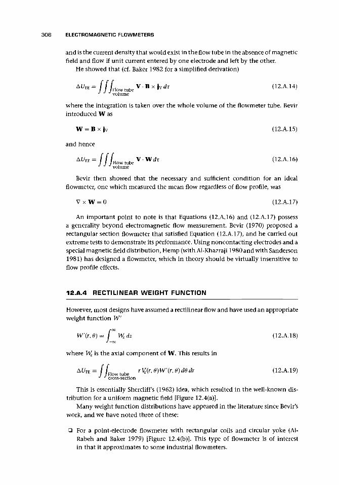
308 ELECTROMAGNETIC FLOWMETERS
and is the current density that would exist in the flow tube in the absence of magneticfield and flow if unit current entered by one electrode and left by the other.
He showed that (cf. Baker 1982 for a simplified derivation)
Al/EE= f f L u V-Bxjv^T (12.A.14)LL II /Flowtube ' v '
J J ^ volume
where the integration is taken over the whole volume of the flowmeter tube. Bevirintroduced W as
W = B x j v (12.A.15)
and hence
volume
Bevir then showed that the necessary and sufficient condition for an idealflowmeter, one which measured the mean flow regardless of flow profile, was
V x W = 0 (12.A.17)
An important point to note is that Equations (12.A.16) and (12.A.17) possessa generality beyond electromagnetic flow measurement. Bevir (1970) proposed arectangular section flowmeter that satisfied Equation (12.A.17), and he carried outextreme tests to demonstrate its performance. Using noncontacting electrodes and aspecial magnetic field distribution, Hemp (with Al-Khazraji 1980 and with Sanderson1981) has designed a flowmeter, which in theory should be virtually insensitive toflow profile effects.
12.A.4 RECTILINEAR WEIGHT FUNCTION
However, most designs have assumed a rectilinear flow and have used an appropriateweight function W
Wf(r,0)= / Wzdz (12.A.18)J—oo
where Wz is the axial component of W. This results in
AL/EE = fXlowtube rM(r,0)W'(r,0)d0dr (12.A.19)** ** cross-section
This is essentially Shercliff s (1962) idea, which resulted in the well-known dis-tribution for a uniform magnetic field [Figure 12.4(a)].
Many weight function distributions have appeared in the literature since Bevir;swork, and we have noted three of these:
• For a point-electrode flowmeter with rectangular coils and circular yoke (Al-Rabeh and Baker 1979) [Figure 12.4(b)]. This type of flowmeter is of interestin that it approximates to some industrial flowmeters.

12.A.4 RECTILINEAR WEIGHT FUNCTION 309
• For a point-electrode flowmeter with diamond coils [Figure 12.4(c)] and circularyoke, which approximates to one introduced in the 1960s and claimed to havea reduced sensitivity to flow profile distortion.
• For a large electrode flowmeter with rectangular coils and yoke (Al-Khazraji andBaker 1979), shown diagrammatically in Figure 12.13, for which the weight func-tion is reproduced in Figure 12.4(d).
The improvement obtained in the uniformity of W by use of diamond coilsinstead of rectangular coils is very noticeable, and there is even more improvementby using large electrodes. However, a major disadvantage of these is the change insensitivity resulting from electrode fouling (Al-Khazraji and Baker 1979).
Hemp (1975) attempted to minimize the variation of weight function with thecopper strip pattern in Figure 12.A.l(a). Figure 12.A.l(b) shows the resulting weightfunction distribution, which should be compared with those in Figure 12.4. Theaxisymmetric weight function was approximately constant for about 87% of thepipe falling to zero at the wall (Figure 12.A.2).
(a)
-0-94 n O;843
1-87124
936
Figure 12.A.1. Hemp's (1975) improvedmagnetic field design: (a) Copper strippattern associated with the improvedmagnetic field. The number associatedwith each line is the value of the mag-netic field potential function, and the ar-rows, which are equal in size in eachstrip, show the direction of the current;(b) Weight function diagram for the im-proved magnetic field (refer to the origi-nal paper for further details; reproducedwith permission from the author and IoPpublishing).

310 ELECTROMAGNETIC FLOWMETERS
w"1.2 r
1.1
1.0
0.9
0.8
0.7
0.60.5
SHERCLIFFLARGE ELECTRODE
DIAMOND COILS
HEMP (1975)
RECTANGULARCOILS
r/a1.0
Figure 12.A.2. Axisymmetric weight functions based on Figures 12.4 and12.A.1.
12.A.5 AXISYMMETRIC WEIGHT FUNCTION
In concluding this section on the theory, it is useful to refer briefly to the axisym-metric weight function. This is given by
W"{r)=—\ / Wzdzd0Z7T Jo J_oo
(12.A.20)
Its value for a uniform field is constant and unity. However, for most prac-tical fields, it falls in value at the outside of the tube. This trend is illustratedin Figure 12.A.2, which gives plots for Shercliffs uniform field weight function[Figure 12.4(a)] and by interpolation for the others in Figure 12.4. The signal isgiven by
AUE , = 2TT f rW"<Jo
(r)Vz(r)dr (12.A.21)
Thus as flow profiles change with increasing Reynolds number from being morepeaked in the center of the pipe to more uniform across the pipe, the signal will fallbelow direct proportionality.
12.A.6 PERFORMANCE PREDICTION
Apart from the design problem, but related to it, has been the accuracy with whichperformance could be predicted from theory. This is the problem of dry calibration.Equation (12.A. 12) suggested a very simple prediction for a uniform field flowmeter.However, the precision of such prediction has always been uncertain. Bevir et al.(1981) have described a very elegant piece of work in which magnetic field measure-ments around the tube wall were used to compute the weight function, and verygood agreement was obtained between prediction based on pipe flow profiles and

12.A.7 FURTHER EXTENSIONS TO THE THEORY 311
actual meter response. They concluded that sensitivities would be predicted for mostflowmeters by their procedures with an error of not more than 0.5%.
Al-Rabeh and Baker (1986) have attempted to predict the performance of aflowmeter from its magnet design. However, although good qualitative agreementon distribution of field was obtained, they found a discrepancy between predictedand actual field size. Thus with care, high accuracy prediction of flow signal may beachieved from actual magnetic field distribution.
Others have developed this approach by measuring and/or predicting the fieldat the pipe wall and using this to calculate the weight function.
12.A.7 FURTHER EXTENSIONS TO THE THEORY
The reader who is interested in various extensions of the theory is referred to thefollowing papers by Hemp and co-workers.
Hemp and Wyatt (1981) explored the use of a "worst flow" to compare electro-magnetic flowmeter performance.
Hemp and Versteeg (1986) developed the analysis of the flowmeter performancebased on the magnetic field on the flowmeter surface. This approach wouldallow 'dry calibration' of a meter based on magnetic field measurements on atube next to the inner surface.
Krafft et al. (1996) discussed the use of the transformer effect signal due to bubblesto obtain both bubble velocity and velocity of the continuous phase of a bubblyflow.
Hemp (1991) developed the theory of eddy currents in electromagnetic flowme-ters and suggested a means of self-calibration. Hemp also (1994c) looked aterrors in potential measurement due to nonuniform contact impedance at theelectrodes.

CHAPTER 13
Ultrasonic Flowmeters
13.1 INTRODUCTION
The first proposal for the use of ultrasound for flow measurement, according toThompson (1978), seems to have been in a German patent of 1928. It was not untilafter 1945 that the idea became more widely proposed. But not until the devel-opment of piezoelectric transducers in the past 40 years or so have ultrasonic ap-plications become really attractive. Fischbacker (1959) provided an early review ofultrasonic flowmeters in which, essentially, the transit-time, sing-around, and beamdeflection methods were mentioned. He also referred to phase-difference measure-ment, means of obtaining sound speed from time measurement and impedance, andhow to obtain density. He saw the advantages of off-axis paths.
Sanderson and Hemp's (1981) review is still a useful source of information onthe subject. The ultrasonic flowmeter's attraction as a flow measurement device isits linearity, lack of obstruction to flow, and, in contrast to the magnetic flowmeter,its ability to measure the flow of gases.
In this chapter, we shall consider three main types of ultrasonic flowmeter, andit is important to understand the strengths and weaknesses of each and that theyare very different in performance and application.
The transit-time flowmeter, or time-of-flight flowmeter, is the most accurate ofthe family and is available as a spool piece meter for liquids and gases or as a clamp-ondesign for liquids only. It can also be retrofitted into a pipe. Measurement uncertaintywill be from a fraction of a percent to about 5%. A transducer in direct contact withthe fluid is said to be wetted, as compared to one that is fixed to the outside of thepipe or has a protective layer between it and the fluid. Transducers for gases must bein contact with the gas (i.e., wetted, a rather inappropriate word for this context!).
The doppler meter is a very different device, and it may be unfair to call it aflowmeter. Its performance is very sensitive to installation, and it has been oversoldto such an extent that many people assume that, when an ultrasonic flowmeteris mentioned, it is one of these. Measurement uncertainty is unlikely to be betterthan about ±2%, and at worst it is indeterminate. Having said this, it has a veryimportant niche in some liquid flow applications where there is an adequate secondcomponent to provide reflection of the beam.
The cross-correlation flowmeter should be capable of reasonable precision (be-tween the preceding two devices), requires a disturbed liquid or multiphase flow tooperate satisfactorily, is likely to be much more expensive than either of the othertypes, and is mainly of interest for measurement in multiphase flows.
312

13.1 INTRODUCTION 313
It is not unusual for other meters that have ultrasonic sensing to be referred toas ultrasonic meters. One such meter is the vortex-shedding meter with ultrasonicsensing.
Beyond these, there is the possibility of using the deflection of the beam to mea-sure flow rate, but to my knowledge this has not been done commercially. There isalso the possibility of measuring density and so turning the meter into a mass meter.
It is important not to confuse the transit-time meter with the doppler meter andto appreciate that the transit-time ultrasonic meter is a far more accurate instru-ment than the doppler meter and should be considered seriously in a wide range ofapplications, especially involving nonconducting liquids or gases.
We shall treat each type of ultrasonic flowmeter in turn. All are based on the factthat ultrasound is made up of acoustic waves at frequencies above the audible range.As a form of sound, ultrasound waves travel with the speed of sound relative to themedium and consist of pressure perturbations in gases and liquids. In solids, the con-necting wave can also move as a shear wave, due to the elasticity of the solid in shear.
In Figure 13.1 (a), we note that the ultrasound is carried by the fluid, so that itsspeed is the sum or difference of its own speed c and that of the fluid V. This is thebasis of the transit-time meter, which uses the difference in time of transit in anupstream and a downstream direction. If the sound is crossing the flow, then theapparent speed is obtained from the hypotenuse of the triangle in the third exampleof Figure 13.1 (a).
In flowmeters, the continuous wave [Figure 13.1(b)] is sometimes used. The di-agram shows the main features of the wave pattern, with the wave length and thehigher and lower pressure regions. The frequency f is related to the sound speed cand wavelength k by f = c/k. The intensity of the transmission varies according tothe angle off the perpendicular axis through the transducer. Three patterns are shownin Figure 13.1(c) for three different ratios of the transducer radius a to the wave-length. The higher the frequency and the shorter the wavelength, the more pencil-like the transmitted beam. A narrow beam is preferable to a wide one because it isless likely to cause spurious reflections, and its path will be better defined. For a speedof sound in water of 1414 m/s, a frequency of 400 kHz will result in a wavelengthof about 3.5 mm, whereas 1 MHz will result in 1.4 mm. For a speed of sound in air of343 m/s, a frequency of 40 kHz will result in a wavelength of about 8 mm, whereas100 kHz will result in about 3.4 mm. Thus for air with k = 2a, the diameter of thepiezoelectric crystal to obtain the middle distribution in Figure 13.1(c) at 40 kHz willbe about 8 mm, whereas the crystal diameters for water are likely to be such thatk < a and result in a narrow intense beam.
More commonly the ultrasound is sent in a small burst of waves. Figure 13.1(d)shows an idealized diagram of a short burst of waves transmitted across the flow.
However, the sweeping effect [Figure 13.1(e)] will mean that the direction of thebeam will be a compromise between high and low flow rates to ensure that it arrivesat the receiving transducer. Another feature of the bending of the beam is that thereis a tendency for downstream sound to be reinforced and for upstream sound to bediffused and weakened (cf. Baker 1996, page 2).
When ultrasound crosses an interface between two different fluids or betweena fluid and a solid, there is both transmission and reflection at the interface. Thetransmission will be greater if the density times wave speed of the two materials

314 ULTRASONIC FLOWMETERS
SOUNDc + V
SOUNDc-y
aZ> C K
V
FLOW FLOW FLOW
(a)
V Wave fronts
[It 2a
Transducerradius a
(b)
- Higherpressure
Lowerpressure
(c)
FLOW
(e)Reduced transmission
angle downstreamIncreased transmission
angle upstream
Figure 13.1. (a) Apparent sound speed as viewed by an observer outside the moving medium.(b) Ultrasonic waves move forward with the speed of sound and with a wavelength X from asource, (c) Radiated intensity variation with angle from a piston transducer set in a plane wall(after Morse and Ingard 1968). (d) Wave packet, (e) Ultrasound waves (like sound waves) canbe bent by the flow and reinforced or dispersed.

13.2 TRANSIT-TIME FLOWMETERS 315
are similar in size. Thus, it proves difficult to transmit ultrasound from air, throughmetal, and then into a transducer. On the other hand, it is possible to transmit fromliquid through a solid and then to a transducer. The relevant characteristic of thematerials is the impedance.
Impedance = Density of material through whichultrasound is transmitted x Velocity ofultrasound in the material
Z = p x c (13.1)
and using approximate values at 20° C for air
Z = 1.19 x 343 = 408 k g n r V 1
for water
Z = 1000 x 1414 = 1.41 x 10⁶ k g n r V 1
and for steel
Z = 8000 x 5625 = 45 x 106 kgm~V1
The proportion of ultrasound power transmitted is given by Asher (1983; cf.Asher 1997) as
2(13.2)(Zi + z2y
and that reflected is
Thus whereas transmission from steel to water is about 12%, that from air to steelis negligible. In discussion at a symposium on flow measurement (Trans. Soc. Instrum.Eng., Vol. 11, June 1959), Bertele of ICI raised the problem of getting enough energyinto the gas. As a result, we shall find that transducers for gas flow measurementmust be wetted.
The final point to make is that attenuation increases with increasing frequencyand tends to be greater in gas than in liquid.
13.2 TRANSIT-TIME FLOWMETERS
In this section, the operation is described, and the key flowmeter equations are given.The simple theory of these devices is given in Appendix 13.A.1-13.A.3, with a briefreference to some fuller solutions.
13.2.1 SIMPLE EXPLANATIONThe transit-time flowmeter depends on the slight difference in time taken for an ul-trasound wave to travel upstream rather than downstream. Thus waves are launched

316 ULTRASONIC FLOWMETERS
Figure 13.2. Geometry of the transit-time flowmeter.
each way, their time of transit is measured, and the difference can be related to thespeed of the flow. Apart from the smallest bore flowmeters, it is usual to send thebeam across the flow but not at right angles to the flow, so that there is a compo-nent of the fluid velocity along the path of the acoustic beam. Figure 13.2 is a simplediagram of an ultrasonic flowmeter geometry.
13.2 .2 FLOWMETER EQUATION AND THE MEASUREMENTOF SOUND SPEED
We can show that for a uniform velocity in the pipe (Appendix 13.A.1), we canobtain an expression in terms of the transit times of upstream tu and downstream ^wave pulses, and the time difference At:
L2AtV = (13.4)
where L is the path length, and X is the axial spacing between transducers. This isone form of the equation, and others are set out in Appendix 13.A.1.
The reason for the product tutd in Equation (13.4) is to eliminate the speed ofsound, which otherwise appears in the equation. By measuring the mean time oftransit, and VMi approximates to this, and by knowing the transit distance, we canobtain the speed of sound.
In the transit-time method, pulses of sound of a few cycles in length are trans-mitted in each direction (Figure 13.3), and the time taken for them to reach thereceiving transducer is measured. Hemp (1982) gave examples of pulses:
Water metering:
Domestic gas:
50 mm diameter pipePulse of 6 cycles1-MHz carrier1.5-mm wavelengthWave packet about 9 mm long12-mm diameter pipePulse about 13 cycles2-mm wavelengthWavepacket about 26 mm long

13 .2 TRANSIT-TIME FLOWMETERS 317
Downstreampulse
Figure 13.3. Diagram to explain transit-time measurement.
Upstreampulse
We obtain from Equation (13.4), assuming V is constant across the pipe,
_ nD2V4
7tD2L2At(13.5)
It is important to appreciate the value of the times involved in these measure-ments. If the flowmeter is to discriminate to better than 1%, we may define E(Af)as At/100, and for two meters, we obtain the values in Table 13.1 (Baker 1988/9).
Table 13.1 highlights the problem of the very small time differences we need tomeasure in the transit-time flowmeter. For the smaller tube, this is to better than1 ns. However, one advantage of this system is that any echoes or standing waveshave time to die down, another advantage is that the same path can be used for eachdirection of the pulse, and, finally, the individual measurements can be used as atolerance check to ensure that spurious measurements are rejected (Scott 1984).
An alternative way to eliminate sound speed is the sing-around method(Figure 13.4) discussed by Suzuki et al. (1975, cf. 1972). In this method, each ofthe paths, upstream and downstream, is operated in such a way that when the pulseis received by the receiving transducer, it triggers a new pulse from the transmittingtransducer. Thus the frequency of pulses is dependent on the velocity of sound and
Table 13.1.
Diameter(mm)
100300
Transit-time meter times
(*U + <d)/2 (s) At(s)
io-4 io-7
3 x 10~4 3 x IO-7
E(At) (s)
io-9
3 x IO-9
6 = 45°, V = 1 m/s, and c is taken as 1430 m/s, the valuefor water at 4°C.

318 ULTRASONIC FLOWMETERS
of the flow. We find that the frequency ofpulses is given by
= 2XV/L2 (13.6)
which has the virtue of relating V to thefrequency difference without requiring thevalue of c, the sound speed. Again we canobtain typical values for the frequenciesfrom Table 13.2 (Baker 1988/9). Making theapproximation that V is constant across thepipe, we obtain
nD2L2AfSX
(13.7)
Figure 13.4. Diagram to explain sing-around system.
The limitation of the sing-aroundmethod relates more to the very low fre-quencies and the long time periods neededto achieve sufficient accuracy. To achieve
1% uncertainty, we shall need to have a measuring period of greater than 1 s for themost favorable of the cases in Table 13.2.
Timing can also be achieved in some cases by obtaining the phase shift betweenthe two arriving waves to obtain the time difference (Baker and Thompson 1975).Other problems such as standing waves and spurious transmission paths that cannotbe gated out may need to be considered in relation to any of the methods chosen.Unwanted reflections within the pipe and their effect on the measurement uncer-tainty may be reduced by the use of higher frequencies. These attenuate reflections,but they also attenuate the signal. Cunningham and Astami (1993) produced curvesof upper and lower frequency limits against pipe diameter for various reflection set-tling times. The upper limit ensures that signal attenuation is not too great, whereasthe lower limit is to ensure that attenuation of reflections is sufficient. They reckonedthat the received signal should be at least 30% of that transmitted.
An alternative approach, rather than measuring the value of c, is to use thefact that c2 = l/(ksp) for a particular liquid and that c2 = yp/p for a particular gas[Equation (13.A.3)]. For a liquid,
2ksXpVSksXqm
7ZD2 (13.8)
Table 13.2. Sing-around meter frequencies
Diameter V=lm/s V=10m/s(mm)
100300
e = 45°,water at
V =4°C.
fd10,
3,
1 m/s
(Hz)
117372
, and
Af (Hz)
103.3
cis taken as 1,430
fu (Hz)
10,1623,387
m/s, the value
10033
for
(Hz)

13.2 TRANSIT-TIME FLOWMETERS 319
Table 13.3. y for various gases from Haywood (1968)
Type of Gas Mean(number Examples Value Valueof atoms) of Gases of 7 of7fl
11!
I|t11Iv!t*
MonatomicDiatomic
3-5 atoms3 atoms5 atoms
8-9 atoms8 atoms9 atoms
ArgonAirNitrogenOxygen
Carbon dioxideMethane
EthanePropylene
a Based on number of atoms.
1.671.401.401.40
1.311.31
1.191.15
1.671.40
1.29
1.17
where the adiabatic compressibility would need to be known and, because it varieswith temperature, would need to include some temperature compensation. For a gas,
A ^ 2pXVyp
$Xqm
nD2yp (13.9)
thus relating the mass flow rate of a gas to the time difference, the pressure of thegas, and the geometry of the flow tube. Table 13.3 gives values of y, and a flowmeterusing this method would need a selection switch for the type of gas in addition tothe pressure measurement facility.
An alternative method to obtain the mass flow is to obtain the density fromthe value of the impedance discussed earlier. Guilbert and Sanderson (1996a) havedescribed such an ultrasonic mass flowmeter, which combines a fairly standardconfiguration of ultrasonic flowmeter with an impedance density cell, in whichthe impedance of the liquid is obtained through the interface between the liq-uid and a material that divides the cell into compartments. The material selectedwas polyamide/imide. They also used the time between reflected signals to ob-tain the sound speed in the divider and hence its impedance (cf. Chapman andEtheridge (1993) who described the evolution of the ultrasonic flowmeters for gasmeasurement).
13.2 .3 EFFECT OF FLOW PROFILE AND USE OF MULTIPLE PATHS
The preceding simple analysis has assumed that the flow profile is uniform. In fact, ifwe allow for varying velocity along the path of the ultrasonic beam, Equation (13.4)may be rewritten in the form
L2At2Xtutd
(13.10)

3 2 0 ULTRASONIC FLOWMETERS
Figure 13.5. Acoustic beam positions (T, top of pipe, indicates possible preferred orientation inliquid flow): (a) Diametral path; (b) Mid radius paths; (c) Four path; (d) Reflex mode with Wpath; (e) Reflex mode with two V paths; (f) Reflex mode with triangular path.
where Vm is the mean velocity along the path of the beam, since the flowmeter aver-ages velocity along the path of the beam. In general, this average does not correspondto the area average of the velocity required for an ideal flowmeter. Unfortunately, forcircular pipes with paths crossing the diameter [Figure 13.5(a)], the mean velocityalong the path gives too heavy an emphasis to the flow at the center of the pipe. Thisimplies that change of profile from laminar to turbulent and through the turbulentrange will affect the calibration. It is easy to show (Kritz 1955) that the effect ofintegrating a laminar profile across a diameter of the pipe causes a signal about 33%high due to the overweighting that the velocities near the axis receive, comparedwith a uniform profile. Through the turbulent range, using the 1/n power law (seeChapter 2) for a Re number variation between 103 and 106, a variation of about3% occurs. Apart from Kritz, others have provided calibration factors (Kivilis andReshetnikov 1965, Del Grosso and Spurlock 1957). Thus for a meter that is con-structed this way, there is an inherent variation in calibration factor, which cannotbe wholly allowed for in the transmitter circuitry due to Reynolds number depen-dence on factors other than velocity only. Scott (1984) made the point that a changein viscosity from 1 to 10 cP causes a change in profile, which will account for a 1%error.
One way to improve this is to offset the paths from the axis [Figure 13.5(b)], inwhich case a position at about the mid radius is found to be a good compromise(Appendix 13.A.2). Baker and Thompson (1975) showed the effect of offset paths(Figure 13.6) for varying Reynolds number on the signal with the paths offset at0.5R, 0.505R, and 0.523R from the axis. This shows that a position of 0.523R is idealfor the turbulent range, whereas 0.505R is probably a reasonable compromise for

13.2 TRANSIT-TIME FLOWMETERS 321
% error
Figure 13.6. Calculated values of the percentage error against Reynolds number for three posi-tions of the acoustic paths (after Baker and Thompson 1975).
the whole Reynolds number range. They also suggested that the meter should havelow sensitivity to swirl and to flows that have symmetry of size but opposite senseabout the axis.
Hastings (1968, 1970) used four paths [Figure 13.5(c)] and selected their posi-tions so that a Gaussian Quadrature integration (a numerical method for integrat-ing general curves, which is similar but more complicated than Simpson's rule - seeAppendix 13.A.2) could be used to give a correct mean velocity signal for profilesthat are formed from polynomials of seventh power or less. Again the experimentalevidence since these early papers confirms the quality of the integration achievedand the potential accuracy of the design.
Using the velocity measured on multiple paths, Vaterlaus (1995) gave the fol-lowing positions for multiple paths and the weight to be given to each:
Planes
2
3
4
Distance fromcenter plane
±0.5200
±0.774±0.339±0.861
Weight
0.5
0.4440.2770.3260.174
The value given for two paths agrees well with Baker and Thompson (1975).Taylor and Cassidy (1994) quoted weightings for four planes, which, to three signif-icant figures, agreed with these (cf. Pannell et al. 1990 on a generalized approach topositioning chordal paths).

322 ULTRASONIC FLOWMETERS
A variation on the positioning of the paths uses internal reflection of the beams toallow transmitter and receiver to be on the same side of the pipe [Figures 13.5(d, e)].This is known as reflex mode. This can be either V with one reflection or W withthree reflections. It can also be used to create subtle reflections, which essentially givethe path position the benefits of off-axis integration [Figure 13.5(f)] and multiplepaths around the pipe to give even better integration of the profile. An exampleof this results in the paths lying on an equilateral triangle if viewed axially downthe pipe, thus using the midradius point but also covering a large area of the tube(Drenthan and Huijsmans 1993).
Jackson et al. (1989) developed an ultrasonic flowmeter using one transmittingtransducer and a lens system made of Perspex, which produced a diverging ultra-sound beam detected by three widely spaced receiving transducers. The chords of thethree paths are all designed to be of different lengths and angles. In the test meter, afurther path was used across the flow to obtain the sound speed. It is not obvious thatthis design contributes significantly to the normal design with three complete pathsor, indeed, the designs using reflecting beams to obtain off-diametral paths. The ad-vantage of reciprocating paths is that the sound speed is obtained using the mean.
Jackson et al. (1991, cf. 1989) described a three-path meter where the path an-gles were chosen to obtain information about the flow profile. The paths were in adiametral plane and with chordal paths on each side at angles of 44° and 52° to thediametral plane. For axisymmetric profiles, performance was of order 2%. Asymme-try was detected unless there was a symmetry about the diametral plane, but preciseflow measurement with asymmetry was not obtained.
Van Dellen (1991) of Daniel Industries, Inc., demonstrated compensation byusing multiple paths. Such designs allow self-checking routines where speed of soundis compared and successive measurements can be used.
Multipath meters are an option for hydroelectric turbine efficiency measure-ment. Lowell and Walsh (1991) reported on the use of eight eight-path crossed planemeters and concluded that ±0.5% uncertainty of flow rate could be achieved withappropriate relative positioning of acoustic plane and upstream fittings.
Sanderson and Hemp (1981) also mention the use of a wide beam to average theflow rate.
Hemp (1982) has developed the concept of weight vectors (cf. Appendix 13.A.3)and in a more recent paper (Hemp 1997) showed a weight function distribution forpoint transducers (which, in practice, would presumably need to be small area) ina circular pipe. This indicated that the meter was most sensitive to flow near thetransducers.
See Smith and Morfey 1997 on the effect of beam bending due to velocity vari-ation across the pipe.
13.3 TRANSDUCERS
One of the most important features of the mechanical design of the meter is thetransducer and its mounting. This must achieve
• efficient transmission and reception of acoustic signals through the interface,

13.3 TRANSDUCERS 323
• negligible acoustic transmission through the body of the flowmeter,• accurate and permanent positioning,• no adverse effects due to operating fluid, and• trouble-free performance.
Transducers fall into a number of categories, and these will be worth bearing inmind in the following discussion:
Factory installed Wetted transducers - open cavityNonwetted transducers - open cavityNonwetted transducers - filled cavity
Note: For any of these, the spool piece may be factory wet calibrated. Only thefirst is suitable for gases.
Retrofit Wetted transducers - open cavityNonwetted transducers - open cavity
Note: Only in situ calibration is possible. Dry calibration by very carefulmeasurement may be acceptable.
Clamp-on Nonwetted transducers - transmission through pipe wallNote: Wet calibration is virtually impossible. This transducer is not suitablefor gases.
Figure 13.7 shows some typical mounts for transducers. Figure 13.7(a) shows awetted transducer in an angled mounting block. The crystal emits a pencil of soundthrough perpendicular interfaces, and it is not therefore refracted. Figure 13.7(b)shows an alternative arrangement with mounts perpendicular to the tube and trans-ducer with an angled end in which the crystal is mounted. If the liquid is aggressiveor particle laden, some form of window may be required. In this case, the transducermay be mounted as shown in Figure 13.7(c), where a metal window is used butwhere all interfaces remain perpendicular to the beam. The cavity is a source of flowdisturbance and solid deposit. Both may cause signal failure or flow measurementerrors. Figure 13.7(d) has the cavity smoothed off with a filler of some sort such asan epoxy. Ideally, this filler should have an acoustic refractive index similar to theliquid, thus keeping refraction to a very low value, and the bending of the acousticray on crossing the interface will be small. However, changes of fluid or tempera-ture may introduce errors. An important advantage of the mounts shown in Figures13.7(a, b) is that alternative transmission around the tube wall and outside the fluidis reduced, and in practice the transducer mount can be made to absorb it. Withthe mounting systems in Figures 13.7(c, d), the signal processing must discriminatebetween the fluid-borne signal and the spurious signals around the wall of the tube.Sanderson and Hemp (1981) gave some details of ways to increase the bandwidth ofthe piezoelectric plate.
Figure 13.7(e) shows a clamp-on system in which the transducer mount is entirelyexternal to the tube and may be mounted on existing tube. Here the problems ofthe type found in the mounts shown in Figures 13.7(c, d) are greatly increased.
For very small pipe sizes, the limitations of pipe diameter and consequent shortpulse times can be overcome by a flow tube and transducer mounting system of the

324 ULTRASONIC FLOWMETERS
1/(b)
(d)
(e)
Figure 13.7. Transducer mounts (cf. Baker 1988/9): (a) In line - wetted; (b) Angled - wetted;(c) In line - window protection; (d) In line but with cavity filled with epoxy or other filler;(e) Clamp-on transducer with crystal embedded in the mount; (f) In-line transmission for smalltubes with either wetted or protected transducers.
type shown in Figure 13.7(f). The flow enters a section of tube in which the acousticbeam is axial, and hence there is no limitation on the separation of transducers apartfrom those resulting from the application.
For gases, it is essential that the transducers are in contact with the fluid and soare mounted as shown in Figures 13.7(a, b) or possibly Figure 13.7(f).

13.5 SIGNAL PROCESSING AND TRANSMISSION 325
To overcome the impedance mismatch, a low impedance transducer was re-ported (Collings et al. 1993). When used in a meter, it allowed natural gas flowsof 0.013-8 m3/h with a temperature range of —13 to 47°C and is claimed to havesignificant advantages over current domestic meters.
It should also be remembered that for high pressure service the transducers mustbe flanged to the correct line pressure (rather than screwed). Transducers that projectinto the tube may avoid attenuation and other problems due to air collection withinthe pockets. To reduce turbulence caused by the transducer cavities on a 20-mm-IDultrasonic flowmeter for gas, nets have been placed to create a wall that transmittedthe ultrasound (Hakansson and Delsing 1992).
Lynnworth (1988) suggested the use of new types of wetted and clamp-on bufferrods to allow for extreme temperature (e.g., ±200°C) such as might occur in wetteduse in cryogenics or in the flow of quench oil in a carbon steel pipe at 260°C.
13.4 SIZE RANGES AND LIMITATIONS
Single- and twin-path designs may be available for liquids in 80-2,000 mm diameteror greater, although very large sizes may be retrofit applications. The arrangementfor small tubes is likely to be for 10-80 mm.
When retrofitting, there is always a tolerance on the pipe dimensions, both di-ameter and wall thickness, which will affect the deduction of mean flow from ul-trasound path velocity, and the measurement needs to take account of the actualseparation of transducers (Scott 1984). For instance, in a carbon steel pipe with a100-1,000 mm diameter, the tolerance may be ±1% on diameter and ±10% on wallthicknesses of 3-5 mm. In addition, erosion, corrosion, and painting of the pipemakes it improbable that the error can be reduced below 0.5%. Manufacturers mayoffer retrofit for one, two, or four paths, which with precise internal measurementshould be capable of high accuracy.
13.5 SIGNAL PROCESSING AND TRANSMISSION
As indicated earlier, the measurement system essentially requires the ability to mea-sure very small time periods, or periods to very high precision. This increment couldbe of order 10~9 (a nanosecond), which Sanderson and Hemp (1981) pointed outwas comparable with the (then) propagation delays and rise times of the fastestcommercially available logic. Clearly the technology in this area is moving rapidly,and the problems encountered in small time measurement, phase comparison, orsing-around are finding new solutions.
Tables 13.1 and 13.2 have identified the design requirements for the signal pro-cessing, namely,
• for transit-time meters to measure timed differences to better than 10~9 s (onenanosecond) and
• for sing-around meters to measure frequency differences to better than, say,0.03 Hz for 1% discrimination in a 300-mm tube with V = 1 m/s.

326 ULTRASONIC FLOWMETERS
To achieve this, various clock circuits have been used. In an early commercialmeter, a ramped voltage system provided a time measure. In addition, there areproblems in ensuring that the zero-pass, or whatever part of the wave is used, isconsistent between transmitters and receivers. Szebeszcyk (1994) discussed someaspects of the design of the ultrasonic flowmeter and transducers, use of first zerocrossing of the signal, optimum thickness of matching layers, etc.
Vaterlaus (1995) described a time measurement system with two counters. Onecounter Nt was clocked during the measuring period by a stable quartz oscillator witha frequency f — 64 MHz, whereas the other counted the number of samples Nn. Astart pulse initiated the measurement by activating the two counters and triggeringthe ultrasonic pulse emission. During the measurement period r = 30 ms, everypulse received caused a new pulse to be emitted. The two counts Nt and Nn wereused to calculate the propagation time from Nt/Nn.
It appeared that x was obtained precisely from Nt/f; hence, provided x endedafter a complete value of Nn, it was possible to obtain the transit time as Nt/(Nn f)and a resolution of 60 ps in 116 /xs was claimed.
Advantages claimed were:
• Velocity resolution was to 0.8 mm/s.• Precision depended on the stability of the oscillator.• Jitter in digital logic was averaged.
Another solution to the timing problem (Pavlovic et al. 1997) appeared to use
a. a transmitted pulse in two halves, the first at one amplitude and the second attwice the amplitude, presumably allowing more precise timing edges;
b. the downstream and upstream times were then given by
t& = NdT+ Ard
ta = NUT + Aru
where Nd and Nu were the whole number of counter periods of a 2.2-MHz squarewave train obtained from a 17.7-MHz oscillator through a divider by 8 and wereobtained by standard counter methods;
c. Ard and Aru were measured through the phase difference between transmissionand received signals, and a two-stage measurement system using a coarse andfine approach. An integrator was used to obtain Aid and Aru.
The effects of error due to temperature on pipe diameter, recesses, delays inelectronics, and transducers were also addressed.
Because such short times are being measured, system designs need to address de-lays in the cables, transducers, and converter (Scott 1984). Time delays of microsec-onds could lead to errors if the head is calibrated on water for use on oil (±1.5%), orif the temperature of the water changes by 10°C (±0.1%). Further delays are causedin the window, or in the transmission through the wall, ranging from about 3 /is toabout 15 /xs. These delays will also be dependent on the choice of materials.
Hemp (1988, 1998) has proposed a reciprocity approach to the elimination ofzero instability. This requires that the transducers are driven, say, by a voltage pulse,

13.6 ACCURACY 327
and that the received signal is then sensed by its current pulse. The path is thenreversed.
13.6 ACCURACY
Van Dellen (1991) suggested that the ultrasonic meter could meet custody transferaccuracies, and this appears to be happening (cf. Selvikvag 1997).
Reports indicate that good accuracy can be achieved by dry calibration - theuse of flowmeter dimensions to obtain calibration (de Boer and Lansing 1997).Zanker and Freund (1996) even suggest that the difficulties of calibrating a large(30-in. or 75O-mm)-diameter meter may make dry calibration preferable. This will,in part, reflect the limitations in the flow calibration facilities at large volume flowrates.
13.6.1 REPORTED ACCURACY - LIQUIDS
Cascetta (1994) compared a clamp-on transit-time ultrasonic meter with an elec-tromagnetic meter in situ in a water distribution network with 400 mm ID. Theultrasonic meter generally overestimated the flow rate, and the difference betweenthe ultrasonic and electromagnetic flowmeter was mainly in the range ±1-5%.
Delsing (1991) tested the zero-flow performance of a sing-around ultrasonicflowmeter with multiple paths. The meter was in a 25-mm line, with transducersset at 20° to the flow direction, and of 15 mm diameter. The sound path was 96 mm,giving a period of about 64 /xs for a sound speed of 1,500 m/s. The single-period reso-lution was about 15 ns, giving a velocity resolution of about 0.18 m/s. This could beincreased by using multiple-period averaging techniques. For instance, using 1,000sing-around loops, a theoretical period measurement resolution of about 15 ps andvelocity resolution of about 0.18 mm/s could allow measurement down to 1.8 cm/swith an uncertainty of ±0.5%. The experimental data showed an overall zero-flowerror of less than ±0.6 mm/s, which would allow uncertainty of ±1% for flows aslow as 6 cm/s, and Delsing suggested that this would open up the meter's range to100:1.
Manufacturers of commercial meters tested at NEL (Brown 1996) seemed to claimfor uncertainty, in the main, about ±0.5% of rate, but there appeared to be quite alot of variation in actual performance between designs.
13.6.2 REPORTED ACCURACY - GASES
Holden and Peters (1991) found that, for undisturbed flow, the British Gas 300-mmmeter readings lay within 0.4 and -0.8% of the reference turbine meters. For a150-mm meter, the variation was between 1.4 and -0.35%, and a 500-mm meterappeared to be within about 0.3%.
A 6-in. (150-mm) ultrasonic meter calibration against sonic nozzles (with repeata-bility of 0.04%, Erdal and Cabrol 1991) gave a day-to-day repeatability of 0.1%.
Grimley (1996) tested Daniel and Instromet meters and concluded that they werecapable of accuracies within 1% tolerance and with repeatability better than 0.25%.Pressure change (e.g., 4.5 MPa) caused shifts of 0.4%. It also suggests that, for drycalibration, there will be a need to understand the effect of parameter changes.

328 ULTRASONIC FLOWMETERS
13.6.3 MANUFACTURERS' ACCURACY CLAIMSTypical performance claims for single-path meters for liquids with wetted transducersare ±1% of full scale. Repeatability of ±0.2% full scale may be available. Abilityto cope with entrained solids or gas bubbles is increasing. Wetted transducers areavailable for temperature ranges from —200 to +260° C and pressures up to 200 bar.Pipe sizes range from less than 50 mm to 2 m. Fluid velocity in the pipe can rangefrom 0.03 to 10 m/s or higher.
For gases, the accuracy is likely to be of order ±0.5-5% of reading, and repeatabil-ity will range from 0.25 to 0.5% of reading, with a range of velocity of 0.3-45 m/s.Duct sizes can range up to 10 m. Temperature range may be as much as -50 to+260°C.
13.6.4 SPECIAL CONSIDERATIONS FOR CLAMP-ON TRANSDUCERSFor clamp-on meters, manufacturers appear to be unwilling to claim better thanabout 3% of rate at higher flow rates, or even 3% of full-scale deflection for lowflow rates. However, as in at least one case, the manufacturer may give figuressuch as
• repeatability if nothing changed, ±1%;• uncertainty (D < 25 mm), ±10%;• uncertainty (25 < D < 50 mm), ±5%; and• uncertainty (D > 50 mm), ±3%.
Sanderson and Torley (1985) described an intelligent clamp-on flowmeter andclaimed an uncertainty within ±2% of reading. They concluded that the wedge an-gle of the transducers (estimated uncertainty of ±1°) could account for much of theerror. They gave plots of baseline drift equivalent to about 30 mm/s. They demon-strated the value of Hemp's (1979) reciprocal drive system on baseline stability (e.g.,where there is temperature change), which reduced drift to about one-eighth of thatfor a conventional system. They found that an error of ±2.5% in transducer separa-tion resulted in errors within 0.5%. The meter used additional transducers to locateoptimal axial separation of transducers and for self-calibration. The transducers al-lowed pipe wall thickness to be measured and also internal dimensions of the pipe.They also gave a very useful analysis of the likely errors in the system.
Cairney's (1991) experience of dedicated transducers, where there is a specificpair of clamp-on transducers for each different size of pipe, with a scale card withinthe portable electronics unit, was that, within the limitations, accuracy and repeata-bility were good for pipes with OD greater than 35 mm. An example is the measure-ment of lubricating-oil flows at near ambient temperature in a 60.4-mm OD linewith 5.5-mm carbon steel wall. Reynolds number was 50-350 (laminar). Readingswere within ±3% of a volumetric tank, where ±3% was typical above 35 mm OD,but below this errors tended to increase. It seems that Cairney also implied thatremoving and replacing the transducers led to larger errors, typically in the range5-10%.
Cairney's (1991) experience of multipurpose transducers, which allowed the useof one pair of transducers for a wide range of pipe sizes, was that the unit wouldoperate with almost any homogeneous, Newtonian liquid and on any pipe that

13.6 ACCURACY 329
Table 13.4. Pipe material and sizes used by Cairney (1991)
Materials
Carbon steel
Stainless steelAluminumUnplasticized
polyvinyl chloride (UPVC)
Outside Diameter(mm)
60.4-61.089.133.3-33.733.4 & 33.563.733.5 &33.7114.3
Wall Thicknesses(mm)
5.55-8.66.53.89-6.211.74 & 2.866.65.10 & 2.395.4
conducts sound. Relevant details are fed into the electronics unit: pipe geometry,material, and fluid properties. The manufacturer claimed ±3% uncertainty withoutcalibration. Cairney tested the meters to check this claim. The tests were all in hori-zontal pipes with the transducers mounted on the horizontal centerline. Pipe detailsfor his tests are given in Table 13.4.
For most of the tests flowmeter uncertainty was within ±5%. Particular notesfollow:
• Flow rate and pipe material had no noticeable effect, and coupling to the pipewas not a problem.
• Performance was similar in direct and reflex modes.• Rust on the inner surface is more likely to affect the cross-sectional area of the
pipe than the signal transmission.• The ratio of pipe diameter D and wall thickness t should be greater than 15;
D/t > 10 is acceptable, and D/t < 10 may cause problems due to ultrasoundtransmission around the pipe wall. The low values may increase the uncertaintyto order ±10%.
• Removal and replacement of transducers caused, on some occasions, a severeshift in reading traced to an incorrect measure of sound speed. This appeared to bea fault with the electronics. Cairney recommended checking the computed speedof sound. Provided care is taken, the removal and replacement of transducersshould contribute only about ±2% to the error.
• Air bubbles can cause loss of signal strength, which should, therefore, be moni-tored.
• Nominal pipe dimensions should not be used. A 1-mm error in a pipe of 50-mmdiameter results in about 8% error in cross-sectional area.
• Incorrect axial spacing of the mounting tracks is not significant, but incorrectangular spacing can cause errors up to ±10%.
Cairney concluded that errors should be containable within about ±5%.Commercial devices allow a range of materials for the pipe including steel, stain-
less steel, cast iron, vinyl chloride, fiber reinforced plastic (FRP), and asbestos, insizes from 6 mm or less to 9,000 mm. The presence of a lining of tar, epoxy, mortar,or Teflon appears to be surmountable. They may be available in both reflex (one ormore internal reflections off the pipe wall) or direct mode.

330 ULTRASONIC FLOWMETERS
Sensitivity as small as 0.3 mm/s and zero drift of 3-6 mm/s has been suggestedwith uncertainty claims of 1.5% reading down to 1 m/s. The meter should be capableof measuring flows in continuous liquids with low attenuation of the beam and noair bubbles, etc.
NEL (1997) reckoned that, with care, clamp-on meters could achieve spool pieceprecision, but diametral paths were a limitation. An error in the measurement ofdiameter of, say, 1% would result in a cross-sectional error of 2%. However, the pointwas also made that temperature change could lead to changes in the refraction angle.
13.7 INSTALLATION EFFECTS
In addition to the following effects, it should be remembered that with these pre-cision instruments, in which the accuracy of mounting transducers and generaldimensional stability is important, temperature variation within the measuring re-gion of the flow tube, stresses in pipe fixtures, unsuitable mounting, and even JoeBloggs who regularly taps the pipe with his spanner as he walks by or climbs on itas a step, may have detrimental effects on precision.
Zanker and Freund (1994) found that less than 1% condensate had little effect(+1%) and that the meter survived in site trials, despite adverse conditions. NEL(1997) reckoned that the maximum air-in-water for satisfactory operation was 0.5%by volume, but that oil-in-water was a lesser problem.
Heritage (1989) reported an important series of tests on the performance oftransit-time ultrasonic flowmeters using water as the test fluid. The first part of herwork indicated the surprisingly large failure rate of new flowmeters. Out of 11 dif-ferent flowmeters from seven manufacturers, 3 failed to complete the test program,only 2 performed within the manufacturer's specification, and differences of as muchas 1.7% of rate were observed between the analogue and pulse outputs for certainmeters. Based on analogue readings, 2 meters were within 2%, 3 were within therange 2-5%, 2 were within the range 5-10%, and 2 were over 10%.
13.7 .1 EFFECTS OF DISTORTED PROFILE BY UPSTREAM FITTINGS
Some early reported installation effects (Al-Khazraji et al. 1978) obtained by com-bining measured flow data for an eccentric orifice discharge at 5.5D with theoreticalcalculations suggested that a single-path meter could have errors of 5-16%; a twinpath meter, ±1.6%; and a four-path meter could have errors of less than 1%.
Tables 13.5-13.7 summarize the installation tests of Heritage (1989) on water. Inthe original paper, the results of two single-path meters are reported separately, butthey are combined in Table 13.5. The effect of the gate valve is taken regardless oforientation. This is partly because the differences did not appear to be substantial,and the safe assumption is the range given. The same is true for the two bends,which were in perpendicular planes. However, in this case, the variation betweenthe meters is so great that it appears to outweigh any effect of orientation.
It appears from Tables 13.5 and 13.6 that a single-path meter will probably re-quire at least the spacing for 0.75 beta ratio orifice. For dual-path flowmeters, theperformance (Table 13.7) appears to be close to that for an orifice with p = 0.6 with±0.5% additional uncertainty.

13.7 INSTALLATION EFFECTS 331
Table 13.5. Installation tests on water for single-path meter(after Heritage 1989)
Spacing Between Downstream Flange ofDisturbance and Upstream Flange of Meter
(Error Range in Percentages)Disturbance 5D 10D 15D
Gate valve50% closedby movement
Swept bend(r/d= 1.5)parallel
Swept bend[r/d= 1.5)perpendicular
Two sweptbends
Reducer
Not obtained - 1 to -2.5 +1.5 to -3
Not obtained +4.5 to -6.5 -2 to -3.5
Not obtained -3.5 to -4.5 +3.5 to -3
Not obtained +7.5 to -11 -0.5 to -7
Not obtained +2 to -4.5 +2 to -1
Halttunen (1990) used data on flow profiles and applied them to the ultrasonicflowmeter analyses to obtain the effect of flow distortion on the performance. Healso gave experimental data from installation tests presumably on water. Each of hismethods appeared to give a slightly different datum, a salutary reminder that all suchmeasurements and predictions are subject to some uncertainty. The conclusions thatcan be drawn from the plots are given in Table 13.8.
Table 13.6. Installation tests on water for single-pathclamp-on meter (after Heritage 1989)
Spacing Between Downstream Flange ofDisturbance and Upstream Flange of Meter
(Error Range in Percentages)Disturbance 5D 10D 15D
Gate valve Not obtained +3 to -2.5 +1.5 to -0.550% closedby movement
Swept bend Not obtained +3.5 to -3 -2.5 to -3.5[r/d= 1.5)parallel
Swept bend Not obtained -2 to -2.5 +2.5 to -3.5[r/d= 1.5)perpendicular
Two swept Not obtained -5 to -10 +0.5 to -6bends
Reducer Not obtained -2.5 to -4.5 0 to -0.5

332 ULTRASONIC FLOWMETERS
Table 13.7. Installation tests on water for dual-path meter(after Heritage 1989)
Spacing Between Downstream Flange ofDisturbance and Upstream Flange of Meter
(Error Range in Percentages)Disturbance 5D 10D 15D
Gate valve50% closedby movement
Swept bend(r/d= 1.5)parallel
Swept bend(r/c?= 1.5)perpendicular
Two sweptbends
Reducer
0 to+1.5
Oto +1
+0.75
-1 .5 to - 3
+1 to +0.5
+0.75
+0.25
-0.75
Not obtained
Not obtained
Not obtained
+0.5 to -1.5 Not obtained
+1 to +0.5 Not obtained
The orientation for single-path ultrasonic flowmeters may cause an additional±1% at 10D or less spacing, and for dual-path ultrasonic flowmeters it may cause anadditional ±0.5% at 5D or less spacing.
The following claims of Vaterlaus (1995) appear, possibly, optimistic but probablyreflect the (surprising) variation found by Heritage (1989). For a single-path meter,errors should be within 1% if at least:
10D is allowed between a reducer and the meter;20D is allowed for an elbow or a T;25 D is allowed for two elbows in one plane;40D is allowed for two elbows in perpendicular planes; and50D is allowed for a partially open valve or for a pump.
Table 13.8. Halttunen's (1990) installation data5D 10D 20D 40D 80D
Ultrasonic flowmeter — single pathSingle elbowDouble elbow
90°
- 5 %- 7 %
-2 .5%- 5 %
Ultrasonic flowmeter — dual pathSingle elbowDouble elbow
90°
- 1 %±1.5%
-0 .5%±1%
- 2 %- 3 %
small±1%
—- 1 %
—+0.5%
- 1 %
+0.5%

13.7 INSTALLATION EFFECTS 333
Hakansson and Delsing (1992) tested the effect of upstream disturbance on a 20-mm-ID ultrasonic flowmeter for gas. Against a reference flow from a 100D upstreamstraight pipe, the results indicated that the laminar/turbulent flow change at Re inthe range 2,500-4,000 caused a calibration shift of about 11% and that for the Rerange 4,000-11,000 calibration dropped by about 1%. They reckoned that, withinthe turbulent region,
• for a single bend in the same plane as the ultrasound beam, about 40D upstreamstraight pipe (from the transducer path) is required to contain the errors to within± 1 % of the reference. Note that longer lengths may not significantly reduce thisvalue at certain Re values.
• for two bends in perpendicular planes upstream, 80D upstream straight pipe doesnot contain the errors to within +1% of the reference.
Multipath (apparently two paths, and not necessarily off-axis) flowmeters weretested on water to obtain profile effects due to a bend. A 10D upstream length wasconsidered to cause a calibration shift of 1% (Johannessen 1993).
Holden and Peters (1990, 1991) concluded from tests on a four-path ultrasonicflowmeter operating on high pressure gas, in both fully developed flows and alsowith upstream disturbances, that 10D upstream and 3D downstream is sufficient forthe data to fall within ±1%. The meter can also deduce swirl and turbulence in adisturbed flow and may operate satisfactorily with less than 10D upstream at thelower end of the flow range.
The effect of bends, step changes in diameter, and pressure reduction were inves-tigated by a joint industry project on multipath meters, van Bloemendaal and vander Kam (1994) concluded that, in well-developed conditions, uncertainty of 0.6%should be achievable without calibration but with careful determination of meterdimensions and zero setting. They reckoned that an additional ±0.5% should beallowed for 10D minimum spacing from a bend and that small changes in pipe di-ameter had negligible effect but that swirl and noise from pressure reductions couldhave severe effects resulting in 2-2.5% additional uncertainty.
Lygre et al. (1992) described a five-path gas ultrasonic flowmeter. The paths werepositioned so that three are on one diagonal plane, whereas the other two lie betweenthe three but on a reverse diagonal plane. It was designed to operate with 10Dupstream and 3D downstream. They claim that, for a bend upstream, the installationlength may be reduced to 5D. Their results suggested an uncertainty within ±0.5%over a 4:1 turndown.
From these sources of data, the following overall conclusions are suggested.
a. A single-path meter will have a calibration shift of up to 33% for changes fromlaminar to turbulent and 3% for changes in the turbulent range.
b. For a single-path meter to remain within 2% of calibration, the following spac-ings should be allowed:
15D for a reducer20D for a bend or a T40D for two elbows in perpendicular planes.

334 ULTRASONIC FLOWMETERS
For distances less than these, the following values are conservative:
FittingReducerBendTwo bends
Error±5%±4%±7%
Spacing10D15D15D
c. A two-path meter has a calibration shift of 0.7% (NEL 1997) or less for changingReynolds number and should have the following spacings to remain within 1%of calibration:
10D for a reducer10D for gate valve (50% closed) or bend20D for two swept bends
d. A four-path meter should retain its performance to within ±1% in liquid or gaswith 10D upstream and 3D downstream.
The values appear to be reasonably confirmed as being on the cautious side byGrimley (1997). However, Grimley's results have some puzzling changes in baseline,which may result from the meter calculation method, and appear to make perfor-mance better than 0.5% uncertain. His work suggested, also, that thermowells at 5Dor less may cause errors of order 0.6%.
NEL's (1997) rule of thumb that single-, two-, and multipath meters need 20D,10D, and 5D upstream between the meter and a fitting perhaps needs a bit more de-tail. The summary of values, which take the more pessimistic end of the publisheddata, suggests that to achieve less than 1% on a single-path meter would require sim-ilar installation lengths or more than those for an orifice plate for the maximum betaratio and "zero additional uncertainty/' The two-path meter, to remain within 1%,would require those for an orifice with p = 0.6 with ±0.5% additional uncertainty,whereas the four-path meter is probably much better than these figures suggest. Theassumption made is that there should be similar effects for gas and liquid.
13.7.2 UNSTEADY AND PULSATING FLOWSMottram's (1992) key comment "if you can't measure it, damp it!" is balanced by hisadvice that ultrasonic transit-time meters are probably not affected. However, thereare some dangers of which the user should be aware. Hakansson and Delsing (1994)found that there were at least three error-creating effects due to pulsating flows inultrasonic flowmeters:
• Aliasing where the sampling frequency picks samples that do not give a trueaverage - This error should be avoidable provided it is recognized.
• Flattening of the flow profile due to the pulsating flows - This error is fundamen-tal to pulsating flows and the incorrect averaging of the diametral path ultrasonicflowmeter and, therefore, is difficult to avoid.
• Extreme flows during the fluctuation exceeding the upper and lower cutoffs ofthe flowmeter and giving a spurious mean - This error should be avoidable withcare.

13.8 GENERAL PUBLISHED EXPERIENCE IN TRANSIT-TIME METERS 335
13.7.3 MULTIPHASE FLOWSI have observed, in some field data from an ultrasonic flowmeter, a behavior thatcould result from entrapment of air. A meter in a low head flow, where air wasentrained with the water, periodically failed. The possibility that in such a flow thetransducer cavities could cause small local vortices that would entrap the air andblock the ultrasonic beam offered a possible explanation.
Lenn and Oddie (1990) have looked at how the scattering of ultrasound fromsecondary components in the flow, both liquid and solid, could be detected, andthey considered that it was possible to measure component size concentrations andvelocity using a variety of signal-processing techniques, particularly at low concen-trations.
A commercial transit-time device has been claimed to be capable of operatingin flows of drilling mud, although my experience is that it is usually recommendedthat commercial devices should not be applied to other than single-phase flows.
Brown (1997) appears to have suggested that ultrasonic meters may be able tocope with oil-gas and oil-water flows, but Johannessen (1993) put a limit of 10%oil-in-water and reckoned that they were unlikely to cope with more than 0.5% byvolume of air in liquid, in agreement with NEL's (1997) summary.
13.8 GENERAL PUBLISHED EXPERIENCEIN TRANSIT-TIME METERS
13 .8 .1 EXPERIENCE WITH LIQUID METERS
Boer and Volmer (1997) described a five-path liquid meter claimed to be for use inmaintenance-free custody transfer applications. It had two paths to measure swirland inlet and outlet cones to condition the profile.
Reynolds (1994) discussed water industry specifications, and data sheets havebeen produced for the industry on ultrasonic flowmeters.
Transit-time meters have been used in the electricity supply industry (Cairney1991). Transducers were grouted into the wall of an octagonal section culvert. Itwas also possible to use radioactive-isotope dilution methods for in situ calibrationwith an uncertainty of ±1% or better with a 95% confidence level. The ultrasonicflowmeter was reckoned to have an overall error of ±1.5%. A difference of 5% fromthe manufacturer's calibration was put down to error in the set-up procedure.
In the Ataturk Hydro Power Plant in Turkey, two systems were used to compareflows for loss due to bursting (Vaterlaus 1995). The pipes were up to and over 6 min diameter. Taylor and Cassidy (1994) discussed the use of ultrasonic meters at BCHydro in Canada.
Baumoel (1994) described the main features of an ultrasonic meter including ve-locity up to 30 m/s (±100 ft/s), an active zero flow, sensitivity of 0.3 mm/s (0.001 ft/s),and uncertainty of up to ±0.5% of flow rate. Figure 13.8 shows diagrams of an ul-trasonic clamp-on meter, and Figure 13.8(c) shows a reflect mode installation. Sig-nal strength fluctuation indicates changes in the quality of the flow, like aeration.Applications given are fuel mass metering, hydraulic fluid flow metering, leak detec-tion, engine lubricant, ground support of all aircraft fluid systems, rocket fuel and

336 ULTRASONIC FLOWMETERS
Cables (2)994 SeriesRow Computer
• 4.10M -
0.750"Tubing(typ)
2.06"*(typ.2Xdcrs)-
MountingFrame
(a)
TransducerClampingScrew (typ.)
LocalDisplay
Digitaland/orAnalogOutputs
Transducer
Figure 13.8. Clamp-on ultrasonic flowmeter (Baumoel 1994; reproduced withpermission of ISA and Controlotron Corporation): (a) Diagram of the clamp-onmeter; (b) Direct mode installation; (c) Reflect mode installation; (d) Photo ofclamp-on flowmeters.

13.8 GENERAL PUBLISHED EXPERIENCE IN TRANSIT-TIME METERS 337
System 1010AFlow Computer
DataOutputs
Clamp-On RTDTemperature Sensor
Clamp-OnSystem 990Transducers
FlowDirection
(c)
7AlternatingTransmitPaths
Figure 13.8. (continued).
oxidizer metering, and space vehicle coolant flow metering. The sound speed forhydrocarbon fluids was shown to drop over a range from about 0-40°C (30-100°F)by about 12% and differs for different hydrocarbons. With the relationship be-tween temperature and density, the meter can deduce the type of fuel in the line,whether there is water in the line, and the mass flow of the fluid. Some units have

338 ULTRASONIC FLOWMETERS
been in use for over 20 years, and Baumoel claimed that no repair or recalibrationwas required.
The results of tests to compare a portable transit-time flowmeter (manufacturedby Tokyo Keiki in September 1988), which had two sets of clamp-on transducers,with a two-path profiling system were described by Lynch and Horciza (1995). Thetransducers were fixed magnetically to the carbon steel pipe. The outside diameterwas measured, and the wall thickness was obtained with a sonic gauge. The perfor-mance appears to have been remarkably good within 0.6% of a calibrated venturi.Four portable meters (three from Tokyo Keiki 1 MHz and one single path from Pana-metric 0.5 MHz) were tested in V and Z modes and appear to have agreed with aneight-path chordal meter to within 1%, suggesting a convenient and cost-effectivemeans of testing small hydro plant and turbine performance. Lynch and Horcizaappear to have had some problems with poor earthing arrangements on one of theinstallations.
Also see Falvey (1983) who, working under very different conditions in a riverdelta, experienced refraction due to salinity and temperature gradients.
13.8 .2 GAS METER DEVELOPMENTSBritish Gas's development of a multipath ultrasonic flowmeter was discussed in sev-eral papers (cf. Nolan et al. 1985), and site tests were reported. Four-path meters weretested ranging from 150-mm (6-in.) to 1,050-mm (42-in.) in diameter. In particular,tests of a 300-mm (12-in.) meter were reported. The signal was used to derive, with-out any empirical constants, a flow rate that was initially checked on a traceablecalibration stand and found to be well within ±1% of rate over nearly 12:1 turn-down. On site, it appeared to give a performance of order ±0.5% or better. The meterhas now been developed and sold by Daniel Industries worldwide.
An accuracy of 0.5% was attainable for a custody transfer application with amultipath ultrasonic meter (Beeson 1995). NorAm installed the first custody transfermeter in North America in 1994 at a cost of about four times that of a single-pathmeter. One problem experienced was that a small oscillating flow caused a small flowindication, dealt with by increasing the low flow cutoff. The installation is the mostcritical step under line pressure. Having removed outer paint and used ultrasonicgauging for the pipe wall thickness, the outside diameter was measured, and theinternal diameter calculated. Two collars were welded in the correct positions, valveswere installed on the collars, and the line was hot-tapped. Probes were then insertedin addition to pressure and temperature sensors. Beeson also recommended on-boardisolation to avoid ground loop problems and commented on failure of new units.Faults were in probes and electronic circuits.
Dry calibration is possible, but the speed of sound needs to be verified by mea-surement of the gas constituents from a gas chromatograph, and the gas in each casemust be thoroughly mixed. A standard, which consisted of two multipath meters inseries with a bank of sonic nozzles calibrated against a primary standard weigh tank,was reported. It appears that the meters ranged from 0.4 to 0.75 m (16 to 30 in.).
The development, testing, and production of the new Siemens ultrasonic gasmeter, which has had DTI approval, was briefly described by Sheppard (1994) (cf.Chapman and Etheridge 1993). The aspects of communication, automatic meter

13.8 GENERAL PUBLISHED EXPERIENCE IN TRANSIT-TIME METERS 339
Ultrasonic Transducers
(a)I
Interference Plate
iftrasonfc Transducers
Figure 13.9. Ultrasonic gas meter (Sheppard 1994; reproduced with permissionof Elsevier Science Ltd.): (a) W beam type; (b) Dog-bone type.
reading, and temperature compensation were also discussed. The meter uses a Wpath configuration [Figure 13.9(a)] where the beam is reflected within the tube threetimes. It is claimed that this gives good integration across the flow. The timing reso-lution at the low flow rates defined by British Gas (40 1/h) is of order a few nanosec-onds. Low power requires a two-stage timing design and resulted in a 10-year lifeon one D cell battery. The use of an application-specific integrated circuit (ASIC)allowed a fully electronic meter at a cost comparable with the diaphragm meter.By observing Hemp's reciprocity requirements, drift is compensated, and stabilityis achieved. The flow is sampled randomly but with a basic 0.5-Hz frequency. Thespecification is ±1.5% from 6,000 1/h down to 80 1/h, and ±3% from 80 1/h downto 40 1/h. It is notable that the production requirements were considered from theoutset of the design of the meter. Kochner et al. (1996) described the tube as hav-ing a rectangular cross-section, 30 mm x 6.3 mm, with the transducers recessed.The small width and W path increase velocity and improve averaging. The reflec-tor supplies some focusing to the beam, and an interference plate suppresses singlereflection (V) path signals. The meter housing acts as a plenum chamber betweenmains and the meter inlet, which has a strongly converging horn-type inlet. A cal-ibration factor adjusts the measured velocity to the mean velocity in the duct. Atransition from laminar to turbulent flow occurs in the duct at about 1,000 1/h,which gives a Reynolds number, based on hydraulic diameter of the duct, of about1,000. The meter needs to cope with contaminants and is calibrated on an automatedflow rig.
Bignell et al. (1993a, cf. 1993b) also described an ultrasonic domestic gas flowme-ter. They aimed to discriminate to 0.005 m3/s with a time difference of 5 ns toachieve this. They used an inverted signal periodically to deal with the long "tail" of

340 ULTRASONIC FLOWMETERS
transmission along the duct due to slower moving modes, as well as mode controlbodies in the flow. Application-specific integrated circuits were used, and an opticalport allowed communication via an infrared carrier using a portable box or remotereading. The operation was for -10 to 50°C within about ±1.5%.
Bignell (1994) also discussed a secondary standard gas meter. Again, he discussedthe effect of small tubes on the various modes of the ultrasonic beam. He describeda meter with axial transmission through a dog-bone shape [cf. Sheppard 1994 andFigure 13.9(b)] with the transducers in the enlarged "ends" around which the inletand outlet flow passed to and from the "bone" between the ends. The tube length was0.56 m with a diameter of 11.95 mm. The transducers were polyvinylidene fluoride(PVDF) with 125 kHz, which was considered low enough to avoid absorption andhigh enough to be away from ambient noise and to give a rapid zero crossing withgood timing precision. Modes of transmission and attenuation of downstream planewave compared with the upstream wave are noted, and one suspects that this maybe due to the dispersion of sound due to profile of the flow. Bignell claimed thathe had achieved a 300:1 turndown and saw the possibility of achieving 1,000:1 infuture.
A meter with a single path is shown in Figure 13.10(a), dual paths are shown inFigure 13.10(b), and a multipath gas meter is shown in Figure 13.10(c). It is claimedthat for a flow range of 0.3 m/s (1 ft/s) to about 20 m/s (70 ft/s), the four-path designis capable of an uncertainty with calibration of ±0.5% rate plus an additional factordepending on size of meter, etc., of 0.2-0.1% full scale for sizes 100-600 mm and atemperature range of -20 to 40°C. The whole operates on a clock resolution of 10 nswith nearly 1,000 measurements per minute and for a range of temperature of -20to 40°C. Van der Kam and Dam (1993) described the replacement of orifice metersin export stations of Nederlandse Gasunie and suggested that for wet or dirty flowsthe four-path ultrasonic would possibly be best of all.
A novel five-path meter has been reported (McCarthy 1996), which was devel-oped in cooperation between Gasunie and Instromet. Trials on an export line resultedin a performance within 0.2% of installed turbine meters.
To overcome the beam bending, Mylvaganam (1989) used a ray-rescue offsetangle, which appeared to be taken as the half-width of the transmission lobes of thetransducer sound energy pattern. He pointed out that this will also prevent standingwaves in small tubes. He also briefly described the transmission of ultrasound, whichis achieved in a chirp pulse where the frequency is ramped up in the time of the pulse,which resulted in pulse compression at the receiver through correlation (Cook andBernfeld 1967). At low flows a continuous wave was used. Mylvaganam appearedto claim 3-5% uncertainty with a 95% confidence level. Other solutions have beendiscussed in this chapter.
For very high flow rates (Mach number of greater than 0.2), Guilbert andSanderson (1996b) have calculated the shape of wall for a reflex meter to focusthe beam onto the receiving transducer. The result is a slight hump about 1 cmmaximum in a duct of 10 cm with transducer spacing about 10 cm.
Noise in the ultrasonic range is a serious problem that can be caused by valves,compressors, etc., and noise suppression algorithms have been tested to overcomethe problem (Kristensen et al. 1997).

13.8 GENERAL PUBLISHED EXPERIENCE IN TRANSIT-TIME METERS 341
ELECTRONICS HOUSING REMOVEDFOR CLARITY
rafc ENCLOSURE SHOWN ROTATED 9CT
(a)SECTION "A -A "
ROTATED 90*
Figure 13.10. Ultrasonic gas meters (reproduced with permission from DanielIndustries, Inc.): (a) Drawing of single path; (b) Drawing of dual path; (c) Draw-ing of multipath.
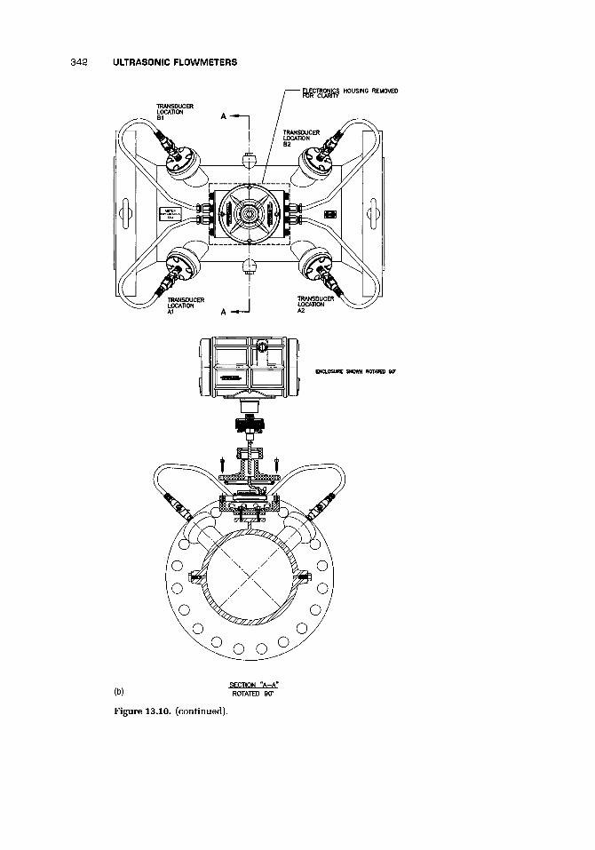
342 ULTRASONIC FLOWMETERS
HOUSING REMOVED
TRANSDUCERLOCATION .B1 A
ENCLOSURE SHOWN ROTATED 9 7
(b)SECTION "A-A"ROTATED 90*
Figure 13.10. (continued).

13.8 GENERAL PUBLISHED EXPERIENCE IN TRANSIT-TIME METERS 343
(c)
Figure 13.10. (continued).
SECTION "A-A"ROTATED 90 '

344 ULTRASONIC FLOWMETERS
13.9 APPLICATIONS, ADVANTAGES, AND DISADVANTAGES
Manufacturers suggest that the meters are suitable for any homogeneous liquid thatadmits an ultrasonic wave (e.g., service water, seawater, and drainage), but not ifbubbles or turbidity are present. However, one manufacturer cites applications suchas city water, sewage water, industrial water, river water, sea water, and oil.
With its introduction into some national regulations for fiscal measurement ofoil and gas, this meter is becoming more widely used in gas export stations (Sloet andde Nobel 1997) and flow line measurement (Agricola 1997). They can also provideself-monitoring (Sakariassen 1997).
Particular applications include:
• Flare-gas flow measurement (Raustein and Fosse 1991 of the NorwegianPetroleum Directorate) where ±5-10% measurement uncertainty appears to becommon-This maybe (Mylvaganam 1989) in a pipe of, say, 36-in. (0.91-m) diam-eter with velocities ranging from 0.3 to 80 m/s. The low flare is activated for 95%of the time, but this constitutes only about 10% of the gas flared. The pressureis only about 0.7 bar.
• Water flow in steam power plants, and hydroelectric plants (Erickson and Graber1983).
• Pipeline management by clamp-on transit-time meters (Baumoel 1996) com-bined with leak detection.
• Nuclear fuel processing plant (Finlayson 1992) for both nonradioactive and ra-dioactive liquid flows.
• Fiscal gas metering (Hannisdal 1991).• A general-purpose gas meter capable of use with air flows, nitrogen, argon, and
chlorine.
Advantages include (Beeson 1995, Mylvaganam 1989) its nonintrusiveness, lackof moving parts, compactness, high rangeability, ease of installation, cost savings andimprovements in maintenance with self diagnostics, accuracy unaffected by build-upof contaminants, fully pigable, bidirectional flow capability, no line pipe restriction,and unaffected by pulsation flow. NorAm found that a single-path flowmeter couldbe installed in a day, and hot-tapping can be used under pressure. Self-checking usingsignal strength and quality alert the instrument technician to problems.
de Vries et al. (1989) claimed that transducers could be installed in undergroundgas pipes from ground level, so that, using reflection mode, a measurement uncer-tainty of 2% could be achieved with a repeatability of 0.2%.
Problems when applied to gases include low efficiency of launching waves dueto impedance differences, absorption increases with frequency, and beam bendingin large flow lines with high speed flow.
Adverse effects may be present with pulsating flow, and Beeson (1995) suggestedusing asynchronous sampling techniques.
Many would share Cairney's (1991) sentiment that "it is a pity that [the transit-time clamp-on flowmeter] is still associated with Doppler meters "

13.10 DOPPLER FLOWMETER 345
13.10 DOPPLER FLOWMETER
13.10 .1 SIMPLE EXPLANATION OF OPERATION
The doppler flowmeter depends on the doppler frequency shift, which occurs whensound bounces off a moving object as shown in Figure 13.11. In the doppler meter,the waves need to reflect off something moving with the flow. If they reflect offa stationary object, then they retain their wavelength and frequency. If, however,they reflect off a moving object, the wave fronts will hit the moving object with atime interval that is not the same as their period in a stationary medium. As a result,the reflected wave will have a new period, frequency, and wavelength. It is almostinvariably a clamp-on design for liquids. Figure 13.11 is a diagram of the effect.
The arrangement for typical commercial doppler meters is also shown inFigure 13.11. The transmitting and receiving transducers may be in the same blockand held on the outside of the tube. On the other hand, they may be in separateblocks (Figure 13.11) and can then be positioned on the same side or on oppositesides of the tube.
We are now faced with one of the major uncertainties in the operation of thesedevices. What is the velocity of the reflecting object compared with the axial meanvelocity of the flow in the pipe? This depends (Figure 13.11) on
• what the reflecting surface is,• where the reflecting surface is, and• the velocity of the object and its relative velocity to the flow in size and angle.
Transducers
Cy'/Z^ /
SV c Particle which ,? > V reflects/ y X ^ ^ acoustic
/ ^ ^ beam
V
Alternative positionfor receiving transducer
Figure 13.11. Diagram of doppler flowmeter showing the doppler effect andtypical arrangements of the transducers for a commercial device.

346 ULTRASONIC FLOWMETERS
We can start by taking the simplest assumption that the particle is moving withthe flow and that path, therefore, makes an angle with the axis of 6. So in terms ofV, the velocity in the pipe is
Af = 2ft-cos6 (13.11)
We can obtain a typical value of Af assuming a transmission frequency ft of,say, 5 MHz and a flow rate of water of 10 m/s. A f will then have the value, assuming1414 m/s for sound, of about 50 kHz. Clearly, this will not be one sole frequencycoming back from the fluid, but rather a range of frequencies, and some method willbe built into the converter to identify the favored frequency.
At least one manufacturer appears to offer a profile measurement capability. Thisis usually achieved by range gating the returning signal so that the distance of pen-etration into the pipe is known and hence the velocity at that point.
Uncertainty claims may be ±2% of full scale, although great care and understand-ing of the flow is needed in gaining confidence in the reading from these devices.
Poor mounting can cause spurious reflections, and pipe vibration may give falseflow signals. Transmit and receive may be in one transducer block or may be inseparate blocks allowing positioning on opposite sides of the pipe (Figure 13.11).
13.10.2 OPERATIONAL INFORMATIONOne manufacturer suggests that installation should allow 6D upstream and 4Ddownstream. Transducers should be mounted adjacent to each other for large pipesbut on opposite sides for small pipes. I noted the following comment: "... the pulsesare reflected from a large area of the flow profile, giving a good representation ofmean velocity. Repeatability of measurement is to specification, and with 'on-site'calibration checked, volumetric accuracy is assured/' I would be less certain than thisparticular manufacturer, until I had the experience of a prolonged set of calibrationsand a usage log that showed consistency.
Ranges are from, say, 0.3 to 6 m/s, with a temperature range of -20 to 80°C.
13.10.3 APPLICATIONS, ADVANTAGES, AND DISADVANTAGESCairney (1991) commented on doppler flowmeters saying that "these were the firsttype of ultrasonic flowmeter produced commercially. Experience has shown thatthey were oversold as an all-purpose flowmeter. When there were particles in thefluid measured they have been of some use, but most fluids flowing through powerstation pipelines are clean, which makes them far less effective."
Manufacturers suggest that these meters can be used for mining slurries, coalslurries, sewage, sludge, raw water, sea water, pulp (paper), acids, emulsion paint,fruit juice, yogurt, citric acid, glucose, contaminated oil, cement slurry, lime slurry,and industrial effluent.
13.11 CORRELATION FLOWMETER
13.11 .1 OPERATION OF THE CORRELATION FLOWMETERIf two beams cross the flow at a known distance apart L, as in Figure 13.12(a), andthe received signals are compared, as in Figure 13.12(b), to find a similar pattern, the

1 3 . 1 1 CORRELATION FLOWMETER 347
pattern for channel B will be found to bedisplaced a time rm from that for channelA. From this, it is simple to deduce that theflow has taken time rm to move a distanceL or
V=— (13.12)
Correlating the two signals requires somecomplex electronics. The fluctuation in thesignal must be adequate, and for this rea-son, it will probably need to be created ar-tificially by an upstream disturbance in theflow, if heavy turbulence, bubbles, secondphase, etc., are absent naturally. The math-ematical concept of cross correlation is de-fined by the equation (Keech 1982)
1 rTRyx(r) = limr-oo ~ / y(t)x(t + x)dt
Transmitters
(13.13)where x{t) and y(t) are the upstream anddownstream signals, respectively. The valueof time delay rm corresponding to the max-imum of Ryx(r) provides a measure of the
Flow
(a)
ReceiverA
A Receivers B
L.
ReceiverB
•-»*"* > Time
A A iv. • • Time
(b)
Figure 13.12. Correlation flowmeter: (a) Diagram ofthe geometry; (b) Traces from channels A and B.
flow transit time between the two beamsspaced I apart. The calculation of the integral in Equation (13.13) is achievablewith modern computation. The problem is to do it cheaply and fast. For instance,sufficient precision may be achievable by using only the polarity of the signal, and bycutting the signal into sufficiently small bits of fixed size, but by varying polarity, theintegration may be simplified and speeded up without significant loss of precision.(However, see Yang and Beck 1997.)
It has found a particular niche in multiphase flows where the disturbance to thesignal will be substantial. However, Keech (1982) suggested that some form of valida-tion is needed because the system can give incorrect estimates of velocity: spuriousnoise can give a correlation, decay of disturbances at low flows, other movementsuch as cavitation-generated shock waves or intense pressure waves, and oscillatoryflows. Multichannel devices may overcome some of these effects.
13 .11 .2 INSTALLATION EFFECTSPaik et al. (1994) used clamp-on transducers with 1-MHz crystals, 35° wedges,and 2D or 3D spacing in some tests of installation effects. Their baseline testswere with 120D upstream straight pipe. The errors found by them are shown inTable 13.9.
There may be other experimental studies of installation effects of which I am notaware, but because this is the only data provided in this book, it should probably beused with caution.

348 ULTRASONIC FLOWMETERS
Table 13.9. Error in signal due to upstream fittingsDiameters Upstream
Fitting 5 10 20 30
Single elbow -7% -4% (-2%) (-2%)Double elbow
out-of-plane -2 to -4% +5% +2 to 6% 0 to 4%Double elbow
in-plane -6% - 5 % -2% -2%() possible scatter.
13 .11 .3 OTHER PUBLISHED WORKKing (1988; cf. King et al. 1988 and Sidney et al. 1988a, b) mentioned the develop-ment of an ultrasonic cross-correlation meter for multiphase flow at the NationalEngineering Laboratory, Scotland, in collaboration with Moore, Barrett, and Red-wood. This development undoubtedly exploits one of the most important applica-tions of this technique, and increasingly sophisticated electronics should allow moreinformation about the flow components and their velocities to be deduced.
Coulthard and Yan (1993c) provided one of the many reviews of correlationflowmeters. They review results for two-phase mixtures:
Solids and liquids Satisfactory operationOil and gas At void fractions up to 25% and velocities
up to 7 m/s scatter of results was ±4.5%without mixing and ±2% with mixing
Single-phase gas and liquid are also usable but may need a bluff body to enhancethe signal.
Xu et al. (1994) described a clamp-on ultrasonic cross-correlation flowmeter forliquid-solid two-phase flows, with brief indications of how the various componentsoperate. Calibrations of these meters against an electromagnetic meter gave differ-ences of about ±5% for a 0.4% by weight paper pulp flow and about ±3% for a crudeoil flow.
Recent work by Battye (1993) suggested measurement uncertainty over 10:1of ±2% with 0.5% scatter, but that temperature variation in the acoustic path, ifnot allowed for, might reduce linearity. Other work by Kim et al. (1993a) suggested±2.2% or for clamp-on ±2.8%. A very recent paper by Yang and Beck (1997) claimedthat, with a highly intelligent cross-correlator, a measurement accuracy of 1% couldbe achieved.
Lemon (1995) discussed a technique referred to as acoustic scintillation flow mea-surement; it appears to refer to, or be related to, cross-correlation flow measurementusing the disturbances caused to the ultrasonic beams in traversing the flow.
It should be remembered that even though cross-correlation has been used withultrasonics and included here for that reason, it has much wider application. Chenet al. (1993) reported work using two pairs of radiation sensors. Their applicationwas to medium-consistency pulp in the paper industry. Flows approach Newtonian
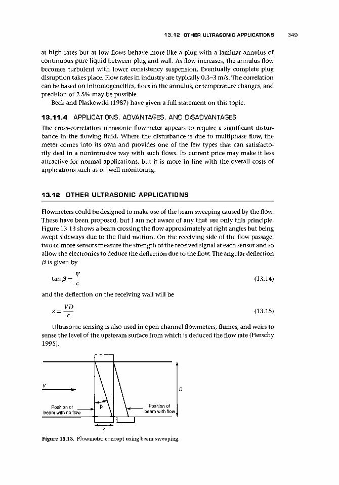
13.12 OTHER ULTRASONIC APPLICATIONS 349
at high rates but at low flows behave more like a plug with a laminar annulus ofcontinuous pure liquid between plug and wall. As flow increases, the annulus flowbecomes turbulent with lower consistency suspension. Eventually complete plugdisruption takes place. Flow rates in industry are typically 0.3-3 m/s. The correlationcan be based on inhomogeneities, floes in the annulus, or temperature changes, andprecision of 2.5% may be possible.
Beck and Plaskowski (1987) have given a full statement on this topic.
13 .11 .4 APPLICATIONS, ADVANTAGES, AND DISADVANTAGES
The cross-correlation ultrasonic flowmeter appears to require a significant distur-bance in the flowing fluid. Where the disturbance is due to multiphase flow, themeter comes into its own and provides one of the few types that can satisfacto-rily deal in a nonintrusive way with such flows. Its current price may make it lessattractive for normal applications, but it is more in line with the overall costs ofapplications such as oil well monitoring.
13.12 OTHER ULTRASONIC APPLICATIONS
Flowmeters could be designed to make use of the beam sweeping caused by the flow.These have been proposed, but I am not aware of any that use only this principle.Figure 13.13 shows a beam crossing the flow approximately at right angles but beingswept sideways due to the fluid motion. On the receiving side of the flow passage,two or more sensors measure the strength of the received signal at each sensor and soallow the electronics to deduce the deflection due to the flow. The angular deflection(3 is given by
tan/3 = -
and the deflection on the receiving wall will be
VDz=
(13.14)
(13.15)
Ultrasonic sensing is also used in open channel flowmeters, flumes, and weirs tosense the level of the upstream surface from which is deduced the flow rate (Herschy1995).
Position ofbeam with no flow
Position ofbeam with flow
Figure 13.13. Flowmeter concept using beam sweeping.

350 ULTRASONIC FLOWMETERS
In vortex meters, one method of sensing the oscillation of the shedding is ultra-sound, which is disturbed by the vortices and provides a signal that can be used toextract the frequency of shedding.
Coulthard and co-workers have also suggested using the vortex-shedding com-bined with a correlation-sensing system to obtain flow measurement. It should benoted in this technique that vortices may move faster than the fluid.
Teufel et al. (1992) described a new technique for measuring the profile in pipesand applied it to oscillating flows. The object of the paper was to compare LDV andthe new ultrasonic velocity profile sensor. They saw the techniques as complemen-tary, and it is possible that the second may offer an industrial approach where profiledetermination is important.
Olsen (1991) described tests of what appeared to be an anemometer using sonicand ultrasonic signals and allowing velocities in a wind tunnel to be measured inthree directions simultaneously.
Joshi (1991) describes a surface-acoustic-wave (SAW) flow sensor. The oscillationfrequency is temperature dependent, and so if the element is heated above ambientand placed in the flowing gas, the frequency will be flow-rate dependent.
Guilbert et al. (1996) used a pulse of heat through the pipe wall to mark theliquid, and the passing of the marked liquid was sensed by an ultrasonic beam usingthe transit time across the pipe for cold and hot liquid.
13.13 CHAPTER CONCLUSIONS
One feature of ultrasonic flowmeters is the large amount of information avail-able from the system, but not completely used, which will give indication of op-erating changes or problems. In my earlier book (1988/9), I suggested that ultra-sonic technology might develop a clamp-on meter (possibly a master meter) thatsensed:
• wall thickness,• the quality of the inside of the tube,• the turbulence level,• profile from a range-gated doppler system,• flow measurement from a transit-time system,• correlation to provide information about a second phase,• density from the impedance and sound speed, and• condition (self) monitoring.
Such a device could measure diameter and other pipe details and could programa much simpler device for permanent installation at the site.
Some of these features now appear together. Sanderson and Torley (1985) com-bined wall thickness and some dimensional and condition monitoring, with intelli-gent control. Range-gated doppler has been exploited in medical applications. Birchand Lemon (1995) discussed the use of doppler on multiple paths with range gatingto obtain profiles of flows in open channels and discharges. A commercial devicemay allow operation in both transit-time and doppler modes. Correlation has been

13.A.1 SIMPLE PATH THEORY 351
used for multiphase oil and gas flow measurement. Guilbert et al. (1996) have usedthe device for mass flow measurement. Lynnworth (1990) has found that the phasevelocity of flexural waves in the wall of small diameter pipes was dependent on thedensity of the liquid inside. As the technology becomes more widely accepted, themicroprocessor control is likely to become more powerful and to introduce multiplefacilities.
The extraordinary success in developing instruments for domestic gas measure-ment, which are within the tight budget for the utilities, operate off a battery with10 years or more of life, and have sophisticated external communication ability, will,with little doubt, provide precursors of much more in this area.
Perhaps the ultrasonic flowmeter is the realistic rival to the Coriolis meter in gasmass flow measurement, at lower cost, and of greater versatility.
Much development work continues as shown by the preceding references. Braggand Lynnworth (1994, cf. Lynnworth 1989, 1994) proposed the use of a single portwith two axially spaced transducers. As an example, they suggested that a spacingof 60 mm axially for a velocity of 1 m/s and a sound speed of 343 m/s would resultin a l-/xs transit-time difference or a 10-ns resolution (i.e., 1%). To avoid cross-talkbetween the transducers, they investigated O-rings of various materials and foundthat silicone was highly attenuating.
The application at which this is aimed is firstly noncombustible gases, in whichcategory some stack gases fall.
They also suggested that two angled transducers in the same port can transmitand receive a signal that forms a triangular path in the pipe cross-section and thussenses swirl. Lynnworth et al. (1994) also developed a profile-measuring methodusing the one port with either a traversing reflector or a series of fixed reflectors.
Ultrasonics combined with other methods (e.g., Guilbert et al. 1996) such asthermal marking may provide new scope.
Another interesting development is the insertion meter of Rawes and Sanderson(1997) discussed in Chapter 18, which could revolutionize in situ calibration inliquids and gases.
This is such a powerful technology that it is starting to be seen as capable ofmeeting fiscal demands for metering liquid hydrocarbons; therefore, limits of itsprecision and reasons for baseline instability need to be understood urgently.
APPENDIX 13. A
Simple Mathematical Methods and Weight FunctionAnalysis Applied to Ultrasonic Flowmeters
13.A.1 SIMPLE PATH THEORY
Transit-TimeFigure 13.2 provides a diagram on which to base the mathematics. We can work interms of trigonometric functions or dimensions.

352 ULTRASONIC FLOWMETERS
We start with the downstream-going wave and note that its speed will be greaterthan the sound speed by the component of the flow in the direction of the path.This component is VcosO. The distance to be traveled is D cosec 0, where D is thepipe diameter so that the time taken for the downstream wave to travel from thetransmitter to the receiver is
t* = ^ (13.A.1)
A similar expression for the upstream wave time tu is
Dcosec0 , „ A rtXtu = (13.A.2)c-Vcos<9 v '
We can now obtain the difference between these two wave transit times (Figure 13.3)
At=tu-td
Dcosec0 Dcosec0c-VcosO c+VcosODcosecO/c DcosecO/c
= V V1 cos 0 1 H— cos 0
c cCombining the two fractions on the right-hand side over a common denominatorand ignoring terms in (V/c)2, we obtain
IVDcotO / I * A ^At = (13.A.3)
Thus we see that, provided we know the speed of sound, we can find the value of Vfrom the time difference and the geometry of the meter. The requirement to knowthe value of c is not difficult if we measure, as well as the time difference, the actualtransit times each way and take the mean tm. We can make the approximation
£ = (tu - At/2)(td + At/2)= tu*d + At(tu - *d)/2 - (At)2/4= tu*d + At(At)/2 - (At)2/4= tuta + (At)2/4« tuta (13.A.4)
where, using values in Table 13.1, we have neglected a term of about 10~6. We cannow replace c2 by L2/tutd and cot# by X/D. We can then rewrite Equation (13.A.3)by
2 ^ (13.A.5)
From this, we can obtain Equation (13.5).

13.A.2 USE OF MULTIPLE PATHS TO INTEGRATE FLOW PROFILE 353
Sing-AroundAn alternative way to eliminate sound speed is the sing-around method (Figure13.4) discussed by Suzuki et al. (1975, cf. 1972). In this method, each of the paths,upstream and downstream, is operated in such a way that when the pulse is receivedby the receiving transducer, it triggers a new pulse from the transmitting transducer.Thus the frequency of pulses is dependent on the velocity of sound and of the flow.We can obtain the period between pulses from Equations (13.A.1) and (13.A.2), andthe pulse frequency will be the inverse of the period, or for the downstream-goingpulses
f c+ VcosOf _ (13.A.6)/d Dcosec<9 v ;
A similar expression for the upstream pulse train is
. c- VcosO/u = (13.A.7)' Dcosec6>
If we now take the difference between these frequencies, we obtain
2 f cos6>sin6>
= Vsin20/D (13.A.8)
We can write this in terms of dimensions, since 2cos# sinO = 2DX/L2, as
Af = 2VX/L2 (13.A.9)
which has the virtue of relating V to the frequency difference without requiring thevalue of c, the sound speed. Again we can obtain typical values for the frequenciesfrom Table 13.2 (Baker 1988/9). Making the approximation that V is constant acrossthe pipe, we can obtain Equation (13.7).
13.A.2 USE OF MULTIPLE PATHS TO INTEGRATE FLOW PROFILE
The preceding simple analysis assumed that the flow profile is uniform. In fact, if weallow for varying velocity along the path of the ultrasonic beam, Equation (13.A.3)may be rewritten in the form of an integral
V(y)dylong
2 (c2
The flowmeter obtains the average velocity, Vm, along the path of the beam.

354 ULTRASONIC FLOWMETERS
For integration along the chord shownin Figure 13.A.I,
2cot0At =
(13.A.11)If the path is on the diameter, two
extremes of laminar profile and uniformprofile yield a At ratio for equal volumetricflows of 4:3. Thus an ultrasonic flowmeterwith diametral sensing has an intrinsic cal-ibration shift across the laminar-turbulentprofile change approaching 33%.
Baker and Thompson (1975, 1978) showed the improvement possible by usingapproximately midradius transducers and recalculating Equation (13.A. 11) for valuesof h % a/2. By using the approximate expression for the turbulence velocity profileof
Figure 13.A.I. Geometry of the pipe cross-section forchordal integration.
•H)1/w
(13.A.12)
where n varies with Reynolds number as
Re 4 x 10³ 2.3 x 10⁴ 1.1 x 10⁵ 1.1 x 10⁶ 2.0 x 10⁶ to 3.2 x 10⁶
17 6.0 6.6 7.0 8.8 10
the signal variation can be obtained as in Figure 13.6.The basis for using more than two paths lies in the mathematics of numerical
integration. Linked to the name of Gauss, it can be shown that a polynomial of theform
f{f) = Co + d t + c2t2 + cst3 + • • • + c2n+1 t2n+1
can be precisely integrated as
£ f(t)dt = Ao f(fy) + Ax f ft) + A2 f(t2) + • • • + An (13.A.13)
Or a polynomial of degree In + 1 or less can be correctly integrated by an ex-pansion such as in Equation (13.A. 13) provided the constants An and the positionstn are correctly chosen. It is also possible to show that an integral can be rearrangedto the interval - 1 to +1. Thus with four positions and with suitable weighting, theintegral of a polynomial of up to order seven can be correctly evaluated.
It is as a result of considerations such as these, and possible refinements basedon likely profiles in the flow, that weightings for multiple paths (cf. Vaterlaus 1995)have been obtained.

13.A.4 DOPPLER THEORY 355
13.A.3 WEIGHT VECTOR ANALYSIS
Hemp (1982) has developed the ideas from electromagnetic flowmeter theory forultrasonic flowmeters. As in the case of electromagnetic flowmeters, the conditionfor an ideal flowmeter, one where the signal is independent of flow profile, is
V x W = O (13.A.14)
and Hemp obtained a flow signal expression using his reciprocal theory of
±(U$Z) - U^I = 2 f Vs • WdV (13.A.15)
where the negative sign is for electromagnetic and/or magnetostrictive transduc-ers and the positive one for electrostatic and/or piezoelectric, I is the driving cur-rent, L/j(2) and U^ are the received voltages, and Vs is the undisturbed flow. Theweight vector is then given in terms of pm the mean density in the meter and v0 theacoustic field for two distinct cases (1) and (2) when opposite transducers transmitas
W = p
Hemp suggested that a flowmeter in a rigid-walled duct with plane wave modes,a meter with radial transmission, and a meter with a large area transmission (e.g.,the industrial design for small pipes) are approaching ideal configurations.
In addition to the fundamental weight vector [Equation (13.A. 16)], it is possibleto define weight vectors for phase shift and amplitude shift (in sine wave operation)and for pulse operation (Hemp 1998).
13.A.4 DOPPLER THEORY
Figure 13.11 is a diagram of the effect. A wave approaches a particle moving withvelocity component v in the direction of the acoustic wave, which has a velocityc, and is reflected. The velocity remains at c relative to the medium after reflectionbecause sound speed is not affected by frequency (within reasonable limits). But theperiod between two waves being reflected will not be kt/c. The wave will hit theparticle at a velocity c-v, and so peaks will hit the particle every kt/(c - v) seconds.But successive peaks will make contact with the moving particle at different particlepositions, so the second peak will hit the particle kt/(c - v) seconds after the firstbut will then need to travel ktV/(c — v) to reach the starting point of the first peak.This additional travel takes ktV/c(c - v) seconds. So the time between peaks is rgiven by
ktl + v/c (13.A.17)c 1-v/c K }

356 ULTRASONIC FLOWMETERS
Expanding Equation (13.A.17) using the binomial theorem, the frequency of thereflected wave fT becomes (ignoring ^ )
Hence, the frequency shift A f is given by
= 2ftV- (13.A.19)

CHAPTER 14
Mass Flow Measurement UsingMultiple Sensors for Single- andMultiphase Flows
14.1 INTRODUCTION
The measurement of mass flow, a fundamental requirement for any fluid, has beenan elusive goal due to the problems of developing a suitable flowmeter. Despite this,the availability of mass flowmeters has increased greatly over the last 15 years. Thisis partly due to the increasing value of products (Hall 1990), but it is also due toan increasing realization that volumetric flow measurement is often inappropriate.In addition, the advent of the Coriolis flowmeter has stimulated engineers to findother mass flowmeters. General reviews of mass flowmeters were given by Sprostonet al. (1987), Betts (1990), and Medlock and Furness (1990).
Mass flow measurement is commonly categorized as direct (true) or indirect (in-ferential). However, it may be useful to allow a few more than two categories.
a. True (direct) mass flow measurement by a single instrument is rare. It appearsthat to achieve it we need to use one of the fundamental acceleration laws. Wecan do this by creating:• the force (or torque) resulting in a linear (or angular) acceleration (Chapter 16
describes an example) or• the force that produces Coriolis acceleration (Chapter 17).
b. Fluid-dependent thermal mass flow measurement uses the temperature rise re-sulting from heat addition but is affected by other parameters such as the specificheat of the fluid (Chapter 15).
c. Multiple differential pressure flowmeters used in a dedicated system (Section14.2) depend on the nonlinearity of the flowmeter equation.
d. Indirect (inferential) mass flow measurement combines volumetric flow rate ormomentum flow rate with a density measurement (Section 14.3). (An alternativeis to combine volumetric and momentum flow measurements.)
e. Multiphase flow measurement almost always requires multiple measurements(Section 14.4).
14.2 MULTIPLE DIFFERENTIAL PRESSURE METERS
Before turning to the one method that is commercially available, for completenesswe shall look at two methods that have been suggested but, to my knowledge, havenot been used commercially.
357

358 MASS FLOW MEASUREMENT USING MULTIPLE SENSORS
Pump
Figure 14.1. Twin venturi system.
Twin Venturi SystemThe twin venturi system depends on the use of two identical venturi meters (orother differential pressure devices) that are arranged in parallel balanced paths asshown in Figure 14.1. By means of a metering pump, which transfers qvp from oneline to the other, the flows may be unbalanced. If the pump is off, so that the flowis split equally between the two paths and is, therefore, the same in each meter,the differential pressure across each meter is also the same. If the pump is started,then one venturi meter has a lesser and the other a greater flow passing through it.The pressure difference between the throat pressures A/?AB is then measured, and themass flow rate qm is deduced.
We first note that the pressure drop to the throat of each venturi is given by
ApA = ApB = K(qm/2)2/p (14.1)
where K is a constant, p is the density of the fluid, and qm is the total mass flowthrough both Venturis, and so qm/2 is the total mass flow through one of the Venturiswhen the flows are equal.
If the main flow qm splits equally, then if the pump is started and transfers fluidas shown, and provided that the upstream pressures at inlet to the Venturis are notaffected by the transfer, the equation for the pressure drop to the throat of A will be
(14.2)
(14.3)
and to the throat of B
ApB = K(qm/2-pqvp)2/p
Thus the differential pressure will be
= K(qm/2 + pqvV)2/p - K(qm/2 - pqvp)2/p
= K (q^/4 + pqmqvP + P2<£p)/p - K [q^/A - pqmqvp + p2q2p)/p
= 2Kqmqvp (14.4)
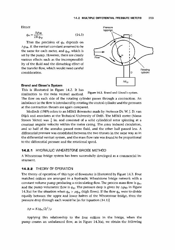
14.2 MULTIPLE DIFFERENTIAL PRESSURE METERS 359
Hence Pressuretappings
qm=^PL (14.5)
Thus the precision of qm depends onB, K the venturi constant assumed to be
the same for each meter, and qvp, which isset by the pump. However, there are clearlyvarious effects such as the incompressibil-ity of the fluid and the disturbing effect ofthe transfer flow, which would need carefulconsideration.
Brand and Ginsel's SystemThis is illustrated in Figure 14.2. It hassimilarities to the twin venturi method.
Rotatingcylinder
Figure 14.2. Brand and Ginsel's system.
The flow on each side of the rotating cylinder passes through a contraction. Animbalance in the flow is introduced by rotating the central cylinder and the pressuresat the contraction throats are again compared.
Medlock (1989) refers to an MSM1 flowmeter made by Professor Dr. W. J. D. vanDijck and associates at the Technical University of Delft. The MSM1 meter (MassaStroon Meter) was | in. and consisted of a solid cylindrical rotor spinning at aconstant angular velocity within the meter casing. The rotor induced circulation,and so half of the annulus passed more fluid, and the other half passed less. Adifferential pressure was established between the two throats in the same way as inthe differential venturi system, and the mass flow rate was found to be proportionalto the differential pressure and the rotational speed.
14 .2 .1 HYDRAULIC WHEATSTONE BRIDGE METHOD
A Wheatstone bridge system has been successfully developed as a commercial in-strument.
14.2 .2 THEORY OF OPERATION
The theory of operation of this type of flowmeter is illustrated by Figure 14.3. Fourmatched orifices are arranged in a hydraulic Wheatstone bridge network with aconstant volume pump producing a recirculating flow. The process mass flow is qm,and the pump volumetric flow is qYp. The pressure drop is given by A/?BD in Figure14.3(a) for the situation when qm > pqvp (high flows). If the flow qm were to divideequally between the upper and lower halves of the Wheatstone bridge, then thepressure drop through each would be [as for Equation (14.1)]
Ap = K(qm/2)2/p
Applying this relationship to the four orifices in the bridge, when thepump creates an unbalanced flow, as in Figure 14.3(a), we obtain the following

360 MASS FLOW MEASUREMENT USING MULTIPLE SENSORS
(a) (b)
Figure 14.3. Wheatstone bridge flowmeter: (a) High flows; (b) Low flows.
expressions:
= K(qm/2 + pq,P/2)2/p - K(qm/2 - pqyp/2)2/p
Kq,'vp
(14.6)
(14.7)
(14.8)
(14.9)
Similarly, for the case of Figure 14.3(b), the pressure difference is given by ApAC
when qm < pqvp (low flows), and we obtain
ApAc = ApAB + ApBC
- -K(qm/2 - pqyv/2)2/p + K(qm/2 + pqvp/2)2/p (14.10)
(14.11)
(14.12)^vp
14.2 .3 INDUSTRIAL EXPERIENCE
The meter consists of four precisely matched orifices forming the hydraulic Wheat-stone bridge. A recirculating pump establishes reference flow in the bridge. At zeromeasured flow rate, pressure drop across the bridge is zero. As measured flow passesthrough the meter, it upsets the balance in the bridge such that a differential pressuresignal, which is linear and proportional to true mass flow rate, is generated.
The resulting flowmeter is claimed to give true mass flow rate and may be unaf-fected by changes in fluid, temperature, density, and viscosity. It can be of stainlesssteel construction and capable of operation at elevated temperatures and with lowlubricating liquids.

14.3 MULTIPLE SENSOR METHODS 361
Typical flow ranges may be
• 0-2.3 kg/h (0-5 lb/h) for microflows with a turndown of 50:1 and a minimumflow of 0.05 kg/h;
• 0-900 kg/h (0-2,000 lb/h) for low flow ranges and 0.5 kg/h minimum flow forlow ranges; and
• 0-23,000 kg/h (0-50,000 lb/h) for high flow ranges with about 100:1 turndown.
A wide range version in the low flow range may be capable of 500:1 turndown.Best accuracy may be of order 0.5% of rate plus 0.02% FSD, and repeatability 0.25%of rate although in some designs an additional amount based on FSD may be added.Pressure drop may be in the range from about 0.1 to 2 bar. Depending on the design,fluid temperature may be in the range from about -18 to +150°C and pressure upto about 67 bar gauge.
14.2.4 APPLICATIONSThis device is particularly suited for fuel flow measurement applications such asengine emission control and fuel economy testing. Other applications may be fuelefficiency testing in boilers. It produces an output signal that is linearly proportionalto mass flow rate.
14.3 MULTIPLE SENSOR METHODS
If the fluid has unknown properties, we shall probably need to combine the flowmeasurement with a density measurement. However, if the fluid has known param-eters, we may be able to use equations that describe the fluid's state. The followingare examples of both.
• A volumetric meter (e.g., turbine) with density, or pressure and temperature mea-surement. This is a relatively common practice. A combination of electromag-netic flowmeter with a gamma density-sensing cell has been available commer-cially. The mass flow will be given by
qm = pVA (14.13)
where p is the fluid density, V is the mean velocity through the meter, and A isthe cross-section of the meter. There is likely to be a correct position at which tomeasure the density. There will, therefore, be an overall uncertainty stemmingfrom the various components
qm p V A
or the equivalent root-mean-square expression. Similar error calculations will beappropriate to the other methods mentioned here.
• A vortex meter that combines frequency measurement with measurement of lifton the shedding body. Itoh and Ohki (1993) claim a vortex flowmeter design thatobtains mass flow rate by the use of the lift on the central body divided by the

362 MASS FLOW MEASUREMENT USING MULTIPLE SENSORS
frequency of pulsation. This depends on the assumption that the lift coefficientand the Strouhal number are both constant, so that the lift is proportional top V2, and the frequency is proportional to V. As a result, the ratio is proportionalto pV.
• Ultrasonic flowmeters. The speed of sound is related to the density
c2 = yp/p (14.15)
where y is the ratio of the specific heats, and p is the density of the fluid. Asimilar equation for liquids is
c2 = l/(ksP) (14.16)
where ks is the adiabatic compressibility. Because c2 appears in the equation fortime-of-flight ultrasonic meters, it can be combined through these equations togive velocity times density and hence mass flow. This assumes that for gases yis constant, which is a good approximation for air. The value of y is dependenton the number of atoms in the gas molecule. The value of p will be needed. Fora liquid, the value of ks will be needed (Baker 1976).
• Alternatively for ultrasonic flowmeters the impedance of the fluid is related tothe density and may be used to obtain its value (Guilbert and Sanderson 1996a).
• A differential pressure flowmeter with the density of the fluid obtained ei-ther directly or, say, for a gas via pressure and temperature measurements (cf.Figure 5.20).
• A combination of velocity measurement to obtain V, with momentum pV2,allows the value of p V to be found.
Medlock used the term hybrid (1989) to describe meters combining momen-tum sensing and volume sensing, such as the venturi tube with an electromagneticflowmeter built into it or venturi and turbine meters (Frank et al. 1977, Reimann etal. 1982) or the turbine meter that also senses drag on the wheel or on a separatedrag plate (Reimann et al. 1982) or gauze (Cole 1985). Wong et al. (1981) suggestedthe use of the pressure drop in a swirl generator in combination with a venturi.
14.4 MULTIPLE SENSOR METERS FOR MULTIPHASE FLOWS
14.4.1 BACKGROUNDThere is a growing need to measure the flow of fluids, which consist of more thanone component. The nature of the second component may or may not be known,and the proportions or indeed the existence of the second or even third componentmay not be known. The reasons for this growing need are the increasing value ofsuch fluids, being used in an ever widening variety of processes, and the increasingrequirement to conserve energy. The fluids involved range across wide industry areasas diverse as food processing and subsea hydrocarbon extraction, but at present thetechnology appears mainly to be driven by the latter.
Against this background, most flowmeters have been designed to measure thesingle-phase flow of a Newtonian fluid but, despite this, are being called on,
14.4 MULTIPLE SENSOR METERS FOR MULTIPHASE FLOWS 363
sometimes unknowingly, to handle more complex fluids. Baker (1991a) attemptedto draw together the references and the most useful data on the likely response ofbulk flowmeters when placed in such flows (cf. Baker 1988, 1989). More recently,Whitaker (1993) has reviewed the latest developments.
These complex flows (discussed briefly in Chapter 2) have been extensively stud-ied, and flow pattern maps have been developed to indicate the conditions underwhich the various flow regimes occur (Butterworth and Hewitt 1977, Hetsroni 1981).However these may be limited in their application to particular fluid combinationsand pipe sizes. To measure the flow in any of these regimes requires a large number ofvariables to be interpreted from measurements. Mixing or conditioning of the flowmay be possible in some applications but may not greatly improve the situation.Separation of the components is also possible in some applications, and some of thedesigns mentioned in Section 14.4.3 attempt this, but again this is not possible orconvenient in many applications.
Some of the earliest data appear to be those that relate to a nuclear plant underemergency conditions. Experiments were undertaken, and special designs and com-binations of meter were tried to obtain a system that would signal fault conditions inthe nuclear reactor duct flows. The expected changes in the flows were considerable,and so precise flow measurements were not always essential.
Dykesteen (1992) identified the development of small oil wells in the North Sea,where a platform would be too costly, as one reason for needing a multiphase meter.Subsea reservoir management will need to take place without the use of a separator,and where different satellite wells are operated under different licences, individualflow measurement will be required. The multiphase meter should, if possible, providecomponent fractions, component velocities, and component densities.
14.4 .2 CATEGORIZATION OF MULTIPHASE FLOWMETERS
Dykesteen (1992) suggested that multiphase meters operated in one of three ways:
i. by total separation of components;ii. by measurement of the multiphase flow rate but separation of a sample for com-
ponent measurement; oriii. by in-line measurement of all parameters.
For applications other than oil production, (iii) has usually been the aim. An exampleis the early work in the nuclear industry such as the combination of turbine andtarget meters for loss-of-coolant nuclear applications (cf. Goodrich 1979 and otherpapers at the same conference). A more recent example is the venturi meter, whichhas been combined with both capacitance and gamma densitometer (Kratzer andKefer 1988, Smorgrav 1990) with some impressive results [Figures 14.4(a,b)]. Oneadvantage of the venturi is that it appears to homogenize the flow. Other examplesare Arnold and Pitts' (1981) proposal for a positive displacement meter with a gammadensitometer, temperature and pressure sensing (Figure 9.20), and Priddy's (1994)tests of a positive displacement design (Figure 9.21).
Xiaozhang (1995) suggested the use of a magnetic flowmeter with large elec-trodes, differential (pressure) flowmeter, and capacitance/impedance transducer for a
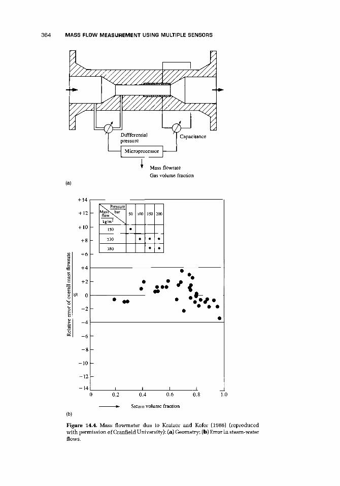
364 MASS FLOW MEASUREMENT USING MULTIPLE SENSORS
(a)
+ 14
+ 12
+ 10
+ 8
+6
+4
+2
t$ 0
2
- 4
- 6
- 8
- 1 0
-12
- 1 4
(b)
Mass flowrateGas volume fraction
-
—
_
N^ PressureMasSv barflow \kg/m2 ^ ^
150
230
380
50
•
-
• • •
1 1
1 1
100
•
150
•
•
200
•
•
• * • • • * < f
••
1 1 10.2 0.4 0.6
» Steam volume fraction
0.8 1.0
Figure 14.4. Mass flowmeter due to Kratzer and Kefer (1988) (reproducedwith permission of Cranfield University): (a) Geometry; (b) Error in steam-waterflows.

14.4 MULTIPLE SENSOR METERS FOR MULTIPHASE FLOWS 365
multiphase flowmeter, particularly for oil well flows, but it would be necessary forthe continuous phase to be conducting.
14.4 .3 MULTIPHASE METERING FOR OIL PRODUCTION
The following list, which uses Dykesteen;s (1992) categorization, is a compilationfrom papers by King (1990), Whitaker (1993), Whitaker and Millington (1993), andothers (cf. Kjolberg and Berentsen 1997, who tested five meters from Fluenta, Framo,ISA, Kvaerner, and MFI, and Klemp et al. 1997 on field developments).
Separation of ComponentsThe Texaco SMS subsea metering system (Figure 14.5) combines an inclined gravityseparator, a microwave sensor in a side stream sampling loop for water cut, a dif-ferential pressure liquid flow rate meter, a vortex-shedding meter on the gas outlet,and temperature and pressure measurements (cf. Dean et al. 1990a, 1990b).
Measurement of the Multiphase Flow Rate, but Separation of a Samplefor Component MeasurementSome early results were reported by Hall and Shaw (1988) and were for a multiphaseflowmeter on the Rolf facility in the Danish section of the North Sea. This systemdepended on turbine meter, gamma densitometer, pressure, temperature, and flowseparation. Typical error values for favorable conditions were 25 %, but some very se-vere errors were recorded in the water measurements. A commercial device similar tothis claimed pipe size up to about 600 mm, pressure up to about 65 bar, temperatureup to 400°C, and flows up to about 8,000 m3/h.
A system was reported (Anon. 1988, Kinghorn 1988) using a correlation flowme-ter and gamma densitometer to monitor the main flow after jet mixing and took
Inclined separatorsection Pressure
transducerGas temperaturetransducer
Liquiddensitometer
Outlet(multiphase flow)
Figure 14.5. Subsea metering system (Dean et al. 1990a; reproduced with permission from theNEL).

366 MASS FLOW MEASUREMENT USING MULTIPLE SENSORS
a sample of the flow, separated the liquid and gas components in the sample andmeasured the water content of the liquid component (cf. King 1988; Millington andKing 1988, who used a jet mixer/turbine meter package).
S. G. S. Redwood (published reports appear to associate this development withNEL and Imperial College, London, England) used a static mixer, with venturi orpressure loss across the mixer, for total flow rate. Density was obtained with a gammadensitometer at the venturi throat. In addition, a small sample of the mixture wasextracted and separated, and a Coriolis meter was used to obtain the water cut (Anon.1994). King (1988) also mentioned the use of ultrasonic cross correlation (cf. Sidneyet al. 1988a, 1988b).
Tuss (1996) described tests of an Agar multiphase meter consisting of a positivedisplacement meter to measure the total volume of the flowing stream, a venturi tubeto measure gas liquid flow rates, and a water cut monitor to measure water-liquidfraction. A gas bypass loop measures the gas volume flow. About 10% uncertaintyof the reading for each component appears to be claimed.
In-Line Measurement of All ParametersFluenta, with work from the Christian Michelson Institute (Dykesteen et al. 1985),developed a meter. It obtained the velocity from cross correlation of signals fromspaced capacitance sensors and used these sensors with gamma densitometer toobtain the makeup of the fluid. The velocities of all the components were assumedto be equal (cf. Frantzen and Dykesteen 1990). The Fluenta MPFM 900 is a full-bore, noninvasive instrument using capacitance to determine the water cut and theaddition of gamma ray absorption to obtain phase fractions (Millington et al. 1993).The flow rates are obtained from cross correlation of the axially spaced capacitancesensors with measures of large and small bubble transits.
Torkildsen and Hanssen (1996) described the Framo meter as consisting of
• static flow mixer for homogenizing the flow;• multi energy gamma meter for measurement of the oil, water, and gas fractions;
and• venturi meter for measurement of the total flow with differential pressure, pres-
sure, and temperature transmitters.
Torkildsen et al. (1997) commented on the need to be aware of the possibilitythat flow regime and salinity may affect the meter performance.
The ISA Controls/BP meter (Priddy 1994) (Figure 9.21) uses a twin helical screwpositive displacement meter with gamma density meter spanning the flow betweenthe two sets of screws.
The CSIRO, Australia, developed a multiphase meter based on gamma rays toobtain mass, cross correlation of gammas to obtain velocity and dual-energy gam-mas to obtain mass fraction of oil in liquid. In addition, pressure and temperaturemeasurements were made, and specific gravities, etc., of the components were known(Watt 1993). A measurement uncertainty of between 5 and 9% appears to have beenachieved.
14.5 CHAPTER CONCLUSIONS 367
The Kongsberg/Shell meter uses capacitance to obtain the gas-liquid interface inthe channel, the oil-water fraction, and, by cross correlation, the slug velocity andto estimate the individual flow rates.
The Multi-Fluid International (MFI) meter is suitable for flows with continuousoil component. The composition is obtained with microwave and gamma radiation,and velocity is measured using cross correlation between two dielectric sensing sec-tions. Okland and Berentsen (1994) described tests of the MFI, which suggested thatafter optimization the MFI could achieve uncertainty on oil flow rate within 5%.
Using a combination of venturi, capacitor, and single-beam gamma densitome-ter, Fischer (1994) showed that, provided the mixture was homogeneous, the massflow rates of the components of oil-water-air could be obtained within about ±25%.
Another method that has been looked at is pulsed neutron techniques (Anon.1993). Ekrann et al. (1988) included flow measurement as part of a capacitive systempresumably by using a correlation method.
The trend appears to be toward a meter that allows full-bore measurement ofall components, although removal of a small sample may allow a higher precisionwhile the technology develops.
Whitaker and Millington (1993) concluded that, from available evidence, thethen state of the art should have allowed phase flow rates to be measured to ap-proximately 10% over reasonably wide operating envelopes. Whitaker (1993) alsoappeared to conclude that 10% or so bulk measurement uncertainty was unlikely tobe bettered without new technologies and more recently (Whitaker 1996) confirmedthe ±10% of reading for four meters: Agar, Fluenta, Framo, and MFI.
See also North Sea Flow Measurement Workshops 1992, 1993, and 1994 for fur-ther papers on multiphase flow meters and mixers.
14.5 CHAPTER CONCLUSIONS
This chapter has been concerned with a wide range of mass flow measurementthat falls outside the meters discussed in Chapters 15-17. Apart from the hydraulicWheatstone bridge method that has had a particular market niche, the other multi-meter methods are likely to be in competition with the increasingly versatile Coriolismeter. The most promising multimeter development is likely to include ultrasonics.
It is in the area of multiphase flows that the major developments are likely to oc-cur, backed by the considerable cost advantages that result from subsea multiphaseflow measurement. These are likely to have improved component ratio measure-ment and clever data handling to obtain the most information. We shall, therefore,concentrate on these, always remembering that other areas of industry beyond theoil industry will benefit from such developments.
14 .5 .1 WHAT TO MEASURE IF THE FLOW IS MIXED
It would be satisfactory to have a flowmeter that could interpret all the variables thatoccur in a multicomponent flow. Such a device might identify the position on a flowpattern chart for well-documented fluids. It could also deduce the mass flow of eachcomponent. The state of the art has not reached that point yet, and it is likely to be
368 MASS FLOW MEASUREMENT USING MULTIPLE SENSORS
several years before it does. It is therefore important to consider what variable weare seeking in the measurements that are being made now. The most useful measureis clearly mass flow of the separate components. But the sophistication needed toachieve this for gases and liquids, without errors due to water, sand, and wax, ishigh, and most methods will need to compromise.
Beg and Toral (1993) reported on the use of pattern recognition techniques toobtain superficial gas-liquid flow rates. They reckoned that the techniques could beextended to oil-water-gas flows by using pressure sensing and an orifice plate withcapacitance and gamma ray. They introduced a new hydrodynamic system for scal-ing pipe diameter and fluid properties and used neural network pattern recognitiontechniques (cf. Toral et al.'s 1990 computer package).
The use of mixing to create an almost homogeneous flow also has drawbacks.The flow downstream of a mixer is extremely disturbed, and such a position wouldcertainly not be recommended for precise conventional flow measurement. In manycases, the flow also starts to separate as soon as it is mixed. The flowmeter wouldneed to be calibrated in these flow conditions, and such a calibration would need totake account of the effect of varying component ratios. The possibility of using thepressure loss across the mixer was noted earlier.
14.5 .2 USABLE PHYSICAL EFFECTS FOR DENSITY MEASUREMENT
Because it is unlikely that direct mass flow measurement will be suitable for multi-phase flows, we need to consider the indirect measurements that could be combinedwith a flow rate measurement. These are
• weighing elements;• vibrating elements;• acoustic methods (sound speed, acoustic impedance);• electromagnetic field methods (magnetic resonance, electrical capacitance, static
charge); and• nuclear radiations (X-ray, microwave, gamma).
It becomes apparent that, for two-component flows, some of these are unsuitablebecause, for instance, bubbles and particles do not follow vibrating movements. Op-tical (transmission problems) and thermal (heat transfer across boundaries) methodshave not been listed because they, also, are unlikely to be suitable (cf. King 1990).
However, Dykesteen et al. (1985) suggested that the measurement of resistanceand capacitance could achieve multicomponent ratio measurement. One manufac-turer has offered a full-bore device for measuring water in oil from 0 to 80% usingcapacitance methods for pipe diameters up to 300 mm and with the possibility ofa ceramic-lined device for pressures above 16 bar. Microwaves are used by anothermanufacturer for the measurement of water in oil by absorption. Nucleonic mea-surement has also been offered commercially as part of a three-phase unit for oil,water, and gas. Frantzen and Dykesteen (1990) report a multiphase fraction metercombining capacitance and gamma radiation, which looks very promising. Gains-ford (1990) described meters to obtain water fraction in oil, as well as oil, water,and gas fractions. It appears that microwave or gamma radiation were used for theformer and a combination for the latter.

14.5 CHAPTER CONCLUSIONS 369
Work in Shell laboratories (van Santen et al. 1995) also suggested that dual-energy absorption techniques with gamma- or X-rays may offer an on-line moni-toring method for individual fractions of oil, water, and gas in pipelines but maybe subject to errors from change in water salinity and also possibly from changes indistribution in space and time.
14.5.3 SEPARATION OR MULTICOMPONENT METERINGThe problems relating to the accurate measurement of multicomponent flow areso great that separation has been the only viable route in most cases. Whetherseparation of the components continues to be used will depend on the followingconditions.
a. The components are separable. This may be difficult in truly two-phase fluidsand in fluids where the finished product contains several components such asliquid foods.
b. The environment is conducive to separation. Subsea separation may be moredifficult than multicomponent flow metering.
c. The ultimate level of accuracy required can be achieved without separation.d. A complete system for multicomponent flow, pumps, valves, etc., is available.
Separation of the components and subsequent measurement of each componentmay offer the quickest route to an accuracy that approaches fiscal requirements, butin the longer term competitive methods that do not separate may result from elegantapplications of more advanced physics and clever computational interpretation ofsignals.
14.5.4 CALIBRATIONNational Engineering Laboratory, Scotland, now has the facilities to test multiphaseflowmeters for hydrocarbon flows (cf. King 1990).
It is tempting to suggest, as for single-component calibration rigs, that the testsection of such a rig should be preceded by a long settling length to obtain fullydeveloped flow. However, there are good reasons why such an approach is less ap-propriate for a multicomponent rig.
i. The settling length may be impracticably long.ii. The orientation of the pipe will affect the flow, and a long settling length will
prohibit other than horizontal orientations.iii. It is virtually certain that actual installation positions will not have fully devel-
oped flow conditions.iv. The enormous range of flow conditions requires that the flowmeter accuracy is
not dependent on particular flow conditions.
A more appropriate design for such a rig is likely to be a test section preceded by ashort upstream section and a manifold for component injection. By selection of theinjection manifold, flow regimes could be constructed upstream of the flowmeter.The whole unit including manifold, upstream section, and test section would beshort enough to rotate to any orientation so that both horizontal and vertical flowscould be simulated. The outlet flow through a flexible pipe would enter a separator

370 MASS FLOW MEASUREMENT USING MULTIPLE SENSORS
before recirculation. Such a rig may also have a small enough total volume to allowlive crude to be used as one component for oil-related flows.
Other combinations of flow components for other industries may lend them-selves to other rigs using more conventional calibration methods such as volumeand mass measurements of the total flow passed.
See also Mazzoni et al. (1994) for a description of a multiphase test facility.
14.5.5 ACCURACYThe errors in the papers reviewed on multicomponent/multiphase flows range from±1 % for an ultrasonic correlation flowmeter in paper pulp flow, for example, to asmuch as 25% for one of the offshore oil flow measurement systems. This range oferror is symptomatic of the problem for the flowmeter designer. For control and dis-tribution, a measurement uncertainty of order ±10% may be acceptable. However,high accuracy is required for fiscal and custody transfer applications, and here thelevel that can be achieved by the designer is far from clear. Is even ±5 % achievablein multicomponent oil flow measurement?

CHAPTER 15
Thermal Flowmeters
15.1 INTRODUCTION
There are broadly two concepts of thermal flowmeter now available for gas massflow measurement, one of which is also applicable to liquids. I shall follow the use-ful terminology in ISO committee draft (ISO/CD 14511:1998) for the two types. Thefirst is the capillary thermal mass flowmeter (CTMF), which has broad applicationsin the control of low flows of clean gases, but which can also be used with a by-pass containing a laminar element to allow higher flow rates to be measured. Thearrangement of heaters and coils between the various manufacturers differs, but thebasic approach is the same, with heat added to the flowing stream and a temperatureimbalance being used to obtain the flow rate.
The second is the full-bore thermal mass flowmeter (ITMF), which is availableas both insertion probe and in-line type. It has a widely used counterpart in thehot-wire anemometer for measurement of local flow velocity, but, as the need for agas mass flowmeter has become evident, it has been developed as a robust insertionprobe for industrial usage and then as the sensing element in a spool piece flowmeter.It has been produced by an increasing number of manufacturers in recent years as asolution to the need for such a mass flowmeter.
15.2 CAPILLARY THERMAL MASS FLOWMETER - GASES
In various examples of the CTMF, the gas flows through a very small diameter tubethat has heating and temperature-measuring sensors. For larger flows, this is usedwith a bypass laminar flow element in the main gas stream. In many cases, themass flowmeter is in one unit with the control electronics and the gas control valve.However, in this chapter our interest is in the meter itself.
15.2 .1 DESCRIPTION OF OPERATION
In this design of thermal flowmeter, the gas flows through a very small diametertube, with a sufficient length-to-diameter ratio to ensure laminar flow, and on theoutside of which there are heating and temperature-sensing windings. The heaterwinding transfers heat through the wall of the tube to the gas. If there is a gas flow,the heated gas is carried downstream. The downstream temperature sensor will thensense a higher temperature than the upstream sensor. This differential can then beused to deduce the mass flow. A diagram is shown in Figure 15.1 (a). The equation
371

372 THERMAL FLOWMETERS
HEATER
(a)
(b)
TEMPERATURE^-SENSORS
HEATERS
(c)
(d)
LAMINAR FLOWBYPASS ELEMENT
Figure 15.1. Diagram to show the various configura-tions of CTMFs: (a) Central heater with upstream anddownstream temperature sensors; (b) Three heaterswith sensors to ensure that they remain at constanttemperature; (c) Two combined heaters and resis-tance thermometers; (d) One downstream heater withtwo sensors; (e) Bypass with laminar flow element.
for this is given in the steady state byqm = Qh/(KcvAT) (15.1)
where qm is the mass flow rate to be mea-sured in kilograms per second, Qh is theheat input in Joules per second, K is a con-stant, cp is the specific heat at constant pres-sure in Joules per kilogram Kelvin, and ATis the measured temperature difference inKelvins. A knowledge of K, Qh, and cp al-lows qm to be deduced from AT.
In an alternative mode of operation [Fig-ure 15.1(b)], the sensed temperature is usedto adjust the heat into three heaters to keepthem at a constant temperature. The energyrequired in this mode to restore equilibriumto the windings can be used to obtain theinstantaneous rate of flow. This results in asensor with a short response time.
Figure 15.1(c) shows a design that usesthe temperature difference between twocoils positioned along the tube axis, bothof which are heated. The coils also act as re-sistance thermometers. When flow occurs,the downstream coil is cooled less than theupstream coil, and the differential temper-ature is used as a measure of the flow.
Figure 15.1(d) shows a design with twotemperature-sensing coils and one heatercoil.
In order to accommodate a greater flowrate than is possible through the capillary, alaminar flow bypass is used [Figure 15.1(e)].The total flow rate through capillary and
bypass is then proportional to the flow through the capillary. In some designs, acontrol valve is incorporated. In others, an air-actuated valve may also be offered bythe manufacturer.
Figure 15.2 shows an industrial CTMF with bypass through n identical elements,where n can be selected for the appropriate flow range. It also shows the valve,operated from a second amplifier, which controls the flow.
In another design [Figure 15.3(a)], the means of heating the tube is through acurrent passed along the tube wall, which, in turn, heats the fluid. Two heat sinks,one at each end, conduct away the heat that has passed up the tube. The fluid coolsthe tube, and the resultant temperature difference is measured in two places withthe thermocouples TCi and TC2; the flow rate can be deduced from the difference.As with the other designs of thermal flowmeter, this one can be used with a by-pass. The distributions of temperature for zero flow and for a small flow are shownin Figure 15.3(b). It can be seen that the temperature difference between the two

15.2 CAPILLARY THERMAL MASS FLOWMETER - GASES 373
SENSOR TUBE(CAPILLARY}
R,
wwwwwwwwwww
^\\\\\\\\3(\\\\\\\\\\\\\M\v
OUTPUT
EXTERNALCONTROL
FT -- nf
L BYPASS DIVERTS SMALL PERCENTAGE OF GAS FLOWTHROUGH SENSOR (CAPILLARY) TUBE.
Figure 15.2. Industrial capillary thermal mass flowmeter showing schematic of flow paths andelectrical diagram (reproduced with permission of BOC Edwards).
thermocouples will be zero at zero flow but will increase with flow. The equationderived for this flowmeter is reproduced by Hemp (1995a) (cf. Appendix 15.A.4).
All these varieties are dependent on a knowledge of cp, which depends on thegas and varies with pressure as shown in Table 15.1.
HEATSINK
FLOW
t-TC,
- ELECTRIC •CURRENT
•e-(a)
HEATSINK
TC,
• \
Figure 15.3. Heated tube thermal flow-meter (after Hastings): (a) Schematicdiagram; (b) Temperature distributionunder static and flowing conditions.
NO FLOWTEMPERATURE
HEATSINK
(b)
FLOW
TC?
DISTANCE^ ALONG
HEAT T UBESINK

Table 15.1. Variation of cp with pressurefor four gases
Gas
H2Airo2CH4
Approximate % Variation0-10 bar
+0.1+2+1+2
40-100 bar
+1.6+16+18+31
374 THERMAL FLOWMETERS
It is important for the calibration of themeter to be close to, or referenced to, oper-ating conditions; otherwise, it will be nec-essary to look up the data for the gas andpressure at operation. Temperature varia-tion has only a slight effect on the value ofcp. For example, for air it is 0.01%/°C, andfor methane it is 0.11%/°C. Viscosity vari-ation has a negligible effect unless the gasis near liquefaction. Calibration may be ref-erenced to primary volumetric standards at
atmospheric conditions and corrected normal temperature and pressure or standardtemperature and pressure.
15.2.2 OPERATING RANGES AND MATERIALSFOR INDUSTRIAL DESIGNS
Rangeability is up to 50:1. Flow ranges are from 0 to 3 ml/min or lower to 0-1001/min or even up to 1,000 m3/h for special bypass designs. A 100-mm diameter meterwould typically give a range up to about 250 m3/h and a 200-mm diameter meter upto about 1,000 m3/h. Note that, for air at ambient conditions, 1,000 m3 has a massof about 1.2 kg.
These meters may be able to operate for some designs up to about 200 bar oreven, in some cases, 300 bar pressure. Temperature operating range may be 0-65°Cwith a coefficient of less than 0.1%/°C. Pressure drop on the line is up to 0.02 barfor the maximum flow rate.
Materials in contact with the gas include 316, 316L, and high alloy ferriticstainless steel; anodized aluminum, brass, and Viton; Buna-N; Kalrez; and Teflonor silicone O-rings.
Power supply requirements usually relate to 15 and 24 V DC versions; whencombined with a controller, these may draw up to about 180 mA resulting in powerconsumption of order 3.5 W.
Flowmeters are likely to be factory-set to a preselected gas, pressure, and flowrange. Correction factors range from about 0.55 for ethane to about 1.40 for argonagainst air. These may also be referred to nitrogen.
15.2.3 ACCURACYUncertainty is typically claimed as ±1% full-scale deflection or FSD (or for a recentdesign ±0.75% rate ±0.25% FSD) but may be ±1.5% for the top end of the flowrange and ±4% FSD in some other cases, depending on design and the temperatureand pressure range. Repeatability is typically 0.2-0.5% FSD, but in some cases it maybe quoted as being of order ±0.25% of rate and in at least one case as 0.05% FSD. Inaddition, there may be pressure and temperature coefficients.
15.2.4 RESPONSE TIMEAn exponential curve is usually used to indicate the response of a flowmeter. Theexponential curve is given by
5 = 50(l - e~t/T)

15.2 CAPILLARY THERMAL MASS FLOWMETER - GASES 375
To Approach Within
5%2%1%0.5%
Response Time
3T
4r4.6r5.3r
The time constant x gives the time for £v'^ " ' "1^ i : i"v"4 ' ^ - ^ >,/ ,^ ,, ,^,^, «.*the flow signal 5 to reach about 60% of its I Table 15.2. Time to approach the finalfinal value So. Table 15.2 gives the times to i v a l u e a f t e r a flow changeapproach the final value.
T is of order 250 ms to over 1 s. A stan-dard instrument may take 1-5 s to settleto within 2% of final value for a 0-100%command change. However, manufacturersmay claim a response of about 1 s for some . . ^ - < - . < , ,designs.
Thermal drift may be reduced against ambient temperature changes by insu-lating the unit, but with the consequence of a longer time constant (Sullivanno date). A solution is to enclose the sensor in a temperature-controlled envi-ronment. Sensors may also suffer from radiofrequency interference and may beincompatible with corrosive gases. Typically, a 30-min warm-up time may beneeded.
15.2.5 INSTALLATIONThere is unlikely to be any effect from upstream pipework for the basic device with-out bypass because the bore of the tube is so small that the profile will be readjustedbefore reaching the elements. For bypass designs, there may be an effect, and itmay be necessary to include 20D upstream straight pipe (Gray et al. 1991). Designsshould ensure that flow is truly laminar in the bypass, by suitable matching of sizeand pressure drop.
There may be significant effects on sensitivity that can seriously impair accu-racy under certain conditions of installation (e.g., mounting angle), gas density, andpressure when outside normal operating envelopes. Zero offset appears to be affectedby meter orientation and may result from free convection when the meter is nearvertical. Rarefied gas flows may also create problems.
Temperature effects on meter zero are up to 0.15% FSD/°C and on span are lessthan ± 1 % FSD over a 10-50°C range. Pressure sensitivity is of order ±0.4% per barup to about 14 bar. Power supply sensitivity is of order ±0.1% FSD per percent powersupply voltage variation.
Typical weight is of order 0.5-2.5 kg. For bypass designs, the weight may beup to 20 kg. Meters should have been subjected to burn-in and cycling prior toshipment.
Gray et al. (1991) discussed environmental factors that affect mass flow con-trollers (MFC). The MFC is tested with a vacuum diagnostic system to which theMFC is connected. The test chamber is evacuated to below 50 mtorr, and the valveto the vacuum pump is then shut. The initial flow rate is set, and the pressure is mea-sured as it rises. From this, the time to achieve controlled flow, actual flow rate, error,and deviations from flow are obtained. They tested various effects and concludedthat, to minimize effects, temperature extremes must be avoided and surroundingsshould not be allowed to raise the temperature of the gas boxes, pressure shouldbe carefully regulated, and vibration should be avoided. Where possible, tubing dis-tances should be minimized, and MFCs should be mounted in a normal uprightorientation.

376 THERMAL FLOWMETERS
15.2.6 APPLICATIONSCTMFs are most commonly applied to low flows of clean dry gases above their dew-points (e.g., gas blending, semiconductor industry). Gases quoted by manufacturersinclude air, acetylene, ammonia, argon, arsine, nitrogen, butane, carbon dioxide,carbon monoxide, chlorine, ethane, ethylene, fluorine, Freon 11, Freon 12, Freon13, helium, hydrogen, hydrogen sulfide, krypton, methane, neon, nitrous oxide,oxygen, propane, propylene, silane, and xenon. Examples of problem gases thathave been used with this type of meter include
• BCI3 (boron trichloride) corrosive gas;• SiCU (silicon tetrachloride) corrosive and low vapor pressure gas;• CCI4 (carbon tetrachloride) low vapor pressure gas;• SiH4 (silane) typical of gases that react and create deposits, resulting in clogging
of flow controllers; and• WF6 (tungsten hexafluoride) similar to the handling problems of silane.
The meter may be used with a wide range of gases for processes involving crystalgrowth, thermal oxide, diffusion, chemical vapor deposition, sputtering, ion im-plantation, and plasma etching, and the gases involved will each require a correc-tion factor against the calibration gas, possibly nitrogen, which may vary betweenas low as 0.17 for Freon-C318 (C4F8) or perfluoropropane, and as high as 1.543 forkrypton. The manufacturer should be asked for the compatibility of any particulargas and the correction factor (Sullivan no date). In selecting a flowmeter, particularcare should be taken where the inlet pressure is less than atmospheric or has a vaporpressure less than atmospheric.
15.3 CALIBRATION OF VERY LOW FLOW RATES
One method of calibration of these flowmeters for low flow rates is by means of aspecial piston proven A piston moves within a precision glass tube. The piston isconnected to a counterweight by means of a tape that turns an encoder wheel. Thetemperature and pressure of the gas are measured while flow is taking place.
Positive displacement devices or piston meters may achieve calibration to anaccuracy of about 0.2% of reading over a range from 0.02 to 30 l/min (Sullivan et al.no date). The volume flow at standard temperature and pressure (STP), subscript s,may be obtained from the actual, subscript a, using
Zpa_va Ta ps
15.4 THERMAL MASS FLOWMETER - LIQUIDS
15.4.1 OPERATIONThe diagram in Figure 15.4 shows the layout of a meter with parallel tubes runningbetween a heating block and a heat-sink block. At the midpoint of each tube is the

15.4 THERMAL MASS FLOWMETER - LIQUIDS 377
Body(Heatsink) I
IInterface -1
AI-Tidy
Sensor zone 2B T 4
Sensor zone 1
—i
1>J
Ttop
Guideline
—
HTop
(Heater)Process wetted
part316LSSTtop - Tbody = (20°C for Model 5881,10°C for Model 5882).
Figure 15.4. Liquid mass flowmeter (reproduced with permission from FisherRosemount Ltd.).
temperature sensor. The heating causes an increase in temperature of 10 or 20°C.When the flow takes place, heat is converted, and the difference between T3 and T4
will vary with the mass flow rate. It appears that the heat is then conducted throughthe body of the meter. The liquid may increase in temperature by as much as 15°Cwithin the meter, but there is negligible change in liquid temperature outside thedevice.
Huijsing et al. (1988) described a new meter aimed at fuel consumption mea-surement in automobiles and light aircraft and also industrial processes. The ex-ternal muffs (for heat transfer and temperature measurement) of other designswere replaced with internal copper blocks, perforated with multiple axial holesthrough which the liquid flowed, resulting in much greater thermal contact with theliquid.
15.4 .2 TYPICAL OPERATING RANGES AND MATERIALSFOR INDUSTRIAL DESIGNS
For liquids, minimum measurable flow is about 0.002 kg/h with a maximum mea-surable flow of between 0.1 and 0.5 kg/h, depending on the design, and a turndownof up to about 15:1. Accuracy is about 0.5-1% FSD and repeatability 0.2% of rate forthe upper end of the range and 0.1% FSD for the lower part of the range. Repeatabilityis of the order of ±0.5% FSD per month.
A bypass arrangement allows greatly increased flow range up to 100 kg/h, butthe measurement uncertainty is likely to increase to about 2% FSD. However, ifextreme range turndown ratios are claimed, it is likely that the manufacturer willgive a performance envelope for the meter.
The ambient temperature range may be from 0 to 65°C, and pressure ratingscan be as high as 400 bar. Maximum viscosity may be about 100 cP. Pressure loss atoperating conditions is claimed as very small.
The response time for sensors is likely to range from 0.5 s up to about 10 s forthe largest meters, but the response for controllers should be obtained from themanufacturer.

378 THERMAL FLOWMETERS
15.4.3 INSTALLATION
Pipe size connections range from ^ to \ in. (about 1.5-6 mm) with materials ofstainless steel and seals of Buna-N, Viton, PTFE, or Kalrez. Process temperature changecan cause +0.02%/°C, and ambient temperature effects can cause up to +0.03%/°C.
15.4.4 APPLICATIONS
It may be suitable for measurement of very low flow rates of toxic, corrosive,and volatile liquids (liquefied gases under pressure), catalysts in petrochemicals,pigments in paints, reagents in pharmaceuticals, flavorants, enzymes, antibioticsin food, odorants into natural gas, titanium chloride closing into furnaces for hard-ening metals, corrosion inhibitors in pipes, and reagents in fermenters. It also mayoffer a means for controlling and measuring very low flows in laboratories con-cerned with microfiltration, measurement of porosity of rocks, fuel consumption,lubrication, gas/vapor mixtures, and chromatograph flows, as well as controlling theinjection of additives (catalyzers) into industrial reactors.
15.5 INSERTION AND IN-LINE THERMAL MASS FLOWMETERS
The in-line thermal mass flowmeters (ITMFs) represent an alternative design conceptto the CTMF, and both insertion and in-line versions appear to be aimed at the samegoal - mass flow measurement of gases in pipes and ducts.
In Figure 15.5 there is a diagram of an arrangement for an ITMF. The heaters andtemperature sensors for either insertion or in-line designs may be contained in oneor two probes, may use the same element for both functions, and, where two probesare used, will often, as in Figure 15.6, be in the same cross-section of the duct.
This flowmeter (Kurz 1992) uses a heated element in a flowing stream, theconvective heat transfer of which is dependent on the temperature difference be-tween the probe and the fluid, on the flow rate, and on characteristics of thefluid. A second temperature probe is used to measure the temperature of the fluid.Two types have been used: the constant power and the constant temperatureanemometers. The temperature of the heated probe in the former varies with fluidvelocity and is used as the sensing parameter. The response is slow due to the ther-
mal inertia of the probe, and the zero is un-stable because natural convection becomesimportant at low flows. In the latter type,the probe is kept at constant temperaturethrough a feedback control circuit, and thepower needed to retain this constant tem-perature is used to obtain the velocity. As aresult, the response is much faster, typically1 s for a 67% change. The resistance of thesensing elements is connected into a modi-fied Wheatstone bridge (Figure 15.6, cf. Fig-ure 15.A.I), in which the voltage across thebridge is amplified and fed to the top of the
HEATERS &SENSORS
Figure 15.5. Diagram of an ITMF with either inser-tion probes or in-line design. In the latter, the probesare often in the same cross-section.

15.5 INSERTION AND IN-LINE THERMAL MASS FLOWMETERS 379
RESISTORS
SENSOR
Figure 15.6. Schematic of in-line thermal mass flowmeter showing Wheatstonebridge arrangement.
bridge to retain a constant temperature difference. By using a three-wire sensor, thelead resistance can also be compensated for.
The relationship for these flowmeters, from Equation (15.A.8), is
(15.2)
where qm is the mass flow rate, q^ is the heat supplied, and AT is the temperaturedifference between heated and unheated probes, k' is a constant that allows for heattransfer and temperature difference at zero flow, and K is a constant incorporatingthe area of the duct into which the probe is inserted, as well as gas and heat transferconstants. In Equation (15.A.8), n was equal to \. This may be approximately correctfor low velocities but may be more like \ for higher velocities. Factors affecting theequation, as well as free convection at low velocities, are some heat transfer fromthe probe to its base, usually small, and thermal radiation, which is small comparedto forced convection for normal temperatures.
15 .5 .1 INSERTION THERMAL MASS FLOWMETER
An example of an ITMF is shown in Figure 15.7(a) and consists of two pairs ofelements. In each pair, there is a resistance thermometer; coupled to these are, inone pair, a heated rod and, in the other, a similar unheated body as a mass equalizer.Flow past the heated element results in a heat loss, and the combination of this andthe differential temperature allows the flow rate to be deduced.
Insertion probes may be inserted into and withdrawn, without process shut-down, from a pipeline of 30- to 500-mm diameter. They may also be available withmultiple sensors for installation across a pipe [Figure 15.7(b)].

3 8 0 THERMAL FLOWMETERS
SENSORTHERMAL FOR GASMASS TEMPERATURE
HEATER SENSORSECTION A-A
(b)
Figure 15.7. Diagrams of single- or multisensor probe: (a) Showing individualsensor; (b) Showing multisensor probe in a pipe (after the design of FCI).
The uncertainty may be quoted, typically, as being of order ±1% FSD or ±3%rate, whichever is less, for turndown ratios of order 10:1. However, gas velocities upto about 60 m/s or more have been claimed with turndown up to 800:1. Manufac-turers who claim wider turndowns will presumably provide a calibration that relatesuncertainty to various points in the characteristic.
Various designs of these meters have been used for boiler applications (preheaterand combustion air), combustion gas flows, hydrogen coolant flow, gas pipelinetransmission flows, methane flows, nitrogen purges, flare gas flow, ventilation, heat-ing and air conditioning, and superheated and dry saturated steam.
Lai et al. (1991) discussed the use of thermal mass air-flow sensors (essentiallya hot-wire anemometer) for measuring the air flow into gasoline engines. A recom-mended arrangement is to have the mass air-flow sensors in a bypass of the intakeair passage of an engine. Possible errors may arise due to variation in the profile atinlet caused by filter blockage.

15.5 INSERTION AND IN-LINE THERMAL MASS FLOWMETERS 381
15.5.2 IN-LINE THERMALMASS FLOWMETERFigure 15.8 shows a commercial ITMFwith heated and unheated temperature-dependent resistors. Another approach thatmay be available uses two stainless steelwires in the flow stream in the throat ofthe transducer - one heated with a current,and a bridge circuit to adjust the current tokeep the temperature between them, mea-sured by their resistances, constant. Theremay also be designs that heat the fluidand sense its temperature from outside thetube, leaving an unobstructed bore to thetube.
15.5.3 RANGE AND ACCURACYMeters of 25-200 mm may be availableas flanged or, in some sizes, as wafer de-signs. Turndown is of order 50:1 or higherwith uncertainty of 2% of rate and within aband of order 4% down to 1% FSD. Uncer-tainty may be quoted in the range ±1.5%to ±2.5% FSD. Repeatability may be givenas 0.25-3% of rate or as 0.25-1% FSD, thelesser value being taken. The manufacturers give correction factors for variousgases.
Flow ranges are from 2-125 kg/h to 300-8,000 kg/h or greater. Response time isabout 0.2 s. Pressure drop is up to 10 mbar. Operating pressure is up to 40 bar. Thetemperature range is —50 to 300°C or greater, depending on the design. Hygienicversions are available. There may also be temperature effects of order ±0.3% rate or±0.08% FSD/°C.
Figure 15.8. Photograph of an in-line thermal massflowmeter (reproduced with permission from Endressand Hauser).
15.5.4 MATERIALSMaterials of construction are typically stainless steel with seals of Viton rubber andencapsulated sensor elements, consisting of platinum resistance thermometers orthermistors, in stainless steel or glass.
15.5.5 INSTALLATIONInstallation orientation may affect the performance, and manufacturers' instructionsshould be followed. Installation requirements recommended by one manufacturerare given in Table 15.3. For a flow conditioner of the perforated plate type basedon the Mitsubishi design, this manufacturer recommended 8D upstream spacingwith wafer and insertion-type meters, and with larger in-line meters, but allowedpositioning of the flow conditioner at the inlet flange of the in-line design for

382 THERMAL FLOWMETERS
Table 15.3. Installation requirements for a wafer or insertion thermalmass flowmeter compared with those for a f$ = 0.55 orifice plate (afterEndress and Hauser)
Upstream Fitting
90° bend or T-piece2 x 90° bends same
plane2 x 90° bends
perpendicular planesReducerExpanderControl valve
Thermal
Upstream0
20D25D
40D
20D20D50D
Flowmeter
Downstream^
5D5D
5D
5D5D5D
Orifice Plate (/3 = 0.55)
Upstream
16D22D
44D
8D20D24DC
Downstream
6D6D
6D
6D6D6D
Note: Upstream distances should be doubled for light gases such as helium and hydro-gen.a Reduce by about 5D for flanged in-line flowmeter.b Reduce by about 3D for flanged in-line flowmeter.0 Globe valve fully open.
25- to 100-mm diameters. The manufacturer reckoned that, for a control valvedownstream, there should be 10D separation (8D to flange of in-line flowmeter).Gaskets, flanges, and pipes should be correctly sized and aligned. The table com-pares the ITMF with a /3 = 0.55 orifice plate and shows that the requirements areabout the same apart from the reducer and the valve (not recommended upstream),which are more stringent for the ITMF. For the in-line version, the agreement is evencloser.
The influence of temperature variation can be as small as 0.05%/K rate and ofpressure 0.2%/bar rate.
15.5 .6 APPLICATIONS
This may be an alternative meter for installations where orifice or vortex me-ters are commonly used for gas mass metering. Examples are chemical engi-neering and processing technology, semiconductor process gas measurement andcontrol, combustion air measurement for large utility plant, mass flow rate forstack effluent, air sampling in nuclear plant and environmental facilities (Kurz1992), flare gas systems, leak detection, food industry (e.g., CO2 metering inbreweries), internal works gas consumption measurement, dosing plants, nitro-gen and oxygen flows in steel works, burner control, combustion and pre-heated air, flue gas, methane, moist and corrosive gas from sludge digester,compressed air in hospitals and other medical applications, argon and heliumflows in laboratory environments, waste air measurement, and large ducts. Thesemeters are unlikely to be suitable for steam, but the manufacturer should beconsulted.

15.6 CHAPTER CONCLUSIONS 383
Haga et al. (1995) used a thermal flowmeter for fuel vapor flow measurementand used electrical heaters to ensure that the piping was of a temperature to preventliquefaction of the vapor. A liquid recovery container and a filter were provided atthe inlet of the flowmeter. To prevent the remaining vapor in the piping from beingliquefied, air purge was used. They gave expressions for specific heat and density asa function of pressure, temperature, and vapor pressure. Haga et al. claimed that ithad been possible to measure the vapor flow in real time for a moving vehicle andthat it offered a practical meter.
15.6 CHAPTER CONCLUSIONS
This technology, which is of more modest price than the Coriolis, is likely to beexploited because it also (with ultrasonics) offers a means of mass flow measurementand possibly greater versatility for gases. Development could take place in variousdirections:
• improved theoretical understanding and design of the CTMF to minimize pres-sure, temperature, and installation effects and to improve accuracy;
• further analysis of the ITMF designs to understand accuracy limitations, envi-ronmental, and flow profile effects (it should be remembered that the accuracyof this instrument depends in part on the measurement of a small temperaturedifference within a gas of variable temperature);
• improved theoretical predictions of a meter which is insensitive to flow profile(Hemp 1994a/5a);
• use of multiple probes;• use of nonintrusive heating and temperature measurement; and• self-checking with transit time to downstream probes.
Casperson (1993) described a device that used a thermocouple in a pulsed mode.Current pulses heat and cool the junctions, and the subsequent decay is monitored.With flow, the time constant will change. Being nonlinear, the device needed cali-bration.
An important development is microthermal sensors, which allow fabrication ofair-flow sensors as well as signal-conditioning electronics on a single chip (van Dijkand Huijsing 1995) with a standardized digital output signal for a microprocessor.The one described is direction-sensitive.
Nguyen and Kiehnscherf (1995) described a flow sensor in which the channelwith an area of 0.6 mm2 and length 10 mm was etched, and the sensor containedpolysilicon heaters and measurement resistances on the chip. The chip is bonded toPyrex glass to complete the channel. Four modes of operation were built into theelectronics to allow constant temperature and constant power operation. In this way,they tested with both liquid (0-500 ml/min or 0-10 ml/min) and gas (0-500 ml/min)(Figure 21.2).
With such standardized components, the possibility of bypass metering withmultiple and replaceable bypass meters is an interesting development.

384 THERMAL FLOWMETERS
APPENDIX 15. A
Mathematical Background to the ThermalMass Flowmeters
15.A.1 DIMENSIONAL ANALYSIS APPLIED TO HEAT TRANSFER
The heat flux density (Kay and Nedderman 1974) is given by
qh = f(AT, k, cp, p, ti, D, V) (15.A.1)
where AT is the temperature difference between the heat source and the fluid, k isthe thermal conductivity of the fluid, cp is the specific heat at constant pressure, pis the fluid density, \± is the dynamic viscosity of the fluid, D is the pipe diameter,and V is the fluid velocity.
One simple form of Equation (15.A.1) for CTMFs is
Qh = KATcpqm (15.A.2)
where Qh is the total heat input into the winding, and a knowledge of K, AT, andcp allow qm to be deduced.
We can identify dimensionless groups, which must have a functional relation-ship with each other. For this purpose, a number of heat transfer groups have beensuggested
Nusselt number (Nu) = ^ - (15.A.3)kAT
is the ratio of heat transfer to the rate at which heat would be conducted throughthe fluid under a temperature gradient AT/d;
Prandtl number (Pr) = ^ (15.A.4)K
is the ratio of kinematic viscosity to thermal diffusivity;
Reynolds number (Re) = - — (15.A.5)/X
is the ratio of inertia forces to viscous forces in the flow.These give a general relationship for heat transfer:
Nu = f(Pr, Re) (15.A.6)
A special case of this equation is that due to King for the hot-wire anemometer:
Nu = A + EPr° 5Re°5 (15.A.7)
where A = 1/n and B = (2/TT)0-5. The hot-wire or hot-film anemometer provides atool for the measurement of local fluid velocity.

15.A.2 BASIC THEORY OF ITMFS 385
15.A.2 BASIC THEORY OF ITMFs
King (1914) investigated the relationship between heat transfer rate and flow veloc-ity. Using Equation (15.A.7), the following expression gives heat loss per unit lengthof a cylinder of diameter d at a temperature of AT above the fluid temperature inwhich it is immersed:
qh = kAT+(27tkcvpdV)°-5AT (15.A.8)
where k is the thermal conductivity of the fluid, cv is the specific heat of the fluid atconstant pressure, p is the density, and V is the velocity assumed to be perpendicularto the cylinder (cf. Ower and Pankhurst 1966, who used cv in place of cp and alsoprovided details and early references).
As the velocity increases, the second term becomes more important, and the firstterm, which is due to conduction and natural convection, becomes more importantat very low flow rates. It is clear from this equation that it is necessary to measure q^and AT and hence to obtain V assuming that the constants of the wire and the fluidare known. However, the relationship between q^ and AT is more usually obtainedby calibration.
This, in turn, suggests that any device designed to measure velocity from thisformula will need a means of measuring the temperature of the stream as well as theheat loss from a heated wire. This may be achieved by calibrating the probe for theproposed application.
The other important observation is that, when the density is not constant, thecombination of velocity and density with the area of the meter will give mass flowrate.
King showed that in air the formula held down to a value of
Vd = 0.0187 (15.A.9)
where V is in centimeters per second, and d is in centimeters. At very low flow rates,the natural convection in the region of the wire becomes significant in comparisonwith the forced flow. Collis and Williams (1959) gave a Reynolds number, belowwhich convection becomes important, as
3 U5.A.H,,
where v is the kinematic viscosity, T is the ambient temperature of the air, and ATis the difference between the temperature of the wire and the ambient air.
Simplifying Equation (15.A.8) and introducing the heating current I through aresistance R, we can write
qh = I2R = C + DV0S (15.A.11)
where C and D are functions of temperature. But if the resistance of the wire orcylinder is kept constant, then the temperature of the wire or cylinder will also beconstant and so C and D will be constants of the meter for a particular fluid.
To maintain the constancy of the resistance, a bridge circuit such as that shownin Figure 15.A.I is used where the null indicator ensures that the resistances are all

386 THERMAL FLOWMETERS
ALTERNATIVE TO V
Figure 15.A.I. Constant temperature resistance circuit (after Ower andPankhurst 1966).
equal, and the current, and hence the power, is measured by means of the resis-tor in series with the bridge. The advantages of using a constant resistance com-pared with a constant current are that it is possible to maintain a constant tempera-ture and avoid thermal inertia, and that the equation is simplified as in Equation(15.A.11).
Using Equation (15.A.8) and allowing for temperature variation, we can rewriteit as
(15.A.12)
where K is a constant incorporating the area of the duct into which the probe isinserted and the gas and heat transfer constants, qm is mass flow rate, qh is heatsupplied, and AT is temperature difference between heated and unheated probes.
This provides the basic relationship for ITMFs with either ^ or AT constant.
15.A.3 GENERAL VECTOR EQUATION
The governing equation for flow with heat transfer under steady conditions is
kV - V T =
pcp pcv(15.A.13)
where qa is the added heat flux. This can be obtained from Hemp (1994a, Equations 2and 5)
qh = -kWT (15.A.14)

15.A.3 GENERAL VECTOR EQUATION 387
and
(15.A.15)
with the addition of the final term, which relates to the local heat addition. If allheat is added across boundaries with the flow, then the last term disappears. Hempuses Equations (15.A.14) and (15.A.15) to develop his weight function theory forthermal diffusion flowmeters. This is an elegant theory, and the interested reader isencouraged to refer to Hemp's papers. However, as he comments, the work at presentis probably mainly of theoretical interest.
We can write Equation (15.A. 13) for flow in a two-dimensional channel as
,= (dz pcv\dx2 dz2 pcv
(15.A.16)
We can simplify this for flow in a tube where we neglect temperature gradientsin any but the axial direction. Referring to Figure 15.A.2 and rewriting the gradientand the Laplacian as finite difference expressions, we obtain
v~ 2L L2 (15.A.17)
If we take the area of the duct to be A and the heat source to be at the center, whichhas a temperature Tc, we can rewrite the equation in terms of mass flow:
convectionterm
2kA (Ti - 2TC -
conductionterm
T2) 2LA+ -—^a (15.A.18)
heat inputterm
The first and last terms constitute the simplest approximation for the behavior ofthe thermal gas flowmeter. Heat is convected away by the flow, and the differenceof temperature between inlet and outlet is related to the heat input, the specificheat, and the mass flow. This assumes that the first term on the right-hand sidecan be neglected. However, in the case of no flow, the heat added is conductedaway, and the central term cannot be neglected because it gives the size of theconduction.
L L
7",
Figure 15.A.2. Diagram of tube to illustrate the use of finite differences.

388 THERMAL FLOWMETERS
15.A.4 HASTINGS FLOWMETER THEORY
Figure 15.A.3 shows the heat flows in the Hastings flowmeter based on an approx-imate one-dimensional theory. From the heat flows in the diagrams, we can derivethe simple equation of the meter. We consider first the wall, and specifically an ele-ment of length 8z. Here we have a heat addition as a result of the electric current /,which flows down the tube wall of resistance R per unit length. Thus the heat inputis I2R8z. From this element, heat flows along the wall, of amount <5Qh, which canbe related to the temperature gradient in the wall
Qh = -kA^- (15.A.19)
where A is the cross-section of the wall, and k is the thermal conductivity of the wallmaterial. Heat also flows out as heat loss from the meter, fiT, [i being a dimensionalconstant to give the heat loss based on the wall temperature, and it flows into thefluid, q±. From this we have an equation
(15.A.20)
ELECTRICCURRENT
IN
ELECTRIC ,CURRENT | /
OUTT±CENTER
FLOW LINE
\iThz
IELECTRICCURRENT•
HEAT FLOWSIN TUBE WALL 9±5z
(b)
PQvcp7
HEAT FLOWSIN FLUID
Figure 15.A.3. Geometry and heat flows for the Hastings flowmeter: (a) Schematic diagram;(b) Heat flows within the meter.
15.A.5 WEIGHT VECTOR THEORY FOR THERMAL FLOWMETERS 389
qL8z then flows into the fluid, which is assumed to be at approximately the sametemperature as the wall at each point along its length. This heat causes a rise in thetemperature of the fluid. The rate of heat addition q±8z is equal to the product ofthe temperature rise of the fluid, the specific heat of the fluid at constant pressure,and the mass flow rate. Thus we can write
or
Finally, we can combine Equations (15.A.20) and (15.A.21) and use Equation(15.A.19) to eliminate Qh
or
q±8z =
q± = P<
pqv
qvCp
cv8T
dT~dz
^ ^ fiT + IR = 0 (15.A.22)dzl dz
This equation is quoted by Hemp (1995a), and he also quotes a solution due toBlackett and Henry (1930), which for low flow rates can be written in a linearform
T2-Ti= Kqv (15.A.23)
Hemp suggests that the nonlinear complete solution is probably invalid outsidethe linear range due to the assumptions about uniform temperature across any cross-section of the flowmeter. For other solutions and more details, the reader is referredto Hemp (1994a, 1995a), Blackett and Henry (1930), Komiya et al. (1988), Brownand Kronberger (1947), and Widmer et al. (1982).
15.A.5 WEIGHT VECTOR THEORY FOR THERMAL FLOWMETERS
Hemp (1994a, 1995a) presented an extension of the weight vector theory to thermalflowmeters. Again the ideal weight vector must satisfy
V x W = 0 (15.A.24)
For a typical thermal diffusion flowmeter, the signal
TB - Tc = f\-Wdv (15.A.25)
and the weight vector is given by
W = pcpTCBVTA (15.A.26)

390 THERMAL FLOWMETERS
C A B
Figure 15.A.4. Diagram for Hemp (1994a) theory.
where TA is the temperature distribution resulting from unit heat flux injected intoA (Figure 15.A.4), and TCB is the temperature distribution when unit heat flux entersat C and leaves at B. It appears that the usefulness of Hemp's theory is limited atpresent by the nature of the cases for which it is valid and the flow rates that are lowenough to ensure linear conditions.

CHAPTER 16
Angular Momentum Devices
16.1 INTRODUCTION
I am indebted to Medlock (1989) for notes on three early devices that attempt to usechange of angular momentum to obtain mass flow.
Katys (1964) used an electric synchronous motor with a special rotor supportedinternally in the pipe and a stator outside the pipe. Fluid passed through vanes in therotor and acquired angular momentum. From the power used or the torque neededto drive the rotor, it was claimed that the mass flow could be deduced.
According to Medlock, the Bendix meter "measures the torque required to impartangular momentum to the liquid. One end of a calibrated spring is driven at aconstant speed and the other end is connected to a freely rotatable turbine. Thetorsion developed in the spring is a measure of mass flow rate."
The twin rotor turbine meter (Potter 1959) attempted to measure mass flow bymeans of two in-line turbine rotors of different blade angles, which are joined bya torsion spring. Despite discussions with Medlock about this meter, I am not con-vinced that this is a true mass flow meter and suggest that the valid derivative of theBendix meter is the fuel flow transmitter described later.
An early design with many similarities to the current commercial designs was adevice due to Orlando and Jennings (1954) shown in Figure 16.1. A constant speedmotor drives an impeller imparting swirl to the liquid.
The angular momentum, which is removed from this liquid per second as itleaves the driven rotor and moves into the tethered rotor, is
X = coR2qm (16.1)
where co is the angular velocity of the rotor, and R is the radius of the annulus inwhich the flow takes place. The force on the spring restraining the tethered rotorwill be equal to the loss in angular momentum per second and will be indicated bythe angular deflection of the tethered rotor. The mass flow will therefore be given by
qm = sO/(coR2) (16.2)
where 0 is the angular deflection, and s is the spring constant. It is important tonote the following.
i. The flow will not precisely follow the vanes unless sufficient length is allowed toforce the flow to be axial relative to the blades.
391

392 ANGULAR MOMENTUM DEVICES
Constantspeedmotor
Sectionthroughimpellers
Drivenimpeller
Restrainedimpeller
Figure 16.1. Orlando and Jennings device.
ii. The flow profile in the annulus will modify the effective value of R.iii. The motor speed must be known.
16.2 THE FUEL FLOW TRANSMITTER
Much of the material in this section comes from a lecture by Rowland (1989). Themain features of a particular commercial device are shown in Figure 16.2 and inexploded view in Figure 16.3. This design eliminates the electrical drive by extract-ing power from the liquid flow to drive the turbine and provides one example ofcommercial meters of this type.
GUIDE VANES TURBINE STRAIGHTENING PICK OFF SPRING DRUMVANES ' 1 r
MEASUREMENT ASSEMBLY
PICK OFF
Figure 16.2. Diagram of the fuel flow transmitter (reproduced with permission of GEC-MarconiAvionics).

MEASUREMENT ASSEMBLY
Figure 16.3. Exploded diagram of the fuel flow transmitter (reproduced with permission of GEC-Marconi Avionics).
GOCD

394 ANGULAR MOMENTUM DEVICES
16.2.1 QUALITATIVE DESCRIPTION OF OPERATION
As the flow enters the unit, a bypass assembly controls the amount of liquid passingthrough the power turbine in order to avoid the assembly's running too fast or tooslow. The bypass mechanism consists of a spring-loaded bypass valve that containsthe speed of the unit to within the range 70-400 rpm. At the lowest flow rates, allthe liquid passes through the turbine, but as the flow rate increases, the build-up ofpressure across the turbine progressively opens the valve and allows an increasingportion of the total liquid flow to bypass the turbine.
Depending on the opening of the bypass valve, a proportion of the flow passesthrough a stator with guide vanes that create swirl in the flow. The flow then entersthe power turbine, which drives a shaft with the measurement assembly on the otherend. However, having extracted power from the flow in this way, it is essential thatthe remaining swirl after the power turbine is completely removed from the liquid.
After the turbine and bypass valve, therefore, the flows combine to pass throughthe straightening vanes, before passing into the driven measurement assembly. Themeter proper then follows and in this particular design, unlike the example describedearlier, measures the torque needed to impart the angular momentum to the liquid.Within the rotating measurement assembly, a tethered impeller imparts to the liq-uid the angular momentum. The ratio of blade length to mean space between theimpeller vanes is 8:1. Clearances are kept to a minimum to reduce leakage, and themeter is insensitive to installation attitude.
In the process, the impeller experiences a torque that causes the restraining springmade of NiSpan-C902, a material whose change of stiffness with temperature canbe adjusted by heat treatment, to tighten. To avoid overtightening the spring, thebypass control of speed also reduces the necessary deflection of the spring. This canbe seen from the fact that, without the bypass, the angular velocity would be approx-imately proportional to the mass flow rate and so the torque would be proportionalto the square of the angular velocity. By allowing some of the fluid to bypass thedrive turbine, the angular velocity is reduced, and the speed need not rise in propor-tion to the mass flow rate. The relationship between flow rate and rotational speedis shown in Figure 16.4.
The bearings are precision ball races. Friction errors and vibration errors canresult from spurious torques at the impeller bearings. The fuel acts as a lubricant andmust therefore be clean (filtered).
The deflection is measured by means of a pair of electromagnetic pickup coilsplaced on the outside of the nonmagnetic meter body. A pair of small powerfulmagnets displaced 180° apart are attached to the circumference of both drum andimpeller. Signals are therefore generated for each 180° of rotation of the assembly.
16.2.2 SIMPLE THEORYWe can obtain an expression for the mass flow rate. We write the spring constantas s. The torque causes the impeller to be displaced by an angle 0 from the rest ofthe measurement assembly. The displacement in the range 0-160° is measured byrecording the time of transit of a marker on the assembly drum and a marker on theimpeller. A knowledge of the time delay r and the angular velocity of the assemblyco will then allow the angular displacement to be deduced. Maximum calibration

16 .2 THE FUEL FLOW TRANSMITTER 395
1ST STAGESPRING
BOTH SPRINGSOPERATING
FLOW RATE
Figure 16.4. Relation between flow rate and rotational speed for the fuel flowtransmitter (reproduced with permission of GEC-Marconi Avionics).
spring hysteresis is approximately 0.05% of FSD. Thus
qm = sO/(coR2)
where the effective radius of the flow annulus is taken as R. This is affected by thevelocity profile in the impeller and the shape of the channel between the vanes.Hub-to-tip ratio is generally greater than 0.7.
The time difference between the markers is
r = 0/Q) (16.3)
so that
qm = sr/R2 (16.4)
and we, thus, note that the mass flow may be obtained as directly proportional tor, provided s is constant, and our simple description of operation is adequate.
16.2.3 CALIBRATION ADJUSTMENTThe meter has three methods of calibration adjustment (Figure 16.5):
i. Zero adjustment achieved by moving the impeller pickup circumferentially outof alignment with the drum coil so as to introduce an apparent zero flow adjust-ment.
ii. Rate adjustment achieved when the meter is partially disassembled by alteringthe clamping point of the spring and hence its effective length. This will alterthe value of 5 in the preceding equations.
iii. Swirl adjustment by means of a small rudder in the flow upstream of the measure-ment assembly creates a small local flow deflection and affects the performancethroughout the characteristic of the meter.

396 ANGULAR MOMENTUM DEVICES
FLOW RATE
ZERO (CONSTANT SPEED)
Figure 16.5. Calibration adjustments (reproduced with permission of GEC-Marconi Avionics).
16.2.4 METER PERFORMANCE AND RANGEThe meter is adjusted to rotate at 150 rpm at maximum flow and between 150 and300 rpm at other flow rates. Figure 16.4 indicates an increase in rotational speedat lower flows resulting from the action of the bypass valve to maintain springwind-up. The assembly is fitted with a stop to prevent, at low flow rates, a reverseoscillation causing spurious readings. It has a flow range of about 115-4,500 kg/h.The temperature range is -40 to 150°C, and the maximum line pressure is about130 bar with a maximum pressure drop of about 0.5 bar.
Accuracy appears to be claimed as ±1% of rate over a 7:1 flow range.It is desirable to install the meter with a straight upstream length of pipework
to avoid swirl and profile distortion effects. Because this is seldom possible on anaircraft, the calibration should be done with a representative piece of inlet pipework.
Referring to Equation (16.4), we can review the likely sources of uncertaintyin this meter that will influence the claims for its accuracy. It is unlikely that theimpeller completely imparts the assumed angular velocity to all the fluid. In addi-tion, there will be some leakage and drag due to the gap between rotor, tube, andvanes, although the shroud may reduce some of these. These may be approximatelyproportional to the mass flow rate so error may be of second order. The spring mayintroduce nonlinearity or hysteresis and may give problems if not correctly installed.The time difference may be of order 100 ms, and so measurement will be to withinabout 100 /xs. There are also the characteristic changes due to the means of zeroadjustment. These may be incorporated into a calibration characteristic if a flowcomputer is available to adjust the flow signal accordingly.
The material of the body is high strength aluminum alloy.
16.2.5 APPLICATIONThe meter appears to have primarily one application to date. This is for the mea-surement of fuel flow in aircraft.

16.3 CHAPTER CONCLUSIONS 397
16.3 CHAPTER CONCLUSIONS
The fuel flow transmitter is an elegant solution but probably suffers, in an age whenmechanical precision is being displaced by solid state, from being a mechanicalrotating device. If the mechanical integrity can be assured and operating life is longenough, one would expect that sensing of the rotation, torque, and other factors,with intelligent secondary instrumentation would make it highly accurate.
It is surprising that it has not been exploited for more applications, and evenfor gas flow measurement. Presumably the main reason is the preference for a meterwithout moving parts.
The logical next step to overcome this would be to move to an oscillating orvibrating device to achieve the same result. Such devices have been suggested butmay offer little advantage over the Coriolis, which we shall look at next. Any de-velopments in this device will also be in competition with the rapidly developingultrasonic methods that clearly meet many of today's requirements in terms of nomoving parts and predominantly electrical sensors.
The future development of a device such as this, therefore, is unlikely to beextensive.

CHAPTER 17
Coriolis Flowmeters
17.1 INTRODUCTION
This is one of the most important recent meter developments, and its applicationin the next few years is likely to impinge on many areas of industry. Its importanceis recognized by the main national and international advisory bodies (cf. Mandrup-Jensen 1990 who described initial work in Denmark on pattern approval and ISOdevelopments).
17.1 .1 BACKGROUND
Plache (1977) makes the interesting point that mass cannot be measured withoutapplying a force on the system and then measuring the resulting acceleration. Thisis a point that I have long considered a possible requirement, and it is certainlysupported in the Coriolis meter.
Possibly the first application of the Coriolis effect for mass flow measurementwas proposed by Li and Lee (1953). The meter is shown in Figure 17.1. The T-pieceflow tube rotated with the outer casing and was linked to it by a torque tube. As theflow increased, so the T-piece experienced a displacing torque due to the Coriolisacceleration, and this was measured from the displacement of the T-piece relative tothe main body.
In the Li and Lee meter, the liquid was forced to move radially, and thereforea force was applied to it through the tube. This force, in turn, was balanced by anequal and opposite one applied by the liquid to the tube. The force caused the tubeto twist, and the small rotation was sensed to obtain the mass flow rate.
It is interesting to note that Stoll (1978) made no mention of the technology thatwas to revolutionize mass flow measurement. Medlock (1989) referred to several de-signs that, although not identified as dependent on the Coriolis effect, have a verysimilar basis. Macdonald (1983) described the vibrating vane flowmeter, Vsesojuzny(1976) described the vibrating nozzle flowmeter shown in Figure 17.2 (cf. Hemp's1994b recent work on vibrating elements). Finnof et al. (1976) described the vibrat-ing tube flowmeter shown in Figure 17.3.
Tucker and Hayes (1982) analyzed the error in oil flow rate for a vibrating pen-dulum two-phase flowmeter invented by Rivkin (1978) and its suitability for NorthAmerican oil well applications. Reimann et al. (1982) tested a true mass flow meter(TMFM) on a steam-water loop. This instrument created an angular momentum inthe fluid and then measured the torque needed to remove it. John et al. (1982) builtand tested a TMFM for up to 50-kg/s flows in air-water. They found that it was nearly
398

17.1 INTRODUCTION 399
Figure 17.1. Li and Lee (1953) fast response true mass-rate flowmeter (repro-duced with the permission of ASME).
A /Amplitudedetector
- • Densitysignal
\
Set point
Caincontrol
Drivetransducer
flowsignal
•Figure 17.2. Vsesojuzny (1976) vibrating nozzle.
OTT i l l
Figure 17.3. Finnof et al. (1976) vibrating tube.

4 0 0 CORIOLIS FLOWMETERS
independent of the flow regime and had an overall measurement uncertainty of lessthan ±1.5% of full-scale deflection up to 20% mass fraction of air, although theyobserved a shift in the characteristic of 2.5% for mass fractions of air above 1%. Thiswas an impressive performance. However the instrument is unlikely to be attractivefor most applications due to the requirement to drive a rotor and the consequentdesign and maintenance problems.
Dimaczek et al. (1994) suggested the use of a radial turbine type wheel to createa Coriolis effect meter for dosing gas-solid flows. They claimed that a measurementuncertainty of ± 1 % rate was achieved, and that it was used for flows of coal dust,quartz sand, feldspar, plastic granulates, and foodstuffs.
Decker's (1960) design can be explained in terms of a modern Coriolis meter.It appears to have been the meter developed by Finnof et al. (1976, cf. Smith and
Cage 1985), which was first successfully launched into the market in 1976 (Plache1977, cf. 1980) according to Medlock (1989). Tullis and Smith (1979) reported earlytests on meters of g, \, and 1 in., which were promising and led to optimism forwide application of the meters to liquids, gases, and two-phase flows.
17.1 .2 QUALITATIVE DESCRIPTION OF OPERATION
My explanation of the operation of these flowmeters will be based on the U-tubedesign (Figure 17.4) rather than on the most recent straight tube design, which Iexpect to become increasingly common. The theory is essentially the same for both,but I find it easier to explain for the U-tube flowmeter. We consider one of thesevibrating tubes, and we consider the period of vibration during which it rotatesupward. A simple theoretical treatment is given in Appendix 17.A.1.
Fixedpipes Force
on tube
Flow
Sensors
Forceon tube
Figure 17.4. Diagrams of the U-tube meter to show motion of the vibrating tubeand consequent forces during the upward movement (after MicroMotion).

17.1 INTRODUCTION 401
Flow
Magnetpositionsensors
Figure 17.5. Variation of twist with vibration for U-tube meter (reproduced fromMicroMotion's brochure with permission).
Consider first a portion of the fluid moving outward in half of the U-tube. It willhave a certain angular momentum because of the rotation of the tube upward. As itmoves outward and the tube rotates upward, the angular momentum will increasebecause the same portion of fluid will be at a greater radius from the hinge and sowill have to move at a greater velocity upward. To achieve this, it is necessary toapply a force on the portion of fluid in an upward direction. As a result, the portionof fluid will apply an equal downward force on the pipe. Now consider the otherhalf of the U-tube where the fluid is moving inward and another portion of fluid.As this portion moves inward, its angular momentum will be reduced because theupward velocity of the tube will be less. The tube will therefore have to apply a forcedownward on the portion of fluid, and this will, in turn, apply a force upward onthe tube. The result of all this is a force twisting the tube so that the near side isforced down and the far side is forced up.
The principle of operation is based on the Coriolis acceleration, resulting fromthe flow of fluid through the flow tube. However, the motion is vibration rather thanpure rotation. The forces are essentially the same, but are alternating. The vibrationtakes place in such a way that one end is essentially stationary, and the other end isvibrating through an arc. This is illustrated in Figure 17.5.
As the tube rises, the forces are at their maximum as it passes the midplane, and atthe top of the motion the forces become zero and the twist will cease. As the U-tubedescends, the forces reverse, and the twist reverses so that again at the midplane thetwist is at a maximum. It is then apparent that if the transit time of the two halvesof the U-tube past the midplane are measured, the difference will be related to thetwist in the tube and therefore to the mass flow through the tube.
If we, now, unbend the U-tube so that it forms a straight tube with the vi-brating drive at the center, each half will "rotate" about its end. If we considerthe center rising, the inlet half will be distorted downward by the Coriolis forces,and the outlet half will be distorted upward. The sensors at the quarter and three-quarter positions will sense the lag, rather than the twist, caused by the Coriolisforces.

402 C0RI0LIS FLOWMETERS
17.1 .3 EXPERIMENTAL INVESTIGATIONS
Adiletta et al. (1993, cf. Cascetta et al. 1989a, 1989b) described a prototype thatsought to overcome the limitations of commercial instruments' dependence on tubedeformation by
a. a system of rigid tubes,b. a separate elastic suspension, andc. electromagnetic drive and capacitance transducers to infer the twist.
Their design appeared to be affected little by external vibrations.Sultan (1992) described a single-tube meter of 28-mm OD built for laboratory
experiments. It had a drive coil in the center of the 1410-mm-long straight pipe andtwo symmetrically positioned detector coils. For his rig, a change of water tempera-ture of about 14°C caused a zero flow calibration shift equivalent to about 0.4 m/s(maximum flow rates tested were about 5.6 m/s). He accounted for this as beingdue to differential thermal expansion and the consequent differential characteris-tics. This will lead to frequency change. Tube temperature change will also causea change in the modulus of elasticity and hence a frequency change. Sultan alsoshowed that a pump in the flow circuit caused a zero fluctuation due to vibrationequivalent to a flow of about ±0.1 m/s.
Kolahi et al. (1994) described a prototype meter with similarities to the MicroMo-tion meter having two U-tubes. The design was very versatile in terms of componentchanges. Optical, capacitive, and inductive sensors could be used. It was also possibleto tune it so as to amplify the torsional amplitude by up to 100 times.
Hagenmeyer et al. (1994) reported a design of a single-tube, compact Coriolis me-ter operating in a hoop mode and claimed that experimental results were promising.
17.2 INDUSTRIAL DESIGNS
The MicroMotion meter was the first to appear in 1981 and resulted from patentsfiled in 1975, 1977, and 1978 (cf. Wilier 1978 and Smith 1978). The initial deviceconsisted of a single U-tube. A recent paper by Tsutsui and Yamikawa (1993) seemedto be using one tube plus a resonance vibrator as in the early MicroMotion meter.
Twin tubes were introduced in model D in 1983. The main features of this meterare a single inlet splitting into the two tubes, a drive system to cause the tubes tovibrate, a pair of sensors to detect the movement of the tubes past the midplane, anda strong point around which the tubes vibrate in opposition. In some meters, theouter cover forms a pressure vessel so that, if the tubes fail, the fluid will be contained.Failure should not be due to fatigue, because manufacturers should design so thattubes will not fail due to cyclic stressing. Tube failure almost always occurs due tocorrosive stressing.
Several designs followed MicroMotion and a selection of these, some no longeravailable, are shown diagrammatically in Figure 17.6 based on my understandingof the manufacturers' brochures. Apart from those shown [Bopp & Reuther, Dan-foss, Endress & Hauser, EXAC, Foxboro, K-Flow, Krohne, MicroMotion, Neptune(Schlumberger), and Smith], there maybe other manufacturers of this type of meter,

17.2 INDUSTRIAL DESIGNS 403
(a)
Drive
Bopp andReuther Krohne
Drive
Drive
(C)
Danfoss
Optical T Opticalsensor A sensor B
EndressandHauser
(i)Sensor B
MicroMotion(twin-tube)
MicroMotion(single-tube)
Drive
(d)
Exac0)
Neptune(Schlumberger)
(e)
Foxboro
(k)
Sensor A Drive
Sensor B
Smith
(f)
Nodes
Drive
K-Flow
Nodes(I) Sensor A Sensor B
Straighttube
Figure 17.6. A selection of Coriolis-type mass flowmeters available commercially now or inthe past: (a) Bopp and Reuther; (b) Danfoss; (c) Endress & Hauser; (d) EXAC; (e) Foxboro;(f) K-Flow; (g) Krohne; (h) MicroMotion (twin-tube); (i) MicroMotion (single-tube); (j) Neptune(Schlumberger); (k) Smith; (1) Krohne, Endress & Hauser, and others.
such as Heinrichs and Yokogawa. It should be noted that some manufacturers offertwo options.
Most industrial designs in current operation use two parallel wetted tubes or twotubes in series. The deflection is measured from one tube to the other so that external

404 C0RI0LIS FLOWMETERS
vibrations are largely eliminated and the measured shift between the tubes has theeffect of adding the flows in the two tubes even if the flow split is not equal.
Single-tube versions (e.g., Hussain and Farrant 1994) are beginning to be intro-duced, and these are likely to be an increasingly attractive option for the future(Reider and Drahm 1996, Yamashita 1996). At present, these may be offered as asecond design by some manufacturers (cf. Stansfeld et al. 1988, Harrie 1991 for anearlier design).
17.2 .1 PRINCIPAL DESIGN COMPONENTS
Flow TubesThe deflection of the tubes is sensed from one tube to the other in twin-tube versionsor between tube and outer compensating tube in single-tube versions. This elimi-nates, to a large extent, external vibrations. The tubes are mounted to isolate themfrom external vibration and are designed to optimize phase shift between sensorsignals and to minimize pressure loss. Wagner (1988) discussed trade-offs for tubeselection. For instance, by lengthening the meter tube, vibration of the tube is easier,stresses are reduced, and twist and Coriolis force increase. However, this is at the costof greater weight and pressure drop.
The problem of corrosion is a reason why some manufacturers use an outercontainment vessel around the vibrating tubes in case of tube failure.
Foxboro has introduced a technique called antiphase excitation, which uses adouble driver system to produce a rotating motion on the tube essentially at theflattened bottom of the U-tube. In this way, the stresses are greatly reduced becausethe vibration is away from the pipe joints. This appears to be similar to the Bopp &Reuther and the Krohne designs. Watt (1990) described work on the computationof pipe stresses.
Drive MechanismsDrive mechanisms are most commonly electromagnetically excited to oscillate atthe chosen frequency. In some cases, this is the natural (resonant) frequency; inothers, it is a harmonic of the natural frequency. Higher frequencies are claimed toreduce the effect of external disturbances by introducing free nodes of vibration andby working farther above the most common surrounding frequencies. The controlcircuit then keeps the oscillation at the chosen frequency. For high viscosity ordensity, additional power may be required in the drive.
Sensor TypesIn meters with twin tubes, the sensor usually measures the displacement betweenthe two tubes, thus eliminating any common spurious vibrations. One method usedin several designs has a coil on one tube and a magnet on the other. The relativevelocity causes a voltage to be generated in the coil, and, in order to obtain po-sition, this signal is integrated. Another method (Vogtlin and Tschabold, Endress& Hauser) is optical and uses an arrangement of photodiodes and a modulatingshutter (Figure 17.7). "Small plates acting as shutters are attached to the tubes... leaving a defined gap between each pair. The shutter changes as the two tubes os-cillate in phase opposition. ... Infrared light is beamed from a light-emitting diodeinto a sapphire rod with face ground to a 45° angle. Thus the quantity of light ismodulated ... and converted into alternating electric current. ... "

17.2 INDUSTRIAL DESIGNS 405
LED [> -[X— Photodiode
Sapphire rod Sapphire rod
Modulator metal sheet(a)
Temperature sensing is included insome commercial instruments (e.g., the useof a platinum resistance thermometer (PRT)with resistance set to 100 ohms). Nichol-son (1994) noted that the location of thetemperature sensor within the meter hous-ing had a significant effect on the pre-cision with which fluid temperature wasmeasured. His results suggest discrepanciesranging up to ±2°C. In Krohne's singlestraight tube design, a strain gauge has beenadded together with a temperature sensor,in order to obtain information from the me-ter for subsequent corrections by the elec-tronics.
Kalotay (1994) used the pressure dropthrough the MicroMotion meter to obtaina value of viscosity.
Secondary ContainmentSome manufacturers design the flow tubewith an outer containment tube so that, inthe event of flow tube failure, the processfluid is contained (cf. Hussain and Farrant1994 who quote a bursting pressure of 500bar with in-house testing up to 300 bar).
Meter SecondaryAs indicated earlier, the distortion in thetube due to Coriolis forces will cause thetwo sensors to pass the midplane at differ-ent times. The phase shift at full-scale flowmay be about 1°. At zero flow, the phase dif-ference should be zero, although normallythere is an offset and hence a zeroing rou-tine.
Figure 17.8(a) shows the block diagram of a signal processing system. The drivecoil vibrates the tube at its natural frequency. Sensing obtains tube velocity, whichis integrated to obtain position and in so doing filtered to remove some noise.
The conversion of the signals is shown in Figure 17.8(b). Position detector signalsare slightly offset, and the effect at zero flow can be seen. A reference current isintegrated during the pulses so that the voltage on the integrator is proportional tothe time period and hence the mass flow.
An alternative is to use a high speed clock to count the time differences. Atmaximum flow this is of order 120 /^s. The minimum measurement must thereforebe less than 10 ns to discriminate at the lowest flow rates.
For their latest designs, MicroMotion claims to achieve a time difference betweenthe two pick-off signals of about 60 /xs at the top of the range and, with a 100:1
(c)
Figure 17.7. Endress and Hauser modulating shutter(reproduced with permission): (a) Schematic repre-sentation of optical sensor; (b) Longitudinal and (c)cross-sectional construction of the measuring sensor;A, electromagnetic excitation (coil); B, C, optical de-tection of the tube oscillations.

406 C0RI0LIS FLOWMETERS
Sensor unit
Frequency output
(a)
Zero flow With flow
Outputs ofintegrators
* 49 and 49'Output ofintegrator 49
Output ofintegrator 49'
Ref. Sample
Comparator 60Comparator 60Downcount/integrationUpcount/
(b)
Figure 17.8. MicroMotion signal processing system (reproduced with permission): (a) Blockdiagram; (b) Conversion of signals.
turndown, 0.6 /xs at the bottom of the range. To measure this with an uncertaintyof ±0.4% requires a resolution of about ±2.4 ns.
In another signal processing system (Vogtlin and Tschabold undated), the circuitkeeps equal the amplitudes of the alternating currents, which energize each of thesensing photodiodes. These are then fed into a differential amplifier. A phase lockedloop (PLL), avoiding phase shift, ensures that the tubes vibrate at resonance, andhence the density of the fluid is obtained.

17.2 INDUSTRIAL DESIGNS 407
17.2.2 MATERIALSMaterials of construction may be: for wetted parts 316L stainless steel, NiSpan-C,Hastelloy-C22, titanium, and zirconium; for gaskets Viton and Kalrez; and for non-wetted parts 304 or 316 stainless steel.
Manufacturers have had to address the problem of corrosion fatigue, which isa particular problem where materials are undergoing cyclic stress and an aggressiveenvironment. Carpenter (1990) provided a useful introduction to material selectionand gave information about alloy composition and examples of corrosion. It isnecessary, therefore, in the Coriolis flowmeter, which depends on vibration andis applied to some very aggressive fluids, to take particular care that corrosionfatigue does not occur and that, if it occurs, the results are contained. This has beenachieved by the following:
• Correct choice of materials. Corrosion resistance of 316L stainless steel is a resultof its ability to form a protective oxide film due, primarily, to the presence ofchromium, nickel, and molybdenum. However, this film can break down in cer-tain fluids and cause pitting, intergranular corrosion, stress corrosion cracking,and corrosion fatigue (MicroMotion information). Hastelloy-C22 may provideresistance to both oxidizing and reducing media and is superior to local attackdue to chloride ions because of the formation of a very stable oxide film thatis little affected by chloride ions. However, there is a need for care in the man-ufacture of tubes from Hastelloy due to localized diffusion of carbon at grainboundaries resulting from problems in the drawing and annealing process. In ad-dition, brazing with filler materials may cause intergranular penetration crackingof the Hastelloy (MicroMotion information). Titanium is used by some manufac-turers because of its favorable elasticity, low density and compressive strength,coefficient of thermal expansion, and corrosion and abrasion resistance to manydifferent aggressive fluids (cf. Wagner 1988 on the problem of intergranular stresscorrosion, pitting, etc.);
• Control of amplitude of vibration to ensure that the stress cycles keep within thedesign envelope.
• Containment of the vibrating tube in a pressure vessel so that, in the event offailure, the process line is intact. 316L stainless steel wetted parts may be standard(except with chlorides and halogens) on most Coriolis flow sensors. This gradeof stainless provides corrosion resistance with the majority of fluids used in theprocess industries.
As described earlier, sensor tubes must be flexible to generate sufficient deflectionand phase shift. Thus, relatively thin-walled tubing is required. For example, a typical25-mm (1-in.) sensor may use 19-mm (f-in.) OD tubing with a nominal wall thick-ness of 1.65 mm (0.065-in.). Unlike most other system components, there is minimalcorrosion and erosion allowance. Therefore, it is not recommended that users relyon standard compatibility guides, which often incorporate such allowances.
17.2.3 INSTALLATION CONSTRAINTSSensors may, in some cases, have preferred orientations due to the complexity ofthe meter pipework. For instance, vertical downward flow may sometimes result ina partially empty flow tube. For liquid applications, any trapped gases should be

408 C0RI0LIS FLOWMETERS
able to escape, as should any liquid or condensate for gas applications. In addition,pipework arrangements that might lead to trapped air or gas (e.g., an inverted U)should be avoided.
Although they are unlikely to be sensitive to upstream flow profile, Cascettaet al. (1992) have suggested that axial swirl and turbulence spectra may have aninfluence on the flowmeter performance of some designs (but cf. Hemp 1994b).Nicholson (1994) found some effects due to pipeline configuration but no effectsdue to compressive or tensile loadings on the meters.
The presence of two-phase flow introduces its own problems due to the splittingof the flow that takes place in many instruments and the possible effect of thetubes on coalescence. Swanson (1988) described an in situ method that provided forrecognition and compensation for coating or scale build-up within the meter. In allcases, manufacturers should be consulted on best practice.
Pressure variation can cause the tube dimensions to change with possible effectson the sensitivity and zero stability of the flowmeter. Nicholson (1994) found K-f act or shifts due to fluid temperature.
Kiehl (1991) considered the adverse effect of an interference frequency close tothe operating frequency of a Coriolis flowmeter, with particular reference to cross-talk between two similar meters working in close proximity in applications suchas leak detection, difference measurements, or parallel flow configurations. To avoidthis, mechanical decoupling of the meters may be possible by using rubber or plastichose between the meters or by changing the cross-section with the insertion of alarge cross-sectional pipe between the two meters. An alternative available fromsome manufacturers is to use two different working frequencies separated by a fewhertz: Kiehl instances 6.5 Hz.
17.2.4 VIBRATION SENSITIVITYThe meter has been found to be affected by inadequate supporting structures thathave a natural frequency of vibration within 20% of the operating frequency and byexternal vibrations close to the natural vibrational modes of the meter (e.g., side-to-side mode 200 Hz or twisting mode 30 Hz). To avoid effects due to external vibration,some meters operate at higher frequencies than the resonant frequency and at higherharmonics. Nicholson (1994) found only one of the eight meters that he tested tobe affected by vibration, and in this one case he was unable to explain the fact thatit occurred at a frequency different from the meter's (cf. Adiletta et al.;s 1993 meterdesigned to reduce the effects of external vibrations).
Vetter and Notzon (1994) showed that small amplitude pulsation (±2% of theflow) disturbed the operation of the flowmeters when the frequency coincided withthe torsional frequency of the measuring tube. The frequency range of concern is30-1,000 Hz for most Coriolis meters. Reciprocating pumps are likely to have lowerfrequencies than these, but rotary pumps may cause problems. They suggested thatbelow the ±2% the effects may not be severe, but some of their data above this valueindicated serious errors.
17.2.5 SIZE AND FLOW RANGESMeters are available in sizes from 6 mm or less to 200 mm or more and for flowranges from 0-3 kg/h up to 0-680,000 kg/h. The weight of the instruments rangesfrom about 8 kg to more than 635 kg for the largest sizes.

17.2 INDUSTRIAL DESIGNS 409
Pressure Drop(water ut 20~C)
Bar 0.1
10 100
Flow Rate kg/min1000 10000
Figure 17.9. Typical flow ranges and pressure drops for straight tube design (reproduced withpermission of Krohne Ltd.)
Figure 17.9 shows the typical ranges for one manufacturer with pressure loss.It should be noted that more than one size is suitable for most flow rates, and themanufacturer may be able to fit flanges to suit the particular application. Turndownratio is typically in the bracket 20:1 to 100:1. Typical temperature range is -240 to200°C, and high pressure versions in certain sizes are available up to 393 bars. Theremay be a minimum static pressure of about 1.2 bar. Zero stability appears to beabout 0.01% of FSD. Performance is claimed to be unaffected by pressure variation,temperature variation, viscosity, line vibration, density, or back pressure.
Single-tube meters are available up to 75 mm diameter with overall lengths ofabout 400 mm to 1.25 m and flow rates from 15-1,200 kg/h up to 1,500-180,000 kg/h. Process temperature range is typically -25 to 130°C and 63 bar. Mea-surement uncertainty is from ±0.05 to ±0.3% or more depending on zero stability.The outer tube is likely to become a more important element in the fundamentaldesign and may require weights positioned to give the correct natural frequency, aswell as to provide secondary protection, etc. (cf. Hussain and Farrant 1994, Yamashita1996, and Reider and Drahm 1996).
Koudal et al. (1996) reported on a 3.5-mm ID design for flows up to 450 kg/hthat has a special design of carrying plate with damping elements on the nodal line.
17.2 .6 DENSITY RANGE AND ACCURACY
Most meters offer the option of density measurement for a typical range of0-3,000 kg/m3 (0-3 g/cm3). The uncertainty (over the calibration range) is from±0.0002 to ±0.01 g/cm3, with a typical value of about 0.001 g/cm3. Repeatability is±0.0001 to ±0.003 g/cm3.

410 C0RI0LIS FLOWMETERS
In tests on water, naphtha, and two different crude oils (Eide and Gwaspari 1996),all the density outputs showed some dependence on either temperature or pressure.
Density is a more problematic measurement in gas, but with careful calibrationPawlas and Patten (1995) claimed that it was possible.
17.2.7 PRESSURE LOSSTo reduce pressure loss in the tube, a flow rate in the lower half of the normal rangeis recommended in some cases (Figure 17.9 is for straight tube design). For otherdesigns, pressure loss at half range is of order 0.5 bar, and at full range it is nearly2 bar. With viscosities of 200 cSt or more, the losses may be as high as 5 bar. However,for a single straight tube instrument, the pressure loss is, essentially, the same as forthe equivalent length of straight tube, thus introducing no additional pressure loss.Also for abrasive fluids, a low measuring range with velocities below about 1 m/s isrecommended.
Cascetta et al. (1992) gave a plot of the pressure loss of a selection of commercialflowmeters [Figure 17.10(a) for flow paths], which is reproduced in Figure 17.10(b).
Nicholson (1994) tested eight commercial 1-in. (25-mm) meters and obtainedpressure drops from 1.2 to 2 bar at 4 kg/s and noted that two of the meters gaveaudible signs of cavitation above 4 kg/s.
17.2.8 RESPONSE TIMETrigas and Hope (1991) tested three meters from two manufacturers for step changesin the flow rate. A time constant was defined as the time to reach 63.2% [which is1 — (l/e)] of its steady state value. The response time was then defined as six timesthis value. They found that repeatability improved as integration time increased andas flow rate increased. The problems with long time constants are
a. that the actual flow rate will not be followed precisely and the smoothing effectmay cause errors to be introduced, and
b. that, for batch control, the integration time will essentially cause some of thebatch flow to be missed at the start of the batch and will therefore stop the batchtoo late, allowing additional batch product.
Paik et al. (1990) found, for a standing start and stop system, a time lag for themeter of order 2 s.
17.2.9 ZERO DRIFTKeita's (1989a, 1989b) computational work suggested that damping due to dissi-pation, friction, etc., and nonsymmetry of the tubes were contributory causes ofzero drift. He also appeared to demonstrate that lack of symmetry between thetube ends can lead to zero errors in water of up to 0.04%. He showed that fluidchanges due to density and viscosity can cause zero shifts of over 0.2%. Cascettaet al. (1992) also attributed sensitivity to zero drift to the unavoidable lack of sym-metry between the two sensor tubes but also to an unequal split of fluid, which is nothomogeneous.

17.2 INDUSTRIAL DESIGNS 411
. 16
. 13
.07
.04
.01 ' -**£
/ /
flowmeter F /
/ /
/ /
'/ /
V
(b)
3 4 5
actual flowrate Ckg/s3
flow-meter
G
F
E
D
C
B
A
(c)
3.51.50.5
2.51.50.5
31.50.5
4.51.50.5
3 .1.50.5
2.81.50.5
31.50.5
1
i
1 «
1 *\—
HHW
W
i ... i
i
—1
«—I
1
-0.4 -0.3 -0.2 -0.1
i
\
H
i
I
Hh-H
I
hH1—•
1
1
—1
1
j 0.1 0.2 0.3 0.4 0.5 0.6 0.7
relative error [%j
Figure 17.10. Cascetta et al. (1992) plot of data for a selection of commercial flowmeters in a25 mm test line (reproduced with permission from the Institute of Measurement and Control):(a) Flow paths of the meters A—G; (b) Pressure loss; (c) Accuracy and repeatability of the meters.
A zero shift error causes the uncertainty to be given as of rate at the high rangesand of span at the lower ranges (Ginesi and Annarummo 1994). Zero should beadjusted after installation and fitting and may need adjustment for temperatureshifts of 10°C or more. Downsizing may be used with caution to increase velocitiesand reduce coating as well as to reduce costs, but beware of corrosion, erosion, andpressure drop.

412 CORIOLIS FLOWMETERS
Eide and Gwaspari (1996) aimed to test six different makes of Coriolis meter onwater, naphtha, and two different crude oils. In each, there was a five-point calibra-tion. The zero error for most of the meters for most of the time was less than ±0.3%FSD and appeared not to be influenced by increasing temperature and pressure.
17.3 ACCURACY UNDER NORMAL OPERATION
Typical performance for a 20:1 turndown for commercial instruments is claimed asof order or better than:
Uncertainty ±0.25% rate + zero stabilityZero stability ±0.02% FSDRepeatability ±0.1% rate + zero stability/2
For 100:1 turndown, the uncertainty is likely to be ±0.5-1.0%.Mencke (1996) reported errors for a large number of Coriolis designs ranging
from 2 to 250 mm on various fluids including some non-Newtonian (liquid color)and two component (liquid chalk; water with 76% solids) and obtained for:
100-50% flow range ±0.01-0.35%50-10% flow range ±0.01-0.50%10-1% flow range (three meters) ±0.11-0.37%
Uncertainty according to Harrie (1991) is 0.25% on mass and ±0.0002 g/cm3 ondensity. Repeatability is given as ±0.05% on mass and 0.0001 g/cm3 on density.Harrie claimed a turndown ratio of 20:1. The maximum operating pressure wasabout 145 bar, and the temperature range was -50 to 110°C. He gave typical resultson zero offset due to pressure, temperature, and density as:
0-40 bar 0.025% FSD6.7-30°C 0.05% FSDAir to water 0.05% FSD
Cascetta et al.'s work (1992) provided some very interesting comparisons of the per-formance of seven commercially available meters [Figure 17.10(a)]. Figure 17.10(c)shows the bias and approximate 95% confidence band (two standard deviations) ofthe meters for three flow rates as first received. Two points are noteworthy.
i. Some manufacturers appeared to have significant bias errors on their calibrationfacilities.
ii. Three of the makes had serious random errors, and two of these were at full-scalereadings.
Cascetta et al. then adjusted the calibration constants and recalibrated, and theresult is that for A, B, E, and to a lesser extent D, the calibrations are within ±0.1%over a 4:1 turndown ratio. E achieved ±0.05% for 7:1. F achieved about ±0.2% forabout 4:1 turndown, and C and G were within about ±0.4% for 4:1 turndown. Itshould, however, be remembered that the meters to which these tests refer were prob-ably designed in the mid to late 1980s and will very probably have been upgraded

17.4 PERFORMANCE IN TWO-COMPONENT FLOWS 413
by now to an improved level of performance. Mencke (1989) appears to confirm thevariation found by Cascetta et al. for the performance of these meters.
Nicholson (1994) tested eight commercial designs and found that only one meterwas within specification for all test phases, whereas two more were within specifica-tion after initial problems. He considered that two others could meet specificationafter further development, but the three remaining were very erratic.
In tests of six different makes of Coriolis meter on water, naphtha, and two dif-ferent crude oils (Eide and Gwaspari 1996), the general performance appeared to beof order ±0.5% for most meters but was quite sensitive to pressure and temperature.
Keita (1990) discussed the effect of gas compressibility, which led to a loosecoupling between fluid and vibrating pipe, and hence to the possibility of errors. Aswith densitometers for gases, a correction for gas mass flows may be required.
Nicholson's (1994) tests on gas were generally encouraging, suggesting that atlow pressure (ambient to 15 bar) two out of three meters performed with linearityand repeatability within about 1% of liquid value, despite a 10% calibration shift.In the high pressure tests (60 bar), linearity was about 1.5%, and repeatability waswithin about 0.3% of liquid values. Zero setting at varying pressures had a smalleffect, and one meter in both high and low tests was unsatisfactory.
Pawlas and Patten (1995) claimed that the Coriolis mass flowmeter could providea solution for measuring the mass flow rate of gases directly. An increase of 100°Cfor a stainless steel tube causes a decrease of Young's modulus and the stiffness of thetube and causes about 5% change in the flow signal. A temperature measurementallows a compensation to be made. Elevated pressures cause the tube to stiffen dueto the radial stress. The effect ranges from negligible for small sensors to about 0.08%per 100 psi for larger sensors. Compensation is usually by a bias in the calibrationconstant for larger sensors.
As an example, they suggested the application to custody transfer for naturalgas. A vehicle-filling cycle starts at up to 50 lb/min (23 kg/min) with supply pres-sure of 3,500 psi (240 bar) and the vehicle pressure of zero gauge and continuesfor about 5 minutes or more at a decreasing rate until the vehicle is filled. Themeters tested had errors in the range ±0.2-1.8%. At high mass flow rates, the me-ter cannot cope due to the high flow noise. Their plots suggested that water andcompressed air gave similar results (air within about ±1% of the water), and thatsimilar changes resulted from pressure change up to 1,450 psia (100 bar). They sug-gested that, using water calibration, the performance on air is better than ±2%and in much of the operation within ±0.5%, and over wide flow and pressureranges.
17.4 PERFORMANCE IN TWO-COMPONENT FLOWS
The meter may be suitable for homogeneous two-phase flows and for heterogeneousflows provided the phases are of similar density so that when vibrated the two phasesbehave as if rigidly connected. Hemp and Sultan (1989) have addressed this questiontheoretically as mentioned in Appendix 17.A.3. Nicholson (1994) found that as littleas 2% air by volume in liquid gave errors ranging from 3 to 58% with two of theeight meters he tested ceasing to operate.

414 CORIOLIS FLOWMETERS
Agarwal and Turgeon (1984) found that operating temperature and specific grav-ity affected the early versions they were using, but despite this they appear to claimdeviations on solvent and coal slurry (39% solids) within -2.7 to 4.8%.
17.4.1 AIR-LIQUIDGrumski and Bajura (1984) reported tests on single-tube and twin-tube MicroMotionmeters in air-water and air-glycol two-component flows. The mass flow rate of airwas considered negligible compared with the liquid, but the void fraction and flowregime were recorded. The single tube exceeded a 2% change of reading with 1.5%void fraction, whereas the twin tube could accept 7.5%. However, with an inletcausing a more homogeneously mixed flow, void fractions of 20% were obtainedwith signal change not exceeding 2%. Grumski and Bajura suggested that moreand smaller tubes will reduce the damping effect of the air and improve the meterperformance.
Birker (1989) gave a plot showing the effect of air in liquid, which suggested thatabove about 0.5% air-in-water by volume the error in reading rose until by about4% it had reached about 10% error. Birker appears to have suggested that this wasdue to a nonuniform distribution of phases in the meter.
17.4.2 SAND IN WATERMeasurement of flows of water with sand particles of predominantly 0.125 mm (80%)and also 0.250 mm (15%), 0.063 mm (4%), and 0.355 mm (1%) were made using aMicroMotion meter (Dominick et al. 1987). It was found that, for a homogeneoussteady flow with loading from 3 to 22% of sand, the measurements were within 1%of the reference values. Mass flows were up to about 140 kg/min.
17.4.3 PULVERIZED COAL IN NITROGENA MicroMotion meter with a U-tube of 12.7 mm (1/2 in.) and a flow range of 0-200kg/min (0-1.5 lb/s) was operated on nitrogen at 7.5 bar, and the outputs for massflow rate and fluid density were recorded (Baucom 1979). The meter was initiallycalibrated using water, and it was then compared with load cell measurements ofcoal hopper weight loss. This latter measurement did not allow a high accuracy.The metered flow rates agreed well with the load cell measurements except whereslugging of the coal and transport gas caused erratic meter behavior. The meterbehaved best for dense phase coal flows, but for low coal-to-gas ratios, the erraticbehavior occurred.
17.4.4 WATER-IN-0IL MEASUREMENTde Kraker's work (1989) gave early suggestion that by using both mass flow anddensity the water cut in oil production could be obtained. However, Liu and Revus(1988, cf. Liu et al. 1986) have given some impressive results of Chevron's watercut measurement for a wide range of water cuts. The claims appear to suggest resultswithin about ±1 to 2% of actual water cut. Young (1990) gives a plot of water contentmeasured by an EXAC meter, which suggests a low reading at 50% water cut of upto about 10%. He also used it to obtain percentage of solids in liquid.

17.5 INDUSTRIAL EXPERIENCE 415
17.5 INDUSTRIAL EXPERIENCE
Two important papers were published at the North Sea Metering Workshop in 1988.These represent some of the earliest available field data for operation of these metersin North Sea applications. Occidental (Lawson 1988) installed a MicroMotion D150meter, rated at ANSI 1500, on the Claymore condensate system. The meter calibra-tion was checked on a SIRA 1.5-in. NB line with 15D upstream using kerosene andgas oil at 30°C. The uncertainty in the calibration was estimated as ±0.2% with a95% confidence level. The meter was then installed on Claymore in a vertical down-ward flow with about 4D between the preceding upstream bend and the flange anda similar spacing after the meter. There appeared to be a discrepancy of about 0.35%between the meter and an orifice plate. A final calibration of the meter showed anunderreading of about 0.5%. Occidental concluded that more work needed to bedone on density measurement.
Chevron (Dean 1988a) installed an EXAC 2-in. class 1500 meter on the NinianCentral Platform on a liquified petroleum gas (LPG) flow. This was in series witha 3-in. turbine meter and a density meter. A bend was immediately upstream ofthe meter. The main problem appears to have arisen from zero errors, and the re-sultant data were not very precise. Despite this Dean (1988b) saw advantages forpetroleum liquids. Coriolis meters have been used to improve crude oil measure-ment at individual wells throughout the Little Knife field (Liu et al. 1986). After5 years of operation, they had proved a significant improvement over conven-tional flowmeters. Good agreement was achieved consistently with custody transfermeters.
These results should be compared with Rezende and Apple's (1997) claims, 10years later, that with proper zeroing of the Coriolis meter, the greatest variation froma turbine meter was 0.12%.
Communication between two Coriolis meters can be overcome by using flexiblepipework or by separating the operating frequencies (Kiehl and Gartner 1989). Dataon a 6-in. MicroMotion meter (McKenzie 1989) reported by the manufacturer sug-gested linearity of ±0.15-0.25% with repeatability of ±0.05% or better. Frankvoort(1989) gave results of tests of the Endress and Hauser meter for temperature, pressure,and viscosity change and for the effect of a pump running. The data seem to suggestthat calibration changes of 0.3% or more are possible as a result of temperature,pressure, and fluid change.
Davis (1990) described tests of a MicroMotion 25-mm meter, which operated for15 months on the distillate export facility at St Fergus gas terminal. Davis consideredthat, with in situ proving, a Coriolis system with an overall mass measurementuncertainty of 0.1% was possible. The density measurements from the meter alsocompared to within 0.1% with those from an independent density measurement.
Grendstad et al. (1991) tested three MicroMotion meters and one Schlumbergermeter. The reference flowmeter was a 3-in. Brooks turbine meter calibrated usinga compact prover and having a linearity within a 10:1 range of ±0.15%. The liq-uid density was measured to ±0.3% or better for the reference test fluid N-butane.Some problems were encountered due to zero setting, stress caused by distortionbetween flanges, and cross-talk. The meters were then tested on natural gas againstsonic nozzles. Cross-talk only gave clear effects for one meter. The results indicated

416 CORIOLIS FLOWMETERS
no effect from an upstream bend. However changing the clamp tightness causeda shift in some meters of 2%. The tests indicated the importance of correct zero-ing. Two of the meters were within the ±1% of rate, which was the aim of thetests.
Arasi (1989) found that field performance of a Coriolis meter on an 80% ethane20% propane mixture resulted in errors ranging from +1 to —2% or more, despitegood results on a water calibration, and concluded that for field service regular prov-ing, as for turbine or positive displacement meters, would be necessary.
Myhr (1991) used propane and propylene in tests of the mass meter in serieswith a turbine meter. Readings 10% lower than the turbine meters were obtained,although the linearity was within ±0.2% for a 10:1 turndown. Stable performancewas experienced. Myhr casts doubt on the transferability of a water calibration andsuggests that the meters are sensitive to changes in pressure, density, and viscosity.
Erdal and Cabrol (1991) found that a 1.5-in. (38-mm) Coriolis meter on natu-ral gas had a repeatability over a year of 0.47%, and more recent tests by Witherset al. (1996) for meters offshore resulted in performance within 0.4% of water cali-bration.
17.G CALIBRATION
Paik et al. (1990) described results from a gravimetric calibration system allowingboth standing and flying start and stop. Their claims for the accuracy of the systemand for the performance of a Coriolis flowmeter were high.
Mencke (1989) described the process for obtaining limited approval in Germanyin the light of the weights and measures regulations for new techniques of flowmeasurement. This involved test facility calibration and site tests following limitedapproval. Strawn (1991b) reviewed proving methods and listed test sites approvedby the American Petroleum Institute.
Hayward and Furness (1989) reported on the development of a new gravimetricprover based on the substitution method of dynamic weighing but using a bottomentry pipe and a sealed tank. Repeatability of the prototype was not as good asexpected.
Rivetti et al. (1989) have described a rig that was in part for their evaluation ofCoriolis meters. It had a range of 0.2-7 kg/s at 0.1 MPa or 0.2-5 kg/s at 0.5 MPa,with a usual uncertainty of ±0.1%.
Grini et al. (1994) described a calibration system for Coriolis gas flowmeters thatdepended on measuring the mass change in a gas bottle of nitrogen or some othergas. They claimed an accuracy of better than 0.02%. Standard deviations for the twomakes of Coriolis meter tested on nitrogen were 0.09 and 0.15%.
17.7 APPLICATIONS, ADVANTAGES, DISADVANTAGES, ANDCOST CONSIDERATIONS
17.7.1 APPLICATIONSFurness in 1988 (cf. 1989) claimed that, in the previous 5 years, the market seg-ment had gone from virtually nothing to over 5% (by sales volume) and was still

17.7 APPLICATIONS, ADVANTAGES, DISADVANTAGES, AND COST CONSIDERATIONS 417
Table 17.1. Compatibility of 316L stainless steel (fromMicroMotion user information)
Compatible Fluids
Adhesives AsphaltBeer/beer foam CNGEthylene oxide Fatty acidsFruit juices Fuel oilsIsopropanol Lime slurriesLiquified gases N2, O2, LPG Magnetic slurriesMilk/cream Molten sulphurNitric acid OlefmsPaint Peanut butterPhosphoric acid Pie fillingsPolymers PolypropylenePotassium hydroxide Sodium hydroxideSour crude Tar sandsUrethane
Incompatible Fluids
Acetic acid (high concentrations and elevated temperatures)Ammonium chlorideBromineCalcium chlorideIodine (other than 100% dry)MustardSea waterDyes and inks in some casesFluids containing halogen ions
increasing. Walker in 1992 assessed Coriolis market share as 9% and predicted thatit would be over 16% by 1996. Hall in 1990 claimed that more than 75,000 Coriolismeters were in use, measuring flow rates in food, pharmaceutical, chemical, paper,petroleum, and petrochemical industries.
One manufacturer claimed that over 100,000 meters have been installed and ap-plied to flow measurement in polymer/monomer, ethylene oxide, milk, fruit juiceand concentrates, liquid chocolate, processed egg, coffee extract, peanut butter, an-imal and vegetable fats, vegetable oil, titanium dioxide, asphalt, fuel oil, and nat-ural gas. Table 17.1 and Figure 17.11 give some of the constraints due to materialcompatibility. Grob (1984) confirmed the meter's wide applicability but added littlespecific information. Agarwal and Turgeon (1984) described the use of early metersin coal liquefaction plant including sour water, solvent, slurry, and high tempera-ture solvent. The meter operated successfully on coal liquids with a high (39%) solidscontent. Blumenthal (1985) listed application of the MicroMotion meter to the pulpand paper industry: green liquor, black liquor, coating of filler slurries, dyes, fuel oils,tall oil, and shear sensitive fluids.
In some designs, care may be needed in applications involving liquids withhigh vapor pressure (low boiling points) such as hydrocarbons like propane and

418 CORIOLIS FLOWMETERS
Oxidizing environmentof increasing strength
Tantalum
TitaniumC-22
C-276C-4
Reducing environmentof increasing strength
Ni-Mo Alloy
• Monel
No. 20 Alloy (stainless)
Inconel316 Stainless< •304 Stainless
Oxidizing acids]Increasing
aggressiveness Reducing acids
Figure 17.11. Compatibility of materials from Micro-Motion (reproduced with permission).
butane, solvents, liquified gases (e.g., CO2),and liquids that tend to produce gas. Suchliquids might start to gas and form cavitiesthat could lead to measurement errors, andso in applying the meter it will be impor-tant to check with the manufacturer thatthe operating conditions are suitable. Thiscaution is even more important in the caseof multiphase and multicomponent flows.
Benabdelkarim and Galiana (1991)claimed that this meter provided an excel-lent density measurement of cement slurry.The combination of mass flow and densityis likely to allow applications such as water-in-oil measurement in crude oil pipelines.Taylor and Nuttall (1993) indicated the ben-efits of these meters to obtain on-line welltest data, and Sims (1992) considered that
they had revolutionized blending and produced reductions in operating costs.Chateau (1991) cites the value of the instrument for the batching of binders in a mix-ing plant where an accurate knowledge of the mass delivery of the binder is required.
Where density is known, or the liquid is of low value, or repeatability ismore important than accuracy, the Coriolis meter is less competitive (Ginesi andAnnarummo 1994). However, the ability to deduce not only mass flow, tempera-ture, and density, but also, from these, percent solids and other data, makes themeter particularly useful. Two-phase fluids can cause problems, and single-tube me-ters may be preferable. In either design, the largest particles must pass through themeter. Pitting may result and can cause problems due to thinner walls and cyclingfatigue. The meter should remain full and preferably be in a vertical upward flow.All air must be bled or purged before zeroing, and the piping should avoid air collec-tion. The pump should also be running when zeroing is done. The manufacturer'sinstructions should be followed, particularly on support, and the meter should besupported by adjacent pipework and not vice versa. No supports should be in contactwith the flow measuring tube. No upstream flow effects are expected.
17.7 .2 ADVANTAGESDavis (1990) commented that Total Oil Marine planned to continue the use ofCoriolis meters in fiscal measurement applications because they offered significantcapital and operating cost savings over equivalent turbine meter systems. In 1993MicroMotion successfully proved two sizes, which are being used on fiscal duties.They have also been used as transfer standards. (However, in 1991 Hannisdal con-sidered that Coriolis meters were not, then, an alternative for fiscal measurement.)
One manufacturer suggests the following advantages:
Obstructionless,No bearings,No probes,

17.7 APPLICATIONS, ADVANTAGES, DISADVANTAGES, AND COST CONSIDERATIONS 419
Compact design (space saving),Low power consumption,Suitability for steam cleaning,Suitability for bidirectional flow,Low maintenance, andSanitary design.
Cascetta et al. (1992) added to this list their wide range and high accuracy, com-parable to that of the best volumetric flowmeters, and Cascetta and Vigo (1988)added true mass flow measurement of all liquids, slurries, and foams.
17.7.3 DISADVANTAGESRobinson (1986) recorded some of the early limitations (e.g., reduced performanceabove about 120°C) and problems (e.g., tube failure) from a survey of process indus-try users. He also remarked on the problems of cleaning due to pipe configuration.Cascetta et al. (1989a) also suggested other limitations such as difficult maintenance(cleaning and repairing) in the case of clogging of sensor tubes when difficult flu-ids such as slurries are used; limited temperature range and incomplete temperaturecompensation; and the effects of stress, creep, etc. In addition, Cascetta and Vigo(1988) listed high pressure loss, high initial cost, spring constant temperature sensi-tivity, suitability for only very high pressure gases, and calibration needed if densityof liquid differs substantially from that of calibration fluid.
They may, also, be in competition with ultrasonic multipath meters for volumet-ric custody transfer for larger (greater than 100 mm) sizes.
Walker (1992) suggested that the meters still had limitations for some hazardousenvironments, might need secondary containment, and might be limited by pressuredrop and sensitivity to changes in temperature and pressure and to pipe vibration.He also identified cost as a limitation. He was optimistic about overcoming many ofthese limitations.
17.7.4 COST CONSIDERATIONSThe initial cost of these meters appears to be significantly greater than most othermeter technologies. It is therefore necessary for the prospective user to assess theappropriateness of the meter for a specific application in terms of
a. initial instrument cost compared with value of product being metered;b. cost of installation including any necessary pipework changes in orientation;c. cost of operation, maintenance, and regular servicing;d. cost of recalibration including
• the adequacy of in situ methods and• the cost of removal and test stand calibration, as well as any increased uncer-
tainty between test stand calibration and plant performance.
Liu et al. (1986), from oil field experience, found significant capital and operatingcost savings compared with a more conventional approach, and this appears to beconfirmed by Robinson's (1986) survey, which suggested that, after 3 years thesemeters are more economical than positive displacement meters.

420 C0RI0LIS FLOWMETERS
17.8 CHAPTER CONCLUSIONS
This chapter was initially written prior to 1994, but material that I have added sug-gests that the commercial developments have moved ahead of the published materialon test programs.
The meter lends itself to the use of sophisticated computer models that take inthe fine detail of the construction and allow for fluid behavior, compressibility, ho-mogeneity, and other features. As suggested in Chapter 20, the optimization of thismodel should also introduce factors relating to the precision of the manufacturingoptions because these are likely to have an influence on final instrument perfor-mance. Combined with new materials, this should lead to production methods thatprovide an increasingly high quality product with wide applicability.
These meters are, clearly, most at home with single-phase liquid flows, and weshould expect to see uncertainty of the ±0.05% level claimed increasingly widelyfor 30:1 turndown or greater.
For gases, the scene does not appear so clear. On the one hand, the meter is likelyto be in competition with ultrasonic and thermal techniques. Even though neitherof these offers direct mass flow, both approach it and are likely to be considerablyless costly. On the other hand, there are various questions raised in the literatureabout the accuracy of a gas Coriolis meter. Effects due to compressibility and otherfeatures of the gas could mean that, for the highest accuracy, the meter becomessensitive to type of gas.
For two or more components in the flow, there are clear problems in the use ofthese meters, although claims are made for their use in certain slurries and otherflows. Fundamentally, this is due to the possibility that the components can moverelative to each other. Relative motion should be essentially eliminated if the phasesare of similar density.
The meter has developed from the U-tube designs that have been so successful,through various configurations to the very significant development of the single-tube meter (cf. Stansfeld et al. 1988 and Harrie 1991 for details of an early design thatappears to have been withdrawn). Krohne's single straight tube design (Figure 17.12;Hussain and Farrant 1994), which also incorporates a compensation cylinder in afloating mode, represents a notable achievement that is already being followed byother similar designs (Rieder and Drahm 1996, Yamashita 1996). This trend is verylikely to continue, and it should offer a very significant addition to the flowmeteroptions for new applications.
What will be the next major development? Some of the recent work suggests thatthe single-tube vibration can be in pipe cross-section rather than in longitudinalbending. Could the next stage be shorter pipes or multiple sensors? Is there a needto return to the vibrating elements within tubes (Hemp 1994b) or traveling wavedevices as has been suggested in the past? Could tubes be set into torsional motionwith internal segmental arrangements - a cross between the angular momentumdevices and these?
Matthews and Ayling (1992) described a meter that had tines, rather like anelongated tuning fork, which stretched the length of the meter. The Coriolis prin-ciple is still valid, and Hemp's work on the oscillating element meter is presumably

17.A.1 SIMPLE THEORY 421
High qualityTitanium alloymeasuring tube
Driver
Figure 17.12. Single straight tube Coriolis meter (reproduced with permission of Krohne Ltd.).
relevant. The meter has, as a result, an essentially straight spool piece with the tinesprojecting into it. The initial work was on a 4-in. (100-mm) meter, and the plans arethat larger sizes, capable of use on refined single-phase liquids and gases, should bedeveloped.
Possibly the most significant way in which this meter will develop is in its price.Manufacturers often seem unwilling to quote precise prices. They are certainly highat present. However, increasing competition and improved manufacturing tech-niques may well bring them down to a level competitive with other types of flowme-ter providing high precision liquid measurements.
APPENDIX 17.AmMmmmmmmmmmmmmMMMmMmMmMmm
A Brief Note on the Theory of Coriolis Meters
17.A.1 SIMPLE THEORY
If the flow velocity is V (Figure 17.4), and the angular velocity caused by the vibrationis £2 upward, then a mass of 8m at a radius r will experience an upward velocity r£2,which increases at r + 8r to (r + 8r) Q. The angular momentum of the mass 8m willchange from r28mQ to (r + 8r)28mQt, a change of 2r8r8mQ, neglecting 8r2. If 8m ismoving at velocity V, it takes 8r/V seconds, and so the pipe will experience a forcedownward due to the Coriolis acceleration of
F = 2QV8m (17.A.1)

422 CORIOLIS FLOWMETERS
The other half of the tube will experience an equal and opposite force. Because themass of the tube depends on the fluid density 8m=pA8rf, the force on each half ofthe tube due to length 8rf will be equal to 2QpAV8r'. Taking the width of the U-tube(or the unwrapped length between sensors) as d, the twisting (or distorting) torquebecomes
T = 2KQpAVdl (17.A.2)
where / is the length of each half of the tube, and K allows for the fact that thedistorting Coriolis forces will not form a straight integration. The mass flow is qm =pAV, and the torque can be related to the mass flow rate by
qm = T/(2KQdl) (17. A3)
We can now introduce the oscillating motion by putting Q = Qo cos cot, where co isthe driving frequency, and t is time; hence,
T — 2K£2opAVdlcos cot (17.A.4)
If, for the special case of the U-tube, we relate the twisting torque to the twist in thetube 0 (ignoring damping effects etc.) by
Is^l+KSO = T (17.A.5)
where Js is the inertia, and Ks is the spring constant of the U-tube in twisting oscil-lation, and assume a solution of the form 0 = 60 cos cot, we obtain an expression for#o by equating T in Equations (17.A.4) and (17.A.5)
(17.A.6)
where 0 will be in phase with Q. It is then apparent that, while the twisting torque isat its maximum at the midpoint, the twist is zero at the extremities of the oscillation.This is illustrated by Blumenthal (1984) and shown in Figure 17.5. The angle of twistis of order 1/100 degrees.
The free vibration frequency in twisting occurs when Ks = Isco2 or
cos = y/Ks/Is (17.A.7)
We can now obtain a relationship between qm and 00
Ks(l-co2/co2)0oqm = — v J (17.A.8)
(Damping would prevent the bracket in the numerator from becoming zero whenco = cos.) We can go a step farther and relate the twist 00 to the time difference fortransit of the two sides of the U-tube. Because the velocity of the U-tube at the sensoris approximately £loh and the displacement due to the twist is 9od, the time of transit

17.A.2 NOTE ON HEMP'S WEIGHT VECTOR THEORY 423
of the two sides will differ by
T=0od/(Qol) (17.A.9)
Hence the mass flow is given in terms of the transit time difference by
A similar equation will give the relationship for a straight tube. It will be noted thatthe actual value of angular velocity Q has been eliminated from this expression. Theamplitude of the vibration is typically between 60 fim and 1 mm, and the frequencyis in the range 80-1,100 Hz. The higher frequency tends to be well above mostcommon mechanical vibrations. In most meters, two tubes oscillate in antiphaseacting like a tuning fork. When flow occurs, the forces created result in phase shiftsin the motion of the two halves of the oscillating tube, and the passage of thehalves of the tube past fixed points will therefore be displaced in time, and the timedifference will be measurable.
An equation similar to Equation (17.A.6) can also be used for the oscillationwithout flow, and for this the natural frequency of the tube will be given by
cou = JKU/IU (17. A. 11)
where Ku is the spring constant of the tube in normal oscillation, and Ju is the inertiain that plane. Because Iu is proportional to the mass of the tube and therefore relatedto the density of the fluid, the natural frequency can be used to obtain density ofthe fluid. In particular, the frequency is little affected by flow so that the density canbe obtained with flow (Raszillier and Raszillier 1991).
17.A.2 NOTE ON HEMP'S WEIGHT VECTOR THEORY
Hemp (1994b) has developed a weight vector theory for the Coriolis meter [cf. appen-dices in electromagnetic (Section 12.A.3), ultrasonic (Section 13.A.3), and thermal(Section 15.A.5) chapters]. The flowmeter signal is given by
A0= [v-Wdv (17. A. 12)
where A0 is the phase difference between the total velocities at the two sensingpoints. The weight vector is then given by
W = - /
where v(1) and v(2) are oscillatory velocity fields set up in the stationary fluid by thedriving transducer and by equal and opposite unit alternating forces applied at thesensing points. (See the last paragraph of the fourth section of Hemp 1994b.)
Hemp commented that the theory had been applied at that date (1994b) onlyto two relatively simple flowmeter configurations. The first was for a U-tube meter
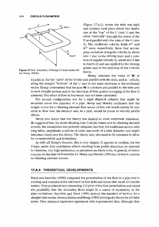
424 CORIOLIS FLOWMETERS
Axis 1
Axis 2
Figure 17.A.1. Geometry of Hemp's U-tube meter (af-ter Hemp 1994b).
(Figure 17.A.1), where the tube was rigidand rotation took place about two shafts:one at the "top" of the U (axis 1) and theother "vertically" through the center of theU and parallel with the sides of the U (axis2). The oscillatory velocity fields v(1) andv(2) were, respectively, those that accom-pany a rotation of angular velocity Qi aboutaxis 1 due to the driving force and a rota-tion of angular velocity Q2 about axis 2 dueto forces of unit size applied to the sensingpoints and in the direction of the Coriolisforces.
Hemp obtained the value of W asfor the "sides" of the U-tube and parallel with the sides, and as — plQiQ2
along the straight "bottom" of the U and in the same direction as the rotationalvector. Hemp commented that because W is constant and parallel to the tube axisin each straight section and in the direction of flow, perfect averaging of the flow isachieved. The effect of flow in the bends had not been calculated.
The second configuration was for a rigid elliptical cylinder that might bemounted across the diameter of a pipe. Hemp and Hendry confirmed that theweight vector for a vibrating element flow sensor of this sort would mainly be sen-sitive to flow near the element and, in a pipe, would be prone to velocity profileeffects.
Hemp also stated that the theory was limited to small amplitude vibrations.He suggested that, for short vibrating tube Coriolis meters and in vibrating elementsensors, the assumption was probably adequate, but that, for traditional meters withlong tubes, amplitudes could be of order one-tenth of a tube diameter and mightintroduce errors into the theory. The theory may also need to be extended to allowfor compressibility and turbulence.
As with all Hemp's theories, this is very elegant. It appears to confirm, for theU-tube meter, that installation effects resulting from profile distortion (as opposedto vibration, very high turbulence, or pulsation) are likely to be, in general, of minorconcern in this type of flowmeter (cf. Hemp and Hendry 1995) but of major concernin vibrating element sensors.
17.A.3 THEORETICAL DEVELOPMENTS
Durst and Raszillier (1990) computed the perturbation of the flow in a pipe that isrotating and considered the relevance of flow field and forces that result to Coriolismeters. They produced very interesting 3-D plots of the flow perturbation and raisedthe possibility that the secondary flows might be a source of asymmetry in thepipe oscillations. Raszillier and Durst (1991) derived the equation of motion for astraight-tube meter, whereas Sultan and Hemp (1989) developed a theory for a U-tubemeter. They obtained impressive agreement with experimental data, although they

17.A.3 THEORETICAL DEVELOPMENTS 425
indicated that there were various limitations of the theory and that further areas ofwork were still needed. Raszillier and Raszillier (1991) used dimensional argumentsto show the possible interdependence of velocity and density. John Hemp (privatecommunication July 1994) commented that the very useful results of this referenceinclude general expressions for time delay and frequency, showing how they dependon various meter parameters such as Young's modulus and length, and estimates ofthe order of effects of fluid density on time delay and natural frequency. Raszillieret al. (1993) suggested that, by influencing the vibration spectrum, the sensitivityof the instrument may be increased. Raszillier et al. (1994) investigated the effect ofa concentrated mass at the middle of the Coriolis pipe segment as required for thepurpose of symmetric excitation of the vibration. The flowmeter factor was foundto be almost independent of the mass up to fairly high values compared with themass of the fluid-filled pipe segment, although the frequency of the fundamentalmode is strongly influenced. Lange et al. (1994) examined the effect of detectormasses on the calibration of Coriolis flowmeters. They showed that the position ofthe detectors must be chosen with care because it may have implications for theaccuracy to which the calibration of the meter remains independent of the fluiddensity. The calibration becomes dependent on fluid density if the detector massesare not negligible compared with the pipe mass. They suggested the most appropriatepositions for the first symmetric and the first antisymmetric vibration modes (cf.Sultan 1992).
Hemp's (1988) reciprocity concept for flowmeters to reduce zero drift errors mayalso be applied to Coriolis meters.
Watt (1991) used a simple Coriolis force model and applied it to obtain thetube distortion for an Endress and Hauser ra-point type tube using a finite elementcomputer analysis. His work confirmed that the highest stresses were around themidpoint where the tube is driven and at each end. He makes the point that theCoriolis distortion of the tube will modify the Coriolis forces compared with a tubein pure bending.
Hemp and Sultan (1989) explained the concept of effective mass of bubbles ina liquid and calculated the expected error. Compared with Grumski and Bajura's(1984) measurements, the theory overestimated the error possibly due to interactionbetween bubbles.
Pawlas and Pankratz (1994) discussed their CFD analysis of flow in Coriolis tubesand outlined their plans for an iterative approach to linking structural analysis of therotation of the flow tube with fluid mechanics analysis to obtain a spatially varyingrate of rotation and hence the pressure distribution on the tube wall, in part due toCoriolis forces.
Hemp (1996) used dimensional analysis (cf. Raszillier and Raszillier 1991) to ex-plore the design requirements if the meter was to be used with low mass flow rates(e.g., when applied to gases near normal temperature and pressure). His findingssuggest that the most appropriate type of sensing transducer in this case is the dis-placement transducer and that the likely requirements, keeping maximum strainunchanged and retaining similarity in layout, will be a reduction in tube diameterto one-third or so and wall thickness to about one-quarter while retaining the samelength of pipe.

426 CORIOLIS FLOWMETERS
Keita (1994) provided a very useful discussion of the various equations used topredict the behavior and the sources of calibration shift in Coriolis meters for gas flowmeasurement. He concluded that the main contribution to the shift in the meterfactor was due to pressure, that the compressibility effects were very small and partlycompensate for the pressure effect, and that, despite the high resonance frequencyof straight-tube flowmeters, they were suitable for gas flow measurement.

CHAPTER IB
Probes for Local Velocity Measurementin Liquids and Gases
18.1 INTRODUCTION
We resort to probes for flow measurement for three main reasons:
i. To provide a low cost method of flow monitoring;ii. To provide an in situ calibration;
iii. To obtain fine detail of the flow in the pipe (velocity profile, swirl, and turbu-lence).
For our present purposes, we shall not consider (iii). It is relevant to fluid mechan-ics research, mainly uses hot-wire and laser doppler anemometers, and is, therefore,outside the scope of this book. We will concentrate on work relating to bulk flowmeasurement. In situ calibration techniques are covered in Chapter 4. In this chap-ter we shall consider the various devices that have been used and are commerciallyavailable either as a local flow monitor or as the probe for in situ calibration. How-ever, before considering these, we need to understand what is being measured.
i. Ideally the probe measures the local velocity and obtains a representative valueof the mean velocity from the shape of the velocity profile. Alternatively, it maymeasure the complete profile.
ii. In practice the probe may be in error because:• it was calibrated in an approximately uniform profile or on the pipe axis but
will need to measure velocity profiles that result in a significant variation ofvelocity across the sensing head;
• it will alter the flow by its presence; and• the flow pattern will continue to change as the probe head is inserted farther
and farther into the pipe and as it approaches the opposite side of the pipe.In some cases, these flows may be analyzed theoretically, but in most cases onewould expect to calibrate the probe, and this calibration will be different at thepipe axis and at the pipe wall.
iii. The probe will reduce the flow area of the duct by its presence, and the area willcontinually decrease as the probe is inserted farther. This blockage will need tobe allowed for. The blockage will also differ between incompressible and com-pressible fluids.
Our object in using a probe is to obtain the best measure of the local flow ratethat can be obtained. We shall need to remember both the limitations of the probe
427

428 PROBES FOR LOCAL VELOCITY MEASUREMENT IN LIQUIDS AND GASES
and the uncertainty of the relationship between the reading and the mean velocity.We also need to remember that, to deduce the mean flow rate in the duct, there isuncertainty in the measurement of the cross-section of the pipe and the blockagecaused by the probe.
The variation on one probe, according to tests by the National Engineering Lab-oratory in Scotland, suggested that blockage at the center for pipe sizes from 250 to750 mm ranged between about ±5% and the change as the probe moves from thecenter to the wall can be of order 10%.
For any new probe design, there is clearly a need for some careful work as to
a. what velocity the probe is measuring in an ideal uniform flow;b. how the signal will change in a real, nonuniform pipe flow, and when close to
the wall; andc. how the flow in the duct will be altered by the probe and how the local probe
measurement would relate to the flow in the duct if no probe were present.
In Section 2.3 and, specifically, in Table 2.2, we noted that the velocity in a turbu-lent flow at about the 0.76 radius point (0.24 of a radius in from the wall) is practicallyequal to the mean flow in the pipe. So this suggests that the probe should be set atthis point. However, this may result in reduced precision due to the shape of theflow profile in this region (b), the level of turbulence, and the proximity of the wall.
18.2 DIFFERENTIAL PRESSURE PROBES - PITOT PROBES
Using Equation (2.10), but introducing a factor k for nonideal conditions, we canobtain the pressure rise when flow comes to rest in the entrance of a pitot tube(Figure 18.1) as
, Stagnationpressure
line
Statictapping
Pitot tube
Figure 18.1. Separate pitot and static tubes.
Ap= \kpV2 (18.1)
For ideal conditions k = 1. Ap is the dif-ference between the stagnation pressure atthe mouth of the pitot tube and the staticpressure; in this case, it was obtained witha wall tapping in the same cross-sectionalplane as the mouth of the pitot tube. Thestatic pressure at the wall tapping will be thesame as the value at the pitot tube assum-ing that there is no cross flow in the tube.The measurement assumes that any pres-sure effects caused by gravity between thepitot tube entry and the wall tapping will beequal for both the total and the static mea-surements and will, therefore, cancel out.
Figure 18.2 shows two forms of pitot-static tube used to obtain the dynamic pres-sure or velocity head. Figure 18.2(a) is a

18.2 DIFFERENTIAL PRESSURE PROBES - PITOT PROBES 429
FLOW 1 or 2 ringsSTATIC o f 7 h o l e s
TAPPINGS
(b) /AFigure 18.2. Two designs of pitot-static tube commended by Bean, both similar to NPL designs(reproduced from Bean 1971 with permission of ASME): (a) Round-nosed pitot-static tube;(b) Conical-nosed pitot-static tube.
diagram of a tube recommended by Bean (1971). A National Physical Laboratory (UK)design appears to differ in that it has an ellipsoidal nose, which is claimed to be lesssensitive to lack of smoothness between the tip and the cylindrical section. Figure18.2(b) shows an alternative design. Note in Figure 18.2 the coaxial arrangement ofthe tubes so that the total pressure is carried in the center of the tube and the staticpressure is carried in the outer annulus. Note also the sensing holes for the staticpressure. Bean (1971) recommends that d should be between about 5 and 8 mm(re to & in.)-
At low Reynolds number based on the tube diameter (<100) when the effect ofviscosity becomes important, k diverges from unity. Goldstein (1965) gave k valuesfor conical entry and round-nosed designs in the range 1.020-1.055 at about 0.6 m/s(Re « 300), a minimum value of k = 0.991 at about 3-3.5 m/s (Re 1,600-1,900), anda value within about 0.1% of unity for 6-27 m/s (Re 3,000-10,000). Bean (1971)also reckoned that, for correct alignment (less than 12°), the reading should bewithin 0.3%. For further information, the reader is referred to ISO 3966 or Owerand Pankhurst (1966).
At high velocities in a gas, there are compressibility effects. The simple Equation(18.1) has to be replaced by one that allows for these effects. Using Equation (2.16)
(2.16)
where M2 = pV2/(yp) for a perfect gas, we obtain a modified equation for V
V =\
2y p\(Po\y-1)/y
-\p \\p) (18.2)
Bean (1971) suggested that, below about 15 m/s for air at sea level, there isnegligible difference between this value and that from Equation (18.1) (with k = 1).

4 3 0 PROBES FOR LOCAL VELOCITY MEASUREMENT IN LIQUIDS AND GASES
We can see this if we rewrite Equation (18.2) as
+ p)
If we then use the binomial theorem to expand the inner bracket, we obtain
V2 =2y p f | y - \ Ap
y - 1 p \ y p(18.4)
assuming that we can neglect terms of order (Ap/p)2 and greater. This reduces to
V2 =2Ap (18.5)
In neglecting terms of order (Ap/p)2 or greater powers, we have neglected terms oforder (\pV2/p)2 or greater. If p = 1.3, V = 15 m/s, and p = 105 Pa (1 bar), then theerror resulting from ignoring \pV2/p is of order 0.15%, confirming Bean's value.
One major problem with the pi tot tubeis the effect of unsteady flow on its read-ing, and because turbulence is very com-mon in normal industrial flows, the pitottube will tend to read high (cf. Goldstein1936). MacMillan (1954) discussed the ef-fects of low Reynolds number and noted(MacMillan 1957) that in a shear flow therewas an apparent shift in the effective centerof the pitot tube of 0.1 Sd in the direction ofhigh velocity, where d is the outside diam-eter of the pitot tube.
One manufacturer offers a device thatis not strictly a pitot tube (Figure 18.3) butconsists of a cylindrical probe with sensingat the end. The differential pressure result-ing from the flow acts on a spring-loaded di-aphragm, the movement of which is sensedby an inductive displacement transducer.Bean (1971) refers to designs with upstreamand downstream pointing tubes, (cf. Cutler1982)
Figure 18.3. Probe-type differential pressure sensor[reproduced with permission of Laaser (UK) Ltd.].
18.3 DIFFERENTIALPRESSUREPROBES-PITOT-VENTURI PROBES
In order to increase the pressure differencein the pitot tube in low flow rates, thepitot-venturi has been used. In this device,the total pressure is compared with a de-pressed pressure created by the flow at the

18.5 INSERTION TURBINE METER 431
(a)
throat of the venturi. This is shown inFigure 18.4(a) (Bean 1971). The pressure dif-ference can be increased even further by us-ing a double venturi [Figure 18.4(b)]. Theouter venturi causes a reduced pressure atthe outlet of the inner venturi, thus increas-ing the flow through the inner one and re-ducing the throat pressure even more.
Another device depending on differen-tial pressure and having some similaritiesto a venturi is the Elliot-Nathan flow tubeillustrated by Hayward (1977c), which ap-pears to have a sharply converging and di-verging venturi, in the diverging portionof which is a hollow cone in which thedownstream pressure is measured. Haywardcommented that it is claimed to have anoutstanding performance. However, strictlythis is a full-bore meter, since its installationwould have to be in a spool piece.
Cairney (1991) described the use of abidirectional pitot-venturi inserted into thebled-steam line of a generating plant inwhich there was a possibility of a flow re-versal due to a major transient in the sys-tem. The device consisted of two very small venturi meters with axes parallel butfacing opposite directions in which the differential pressure was measured betweenthe throats. The device was sensitive to Reynolds number and turbulence level.
Figure 18.4. Pitot-Venturis (Bean 1971; reproducedwith permission of ASME): (a) Single venturi; (b)Double venturi.
18.4 INSERTION TARGET METER
The flow acts on the disk (Figure 18.5), which is supported by a lever. The smallmovement of the lever is sensed by an inductive displacement, counterweight, ormagnetic coupling to a pneumatic sensor. Liquid flows can be measured in a rangeof about 0.05-4 m/s and gas flows from about 0.6 m/s up to about 5 m/s. It may beapplicable to temperatures up to 500°C. Measurement uncertainty for gas flows isclaimed as ±1.5% measured value.
18.5 INSERTION TURBINE METER
18 .5 .1 GENERAL DESCRIPTION OF INDUSTRIAL DESIGN
The insertion turbine flowmeter is a small diameter turbine and pickup on the endof a relatively small diameter probe, usually inserted into the pipe via an isolationvalve. The propeller may be able to cope with velocities for liquids of 0.1-12 m/s orpossibly higher, and for gases of 1 m/s or less to 50 m/s or possibly more, with a range

432 PROBES FOR LOCAL VELOCITY MEASUREMENT IN LIQUIDS AND GASES
Figure 18.5. Insertion target disk flow probe [repro-duced with permission of Laaser (UK) Ltd.].
for one probe of about 10:1. An operatingrange of as much as 100:1 may be quoted insome designs. The turbine probe, shown inFigure 18.6 retracted into the threaded pipefitting, may have ball bearings, jeweledpivot, tungsten carbide journal, or other.Ideally this will result in a rotational speedfor a limited range proportional to the flowrate past the head. There is likely to be aminimum velocity for which the propellerwill turn and another for which it can beexpected to give results within the normalprecision. For very low drag, the pickupmay be radiofrequency or other low dragtype. A typical manufacturer's specificationfollows:
15-30 mm
±0.5-1% of full scale0.05-0.25%10:1Stainless steel-200 to 150°C
Diameter ofrotor
LinearityRepeatabilityTurndownConstructionTemperature
rangeThe turbine is inserted through an isolationvalve of through-bore type with a clearconcentric opening of diameter dependingon the meter. The complete device consists,typically, of a small stainless steel turbineon the end of the stainless steel insertiontube (Figure 18.6). External handles mayindicate the alignment of the probe, andthis should be axial to avoid errors.
insertion StemDepth indicatorSeal ClampSeal HousingTurbine Rotor Cage
& AssemblyPressure Transducer
Tapping
Figure 18.6. Insertion turbine probe showing the turbine cage retracted into the screwed pipefitting (reproduced with permission from Flow Automation (UK) Ltd.). Note: Figure is drawnfor clarity, not correct alignment.

18.5 INSERTION TURBINE METER 433
The insertion tube passes through an outer tube, which seals the line pressure.When this pressure tube is inserted into the valve, the valve can be opened, and theturbine can be inserted through the valve into the line. Fluid seal mechanisms needto avoid leakage but allow the probe to be inserted. In high pressure applications,inappropriate selection can result in the probe's being expelled from the process line,or at least moved from its set position.
These probes are suitable for water and hydrocarbons, particularly the latter be-cause of their lubricating properties. They are not likely to be suitable for high ve-locities or hot water.
If such a probe is to be inserted and used as a single reading device for pipe flowmonitoring, then the position of the probe in the pipe will need to be carefullyconsidered as discussed earlier.
To obtain a full flow profile, a series of measurements can be made, and the resultscan be integrated to obtain the flow rate. There is usually a limit to the proximity tothe pipe wall at which measurements can be made. However, the nonslip conditionat the wall should allow a curve to be fitted for this region. The profile shape thusdetermined allows the computation of volumetric flow. In this mode, they are alsoused for in situ calibration, although the overall uncertainty is likely to be in therange ±2-5%.
Various other designs of wall-mounted probe are available for hot-tapping orfitting into a T-piece in the wall. An example is shown in Figure 18.7. These paddle-wheel-type probes essentially measure flow near the wall of the pipe, and the deduc-tion of mean flow in the pipe will be obtained by reference to the manufacturer'sliterature.
18.5.2 FLOW-INDUCED OSCILLATIONAND PULSATING FLOW
Small diameter probes at the center ofa pipeline of, say, 2 m diameter or greater,with high velocity flow, are prone to oscil-late. This may appear as a pulsation but canlead to failure of the support tube in ex-treme cases.
Ower (1937) developed a theory for avane anemometer, showed that it overesti-mated average air speed, and obtained anexpression for the error. Experiments con-firmed the theoretical conclusions.
Jepson (1967) investigated the effectof pulsating flow on current meters andconcluded that fluctuations of the veloc-ity vector parallel to the mean flow al-ways cause overestimation, whereas fluctu-ations perpendicular generally cause under-registration. He suggested that errors couldbe reduced by
Figure 18.7. Paddle-wheel-type flow sensor (repro-duced with permission of Peek Measurement).

4 3 4 PROBES FOR LOCAL VELOCITY MEASUREMENT IN LIQUIDS AND GASES
a. using blades with a large aspect ratio,b. making the tip-to-tip diameter small to keep the blade thickness as small as
possible,c. keeping the blade angle to a minimum, andd. using low density material for the rotor.
Jepson's paper is a useful source of earlier references on current meters.
18.5.3 APPLICATIONSApplication of turbine probes to large diameter pipe flow measurement should beundertaken with care, recognizing the need for an integration routine, the blockageeffect caused by the probe, the effect of wall on probe calibration, the errors inmeasurement of pipe diameter, and the total uncertainty of final value of flow rate.
Turbine probes have been used in applications such as compressor efficiency andsurge control, pipeline leak detection, odorizers, samplers, and checking through-put. Some have claimed that this device can be used for custody transfer to mea-sure with high accuracy and reduce cost by avoiding the purchase, installation, and
15 ins (381mm)
Junction Box
Alignment handle
- Positive stem lock
Seal housing
Isolation chamber
Figure 18.8. Mauflo crude oil insertion flowmeter (reproduced with permissionfrom F.M.A. Ltd.).

18.7 INSERTION ELECTROMAGNETIC PROBES 435
maintenance of a large bore flowmeter. In my opinion this is rarely likely to beachievable. However, if calibrated in situ, the probe may provide a long term checkon performance, although short term repeatability may not be so good.
Another device has been developed for crude oil flow measurement (Figure 18.8)and consists of a rotor of up to 140 mm diameter that is capable of coping with waxand fibrous materials in the flow. For a flow range of 0.15-12 m/s, the uncertaintyis claimed to be about ±0.3% at the top of the range and ±5% at the bottom with arepeatability of ±0.15%.
Raustein and Fosse (1991) used insertion turbine meters for fuel gas flow mea-surements and estimated measurement uncertainty as ±2-5%. They are also usedfor flare gas metering where it appears that uncertainty is likely to be in the range±5-10%.
18.6 INSERTION VORTEX PROBES
A commercial vortex-shedding insertion probe, which has been available in the past,had a rectangular slot in the end of the insertion bar (about 32 mm diameter), andthe bluff body spanned this perpendicular to the axis of the bar. The insertion barwas retractable and of length up to about 900 mm. A turndown of 20:1 was claimedwith repeatability of 1-1.5% of reading.
18.7 INSERTION ELECTROMAGNETIC PROBES
Insertion electromagnetic probes have been the subject of considerable develop-ment, and their performance has been analyzed by Hemp (1995b) and Zhang andHemp (1994, 1995) to obtain the sensitivity of its signal to proximity to the wall.Industrially, it has also advanced in terms of accuracy and of low power usage.
The probe shown in Figure 18.9(a) is claimed by the manufacturer to have arange up to about 5 m/s, the actual maximum depending on the insertion lengthwith maximum flow allowed for insertions of 300 mm or less. The accuracy is givenas ±2% of rate or ±2 mm/s, whichever is the greater. Insertion is up to 1 m withtypical materials for wetted parts of stainless steel and PVC. The temperature rangefor water is given as 0-60°C. It is designed for local measurement of water velocity.Figure 18.9(b) shows the installation arrangement (cf. Baird 1993 who described aninsertion probe for pipes of 25-300 mm).
These devices in various forms have been tried out for current flow measurement,for ships' logs, and for pipe flows for many years. For more references, the reader isreferred to an earlier review by Baker (1983).
One manufacturer offers probes with different sizes of discus-shaped head, inone case with a spherical head with electrodes projecting radially, and in anotherwith a ring with electrodes projecting radially inward. The heads are directionallysensitive and operate at 128 Hz. The measurement uncertainty is claimed as 1% ofreading + 5 mm/s, and the direction is claimed to be better than 5° (cf. Bowden andFairbairn 1956).
Another insertion probe, but for axial insertion, was developed for blood flow inarteries (Mills 1966, cf. Baker 1968).

436 PROBES FOR LOCAL VELOCITY MEASUREMENT IN LIQUIDS AND GASES
(b)
Figure 18.9. Electromagnetic-type insertion probe (reproduced with permission from ABB Ltd.):(a) Pipe insertion probe; (b) Insertion arrangement.
18.8 INSERTION ULTRASONIC PROBES
The doppler ultrasonic principle lends itself to applications as a flow probe, providedthere are sufficient scatterers in the flow; most of the reservations have already beenset out in Chapter 13.
A very much more precise instrument, depending on the transit-time principle,has been developed by Rawes and Sanderson (1997). The device consists of a bar,with ultrasonic transducers on each end, that is inserted through a fitting in the pipewall. Once in, the bar is turned into the flow so that it lies parallel with the pipe axis.It is then possible to send ultrasonic pulses from one transducer via reflections onthe pipe wall to the other, both up- and downstream. This may lead to quite wideflow coverage and flow averaging. Its performance, even downstream of disturbingfittings, appears to be better than ±2.5% for higher flow rates. Figure 18.10 showsthe essentials of this meter.
Olsen (1991) reported on the use of transit-time techniques to measure air veloc-ity. The frequencies used were 3.1 Hz (sonic) and 40 kHz (ultrasonic). He claimed thatthe precision was better than a pitot-static tube and that the small size, simplicity,and low price compared well with other methods.

18.10 CHAPTER CONCLUSIONS 437
PIPE
REFLECTOR
Figure 18.10. Ultrasonic-type insertion probe (after Rawes and Sanderson 1997).
18.9 THERMAL PROBES
Thermal probes are used so frequently as part of a full-bore flowmeter spool piecethat they have been included in Chapter 15.
18.10 CHAPTER CONCLUSIONS
The turbine insertion probe has been an essential workhorse of the industry andis likely to continue to be, particularly where nonconducting liquids and gases areinvolved.
The latest developments in electromagnetic probes are very promising, and fur-ther designs and developments may well appear.
The novel ultrasonic meter of Rawes and Sanderson (1997) may well set a newstandard for precision in the measurement of bulk flows using insertion methods. Itis likely to be the subject of considerable development, in order to perfect both themechanical insertion system and the ultrasonic sensing and averaging procedure.
No doubt a further area of development will be the secondary equipment and itsability to obtain the best averaging of flow traverse data or of the ultrasonic response.
One of the weakest parts of in situ calibration using insertion probes tends tobe the measurement of internal pipe dimensions. The ultrasonic techniques shouldprovide a precise means of achieving the cross-sectional area.
The problems of blockage and the effect of wall proximity on the flow aroundthe probe may lend themselves to computational modeling. However, the ultrasonictechniques may, again, offer a means to obtain the profile modifications due to theprobe.

CHAPTER 13
Modern Control Systems
19.1 INTRODUCTION
This chapter does not attempt more than a cursory review of modern control sys-tems, as it is outside my main area of expertise. Those knowledgeable in electronicsand control will pass quickly over this chapter! Others who wish to delve moredeeply may, for instance, turn to Sanderson (1988), Brignell and White (1994),or other experts, or for a good, recent introduction to the control of machineryFoster (1998) is recommended. I am pleased to acknowledge valuable insights ob-tained from Cranfield lectures given by Bill Black, David Clitherow, Doug de Sa, andothers.
This book is about flowmeters that depend, in the main, on mechanical orthermo/fluid mechanical effects. In only one case of mainstream meters, the elec-tromagnetic meter is the signal electrical throughout. The aim of the book has beento bring together information on the performance of these meters based on physi-cal, experimental, and industrial experience. I have made the assumption that theelectrical signal interpretation, which is based in the meter, is capable of doing thejob set by the designer of interpreting the meter output into a standard electricalform. This assumption is not always adequate (e.g., where electrical signals from thesame instrument do not appear to agree with each other). Nevertheless, the devel-opments in design of electrical systems are assumed to be such that the reader willnot benefit from a detailed description or that the circuit will be changing so fastthat any statement will be out of date.
Once the signal is available, we shall need to feed it into the overall control sys-tem. It is clear that if it does not match the rest of the control system's protocol,conditioning may be necessary, but this is an expert job, and detailed signal condi-tioning will not be undertaken lightly. In many cases, interface modules that do thisconversion will be available.
From the time when process operators adjusted valves to control flows on thebasis of visual flow readings, electrical control has steadily replaced the operators'functions. Like the operators, the sensitivity of the electrical systems could resultin undercorrecting or overcorrecting and could cause unstable operation by ampli-fying the natural fluctuation of the process. The operator then needed to keep aneye on the automatic control and intervene if necessary. These control systems wereanalogue. They used an electrical signal and amplified it, integrated it, and differ-entiated it in a way analogous to mathematical actions. However, the operator wasalways ultimately responsible for setting the values and able to override if necessary.
438

19.1 INTRODUCTION 439
The advent of digital computers allowed the acquisition of much more data andmore detailed assessment of the performance of the plant.
However, as digital computers superseded (largely) analogue computers, so digitalcontrol has superseded analogue control in many cases so that the computer canrespond to signals and adjust the plant in a far more detailed and sophisticated way.
19.1.1 ANALOGUE VERSUS DIGITALSignal conditioning is a major subject in its own right, and the reader is referred toother sources such as Sanderson (1988). Sanderson classifies transducers by
• type of output - voltage, current, or charge;• type of signal - unidirectional, bidirectional, alternating, or transient;• information content of signal - by level or by amplitude, frequency, or phase
modulation of a carrier wave;• relationship between physical variable and electrical output - linear or nonlinear;
and• output impedance.
Analogue signal conditioning is often to
• convert output to voltage;• change impedance as required; and• amplify, filter, demodulate, and linearize.
From classical control theory with its sophisticated mathematics and relativeinflexibility, the modern control systems use the power of the computer to overseethe process, to question the sensors, to identify problems and rectify them, and toprovide the operator with a vast amount of information and control, but they arepackaged in a way that is easily accessible.
Distributed control systems (DCS), which are analogue, need to be fast withhigher bandwidth and built-in redundancy (e.g., for the petrochemical industry).
In much primarily mechanical plant, the control was originally exercised byelectromechanical relays. These relays would control the electrical power to thecontrolling elements in the system (e.g., valves). When these were superseded byprogrammable logic controllers (PLC), the logic used in the relays was carried overas ladder logic.
One most important feature of digital systems is that they are less susceptible tointerference in that they can carry their own checking protocol within the message.
19.1.2 PRESENT AND FUTURE INNOVATIONSA major step in the move toward modern control was to remove the analogue sys-tems that were much less flexible, and could not easily be reprogrammed by a com-puter command, and to introduce the microprocessor. This then allowed a furthersophistication - the individual instruments became intelligent and were able to beinstructed to do simple tasks and, in turn, could provide much more informationto the central computer. The computer could store past information and comparepast performance with current operation, thus providing further checks on plantperformance and safety.

440 MODERN CONTROL SYSTEMS
This led to the idea that the communication system could be a signal highway(or bus), to which any instrument with the right protocol and any computer couldbe connected. The signal highway could be of copper, but equally could be of opticalfiber, electromagnetic waves, or superimposed signals carried by the electricity mainor telephone lines. Transmitters and repeaters could then include satellites, and thesystem could be, essentially, unbounded.
At the other end of this communication link is the computer or computers thatcontrol the process and that will be able to work in tandem if necessary, and the plantoperators will work to visual display unit (VDU) screens with the latest windowspresentations and graphical portrayal of each part and aspect of the plant and itsoperation.
All this requires a generally accepted common communication language or pro-tocol to which instruments and systems conform and that will ensure each messageis correctly sent and received, without interference.
Modern telemetry systems provide the means of controlling plant and measuringits performance from a central station. The three aspects of the process are
• the measurement technology, which has been the prime subject of this book. Themicrocomputer has revolutionized this technology with smart and intelligentinstrumentation. One aspect that may need attention is signal conditioning.The signal from a sensor may not be suitable for a system and may need to beadapted: from analogue to digital, from digital to analogue, or other change.
• the method of transmission, which, having been by means of copper wires formuch of its history to the present, is now the subject of continual and highlysophisticated alternative developments.
• the controls, both instrument outputs and process adjustment means. From di-rect, but remote, control of instruments, through analogue computers, this hasnow firmly arrived at digital computer techniques.
19.1.3 INDUSTRIAL IMPLICATIONSThe range of industries is now very wide and includes water and sewage treatmentand distribution, oil and gas production and pipelines, process industries of all sorts,and manufacturing including the production of flowmeters. The techniques are, ofcourse, not limited to process flow but can also be used in the electricity genera-tion and distribution industry, the electrical power transmission industries (e.g., railnetworks), building services, and lighting control.
This means that the typical company supplying such equipment and systemsis increasingly a software-based company, using proprietary equipment and supply-ing the software for the control station and the outstations, and using whichevertransmission system is most appropriate to the task and the customer's needs.
19.1.4 CHAPTER OUTLINEThis chapter provides an overview of how the signals from these meters are used inthe control of plant. In referring to meter or flowmeter, the reader should understandthat broadly the same will be true of other instruments within the system. I shallstart from the assumption that, despite increasing coordination between signal spec-ifications (protocols), there is still sufficient variation to make it impossible to use

19.2 INSTRUMENT 441
an unconditioned signal from any instru-ment. The modern control systems will,therefore, in some form, require the follow-ing components (Figure 19.1):
a. the instrument;b. an interface box that translates electri-
cal signal to and from the instrumentinto a signal as required by the remain-der of the system;
c. a communication language or protocol;d. a communication medium;e. an interface that receives the signals
and translates them to the computerprotocol;
f. a computer that receives signals,checks their validity and appropriate-ness against limits, models, and pastexperience; transmits control informa-tion to both meters and valves, etc.;and displays its actions with the maxi-mum user accessibility.
COMPUTER SYSTEMS
INTERFACEBOXES
BUS
INTERFACE BOXES
COMMONPROTOCOL
INSTRUMENTS ON THEPROCESS PLANT
FLOWMETER
Figure 19.1. Main components required for a moderncontrol system.
19.2 INSTRUMENT
19 .2 .1 TYPES OF SIGNAL
The rest of this book is about the details of the flow sensor and how it senses a flowof fluid and converts this into an electrical signal. The signal will usually be one ormore of the following:
• an analogue signal of 0-20 or 4-20 mA or a voltage or a resistance;• a frequency signal - this may be of high or low frequency or both;• a digital signal in which the flow quantity is transmitted in a numerical form,
more likely to be binary than decimal;• an intelligent communication that allows the sensor to provide more than one
piece of information, and the user, through a computer, to instruct the sensor(and other devices) in various ways.
Twenty-five years ago we were concerned with the cleanness of the signal, whichcame from a meter and provided just one parameter, the flow. The advent of com-puting power, and particularly the microprocessor, has allowed more informationfrom the signal to be interrogated and multiple outputs to be handled. Thus interestis now being shown in the details of the noise in the signal, which previously wesmoothed out and discarded.

442 MODERN CONTROL SYSTEMS
19.2.2 SIGNAL CONTENTAmadi-Echendu and Hurren (1990) (cf. Amadi-Echendu and Higham 1990, Amadi-Echendu and Zhu 1992) discussed the use of noise in flowmeter signals to obtaininformation about the condition of process plant and condition monitoring in gen-eral. For instance, the variation of pulse spacing in a turbine meter may be obtained,and the nature of this fluctuation may be interpreted as due to the signature ofthe plant made up of pulsatile flow, etc. Change in the signature may indicate achange in conditions in the plant. To date, there does not seem to be much theoreti-cal analysis to help our understanding of the relationship between secondary signaland the physical fluid behavior. However, some recent work by Krafft et al. (1996)has started to do just this by developing the theoretical prediction of the effect ofair bubbles in a magnetic flowmeter and comparing this to the signal obtained.
The microprocessor has allowed a further, and major, step. It is now possible tobuild into the instrument means for checking the validity of the signal, for adjustingrange, and for selecting the form of signal. The meter may, therefore, be capable bothof transmitting and receiving information.
For such meters, the terms smart instrument and intelligent instrument werecoined and associated with various degrees of on-board computational power. Thedefinition of these terms can be found in Higham and Johnston (1992), but the con-tinual developments resulting from microprocessor power mean that the distinctionis likely to become less relevant or used. They suggested that smart be applied to sen-sors that automatically compensate for nonlinearity, temperature effects, etc., andcan be configured before installation to provide a predetermined range and span.However, they would normally need to be taken out of service to be reconfigured.
The term intelligent includes the smart features, but also implies two-way com-munication with the control system either by a separate communication port or bya superimposed digital signal on the 4- to 20-mA signal. This greatly increases theversatility of the sensor, allowing self-diagnostics and other routines and commandsto be sent from the control system to the instrument.
Brignell and White (1994) list the principal subsystems within an intelligentsensor as
• a primary sensing element,• excitation control,• amplification and possibly variable gain,• analogue filtering,• data conversion,• compensation,• digital information processing, and• digital communications processing.
A most important attribute of the intelligent sensor is addressability, which is anecessary part of the bus communication, but it also will put time constraints onthe signal transmission each way. Thus the instrument's microprocessor
• processes signals from one or more sensors and replaces complex analogueelectronics;

19.3 INTERFACE BOX BETWEEN THE INSTRUMENT AND THE SYSTEM 443
• is capable of re-ranging, diagnosing problems, etc.;• oversees the communication of the sensor with the wider control system; and• manages display functions if present.
The microprocessor then allows enhanced accuracy by putting in the calibrationcurve, which provides
• high turndown ratios leading to increased rangeability - but beware of hiddenerrors,
• increased manufacturing flexibility, and• increased reliability and with a quicker identification of any problems, an im-
proved maintenance philosophy.
There may be some disadvantages such as a change in working practices, thepossibility of changing ranges without considering safety implications, and the sit-uation of being harder to repair by in-house people and so more likely to lead toa throw away/replacement philosophy. However, many of these problems have thesolution implicit in the new technology, by using passwords, more sophisticatedalgorithms, etc.
19.3 INTERFACE BOX BETWEEN THE INSTRUMENTAND THE SYSTEM
The system designer and builder is unlikely to be the manufacturer of all the instru-ments in the system. There was a trend this way about 25 years ago, but the greaterflexibility of the microprocessor has encouraged control system design to be capableof coping with a variety of instruments from different manufacturers and for variousindustries. Thus, although some instruments may incorporate the interface in thesensor, the simplest arrangement is to have an interface box that ensures a commonsignal protocol. This reflects the comparative cheapness of the microprocessor-basedbox, in comparison with the cost of expert time to adapt an instrument to a partic-ular protocol. These devices are sometimes called controllers and may be capable ofhandling from 1 to 30 or so sensors with individual loops.
The output of this box (to the highway/bus) will be one of the emerging signalprotocols. This will probably be a digital signal that has a code to describe the natureof the particular data set that follows the code. The codes will then define particularinstruments (or control devices) to which the signals are directed or from whichthey come and, in addition, will define the nature of the data, whether flow rateetc., or range, or some other quality. Assuming that these code and data strings willbe vying for space on the same pair of wires, or the same optical fiber, the instrumentwill need to set up a "handshake" arrangement with the rest of the system to allowtime for the signal to be transmitted. This in turn will have repercussions for datatransmission rates.
This type of outstation may also provide local control and may have main andstandby units.
444 MODERN CONTROL SYSTEMS
19.4 COMMUNICATION PROTOCOL
19.4 .1 BUS CONFIGURATION
In the past, connection of sensors to the central control has been in the form ofa star where each instrument communicates via a, usually, wire pair to the center(Brignell and White 1994). There is clearly much cabling required, and it becomesmost dense at the center. The modern alternative, the bus, allows all devices to sharea common pair of wires. Disadvantages are that
• devices need to be addressable and so to have a level of intelligence,• breakage in the bus can cause a loss of communication, and• pressure on the bus may limit time availability for signal transmission.
To overcome the particular danger of bus breakage, a complete loop bus can beused, or even two bus loops separated physically to avoid the common destructionof both.
The system components will use one of the standard protocols, for instance:
• 4 to 20 mA signal for analogue instruments;• digital instruments with digital communication;• flow computer output with serial interface that provides an encoded binary trans-
mission; and• a modern bus with high level, computationally controlled protocols (e.g., HART,
Profibus, and Fieldbus), which interface to intelligent instruments.
It should be remembered that digital information in computers is carried as aseries of Is or 0s and so, for instance, the logic 1 could be portrayed as a burstof higher frequency, whereas the logic 0 would be portrayed as a burst of lowerfrequency. The message would consist of a series of Is and 0s, with indications ofstart and finish of words, and any instrument attached to the cables would respondwhen its call sign was sensed on the bus/highway.
Brignell and White (1994) discussed the ISO's (see ISO 7498-1:1995) seven-layered communications protocol for an Open Systems Interconnect (OSI) strategy.
Physical layer Relates to connections such as physicalconnectors, and electrical procedures forhandshaking, etc.
Data link layer Ensures reliable and error-freetransmission.
Network layer Appears to ensure standard signals andappropriate communication paths regardlessof where the signal originates.
Transport layer Provides a reliable data transfer exchangeservice between the instruments, etc., andthe user.
Session layer Manages the interaction between differentapplications on different systemsconnected to the network.

19.4 COMMUNICATION PROTOCOL 445
Presentation layer Ensures a common data format.Applications layer Provides services that can be accessed
and used by the computer systems.
These cover, broadly, the levels (a) to (f) in Section 19.1.4.
19.4 .2 BUS PROTOCOLS
Manufacturing Applications Protocol (MAP) is based on the seven-layer ISO/OSImodel. General Motors was largely responsible for its development (Brignell andWhite 1994). Statistical tasks for optimizing production, order processing, planning,and different logistical services may be available from such protocols (Lindner 1990).However, MAP is not widely used as a general-purpose instrumentation standard dueto the severe requirements for the hardware/software processing resulting from thefull seven-layer protocol.
Wood (1994) described HART and Profibus as examples of proven specificationsthat provided background and influence for the modern fieldbus proposals.
Highway Addressable Remote Transducer (HART) digital communications pro-tocol developed by Rosemount (Brignell and White 1994) uses digital techniques toallow an intelligent instrument to adjust range and span, to undertake flow calcu-lations, to apply self diagnostics, and to communicate (Howarth 1994). HART usespoint-to-point or all-digital modes. In the former, it superimposes digital data on a4 to 20 mA signal by two defined frequencies of ±0.5 mA amplitude: 1,200 Hz forbinary 1 and 2,200 for binary 0. Message rates are typically three per second. It usesa master/slave protocol (Brignell and White 1994) in which the master is the onlydevice that may initiate a message transaction. Up to two masters can communicatewith connected field instruments, typically a hand-held communicator and a con-trol system or PC-based workstation. At the applications layer, HART commands areof three types: universal commands to read an identifier, variable, or current; com-mon practice commands (e.g. calibrate or perform self test); and transmitter-specificcommands (e.g., start/stop totalizer, read density calibration factor).
Profibus was set up by a group including AEG, ASEA Brown Boveri, Honeywell,Klochner-Moeller, Lands & Gyr, Robert Bosch and Siemens, with the objective ofcreating a digital fieldbus standard consistent with the ISO/OSI model in ISO 7498(Squirrell 1994).
Interoperable Systems Project (ISP) was formed in 1992 (Allen 1994) with theobjective of achieving a single, open, interoperable, international fieldbus.
World FIP (Desjardins 1994) was to promote the acceleration of a viable interna-tional fieldbus standard of manufacturing and process control and resulted from amemorandum of intent in 1993.
The ISP and World FIP (North America) combined in 1996 to form FieldbusFoundation, which produced in 1998 an interoperable replacement for 4 to 20 mAcontrol, that is at least as reliable and replaceable. Members represent instrumentsuppliers and end users.
Fieldbus is a communication system specially designed for networking of trans-ducers (Brignell and White 1994). The protocol model has physical layer, data linklayer, applications layer, and also a user layer.

446 MODERN CONTROL SYSTEMS
In conclusion it should be noted that this brief introduction to fieldbuses wasbelieved to be correct at the time of writing, but it should also be remembered thatthere are other fieldbuses available in addition to those mentioned in this section,and the reader should obtain expert advice on the one most appropriate to a partic-ular application.
19.5 COMMUNICATION MEDIUM
19.5.1 EXISTING METHODS OF TRANSMISSIONPneumatic transmission has been used widely in the past and had the great virtueof being intrinsically safe. As with analogue electrical signals, standard signal rangesensure that instruments are compatible and that pressure supply failure will not pro-duce an undetected error. Thus 20-100 kPa and 20-180 kPa are two such (Sanderson1988). It is likely that with optical transmission offering an alternative and, in mostcases, intrinsically safe communication system, and with the inherent compatibil-ity of optical with digital electrical systems, pneumatic systems will become lesscommon.
Analogue electrical transmission depends on a small current, voltage or resistanceto provide the signal from a sensor. Much instrumentation still in service uses thesesignals, and so analogue communication is likely to be around for some time. Againit is likely to decrease, and, indeed, sensors that exploit digital and other moderntechnologies are likely to be designed. Many analogue sensors included a frequencyoutput, which allowed pulses to be counted at the end of the communication lineand a total flow or other parameter to be obtained.
It is now possible to send complete information on parameter values by digitalsignals, which do not need to be converted from a milliampere value to a flow ratebut which provide the flow rate in the required units. In addition, the sensor canbe addressed and will respond to questions or commands. The communication hasthus become two-way.
19.5.2 PRESENT AND FUTURE TRENDSThe means by which the components in a modern control system are connectedare now many and various and exhibit some of the ingenuity that stems from thegreat power of modern signal processing. Thus communication for a conventionalplant may well be via copper wires or, where there are dangers due to explosiveenvironments, via optical cables. The transmission system may be by the publicswitch telephone network (PSTN). A frequency signal is essentially the signal usedin telephone communications and, therefore, in most of the world's communicationby all forms of transmission and in repeater stations such as satellites. For oil andgas, transmission may be by microwave, which requires line of sight between thecontrol station and outstation, or by radio waves bounced off the troposphere orlinked by satellite. A utility may develop means for sending the signals down thepower lines that link every house, whereas an international oil or gas company maybe able to afford radio links via their own satellite or rented satellite space.

19.5 COMMUNICATION MEDIUM 447
Combinations of these and other methods will be selected depending on themost appropriate route for the particular application. For added security, dual meth-ods may be used providing a fall-back in case one method fails. The options are likelyto increase.
The bus/highway will increasingly link computers with control and communica-tion capability and smaller modems with hand-held devices for field checking. Thedevelopment of such data highways is likely, eventually, to lead to the eliminationof all but digital information. Standardization will address the frequency levels ofthe bus, which will affect the speed of response of the instruments.
The sensor will, therefore, be capable of linking with computer control systemsanywhere in the world or beyond and the wire connections may become an antenna.Even the problems of power supply are overcome with local power generation fromsolar, wind, or nuclear sources.
19.5.3 OPTIONSImrie (1994) commented that the type of measurement being made will determineto a large extent the type of communications required:
• Is the variable to be used in a control or a time-critical application?• What is the likely rate of change of the variable?• Is continuous trend monitoring required, or is it event-driven?• Does the sensor lend itself to power saving?
The location will determine security, protection, safety, interference, availabilityof services (e.g., power and signal networks), and the access requirements of owner-ship of land.
The consequence of data loss, the rate of data transfer, the response time, one-way or two-way transfer, and the size of data package all will affect choice.
The nature of the application will be important: control or monitoring, regula-tory and insurance, safety, effect on product or services.
Imrie then went over the options: cable direct connected, service radio, satellitecommunications, mains borne, meteor burst, licensed radio, and delicensed lowpower radio. In addition, careful consideration of networks and protocols and ofpower management is necessary. Imrie suggested the following applications:
For UseReal-time measurement Cable or radio
and/or controlTime critical Cable or radioEvent-driven with a Cable or radio with
fast response appropriate protocolEvent-driven with a A link establishment
slow response network over telephone orservice radio networks, orlow use power radio

448 MODERN CONTROL SYSTEMS
Long-term trend measurement Link establishment networkover telephone or serviceradio networks with overnighthistorical file transfer
Multinode system Suitable network, not multiplepoint-to-point links
19.6 INTERFACE BETWEEN COMMUNICATION MEDIUMAND THE COMPUTER
For a particular company designing a control system, this interface will be essentiallya modem that converts the electrical signal transmitted to the size and form neededby the computer. The transmitted signal will be specified by the protocol or by thecommunication network management, and the other side of the interface shouldbe under the control of the system designer and meet the requirements of thecomputer interface.
19.7 THE COMPUTER
By comparing the operation of the process with models programmed into the com-puter, the system could set the control points, removing operator error and reducingoperator time.
There is wide use of modeling and simulation techniques for areas as diverse asnetwork analysis for water distribution systems, chemical mixing, and pump controlusing software suites (Fowles 1994).
The control station, which will represent the latest in user-friendly presentation,will probably include a computer model of the network, based on predictions suchas those of Miller (1990). Thus, the computer will enable the user to identify on amap where the control is taking place, will provide the user with a virtual controlpanel, will allow the user to obtain trends and to compare them with expectation,and will provide alarm controls, etc.
There are over 100 suppliers of SCAD A/telemetry packages (Fowles 1994). Super-visory control and data acquisition (SCADA) systems send data from the field to themodel, and the model assesses the data to distinguish good from bad. Supervisorycontrol will include emergency shutdown, with a block valve in an automatic con-trol loop. Thus in the water industry, there may be local automatic control shutdownof the pumping system, which operates against, say, the depth of water in the tanks.In the oil and gas industry, this may not be the case.
Microprocessor-based protection systems (MBPS) are usually concerned with anundesired end event (Churchley 1994/5).
19.8 CONTROL ROOM AND WORK STATION
Little needs to be added to comments already made. It will be obvious that thisarea will increasingly represent the most modern office with well-laid-out computer

19.11 FUTURE IMPLICATIONS OF INFORMATION TECHNOLOGY 449
equipment readily available to the operator, encouraging able people with a highlevel of technical training and interest to operate the plant with a suitable level ofresponsibility.
19.9 HAND-HELD INTERROGATION DEVICE
The development of hand-held devices is particularly important in the followingtwo areas:
a. As a device for the process plant engineer enabling him or her to interrogate thesystem while at various points on the site. Lindner (1990) suggested that thesedevices will usually be battery powered and will be used for identification, con-figuration, and diagnostics and used the graphical title of digital screwdrivers!These instruments will need to be capable of operating in adverse environments.
b. Providing the utility industry with instruments that can interrogate the utilitymeter via a remote reading pad using inductive or other pickup, so that, withoutentering the property, the meter reader can obtain meter identification andlogged information. In due course, these may give way to signals transmitted,say, by telephone or radio links.
19.10 AN INDUSTRIAL APPLICATION
Boettcher and Hickling (1993) described the systems for Sizewell B power stationin the United Kingdom. The man-machine interface was designed to ensure that allinformation was available to the operators with high reliability. The user interacts viagraphical screen displays of windows, icons, menus, and pointers, a so-called WIMPenvironment. This results in an extensive interactive capability of the computersystem. Alarm systems are available in various formats. Safety and reliability arefundamental to such a system. A distributed computer architecture was used to allowflexibility and extendability.
Communication was over local networks. The data processing and controlsystems were divided into two levels. Level 1 comprised the set of programable logiccontroller type devices and interacted directly between devices and the controlroom panels, reading sensor and status of devices and issuing control signals. Thesewere high integrity control systems (HICS). Information was transmitted to level 2distributed control system (DCS) for display on the VDUs. Separation, duplication,and redundancy were built into HICS (cf. Cluley 1994/5, who discussed reliability,the use of redundancy, environmental effects, self-calibration, display devices,software reliability, component selection, environmental factors, and measures ofreliability).
19.11 FUTURE IMPLICATIONS OF INFORMATION TECHNOLOGY
From a mechanical engineer's viewpoint, there appear to be a number of fairly obvi-ous ways in which the power of information technology will continue to influence

450 MODERN CONTROL SYSTEMS
the instrumentation and control field. These are likely to be driven by the rapidlyadvancing computer technologies.
Control StationLeaving aside the possibilities that humans may communicate with the computerby means other than hands, feet, and voice, the visual graphics, the virtual realitydevelopments, and the windows environment of modern computers will demandof the process engineering designer increasingly detailed simulations of hardware,software, physical behavior, and safety scenarios with chaos theory implications. Inmany cases, the expert system will provide the operator with an instant assessmentof the most likely causes of failure or of unusual operations.
Behind such information will be increasingly detailed computer graphics but,more importantly, increasingly detailed understanding of the complex nature offlow phenomena. The computer experts, with engineers and scientists, will attemptto model various theories of catastrophic failure to enable the computer system torecognize possible symptoms at an early stage.
CommunicationsThe move to digital has released most constraints from the transfer of informationand opened up the vast array of current communications used in telephone, space,etc. This is likely to yield new and unforeseen additional possibilities.
However, it is possible that, in some cases, the work on neural communication,and the methods used there, may introduce faster links in the communications chainor new statistical insights into information transfer.
SensorsMost sensors in use today stem from the mechanical engineer's need to measurequantities in the most efficient ways prior to information technology. If one startsfrom the power of the microprocessor, and asks how one would design a sensor, theanswer may be far more complicated computationally, but extremely simple andbasic from a mechanical viewpoint. Already we are seeing a move to microsensorsthat can be built into chips. These depend on thermal and vibrational techniques.Other chemical or tactile effects may be exploited in the near future.
An information technology specialist may offer many other possibilities, but theinstrument engineer, be he or she inventor, designer, manufacturer, entrepreneur,or chief executive, should not wait for such suggestions but rather be prepared tothink the unthinkable. In the short term, this may appear to be a lessening of theimportance of mechanical engineering in instrumentation, but in the longer term itis likely to lead to an enhancement of the instrument engineer's ability to measurethe real world.

CHAPTER SO
Some Reflections on FlowmeterManufacture, Production, and Markets
20.1 INTRODUCTION
I do not claim an expertise in manufacture, but I want to make three points brieflyin this chapter and then to enlarge on the last of them.
Market information is usually inaccessible, and there may be a case for researchcenters to work together to provide a better source of data for industry. It is clearthat there is not always an entirely satisfactory information flow, even within com-panies, between the marketing department and the technical and manufacturingoperations.
My first point is, therefore, to suggest the need for better market informationboth within and outside companies.
My second point is to indicate the need for the flow metering industry, on theone hand, and the science base as it relates to instrumentation, on the other hand,to create an effective means for technology transfer, which in the process will raisethe profile of the sector and ensure that government is aware of its importance.Past experience of encouraging collaboration suggests that industry and the sciencebase do not always appreciate the value of working together. Collaboration betweenindustry and the science base should be mutually beneficial in providing an antennafor new information on developing technologies.
The third point is that the production of instrumentation is a special case inwhich the effect of the production process on the final accuracy of the instrumentmay, in some cases, be predicted and used to specify the production requirements.Although a special case, it may be important for other products; the ability to mea-sure dimensional precision and variation at each stage of the production may leadto higher quality in other products.
20.2 INSTRUMENTATION MARKETS
The flowmeter has been described as the cash register of the process industry. The fol-lowing figures give some indication of the turnover. Information on meter marketstends to be so commercially valuable that it is treated as highly confidential. Individ-ual firms are unwilling or, for commercial reasons, unable to reveal their own knowl-edge. This section, therefore, is gleaned from information in the public domain.
Halsey (1986) obtained a 20% response to a questionnaire sent to 330 companiesthought to be using flowmeters. He analyzed the resulting data in various ways. He
451

452 SOME REFLECTIONS ON FLOWMETER MANUFACTURE, PRODUCTION, AND MARKETS
obtained the percentage of meters used by industry type.
Fluid Industry TypeLiquids Water
HydrocarbonsOther chemicalsFoodOtherTotal
Gases AirSteamHydrocarbonsOther chemicalsOtherTotal
Mixtures Total
Share of Flowmeters (%)182814
3Negligible63
51212
21
325
ihown here, the meters used were predominantly orifice pla
Orifice platesOther differential pressureVariable areaPositive displacementTurbineVortexElectromagneticUltrasonicMass
56%3%
19%9%7%1%4%
Negligible1%
Of these, 66% were owned by large users (defined as having over 600 meters),and only 4% were with small users (with 60 meters or fewer). Of the meters, 83%were used for continuous flow, whereas 8% were used for batch processing; 5%,for custody transfer; and the remaining 4%, for research and development (R&D)or as flow alarms. He concluded that positive displacement meters were in decline,whereas electromagnetic meters were increasing market share. Vortex and mass wereincreasing, and smaller users were more likely to have a greater proportion of newertypes. He made no estimate of the total market but noted that about 70 companiesused over 17,000 flowmeters.
No doubt the situation has changed since 1986. More recently, Lawton Smith(1994) has given some overall figures. These are approximately as follows:
Flow measurementindustry worldwide
Value of oil and gasmonitored by flowmeters• in the United Kingdom
Total of all industrial sectors that dependon flow metering• in the United Kingdom• worldwide
$700-800 million p.a.
>$30 billion p.a.
$250 billion p.a.$10,000 billion p.a.

20.3 MAKING USE OF THE SCIENCE BASE 453
These figures should probably be increased by about 5% p.a.; suggesting a world-wide flow measurement industry of US $1 billion or more by the year 2000. Somemay suggest that this is a low estimate, but it will depend on the secondary instru-mentation, etc., which is included in any estimate.
She used gas meters as an example of utility markets in the three countries thatshe studied:
Market Number Produced p.a.
United Kingdom 2 millionFrance 400,000Belgium 60,000-80,000
Lawton Smith estimated the following comparative figures for numbers of man-ufacturers and suppliers:
United KingdomFranceBelgium
2003020
A DTI report (1996) suggested that, of the total instrumentation and controlindustry in the United Kingdom, about 40% is in process monitoring and control.Of the six major producing countries, breakdown of the total instrumentation andcontrol industry production between them was as follows:
United StatesJapanGermanyUnited KingdomItalyFrance
36%24%8.5%7%2.5%1%
These figures allow an approximate estimate to be made of the likely market andthe competition worldwide. Within the flowmeter market, at the time of writing,Rosemount was probably the dominant producer, with a range of competitors who,typically, were international companies with operations around the world, ofteneach national branch having a particular flowmeter expertise and flowmeter type orapplication.
20.3 MAKING USE OF THE SCIENCE BASE
Lawton Smith (1994) identified various issues relating to technology transfer in theUnited Kingdom and other countries. The first was the gap between the productsof the research base and the needs of the prospective manufacturer. There is in-creasing recognition of the need for funding the developments in this gap, andthe public purse is often unwilling to do so. This gap could also be reduced by fa-cilitating exchanges of people between industry and the science base. Some maycontend that industrial research in the science base may inhibit the generation ofnew ideas. However, in its place, it is an essential part of ensuring that engineering
454 SOME REFLECTIONS ON FLOWMETER MANUFACTURE, PRODUCTION, AND MARKETS
and applied science research is focused on the real problems of industry, and thiscross-fertilization will probably generate new ideas.
20.4 IMPLICATIONS FOR INSTRUMENT MANUFACTURE
I claim an interest but not an expertise in the manufacture and production of flowme-ters and other instrumentation. The comments that follow are derived mainly fromobservations I have made during visits to companies and from reading and thinkingaround the subject. Consequently, they are perhaps rather idiosyncratic. However, Ihave benefited from the books by Hayes et al. (1988) and Slack et al. (1995).
It is widely recognized that the design and implementation of a new productmust take account of, and be done in close collaboration with, the production,manufacturing, and marketing functions. Hayes et al. (1988) made this point whenthey suggested that it is preferable for the upstream product development and thedownstream process development to take place linked together by continuous in-formation exchange. Each must be confident enough and prepared to risk changesas they develop a product together. This requires skills, appropriate attitudes, andmutual trust.
Muhlemann et al. (1992) stated, in the context of TQM (Total Quality Manage-ment), that "For an organization to be truly effective, every single part of it, eachdepartment, each activity, and each person and each level, must work properly to-gether, because every person and every activity affects and in turn is affected byothers."
Slack et al. (1995) denned "Quality [as] consistent conformance to customers'expectations." This requires, for the instrument manufacturer, that the design pro-cess (possibly based on a computer model of the meter) and the production processlead to the precision, accuracy, and price expected by the user.
20.5 THE SPECIAL FEATURESOF THE INSTRUMENTATION INDUSTRY
Modern instrumentation frequently is denned by a precise analytical expression oralgorithm. The output signal should, therefore, be related to the measured parameterwith a high level of confidence. This confidence comes not only from the design butalso from the quality of manufacture. It is this combination that creates a highquality instrument, in other words, an accurate instrument with a small value ofsignal uncertainty.
It is, therefore, reasonable to assume that we can deduce from the manufacturingprocess the effect it has on the parameters that control precision and should be ableto identify a method of production of the instrument, which will ensure that thefinished product is of specified quality. We should be able to use an error equationfor changes in each parameter.
This could be used forward or backward. We might establish a value of pre-cision in measurement of time difference necessary to achieve an accuracy forthe flowmeter and design the time measurement system accordingly. Or we may

20.6 MANUFACTURING CONSIDERATIONS 455
establish the likely value of time error for a given design and construction and applythis to achieve the uncertainty in flow rate.
20.6 MANUFACTURING CONSIDERATIONS
We review briefly various aspects of flowmeter manufacture relating to these pointsor emphasised in the literature in relation to instrumentation.
It is essential to think through the whole product development in detail beforeyou start so that problems and changes will be kept to a minimum, (see Finkelsteinand Finkelstein 1994 on requirements engineering). Preliminary work must look atthe scope for innovation as well as the constraints: commercial, contractual, proce-dural, or legal.
There must be a clear understanding of product development, together with validreasons for undertaking it, in order to define:
• the specification of the system;• the management of the development;• the documentation of the development process;• rigorous project cost management, scheduling, and decisions relating to changes;
and• parameters by which progress will be measured against predicted time and costs.
Those with a stake in the process need to be identified and involved from thestart. The successful development will require excellent communications betweenthe team and those with whom they need to liaise.
This can be achieved by setting up multidisciplinary teams in order to removethe need to transfer information from one function to another (cf. Constable 1994on concurrent engineering). Thus the sequential system of concept to R&D todevelopment to production planning, etc., is broken down with great savings interms of time to market. The team given the task of developing a product should befull-time. This may cause staffing problems when first introduced but, in the longerterm, should be less intensive in staff time. The team should have a leader to whomthe team answers, who also ensures a clear plan and design brief. The result of thisis likely to be much increased responsibility pushed down the organization, withbeneficial effects on staff motivation.
20 .6 .1 PRODUCTION LINE OR CELL?
The observations in this chapter are based on flowmeter production methods. It isapparent that much flowmeter production is custom-made, responding to the par-ticular requirements of each customer. Clearly a few flowmeter ranges are producedin large quantities on a production line (e.g., domestic gas meters).
The conclusion of this is that, for many production operations, a cell system willoffer a useful way to respond to the custom-made nature of the business but will alsoprovide a more satisfactory working arrangement and a delegation of responsibilityfor quality, method, and delivery to the leader and members of the cell.

456 SOME REFLECTIONS ON FLOWMETER MANUFACTURE, PRODUCTION, AND MARKETS
The nature of much instrument production is based on designs of advanced the-oretical and experimental refinement. As a result, the considerations of productionlayout, materials purchase, storage and use, and a fully computerized productioncontrol may take second place to design. However, with modern computer control,the opportunity should be taken to optimize the production system and to installa tracking system that will document the details of the production and calibrationon every instrument. The assessment of the needs of a particular manufacturer isa task that some universities (e.g., Cambridge) find it useful to give to their ablefinal year students, to the mutual benefit of the student, the university, and thecompany.
20.6 .2 MEASURES OF PRODUCTION
Those involved in the design of flowmeters will appreciate the need to measure inother areas, and the need to do so in the production system should come as nosurprise. In many cases, this requires an intelligent appraisal of the system and aclear understanding of what we are seeking to achieve. However, some useful toolssuch as benchmarking the company's performance against companies in the samebusiness and measuring productivity and other calculable aspects of the productionprocess are available. A brief discussion of these tools follows.
a. Productivity. Hayes et al. (1988) described an approach that measures improve-ments in conversion of resources into products. It uses a measure - the singlefactor productivity - for the ratio of product output to resource input. The sum ofthese factors, weighted according to the amount of resource used in the product,provided total factor productivity, and its improvement could then be measuredwith time.
b. Benchmarking. Hayes et al. (1988) encouraged benchmarking by identifyingcompetitors and noncompetitors who have a superior performance/product andby using trade journals, annual reports, visits, etc., to focus on the reasons forperformance differences.
c. Control charts. Control charts will plot key measures of production with time.They may measure process quality; defective items; process production times,etc.; product precision; and mean time to failure of products.
In the next section, we consider one such measure, particularly appropriate toinstrumentation, where a key factor is final accuracy and where the link betweenproduction process and accuracy can sometimes be analyzed.
20.7 THE EFFECT OF INSTRUMENT ACCURACYON PRODUCTION PROCESS
Variation in manufacture, in many cases, is due to wear or operator variation. Al-though this will also be true for instrumentation, I would like to suggest an addi-tional reason: small variations in production precision and materials. I shall firstindicate this by descriptive examples and then offer some simple mathematicalexamples.

20.7 THE EFFECT OF INSTRUMENT ACCURACY ON PRODUCTION PROCESS 457
20.7.1 GENERAL EXAMPLES OF THE EFFECT OF PRECISIONOF CONSTRUCTION ON INSTRUMENT QUALITY
Let us consider examples from various flowmeters.
a. Orifice plate. Variation in the sharpness of the leading edge will probably be dueto operator variation but may also be due to slight and random variation in thequality of the material.
b. Variable area flowmeter. Even though the glass tubes are made on a mandrel andshould have a well-controlled tolerance, the positioning of the scale will deter-mine the accuracy, and as the device is essentially nonlinear, it will determine theshape of the characteristic. This variation in positioning may be an unavoidableconsequence of the process and, being random, may produce a higher qualityinstrument from time to time.
c. Positive displacement flowmeter. Variation of the clearance between the rotorsand the stator will cause a change in performance. This probably has more to dowith wear of the manufacturing process than a random effect.
d. Electromagnetic flowmeter. The construction of the coil and its positioning rel-ative to the flow tube and electrodes will affect the performance and, to someextent, may be random.
e. Ultrasonic flowmeter. The placing of the transducer cavities and the resultingposition of the transducers will determine the accuracy of the meter for varyingflows.
f. Coriolis flowmeter. The positioning of the sensors on the sensor tube, togetherwith other masses, may cause harmonics resulting in dither and twist, and theconsequent imprecision in the measurement of time difference between the twosensing points on the oscillating tube.
In developing a design and production program for a particular flowmeter, thecompany should be clear about the relationship between the primary constructionvariables and the resulting performance of the flowmeter. It should be possible todevelop a curve for the effect of the precision of positioning on the accuracy of theflowmeter. Assuming a normal distribution for the occurrence of mispositioning anda curve for the relation between mispositioning and the randomness of the signal,the variation of the randomness will result.
20.7.2 THEORETICAL RELATIONSHIP BETWEEN UNCERTAINTYIN MANUFACTURE AND INSTRUMENT SIGNAL QUALITY
We can express the equation of a flowmeter so as to relate the ratio of mass flow toflow signal, to the parameters that result from the theory of its design. Thus, as asimple example,
qm/s = pi x p 2 x p3 x p4 (20.1)
where qm is the mass flow rate, 5 is the flow signal from the meter, and pi, p2,... aredimensional and other factors. A high quality flowmeter will perform to an uncer-tainty of better than 1%. (We are here ignoring the more complicated relationshipthat would be modeled computationally.) The values of the parameters, pi, etc., will

458 SOME REFLECTIONS ON FLOWMETER MANUFACTURE, PRODUCTION, AND MARKETS
be affected by flow, installation, temperature, etc., and by manufacture. In general,we may, therefore, write
qm/s= f(pi,p2,p3,p4) (20.2)
or
qm/s = /"(design, flow, installation, operating parameters, materials,component precision, manufacturing accuracy,quality of electronics) (20.3)
Assuming a constant design, flow, and installation and a design that minimizesthe effect of operating parameters, this simplifies to
qm/s = /""(materials consistency, component precision, manufacturingaccuracy, electronics quality) (20.4)
Small variations in manufacture can be related to small variation in performanceby
where me is used as the symbol for material consistency, cp for component preci-sion, ma for manufacturing accuracy, and eq for electronics quality. Thus, if we canobtain the partial derivative of mass flow/flow signal to, say, materials consistency,we can decide for a certain quality of raw material whether the variation 8 me willbe acceptable or not in its effect on 8{qm/s). It is unlikely that we could work withsuch general categories as materials consistency, and we will probably need to go todetailed descriptions of the components such as tube dimensions, elastic modulus,etc.
Similar equations will determine cost and life:
C = ——T- = /"(materials consistency, component precision, manufacturingaccuracy, electronics quality) (20.6)
This cost equation has similarities to the total factor productivity. In this, we arerelating overall cost per unit at output to the input cost of individual componentsper unit. In the total factor productivity, the object appeurs to be to relate productoutput to material and process input. Again we can obtain the sensitivity of the totalcost to variation in the cost of individual components by obtaining the differentialform
8C = 8mc H 8cp H 8ma H 8eq (20.7)dmc dep dma deq
We can now weigh up the cost benefits of reducing material consistency fromEquation (20.7) against the loss of performance from Equation (20.5).

20.7 THE EFFECT OF INSTRUMENT ACCURACY ON PRODUCTION PROCESS 459
We may also be able to write an equation for reliability of the finished productincluding time to failure.
So we could use a perturbation analysis or a parametric study using randombehavior of variables. Slack et al. (1995) suggested that there are various places inwhich the use of graphical plots is recommended, both to track the change of avariable with time and also to see if there is a link between two variables. If wecan measure the variation of the partial derivatives, we should have a prediction ofpossible performance change in the future.
20.7 .3 EXAMPLES OF UNCERTAINTY IN MANUFACTURE LEADINGTO INSTRUMENT SIGNAL RANDOMNESS
Case 1: Ultrasonic FlowmeterThe simple equation for volumetric flow rate in the transit time flowmeter is
where D is the diameter of the pipe, At is the time difference for upstream-goingand downstream-going pulses, tm is the mean time of transit used to obtain soundspeed, and 9 is the angle of the beam to the pipe axis. We can identify the fractionalchange to the signal due to changes in the parameters by
qv D At tm
Each term indicates the extent to which manufacturing variation will affect thesignal size at a particular volumetric flow rate. If we take D = 100 mm (noting thaterrors are likely to be greatest with smaller sizes) and 6 = 30°, then the manufacturingerror will be as follows:
Term Assumption Error1st Pipe diameter tolerance < 0.5 mm ±3 x 0.5/100
= ±1.5%2nd 1-ns uncertainty in timing circuits (Table 13.1) ±1%3rd Negligible uncertainty in tm 0%4th Angular precision approx. 1.2 x error in radians ±1.2%
(assume within 0.01 radians or 1 mm in 100 mm)
Thus variation in manufacture could be up to 3.7% or, taking the root-mean-square, 2.2%. However, this neglects other variation caused by the precise position-ing of the transducer mounts in the pipe wall. This will cause a variation in the sizeof tm from which sound speed is calculated.
It is unlikely that any of these manufacturing variations will be problematic ifkept to within these values, provided that the design of the electrical adjustmentsallows for such variation.
It is likely that other manufacturing details will be more problematic:
a. The orientation of the transducers will, if misaligned, cause a significant reduc-tion in signal.

460 SOME REFLECTIONS ON FLOWMETER MANUFACTURE, PRODUCTION, AND MARKETS
b. The matching of the transducers for frequency response will be important.c. The mounting of the transducers to ensure constant forward transmission and
minimal backward transmission will be essential.
Even though the dimensional changes will alter the calibration, they should notaffect the final accuracy. However, (a) might result in the beam being swept outof range of the receiving transducer, and (c) could result in secondary interferingsignals reaching the receiving transducer. In either case, the precision of manufacturewill have an effect on the ultimate value to which the ultrasonic flowmeter can becalibrated.
Case 2: Coriolis FlowmeterIf we start with the simple equation of the flowmeter (Chapter 17)
we can identify the possible dependence of the parameters.
Ks (spring constant in twisting) depends on:• material (quality control),• wall thickness and consistency (quality control),• precise dimensions (manufacture),• positioning of components on tube (assembly and welding);
r (transit time difference) depends on:• positioning of sensors (manufacture),• sensitivity of signal (design),• electronic circuitry (design and construction);
co (driving frequency) depends on:• trueness of sinusoidal excitation (electronic design and construction),• precise measurement of frequency (electronic design and construction);
CDS (natural frequency of U-tube in twisting oscillation) depends on details similarto those for Ks;
d (width of U-tube) may be affected by temperature or other causes of dimen-sional change in manufacture or operating parameters.
(Damping, etc., if included, would also introduce further dependence.) To illus-trate the same point for one important manufacturing feature we refer to Langeet al. (1994), who showed that the calibration constant is sensitive to the position-ing of the detector masses. They showed that the dependence of the calibration onthe fluid density can be rather strong if the positions of the detector masses are notchosen very carefully. Thus to retain the calibration constant within, say, 0.1% of thetarget value, the positioning of the detector masses for a pipe of half-length 200 mmmay need to be within 0.02 mm. It seems likely that, to achieve the highest qualityof Coriolis meter, attention to such detail and precise production techniques will beessential.

20.9 ACTIONS FOR A TYPICAL FLOWMETER COMPANY 461
Thus we find that manufacturing precision in certain flowmeters can result intwo quite distinct effects:
a. Variation in the calibration constant but no loss in ultimate performance;b. Reduced quality of signal due to strength, secondary signals, or harmonics, which
limits the ultimate accuracy to which the meter can be calibrated.
20.8 CALIBRATION OF THE FINISHED FLOWMETERS
In most cases where the meters are for use on liquid, a gravimetric system as describedin Chapter 4 may be used. In other cases, it may be more convenient to use transferstandards or pipe provers. The accuracy of the calibration facility is an essential partof ensuring the quality and consistency of the product and should be built into thelogging system for the documentation of each unit produced.
One such calibration system using a critical nozzle test stand as part of the pro-duction line for thermal mass flowmeters was described by Caron (1995). A secondrig tested the sensitivity of the meter to temperature. A third obtained the transferfunction of the flowmeters.
20.9 ACTIONS FOR A TYPICAL FLOWMETER COMPANY
Management should address some basic considerations:
a. For current products• Are they preeminent technologically?• Is the production system as efficient and flexible as possible?• Has the market been mapped adequately, and do the products and the pro-
duction system respond adequately?• How does the company's products compare with those of competitors?
Assuming that the questions in (a) have been answered to give an optimum marketsensitivity, the gap in market coverage should be clear.
b. For new products• What product should be added to the range that most complements existing
production?• What other or competing manufacturers' products or designs are entering the
market?• What is the critical time to market?
The existing industry competitors should be identified, and the weaknessesof their products, which will be met by strengths in any new designs, shouldbe assessed. In some cases, the instrument type may be a substitute for a previ-ous one. For instance, the orifice plate is likely to give way to other devices inmany industries, and the Coriolis will become more used in certain applications.

462 SOME REFLECTIONS ON FLOWMETER MANUFACTURE, PRODUCTION, AND MARKETS
The manufacturer must also address the following details of the productionprocess:
• Style of manufacture,• Computer-based information and communication to control and expedite pro-
duct documentation, from material selection to final calibration and shipping,• Buy in or make on site, and• Quality control.

CHAPTER 21
Future Developments
21.1 MARKET DEVELOPMENTS
Lawton Smith (1994, cf. Kinghorn 1988) gave some overall figures (cf. Chapter 20)for the flow measurement industry worldwide, which, with likely growth, suggestthat by the year 2000 it could be in excess of US $1 billion.
With this growing market in mind, we look at the new challenges that face theflowmeter engineer, the current and future devices that may provide solutions, theimplications of information technology, and new production methods. The chapterconcludes with some suggestions for the way ahead, after a brief review of commentsthat I made on future developments in an earlier book (Baker 1988/9).
21.2 EXISTING AND NEW FLOW MEASUREMENT CHALLENGES
Oil Exploration and ProcessingThe oil industry, dealing as it does with high value products, is likely to continue toask for more accurate meters capable of operating in adverse conditions, in multi-phase flow, and in subsea installations.
Corneliussen (1991) of the Amoco Norway Oil Company described field experi-ence with Hod metering, which was the first small unmanned production platformin the Norwegian sector of the North Sea and started production in September 1990.Gas and liquid were transported in a three-phase pipeline 13 km to another plat-form from which Hod was operated. He described problems that appeared to havestemmed from trapped air and gas in the pipeline and from a highly acidic well thateventually caused the destruction of some of the meters. This is one example of theincreasingly difficult environment in which North Sea instrumentation must work.Subsea metering of multicomponent flows is likely to become more common.
At the other end of the process, the measurement of fuel and flare gas for CO2-taxis discussed by Raustein and Fosse (1991) of the Norwegian Petroleum Directorate.Existing measurement uncertainty for fuel gas by either orifice plates or insertionturbine meters is estimated to be ±2-5%. By using insertion turbine meters, flowsampling and thermal techniques, and ultrasonic flowmeters, overall accuracies forflare gas metering are estimated to be ±5-10%. In the future, Raustein and Fosseexpected the quantities to be subject to taxation.
Between these two extremes of well extraction and gas discharge, there is thedetailed audit, monitoring, and control of each stage of the production process, and
463

464 FUTURE DEVELOPMENTS
the consequent requirement for accurate metering to cope with many and variedfluids and installations.
UtilitiesThe last 10 years have seen major developments in the measurement of water and gasfor domestic purposes. The fluidic flowmeter described by Sanderson (1994) is an el-egant solution to the need for a wide-ranging no-moving-part domestic water meter.
The ultrasonic gas meter is another example of the developments in utility flowmeasurement in the last 10 years.
Kinghorn (1988), in the context of domestic water metering, mentioned remotereading using mains-borne radio and telephone networks. Much development ofalternative communication systems has taken place in the past 10 years.
MassAlthough the Coriolis meter is proving to be a very accurate device for high valueliquids, the availability of a mass meter for gases is still a problem because all existingmeters, apart from the Coriolis, tend to be dependent on gas type. Ultrasonic andthermal meters appear to lead the field at present.
MultiphaseMultiphase continues to be a challenge for the industry, which has not been solvedto an adequate extent. Of particular importance is the need to measure the flow ofmoist gases and of steam in all its states.
Proving and CalibrationThe compact prover and packages of sonic nozzles offer possibilities for site calibra-tion.
Kinghorn (1996) discussed the measurement of fluid properties essential to theflow measurement operation and the problems involved and suggested the use ofmeters capable of compensating for changes in fluid properties. For example, gascomposition can cause a 0.28% discrepancy (Kinghorn 1988).
Local Velocity MeasurementA whole area outside the scope of this book is local measurement of flow to aid thedesign of fluid-handling equipment, both single and multiphase, ranging from ductsand valves in single-phase flow systems to mixers and reactors in biotechnologyplant.
Research, Development, and Data AcquisitionA continuing theme for at least 30 years has been installation effects, and it is likelyto remain so to some extent, where flowmeters, which are sensitive to flow profile,are in use. Computational methods of predicting the performance of flowmeters islikely to become more accurate.
Kinghorn (1996) saw the possibility of reducing capital investment resulting fromflowmeter installation by developing meters less susceptible to installation:
• less affected by pulsation,• less affected by upstream conditions,

21.3 NEW DEVICES AND METHODS 465
• capable of multiphase flow measurement, and• unaffected by condensate
so that the flow conditioning becomes much less costly.
21.3 NEW DEVICES AND METHODS
21.3 .1 DEVICES PROPOSED BUT NOT EXPLOITED
In this section, devices that, to my knowledge, have not been exploited are men-tioned.
The many patents in this area demonstrate the activity in coming up with newideas. Digests of these are available, for instance in the Journal of Flow Measurementand Instrumentation. No attempt has been made in this book to review and assesstheir relative merits. I know of the devices that follow from my previous experienceor from recently published articles.
Brain et al. (1975) reported work on a gas ionization flowmeter in which theionization was due to a recessed and extended circumferential foil source of stron-tium 90/yttrium 90 emitting beta radiation. The collection system removed ions in ashort axial length to create a striation in the ionized gas that was sensed by a drop incurrent, and, hence, the transit time was obtained. The measurements were for 3-30m/s, and ±1% was claimed for most of the range. It was considered unsuitable forgases with water vapor, oil mist, or solid particles, and, possibly, attitudes to nuclearmaterial make it unattractive.
Al-Rabeh and Hemp (1981) described a flowmeter that used the electrostaticcharges in insulating fluids. By setting a series of electrodes in the wall of the pipe,each forming a ring, and by connecting these alternately, the passing of chargecreated a sinusoidal signal, the frequency of which was proportional to the flow rate.Nakano and Tanaka (1990) appear to have used a similar concept for oil hydraulicpipelines.
Ellis et al. (1993) did further work on this type of meter to assess its value fortwo-phase flows and claimed that it was possible to obtain the individual flow ratesof oil and gas in their rig. The meter consisted of two parts, one similar to that ofAl-Rabeh and Hemp (1981) and the second of two helical electrodes that obtainedthe capacitance of the mixture and hence the void fraction. The void fraction mea-surements appeared to be subject to an error of as much as 30%, although the totalflow rate error was within about ±7% rate (cf. Xingbin et al. 1996 and Yiming andHaibo 1996).
Kolmakov and Korolev (1990) described an Alfven-wave flowmeter for thoseinterested in novel forms of flowmeter suitable for liquid metal flow measurement!
Flowmeters depending on nuclear magnetic resonance (NMR) have been sug-gested over the last 20 years or so. To my knowledge, there is none on the marketat present. Gordgammer et al. (1990) showed that the NMR signal amplitude ofa gas-liquid mixture in diamagnetic fluids depended on the liquid content regard-less of the physicochemical properties of the medium and conditions of flow. Thislinearity is destroyed if paramagnetic centers are added to the fluid. Nuclear magneticresonance has also been used in liquid-gas flows to measure the mean velocity of theliquid averaged over the liquid volume and also the average of the liquid fraction

466 FUTURE DEVELOPMENTS
(Kruger et al. 1996). The combination provided the mass flow of the liquid. In testsusing water as the liquid, they claimed to determine the mass flow to within ±5%.
Morgan and Aliyu (1993) described an ionic flowmeter for measuring small ratesof gas flow from 0.30 /ig/s to 0.20 mg/s. They claimed that the meter was best fordry nonexplosive gases at a pressure of 4 x 10² Pa. The tube had an ion discharge atthe center. Ions were collected by ionization chambers up- and downstream of thedischarge, and under flowing conditions the currents were unequal. The internalshape of the duct consisted of two chambers larger than the pipe joined by a smallduct within which the discharge occurred. The plot of mass flow against differentialcurrent looked linear and promising. The meter did not directly measure mass flowand required calibration. Each gas required separate calibration, and humidity couldalso cause changes.
Joshi (1991) described a surface-acoustic-wave (SAW) flow sensor. The oscillationfrequency is temperature-dependent, and the element is heated above ambient, andplaced in the flowing gas so that convective cooling will make the frequency flow-rate-dependent.
O'Rourke (1996) discussed the MTI gas meter, which uses an undulating wave-shaped membrane that essentially forms traveling compartments of a positive dis-placement sort and appears to give good performance. It is an interesting new con-cept that may well have wider application (cf. Chapter 9).
A rather different aspect of domestic gas metering is the frequency of samplingnecessary to achieve required accuracy (Braathen 1996). Braathen claimed that sam-pling every 16 seconds (a conservative figure as 32 seconds may be enough) or lessgave total gas passed to better than 0.1% and that, by using random intervals, fraudcould be avoided. The advantage is gain in battery life.
Herzog and Roth (1990-1) described the principle of a differential pressure sen-sor using optical fibers in a Mach-Zehnder interferometer configuration. They usedit to measure the pressure difference between two tubes across the pipe flow, the up-stream one with a pressure tapping facing upstream and the downstream one witha tapping facing downstream - a sort of averaging pitot tube with the upstream anddownstream tappings in two different tubes.
Strunck et al. (1996) described an intriguing use of four diode lasers - two beamsfocused and intersecting in the boundary layer, and two intersecting on the axisof the bell-mouth entry. The lasers heterodyned at a controlled frequency, and thesignals were picked up by four pin diodes on the other side, which gave velocity attwo points and, hence, the profile to ±0.15% for 500-5,000 m3/h.
Baker and Higham (1992) suggested that by using multiple bypasses in aflowline, each of which contained a flowmeter, the flow in the main could bemeasured. The interesting outcome of this type of approach is that the multipleflowmeters can be mass produced, possibly using microtechniques, and if one fails,it can be replaced without either ceasing to monitor the line flow or closing downthe line. A computer can monitor all flows and set an alarm when one needs to beremoved for replacement. Large lines could be monitored by small meters, with asimple and robust contraction in the line to create the pressure drop to drive theflow through the bypass meters.
Another variant of this would be to divide the flow in a large main into individualpaths through individual identical meters, each of which could be replaced withoutclosing down the flow. This could lead to a calibration facility in which a large flow

21.3 NEW DEVICES AND METHODS 467
is measured with many small identical flowmeters, each capable of calibration on asmall, but highly accurate, flow facility.
A new method that benefits from the great power of computing uses patternrecognition to obtain superficial gas-liquid flow rates (Beg and Toral 1993). Theyappear to have suggested that the technique could be extended to oil-water-gasthree-phase flows by adding pressure sensors and an orifice plate with differentialpressure, capacitance, and gamma-ray sensing; introducing a new hydrodynamicsystem for scaling pipe diameter and fluid properties; and using neural networkpattern recognition techniques.
Bignell (1996b) discussed a new gas flow standard consisting of two hemisphereswith two inner perforated hemispheres. The hemispheres are separated by a flexiblediaphragm. Gas enters one hemisphere until the diaphragm rests on the perforatedhemisphere. The gas flow is then reversed through a valving system.
21.3.2 NEW APPLICATIONS FOR EXISTING DEVICESKinghorn (1996) commented on the new lease of life for the venturi because it cancope with wet gas flows better than the orifice, and the need to extend the flow rangedata for Venturis.
Krafft et al. (1996) have investigated further the use of the electromagneticflowmeter to measure both the velocity of the continuous phase and the bubblevelocity.
Guilbert and Sanderson (1996a) described an ultrasonic flowmeter that obtainedboth flow and density from ultrasonic means to obtain mass flow of liquids.
Guilbert et al. (1996) described a clamp-on flowmeter for the measurement of lowliquid flows in small tubes. The method depends on the interaction of ultrasoundwith temperature changes.
The idea of using electromagnetic sensing for a fluidic flowmeter has now beenapplied by Sanderson (1994). Some years ago, I considered the idea of combiningan electromagnetic flowmeter with a vortex-shedding meter. Such a combinationwould offer interesting possibilities in condition monitoring.
The use of cross-correlation techniques was mentioned in Chapter 13 with regardto ultrasonics, but its use with other sensors has also been mentioned. Roach et al.(1995) used two gamma-ray transmission gauges to obtain oil, water, and gas flowrates, presumably by some form of cross correlation. Their tests were in the fieldin a line from test manifold to test separator with water cut from 25% to about95%. The device operated on vertical flows, both up and down, with uncertaintyreckoned at 4% for liquids, 7.5% for oil, 4.5% for water, and 7.9% for gases withwater cut to 3.6% relative, including separator and flowmeter errors. Developmentof an intelligent cross correlator has been reported recently by Yang and Beck (1997,cf. Yang et al. 1996a).
Yang et al. (1996b, cf. Yang 1996) proposed capacitance and charge sensing forflow measurement in oil pipelines. They also appear to be considering capacitanceand ultrasonic tomography to give three-component flow information.
21.3.3 MICROENGINEERING DEVICESNguyen (1997) has provided a very useful review of micromachined flow sensors,which he claimed would amount to 19% of the MEMS (microelectromechanical

468 FUTURE DEVELOPMENTS
systems) market by 2000, over US $2.5 billion. The first sensor based on silicon tech-nology appeared in the 1970s. The result of this technology is new applications suchas the measurement of acoustical flow in a thermal microphone. Nguyen divides thesensors into two categories: nonthermal and thermal. The nonthermal sensors usedrag force on a cantilever, pressure drop measured with capacitive or piezoresistivesensors, and Coriolis force. Nguyen also suggested that a microturbine and a bistablefluidic element are also possible. The thermal sensors use hot-wire/hot-films, calori-metric sensors similar to the thermal flowmeter or time-of-flight techniques. Thereader is referred to the article, which gives useful diagrams and characteristics ofthe meters. Nguyen suggested that an integrated analogue-to-digital converter onthe chip would be useful. The combination of these devices with bypass methodswould seem to be very powerful.
Legtenberg et al. (1991) described a resonating microbridge mass flow sensor,which was suspended inside a micro flow channel. Thin film technologies and mi-cromachining were used for the fabrication of the sensor wafer and a cap waferwith opposing V-grooves. A low-temperature glass-bonding technique was used toassemble the wafers, allowing for feed-through of the electrical connections. Mea-surements showed sensitivities of the resonance frequency of several kHz/cm3 fornitrogen gas flows at average temperature elevations of the microbridge in the range20-100°C. Figure 21.1 gives a clear view of the device. Flow of gas past the heatedstructure will change the resonant frequency. Thermal excitation and piezoresistivedetection are used to induce and measure the vibrations.
Jitschin et al. (1995) described a very small orifice with a nominal diame-ter of 100 /xm and operating in the molecular flow regime for applications inultra-high-vacuum technology, van der Wiel et al. (1993) developed a siliconsensor and made it using industrial bipolar process and micromachining. It de-pends on convective heat transfer resulting from the liquid flow. Because it isdesigned for use in biomedical flows up to 2 m/s, the temperature differences
are l-10°C, and the sensitivity is 10 mV/(m/s). The overall dimensions of the chipare 2.0 mm x 1.6 mm x 0.4 mm, whichincludes the heater and the diodes for tem-perature measurement.
Another low cost silicon sensor (Nguyenand Kiehnscherf 1995) produced throughmicrotechnology for mass flow measure-ment of liquids and gases is shown in Figure21.2. Its operation is based on heat transferto the flow from heated resistors in the flow-ing fluid and the consequent temperaturedifference of the sensors in the flow. Therange is 0-500 ml/min for gases and 0-10or 0-500 ml/min for liquids.
van Oudheusen (1991, 1992; a veryuseful and thorough treatment of thisdeveloping area to which the reader isreferred) developed a direction-sensitive
Figure 21.1. Resonating microbridge mass flow sen-sor. The channel height is 420 /xm (reproduced fromLegtenberg et al. 1991 with permission of ElsevierScience Ltd.).
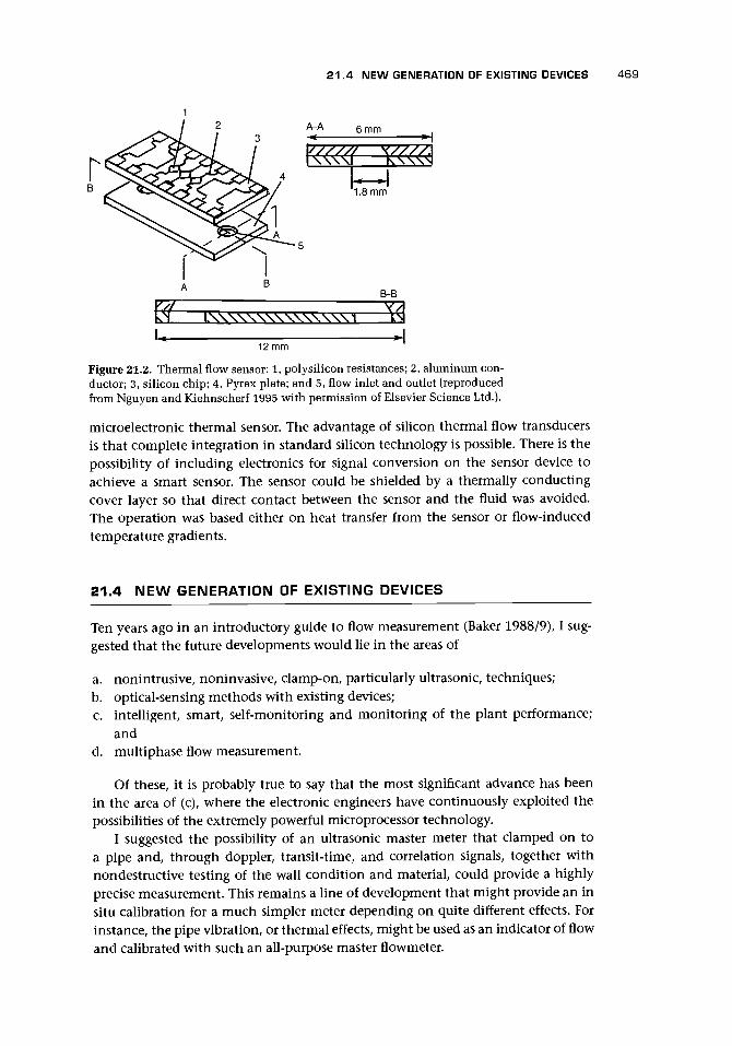
21.4 NEW GENERATION OF EXISTING DEVICES 469
2 A~A 6 mm3 ^
ys///( VWV31.8 mm
B-B
12 mm
Figure 21.2. Thermal flow sensor: 1, polysilicon resistances; 2, aluminum con-ductor; 3, silicon chip; 4, Pyrex plate; and 5, flow inlet and outlet (reproducedfrom Nguyen and Kiehnscherf 1995 with permission of Elsevier Science Ltd.).
microelectronic thermal sensor. The advantage of silicon thermal flow transducersis that complete integration in standard silicon technology is possible. There is thepossibility of including electronics for signal conversion on the sensor device toachieve a smart sensor. The sensor could be shielded by a thermally conductingcover layer so that direct contact between the sensor and the fluid was avoided.The operation was based either on heat transfer from the sensor or flow-inducedtemperature gradients.
21.4 NEW GENERATION OF EXISTING DEVICES
Ten years ago in an introductory guide to flow measurement (Baker 1988/9), I sug-gested that the future developments would lie in the areas of
a. nonintrusive, noninvasive, clamp-on, particularly ultrasonic, techniques;b. optical-sensing methods with existing devices;c. intelligent, smart, self-monitoring and monitoring of the plant performance;
andd. multiphase flow measurement.
Of these, it is probably true to say that the most significant advance has beenin the area of (c), where the electronic engineers have continuously exploited thepossibilities of the extremely powerful microprocessor technology.
I suggested the possibility of an ultrasonic master meter that clamped on toa pipe and, through doppler, transit-time, and correlation signals, together withnondestructive testing of the wall condition and material, could provide a highlyprecise measurement. This remains a line of development that might provide an insitu calibration for a much simpler meter depending on quite different effects. Forinstance, the pipe vibration, or thermal effects, might be used as an indicator of flowand calibrated with such an all-purpose master flowmeter.

470 FUTURE DEVELOPMENTS
Optical methods have clearly moved on substantially in 10 years, although theirdirect use in process sensors is an area for further development. With Morris (1983),I reviewed the suitability of flowmeters for optical sensing, and more recently Dick-inson (1988) considered design of optical flowmeter sensors. His paper has examplesof variable area, turbine, thermal, and cross correlation. Dickinson suggested that anoninvasive pickup to sense rotation in turbine and positive displacement withoutany moment/movement would be useful, as would the development of a vortexmeter using optical methods for steam.
I have already commented on the needs for more development in the area ofmultiphase, particularly subsea, flows.
The new areas that I would add to the preceding list are
• Mass meters for gases. I have already referred to this and suspect that it liesin the improvement of thermal and ultrasonic methods, possibly linked to-gether.
• Microsensors. Here the possibilities appear to be very exciting and, if used asbypass flowmeters, very extensive.
21.5 IMPLICATIONS OF INFORMATION TECHNOLOGY
21.5.1 SIGNAL ANALYSIS
The idea that the signal, far from being smoothed, contains data that can revealinformation about the meter and the process (Amadi-Echendu and Higham 1990,Amadi-Echendu and Hurren 1990) is an important insight. It suggests that thenoise may carry a fingerprint of the meter and may be interpreted by powerfulcomputational methods to indicate change, possibly correction factors and indeedmany other factors. However, if this is to be fully realized, it is essential that modelslinking the flowmeter/flow system behavior with the noise characteristics bedeveloped, to give a firm theoretical basis. Cheesewright et al. (1998) have providedan appropriate caution.
21.5.2 REDESIGN ASSUMING MICROPROCESSOR TECHNOLOGY
An intriguing question to ask is: what would have been the design of flowmeters,which are now dominated by mechanical engineering, if the power of the micro-processor had been available? For instance, the "fingerprint" of the vibration of apipe might be stored in the microprocessor for various flow rates and be used as alook-up table, but the actual sensor might be a simple vibration sensor.
21.5.3 CONTROL
There seems little doubt that the extraordinary developments in control, and theincreasing flexibility will continue in the next 10 years or more.
For instance, by collecting data on correct plant operation, together with modelsof the plant flows, and by checking current flows against the data and model, anyplant changes (e.g., occurrence of leaks) can be identified (Valenti 1995).

21.7 THE WAY AHEAD 471
21.5 .4 RECORDS, MAINTENANCE, AND CALIBRATIONYeung et al. (1994) reported on a detailed survey of the use of insertion meters incollaboration with four water utilities and six consultancy companies in the UnitedKingdom. There were deficiencies in records, equipment maintenance and calibra-tion, work instructions, and training. There was also a difference in perception be-tween management and the technicians, and an ignorance about the ownership andmaintenance of records.
There is clearly a need for training in essential information such as standarddocuments and their requirements. This is an area where modern information andcommunication methods, particularly linked with modern control, should ensurethat much documentation is automatically produced. Gallagher (1992) also raisedthe issue of certification of technicians.
21.6 CHANGING APPROACHES TO MANUFACTURINGAND PRODUCTION
This book has not pretended to give guidance in the area of manufacturing andproduction. However, a key change in recent thinking has been the use of cell man-ufacture and the consequent increase of ownership and responsibility by the teamin the cell. In the area of instrumentation, I have suggested that there is room forcareful understanding of the links between production methods and instrument ac-curacy. It is an area where precise measurement of the production process, and ofthe product as it moves through the process, is needed and where new methods arelikely to be developed.
21.7 THE WAY AHEAD
21.7.1 FOR THE USERThe competition in the market place is fierce, and the products vary in performanceand quality. Time spent, and advice sought, on the best device for a particular ap-plication may save much time and money in the next 10 years.
21.7.2 FOR THE MANUFACTURERThe ability to tailor the product to the user's needs, the opportunity for the user tosend an order by modern communication (e-mail, etc.), and the ability to deliverthis special order in days or even hours, is possible, and some manufacturers areachieving remarkable order-to-delivery times. Staying in business requires that stepsbe taken to achieve this. In the process, it is likely to lead to the rethinking of manyaspects of production to the benefit of the company, and if all the work force isinvolved, to their benefit also.
21.7.3 FOR THE INCUBATOR COMPANYNew start-up companies run by an entrepreneur with a brilliant new concept areto be encouraged, but in this competitive market, they will need support. Suchsupport exists and is likely to be more widely available as time passes. At its best,

472 FUTURE DEVELOPMENTS
it may provide space on a relatively low rent and for a manageable forward timecommitment, advice on legal and other matters, advice on financial needs, andpossibly training in the manufacturing, management, finance, and marketing areaswith which a scientist/inventor may be less familiar.
21.7.4 FOR THE R&D DEPARTMENT
This book has brought much of the literature together, but I would not pretend thatit is remotely exhaustive. The R&D department will need to work with the wholecompany to coordinate the new product needs. However, from the other side, theavailability of exhaustive literature searches to find new ideas, should raise manypossibilities. Developments in the science base should also be explored, and jointprojects should be initiated. Collaboration with the science base can be mutuallybeneficial, providing the industrial partner stays the course and is not put off by thevery different culture, particularly of the university research interface.
21.7.5 FOR THE INVENTOR/RESEARCHER
The power of modern microprocessing and micromechanics suggests that a freshlook should be taken at every flow measurement application to see if extremelysimple sensors can provide signals capable of interpretation.
21.8 CLOSING REMARKS
Flow measurement is a large and varied subject. It uses almost every area of classicalphysics in the many and varied sensors. It attempts to measure mean flows in pipesdownstream of complex pipework. It attempts to cope with highly adverse condi-tions both of fluid and of environment. From long experience, I have found thatmost of the questions posed in industrial workshops are unanswerable, and that thesolutions to the questions would merit a major research program.
It is also an increasingly competitive field for the manufacturer, in which anysort of collaboration is viewed with suspicion. It is, therefore, refreshing to findLetton (1994) making a plea for cooperation in product development in this hightechnology industry.
There is, however, a role for the science base, in terms of the development of newdevices, the application of more sophisticated signal processing, and the assemblyof even more powerful control techniques.
There is another area where the leading university groups can bring a fresh insightand an on-going collaboration. Those who develop their expertise in the operationof industry can provide an independent and critical view on the modernization ofthe whole production function: to reduce waste, to improve quality control, to placemore responsibility and initiative on the production cell, to improve the automaticacquisition of documentation on the product flow, and to improve responsivenessand speed of delivery to the customer.
I hope that this book will provide a significant contribution, firstly to the fulfil-ment of those people whose work is with flowmeters, from invention to application;secondly to the quality of the product; and thirdly to the financial success of the en-terprises, so that the industrial flows of fluids of all sorts will, as a result, be measuredmore precisely and reliably.

Bibliography
The list of books on flow measurement is lengthy, and I am sure that this one is not complete,but it represents those books that I have come across. That they are included here is neither arecommendation nor otherwise. Each author provides a particular emphasis: practical, theo-retical, fluid, bulk measurement, probes, anemometry.
Baker, R. C. (1988/9) An Introductory Guide to Flow Measurement. London: Mechanical Engineer-ing Publications.
(1996) An Introductory Guide to Industrial Flow. London: Mechanical Engineering PublicationsLtd.
Benard, C. J. (1988) Handbook of Fluid Flowmetering. Morden, England: The Trade & TechnicalPress.
BS 7405 (1991) Guide to the Selection and Application ofFlowmeters. London: British StandardsInstitution.
Cascetta, R, and Vigo, P. (1988) Flowmeters - A Comprehensive Survey and Guide to Selection.Research Triangle Park, NC: ISA Publishing.
Cheremisinoff, N. P., and Cheremisinoff, P. N. (1988) Flow Measurement for Engineers and Scien-tists. New York: Marcel Dekker.
Danen, G. W. A. (Ed.) (1985) Shell Flowmeter Engineering Handbook, 2nd ed. New York: McGraw-Hill.
DeCarlo, J. P. (1984) Fundamentals of Flow Measurement. Instrument Society of America.Endress and Hauser (1989) Flow Handbook. Switzerland: Flowtec AG (English edition).Fowles, G. (1993) Flow Level and Pressure Measurement in the Water Industry. Butterworth
Heinneman. (Series editor B. E. Noltingk in association with the Institute of Measurementand Control).
Furness, R. A. (1989) Fluid Flow Measurement. Harlow U. K. Longman. (In association with TheInstitute of Measurement and Control.)
Furness, R. A., and Heritage, J. E. (1989) The Redwood Flowmeter Directory. London: IBC TechnicalServices.
Hayward, A. T. J. (1977) Repeatability and Accuracy. London: Mechanical Engineering Publica-tions.
(1979) Flowmeters: A Basic Guide and Source Book for Users. London: Macmillan.Hogrefe, W., Kirchof, U., Mannherz, E., Marchewka, W., Mecke, U., Otto, E, Rakebrandt, K.-H.,
Thone, A., and Wegener, H.-J. (1995) Guide to Flowmeasurements. Gottingen: Bailey-Fischer& Porter GmbH.
Jones, F. E. (1995) Techniques and Topics in Flow Measurement. New York: CRC Press.Linford, A. (1961) Flow Measurement & Meters, 2nd ed. London: E. & F. N. Spon.Miller, R. W. (1996) Flow Measurement Engineering Handbook, 3rd ed. New York: McGraw-Hill.Noltingk, B. E., Ed. (1988) Instrumentation Reference Book. London: Butterworths.Ower, E., and Pankhurst, R. C. (1966) The Measurement of Air Flow, 4th ed. London: Pergamon
Press.Scott, R. W. W., Ed. (1982) Developments in Flow Measurement - 1. London: Applied Science
Publishers.Shercliff, J. A. (1962) The Theory of Electromagnetic Flow-Measurement. Cambridge: Cambridge
University Press.
473

474 BIBLIOGRAPHY
Spink, L. K. (1978) Principles and Practice of Flow Meter Engineering, 9th ed. Foxboro MA : TheFoxboro Co.
Spitzer, D. W. (1990) Industrial Flow Measurement. Instrument Society of America.Spitzer, D. W.; Ed. (1991) Flow Measurement. Instrument Society of America.Upp, E. L. (1993) Fluid Flow Measurement. Houston: Gulf Publishing.

A Selection of International Standards
In most cases I have omitted full details and directed the reader to the documentname or number. This is partly for conciseness and partly because continual updateresults in new dates for the standards.
Organizations involved in the development of standards include: InternationalStandards Organization (ISO), International Electrotechnical Commission (IEC), Or-ganisation International de Metrologie Legale (OIML), American Gas Association(AGA), American National Standards Institute (ANSI), American Petroleum Institute(API), American Society of Mechanical Engineers (ASME), British Standards Insti-tution (BSI), CEN/CENELEC European Standards, Institute of Petroleum (IP), andInstrument Society of America (ISA).
GeneralISO 4006:1991 Measurement of fluid flow in closed conduits - Vocabulary and symbols,Bilingual edition (BS 5875).
See also ASME MFC-1M-(R1986)
UncertaintyISO 5168:1978 Measurement of fluid flow - Estimation of uncertainty of a flow-ratemeasurement (BS 5844).
See also ISO/DIS 11631 and ASME MFC-2M-(R1988)
SelectionBS 7405:1991 Guide to selection and application of flowmeters for the measurement offluid flow in closed conduits. AMD 8879 (1995).
CalibrationISO 4185:1980 Measurement of liquid flow in closed conduits - Weighing method(BS 6199-1).
ISO 7278 Liquid hydrocarbons - dynamic measurements. Proving systems for volumetricmeters (BS 6866).
ISO 8316 Measurement of liquid flow in closed conduits using weighing and volumet-ric methods. Method for measurement by collection of the liquid in a volumetric tank(BS 6199).
ISO 7066 Assessment of uncertainty in calibration and use of flow measurement devices.
ISO 8222 Petroleum measurement systems - Calibration - Temperature corrections for usewith volumetric reference measuring systems.
475

476 A SELECTION OF INTERNATIONAL STANDARDS
ISO 8316 Measurement of liquid flow in closed conduits - Method by collection of theliquid in a volumetric tank (BS 6199-2).
ISO 9368 Measurement of liquid flow in closed conduits by the weighing method.
In situ VerificationISO 2975 Measurement of water flow in closed conduits - Tracer methods (BS 5857).
ISO 3354 Measurement of clean water flow in closed conduits - Velocity-area method usingcurrent-meters in full conduits and under regular flow conditions.
ISO 3966 Measurement of fluid flow in closed conduits - Velocity area method using Pitottubes (BS 1042-2.1).
ISO 4053 Measurement of gas flow in conduits - Tracer methods (BS 5857-2.1).
ISO 7194 Measurement of fluid flow in closed conduits - Velocity-area methods of flowmeasurement in swirling or asymmetric flow conditions in circular ducts by means ofcurrent-meter or Pitot static tubes (BS 1042-2.3).
See also IP publications on proving
Orifice, Venturi, and NozzlesISO 5167-1:1997 Specification for square-edged orifice plates, nozzles and venturi tubesinserted in circular cross-section conduits running full. (BS 1042 Section 1.1).
ISO 2186 Fluid flow in closed conduits - Connections for pressure signal transmissionsbetween primary and secondary elements.
ISO/TR 3313 Measurement of pulsating flow in a pipe by means of orifice plates, nozzlesor venturi tubes (in particular in the case of sinusoidal or square wave intermittentperiodic-type fluctuations).
See also BS 1042, API Manual of Petroleum Measurement Standards Chapter 14.3,ASME MFC-3M-1989, etc.
Critical Flow Venturi Nozzles9300:1990 Measurement of gas flow by means of critical flow venturi nozzles.
ANSI/ASME MFC-6M-1987 Measurement of gas flow by means of critical flow venturinozzles.
Variable AreaBS ISO 11605:1995 Paper and board. Calibration of variable-area flowmeters.
Positive Displacement MetersISO 2714 Liquid hydrocarbons - Volumetric measurement by displacement meter systemsother than dispensing pumps.
See BS for information on diaphragm meters and rotary displacement meters forgas. See also IOML.

A SELECTION OF INTERNATIONAL STANDARDS 477
Turbine MetersISO 2715 Liquid hydrocarbons - Volumetric measurement by turbine meter systems.
ISO 9951 Measurement of gas flow in closed conduits - Turbine meters.
ANSI/ASME MFC-4M-1986 Measurement of gas flow by turbine meters.
AG A Measurement of fuel gas by turbine meters, Transmission Measurement CommitteeReport, No 7.
ANSI/ISA RP31.1 Recommended practice specification, installation and calibration of tur-bine flowmeters.
ANSI/API 2534 Measurement of liquid hydrocarbons by turbine meter systems.
Vortex MetersISO/TR 12764:1997 Measurement of fluid flow in closed conduits - Flowrate measurementby means of vortex shedding flowmeters inserted in circular cross-section conduits runningfull.
Electromagnetic FlowmetersISO 6817:1997 Measurement of conductive liquid flow in closed conduits. Method usingelectromagnetic flowmeters.
ISO 9104:1991 Measurement of fluid flow in closed conduits - Methods of evaluating theperformance of electromagnetic flowmeters for liquids.
Ultrasonic FlowmetersISO/TR 12765:1998 Methods using ultrasonic transit-time flowmeters.
AGA Transmission Measurement Committee Report No 9, Measurement of gas bymultipath ultrasonic meters, June 1998.
ASME MFC-5M-1985 Measurement of liquid flow in closed conduits using transit-timeultrasonic flowmeters.
See also BS 4331 and VDE/VDI
Thermal Mass FlowmetersISO/CD-14511:1998 Measurement of fluid flow in closed conduits - Thermal massflowmeters.
Coriolis FlowmetersISO 10790:1998(E) Measurement of fluid flow in closed conduits - Coriolis massflowmeters.
ProbesISO 3966 Method using pitot-static tubes.
ISO 7145 Determination of flowrate of fluids in closed conduits of circular cross-section -Method of velocity measurement at one point of the cross-section (BS 1042-2.2).

478 A SELECTION OF INTERNATIONAL STANDARDS
Modern Control SystemsISO 7498-1:1995 Information technology open systems interconnection basic referencemodel.
Some Other Industry-Specific StandardsPetroleum
API Manual of Petroleum Measurement Standards and other API documents.
Water
ISO 4064 Measurement of flow in closed conduits.
BS 5728 Flow of cold potable water in closed conduits.
ISO 7858 Measurement of water flow in closed conduits.
ANSI/AWWA (American Water Works Association) documents.
GasANSI/CGA (Compressed Gas Association) documents.
ANSI/UL (Underwriters Laboratories) documents.
Road Vehicle Testing
ISO 7440 Road vehicles - Fuel injection equipment testing.
(Sources used to compile this list are: ISO and BS indexes, Institute of Measurementand Control Yearbook 1998, Upp 1993).

Conferences
This list does not include some of the major professional institution conferences ofwhich flow measurement is a part, and that are run by ASCE, ASME, ISA, AGA, etc.Nor does it include all the conferences that impinge on flow measurement but thatcover much wider areas and for which it is not necessarily central (e.g., Gas ResearchConferences).
Proceedings of a Symposium on Flow Measurement in Closed Conduits, NationalEngineering Laboratory, Scotland, 1962.Institute of Measurement & Control Symposium on the Measurement of PulsatingFlow: 1970.Proceedings of the International Conference on Modern Developments in Flow Mea-surement, England: Harwell (Published 1972 by Peter Peregrinus Ltd.), 1971.Fluid Dynamics Measurements (from Fluids Engineering Conference, Pittsburgh, PA,and Winter Annual Meeting, Washington, DC), ASME Fluids Division, 1971.Conference on Fluid Flow Measurement In The Mid 1970;s, Scotland: NationalEngineering Laboratory, 1975.FLO-CON 11 Proceedings of the Symposium - The Application of Flow MeasuringTechniques, Brighton, UK: 1977.FLOMEKO 1978 - Flow Measurement of Fluids, North Holland, Amsterdam: 1978.Proceedings Transducer 11 Conference Flow Measurement Session, Wembley,London, 1977.Measurement in Polyphase Flows, Winter Annual Meeting, ASME Fluids EngineeringDivision, San Francisco, CA, 1978.NEL Fluid Mechanics Silver Jubilee Conference, East Kilbride, Glasgow, Scotland:1979.Flow, Its Measurement and Control in Science and Industry, Flow 81 Conference,St Louis, ISA, 1981. (Three volumes)International Conference on Advances in Flow Measurement Techniques, Coventry,England, 1981.BHRA Conference on Physical Modelling of Multi Phase Flow, Coventry, 1983.Conference on Flow Metering and Proving Techniques in the Offshore Oil Industry,Aberdeen, 1983.International Gas Research Conference, London, 1983.
479

480 CONFERENCES
International Conference on the Metering of Natural Gas and Liquefied HydrocarbonGases, London, 1984.64th Annual GPA Convention, Houston, Texas, 1985.International Conference on the Metering of Petroleum and its Products, OYEZ,London, 1985.Conference on Fluid Control and Measurement, Tokyo, Japan, 1985.Flow Measurement for Water Supply, London, 1985.Second International Conference on Multi-phase Flow, London: BHRA, 1985.International Conference on Flow Measurement in the Mid 80;s, 9-12 June.Glasgow: NEL, 1986.International Symposium on Fluid Flow Measurement, Washington, DC, 1986.Trends in Instrumentation - Signal processing for flow measurement PC-based in-strumentation systems, IOP Short Series No. 5 in collaboration with Trident Inter-national Exhibitions Limited, 25th February 1987.Second International Conference on Flow Measurement, BHRA, London, 1988.FLUCOME '88, H S Stephens & Associates, Sheffield, September 1988.North Sea Metering Workshop, National Engineering Laboratory, East Kilbride,Scotland, 1988. (This series started in 1983 in Stavanger, Norway.)FLOMEKO '89 - Fifth International Conference on Flow Measurement, Dusseldorf,Germany, 1989.Multiphase Flow - Proceedings of the Fourth International Conference, BHRA,Cranfield, 1989.North Sea Flow Measurement Workshop, Haugesund, Norway, 1989.Second International Symposium on Fluid Flow Measurement, Calgary, Alberta,Canada, June, 1990.International Conference on Flow Measurement of Commercially Important Fluids,London, England, 1990.North Sea Flow Measurement Workshop, National Engineering Laboratory, Scotland,1990.Advanced Techniques for Integrated Circuit Processing, International Society OpticalEngineers, Proceedings of SPIE, 1990/91.FLUCOME '91, Proceedings of the 3rd Triennial International Symposium on FluidControl, ASME, Measurement and Visualization, San Francisco, Cal, USA, 1991.North Sea Flow Measurement Workshop, Norwegian Society of Chartered Engineers,1991.International Conference on Flow Measurement in Industry and Science, London,1991.North Sea Flow Measurement Workshop, National Engineering Laboratory, Scotland,1992.Annual Symposium on Instrumentation for the Process Industries, Texas, 1992.FLOMEKO ;93 - Sixth International Conference on Flow Measurement, Korea, 1993.North Sea Flow Measurement Workshop, Bergen, Norway, 1993.

CONFERENCES 481
Flow Measurement for the Utilities, Amsterdam, The Netherlands, 4-5 Nov. 1993.Sponsored by /. Flow Meas. Instrum.FLOMEKO ;94 - International Conference on Flow Measurement in the Mid 90's,Glasgow, Scotland, June 1994.FLUCOME '94, Toulouse, France, 1994.North Sea Flow Measurement Workshop, Peebles, Scotland, 1994.ISA Advances in Instrumentation and Control: International Conference and Exhi-bition, 1995.North Sea Flow Measurement Workshop, National Engineering Laboratory, Scotland,1995.Advances in Instrumentation and Control: International Conference and Exhibition(ISA), 1996.FLOMEKO '96 - Eighth International Conference on Flow Measurement, Beijing,China, 1996.North Sea Flow Measurement Workshop, Peebles, Scotland, 1996.Symposium on Flow in Open Channels and Closed Conduits, Gaithersburg, MD,1997.North Sea Flow Measurement Workshop, Kristiansand, Norway, 1997.FLOMEKO '98 - Ninth International Conference on Flow Measurement, Lund,Sweden, 1998.North Sea Flow Measurement Workshop, Gleneagles, Scotland, 1998.


References
Abe, J., and Yoshinaga, A. (1991) Flowmeasurement by using fluidic resistor. FLUCOME '91 3rdTriennial Int. Symp. on Fluid Control, Measurement and Visualization. San Francisco: 559-564.
Abernathy, F. H.; and Kronauer, R. E. (1962) The formation of vortex streets. /. Fluid Mechanics,13:1-20.
Adiletta, G., Cascetta, F.; della Valle, S.; Pagano, S., and Vigo, P. (1993) Twin rigid straight pipeCoriolis mass flowmeter. Measurement, 11:289-308.
Advisory Committee on Aeronautics (1916-17) Reports and Memoranda, No. 295:675.AGA-8 (1992) Compressibility and supercompressibility for natural gas and other hydrocarbon
gases, Transmission Measurement Committee Report No. 8, AGA Catalog No. XQ 1285,Arlington, VA.
Agarwal, A. K., and Turgeon, M. (1984) New MicroMotion mass flowmeters. Energy Progr. 4:221-224.
Agricola, J. B. (1997) Gas well flowline measurement by ultrasonic flow meter. North Sea FlowMeasurement Workshop, Kristiansand, Norway, Paper 16.
Ahmad, K., Baker, R. C, and Goulas, A. (1986) Computation and experimental results of wearin a slurry pump impeller. Proc. I. Mech. E, Pt. C, 200:439-445.
Al-Asmi, K., and Castro, I. P. (1992) Vortex shedding in oscillatory flow: Geometrical effects./. FlowMeas. Instrum., 3:187-202.
Al-Khazraji, Y. A., Al-Rabeh, R. H., Baker, R. C, and Hemp, J. (1978) Comparison of the effectof a distorted profile on electromagnetic, ultrasonic and differential pressure flowmeters,FLOMEKO 1978 - Proc. Conf. on Flow Measurement of Fluids. Groningen, The Netherlands(Amsterdam: North-Holland Publishing Co.): 215-22.
Al-Khazraji, Y. A., and Baker, R. C. (1979) Analysis of the performance of three large-electrodeelectromagnetic flowmeters. /. Phys. D, 12:1423-34.
Al-Khazraji, Y. A., and Hemp, J. (1980) Electromagnetic flowmeters and methods of measuring flow.U.S. Patent 4,434,666, March 6, 1984 (filed April 4, 1980).
Allen, C. (1994) The Interoperable Systems Project (ISP). Meas. Control, 27(2):38-41.Al-Rabeh, R. H. (1981) The theory and performance of electromagnetic flowmeters. PhD Thesis,
Imperial College, University of London, England.Al-Rabeh, R. H., and Baker, R. C. (1979) Optimisation of conventional electromagnetic flowme-
ters. Fluid Mechanics Silver Jubilee Conference, National Engineering Laboratory, Glasgow,Scotland, Paper 6.1.
(1986) On the ability to dry calibrate an electromagnetic flowmeter. /. Phys. E: Sci. Instrum.,19:203-206.
Al-Rabeh, R. H., and Hemp, J. (1981) A new method for measuring the flow rate of insulatingfluids. Int. Conf on Advances in Flow Measurement Techniques, BHRA, Paper K3:267-278.
Al-Rabeh, R. H., Baker, R. C, and Hemp, J. (1978) Induced flow measurement theory for poorlyconducting fluids. Proc. Roy. Soc. A, 361:93-107.
Aly, F. A., and Lee, L. L. (1981) Self consistent equations for calculating the ideal gas heatcapacity, enthalpy and entropy. Fluid Phase Equilibria, 6:169-179.
Amadi-Echendu, J. E., and Higham, E. H. (1990) Additional information from flowmeters viasignal analysis. IEEE Trans. Instrum. Meas., 39(6):998-1003.
Amadi-Echendu, J. E., and Hurren, P. J. (1990) Identification of process plant signatures usingflow measurement signals. IEEE Trans. Instrum. Meas., 39(2):416-20.
483

484 REFERENCES
Amadi-Echendu, J. E.; and Zhu, H. (1992) Signal analysis applied to vortex flowmeters. IEEETrans. lustrum. Meas., 41(6):1001-4.
Amadi-Echendu, J. E.; Zhu, H., and Higham, E. H. (1993) Analysis of signals from vortex flowme-ters. /. Flow Meas. Instrum., 4:225-32.
Amini, A.; and Owen, I. (1995) The use of critical flow venturi nozzles with saturated wet steam./. Flow Meas. Instrum., 6:41-7.
Anon. (1966a) Measuring beefeater gin. Control, 10(96):292.(1966b) Positive displacement flowmeter for low rates. Control, 10(98):437.(1988) NEL launches offshore multiphase flowmeter project. Process Eng., October: 33.(1993) Non-intrusive multiphase flow meter. Offshore Research Focus, No. 98:9.(1994) Multiphase flow meter. Offshore Research Focus, No. 103:2.
ANSI/API 2530:1985 Orifice metering of natural gas and other related hydrocarbon fuels.Aoki, T., Nukui, K., Okamura, S., and Kimura, Y. (1996) Development of fluidic gas meter
(improvement of sensitivity at lower flow rate using U-shaped target sensor), FLOMEKO'96Proc. 8th Int. Conf. on Flow Measurement, Beijing, China: 138-43.
API (1992) American standard method for measurement of liquid hydrocarbons by displace-ment meter systems, Chapter 5.2, Manual of Petroleum Measurements. Washington DC:American Petroleum Institute.
Arasi, J. A. (1989) Coriolis mass flowmeter passes NGL line field trials. Oil & Gas /., January:59-61.
Arnberg, B. T., Britton, C. L., and Seidl, W. F. (1973) Discharge coefficient correlations forcircular-arc venturi flowmeters at critical (sonic) flow. ASME, Paper No 73-WA/FM-8.
Arnold, R. M., and Pitts, R. W. (1981) Fluid flow meters for mixed liquid and gas. U.S. Patent4,272,982, June 16.
Aschenbrenner, A. (1989) Calibration of the new test rig for large gas meters of the Physikalisch-Technische Bundesonstalt. FLOMEKO 5th Int. Conf on Flow Measurement: 11-22.
Asher, R. C. (1983) Ultrasonic transducers for chemical and process plant. Phys. Technol, 14:19-23.
(1997) Ultrasonic Sensors: For Chemical and Process Plant. Bristol, UK: Institute of Physics.ASME/ANSI MFC-7M (1987) Measurement of gas flow by means of critical flow venturi nozzles.
New York: ASME.Aston, N. A. J., and Evans, G. V. (1975) The integrated pulse velocity method applied to the cali-
bration of flowmeters in high pressure natural gas systems. Conf. on Fluid Flow Measurementin the Mid 1970's, Paper D-2, East Kilbride, Scotland: National Engineering Laboratory.
Athane, B. (1994) Implications of legal metrology in flow measurement for the utilities. /. FlowMeas. Instrum., 5(2):67-9.
Atkinson, K. N. (1992) A software tool to calculate the over-registration error of a turbine meterin pulsating flow. /. Flow Meas. Instrum., 3:167-172.
Awberry, J. H., and Griffiths, E. (1926-7) Further experiments with the Ewing ball-and-tubeflowmeter. Proc. Roy. Soc, Edinburgh, 47:1.
Baird (1993) Innovations in magnetic flowmetering. Advances in Instrumentation and Control:Int. Conf. Exhib. (ISA), Chicago, 48:879-84.
Baker, P. D. (1983) Positive displacement liquid meters. International School of Hydrocarbon Mea-surement (ISHM), University of Oklahoma, April 12-14.
Baker, R. C. (1968) Solutions of the electromagnetic flowmeter equation for cylindrical geome-tries. Brit. J. Appl. Phys. (J. Phys. D), l(2):895-9.
(1969) Flow measurement with motion induced magnetic field at low magnetic Reynoldsnumber. Magnetohydrodynamics, 3:69-73 (in Russian).
(1970a) Effects of non-uniform conductivity fluids in electromagnetic flowmeters. /. Phys. D,3:637-9.
(1970b) Linearity of motion-induced-magnetic-field flowmeter. Proc. I.E.E., 117:629-33.(1973) Numerical analysis of the electromagnetic flowmeter. Proc. I.E.E., 120:1039-43.(1976) Some recent developments in ultrasonic and electromagnetic pipe flow measurement
at Imperial College. ACTAIMEKO VII: 339-48.(1977) Liquid metal electromagnetic flowmeters in fast reactor technology. Prog. Nucl. Energy,
1:41-61.(1982) Electromagnetic flowmeters, pp. 209-51. Developments in Flow Measurement - 1 (R. W.
W. Scott, Ed.), London: Applied Science Publishers Ltd.
REFERENCES 485
(1983) A review of recent developments in electromagnetic flowmeasurement. Third Beer-Sheva Seminar on MHD - Flows and Turbulence, Ben-Gurion University of the Negev, Beer-Sheva, Israel, 23-27 March 1981. Also in Prog. Astro. Aero., 84:225-59.
(1985) Principles and Practice of electromagnetic flowmeasurement. Technisches Messen,52(1):4-12 (in German).
(1988) Measuring multiphase flow. Chem. Engineer, October: 39-45.(1988/9) An Introductory Guide to Flow Measurement. London: Mechanical Engineering Publica-
tions.(1989) Multi-phase flow moves on. Control Instrum., February: 35, 37.(1991a) Response of bulk flowmeters to multiphase flow. Proc. I. Mech. E. Part C: J. Mech. Eng.
Sci., 205:217-29.(1991b) Turbine and related flowmeters: Part I - Industrial practice. /. Flow Meas. Instrum.
2:147-62.(1993) Turbine flowmeters: Part II - Theoretical and experimental published information. /.
Flow Meas. Instrum., 4:123-44.(1996) An Introductory Guide to Industrial Flow. London: Mechanical Engineering Publications.(1998) Flowmeter, pp. 245-7. Instruments of Science, An Historical Encyclopedia (R. Bud and
D. J. Warner, Eds.), New York and London: Garland Publishing Inc.Baker, R. C, and Deacon, J. E. (1983) Tests on turbine, vortex and electromagnetic flowmeters in
2-phase air-water upward flow. Int. Conf. on Physical Modelling ofMulti-Phase Flow, Coventry,England, BHRA Fluid Engineering, Paper HI: 337-52.
Baker, R. C, and Hayes, E. R. (1985) Multiphase measurement problems and techniques forcrude oil production systems. Petrol. Rev., November: 18-22.
Baker, R. C, and Higham, E. H. (1992) Flowmeters. U.K. Patent 2 231 669 B, December 23.Baker, R. C, and Morris, M. V. (1983) The suitability of flowmeters for optical techniques.
Proc. Int. Conf. on Optical Techniques in Process Control. The Hague, Netherlands (Cranfield,England: BHRA) (post-deadline paper).
(1985) Positive-displacement meters for liquids. Trans. Inst. M.C., 7:209-20.Baker, R. C, and Smith, D. J. M. (1990) Flowmeter Specification Guidelines, Report No. 14.
Cranfield, England: FLOMIC.Baker, R. C, and Tarabad, M. (1978) The performance of electromagnetic flowmeters with
magnetic slurries. /. Phys. D, 11:167.Baker, R. C, and Thompson, E. J. (1975) A two beam ultrasonic phase-shift flowmeter. Conf.
on Fluid Flow Measurement in the Mid 1970s, East Kilbride Glasgow, Scotland: National En-gineering Laboratory.
(1978) Measurement of fluid flow, U.S. Patent 4,078,428, March 14.Baker, R. C, Deacon, J. E., Lenn, C. P., and Smart, M. D. (1985) The effect on electromagnetic
flowmeters of a change in fluid. Meas. Control, 8:5-10.Ball, J. M. (1977) Viscosity effects on the turbine flowmeter. Proc. Symp. on Flow Measurement in
Open Channels and Closed Conduits. NBS, Gaithersburg, MD: 847-69.Balls, B. W., and Brown, K. J. (1959) The magnetic flowmeter. Symp. on Flow Measurement: Trans.
Soc. Instrument Technology, June: 123-30.Barnes, R. G. (1982) Positive displacement liquid meters. Adv. Instrum., 37(3):1197-204. Proc.
ISA. Int. Conf. Exhib., (Philadelphia, PA, USA, 18-21 October 1982), Research Triangle Park,USA, Instrum Soc Am.
Barry, J. J., Sheikoleslami, M. Z., and Patel, B. R. (1992) Numerical simulation of flow throughorifice meters, Gas Research Institute, GRI-92/0060.1.
Batchelor, G. K. (1967) An Introduction to Fluid Dynamics. Cambridge: Cambridge UniversityPress.
Bates, C. J. (1981) Laser doppler anemometry measurements of the flow through an orificeplate. Flow Its Measurement and Control in Science and Industry, 2:59-68.
Bates, I. P. (1991) Field use of K-lab flow conditioner. Proc. North Sea Flow Measurement Workshop1991 (two volumes), Norwegian Society of Chartered Engineers, October 22-24, 1991 (9thin the series).
Battye, J. S. (1993) The correlation flowmeter - A detailed investigation of an attempt to improveits performance. FLOMEKO '93 Proc. 6th Int. Conf. on Flow Measurement, Korea: 492-499.
Baucom, W. E. (1979) Evaluation of a coriolis mass flow meter for pulverized coal flows. Pre-pared by The Energy Conservation Division, The University of Tennessee Space Institute,

486 REFERENCES
Tullahoma, Tennessee 37388, for the U.S. Dept. Energy (Contract No. DE-AC02 -79ET10815, December).
Baumoel, J. (1994) Use of clamp-on transit-time ultrasonic flowmeters in Aircraft mass fuelflow, hydraulic fluid leak detection, & ground support applications. Instrumentation in theAerospace Industry: Proc. Int. Symp. ISA, Research Triangle Park, NC: 243-60.
(1996) Pipeline management using networked clamp-on transit-time flowmeters. Proc. Int.Pipeline Conf., Calgary, Canada, New York: ASME, Vol. 2:1123-8.
Bean, H. S. (1971) Fluid Meters, Their Theory and Application, 6th ed. New York: ASME.Beck, M. S., and Plaskowski, A. (1987) Cross Correlation Flowmeters - Their Design and Application.
Bristol, UK: Adam Hilger.Beeson, J. (1995) Ultrasonics meters improve NorAm's custody transfer. Pipeline & Gas J.,
222(7):21-4.Beg, N., and Toral H. (1993) Off-site calibration of a two-phase pattern recognition flowmeter.
Int. J. Mult. Flow, 19:999-1012.Bellinga, H., and Delhez, F. J. (1993) Experience with a high-capacity piston prover as a primary
standard for high-pressure gas flow measurement. /. Flow Meas. Instrum., 4:85-90.Bellinga, H., and Stronk, H. B. (1974) The practical application of flow straighteners with turbine
flowmeters for gas. IMEKO VII Conf., London, Paper BFL/242:1-11.Bellinga, H. Hoek, C. P., Kooi, A., Van Laak, F. A. L, and Orbous, P. J. (1981) Using a piston prover
as a primary standard in high-pressure gas metering. Flow, Its Measurement and Control inScience and Industry, Flow '81 Conference, St Louis, ISA.
Benabdelkarim, M., and Galiana, C. (1991) Nonradioactive densitometer for continuous mon-itoring of cement mixing process. Proc. First Int. Conf. on Health, Safety and Environmentin Oil And Gas Exploration and Production, Society of Petroleum Engineers of AIME, Texas:539-45.
Benard, C. J. (1988) Handbook of Fluid Flowmetering. Morden, England: The Trade & TechnicalPress.
Bentley, J. P., and Benson, R. A. (1993) Design conditions for optimal dual bluff body vortexflowmeters. /. Flow Meas. Instrum., 4:205-14.
Bentley, J. P., and Nichols, A. R. (1990) The mapping of vortex fields around single and dualbluff bodies. /. Flow Meas. Instrum., 1:278-86.
Bentley, J. P., Benson, R. A., and Shanks, A. J. (1996) The development of dual bluff bodyflowmeters. /. Flow Meas. Instrum., 7:85-90.
Bernier, R. N., and Brennen, C. E. (1983) Use of the electromagnetic flowmeter in a two-phaseflow. Int. J. Multiphase Flow, 9:251-7.
Betts, K. S. (1990) Mass flow sensors: Measuring up to new applications. Mechanical Eng., 112:72-5.
Bevir, M. K. (1970) The theory of induced voltage electromagnetic flowmeters. /. Fluid Mech.,43:577.
(1972) The effect of conducting pipe connections and surrounding liquid on the sensitivityof electromagnetic flowmeters. /. Phys. D, 5:717.
Bevir, M. K., O'Sullivan, V. T., and Wyatt, D. G. (1981) Computation of electromagnetic flowme-ter characteristics from magnetic field data. /. Phys. D, 14:376.
Bignell, N. (1994) A secondary standard ultrasonic gas flowmeter. FLOMEKO '94 Flow Measure-ment in the Mid-90s, Glasgow, Scotland: NEL, Paper 7.2.
(1996a) Comparison techniques for small sonic nozzles. /. Flow Meas. Instrum., 7:109-14.(1996b) Positive displacement gas flow standard. Proc. 8th Int. Conf. on Flow Measurement,
Beijing, China: 544-9.Bignell, N., Collings, A. R, Taylor, K. J. H., Martin, B. J., Braathen, C. W., Peterson, M., and
Welsh, C. (1993a) An ultrasonic domestic gas meter. FLOMEKO '93 Proc. 6th Int. Conf. onFlow Measurement, Korea: 403-9.
(1993b) Calibration of ultrasonic domestic gas meter. FLOMEKO '93 Proc. 6th Int. Conf. onFlow Measurement, Korea: 410-5.
BIPM/IEC/IFCC/ISO/IUPAC/IUPAP/OIML (1993) Guide to the Expression of Uncertainty in Mea-surement, 1st ed. Geneva, Switzerland: ISO.
Birch, J. R., and Lemon, D. D. (1995) Non-intrusive flow measurement techniques for hydro-electric applications. ASCE Waterpower - Proc. Int. Conf. on Hydropower, 3:2049-58.
Birker, B. (1989) Theory, design and performance of the straight tube mass flowmeter. MassFlow Measurement Direct and Indirect, London: IBC Technical Services Ltd.

REFERENCES 487
Blackett, P. M. S., and Henry, P. S. H. (1930) A flow method for comparing specific heats ofgases: Part II - The theory of the method. Proc. Roy. Soc. London Ser. A, 126:333-54.
Blows, L. G. (1981) Towards a better turbine flowmeter. Int. Conf. on Advances in Flow Measure-ment Techniques, Warwick, England (Cranfield, England: BHRA Fluid Engineering): 307-18.
Blumenthal, I. (1984) Improving productivity through mass flow measurement and control.Enhancing Productivity, Proc. Pacific Cascade Instrumentation '84 Exhib. Symp. ISA: 163-8.
(1985) Direct mass flow rate and density monitoring using a Coriolis/gyroscopic sensor base.TappiJ. (USA), 68(ll):82-4.
Boer, A. H., and Volmer, W. (1997) Test results Krohne 8" ultrasonic flowmeter. North Sea FlowMeasurement Workshop, Kristiansand, Norway, Paper 32.
Boettcher, D. B., and Hickling, E. M. (1993) Instrumentation and control systems for SizewellB. Meas. Control, 26(5):132-8.
Bonfig, K. W., Hofman, R, Reinhoold, I., and Feuerstein, M. (1975) A new method of magneticinductive flow measurement. Conf. on Flow Measurement in the Mid-1970s, Paper E-3.
Bonner, J. A. (1977) Pulsating effects in turbine meter. Pipe Line Industry, March: 57-62.(1993) A new international standard, ISO 9951: The measurement of gas flow in closed
conduits - turbine meters. /. Flow Meas. Instrum., 4:99-100.Bonner, J. A., and Lee, W. E Z. (1992) The history of the gas turbine meter. AGA Distribution
and Transmission Conf., Kansas City, Mo.Bosio, J., Wilcox, P. L., Erdal, A., and Sinding, H. (1990) Gas flowmeters repeatability and
accuracy might be impeded by elemental sulphur deposition. North Sea Flow MeasurementWorkshop, Scotland: National Engineering Laboratory: 23-5.
Botros, K. K., Jungowski, W. M., and Petela, G. (1992) Gauge line effects and DP transmitterresponse to flow pulsation through orifice plate. /. Flow Meas. Instrum., 3:130-44.
Boucher, R. F. (1995) Minimum flow optimization of fluidic flowmeters. Meas. Sci. Technol.,16:872-9.
Boucher, R. E, Churchill, D., Mazharoglu, C. and Parkinson, G. J. (1991) A fluidic by-passventurimeter. FLUCOME '91 3rd Triennial Int. Symp. on Fluid Control, Measurement andVisualization, San Francisco: 565-69.
Boucher, R. E, and Mazharoglu, C. (1988) Low Reynolds number fluidic flowmetering. /. Phys.E: Sci. Instrum., 21:977-89.
Bowden, K. E, and Fairbairn, L. A. (1956) Measurement of turbulent fluctuations and Reynoldsstresses in a tidal current. Proc. Roy. Soc. London Ser. A, 237:422.
Braathen, C. (1996) Sampling interval in electronic domestic gas meters. FLOMEKO'96 Proc.8th Int. Conf. on Flow Measurement, Beijing, China: 324-9.
Bragg, M. I., and Lynnworth, L. C. (1994) Internally-nonprotruding one-port ultrasonic flowsensors for air and some other gases. Control '94, Conference Publication No. 389, IEE: 1241-7.
Brain, T. J. S. (1978) The calibration of meters with gases. Short Course Notes on The Principles andPractice of Flow Measurement, Lecture No. 7, East Kilbride: National Engineering Laboratory.
Brain, T. J. S., and Macdonald, L. M. (1975) Evaluation of the performance of small-scale criticalflow Venturis using the NEL gravimetric gas flow standard test facility. Fluid Flow Measure-ment in the Mid '70s, Edinburgh, Scotland: 103-25.
Brain, T. J. S., and Reid, J. (1978) Primary calibrations of critical flow venturi nozzles in high-pressure gas. FLOMEKO 1978 Flow Measurement of Fluids, Groningen, The Netherlands:55-64.
(1980) Primary calibrations of critical flow venturi nozzles in high-pressure gas. NEL, Report No666.
Brain, T. J. S., Reid, J., and MacDonald, C. (1975) Further development of the NEL pulsedgas-ionization flowmeter. Conf. on Fluid Flow Measurement in the Mid 1970's, Paper D-4.
Branch, J. C. (1995) The effect of an upstream short radius elbow and pressure tap location onorifice discharge coefficients. /. Flow Meas. Instrum., 6:157-62.
Brennan, J. A., McFaddin, S. E., Sindt, C. E, and Kothari, K. M. (1989) The influence of swirlingflow on orifice and turbine flowmeter performance. /. Flow Meas. Instrum., 1:5-8.
Brennan, J. A., Sindt, C. E, Lewis, M. A., and Scott, J. L. (1991) Choosing flow conditioners andtheir location for orifice flow measurement. /. Flow Meas. Instrum., 2:40-4.
Brignell, J., and White, N. (1994) Intelligent Sensor Systems. Bristol and Philadelphia: Instituteof Physics Publishing.
Britton, C, and Mesnard, D. (1982) A performance survey of round- and diamond-shapedaveraging pitot-type primaries. Meas. Control, 15:341-50.

488 REFERENCES
Brobeil, W.; Frohlich, R., Schafer, R., and Schulz, K. H. (1993) Flow measurements in slurryapplications with switched DC-fields magflowmeters. FLOMEKO'93 Proc. 6th Int. Conf. onFlow Measurement, Korea Research Institute of Standards and Science: 635-41.
Brockhaus, H., van der Pol, R.; Schoth, U.; and Klein, J. W. (1996) Capacitive electro magneticflowmeter (EMF) using microsystems technology. FLOMEKO'96 Proc. 8th Int. Conf. on FlowMeasurement, Beijing, China: 635-41.
Brown, A. F., and Kronberger, H. (1947) A sensitive recording calorimetric mass flowmeter. /.Sci. Instrum., 24:151-5.
Brown, G. J. (1996) Oil flow performance of ultrasonic meters. North Sea Flow MeasurementWorkshop, Peebles, Scotland.
(1997) Factors affecting the performance of ultrasonic flowmeters. North Sea Flow Measure-ment Workshop, Kristiansand, Norway, Paper 33.
BS 3812:1964 Estimating the dryness fraction of saturated steam. British Standards Institution.BS 7405:1991 Guide to the selection and application of flowmeters. British Standards Institution.BS EN ISO 9300:1995 Measurement of gas flow by means of critical flow venturi nozzles.Buckle, U., Durst, R, Howe, B. and Melling, A. (1992) Investigation of a floating element flowme-
ter. /. Flow Meas. Instrum., 3:215-25.Buckle, U., Durst, R, Kochner, H., and Melling, A. (1995) Further investigation of a floating
element flowmeter. /. Flow Measurement and Instrumentation; 6:75-8.Bucknell, R. L. (1963) Calibration systems and turbine type flow transducers for cryogenic flow
measurements. Adv. Cryogenic Engineering, 8:360-370.Butterworth, D., and Hewitt, G. R (1977) Two-Phase Flow and Heat Transfer, Harwell Series.
Oxford, UK: Oxford University Press.Buttle, R. S., and Kimpton, A. (1989) ESKOM's flow calibration facility. FLOMEKO 5th Int. Conf.
on Flow Measurement: 1-10.Cairney, W. D. (1991) Typical flow measurement problems and their solution in the electricity
supply industry. /. Flow Meas. Instrum., 2:217-24.Campion, P. J., Burns, J. E., and Williams, A. (1973) A Code of Practice for the Statement of
Accuracy. London: HMSO.Caron, R. W. (1995) Use of sonic nozzles in a manufacturing environment. Proc. Int. Instrumen-
tation Symp., ISA: 543-58.Carpenter, B. (1990) Choose the right material for mass flow meters. Chem. Eng. Prog., 86
(10):55-60.Cascetta, F. (1994) Application of a portable clamp-on ultrasonic flowmeter in the water indus-
try. /. Flow Meas. Instrum., 5:191-4.Cascetta, R, and Vigo, P. (1988) Flowmeters - A comprehensive survey and guide to selection,
Research Triangle Park, NC: ISA Publishing.Cascetta, R, Cignolo, G., Goria, R., Martini, G., Rivetta, A., and Vigo, P. (1992) Experimental
intercomparison of Coriolis mass flowmeters. Trans. Inst. Meas. Control, 14:99-107. (AlsoInt. Conf. on Flow Measurement of Commercially Important Fluids, London: IBC TechnicalServices Ltd, Feb/Mar 1990.)
Cascetta, R, della Valle, S., Guido, A. R., and Vigo, P. (1989a) A new type of Coriolis accelerationmass flowmeter. Proc. IMEKO XI, Houston: 511-21.
(1989b) A Coriolis mass flowmeter based on a new type of elastic suspension. Measurement,7:182-91.
Casperson, C. (1975) The vortex flowmeter. Conf. Fluid Flow Measurement in the Mid 1970's,National Engineering Laboratory: Glasgow, Scotland, Paper C-l.
(1993) A new flowmeter for measurement of gas flow at very low rates. FLOMEKO'93 Proc.6th Int. Conf. on Flow Measurement, Korea: 306-12.
Chambers, J. (1994) The EMC test house - Before and after. Engineering, May: 39-42.Chanaud, R. C. (1965) Observations of oscillatory motion in certain swirling flows. /. Fluid
Mech., 21:111-27.Chapman, N. R., and Etheridge, D. W. (1993) A step change in domestic metering technology
from leather diaphragms to ultrasonics. Flow Measurement for the Utilities, Amsterdam, TheNetherlands.
Chateau, F. (1991) Mass delivery meters using the Coriolis effect for batching hydrocarbonbinders. Bulletin de Liaison des Laboratoires des Ponts et Chaussees, No. 175:13-19.

REFERENCES 489
Cheesewright, R.; Atkinson, K. N., Clark, C, ter Horst, G. J. P., Mottram, R. C.; and Viljeer, J.(1996) Field tests of correction procedures for turbine flowmeters in pulsatile flows. /. FlowMeas. Instrum., 7:7-17.
Cheesewright, R.; Bisset, D., and Clark, C. (1998) Factors which influence the variability ofturbine flowmeter signal characteristics. /. Flow Meas. Instrum., 9:83-9.
Chen, J., Karras, M., Tahkola, E., and Tombery, J. (1993) Flow measurement of medium consis-tency pulp suspension by cross-correlation flowmeter. FLOMEKO '93 Proc. 6th Int. Conf. onFlow Measurement, Korea: 506-8.
Chesnoy, A. B. (1993) Sonic nozzles meter natural gas at K-Lab. /. Flow Meas. Instrum., 4:73-6.Chisholm, D. (1967) Flow of incompressible two-phase mixtures through sharp-edged orifices.
JMech. Eng. Sci., 9:72-8.(1977) Two-phase flow through sharp-edged orifices. /. Mech. Eng. Sci., 19:128-30.
Chisholm, D., and Leishman, J. M. (1969) Metering of wet steam. Chem. Process Eng., 50:103-6.Chisholm, D., and Watson, G. C. (1966) The flow of steam/water mixtures through sharp-edged
orifices. East Kilbride, Glasgow: NEL, Report No. 213.Churchley, A. (1994/95) Reliability of microprocessor based protection systems. Meas. Control,
27(10):315-22.Clark, C. (1992) The measurement of dynamic differential pressure with reference to the de-
termination of pulsating flows using DP devices. /. Flow Meas. Instrum., 3:145-50.Clayton, C. G., Ball, A. M., Clark, W. E., and Spencer, E. A. (1962a) The accurate measurement
of turbulent flow in pipes - Using radioactive isotopes - The isotope dilution method. Proc.Symp. on Flow Measurement in Closed Conduits, HMSO, Vol. 2: Paper E-3.
Clayton, C. G., Clark, W. E., and Ball, A. M. (1962b) The accurate measurement of turbulentflow in pipes - Using radioactive isotopes - Using the isotope velocity method and theeffect of some restrictions on optimum operation. Proc. Symp. Flow Measurement in ClosedConduits, HMSO, Vol. 2: Paper E-4.
Cluley, J. C. (1994/95) Designing for reliability. Meas. Control, 27(10):310-4.Cole, J. H. (1985) Drag turbine mass flowmeter development. Flow, Its Measurement and Control
in Science and Industry, ISA Conf., St Louis, Mo, Vol. 2:441-51.Coleman, M. C. (1956) Variable area flow meters. Trans. Instn. Chem. Eng., 34:339.Collings, A. E, Bignell, N., Hews Taylor, K. J., and Marting, B. J. (1993) Ultrasonic metering of
gas flows. Proc. Ultrasonic Int. Conf., Vienna, Austria, Butterworth Heinemann: 205-8.Collins, D. B., and Gacesa, M. (1970) Measurement of steam quality in two-phase up flow with
venturi meters. ASME Paper No. 70-FE-6.Collis, D. C, and Williams, M. J. (1959) Two-dimensional convection from heated wires at low
Reynolds numbers. /. Fluid Mech., 6:357.Conrad, F., and Trostmann, E. (1981) A servo controlled volume rate flowmeter. BHRA Int. Conf.
on Advances in Flow Measurement Techniques, Warwick, UK, Paper H3.Constable, G. (1994) Concurrent engineering - Its procedures and pitfalls. Meas. Control,
27(8):245-7.Cook, C. E., and Bernfeld (1967) Radar Signals. New York: Academic Press.Corneliussen, S. E. (1991) Field experience with Hod metering. Proc. North Sea Flow Measurement
Workshop, Norwegian Society of Chartered Engineers.Cornish, D. (1994/5) Instrument performance. Meas. Control, 27(10):323-8.Coulthard, J., and Yan, Y. (1993a) Vortex wake transit time measurements for flow metering. /.
Flow Meas. Instrum., 4:269-72.(1993b) Comparisons of different bluff bodies in vortex wake transit time measurements. /.
Flow Meas. Instrum., 4:273-6.(1993c) Ultrasonic cross-correlation flowmeters. /. Inst. Meas. Control, 26(6): 164-7.
Cousins, T. (1971) The performance of long bore orifices at low Reynolds numbers. ModernDevelopments in Flow Measurement, Paper 4.1:160-79
(1975) An experimental investigation into the design parameters of the Dall tube. Conf. onFluid Flow Measurement in the Mid-1970s, Glasgow, Scotland: National Engineering Labora-tory, Paper J2.
(1977) Vortex meters. Transducer 77 Conf.Cousins, T, and Hayward, A. T. J. (1993) Development of the T-ring vortex meter. /. Flow Meas.
Instrum., 4:197-204.

490 REFERENCES
Cousins, T., et al. (1973) A linear and accurate flowmeter using vortex shedding. Symp. PowerFluidics for Process Control, University of Surrey, Guildford, England: 45-56.
Cousins, T., Hayward, A. J. T., and Scott, R. (1989) Design and performance of a new vortexshedding flowmeter. FL0MEK0 '89 Proc. 5th Int. Conf. on Flow Measurement, Dusseldorf,Germany: 151-67.
Cox, T. J., and Wyatt, D. G. (1984) An electromagnetic flowmeter with insulated electrodes oflarge surface area. /. Phys. E: Sci. Instrum., 17:488-503.
Crawshaw, J., and Chambers, J. (1984) A Concise Course in A-Level Statistics. Cheltenham, UK:Stanley Thornes.
Cunningham, W. J., and Astami, K. (1993) The effect of ultrasonic frequency on the accuracyof gas flowmeters. Meas. Sci. TechnoL, 4:1476-8.
Cutler, G. D. (1982) Averaging Pitot-type primaries. Meas. Control, 15:436-7.Dall, H. E. (1962) Flow tubes and non-standard devices for flow measurement with some
coefficient considerations. Proc. Symp. on Flow Measurement in Closed Conduits, HMSO,Edinburgh: Paper D-l:385-94.
Danen, G. W. A. (Ed.) (1985) Shell Flowmeter Engineering Handbook, 2nd ed. New York: McGrawHill.
Davis, R. W., and Mattingly, G. B. (1997) Numerical modelling of turbulent flow through thinorifice plates. Symp. on Flow in Open Channels and Closed Conduits, Gaithersburg, MD.
Davis, R. W., Moore, E. E, and Purtell, L. P. (1984) A numerical-experimental study of confinedflow around rectangular cylinders. Phys. Fluids, 27:46-59.
Davis, T. C. E. (1990) Fiscal measurement and proving experience with coriolis meters. NorthSea Flow Measurement Workshop, East Kilbride, Scotland: National Engineering Laboratory.
Deacon, J. E. (1983) Electromagnetic flowmeter installation tests. IMEKO, Budapest, PaperE3:85-91.
Dean, R. W. (1988a) Field experience using Coriolis mass meters II. North Sea Metering Workshop,East Kilbride, Scotland: National Engineering Laboratory.
(1988b) Advantages of mass measurement for petroleum liquids. Petrol. Rev. 42:32-3.Dean, T. L., Dowty, E. L., and Jiskoot, M. A. (1990a) The design manufacture and testing of
the Texaco subsea three phase metering system. North Sea Flow Measurement Workshop,National Engineering Laboratory, October 23-25.
Dean, T. L., Dowty, E. L., and Jiskoot, R. J. J. (1990b) The development of a subsea three phasemetering system, European Oil and Gas Conf., Palermo, October,
de Boer, G., and Lansing, J. (1997) Dry calibration of ultrasonic gas flow meters. North Sea FlowMeasurement Workshop, Kristiansand, Norway, Paper 18.
Decker, M. M. (1960) The gyroscopic mass flowmeter. Engineers Dig., 21(7).de Jong, J. (1978) Comparison of some 500 mm diameter flowmeters. FLOMEKO 1978 - Proc.
Conf. on Flow Measurement of Fluids, Groningen, The Netherlands: 565.de Jong, S., and van der Kam, P. M. A. (1993) High pressure recalibration of turbine meters.
FLOMEKO '93 Proc. 6th Int. Conf. on Flow Measurement: 121-8.de Kraker, F. (1989) The performance of a coriolis meter when used to measure density. Mass
Flow Measurement Direct and Indirect, London, England,de Leeuw, H. (1994) Wet gas flow measurement by means of a venturi meter and a tracer
technique. North Sea Flow Measurement Workshop, Peebles, Scotland.(1997) Liquid correction of venturi meter readings in wet gas flow. North Sea Flow Measurement
Workshop, Kristiansand, Norway, Paper 21.Del Grosso, V. A., and Spurlock, E. M. (1957) The feasibility of using wholly external ultrasonics to
measure fluid flow within thick walled metal pipes. NRL Report 4967.Delsing, J. (1991) The zero-flow performance of a sing-around ultrasonic flowmeter. /. Flow
Meas. Instrum., 2:205-8.Desjardins, M. (1994) World FIP. Meas. Control, 27(2):42-6.de Vries, H, Loogmann, L. L., van Dellen, K., and Broekgaarden, G. J. (1989) Ultrasonic gas flow
measurements with reflection mode in underground pipelines. FLOMEKO '89 Proc. 5th Int.Conf. on Flow Measurement, Dusseldorf, Germany: 325-32.
Dickinson, G. (1988) Design considerations for optical flowmeter sensors. 2nd Int. Conf. on FlowMeasurement, London UK (Cranfield, England: BHRA).
Dijstelbergen, H. H. (1964) Rotameter dynamics. Chem. Eng. Sci., 19:853.(1970) The performance of a swirl meter. /. Phys. E, 3:886-8.

REFERENCES 491
(1982) Gas meters, Chapter 5. Developments in Flow Measurement- 1, (R. W. W. Scott, Ed.),London: Applied Science Publishers.
Dimaczek, G.; Fassbinder, H-G., Emmel, A.; and Kupfer, R. (1994) High-precision Coriolis massflowmeter for bulk material two-phase flows. /. Flow Meas. Instrum., 5:295-302.
Dixey, M. (1993) Putting reliability at the centre of maintenance. Prof. Eng. June:23-5.Dominick, J., Durst, E, Raszillier, H., and Zeisel, H. (1987) A method to measure mass and
volume flow rates of two-phase flows. Int. J. Multiphase Flow, 13:685-98.Drentham, J. G., and Huijsmans, F. J. J. (1993) Gassonic-400 & P Sonic & Q Sonic ultrasonic
gas flow meters. FLOMEKO '93 Proc. 6th Int. Conf. on Flow Measurement, Korea: 285-98.DTI (1993) Product standards - Electromagnetic compatibility. Department of Trade and Industry
UK Regulations.(1996) Competitive analysis of the UK instrumentation and control industry. Department of Trade
and Industry.Durst, E, and Raszillier, H. (1990) Flow in a rotating straight pipe, with a view on coriolis mass
flow meters. /. Fluids Eng., Trans. ASME, 112:149-54.Dykesteen, E. (1992) Multiphase metering. Chem. Eng. Res. Design, 70(l):32-7.Dykesteen, E., Hallanger, A., Hammer, E., Samnoy, E., and Thorn, R. (1985) Non-intrusive
three-component ratio measurement using an impedance sensor. /. Phys. E: Sci. Instrum.,18:1985.
Eccles, A., Green, N., and Porkess, R. (1993a) MEI Structured Mathematics - Statistics 2. Sevenoaks,UK: Hodder & Stoughton.
(1993b) MEI Structured Mathematics - Statistics 3. Sevenoaks, UK: Hodder & Stoughton.Eide, J. M. (1991) Operational experience, compact prover as a portable calibration unit. Proc.
North Sea Flow Measurement Workshop, Norwegian Society of Chartered Engineers.Eide, J. M., and Gwaspari, S. C. (1996) Comparison test and calibration of Coriolis meters. North
Sea Flow Measurement Workshop, Peebles, Scotland.Ekrann, S., Boe, A., Schmidt, E, Jacobsen, E., Time, R. W., and Vatne, H. (1988) Means and
method for measuring a multi-phase distribution within a flowing petroleum stream. U.S. PatentNo. 4,751,842, June 21.
Ellis, S. M., Hemp, J., and Sanderson, M. L. (1993) A static charge flowmeter for measuringtwo-phase flows. FLOMEKO '93 Proc. 6th Int. Conf on Flow Measurement, Korea: 654-60.
El Wahed, A. K., and Sproston, J. L. (1991) The influence of shedder shape on the performanceof the electrostatic vortex flowmeter. /. Flow Meas. Instrum., 2:169-79.
El Wahed, A. K., Johnson, M. W., and Sproston, J. L. (1993) Numerical study of vortex sheddingfrom different shaped bluff bodies. /. Flow Meas. Instrum., 4:233-40.
Endress, U., et al. (1989) Flow Handbook. Reinach, Switzerland: Flowtec AG (English edition).Erdal, A., and Andersson, H. I. (1997) Numerical aspects of flow computation through orifices.
/. Flow Meas. Instrum., 8:27-37.Erdal, A., and Cabrol, J. F. (1991) Comparison of repeatability, reproducibility and linearity for
turbine, coriolis and ultrasonic meters tested at 100 bars on natural gas. Proc. North SeaFlow Measurement Workshop, Norwegian Society of Chartered Engineers, October 22-24.
Erdal, A., Lindholm, D., and Thomassen, D. (1994) Development of a flow conditioner. NorthSea Flow Measurement Workshop, Peebles, Scotland.
Eren, H. (1995) Particle concentration characteristics and density measurements of slurriesusing electromagnetic flowmeters. IEEE Trans. Instrum. Meas., 44(3):783-86.
Erickson, G. P., and Graber, J. C. (1983) Ultrasonic flowmeters for hydroelectric plants. Mechan-ical Eng., November: 84-8.
Ewing, J. A. (1924/5) A ball-and-tube flowmeter. Proc. Roy. Soc. Edinburgh, 45:308.Fakouhi, A. (1977) The influence of viscosity on turbine flow meter calibration curves. PhD thesis,
University of Southampton.Falvey, H. T. (1983) Effect of gradients on acoustic velocity meter. /. Hyd. Eng., 109:1441-53.Faraday, M. (1832) Experimental researches in electricity. Phil. Trans., 15:175-7.Fenwick, J. S., and Jepson, P. (1975) The problems and needs in large volume gas measurement.
Transducer '75 Conference.Ferreira, V. C. S. (1988) Flow patterns inside a turbine type flowmeter. PhD thesis, Cranfield Insti-
tute of Technology, England.Finkelstein, A., and Finkelstein, L. (1994) Requirements engineering for instrument systems.
Meas. Control, 27(8):248-50.

492 REFERENCES
Finlayson, A. J. (1992) Industrial review: Selection of flowmeters for nuclear fuel processing. /.FlowMeas. lustrum., 3(l):3-8.
Finnof, C.; Stainton, D. Saenz, C. P., and Smith, J. E. (1976) Apparatus and method for measuringfluid mass flow. British Patent 1,535,817, June.
Fischbacker, R. E. (1959) The ultrasonic flowmeter. Trans. Soc. Inst. Tech., 11:114.Fischer, C. (1994) Development of a metering system for total mass flow and compositional
measurements of multiphase/multicomponent flows such as oil/water/air mixtures. /. FlowMeas. Instrum., 5:31-42.
Fischer, R. (1995) Calculation of the discharge characteristic of an orifice for gas-liquid annular-mist flow. Int. J. Multiphase Flow, 21(5):817-35.
Fling, W. A., and Whetstone, J. R. (1985) Development of basic orifice discharge coefficients.64th Annu. GPA Convention, Houston, TX.
Foster, K. (1998) An introductory guide to the control of machinery. London: Professional Engineer-ing Publications.
Fowles, G. (1994) Introduction. Meas. Control, 27(7):213.Frank, R., Mazars, J., and Rique, R. (1977) Determination of mass flowrate and quality using a
venturi and turbinemeter. Proc. I. Mech. E, Pt. C, 200:63-76.Frankvoort, W. (1989) Results of the evaluation of the performance of mass flow meters using
a prover loop. Mass Flow Measurement Direct and Indirect, Proc. Int. Conf. Mass Flow Measure-ment, London: IBC Publications.
Frantzen, K. H., and Dykesteen, E. (1990) Field experience with CMI multiphase fraction me-ter. North Sea Flow Measurement Workshop, East Kilbride, Scotland: National EngineeringLaboratory.
Fulton, J., Hammer, E. A., and Haugs, A. (1987) Deflection of orifice plates at high differentialpressure. North Sea Flow Metering Workshop, Stavanger.
Furness, R. A. (1982) Turbine flowmeters, pp. 171-207. Developments in Flow Measurement - 1,(R. W. W. Scott, Ed.), London: Applied Science Publishers.
(1988) Mass flow measurement - A technological growth area. Petrol. Rev., 42(502):35-8.(1989) The application, standardisation and future use of coriolis type mass meters in the oil
and process industries. Mass Flow Measurement Direct and Indirect, Proc. Int. Conf. Mass FlowMeasurement, London: IBC Publications.
(1991) BS 7405: The principles of flowmeter selection. /. Flow Meas. Instrum., 2(4):233-42.Furness, R. A., and Heritage, J. E. (1989) The Redwood flowmeter directory. London: IBC Technical
Services.Furness, R. A., and Jelffs, P. A. M. (1991) Flowmeters - Their role in loss reduction in refining.
Petrol. Rev., 45:544-9.Gadshiev, E. M., Grigor'yants, S. E., Gusein-zade, K. P., and Smirnov, V. P. (1988) Metrological
support to hot-water meters in use and during production. Meas. Techniques, 151-4.Gainsford, S. (1990) Tested performance of the Hitec/Multi-fluid water fraction meter. North
Sea Flow Measurement Workshop, East Kilbride, Scotland: National Engineering Laboratory.Gajan, P., Mottram, R. C, Hebrard, P., Andriamihafy, H., and Platet, B. (1992) The influence of
pulsating flows on orifice plate flowmeters. /. Flow Meas. Instrum., 3:118-29.Gallagher, J. E. (1992) Flow measurement - The next ten years. North Sea Flow Measurement
Workshop, East Kilbride, Scotland: National Engineering Laboratory.Gallagher, J. E., LaNasa, P. J., and Beaty, R. E. (1994) The Gallagher flow conditioner. North Sea
Flow Measurement Workshop, Peebles, Scotland.Gerrard, D. (1979) Measure viscous flows over 150:1 turndown by PD meter techniques. Control
Instrum., 11(4):39-41.Gerrard, J. H. (1966) The mechanics of the formation region of vortices behind bluff bodies. /.
Fluid Mech., 25:401-13.Ginesi, D. (1990) Flow measurement solved with venturi-cone meter. InTech, February: 30-32.
(1991) Choosing the best flowmeter. Chem. Eng., NY, 98(4):88-100.Ginesi, D., and Annarummo, C. (1994) Application and installation guidelines for volumetric
and mass flowmeters. ISA Trans., 33(l):61-72.Gold, R. C, Miller, J. S. S., and Priddy, W. J. (1991) Measurement of multiphase well fluids by
positive displacement meter. Offshore Europe Conf, Aberdeen, Scotland: SPE, Paper 23065.Gol'dgammer, K. A., Terent'ev, A. T, and Zalaliev, M. I. (1990) Effect of magnetic properties
of a medium on the metrological characteristics of an NMR meter for measurement ofgas-liquid flows. Meas. Techniques, 33(7):676-9.
REFERENCES 493
Goldstein, S. (1936) A note on the measurement of total head and static pressure. Proc. Roy.Soc.Ser.A, 155:570-5.
(1965) Modern Developments in Fluid Dynamics. New York: Dover.Goodrich, L. D. (1979) Design and performance of the drag disc turbine transducer. Int. Colloq.,
Idaho Falls, ID, June.Goujon-Durand, S. (1995) Linearity of the vortex meter as a function of fluid viscosity. /. Flow
Meas. Instrum., 6:235-8.Grattan, E., Rooney, D. H., and Simpson, H. C. (1981) Two-phase flow through gate valves and
orifice plates. East Kilbride, Scotland: NEL, Report No. 678.Gray, D. E., Benjamin, N. M. P., and Chapman, B. N. (1991) Effects of environmental and in-
stallation specific factors on process gas delivery via mass flow controller with an emphasison real time behaviour. Proc. SPIE, Int. Soc. Optical Eng., 1392, 402-10.
Gray, J. O., and Sanderson, M. L. (1970) Electromagnetic differential flowmeter. Electronic Lett.,6(7):194.
Gregor, J., Norman, R. S., Bass, R. L., and Spark, C. R. (1993) Establishment of a new natu-ral gas metering research facility for improving flow measurement accuracy under fieldconditions. FLOMEKO '93 Proc. 6th Int. Conf. on Flow Measurement: 27-41.
Grendstad, J., Eide, J. and Salvesen, P. (1991) Testing of coriolis meters for metering of oil,condensate and gas. Proc. North Sea Flow Measurement Workshop. Norwegian Society ofChartered Engineers, Norway.
Grenier, P. (1991) Effects of unsteady phenomena on flow metering. /. Flow Meas. Instrum.,2:74-80.
Grey, J. (1956) Transient response of the turbine flowmeter. Jet Propulsion, February: 98-100.Griffiths, A., and Newcombe, J. (1970) Large-Volume Gas Measurement 36th Autumn Res. Meet.
of the Institution of Gas Engineers.Griffiths, C, and Silverwood, P. A. (1986) Selection and application of flow measurement instru-
mentation. HYDRIL Production Technology Division, Bulletin 5126-A.Grimley, T. A. (1996) Multipath ultrasonic flow meter performance. North Sea Flow Measurement
Workshop, Peebles, Scotland: NEL.(1997) Performance testing of ultrasonic flow meters. North Sea Flow Measurement Workshop,
Kristiansand, Norway, Paper 19.Grini, P. G., Maehlum, H. S., and Brendeng, E. (1994) In situ calibration of coriolis flowmeters
for high-pressure gas flow calorimetry. /. Flow Meas. Instrum., 5:285-8.Grob, G. R. (1984) Direct mass measurement of fluids - The ultimate answer to process control
and loss auditing. Process Measurement, Control and Applications, PROMECON Control andInstrumentation Exhib. Conf., London, England: 190-8.
Grumski, J. T., and Bajura, R. A. (1984) Performance of a coriolis-type mass flowmeter in themeasurement of two-phase (air-liquid) mixtures. Mass Flow Measurements ASME WinterAnnu. Meet, New Orleans.
Guilbert, A. R., and Sanderson, M. L. (1996a) Novel ultrasonic mass flowmeter for liquids. IEEColloq. (Dig.), No. 092:8/1-8/4.
(1996b) The development of curved reflective surfaces for ultrasonic beam redirection inhigh speed gas flow measurement. Ultrasonics, 34:441-5.
Guilbert, A. R., Law, M., and Sanderson, M. L. (1996) A novel ultrasonic/thermal clamp-onflowmeter for low liquid flowrates in small diameter pipes. Ultrasonics, 34:435-9.
Gwaspari, S. C. (1990) Multiple regression footprinting of meter factors. North Sea Flow Mea-surement Workshop, East Kilbride, Scotland: National Engineering Laboratory.
H. M. Customs and Excise (1995) Mineral (hydrocarbon) oils: Duty and VAT: Warehousing andrelated procedures, Notice 179.
Hafner, P. (1985) New developments in magflowmeters. Int. Conf. on Flow Measurement in theMid-1980s, Glasgow, Scotland: National Engineering Laboratory, Paper 9.1.
Haga, J., Sotono, Y, and Hanai, J. (1995) Development of a fuel vapor flow meter. JSAE Rev.,16(2):185-7.
Hagenmeyer, H., Schulz, K-H., Wenger, A., and Keita, M. (1994) Design of an advanced Coriolismass flowmeter using hoop mode. FLOMEKO '94 Conf. on Flowmeasurement in the Mid 90s,Scotland: National Engineering Laboratory.
Hahn, B. V. (1968) Theory of the sliding-vane meter. Siemens Rev., XXXV (9):362-6.Hakansson, E., and Delsing, J. (1992) Effects of flow disturbance on an ultrasonic gas flowmeter,
/. Flow Meas. Instrum., 3:227-34.

494 REFERENCES
(1994) Effects of pulsating flow on an ultrasonic gas flowmeter, /. Flow Meas. Instrum., 5(2):93-101.
Hall, A., and Shaw, C. (1988) Field experience of two phase flow measurement. North Sea FlowMetering Workshop, Paper 2.3.
Hall, R. (1990) Measuring mass flow and density with coriolis meters. InTech, 37(4):45-6.Halsey, D. W. (1986) A survey of industrial usage of flowmeters. Meas. Control, 19(5):52-5.Halttunen, J. (1990) Installation effects on ultrasonic and electromagnetic flowmeters: a model-
based approach. /. Flow Meas. Instrum., 1:287-92.Hamblett, L. S. J. (1970) Flowmeters. Displacement and inferential types. Glenfield Gazette, No.
231:24-7.Hannisdal, N-E. (1991) Metering study to reduce topsides weight. Proc. North Sea Flow Measure-
ment Workshop, Norwegian Society of Chartered Engineers: 22-24.Harrie, P. M. (1991) Mass flow and density. Meas. Control, 24.Harriger, J. W. (1966) High-pressure measurement. 32nd Autumn Res. Meet, of the Institution of
Gas Engineers.Harrison, P. (1978a) The calibration of flowmeters with liquids. Short Course notes on the Prin-
ciples and Practice of Flow Measurement, Lecture No. 6, East Kilbride, Scotland: NationalEngineering Laboratory.
(1978b) National standards, transfer standards, traceability and the BCS. Short Course Noteson the Principles and Practice of Flow Measurement, Lecture No. 8, East Kilbride, Scotland:National Engineering Laboratory.
Harrison, P., and Williamson, J. (1985) Accuracy of flowmeters used in a survey of domesticwater consumption in Scotland in October 1982. Proc. Flow Measurement for Water Supply,London.
Hastings, C. R. (1968) LE Flowmeter - A new device for measuring liquid flow rates. WestinghouseEngineer, 28(6): 183.
(1970) The LE acoustic flowmeter - An application to discharge measurement. New EnglandWater Works Assoc, 84:127.
Hayes, E. R. (1988) The prediction of droplet motion and breakup using a vortex model for turbulentflows. PhD thesis, Cranfield Institute of Technology.
Hayes, R. H., Wheelwright, S. C, and Clark, K. B. (1988) Dynamic Manufacturing. New York:The Free Press, A division of Macmillan Inc.
Hayward, A. T. J. (1977a) Repeatability and Accuracy. London: Mechanical Engineering Publica-tions.
(1977b) Measuring the repeatability of flowmeters. NEL Report No. 636, Dept. of Industry,UK.
(1979) Flowmeters: A Basic Guide and Sourcebook for Users. London: The Macmillan Press.Hayward, A. T. J., and Furness, R. A. (1989) A portable gravimeter prover for the in-line proving
of direct mass flowmeters. Mass Flow Measurement Direct and Indirect, Proc. Int. Conf. on MassFlow Measurement, London: IBC Publications.
Haywood, R. W. (1968) Thermodynamic Tables in SI Units. Cambridge: Cambridge UniversityPress.
Head, V. P. (1946-7) An extension of rotameter theory and its application in new practicalfields. Instrument Practice. December 1946: 64-71; February 1947: 135-41.
(1956) A practical pulsation threshold for flowmeters. Trans. ASME, 78:1471-9.Hebrard, P., Malard, L., and Strzelecki, A. (1992) Experimental study of a vortex flowmeter in
pulsatile flow conditions. /. Flow Meas. Instrum., 3:173-86.Heinrichs, K. (1991) Flow measurement by a new push-pull swirlmeter. Sensors & Actuators, A:
Phys, 27:809-13.Hemp, J. (1975) Improved magnetic field for an electromagnetic flowmeter with point elec-
trodes. /. Phys. D: Appl. Phys., 8:983-1002.(1982) Theory of transit time ultrasonic flowmeters. /. Sound Vibration, 84(l):133-47.(1988) Flowmeters and reciprocity. QJMAM, 41(4):503-20.(1991) Theory of eddy currents in electromagnetic flowmeters. /. Phys. D: Appl. Phys., 24:244-
51.(1994a) Weight vector for thermal diffusion flowmeters, Part 1: General theory. /. Flow Meas.
Instrum., 5(3):217-22.(1994b) The weight vector theory of Coriolis mass flowmeters. /. Flow Meas. Instrum.,
5(4):247-53.

REFERENCES 495
(1994c) Error in potential measurements due to nonuniform contact impedance of elec-trodes. Quart J. Mech. Appl. Math., 47(1): 175-82.
(1995a) Weight vector for thermal diffusion flowmeters, Part 2: Application to a particularconfiguration. /. Flow Meas. lustrum., 6:149-56.
(1995b) Theory of a simple electromagnetic velocity probe with prediction of the effect onsensitivity of a nearby wall. Meas. Sci. Technol., 6:376-82.
(1996) A theoretical investigation into the feasibility of Coriolis mass flowmeters for lowdensity fluids. FLOMEKO '96 Proc. 8th Int. Conf. on Flow Measurement, Beijing, China: 265-70.
(1997) Weight vector theory - Sound fields in moving fluids. Ultrasonics in Flow Measurement,Bedford, England: Cranfield University.
(1998) A review of the weight vector theory of transit time ultrasonic flowmeters. FLOMEKO'98 9th Int. Conf. on Flow Measurement, Lund, Sweden.
Hemp, J., and Hendry, L. A. (1995) The weight vector theory of Coriolis mass flowmeters - Part2. Boundary source of secondary vibration. /. Flow Meas. Instrum., 6:259-64.
Hemp, J., and Sanderson, M. L. (1981) Electromagnetic flowmeters - A state of the art review.BHRA Int. Conf. on Advances in Flow Measurement Techniques, Coventry, England, Paper El:319-40.
Hemp, J., and Sultan, G. (1989) On the theory and performance of coriolis mass flowmeters.Mass Flow Measurement Direct and Indirect, Proc. Int. Conf. Mass Flow Measurement, London:IBC Publications.
Hemp, J., and Versteeg, H. K. (1986) Prediction of electromagnetic flowmeter characteristics. /.Phys. D: Appl. Phys., 19:1459-76.
Hemp, J., and Wyatt, D. G. (1981) A basis for comparing the sensitivities of different electro-magnetic flowmeters to velocity distribution. /. Fluid Mech., 112:189-201.
Hendrix, A. R. (1982) Positive displacement flowmeters: High performance - With a little care.InTech: 47-9.
Henke, R. W. (1955) Positive displacement meters. Control Eng., 2(5):56-64.Heritage, J. E. (1989) The performance of transit time ultrasonic flowmeters under good and
disturbed flow conditions. /. Flow Meas. Instrum., 1:24-30.Hermant, C. (1962) Application of flow measurement by the comparative salt-dilution to the
determination of turbine efficiency. Proc. Symp. on Flow Measurement in Closed Conduits,HMSO, Vol. 2: Paper E-2.
Herschy, R. W. (1995) Streamflow Measurement, 2nd ed., E & F N Spon.Herzl, P. J. (1982) A vortex flowmeter with 2 active vortex generators. Adv. Instrum., 37:1205-16.Herzog, J. P. (1992) An optical fibre vortex sensor for flow rate measurements. Sensors & Actua-
tors, A: Phys., 32:696-700.Herzog, J. P., and Roth, P. (1990-1) Optical fiber flowmeter with temperature correction. Sensors
& Actuators, A: Phys., 25(l-3):219-23.Herzog, M. W, Brobeil, W, Schafer, R., and Meyre, S. (1993) Breakthroughs in the design of
the next generation of electromagnetic water meters. Flow Measurement for the Utilities,Amsterdam.
Hetsroni, G. (1981) Handbook of Multiphase Systems. New York: McGraw Hill.Higham, E. H., and Johnston, J. S. (1992) A review of'smart'and 'intelligent' flowmetering systems.
FLOMIC, Report No. 18.Higham, E. H., Fell, R., and Ajaya, A. (1986) Signal analysis and intelligent flowmeters. Meas.
Control, 19:47-50.Higson, D. J. (1964) The transient performance of turbine flowmeters in water. /. Sci. Instrum.,
42:337-42.Himpe, U., Gotte, B., and Schatz, M. (1994) Influence of upstream bends on the discharge
coefficients of classical venturi tubes and orifice plates. /. Flow Meas. Instrum., 5:209-16.Hisham Marshad, A., and Irvine Halliday, D. (1994) Intensity-modulated optical-fibre vortex-
shedding flowmeter. Canad. J. Electr. Comput. Eng., 119:75-9.Hobbs, J. M., and Humphreys, J. S. (1990) The effect of orifice plate geometry upon discharge
coefficient. /. Flow Meas. Instrum., 1:133-40.Hochreiter, H. M. (1958) Dimensionless correlation of coefficients of turbine type flowmeters.
Trans. ASME, October: 1363-8.Hofman, F. (1993) Magnetic flowmeter with flowshaping flowtube. FLOMEKO '93 Proc. 6th Int.
Conf. on Flow Measurement, Korea Research Institute of Standards and Science: 445-51.

496 REFERENCES
Hogrefe, W.; Kirchhof, U., Mannherz, E., Marchewka, W.; Mecke, U.; Otto, F.; Rakebrandt, K.-H.;Thone, A., and Wegener, H.-J. (1995) Guide to Flowmeasurements, Gottingen: Bailey-Fischer& Porter GmbH.
Holden, J. L., and Peters, R. J. W. (1990) Practical experiences using ultrasonic flowmeters onhigh pressure gas. North Sea Flow Measurement Workshop, East Kilbride, Scotland: NationalEngineering Laboratory.
(1991) Practical experiences using ultrasonic flowmeters on high pressure gas. /. Flow Meas.lustrum., 2:69-73.
Hooper, L. J. (1962) Discharge measurements by the Allen salt-velocity method. Proc. Symp. onFlow Measurement in Closed Conduits, HMSO, Vol. 2: Paper E-l.
Hopkins, D., Savage, P. R, and Fox, E. (1995) Problems encountered during research into flowrate, pattern of water consumption and unaccounted-for water losses in urban areas. /.Flow Meas. Instrum., 6:173-9.
Horner, B., Mesch, E, and Trachtler, A. (1996) A multi-sensor induction flowmeter reducingerrors due to non-axisymmetric flow profiles. Meas. Sci. Technol., 7:354-60.
House, R. K., and Johnson, R. T. (1986) Practical application of hydrostatic fluid bearing designprinciples to a turbine flow meter. Instrumentation in the Aerospace Industry, Proc. 32nd Int.Instrumentation Symp., Seattle, Washington, USA. [Also in ISA Trans., 26(3):59-63, 1987.]
Howarth, M. (1994) HART - Standard for 4-20mA digital communications. Meas. Control,27(l):5-8.
Huijsing, J. H., van Dorp, A. L. C, and Loos, P. J. G. (1988) Thermal mass-flow meter. /. Phys.E: Sci. Instrum., 21:994-7.
Hulin, J-P., Fierfort, C, and Condol, R. (1982) Experimental study of vortex emission behindbluff obstacles in a gas liquid vertical two-phase flow. Int. J. Multiphase Flow, 8:475-90.
Hulin, J-P., and Foussat, A. J. M. (1983) Vortex flowmeter behaviour in liquid-liquid two-phaseflow. Int. Conf. Physical Modelling of Multi-Phase Flow, Coventry, England: BHRA Fluid En-gineering, Paper H3:377-90.
Hunter, J. J., and Green, W. L. (1975) Blockage and its effect on a drag plate flowmeter. Conf.on Fluid Flow Measurement in the Mid 1970's, East Kilbride, Scotland: National EngineeringLaboratory, Paper C-2.
Hussain, Y. A., and Baker, R. C. (1985) Optimised non-contact electromagnetic flowmeter. /.Phys. E: Sci. Instrum., 18:210-13.
Hussain, Y. A., and Farrant, D. (1994) Coriolis mass flow measurement using single straighttube. Proc. Study Day on Massflow atRAI (Studiedag 'Massflow'), Amsterdam: MRBT.
Hussein, I. B., and Owen, I. (1991) Calibration of flowmeters in superheated and wet steam. /.Flow Meas. Instrum., 2:209-16.
Hussein, I. B., Owen, I., and Amin, A. M. (1992) Energy metering system for high qualitysaturated steam. /. Flow Meas. Instrum., 3:235-40.
Hutton, S. P. (1974) The effect of inlet flow conditions on the accuracy of flowmeters. Int. Mech.E Conf. Publ, 4:1-8.
(1986) The effects of fluid viscosity on turbine meter calibration. Flow Measurement in the Mid80s, East Kilbride, Scotland: National Engineering Laboratory, Paper 1.1.
Ifft, S. A. (1996) Partially closed valve effects on the V-cone flowmeter. FLOMEKO '96 Proc. 8thInt. Conf. on Flow Measurement, Beijing, China: 49-54.
Ifft, S. A., and Mikklesen, E. D. (1993) Pipe elbow effects on V-cone flowmeter FED. Fluid Meas.Instrum. ASME, Fluid Engineering Division, Proceedings Fluids Engineering Conference,Washington, DC, 161:37-41.
Igarashi, T. (1986) Fluid flow around a bluff body used for a Karman vortex flowmeter. FluidControl Meas., 2:1003-8.
IGE (1988) Gas meter installations for pressures not exceeding 100 bar. Recommendations on GasMeasurement Practice, The Institution of Gas Engineers, (IGE/GM/1) Communication 1388.
IMC (1998) Instrument Engineer's Year book. London: Institute of Measurement and Control.Imrie, A. (1994) Communication options in the water industry. Meas. Control, 27(7):221-4.Inkley, E A., Walden, D. C, and Scott, D. J. (1980) Flow characteristics of vortex shedding
meters. Meas. Control, 13:166-70.IoP (1982) List of data required for a comprehensive evaluation of a liquid flowmeter. Petroleum
Measurement Paper, No. 1, Institute of Petroleum, June 1982.

REFERENCES 497
ISA (1959) Terminology, dimensions and safety practices for indicating variable area meters(Rotameters):RP16.1 Glass tube, RP16.2 Metal tube, RP16.3 Extension type glass tube. In-strument Society of America, Report (recommended practice) RP 16.1.2.3.
(1960) Nomenclature and terminology for extension type variable area meters (Rotameters).Instrument Society of America, Report (tentative recommended practice) RP 16.4.
(1961a) Installation, operation, maintenance instructions for glass tube variable area meters(Rotameters). Instrument Society of America, Report (recommended practice) RP 16.5.
(1961b) Methods and equipment for calibration of variable area meters (Rotameters). Instru-ment Society of America, Report (tentative recommended practice) RP 16.6.
ISO 3354:1988 Measurement of clean water flow in closed conduits - Velocity area method usingcurrent meters in full conduits under regular flow conditions, Geneva: International Organisa-tion for Standardisation.
3534:1977 Statistics - Vocabulary and symbols. Geneva: International Organisation for Stan-dardisation.
3966:1977 Measurement of clean water flow in closed conduits - Velocity area method using pitot-static tubes. Geneva: International Organisation for Standardisation.
5167-1:1991 Measurement of fluid flow by means of pressure differential devices - Part 1: Orificeplates, nozzles and Venturi tubes inserted in circular cross-section conduits running full. Geneva:International Organization for Standardization.
5167-l:Amd 1:1998. Section 8.3.2.1 Discharge Coefficient, C. Geneva: International Organ-isation for Standardisation.
5168:1978 Measurement of fluid flow - Estimation of uncertainty in a flowrate measurement.Geneva: International Organisation for Standardisation.
7498-1:1995. Information technology open systems interconnection basic reference model. Geneva:International Organisation for Standardisation.
ISO/CD 14511:1998 Measurement of fluid flow in closed conduits - Thermal mass flow meters.Geneva: International Organisation for Standardisation.
Ito, H., Watanabe, Y., and Shoji, Y. (1985) A long-radius inlet nozzle for flow measurement. /.Phys. E: Sci. Instrum., 18:88-91.
Itoh, I., and Ohki, S. (1993) Mass flowmeter detecting fluctuations in lift generated by vortexshedding. /. Flow Meas. Instrum., 4:215-24.
Jackson, G. A., Gibson, J. R., and Holmes, R. (1989) Three-path ultrasonic flowmeter for small-diameter pipelines. /. Phys. E: Sci. Instrum., 22(8):645-50.
(1991) Three-path ultrasonic flow meter with fluid velocity profile identification. Meas. Sci.Technol, 2(7):635-42.
James, R. (1965-6) Metering of steam/water two-phase flow by sharp-edged orifices. Proc. IMech. E, 180:549-72.
Jamieson, A. W., Johnson, P. A., Spearman, E. P., and Sattary, J. A. (1996) Unpredicted behaviourof Venturi flowmeter in gas at high Reynolds numbers. North Sea Metering Workshop,Peebles, Scotland.
Jepson, P. (1964) Transient response of a helical flowmeter. /. Mech. Eng. Sci., 6:317-20.(1967) Currentmeter errors under pulsating flow conditions. /. Mech. Eng. Sci., 9:45-54.
Jepson, P., and Bean, P. G. (1969) Effect of upstream velocity profiles on turbine flowmeterregistration. /. Mech. Eng. Sci., 11:503-10.
Jepson, P., and Chamberlain, D. (1977) Operating high pressure orifice metering installations.FLO-CON 77 Proc. Symposium - The Application of Flow Measuring Techniques, Brighton,England: 285-319.
Jepson, P., and Chipchase, R. (1975) Effect of plate buckling on orifice meter accuracy. /. Mech.Eng. Sci., 17.
Jitschin, W., Weber, U., and Hartmann, H. K. (1995) Convenient primary gas flow meter. Vac-uum, 46(8-10):821-4.
Johannessen, A. A. (1993) Evaluation of ultrasonic liquid flowmeters. North Sea Flow Measure-ment Workshop, Bergen, Norway.
John, H., Hain, K., Bruderie, R, Reimann, J., and Vollmer, T. (1982) Tests of an advancedtrue mass flow meter (TMFM) in gas-liquid flow. Measurement in Polyphase Flows - 1982,AIAA/ASME Joint Fluids, Plasma, Thermophysics, and Heat Transfer Conference, St Louis, MO:55-60.

498 REFERENCES
Johnson, J. E., Harris, R. E., and McKee, R. J. (1989) Primary mass flow calibration for a recir-culating gas flow loop. FLOMEKO 5th Int. Conf. on Flow Measurement: 23-30.
Johnson, M. W. (1990) Computation of flow in a vortex-shedding flowmeter. /. Flow Meas.Instrum., 1:201-8.
Johnson, M. W., and Farroll, S. (1995) Development of a turbine meter for two-phase flowmeasurement in vertical pipes. /. Flow Meas. Instrum., 6:279-82.
Johnson, R. C. (1970) Calculation of the flow of natural gas through critical flow nozzles. /.Basic Eng., 92:5$0-9.
(1971) A set of Fortran IV routines used to calculate the mass flow rate of natural gas throughnozzles. NASA TM X-2240
Jones, F. E. (1992) Application of the equation to the treatment of laminar flowmeter calibrationdata. Ind. MetroL, 2:91-6.
Jongerius, P. F. M., van der Beek, M. P. and van der Grinten, J. G. M. (1993) Calibration facilitiesfor industrial gas flow meters in The Netherlands. /. Flow Meas. Instrum., 4:77-84.
Joshi, S. G. (1991) Surface-acoustic-wave (SAW) flow sensor. IEEE Trans. Ultrason. Ferroelectr.Freq. Control, 38(2): 148-54.
Joslin, G. (1879) British Patent 2428.Kalotay, P. (1994) On-line viscosity measurement using Coriolis mass flowmeters. /. Flow Meas.
Instrum., 5:303-8.Karnik, U., Jungowski, W. M., and Botros, K. (1991) Effects of flow characteristics downstream
of elbow/flow conditioner on orifice meter accuracy. Proc. 9th North Sea Flow MeasurementWorkshop, Norwegian Society of Chartered Engineers.
(1994) Effect of turbulence on orifice meter performance. /. Offshore Mech. Arctic Eng.,116(2):77-85.
Katys, G. P. (1964) Continuous Measurement of Unsteady Flow. Chapter 2, p. 37, London: Perga-mon Press.
Katz, L. (1971) Improved flowmeter accuracy with electromechanical feedback. Proc. lstSymp.on Flow - Its Measurement and Control in Science and Industry, Pittsburgh, PA. (Published byISA, l(2):669-78, 1974).
Kawano, T., Miyata, T., Shikuya, N., Takahashi, S., Handoh, M., Itoh, I. and Biles, B. (1992)Intelligent flowmeter. Proc. Conf. on Advances in Instrumentation and Control, ISA, Houston:997-1009.
Kay, J. M., and Nedderman, R. M. (1974) An Introduction to Fluid Mechanics and Heat Transfer.Cambridge: Cambridge University Press.
Kaye, G. W. C, and Laby, T. H. (1966) Tables of Physical and Chemical Constants. Harlow UK:Longmans.
Keech, R. P. (1982) The KPC multichannel correlation signal processor for velocity measure-ment. Trans. Inst. M. C, 4.
Keita, N. M. (1989a) The zero drift effect in coriolis mass flow meter. Mass Flow MeasurementDirect and Indirect, Proc. Int. Conf. on Mass Flow Measurement, London: IBC Publications.
(1989b) Contribution to the understanding of the zero shift effects in Coriolis mass flowme-ters. /. Flow Meas. Instrum., 1:39-43.
(1990) Performance of coriolis mass flowmeters in the metering of light fluids. Int. Conf. onFlow Measurement of Commercially Important Fluids, London, England.
(1994) Behaviour of straight pipe Coriolis mass flowmeters in the metering of gas: theoreticalpredictions with experimental verification. /. Flow Meas. Instrum., 5:289-94.
Keyser, D. R. (1973) The calibration correlation function for positive displacement liquid me-ters. Trans. ASME, Series I, 95(2):180-8.
Kiehl, W. (1991) Difference measurement using Coriolis mass flowmeters. /. Flow Meas. Instrum.,2:135-8.
Kiehl, W., and Gartner, U. (1989) Two coriolis meters in one line. Mass Flow Measurement Directand Indirect, Proc. Int. Conf. Mass Flow Measurement, London: IBC Publications.
Kim, C. H., Lee, D. K., and Paik, J. S. (1993a) Mean velocity measurement of pipe flow byultrasonic correlation. FLOMEKO '93 Proc. 6th Int. Conf. on Flow Measurement, Korea: 550-558.
Kim, R. K., Swain, J. C, Kramer, G. S., Cooper, D. L., Schuluer, L. E., and Haubert, T. D. (1993b)Progress on development of a compact gas meter. FLOMEKO '93 Proc. 6th Int. Conf. on FlowMeasurement, Korea Research Institute of Standards and Science: 393-402.

REFERENCES 499
Kim, Y.; and O'Neal, D. L. (1995) Comparison of critical flow models for estimating two-phaseflow of HCFC22 and HFC134a through short tube orifices. Int. J. Refrigeration, 18(7):447-55.
King, L. V. (1914) On the convection of heat from small cylinders in a stream of fluid. PhilTrans. Roy. Soc, A214:373.
King, N. W. (1988) Multi-phase flow measurement at NEL. Meas. Control, 21(8):237-239.(1990) Subsea multi-phase flow metering a challenge for the offshore industry? Subsea 90 Int.
Conf., London.(1991) A new oil and multi-phase flow laboratory at NEL. Proc. North Sea Flow Measurement
Workshop, Norwegian Society of Chartered Engineers.(1992) Building a new National Standard for oil and multiphase flow measurement. /. Flow
Meas. Instrum., 3:59-64.King, N. W., Sidney, J. K., and Coulthard, J. (1988) Cross-correlation flow measurements in
oil-air mixtures. 2nd Int. Conf. on Flow Measurement, London: BHRA.Kinghorn, F. C. (1982) The analysis and assessment of data, pp. 307-26. Developments in Flow
Measurement - 1 (R. W. W. Scott, Ed.), London: Applied Science Publishers.(1986) The expansibility correction for orifice plates: EEC data. Int. Conf. on Flow Measurement
in the Mid 80's, Paper 5.2.(1988) Challenging areas in flow measurement. Meas. Control, 21(8):229-35.(1996) Industrial needs for cost-effective flow measurement. FLOMEKO '96 Proc. 8th Int. Conf.
on Flow Measurement, Beijing, China: 741-50.Kinghorn, F. C, and McHugh, A. (1981) The performance of turbine meters in two-component
gas/liquid flow. FLOW 81 Its Measurement and Control in Science and Industry, St Louis, MO,Vol 2:471-92.
Kinghorn, F. C, McHugh, A., and Dyet, W. D. (1991) The use of etoile flow straighteners withorifice plates in swirling flow. /. Flow Meas. Instrum., 2:162-8.
Kivilis, S. S., and Reshetnikov, V. A. (1965) Effect of a stabilised flow profile on the error ofultrasonic flowmeters. Meas. Techniques, No. 3:276.
Kjolberg, S. A., and Berentsen, H. (1997) The Porsgrunn 2 test programme of multiphase meters:general results and examples of different meter performance. North Sea Flow MeasurementWorkshop, Kristiansand, Norway, Paper 2.
Klemp, S., Berentsen, H., and Pedersen, B. L. (1997) Asgard and Gullfaks satellites field develop-ments - Efficient integration of multiphase meters. North Sea Flow Measurement WorkshopKristiansand, Norway, Paper 4.
Kleppe, K., and Danielsen, H. B. (1993) Scaling problems in the oil metering system at theVeslefrikk Field. North Sea Flow Measurement Workshop, Bergen, Norway.
Kochner, H., Melling, A., and Baumgartner, M. (1996) Optical flow field investigation for designimprovements of an ultrasonic gas meter. /. Flow Meas. Instrum., 7:133-40.
Kolahi, K., Gast, Th., and Rock, H. (1994) Coriolis mass flowmeasurement of gas under normalconditions. /. Flow Meas. Instrum., 5:275-83.
Kolin, A. (1936) An electromagnetic flowmeter. The principle of the method and its applicationto blood flow measurement. Proc. Soc. Exp. Biol, 35:53.
(1941) An AC flowmeter for measurement of blood flow in intact blood vessels. Proc. Soc.Exp. Biol, 46:235.
Kolmakov, I. A., and Korolev, V. N. (1990) Alfven-wave flowmeters. Meas. Techniques, 33(5):482-5.
Komiya, K., Higuchi, E, and Ohtani, K. (1988) Characteristic of a thermal gas flowmeter. Rev.Sci. Instrum., 59:477-9.
Koning, H., Van Essen, G. J., and Smid, J. (1989) Time behaviour of turbine meters - Statisticalanalysis of (re)calibration results of turbine meters. FLOMEKO '89 Proc. 5th Int. Conf. onFlow Measurement: 333-40.
Koudal, O., Bitto, E., and Wenger, A. (1996) A solution to the problem of installation sensitivityof small Coriolis mass flowmeters. FLOMEKO '96 Proc. 8th Int. Conf. on Flow Measurement,Beijing, China: 256-9.
Krafft, R., Hemp, J., and Sanderson, M. L. (1996) Investigation into the use of the electro-magnetic flowmeter for two-phase flow measurements. Advances in Sensors for Fluid FlowMeasurement, IEE Colloq. (Dig.) No. 092: 5/1-5/4.
Kratzer, W., and Kefer, V. (1988) Two phase flow instrumentation: a survey and operationalexperience with new and easy-to-handle devices. Cranfield Short Course Lecture.

500 REFERENCES
Kristensen, B. D., Lofsei, C, and Froysa, K-E. (1997) Testing of noise suppression system formultipath ultrasonic gas flow meters. North Sea Flow Measurement Workshop, Kristiansand,Norway, Paper 17.
Kritz, J. (1955) An ultrasonic flowmeter for liquids. Proc. ISA, 10:1-55-15-3.Kruger, G. J., Birke, A., and Weiss, R. (1996) Nuclear magnetic resonance (NMR) two-phase mass
flow measurements. /. Flow Meas. lustrum., 7:25-37.Kulin, G. (197'5) A Guide to Methods and Standards for the Measurement of Water Flow. NBS Special
Publication 421.Kurz, J. L. (1992) Characteristics and applications of industrial thermal mass flow transmitters.
Proc. Annu. Symp. on Instrumentation for the Process Industries, Texas: 107-13.Lai, M-C, Lee, T., Xu, J. S., and Kwak, S. (1991) Inlet flow characterization of thermal mass air
flow meters. SAE Trans., 100:813-19.Laneville, A., Strzelecki, A., Gajan, P., and Hebrard, P. (1993) Signal quality of a vortex flowmeter
exposed to swirling flows. /. Flow Meas. lustrum., 4:151-4.Lange, U., Levien, A., Pankratz, T, and Raszillier, H. (1994) Effect of detector masses on cali-
bration of Coriolis flowmeters. /. Flow Meas. lustrum., 5:255-62.Langsholt, M., and Thomassen, D. (1991) The computation of turbulent flow through pipe
fittings and the decay of the disturbed flow in a downstream straight pipe. /. Flow Meas.lustrum., 2:45-55.
Lapszewicz, J. A. (1991) Device for measurement of volumetric flow rates of gas mixtures. Meas.Sci. TechnoL, 2(8):815-17.
Laws, E. M. (1990) Flow conditioning - A new development. /. Flow Meas. lustrum., 1:165-70.(1991) A further study of flow through tube bundles. FLUCOME '91, 3rd Triennial Intl. Symp.
on Fluid Control, ASME, Measurement and Visualization, San Francisco, CA: 635-41.Laws, E. M., and Harris, R. (1993) Evaluation of a swirl-vor-tab flow conditioner. /. Flow Meas.
lustrum., 4:101-8.Laws, E. M., and Ouazzane, A. (1992) Effect of plate depth on the performance of a Zanker flow
straightener. /. Flow Meas. lustrum., 3:257-69.Laws, E. M., and Ouazzane, A. K. (1995a) A further investigation into flow conditioner design
yielding compact installations for orifice plate flow metering. /. Flow Meas. lustrum., 6:187-99.
(1995b) A further study into the effect of length on the Zanker flow conditioner. /. Flow Meas.lustrum., 6:217-24.
(1995c) A preliminary study into the effect of length on the performance of the Etoile flowstraightener. /. Flow Meas. lustrum., 6:225-33.
Lawson, B. (1988) Field experience using Coriolis mass meters I. North Sea Metering Workshop,East Kilbride, Scotland: National Engineering Laboratory.
Lawton Smith, H. (1994) Innovation strategies in the flow measuring industry: the cases of theUK, France and Belgium. /. Flow Meas. lustrum., 5(l):23-30.
Leder, A. (1996) LDA-measurements in the near wake flow of floats for variable-area flowmeters.FLOMEKO '96 Proc. 8th Int. Conf. on Flow Measurement, Beijing, China: 468-73.
Lee, W. F. Z., and Evans, H. J. (1965) Density effect and Reynolds number effect on gas turbineflowmeters. /. Basic Eng., Trans. ASME, 1043-57.
(1970) A field method of determining gas turbine meter performance. /. Basic Eng., Trans.ASME, 724-31.
Lee, W. E Z., Blakeslee, D. C.; and White, R. V. (1982) A self-correcting and self-checking gasturbine meter. /. Fluids Eng., 104:143-8.
Lee, W. F. Z., Kirik, M. J., and Bonner, J. A. (1975) Gas turbine flowmeter measurement ofpulsating flow. /. Eng. Power, Trans. ASME, 531-9.
Legtenberg, R., Bouwstra, S., and Fluitman, J. H. J. (1991) Resonating microbridge mass flowsensor with low-temperature glass-bonded cap wafer. Sensors & Actuators, A: Phys., 27 (1-3):723-7.
Lemon, D. D. (1995) Measuring intake flows in hydroelectric plants with an acoustic scintilla-tion flowmeter. ASCE Waterpower - Proc. Int. Conf. on Hydropower, 3:2039-48.
Lenn, C. P., and Oddie, G. M. (1990) The use of ultrasonic methods for monitoring secondarycomponents (solid, liquid and gas) entrained in bulk liquid flows. Int. Conf. on Basic Prin-ciples and Industrial Applications of Multiphase Flow, London: IBC Technical Services.
Letton, W. (1994) A cooperative approach to new product development. North Sea Flow Mea-surement Workshop, Peebles, Scotland.

REFERENCES 501
Lewis, D. C. G. (1975) Further development of a low-loss flowmetering device (Epiflo) basedon the pressure difference principle. Conf. Fluid Flow Measurement in the Mid-1970s, PaperJ3; Glasgow, Scotland: National Engineering Laboratory.
Li, Y. T., and Lee, S. Y. (1953) A fast-response true-mass-rate flowmeter, Trans. ASME, 75:835-41.Lin, Z. H. (1982) Two-phase flow measurements with sharp-edged orifices. Int. J. Multiphase
Flow, 8:683-93.Lindner, K-P. (1990) Fieldbus - A milestone in field instrumentation technology. Meas. Control,
23:272-7.Liu, C. Y, Lua, A. C, Chan, W. K., and Wong, Y. W. (1995) Theoretical and experimen-
tal investigations of capacitance variable area flowmeter. Trans. Inst. Meas. Control, 17(2):84-9.
Liu, K. T., Canfield, D. R., and Conley, J. T. (1986) Application of a mass flow meter for allocationmeasurement of crude oil production. SPE Production Eng., 3(4):633-6.
Liu, K. T, and Revus, D. E. (1988) Net-oil computer improves water-cut determination. Oil &Gas J., Dec.
Lowell, F. C, and Walsh, J. J. (1991) Performance analysis of multipath acoustic flowmetersunder various hydraulic conditions. Proc. Int. Conf. on Hydropower, Part 3:2041-50.
Lucas, G. P., and Turner, J. T. (1985) Influence of cylinder geometry on the quality of its vortexshedding signal. FLOMEKO '85, Paper C4:81-3.
Luntta, E., and Hattlunen, J. (1989) Effect of velocity profile on electromagnetic flow measure-ment. Sensors & Actuators, 16(4):335-44.
Lygre, A., Folkestad, T., Sakariassen, R., and Aldal, D. (1992) A new multi-path ultrasonic flowmeter for gas. North Sea Flow Measurement Workshop, East Kilbride, Scotland.
Lynch, E, and Horciza, E. (1995) Flow measurement using low cost portable clamp-on ultrasonicflowmeters. ASCE Waterpower - Proc. Int. Conf. on Hydropower, 1:766-73.
Lynnworth, L. C. (1988) Buffer rod designs for ultrasonic flowmeters at cryogenic and hightemperature, plus and minus 200°C. Proc. 34th Int. Instrumentation Symp., Albuquerque,NM, ISA: 697-702.
(1989) Ultrasonic Measurements for Process Control: Theory, Techniques, Applications, AcademicPress.
(1990) Flexural wave externally-attached mass flowmeter for two-phase fluids in small-diameter tubing, 1-mm ID to 16-mm ID. Proc. IEEE Ultrasonics Symp., Honolulu:1557-62.
(1994) Clamp-on transducers for measuring swirl, cross flow and axial flow. Proc. IEEE Ultra-sonics Symp., Cannes, France: 1317-21.
Lynnworth, L. C, Hallewell, G. D., and Bragg, M. I. (1994) One-port profiler. FLOMEKO '94Flow Measurement in the Mid-90s, Glasgow, Scotland: NEL, Paper 7.3.
Macdonald, G. A. (1983) A vibrating vane mass flowmeter. 1st European Conf. on Sensors andTheir Applications, UMIST, Manchester: 58-9.
MacMillan, F. A. (1954) Viscosity effects on Pitot tubes at low speeds. /. Roy. Aero. Soc, 58:570-2.(1957) Experiments on Pitot tubes in shear flow. Aero. Res. Council, Tech. Rpt, R&M 3028,
Vol. 58:570-72.Mainardi, H., Barriol, R., and Panday, P. K. (1977) Pulsating duct flow in the presence of an
orifice plate. Int. J. Mech. Set, 19:533-46.Mair, W. A. (1965) The effect of a rear mounted disc on the drag of a blunt body of revolution.
Aeronautical Quart, 16:350-60.Majeed, G. H. A., and Aswad, Z. A. A. (1989) A new approach for estimating the orifice discharge
coefficient required in Ashford-Pierce correlations. Multiphase Flow - Proc. 4th Int. Conf,BHRA, Cranfield: 235-55.
Majumdar, A. S., and Gulek, M. (1981) Vortex shedding from single and compound prisms of variousconfigurations. ASME Paper No. 81-WA/FE-6.
Malard, L., Wisnoe, W, Strzelecki, A., Gajan, P., and Hebrard, P. (1991) Air visualizations andflow measurements applied to the study of a vortex flowmeter: Influence of grid turbulenceand acoustical effects. FLUCOME '91, 3rd Triennial Int. Symp. on Fluid Control, Measurementand Visualization, San Francisco, CA: 689-95.
Mandrup-Jensen, L. (1990) Testing coriolis mass flowmeters for pattern approval. North SeaFlow Measurement Workshop, East Kilbride, Scotland: National Engineering Laboratory.
Mankin, P. A. (1955) Measurement of liquid flow by positive displacement meters. /. SouthernCalifornia Meter Association, Instruments and Automation, 453-7.

502 REFERENCES
Mark, P. A., Johnson, M. W.; Sproston, J. L., and Millington, B. C. (1990b) The turbine meterapplied to void fraction determination in two-phase flow. /. Flow Meas. Instrum., 1:246-52.
Mark, P. A., Sproston, J. L., and Johnson, M. W. (1990a) Theoretical and experimental studiesof two-phase flows in turbine meters. Int. Conf. Basic Principles and Industrial Applicationsof Multiphase Flow, London: IBC Technical Services.
Martin, J. J. (1949) Calibration of rotameters. Chem. Eng. Prog., 45:338.Matsunaga, Y., Goto, S., Kuromori, K., and Ostling, H. (1988) New intelligent magnetic flowme-
ter with dual frequency excitation. Proc. ISA/88 Int. Conf. Exhib.: Advances in Instrumenta-tion, ISA, 43(3):1259-67.
Matsunaga, Y., Takahashi, S., and Kuromori, K. (1990) Numerical analysis of a vortex flowmeterand comparison with experiment. /. Flow Meas. Instrum., 1:106-12.
Mattar, L., Nicholson, M., Aziz, K., and Gregory, G. A. (1979) Orifice metering of two-phaseflow. /. Petrol. Technol, August: 955-61.
Matthews, A. J., and Ayling, C. L. (1992) Compact large bore direct mass flow meters. North SeaFlow Measurement Workshop, East Kilbride, Scotland.
Mattingly, G. E. (1982) Primary calibrators, reference and transfer standards, pp. 31-71. Devel-opments in Flow Measurement - 1 (R. W. W. Scott, Ed.), London: Applied Science Publishers.
(1990-1) Fluid flowrate metrology: Laboratory uncertainties and traceabilities. Advanced Tech-niques for Integrated Circuit Processing, Int. Soc. Optical Eng., Proc. SPIE, 1392:386-401.
Mattingly, G. E., and Yeh, T. T. (1991) Effects of pipe elbows and tube bundles on selected typesof flowmeters. /. Flow Meas. Instrum., 2:4-13.
Mattingly, G. E., Pontius, P. E., Allion, H. H., and Moore, E. F. (1977) Laboratory study of turbinemeter uncertainty. Proc. Symp. on Flow Measurement in Open Channels and Closed Conduits,NBS, Gaithersburg, MD: 33-54.
Mattingly, G. E., Pursley, W. C, Paton, R., and Spencer, E. A. (1978) Steps towards an ideal trans-fer standard for flow measurement. FLOMEKO Symp. on Flow, Groningen, The Netherlands:543-52.
Mattingly, G. E., Yeh, T. T., Robertson, B., and Kothari, K. M. (1987) NBS research on 'in situ'flowmeter calibrations. AGA Distribution Transmission Congress, Las Vegas, NV.
Mazzoni, A., Villa, M., and Bonuccelli, M. (1994) AGIP-Trecate multiphase test loop test facilitydescription and specification. North Sea Flow Measurement Workshop, Peebles, Scotland.
McCarthy, R. (1996) Five-path ultrasonic flowmeter completes one-year field trial. Pipe Line &Gas Industry, 79(4).
McFaddin, S. E., Sindt, C. E, and Brennan, J. A. (1989) The effect of the location of an in-linetube bundle on orifice flowmeter performance. /. Flow Meas. Instrum., 1:9-14.
McKee, R. J. (1992) Pulsation effects on single- and two-rotor turbine meters, /. Flow Meas.Instrum., 3:151-66.
McKenzie, G. (1989) The performance of direct mass flow coriolis meters used for fiscal mea-surement of high value fluids, Mass Flow Measurement Direct and Indirect, Proc. Int. Conf.Mass Flow Measurement, London: IBC Publications.
Medlock, R. S. (1976) The vortex flowmeter - Its development and characteristics. Austral. J.Instrum. Control, 24:24-32.
(1986) The historical development of flow metering. Meas. Control, 19:11-22.Medlock, R. (1989) A review of the techniques of mass flow measurement. Cranfield Short
Course Lecture. See also Mass Flow Measurement Direct and Indirect, Proc. Int. Conf on FlowMeasurement, London: IBC Publications.
Medlock, R., and Furness, R. A. (1990) Mass flow measurement - A state of the art review. Meas.Control, 23:100-12.
Mencke, D. (1989) Pattern approval of mass flowmeters. Mass Flow Measurement Direct andIndirect, Proc. Int. Conf. on Mass Flow Measurement, London: IBC Publications.
(1996) Use of Coriolis mass flowmeters in custody transfer. FLOMEKO '96 Proc. 8th Int. Confon Flow Measurement, Beijing, China: 232-37.
Miau, J. J., and Hsu, M. T. (1992) Axisymmetric-type vortex shedders for vortex flowmeters. /.Flow Meas. Instrum., 3:73-80.
Miau, J. J., Yang, C. C, Chou, J. H., and Lee, K. R. (1993) A T-shaped vortex shedder for a vortexflowmeter. /. Flow Meas. Instrum., 4:259-68.
Miller, D. S. (1990) Internal Flow Systems, 2nd ed., London: Gulf Publishing Company.Miller, R. W. (1996) Flow Measurement Engineering Handbook, 3rd ed., New York: McGraw-Hill.

REFERENCES 503
Miller, R. W., DeCarlo, J. P., and Cullen, J. T. (1977) A vortex flowmeter - Calibration resultsand application experiences. NBS Special Publication 484, 2:549-70.
Millington, B. C, Adams, C. W., and King, N. W. (1986) The effect of upstream installationconditions on the performance of small liquid turbine meters. Int. Symp. on Fluid FlowMeasurement, AGA, Washington.
Millington, B. C, and King, N. W. (1986) The performance of a turbine meter in gas/liquid flowwith upstream flow conditioning. Int. Conf. on Flow Measurement in the Mid '80s, Glasgow,Scotland.
(1988) Further developments of a jet mixer/turbine meter package for the measurement ofgas-liquid mixtures. FLUCOME '88 2nd Int. Symp. on Fluid-Control Measurement Mechanicsand Flow Visualization, Sheffield, England: 474-8.
Millington, B. C, Frantzen, K., and Marshall, M. (1993) The performance of the Fluenta MPFM900 Phase Fraction Meter. North Sea Flow Measurement Workshop, Bergen, Norway.
Mills, C. J. (1966) A catheter tip electromagnetic velocity probe. Phys. Med. Biol, 11:323-4.Minkin, H. L., Hobart, H. R, and Warshawsky, I. (1966) Performance of turbine type flowmeter in
liquid hydrocarbons, NASA TN D-3770.Morgan, D. V., and Aliyu, Y. H. (1993) An ionic flowmeter for measuring small rates of gas flow.
Meas. Sci. TechnoL, 4:1479-83.Morrison, G. L., DeOtte, R. E., Moen, M., Hall, K. R., and Holste, J. C. (1990a) Beta ratio, swirl
and Reynolds number dependence of wall pressure in orifice flowmeters. /. Flow Meas.Instrum., 1:269-77.
Morrison, G. L., DeOtte, R. E., Panak, D. L., and Nail, G. H. (1990b) Flow field inside an orificeflow meter. Chem. Eng. Prog., 86(7):75-80.
Morrison G. L., DeOtte, R. E., and Beam, E. J. (1992) Installation effects upon orifice flowmeters,/. Flow Meas. Instrum., 3:89-94.
Morrison, G. L., Hall, K. R., Holste, J. C., DeOtte Jr, R. E., Macek, M. L., and Ihfe, L. M. (1994a)Slotted orifice flowmeter. AIChEJ., 40(10): 1757-60.
Morrison, G. L., Hall, K., Holste, J. C., Macek, M., Ihfe, L, and DeOtte, R. E. (1994b) Comparisonof orifice and slotted plate flow meters. /. Flow Meas. Instrum., 5:71-7.
Morrison, G. L., Hauglie, J., and DeOtte, R. E. (1995) Beta ratio, axisymmetric flow distortionand swirl effects upon orifice flow meters. /. Flow Meas. Instrum., 6:207-16.
Morrow, T. B., and Park, J. T. (1992-3) Baseline conditions for orifice meter calibration. ReportGRI-92/0097, Gas Research Institute, Chicago, IL.
Morrow, T. B., Park, J. T., and McKee, R. J. (1991) Determination of installation effects for a 100mm orifice meter using a sliding vane technique. /. Flow Meas. Instrum., 2:14-20.
Morse, J. V. (1976) Field use of turbine meters in sand-laden oil. /. Pet. TechnoL, 28:139-42.Morse, P. M., and Ingard, K. U. (1968) Theoretical Acoustics. New York: McGraw Hill.Mottram, R. C. (1981), Measuring pulsating flow with a differential pressure meter. Proc. Conf.
Flow 81 - Its Measurement and Control in Science and Industry, ISA, St. Louis, MO, 2:347-61.(1989) Damping criteria for pulsating gas flow measurement. /. Flow Meas. Instrum., 1:15-23.(1991) Vortex flowmeters - Installation effects. /. Flow Meas. Instrum., 2:56-60.(1992) Introduction: An overview of pulsating flow measurement. /. Flow Meas. Instrum.,
3:114-17.Mottram, R. C, and Hutton, S. P. (1987) Installation effects turbine and vortex flowmeters.
FLOMIC Report No 3, Flow Measurement and Instrumentation Consortium.Mottram, R. C, and Rawat, M. S. (1986) The swirl damping properties of pipe roughness and
the implications for orifice meter installation. Int. Conf. on Flow Measurement in the Mid80's, June 9-12. Glasgow, Scotland: NEL.
(1988) Installation effects on vortex flowmeters. /. Meas. Control, 21:241-6.Mottram, R. C, and Ting, V. C. (1992) Presentation at 1992 AlChe Spring National Meeting,
New Orleans, LA.Muhlemann, A., Oakland, J., and Lockyer, K. (1992) Production and Operations Management (6th
ed.), London: Pitman.Murakami, M., Maruo, K., and Yoshiki, T. (1990) Development of an electromagnetic flowmeter
for studying gas-liquid, two-phase flow. Int. Chem. Eng., 30(4):699-702.Murdock, J. W. (1961) Two-phase flow measurement with orifice. ASME Paper 61-GT-27.Myhr, S. (1991) Field experience with coriolis mass meter on hydrocarbon liquid. Proc. North
Sea Flow Measurement Workshop.

504 REFERENCES
Mylvaganam, K. S. (1989) High-rangeability ultrasonic gas flowmeter for monitoring flare gas.IEEE Trans. Ultrason., Ferroelectr. Freq. Control, 36(2):144-9.
Nakano, K., and Tanaka, Y. (1990) Electrostatic flowsensor. /. FlowMeas. Instrum., 1:191-200.Nakao, S-L, Yokoi, Y., and Takamoto, M. (1996) Development of a calibration facility for small
mass flow rates of gas and the uncertainty of a sonic venturi transfer standard, /. Flow Meas.Instrum., 7:77-83.
NAMAS (1997) The Expression of Uncertainty and Confidence in Measurement, 1st ed. Teddington,UK: United Kingdom Accreditation Service.
Nederlof, A. J. (1994) Product certification of the future. /. Flow Meas. Instrum., 5(2): 115-20.NEL (1997a) Installation effects on venturi tubes. Flow Measurement Guidance Note, East Kilbride,
Scotland: National Engineering Laboratory, No. 2.(1997b) Ultrasonic meters for oil flow measurement. Flow Measurement Guidance Note, East
Kilbride, Scotland: National Engineering Laboratory, No. 6.Newcombe, J., and Griffiths, A. (1973) High throughput flowmeters for gas sales and grid
control. 12th World Gas Congr., Nice, France, Paper IGU/D: 12-73.Newcombe, J., Archbold, T., and Jepson, P. (1972) Errors in measuring gas flows at high pres-
sure - Recent developments in correcting methods. 38th Autumn Res. Meet. Institution ofGas Engineers.
Nguyen, N. T. (1997) Micromachined flow sensors - A review. /. Flow Meas. Instrum., 8:7-16.Nguyen, N. T., and Kiehnscherf, R. (1995) Low-cost silicon sensors for mass flow measurement
of liquids and gases. Sensors & Actuators, A: Phys., A49(l-2): 17-20.Nicholson, S. (1994) Coriolis mass flow measurement. FLOMEKO '94 Conf. on Flowmeasurement
in the Mid 90s, Scotland: NEL.Nishigaki, M., Ippommatsu, M., Ikeda, Y., and Nakajima, T. (1995) Measurement principle of
the fluidic gas flowmeter. Meas. Sci. TechnoL, 6(6):833-42.Nolan, M. E., Gaskell, M. C., and Cheung, W. S. (1985) Further developments of the British gas
ultrasonic flowmeter. Flowmeasurement in the Mid'80s, Paper 11.2.Noltingk, B. E., Ed. (1988) Instrumentation Reference Book. London: Butterworths.Norman, R., Rawat, M. S., and Jepson, P. (1983) Buckling and eccentricity effects on orifice
metering accuracy. Int. Gas Research Conf, London.(1984) An experimental investigation into the effects of plate eccentricity effects and elastic
deformation on orifice metering accuracy. Int. Conf. on the Metering of Natural Gas andLiquefied Hydrocarbon Gases, London.
Oguri, Y. (1988) Wedge flowmeters for measuring bi-directional pipe flows. In Mass Flow Mea-surement, presented at ASME Winter Annual Meeting (Chicago, Illinois, 27 November-2December 1988) (G. E. Mattingly and T. R. Hendrick, Eds.), FED Vol 73, pp 1-5 (ASME,New York).
Ohlmer, E., and Schulze, W. (1985) Experience with CENG full- flow turbinemeters for transienttwo-phase flow measurements under loss-of-coolant experiment conditions. BHRA 2nd Int.Conf on Multi-phase Flow, London, England, Paper HI: 381-95.
Okabayashi, M., and Yamasaki, H. (1991) Feasibility study of new fluidic gas meters. FLUCOME'91, 3rd Triennial Int. Symp. on Fluid Control, Measurement and Visualization, San Francisco,CA: 313-18.
Okland, O., and Berentsen, H. (1994) Using the MFI multiphase meter for well testing at Gull-faks B. North Sea Flow Measurement Workshop, Peebles, Scotland: NEL.
Olsen, E. (1991) An investigation of sonic and ultrasonic flowmeters with transducers in freestream. /. Flow Meas. Instrum., 2:185-7.
Olsen, L. F. (1974) Introduction to liquid flowmetering and the calibration of liquid flowmeters,National Bureau of Standards TN 831.
Oppenheim, A. K., and Chilton, E. G. (1955) Pulsating flow measurement - A literature survey.Trans. ASME, 77:231-48.
Orlando, V. A., and Jennings, F. B. (1954) The momentum principle measures true mass flowrate. Trans. ASME, 76:961-5.
O'Rourke, E. L. (1993) The MTI compact electronic gas meter. FLOMEKO '93 Proc. 6th Int. Conf.on Flow Measurement, Korea Research Institute of Standards and Science: 424-33.
(1996) Results of the MTI compact electronic meter test program. FLOMEKO '96 Proc. 8th Int.Conf on Flow Measurement, Beijing, China: 313-18.
Owen, I., and Hussein, I. B. (1991) Wet steam flowmeter correction factors. /. Flow Meas. In-strum., 2:139-40.

REFERENCES 505
Owen, I., Hussein, I. B.; and Amini, A. M. (1991) The impact of water slugs on wet steamflowmeters. /. Flow Meas. lustrum., 2:98-104.
Ower, E. (1937) On the response of a vane anemometer to an air-stream of pulsating speed.Phil. Mag., Series 7, 23(157):992.
Ower, E.; and Pankhurst, R. C. (1966) The Measurement of Air Flow. Oxford: Pergamon Press.Paik, J. S., Lim, K. W., and Lee, K. B. (1990) Calibration of coriolis mass flowmeters using a
dynamic weighing method. /. Flow Meas. lustrum., 1:171-5.Paik, J. S., Mim, C. H., and Lee, D. K. (1994) Effect of variation of pipe velocity profile on the
ultrasonic cross-correlation flowmeters. FLOMEKO '94 Flow Measurement in the Mid-90s,Glasgow, Scotland: NEL, Paper 7.1.
Pal, R. (1993) Flow of oil-in-water emulsions through orifice and venturi meters. Ind. Eng. Chem.Res., 32:1212-17.
Pal, R., and Rhodes, E. (1985) Methods for metering oil and water production of wells. BHRA2nd Int. Conf. on Multi-phase Flow, London, Paper H2: 397-411.
Pannell, C. N., Evans, W. A. B., and Jackson, D. A. (1990) A new integration technique forflowmeters with chordal paths. /. Flow Meas. lustrum., 1:216-24.
Park, K-A. (1995) Effects of inlet shapes of critical venturi nozzles on discharge coefficients. /.Flow Meas. lustrum., 6:15-19.
Parker, M. (1990) Improving the performance of a glass tube variable area flowmeter. Meas.Control, 23:211-15.
Parkinson, G. J. (1991) Fluidic flow sensors for industrial applications. Meas. Control, 24:4-10.Patel, B. R., and Sheikholeslami, Z. (1986) Numerical modelling of turbulent flow through
orifice meters. Int. Symp. on Fluid Flow Measurement, Washington, DC.Paton, R. (1988) Calibration techniques for mass flowmeters. Petrol. Rev., 42(502):40-2.Paulsen, F. (1991) Prover ball material problems. Proc. of the North Sea Flow Measurement Work-
shop, Norwegian Society of Chartered Engineers.Pavlovic, V., Dimitrijevic, B., Stojcev, M., Golubovic, Lj., Zivkovic, M., and Stamenkovic, Lj.
(1997) Realization of the ultrasonic liquid flowmeter based on the pulse-phase method.Ultrasonics, 35:87-102.
Pawlas, G. E., and Pankratz, T. (1994) Fluid mechanics effects in Coriolis mass flowmeters,FLOMEKO '94 Conf. on Flowmeasurement in the Mid 90s, East Kilbride, Scotland: NEL.
Pawlas, G., and Patten, T. (1995) Gas measurement using coriolis mass flowmeters. ISA Advancesin Instrumentation and Control: Int. Conf. Exhib., 50(3):781-90.
Pereira, M. T., and Nunes M. (1993) Nozzle chamber to measure flow rates up to 5000 m3/h.FOMEKO Proc. 6th Int. Conf. on Flow Measurement, Korea: 380-386.
Pereira, M. T., Pimenta, M. de M., and Taira, N. M. (1993) Flow metering with a modified sonicnozzle. FLOMEKO '93 Proc. 6th Int. Conf. Flow Measurement: 372-9.
Peters, F., and Kuralt, T. (1995) A gas flowmeter of high linearity. /. Flow Meas. Instrum., 6:29-32.Peters, J., and Schook, C. A. (1981) Electromagnetic sensing of slurry concentration. Canad. J.
Chem. Eng., 59:430-7.Pfrehm, R. H. (1981) Improved turbine-meter system measures ethylene accurately. Oil & Gas
/., 79(16):73-6.Place, J. D., and Maurer, R. (1986) Non-invasive fibre optic pick-up for a turbine flowmeter.
Conf. on Fibre Optics 86, London.Plache, K. O. (1977) Coriolis/gyroscopic flow meters. ASME 77-WA/FM-4, 1977. Also Austral.
Process Eng., 6(9):47-51, 1978; and Mechanical Eng., March 1979.(1980) Measuring mass flow using the coriolis principle. Transducer Technol. (GB), 2(3):
19-23.Plank, N. (1951) Slippage errors in positive displacement liquid meters. Proc. 3rd World Petroleum
Congress, The Hague, Netherlands, Section IX, pp. 100-24. Leiden, The Netherlands: E. J.Brill.
Potter, D. M. (1959) Improvements in or relating to mass flow meters. British Patent No. 860 657,June 12.
(1961) British Patent Specification No. 986,831.Prahu, S. V., Mascomani, R., Balakrishnan, K., and Konnur, M. S. (1996) Effects of upstream
pipe fittings on the performance of orifice and conical flowmeters. /. Flow Meas. Instrum.,7:49-54.
Priddy, W. J. (1994) Field trials of multiphase metering systems at Prudoe Bay, Alaska. SPE 69thAnnu. Tech. Conf. Exhib., New Orleans, LA: 531-43.

506 REFERENCES
Pursley, W. C. (1986) The calibration of flowmeters. Meas. Control, 19(5):37-45.Raszillier, H., Allenborn, N., and Durst, F. (1993) Mode mixing in coriolis flowmeters. Arch.
Appl. Mech., 63(4-5):219-27.(1994) Effect of a concentrated mass on coriolis flowmetering. Arch. Appl. Mech., 64(6):373-
82.Raszillier, H., and Durst, F. (1991) Coriolis-effect in mass flow metering. Arch. Appl. Mech.,
61:192-214.Raszillier, H., and Raszillier, V. (1991) Dimensional and symmetry analysis of coriolis mass
flowmeters. /. Flow Meas. lustrum., 2:180-84.Raustein, O., and Fosse, S. (1991) Measurement of fuel and flare as basis for the CO2 - Tax. Proc.
North Sea Flow Measurement Workshop, Norwegian Society of Chartered Engineers.Rawes, W., and Sanderson, M. L. (1997) An ultrasonic insertion flowmeter for in-situ calibration.
Ultrasonics in Flow Measurement, Cranfield University, Bedford, England.Reader-Harris, M. J. (1989) Computation of flow through orifice plates. Numer. Meth. Laminar
Turbulent Flow, 6:1907-17.(1998) The equation for the expansibility factor for orifice plates. FLOMEKO '98 9th Int. Conf.
on Flow Measurement, Lund, Sweden: 209-14.Reader-Harris, M. J., and Keegans, W. (1986) Comparison of computation and LDV measure-
ment of flow through orifice and perforated plates, and computation of the effect ofrough pipework on orifice plates. Proc. Int. Symp. on Fluid Flow Measurement, Washington,DC.
Reader-Harris, M. J., and Sattary, J. A. (1990) The orifice plate discharge coefficient equation. /.Flow Meas. Instrum., 1:67-76.
(1996) The orifice plate discharge coefficient equation - The equation for ISO 5167-1. East Kil-bride: National Engineering Laboratory, Flow Measurement Memo FL/462, September 1996(Equation 11).
Reader-Harris, M. J., Sattary, J. A., and Spearman, E. P. (1995) The orifice plate discharge coef-ficient equation - Further work. /. Flow Meas. Instrum., 6:101-14.
Reid, J., and Pursley, W. C. (1986). An on-line prover for the calibration of flowmeters in highpressure gas. Int. Conf. on Flow Measurement in the Mid-80s: Paper 8.3.
Reimann, J., John, H., and Muller, U. (1982) Measurement of two-phase flowrate: A comparisonof different techniques. Int. J. Multiphase Flow, 8:33-46.
Reitz, W. C. (1979) Positive displacement meters maintenance. Proc ISA Conf. Exhib., Advancesin Instrumentation. 34(2), (Chicago, 22-25 October 1979), Pittsburgh, PA: 259-61.
Reynolds, L. (1994) Water industry specifications. Meas. Control, 27(7):214-15.Rezende, V. A., and Apple, C. (1997) Coriolis meter for LPG custody transfer at Petrobras. North
Sea Flow Measurement Workshop, Kristiansand, Norway, Paper 30.Rice, J. A. (1988) Mathematical Statistics and Data Analysis. Pacific Grove, CA: Wadsworth &
Brooks/Cole Advanced Books & Software.Ricken, M. (1989) The swirlmeter - An universal flow measuring instrument. FLOMEKO '89
Proc. 5th Int. Conf. on Flow Measurement, Dusseldorf, Germany: 295-303.Rieder, A., and Drahm, W. (1996) A new type of single straight tube Coriolis mass flowmeter.
FLOMEKO '96 Proc. 8th Int. Conf. Flow Measurement, Beijing, China: 250-4.Rivetti, A., and Martini, G. (1990) Helium flowrate transducers for space applications. Cryogen-
ics, 30(10):835-9.Rivetti, A., Martini, G., Goria, R., and Lorefice, S. (1987) Turbine flowmeter for liquid helium
with the rotor magnetically levitated. Cryogenics, 27:8-11.Rivetti, A., Martini, G., Goria, R., Cignolo, G., Capelli, A., and Alasia, F. (1989) Oil, kerosene,
and water flowmeter calibration: The integrated IMGC gravimetric/volumetric primaryfacility. FLOMEKO '89 Proc. 5th Int. Conf. Flow Measurement, Dusseldorf, Germany.
Rivetti, A., Martini, G., and Birello, G. (1994) LHe venturi flowmeters: Practical design criteriaand calibration method. Cryogenics, 34 Suppl.:449-52.
Rivkin, I. Y. (1978) Method and apparatus for measuring mass flow rate of individual components oftwo-phase gas-liquid medium. U.S. Patent 4,096,745, June.
Roach, G. J., Watt, J. S., Zastowny, H. W., Hartley, P. E., and Ellis, W. K. (1995) Field trial of agamma-ray multiphase flowmeter on Thevenard Island. Nucl. Geophys., 9:1-17.
Robinson, A. C, and Saffman, P. G. (1982) Three-dimensional stability of vortex arrays. /. FluidMech., 125:411-27.

REFERENCES 507
Robinson, C. (1986) Obstructionless flowmeters: Smooth sailing for some, rough passage forothers. InTech, 33(12):33-6.
Robinson, D. I., Sinclair, C. S., Tallentire, A., and Turner, J. T. (1986) A critical appraisal of tech-niques for the determination of extremely low gas flow rates. Int. Conf. on Flow Measurementin the Mid 80's, East Kilbride, Scotland: National Engineering Laboratory: Paper 10.3.
Rooney, D. H. (1973) Steam flow through orifices. Report of a meeting atNEL on two-phase flowthrough orifices and nozzles, Report No. 549:1-17.
Rose, C, and Vass, G. (1995) New developments in flow measurement technology providesolutions to difficult process applications. ISA Advances in Instrumentation and Control: Int.Conf. Exhib., 50(3):791-809.
Roshko, A. (1954) On the development of turbulent wakes from vortex streets, NACA Report 1191.Rowland, J. E. (1989) Acceleration torque devices. Cranfield Short Course Lecture, Cranfield
Institute of Technology, England.Saito, S., Hashimoto, M., and Wada, T. (1993) Development of Karman vortex flowmeter by
use of laser diode: Measurement of flowrate in a pipe with small cross section. FLOMEKO'93 Proc. 6th Int. Conf. on Flow Measurement, Korea: 335-40.
Sakai, K., Okabayasi, M., and Yasuda, K. (1989) The fluidic flowmeter - A gas flowmeter basedon fluidic dynamic oscillation. /. Flow Meas. Instrum., 1:44-50.
Sakariassen, R. (1997) On-line quality control of ultrasonic gas flow meters. North Sea FlowMeasurement Workshop Kristiansand, Norway, Paper 15.
Salami, L. A. (1971) Errors in the velocity-area method of measuring asymmetric flows in cir-cular pipes. Proc. Int. Conf. on Modern Developments in Flow Measurement, England: Harwell(published in 1972 by Peter Peregrinus Ltd.).
(1984) Effect of upstream velocity profile and integral flow straighteners on turbine flowme-ters. Int. J. Heat Fluid Flow, 5:155-65.
(1985) Analysis of swirl, viscosity and temperature effects on turbine flowmeters. Trans. Inst.Meas. Control, 7:183-202.
Sanderson, M. L. (1988) Signal processing, telemetry and display and recording. InstrumentationReference Book (B. E. Noltingk, Ed.), Part 4, Chapters 4-6, London: Butterworths.
(1994) Domestic water metering technology. /. Flow Meas. Instrum., 5:107-13.Sanderson, M. L., and Hemp, J. (1981) Ultrasonic flowmeters - A review of the state of the
art. Int. Conf. on Advances in Flow Measurement Techniques, Coventry, England, Paper Gl:157-78.
Sanderson, M. L. and Torley, B. (1985) Error assessment for an intelligent clamp-on transit timeultrasonic flowmeter. Int. Conf. Flow Measurement in the Mid 80's, Glasgow, Scotland: NEL,Paper 11.3.
Sato, S., Nukui, K., Ito, S. and Kimura, Y. (1996) Numerical analysis of fluidic oscillation appliedto the fluidic gas meter. FLOMEKO '96 Proc. 8th Int. Conf. on Flow Measurement, Beijing,China: 138-43.
Sattary, J. A. (1991) EEC orifice plate programme - Installation effects. /. Flow Meas. Instrum.,2:21-33.
Sattary, J. A., and Reader-Harris, J. (1997) Computation of flow through venturi meters. NorthSea Flow Measurement Workshop, Kristiansand, Norway, Paper 26.
Scanes, E. P. (1974) A domestic oil flowmeter. Kent Tech. Rev., 11:31-3.Schoenborn, E. M., Jr., and Colburn, A. P. (1939) The flow mechanism and performance of the
rotameter. Trans. Amer. Inst. Chem. Engr., 35:359-89.Scott, C. (1984) Sounding out ultrasonic flowmeters. Control Instrum., August: 27, 29.Scott, R. W. W. (1975a) The use and maintenance of weighing machines in high accuracy liquid
flow calibraiton systems. Conf. on Fluid Flow Measurement in the Mid 1970's, East Kilbride,Scotland: National Engineering Laboratory, Paper B-l.
(1975b) A practical assessment of the performance of electromagnetic flowmeters. Conf. onFluid Flow Measurement in the Mid 1970s, East Kilbride, Scotland: NEL, Paper El.
(1982) Liquid flow measurement - A general appraisal. Developments in Flow Measurement-1, (R. W. W. Scott, Ed.), London: Applied Science Publishers, pp. 73-100.
Selvikvag, O. (1997) The Norwegian regulations relating to fiscal measurements of oil andgas - 1997 update. North Sea Flow Measurement Workshop, Kristiansand, Norway, Paper 8.
Shafer, M. R. (1962) Performance characteristics of turbine flowmeters. J. Basic Eng., December:471-85.

508 REFERENCES
Shakouchi, T. (1989) New fluidic oscillator, flowmeter, without control port and feedback loop./. Dynamic Systems, Trans. ASME, lll(3):535-9.
Shamp, R F. (1971) Accuracy in cryogenic liquid measurements. Trans. ISA, 10:219-23.Sheikholeslami, M. Z., Patel, B. R.; and Kothari, K. (1988) Numerical modelling of turbulent
flow through orifice meters - A parametric study. 2nd Int. Conf. on Flow Measurement,London.
Sheppard, T. J. (1994) Solid state gas metering: The future. /. Flow Meas. Instrum., 5:103-6.Shercliff, J. A. (1955) Experiments on the dependence of sensitivity on velocity profile in elec-
tromagnetic flowmeters. /. Sci. Instrum., 32:441-2.(1962) The Theory of Electromagnetic Flow-Measurement. Cambridge: Cambridge University
Press.Shufang, H.; Yongtao, H., and Lingan, X. (1996) The practice on DN 1400 MM venturi tubes.
Proc. 8th Int. Conf. on Flow Measurement, Beijing, China: 37-42.Shuoping, Z., Zhijie, X.; and Baofen, Z. (1996) Flow with differential pressure noise of orifice.
FLOMEKO '96 Proc. 8th Int. Conf. on Flow Measurement, Beijing, China: 605-11.Sidney, J. K., King, N. W., and Coulthard, J. (1988a) Cross-correlation flow measurements in
oil-air mixtures. 2nd Int. Conf. on Flow Measurement, BHRA, London.(1988b) The measurement of individual phase-flowrates using an ultrasonic cross-correlation
flowmeter in air-kerosene mixtures. Flucome '88, H. S. Stephens & Associates, Sheffield,September.
Siegwarth, J. D. (1989) Vortex shedding flowmeters for high velocity liquids. Int. J. Heat FluidFlow, 10(3):232-44.
Simpson, R. J. (1984) Flexible orifice plates. Meas. Control, 17:249-52.Sims, P. (1992) Mass flowmeter technology benefits blending. Process Control Eng., 45(5):32-3.Sindt, Ch. R, Brennan, J. A., McFaddin, S. E. and Wilson, R. W. (1989) Effect of pipe surface
finish on the orifice discharge coefficient. FLOMEKO '89 Int. Conf. on Flow Measurement,Dusseldorf, Germany: 49-56.
Slack, N., Chambers, S., Harland, C, Harrison, A., and Johnston, R. (1995) Operations Manage-ment, London: Pitman Publishing.
Sloet, G., and de Nobel, G. (1997) Experiences with ultrasonic meters at the Gasunie exportstations. North Sea Flow Measurement Workshop, Kristiansand, Norway, Paper 14.
Smith, C. R., Greco, J. J., and Hopper, P. B. (1989) Low-loss conditioner for flow distortion/swirlusing passive vortex generation devices. FLOMEKO 5th Int. Flow Measurement Conf, Dus-seldorf, Germany: 57-64.
Smith, J. E. (1978) Gyroscopic/Coriolis mass flowmeter. Canad. Controls Instruments, 117:29-31(follows Willer's 1978 note).
Smith, J. E., and Cage, D. R. (1985) Parallel path coriolis mass flow rate meter. U.S. Patent4,491,025, January 1.
Smith, M., and Morfey, C. (1997) The effect of developing flow on the accuracy of an ultrasonicgas meter. Ultrasonics in Flow Measurement, Cranfield University, Bedford, England.
Smith, R. V., and Leang, J. T. (1975) Evaluations of correlations for two-phase flowmeters, threecurrent - One new. ASME Paper No 74-WA/FM-5, 1974, and ASME J. Eng. Power, 1975.
Smith, R. E., and Matz, R. J. (1962) A theoretical method of determining discharge coefficientsfor Venturis operating at critical flow conditions. /. Basic Eng., 84:434-46.
Smorgrav, A. E. (1990) Multiphase flow meter KO 300 MFM. North Sea Flow Measurement Work-shop. East Kilbride, Scotland: National Engineering Laboratory.
Sparks, C. R., Durke, R. D., and McKee, R. J. (1989) Pulsation-induced errors in the primaryand secondary systems of orifice meters. FLOMEKO '89 Int. Conf. on Flow Measurement,Dusseldorf, Germany: 31-8.
Spearman, E. P., Sattary, J. A., and Reader-Harris, M. J. (1991) A study of flow through aperforated-plate/orifice-meter package in two different pipe configurations using laserDoppler velocimetry. /. Flow Meas. Instrum., 2:83-8.
Spencer, E. A. (1993) Bibliography of the EEC orifice plate project. Report EUR 14885 EN, Com-mission of the European Communities, Brussels, Belgium.
Spencer, E. A., Heitor, M. V., and Castro, I. P. (1995) Intercomparison of measurements andcomputations of flow through a contraction and a diffuser. /. Flow Meas. Instrum., 6:3-14.
Spink, L. K. (1978) Principles and Practice of Flow Meter Engineering, 9th ed., Foxboro, MA: TheFoxboro Company.

REFERENCES 509
Spitzer, D. W. (Ed.) (1991) Flow Measurement. Research Triangle Park, NC: Instrument Societyof America.
Spragg, W. T., and Seatonberry, B. W. (1975) A radioisotope dilution method for the precise ab-solute determination of the flowrate of gas under industrial conditions. Conf. on Fluid FlowMeasurement in the Mid 1970's, East Kilbride Scotland: National Engineering Laboratory,Paper D-l.
Sproston, J. L., El-Wahed, A., and Johnson, M. W. (1990) An electrostatic vortex-shedding meter./. FlowMeas. Instrum., 1:183-90.
Sproston, J. L., Johnson, M. W., and Pursley, W. C. (1987) Mass flow measurement, FLOMICReport.
Squirrell, B. (1994) Profibus: A working standard fieldbus. Meas. Control, 27(1):9-14.Stansfeld, J., Atkinson, I., and Washington, G. (1988) A new mass flow meter and its applica-
tion to crude oil metering. North Sea Metering Workshop, East Kilbride, Scotland: NationalEngineering Laboratory.
Starling, K. E. (1994) Hydrocarbon mixture equations of state and their impact on gas flowmeasurement. North Sea Flow Measurement Workshop, Peebles, Scotland: NEL.
Stobie, G. J. (1993) Metering in the real world. North Sea Flow Measurement Workshop, Bergen,Norway.
Stoll, H. W. (1978) Current trends in flow measurement technology. Proc. ISA Pacific NorthwestInstrum. '78 Symp., Portland OR: 89-91.
Stolz, J. (1978) A universal equation for the calculation of discharge coefficients of orifice plates.Flow Measurement of Fluids (H. H. Dijstelbergen and E. A. Spencer, Eds.), Amsterdam: NorthHolland, pp. 519-34.
(1988) The first revision of ISO 5167. North Sea Metering Workshop, East Kilbride, Scotland:NEL, Paper 3.1.
Stone, C. R., and Wright, S. D. (1994) Non-linear and unsteady flow analysis of flow in a viscousflowmeter. Trans. Inst. MC, 16:128-41.
Strawn, C. (1991b) Mass meters for liquid measurement: Methods of proving coriolis massflowmeters. Proc. Int. School of Hydrocarbon Measurement, University of Oklahoma, Contin-uing Engineering Education, Norman, OK: 148-50.
Strunck, V., Muller, H. Krey, E.-A., and Dopheide, D. (1996) Gas flow metering with new laserdoppler sensors monitoring centre line velocity and boundary layer. FLOMEKO '96 Proc.8th Int. Conf. on Flow Measurement, Beijing, China: 534-7.
Sullivan, D. A. (1979) Historical review of real-fluid isentropic models. ASME Winter Annu. Meet,New York: Paper 79-WA-FM-l.
Sullivan, J. J. (no date) A guide to the selection ofMKS flow controllers and control valves for semi-conductor processing. MKS Instruments Inc., Burlington, MA 01803.
Sullivan, J. J., Ewing, J. H., and Jacobs, R. P. (no date) Calibration techniques for thermal-massflowmeters. (possibly published in Solid State Technol.) MKS Instruments Inc., Burlington,MA 01803.
Sultan, G. (1992) Single straight tube coriolis mass flowmeter. /. Flow Meas. Instrum., 3:241-6.Sultan, G., and Hemp, J. (1989) Modelling of the coriolis mass flowmeter. /. Sound Vibration,
132:473-89.Summers-Smith, J. D. (1994) An Introductory Guide to Industrial Tribology. London: Mechanical
Engineering Press.Sun, Y., Xiong, H., Zhu, R., and Bi, L. (1996) Research and development on wear-resistant orifice
plates. Proc. 8th Int. Conf. on Flow Measurement, Beijing, China: 27-31.Suzuki, N., Nakabori, H., and Kitajima, A. (1975) New applications of ultrasonic flowmeters.
Flowmeasurement in the Mid '70s, Glasgow, Scotland: NEL, Paper H-3.Suzuki, N., Nakabori, H., and Yamamoto, M. (1972) Ultrasonic method of flow measurement
in large conduits and open channels. Modern Developments in Flow Measurement, Peter Pere-grinus, pp. 115-38.
Swanson, K. (1988) New developments in the measurement of slurries and emulsions usingCoriolis effect mass flowmeters. Proc. Pacific Cascade Instrumentation '88 Symp., ISA.
Szebeszcyk, J. M. (1994) Application of clamp-on ultrasonic flowmeter for industrial flow mea-surements. /. FlowMeas. Instrum., 5:127-31.
Taha, S. M. R. (1994) Digital measurement of the mass-flow rate. Sensors &c Actuators, A: Phys.,45(2):139-43.

510 REFERENCES
Tai, S. W., Miau, J. J., Shaw, J. H.; and Chen, Z. L. (1993) Signal-quality study of ring-type vortexflowmeters. FLOMEKO '93 Proc. 6th Int. Conf on Flow Measurement, Korea: 320-6.
Takahashi, S., and Itoh, I. (1993) Intelligent vortex flowmeter. FLOMEKO '93 Proc. 6th Int. Conf.on Flow Measurement, Korea: 313-19.
Takamoto, M. (1996) New flowmeter technology for the next century. FLOMEKO '96 Proc. 8thInt. Conf. on Flow Measurement, Beijing, China: 7-12.
Takamoto, M., and Komiya, K. (1981) Application of a ring to a bluff body of a vortex sheddingflowmeter. Trans. Soc. Instrum. Control Eng. Jap., 17:506-10 (in Japanese).
Takamoto, M., and Terao, Y. (1994) Development of a standard vortex shedding flowmeter.FLOMEKO '94 Flow Measurement in the Mid 90's, Glasgow, Scotland: NEL.
Takamoto, M., Ishiashi, M., Watanabe, N., Aschenbrenner, A., and Caldwell, S. (1993a) In-tercomparison tests of gas flowrate standards. FLOMEKO '93 Proc. 6th Int. Conf on FlowMeasurement, Korea: 75-84.
Takamoto, M., Utsumi, H., Watanabe, N., and Terao, Y. (1993b) Installation effects on vortexshedding flowmeters. /. Flow Meas. Instrum., 4:277-85.
Tan, P. A. K. (1973) Theoretical and experimental studies of turbine flowmeter. PhD Thesis,University of Southampton.
(1976) Effect of upstream disturbances and velocity profiles on turbine meter performance.IMech E Conference Paper C77.
Tan, P. A. K., and Hutton, S. P. (1971) Experimental, analytical and tip clearance loss studiesin turbine-type flowmeters. Proc. Int. Conf. on Flow Measurements, Harwell PPL ConferencePublication 10:321-46.
Tarabad, M., and Baker, R. C. (1982) Integrating electromagnetic flowmeter for high magneticReynolds numbers. /. Phys. D: Appl. Phys., 15:739-45.
Taylor, J. W., and Cassidy, H. P. (1994) Acoustic flowmeter comparison tests at BC Hydro,Canada. FLOMEKO '94 Flow Measurement in the Mid-90s, Glasgow, Scotland: NEL, Paper 7.4.
Taylor, R. D. H., and Nuttall, R. C. H. (1993) On-line well monitoring and its application in aSouth Oman oil field. Proc. Middle East Oil Show, AIME, 2:229-34.
Terao, Y, Choi, H. M., Edra, R. B., and Chen, Z. L. (1993) An experimental study on flowstructure in vortex flowmeters. FLOMEKO '93 Proc. 6th Int. Conf. on Flow Measurement,Korea: 327-34.
Teufel, M., Trimis, D., Lohmuller, A., Takeda, Y, and Durst, E (1992) Determination of ve-locity profiles in oscillating pipe-flows by using laser Doppler velocimetry and ultrasonicmeasuring devices. /. Flow Meas. Instrum., 3:95-102.
Thomas, N. H., Auton, T. R., Sene, K., and Hunt, J. C. R. (1983) Entrapment and transport ofbubbles by transient large eddies in multiphase turbulent shear flow. Int. Conf. on PhysicalModelling of Multi-Phase Flow, Coventry, England, BHRA Fluid Engineering, Cranfield, PaperEl:169-84.
Thompson, E. J. (1978) Two beam ultrasonic flow measurement. Ph. D. Thesis, University ofLondon.
Thompson, R. E., and Grey, J. (1970) Turbine flowmeter performance model. /. Basic Eng., Trans.ASME, 712-23.
Ting, V. C, and Shen, J. J. S. (1989) Field calibration of orifice meters for natural gas flow. /.Energy Resources TechnoL, Trans. ASME, lll(l):22-33.
Tobi, N. V. (1953) British Patent No. 726 271, May 27.Toral, H., Beg, N., and Archer, J. S. (1990) Multiphase flow metering by software. Int. Conf.
on Basic Principles and Industrial Applications of Multiphase Flow, London: IBC TechnicalServices Ltd, April.
Torkildsen, B. H., and Hanssen, B. V. (1996) Practical considerations related to multiphasemetering of a well stream. North Sea Flow Measurement Workshop, Peebles, Scotland: NEL.
Torkildsen, B. H., Helmers, P. B., and Kanstad, S. K. (1997) Topside and subsea experience withthe Framo multiphase flow meters. North Sea Flow Measurement Workshop, Kristiansand,Norway: Paper 3.
Trigas, A., and Hope, S. H. (1991) A comparison of the accuracy and process control capabilityof turbine and coriolis flowmeters. Int. Conf. on Flow Measurement in Industry and Science,London.
Tritton, D. J. (1988) Physical Fluid Dynamics, 2nd ed. Oxford: Oxford University Press.

REFERENCES 511
Tsuchida, T., Terashima, Y, and Machiyama, T. (1982) The effects of flow velocity profile onthe electromagnetic flowmeters. Rept. of Researches, Nippon Institute of Technology, 101-11.
Tsuchiya, K. et al. (1970) Karman vortex flow meter. Bull. Jap. Soc. Mech. Eng., 13:573-8.Tsukamoto, H., and Hutton, S. P. (1985) Theoretical prediction of meter factor for a helical
turbine flowmeter. Conf. Fluid Control and Measurement, Tokyo, Japan.Tsutsui, H.; and Yamikawa, Y. (1993) Coriolis force mass-flowmeter composed of a straight pipe
and an additional resonance vibrator. Jap. J. Appl. Phys. Part 1, 32(58):2369-71.Tucker, H. G., and Hayes, W. F. (1982) Error analysis of a vibrating pendulum two phase flowme-
ter for oil well application. Measurement in Polyphase Flows - 1982, AIAA/ASME Joint Fluids,Plasma, Thermophysics and Heat Transfer Conf, St Louis, MO: 45-53.
Tullis, P., and Smith, J. (1979) Coriolis flowmeter. NEL Fluid Mechanics Silver Jubilee Conf, EastKilbride, Glasgow: NEL, Paper 6.3.
Turner, D. (1971) A differential pressure flowmeter with linear response. Modern Developmentsin Flow Measurement, Paper 4.3: 191-9.
Turner, J., Wynne, R., and Hurren, P. (1989) Computation and techniques in flow measurementand their applications to flowmeter diagnostics. FLOMIC Report No. 6.
Turner, J. T., Popiel, C. O., and Robinson, D. I. (1993) Evolution of an improved vortex generator./. Flow Meas. Instrum., 4:249-58.
Tuss, B. (1996) Production evaluation and testing of a high viscosity and high gas volumefraction multiphase meter. North Sea Flow Measurement Workshop, Peebles, Scotland: NEL.
Upp, E. L. (1993) Fluid Flow Measurement. Houston: Gulf Publishing.Urner, G. (1997) Pressure loss of orifice plates according to ISO 5167-1. /. Flow Meas. Instrum.,
8:39-41.Valenti, M. (1995) Detecting leaks to reduce energy costs. Mech. Eng., 117(7):98-1OO.van Bloemendaal, K., and van der Kam, P. M. A. (1994) Installation effects on multi-path ultra-
sonic flow meters: The 'Ultraflow' project. North Sea Flow Measurement Workshop, Peebles,Scotland: NEL.
van Dellen, K. (1991) Ultrasonic gas flow meters continue their rise. Proc. North Sea Flow Mea-surement Workshop, Norwegian Society of Chartered Engineers.
van der Bent, H. (1993) Metering mass flow. Process Eng., 43-4.van der Grinten, J. G. M. (1990) Error curves of turbine gas meters. Netherlands Metrology
Institute.(1994) A comparison of the methods for uncertainty analysis based on ISO 5168 and the
Guide prepared by ISO/TAG4/WG3. FLOMEKO '94 Flow Measurement in the Mid 90's, EastKilbride, Scotland: NEL.
(1997) Recent developments in the uncertainty analysis of flow measurement processes.North Sea Flow Measurement Workshop, Kristiansand, Norway, Paper 11.
van der Kam, P. M. A., and Dam, A. M. (1993) Large turbine meters for custody transfer mea-surement: the renovation of the Gasunie export stations. /. Flow Meas. Instrum., 4:91-8.
van der Kam, P. M. A., and de Jong, S. (1994) Gas turbine meters: standardization and opera-tional experiences. /. Flow Meas. Instrum., 5:121-6.
van der Kam, P. M. A., and van Dellen, K. (1991) The effect of double bends out of plane onturbine meters. /. Flow Meas. Instrum., 2:61-8.
van der Kam, P. M. A., Dam, M. A., and van Dellen, K. (1990) Gasunie selects turbine metersfor renovated export metering stations. Oil & Gas J., 88:39-44.
van der Wiel, J., Linder, C, and de Rooij, N. F. (1993) Liquid velocity sensor based on thehot-wire principle. Sensors & Actuators A, 37-8:693-7.
van Dijk, G. J. A., and Huijsing, J. H. (1995) Bridge-output-to-frequency converter for smartthermal air-flow sensors. IEEE Trans. Instrum. Meas., 44:881-6.
van Oudheusen, B. W. (1991) The thermal modelling of a flow sensor based on differentialconvective heat transfer. Sensors & Actuators, 29:93-106.
(1992) Silicon thermal flow sensors. Sensors & Actuators A: Phys., 30(l-2):5-26.van Santen, H., Kolar, Z. I., and Scheers, A. M. (1995) Photon energy selection for dual energy
y- and/or X-ray absorption composition measurements in oil-water-gas mixtures. Nucl.Geophys., 9(3):193-202.
Vass, G. E. (1996) Users benefit from newer electronics in today's smarter magnetic flowmeters.Advances in Instrumentation and Control: Int. Conf Exhib., (ISA) 51(l):641-56.

512 REFERENCES
Vaterlaus, H-P. (1995) A new intelligent ultrasonic flowmeter for closed conduits and openchannels. ASCE Waterpower - Proc. Int. Conf. on Hydropower, 2:999-1008.
VDI/VDE (1978) Variable area flowmeters - Accuracy. VDI/VDE 3513, p. 2 (in German).Vetter, G., and Notzon, S. (1994) Effect of pulsating flow on coriolis mass flowmeters. /. Flow
Meas. Instrum., 5:263-73.Vogtlin, B., and Tschabold, P. (no date) Direct measurement of mass flow using the coriolis force.
E&H Flowtec publication.Vsesojuzny Nauchno-Issledovatelsky (1976) Method of and apparatus for measuring the mass
flowrate of individual components of a gas-liquid medium. British Patent 1,528,232.Wagner, J. J. (1988) Effects of sensor design and application characteristics on Coriolis mass
meter performance: An overview. 2nd Int. Conf. on Flow Measurement, London.Walker, J. T. (1992) Advances in Coriolis technology for precision flow and density measure-
ments of industrial fluids. Proc. 47th Amer. Symp. on Instrumentation for the Process Industries,Publ. Texas A&M Univ.: 69-73.
Walles, K. F. A. (1975) The long term repeatability of positive displacement liquid flowme-ters. Conf. on Fluid Flow Measurement in the Mid 1970s, East Kilbride, Scotland: NationalEngineering Laboratory, Paper B-4.
Walles, K. E A., and James, J. H. P. (1985) Performance of a fuel flow calibration system. Int.Conf. on the Metering of Petroleum and Its Products, OYEZ, London.
Wallis, R. A. (1961) Axial Flow Fans Design and Practice. London: George Newnes.Wang, H., Priestman, G. H., Beck, S. B. M., and Boucher, R. F. (1996) Development of fluidic
flowmeters for monitoring crude oil production. /. Flow Meas. Instrum., 7:91-8.Washington, G. (1989) Measuring the flow of wet gas. North Sea Flow Metering Workshop, Hauge-
sund, Norway.Watson, G. A., and Furness, R. A. (1977) Development and application of the turbine meter.
Proc. Transducer 77 Conf Flow Measurement Session, Wembley, London.Watson, G. G., Vaughan, V. E., and McFarlane, M. W. (1967) Two-phase pressure drop with a
sharp-edged orifice. NEL Report No. 290, East Kilbride, Glasgow.Watt, J. S. (1993) Platform trial of a multiphase flow meter. North Sea Flow Measurement Work-
shop, Bergen, Norway.Watt, R. M. (1990) Computational modelling of coriolis mass flowmeters. North Sea Flow Mea-
surement Workshop, East Kilbride, Scotland: National Engineering Laboratory.(1991) Modelling of coriolis mass flowmeters using ANSYS. ANSYS Users Conf, Pittsburgh.
Weager, B. (1993/4) NAMAS-approved flowmetering. Meas. Control, 26(10):298-301.Weberg, T. (1990) A new critical mass flow correlation for natural gas. /. Flow Meas. Instrum.,
1:209-15.Weigand, J. (1994) Gas flow measurement using laminar flow elements. ASHRAE Trans.,
100:973-9.Weinig, E (1932) Stromung durch Profilgitter und einige Anwendungen auf die Stromung in
Propellern. Hydromechanische Probleme des Schiffsantriebs: 171.Wemyss, W. A., and Wemyss, A. C. (1975) Development of the Hoverflo: A turbine flowmeter
without bearings. NEL Conf. Fluid Flow Measurement in the Mid 1970's, Vol. 2, Paper HI.Wen Dong-Xu (1990) Smart fiber optics flowmeter. Proc. SPIE, Int. Soc. Optical Eng., 1230:557-8.Wenran, W., and Yunxian, T. (1995) A new method of two-phase flow measurement by orifice
plate differential pressure noise. /. Flow Meas. Instrum., 6:265-70.Whitaker, T. S. (1993) A review of multiphase flowmeters and future development potential.
FLOMEKO '93 Proc. 6th Int. Conf. on Flow Measurement, Korea: 628-34.(1996) Assessment of multiphase flowmeter performance. North Sea Flow Measurement Work-
shop, Peebles, Scotland: NEL.Whitaker, T. S., and Millington, B. C. (1993) Review of multiphase flowmeter projects. North Sea
Flow Measurement Workshop, Norwegian Society of Chartered Engineers, Bergen, Norway.Whitaker, T., and Owen, I. (1990) Experience with two designs of differential pressure flowme-
ters in two-phase flow. Int. Conf. on Basic Principles and Industrial Applications of MultiphaseFlow, April 1990 (IBC Technical Services, London).
White, D. E, Rodely, A. E., and McMurtie, C. L. (1974) The vortex shedding flowmeter. Flow,Its Measurement and Control in Science and Industry, Pittsburgh, Pa, Instrument Society ofAmerica, l(2):967-74.

REFERENCES 513
Widmer, A. E., Fehlmann, R., and Rehwald, W. (1982) A calibration system for calorimetricmass flow devices. /. Phys. E: Sci. lustrum., 15:213-20.
Wilier, M. D. (1978) Gyroscopic principle key to mass flowmeter. Canad. Controls lustrum., 117(1):28.
Williams, E. J. (1930) The induction of emfs in a moving fluid by a magnetic field and itsapplication to an investigation of the flow of liquids. Proc. Roy. Soc. London, 42:466-78.
Williams, T. J. (1970) Behaviour of the secondary devices in pulsating flowmeasurement. In-strumentation Measurement, and Control Symp. the Measurement of Pulsating Flow: 56-61.
Wislicenus, G. F. (1947) Fluid Mechanics ofTurbomachinery. New York: McGraw-Hill, (subsequented. New York: Dover).
Withers, V. R., Inkley, F. A., and Chesters, D. A. (1971) Flow characteristics of turbine flowmeters.Proc. Int. Conf. on Flow Measurements, Harwell PPL Conference Publication 10:305-20.
Withers, V. R., Strang, W., and Allnutt, G. (1996) Practical application of Coriolis meters foroffshore tanker loading from the Harding Field. North Sea Flow Measurement Workshop, EastKilbride, Scotland: NEL.
Witlin, W. G. (1979) Theory, design and application of vortex shedding flowmeters. Proc. Symp.on Measurement Technology for the 80s: Analytical Instrumentation, 17:120-5.
Wojtkowiak, J., Kim, W. N., and Hyun, J. M. (1997) Computations of the flow characteristicsof a rotating-piston-type flowmeter. /. Flow Meas. Instrum., 8:17-25.
Wong, H. A., Rhodes, E., and Scott, D. S. (1981) Flow metering in horizontal, adiabatic, two-phase flow. Proc. 2nd Symp. on Flow: Its Measurement and Control in Science and Industry(W. W. Durgin, Ed.), ISA, St Louis, Vol 2:505-16.
Wood, G. (1994) Introduction. Meas. Control, 27(2):37.Wright, P. H. (1993) The application of sonic (critical flow) nozzles in the gas industry. /. Flow
Meas. Instrumen., 4:67-72.Wu, G., and Yan, S. (1996) The calculation of the discharge coefficient of critical venturi nozzles
using the finite element method. FLOMEKO '96 Proc. 8th Int. Conf. on Flow Measurement,Beijing, China: 611-18.
Wyatt, D. G. (1961) Problems in the measurement of blood flow by magnetic induction. Phys.Med. Biol, 5:289-320.
(1977) Theory, design and use of electromagnetic flowmeters. Cardiovascular Flow Dynamicsand Measurements (N. H. C. Hwang and N. A. Normann, Eds.), University Park Press, Chapter2, pp. 89-149.
(1982) Blood flow and blood velocity measurement in vivo by electromagnetic induction.Trans. Inst M. C, 4:61-78.
Xiaozhang, Z. (1995) New multi-meter system for flow measurement of water-oil-gas mixture.ISA Advances in Instrumentation and Control: Int. Conf Exhib., 50(1): 113-20.
Xingbin, L., Hetang, Q., Hongtao, L. and Zhihui, Y. (1996) Conductance cross-correlationflowmeter for measurement flowrate in an oil/water two phase flow. FLOMEKO '96 Proc.8th Int. Conf. on Flow Measurement, Beijing, China: 301-8.
Xu, L. A., Yang, H. L., Zhang, T., Chen, W, Li, J., and Ran, Z. M. (1994) A clamp-on ultrasoundcross-correlation flowmeter for liquid/solid two-phase flow measurement. /. Flow Meas.Instrum., 5:203-8.
Xu, Y. (1992a) Calculation of the flow around turbine flowmeter blades. /. Flow Meas. Instrum.,3:25-35.
(1992b) A model for the prediction of turbine flowmeter performance. /. Flow Meas. Instrum.,3:37-43.
Xu-bin, Q. (1993) The simple economic elbow meter for flow measurement. Meas. Control,26:245-6.
Yamasaki, H. (1993) Progress in hydrodynamic oscillator type flowmeters. /. Flow Meas. Instrum.,4:241-8.
Yamashita, Y. (1996) Development of coriolis mass flowmeter with a single straight tube as flowtube. FLOMEKO '96 Proc. 8th Int. Conf on Flow Measurement, Beijing, China: 265-70.
Yang, W. Q. (1996) Key features of a newly-designed capacitance tomography system. FLOMEKO'96 Proc. 8th Int. Conf on Flow Measurement, Beijing, China: 480-5.
Yang, W. Q., and Beck, M. S. (1997) An intelligent cross correlator for pipeline flow velocitymeasurement. /. Flow Meas. Instrum., 8:77-84.

514 REFERENCES
Yang, W. Q., Beck, M. S., Lenn, C. P., and Hoyle, B. S. (1996a) A transputer-based cross correlatorwith intelligent functions. FLOMEKO '96 Proc. 8th Int. Conf. on Flow Measurement, Beijing,China: 289-94.
(1996b) A combined capacitance-electrodynamic transducer for oil pipeline flow velocitymeasurement. FLOMEKO '96 Proc. 8th Int. Conf. on Flow Measurement, Beijing, China: 498-503.
Yeh, T. T., and Mattingly, G. E. (1994) Pipeflow downstream of a reducer and its effects onflowmeters. /. Flow Meas. Instrum., 5:181-7.
Yeung, H. C, Herne-Smith, R. S., and Sanderson, M. L. (1994) Quality in the UK water industry- Insertion metering. /. Flow Meas. Instrum., 5:133-40.
Yiming, W., and Haibo, Y. (1996) Capacitance transducers and cross-correlation techniquesfor two phase flow measurement. FLOMEKO '96 Proc. 8th Int. Conf. on Flow Measurement,Beijing, China: 307-12.
Yokota, S., Son, W. C, and Kim, D. T. (1996) Unsteady flow measurement by using a drag-plate-type force flowmeter. FLOMEKO '96 Proc. 8th Int. Conf on Flow Measurement, Beijing,China: 661-6.
Yoo, S. Y, Lee, S. Y, Yoon, K. Y, Park, K. A., and Paik, J. S. (1993) Experimental study on thefactors influencing discharge coefficients of sonic nozzles. FLOMEKO '93 Proc. 6th Int. Conf.on Flow Measurement, 363-71.
Yoshida, Y, Amata, Y, and Frugawa, M. (1993) Development of a partially-filled electromagneticflowmeter. FLOMEKO '93 Proc. 6th Int. Conf. on Flow Measurement, Korea Research Instituteof Standards and Science: 452-9.
Youden, W. J. (1959) Graphical diagnosis of interlaboratory test results. /. Industrial QuaL, 15:11.Young, A. (1990) Coriolis flowmeters for accurate measurement of liquid properties. Adv. In-
strum., ISA Proc, 45 (4):1891-8.Zanker, K. J., and Cousins, T. (1975) The performance and design of vortex meters. Conf. on Fluid
Flow Measurement in the Mid 1970s, East Kilbride, Glasgow, Scotland: National EngineeringLaboratory, Paper C-3.
Zanker, K. J., and Freund, W. R., Jr. (1994) Developments of multipath transit time ultrasonicgas flow meters. North Sea Flow Measurement Workshop, Peebles, Scotland.
(1996) Practical experience with gas ultrasonic flow meters. North Sea Flow Measurement Work-shop, Peebles, Scotland.
Zedan, M. E, and Teyssandier, R. G. (1990) Effect of errors in pressure tap locations on thedischarge coefficient of a flange-tapped orifice plate. /. Flow Meas. Instrum., 1:141-8.
Zhang, X. Z., and Hemp, J. (1994) Measurement of pipe flow by an electromagnetic probe. ISATrans., 33:181-4.
(1995) Calculation of the virtual current around an electromagnetic velocity probe using thealternating method of Schwarz. /. Flow Meas. Instrum., 5:146-9.

Index
MAIN INDEX
See also Flowmeter and Applications Indexes
accuracy, 4—9acoustic impedance, see Impedance,
acousticadiabatic compressibility, 319, 362Allen Salt-Velocity method, 90-1anemometer
hotwire, 371, 427laser doppler, 427
applications (examples of flowmeterssuitable), see Applications Index andSelection Table
audit, 42, 55questionnaire, 58-60
bell prover, 77, 79benchmarking, 456Bernoulli's equation, 31bias, 8block and bleed valving system, 72—3BS 1042, see ISO 5167-1bus protocols, 445-6by-pass metering, 371—2, 466
calibration, 61-94, 292-3, 464dedicated facilities, 66dry, 69environmental conditions, 64facilities, traceability and accuracy of,
69-82, 91-3flow range, 63fluid, 63gravimetric gas, 79—80in situ, 68, 84-91master meters, 68pipe material and finish, 63pipe size, 63steady flow, 64traceability, 66, 68, 92uncertainty, 91—2
calibrators, 191-4, 211-14cavitation, 38, 226, 269CE, 4, 44cell manufacture, 455—6CEN/CENELEC, 3centipoise, 12, 25centistoke, 12, 25Central Limit Theorem, 17clamp-on flowmeters, 323-5, 328-31
calibration by, 88Coanda effect, 274compact provers, see provers, compactcompressible flow, 34-6compressibility, 44concurrent engineering, 455conditioners, see straighteners and
conditionersconfidence level, 6, 19—20continuity equation, 30control, 438-50critical flow function, 146-7critical nozzles, calibration by, 81cumulative sum charts (CUSUM), 53
differential pressure flowmeterequation, 97
distributed control systems (DCS),439, 449
doppler probe, see probes, dopplerdouble chronometry, see provers, double
chronometry methoddroplets, 38-9drop test, 86-7dry calibration, 69, 87
electromagnetic compatibility (EMC),3-4, 44
electromagnetic probe, see probes,electromagnetic
515

516 INDEX
envelopes, uncertainty, 10—11, 84, 243error
bars, 21types of, 20
etoile flow straightener, see straightenersand conditioners
expansibility (or expansion) factor, 98—9,132
fieldbus, 445-6flow, see
compressible, 34—6conditioners, see straighteners and
conditionerslaminar, 25multicomponent, 36—8multiphase, 36-8, 464, 469non-Newtonian, 24-5oil-in-water, 37-9profile, 25-7pulsating, see flow, unsteadypulsation index, 240straighteners, see straighteners and
conditionersturbulent, 26-7two-phase, 113-17unsteady, 32-4, 109-13
flowmeter, working definition, 9flowmeter audit, 55, 58-60flowmeter envelopes, 10—12flowmeter market, 451—3flowmeter selection, 46-55flowmeter specification, 43-6, 56-8flowmeters, see Flowmeter IndexFSD, see full scale deflectionFSR, see full scale readingfull scale deflection (FSD), 7full scale reading (FSR), 7
gamma ray density sensor, 361, 366—7gas entrapment, 39-40gas flow standard, 467gas-oil-ratio (GOR), 38Gaussian quadrature, 321
see also log linear positioning ofmeasurements
gravimetric gas calibration, see calibration,gravimetric gas
Guide, The, 7gyroscopic device, 71
HART, 445HICS, 449Hodgson's number, 33, 111—13hot tapping, 344hot-wire anemometer, see anemometer,
hot wirehumidity, 38
impedance, acoustic, 315impulse lines, see pressure impulse linesinferential mass flow measurement, 357in-situ calibration, see calibration, in-situinstallation orientation, 157, 210-11, 295-6,
300, 407-8instruments
intelligent, 442smart, 442
integration techniques, 88-9intelligent instruments, see instruments,
intelligentisentropic exponent, 144ISO 5167-1, 95-6, 100-3, 130-4
K-Factor, 10
laminar flow, see flow, laminarlaminar flow bypass, 173, 371—2laser diodes to measure bell-mouth flow, 466laser-doppler anemometer, see anemometer,
laser-dopplerlinearity, 6log linear positioning of measurements, 88
see also Gaussian quadratureloss coefficient, 32lubricity, 44-5
manufacturing precision, 264MAP, 445market, 451-3, 463mass flow measurement, 464, 470
direct, 357indirect, 357inferential, 357true, 357
mass sensing, 46master meters, see transfer standardMeter Factor, 10meter prover, see provers, metermicroprocessor-based protection systems
(MBPS), 448micro-sensors, 383, 467-9momentum sensing, 46moving average control chart, 53multicomponent flow, see flow,
multicomponentmultiphase flow
flowmeters for, 189, 203-5, 362-70multiphase flows, see flow, multiphase
NAMAS, see National MeasurementAccreditation Service
National Measurement Accreditation Service(NAMAS), 7-8, 65-6
neural network, 467Newtonian fluid, 24noise, see signal, noise information

MAIN INDEX 517
non-Newtonian flow, 24—5nonslip condition, 25, 433Normal distribution, 5, 16-17
oil exploration and processing, 463-4oil-in-water flows, see flows, oil-in-waterOIML, see Organisation International de
Metrologie Legaleopacity, 44operating envelope, 10—12operating range, 7optical methods, 469Organisation International de Metrologie
Legale (OIML), 3OSI, 444-5
paddle-wheel probe, see probe, paddle-wheelparticles, 38-9pattern recognition in two-phase flows,
368, 467piezometer ring, see pressure, piezometer
ringpipe provers, see Provers, pipepipe roughness, 26, 63—4, 102pipework features, inlets & bends/elbows,
calibration by, 86piston prover, see prover, compactpitot probe, see probe, pitotpneumatic transmission, 446precision, 6pressure
impulse lines, 121-2piezometer ring, 121—2sealant fluids, 122stagnation, 31tappings, 119-21
pressure transducers, 122—3smart, 123
probes, 427-37calibration by, 88-9
in situ, 427-8constraints on measurement, 427—8differential, 428-31doppler, 436electromagnetic, 435-6paddle-wheel, 433pitot, 428-30
at high velocity, 429at low Reynolds number, 429
propeller, 432-5target, 431thermal, 378-80turbine, 431-5ultrasonic, 436-7venturi, 430—1vortex, 435
productioncell, 455-6
control charts, 456line, 455-6measures, 456
productivity, 456Profibus, 445protocols
fieldbus, 445-6Fieldbus Foundation, 446HART, 445MAP, 445Profibus, 445
provers, 74-9bell, 11, 19compact, 74-8, 85double chronometry method, 75—6, 78pipe, 74piston, see compactpulse interpolation, 74—8
prover spheres, 74proving vessels/tanks, 72-4, 85pulsation, effects, see flow, unsteadypulsation index, see flow, pulsation indexpulse interpolation, see provers, pulse
interpolationpvT method of calibration, 80-1
quadrature, see Gaussian quadrature
R&D, 464-5random error, 7, 20range and rangeability, 7ratio of specific heats, see specific heats,
ratio ofRCM, see Reliability Centered Maintenancereciprocity, 15, 326, 328reference meters, see transfer standard
flowmeterReliability Centered Maintenance, 2repeatability, 4-6reproducibility, 4requirements engineering, 455Reynolds number, 24—6
sampling frequency, 466SCAD A, 448sealant fluid, see pressure, sealant fluidsselection, 42—55
table, 48-51sensitivity coefficient, 8-9sensors, see also instruments
intelligent, 442smart, 442
Shewhart control charts, 53SI unit
of density, 12of pressure, 12of temperature, 12of viscosity, 12

518 INDEX
signalnoise information, 442, 470types of, 441
smart instruments, see instruments, smartsoap film burette, 81-2specific heats, ratio of, 141, 143—4, 146,
148-50specification, 42-6
questionnaire, 56—8stagnation pressure, see pressure, stagnationstagnation temperature, see temperature,
stagnationstandard deviation, 7, 16—17standard time, 151standard uncertainty, 7-8, 19steam, 39, 41
effect onorifice plate 113—16
Stolz equation, see Flowmeter Index, orificeplate
straighteners and conditioners, 27-30,104-5
box (honeycomb), 28etoile, 28, 30Gallagher, 30K-Lab 28-9Laws, 29-30Mitsubishi, 29tube bundle, 28vortab, 29-30Zanker, 29
strainers, 224-5strapping tables, 86-7stratified flow, see flow, stratifiedStrouhal number, 253Student's t value, 8-9, 17-19swirl, 27-8systematic error, 8, 20
temperature, stagnation, 141, 143-4, 149-50thermal mass flow probe, see probes, thermaltraceability of calibration, 92-3tracers, calibration by, 89-91transfer standard flowmeter, 22-3, 68, 82-4,
85-6true mass flow measurement, see Flowmeter
Index
tube bundle flow straightener, seestraighteners and conditioners
turbulence, see flow, turbulentturndown ratio, 7two-phase flow, see flow, multiphase
ultrasonic probes, see probes, ultrasonicultrasound, 313-15
frequency, 313—14sound speed, 313-15wavelength, 313-14
uncertainty, 6, 8, 15, 19, 21, 117-18,148-9
combination of, 21units, 12
conversion, 12unsteady flow, see flow, unsteadyupper range value (URV), 7URV, see Upper Range Valueutilities, 464
variance, 16velocity in pipes (table) for various flow
rates, 14verification, in-situ, 68volume sensing, 46vortab, see straighteners and conditioners
vortex probe, see probes, vortexvortex shedding, 253-4, 278-81vortices, gas entrapment, 39—40
weighing system for calibration rigsdynamic, 71static, 69substitution, 71
weight function/vector for flowmeters, 15electromagnetic, 284-5, 307-10Coriolis, 423-4thermal, 389-90ultrasonic, 355
WIMP environment, 449
Youden analysis, 22—3
Zanker flow straightener, see straightenersand conditioners
zero drift, 291, 304, 410-12
FLOWMETER INDEX
The reader is referred to the Contents subheadings for other flowmeter details.
acoustic scintillation, 348Alfven-wave, 465angular momentum, 391-7
Annubar, see averaging pitotArnold & Pitt's patent, 203averaging pitot, 153, 170—3

FLOWMETER INDEX 519
bearingless, 224, 245bend, 153, 169-70Bendix meter, 391Brand and Ginsel, 359by pass meters, 153, 167-8, 371, 466
charge sensing, 465classical venturi, see venturiCoriolis, 398-426, 457, 460-1
cross-talk, 408drive mechanism, 404flow tube, 404gas flow, 408, 410, 413, 415-16, 425-6materials compatibility, 417meter secondary, 405—6orientation, 407—8pressure sensitivity, 408, 413secondary containment, 405sensor types, 404—5temperature sensitivity, 402, 405, 408, 413
correlation flowmeter, see cross correlationcorrelation (not ultrasonic), 348-9, 467critical flow venturi nozzle, 140-52, 461
coefficient of discharge, 143, 145—6critical flow function, 146—7cylindrical throat, 142maximum outlet pressure, 144-5mole fraction for gas mixture, 147toroidal throat, 142-3
Crometer tube, see V-conecross correlation, 263, 312, 346-9, 467CVM, 203
Dall tubes, 153, 163-4diaphragm, 200-2differential pressure, 54, 95-129, 130-9,
140-52, 159-66, 163-73, 357-62domestic gas, 200-2, 275, 338-40doppler, 312, 345-6drag plate, see target meter
eccentric orifice plates, 106elbow, see flowmeter, bendelectromagnetic, 54, 282-311
AC, 289-90bubble velocity, measurement of,
301, 467DC, 290-2differential, 305dry calibration, 292dual frequency, 292electrodes, 286-8, 293-5empty pipe detection, 292end shorting, 285-6entrained gases, 293, 301flux linking of signal leads, 289for liquid metals, 282
for non-conducting fluids, 282ground/earth links, 287-8, 292liner, 287magnetic field, 288-9primary element, 286-9quadrature signal, 289secondary element, 289—92sensitivity, 285-6sensor, 286-9Shercliff weight function, 284-5transmitter, 289-92weight functions, 284-5, 309-10zero drift, 291, 304
electrostatic charge, 465Elliot-Nathan, 431Epiflo, 153,164
flap-type, see rotating diaphragmfloat-in-tube, see variable area flowmeterfluidic, 274-6, 467
as venturi bypass, 276—7fuel flow transmitter, 392-7
gas ionization, 465gas turbine flowmeter, see turbine
flowmeter, for gasesgear, 190-1Gentile tube, 153, 165Gilflo, 160
Hastings, 372-3, 388-9helical multiphase, 203-5helical rotor PD, 189high precision gas meter, see turbine
flowmeter, for gaseshigh precision liquid meter, see turbine
flowmeter, for liquidshybrid, 362
inlet, 153, 168-9insertion, see Main Index, probesintegral orifice, 163ionic, 466ionization, see gas ionization
Katys meter, 391Kratzer and Kefer meter, 363-4
laminar, 153, 173—6Li and Lee, 398-9liquid plugs, 205low loss, 153, 164-5
mass flow sensing meters, 357-426Massa Stroon Meter (MSM1), 359McCrometer tube, see V-conemicro, 383, 467-9

520 INDEX
momentum sensing flowmeters,95-181
MTI, see undulating membrane (MTI)multiphase oil flowmeters, 365—7multirotor PD, 185
nozzles, 130-9coefficient of discharge, 133—4critical flow venturi, see critical flow
venturi nozzleISA 1932, 132-4long radius, 132—5sonic, see critical flow venturi nozzleventuri, 131, 133-4
nuclear magnetic resonance (NMR), 465-6nutating disc, 184
orifice plate, 95-129carrier assembly, 102, 119-21chordal, 106coefficient of discharge, 97—8conical entrance, 106D and D/2 tappings, 96, 102Dall, see Dall tubesdeflection at high pressure, 106—9eccentric, 106edge sharpness, 100—1expansibility factor, 98-9flange tappings, 102flatness, 100impulse lines, 121—2integral, see integral orificemetering run assembly, 119plate, 100-2, 118plate carrier assembly, 119pressure loss, 99-100pressure tappings, 96, 102, 119-22quadrant, 106sizing, 119slotted, 168Stolz equation, 97vena contracta, 95—6
Orlando and Jennings, 391-2oscillating circular piston, 184-5oscillating membrane (MTI), see undulating
membraneoscillating vane, 167-8oval-gear meter, 185-7
paddle wheel, 433pattern recognition, 467pelton wheel, 244PD, see positive displacement (PD)piston, see reciprocating pistonpositive displacement (PD), 54, 182-214
calibration systems, 192-4, 211-14pressure effects, 197-8, 210
slip, 196-7temperature effects, 197-8, 209
Potter twin rotor turbine, 391
quadrant orifice, see orifice, quadrantQuantum Dynamics meter, 244
reciprocating piston PD, 190Roots, see rotary positive displacement
gas meterRotameter, see variable area meterrotary piston, see oscillating circular piston
meterrotary positive displacement gas meter,
202-3rotating diaphragm, 160—1
sliding vane PD, 187-9, 207-14slotted orifice, 153, 168sonic nozzle, see critical flow venturi
nozzlespring loaded diaphragm meter, 159-62static charge, see charge sensingsurface-acoustic-wave, 350, 466swirl, 272-3
target, 153, 162-3thermal mass flow measurement, 357,
371-90capillary thermal mass flowmeter (CTMF
for gas), 371-6capillary thermal mass flowmeter (CTMF
for liquid), 376-8in-line thermal mass flowmeter (ITMF),
381-3insertion thermal mass flowmeter (ITMF),
379-80toroidal throat venturi nozzles, see nozzles,
critical flow venturiTorbar, see averaging pitotTrue Mass Flow Meter, 398-400, see also Li
and Leeturbine, 215-52
blades, 215-22driving torque, 220trailing edge, 221
equations, 246-52for gases, 234—41
characteristics, 236—7for liquids, 221-34
characteristic, 219, 221, 228hanger, 223inlet velocity profile, 220lift coefficient, 221-2probe, see Main Index, probes, turbinerotor, 221-2
twin-venturi, 358-9

FLOWMETER APPLICATION INDEX 521
ultrasonic, 54, 312-56, 362beam position, 319-22beam-sweeping, 349clamp-on, 323-5, 328-31combined with thermal, 350, 467combined with vortex, 350correlation, 312, 346-8doppler, 312, 345-6, 355-6gas, 338-43liquid, 335-8mass measurement, 318—9, 467path, see beam positionretro-fit, 322-4sing-around, 317—8transducers, 322-5transit time, 316-17
undulating membrane (MTI), 206,466
vane-type, 245variable area, 153-9, 177-81
accuracy classes, 180—1flow coefficient, 179spring loaded, 159-62
venturi, 130-1, 134-7coefficient of discharge, 133two-phase flow, 136—7with fluidic bypass, see fluidic as venturi
bypassventuri nozzle, 131, 133-4, see also critical
flow venturi nozzleV-cone, 153, 166-7vibrating nozzle, 398-9vibrating tube, 398-9viscous, see flowmeter, laminarvolume sensing flowmeters, 182—356vortex shedding, 253-71, 279-81
cavitation, 269combined with correlation, 263K factor, 256measurement of steam flow, 267—8
water, 241-4wedge, 153, 165-6wet gas, 199-200Wheatstone bridge, hydraulic,
359-61Woltmann, 215
FLOWMETER APPLICATION INDEX
In referring to this index the reader should note that:
a) the applications recorded are those examples which I have encountered in reading the,mainly industrial, literature on meters and are obviously not in any sense exhaus-tive. In a few general cases I have, therefore, included references to other flowmeters;
b) the reference to a particular flowmeter does not imply that other flowmeters are unsuit-able, but rather that I was not aware of manufacturers specifically recommending otherflowmeters for the application;
c) even if a particular flowmeter is referred to, it does not necessarily mean that it will, actually,be suitable for the application;
d) the reader should always check suitability of a flowmeter for a particular application withthe manufacturer of the specific flowmeter, in terms of type of service, compatibility ofmaterials, and the other factors set out in Chapter 3.
The reader is also referred to the table on pages 50-1.
abrasive liquids, 346acids, some, 271, 273, 303, 346
nitric, 417additives, 190, 303, 378adhesives, 187, 189-91, 417air, 146, 159, 240, 271, 273, 344, 376
(cf. 95ff, 130ff, 153ff, 199-203,234-41, 274-6, 338-43,379-83)
compressed, 271, 382air conditioning, 380
aircraftfluid systems, 335fuel flow, 396
alcohol, 187asphalt, 417
bases, 303batching, 191, 205, 303beer, 303, 417benzene, 271black liquor, 303, 417

522 INDEX
black oils, 53blast furnace flows, 303bleaching chemicals, 303blending, 189, 190, 205boiler applications
combustion air, 380efficiency testing, 361preheater, 380
brown stock, 303
calibration, see transfer standardcatalysts in petrochemicals, 378chemical vapor deposition, 376chemicals, 159, 187, 190-1, 205chromatograph flows, 378clean fluids, 130, 163, 271coffee extract, 417combustion gas flows, 380compressor efficiency and surge control, 434condensate, 273contaminated oil, 346corrosion inhibitor, 378corrosive gas, 382corrosive liquids, 169, 233, 302cream, 191creosote, 271crude oil, 233, 348, 418, 434-5cryogenic, 54-5, 233, 271custody transfer, 205, 234
see also transfer standard
diesel, 191, 271digester flows, 303dirty fluids, 166
see also gas conditions, dirty andliquids, dirty
dispensing, 205distillates, 160dredging, 282dyes, 191, 417
emulsions, 303, 346engine
lubricant, 335testing, 190-1, 361
enzymes, 378erosive liquids, 302—3ethylene oxide, 417
fats, 205, 417fertilizers, 205flavorants, 378flavorings, 303floes, 349foods, 159, 185, 233, 303, 417
glucose, 187, 346ice cream, 303juice, 303, 346,417
liquid chocolate, 417milk, 303, 417peanut butter, 417processed egg, 417sugar, 303
fuel consumption, 378fuel oil, 187, 189,417
gas conditionsclean, 163dirty, 166, 273wet, 273
gas flow measurement applicationsblending, 376brewery, 382burner flow control, 382domestic, 200, 276flare, 344, 380, 382, 435, 463flue, 382food industry flows, 382high temperature, 431pipeline transmission, 380secondary calibration standard, 199various, 127, 244, 276, 344
gasesacetylene, 159, 240, 376air, see airammonia, 159, 376argon, 146, 159, 344, 376, 382arsine, 376boron trichloride, 376butane, 376carbon dioxide, 146, 240, 271, 273, 376,
382carbon monoxide, 376carbon tetrachloride, 376chlorine, 159, 344, 376coke-oven, 240ethane, 240, 376ethylene, 273, 376fluorine, 376freon, 376fuel gas, 240, 435, 463HCFC22, 152helium, 159, 376, 382HFC134a, 152high temperature, 431hydrogen, 376
coolant flow, 380hydrogen sulphide, 376krypton, 376methane, 146-7, 271, 376, 380, 382natural, 159, 199-200, 202, 240, 273, 276,
417neon, 376nitrogen, 146, 240, 271, 344, 376,
380, 382nitrous oxide, 376

FLOWMETER APPLICATION INDEX 523
oxygen, 146, 159, 271, 376, 382propane, 240, 376propylene, 376refinery gas, 240silane, 376silicon tetrachloride, 376steam, see steamtungsten hexafluoride, 376xenon, 376
gasoline, 160, 187, 190-1, 273glycol, 271greases, 191green liquor, 417
heating flows, 380helium service, liquid, 137hydraulic oils, 186-7, 189, 190-1, 271hydrocarbons, low viscosity, 271hygienic, 303
industrial effluent, 346industry
chemical engineering and processtechnology, 382
mechanical engineering, 159, 233nuclear, 54, 303, 344, 382power plant, 159, 344power supply, 335process, 191, 233, 382pulp and paper, 159, 302, 346, 348, 417semiconductor, 376, 382steel, N2 and O2 flows, 382water, 54, 137, 184, 303, 344
ink, 191in situ measurement, 434—5, 436—7inventory control, 205isopropanol, 417
kerosene, 191
latex solutions, 303leak detection, 191, 335, 382, 434liquids
clean, 163, 169, 271conducting, 302dirty, 166erosive, 303foods, see foodsgeneral, 127high pressure, 234high temperature, 234inorganic, 187organic, 187
liquified gases,CO2, 417-8LPG, 271, 417N2, 271, 417O2, 271, 417
lime slurries, 417low flows, 130, 205, 245, 378low head, 137low loss, 130low lubricity, 245low Reynolds number, 130low temperature, 234lubricants, 187lubrication, 378
mercaptan odorant injection, 190metals, liquid, 282microfiltration, 378mineral oil, 191molten sulphur, 417multiphase, 106, 130, 189, 203-5, 349,
357-70for oil industry, 365—7
naphtha, 53nitrogen purges, 380
odorants into natural gas, 378odorizer, 434oil, 160, 186, 233, 344, 417oil-in-water/water-in-oil, 137-8, 414olefins, 417
paints, 187, 191,205,417pigments in, 378
paraffin, 160, 191paste, 191petrochemical raw materials, 273Pharmaceuticals, 159phosphoric acid, 417pipeline leak detection, see leak
detectionpipeline management, 344plant
coal liquefaction, 417controls, 159dosing, 382pilot, 190
polymers, 187, 189, 303, 417polypropylene, 417polyurethane, 191porosity of rocks, 378potassium hydroxide, 417processes involving
chemical vapor deposition, 376crystal growth, 376diffusion, 376ion implantation, 376plasma etching, 376sputtering, 376thermal oxide, 376
pulsation, 173pulverised coal in nitrogen, 414

524 INDEX
radioactive flows, 303reagents
in fermentation, 378in pharmaceuticals, 378
refinery flows, 53, 159resin, 191
samplers, 434sand in water, 414sanitary products, 234sewage, 303, 346sludge, 166, 303, 346slurry, 137, 165, 166, 302-3, 346, 417
magnetic, 300soda, 303sodium hydroxide, 417solid-liquid, 165solvents, 187, 205, 273, 417sour crude, 417space applications
rocket fuel and oxidizer, 335—7space vehicle coolant, 337
spray coating, 303stack effluent, 382steam, 159, 160-1, 271, 273, 380
bled steam line, 431surge control, 434
tar, 271tar sands, 417
test rigs, 233thixo tropic, 189titanium chloride closing, 378titanium dioxide, 417toothpaste, 303transfer standard, 206, 229, 234two-phase, 106, 130, 136-7, 163,
300-1
unsteady, see pulsatingurethane, 417utilities, 184-5, 276, 338-9, 464
velocity, very low, 205ventilation, 380viscous fluids, high, 106, 127, 130,
189, 302
waste air, 382water, 159-60, 184, 241-4, 273, 276, 303,
343 (cf. 95ff, 130ff, 153ff, 427ff)distilled, 271raw, 346sea, 346sludge, 273, 303, 346sour, 417waste, 159, 303
water-in-oil, see oil-in-water/water-in-oilwax, 191white liquor, 303