Flood Processes in Semi-arid Streams:Sediment Transport, Flood Routing, and

Groundwater - Surface Water Interactions

Item Type text; Electronic Dissertation

Authors Desilets, Sharon

Publisher The University of Arizona.

Rights Copyright © is held by the author. Digital access to this materialis made possible by the University Libraries, University of Arizona.Further transmission, reproduction or presentation (such aspublic display or performance) of protected items is prohibitedexcept with permission of the author.

Download date 16/07/2018 13:52:23

Link to Item http://hdl.handle.net/10150/195652

FLOOD PROCESSES IN SEMI-ARID STREAMS: SEDIMENT TRANSPORT,

FLOOD ROUTING, AND GROUNDWATER-SURFACE WATER INTERACTIONS

by

Sharon Louise Einloth Desilets

__________________________________

A Dissertation Submitted to the Faculty of

HYDROLOGY AND WATER RESOURCES

In Partial Fulfillment of the Requirements For the Degree of

DOCTOR OF PHILOSOPHY

WITH A MAJOR IN HYDROLOGY

In the Graduate College

THE UNIVERSITY OF ARIZONA

2 0 0 7

2

THE UNIVERSITY OF ARIZONA GRADUATE COLLEGE

As members of the Dissertation Committee, we certify that we have read the dissertation

prepared by Sharon Desilets entitled “Flood processes in semi-arid streams: Sediment

transport, flood routing, and groundwater – surface water interactions” and recommend

that it be accepted as fulfilling the dissertation requirement for the Degree of Doctor of

Philosophy.

____________________________________________________________________ ________________

Paul “Ty” A. Ferré 11/2/2007 ____________________________________________________________________ ________________

Peter A. Troch 11/2/2007 ____________________________________________________________________ ________________

Brenda Ekwurzel 11/2/2007 ____________________________________________________________________ ________________

Tom Maddock, III. 11/2/2007 ____________________________________________________________________ ________________

Shlomo P. Neuman 11/2/2007 ____________________________________________________________________ ________________

Arthur W. Warrick 11/2/2007 Final approval and acceptance of this dissertation is contingent upon the candidate’s

submission of the final copies of the dissertation to the Graduate College.

I hereby certify that I have read this dissertation prepared under my direction and

recommend that it be accepted as fulfilling the dissertation requirement.

_____________________________________________ ________________ Dissertation Director: Paul “Ty” A. Ferré 11/2/2007

3

STATEMENT BY AUTHOR This dissertation has been submitted in partial fulfillment of requirements for an advanced degree at the University of Arizona and is deposited in the University Library to be made available to borrowers under rules of the Library. Brief quotations from this dissertation are allowable without special permission, provided that accurate acknowledgment of source is made. Requests for permission for extended quotation from or reproduction of this manuscript in whole or in part may be granted by the head of the major department or the Dean of the Graduate College when in his or her judgment the proposed use of the material is in the interests of scholarship. In all other instances, however, permission must be obtained from the author. SIGNED: Sharon L. E. Desilets

4

ACKNOWLEDGEMENTS

Sincere thanks to my advisory committee for sharing their time, knowledge,

resources, and wisdom: Ty Ferre, Brenda Ekwurzel, Peter Troch, Shlomo Neuman, Art

Warrick, and Tom Maddock. In particular, I owe special gratitude to Brenda Ekwurzel

who continued to advise me for several years after moving on from the University and to

Ty Ferre who guided through the remainder of my dissertation research. I also thank Bart

Nijssen who acted as an advisor during his tenure in the Hydrology Department, and Jim

Washburne and SAHRA for funding much my work.

I appreciate the generous help I received from several colleagues. From the UA

Hydrology Department: Maite Guardiola-Claramonte provided assistance with site maps,

watershed variables, and sample collection and preparation; Karletta Chief helped with

sampling and lab work; and Steve Lyon provided streamflow data. Erik Pytlak of the

National Weather Service helped to prepare and interpret radar images, and Evan

Canfield of the Pima County Flood Control District provided insights on sediment

transport.

I appreciate the support of Josh Taiz and the Coronado National Forest for

providing access to the beautiful Sabino Creek Watershed and the Fenster School for

granting access to Sabino Creek from their campus during a few unusual closure periods

of the Sabino Canyon Recreation Area.

Finally I am immeasurably grateful to my family for years of support. Most

especially, I thank my husband Darin, without whose love, encouragement, and vision I

would not have been able to complete my degree.

5

DEDICATION

For my wonderful and loving parents, Leo and Arleen Einloth.

6

TABLE OF CONTENTS ABSTRACT............................................................................................................... 8 1 INTRODUCTION............................................................................................... 10

1.1 Semi-arid setting............................................................................................ 10 1.2 Flooding in semi-arid streams........................................................................ 11 1.3 Multi-process approach.................................................................................. 12 1.4 Site description: Sabino Basin....................................................................... 13 1.5 Dissertation format......................................................................................... 14

2 PRESENT STUDY.............................................................................................. 16

2.1 Summary of paper 1 ...................................................................................... 16 2.2 Summary of paper 2....................................................................................... 17 2.3 Summary of paper 3....................................................................................... 18 2.4 Summary of paper 4....................................................................................... 19 2.5 Conclusions.................................................................................................... 20

3 REFERENCES.................................................................................................... 22 APPENDIX A: POST-WILDFIRE CHANGES IN SUSPENDED SEDIMENT RATING CURVES: SABINO CREEK, ARIZONA........................................................................................... 23

Abstract............................................................................................................... 24 1. Introduction.................................................................................................... 25 2. Sediment rating curves................................................................................... 27 3. Site description............................................................................................... 29

3.1. Sabino watershed.................................................................................... 29 3.2. Aspen Fire............................................................................................... 31

4. Methods......................................................................................................... 32 4.1. Sampling campaign................................................................................ 32 4.2. Analyses.................................................................................................. 33

5. Results............................................................................................................ 33 6. Discussion...................................................................................................... 36

6.1. Sediment rating curves and wildfire....................................................... 36 6.2. Seasonality and temporal variations in post-fire recovery..................... 38 6.3. Sediment mass balance model................................................................ 41

A. Model setup........................................................................................ 41 B. Model interpretation........................................................................... 43

7. Conclusions.................................................................................................... 44 Acknowledgements............................................................................................ 46 References........................................................................................................... 47 List of Tables...................................................................................................... 51 List of Figures..................................................................................................... 52

7

TABLE OF CONTENTS -- Continued APPENDIX B: FLASH FLOOD COMPOSITION IN A SEMI-ARID MOUNTAIN WATERSHED................................................................................................................ 61

Abstract................................................................................................................. 62 1. Introduction...................................................................................................... 63 2. Site description................................................................................................. 66 3. Model description............................................................................................. 68 4. Method.............................................................................................................. 72 5. Results............................................................................................................... 74 6. Discussion......................................................................................................... 77

6.1. Model application................................................................................... 77 6.2. Pre-event water in mountainous semi-arid flash floods.......................... 82 6.3. Application to downward modeling of basin-scale runoff processes..... 85

7. Conclusions....................................................................................................... 87 Acknowledgements............................................................................................... 89 References............................................................................................................. 90 List of Figures....................................................................................................... 93

APPENDIX C: NUMERICAL SIMULATIONS OF TRANSIENT BANK STORAGE IN SEMI-ARID STREAM-VADOSE ZONE SYSTEMS................................................................................ 101 Abstract................................................................................................................ 102 1. Introduction...................................................................................................... 103 2. Background...................................................................................................... 104 3. Methods........................................................................................................... 107 4. Results.............................................................................................................. 109 5. Discussion........................................................................................................ 111 5.1. Infiltration............................................................................................... 111 5.2. Seepage................................................................................................... 113 6. Conclusions...................................................................................................... 116 Acknowledgements............................................................................................. 119 References ........................................................................................................... 120 List of Figures...................................................................................................... 122 APPENDIX D: HYDROLOGIC IMPACTS OF STREAM DISCONNECTION......................... 128 Abstract................................................................................................................ 129 1. Introduction...................................................................................................... 130 2. Methods........................................................................................................... 131 3. Results.............................................................................................................. 132 4. Conclusions...................................................................................................... 135 References............................................................................................................ 137 List of Figures...................................................................................................... 139

8

ABSTRACT Flooding in semi-arid streams is highly variable but distinguished from its humid

counterpart in terms of forcing conditions, landscape response, flood severity, and

stream-aquifer connectivity. These floods have the potential for great benefit in a water-

limited environment, but also great devastation when powerful floods encounter human

infrastructure. This dissertation employs an integrative approach to address several facets

of flooding in semi-arid streams. In particular, information from field sampling during

flood events combined with modeling are used to evaluate the processes of post-

disturbance sediment transport, flood routing, transient bank storage, and stream

disconnection. The major findings show: (1) Suspended sediment composition in floods

following wildfire depends on the number, timing, and intensity of preceding storms and

flood events, implicating overland flow hillslope processes as a dominant mass wasting

mechanism (2) Isotopic chemographs for two representative intense convective storm

events demonstrate that the flash flood bore develops from predominantly high elevation

event water that overcomes, incorporates, and pushes baseflow to the front of the

hydrograph peak (3) Isotope information combined with a plug-flow model can simulate

this flood bore mixing process simultaneously in two separate canyons in the basin in

order to calculate the timing and quantity of flow; this could be a useful tool for

watersheds that are not extensively instrumented, or for calibrating a more complex or

distributed model, (4) For a stream connected to an underlying aquifer, a circulation

pattern develops at the onset of flooding that causes an upwelling of antecedent water

into the unsaturated zone, challenging the assumptions of one dimensional, lateral flow

9

and transport into the streambank, and (5) For small stream-aquifer disconnections, large

increases in infiltration, large decreases in seepage, and a dominantly vertical profile for

floodwater were observed. This implies that a stream that supports a wide riparian

corridor may be in danger of vegetation die-offs with even shallow depletions of the

groundwater table.

10

1 INTRODUCTION 1.1 Semi-arid setting

The semi-arid climate regime is a subset of the broader dryland category, which

comprises 50% of the earth’s land surface and sustains 20% of the world population (Bull

and Kirkby, 2002). Although diverse in its manifestations, semi-arid regions can be

generalized around common climate and hydrological features and processes that are

generally distinct from its humid counterpart. These processes integrate to create unique,

climate-based research questions and issues. For this reason, improved understanding of

hydrological processes in the semi-arid region can be gained from a holistic and location-

based approach and from the specific re-application of previous work done in humid

regions. This dissertation addresses the question of how the semi-arid climate and

hydrology uniquely affect basin-scale processes associated with flooding. Specifically,

the processes considered are post-disturbance sediment balance, flood routing, transient

bank storage, and stream disconnection.

Semi-arid locations are characterized by a warm climate and sparse vegetation,

with rainfall rates much less than potential evapotranspiration. Though generally

infrequent, precipitation can come as intense convective storms with high spatial and

temporal variability. High-relief semi-arid regions can force local orographic

precipitation from passing regional storms. These climate forcing conditions shape the

landscape hydrology. Soils are coarse due to slow weathering. Intense rains cause flash

floods with steep rising and falling limb hydrographs. Sparse vegetation, poorly-

developed soils, and flooding cause severe hillslope erosion and affect a high drainage

density. Streams are often deeply incised and ephemeral between storm events. The low

11

availability of water leads to a delicate ecosystem balance that can be particularly

sensitive to competition with human development.

1.2 Flooding in semi-arid streams

Flooding is a particularly important process in semi-arid streams because of its

potential benefits and hazards. In areas of water scarcity, flood water is a significant

supply source for municipal reservoirs, groundwater recharge, and stream ecosystems.

Episodic intense flash floods may overwhelm local water resource capture infrastructure

and scarce water may flow out of a local basin with high population into an adjacent

basin with lower population. The flashy nature of semi-arid floods poses a danger for

human infrastructure and safety. In addition, intense storms and their resultant floods

erode and transport large quantities of sediment, particularly after a land disturbance such

as a fire or debris flows. Flood-induced scouring and deposition is a driving factor in

stream geomorphology. However, it can also be a concern for municipal management of

reservoir water quality and dam sedimentation.

In spite of the importance of flooding in semi-arid streams, data from such

processes is limited (Bull and Kirkby, 2002). Even with automated methods, this data is

difficult to obtain because flash floods are hazardous, short-lived, and difficult to predict.

Data collection was a key challenge for this study as well. To overcome this, I took

advantage of a relatively reliable and predictable monsoon season in southern Arizona,

engaged an aggressive field campaign, and used modeling techniques when possible.

12

1.3 Multi-process approach

This study aims to bring together process-based research from several subfields of

hydrology to improve the assimilated understanding of these processes in a particular

environ. This type of integrative approach has been suggested as opportunity for

advancing the science and predictive capability of watershed hydrology (McDonnell et

al., 2007; Newman et al., 2006; Paolo et al., 2005). In particular for this study, floods in

semi-arid streams are evaluated at the event scale in terms of routing, sediment-delivery,

and bank storage processes. For example, application of stable isotopes in this work

demonstrates that resident stream water is a significant component of the pre-event water

in the flood peak, and that contributions from individual sub-basins can be identified in

the basin-outlet hydrograph. For similar events, this work shows that sediment delivery

is governed by a different set of processes, namely the storm intensity, hillslope

conditions, and stream flowrate.

This study also makes use of two different methodologies. The first two

manuscripts, on routing and sediment, employ a data-driven method. Data from samples

collected throughout the course of several flash flood hydrographs from a semi-arid

stream are used to develop conceptual models of the major governing processes of

sediment and flooding in the basin. In the third and fourth manuscripts, bank storage and

stream disconnection are evaluated by numerical modeling. The variable saturation code

HYDRUS 2-D is used to develop generalizations of bank storage quantities and spatial

distribution for a broad range of semi-arid stream-aquifer conditions. Results from one

13

technique can support or answer questions raised by another. For example, bank storage

was suggested as a possible mechanism to controlling the isotopic signature of the late-

time recessing flood wave under dry pre-storm conditions. The significance of bank

storage for recession isotope signatures could be estimated using generalizations

developed in the third manuscript.

1.4 Site description: Sabino Creek, AZ

The first two manuscripts are based on precipitation and flood water data

collected in the Sabino Creek watershed. This basin, located northeast of Tucson,

Arizona, is on the south-facing slope of the Santa Catalina Mountains. The range is part

of a northwest trending series of metamorphic blocks in the southeast portion of the Basin

and Range region. The bedrock is predominantly granite and gneiss, with steep and

rugged terrain covered by thin soils (DuBois, 1959). The total area of the watershed is 91

km2 with elevations ranging from 823 m at the base of the mountains to 2,789 m. Sabino

Creek flows an average of 294 days per year with a mean flow of 0.41 m3 s-1 (USGS

Stream Gage ID#94840010). The watershed is located near the eastern limit of the

Sonoran desert, within a semi-arid climate. The vegetation varies from southwestern

desert shrub at low elevations, to broadleaf woodland chaparral between 1300 and 2200

m, and mixed-coniferous forest at the highest elevations (Whittaker and Niering, 1965).

The average annual precipitation is 0.3 m at the base and 0.8 m near the summit

(calculated based on data from Guardiola-Claramonte, 2005). Precipitation falls

14

predominantly during two distinct seasons: a summer monsoon season, and a winter

season characterized by frontal storm systems.

Southern Arizona lies within the influence of the North American Monsoon

(Adams and Comrie, 1997). A typical monsoon season lasts from early July through

September. It is characterized by localized afternoon convective storms of high rainfall

intensity and short duration. For our study site and study period, the average duration is

usually a few hours and the average I10 is 73 mm h-1 (Desilets, 2007). This produces a

sharply peaked flash flood; flow returns to less than 1 m3 s-1 within a couple of days and

has been observed to stop completely if there are several weeks between storms. Winter

precipitation in Sabino Basin generally occurs between December and March. Pacific

ocean frontal storms characterize the season and are longer duration (a few days) and

have lower rainfall intensity (average I10 = 13 mm h-1, (Desilets, 2007)). These

frequently result in snow at high elevations, much of which melts within days or weeks

after the storm passes.

1.5 Dissertation Format

This dissertation is a compilation of four manuscripts. The first manuscript

(Appendix A), on suspended sediment rating curves following wildfire, is published in

the journal Hydrological Processes. The second manuscript (Appendix B), on flash flood

dynamics has been through the initial review process at the journal Water Resources

Research, has been revised to satisfy the reviewer comments, and is ready for re-

submission. The third and fourth manuscripts (Appendices C and D) on transient bank

15

storage and stream disconnection are ready for submission. The following chapter on the

Present Study summarizes these manuscripts and presents the overall conclusions. The

findings presented in this dissertation are the original work of the author. All the

manuscripts were prepared by author, except for approximately 50% of the fourth

manuscript which contains significant contributions by Ty Ferré.

16

2 PRESENT STUDY

2.1 Summary of paper 1: Post-wildfire changes in suspended sediment rating curves:

Sabino Creek, ArizonaThis paper provides a case study of the immediate post-

wildfire sediment dynamics in a semi-arid basin based on suspended sediment rating

curves. Sediment rating parameters are commonly used to characterize the relationship

between sediment concentration and flow discharge. The study took place in Sabino

Creek watershed during the two years following the Aspen Fire. During June and July of

2003 the Aspen Fire burned an area of 343 km2 in the Coronado National Forest of

southern Arizona. An event-based sampling strategy guided surface water sampling in an

affected watershed. Sediment rating parameters were determined for individual storm

events during the first eighteen months after the fire.

The highest sediment concentrations were observed immediately after the fire, in

accordance with similar post-fire studies. Through the two subsequent monsoon seasons

there was a progressive change in rating parameters related to the preferential removal of

fine to coarse sediment. Specifically, the slope of the rating curve increased and the

intercept decreased with time. However, during the corresponding winter seasons, the

sediment rating parameters were time-invariant. This seasonal-based difference was

attributed to a difference in storm intensities (summer convective storms and winter

frontal storms) which affected the sediment supply from hillslope erosion to the stream.

A sediment mass-balance model corroborated the physical interpretations. The temporal

variability in the sediment rating parameters demonstrates the importance of storm-based

sampling in areas with intense monsoon activity to accurately characterize post-fire

17

sediment transport. In particular, recovery of rating parameters depends on the number

of high-intensity rainstorms. These findings can be used to constrain rapid assessment

fire-response models for planning mitigation activities.

2.2 Summary of paper 2: Flash flood composition in a semi-arid mountain watershed

This study employed stable isotope endmember analysis, using deuterium and

oxygen, to evaluate the origins of the water that comprises a basin-scale flash flood peak

in a semi-arid mountain stream. The main question addressed is: are these floods

primarily event water, as the intensity of the storms would suggest, or are they strongly

influenced by pre-event water from the subsurface as observed in many humid

catchments? The study was conducted in the Sabino Basin of southern Arizona during

the monsoon season of 2004. Precipitation and stream water were sampled during storm

and flood conditions at high and low elevations.

Results from two representative events show the predominance of three water

sources: high elevation precipitation from two major sub-basins, and baseflow. Each

flood progresses through a series of source water contributions as indicated by several

segments of linear mixing between these endmembers. Based on these data, we

developed a plug-flow lumped-catchment model to test possible governing processes for

specific watershed and forcing conditions. Results suggest that monsoon flash floods in

this basin are generated primarily from event water runoff in high elevations that mix at

the flood bore with pre-event baseflow resident in the stream. Further, flood waves from

two different sub-basins are distinguished by their combined isotopic signature at the

18

basin outlet; this approach may provide an additional mesoscale constraint for rainfall-

runoff models.

2.3 Summary of paper 3: Numerical simulations of transient bank storage in semi-arid

stream-vadose zone systems

This study was initially motivated by data from the isotope analysis of flash

floods that suggested transient bank storage may be an important process governing the

isotopic signature of water at the tail of the hydrograph. The study was expanded to

consider bank storage in a wider range of semi-arid streams. The key questions in this

manuscript are (1) what conditions are necessary to recover water lost to the stream banks

during floods of relative short duration and which may encounter thick unsaturated zones,

and (2) what are the implications for semi-arid streams? We used analytical solutions for

absorption and vertical infiltration to establish limiting baselines, and the variable

saturation code HYDRUS 2-D (Šimůnek et al., 1999) to simulate transient flow and

solute transport.

These simulations imply that during infiltration, the wetted area around the stream

bed progresses through three main characteristic behaviors: (a) vertical growth of the

unobstructed infiltration bulb; (b) mounding of infiltrating water atop a bottom horizontal

boundary with upward-propagating pressure heads that cause a reduction in the

infiltration rate; and (c) horizontal growth at the stream base when the fillable porosity of

the saturated wedge has been satisfied. During recession, capture zones determined from

particle tracking show that only a small area that extends laterally above and below the

19

base of the stream contributes to seepage. Vadose zone thickness is a critical parameter

for the spatial distribution of saturation and for potential seepage in semi-arid streams.

For the soils modeled, no significant seepage occurs when the vadose zone is greater than

5 m beneath the stream base. This has significant implications for riparian vegetation.

2.4 Summary of paper 4: Hydrologic impacts of stream disconnection.

The findings in this work originated as an application of a specific set of

parameters from those evaluated in paper 3. Evaluation of stream disconnection was

enhanced by solute transport to individually observe the movement and distribution of

stream water and antecedent pore water. The main question addressed is how does

flooding-induced infiltration, seepage, and solute distribution change as a result of small

disconnections between the stream and underlying aquifer. We modeled flow and solute

transport with HYDRUS 2D (Šimůnek et al., 1999) to address this question.

For even shallow disconnections (< 1 m), we observe more than 85% increase in

infiltration losses from the steam, elimination of post-flooding seepage, and significant

increases in lateral and vertical mixing between streamwater and antecedent pore water.

For the connected stream, we observe a circulation pattern at the onset of flooding that

causes an upwelling of antecedent water into the unsaturated zone. This behavior is not

observed for water table depths below 0.25 m. Our findings indicate that assumptions of

one dimensional, lateral flow and transport into the streambank are incorrect. This

suggests that water content (or pressure) and solute concentration should be measured at

multiple depths in the streambank to fully characterize stream/aquifer interactions.

20

2.5 Conclusions

This compilation of work in this study was aimed at investigating flood processes

in a semi-arid environment, bringing together different approaches and multiple sub-

fields of hydrology. Several conclusions can be identified. Intense rains common to the

semi-arid climate cause severe erosion on hillslopes that are already sensitive due to poor

soil development. Wildfire disturbs the former dynamic equilibrium that develops

between erosion and sediment transport in the stream. Due to slope destabilization and

large quantities of ash, the quantity of material carried in the stream at a particular flow

rate, as described by the rating curve, increases dramatically. The research shows how

the recovery toward pre-fire rating parameters in the first two years following the fire

depends on the occurrence of intense storms, above a threshold value, that cause runoff

events. In particular, several low intensity storms that generated large flow events and

nine months of time between monsoon seasons, which allowed for significant vegetation

recovery, did not play as important a role in the rating curve parameters as the number of

intense storms. This finding suggests that the monsoon rains in the Sabino Creek

watershed are intense enough to generate an observable component of overland flow.

With regard to flood routing, the overland and quick flow components of

monsoon storms were observed to create a steep flood bore that overcomes, incorporates,

and pushes baseflow to the front of the hydrograph peak. This process has not been

reported in humid catchments, even with high quickflow to precipitation ratios. Further,

isotope information combined with simple plug-flow model was used to observe this

21

process simultaneously in two separate canyons in the basin. Using isotope chemistry to

calculate the timing and quantity of flow in this manner could be a useful tool for

watersheds that are not extensively instrumented, or for calibrating a more complex or

distributed model.

The flashy floods of the semi-arid streams provide an opportunity for recharge

and riparian maintenance. For the connected stream, a circulation pattern develops at the

onset of flooding that causes an upwelling of antecedent water into the unsaturated zone,

challenging the assumptions of one dimensional, lateral flow and transport into the

streambank. As the depth between the stream and underlying aquifer increase, quantities

associated with infiltration and seepage for floods change significantly. For even small

stream-aquifer disconnections, large increases in infiltration and decreases in seepage

were observed, and the distribution of floodwater becomes dominantly vertical. This

implies that a stream that supports a wide riparian corridor may be in danger of

vegetation die-offs with even shallow depletions of the groundwater table.

22

REFERENCES

Adams, D.K. and Comrie, A.C., 1997. The North American Monsoon. Bulletin of the American Meteorological Society, 78(10): 2197-2213.

Bull, L.J. and Kirkby, M.J., 2002. Dryland rivers: hydrology and geomorphology of semi-arid channels. John Wiley and Sons, 398 pp.

Desilets, S.L.E., Nijssen, B., Ekwurzel, B., and Ferré, T.P.A. 2007. Post-wildfire changes in suspended sediment rating curves: Sabino Canyon, Arizona. Hydrological Processes, 21:1413-1423.

DuBois, R.L., 1959. Petrography and structure of a part of the gneissic complex of the Santa Catalina Mountains, Arizona, AZ Geological Society, Tucson, AZ.

Guardiola-Claramonte, M., 2005. Potential effects of wildfire on watershed hydrologic response: Sabino Creek Basin, Arizona. M.S. Thesis, University of Arizona, Tucson, AZ, 119 pp.

McDonnell, J.J., Sivapalan, M., Vache´, K., Dunn, S., Grant, G., Haggerty, R., Hinz, C., Hooper, R., Kirchner, J., Roderick,M.L., Selker, J., Weiler, M. 2007. Moving beyond heterogeneity and process complexity: A new vision for watershed hydrology. Water Resources Research, 43.

Newman, B. D., B. P. Wilcox, S. R. Archer, D. D. Breshears, C. N. Dahm, C. J. Duffy, N. G. McDowell, F. M. Phillips, B. R. Scanlon, and E. R. Vivoni, 2006. Ecohydrology of water-limited environments: A scientific vision, Water Resour. Res., 42.

Paola, C., E. Foufoula-Georgiou, W. E. Dietrich, M. Hondzo, D. Mohrig, G. Parker, M. E. Power, I. Rodriguez-Iturbe, V. Voller, and P. Wilcock (2006), Toward a unified science of the Earth’s surface: Opportunities for synthesis among hydrology, geomorphology, geochemistry, and ecology, Water Resour. Res., 42.

Šimunek, J., M. Šejna and M. T. van Genuchten. The HYDRUS-2D software package for simulating two-dimensional movement of water, heat, and multiple solutes in variably-saturated media, version 2.0. 1999. Riverside, CA, U.S. Salinity Laboratory, USDA, ARS.

Whittaker, R.H. and Niering, W.A., 1965. Vegetation of the Santa Catalina Mountains, Arizona: II. a gradient analysis of the south slope. Ecology, 46: 429-452.

23

APPENDIX A

POST-WILDFIRE CHANGES IN SUSPENDED SEDIMENT RATING CURVES:

SABINO CANYON, ARIZONA

Sharon L.E. Desilets1, Bart Nijssen1,2,3, Brenda Ekwurzel1,4, and Ty P.A. Ferré1

1 Department of Hydrology and Water Resources, University of Arizona, Tucson, AZ

2 Department of Civil Engineering and Engineering Mechanics, University of Arizona, Tucson, AZ

3 Now at: 3TIER Environmental Forecast Group, Inc., Seattle, WA

4 Now at: Union of Concerned Scientists, Washington D.C.

[Hydrological Processes, 21: 1413-1423 (2007)]

Reprint permission is granted by John Wiley & Sons in the Copyright Transfer Agreement:

“Wiley grants back to the Contributer the following: ...

3. The right to republish, without charge, in print format, all or part of the material from the published Contribution in a book written or edited by the Contributer.”

24

Abstract

Wildfire has been shown to increase erosion by several orders of magnitude, but

knowledge regarding short-term variations in post-fire sediment transport processes has

been lacking. We present a detailed analysis of the immediate post-fire sediment

dynamics in a semi-arid basin in the southwestern United States based on suspended

sediment rating curves. During June and July of 2003 the Aspen Fire in the Coronado

National Forest of southern Arizona burned an area of 343 km2. Surface water samples

were collected in an affected watershed using an event-based sampling strategy.

Sediment rating parameters were determined for individual storm events during the first

eighteen months after the fire. The highest sediment concentrations were observed

immediately after the fire. Through the two subsequent monsoon seasons there was a

progressive change in rating parameters related to the preferential removal of fine to

coarse sediment. During the corresponding winter seasons, there was a lower supply of

sediment from the hillslopes, resulting in a time-invariant set of sediment rating

parameters. A sediment mass-balance model corroborated the physical interpretations.

The temporal variability in the sediment rating parameters demonstrates the importance

of storm-based sampling in areas with intense monsoon activity to accurately characterize

post-fire sediment transport. In particular, recovery of rating parameters depends on the

number of high-intensity rainstorms. These findings can be used to constrain rapid

assessment fire-response models for planning mitigation activities.

25

1. Introduction

Fire suppression in the western United States has transformed open stands to

dense forests with heavy accumulation of understory fuels (Westerling and Swetnam,

2003). The ignition of these dense forests results in high intensity crown fires that

damage the ecosystem, increase flooding, and create mass movement of sediment (Agee,

1993; Norris, 1990). In the Southwestern U.S., severe fires can destroy as much as 90%

of the vegetation and litter cover (Robichaud et al., 2000). Exposed, burned soils are

highly vulnerable to intense convective rains, leading to increases in surface runoff, peak

flows, and erosion rates (Anderson et al., 1976; Campbell et al., 1977; Neary et al., 1999)

that reduce soil productivity and export high sediment and nutrient loads (Robichaud et

al., 2000). This results in enhanced sedimentation in reservoirs and can harm aquatic

habitats (Rinne, 1996).

Wildfire is known to increase soil erosion through several mechanisms.

Significant vegetation loss decreases interception and evapotranspiration of precipitation

and thereby increases the volume of event water contributing to runoff (Anderson, 1976).

Reduced canopy and elimination of surface litter and duff provide greater opportunity for

particle entrainment from raindrop impact due to the exposure of the soil surface

(DeBano et al., 1998). In addition, heat from wildfire can vaporize soil organic matter or

transform it into a consolidated water repellent layer below the surface, thus destabilizing

the soil structure such that it is prone to perched saturation, rill formation, and debris

flows (DeBano et al., 2000). The resultant erosion and availability of fine ash lead to

large increases in the quantity of sediment delivered to the streams.

26

The degree of wildfire-enhanced erosion is sensitive to several factors and can be

highly variable. The most important factors are the burn severity and the timing and

sequence of post-fire hydrologic events (Robichaud et al., 2000). The burn severity is

predominantly a function of the temperature and duration of the fire; it is characterized by

the degree of canopy and surface material destruction, as well as the extent of soil water

repellency. The timing of the hydrologic events is important relative to the vegetation

recovery. If vegetation has an opportunity to re-establish and reinforce the soil structure

before heavy rains, the erosion may be curtailed. This has encouraged rapid re-seeding

efforts, which have been shown to reduce erosion significantly (Robichaud et al., 2000).

Other factors that influence erosion rates are the type of vegetation and the slope

steepness, with greater repellency and steeper slopes correlating to higher post-fire runoff

and erosion (Robichaud et al., 2000). In general, in the first year after wildfire, soil

erosion has been observed to range widely (0.01 to more than 110 Mg ha-1 yr-1), but can

increase as much as three orders of magnitude compared with pre-fire conditions

(Robichaud et al., 2000).

Sediment rating parameters are commonly used to characterize the relationship

between sediment concentration and flow discharge. A few studies in the western U.S.

report rating parameters to document sediment load values as an indicator of erosion after

wildfire (Table 1). Sediment rating parameter calculations in these studies are based on a

timescale of one season to several years, preventing the examination of immediate post-

fire dynamics. The aim of this study is to assess the short-term effects of the Aspen Fire

on stream and basin hydrology in Sabino Basin; in particular, to use sediment rating

27

parameters to quantify the seasonal and intraseasonal change of sediment discharge for

the first eighteen months after the fire. First, we present a detailed analysis of eleven

post-fire flood events in a semi-arid climate during monsoon and winter storm conditions

to observe the basin recovery and to assess the relative importance of burn impacts and

seasonality. Then, we present a simple mass balance model to illustrate how sediment

supply and progression of particle size export yield the observed response. The purpose

of the model is not to predict specific values, but rather to identify temporal patterns of

suspended sediment concentrations that can be attributed to variations in sediment supply

and particle size distribution.

2. Sediment rating curves

Studies of sediment transport in natural streams interest researchers and managers

across a broad range of fields including geomorphologists, hydrologists, civil engineers,

water quality specialists, and aquatic life biologists. A common approach to

characterizing sediment processes that has general application across temporal and spatial

scales is to identify a power-law rating curve:

Cs = aQb (1)

where Cs is sediment concentration [M L-3], Q is discharge [L3 T-1], and a [M L-3 (L3

T-1)-b] and b [unitless] are the sediment rating coefficient and exponent, respectively

(Walling, 1977). Multiplying (1) by Q gives a similar relation in terms of a mass flux,

commonly referred to as sediment load, Qs [M T-1]:

Qs = aQb+1 (2)

28

These rating relationships can be applied to either total sediment load or to only

the suspended fraction, which typically comprises 85-95% of the total load (Hawkins,

2003). There have been several descriptions of physical conditions that govern the

behavior of the empirical rating parameters a and b (Asselman, 2000; Syvitski et al.,

2000). The rating coefficient can be used as a measure of the severity of erosion where a

higher value indicates greater soil loss. The rating exponent is most commonly related to

the erosive power of the river such that for a larger b the capacity of the stream to erode

and transport sediment would increase faster with increasing flow. Although there have

been many modifications of equation (1) to capture system complexities with additional

parameters (Morehead et al., 2003), in practice equation (1) remains the standard

(Hawkins, 2003). Others have demonstrated success with predicting sediment transport

in ungauged basins by correlating the rating parameters with basin geomorphic

characteristics (Syvitski et al., 2000).

Sediment rating parameters are sensitive to various natural and anthropogenic

activities including floods (Syvitski et al., 2000), fire (Moody and Martin, 2001), glacier

motion (Willis, 1996), vegetation management practices (Lopes et al., 2001), and land

use change (Kuhnle, 1996). Prior studies that employed rating parameters for post-fire

erosion analysis in the western U.S. found the following trends (Table 1). Ewing (1996)

identified increases in post-fire suspended sediment delivery after a large wildfire in a

forested volcanic plateau of the Yellowstone National Park in Wyoming and Montana.

The response was seasonal, but inconsistent between the two watersheds studied. Moody

and Martin (2001) report an order of magnitude post-fire increase in the rating coefficient

29

for total sediment over pre-fire conditions as reported by Williams and Rosgen (1989) in

a forested coniferous watershed of the Colorado Front Range. For the regression

relationship between sediment load and discharge, the rating exponent was reduced by

half. Moody and Martin (2001) also report a 200-fold increase in hillslope erosion rates

and a recovery of three years. Veenhuis (2002) developed sediment rating curves for a

basin from five years of post-fire suspended sediment data in Bandelier National

Monument, New Mexico. He compared these with the same watershed 15 years later, by

which time it was considered to be recovered, and reported a two order of magnitude

increase in suspended sediment load immediately following the fire. Rating curves are

particularly useful for studying the basin dynamics in these situations where a disturbance

causes a change in both erosion and flow conditions because sediment is evaluated as a

function of discharge rather than of mass yield only. Also, for highly heterogeneous

conditions, such as those following wildfire, the rating curves provide an integrated

measure of the basin sediment dynamics.

3. Site Description

3.1 Sabino Watershed

The Sabino Canyon Watershed, located northeast of Tucson, Arizona, is on the

south-facing slope of the Santa Catalina Mountains (Figure 1). This range is part of a

northwest trending series of metamorphic blocks in the southeast portion of the Basin and

Range region. The bedrock is predominantly granite and gneiss, with steep and rugged

terrain covered by thin soils (DuBois, 1959). The total area of the watershed is 91 km2

30

with elevations ranging from 823 m at the base of the mountains to 2,789 m at the

summit of Mt. Lemmon, the highest peak in the range. Sabino Creek is the main

ephemeral stream in the watershed, flowing an average of 294 days per year with a mean

flow of 0.28 m3 s-1 (Guardiola-Claramonte, 2005). The watershed is located near the

eastern limit of the Sonoran desert, within a semi-arid climate. The vegetation varies

from southwestern desert shrub at low elevations, to broadleaf woodland chaparral

between 1300 and 2200 m, and mixed-coniferous forest at the highest elevations

(Guardiola-Claramonte, 2005). The average annual precipitation is 0.30 m at the base

and 0.80 m near the summit (Guardiola-Claramonte, 2005). The precipitation falls

during two distinct seasons: a summer monsoon season, and a winter season

characterized by frontal storm systems.

Southern Arizona lies within the influence of the North American Monsoon

(Adams and Comrie, 1997). A typical monsoon season lasts from early July through

September. It is characterized by localized afternoon convective storms of high rainfall

intensity, as expressed by the 10-minute maximum rain intensity, I10, and short duration.

For our study site and study period, the average duration is usually a few hours and the

average I10 is 73 mm h-1 (Table 2). This produces a sharply peaked flash flood (Figure

2A); flow returns to less than 1 m3 s-1 within a couple of days and may stop completely if

there are several weeks between storms. During the 72-year period (1932-2004) of

recorded stream flow by the United States Geological Survey at their Sabino Creek gauge

at the base of the watershed (http://waterdata.usgs.gov/az/nwis/), the annual maximum

flow occurred during the monsoon season 56% of the years, with the balance occurring as

31

a result of winter storm events. Of these monsoon seasons, the maximum and median

peak flows were 436 and 24 m3 s-1, respectively. In 2003, with below-average monsoon

rainfall of 0.25 m (Guardiola-Claramonte, 2005), there were 7 significant monsoon flood

events (> 5 m3 s-1) with a maximum peak flow of 89 m3 s-1 (Fisk et al., 2004). This 2003

maximum flow falls within the top 15% of recorded monsoon seasonal peak flows.

Winter precipitation in Sabino Basin generally occurs between October and April.

The season is characterized by frontal storms from the Pacific Ocean of longer duration

(a few days) and lower rainfall intensity (average I10 = 13 mm h-1, Table 2). These

frequently result in snow at high elevations, much of which melts within weeks after the

storm passes. Runoff hydrographs in Sabino Creek are generated from the precipitation

events as well as the subsequent snowmelt. Of the 44% of years with a maximum peak

occurring during the winter season, the maximum and median peaks were 365 and 57 m3

s-1, respectively.

3.2 Aspen Fire

The Aspen Fire started on June 17, 2003 in the high elevations of the Santa

Catalina Mountains. Dense fuel loads and severe drought conditions enabled this crown

fire to spread rapidly through a wide range of elevation and vegetation zones, burning

343 km2 (84,750 acres) (Johnson, 2003). After persisting for a month, the flames were

finally extinguished by the heavy rain initiating the monsoon season. This precipitation

also led to severe erosion of the freshly damaged hillslopes. In the Sabino Basin, more

than 65 km2 were burned, of which approximately 10% were high burn severity,

predominantly in the higher elevation woodland chaparral and coniferous vegetation

32

zones (Guardiola-Claramonte, 2005) (Figure 1). Burn severity was defined by degree of

consumption of canopy and ground fuels, with high, medium, and low burn severity

representing complete, partial, and incomplete consumption, respectively. Assessment

was based on an infrared satellite image and visual inspection of vegetation from ground

and air surveys by the Burned Area Emergency Response (BAER) Team (Miller and

Natharius, 2003).

4. Methods

4.1 Sampling campaign

To characterize the rapid response of the system to precipitation, stream water

samples were collected throughout selected monsoon and winter storm events. The main

sampling site was along Sabino Canyon Creek (SCC-6) (Figure 1) at the base of the

watershed, where it is a third order stream. The sampling point (elevation 829 m)

corresponds to a United States Geological Survey flow gauge at the site of Sabino Dam, a

reservoir built in the 1930s, which had filled with sediment prior to the Aspen Fire

(Kurupakorn, 1973). The gauge measures stream height with a pressure transducer every

fifteen minutes with 0.01 ft (0.3 cm) precision. Due to the flashy nature of most

monsoon flood events, few or no measurements are recorded during the rising limb of the

hydrograph. Generally, samples were collected prior to the flood wave, during the peak,

and then spaced along the falling limb at increasing time intervals to capture a wide range

of flow rates (Figure 2).

33

Extreme debris flow hazards immediately following the fire prompted the

Coronado National Forest Service to prohibit access to the sampling location. During

this time two flood events were sampled approximately 1.3 km downstream of the dam

(SCC-3, Figure 1). To compensate for the offset in time between the stream gauge record

and the arrival of the flash flood at the downstream sampling location, a travel time for

the peak flow was calculated and the entire hydrograph was shifted by this time in order

to pair discharge and sediment data at SCC-3. As a check on this, the timing of the

shifted peaks was matched against arrival times as recorded in field notes. However, for

these samples, the discharge values may have greater error associated with them because

of possible infiltration between the dam and the sampling site. Also, the channel is wider

at the downstream location and some of the suspended sediment may have been lost to

channel storage.

4.2 Analyses

Samples for suspended sediment concentration analysis were collected as grab

samples in sterilized amber glass bottles. In the laboratory, the well-agitated samples

were filtered through pre-weighed, sterilized 0.7 µm glass fiber filters (Whatman® GF/F),

which were then left to air-dry overnight and weighed on an analytical balance to

determine the mass of solids.

5. Results

Suspended sediment concentrations from select storm events during 18 month

post-fire (between August 2003 and January 2005) were fitted in log-log space with a

34

linear least squares method (Table 2, Figure 3). The use of this method is justified by the

linearity and homoscedasticity of the log-transformed data, though it may underestimate

sediment concentration at high flow rates (Cohn, 1995). Representative monsoon and

winter hydrographs, with typical distribution of sampling points, and the corresponding

rating curves are presented (Figure 2). The scatter shown is similar to that in the other

rating curves.

The standard error for the slope and intercept as well as the r2 values for the rating

curves are listed in Table 2. The variation of standard error and r2 between events is

likely due to the imprecise nature of sediment rating curves, particularly for hydrographs

that do not have a single distinct peak. No correlation was found between r2 and number

of samples, rain intensity, peak height, or antecedent moisture. In addition, none of our

plots show hysteresis. Others have reported hysteresis in their sediment rating curves due

to erosion conditions that vary diurnally (Willis, 1996), seasonally (Morehead et al.,

2003; Nistor and Church, 2004), and within different segments of the hydrograph

(Walling, 1977). Because each rating curve in this study is for a single flood event, the

only hysteresis we would expect is between the rising and falling limbs of the

hydrograph. However, for the monsoon season, because of the rapid dynamics of the

basin, the duration of the rising limb is usually less than the 15-minute gauge sampling

interval and so there is insufficient rising limb data to observe this. For the winter

storms, only one of the sampled events had significant rising limb data due to a week-

long recurrence of diurnal flood peaks driven by post-storm snowmelt, but its rating

curve does not show significant hysteresis (Figure 2).

35

For the earliest measured post-fire hydrograph event (H1) the rating coefficient

(a, intercept) was 11,000 (g m-3 (m3 s-1)-b). During subsequent storms (H2-H6), a

decreased over two orders of magnitude in eight months (Figure 4). The following year

(2004) at the beginning of the next monsoon season (H8) there was an order of

magnitude increase in the rating coefficient relative to the winter season, and then further

decrease (H11, H13). The rating exponent (b, slope) increased by nearly one order of

magnitude over the 18 months. As a result of these parameter changes, the monsoon

rating curves become progressively steeper with time, rotating about an approximate

fulcrum point at Cs of 104 mg l-1 and Q of 20 m3 s-1. The winter storms plot below this

rotation pattern, along a single trend line (Figure 3).

A distinction between the winter and monsoon data is also evident in the semilog-

linear relationship between the rating parameters (Figure 5). The monsoon storms form a

separate trend from the winter events, indicating that the rating parameters can

differentiate between seasonal sediment transport regimes under post-fire conditions.

The main distinguishing factor between the seasons is the transient nature of the sediment

response to monsoon storms in contrast to the winter storms that cluster around a narrow

range of rating coefficient and exponent values. To evaluate the rate of this change in the

monsoon parameters we plotted them versus the cumulative number of monsoon events,

considering only those that produce a hydrograph peak larger than 5 m3 s-1 (Figure 4).

The rate of change is slowing with time, indicating that recovery may be approaching

dynamic equilibrium.

36

Event-based rating parameter calculations yielded an estimate of the total

suspended sediment removed for the 2003 and 2004 monsoon seasons: 62,000 and

20,000 metric tons, respectively. Despite twice the volume of water moving through the

system during the winter storms, the mass removed was reduced to 1,400 metric tons for

the first post-fire winter season. Considering suspended sediment transport only, this

yields an equivalent depth of erosion of 0.68 mm for 15 months post-fire, assuming even

distribution across the entire watershed. This was calculated for an average material

density of 1350 kg m-3 based on 130 soil bulk density measurements across the watershed

(K. Chief, pers. comm.).

6. Discussion

6.1 Sediment rating curves and wildfire

Wildfire affects two main responses that lead to an increase in the rating

coefficient, a measure of erosion severity. First, there is an increase of fine sediment on

the high elevation hillslopes from ash generated by the charred vegetation. The Aspen

fire produced enough ash to cover the ground to a depth of 25 to 75 mm in the burned

areas of the watershed (Miller and Natharius, 2003). Second, there is an increase in the

erodibility of soil. This is due to destabilization of thin soil layers from the loss of

vegetation and from the conversion of previously incorporated organic matter to a

composite repellent layer below the surface (Gabet, 2003). Local field tests show that

shallow repellency in the unburned areas (approximately 0 to 6 cm) is moved deeper in

burned areas (approximately 2.5 to 10 cm) (K. Chief, pers. comm). Intense rains can

37

cause a perched water table over the repellent layer, causing soil destabilization from

reduced intergranular stress and hillslope failure resulting in numerous localized debris

flows (Gabet, 2003). The mobilized ash and soil from this mass-wasting are carried from

the hillslopes to the streams by overland flow. The initial high value for the rating

coefficient for Sabino Canyon likely represents the combined effects of increased fine

sediment availability and increased erodibility. The subsequent reduction represents the

return toward pre-fire conditions, both in terms of ash removal and soil stabilization.

The rating exponent is most often attributed to the erosive power of the river, but

is also influenced by particle size distribution (Walling, 1974). In the post-fire

environment there is the possible influence of both of these factors, but we propose a

stronger effect from the change in the average particle size that is available for

mobilization. A system with a larger percentage of fine sediment has a flatter rating

curve because the fine sediment is readily entrained by either low or high flow

conditions. An increase in large flood events is often reported after wildfire but, for a

given flow rate, this does not necessarily correspond to an increase in sediment transport

capacity. There is, however, a significant change in particle size due to the fine nature of

ash and from the additional soil contributed by debris flows. This change is manifested

in our suspended solids data by a low value for the initial post-fire rating exponent. The

subsequent increase of the parameter demonstrates the preferential removal of fine

sediment. As the finer sediment is transported out of the basin, each subsequent flood

requires higher flow rates to mobilize the same mass of the coarser sediment remaining.

In brief, the fire caused a short-term aggradation of relatively fine-grained sediment from

38

mass-wasting on the hillslopes that is then mobilized progressively during flood events

based on particle size. Moody and Martin (2001) made a similar post-fire conclusion in

the Buffalo Creek Watershed, CO, based on ratios of bedload to suspended-load.

6.2 Seasonality and temporal variations in post-fire recovery

Sediment rating parameters are known to fluctuate seasonally in response to

variable rain intensities and runoff sources (Lopes et al., 2001; Morehead et al., 2003;

Walling, 1977), though this has not been thoroughly considered in the context of wildfire.

We have identified two main hydrologic periods that influence our sediment data:

summer monsoon storms and winter frontal storm systems. The winter storms from the

2003-04 and 2004-05 seasons generate a single rating line, showing insignificant change

in time after the fire. In contrast, the effect of the fire is clearly seen in the two years of

monsoon data. In this case, the a and b parameters decrease and increase through time,

respectively. Specifically, the trend in the rating curves of the 2003 monsoon season was

interrupted by the winter season and then resumed again in the 2004 monsoon season.

Therefore, the seasonal difference in the rating curves is not simply an artifact of

exhaustion of the supply from the monsoon rains being the first to follow the fire.

The seasonal distinction is most evident in the relationship between the rating

coefficient and exponent (Figure 5). Mathematically, a line on the a versus b plot is

equivalent to a set of lines on the Cs versus Q plot that share a common point. This

relationship was originally observed as the result of scatter in subsets of rating parameter

analyses for long time series (Thomas, 1988) but has recently been explored further as a

general relationship among rivers across the United States (Syvitski et al., 2000) and for

39

different locations along the Rhine River (Asselman, 2000). For the Rhine basin, this

relationship was used to distinguish sediment transport regimes in the main channel from

those in the tributaries.

Applying a similar analysis to the Sabino watershed, we observed a distinction

between the monsoon and winter sediment rating parameters. The discharge in the

streambed is similar for both periods. Therefore, this distinction suggests hillslope

processes are important for determining the supply of the sediment. There are two main

hillslope processes that can affect the supply of sediment carried to the stream. The first

is the ability of precipitation to erode soil aggregates and entrain the loosened particles.

Rainfall simulator studies show this is directly related to the square of the rainfall

intensity (Lane et al., 1987). Under natural precipitation conditions, Cannon et al. (2001)

found an approximate threshold value for maximum 30-minute rainfall intensity, I30, of

20 mm h-1 was required to produce high sediment-runoff concentrations on burned

hillslopes in Colorado. In the southwest, monsoon storms are significantly more intense

than winter precipitation; for this study, the monsoon intensities were well above this

threshold (average I30 = 52 mm h-1), while the winter storms intensities fell below it

(average I30 = 10 mm h-1). The second critical hillslope process is overland flow.

Overland flow is required for entraining eroded sediment and is necessary for bringing

that sediment to the streambed; water that travels as throughflow loses sediment by

filtration. During the monsoon season, the precipitation rate is higher and more likely to

exceed the infiltration rate, resulting in rill development and overland flow. Extensive rill

networks were observed in the burned areas of the Sabino watershed after the first storms

40

following the fire (Miller et al., 2003). In contrast, winter storms generate lower intensity

precipitation and, particularly for snowmelt, allow a majority of the water to infiltrate.

This runoff distinction between the seasons is supported by local isotope tracer analysis

that indicates the majority of groundwater recharge in the Santa Catalina Mountains

occurs from winter precipitation (Cunningham et al., 1998). Since throughflow

dominates during winter storms, the downstream suspended-sediment comes

predominantly from the narrow canyon streambed and is therefore much reduced relative

to summer monsoon overland flow.

For the monsoon season only, the comparison between the rating parameters

delineates a decrease in the coefficient and an increase in the exponent with time (Figure

5). We interpret this to indicate progressive recovery from the effects of the fire. In the

semi-arid southwest, the driest season is followed immediately by the most intense

storms of the year, and so wildfires are most likely to occur immediately before

potentially damaging storms, with minimal time for recovery. Therefore, the most

dramatic erosion is expected during the first few storms following the fire. Cannon et al.

(2001) showed that debris flows are most common during the first large storm due to the

abundance of wood ash. They determined that the ash was critical for debris flow

generation and was subsequently washed away. Our results support this finding. We

identified a relationship for progressive recovery that depends on the number of storms

exceeding a threshold intensity. This relationship has important implications. As noted

by past researchers, it underscores the need for early mitigation techniques to stabilize the

soil. Also, it demonstrates that accurate assessment of the severity of erosion and of

41

recovery time depends on characterizing several individual storm events. Combining a

few points from several different storms could produce an inaccurate average of the

rating parameter data. Although sediment production depends on several factors,

averaging techniques in similar studies of longer duration (Table 1) could contribute to

their relatively low rating coefficients compared to those found in this study (Table 2).

Finally, information regarding recovery transition would be beneficial for identifying

urgent mitigation locations. For example, temporally accurate erosion rates could

constrain or calibrate models employed by BEAR teams, such as the GIS-based

Automated Geospatial Watershed Assessment (AGWA) hydrologic model (Goodrich et

al., 2005).

6.3 Sediment Mass Balance Model

A. Model Setup

The two main factors identified as governing the seasonal differences in the

temporal variations of the rating parameters were the amount of sediment supply mass-

wasting from the hillslopes to the stream, with higher supply rates during the monsoons,

and the particle size distribution (PSD) of the supply, proposed to be changing with time

during the monsoon season. A mathematical model was constructed as an independent

test of these interpretations, to identify how these two main factors are expected to

influence patterns of suspended sediment concentrations.

The model couples two stream relationships. The first is the average velocity (v,

[L T-1]) as a function of the discharge (Q, [L3 T-1]) and cross-sectional area:

v = Q (h w)-1 (3)

42

where w is the average channel width and h the average water depth. Discharge and

gauge height data from the USGS for Sabino Creek at the Sabino Dam were fitted with a

second order polynomial equation to obtain Q = f(h), which was then used to determine v

= f(Q). The second relationship is the maximum entrainable particle diameter (De,max, [L])

for a given velocity. Based on data from Qian and Wan (1999), this was modeled as a

power law:

De,max = c vd (4)

The parameters c and d were estimated as 12 (mm (m s-1)-d) and 3 (unitless), respectively,

assuming non-cohesive conditions.

The sediment transport capacity (Cs,max, [M L-3]) was set as a constraint for the

total mass that can be transported at a given stream power, where stream power is defined

as the product of the discharge and the slope. Using the power law relationship:

Cs,max = m Qn (5)

we selected m and n to be 11,000 (g m-3 (m3 s-1)-b) and 0.3 (unitless), respectively. This

form of equation and its parameter values are equivalent to that observed in this study

immediately following the fire, and are taken to correspond to the maximum sediment

concentrations for a given flow rate for the Sabino Creek (H1, Table 2).

The variants in the model were PSD and sediment supply. The PSD ranged from

a well-mixed to a well-sorted condition by varying the normalized cumulative mass of

particles less than a given diameter (D, [L]) as a power of the diameter of available

sediment (Qian and Wan, 1999):

43

Cum % PSD = [DPSD/DPSD,max)]α (6)

The shape factor (α) was varied between 0.05 and 10 to represent fine to coarse soil.

Finally, the sediment supply to the stream (S, [M T-1]) was varied as a power of Q:

S = p Qr (7)

This form encodes the condition that with more flow coming from the hillslopes, there is

more sediment delivered to the stream. The parameters p and r were varied to examine

the nature of this supply function on the expected rating curves for a given PSD.

B. Model Interpretation

For a given supply function, a set of curves is generated corresponding to the

differences in the PSD (Figure 6). The curvature of these lines is a function of the range

of modeled particle diameters such that a smaller range of diameters exhibits more

pronounced curvature. The PSD set converges to a single line at the point where the

maximum entrainable particle diameter (De,max) is equal to the maximum available

particle size in the system (DPSD,max). For flow rates higher than this convergence point,

all the supplied mass is suspended so that the concentration is only a function of mass

supply and discharge. A maximum transport capacity constraint forms an upper bound to

the concentration curves.

For the monsoon season, we observed the progressive rotation of the suspended

sediment rating curves. The model results support the hypothesis that an evolving PSD is

the physical cause of this behavior. That is, the modeled sets of PSD curves demonstrate

that as you move from predominantly fine- to coarse-grained sediments, the rating curves

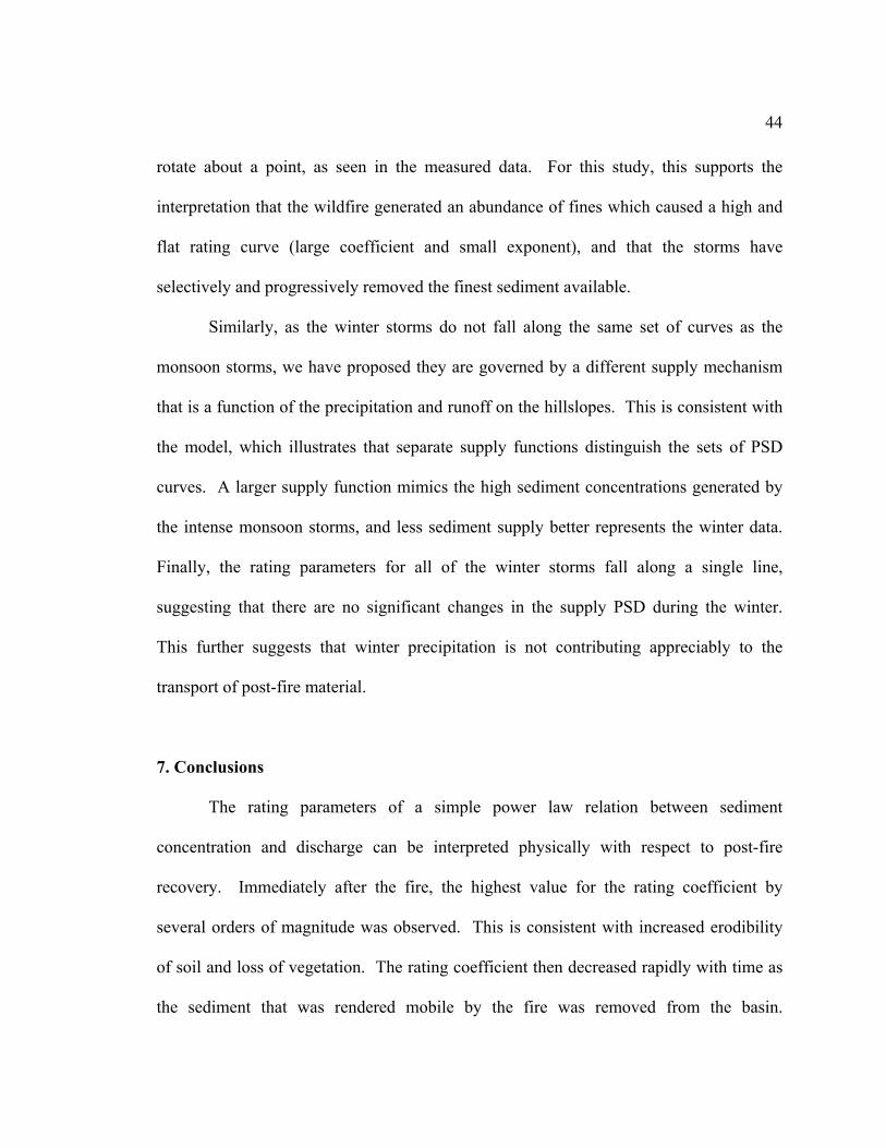
44

rotate about a point, as seen in the measured data. For this study, this supports the

interpretation that the wildfire generated an abundance of fines which caused a high and

flat rating curve (large coefficient and small exponent), and that the storms have

selectively and progressively removed the finest sediment available.

Similarly, as the winter storms do not fall along the same set of curves as the

monsoon storms, we have proposed they are governed by a different supply mechanism

that is a function of the precipitation and runoff on the hillslopes. This is consistent with

the model, which illustrates that separate supply functions distinguish the sets of PSD

curves. A larger supply function mimics the high sediment concentrations generated by

the intense monsoon storms, and less sediment supply better represents the winter data.

Finally, the rating parameters for all of the winter storms fall along a single line,

suggesting that there are no significant changes in the supply PSD during the winter.

This further suggests that winter precipitation is not contributing appreciably to the

transport of post-fire material.

7. Conclusions

The rating parameters of a simple power law relation between sediment

concentration and discharge can be interpreted physically with respect to post-fire

recovery. Immediately after the fire, the highest value for the rating coefficient by

several orders of magnitude was observed. This is consistent with increased erodibility

of soil and loss of vegetation. The rating coefficient then decreased rapidly with time as

the sediment that was rendered mobile by the fire was removed from the basin.

45

Following the fire, the rating exponent was low and then increased with time, indicating

the preferential removal of the smallest grain sizes.

The relationship between the rating coefficient and exponent showed a clear

distinction between the sediment transport regime during monsoon and winter storm

events. This was true even the first year following the fire. In particular, the rotation

pattern of the 2003 monsoon rating curves was disrupted by a distinct winter rating

relationship and then resumed during the 2004 monsoon. This seasonality is attributed to

processes that occur on the hillslopes rather than in the streambed: differences in

precipitation intensity and amount of overland flow between the monsoon and winter

seasons. Results from a numerical mass transport model support this interpretation. The

progression of the monsoon rating curves with time can be explained by changes in PSD

due to selective removal of fine particles. The winter rating curve behavior is consistent

with a distinct sediment supply function, based on hillslope processes, which does not

show effects of selective removal of fines.

Our study demonstrates that a disturbed ecosystem requires special consideration

when developing a sampling strategy. In the case of wildfire, increased soil erodibility

and sediment availability alter the previous pattern of sediment discharge. Therefore,

sampling must be designed to determine the hydrologically-forced periods of similar

sediment response and whether the system is changing within these periods. For the

Sabino watershed, high sampling frequency was redundant in the winter. However, for

the monsoon season, event-based sampling was necessary to determine the initial degree

of erosion damage and the rate of recovery. In particular, changes in the rating

46

parameters are shown to be a function of the number of intense rainstorms rather than of

time. These short-term dynamics have not been previously documented and can be

useful as constraints in rapid assessment fire-response models.

Acknowledgements

This work was funded by NSF Small Grants for Exploratory Research, EAR-

0342831, the Arizona University System Technology and Research Initiative Fund, TRIF

Grant P04-21, and the NSF Science and Technology Center for Semi-arid Hydrology and

Riparian Areas (SAHRA). The authors thank Maite Guardiola-Claramonte for assistance

with site maps, watershed variables and lab and field work, Karletta Chief for help with

sampling and lab work, and Evan Canfield of the Pima County Flood Control District and

an anonymous reviewer for constructive comments. We would also like to acknowledge

the support of the Coronado National Forest and the Fenster School for granting access to

field sites.

47

References

Agee, J.K., 1993. Fire ecology of Pacific Northwest Forests. Island Press, Washington D.C., 493 pp.

Adams, D.K. and Comrie, A.C., 1997. The North American Monsoon. Bulletin of the American Meteorological Society, 78(10): 2197-2213.

Anderson, H.W., Hoover, M.D. and Reinhart, K.G., 1976. Forests and water: effects of forest management on floods, sedimentation, and water supply. PSW-18, USDA, Forest Service, Berkeley, CA.

Asselman, N.E.M., 2000. Fitting and interpretation of sediment rating curves. Journal of Hydrology, 234(3-4): 228-248.

Campbell, R.E., Baker, M.B., Ffolliott, P.F., Larson, F.R. and Avery, C.C., 1977. Wildfire effects on a ponderosa pine ecosystem: an Arizona case study. RM-191, USDA Forest Service.

Cannon, S.H., Bigio, E.R. and Mine, E., 2001. A process for fire-related debris flow initiation, Cerro Grande fire, New Mexico. Hydrological Processes, 15(15): 3011-3023.

Cohn, T.A., 1995. Recent Advances in Statistical-Methods for the Estimation of Sediment and Nutrient Transport in Rivers. Reviews of Geophysics, 33: 1117-1123.

Cunningham, E.E.B., Long, A., Eastoe, C. and Bassett, R.L., 1998. Migration of recharge waters downgradient from the Santa Catalina Mountains into the Tucson basin aquifer, Arizona, USA. Hydrogeology Journal, 6(1): 94-103.

DeBano, L.F., 2000. The role of fire and soil heating on water repellency in wildland environments: a review. Journal of Hydrology, 231: 195-206.

DeBano, L.F., Neary, D.G. and Ffolliott, P.F., 1998. Fire's effects on ecosystems. John Wiley & Sons, New York ; Chichester [England], xvii, 333 pp.

DuBois, R.L., 1959. Petrography and structure of a part of the gneissic complex of the Santa Catalina Mountains, Arizona, AZ Geological Socity, Tucson, AZ.

Ewing, R., 1996. Postfire suspended sediment from Yellowstone National Park, Wyoming. Water Resources Bulletin, 32(3): 605-627.

Fisk, G.G. et al., 2004. Water Resources Data, Arizona, Water Year 2003. AZ-03-1, U.S. Geological Survey, Tucson, AZ.

48

Gabet, E.J., 2003. Post-fire thin debris flows: Sediment transport and numerical modelling. Earth Surface Processes and Landforms, 28(12): 1341-1348.

Goodrich, D.C. et al., 2005. Rapid post-fire hydrologic watershed assessment using the AGWA GIS-based hydrologic modeling tool., ASCE Watershed Management Conference, Williamsburg, VA, pp. 1-12.

Guardiola-Claramonte, M., 2005. Potential effects of wildfire on watershed hydrologic response: Sabino Creek Basin, Arizona. M.S. Thesis, University of Arizona, Tucson, AZ, 119 pp.

Hawkins, R.H., 2003. Survey of methods for sediment TMDLs in western rivers and streams of the United States. Grant #827666-01-0, US Environmental Protection Agency, Washington D.C.

Johnson, A., 2003. Aspen Fire 2003 Treatment success monitoring report, USDA Forest Service, Southwest Region.

Kurupakorn, S., 1973. Preliminary investigation of upper Sabino Canyon dam, Pima County, Arizona, 64 leaves. pp.

Lane, L.J., Foster, G.R. and Nicks, A.D., 1987. Use of fundamental erosion mechanics in erosion prediction. 87-2540, ASAE, St. Joseph, MI.

Lopes, V.L., Ffolliott, P.F. and Baker, M.B., 2001. Impacts of vegetative practices on suspended sediment from watersheds of Arizona. Journal of Water Resources Planning and Management-ASCE, 127(1): 41-47.

Miller, G. and Natharius, M., 2003. Assessment of soil resource conditions, Aspen Fire, USDA Forest Service, Tucson, AZ.

Moody, J.A. and Martin, D.A., 2001. Initial hydrologic and geomorphic response following a wildfire in the Colorado Front Range. Earth Surface Processes and Landforms, 26(10): 1049-1070.

Morehead, M.D., Syvitski, J.P., Hutton, E.W.H. and Peckham, S.D., 2003. Modeling the temporal variability in the flux of sediment from ungauged river basins. Global and Planetary Change, 39(1-2): 95-110.

Neary, D.G., Klopatek, C.C., DeBano, L.F. and Ffolliott, P.F., 1999. Fire effects on belowground sustainability: a review and synthesis. Forest Ecology and Management, 122(1-2): 51-71.

Nistor, C.J. and Church, M., 2004. Suspended sediment transport regime in a debris-flow gully on Vancouver Island, British Columbia. Hydrological Processes.

49

Norris, L.A., 1990. An overview and synthesis of knowledge concerning natural and prescribed fire in Pacific Northwest forests. In: J.D. Walstad, S.R. Radosevich and D.V. Sandberg (Editors), Natural and prescribed fire in Pacific Northwest forests. Oregon State University Press, Corvallis, Oregon, pp. 7-22.

Qian, N. and Wan, Z., 1999. Mechanics of sediment transport. American Society of Civil Engineers, Reston, Va., xix, 913 pp.

Rinne, J.N., 1996. Short-term effects of wildfire on fishes and aquatic macroinvertebrates in the southwestern United States. North American Journal of Fisheries Management, 16:653-658.

Robichaud, P.R., Beyers, J.L. and Neary, D.G., 2000. Evaluating the effectiveness of postfire rehabilitation treatments. RMRS-063, U.S. Department of Agriculture, Forest Service, Fort Collins, CO.

Syvitski, J.P., Morehead, M.D., Bahr, D.B. and Mulder, T., 2000. Estimating fluvial sediment transport: The rating parameters. Water Resources Research, 36(9): 2747-2760.

Thomas, R.B., 1988. Monitoring Baseline Suspended Sediment in Forested Basins - the Effects of Sampling on Suspended Sediment Rating Curves. Hydrological Sciences Journal-Journal Des Sciences Hydrologiques, 33(5): 499-514.

Veenhuis, J.E., 2002. Effects of wildfire on the hydrology of Capulin and Rito de los Frijoles Canyons, Bandelier National Monument, New Mexico. 02-4152, U.S. Geological Survey, Albuquerque, NM.

Walling, D.E., 1974. Suspended sediment and solute yields from a small catchment prior to urbanization. In: K.J. Gregory and D.E. Walling (Editors), Fluvial processes in instrumented watersheds : studies of small watersheds in the British Isles, Special publication - Institute of British Geographers ; no. 6. Institute of British Geographers, London (1 Kensington Gore, SW7 2AR), pp. iii, 196.

Walling, D.E., 1977. Assessing the accuracy of suspended sediment rating curves for a small basin. Water Resources Research, 13(3): 531-538.

Westerling, A.L. and Swetnam, T.W., 2003. Interannual to decadal drought and wildfire in the western United States. EOS Transactions AGU, 84(49): 545.

Williams, G.P. and Rosgen, D.L., 1989. Measured total sediment loads (suspended and bedload) for 93 United States streams. 89-67, U.S. Geological Survey.

50

Willis, I.C., Richards, K.S., and Sharp, M.J., 1996. Links between pro-glacial stream suspended sediment dynamics, glacier hydrology and glacier motion at Midtdalsbreen, Norway. Hydrological Processes, 10: 629-648.

51

List of Tables

Table 1. Sediment rating parameters from wildfire sediment studies in the Western U.S.

Table 2. Summary of sampled runoff events and rating parameters.

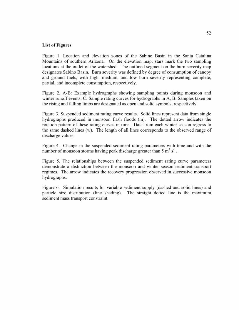
52

List of Figures

Figure 1. Location and elevation zones of the Sabino Basin in the Santa Catalina Mountains of southern Arizona. On the elevation map, stars mark the two sampling locations at the outlet of the watershed. The outlined segment on the burn severity map designates Sabino Basin. Burn severity was defined by degree of consumption of canopy and ground fuels, with high, medium, and low burn severity representing complete, partial, and incomplete consumption, respectively.

Figure 2. A-B: Example hydrographs showing sampling points during monsoon and winter runoff events. C: Sample rating curves for hydrographs in A, B. Samples taken on the rising and falling limbs are designated as open and solid symbols, respectively.

Figure 3. Suspended sediment rating curve results. Solid lines represent data from single hydrographs produced in monsoon flash floods (m). The dotted arrow indicates the rotation pattern of these rating curves in time. Data from each winter season regress to the same dashed lines (w). The length of all lines corresponds to the observed range of discharge values.

Figure 4. Change in the suspended sediment rating parameters with time and with the number of monsoon storms having peak discharge greater than 5 m3 s-1.

Figure 5. The relationships between the suspended sediment rating curve parameters demonstrate a distinction between the monsoon and winter season sediment transport regimes. The arrow indicates the recovery progression observed in successive monsoon hydrographs.

Figure 6. Simulation results for variable sediment supply (dashed and solid lines) and particle size distribution (line shading). The straight dotted line is the maximum sediment mass transport constraint.

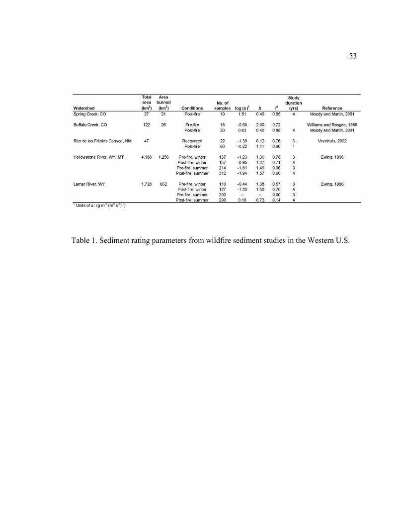
53

Table 1. Sediment rating parameters from wildfire sediment studies in the Western U.S.

54

Table 2. Summary of sampled runoff events and rating parameters.

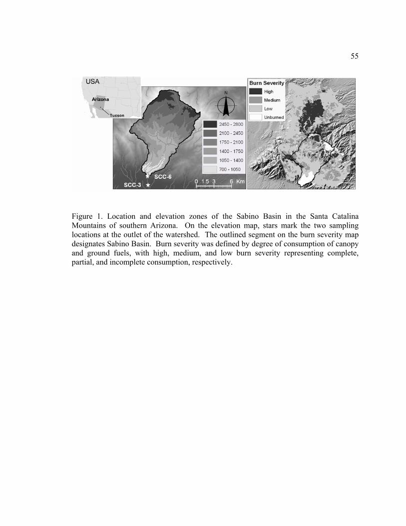
55

Figure 1. Location and elevation zones of the Sabino Basin in the Santa Catalina Mountains of southern Arizona. On the elevation map, stars mark the two sampling locations at the outlet of the watershed. The outlined segment on the burn severity map designates Sabino Basin. Burn severity was defined by degree of consumption of canopy and ground fuels, with high, medium, and low burn severity representing complete, partial, and incomplete consumption, respectively.

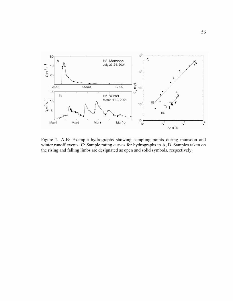
56

Figure 2. A-B: Example hydrographs showing sampling points during monsoon and winter runoff events. C: Sample rating curves for hydrographs in A, B. Samples taken on the rising and falling limbs are designated as open and solid symbols, respectively.

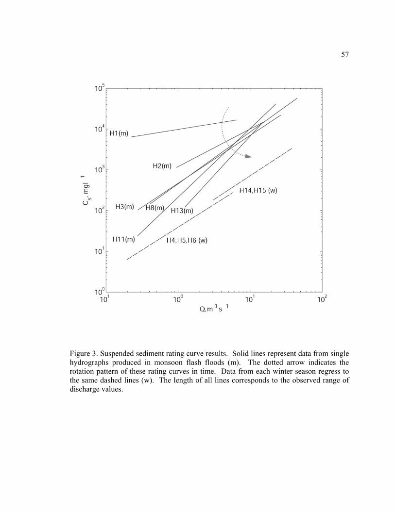
57

Figure 3. Suspended sediment rating curve results. Solid lines represent data from single hydrographs produced in monsoon flash floods (m). The dotted arrow indicates the rotation pattern of these rating curves in time. Data from each winter season regress to the same dashed lines (w). The length of all lines corresponds to the observed range of discharge values.

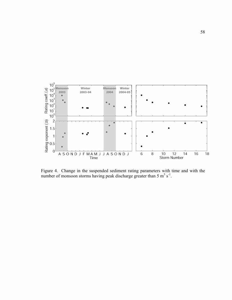
58

Figure 4. Change in the suspended sediment rating parameters with time and with the number of monsoon storms having peak discharge greater than 5 m3 s-1.

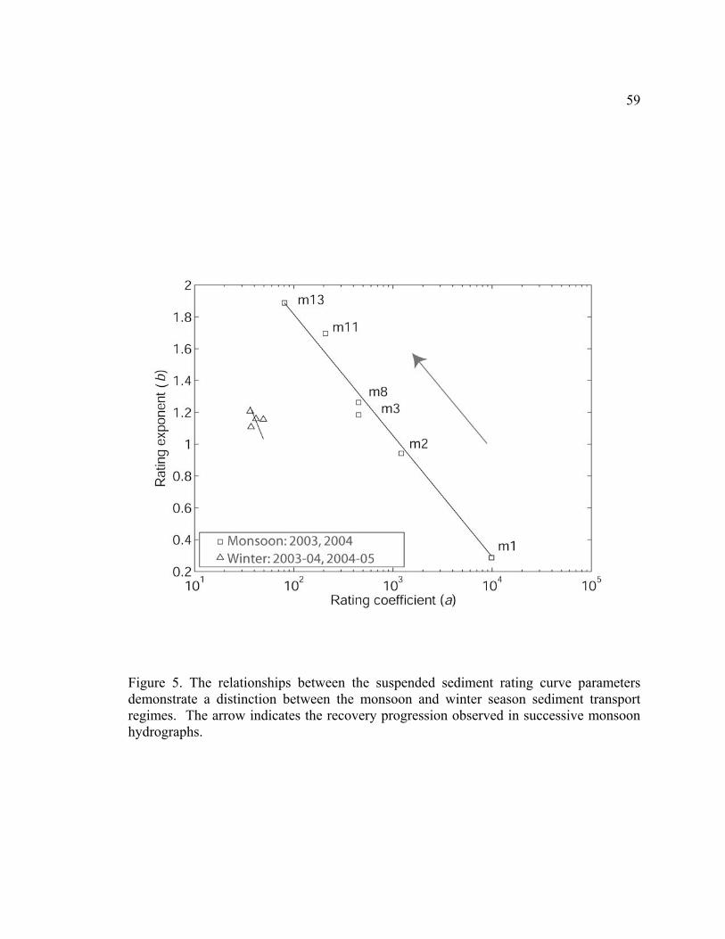
59

Figure 5. The relationships between the suspended sediment rating curve parameters demonstrate a distinction between the monsoon and winter season sediment transport regimes. The arrow indicates the recovery progression observed in successive monsoon hydrographs.

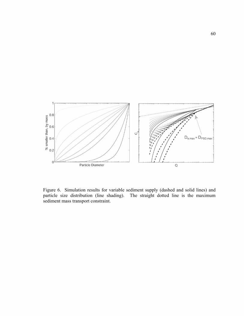
60

Figure 6. Simulation results for variable sediment supply (dashed and solid lines) and particle size distribution (line shading). The straight dotted line is the maximum sediment mass transport constraint.

61

APPENDIX B

FLASH FLOOD COMPOSITION IN A SEMI-ARID MOUNTAIN WATERSHED

Sharon L. E. Desilets1, Ty P. A. Ferré1, and Brenda Ekwurzel1,2

1 Department of Hydrology and Water Resources, University of Arizona, Tucson, Arizona, USA.

2 Present address: Union of Concerned Scientists, Washington D.C., USA

62

Abstract

Flash flood hydrographs were examined using water stable isotopes (deuterium and

oxygen) to assess the origin and routing of flood water in a semi-arid basin in the

southwestern United States. Precipitation and stream water were sampled during storm

and flood conditions at high and low elevations. Isotope mixing relationships readily

determined the predominance of three sources for the representative summer monsoon

events: high elevation precipitation from two major sub-basins, and baseflow. Each flood

progressed through a series of source water contributions as indicated by several

segments of linear mixing between these endmembers. We developed a plug-flow

lumped-catchment model to test possible governing processes for specific watershed and

forcing conditions. Results suggest two main findings. First, these flood events were

generated primarily from event water runoff in high elevations that mixed at the flood

bore with pre-event baseflow resident in the stream. The power, speed, and turbulence of

the flood bore cause it to mix with, ride atop, and push the resident in-stream water in the

front of the rising limb. Second, the timing and volume of flood waves from sub-basins

are identified by their combined isotopic signature at the basin outlet; this approach may

provide an effective mesoscale constraint for rainfall-runoff models.

63

1. Introduction

Flash floods are hazardous, short-lived, and difficult to predict. For these reasons,

data on their composition and dynamics are sparse and challenging to obtain even with

automated methods. They can be generated by high intensity rainfall, slow-moving storm

systems, and even rapid snowmelt (Merz and Bloschl, 2003). The danger associated with

these natural occurrences can be magnified by anthropogenic activities. In particular,

land-use change has increased the potential for damaging floods by deforesting and

urbanizing large areas of prior flood-mitigating vegetation (Larsen et al., 2001). Flash

floods cause significant damage worldwide and their financial toll grows annually due to

increasing population and infrastructure costs in close proximity to flood-prone areas

(Gruntfest and Handmer, 2001; Pielke et al., 2002). Further, they play an important role

in the long-term geomorphology, hydrology, and ecology of streams and rivers (Baker et

al., 1988).

Several approaches have been employed for flood modeling, as recently reviewed

by Beven (2005). The appropriate degree of complexity for a particular model

application depends on the scale of interest and information available (Sivapalan et al.,

2003). Downward modeling, an approach that focuses on the holistic behavior of a

system, has gained popularity for examining appropriate complexity and for identifying

the dominant modes of response to a system (Sivapalan and Young, 2005). This

approach offers promise for identifying the main hydrological processes important in

different climates, landscapes, and scales which could then be applied in models for

ungaged basins (Sivapalan et al., 2003).

64

Isotope hydrograph separations (IHS) have also been used to illuminate

hydrograph generation processes for several decades and the results in the literature can

be summarized for several representative climate and hydrological conditions. In high-

rainfall, response-dominated catchments, that have high quickflow/precipitation ratios,

the tendency to observe large volumes of pre-event water in the hydrograph depends

strongly on the precipitation intensity, which affects the degree of saturation overland

flow (Bonell et al., 1999). For example, steep, humid catchments studied in northeast

Queensland, with 10-minute maximum rainfall intensities (I10) near 80 mm h-1, showed a

dominance of event water in the hydrographs, with hydrometric data supporting

saturation overland flow as the dominant mechanism (Bonell et al., 1999). In contrast, in

the shallow-soil, steep slopes of the Maimai catchment in New Zealand, with 99% of

rainfall intensities < 9 mm h-1, McDonnell (1989) demonstrated the importance of

macropore flow for delivering a large volume of pre-event water to hydrograph peaks

through old water displacement. In the snow-melt dominated spring floods of the

Rockies and Sierra Nevada Ranges in the Western USA, several researchers have shown

the significant contribution from ‘old’ water (Huth et al., 2004; Liu et al., 2004;

Rademacher et al., 2005). These examples are in contrast to monsoonal flash floods in

low-elevation, low-relief semi-arid ephemeral washes that are entirely event water

(Ingraham et al., 1999). A less-explored category in this research is semi-arid

mountainous locations that combine conditions from these different groupings. These

areas include well-wetted humid-like conditions in the high elevations that transition to

ephemeral streams in the lower elevations, soil depths ranging from areas of considerable

65

storage capacity (several meters deep) to dominantly rock outcrops, and high-intensity

storms that can generate flash floods in the lower elevations. In addition to climate, study

scale will also dictate which hydrological processes dominate the stream composition.

The majority of IHS studies are done at a scale < 10 km2 (Bonnell, 2005) where hillslope

processes are observable, as opposed to larger scales where rapid transport in the channel

network dominates.

The Santa Catalina Mountains of southern Arizona provide an opportunity to

explore the main processes involved in flood generation and routing at the mesoscale (~

100 km2) in a semi-arid mountainous region. A conceptual model for flow contributions

and pathways was developed based on preliminary findings from field observations. For

this basin, the majority of rain events sampled for this study fell at high elevations where

the soils are thin and underlain by largely impermeable block granite and gneiss. Rilling

and overland flow are visible at high elevations during rain events, and flash floods result

with sharp rising limbs (baseflow to peak conditions quicker than the 15 minute

resolution of the stream gage). Our conceptual model proposes that, for these types of

events in this basin, overland flow dominates the stream water composition at high

elevation and generates flood waves, and that these waves compress and mix with

resident stream baseflow as they coalesce and move down the canyon. To test this, the

objectives of this paper are (1) to use isotopes to identify the relative source water

contributions to a flash flood, (2) to develop a simple plug-flow lumped-catchment model

and apply it to data from two example storm events, and (3) to demonstrate how this

information can indicate the timing of flood contributions from individual canyons in the

66

studied basin and (4) explore flood bore dynamics. Finally, we consider how information

obtained from this isotopic approach to studying flash floods could be further explored

for application in downward modeling.

2. Site Description

The Sabino Creek watershed, located northeast of Tucson, Arizona, is on the

south-facing slope of the Santa Catalina Mountains (Figure 1). This range is part of a

northwest trending series of metamorphic blocks in the southeast portion of the Basin and

Range region. The bedrock is predominantly granite and gneiss, with steep and rugged

terrain covered by thin soils, ranging from less than 0.25 m to more than 1.5 m deep

(DuBois, 1959; Whittaker et al., 1968). The total area of the watershed is 91 km2 with

elevations ranging from 823 m at the base of the mountains to 2,789 m at the summit of

Mt. Lemmon, the highest peak in the range. Sabino Creek is the main ephemeral stream

in the watershed, registering flow at the gage an average of 294 days per year with a

mean flow of 0.41 m3 s-1 at the outlet of the basin (LSC1, Figure 1) (Guardiola-

Claramonte, 2005; USGS Stream Gage ID#94840010). The watershed comprises two

major sub-basins in its higher elevations, the Upper Sabino Creek and the Palisade Creek

sub-basins, with areas of 45.1 and 22.2 km2, respectively. The highest peaks in each of

these are Mt. Lemmon, elevation 2789 m, and Mt. Bigelow, elevation 2606 m,

respectively. The confluence of the Sabino and Palisade creeks is at an elevation of 1100

m (near MSC1 in Figure 1) ; after this point there is only one other significant tributary,

Rattlesnake Canyon, before the outlet of the watershed (near LSC1 in Figure 1).

67

The watershed is located near the eastern limit of the Sonoran desert, within a

semi-arid climate. The vegetation varies from southwestern desert shrub at low

elevations, to broadleaf woodland chaparral between 1300 and 2200 m, and mixed-

coniferous forest at the highest elevations (Whittaker and Niering, 1965). The average

annual precipitation is 0.3 m at the base and 0.8 m near the summit (Guardiola-

Claramonte, 2005). The precipitation falls predominantly during two distinct seasons: a

summer monsoon season (usually July through September) and a winter season (with the

majority of precipitation occurring between December and March), separated by typically

dry periods.

Southern Arizona lies within the influence of the North American Monsoon

(Adams and Comrie, 1997). It is characterized by localized afternoon convective storms

of high rainfall intensity and short duration. For our study site and study period, the

average duration is usually a few hours and the average I10 is 73 mm h-1 (Desilets, 2007).

This produces a sharply peaked flash flood; flow returns to less than 1 m3 s-1 within a

couple of days. The flow has been observed to dry completely when there are several

weeks between storms. Winter precipitation in Sabino Creek watershed often are Pacific

ocean frontal storms that are longer duration (a few days) and have lower rainfall

intensity (average I10 = 13 mm h-1 (Desilets, 2007)). These frequently result in snow at

high elevations, much of which, during the study period, melted within days or weeks

after the storm passed.

68

3. Model Description

Based on field observations and the hydrogeology of the basin, flood formation is

hypothesized to develop from predominantly event water runoff that mixes dispersively

at the flood bore with resident stream water. The following is a simple formalization of

these processes in a lumped-catchment plug-flow mixing model. It is designed for a

semi-arid basin with a few major sub-basins. The model is intentionally minimal in its

input requirements to be applicable to basins without extensive hydrometric data

available; instead, geochemistry is employed as an integrating parameter to discern the

first order controls on flood water composition.

Figure 2 show a diagram to summarize the main components of the model. In its

essence, the model is a linear mixing of flow and chemistry in two or more stream

hydrographs below the confluence of the streams. The water balance is established by

the hydrographs above the confluence if available, or can be approximated by a

lognormal distribution as described below. The chemistry in each hydrograph is defined

based on the hypothesis of plug flow in the stream channel with mixing at the front of the

flood wave. At this interface there is mixing between two isotopically distinct waters: (1)

flood water, assumed to be event water, and (2) the resident pre-event baseflow in the

channel. The advection-dispersion equation is used to describe the step pulse change

from one endmember concentration to the other and back again.

If a flow gage at the point of interest, just upstream of the confluence, is not

available, a hydrograph shape can be represented as a normalized lognormal distribution

69

2

2

2))(ln(

21)( σ

µ

πσ

−−

=t

et

ty (1)

where y(t) is the height of the volumetric flow hydrograph and t is time. The mean (µ)

and standard deviation (σ) are adjusted to match the shape of other available hydrographs

in the respective sub-basins. The peaks of the generalized hydrographs are scaled to

match relative volumes of precipitation in each sub-basin for a given event so that the

volumetric flow rate (Q) is defined as

max)()()(

tytyftQ ii = (2)

where f is the fraction of total rain volume and i denotes an individual sub-basin.

The isotope chemistry of the water in each sub-basin hydrograph is calculated as a

plug flow of event water with mixing between event and pre-event water at the front and

tail end of the hydrograph as given by the advection-dispersion equation (ADE) (Ogata

and Banks, 1961),

xCv

xCD

tC

xL ∂∂

−∂∂

=∂∂

2

2

(3)

where C is the isotope concentration, DL the coefficient of longitudinal hydrodynamic

dispersion, vx is the average velocity in the x-direction, defined by the celerity of the

70

flood wave, and t is the time of input of a particular isotope concentration. The solution

for a continuous injection is

( ) ( ) ( )

+

−

−

= R

R

eeR

R

eR t

tPerfcPt

tPerfcC 1

4exp1

45.0

21

21

(4)

where the dimensionless forms of concentration and time are defined as

maxCCCR = (5)

Ltv

t xR = (6)

and the Peclet number (Pe) as

L

xe D

LvP = . (7)

Isotope concentrations are varying between two endmembers for each sub-basin: (1)

event water as determined from rain sampling and (2) resident baseflow as determined

71

from stream sampling. The relative concentration (CR) represents the fraction of water

with the breakthrough endmember.

This ADE solution is applied at two points in the hydrograph: (1) at the flood bore

where it interfaces between flood event water and pre-event baseflow and (2) at the point

in the recession where the event water begins to be replaced by baseflow, isotopically.

),(),( ,, reRRfeRi PttfPtfC ∆+−= (8)

where ∆tR represents the time between the initial transition to event water and the later

transition back to baseflow, and the Peclet numbers are specified for the flood rising limb

(Pe,f) and recession (Pe,r). The Peclet numbers vary because of the two different

velocities occurring at two these stages of the hydrograph. Additive mixing of the water

from each channel determine the water volume and chemistry below the confluence of

the sub-basin streams according to

∑=

=n

iitotal tQtQ

1)()( (9)

∑

∑

=

== n

ii

n

iii

mix

tQ

tQtCtC

1

1

)(

)()()( (10)

72

where n is the total number of sub-basins considered and C(t)mix is the resultant isotopic

concentration.

Ideally, the minimum known parameters for application of the model are the

isotopic value of the precipitation endmember, hydrograph shape, flood wave celerity,

and stream length for each of the individual sub-basins. The adjustable parameters for

fitting the model results to stream isotopic data are the dispersion coefficient and time

between the initial transition to event water and the later transition back to baseflow.

4. Method

To test our conceptual model and characterize the response of the system to

monsoon storms, precipitation and stream water samples were collected throughout

selected events. In the streams, grab samples were collected in glass bottles with

Polyseal® caps. The main sampling site was along the Lower Sabino Creek (LSC1)

(Figure 1) at the base of the watershed (elevation 829 m) at a United States Geological

Survey flow gage (ID #94840010). This gage resides at Sabino Dam, a reservoir built in

the 1930s, which has since filled with sediment (Kurupakorn, 1973). This feature

minimizes scour-fill challenges typical of other gaging stations on alluvial channels. The

gage measures stream height with a pressure transducer every fifteen minutes with 0.3 cm

precision. Due to the flashy nature of most monsoon flood events during the study

period, the gage often jumped from a zero value (i.e. if there was flow it was below

minimum gage measurement level) to the maximum registered flow for the hydrograph

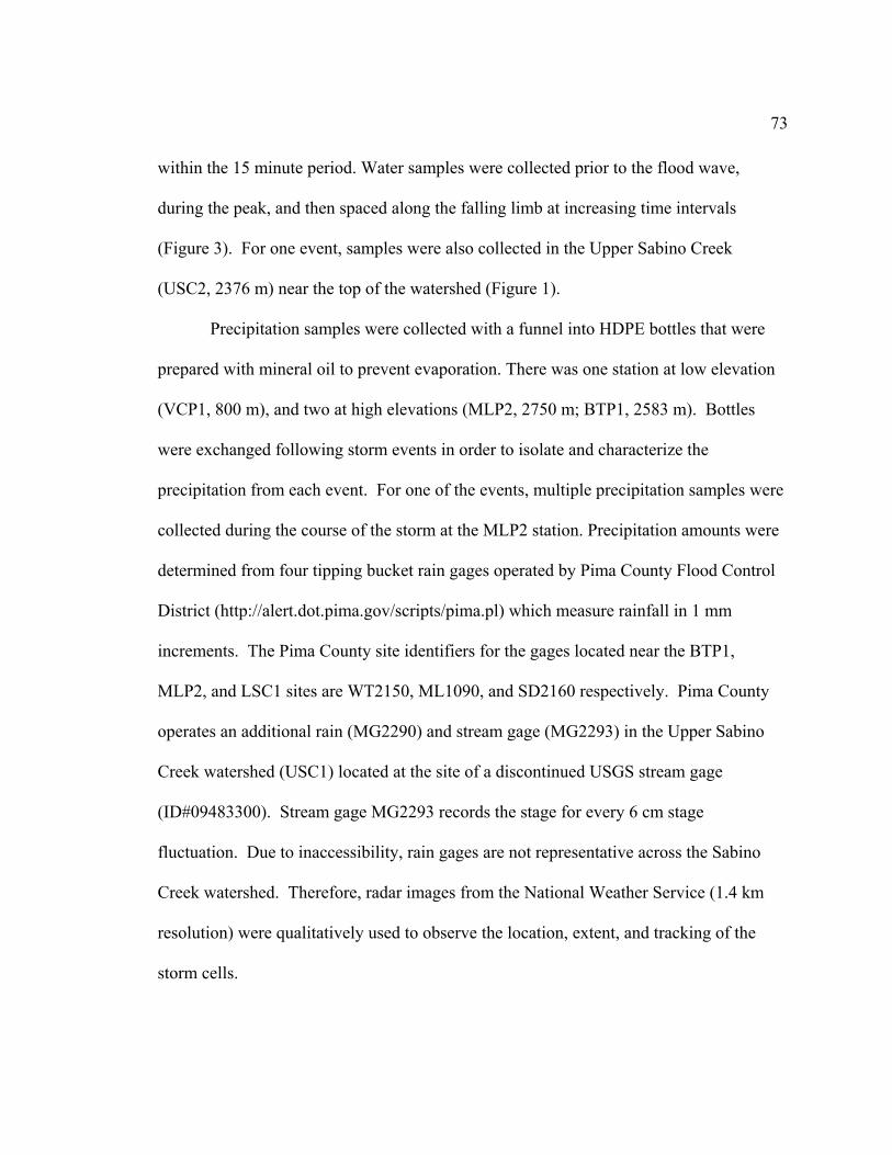
73

within the 15 minute period. Water samples were collected prior to the flood wave,

during the peak, and then spaced along the falling limb at increasing time intervals

(Figure 3). For one event, samples were also collected in the Upper Sabino Creek

(USC2, 2376 m) near the top of the watershed (Figure 1).

Precipitation samples were collected with a funnel into HDPE bottles that were

prepared with mineral oil to prevent evaporation. There was one station at low elevation

(VCP1, 800 m), and two at high elevations (MLP2, 2750 m; BTP1, 2583 m). Bottles

were exchanged following storm events in order to isolate and characterize the

precipitation from each event. For one of the events, multiple precipitation samples were

collected during the course of the storm at the MLP2 station. Precipitation amounts were

determined from four tipping bucket rain gages operated by Pima County Flood Control

District (http://alert.dot.pima.gov/scripts/pima.pl) which measure rainfall in 1 mm

increments. The Pima County site identifiers for the gages located near the BTP1,

MLP2, and LSC1 sites are WT2150, ML1090, and SD2160 respectively. Pima County

operates an additional rain (MG2290) and stream gage (MG2293) in the Upper Sabino

Creek watershed (USC1) located at the site of a discontinued USGS stream gage

(ID#09483300). Stream gage MG2293 records the stage for every 6 cm stage

fluctuation. Due to inaccessibility, rain gages are not representative across the Sabino

Creek watershed. Therefore, radar images from the National Weather Service (1.4 km

resolution) were qualitatively used to observe the location, extent, and tracking of the

storm cells.

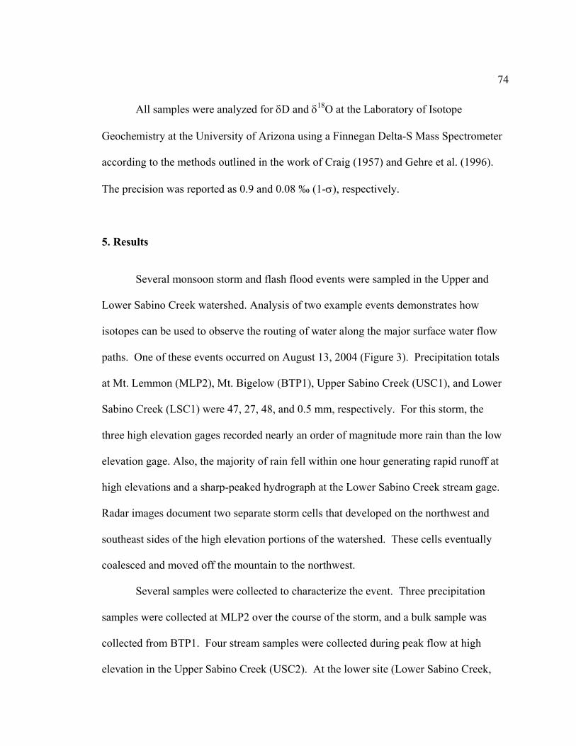
74

All samples were analyzed for δD and δ18O at the Laboratory of Isotope

Geochemistry at the University of Arizona using a Finnegan Delta-S Mass Spectrometer

according to the methods outlined in the work of Craig (1957) and Gehre et al. (1996).

The precision was reported as 0.9 and 0.08 ‰ (1-σ), respectively.

5. Results

Several monsoon storm and flash flood events were sampled in the Upper and

Lower Sabino Creek watershed. Analysis of two example events demonstrates how

isotopes can be used to observe the routing of water along the major surface water flow

paths. One of these events occurred on August 13, 2004 (Figure 3). Precipitation totals

at Mt. Lemmon (MLP2), Mt. Bigelow (BTP1), Upper Sabino Creek (USC1), and Lower

Sabino Creek (LSC1) were 47, 27, 48, and 0.5 mm, respectively. For this storm, the

three high elevation gages recorded nearly an order of magnitude more rain than the low

elevation gage. Also, the majority of rain fell within one hour generating rapid runoff at

high elevations and a sharp-peaked hydrograph at the Lower Sabino Creek stream gage.

Radar images document two separate storm cells that developed on the northwest and

southeast sides of the high elevation portions of the watershed. These cells eventually

coalesced and moved off the mountain to the northwest.

Several samples were collected to characterize the event. Three precipitation

samples were collected at MLP2 over the course of the storm, and a bulk sample was

collected from BTP1. Four stream samples were collected during peak flow at high

elevation in the Upper Sabino Creek (USC2). At the lower site (Lower Sabino Creek,

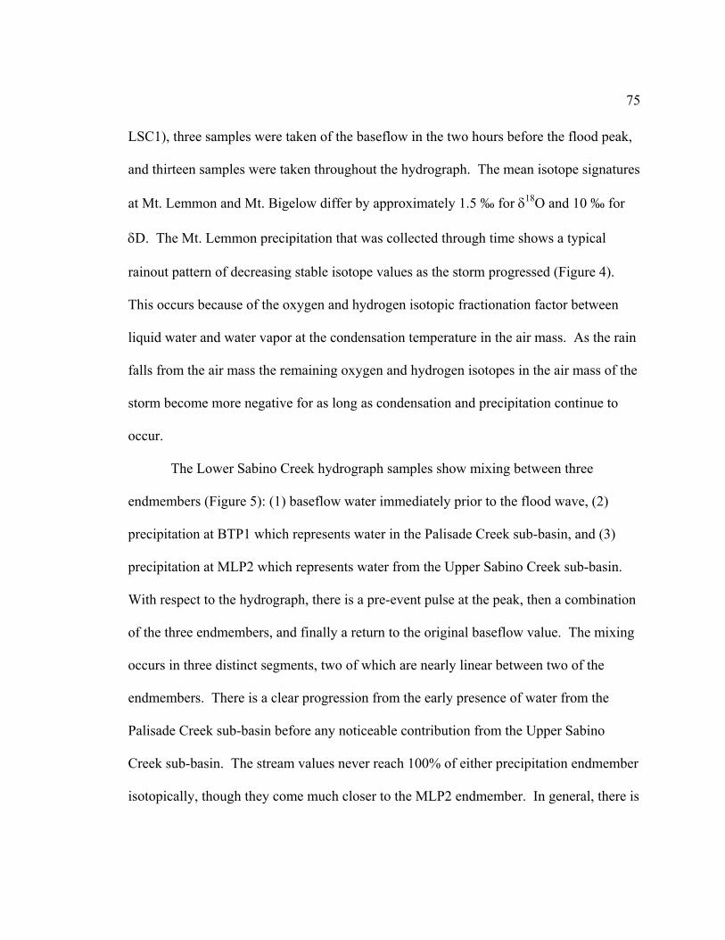
75

LSC1), three samples were taken of the baseflow in the two hours before the flood peak,

and thirteen samples were taken throughout the hydrograph. The mean isotope signatures

at Mt. Lemmon and Mt. Bigelow differ by approximately 1.5 ‰ for δ18O and 10 ‰ for

δD. The Mt. Lemmon precipitation that was collected through time shows a typical

rainout pattern of decreasing stable isotope values as the storm progressed (Figure 4).

This occurs because of the oxygen and hydrogen isotopic fractionation factor between

liquid water and water vapor at the condensation temperature in the air mass. As the rain

falls from the air mass the remaining oxygen and hydrogen isotopes in the air mass of the

storm become more negative for as long as condensation and precipitation continue to

occur.

The Lower Sabino Creek hydrograph samples show mixing between three

endmembers (Figure 5): (1) baseflow water immediately prior to the flood wave, (2)

precipitation at BTP1 which represents water in the Palisade Creek sub-basin, and (3)

precipitation at MLP2 which represents water from the Upper Sabino Creek sub-basin.

With respect to the hydrograph, there is a pre-event pulse at the peak, then a combination

of the three endmembers, and finally a return to the original baseflow value. The mixing

occurs in three distinct segments, two of which are nearly linear between two of the

endmembers. There is a clear progression from the early presence of water from the

Palisade Creek sub-basin before any noticeable contribution from the Upper Sabino

Creek sub-basin. The stream values never reach 100% of either precipitation endmember

isotopically, though they come much closer to the MLP2 endmember. In general, there is

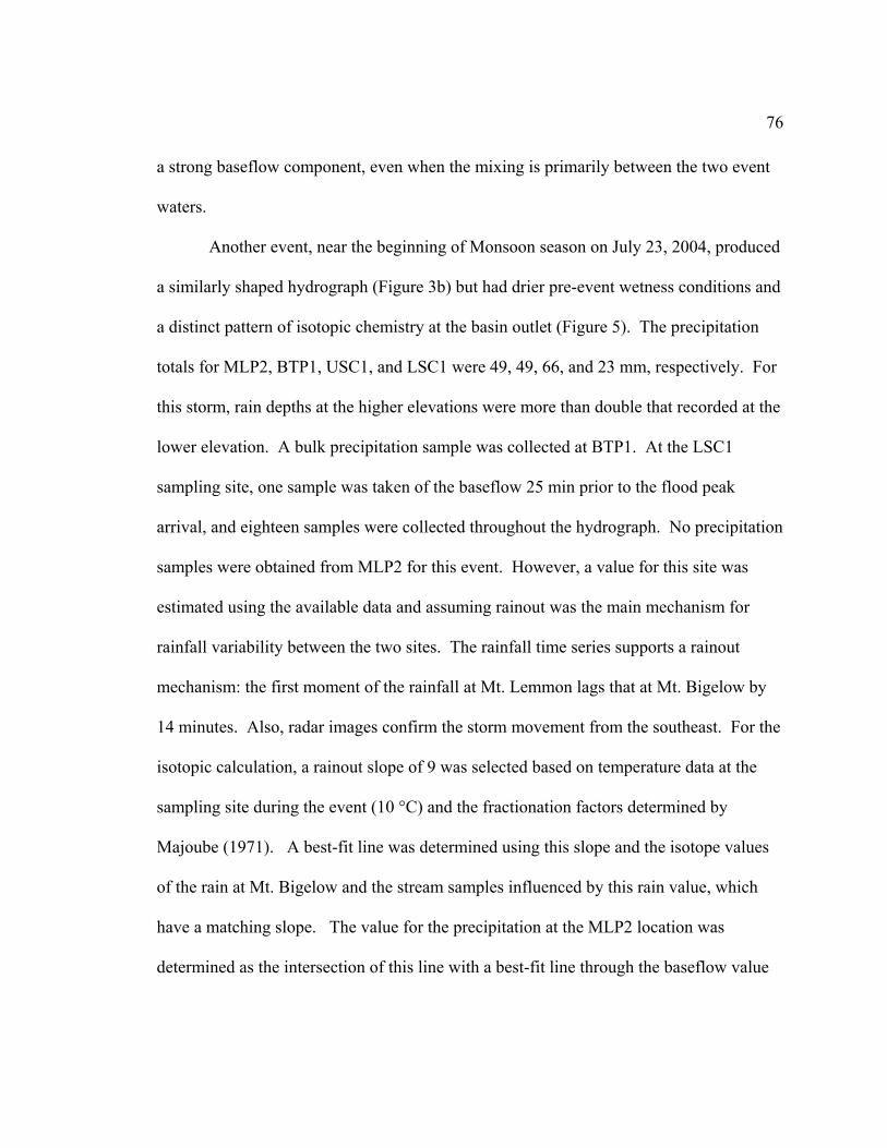
76

a strong baseflow component, even when the mixing is primarily between the two event

waters.

Another event, near the beginning of Monsoon season on July 23, 2004, produced

a similarly shaped hydrograph (Figure 3b) but had drier pre-event wetness conditions and

a distinct pattern of isotopic chemistry at the basin outlet (Figure 5). The precipitation

totals for MLP2, BTP1, USC1, and LSC1 were 49, 49, 66, and 23 mm, respectively. For

this storm, rain depths at the higher elevations were more than double that recorded at the

lower elevation. A bulk precipitation sample was collected at BTP1. At the LSC1

sampling site, one sample was taken of the baseflow 25 min prior to the flood peak

arrival, and eighteen samples were collected throughout the hydrograph. No precipitation

samples were obtained from MLP2 for this event. However, a value for this site was

estimated using the available data and assuming rainout was the main mechanism for

rainfall variability between the two sites. The rainfall time series supports a rainout

mechanism: the first moment of the rainfall at Mt. Lemmon lags that at Mt. Bigelow by

14 minutes. Also, radar images confirm the storm movement from the southeast. For the

isotopic calculation, a rainout slope of 9 was selected based on temperature data at the

sampling site during the event (10 °C) and the fractionation factors determined by

Majoube (1971). A best-fit line was determined using this slope and the isotope values

of the rain at Mt. Bigelow and the stream samples influenced by this rain value, which

have a matching slope. The value for the precipitation at the MLP2 location was

determined as the intersection of this line with a best-fit line through the baseflow value

77

and the stream samples influenced by the mixing between the baseflow and storm water

(Figure 5). The estimated value for MLP2 is (δD, δ18O) = (-53, -8 ‰).

As in the previous event, the isotope values in the Lower Sabino Creek samples

show nearly linear mixing between three endmembers; however, the shape of the mixing

lines differ significantly (Figure 5). This dissimilarity indicates a divergence in the order

of the flood water contributions from the endmember sub-basins. The pattern suggests

that water from the Upper Sabino Creek sub-basin arrives first, followed by a distinct

contribution from Palisade Creek sub-basin, after which the data retraces itself back to

Upper Sabino Creek water and finally back to pre-event water. Also, there is much less

contribution from baseflow throughout, and though the water eventually evolves toward

the pre-event conditions, it does not reach that value by the last sample collected three

days after flood peak.

6. Discussion

6.1 Model Application

The lumped-catchment plug-flow model is applied to this study area to test the

underlying hypotheses for processes contributing to flow in semi-arid catchments, with

the intent to characterize dominant processes that can be applied in other similar semi-

arid settings. The model structure reflects the geometry of Sabino Creek watershed with

two high elevation sub-basins (Upper Sabino Creek and Palisade Creek). The event

water endmember for each sub-basin is from the bulk samples collected at the MLP2 and

BTP1 sites. Although rain is distributed over the watershed, we assume the isotope

78

concentration that falls in a sub-basin is quickly organized into a well-mixed flood bore

with composition equal to the depth-averaged value observed in precipitation samples.

The baseflow endmember is taken as the average of isotope values from the samples

collected immediately before the arrival of the flood wave. Based on the catchment

geometry and the isotopic endmembers for a particular rain event, the model simulates

the isotopic composition of the flood water, which can be compared with the isotopic

composition of samples collected through time at LSC1.

The model in this form is applied to the two precipitation events described above,

with parameters of the advection dispersion equation calculated for the details of each

event. The average velocity (vx) is taken as the celerity of the flood wave as determined

from the travel time of the peak between the stream gage at high elevation and that at the

basin outlet (Figure 1), approximately 10 km h-1 for both events. Due to the limited

availability of flow data, this value is determined based on a gage in Upper Sabino Creek

and applied for both sub-basins. The length (L) of the stream for each sub-basin is from

the streams’ origins to their confluence, 15 and 8 km for the Upper Sabino Creek and

Palisade Creek sub-basins, respectively. The longitudinal dispersion is defined in general

terms as DL = σ2/2t where σ2 is the variance of the spreading. For Sabino Creek, we have

no a priori information on this value, and optimized it as a fitting parameter in the model

(equations 7, 8, and 10). From this, we determined values near 5 km2 h-1 for the rising

limb of our events, which yields a Peclet number (Pe = vxL/DL) of 30. This value is lower

than expected, indicating a large amount of dispersive spreading. We hypothesize that as

the flood bore advances it flows atop the slower moving baseflow more quickly than the

79

baseflow is incorporated by the turbulent front. This behavior has been observed during

field sampling. The second optimized parameter in our model was the time between the

initiation of the event and the initiation of return to baseflow (∆tr, equations 8 and 10).

This was determined from the timing of the transitions between the isotope event and

baseflow endmembers to be approximately 13 h for the events evaluated. The model is

designed to predict water chemistry beneath the confluence of the selected sub-basins.

Due to the inaccessibility of this point in the Sabino Creek watershed, flow data is

unavailable from this area and samples were collected farther downstream (LSC1). For

flow data, we fitted lognormal parameters (µ, σ) to hydrographs at USC1 and LSC1 and

used these as constraints for the modeled hydrographs above the confluence.

The two events considered were selected as instructive because the spatial

variability in the precipitation endmembers for the high elevation sub-basins (∆(δ18O,

δD) = 1.5, 10 ‰) allows for straightforward identification of the water at the basin outlet.

The variability is exploited by setting the average rain isotope value from each location as

an independent endmember to track the input signature of water in each respective sub-

basin. In support of this approach, we compared the high elevation precipitation at Mt.

Lemmon with the high elevation Upper Sabino Creek water and found the data match

closely (Figure 4). The similarity between the stream and rainfall isotope values suggests

a large and rapid influence of event water in the high elevation runoff. In this case, the

surface runoff from each sub-basin should be distinguishable and isotopically similar to

the precipitation, and may be used to estimate the timing and quantities of the

contributing source water to the hydrograph at the Lower Sabino Creek outlet.

80

The model captures the shape and progression of the isotope values at the basin

outlet for both events (Figure 6) in spite of differences between their precipitation

amounts, pre-event wetness conditions, endmember isotope values, and resultant outflow

isotope pattern. For the event on August 13, 2004, there is, first, linear mixing between

the pre-event baseflow and event water from the Palisade Creek sub-basin. This is

consistent with an interpretation of mixing between the resident stream water at the flood

bore with the overland and rapid through-flow of the Palisade Creek sub-basin event

water. When the second flood wave arrives from the Upper Sabino Creek sub-basin it

too is advancing a pre-event pulse, though it only includes water that was resident in the

higher elevation stream; the water initially present in the lower stream was already

displaced by the first flood wave. The isotope data moves along a curved path

representing the mixing of all three endmembers which progresses towards a dominance

of the event water from the Upper Sabino sub-basin. As the runoff recedes there is a

return to the original pre-event baseflow conditions. For the July 23 event, the model

pattern closely matches the measured isotope results where the Upper Sabino Creek sub-

basin water arrives first, followed by a distinct contribution from Palisade Creek sub-

basin, after which the data retraces itself back to Upper Sabino Creek water and finally

back to pre-event water. This supports the hypothesis that the flood bore mixes with

resident stream water and pushes it to the front of the hydrograph, a behavior also

observed by Nolan and Hill (1990). Further, it illustrates how the efficient combination

of isotope data combined with volume at a few locations in this type of watershed can be

a practical tool for water district managers.

81

These model results can be contrasted with what would be expected from

conceptual models that emphasize alternative endmembers or processes. Other possible

endmembers considered include low elevation precipitation, an elevation-averaged

precipitation value which is based on isotope elevation gradient from low and high

elevation samples, the previous event precipitation, high elevation baseflow, and the

previous event runoff. Each of these endmembers were individually considered in the

model for several events, but yielded a different pattern than that observed at the basin

outlet. In contrast, the high elevation and baseflow endmembers yielded a close

relationship between the modeled and hydrograph values for several storm events. For

example, low elevation precipitation and high elevation baseflow are significantly

enriched and depleted, respectively, compared to the initial baseflow values and the

pattern during the hydrograph peak and recession (see Figures 3 and 4).

Alternative processes for delivering pre-event water to the stream would also

yield a different isotopic pattern. In particular, if the majority of the pre-event water were

from groundwater storage, whether incorporated by rapid water table development and

macropore flow or by throughflow, that endmember would be isotopically lighter than

observed (Figure 4). This is because persistent baseflow from groundwater storage

occurs only at high elevations. Baseflow samples collected at high elevations (USC2) for

over three years shows that the isotope value for this water maintains a consistently

negative value near -65 ‰ δD, -9 ‰ δ18O (Figure 4). If this was rapidly transported to

the stream during a flood event we would expect to see a large contribution from this

endmember in the flood peak. In contrast, for the August 13 event, the isotope chemistry

82

of the peak flood water moves immediately from the pre-flood baseflow value toward the

isotopically heavier value of the Palisade Creek sub-basin, rather than in the negative

direction that would represent high elevation groundwater (Figures 3 and 4).

6.2 Pre-event water in mountainous semi-arid flash floods

Our formalized conceptual model has been shown to predict isotope values for

two different storm conditions in the watershed, but it includes strict assumptions about

the nature of the pre-event water. Namely, the model assumes that all of the pre-event

water was originally stored in the stream. Therefore, as a further test of these

assumptions, we verify whether there is sufficient storage in the stream to account for all

of the observed pre-event water by comparing the volume of pre-event water as

determined from isotope hydrograph separation (IHS) with a volume estimate of

baseflow resident in the stream based on stream length and gage height dimensions. Our

former analysis has been independent of IHS, and its introduction here requires a brief

statement of caution. Past researchers have shown that the commonly made assumptions

of constant spatial and temporal endmembers can be invalid in small basins (Buttle,

2005). In the case of the two storm events studied, we do observe spatial and temporal

variability. At the basin-scale there appears to be adequate averaging of event water in

the channel network to allow for the identification of a few dominant endmembers;

however, the variability is expected to introduce some error into the volume calculations

which is difficult to quantify without higher resolution sampling. Therefore, the volumes

83

presented are estimates calculated for the exercise of comparing order of magnitude

quantities.

For the August 13 event, the volume of pre-event water between points 1 and 2

(Figure 5) was calculated to be 11,500 m3 using IHS. Assuming the conditions of our

conceptual model, this volume is attributed to the water in the streams in Palisade Creek

sub-basin all the way to the larger basin outlet. Similarly, for the hydrograph segment

between 2 and 3 (Figure 5), the volume determined from IHS is 19,500 m3. This

represents water in the streams of the Upper Sabino Creek sub-basin. The total volume,

31,000 m3, yields an equivalent cross sectional area of 0.4 m2 water surface all the way

along the channel. For comparison with these values, the volume of water resident in the

stream prior to the flood event was estimated. To do this, gage height data collected

immediately prior to the flood wave were used from three locations (Figure 1): Upper

Sabino Creek (USC1), confluence of the Sabino and Palisade streams (MSC1), and

Lower Sabino Creek (LSC1). For the confluence location, the gage was not available

until after the studied storm events, so data from a similar event were used. The value for

the cross sectional area used for the upper and lower stream lengths was the average of

the confluence and high elevation, and confluence and low elevation gages, respectively.

This approach yielded a volume of water residing in the combined Palisade and Lower

Sabino Creek sub-basins, which represents the hydrograph segment from 1 to 2 (Figure

5), of 18,000 m3. For the Upper Sabino Creek sub-basin (represented by the segment

between points 2 to 3, Figure 5) the volume was 10,500 m3. These values can be

considered a conservative estimate in that they do not consider water stored in the

84

abundant pools found in the basin. Based on these estimates, the total resident stream

water from both approaches is approximately 30,000 m3. The similarity of this result

from independent methods provides additional support for our hypothesis that resident

stream water is an important component of a flash flood peak and influences flood bore

dynamics.

Based on the model results and above analysis we propose that, when delineating

water sources for flash floods at the basin scale, a source of water must be considered that

may not be significant for less flashy hydrographs: the resident in-stream water. The

relative importance of this pre-event source likely reflects the rapid timescales (on the

order of hours) involved. For Sabino Creek watershed, the time between peak rain and

peak runoff at high elevation (for an 8 km2 catchment) can be as short as 25 min and the

same peak arrives at the basin outlet in less than 2 h (July 23 event). The turbulent flood

bore readily incorporates the resident stream water so that what would have taken days to

travel from top to bottom under baseflow conditions now does so along with the rest of

the flood in hours, thus compressing its timing and making it a significant component of

the peak. In addition, basin size likely plays an important role in the observed results.

Although a consistent relationship has not been developed between basin scale and event

water (Bonnell, 2005), our results suggest the importance of the flood bore for producing

a pre-event component in the flood peak. At the ~ 100 km2 scale, the flood bore has time

to develop and advance atop and mix with the resident stream water; this process would

not be expected at the hillslope scale. Several mechanisms have been identified in the

literature for delivering pre-event water to a flood wave (e.g. Jones et al., 2006;

85

McDonnell, 1990). All of these contributors likely play some role in most systems, but

the dominant source varies by climate, hydrogeology, and basin size. For mountainous

semi-arid regions with intense storm forcing inputs, resident stream water is the main

component of the pre-event water in the hydrograph.

6.3 Application to Downward Modeling of Basin-Scale Runoff Processes

The scale of the data collected in this study is well suited for a downward

modeling approach that emphasizes the larger basin-scale outcomes over the summation

of the microscale, as advocated by Sivapalan and Young (2005). There are a few main

differences between the two examined storm events that illuminate the type of basin-scale

information from this analysis that would be useful in runoff and flood routing models.

Three examples are briefly explored below: soil wetness, bank storage, and flood peak

timing.

The July 23 event was the first major flood of the season, with dry pre-event soil

conditions. In contrast, the week prior to the August 13 event there had been several days

of low intensity rain. Repeated rain events and antecedent moisture conditions have been

shown to affect the relative importance of different runoff generating mechanisms in

semi-arid watersheds (Dick et al., 1997; Lange et al., 2003). In our data, this manifested

itself as a difference in the volume of pre-event water, with the lower volume of baseflow

in the stream under drier conditions: the July 23 event had much less pre-event water in

both the initial peak and in the peak for the flood wave from the second sub-basin.

Because the pre-event water is an important component of the flood peak at the basin

86

outlet, this information is critical for predicting peak height. In particular, if several

floods were examined in combination with measured soil conditions, a general basin-

scale relationship could be established to predict the percentage of event water and the

relative contributions of pre-event and storm water runoff, with the aim of quantifying the

resultant peak height.

The isotope pattern of the hydrograph stream samples in the July 23 event

suggests that water moving into the stream banks for temporary storage and release could

be a significant mechanism for governing the chemistry of the water during the

hydrograph recession. We expect this process to be more strongly manifested in the data

from events with drier pre-storm conditions. In this case, as the peak flood waters

encounter the dry stream banks in the lower elevations, infiltration occurs and then, just

hours later when the flood has receded, the same water exfiltrates in the opposite order.

This process has been observed in low-elevation high-order streams in semi-arid regions

and can be important for nutrient flushing (Huth, 2003). The isotope data for the July 23

event progresses from pre-event water to mixtures with high-elevation precipitation from

each sub-basin, then re-traces the opposite order during the hydrograph recession. With

additional data on pre-storm soil conditions, piezometric water content, and soil-water

samples collected in transects into the stream banks throughout an event, it may be

possible to form more precise conclusions about the conditions that control the

significance of streambank storage processes.

The order of flood contributions from the two sub-basins is also different between

the two events. This order depends on the velocity of the flood wave, which is a function

87

of the size of the storm event, and the stream lengths. The Palisade Creek is 8,400 m in

length compared to the Upper Sabino Creek, which is 15,500 m to their confluence, but

the contributing area for the Upper Sabino Creek is also twice the size of the Palisade

Creek, generating a larger volume of water and therefore a higher velocity flood wave.

For a basin in which precipitation is well gaged, this type of information for several

events could yield integrated stream parameters for flood routing models. The isotope

information is particularly important in this application because peak contributions from

individual canyons can be identified based on chemistry even though flood waves have

merged such that there is only one physical peak in the hydrograph.

7. Conclusions

We investigated the hypothesis that runoff from intense storm events in our

mountainous semi-arid basin is primarily event water from high elevation precipitation

that advances and mixes dispersively with resident stream water at the flood bore during

flash flood flow. To test this we developed a simple plug-flow lumped-catchment model.

We identified the dominant endmembers for this model based on isotopic information

and used these values to simulate the isotope chemistry time-series of two monsoon

storm flood events. We found good agreement between the data and simulated results for

two dissimilar events, supporting the underlying process assumptions of the model.

Tracing the isotopically distinct precipitation endmembers in the two major high

elevation sub-basins, we estimated the timing and quantity of peak flow from those sub-

basins. Because of the chemical distinction, this was possible even when the hydrograph

88

comprised a single physical peak. This information could be used as an additional

mesoscale constraint in a runoff or flood routing model.

Hydrograph separation analysis indicated a significant contribution of pre-event

water in the flood peak. Although this has been seen in several other climates, it is

generally not expected in semi-arid terrain. Based on high elevation stream data and the

model results, we attribute the majority of this pre-event water to baseflow that was

resident in the stream prior to the flood. A comparison of the IHS pre-event volume with

an estimate of baseflow stream volume indicates there is sufficient storage in the stream

network to account for the pre-event water observed. For mountainous semi-arid terrain,

with thin and mostly dry soils, an intense convective storm will produce observable

overland flow and a flash flood on the timescale of hours. Applying isotopic analysis can

be useful for identifying the timing of the flood routing processes. In this environment,

the resident stream water must be considered as a significant pre-event endmember

capable of contributing a substantial volume to the peak of a flash flood.

89

Acknowledgements

This work was funded by NSF Small Grants for Exploratory Research, EAR-

0342831, the Arizona University System Technology and Research Initiative Fund, TRIF

Grant P04-21, and the NSF Science and Technology Center for Semi-arid Hydrology and

Riparian Areas (SAHRA). The authors thank several colleagues in the Hydrology and

Water Resources Department at the University of Arizona: Steve Lyon and Peter Troch

for streamflow data, Maite Guardiola-Claramonte for assistance with site maps,

watershed variables and lab and field work, and Karletta Chief for help with sampling

and lab work. We also thank Erik Pytlak of the National Weather Service for help

preparing and interpreting radar images. We appreciate the support of the Coronado

National Forest for granting access to field sites. This manuscript benefited from the

insightful comments of Robert H. Webb and two anonymous reviewers.

90

References

Adams, D.K. and Comrie, A.C., 1997. The North American Monsoon. Bulletin of the American Meteorological Society, 78(10): 2197-2213.

Baker, V.R., Kochel, R.C. and Patton, P.C. (Editors), 1988. Flood Geomorphology. John Wiley & Sons, New York, NY, 528 pp.

Beven, K., 2005. Rainfall-runoff modeling: introduction. In: M.G. Anderson (Editor), Encyclopedia of Hydrological Sciences. John Wiley & Sons, Ltd., New York, NY.

Bonell, M., Barnes, C.J., Grant, C.R., Howard, A. and Burns, J., 1999. High rainfall, response-dominated catchments: a comparitive study of experiments in tropical northeast Queensland with temperate New Zealand. In: C. Kendall and J.J. McDonnell (Editors), Isotope tracers in catchment hydrology. Elsevier.

Buttle, J.M., 2005. Isotope hydrograph separation of runoff sources. In: M.G. Anderson (Editor), Encyclopedia of Hydrological Sciences. John Wiley & Sons, New York, NY.

Craig, H. (1957). Isotopic standards for carbon and oxygen and correction factors for mass spectrometric analysis of carbon dioxide, Geochimica et Cosmochimica Acta, 12(1-2): 133-149.

Desilets, S.L.E., Nijssen, B., Ekwurzel, B., and Ferré, T.P.A. 2007. Post-wildfire changes in suspended sediment rating curves: Sabino Canyon, Arizona. Hydrological Processes, 21:1413-1423.

Dick, G.S., Anderson, R.S. and Sampson, D.E., 1997. Controls on flash flood magnitude and hydrograph shape, Upper Blue Hills badlands, Utah. Geology, 25(1): 45-48.

DuBois, R.L., 1959. Petrography and structure of a part of the gneissic complex of the Santa Catalina Mountains, Arizona, AZ Geological Society, Tucson, AZ.

Gehre, M., R. Hoefling, P. Kowski, and G. Strauch (1996). Sample preparation device for quantitative hydrogen isotope analysis using chromium metal, Analytical Chemistry, 68: 4414-4417.

Gruntfest, E. and Handmer, J., 2001. Dealing with flash floods: contemporary issues and future possibilities, Coping with flash floods (NATO science partnership sub-series:2), Kluwer Academic Publishers, Boston, MA, pp. 3-10.

91

Guardiola-Claramonte, M., 2005. Potential effects of wildfire on watershed hydrologic response: Sabino Creek Basin, Arizona. M.S. Thesis, University of Arizona, Tucson, AZ, 119 pp.

Huth, A.K., 2003. Geochemical and isotopic mixing models: two case studies in a snow-dominated and semi-arid environment. Dissertation Thesis, University of Arizona, Tucson, AZ, 181 pp.

Huth, A.K., Leydecker, A., Sickman, J.O. and Bales, R.C., 2004. A two-component hydrograph separation for three high-elevation catchments in the Sierra Nevada, California. Hydrological Processes, 18(9): 1721-1733.

Ingraham, N.L., Caldwell, E.A. and Verhagen, B.T., 1999. Isotope tracers in catchment hydrology. In: C. Kendall and J.J. McDonnell (Editors), Arid Catchments. Elsevier.

Jones, J.P., Sudicky, E.A., Brookfield, A.E. and Park, Y.J., 2006. An assessment of the tracer-based approach to quantifying groundwater contributions to streamflow. Water Resources Research, 42(2).

Kurupakorn, S., 1973. Preliminary investigation of upper Sabino Canyon dam, Pima County, Arizona, 64 leaves. pp.

Lange, J., Greenbaum, N., Husary, S., Ghanem, M., Keibundgut, C., Schick., A.P., 2003. Runoff generation from successive simulated rainfalls on a rocky, semi-arid, Mediterranean hillslope. Hydrological Processes, 17(2): 279-296.

Larsen, M.C., Vázquez Conde, M.T. and Clark, R.A., 2001. Landslide hazards associated with flash-floods, with examples from the December 1999 disaster in Venezuela. In: E. Gruntfest and J. Handmer (Editors), Coping with flash floods (NATO science partner sub-series:2)

Kluwer Academic Publishers, Boston, MA, pp. 277-288.

Liu, F.J., Williams, M.W. and Caine, N., 2004. Source waters and flow paths in an alpine catchment, Colorado Front Range, United States. Water Resources Research, 40(9).

Majoube, M., 1971. Fractionnement en oxygène-19 et en deutérium entre l'eau et sa vapeur. Journal of Chemical Physics, 197: 1423-1436.

McDonnell, J.J., 1989. The age, origin and pathway of subsurface stormflow in a steep, humid headwater catchment. Ph.D. Thesis, Dept. of Geography, Univ. of Canterbury, Christchurch, New Zealand, 270 p.

92

McDonnell, J.J., 1990. A Rationale for Old Water Discharge Through Macropores in a Steep, Humid Catchment. Water Resources Research, 26(11): 2821-2832.

Merz, R. and Bloschl, G., 2003. A process typology of regional floods. 39(12).

Nolan, K.M. and Hill, B.R., 1990. Storm-runoff generation in the Permanente Creek Drainage Basin, West Central California - An example of flood-wave effects on runoff composition. Journal of Hydrology, 113: 343-367.

Ogata, A., and Banks, R.B., 1961. A solution of the differential equation of longitudinal dispersion in porous media. U.S. Geological Survey Professional Paper 411-A.

Pielke, J., R.A., Downton, M.W. and Miller, J.Z.B., 2002. Flood damage in the United States, 1926-2000: A Reanalysis of National Weather Service Estimates, UCAR, Boulder, CO.

Rademacher, L.K., Clark, J.F., Clow, D.W. and Hudson, G.B., 2005. Old groundwater influence on stream hydrochemistry and catchment response times in a small Sierra Nevada catchment: Sagehen Creek, California. Water Resources Research, 41(2).

Rozanski, K., Araguas-Araguas, L., Gonfiantini, R. 1993. Isotopic patterns in modern global precipitation. In: Continental Isotope Indicators of Climate, American Geophysical Union Monograph.

Sivapalan, M., Bloschl, G., Zhang, L. and Vertessy, R., 2003. Downward approach to hydrological prediction. Hydrological Processes, 17(11): 2101-2111.

Sivapalan, M. and Young, P.C., 2005. Downward Approach to Hydrological Model Development. In: M.G. Anderson (Editor), Encyclopedia of Hydrological Sciences. John Wiley & Sons, New York, NY.

Whittaker, R.H. and Niering, W.A., 1965. Vegetation of the Santa Catalina Mountains, Arizona: II. a gradient analysis of the south slope. Ecology, 46: 429-452.

Whittaker, R.H., Buol S.W., Nearing W.A., and Havens Y.H., 1968. A soil and vegetation pattern in the Santa Catalina Mountains, Arizona. Soil Science, 105(6), 440-450.

93

List of Figures

Figure 1. Sabino Creek watershed is in the Santa Catalina Mountains northeast of

Tucson, Arizona. There are two major sub-basins in the higher elevations: Upper Sabino

Creek and Palisade Creek. Precipitation was sampled at Mt. Lemmon (MLP2) and Mt.

Bigelow (BTP1), and the upper, middle, and lower sampling locations along Sabino

Creek are marked as USC2, MSC1, and LSC1, respectively.

Figure 2. Diagram for model setup. Flow with time at points A and B are described by a

normalized lognormal distribution (top right) where Qi,tot, Qi,ev, and Qi,bf represent total,

event flow, and baseflow in sub-basin i. The relative flows (QA/QB) are set to match the

rain volumes in the respective sub-basins. The water chemistry is defined by the volume

fractions (VFi) multiplied by the relative concentration from the advective dispersion

equation (bottom right). This output is fitted to the observed data; adjustable parameters

are the dispersion coefficients and the time lag between the onset of event water and the

return to baseflow.

Figure 3. Precipitation and stream data for the August 13, 2004 (left) and July 23, 2004

events (right). The precipitation bars represent data binned into 10 min increments;

stream gage discharge measurements are in 15 min increments. Stream sampling times

are marked as solid circles on the hydrographs. The inset at the bottom right shows the

fitting of a log-normal curve (dashed line) to the flood hydrograph at USC1 (solid line)

for the July 23 event.

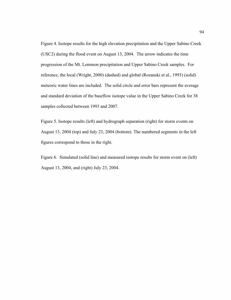
94

Figure 4. Isotope results for the high elevation precipitation and the Upper Sabino Creek

(USC2) during the flood event on August 13, 2004. The arrow indicates the time

progression of the Mt. Lemmon precipitation and Upper Sabino Creek samples. For

reference, the local (Wright, 2000) (dashed) and global (Rozanski et al., 1993) (solid)

meteoric water lines are included. The solid circle and error bars represent the average

and standard deviation of the baseflow isotope value in the Upper Sabino Creek for 38

samples collected between 1993 and 2007.

Figure 5. Isotope results (left) and hydrograph separation (right) for storm events on

August 13, 2004 (top) and July 23, 2004 (bottom). The numbered segments in the left

figures correspond to those in the right.

Figure 6. Simulated (solid line) and measured isotope results for storm event on (left)

August 13, 2004, and (right) July 23, 2004.

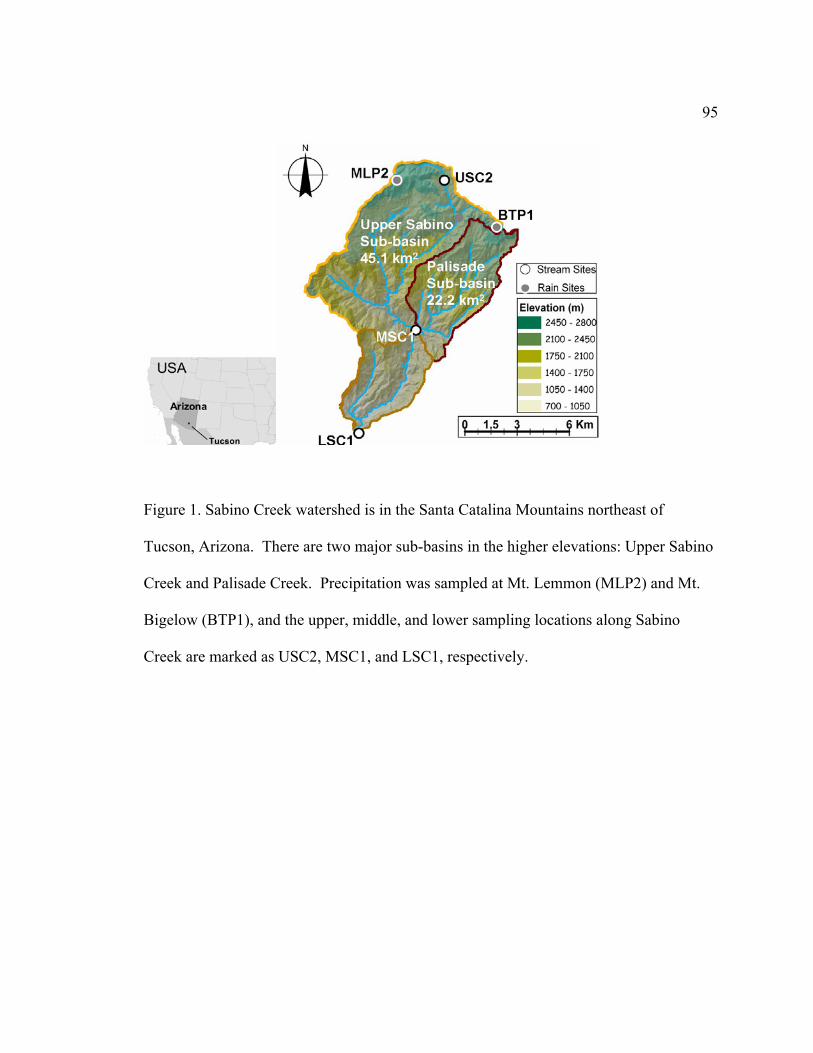
95

Figure 1. Sabino Creek watershed is in the Santa Catalina Mountains northeast of

Tucson, Arizona. There are two major sub-basins in the higher elevations: Upper Sabino

Creek and Palisade Creek. Precipitation was sampled at Mt. Lemmon (MLP2) and Mt.

Bigelow (BTP1), and the upper, middle, and lower sampling locations along Sabino

Creek are marked as USC2, MSC1, and LSC1, respectively.

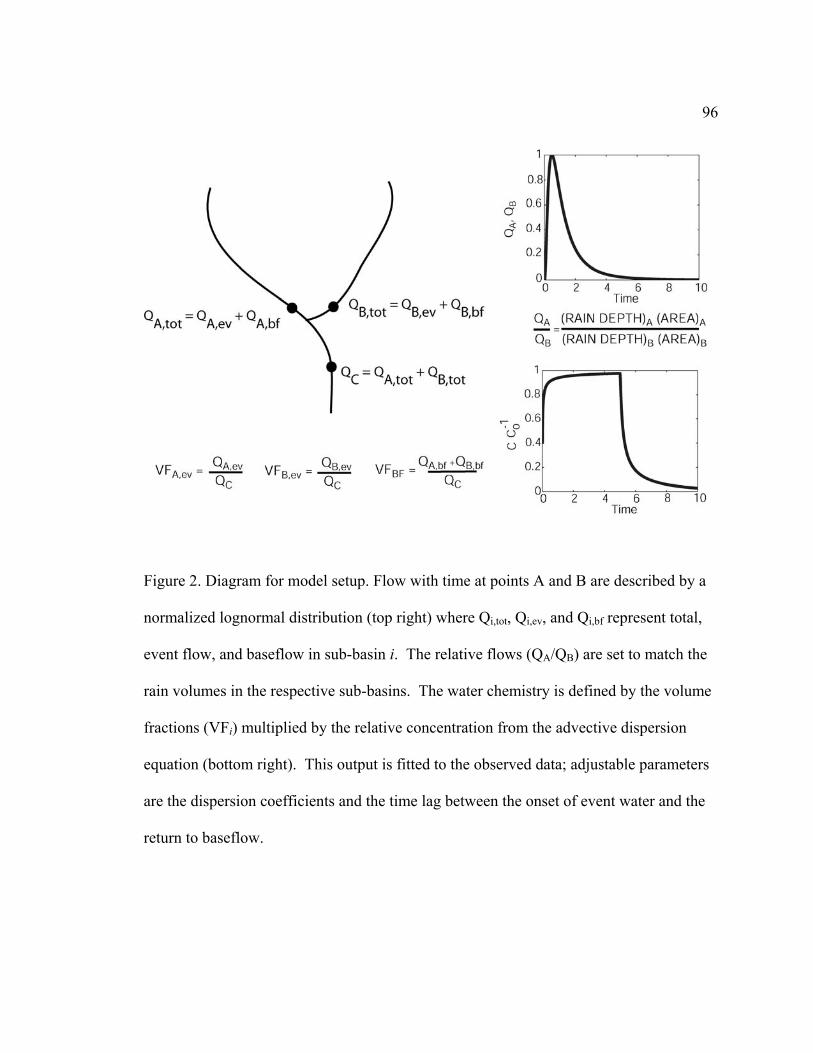
96

Figure 2. Diagram for model setup. Flow with time at points A and B are described by a

normalized lognormal distribution (top right) where Qi,tot, Qi,ev, and Qi,bf represent total,

event flow, and baseflow in sub-basin i. The relative flows (QA/QB) are set to match the

rain volumes in the respective sub-basins. The water chemistry is defined by the volume

fractions (VFi) multiplied by the relative concentration from the advective dispersion

equation (bottom right). This output is fitted to the observed data; adjustable parameters

are the dispersion coefficients and the time lag between the onset of event water and the

return to baseflow.

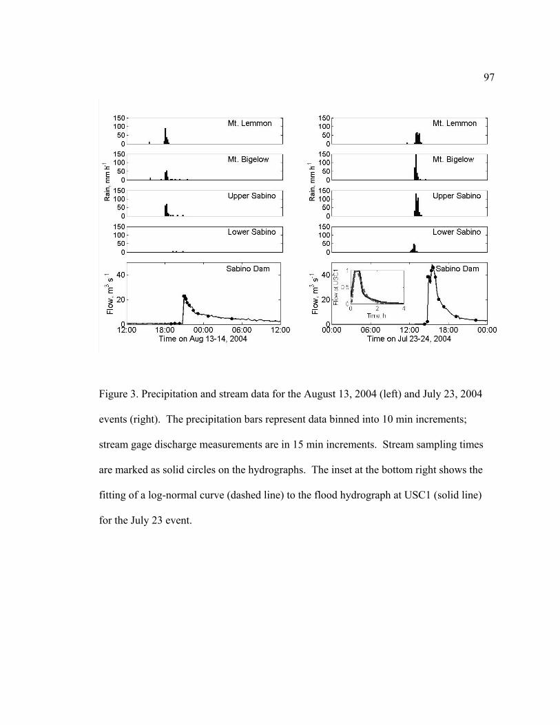
97

Figure 3. Precipitation and stream data for the August 13, 2004 (left) and July 23, 2004

events (right). The precipitation bars represent data binned into 10 min increments;

stream gage discharge measurements are in 15 min increments. Stream sampling times

are marked as solid circles on the hydrographs. The inset at the bottom right shows the

fitting of a log-normal curve (dashed line) to the flood hydrograph at USC1 (solid line)

for the July 23 event.

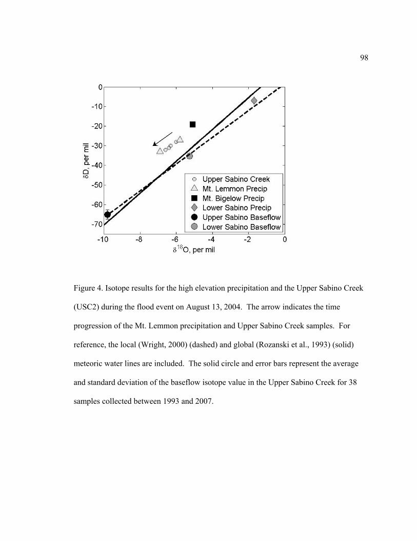
98

Figure 4. Isotope results for the high elevation precipitation and the Upper Sabino Creek

(USC2) during the flood event on August 13, 2004. The arrow indicates the time

progression of the Mt. Lemmon precipitation and Upper Sabino Creek samples. For

reference, the local (Wright, 2000) (dashed) and global (Rozanski et al., 1993) (solid)

meteoric water lines are included. The solid circle and error bars represent the average

and standard deviation of the baseflow isotope value in the Upper Sabino Creek for 38

samples collected between 1993 and 2007.

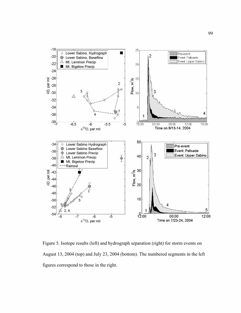
99

Figure 5. Isotope results (left) and hydrograph separation (right) for storm events on

August 13, 2004 (top) and July 23, 2004 (bottom). The numbered segments in the left

figures correspond to those in the right.

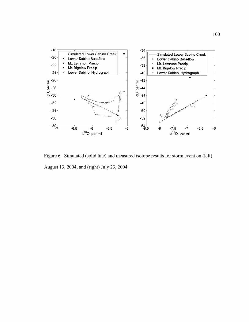
100

Figure 6. Simulated (solid line) and measured isotope results for storm event on (left)

August 13, 2004, and (right) July 23, 2004.

101

APPENDIX C

NUMERICAL SIMULATIONS OF TRANSIENT BANK STORAGE IN SEMI-ARID

STREAM-VADOSE ZONE SYSTEMS

Sharon L. E. Desilets, Ty P. A. Ferré, and Peter A. Troch

Department of Hydrology and Water Resources, University of Arizona, Tucson, Arizona.

102

Abstract

Bank storage is a critical process for maintaining low flows in many semi-arid streams.

Key questions are what conditions are necessary to recover water lost to the stream banks

during floods of relative short duration which may encounter thick unsaturated zones, and

what are the implications for semi-arid streams? We use the variable saturation code

HYDRUS 2-D (Šimůnek et al., 1999) to simulate transient flow for a wide range of flood

durations and vadose zone depths. These simulations show that during infiltration, the

wetted area around the stream bed progresses through three main characteristic behaviors

that govern infiltration and seepage behaviors. Vadose zone thickness is a critical

parameter for the spatial distribution of saturation and for potential seepage in semi-arid

streams. We provide guidelines to predict the duration and magnitude of infiltration and

seepage during these phases based on water table depth, flood stage, and flood duration

for use in estimating stream-aquifer interactions and for designing experiments. In

addition, we show that, during recession, the seepage capture zone of the stream only

extends to a small area above and below the base of the stream. For the soils used in our

simulations, no significant seepage occurs when the initial water table depth is greater

than 5 m beneath the stream base.

103

1. Introduction

Transient storage of flood water in stream banks during high flow conditions

plays a critical role in semi-arid environments. In ephemeral streams, water infiltrated

during flood events is a significant component of the water balance (Deil, 2005). Further,

bank seepage during flood recession is essential for sustaining low flows (Kondolf et al.,

1987). When groundwater tables are falling and the importance of streamflow is

evaluated with respect to environmental maintenance (Whiting, 2002), the critical role of

bank infiltration and seepage for sustaining a riparian and possibly endangered habitat

has wide implications.

In spite of the importance of this process in semi-arid environments, much of the

literature on bank storage has focused on streams in humid climates that are closely

connected to an unconfined aquifer. This condition generally does not hold in semi-arid

environments where disconnected river-aquifer systems are becoming increasingly

common due to overdraft of groundwater resources. When considering semi-arid

conditions, a deep aquifer is commonly assumed so that only streamflow losses are

considered during flooding. Desilets et al. (in submission) examine the patterns of water

exchange during the transition from connected to disconnected behavior. In this article,

we use the numerical model HYDRUS-2D (Šimunek et al., 1999) to model the rates of

bank infiltration and drainage in semi-arid environments over a range of water table

depths and flood durations.

104

2. Background

Hydrological characteristics of semi-arid rivers vary widely, but can be

generalized to distinguish them from their humid river counterparts. Semi-arid rivers

tend to have complex, braided channels with low flows, high transmission losses, and

large relative flood magnitudes that transport large quantities of unconsolidated alluvium

downstream (Nanson et al., 2002). Further, the commonly ephemeral channels have a

wide range of vadose zone depths beneath them, from perennial gaining streams

supported by locally elevated aquifer levels to unsaturated thicknesses of hundreds of

meters. These combined characteristics govern the importance of bank storage and

drainage on the hydrology and biogeochemistry of the system.

In semi-arid regions, high transmission losses are the result of severe flooding,

with typically steep rising and falling limb hydrographs, combined with a dry and often

highly permeable, unconsolidated matrix. Among several other variables, the infiltration

rate will depend on the degree of connectedness between the stream and aquifer, as this

will govern the partitioning of vertical and horizontal components of the matrix flow

(Constantz et al., 2002). Constantz et al. (2002) compared temperature-based percolation

rates below ephemeral channels with flow-gage stream loss measurements. Based on

disconnected stream-aquifer systems in three dissimilar study areas in the southwestern

United States, they attributed approximately 10% of stream losses to non-vertical vadose

zone flow. The connectedness between the stream and aquifer is more critical for

determining the quantity and composition of return flow as seepage from saturated stream

banks. In spite of the potential importance of bank seepage for stream and riparian water

105

budget and solute transport calculations, this parameter has rarely been measured in semi-

arid regions, and has not been generalized. Based on soil moisture and stream

hydrometrics, Whitaker (2000) found approximately 10% contribution from bank

discharge to the total stream flow measured for a half year time period in a gaining reach

of the San Pedro River, AZ. For losing reaches, the percent contribution of bank

discharge is expected to be much lower.

A wide range of analytical expressions for the interactions between stream stage

and bank saturation have been developed. Models for bank accretion and recession

following a sinusoidal hydrograph input were developed for one and two dimensions by

Cooper and Rorabaugh (1963) and Verma and Brutsaert (1971), respectively. Neuman

(1981) presented an equation for recession from an infinite two-dimensional aquifer

connected to a stream with an instantaneous stage change as a specific solution of his

theory on flow in unconfined aquifers (Neuman, 1972). Hunt (1990) used a perturbation

procedure for coupling a flood routing solution with groundwater flow equations. More

recently, impulse response and unit step response functions have been developed to relate

stream-aquifer flow (Hantush et al., 2002). These approaches generally require the

Dupuit assumptions that head remains constant in a vertical column and that the

hydraulic gradient is equal to the slope of the free surface. Also, most assume that the

stream is in hydrologic connection with a fully penetrating aquifer. These assumptions

are especially poor for semi-arid environments where the free surface near the bank may

be steeply sloped and where the vadose zone between the stream and the water table is

often relatively deep (greater than 5 m).

106

Numerical studies of bank storage have progressed to include more processes in

typically humid conditions. Pinder and Sauer (1971) were the first to demonstrate

numerically that bank storage will depress a flood peak and extend its tail. Whiting and

Pomeranets (1997) developed WaTab2D, a two-dimensional model for groundwater flow

with seepage based on earlier work of (Neuman and Withersp, 1970). They found the

total seepage volume is directly proportional to the floodplain width, bank height, and

specific yield; and the duration of seepage increases with increasing floodplain width and

decreasing hydraulic conductivity. Chen and Chen (2003) used MODFLOW and

MODPATH to investigate the factors controlling infiltration, release, and storage zones

associated with stream-bank interactions. They found larger flow rates and storage

volumes for larger stream-stage fluctuations, and lower infiltration rates and storage

zones with lower conductivity matrices. They observed only slight differences in bank

storage between losing and gaining streams. Chen et al. (2006) extended this work to

evaluate the importance of bank storage in baseflow separation calculations. These

numerical analyses provide a starting point for our investigations. We extend past work

by varying parameters that are critical in a semi-arid area: flood duration and vadose zone

depth. Further, we include variable saturation, which may be an important factor for the

commonly thick unsaturated zones in semi-arid locations.

In this paper we evaluate infiltration and seepage processes during flooding in

semi-arid environments. The objectives are (1) to quantify infiltration and seepage in

terms of rates, duration, cumulative values and capture zones for a wide range of

unsaturated zone depths and flood durations, (2) to describe the vadose zone processes

107

that govern the relationship among infiltration, seepage, vadose zone depth, and flood

duration, and (3) to provide guidelines to predict the duration and magnitude of

infiltration and seepage for use in estimating stream-aquifer interactions and for

designing experiments.

3. Methods

Numerical simulations were conducted with HYDRUS-2D (version 2.0) for the

transport of water in a variably saturated medium (Šimunek et al., 1999). This software

solves the two dimensional Richards equation using a Galerkin-type finite element

scheme. The modeled domain (Figure 1) is a vertical plane with a stream bank angle of

90o, stream depth of 1 m, with flood stage being full stream capacity (so). We model the

flood wave as a step function, a reasonable approximation for the narrow, steep-peaked

hydrographs common in semi-arid areas. Further, we assume that the celerity of the

flood wave in the stream is so rapid that the stream stage fluctuations can be decoupled

from the subsurface. The aquifer length is set at 30 m, which was sufficient for most

cases so that the right hand boundary did not affect the water movement during the

simulation period. For a few cases, with long flood duration, the modeled domain was

extended to 60 m. The top, bottom, right side, and left side below the stream were set as

zero-flux boundaries. The stream bank was constant head for flood stage (t1) and a

seepage face for recession (t2).

The medium is comprised of a homogeneous sand with van Genuchten

(Vangenuchten and Nielsen, 1985) parameters (α = 15.5 m-1, n = 2.68) and a saturated

108

hydraulic conductivity of Ks = 0.297 m h-1. This coarse sand was selected to provide a

maximum case for quantities of infiltration and seepage given a set flood duration and

vadose zone depth. The initial water table was set at the base of the domain to mimic

shallow bedrock, as may be expected in the mountain-front areas of semi-arid streams. It

is assumed the difference between this case and shallow water table with a deep aquifer is

insignificant. Chen and Chen (2003) found small fluctuations in regional hydraulic

gradient to have a minimal affect on seepage for streams in close connection with an

aquifer. It is expected this is similar for deep aquifers as well. They also found larger

flow rates and storage volumes for larger stream-stage fluctuations. This should

predominantly affect the initial infiltration rates, with smaller influence on the longer

time analyses associated with the deeper aquifers. The initial pressure head distribution

above the water table is hydrostatic. In semi-arid areas where soils dry quickly from

evapotranspiration, this is a reasonable assumption. If the initial condition was field

capacity, we would expect lower infiltration rates than for hydrostatic conditions, but

similar seepage in both cases.

Particle tracking was used to determine seepage capture zones. Particle tracking

calculations were based on the water velocity vectors generated by HYDRUS. A particle

was placed at every node in the domain and advanced at each time step according to the

velocity vector and time change for that step. The time increments were gradually

increased from 0.025 to 0.5 h. Seeping particles were determined as those that moved out

of the domain across the stream bank. The initial locations of these particles were

mapped to create a seepage capture zone.

109

4. Results

During the flood stage (t1 = 0 to tf), the wetted area of the vadose zone around the

stream bed progresses through three main periods of characteristic behavior (Figure 2A).

The first stage is the growth of the unobstructed infiltration bulb as defined by Philip

(1989). When the front reaches the base of the vadose zone (td) its vertical movement is

restricted. Following this time, mounding of the infiltrating water atop the water table or

impermeable layer causes increasing pressure heads to propagate upward. When the

pressure increase reaches the base of the stream (th), it causes a reduction in the

infiltration rate (Figure 2B). As infiltration continues, the wetted area moves laterally

along the bottom boundary. When the saturated wedge reaches the base of the stream

(tsbwf) the saturated width of this layer (xsbwf) begins to increase (Figure 2C). The times

associated with these three stages (td, th, and tsbwf) increase nonlinearly as the depth of the

vadose zone (d) increases (Figure 2D).

While the infiltration front is advancing vertically, the shape of the cumulative

infiltration curve corresponds with that of vertical infiltration (Figure 2B). This is

analogous to an analytical expression for vertical infiltration and represented in Figure 2B

by an aquifer that is 10 m below the base of the stream. For depths greater than 10 m

(d → ∞), the cumulative infiltration with time falls along the same line as that for d = 10

m. For depths shallower than 10 m, the rate of cumulative infiltration decreases at some

time (th) after the wetting front reaches the bottom boundary (th > td). The minimum

possible infiltration for a given flood duration occurs when the stream bank geometry has

110

a zero-flux boundary congruent with the base of the stream bed (d = 0). This is

analogous to the analytical case of horizontal absorption.

The width of the saturated area at the stream base also reflects the infiltration

stages. The width first increases rapidly at short times, then remains constant for a period

of time related to the depth of the aquifer, and then increases again as the aquifer fills

(Figure 2C). The time of the second increase (tsbwf, where sbwf is the stream base wetted

front) grows quickly with increasing vadose zone depth. Figure 2D shows the

relationship between aquifer depth and the times associated with the three stages of

infiltration: wetting front reaching the bottom boundary (td), reduction of infiltration rate

relative to vertical infiltration rate due to mounding atop the bottom boundary (th), and

the saturated wedge reaching the stream base (tsbwf). For the conditions modeled here,

these times increase slowly for shallow water table depths, and increase rapidly for water

table depths greater than 5 m.

Post-flooding seepage originates from a small area that extends symmetrically

above and below the elevation of the base of the stream. Capture zones were determined

for three initial water table depths (d = 0, 1.0, and 5.0 m) with a flood duration of 24 h

(Figure 3A), and for three flood durations (tf = 24, 48, and 72 h) with a vadose zone depth

of 1 m. The capture zone expands for increasing flood durations and decreasing vadose

zone depths. Figure 4A shows that the cumulative seepage initially increases rapidly with

time then the seepage rate decreases until a maximum cumulative seepage value is

attained and no more seepage occurs (t2 = ts). For d ≥ 1 m, ts is less than 1.5 flood

durations and decreases as the depth of the vadose zone increases (Figure 4B).

111

Total seepage decreases sharply with increasing vadose zone depth (Figure 4C).

For comparative purposes, the seepage volumes are normalized to the maximum seepage

possible for a given flood duration (Smax,d=0). This maximum potential seepage is equal to

the volume of infiltrated water stored above the horizontal plane of the stream bed. This

is equivalent to the cumulative infiltration at t = tf for the case analogous to horizontal

absorption (Id=0). In this scenario, the zero-flux bottom boundary in the stream bank is at

the same level as the stream bed. With this normalization, the simulated seepage for a

sand matrix is near 0.5 for d = 0 m and decreases to zero by d = 5 m.

Total seepage increases with increasing flood duration (Figure 4D). Initially,

there is no seepage until some time after the flood duration is sufficient to reach the

bottom boundary (tf . td-1 » 1), then there is a rapid increase with increasing flood

duration.

5. Discussion

5.1 Infiltration

Infiltration of floodwater into streambanks above a deep vadose zone can be

segmented into three phases. In the first stage, infiltration is initially and briefly

horizontal, followed by a period of vertical movement, as shown by the progression of a

saturation contour (θ = 0.4) with time for a sand matrix (Figure 2A). The duration of this

vertical infiltration stage is a function of the thickness of the vadose zone. In the second

stage, after the wetting front reaches a water table or a bottom zero-flux boundary, it

advances horizontally along this feature. Eventually, the infiltrating water fills from top

112

to bottom and forms an expanding wedge shape of saturation that extends from the top of

the stream bank to the edge of the wetting front along this feature. When the saturated

wedge reaches the base of the stream (tsbwf) the saturated width of this layer (xsbwf) begins

to increase (Figure 2C). Because of the higher root density and solute concentrations in

this region around the stream base, xsbwf and tsbwf may be critical parameters for ecosystem

management.

The time at which the infiltration rate begins to deviate from that of purely

vertical infiltration (th) is greater than td by the amount of time required for the pressure

build up to reach the stream base. This time grows faster than td at large depths (Figure

2D) because the mounding water is also dissipating laterally and has more time to do so

when the vadose zone depth is larger. The time for the saturated wedge to reach the

stream base (tsbwf) increases faster with increasing d than the other two characteristic

times. It approximately follows the square of the vadose zone depth.

The transition times for deep aquifers are disproportionately long compared to the

time for the wetting front to reach the base of the unsaturated zone (td). These times are

also generally longer than flood duration (tf). This implies that for typical flood durations

(< 50 h), infiltration into systems with a vadose zone deeper than 10 m will behave

dominantly like vertical infiltration (Figure 2A). This rule of thumb is based on a sand

matrix with a high hydraulic conductivity. For finer-grained materials, horizontal

infiltration is greater relative to vertical, the bulb-stage of infiltration is longer for a given

vadose zone depth, and the infiltrating front takes longer to reach the water table.

Therefore, the 10 m limit determined here could be considered a maximum depth for

113

which to expect to see a boundary-induced reduction of the infiltration rate. This also

implies that, for depths greater than 10 m, the extent of horizontal wetting in the area of

the stream is limited to the steady state wetting bulb. Note that, although the limiting

case for depth is set based on high permeability material, the width of this bulb will

depend on the matrix material.

The infiltration pattern will affect the type and extent of riparian vegetation that

can be supported. For aquifers < 10 m, horizontal spreading at the water table could

maintain a water supply for vegetation with shallow roots laterally distant from the

stream; however, for deep aquifers, this type of vegetation would not have a persistent

stream-supplied water supply, even within a few meters of a river after long flooding

conditions (without overbank flow conditions).

5.2 Seepage

Capture zones reveal that a relatively small region of the wetted subsurface

contributes to seepage compared to the total area that is saturated from the flooding

(Figure 4A and 4B). In vertical extent, the capture zone extends an approximately equal

distance above and below the base of the stream, ± 0.5 m for a 1 m change in stage. In

horizontal extent, the size is on the order of a couple of meters and is sensitive to the

depth of the vadose zone. With both increasing flood duration and decreasing depth

below the stream bed, the capture zone expands laterally, but largely maintains its

vertical spread. For deep aquifers, although a significant quantity of water may infiltrate,

and the total wetted region is large, the amount that returns as seepage is small. This

114

implies that the potential area for transferring accumulated solutes from the soil to the

stream is limited. Further, since solutes are commonly concentrated in the uppermost

layers of soil, they could be left behind in the soil matrix as the majority of the wetted

region is deeper (Desilets et al., in submission).

Although the total volume of seepage is generally much less than the cumulative

infiltration, the total time for flood water to seep during the recession stage (t2 = ts) can be

longer than several flood durations for shallow aquifers (d < 1 m). For d > 1 m the

seepage time is limited to 1.5 flood durations and decreases rapidly with increasing

depth. When scaled by total seepage (Stotal) and ts, the cumulative seepage curves

associated with different depths collapse to a single curve. This indicates that this

drainage behavior is independent of vadose zone depth and flood duration and suggests

that a simple, universal relationship may be developed.

The total seepage that returns to the stream decreases sharply with increasing

vadose zone depth (Figure 4C). The total seepage results are scaled by the maximum

seepage expected for a particular domain geometry and flood duration. This maximum

quantity is represented by the case where the bottom of the vadose zone is congruent with

the stream base (d = 0, dashed line in Figure 1). The simulated stream banks are

intentionally long enough so that the infiltrating water does not reach the right boundary.

For this case, with a laterally infinite aquifer, the largest fraction of water that can return

to the stream is approximately equal to half of the water that infiltrated (Figure 4C). After

the flood stage (t1 = tf, t2 = 0), a divide in the horizontal velocity vectors occurs at

approximately half the distance to the wetting front; water redistributes either toward the

115

infinite boundary or returns toward the stream. Given this scaling, the d = 0 case for each

of the flood durations is slightly greater than 0.5. As the depth of the vadose zone

increases to 5 m, this quantity decreases to zero. Similarly, the total seepage that returns

to the stream increases sharply with increasing flood durations for small vadose zone

depths, but for large depths, long floods are required to obtain even small quantities of

seepage (Figure 4D). The total seepage for various flood durations and depths can be

scaled to a single curve by normalizing the flood duration by tsbwf (Figure 4, inset). This

implies that by estimating tsbwf for a given geometry and flood duration as described in

the previous section, seepage volume and time can be estimated from Figure 4; similar

curves could be developed for other soil types.

These analyses allow us to make some general conclusions regarding limiting

behaviors of seepage in semi-arid areas. The total area of the capture zones shown here

for a coarse soil can be considered a maximum because, as conductivity decreases, total

infiltration decreases rapidly. For shallow vadose zones, the total seepage will increase

with flood duration. For the sand matrix, even for long flood durations (tf = 50 h), there

is no significant seepage returning to the stream when the vadose zone beneath the stream

bed is greater than 5 m. An estimate of the total quantity of seepage volume and time can

be obtained from Figure 4. These values can be considered a maximum for most soil

matrices because finer grained materials would move more slowly in the vertical

direction and would require even longer flood durations for mounding atop the water

table to reach the base of the stream.

116

Other factors not considered in our simulations may also affect the amount of

seepage recovered. We simplified the shape of a flood wave to a square pulse. For

many semi-arid streams, a steep rise in the hydrograph is well-represented by the square

pulse, but the recession is generally much longer. This would delay the timing and

possibly reduce the quantity of the bank water release. A low-conductivity layer in the

stream bed would reduce the infiltration rate of flood water, though this is less common

in semi-arid streams that are regularly scoured by flash floods. The distribution of the

water that does infiltrate should behave similarly to the results shown here. Additional

anisotropy would affect expectations for infiltration and seepage (e.g. Wilson and de

Cook, 1968). The most common anisotropy expected would be horizontal layering. In

this case, if a low conductivity layer is near the stream, it is expected this layer will act

similarly to the zero-fluz boundary as modeled in this study. Finally, reducing the angle

of the bank will decrease the amount of seepage recovered. This was evaluated for a set

of angles and a single scenario regarding all other parameters (10 h flood duration, 1 m

length for the angled face, and 0.75 m depth of vadose zone from the midpoint of the

angled face). The shape of the decrease was determined to be an S-curve (not shown).

For a 60o angle from the horizontal (a, Figure 1), seepage was reduced by 28%, and for a

= 30o, seepage was reduced by 80%.

6. Conclusions

The physical characteristics of semi-arid stream-streambank systems span a wide

range of conditions, the interplay of which controls the distribution of bank storage and

117

the potential for post-flood seepage. In particular, there is a balance between horizontal

and vertical processes, which is governed largely by the depth of the vadose zone beneath

the stream and duration of the flood. The extreme cases can be described as either

vertical infiltration above a deep water table or horizontal absorption above a shallow no

flow boundary. For these conditions, existing analytical solutions can be used to estimate

and visualize infiltration and seepage processes. Our numerical simulations focused on

the transitional transient cases between these extremes.

Infiltration occurs in three stages: (a) vertical growth of the infiltration bulb; (b)

mounding of infiltrating water atop a bottom horizontal boundary with upward-

propagation of a pressure head increase to the streambed, causing a reduction in the

infiltration rate; and (c) horizontal growth of a saturated wedge at the water table or lower

boundary. The times associated with these three stages (td, th, and tsbwf, respectively)

increase nonlinearly as the depth of the vadose zone increases. For vadose zones deeper

than 10 m, vertical infiltration rates are applicable and horizontal wetting is limited to the

steady state infiltration bulb.

The seepage capture zones are small, horizontally elongated areas above and

below the base of the stream. With both increasing flood duration and decreasing depth

below the stream bed, the capture zone expands laterally, but maintains its vertical

spread. The total volume of seepage is generally much less than that of infiltration, and

the total time for seepage is limited to 1.5 flood durations for d ≥ 1 m and decreases

rapidly with increasing depth. The total seepage that returns to the stream decreases

sharply with increasing vadose zone depth, from a maximum near 50% of infiltrating

118

water for d = 0 to zero seepage for d > 5 m. Similarly, the total seepage that returns to

the stream increases sharply with increasing flood durations for small vadose zone

depths. For large depths, long floods are required to obtain even small quantities of

seepage. The outcome of the seepage phase depends predictably on the infiltration phase,

and a minimum flood duration for the occurrence of seepage is set by the time for the

saturated wedge of infiltration to reach the base of the stream, tsbwf. The simulations in

this study generally provide a maximum case for infiltration and seepage estimates; finer

grained material would have significantly less infiltration and seepage, though perhaps

greater horizontal extents of increased wetting by capillarity.

The combined findings of this study may have important implications for our

conceptual models of the interactions between semi-arid streams and their riparian areas.

Semi-arid streams frequently originate in mountainous terrain, traverse canyons, and exit

at the mountain front onto deep alluvial-filled valley basins. For valley streams above a

deep vadose zone, vertical infiltration will dominate, maximum stream losses are

expected, and horizontal wetting is limited. For valley streams above a shallow water

table, infiltration and seepage will depend strongly on the vadose zone depth and the

flood duration. A depth of 5 m can be considered a maximum depth for which any

seepage can be expected, given flood durations up to 100 h. At the mountain front, there

is a rapid transition of vadose zone depths, and therefore of seepage return. The extent

and duration of seepage in this region could regulate the length of the stream that is

viable for aquatic habitats.

119

Acknowledgements

This work was funded by the NSF Science and Technology Center for Semi-arid

Hydrology and Riparian Areas (SAHRA).

120

References

Chen, X., D. Q. Y. Chen and X. H. Chen, Simulation of baseflow accounting for the effect of bank storage and its implication in baseflow separation, Journal of Hydrology, 327(3-4), 539-549, 2006.

Chen, X. and X. H. Chen, Stream water infiltration, bank storage, and storage zone changes due to stream-stage fluctuations, Journal of Hydrology, 280(1-4), 246-264, 2003.

Constantz, J., A. E. Stewart, R. Niswonger and L. Sarma, Analysis of temperature profiles for investigating stream losses beneath ephemeral channels, Water Resources Research, 38(12), 2002.

Cooper, H. H. and M. I. Rorabaugh. Ground water movements and bank storage due to flood stages in surface streams. 343-367. 1963. USGS. Water Supply Paper 1536-2. Ref Type: Serial (Book,Monograph)

Deil, U., A review on habitats, plant traits and vegetation of ephemeral wetlands - a global perspective, Phytocoenologia, 35(2-3), 533-705, 2005.

Desilets, S. L. E., T. P. A. Ferré and P. A. Troch, Hydrologic impacts of stream disconnection, Water Resources Research, In submission.

Hantush, M. M., M. Harada and M. A. Marino, Hydraulics of stream flow routing with bank storage, Journal of Hydrologic Engineering, 7(1), 76-89, 2002.

Hunt, B., An Approximation for the Bank Storage Effect, Water Resources Research, 26(11), 2769-2775, 1990.

Kondolf, G. M., L. M. Maloney and J. G. Williams, Effects of Bank Storage and Well Pumping on Base-Flow, Carmel-River, Monterey-County, California, Journal of Hydrology, 91(3-4), 351-369, 1987.

Neuman, S. P., Theory of Flow in Unconfined Aquifers Considering Delayed Response of Water Table, Water Resources Research, 8(4), 1031-&, 1972.

Neuman, S. P., Delayed Drainage in A Stream-Aquifer System, Journal of the Irrigation and Drainage Division-Asce, 107(4), 407-410, 1981.

Neuman, S. P. and P. A. Withersp, Finite Element Method of Analyzing Steady Seepage with A Free Surface, Water Resources Research, 6(3), 889-&, 1970.

Philip, J. R., Multidimensional Steady Infiltration to A Water-Table, Water Resources Research, 25(1), 109-116, 1989.

121

Pinder, G. F. and S. P. Sauer, Numerical Simulation of Flood Wave Modification Due to Bank Storage Effects, Water Resources Research, 7(1), 63-&, 1971.

Šimunek, J., M. Šejna and M. T. van Genuchten. The HYDRUS-2D software package for simulating two-dimensional movement of water, heat, and multiple solutes in variably-saturated media, version 2.0. 1999. Riverside, CA, U.S. Salinity Laboratory, USDA, ARS. Ref Type: Report

Vangenuchten, M. T. and D. R. Nielsen, On Describing and Predicting the Hydraulic-Properties of Unsaturated Soils, Annales Geophysicae, 3(5), 615-627, 1985.

Verma, R. D. and W. Brutsaert, Unsteady free surface groundwater seepage, J. Hydraul. Div. , Proc. Amer. Soc. Civ. Eng., 97(HY8), 1213-1229, 1971.

Whitaker, M. L. P., Estimating bank storage and evapotranspiration using soil physical and hydrological techniques in a gaining reach of the San Pedro River, Arizona, Ph.D. University of Arizona, Tucson, AZ, 2000.

Whiting, P. J., Streamflow necessary for environmental maintenance, Annual Review of Earth and Planetary Sciences, 30, 181-206, 2002.

Whiting, P. J. and M. Pomeranets, A numerical study of bank storage and its contribution to streamflow, Journal of Hydrology, 202(1-4), 121-136, 1997.

Wilson, L.G., and K.J. de Cook, Field observations on changes in the subsurface water regime during influent seepage in the Santa Cruz River, Water Resources Research, 4(6), 1219-1234, 1968.

122

List of Figures

Figure 1. Diagram of modeled system and flood stage where so is the height of the flood

stage, d the depth of the unsaturated zone beneath the stream bed, a the angle of the

stream bank, tf the duration of the flood, and ts the duration of seepage. The angle was set

to 90o from the horizontal for all simulations except a brief test to determine effects of

angle reductions on infiltration and seepage. Zero flux boundaries are set on the left hand

side below the stream stage and on the bottom; the right hand side boundary is also zero

flux, but the distance between the left and right hand sides (L) is set far enough (L =

30 m) that there is no affect from the right hand side on the dynamic portions of the

system.

Figure 2. (A) Contours of a near-saturated water content (θ = 0.42, θsat = 0.45) at several

times during flooding with vadose zone depth d = 7.5 m below the stream bed (y = 0,

dashed line). The time to reach the base of the unsaturated zone (td) for this aquifer is

10.9 h. (B) Cumulative infiltration during flood stage for various vadose zone depths.

(C) Saturated width into the aquifer at the base of the stream (xsbwf). (D) Relation

between the depth of the vadose zone beneath the streambed and the transitions for

vertical infiltration shape (th) and for wetting front growth at the stream base (tsbwf).

Figure 3. (A) Location of the stream bank seepage area capture zone for vadose zone

depths of 0, 1, and 5 m below the streambed. (B) Location of the capture zones for flood

durations of 24, 48, and 72 h in a domain with vadose zone depth of 1 m.

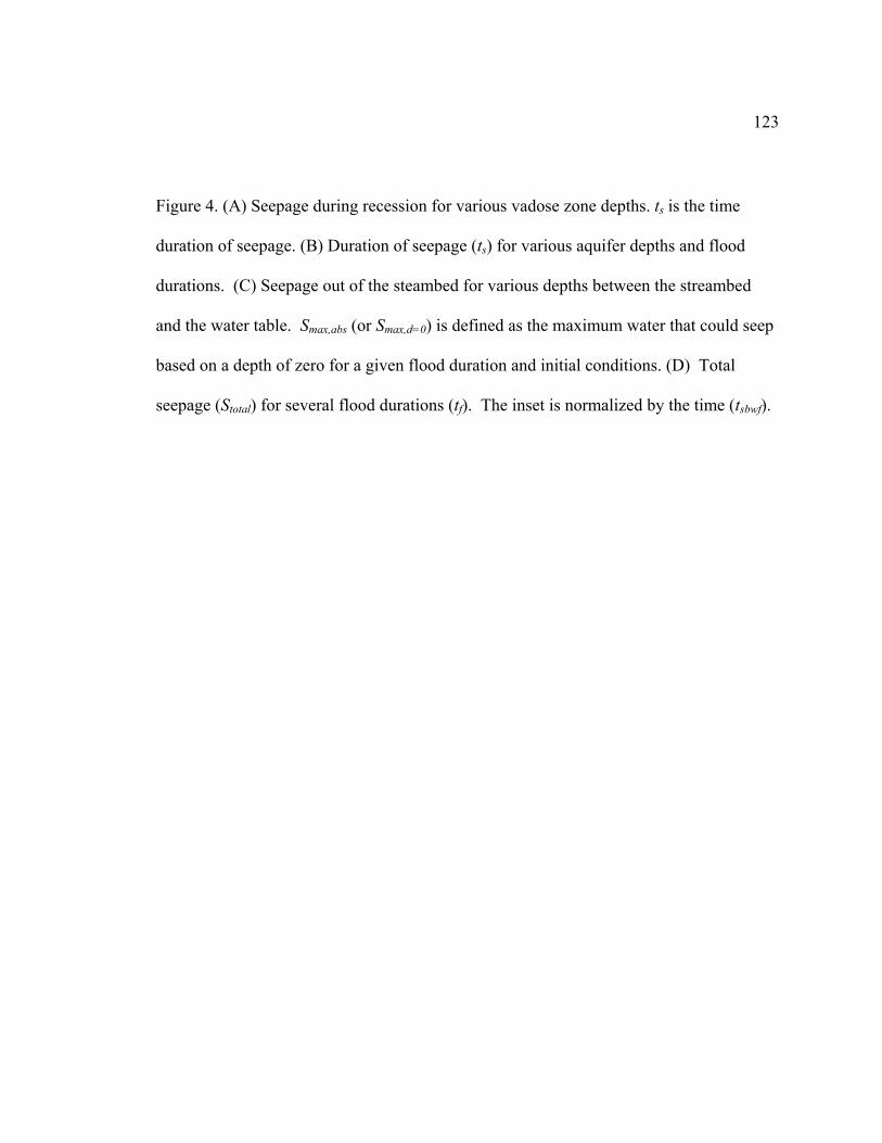
123

Figure 4. (A) Seepage during recession for various vadose zone depths. ts is the time

duration of seepage. (B) Duration of seepage (ts) for various aquifer depths and flood

durations. (C) Seepage out of the steambed for various depths between the streambed

and the water table. Smax,abs (or Smax,d=0) is defined as the maximum water that could seep

based on a depth of zero for a given flood duration and initial conditions. (D) Total

seepage (Stotal) for several flood durations (tf). The inset is normalized by the time (tsbwf).

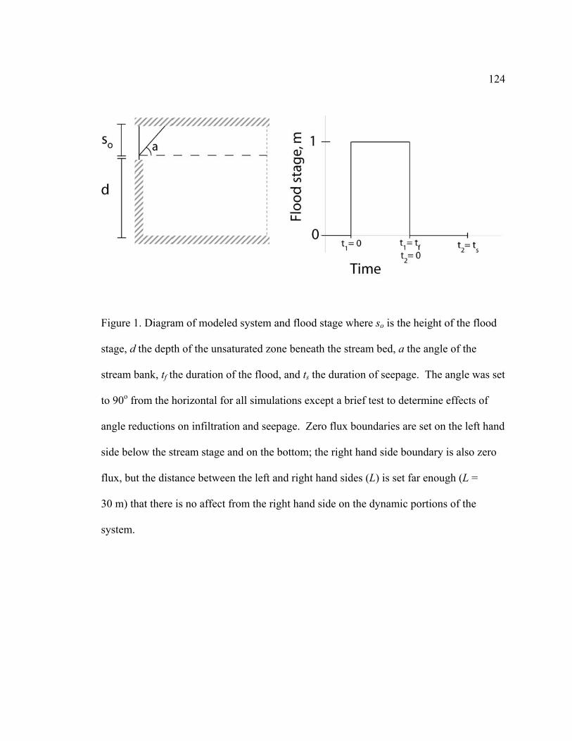
124

Figure 1. Diagram of modeled system and flood stage where so is the height of the flood

stage, d the depth of the unsaturated zone beneath the stream bed, a the angle of the

stream bank, tf the duration of the flood, and ts the duration of seepage. The angle was set

to 90o from the horizontal for all simulations except a brief test to determine effects of

angle reductions on infiltration and seepage. Zero flux boundaries are set on the left hand

side below the stream stage and on the bottom; the right hand side boundary is also zero

flux, but the distance between the left and right hand sides (L) is set far enough (L =

30 m) that there is no affect from the right hand side on the dynamic portions of the

system.

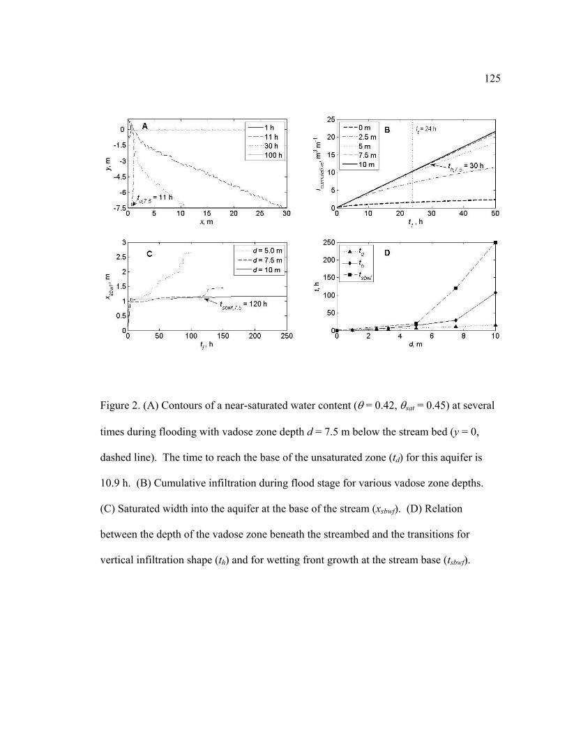
125

Figure 2. (A) Contours of a near-saturated water content (θ = 0.42, θsat = 0.45) at several

times during flooding with vadose zone depth d = 7.5 m below the stream bed (y = 0,

dashed line). The time to reach the base of the unsaturated zone (td) for this aquifer is

10.9 h. (B) Cumulative infiltration during flood stage for various vadose zone depths.

(C) Saturated width into the aquifer at the base of the stream (xsbwf). (D) Relation

between the depth of the vadose zone beneath the streambed and the transitions for

vertical infiltration shape (th) and for wetting front growth at the stream base (tsbwf).

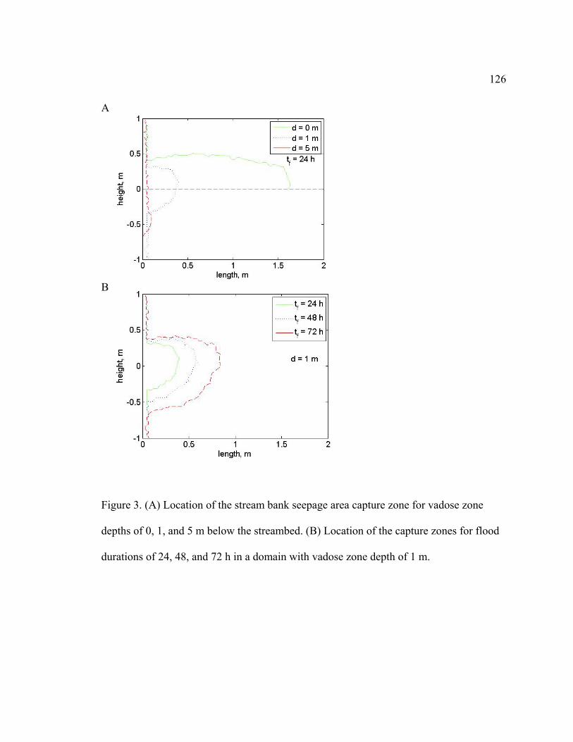
126

A

B

Figure 3. (A) Location of the stream bank seepage area capture zone for vadose zone

depths of 0, 1, and 5 m below the streambed. (B) Location of the capture zones for flood

durations of 24, 48, and 72 h in a domain with vadose zone depth of 1 m.

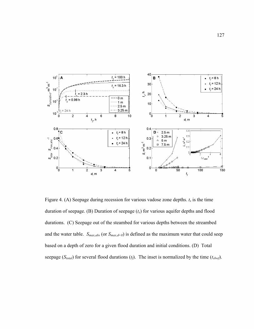
127

Figure 4. (A) Seepage during recession for various vadose zone depths. ts is the time

duration of seepage. (B) Duration of seepage (ts) for various aquifer depths and flood

durations. (C) Seepage out of the steambed for various depths between the streambed

and the water table. Smax,abs (or Smax,d=0) is defined as the maximum water that could seep

based on a depth of zero for a given flood duration and initial conditions. (D) Total

seepage (Stotal) for several flood durations (tf). The inset is normalized by the time (tsbwf).

128

APPENDIX D

HYDROLOGIC IMPACTS OF STREAM DISCONNECTION

Sharon L. E. Desilets, Ty P. A. Ferré, and Peter A. Troch

Department of Hydrology and Water Resources, University of Arizona, Tucson, Arizona.

129

Abstract Disconnected stream-aquifer systems are becoming increasingly common due to

competition for water resources and lowering of ground water tables. This work focuses

on flooding into streambanks with transitional water table depths, from a connected to a

shallow-disconnected stream-aquifer system. We use HYDRUS 2D (Šimůnek et al.,

1999) to examine rates and patterns of flow and solute transport. For even shallow

disconnections (< 1 m), we calculate more than 85% increase in infiltration losses from

the stream, elimination of post-flooding seepage, and significant increases in lateral and

vertical mixing between streamwater and antecedent pore water. Further, for the

connected stream, we demonstrate a circulation pattern at the onset of flooding that

causes an upwelling of antecedent water into the unsaturated zone. This behavior is not

produced for water table depths below 0.25 m. Our findings indicate that typical

assumptions of one dimensional, lateral flow and transport into the streambank are

incorrect.

130

1. Introduction

There is growing recognition of the importance of exchanges of water and solutes

between surface water bodies and the subsurface (Choi et al., 2000;Dahm et al.,

1998;Gooseff et al., 2002;Gooseff et al., 2007;Packman and Mackay, 2003). These

fluxes are particularly critical in riparian areas within water-stressed regions. For

example, recent studies have shown that lowering of water tables due to climate change

combined with sustained human withdrawals have led to die off of long-lived riparian

species (Cooper et al., 2006;Naumburg et al., 2005;Sarr and Hibbs, 2007). These studies

demonstrated a correlation between water table depth and riparian vegetation morbidity.

Most studies of the interaction of surface water and groundwater in streambanks

make use of one of two limiting simplifying assumptions. Either, they assume that the

stream is connected to the groundwater system (Huth, 2003;Kondolf et al.,

1987;Whitaker, 2000;Whiting and Pomeranets, 1997), or they assume that the water table

is far below the stream (Constantz et al., 2002;Niswonger et al., 2005;Ronan et al., 1998).

The former case is typically conceptualized as lateral flow from the stream to the

streambank during flooding, followed by lateral return flow to the stream, via seepage,

during recession. The latter case is conceptualized as predominantly vertical flow during

flooding with no return flow to the stream. Analytical solutions are available for these

two end member conditions (Hunt, 1990;Neuman, 1981;Philip, 1989;Vaquez-Sune et al.,

2007). We examine in more detail the changes in the rates and patterns of water and

solute flux that occur as the water table elevation decreases, causing a stream to transition

131

from an initial connected condition to a state of disconnection with the underlying

aquifer.

2. Methods

We use a numerical model of water flow and solute transport (Šimunek et al.,

1999) to examine the response to a 6 hour step-function flooding event followed by 48

hours of redistribution. We focus on three features: water loss from the stream during

flooding; seepage to the stream following flooding; and the spatial distribution of stream

water in the subsurface following flooding and following two days of redistribution. We

consider an initially flat lying water table, and examine the impacts of changes in the

water table depth below the base of the stream on these three behaviors.

To focus on interactions between the streambank and seepage face, we model a

vertical cross section, with the left boundary located at the midpoint of an infinitely

narrow stream. The domain is 6 m in the vertical and 15 m in the horizontal. The datum

elevation is located at the base of the stream. The stream is represented as a vertical line

segment along the left boundary extending from 0 m to 1 m (the elevation of the ground

surface). The left boundary below the stream is set to zero flux for water flow and for

solute transport to represent a symmetry boundary. The stream segment of the left

boundary is set to a constant hydraulic head of 0.4 m during flooding. The stream

boundary segment has a seepage face condition following flooding. In HYDRUS 2D a

seepage face maintains a hydraulic head of zero and water that crosses the boundary is

considered to be immediately removed, as by stream flow. The bottom (z = -5 m) and top

132

(z = 1 m) boundaries are zero flux for water and solute. A distant right boundary (x =

15 m) is also zero flux.

The medium is comprised of a homogeneous sand with van Genuchten

(Vangenuchten and Nielsen, 1985) parameters (α = 15.5 m-1, n = 2.68) and a saturated

hydraulic conductivity of Ks = 0.297 m h-1. The maximum initial water table height is z =

0 m, representing a stream that is minimally connected to groundwater. We then examine

increasing water table depths, to a maximum of 2.0 m. We use the solute transport

modeling capabilities of HYDRUS to track the movement of stream water (assigned a

relative concentration of 0) and antecedent pore water (assigned a relative concentration

of 1). Concentration is defined as solute mass per volume of pore water. We assign

longitudinal and transverse dispersion constants of αL = 0.5 m and αT = 0.1 m. However,

we set the diffusion coefficient to zero to avoid unreasonably large diffusive mass fluxes

due to the large difference in relative concentrations in the stream water and antecedent

pore water.

3. Results

Consistent with results published previously (Niswonger et al., 2005), cumulative

infiltration during flooding is higher for disconnected streams than for connected streams

(solid line, Figure 1). Our results show that the cumulative infiltration transitions

nonlinearly, with relatively large changes occurring with the initial disconnection of the

stream and aquifer. In fact, if the initial water table depth is one meter below the

133

streambed, the cumulative infiltration is 89% of the amount that would occur for an

infinitely deep water table, for our flooding scenario.

In all cases, added water causes the water table to rise near the stream and extend

as a wedge, laterally away from the stream (Figure 2, left column). For the conditions that

we examined, water table rise near the stream led to nonzero seepage (difference between

the solid and dashed lines, Figure 1) for an initial water table depth of 0.25 m or less.

The net water flux to the subsurface through flooding and redistribution was highly

nonlinear. That is, even a small disconnection between the stream and the underlying

aquifer led to a much greater net loss of water from the stream (dashed line, Figure 1)

throughout a flooding event.

The spatial distribution of streamwater following flooding (t2 = 0 h) and after 48

hours of recovery (t2 = 48 h) show the subsurface zone that is affected by streamwater

exchange (Figure 2, right column). We show two contour levels: 0.1 represents

essentially unmixed streamwater; 0.9 represents essentially unmixed antecedent pore

water. The area between these contours represents a zone of mixed streamwater and

antecedent pore water. If the initial water table depth is located at the base of the stream

(d = 0.0 m), there is essentially no region of unmixed stream water. The mixing zone

extends horizontally approximately 1.7 m from the streambank and vertically to a

maximum depth of 1.2 m. There is little or no change in the mixing zone during

redistribution due to the significant water flow toward the seepage face. If the initial

water table depth is lowered by 0.25 m (d = 0.25 m), there is still no region of unmixed

stream water. But, the increased cumulative infiltration extends the mixing zone

134

horizontally approximately 2.0 m from the streambank and vertically to a maximum

depth of 1.6 m. There is continued downward and rightward expansion of the mixing

zone during redistribution as the water table flattens (Figure 2B, left panel). As the initial

water table depth increases to 2 m, there are significant changes in the distributions of

stream water and antecedent pore water. Unmixed stream water extends to a lateral

distance of 0.7 m and vertically to a depth of 1.1 m. The mixing zone extends vertically

in the shallow subsurface, then laterally at and above the initial water table depth. The

lateral extent of the mixing zone is much greater (2.1 m after flooding), in part due to the

increased cumulative infiltration. Finally, there is significant solute transport during

recovery (mixing zone extends to 3.1 m).

To examine the change in distribution of the antecedent pore water following

flooding and two days of drainage, we calculated the change in solute mass throughout

the domain. The streamwater has a concentration of 0.0 and the antecedent pore water

has a concentration of 1.0. Therefore, a decrease in solute mass represents a decrease in

water content and/or a decrease in the mass fraction of the antecedent pore water. An

increase in solute mass represents an increase in water content and/or an increase in the

mass fraction of the antecedent pore water. As expected, there is a large region of

decreased concentration as a result of flooding (not shown). Unexpectedly, there is a

region of increased concentration in the streambank, above the base of the stream (Figure

3A). Examination of the flow vectors at the onset of flooding (Figure 3B) shows that the

cause of this increase is upwelling of water from beneath the initial water table depth in

response to mounding beneath the stream. Conceptually, this means that the leading edge

135

water content increase in the streambank is comprised of antecedent water, not

streamwater. The streamwater moves vertically downward and mixes in higher water

content regions of the subsurface. This helps to explain why there is no significant region

of unmixed streamwater after flooding for shallow initial water table conditions (Figure

2A and 2B, right). To summarize the changes in the distribution of antecedent pore water

above the base of the stream, we calculated the change in mass of the antecedent water

compared to the mass before flooding (Figure 3C). For the connected stream (d = 0.0),

there is a significant increase in the amount of antecedent water present immediately

following flooding. However, most of this water drains out as seepage after two days of

redistribution. If the initial water table depth is decreased by 0.25 m, there is a similar

increase in antecedent water mass above the base of the stream. However, under these

conditions, the mass of antecedent water continues to increase as the water table mound

redistributes laterally following flooding. The disconnection, though small, significantly

limits loss to seepage so the net solute gain persists. Once the water table is lowered to at

least 50 cm below the base of the stream, there is a net loss of antecedent water mass due

to vertical displacement by streamwater.

4. Conclusions

We present a preliminary numerical investigation of the changes in response of a

stream-aquifer system due to lowering of the water table below the base of the stream

(stream disconnection). There are three primary changes that occur when the water table

elevation drops from the base of the stream to a depth of 0.25 m below the stream. First,

136

there is a significant increase in cumulative infiltration and an associated decrease in

seepage return, leading to much larger water loss from the stream to the streambank over

the course of flooding and drainage. Second, there is an increase in the lateral and

vertical extents of the zone of mixing of streamwater and antecedent pore water.

Furthermore, this zone continues to expand during drainage, unlike with connected

conditions. Third, while there is a decrease in the amount of upwelling of antecedent

water into the streambank, there is a more significant decrease in the rate of redistribution

of that antecedent water. As a result, more antecedent water is redistributed into the

streambank, above the base of the stream.

While the magnitudes and timings of the responses seen in our modeling study

will vary for specific site conditions, we expect that they will be present to some degree

in most systems. Therefore, we recommend that researchers who are interested in

processes that rely on water and solute exchange between a stream and the streambank

should consider the processes shown here when designing experiments. In particular, our

findings suggest that assumptions of one dimensional, lateral flow and transport into the

streambank are incorrect. This suggests that water content (or pressure) and solute

concentration should be measured at multiple depths in the streambank to fully

characterize stream/aquifer interactions.

137

References

Choi, J., J. W. Harvey and M. H. Conklin, Characterizing multiple timescales of stream and storage zone interaction that affect solute fate and transport in streams, Water Resources Research, 36(6), 1511-1518, 2000.

Constantz, J., A. E. Stewart, R. Niswonger and L. Sarma, Analysis of temperature profiles for investigating stream losses beneath ephemeral channels, Water Resources Research, 38(12), 2002.

Cooper, D. J., J. Dickens, N. T. Hobbs, L. Christensen and L. Landrum, Hydrologic, geomorphic and climatic processes controlling willow establishment in a montane ecosystem, Hydrological Processes, 20(8), 1845-1864, 2006.

Dahm, C. N., N. B. Grimm, P. Marmonier, H. M. Valett and P. Vervier, Nutrient dynamics at the interface between surface waters and groundwaters, Freshwater Biology, 40(3), 427-451, 1998.

Gooseff, M. N., R. O. Hall and J. L. Tank, Relating transient storage to channel complexity in streams of varying land use in Jackson Hole, Wyoming, Water Resources Research, 43(1), 2007.

Gooseff, M. N., D. M. McKnight, W. B. Lyons and A. E. Blum, Weathering reactions and hyporheic exchange controls on stream water chemistry in a glacial meltwater stream in the McMurdo Dry Valleys, Water Resources Research, 38(12), 2002.

Hunt, B., An Approximation for the Bank Storage Effect, Water Resources Research, 26(11), 2769-2775, 1990.

Huth, A. K., Geochemical and isotopic mixing models: Two case studies in a snow-dominated and semi-arid environment, Ph.D. University of Arizona, Tucson, AZ, 2003.

Kondolf, G. M., L. M. Maloney and J. G. Williams, Effects of Bank Storage and Well Pumping on Base-Flow, Carmel-River, Monterey-County, California, Journal of Hydrology, 91(3-4), 351-369, 1987.

Naumburg, E., R. Mata-Gonzalez, R. G. Hunter, T. Mclendon and D. W. Martin, Phreatophytic vegetation and groundwater fluctuations: A review of current research and application of ecosystem response modeling with an emphasis on Great Basin vegetation, Environmental Management, 35(6), 726-740, 2005.

Neuman, S. P., Delayed Drainage in A Stream-Aquifer System, Journal of the Irrigation and Drainage Division-Asce, 107(4), 407-410, 1981.

138

Niswonger, R. G., D. E. Prudic, G. Pohll and J. Constantz, Incorporating seepage losses into the unsteady streamflow equations for simulating intermittent flow along mountain front streams, Water Resources Research, 41(6), 2005.

Packman, A. I. and J. S. Mackay, Interplay of stream-subsurface exchange, clay particle deposition, and streambed evolution, Water Resources Research, 39(4), 2003.

Philip, J. R., Multidimensional Steady Infiltration to A Water-Table, Water Resources Research, 25(1), 109-116, 1989.

Ronan, A. D., D. E. Prudic, C. E. Thodal and J. Constantz, Field study and simulation of diurnal temperature effects on infiltration and variably saturated flow beneath an ephemeral stream, Water Resources Research, 34(9), 2137-2153, 1998.

Sarr, D. A. and D. E. Hibbs, Multiscale controls on woody plant diversity in western Oregon riparian forests, Ecological Monographs, 77(2), 179-201, 2007.

Šimunek, J., M. Šejna and M. T. van Genuchten. The HYDRUS-2D software package for simulating two-dimensional movement of water, heat, and multiple solutes in variably-saturated media, version 2.0. 1999. Riverside, CA, U.S. Salinity Laboratory, USDA, ARS. Ref Type: Report

Vangenuchten, M. T. and D. R. Nielsen, On Describing and Predicting the Hydraulic-Properties of Unsaturated Soils, Annales Geophysicae, 3(5), 615-627, 1985.

Vaquez-Sune, E., B. Capino, E. Abarca and J. Carrera, Estimation of recharge from floods in disconnected stream-aquifer systems, Ground Water, 45(5), 579-589, 2007.

Whitaker, M. L. P., Estimating bank storage and evapotranspiration using soil physical and hydrological techniques in a gaining reach of the San Pedro River, Arizona, Ph.D. University of Arizona, Tucson, AZ, 2000.

Whiting, P. J. and M. Pomeranets, A numerical study of bank storage and its contribution to streamflow, Journal of Hydrology, 202(1-4), 121-136, 1997.

139

List of Figures Figure 1. Cumulative infiltration (I) after 6 h flood (solid circles and line), and the

difference between cumulative infiltration and cumulative seepage (S) after an additional

48 h of drainage (open circles and dashed line) as a function of the initial water table

depth.

Figure 2. Contours of water content (θ = 0.4, 93% saturated) (left) and relative solute

concentration (right) following a 6 h flood (dashed lines) and after an additional 48 h of

drainage (solid lines). Initial solute concentrations are1.0 in the soil water and 0 in the

infiltrating flood water. The 0.9 and 0.1 contours delineate a zone of mixing between the

resident and infiltrating water. Results are shown for initial water table depths of (A) 0,

(B) 0.25, and (C) 2 m below the base of the stream.

Figure 3. (A) Zones of increased solute mass for the minimally connected case (d = 0 m).

Infiltrating water has zero solute mass, so plume represents movement of antecedent pore

water into the unsaturated area. Contours are shown for dM = 0.05 where dM = (Mf –

Mi)/Mi following a 6 h flood (dashed line) and 48 h of additional drainage (solid line).

The gain in mass resulted from a circulation pattern initiated by infiltrating water that

moved resident water from beneath the streambed up into the area of the streambed. (B)

Velocity vectors (d = 0) show infiltrating water moving downward, causing resident soil

water to advance upward into the previously unsaturated stream bank. A stretching factor

of 5 was used for the vertical component of the velocity. (C) Relative change in solute

140

mass in the stream bank (dMrz where subscript rz represents root zone) for several depths

following flooding and redistribution.

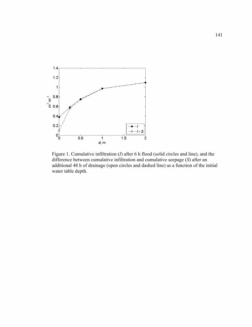
141

Figure 1. Cumulative infiltration (I) after 6 h flood (solid circles and line), and the difference between cumulative infiltration and cumulative seepage (S) after an additional 48 h of drainage (open circles and dashed line) as a function of the initial water table depth.

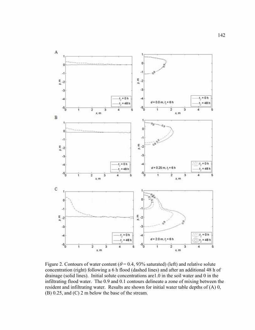
142

Figure 2. Contours of water content (θ = 0.4, 93% saturated) (left) and relative solute concentration (right) following a 6 h flood (dashed lines) and after an additional 48 h of drainage (solid lines). Initial solute concentrations are1.0 in the soil water and 0 in the infiltrating flood water. The 0.9 and 0.1 contours delineate a zone of mixing between the resident and infiltrating water. Results are shown for initial water table depths of (A) 0, (B) 0.25, and (C) 2 m below the base of the stream.

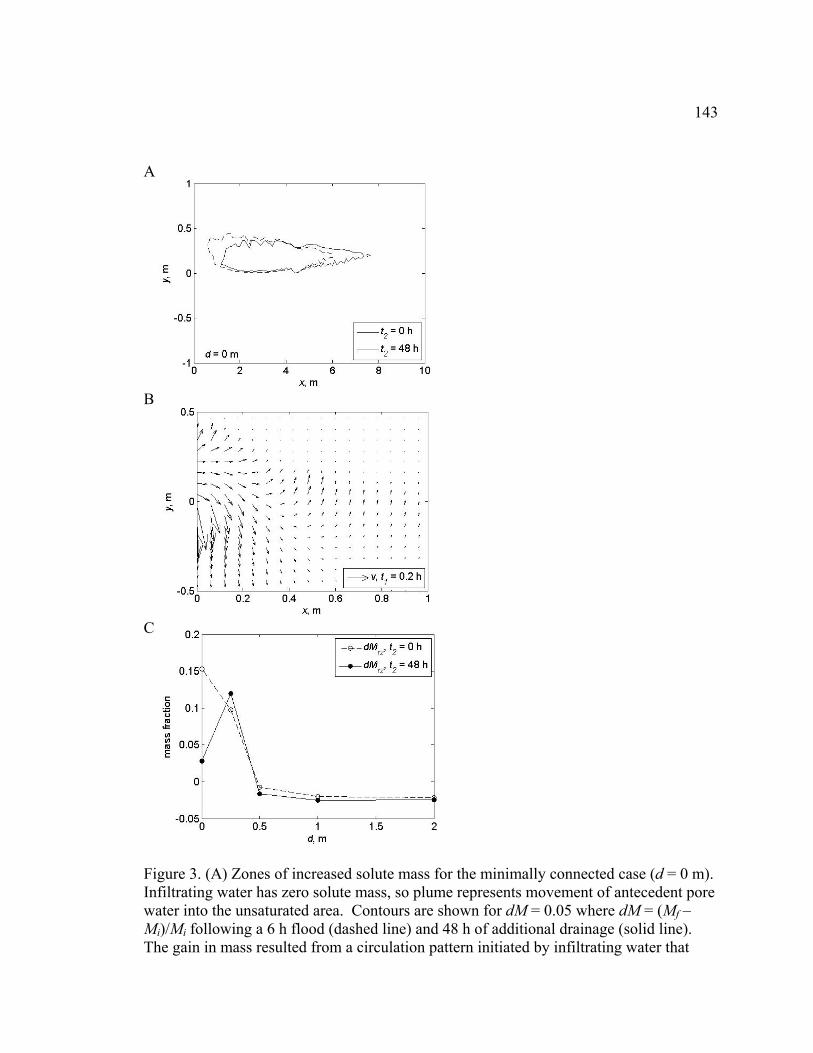
143

A

B

C

Figure 3. (A) Zones of increased solute mass for the minimally connected case (d = 0 m). Infiltrating water has zero solute mass, so plume represents movement of antecedent pore water into the unsaturated area. Contours are shown for dM = 0.05 where dM = (Mf – Mi)/Mi following a 6 h flood (dashed line) and 48 h of additional drainage (solid line). The gain in mass resulted from a circulation pattern initiated by infiltrating water that

144

moved resident water from beneath the streambed up into the area of the streambed. (B) Velocity vectors (d = 0) show infiltrating water moving downward, causing resident soil water to advance upward into the previously unsaturated stream bank. A stretching factor of 5 was used for the vertical component of the velocity. (C) Relative change in solute mass in the stream bank (dMrz where subscript rz represents root zone) for several depths following flooding and redistribution.