flexible and scalable methods for time-series...
TRANSCRIPT
Flexible and Scalable Methods for Time-Series
CharacterizationDr. Andrew Becker!
Associate Research Professor!University of Washington!
Department of Astronomy

Motivation
2
Motivation
2
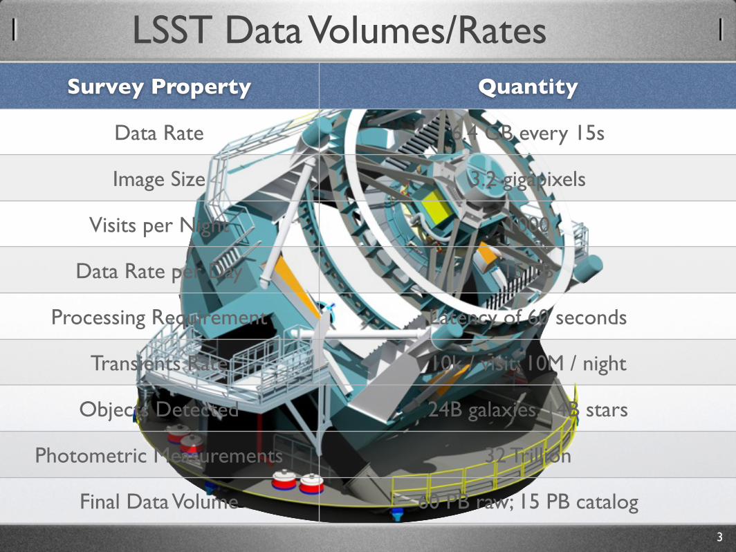
LSST Data Volumes/Rates
3
Survey Property Quantity
Data Rate 6.4 GB every 15s
Image Size 3.2 gigapixels
Visits per Night 1000
Data Rate per Day 15 TB
Processing Requirement Latency of 60 seconds
Transients Rate 10k / visit; 10M / night
Objects Detected 24B galaxies, 14B stars
Photometric Measurements 32 Trillion
Final Data Volume 60 PB raw; 15 PB catalog

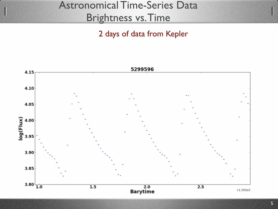
Astronomical Time-Series Data!Brightness vs. Time
1 year of data on variable star from Kepler spacecraft
4
5
2 days of data from Kepler
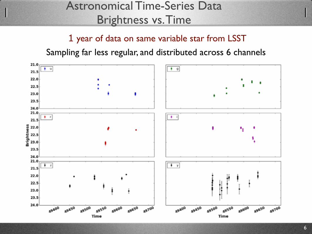
Astronomical Time-Series Data!Brightness vs. Time
6
1 year of data on same variable star from LSST
Sampling far less regular, and distributed across 6 channels
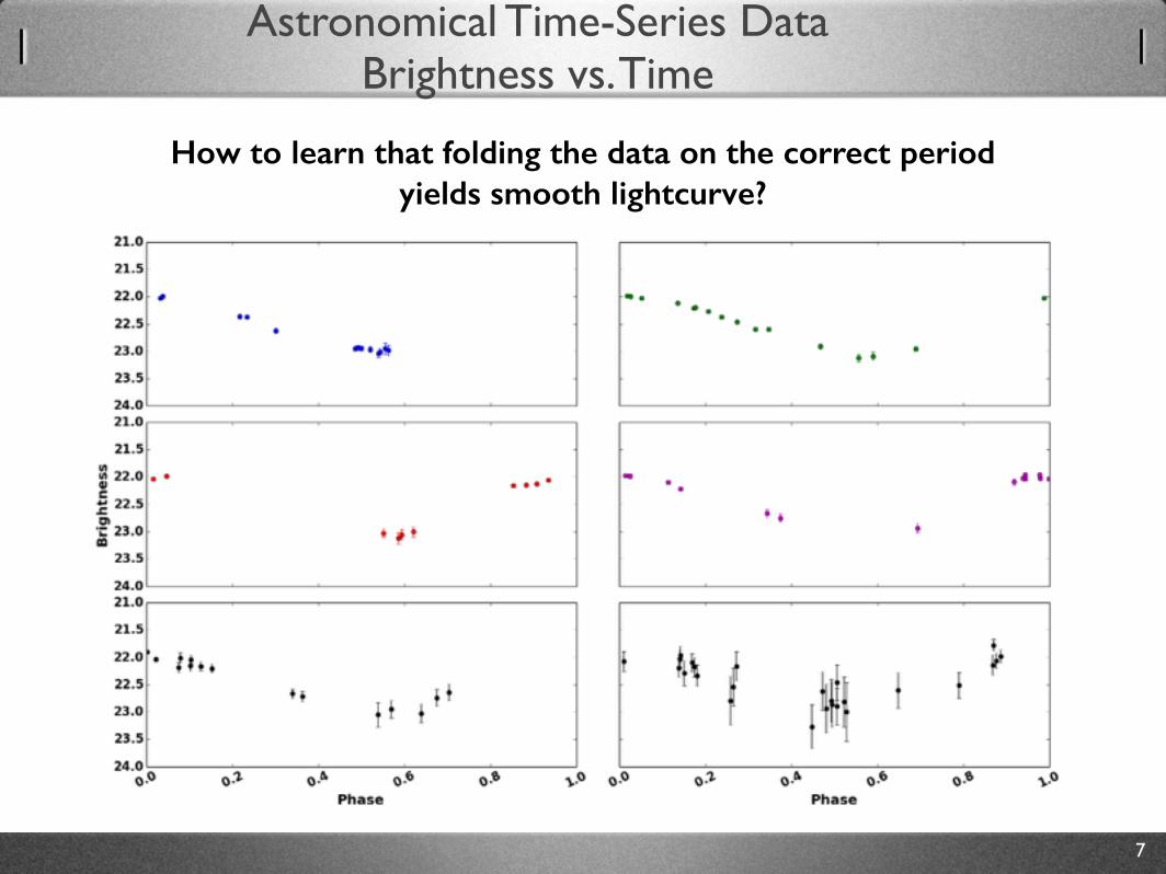
Astronomical Time-Series Data!Brightness vs. Time
7
How to learn that folding the data on the correct period yields smooth lightcurve?
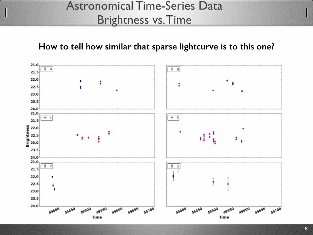
Astronomical Time-Series Data!Brightness vs. Time
8
How to tell how similar that sparse lightcurve is to this one?
Astronomical Time-Series Data!Brightness vs. Time
Lightcurve Classification
9
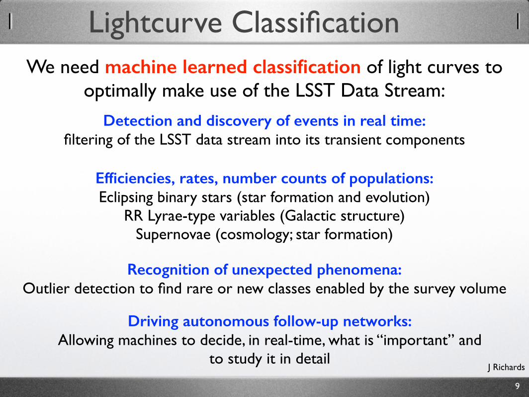
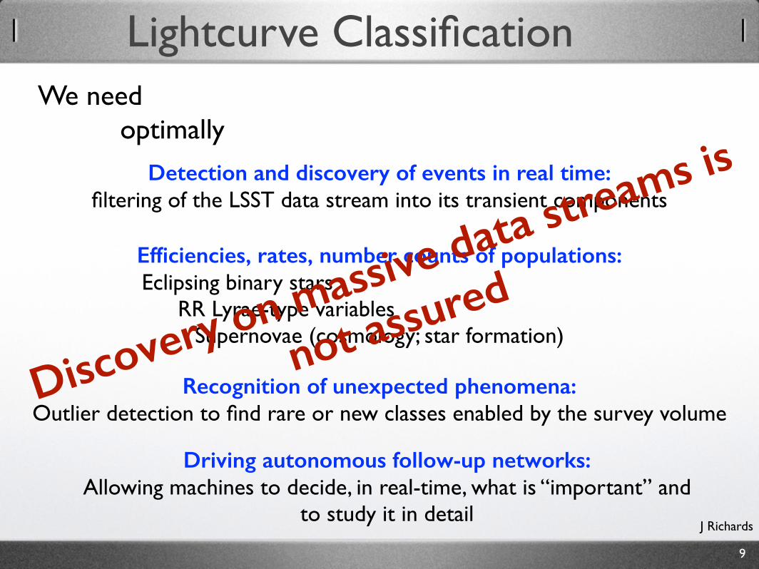
We need machine learned classification of light curves to optimally make use of the LSST Data Stream:
Detection and discovery of events in real time: filtering of the LSST data stream into its transient components
Efficiencies, rates, number counts of populations: Eclipsing binary stars (star formation and evolution)!
RR Lyrae-type variables (Galactic structure)!Supernovae (cosmology; star formation)
Recognition of unexpected phenomena: Outlier detection to find rare or new classes enabled by the survey volume
Driving autonomous follow-up networks: Allowing machines to decide, in real-time, what is “important” and
to study it in detailJ Richards
Lightcurve Classification
9
We need optimally
Detection and discovery of events in real time: filtering of the LSST data stream into its transient components
Efficiencies, rates, number counts of populations: Eclipsing binary stars
RR Lyrae-type variables Supernovae (cosmology; star formation)
Recognition of unexpected phenomena: Outlier detection to find rare or new classes enabled by the survey volume
Driving autonomous follow-up networks: Allowing machines to decide, in real-time, what is “important” and
to study it in detailJ Richards
Discovery on massive data streams is
not assured
Astrophysics as Applied Machine Learning
10
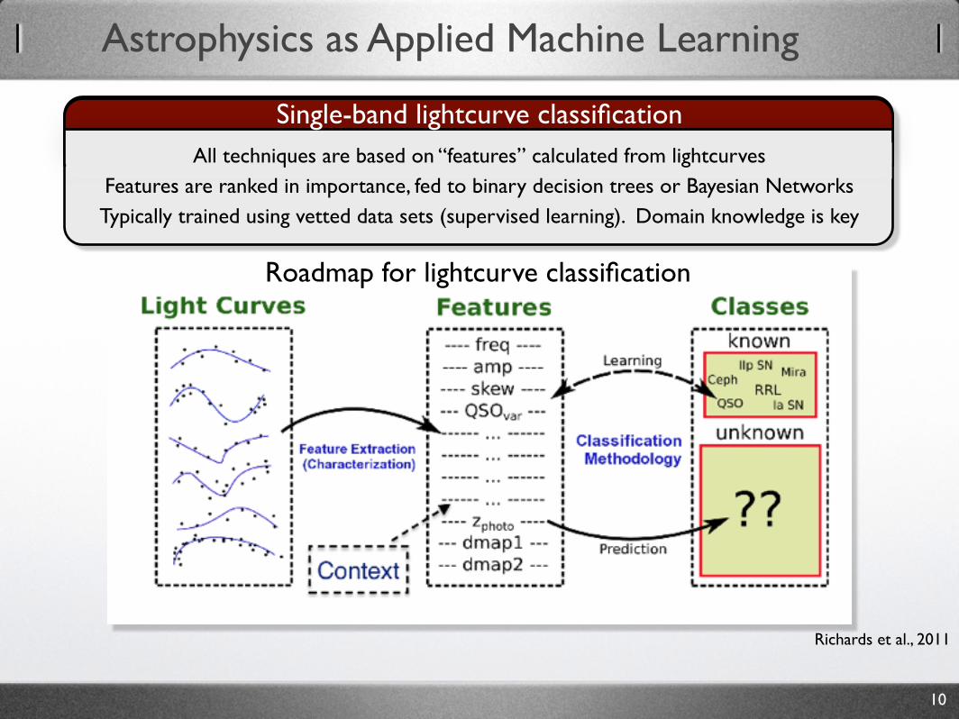
Single-band lightcurve classificationAll techniques are based on “features” calculated from lightcurves!
Features are ranked in importance, fed to binary decision trees or Bayesian Networks!Typically trained using vetted data sets (supervised learning). Domain knowledge is key
Roadmap for lightcurve classification
Richards et al., 2011
Astrophysics as Applied Machine Learning
10
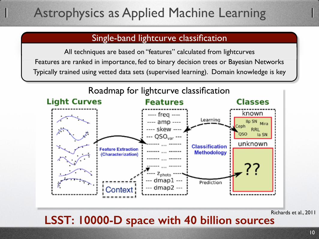
Single-band lightcurve classificationAll techniques are based on “features” calculated from lightcurves!
Features are ranked in importance, fed to binary decision trees or Bayesian Networks!Typically trained using vetted data sets (supervised learning). Domain knowledge is key
Roadmap for lightcurve classification
Richards et al., 2011
LSST: 10000-D space with 40 billion sources
11
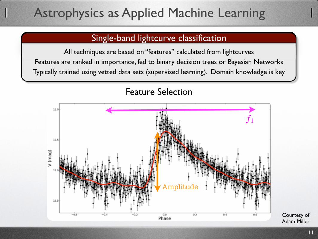
Single-band lightcurve classificationAll techniques are based on “features” calculated from lightcurves!
Features are ranked in importance, fed to binary decision trees or Bayesian Networks!Typically trained using vetted data sets (supervised learning). Domain knowledge is key
Feature Selection
Courtesy of!Adam Miller
Amplitude
f1
Astrophysics as Applied Machine Learning
12
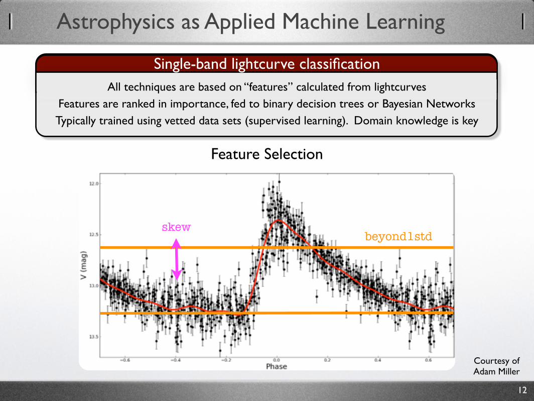
Single-band lightcurve classificationAll techniques are based on “features” calculated from lightcurves!
Features are ranked in importance, fed to binary decision trees or Bayesian Networks!Typically trained using vetted data sets (supervised learning). Domain knowledge is key
Feature Selection
beyond1stdskew
Courtesy of!Adam Miller
Astrophysics as Applied Machine Learning
13
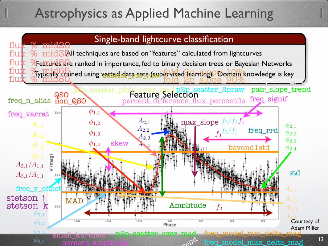
Single-band lightcurve classificationAll techniques are based on “features” calculated from lightcurves!
Features are ranked in importance, fed to binary decision trees or Bayesian Networks!Typically trained using vetted data sets (supervised learning). Domain knowledge is key
Feature Selection
beyond1stdskew
Amplitude
freq_signif
f1A1,1
A1,2
A1,3
A1,4
�1,1
�1,2
�1,3
�1,4
�2,1
�2,2
�2,3
�2,4
�3,1
�3,2
�3,3
�3,4
A3,1
A3,2
A3,3
A3,4
A2,1
A2,2
A2,3
A2,4
f2
f3
f2/f1f3/f1
A2,1/A1,1
A3,1/A1,1
freq_varrat
freq_y_offset
freq_model_max_delta_magfreq_model_min_delta_mag
freq_rrd
freq_n_alias
flux_%_mid20flux_%_mid35flux_%_mid50flux_%_mid65flux_%_mid80
linear_
trend
max_slope
MAD
median_buffer_range_percentage
pair_slope_trend
percent_amplitude
percent_difference_flux_percentileQSOnon_QSO
std
small_kurtosis
stetson_jstetson_k
scatter_res_raw
p2p_scatter_2praw
p2p_scatter_over_mad
p2p_scatter_pfold_over_madmedperc90_p2_p
fold_2p_slope_10%fold_2p_slope_90%
p2p_ssqr_diff_over_var
Courtesy of!Adam Miller
Astrophysics as Applied Machine Learning
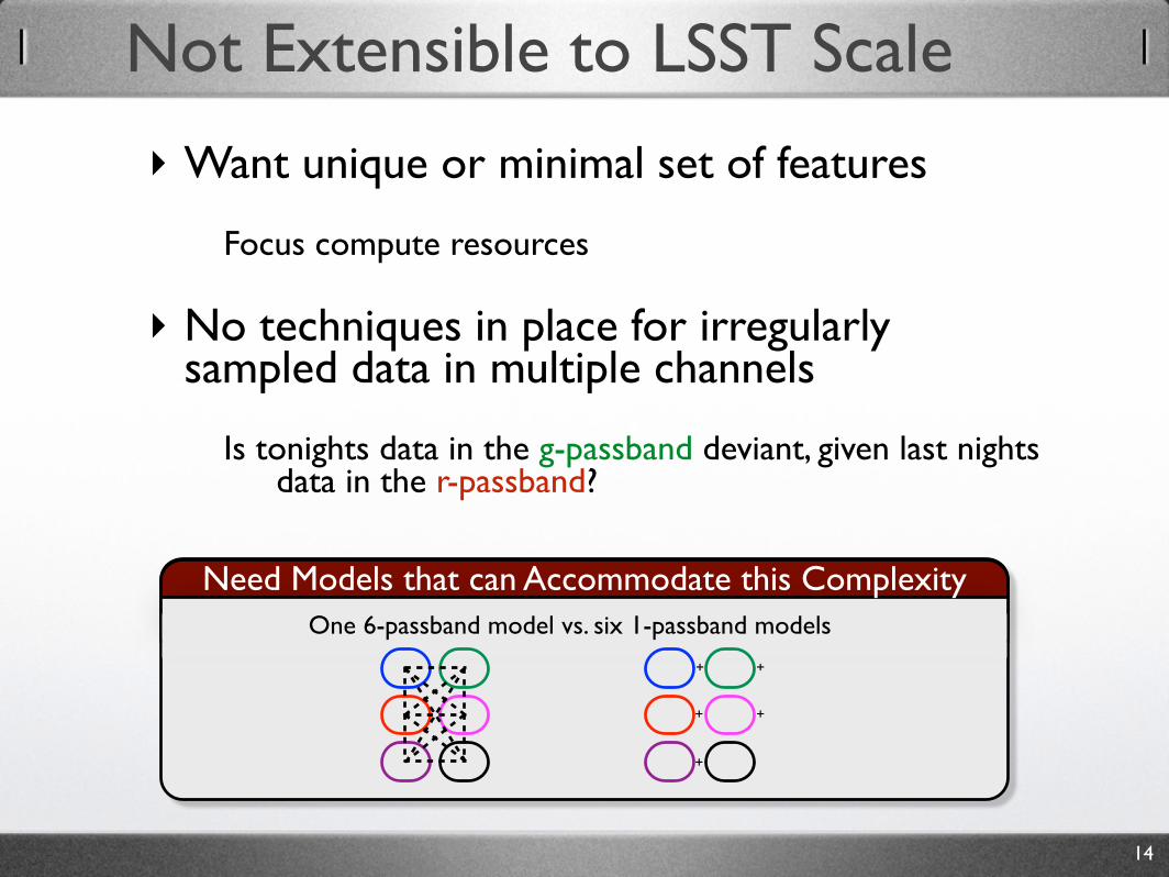
Not Extensible to LSST Scale
‣ Want unique or minimal set of features!
! ! Focus compute resources!
‣ No techniques in place for irregularly sampled data in multiple channels!
! ! Is tonights data in the g-passband deviant, given last nights ! ! ! data in the r-passband?
14
Need Models that can Accommodate this ComplexityOne 6-passband model vs. six 1-passband models
+ +
++
+
Challenges for Time-Series Modeling
‣ How quickly can you recognize the class of object!
‣ How quickly can you recognize the uniqueness of object!
‣ How quickly can you recognize when the object changes its behavior!
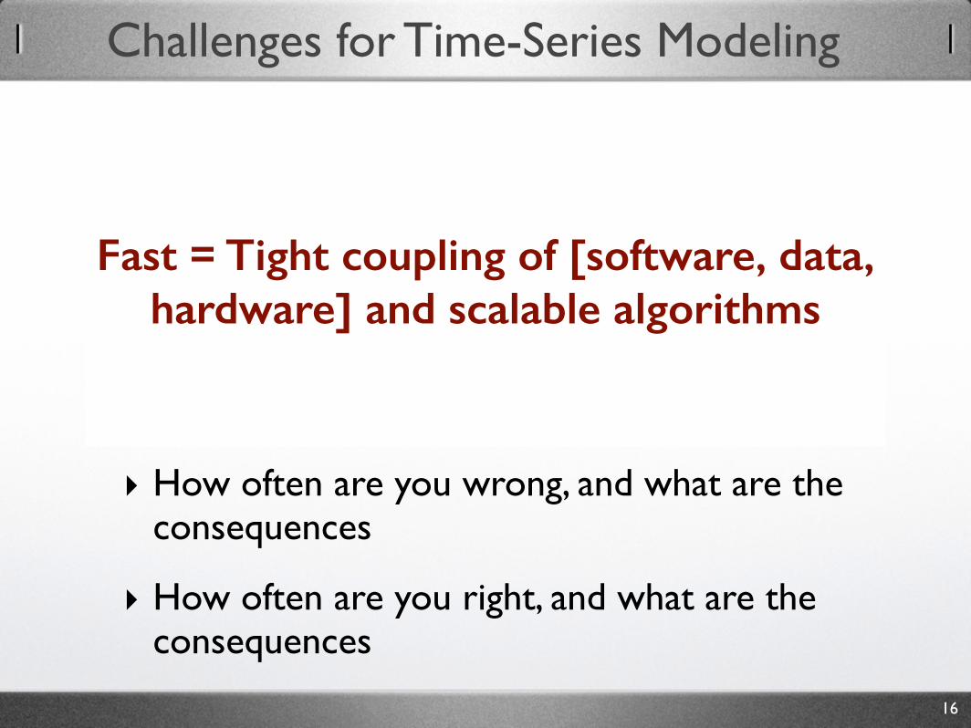
‣ How often are you wrong, and what are the consequences!
‣ How often are you right, and what are the consequences
15
Challenges for Time-Series Modeling
‣ How quickly can you recognize the class of object!
‣ How quickly can you recognize the uniqueness of object!
‣ How quickly can you recognize when the object changes its behavior!
‣ How often are you wrong, and what are the consequences!
‣ How often are you right, and what are the consequences
16
!
!
Fast = Tight coupling of [software, data, hardware] and scalable algorithms
!
Challenges for Time-Series Modeling
17
!
!
!
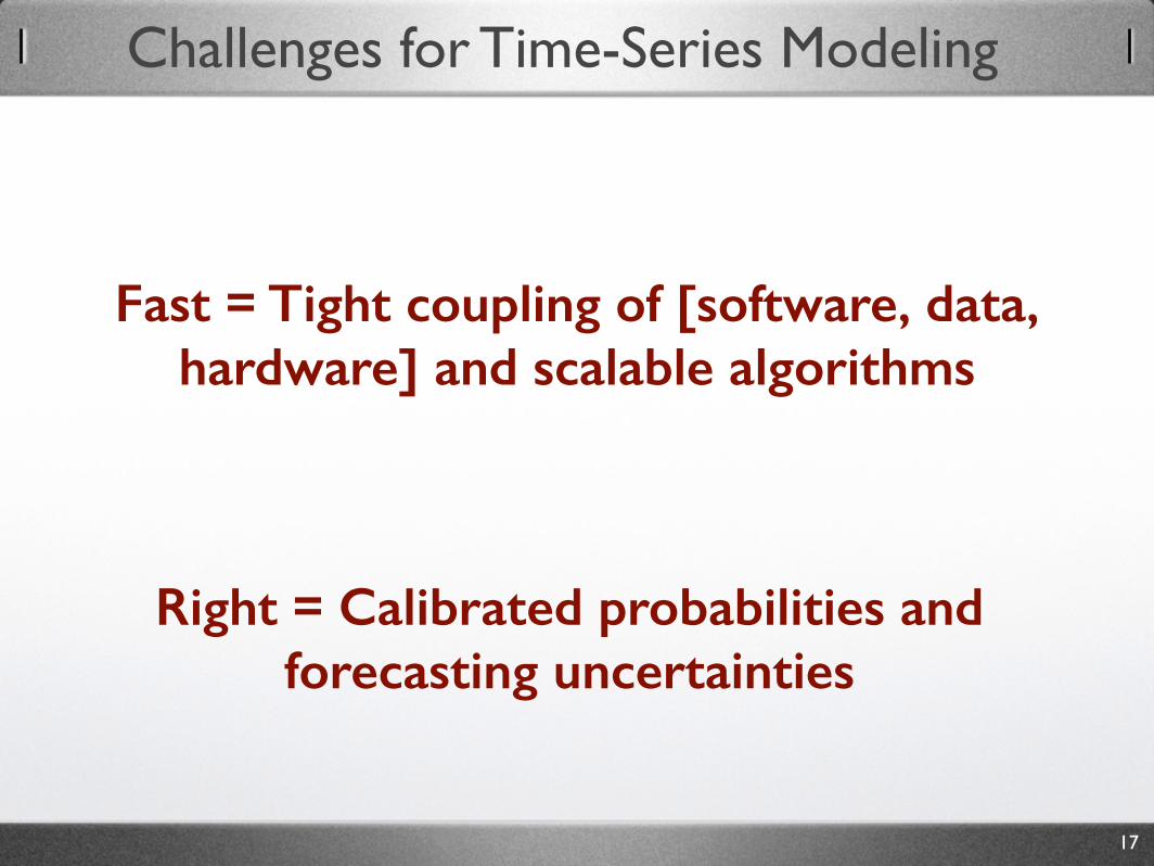
Right = Calibrated probabilities and forecasting uncertainties
!
!
!
Fast = Tight coupling of [software, data, hardware] and scalable algorithms
!
General Time-Series Models
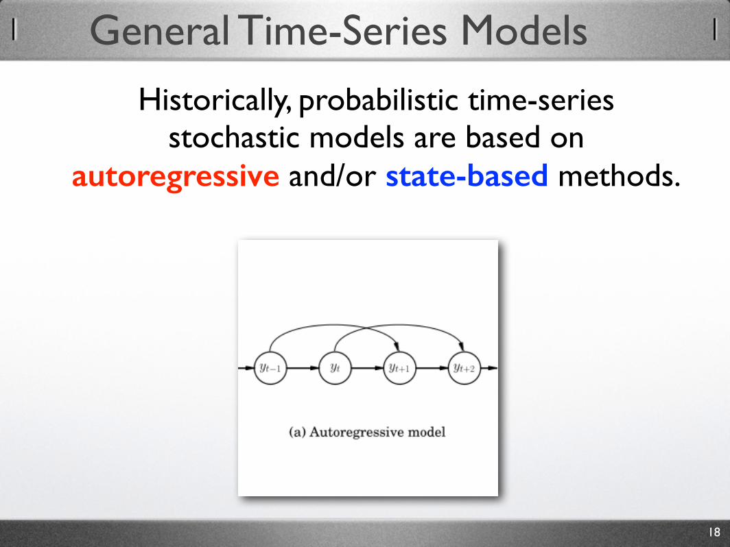
Historically, probabilistic time-series stochastic models are based on
autoregressive and/or state-based methods.
18

General Time-Series Models
Historically, probabilistic time-series stochastic models are based on
autoregressive and/or state-based methods.
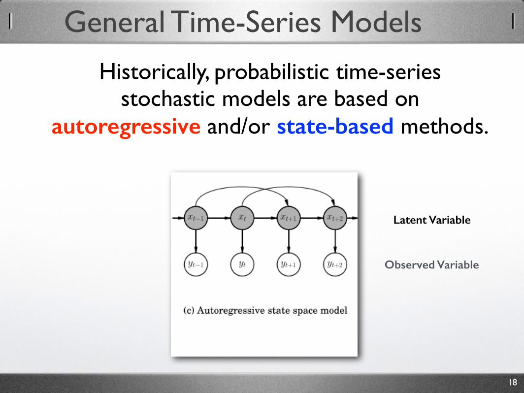
Latent Variable
Observed Variable
18
General Time-Series Models
Historically, probabilistic time-series stochastic models are based on
autoregressive and/or state-based methods.
Latent Variable
Observed Variable
18
CARMA Models
19
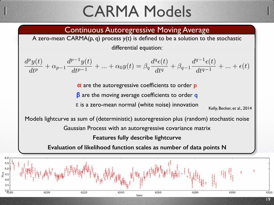
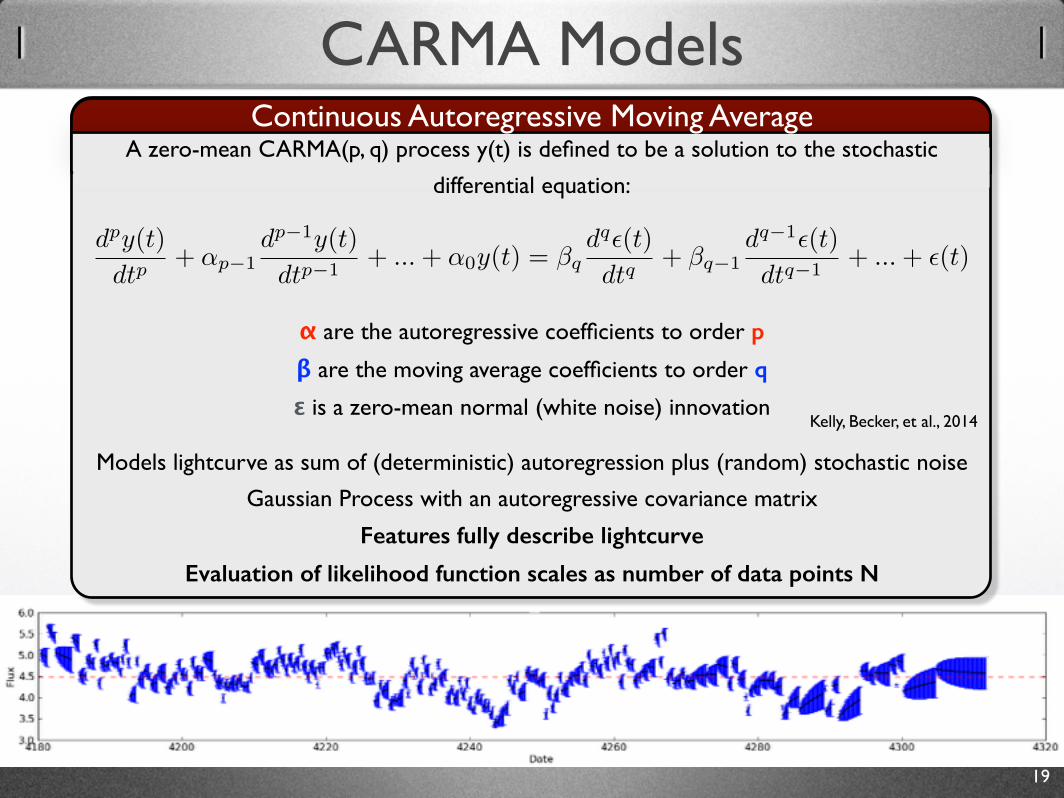
Continuous Autoregressive Moving AverageA zero-mean CARMA(p, q) process y(t) is defined to be a solution to the stochastic
differential equation:!
!!!
α are the autoregressive coefficients to order p!
β are the moving average coefficients to order q!
ε is a zero-mean normal (white noise) innovation
dpy(t)
dtp+ ↵p�1
dp�1y(t)
dtp�1+ ...+ ↵0y(t) = �q
dq✏(t)
dtq+ �q�1
dq�1✏(t)
dtq�1+ ...+ ✏(t)
Models lightcurve as sum of (deterministic) autoregression plus (random) stochastic noise!
Gaussian Process with an autoregressive covariance matrix!
Features fully describe lightcurve
Evaluation of likelihood function scales as number of data points N
Kelly, Becker, et al., 2014
CARMA Models
19
Continuous Autoregressive Moving AverageA zero-mean CARMA(p, q) process y(t) is defined to be a solution to the stochastic
differential equation:!
!!!
α are the autoregressive coefficients to order p!
β are the moving average coefficients to order q!
ε is a zero-mean normal (white noise) innovation
dpy(t)
dtp+ ↵p�1
dp�1y(t)
dtp�1+ ...+ ↵0y(t) = �q
dq✏(t)
dtq+ �q�1
dq�1✏(t)
dtq�1+ ...+ ✏(t)
Models lightcurve as sum of (deterministic) autoregression plus (random) stochastic noise!
Gaussian Process with an autoregressive covariance matrix!
Features fully describe lightcurve
Evaluation of likelihood function scales as number of data points N
Kelly, Becker, et al., 2014
Extending Models Using Bayesian Inference
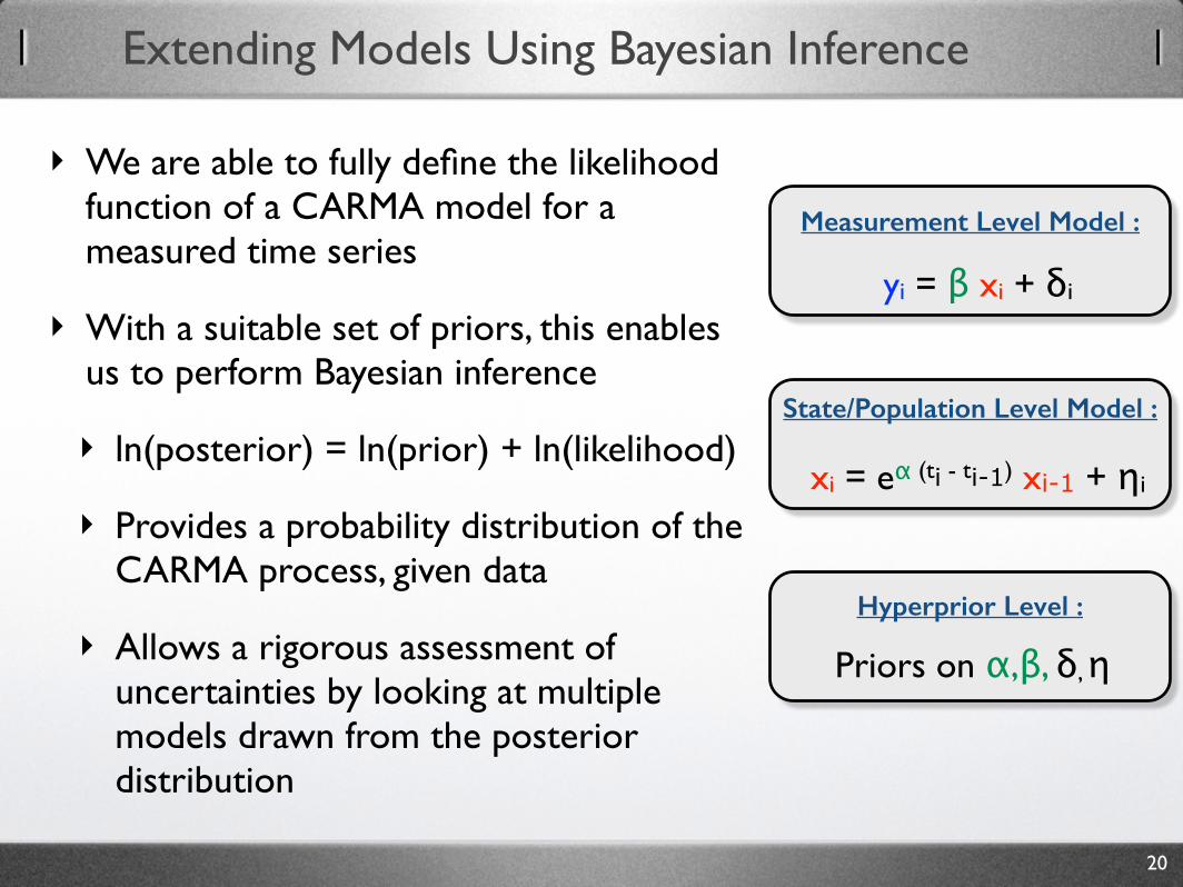
‣ We are able to fully define the likelihood function of a CARMA model for a measured time series!
‣ With a suitable set of priors, this enables us to perform Bayesian inference!
‣ ln(posterior) = ln(prior) + ln(likelihood)!
‣ Provides a probability distribution of the CARMA process, given data!
‣ Allows a rigorous assessment of uncertainties by looking at multiple models drawn from the posterior distribution
20
Measurement Level Model :
Priors on α,β, δ, η
xi = eα (ti - ti-1) xi-1 + ηi
yi = β xi + δi
State/Population Level Model :
Hyperprior Level :
Markov Chain Sampling of Posterior
21
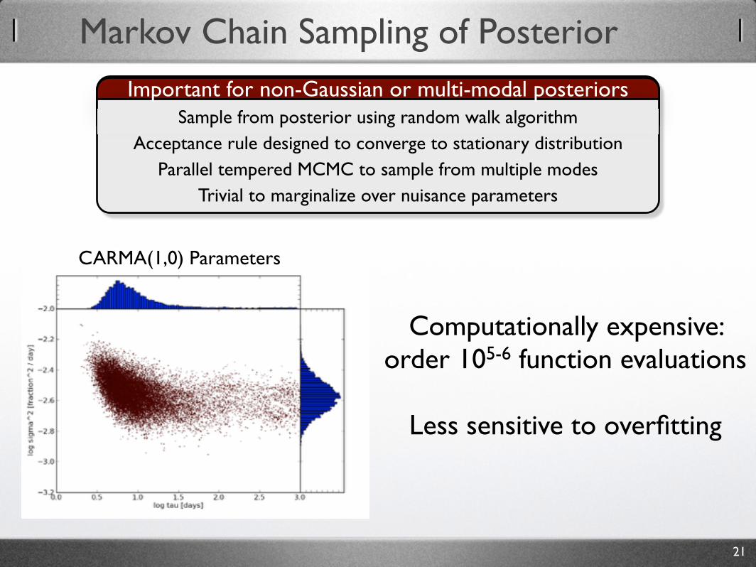
Important for non-Gaussian or multi-modal posteriorsSample from posterior using random walk algorithm!
Acceptance rule designed to converge to stationary distribution!Parallel tempered MCMC to sample from multiple modes!
Trivial to marginalize over nuisance parameters
CARMA(1,0) Parameters
Computationally expensive: order 105-6 function evaluations!
!Less sensitive to overfitting
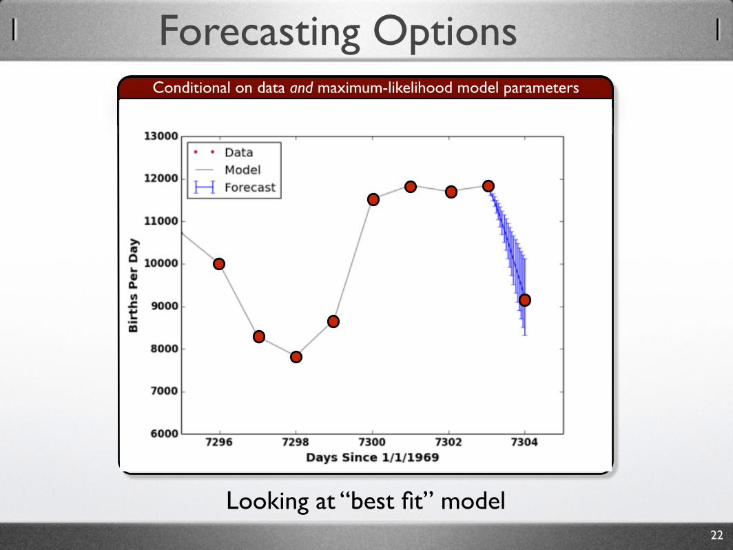
Forecasting Options
22
Conditional on data and MAP model Conditional on data and maximum-likelihood model parameters
Looking at “best fit” model
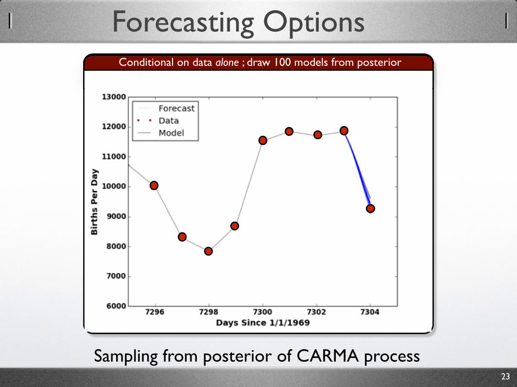
Forecasting Options
23
Conditional on data alone ; draw 100 models from posterior
Sampling from posterior of CARMA process
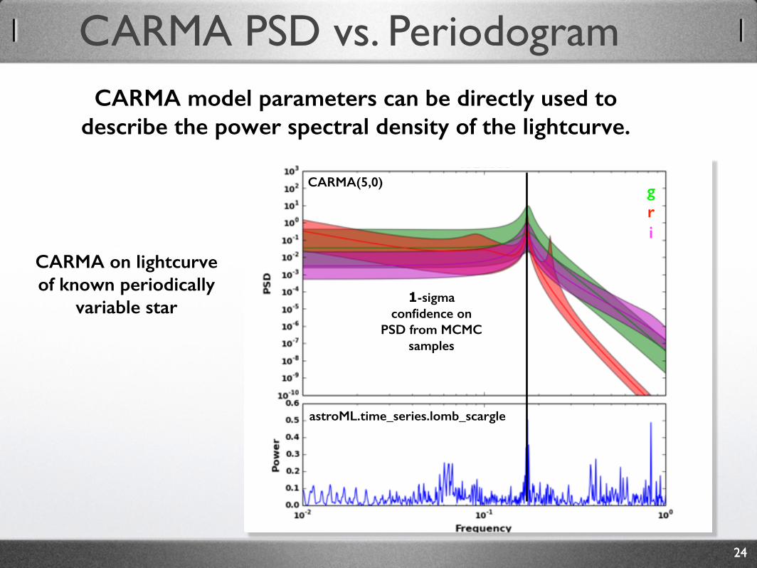
24
CARMA(5,0)
astroML.time_series.lomb_scargle
g r i
1-sigma confidence on
PSD from MCMC samples
24
CARMA PSD vs. Periodogram
CARMA on lightcurve of known periodically
variable star
CARMA model parameters can be directly used to describe the power spectral density of the lightcurve.
25
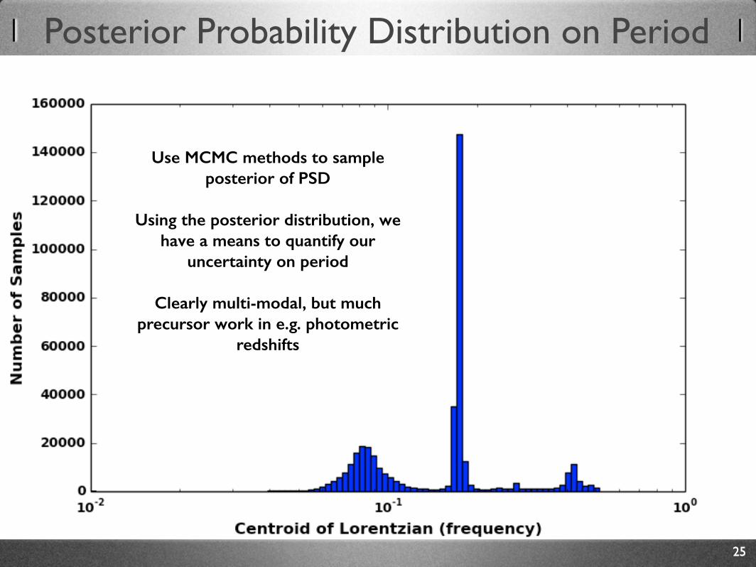
Posterior Probability Distribution on Period
25
Use MCMC methods to sample posterior of PSD
!Using the posterior distribution, we
have a means to quantify our uncertainty on period
!Clearly multi-modal, but much
precursor work in e.g. photometric redshifts
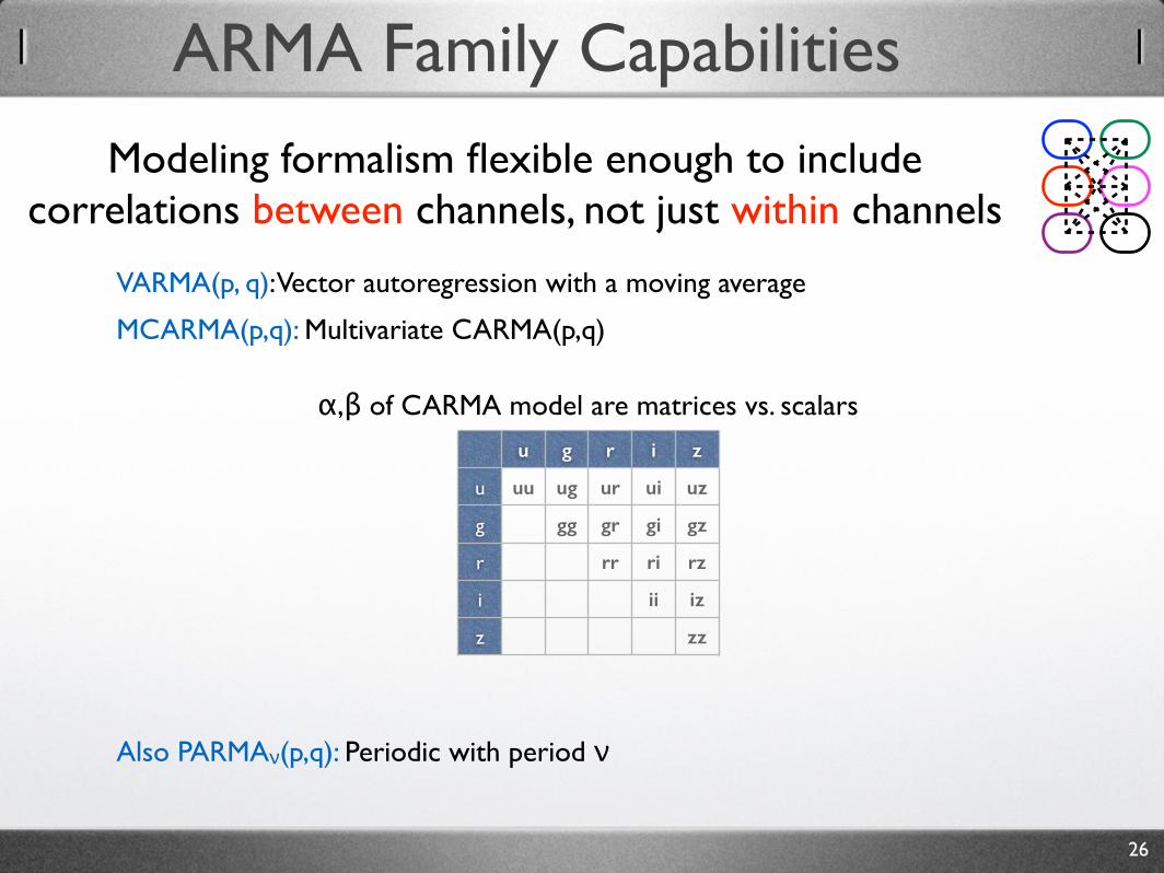
u g r i z
u uu ug ur ui uz
g gg gr gi gz
r rr ri rz
i ii iz
z zz
26
ARMA Family Capabilities
Modeling formalism flexible enough to include correlations between channels, not just within channels
VARMA(p, q): Vector autoregression with a moving average!
MCARMA(p,q): Multivariate CARMA(p,q)!
!!!!!!!!Also PARMAν(p,q): Periodic with period ν!
α,β of CARMA model are matrices vs. scalars
Single phenomenological model using all available data
27
ARMA Family Capabilities
Flexible through choice of autoregessive and moving average orders
Scalable through order(N) scaling of likelihood function, and online model update
Calibrated forecasting using Bayesian techniques
MCMC MCMC MCMCMCMC MCMC MCMC
MCMC MCMC MCMCMCMC MCMC MCMC
MCMC MCMC MCMCMCMC MCMC MCMC
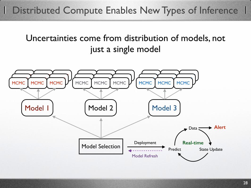
Distributed Compute Enables New Types of Inference
Uncertainties come from distribution of models, not just a single model
28
Model 1 Model 2 Model 3
MCMC MCMC MCMC MCMC MCMC MCMC MCMC MCMC MCMC
Model SelectionDeployment
Data
State UpdatePredict
Model Refresh
Real-time
Alert