fitting timeseries by continuous-time markov …eve2/tseries_jcp.pdffitting timeseries by...

Fitting timeseries by continuous-time Markov chains:A quadratic programming approach

D.T. Crommelin *, E. Vanden-Eijnden

Courant Institute of Mathematical Sciences, New York University, 251 Mercer Street, New York, NY 10012, USA

Received 5 October 2005; received in revised form 10 January 2006; accepted 23 January 2006Available online 15 March 2006

Abstract

Construction of stochastic models that describe the e!ective dynamics of observables of interest is an useful instrumentin various fields of application, such as physics, climate science, and finance. We present a new technique for the construc-tion of such models. From the timeseries of an observable, we construct a discrete-in-time Markov chain and calculate theeigenspectrum of its transition probability (or stochastic) matrix. As a next step we aim to find the generator of a contin-uous-time Markov chain whose eigenspectrum resembles the observed eigenspectrum as closely as possible, using anappropriate norm. The generator is found by solving a minimization problem: the norm is chosen such that the objectfunction is quadratic and convex, so that the minimization problem can be solved using quadratic programming tech-niques. The technique is illustrated on various toy problems as well as on datasets stemming from simulations of moleculardynamics and of atmospheric flows.! 2006 Elsevier Inc. All rights reserved.

PACS: 05.10.Gg; 02.50.Ga; 05.45.Tp; 36.20.Ey; 92.60.Bh; 02.30.Zz

MSC: 60J27; 60J22; 62M10; 62M05; 49N45

Keywords: Markov chains; Embedding problem; Inverse problems; Timeseries analysis

1. Introduction

Inverse modeling is a powerful tool for the investigation of complex systems in various fields of application.If models derived from first principles are either very complicated or just non-existing, inverse modeling –constructing models from available data – can be an interesting alternative. A typical situation where inversemodeling can be very useful is the case when a complex system yields relatively simple macroscopic behaviorthat may be captured with low-order models, but where the derivation of such low-order models from first prin-ciples is very di"cult or impossible. Such situations arise for example in molecular dynamics, econometrics,

0021-9991/$ - see front matter ! 2006 Elsevier Inc. All rights reserved.doi:10.1016/j.jcp.2006.01.045

* Corresponding author.E-mail addresses: [email protected] (D.T. Crommelin), [email protected] (E. Vanden-Eijnden).

Journal of Computational Physics 217 (2006) 782–805

www.elsevier.com/locate/jcp

mailto:[email protected]

mailto:[email protected]

or climate science. In this study we focus on the construction of low-order stochastic models in the form ofcontinuous-time Markov chains from timeseries.

To make things more precise and clarify the issues, let us start with a simpler problem. Consider a contin-uous-time Markov chain on a finite state-space S (for a general introduction to the theory of Markov chains,see [1,2]; continuous-time Markov chains are treated in detail in [3]). This chain is completely determined by itsgenerator L, that is, the matrix with nonnegative o!-diagonal elements, nonpositive diagonal elements andzero row sums (

PyL!x; y" # 0 8x 2 S) such that

limt!0$

Exf !X t" % f !x"t

#X

y2SL!x; y"f !y"; !1"

for all suitable test functions f : S ! R; here Ex denotes the expectation conditional on Xt=0 = x and Xt de-notes a sample path of the continuous-time Markov chain. Assume that the chain is ergodic and stationary,and denote by fX tgt2R the equilibrium trajectory of the chain in a given realization. Given a sampling of Xt atdiscrete time-intervals, fX tjgj2Z, with tj = jh, h > 0, how can we reconstruct the generator L of the chain? Sinceh is fixed and may be rather large, (1) cannot be used. Yet, one can define the transition probability matrix P(h)

whose elements P(h)(x,y) give the probability to have gone from state x to state y after a time-interval h:

P !h"!x; y" # limN!1

PNj#%N1!X jh # x"1!X !j$1"h # y"

PNj#%N1!X jh # x"

; !2"

where 1(Æ) denotes the indicator function, 1(Xjh = x) = 1 if Xjh = x and 1(Xjh = x) = 0 otherwise. By ergodicity,this limit exists and is unique, and P(h) and L are related as

P !h" # exp!hL"; L # h%1 log P !h". !3"

This relation o!ers a way to reconstruct L from P(h); log P(h) can be computed by using e.g. the spectraldecomposition of P(h) (see (7)).

Unfortunately, the above procedure is not practical for the actual problems that we want to address in thispaper in which:

(1) the discrete sampling is finite, i.e. we are only given fX tjgj#0;...;N corresponding to tj 2 [0,Nh] for someN < 1;

(2) the underlying process Xt may not be Markov since, in a typical application, Xt is the timeseries of anobservable which may display memory e!ects.

These features lead to the following practical di"culty. The matrix ~P !h" computed via

~P !h"!x; y" #PN%1

j#0 1!X jh # x"1!X !j$1"h # y"PN%1

j#0 1!X jh # x"; !4"

is, by construction, a stochastic matrix satisfyingP

y~P !h"!x; y" # 1 8x and ~P !h"!x; y" P 0 8x; y. However,

L # h%1 log ~P !h" will, in general, have some negative or even complex o!-diagonal elements and therefore willnot be acceptable since it is not a generator of a continuous-time Markov chain. This issue is in fact related tothe following famous (and open) embedding problem for Markov chains: not every discrete-in-time Markovchain (such as the one associated with ~P !h") has an underlying continuous-time chain, and the necessaryand su"cient conditions for this to be the case are unknown. It is known what conditions a matrix must satisfyin order to be a generator (real, nonnegative o!-diagonal elements; zero row sums); also, if L is a generatorthen all matrices P(h) = exp(hL) with h P 0 are stochastic matrices. However, it is not known what exact con-ditions a stochastic matrix Pmust satisfy so that it can be written as P = exp(hL) with L a generator and h P 0(i.e., the conditions for P to be embeddable). The subset of n · n embeddable matrices within the set of all n · nstochastic matrices has a very complicated geometrical structure (except if n = 2); in particular, it is non-con-vex. For more details on the embedding problem we refer to [4–7].

D.T. Crommelin, E. Vanden-Eijnden / Journal of Computational Physics 217 (2006) 782–805 783

The main result of this paper is an e"cient algorithm which gets around the di"culty posed by the embed-ding problem and permits to re-construct a true generator L from the observed ~P !h". This is done via the solu-tion of a variational problem: we find the generator L such that exp(hL) is the closest to the measuredstochastic matrix ~P !h" in the sense that their spectrum are the closest. If h%1 log!~P !h"" is a generator (i.e. if~P !h" is embeddable), then the procedure gives L # h%1 log!~P !h"". If h%1 log!~P !h"" is not a generator, then the pro-cedure gives the true generator L which is the closest to h%1 log!~P !h"" in the sense above. The resulting modelsgive a much more faithful representation of the statistics and dynamics of the given timeseries than modelsconstructed by only aiming to reproduce the equilibrium distribution and, possibly, a decorrelation time.Notice also that this construction is di!erent from other procedures that have been proposed in the literatureto go around the embedding problem. For instance, when a given P(h) does not have an exact underlying gen-erator because log(P(h)) has negative o!-diagonal elements, Israel et al. [6] propose to set the negative o!-diag-onal elements to zero and change the diagonal elements such that the condition of zero row sums is satisfied.The approximation method we describe in this paper is less ad hoc and, we believe, more attractive as itdirectly aims at reproducing key characteristics of the Markov chain like the leading modes of the eigenspec-trum of the measured ~P !h". Bladt and Sørensen [7] use maximum likelihood estimation to find a generatorgiven a timeseries. Their numerical procedure to find the maximum likelihood estimator seems e"cient butrather costly; moreover, the estimator may not exist in various cases. The latter problem becomes particularlyurgent if the sampling frequency is low (i.e., if h is large), or if the iterates of the estimator approach theboundary of the set of generators (which is likely to happen if the given data has no exact underlying gener-ator). These are circumstances that typically show up in applications; the approach we present here is capableof dealing with them.

The remainder of this paper is organized as follows: in Section 2 we recall the spectral decomposition ofa generator L (Section 2.1) and we give the variational problem used to determine the Markov chain gen-erator with an eigenspectrum that matches the observed spectrum as closely as possible (Section 2.2). Thisvariational problem involves the minimization of a quadratic object function subject to linear constraints,i.e. it leads to a quadratic programming problem, for which there are well-established solution methods. Theoverall numerical procedure and its cost are presented in Section 2.3, and some error estimates are given inSection 2.4. In Section 3, the algorithm is illustrated by using it to obtain approximate generators for toyproblems with and without exact underlying generators. In Sections 4 and 5, we apply the method to datafrom applications: one timeseries generated by a model simulating the dynamics of an alanine dipeptidemolecule in vacuum (Section 4), and another one obtained from a model that describes large-scale atmo-spheric flow (Section 5). In both case, the data are non-Markovian at short time-intervals; we show howto obtain good results by using information from longer time intervals. Concluding remarks and possiblegeneralizations are given in Section 6.

2. A quadratic programming approach

2.1. Preliminaries: spectral representation of the generator

Assume that the number of states in S is n, and let {wk,/k,kk}k=1, . . ., n with wk = (wk(1), . . .,wk(n)) and/k = (/k(1), . . .,/k(n))

T be the complete bi-orthogonal set of eigenmodes and eigenvalues of a generator L,

L/k # kk/k; wkL # kkwk; wk/l # dkl; !5"

ordered such that Rekk P Rekk+1 for all k. The first eigenmode (k = 1) has special properties, since it containsthe invariant distribution l(x) (assumed to be unique): w1 = l, /1 = (1, . . ., 1)T and k1 = 0. Assuming that alleigenvalues have multiplicity one, L can be represented as

L!x; y" #Xn

k#1

kk/k!x"wk!y". !6"

The spectral representation of L allows one to easily compute the exponential of L. Indeed, if P(h) = exp(hL),then P(h) can be represented as

784 D.T. Crommelin, E. Vanden-Eijnden / Journal of Computational Physics 217 (2006) 782–805

P !h"!x; y" #Xn

k#1

Kk/k!x"wk!y"; !7"

where Kk = exp(kkh). Conversely, if {wk,/k,Kk}k=1, . . ., n is the complete bi-orthogonal set of eigenmodes andeigenvalues of P(h) so that (7) holds, then L = h%1 logP(h) can be represented as in (6) with kk = h%1 logKk.

2.2. A quadratic variational problem

Suppose that we have constructed from (4) the stochastic matrix ~P !h" associated with the finite samplingfX tjgj#0;...;N , tj = jh, h > 0, N < 1. As explained in Section 1, the stochastic matrix ~P !h" may have no true gen-erator associated with it. This means that if f~wk; ~/k; ~Kkg is the complete bi-orthogonal set of eigenmodes andeigenvalues of ~P !h" so that ~P !h" can be represented as

~P !h"!x; y" #Xn

k#1

~Kk~/k!x"~wk!y"; !8"

the matrix

~L!x; y" #Xn

k#1

~kk ~/k!x"~wk!y" where ~kk # h%1 log ~Kk !9"

will in general have negative or even complex o!-diagonal element and will therefore not qualify as a generatorof a continuous-time Markov chain.

To get around this di"culty, we propose to find a true generator L(x,y) optimal with respect to the data athand by minimizing the following object function under variation of L:

E #Xn

k#1

akj~wkL% ~kk ~wkj2 $ bkjL~/k % ~kk ~/kj2 $ ckj~wkL~/k % ~kkj2! "

!10"

subject to the constraints

L!x; x" # %X

y2Sy 6#x

L!x; y" 8x 2 S !11"

and

L!x; y" P 0 8x; y 2 S with x 6# y. !12"

In (10) ak, bk, ck are weights, typically of the form ak # ~akj~kk ~wkj%2, bk # ~bkj~kk ~/kj%2, ck # ~ckj~kkj%2. If we thenpick ~ak # ~bk # ~ck # 1 8k, relative errors of the same order in the eigenvectors and eigenvalues of L will givecontributions of similar magnitude in E.

The constraint (11) can be straightforwardly accounted for explicitly in (10), and one is then left with a qua-dratic functional which can be compactly written as:

E!L" # 1

2hL;HLi$ hF ; Li$ E0. !13"

Here

hL;HLi #X

x;y;x0 ;y02Sx6#y;x0 6#y0

L!x; y"H!x; y; x0; y0"L!x0; y 0";

hF ; Li #X

x;y2Sx6#y

F !x; y"L!x; y"!14"

and we defined


H!x; y; x0; y 0" #2Xn

k#1

!ak!d!x; x0" $ d!y; y0" % d!x0; y" % d!x; y0""~wk!x"!~wk!x0"

$ bkd!x; x0"!~/k!x" % ~/k!y""!!~/k!x0" % !~/k!y 0"" $ ck ~wk!x"!~wk!x0"!!~/k!x0" % !~/k!y0"""; !15"

F !x; y" #Xn

k#1

!ak~kk!~wk!x"!~wk!x" % ~wk!y"!~wk!x"" $ bk~kk/k!x"!!/k!x" % !/k!y"" $ ck~kk

!~wk!x"!!~/k!x" % !~/k!y""

$ complex conjugate"; !16"

E0 #Xn

k#1

~kk!~kk

X

x

!ak ~wk!x"!~wk!x" $ bk~/k!x"!~/k!x" $ ck

!

; !17"

where the bar denotes complex conjugate. (13) is a quadratic object function to be minimized over all L(x,y)with x; y 2 S and x 6# y subject to (12). Since there are n2 % n o!-diagonal elements in L, E should be thought

of as a function on Rn2%n. E is also convex since it is straightforward to check that the level sets of E are ellip-soids in Rn2%n centered around the point in Rn2%n associated with the o!-diagonal elements of ~L given in (9).Thus ~L is the absolute minimizer of (13) with E!~L" # 0. ~L is also the minimizer of (13) subject to (12) if ~P !h" isembeddable, since in this case ~L satisfies (12). If ~P !h" is not embeddable, ~L is not the minimum of E subject to(12), but the minimization problem still has a unique solution because because the domain for L defined by(12) is a convex domain in Rn2%n. The corresponding minimizer Lmin is the unique true generator ‘‘closest’’to ~L.

One can use other object functions than (10) to formulate the search for an optimal generator as a mini-mization problem. In particular, it is easy to show that the minimizer of

E0 #X

x;y2Sx6#y

jL!x; y" % ~L!x; y"j2; !18"

over all matrices L such that L(x,y) P 0 if x 6# y must be

L!x; y" # max!Re~L!x; y"; 0" if x 6# y; !19"

which can be supplemented by L!x; x" # %P

y 6#xL!x; y" to obtain a generator. The disadvantage of using (18),however, is that the information on the eigenvectors and eigenvalues of ~L enters only very indirectly (18),which means that the spectrum of (19) may be rather di!erent from those of ~L. In contrast, (10) preciselyaim at reproducing the spectrum of ~L as closely as possible, which is important since this spectrum embedsthe most important features of the dynamics of Xt.

2.3. Numerical procedure and computational cost

The minimization of (13) subject to (12) defines a standard quadratic problem which can be solved via well-established numerical methods (see e.g. [8,9]). For this study we use the internal quadratic programming algo-rithm of Matlab; various other software packages are also available to solve this type of problems. As inputfor the Matlab algorithm the matrix H and the vectors F are needed, as well as an initial guess for L.

As mentioned earlier, for a Markov chain with n states, the minimization problem is of dimension n2 % nand has n2 % n inequality constraints, see (12). The computational cost of a quadratic programming algorithmmay become prohibitive when the number of states in the chain is large. One particularly interesting way toreduce the size of the minimization problem, and thereby the computational cost, is to restrict the class ofallowed Markov chain generators. For example, when considering a certain system there may be physicalgrounds for allowing only non-zero transition rates from one state to a selected few other states. This willbe the case e.g. if the state-space S inherits some topology from the physical space where the actual dynamicstakes place (as will be the case in the examples treated in Sections 4 and 5). If for instance, each state isconnected to m < n other states only, yielding a mn-dimensional minimization problem. We will discuss thispossibility in more detail in Section 6.


2.4. Error estimates

The computational strategy that we propose has two sources of errors as far as the fitting of the observedtimeseries by the continuous-time Markov chain is concerned. The first stems from the fact that the timeseriesmay not be Markov. In this case, the Markov assumption itself is a source of error. This error may dominatein many applications, but it is hard to quantify systematically. Therefore, we shall not dwell on this issue inthis section and postpone its discussion till Sections 4 and 5 where we investigate it via numerical experimentsand show how our computational strategy allows to overcome errors due to non-Markovianity of thetimeseries.

The second source of error is that, even if the observed timeseries is Markov and the exact matrix P(h) givenby (2) is embeddable, in general ~P !h" 6# P !h" due to finite sampling. As a result the observed spectrum will bedi!erent from the actual spectrum of the chain. This is the error that we quantify in this section.

2.4.1. Central limit theorem and error estimate on ~L # h%1 log ~P !h"

Let P(h) = exp(hL) be the true transition probability matrix underlying the timeseries from which we haveconstructed ~P !h" according to (4). Assume that the chain has been sampled at N = ºT/hß successive pointswith uniform time interval h, consistent with the process being observed on a fixed window of timeT > 0 independent of the lag h. The error on ~P !h" obeys a version of the central limit theorem, see [10]:as T ! 1,

####T

p!~P !h" % P !h"" !

###h

pQ!h"; !20"

in probability, where Q(h) is a Gaussian matrix with mean zero and covariance

EQ!h"!x; y"Q!h"!x0; y0" # P !h"!x; y"l!x"

!d!y; y 0" % P !h"!x; y0""d!x; x0". !21"

For ~L # h%1 log ~P !h" we have

~L% L # h%1 log&1$ !P !h""%1!~P !h" % P !h""' ( h%1!P !h""%1!~P !h" % P !h"" !22"

since ~P !h" ( P !h" as T becomes large. This implies that as T ! 1,

####T

p!~L% L" ! 1###

hp !P !h""%1Q!h"; !23"

where we have used (20), and Q(h) is the same matrix as above.

2.4.2. Error estimates on the eigenspectrumUsing standard matrix perturbation theory one can use (20) to derive the following convergence estimates

on the eigenspectrum f~wk; ~/k; ~kkg of ~L # h%1 log ~P !h": as T ! 1,####T

p!~kk % kk" ! 1##

hp e%kkhwkQ

!h"/k;####T

p!~wk % wk" !

###h

pwkR

!h"k Q!h";

####T

p!~/k % /k" !

###h

pR!h"k Q!h"/k

8>><

>>:!24"

in probability. Here {wk,/k,kk} is the set of eigenvectors and eigenvalues of L, Q(h) is the Gaussian matrixdefined before, and

R!h"k !x; y" #

X

q6#k

!ekkh % ekqh"%1/q!x"wq!y".

For k = 1 a stronger estimate can be derived, since by construction ~k1 # 0 and ~/1 # !1; . . . ; 1"T (i.e., the errorson ~k1 and ~/1 are always zero). For ~w1 we have, as T ! 1,

####T

p!~w1 % l" !

###h

pb!h" !25"

in probability, where b(h) is a Gaussian vector with mean zero and covariance


Eb!h"!x"b!h"!y" # l!x"!d!x; y" % l!y"" $X

q6#1

ekqh

1% ekqh!wq!x"/q!y"l!y" $ wq!y"/q!x"l!x"". !26"

3. Toy examples

3.1. A toy example with exact generator

As a first test, we generate a timeseries for a simple 4-state Markov chain that has an exact underlyinggenerator, and use the timeseries to reconstruct the generator. This allows us to assess the convergence ofthe algorithm with the length of the timeseries. We choose the true generator to be

Lexact #

%0:6 0:4 0:2 0

0:5 %1:2 0:4 0:3

0:3 0 %0:6 0:3

0 0:1 0:2 %0:3

0

BBB@

1

CCCA. !27"

A sample path is generated from this generator and sampled at timelag h = 1. The eigenvalues of Lexact are 0,%0.40, %0.89, %1.42, so h = 1 is of the order of the characteristic timescale of the system. We use timeserieswith 10n data points, with n = 3, . . ., 7. Thus, the stochastic matrix ~P is calculated from 10n data points, and theeigenspectrum of ~P is used in the object function (10). For all calculations, the object function coe"cients areset to ~ak # ~bk # ~ck # 1 for all k = 1,2,3,4.

The generators obtained by minimizing (10) subject to (12) are denoted by L10n

min; the generators constructedfrom the same 10n data points according to (9) are denoted by ~L10n . From the ~L10n we also construct ~L10n

g using(19). Thus the L10n

min and ~L10n

g always are true generator, whereas the ~L10n may not (they usually have one or morenegative o!-diagonal elements).

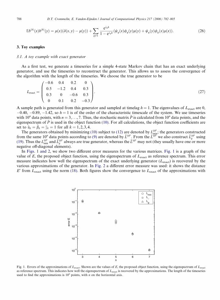
In Figs. 1 and 2, we show two di!erent error measures for the various matrices. Fig. 1 is a graph of thevalue of E, the proposed object function, using the eigenspectrum of Lexact as reference spectrum. This errormeasure indicates how well the eigenspectrum of the exact underlying generator (Lexact) is recovered by thevarious approximations of the generator. In Fig. 2 a di!erent error measure was used: it shows the distanceE 0 from Lexact using the norm (18). Both figures show the convergence to Lexact of the approximations with

3 4 5 6 7

10–5

10–4

10–3

10–2

10–1

100

n

erro

r E

Lmin

L~

Lg

Fig. 1. Errors of the approximations of Lexact. Shown are the values of E, the proposed object function, using the eigenspectrum of Lexact

as reference spectrum. This indicates how well the eigenspectrum of Lexact is recovered by the approximations. The length of the timeseriesused to find the approximations is 10n points, with n on the horizontal axis.


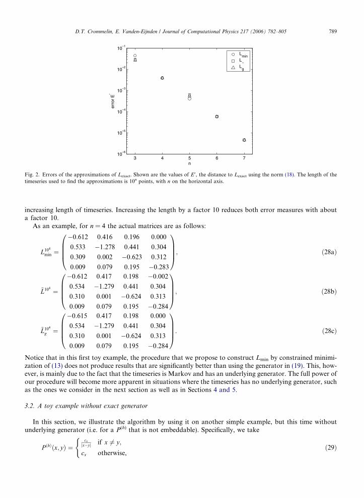
increasing length of timeseries. Increasing the length by a factor 10 reduces both error measures with abouta factor 10.

As an example, for n = 4 the actual matrices are as follows:

L104

min #

%0:612 0:416 0:196 0:000

0:533 %1:278 0:441 0:304

0:309 0:002 %0:623 0:312

0:009 0:079 0:195 %0:283

0

BBB@

1

CCCA; !28a"

~L104 #

%0:612 0:417 0:198 %0:002

0:534 %1:279 0:441 0:304

0:310 0:001 %0:624 0:313

0:009 0:079 0:195 %0:284

0

BBB@

1

CCCA; !28b"

~L104

g #

%0:615 0:417 0:198 0:000

0:534 %1:279 0:441 0:304

0:310 0:001 %0:624 0:313

0:009 0:079 0:195 %0:284

0

BBB@

1

CCCA. !28c"

Notice that in this first toy example, the procedure that we propose to construct Lmin by constrained minimi-zation of (13) does not produce results that are significantly better than using the generator in (19). This, how-ever, is mainly due to the fact that the timeseries is Markov and has an underlying generator. The full power ofour procedure will become more apparent in situations where the timeseries has no underlying generator, suchas the ones we consider in the next section as well as in Sections 4 and 5.

3.2. A toy example without exact generator

In this section, we illustrate the algorithm by using it on another simple example, but this time withoutunderlying generator (i.e. for a P(h) that is not embeddable). Specifically, we take

P !h"!x; y" #cx

jx%yj if x 6# y;

cx otherwise,

(

!29"

3 4 5 6 710

–6

10–5

10–4

10–3

10–2

10–1

n

erro

r E

!

Lmin

L~

Lg

Fig. 2. Errors of the approximations of Lexact. Shown are the values of E 0, the distance to Lexact using the norm (18). The length of thetimeseries used to find the approximations is 10n points, with n on the horizontal axis.


where the cx are normalization constants such thatP

yP!h"!x; y" # 1 8x (thereby ensuring that P(h) is a stochas-

tic matrix). We choose the state-space to have 10 states: x,y 2 {1,2, . . ., 10}. The value of the lag h is irrelevanthere; we set it to 1 (taking another value would only correspond to a time rescaling of the Markov chain). Theeigenvalues ~Kk of P

(h) are all real; four are on the negative real axis. Therefore, P(h) has no exact underlyinggenerator. For the reference eigenvalues ~kk we take log j~Kkj if ~Kk is negative and real; log ~Kk otherwise.

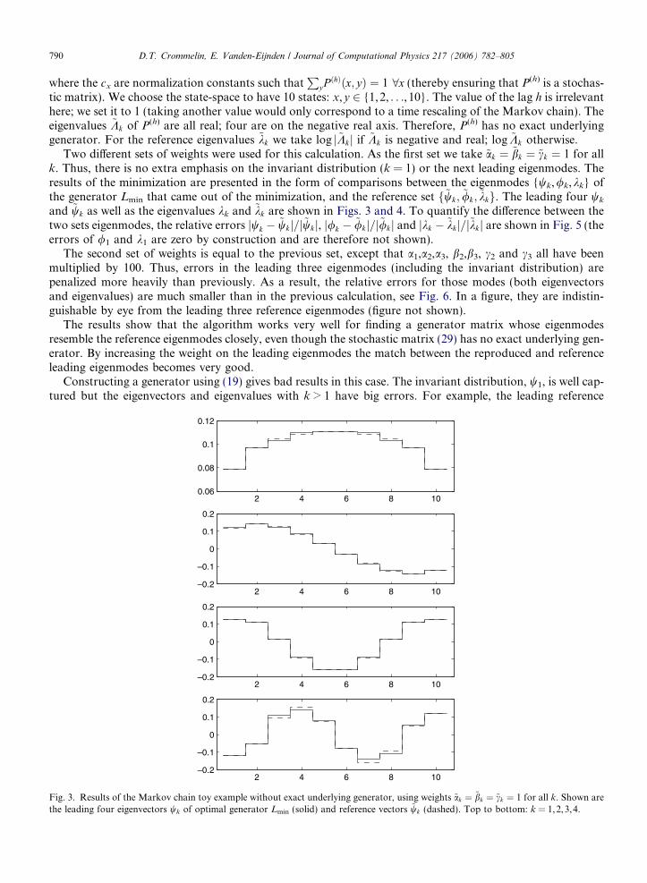
Two di!erent sets of weights were used for this calculation. As the first set we take ~ak # ~bk # ~ck # 1 for allk. Thus, there is no extra emphasis on the invariant distribution (k = 1) or the next leading eigenmodes. Theresults of the minimization are presented in the form of comparisons between the eigenmodes {wk,/k,kk} ofthe generator Lmin that came out of the minimization, and the reference set f~wk; ~/k; ~kkg. The leading four wk

and ~wk as well as the eigenvalues kk and ~kk are shown in Figs. 3 and 4. To quantify the di!erence between thetwo sets eigenmodes, the relative errors jwk % ~wkj=j~wkj, j/k % ~/kj=j~/kj and jkk % ~kkj=j~kkj are shown in Fig. 5 (theerrors of /1 and k1 are zero by construction and are therefore not shown).

The second set of weights is equal to the previous set, except that a1,a2,a3, b2,b3, c2 and c3 all have beenmultiplied by 100. Thus, errors in the leading three eigenmodes (including the invariant distribution) arepenalized more heavily than previously. As a result, the relative errors for those modes (both eigenvectorsand eigenvalues) are much smaller than in the previous calculation, see Fig. 6. In a figure, they are indistin-guishable by eye from the leading three reference eigenmodes (figure not shown).

The results show that the algorithm works very well for finding a generator matrix whose eigenmodesresemble the reference eigenmodes closely, even though the stochastic matrix (29) has no exact underlying gen-erator. By increasing the weight on the leading eigenmodes the match between the reproduced and referenceleading eigenmodes becomes very good.

Constructing a generator using (19) gives bad results in this case. The invariant distribution, w1, is well cap-tured but the eigenvectors and eigenvalues with k > 1 have big errors. For example, the leading reference

2 4 6 8 100.06

0.08

0.1

0.12

2 4 6 8 10–0.2

–0.1

0

0.1

0.2

2 4 6 8 10–0.2

–0.1

0

0.1

0.2

2 4 6 8 10–0.2

–0.1

0

0.1

0.2

Fig. 3. Results of the Markov chain toy example without exact underlying generator, using weights ~ak # ~bk # ~ck # 1 for all k. Shown arethe leading four eigenvectors wk of optimal generator Lmin (solid) and reference vectors ~wk (dashed). Top to bottom: k = 1,2,3,4.


2 4 6 8 10

100

101

k

Eig

enva

lue

(x–1

)

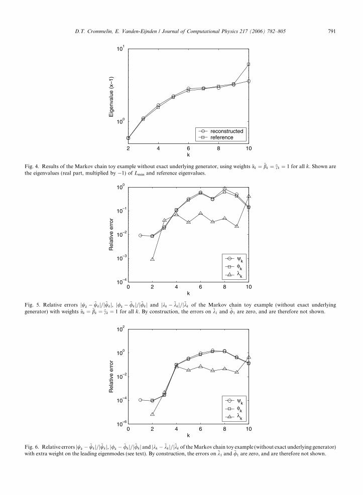
reconstructedreference

Fig. 4. Results of the Markov chain toy example without exact underlying generator, using weights ~ak # ~bk # ~ck # 1 for all k. Shown arethe eigenvalues (real part, multiplied by %1) of Lmin and reference eigenvalues.

0 2 4 6 8 1010

–4

10–3

10–2

10–1

100

k

Rel

ativ

e er

ror

"k

#k

$k

Fig. 5. Relative errors jwk % ~wk j=j~wk j, j/k % ~/k j=j~/k j and jkk % ~kk j=j~kk of the Markov chain toy example (without exact underlyinggenerator) with weights ~ak # ~bk # ~ck # 1 for all k. By construction, the errors on ~k1 and ~/1 are zero, and are therefore not shown.

0 2 4 6 8 1010

–6

10–4

10–2

100

102

k

Rel

ativ

e er

ror

"k

#k

$k

Fig. 6. Relative errors jwk % ~wk j=j~wk j, j/k % ~/k j=j~/k j and jkk % ~kk j=j~kk of theMarkov chain toy example (without exact underlying generator)with extra weight on the leading eigenmodes (see text). By construction, the errors on ~k1 and ~/1 are zero, and are therefore not shown.


eigenvalues are ~k2 # %0:60; ~k3 # %1:08; the generator obtained from (19) gives k2 = %1.53, k3 = %2.37. Bycontrast, the generator obtained with our proposed object function has relative errors for k2 and k3 of about10%2 using the first set of weights (Fig. 5) and about 10%4 using the second set of weights (Fig. 6).

4. Application to a timeseries from molecular dynamics

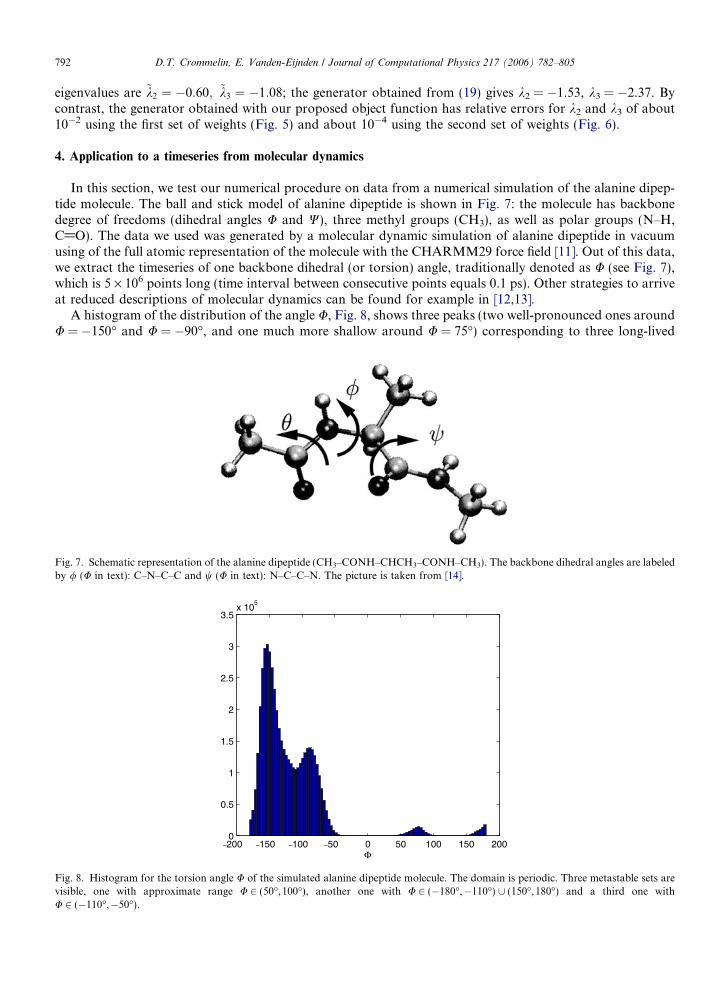
In this section, we test our numerical procedure on data from a numerical simulation of the alanine dipep-tide molecule. The ball and stick model of alanine dipeptide is shown in Fig. 7: the molecule has backbonedegree of freedoms (dihedral angles U and W), three methyl groups (CH3), as well as polar groups (N–H,C@O). The data we used was generated by a molecular dynamic simulation of alanine dipeptide in vacuumusing of the full atomic representation of the molecule with the CHARMM29 force field [11]. Out of this data,we extract the timeseries of one backbone dihedral (or torsion) angle, traditionally denoted as U (see Fig. 7),which is 5 · 106 points long (time interval between consecutive points equals 0.1 ps). Other strategies to arriveat reduced descriptions of molecular dynamics can be found for example in [12,13].

A histogram of the distribution of the angle U, Fig. 8, shows three peaks (two well-pronounced ones aroundU = %150" and U = %90", and one much more shallow around U = 75") corresponding to three long-lived

Fig. 7. Schematic representation of the alanine dipeptide (CH3–CONH–CHCH3–CONH–CH3). The backbone dihedral angles are labeledby / (U in text): C–N–C–C and w (U in text): N–C–C–N. The picture is taken from [14].

–200 –150 –100 –50 0 50 100 150 2000

0.5

1

1.5

2

2.5

3

3.5x 10

5

%

Fig. 8. Histogram for the torsion angle U of the simulated alanine dipeptide molecule. The domain is periodic. Three metastable sets arevisible, one with approximate range U 2 (50",100"), another one with U 2 (%180",%110") [ (150", 180") and a third one withU 2 (%110",%50").


conformation states that characterize alanine dipeptide (see e.g. [15,14,16]). Since the three sets can be distin-guished in the histogram of U, we want to find a generator that correctly describes the statistics and dynamicsof U alone. This is a particularly di"cult test, since typically both torsion angles U and W are used in attemptsto find a reduced description of the macrostate dynamics of the molecule (as, for instance, in [13]). We bin thedata (i.e. U) into 10 bins of 36" each, thereby obtaining a state space S with 10 states. The timeseries is binnedaccordingly.

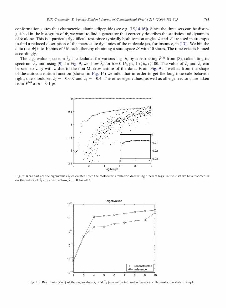
The eigenvalue spectrum ~kk is calculated for various lags h, by constructing ~P !h" from (8), calculating itsspectrum ~Kk and using (9). In Fig. 9, we show ~kk for h = 0.1hn ps, 1 6 hn 6 100. The value of ~k2 and ~k3 canbe seen to vary with h due to the non-Markov nature of the data. From Fig. 9 as well as from the shapeof the autocorrelation function (shown in Fig. 14) we infer that in order to get the long timescale behaviorright, one should set ~k2 # %0:007 and ~k3 # %0:4. The other eigenvalues, as well as all eigenvectors, are takenfrom P(h) at h = 0.1 ps.

0 2 4 6 8 10–2.5

–2

–1.5

–1

–0.5

0

lag h in ps

0 5 10–0.03

–0.02

–0.01

0

Fig. 9. Real parts of the eigenvalues ~kk calculated from the molecular simulation data using di!erent lags. In the inset we have zoomed inon the values of ~k2 (by construction, ~k1 # 0 for all h).

2 3 4 5 6 7 8 9 1010

–3

10–2

10–1

100

101

102

eigenvalues


Fig. 10. Real parts (·%1) of the eigenvalues kk and ~kk (reconstructed and reference) of the molecular data example.


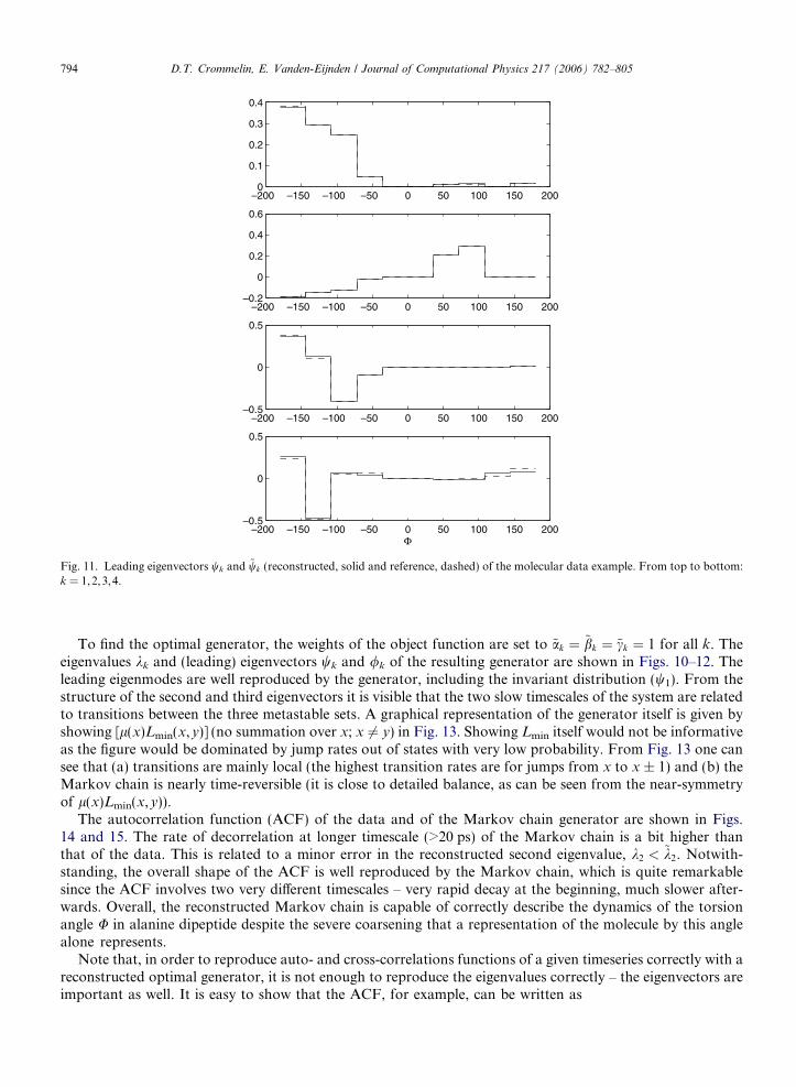
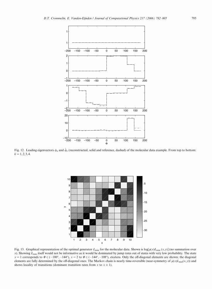
To find the optimal generator, the weights of the object function are set to ~ak # ~bk # ~ck # 1 for all k. Theeigenvalues kk and (leading) eigenvectors wk and /k of the resulting generator are shown in Figs. 10–12. Theleading eigenmodes are well reproduced by the generator, including the invariant distribution (w1). From thestructure of the second and third eigenvectors it is visible that the two slow timescales of the system are relatedto transitions between the three metastable sets. A graphical representation of the generator itself is given byshowing [l(x)Lmin(x,y)] (no summation over x; x 6# y) in Fig. 13. Showing Lmin itself would not be informativeas the figure would be dominated by jump rates out of states with very low probability. From Fig. 13 one cansee that (a) transitions are mainly local (the highest transition rates are for jumps from x to x ± 1) and (b) theMarkov chain is nearly time-reversible (it is close to detailed balance, as can be seen from the near-symmetryof l(x)Lmin(x,y)).

The autocorrelation function (ACF) of the data and of the Markov chain generator are shown in Figs.14 and 15. The rate of decorrelation at longer timescale (>20 ps) of the Markov chain is a bit higher thanthat of the data. This is related to a minor error in the reconstructed second eigenvalue, k2 < ~k2. Notwith-standing, the overall shape of the ACF is well reproduced by the Markov chain, which is quite remarkablesince the ACF involves two very di!erent timescales – very rapid decay at the beginning, much slower after-wards. Overall, the reconstructed Markov chain is capable of correctly describe the dynamics of the torsionangle U in alanine dipeptide despite the severe coarsening that a representation of the molecule by this anglealone represents.

Note that, in order to reproduce auto- and cross-correlations functions of a given timeseries correctly with areconstructed optimal generator, it is not enough to reproduce the eigenvalues correctly – the eigenvectors areimportant as well. It is easy to show that the ACF, for example, can be written as

–200 –150 –100 –50 0 50 100 150 2000

0.1

0.2

0.3

0.4

–200 –150 –100 –50 0 50 100 150 200–0.2

0

0.2

0.4

0.6

–200 –150 –100 –50 0 50 100 150 200–0.5

0

0.5

–200 –150 –100 –50 0 50 100 150 200–0.5

0

0.5

%

Fig. 11. Leading eigenvectors wk and ~wk (reconstructed, solid and reference, dashed) of the molecular data example. From top to bottom:k = 1,2,3,4.


–200 –150 –100 –50 0 50 100 150 200

1

1

–200 –150 –100 –50 0 50 100 150 200–1

0

1

2

–200 –150 –100 –50 0 50 100 150 200–2

–1

0

1

–200 –150 –100 –50 0 50 100 150 200–10

0

10

20

%

Fig. 12. Leading eigenvectors /k and ~/k (reconstructed, solid and reference, dashed) of the molecular data example. From top to bottom:k = 1,2,3,4.

1 2 3 4 5 6 7 8 9 10

1

2

3

4

5

6

7

8

9

10

x

y

–30

–25

–20

–15

–10

–5

Fig. 13. Graphical representation of the optimal generator Lmin for the molecular data. Shown is log[l(x)Lmin (x,y)] (no summation overx). Showing Lmin itself would not be informative as it would be dominated by jump rates out of states with very low probability. The statex = 1 corresponds to U 2 (%180",%144"), x = 2 to U 2 (%144",%108"), etcetera. Only the o!-diagonal elements are shown; the diagonalelements are fully determined by the o!-diagonal ones. The Markov chain is nearly time-reversible (near-symmetry of l(x)Lmin(x,y)) andshows locality of transitions (dominant transition rates from x to x ± 1).


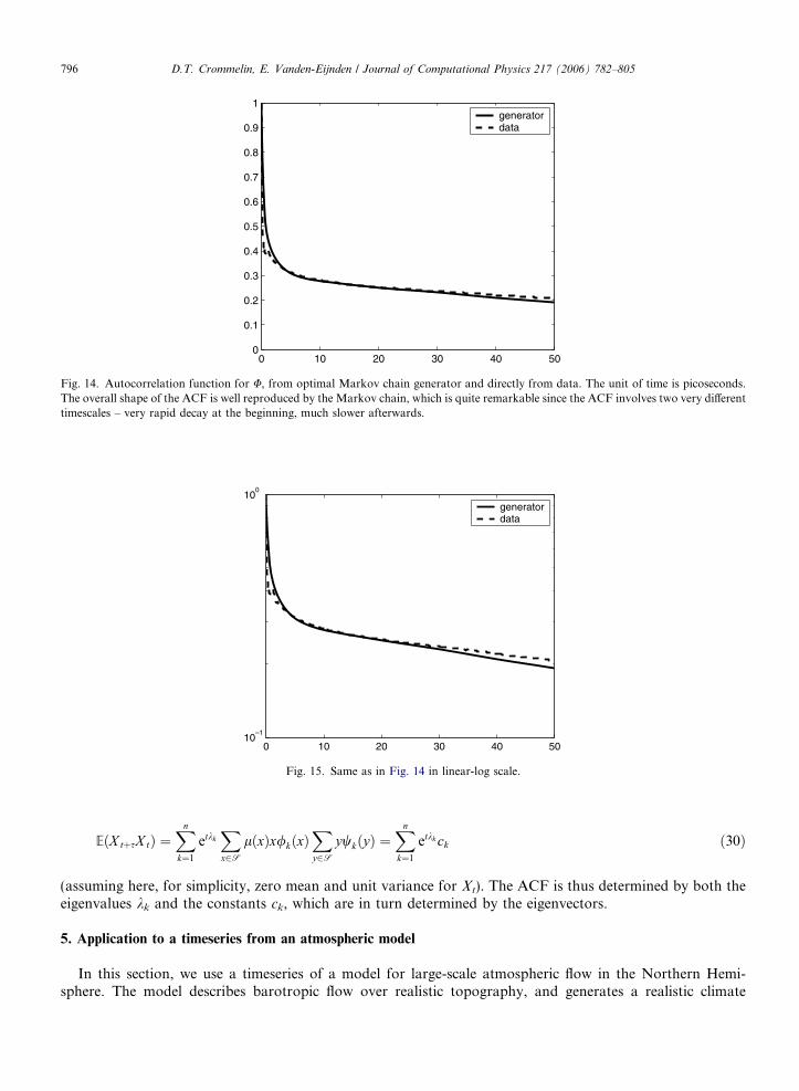
E!X t$sX t" #Xn

k#1

etkkX

x2Sl!x"x/k!x"

X

y2Sywk!y" #

Xn

k#1

etkk ck !30"

(assuming here, for simplicity, zero mean and unit variance for Xt). The ACF is thus determined by both theeigenvalues kk and the constants ck, which are in turn determined by the eigenvectors.

5. Application to a timeseries from an atmospheric model

In this section, we use a timeseries of a model for large-scale atmospheric flow in the Northern Hemi-sphere. The model describes barotropic flow over realistic topography, and generates a realistic climate

0 10 20 30 40 500

0.1

0.2

0.3

0.4

0.5

0.6

0.7

0.8

0.9

1generatordata

Fig. 14. Autocorrelation function for U, from optimal Markov chain generator and directly from data. The unit of time is picoseconds.The overall shape of the ACF is well reproduced by the Markov chain, which is quite remarkable since the ACF involves two very di!erenttimescales – very rapid decay at the beginning, much slower afterwards.

0 10 20 30 40 5010

–1

100

generatordata

Fig. 15. Same as in Fig. 14 in linear-log scale.


using 231 variables (wavenumber truncation T21). A more detailed description of the model, its physicalinterpretation and its dynamics is given in [17]. As is usually the case in models for large-scale flow, muchof the interesting dynamics is captured by a fairly low number of leading modes of variability (PrincipalComponents, or PCs). Describing the dynamics of the leading PCs without explicitly invoking the other,trailing PCs is a challenging and well-known problem; one that we aim to tackle here using a continuous-time Markov chain description (see also [18–20] for di!erent approaches to arrive at a reduced descriptionof the dynamics of the leading modes of variability of the same atmospheric model). Since we resolve onlyone or two variables out of a total of 231, without a clear timescale separation between resolved and unre-solved variables, non-Markov e!ects are important in this situation. It is far from obvious that a Markovchain can be successful at all under these circumstances.

Although the use of continuous-time Markov chains is rare in atmosphere-ocean science, the use of dis-crete-time Markov chains is not. Examples can be found in [21–25] and many more studies.

0 50 100 150 200–0.1

–0.09

–0.08

–0.07

–0.06

–0.05

–0.04

–0.03

–0.02

–0.01

0

lag h in days

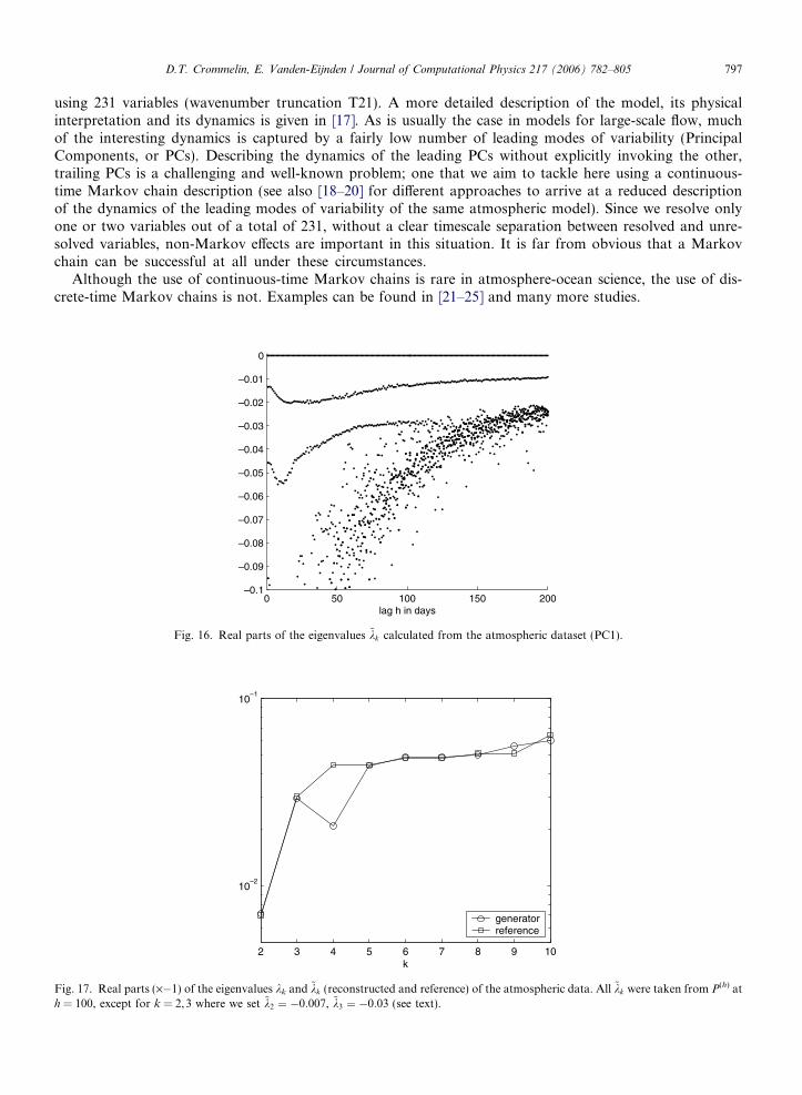
Fig. 16. Real parts of the eigenvalues ~kk calculated from the atmospheric dataset (PC1).

2 3 4 5 6 7 8 9 10

10–2

10–1

k

generatorreference

Fig. 17. Real parts (·%1) of the eigenvalues kk and ~kk (reconstructed and reference) of the atmospheric data. All ~kk were taken from P(h) ath = 100, except for k = 2,3 where we set ~k2 # %0:007, ~k3 # %0:03 (see text).


5.1. One-dimensional situation

For the one-dimensional case the leading principal component (PC1) is used; in Section 5.2 we consider thetwo-dimensional case, using PC1 and PC3. A total of 107 datapoints is available, with a timestep h = 1 whichis interpreted as 1 day.

The state space for PC1 is discretized into 10 bins, which we interpret as the 10 states of the state-space S.The timeseries is binned accordingly, and we calculate ~P !h" from (8) and its eigenspectrum for all lags1 6 h 6 200. The real parts of the (leading) eigenvalues ~kk are shown in Fig. 16. Eigenvalues withRe~kk < %0:1 are not shown, since we are primarily interested in the leading eigenvalues. As can be seen, ~k2and ~k3 (both are real) drop in value over the range 1 6 h 6 10, then go up again. Only for long lags(h ( 200 for ~k2, h ( 100 for ~k3) do they reach values that are consistent with the ACF for PC1 (shown inFig. 20): ~k2 # %0:007, ~k3 # %0:03. For even longer lags, the estimates for ~k2 and ~k3 eventually become over-whelmed by sampling error. For ~k3 this can be seen to happen for h > 100 (Fig. 16), for ~k2 it lies beyond thelimits of the figure.

With Fig. 16 in mind, we set ~k2 # %0:007, ~k3 # %0:03 by hand, and use the spectrum of ~P !h" at h = 100 forthe other eigenvalues and for all eigenvectors. Other than for the molecular data in the previous section, thelag h = 1 is too low in this case, because h = 1 is below the slowest of the fast timescales of the system. If datafrom h = 1 is used, these fast timescales negatively a!ect the e!ective description of the slow dynamics. Ath = 100 this is no longer a problem.

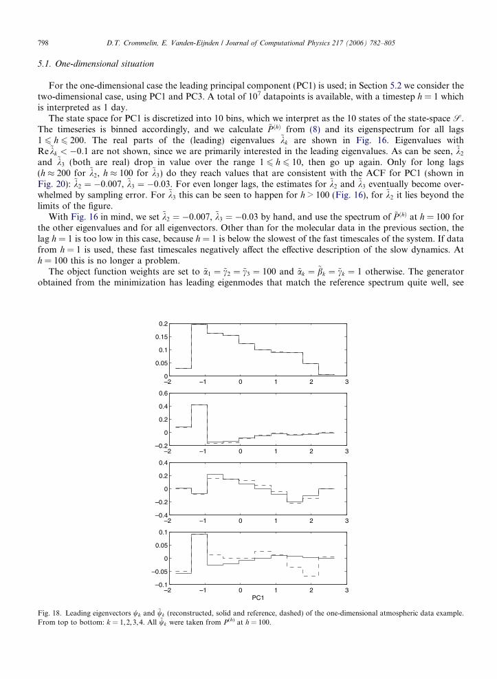
The object function weights are set to ~a1 # ~c2 # ~c3 # 100 and ~ak # ~bk # ~ck # 1 otherwise. The generatorobtained from the minimization has leading eigenmodes that match the reference spectrum quite well, see

–2 –1 0 1 2 30

0.05

0.1

0.15

0.2

–2 –1 0 1 2 3–0.2

0

0.2

0.4

0.6

–2 –1 0 1 2 3–0.4

–0.2

0

0.2

0.4

–2 –1 0 1 2 3–0.1

–0.05

0

0.05

0.1

PC1

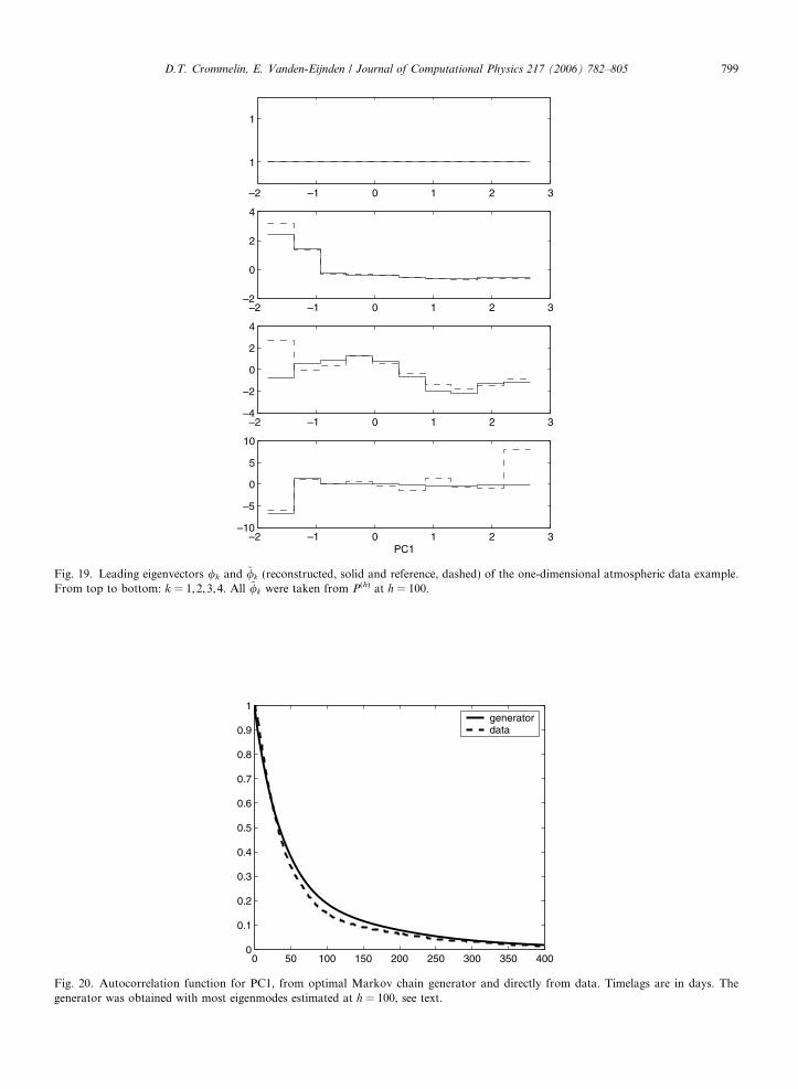
Fig. 18. Leading eigenvectors wk and ~wk (reconstructed, solid and reference, dashed) of the one-dimensional atmospheric data example.From top to bottom: k = 1,2,3,4. All ~wk were taken from P(h) at h = 100.


–2 –1 0 1 2 3

1

1

–2 –1 0 1 2 3–2

0

2

4

–2 –1 0 1 2 3–4

–2

0

2

4

–2 –1 0 1 2 3–10

–5

0

5

10

PC1

Fig. 19. Leading eigenvectors /k and ~/k (reconstructed, solid and reference, dashed) of the one-dimensional atmospheric data example.From top to bottom: k = 1,2,3,4. All ~/k were taken from P(h) at h = 100.

0 50 100 150 200 250 300 350 4000

0.1

0.2

0.3

0.4

0.5

0.6

0.7

0.8

0.9

1generatordata

Fig. 20. Autocorrelation function for PC1, from optimal Markov chain generator and directly from data. Timelags are in days. Thegenerator was obtained with most eigenmodes estimated at h = 100, see text.


0 50 100 150 200 250 300 350 40010

–2

10–1

100

generatordata

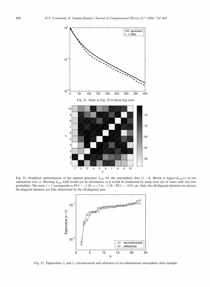
Fig. 21. Same as Fig. 20 in linear-log scale.

1 2 3 4 5 6 7 8 9 10

1

2

3

4

5

6

7

8

9

10

x

y

–30

–25

–20

–15

–10

Fig. 22. Graphical representation of the optimal generator Lmin for the atmospheric data (1 % d). Shown is log[l(x)Lmin(x,y)] (nosummation over x). Showing Lmin itself would not be informative as it would be dominated by jump rates out of states with very lowprobability. The state x = 1 corresponds to PC1 < %1.38, x = 2 to %1.38 < PC1 < %0.93, etc. Only the o!-diagonal elements are shown;the diagonal elements are fully determined by the o!-diagonal ones.

0 5 10 15 20 25

10–2

10–1

k

Eig

enva

lue

(x –

1)


Fig. 23. Eigenvalues kk and ~kk (reconstructed and reference) of two-dimensional atmospheric data example.


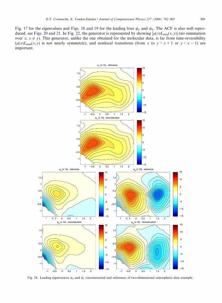
Fig. 17 for the eigenvalues and Figs. 18 and 19 for the leading four wk and /k. The ACF is also well repro-duced, see Figs. 20 and 21. In Fig. 22, the generator is represented by showing [l(x)Lmin(x,y)] (no summationover x; x 6# y). This generator, unlike the one obtained for the molecular data, is far from time-reversibility(l(x)Lmin(x,y) is not nearly symmetric), and nonlocal transitions (from x to y > x + 1 or y < x % 1) areimportant.

Fig. 24. Leading eigenvectors wk and ~wk (reconstructed and reference) of two-dimensional atmospheric data example.


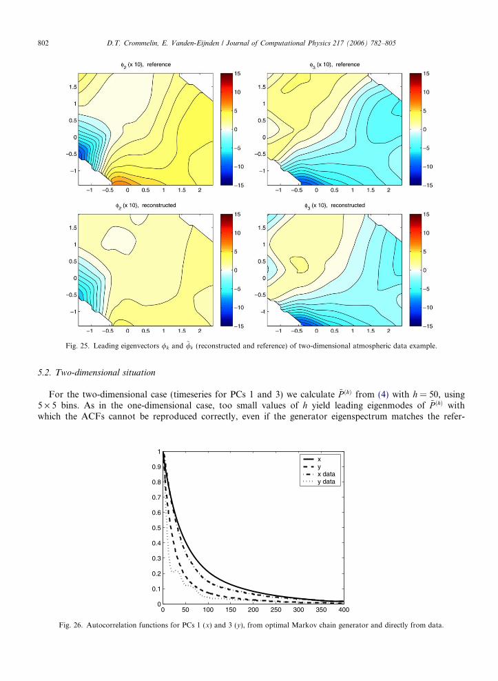
5.2. Two-dimensional situation

For the two-dimensional case (timeseries for PCs 1 and 3) we calculate ~P !h" from (4) with h = 50, using5 · 5 bins. As in the one-dimensional case, too small values of h yield leading eigenmodes of ~P !h" withwhich the ACFs cannot be reproduced correctly, even if the generator eigenspectrum matches the refer-

Fig. 25. Leading eigenvectors /k and ~/k (reconstructed and reference) of two-dimensional atmospheric data example.

0 50 100 150 200 250 300 350 4000

0.1

0.2

0.3

0.4

0.5

0.6

0.7

0.8

0.9

1xyx datay data

Fig. 26. Autocorrelation functions for PCs 1 (x) and 3 (y), from optimal Markov chain generator and directly from data.


ence spectrum perfectly. Because of the higher number of bins than used in the one-dimensional case,sampling errors for ~P !h" are too large at h = 100. Therefore we use a smaller lag, h = 50. The leadingeigenvalue ~k2 is again adjusted to %0.007 (just as in the one-dimensional case); ~k3 # %0:033 at h = 50and is not further adjusted. Two of the bins remain empty, so e!ectively the state space is discretized into23 bins. The object function weights are the same as in the one-dimensional case (~ak # ~bk # ~ck # 1 "k,except ~a1 # ~c2 # ~c3 # 100).

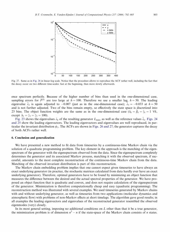
Fig. 23 shows the eigenvalues kk of the resulting generator Lmin, as well as the reference values ~kk. Figs. 24and 25 show the leading eigenvectors. The leading eigenvectors and eigenvalues are well reproduced, in par-ticular the invariant distribution w1. The ACFs are shown in Figs. 26 and 27; the generator captures the decayof both ACFs rather well.

6. Conclusion and generalization

We have presented a new method to fit data from timeseries by a continuous-time Markov chain via thesolution of a quadratic programming problem. The key element in the approach is the matching of the eigen-spectrum of the generator with the eigenspectrum observed from the data. Since the eigenspectrum completelydetermines the generator and its associated Markov process, matching it with the observed spectrum, if suc-cessful, amounts to the most complete reconstruction of the continuous-time Markov chain from the data.Matching of the observed invariant distribution is part of this reconstruction.

The Markov chain embedding problem implies that one cannot expect given timeseries to have always anexact underlying generator (in practice, the stochastic matrices calculated from data hardly ever have an exactunderlying generator). Therefore, optimal generators have to be found by minimizing an object function thatmeasures the di!erence between the desired and the actual spectral properties of the generator. We have pro-posed an object function that is quadratic and convex, and does not require calculation of the eigenspectrumof the generator. Minimization is therefore computationally cheap and easy (quadratic programming). Thereconstruction method was illustrated with several examples. We used timeseries generated by Markov chainswith and without underlying generator, as well as timeseries from two applications (molecular dynamics andatmospheric flow) with problems of non-Markov e!ects at short timelags. The algorithm gave good results; inall examples the leading eigenvectors and eigenvalues of the reconstructed generator resembled the observedeigenmodes (very) closely.

In its most general setting, imposing no additional conditions on L other than that it be a true generator,the minimization problem is of dimension n2 % n if the state-space of the Markov chain consists of n states.

0 50 100 150 200 250 300 350 40010

–3

10–2

10–1

100

xyx datay data

Fig. 27. Same as in Fig. 26 in linear-log scale. Notice that the procedure allows to reproduce the ACF rather well, including the fact thatthe decay occur on two di!erent time-scales: fast at the beginning, then more slowly afterwards.


However, by restricting the class of Markov chain generators, the dimensionality of the problem can bereduced without reducing the size of the state-space. For example, the assumption of detailed balance,l(x)L(x,y) = l(y)L(y,x), eliminates half of the variables from the minimization problem: only the matrix ele-ments L(x,y) with x > y need to be determined. Detailed balance is a non-trivial assumption; for instance, theoptimal generator found for the molecular data is close to detailed balance, whereas the generators for theatmospheric data are not. Another example of restricting the class of generators would be to impose the struc-ture of a birth-death process. Such a process is characterised by a generator of the type:

X

y2SL!x; y"f !y" #

Xm

j#1

mj!x"!f !x$ ej" % f !x""; !31"

where mj(x)P 0 are constants, and ej are such that x$ ej 2 S if mj(x) 6# 0 and, typically, m is (much) smallerthan n. One would then fix the ej and minimize the object function (13) over all possible mj(x) subject tomj(x) P 0. The dimensionality of this minimization problem is mn, which is substantially smaller thann2 % n if m ) n. In terms of implementation, it is a completely straightforward generalization of what wasdone in this paper.

Notice in particular that a structure like (31) for the generator is quite natural for systems in which jumpscan only occur between states x and y which correspond to neighboring bins in physical space. These consid-erations lead us to the possibility of generalizing the reconstruction procedure, outlined in this paper for finitestate Markov chains, to di!usion processes. An appropriate discretization of the Fokker–Planck operatorusing e.g. finite-di!erences or finite-elements will convert the problem of reconstructing the drift and di!usioncoe"cients into the problem of reconstructing a generator with a structure similar to the one in (31). The pro-cedure proposed here can be used to tackle the latter problem, and thereby reconstruct the drift and di!usionin spatially discretized form. We intend to explore this approach to the reconstruction of di!usion processes ina future study.

Acknowledgments

We thank Christian Franzke for providing us with the timeseries of the atmospheric model, and PaulMaragakis for making his molecular simulation data available. Helpful comments and suggestions from AndyMajda are gratefully acknowledged. We also thank Weinan E, Paul Maragakis, Weiqing Ren, and RichardTsai for helpful discussions when this project was at an early stage. This work was sponsored in part byNSF through Grants DMS01-01439, DMS02-09959, DMS02-39625 and DMS-0222133, and by ONR throughGrants N-00014-04-1-0565 and N-00014-96-1-0043.

References

[1] J. Norris, Markov Chains, Cambridge University Press, Cambridge, 1997.[2] O. Haggstrom, Finite Markov Chains and Algorithmic Applications, Cambridge University Press, Cambridge, 2002.[3] W. Anderson, Continuous-Time Markov chains, Springer, Berlin, 1991.[4] J. Kingman, The imbedding problem for finite Markov chains, Z. Wahrsch. 1 (1962) 14–24.[5] B. Singer, S. Spilerman, The representation of social processes by Markov models, Am. J. Sociol. 82 (1976) 1–54.[6] R. Israel, J. Rosenthal, J. Wei, Finding generators for Markov chains via empirical transition matrices, with applications to credit

ratings, Math. Finance 11 (2001) 245–265.[7] M. Bladt, M. Sørensen, Statistical inference for discretely observed Markov jump processes, J. R. Statist. Soc. B 67 (2005) 395–410.[8] P. Gill, W. Murray, M. Wright, Practical Optimization, Academic Press, New York, 1981.[9] J. Nocedal, S. Wright, Numerical Optimization, Springer, Berlin, 1999.[10] T. Anderson, L. Goodman, Statistical inference about Markov chains, Ann. Math. Statist. 28 (1957) 89–110.[11] B.R. Brooks, R.E. Bruccoleri, B.D. Olafson, D.J. States, S.S. Swaminathan, M. Karplus, CHARMM: a program for macromolecular

energy, minimization, and dynamics calculations, J. Comput. Chem. 4 (1983) 187–217.[12] W. Huisinga, C. Schutte, A. Stuart, Extracting macroscopic stochastic dynamics: model problems, Commun. Pure Appl. Math. 56

(2003) 234–269.[13] G. Hummer, I.G. Kevrekidis, Coarse molecular dynamics of a peptide fragment: free energy, kinetics, and long-time dynamics

computations, J. Chem. Phys. 118 (2003) 10762.[14] P.G. Bolhuis, C. Dellago, D. Chandler, Reaction coordinates of biomolecular isomerization, Proc. Natl. Acad. Sci. USA 97 (2000)

5877–5882.


[15] J. Apostolakis, P. Ferrara, A. Caflisch, Calculation of conformational transitions and barriers in solvated systems: application to thealanine dipeptide in water, J. Chem. Phys. 10 (1999) 2099–2108.

[16] W. Ren, E. Vanden-Eijnden, P. Maragakis, W. E, Transition pathways in complex systems: application of the finite-temperaturestring method to the alanine dipeptide, J. Chem. Phys. 123 (2005) 134109.

[17] D. Crommelin, Regime transitions and heteroclinic connections in a barotropic atmosphere, J. Atmos. Sci. 60 (2003) 229–246.[18] F. Selten, An e"cient description of the dynamics of barotropic flow, J. Atmos. Sci. 52 (1995) 915–936.[19] F. Kwasniok, The reduction of complex dynamical systems using principal interaction patterns, Physica D 92 (1996) 28–60.[20] C. Franzke, A. Majda, E. Vanden-Eijnden, Low-order stochastic mode reduction for a realistic barotropic model climate, J. Atmos.

Sci. 62 (2005) 1722–1745.[21] K.C. Mo, M. Ghil, Cluster analysis of multiple planetary flow regimes, J. Geophys. Res. 93 (1988) 10927–10952.[22] R. Vautard, K.C. Mo, M. Ghil, Statistical significance test for transition matrices of atmospheric Markov chains, J. Atmos. Sci. 47

(1990) 1926–1931.[23] R. Pasmanter, A. Timmermann, Cyclic Markov chains with an application to an intermediate ENSO model, Nonlin. Proc. Geophys.

10 (2003) 197–210.[24] G. Lacorata, R. Pasmanter, A. Vulpiani, Markov chain approach to a process with long-time memory, J. Phys. Oceanogr. 33 (2003)

293–298.[25] D. Crommelin, Observed nondi!usive dynamics in large-scale atmospheric flow, J. Atmos. Sci. 61 (2004) 2384–2396.


fitting timeseries by continuous-time markov …eve2/tseries_jcp.pdffitting timeseries by...

Documents