finite volume solutions of convection-diffusion test problems€¦ · finite volume solutions of...

mathematics of computationvolume 60, number 201january 1992, pages 189-220

FINITE VOLUME SOLUTIONS

OF CONVECTION-DIFFUSION TEST PROBLEMS

J. A. MACKENZIE AND K. W. MORTON

Abstract. The cell-vertex formulation of the finite volume method has been

developed and widely used to model inviscid flows in aerodynamics: more re-

cently, one of us has proposed an extension for viscous flows. The purpose of

the present paper is two-fold: first we have applied this scheme to a well-known

convection-diftusion model problem, involving flow round a 180° bend, which

highlights some of the issues concerning the application of the boundary con-

ditions in such cell-based schemes. The results are remarkably good when the

boundary conditions are applied in an appropriate manner. In our efforts to

explain the high quality of the results we were led to a detailed analysis of the

corresponding one-dimensional problem. Our second purpose is thus to gather

together various approaches to the analysis of this problem and to draw atten-

tion to the supra-convergence phenomena enjoyed by the proposed methods.

1. Introduction

Since their independent introduction by McDonald [14] and MacCormack

and Paullay [11] for the discretization of the transonic Euler equations, finite

volume methods have taken a leading role in computational fluid dynamics. The

more recent popularization of these methods by Jameson et al. [7], Ni [21] andothers has now established them as the dominant discretization schemes in the

computation of aeronautical fluid flows. Over the years there have been many

variants of the finite volume method, but two main types of formulation have

emerged. In the cell-center approach, associated with the name of Jameson,although he has used both successfully, values of the unknowns are held at

the centers of the cells over which conservation is imposed. In the cell-vertex

scheme they are held at the vertices of these same cells. This presupposes that

we are using quadrilateral cells in two dimensions, or hexahedral cells in three

dimensions.

Morton and Paisley [ 18] have given good reasons, stemming mainly from the

greater compactness of the stencil, why the cell-vertex formulation should be

preferred for modeling inviscid flows. On the other hand, for viscous flows,

modelled by the Navier-Stokes equations, one might expect the advantage to

lie with the cell-center methods. However, we shall show that our cell-vertex

Received by the editor June 13, 1991.1991 Mathematics Subject Classification. Primary 65N99, 65L10; Secondary 76M25, 76R05.Key words and phrases. Convection-diffusion, finite volume, cell-vertex.

The work reported here forms a part of the research programme of the Oxford-Reading Institute

for Computational Fluid Dynamics.

©1992 American Mathematical Society

0025-5718/92 $1.00 + $.25 per page

189

License or copyright restrictions may apply to redistribution; see http://www.ams.org/journal-terms-of-use

190 J. A. MACKENZIE AND K. W. MORTON

scheme has some attractive properties in this case too. This paper has arisen

from an investigation of the performance of the scheme for two well-known

convection-diffusion test problems, proposed at an IAHR workshop, the results

of which are summarized by Smith and Hutton [23].

2. The cell-vertex method

We begin by describing the cell-vertex method for the steady convection-

diffusion problem

(2.1a) V • (eVw - a«) = / inQ,

(2.1b) u = g onrD,

and

(2.1c) du/dn = 0 onTN,

where e is a positive diffusion coefficient and a = (a, b)T is the convective

velocity field. The domain Si is an open bounded region of IR with boundary

TD u TN. We assume that the domain is partitioned by a structured mesh

of quadrilaterals and suppose, for simplicity, that its vertices can be labelled

{ii,j)\i = 0,l,...,M;j = 0,l,...,N}.Noting that the left-hand side of problem (2.1a) can be considered as the

divergence of a vector flux function W = (F, G) with F = eux - au and

G = euy - bu, we can obtain an algebraic equation for each interior cell by

integrating (2.1a) over the cell, using the divergence theorem to convert this

into line integrals of normal fluxes along the cell edges, and approximating

these using the trapezoidal rule: for cell C of Figure 1(a),

/ div(F, G) dxdy = [ Fdy -GdxJc JdC

(2-2) _ 12[(Ei - P})(y2 - V4) + (¿="2 - F4)(yi - vi)

- (G. - G3)(x2 - x4) - (G2 - G4)(x3 - xx )].

With the approximation U(x,y) parametrized by its values U¡j at the

vertices, this still leaves Vu to be approximated at the same points. There

are several ways in which this may be done, but we consider mainly that called

Method A in Mackenzie [12]. That is, each component of Vu is also considered

as a divergence, and its value at the vertex is obtained as an average over the

subsidiary quadrilateral centered at that point and obtained by integrating along

the diagonals as in Figure 1(b). Thus we have

<"' %

<"' I

1

2VxU\x) := ^[(Ue - Uw)(yN-ys) + (UN - Us)(yw - yE)),

V\y) := -^y[(UE - Uw)(xN-xs) + (UN - Us)(xw - xE)\.


FINITE VOLUME SOLUTIONS OF CONVECTION-DIFFUSION TEST PROBLEMS 191

(a) (b)

Figure 1. Geometric configuration of flow variables: (a) the

conservation cell C; (b) the subblock used for a derivative at 1

On a rectangular uniform grid, approximations (2.3) and (2.4) coincide with the

standard second-order central difference formulae. To complete the approxima-

tion over cell C, the right-hand side of (2. la) is assumed to be integrated exactly.

It remains to consider how boundary conditions are to be imposed and the

set of cell residual equations assembled so as to yield a nonsingular system.

We suppose that for the differential system u is prescribed at some points,

including all those corresponding to inflow, and otherwise the homogeneous

Neumann condition du/dn = 0 is to be imposed. For the discrete system

we shall assume that P boundary vertices have their values prescribed and

that P > M + N + I, that is, that at least half are prescribed. Then thetotal number of unknowns is (M + l)(N + 1) - P < MN, so that there are

sufficient cell equations that may be used to determine them: to obtain an exact

match, various algorithms may be used. We prefer one based on upwinded

control volumes used in the Moores' method [15], but derived through a Petrov-

Galerkin formulation. The derivation starts from the Galerkin equations, which

associate each nodal unknown with its test function, which is identical to a

piecewise linear trial function. Then, this is replaced by a piecewise constant

test function over a quadrilateral—as in a cell-centered finite volume method.

Finally, this is shifted upwind to coincide with one of the four cells meeting

at the node. The upwinding is based on the convective velocity at the node

and results in each nodal unknown being associated with just one cell residual.

We shall confine our consideration here to cases where, in turn, each interior

cell residual is associated in this way with just one unknown: there may be

some boundary cells, where Dirichlet conditions are imposed and the flow is

directed outwards, which are not associated with unknowns and their residuals

will not be used. A form of the allocation algorithm which will deal with all

flow situations is given in Morton [17].

For the boundary edges, the normal flux is approximated as follows: first

the derivative along each edge can be approximated by the divided difference

in that direction, (Up - Uq)/\tp - re| in Figure 2; then the derivative alongthe adjoining edge at each boundary vertex is extrapolated from the divided



R R

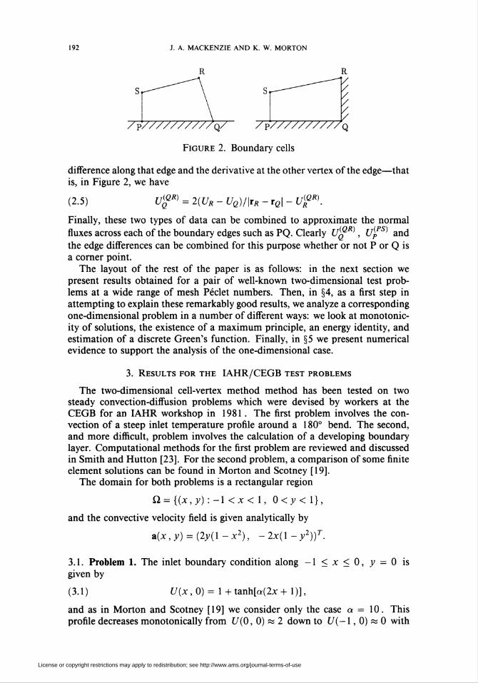
Figure 2. Boundary cells

difference along that edge and the derivative at the other vertex of the edge—that

is, in Figure 2, we have

(2.5) ufR) = 2(UR - UQ)/\rR - re| - ufR).

Finally, these two types of data can be combined to approximate the normal

fluxes across each of the boundary edges such as PQ. Clearly Uq*R), UPPS) and

the edge differences can be combined for this purpose whether or not P or Q is

a corner point.

The layout of the rest of the paper is as follows: in the next section we

present results obtained for a pair of well-known two-dimensional test prob-

lems at a wide range of mesh Péclet numbers. Then, in §4, as a first step in

attempting to explain these remarkably good results, we analyze a corresponding

one-dimensional problem in a number of different ways: we look at monotonic-

ity of solutions, the existence of a maximum principle, an energy identity, and

estimation of a discrete Green's function. Finally, in §5 we present numerical

evidence to support the analysis of the one-dimensional case.

3. Results for the IAHR/CEGB test problems

The two-dimensional cell-vertex method method has been tested on two

steady convection-diffusion problems which were devised by workers at the

CEGB for an IAHR workshop in 1981. The first problem involves the con-vection of a steep inlet temperature profile around a 180° bend. The second,

and more difficult, problem involves the calculation of a developing boundary

layer. Computational methods for the first problem are reviewed and discussed

in Smith and Hutton [23]. For the second problem, a comparison of some finite

element solutions can be found in Morton and Scotney [19].

The domain for both problems is a rectangular region

Si = {ix,y):-l <x <l, 0<y<l},

and the convective velocity field is given analytically by

a(x,y) = (2y(l-x2), -2x(l-y2))T.

3.1. Problem 1. The inlet boundary condition along -1 < x < 0, y = 0 is

given by

(3.1) i/(x,0) = l + tanh[a(2x+l)],

and as in Morton and Scotney [19] we consider only the case a = 10. This

profile decreases monotonically from U(0, 0) « 2 down to U(—\, 0) « 0 with


finite volume solutions of convection-diffusion test PROBLEMS 193

Figure 3. Streamlines for the IAHR/CEGB problems: hashingindicates unused cell residuals at outflow Dirichlet boundaries

a very steep interior layer centered at (-1/2,0). The boundary condition on

the tangential boundaries, x = -I, y = I and x = 1 is given by the compatible

Dirichlet condition U = I - tanh(a). Finally, a homogeneous Neumann or

natural boundary condition is imposed at the outlet 0 < x < 1, y = 0. For

comparison with Smith and Hutton [23], the calculations are performed on auniform grid Ax = Ay = 0.1 . The main test of this problem is the calculationof the outflow profile for a wide range of values of e . Here, we have considered

e = 1 x 10-6, 2 x 10~3, 1 x 10~2, and 1 x 10"1 and with max|a| = 2 thisgives a range of cell Péclet numbers from 2 to 2 x 105. To effectively cover

all cases on such a coarse grid is a very severe test for any method: the high

curvature of the velocity field near the origin can easily introduce errors due to

crosswind diffusion.

For the problem on a M x N grid there are potentially (M + 1) x (N + 1)

unknowns. Here we have P = 2(AT + 1) + Af — 1 + M/2 Dirichlet bound-ary conditions, and since P > M + N + 1, we therefore have sufficient cellequations to determine the unknowns. To obtain an exact match between the

unknowns and cell equations, we follow the procedure given in §2. Labelling

the (i, 7')th cell equation from the bottom left, this results in each equation

being associated with just one unknown except for the M/2 cell equations

(l = 1, ... , M/2 ; j = N) and the N cell equations (/' = M ; j = I, ... , N)which are disregarded—see Figure 3; to resolve the ambiguity in the association

of the nine nodal unknowns on x = 0 one has to appeal to the curvature of the

streamlines. To approximate the normal fluxes along the boundary edges, a sim-

plification of the extrapolation procedure described in §2 can be used because

of the uniform rectangular mesh.

For comparison, an accurate solution was calculated using a finite difference

method on a fine grid where Ax = Ay = 0.02 and the computed output profiles,restricted onto the coarse grid, are shown in Figure 4(a). The results using

the cell-vertex method on the standard grid are given in Figure 4(b) and are

remarkably good. For the two largest cell Péclet number cases the solutions are

sharp and have little or no undershoots or overshoots and are as accurate as

one could expect on such a coarse grid. The capability of the cell-vertex finite



MESH SIZE = 0.02

DIFFUSION-0.1E-05

-0.2E-02

-0.1E-01

0.1E+00

(a)

MESH SIZE - 0.1

DIFFUSION-0.1E-05

-0.2E-02

-0.1E-01

-0.1E+00

(b)

Figure 4. Outlet profiles for first IAHR/CEGB test problem:(a) shows the finite difference fine grid solution restricted to the

coarse grid; (b) is the cell-vertex finite volume solution on the

standard grid

volume method to cope with viscous dominated problems is demonstrated by

the solutions of the remaining two cases, which are at least as accurate as the

solutions obtained from other methods. Note that no upwinding parameters,

depending on the cell Péclet number, are used in this method—in contrast to

the many well-known exponential-fitting methods, Petrov-Galerkin schemes, or

upwind difference schemes.



lv-0-9l 100

so

60

40

0.4 0.8

6 = 1 X 10"1 £ = 1 X 10"2 e = 2 x 10~3 e= 1 x 10"

w

0.84 0.88 0.92 0.96 0.84 0.88 0.92 0.96

(b)

Figure 5. (a) shows the finite volume boundary layer solutions

for different values of e for the second IAHR/CEGB problem;

(b) compares the fine and coarse grid solutions at y = 0.0 and

y = 0.5 with e = 2 x 10-3



3.2. Problem 2. The second test case considered is a modification of the first

problem where the inlet profile is now given by í/(jc , 0) = 0 and on the right-

hand tangential boundary, x = 1, the Dirichlet condition ¿7(1, y) = 100,0 < y < 1, is imposed. The compatible Dirichlet condition U = 0 is alsoset on the remaining two boundaries x = -1 and y = 1 . The main difficulty

of this problem lies in the calculation of a developing boundary layer from

the corner point x = I, y = I to the outflow y = 0. Figure 5(a) (see p.

195) shows the computed solutions using the finite volume method at the three

stations y = 0.9, y = 0.5 and y = 0, for the four values of e which were

considered in the first problem.

The results for the two lower values of the cell Péclet number agree well with

streamline-diffusion [6], upwinded [5] and the mixed finite element solutions

found in Morton and Scotney [19]. In fact, the finite volume solutions bear a

remarkable resemblance to those obtained by the mixed finite element method

proposed by Morton and Scotney. For the higher cell Péclet number cases the

story is quite different. For instance, when e = 2 x 10~3 the thickness of

the boundary layer only extends to two cell widths of the standard mesh. On

such a coarse grid the finite volume method has performed extremely well and

has successfully modelled the thickening of the boundary layer. More detailed

pictures of the solution at y = 0.0 and y = 0.5 are given in Figure 5(b)

where the standard grid solutions are compared with a solution on a 40 x 20

nonuniform grid which has been stretched into the boundary layer. In Morton

and Scotney [ 19] it was found that the streamline-diffusion and upwinded finite

element methods, which both aim at giving positive monotone solutions to this

problem, completely failed to model the boundary layer for this value of e.

When e = 1 x 10-6 the boundary layer is so thin that it cannot be represented

on the standard mesh. However, the finite volume method still gives a positive

monotone solution which is in stark contrast to the oscillatory behavior of theaforementioned finite element solutions.

The combination of accuracy and monotonicity of the cell-vertex method

for both problems makes this method extremely attractive and practicable. In

the following sections we attempt to examine the method in more detail by

analyzing the one-dimensional version of the scheme.

4. Analysis for a one-dimensional problem

In this section we consider the solution of the following two-point boundary

value problem:

Luix) = ¿du

8^-audx

= f, X£Si = i0,l),

(4.1)

w(0) = 0, w(l) = l,

where e and a are positive constants with 0 < e < 1. Although this singular

perturbation problem can be solved exactly, we consider it as the simplest model

problem for more complicated singular perturbation problems leading to the

Navier-Stokes equations at high Reynolds numbers. We shall also consider

generalizations of this problem in which a is replaced by a positive function

a(x). It turns out that this seemingly innocuous problem is extremely difficult



to analyze to sufficient precision to demonstrate all the attractive properties of

the cell-vertex scheme.

4.1. The finite volume schemes in ID. We define a grid, Ylh , as a partition of

the unit interval [0, 1 ], where

flft = {0 = x0 < xx < ••■ < xN-X < Xn = 1},

which has a variable step size hj = Xj - Xj-X and where we set h = max7 h¡.

On this grid we define the usual difference operators

(4.2) A±Uj = ±iU}±x-Uj), D+Uj = ^ and D.U] = ¿^.nj+x hj

The cell-vertex approximation is obtained by integrating (4.1) over the first

N - 1 control volumes to get

(4.3) e(U'j - U'j_x) - a(Uj - £/,_,) = P fdx, j=l,...,N-l,Jxj-i

where C/j represents an approximation to u'(Xj). If we divide through both

sides by hj we arrive at the discrete equivalent of (4.1); that is Lh : Xn —> Y„

is defined by

(4.4) (LhU)j = UeiU; - U]_x) - ajiUj - (7,_,)] = ¡- P fdx = ifh)j.nj nj Jxj-i

Here, Xn and Yn are simply IR^-1 equipped with suitable norms. Two ap-

proximations of the gradient are summarized as follows:

(4.5) U'j = [ajD+ + ( 1 - aj)D-]Uj , 1 < j < N - 1,

where a¡ = hj+x/(hj + hJ+x) corresponds to Method A of Mackenzie [12] and

ctj = hj/(hj + hj+x) corresponds to Method B: note that in Method A we have

U'j = (Uj+x - Uj-X)/ihj + hj+x). The derivative at x = 0 is given by a second-

order extrapolation of the gradient from the interior of the domain, that is,

(4.6) U¿ = 2D.UX -U[.

Note that both of the above schemes involve a four- and a two-point approxi-

mation to the second- and first-derivative terms, respectively, and are identical

when the grid is uniform. Gushchin and Shchennikov [4] and Lavery [ 10] have

considered this scheme on a uniform mesh, both of them in connection with

nonoscillatory solutions of two-point boundary value problems.

4.2. Approximation of boundary layers and control of spurious solution modes.

The most commonly used first- and second-order schemes reduce to a three-

point difference scheme for the ID model problem (4.1 ). The cell-vertex scheme,

however, uses four points centered on an interval. This results in the scheme

having a spurious solution mode for the homogeneous equation, which has to

be controlled by the extra boundary condition (4.6) used at the inflow end. So

we start our consideration of this scheme with the homogeneous problem on auniform mesh.



When f = 0 the analytical solution of (4.1) is

eax/e _ j

(4.7) u(x) =ea/e _ 1

which increases monotonically and has a steep boundary layer of thickness 0(e)

at x = 1.On a uniform mesh, Methods A and B are identical with a, = 1/2 for all j .

The exact solution of the difference equations (4.3) with the boundary condition

(4.6) can then be written as

lt[-l + *(jd-l)

where

ßx = ß + (i + ß2y/2, p2 = ß-(i + ß2)1'2,

V 1 - Pi ) P2

and ß = ah/e is the cell Péclet number. Note that px > 1 and is a second-

order approximation to e? . However, -1 < p2 < 0, and p2 is the expected

oscillatory solution mode; but this mode decays for increasing j, and an im-

portant feature of the scheme is that the resulting solution is monotonie. This

is proved in Theorem 4.1.

For the standard three-point central difference scheme,

(UJ+x-2Uj + Uj_x) jUj+i-Uj_i)(LhU)j-e-¡-j-a-Yh-,

the solution of the difference equations is

p{-I 1 + 4(4.9) U*-■$=»' wher^3 = TTl

is the (1,1 )-Padé approximant of e^ which is also second-order accurate.

However, unless ß < 2, we have p¿ < 0, and the solution is oscillatory and

growing. This condition is very restrictive when e is small and therefore, al-

though the scheme has no spurious modes, the approximation is poor as e —► 0

for a fixed h .For the standard first-order upwind finite difference scheme,

iUJ+i-2Uj + Uj_i) (Uj-Uj-i)\^hu )j — fc ^2 h '

we have

(4.10) Uj = ßAN~ , where pA = l+ ßP4 — 1

is the (0, 1 )-Padé approximant of eß . This scheme has no spurious modes and

is monotonie; it is however only first-order accurate.



Figure 6. HFH^ for the cell-vertex, central difference and

upwind methods with / = 0 and a/s = 106

There is a very large literature on three-point schemes, derived from both

finite difference and finite element viewpoints, which combine these two ap-

proaches in some way—see, for example, O'Riordan and Stynes [22] and Barrett

and Morton [1]. However, to compare the cell-vertex scheme with just these two

standard finite difference schemes is quite illuminating. In Figure 6 the discrete

sup norm of the error WEW^ in solutions (4.8), (4.9), and (4.10) for a = 1 and

e = 1.0 x 10~6 is plotted against h. It shows that each converges as A-»0,

the upwind scheme to first order and both the cell-vertex and central difference

methods to second order. However, as the mesh Péclet number increases, thecentral difference scheme diverges, owing to the growth of its spurious mode,

while both the upwind and the cell-vertex schemes tend to the correct solution

of the reduced problem. As is well known, only a scheme with exponentially

weighted coefficients can give a uniformly accurate error bound (see Doolan et

al. [2]), that is, the nodal error is bounded by Chp , where C does not depend

on h or e. The cell-vertex scheme, like the fully upwinded scheme, has a peak

error where ah/e = 0(1); but it is consistently better over the whole range

and converges as h -* 0 with an error little larger than the central difference

scheme. We conclude that its spurious mode has no deleterious effects on its

performance for this simple problem.

4.3. Monotonicity of solutions. We now assume a(x) > am¡n > 0 and introduce

v = u', so that (4.1) can be generalized, either to ev' - au' = 0 or to the

conservative form (ev - au)' = 0. In either case, the homogeneous equation

has a monotone solution:

(4.11) eu" = au' ev(x) = ev(0) + a(t)v(t)dtJo



or

(4.12) eu" = (au)' =» ev(x) = ev(0) + a(x) [ v(t)dt.Jo

We deduce such properties of the discrete system in a similar way.

When (4.5) is substituted into (4.3), with a replaced by a¡ = a(xj_X/2), the

full difference equation approximating eu" = au' has the following form for

; = 2,3,...,AT-1,

e[ajD-Uj+x + (1 - a, - aj^D.Uj - (1 - aj^D-Uj-x]

{ ' -ajhjD_Uj = 0.

This yields the recurrence relation

eajD.Uj+i = e(l -aj^D.Uj.x

{ " ' +[ajhj-e(l-aj-aj.x)]D-Uj

and the boundary condition (4.6) combines with (4.3) and (4.5) to give the

starting relation

(4.15) 2eaxD-U2 = [axhx +2eax]D_Ux.

The sign of the expression in square brackets in (4.14) is clearly crucial in

determining whether the solution is monotone, and we have the following result.

Theorem 4.1. The approximation given by Method A, to the problem eu" = au'

with u(0) = 0, u(l) — 1, is monotonically increasing if

(4.16) aj(hj-x+hj)ihj + hj+x)>Rihj-x-hj+x), j = 2,...,N-l.

That for Method B is monotonically increasing if

(4.17) ajihj-.+hjXhj + hj^^eihj+x-hj-x), j = 2,...,N-l.

Proof Since (4.15) implies that D- U2 has the same sign as Z)_ Ux, monotonic-

ity follows if all the coefficients of (4.14) are positive. Moreover, it is clear that

ctj for Method A equals 1 - a, for Method B, so that (1 - otj — oij-x)\a =

-(1 - a}■■ — cxj-X)\b : calculation of these quantities then gives the quoted con-

ditions. G

The result is not sharp, since it is easy to see that both methods give monotone

(indeed, linear) solutions when a¡■■ = 0. On a uniform mesh, when the methods

are identical, we see that solutions are always monotone for all values of a(x) >

0 and e. It follows that Method B will give a monotone approximation on

any decreasing mesh and for all values of a¡ and e, while Method A will

not in general do so. Gushchin and Shchennikov [4] were attracted to the

four-point scheme on a uniform mesh precisely because of its monotonicity

properties. However, they proposed switching the scheme to the standard three-

point central difference scheme when ß < 1/2, which is then monotone as

shown earlier. However, there is no need to switch from the four-point scheme

at this value of ß , as the above theorem shows.



When approximating the conservative form of the equation, the last term in

(4.13) is replaced by hjD-(a¡Uj), for which we write

(4.18) OjUj - aj„xUj-X = aj + "j-liUj - Uj-X)+ Uj+y-xiaj - a,_,).

Apart from replacing a¡ by \ia¡ + a7-i) in (4.14) and(4.15), this also adds an

extra term \h¡iU¡ + Uj-x)D^a¡ to the equations, and so slightly complicates

the conditions guaranteeing monotonicity unless a(x) is nondecreasing.

As a direct consequence of Theorem 4.1 we do, however, have the following

result for the nonhomogeneous case.

Theorem 4.2. If Method A or B is used to solve the equation eu" - au' = f and

either condition (4.16) holds for Method A or condition (4.17) holds for methodB, then the resulting set of discrete equations is uniquely solvable.

Proof. If we denote the matrix system of nodal equations by Ln , then all we

are required to show is that Ln is nonsingular. This is true if and only if the

only solution to LnU = 0 is the trivial solution. By setting Uo = Un = 0 we

know from Theorem 4.1 that U = 0, and the result is proved. D

Note that the stability of Methods A and B would ensure that L^x would

exist for a small enough h and that the equations would then be uniquely

solvable. Theorem 4.2 therefore complements the yet to be established stability

results ensuring unique solvability.

4.4. Order of consistency on a nonuniform mesh. For most practical problems it

is necessary to use a graded mesh to capture localized flow features like bound-

ary layers. Therefore, we consider the accuracy of the cell-vertex methods on

nonuniform meshes. Methods A and B are now different, and we consider

first their truncation errors. If we define the restriction operator Rn such that

(Rnu)j = u(Xj), then the truncation error t = Ln(Rnu) - f„ has components

T,_l =y \ e[K * WJ-l)] - a\-U(Xj) - U(XJ-l)] - / ' fdx \

(4.19) =_L {[u>. _ u<]{]_ W{X]) _ „'(*,_,)]}

= ±-{T]-Tj_i), l<j<N-l,

where

(4.20) Tj = u'j - u'(Xj) = [cxjD+ + (l- aj)D-]u(Xj) - u'(xj).

For Method A,

(4.21)



for j = I, ... , N - I, where ¿jy £ (xj-x , xj+x). With the boundary approxi-

mation (4.6) we have

(4.22)

+

\-2hxh-2 "u ' 6

h\-7>h\h2-lhxh\-h\

TÍA) =^< + klx-lh\h2-hlu'"(xo)

1_lí2,y(iv)24

(A)

uw(Zo),

where £o £ (x0, x2). Substitution of T) ' into (4.19) gives

.(A) . J_

(4.23)

(Ay+i-2A; + A;-i)«"(*,•_!)

+ i(2A?+1 + fy+1fy _ hjhj.x - 2h2_x)u'"(xj_l)

+ Y2 (Vi [h]+x + hj+ihj +-h2)

+hj-x [hU + hj-xhj + 2^)1 "(,v,(^_i)

for 2 < y < N - 1, where £_i e (jc/_2 , X/+i) and

(4.24)

r\A) = e2

h-^u''(xl) + h2{hxt2h)u'"(xi)

+

6hx

h2(h2 + 2hxh2 + 2h2)^AW)rs-24^-U (<4}

with (Ifi £ (xo, x2). If elements of Yn are measured in the maximum norm,

then in general the truncation error is zeroth-order. If successive mesh lengths

are in a ratio of 1 + 0(/z2), then the truncation error is at least first-order, and

if the ratio is 1 + 0(/z3), then it is second-order. The apparent inaccuracy of

method A clearly comes from the central difference approximation of u'ixj),

which is generally not centered at Xj .

In an attempt to rectify the above situation, Method B linearly interpolates

the two second-order accurate approximations of the gradient at either side of

Xj. If we again replace the true solution in (4.3) and use Taylor expansions, we

get

(4.25) T\B) = *4é±IJ 6u'"ixj) + {hj+l~hj)uW(tj) j=l,...,N-l,

where ¿f, £ (x;_i, xj+x) ; and with the boundary approximation (4.6),

(4.26)T(B) _ hx(hx +h2)Y° " 6 u'"(xo) +

(M'+fr) „(*)«:„)



(B)where £o £ ix0, x2). Substitution of Tj ' into (4.19) gives

r.(B) _

(4.27)J-t

jhj+x -hj-x) ,„-6-" (X/~P

+(h2+l + h) + h)_x + hj+xhj + hjhj-x)

for 2<j<N

(4.28)(B) = e

and

2h2 + hx(x,) +

24

(h\ + 2hxh2 + 2h\)—!-— ¡24

u(w%-l)

,(iv)(ii)

where ¿i € (xo, JC2). Therefore, Method B has a truncation error which is at

least first-order in the maximum norm. If the ratio of successive cell lengths are

in a ratio of 1 + 0(h), then the truncation error (4.27) is second-order. Clearly,

this discretization should be more robust than Method A to distortions of the

mesh. In §5 we give some numerical experiments which show that this is the

case.However, it should be noted that the order of convergence of methods on

nonuniform grids can be underestimated by a straightforward estimation of the

local truncation error. It is possible to obtain different orders of consistency by

renorming Yn and measuring the truncation error accordingly. For example,

we may choose the following norm to measure elements in Yn :

(4.29) IKIL = max* 1 </'<#-!

Y,hkVkk=l

If we measure t in this norm and use (4.19), we have

(4.30) Tlk - maxl<J<N-l

Zl^en-Ti k-l

k=lhi

max |e(F;l<J<N-l

To)\.

Therefore, in this norm we find that Methods A and B are first- and second-

order consistent, respectively. The norm (4.29) is called a Spijker norm and has

been used by Spijker in his work on initial value problems [24]. Through the

use of this norm it appears that Methods A and B could be more accurate than

would be naively expected.

Manteuffel and White [ 13] have analyzed some well-known finite difference

approximations to linear two-point boundary value problems and have shown

that many common schemes are second-order accurate although they possess

first-order truncation errors on nonuniform grids. This enhancement of trunca-

tion error has been called sw/?ra-convergence by Kreiss et al. [9]. Manteuffel and

White rewrite second-order boundary value problems as a system of two first-

order equations, each of which are approximated by many methods to second-

order consistency in the maximum norm on nonuniform meshes. By a careful

elimination of variables they then examine the structure of the local truncationerror of the original second-order problem, which is split into a number of parts.



Although not explicitly stated in their paper, the authors similarly renorm Yn

and remeasure the truncation error and show that the order of convergence in

the maximum norm for many common schemes is an order greater than the

order of consistency.

Implicit in the above discussion on accuracy is that the methods are stable

in a way that is defined in the next subsection.

4.5. Stability and uniform boundedness. Convergence of consistent difference

schemes is usually achieved through the idea of stability. Given the discrete

problem

(4.31) LhU = fn,

where U and fn belong to the finite-dimensional vector spaces Xn and Yn

which have been endowed with norms \\'\\Xh and ||»||y , then we have the fol-

lowing definition.

Definition 4.1. The discretization (4.31) is said to be stable if positive constants

ho and C exist such that for each h < ho, V £ Xn

(4.32) \\V\\Xh<C\\LhV\\Yh.

From the above definition it is easy to establish the following theorem.

Theorem 4.3. If for given choices of norms in Xh, Yh the discretization (4.31)

is consistent and stable, then (4.31) possesses, for h small enough, a unique

solution U. Furthermore, these solutions converge and if we set E = Rnu - U

and x = L„(Rnu) - f„ , then for h small enough

(4.33) ||F||^<C||T||n,

so that if the scheme is consistent of order p, then it is convergent of order p .

We may ask if consistency is necessary for convergence and for a certain class

of difference schemes this is true.

Definition 4.2. The discretization (4.31) is said to be uniformly bounded if pos-

itive constants ho and M exist such that for each h < h0, V £ Xh

(4.34) \\LhV\\Yh<M\\V\\Xh.

We then have the following theorem.

Theorem 4.4. If for given choices of norms in Xn, Yn the discretization (4.31)

is convergent of order p and uniformly bounded, then it is consistent of order p.

For h sufficiently small, the truncation error, x, and the error, E, are related

by

(4.35) ||T||n<3/||F||^.

A desirable property of a scheme is that it be stable and uniformly bounded.

For such schemes we can deduce the following theorem.



Theorem 4.5. If for given choices of norms in Xn, Yn the discretization (4.31) is

stable and uniformly bounded, then it is convergent if and only if it is consistent.For h small enough,

(4.36) M-x\\x\\Yh<\\E\\Xh<C\\x\\Yh.

This is a convenient result in that if norms can be chosen such that a method

is uniformly bounded and stable, then the optimal order of convergence in

the chosen norm is the same as the order of consistency. Schemes which are

both stable and uniformly bounded have been called bistable by Stummel [25].

Unfortunately, it is often difficult to prove that a method is bistable in a standard

norm, which has led to the notion of supra-convergence. If we consider ||LaIIoo

for the cell-vertex Methods A and B, we find that it is proportional to h~2,

and that it is not uniformly bounded in the maximum norm. Therefore, we

are unsure if the method is in fact convergent to a higher order of accuracy

than the order of consistency in the maximum norm. In §5 we present some

numerical examples which indicate that both Methods A and B are indeed supra-convergent.

4.6. Maximum principles and error bounds. In this subsection we attempt to

prove stability in the maximum norm by showing that the difference operators

generated by Methods A and B both satisfy a maximum principle in mimicry of

the maximum principle satisfied by the differential operator. In order to derive a

maximum principle and thence an error bound, in the discrete sup norm IHloo ,

for the inhomogeneous problem

(4.37) eu"-au' = f with k(0) = 0, u(\) = 1,

we need to place a lower bound on the mesh Péclet number.

Theorem 4.6. Suppose the problem (4.37) is approximated by (4.4) and (4.5)

and the boundary approximation (4.6) is applied. Then a maximum principleholds if the conditions

(4.38) ajihj+x + hj) > e

for Method A and both

(4.39) eihj+xhj-x + h) + h¡h^x) + ajhj+xihJ+x + hj)ihj + A,_,) > eh2+x

and

(4.40) ajihj+x + hj)hj-x > e[hj+x + h, - A,_i]

for Method B, are satisfied for j = 2, 3, ... , N - 1. Hence, one obtains theerror bound

(4.41) ll**"-tf|loo<:^-IMIoo."min

where the truncation error x is defined as in (4.19).



Proof The maximum principle takes the form

(4.42) iLhW)j > 0 V/ =>■ max W¡ < max(Urj, WN)i

and follows readily if the coefficient of £/,_] in (4.4) is nonnegative; this is be-

cause the coefficients of Uj-2 and Uj+X are positive and that of U¡ is negative

for Method A and if (4.39) holds it is also negative for Method B, and the sum

of the coefficients equals zero. This coefficient equals

1 -Qtj -Otj-X 1 -Qtj-X

h] + hjhj-x

and the conditions (4.38) and (4.40) result from substituting for a¡ and o,_i .

One merely has to check in addition that Ux cannot be a maximum, by using

the inequality 2ea{D^U2 > iaxhx + 2eax)D-Ux corresponding to (4.15).

By definition, Ln(R„u - U) = x, and the error bound is obtained by a stan-

dard argument through construction of a nonnegative mesh function W such

that LnWj > 1. We take for this purpose (1 - x)/amin to get (4.41). □

Note that on a uniform mesh both methods require the mesh Péclet number

to be at least a half: and on a decreasing mesh, the condition for Method B is

less stringent.Again, the situation with the conservative form of the problem is more com-

plicated: if a(-) is nondecreasing, the theorem holds with a, = a(xJ_1/2) re-

placed by aixj-x) ; but if a'(-) < 0, even the differential equation fails to have

a maximum principle.We end this subsection by noting the effect of using alternative boundary

conditions to (4.6). The obvious first-order approximation is Uq = D-Ux,

which leads to (4.15) being replaced by ea\D-U2 = (axhx + eax)D-Ux : that is,it has the effect of halving e in this equation but leaves Theorems 4.1 and 4.6

unchanged. On the other hand, if the boundary condition is replaced by Uq = 0,

(4.15) is replaced by eaxD-U2 = [axhx - (1 - ax)e]D-Ux and a lower bound

on the mesh Péclet number is required in Theorem 4.1 as well as a possible

strengthening of the conditions in Theorem 4.6. Finally, the introduction of a

"ghost" cell with U-X = Ux at a point x = -hx, followed by application of

(4.5) clearly leads back to the condition U¿ = 0.

4.7. The reduced problem. Although Theorem 4.6 does not allow us to establish

convergence, for a fixed e , it does however allow us to consider the behavior of

the cell-vertex schemes for small values of e . As is well known, the solution of

(4.1) converges as e —> 0, for 0 < x < 1, to the solution v(x) of the reduced

problem

(4.43) av'(x) = f(x), v(0) = u0.

What is also well known is that many schemes which are accurate for large values

of e do not behave well as e —► 0, e.g., central differences. We now consider

the cell-vertex schemes using a fixed mesh, Ylh, and examine the solutions of

(4.37) as e —> 0. We find that we first need to bound the truncation errors of

Methods A and B, independently of e , which requires some knowledge of the

gradients of the solution. This we do using the following lemma.

hj



Lemma 4.1. The solution u of (4.37) with constant a satisfies

(4.44) lu^lKcil+e^&ipi-ae^il-x))}, « = 0,1,

where c does not depend on e.

Proof. See Kellogg and Tsan [8]. D

We are now in a position to state the following theorem.

Theorem 4.7. Suppose (4.37) with constant a is approximated on a given mesh

Tlh as described in Theorem 4.6. Then for either Method A or B there exist

positive constants Cx and c2, depending on a and Un but not on e, such that

for all e <cx

(4.45) ||üaM-i7||00<C26.

Proof. If we take

Cx < mina(hj+x + h¡)

for Method A, and

cx < mma(hj+x + A;)A7_i/(A;+1 + hj - hj-X)

for Method B, then the conditions of Theorem 4.6 are satisfied, and we havethe error bound

(4.46) \\Rhu - c/|L < - maxrioo - a j

Tj-Tj-i

hj

where

Tj = u'j - u'(Xj) = [ctjD+ + (1 - ctj)D-]u(Xj) - u'(Xj).

From Lemma 4.1 we know that |w(x)| < c and that the gradient

|m'(x)| <c{1 +e~xexp(-ae^x(l -x))}

<c{l +e-[exp(-ae-xhmin)} <c2,

where c2 is independent of e . This shows that the truncation error is bounded

independently of e , and the result is proved, d

4.8. Error bounds from an energy analysis. Even on a uniform mesh the analysis

given above does not establish convergence for a fixed e, although the error

bound (4.41) based on the conventional truncation error (4.19) is then quite

good for mesh Péclet numbers greater than a half. Generally, though, one

needs an alternative analysis, especially for Method A, in order to obtain an

error bound that depends only on the error (4.20) with which the gradient is

approximated: this we will now undertake for constant a.

We introduce a notation for the errors in the solution and its gradient at each

of the nodes,

(4.47) Ej = Uj-u(Xj), Fj = u;-u'ixj), j = 0,...,N.



The finite volume scheme to approximate (4.37) for a constant a, with Ln

given by (4.4), is

1 fx> 1(LhU)j = T- / fdx = j-{e[u'(xj) - u'(Xj-x)] - a[u(Xj) - w(x;_,)]};

"j Jxj_t nj

and by using (4.47), we can write this as

(4.48) eiFj - Fj-X) = aiEj - Ej_x), j = 1,..., N- 1.

Since U'N is so far undefined, we can use the same relation (4.48) for j = N

to give

(4.49) F/v = FAr_, + ^(FAr-FAr-i).

Noting that EN = E0 = 0, we multiply (4.48) and (4.49) by (F, + F,_,) andsum over j = I, ... , N to get

N

(4.50) ^(F7-F,_1)(F; + F,_1) = 0,i

independent of e and a. Application of a standard summation-by-parts iden-

tity yields

N

(4.51) ^(FJ-F,_1)(^ + ^-i) = 0,i

which can also be written as

FoÍEx-Eo) + FxÍE2-Eo) + ---+FN-xÍEn-En„2)

+ FnÍEn - En-x) = 0.

This is the desired basic identity.If fix) is integrated exactly, as we have assumed, the truncation error results

solely from the substitution (4.5) for the gradient, as shown by (4.19) and (4.20),

and is therefore proportional to e . It is now clear that we can write

(4.53) Tj = Fj-[ajD+ +il-aj)D-]Ej, j=l,...,N-l.

An error bound for Method A then results from substituting into (4.52) the

expression for F, given by (4.53). The appropriate inner product and norm for

this purpose is given by

(4.54) iU, V)h = \hxUoVo + hxUxVx + --- + hN-iUN-iVN-x + \hNUNVN,

where hj = jihj+l + hj) and \\U\\2h = ([/, U)n ■ We also introduce the vector

of divided differences, suggested by (4.52),

(4,5) „.{«A.^,...,«^.!^}.

in terms of which we obtain the following lemma.



Lemma 4.2. There are constants C¡, independent of the mesh, such that

(4.56) \Ej\<Cj\\DE\\h, j = l,...,N-l.

Proof. Suppose first that j is even. Then

|F,fH(£2-Fo) + --- + (F;-F7_2)|2

(F2 - F0)2

2Ai

<2x,||Z>F||2.

+ ••• +(Ej-Ej-i)

2hj-x[ihx + h2) + ■ ■ ■ + ihj-x + hj)]

When j is odd, the same bound is obtained from starting the expansion with(Fi - F0). Similarly, we can obtain bounds by starting from the right-hand end.Thus (4.56) follows with

(4.57) Cj = [2 min{Xj, 1 - */}]*. D

We are now in a position to give an error bound.

Theorem 4.8. Consider the problem and cell-vertex scheme of Theorem 4.2 but

with constant a. If the mesh is such that

(4.58)ah~N-i 1

e 8'

then there is a constant y such that, for Method A and the boundary condition

(4.6),

(4.59) W < % j=l,...,N-l,

where we set TN = Tn-x and define

(4.60) T0 = 2D+u(0)--=-u (0).

Proof. If (4.52) is scaled by one half, the first two terms can be rearranged as

follows, by means of (4.6), (4.53), and (4.60):

1JFo(F1-F0) + Fl(F2-F0)]

= i(F, - E0)[2D+Uo - U[ - u'iO)) + j(F2 - F0)F2 - Fn

2Ai+ TX

= ^hxD+E0 2D+E0 - %^ + To2hx

+ hE2 -Eg

2hx

E2 - Eq

2hx+ TX

>7o

where

\hiiD+Eof + hx(^ + l-hxiD+Eo)T0 + hx(^-^)

7o = max1 -> , hx

mm | 2 - re2, 1 - -T-42 4hxc2

yo attains its minimum value ¿(3 - s/2) « 0.7929 as h2/hx -» 0.



At the other end of the sum we use (4.49) to obtain

-j\.Fn-iÍEn - EN-2) + FnÍEn - EN-i)]

- ^En-xÍ2En - En-x - En-2) + 2^(P-n - En-x)2

>7i

+

hN-\

flN-l

En - Fjv_2

2hN-i

En - En-2

2hN-i

+ ^nÍD-En)2

+ -hNiD-EN)

where

(4.61)

Clearly,

7\ max. / 1 hN 2 anN 1 \

mm 1 - -j-cL,--z-jV 4hN-x e 2c2 J.

?i >o if44^i>Ajv 2ahN '

that is, (4.58) is satisfied. We can then take y = min(yo, 7i) to obtain, by

substituting (4.53) into (4.52),

(4.62) 0>7||DF||2 + (Z)F,F)A.

Hence, ||DF||A < ||F|| /y , and (4.59) follows from Lemma 4.1. D

The proof of the theorem clearly depends heavily on the fact that the centered

differences of F occurring in the identity (4.52) are also used in Method A. Thisdoes not happen in Method B, and the inner product of F-differences is not

positive definite in that case, even for only mildly nonuniform meshes. This

is a familiar situation in numerical analysis: the second-order accurate method

does not have the stability properties of the first-order method. For this reason,

and because condition (4.58) still prevents the proof of convergence, we finally

resort to estimating Green's functions.

4.9. A discrete Green's function estimate. The key property of the cell-vertex

approximation is the constancy of the total flux error expressed in equation

(4.48). Good approximation of the gradient at the inflow boundary should

therefore be reflected in a good error bound throughout the domain. We denote

this constant by K ; and we introduce vectors E = {E; : j = 0, I, ... , N - 1},

F = {Fj : j = 0, I, ... , N - 1} for the function and gradient errors (4.47), a

notation that we shall extend to U and T. Then (4.48) becomes

(4.63) e¥-aE = Kl.

Also, the relationship (4.5), approximating the gradient by a divided difference,

and the boundary condition (4.6) at the inlet end are written

(4.64) RD+\J = SU'.



For Method B and boundary condition (4.6), these matrices are scaled so that

(4.65)r i

h¡ h2

R =

k\-J_h s.

s =

1 127¡7 2~n\~

J_i_L/>i + h2

_1_|_ J_

For Method A and alternative boundary conditions, R and S have similar

forms, with each entry 0(h~x).

Introducing the truncation error in the gradient approximation given by

(4.53), we can combine (4.63) and (4.64) to give

(4.66) eRD+E = SiaE + K\ - eT).

In principle, this may then be solved for E and K by means of the boundary

conditions Eq = En = 0. As a first step, note that the consistency of either

method ensures that (4.64) implies Rl = SI ; and it is easily seen that R is

invertible. Hence, R~xSl = 1, and we introduce the modified truncation error

defined by

(4.67) T = r'5T.

This step inverts the linear interpolation operator which calculates the nodal

gradients from the first divided differences and modifies (4.56) to

(4.68) -eD+E + aR~xSE = eT - Kl,

with E0 = EN = 0.

Suppose now we introduce a discrete Green's function

{Hu:i=l,2,...,N-l,j= 1,2,...,TV},

by means of which we can write the solution of (4.68) as

A

(4.69) Ei^^hjHijTj-x, i = l,2,...,N-l.7=1

Then our main task is to estimate {//,;}, in some appropriate norm. It may

be worth noting first what this corresponds to for the differential equation. By

integrating the original second-order problem from 0 to x, we have

(4.70) [-eu1 + au]x0 = egix) = - P fit) dt,^o

so that we seek an //(x, t) such that

(4.71) u(x)= [ H(x,t)g(t)dt.Jo



Figure 7. Green's function H(x, t) with x = 0.6, a = 1,

and e = 0.1

It is simple to show that H(x, t) is determined by the properties:

(4 72) (i) / H(x,t)dt = 0;Jo

(4.73) iii) e-j-Hix, t) + aHix, t) = 0 except at t = x;

(4.74) (iii) H(x, x+) - H(x, x-) = 1.

Figure 7 shows a sketch of //(x, t), for typical values of a and e .

Substituting T given by (4.67) into (4.68) gives an identity which yields the

following defining relations for {//,,} :

(4.75) Y,hjHij = 0, i=l,2,...,N-l,;=i

(4.76)

n

Hij - Hij-x + - ¿^ hkHik(R~lS)k-ij-i = <>,ij-i-fc=i

In particular, it is easily checked that for the purely diffusive case, where a = 0,

we have

(4.77) Hij =-(l-Xi) for j<i,

x, for j > i + I,

which corresponds to the exact H(x, t) given by (4.72)-(4.74).

Before embarking on the estimation of Hij when a / 0, we will first obtain

bounds for T¡. For Method B, which is our main concern in this this section,



jR and S are given by (4.65), and it is readily seen that

(4.78) Tj = hj+x El Ui-knk+h+iT j-iy

We now suppose that u £ C4(0, 1) so that from (4.25)

_ hj+ihj

(4.79)u'"iXj) + -ihJ+x-hJ)uWitj)

7 = 1,2, N- 1

where Çj £ (x;_i, Xj+i); and with boundary condition (4.6), we have from

(4.26)

Fo = -hxihx+h2)

u'"(xo) + ^(2hi+h2)u^m

where <¡fo £ (xn, x2). Hence, rearranging the sum in (4.78) gives, when j iseven,

(4.80)

f - Vilj~ 6 "£i-iy-k \hk(u'"(xk) - u'"(xk+i)) + l-ih2+l - h2)u^i^k)\

. fc=2 ^

+ hj+xU'"iXj) - hxu'"ixx) - l-ih2 - hftuWitl) + {^fr1

and when j is odd,

(4.81)

Tj_ hj+i \J-k [hiu" \xk) - u'"ixk+x)) + -ih2 - A2yiv>(&)E(-d;'

k=3 (

+hj+xu'"(Xj) - (h2u'"(x2) - (A, + A2)«'"(x,)

1+ -((h2 - h2)u^\^2) - (a22 - h2)u^(t:x)))

+(Tp + Tx)

2A,

In both cases, since u £ C4(0, 1),

(4.82) u'"(xk)-u'"(xk_x) = hkuW(nk)

for some nk e (xk_x, xk), and therefore Tj = 0(h2) on any mesh.

Calculation of the discrete Green's function {Hij} starts from the right

with an arbitrary value of HiN. Substitution for (R~XS) into (4.76) gives

for Method B the successive relations

h u i a^N + hN-i l2 u _nHiN - "iN-l + — ,. ,-rlNMiN — U,

e hNhN-



HiN-l - HiN-2 +ahN-x+hN-2f,2 ir h2 H x _ n

ynN_itiiN-x - nNtiiN) — U,e hN-xhN-2

and generally,

(4.83)

Hij - //,,_, + -eWhi-x(h2Hij - h2+xHu+x + ■■■ + i-lf-J hjfHm) = Sij-x.

Then H,n is determined from application of (4.75). The whole procedure is

most easily analyzed on a nonincreasing mesh, where we have the following

result.

Theorem 4.9. Suppose u £ C4(0, 1) is the solution of the problem (4.37) withconstant a, and it is approximated by the cell-vertex scheme as in Theorem 4.2.

If Method B ¿s used and the mesh is nonincreasing, hj+x < hj, then the nodal

error satisfies

(4.84) |Ü/-k(*í)|<2||Í||oo

with Tj given by (4.80), when j is even, and by (4.81) when j is odd.

Proof. We can suppose that H¡n > 0. Then we deduce that

(4.85) 0 < H,n < HiN-x < < Hii+x

by induction: for, using the induction hypothesis and hj+x < hj, we obtain

H, ¥ -hj,+,hj~l [hjiHj - Hij+l) + h]+2(Hij+2 - Hu+i) + ■■■]ij-l d. "ij

>Hi

e hjhj.

The ôjj-x in (4.83) initiates a further monotone sequence at H¡¡, but thecombined sequence is no longer monotone and may oscillate. However, we

are able to bound its behavior by use of a recurrence obtained by combining

ihjhj-x)/ihj + hj-x) times (4.83) with its successor to give

hj+ihj (ff „ . hjhj— (n¡j+x -n¡j) + -

hj+x + hj

i.e.,

Aj-i

(4.86) hj + hj-xHO-i

hj + hj-x

(hj-i -hj+x)hj

(hj+x + hj)(hj + hj-x) ' e

iHl]-Hij_x) + -Eh2jHi} = 0,

a,+ -hj Hi i +

h,j+ihj+x + hj

H,ij+i

for j = i-l, i-2,

The coefficients here are all positive: so if Ha < 0 and //,,_i < 0, then the

sequence remains nonpositive; and to have both Ha > 0 and ///,-_• > 0 wiAnot yield the negative values required to satisfy (4.75). It is also clear from

(4.83) that

Ha-x <l + a-h-L±hz±h¡

e hi-xHu

a hi + h,-X

e hihi-xh¡+x (Ha+x - Hu+2) -\-



Hence, if Ha < 0, then Hu~\ < 0, and all the positive terms in the sum (4.75)

result from j > i + 1. It is readily shown that Hii+x < 1 so that this part of the

sum is bounded by (1 - x,). If, on the other hand, Ha > 0, then it is necessary

that Ha-x < 0 and the sequence may oscillate before two terms of the same

sign cause that sign to hold thereafter. Moreover, it is clear from (4.86) that any

oscillation is damped and confined between //,,_i and Ha ; for, if we suppose

Hij < 0, then

If oscillation occurs and then the sequence goes negative, the contribution from

j < i to the positive terms in the sum (4.75) is bounded by x,//,, ; but putting

Ha-x < 0 in (4.83) with j = i readily shows that Ha < 1, so that the sum

of all positive terms is seen to be less than unity. If the sequence should go

positive after oscillation, we bound the negative terms by x;77,,_i, and by a

similar argument we find that //,,_) > -1.

Thus, by bounding either the positive or negative terms, we establish that

J2 hj\H¡j\ < 2, and the desired result follows from (4.69). D

5. Numerical experiments in ID

We conclude by considering some experiments to validate some of the theo-

retical issues raised in the previous sections. We also compare the performance

of the cell-vertex methods with other finite volume methods.

5.1. Example 1. The monotonicity and accuracy of both Methods A and B is

demonstrated by applying them to the solution of (4.1) with f = 0 where, for

simplicity, we take a = 1. A nonuniform grid is generated using a smooth

mesh function

g(s) = I - (I - s)a

such that

Xj = giSj), j = 0,...,N,

( ' ) sj = j/N, j = 0,...,N,

where a is a positive integer chosen to cluster the mesh points in the boundary

layer. Since gis) £ C2(0, 1), this ensures that hj+x - hj = 0(h2). Figure 8(see next page) shows the computed solutions using Method A for the three

cases e = 1 x 10_1, 1 x 10~2 and 1 x 10~3 on meshes with a = 1, 2 and 3,respectively, and in all cases N = 64. These results show very good agreement

with the exact solutions and are strictly monotonie despite (4.16) being violated.

The results for Method B are identical to those of Method A at plotting accuracy,

but in fact are more accurate as can be seen from Table 1, where the lx error of

both schemes for the above three cases are given. For comparison, this problem

was also solved with two cell-centered finite volume methods (more correctly

called vertex-centered methods nowadays). The first cell-centered method gives



It = 0.1. g = 1 I " 1-0

0.2 0.4 0.6 0.8 1.0

U = 0.01. a = 2_ _ i-oa

0.8

0.2 0.4 0.6 0.

8

0.6

It = 0.001. g = 3

0.2 0.4 0.6 0.8 1.0

Figure 8. Solutions for a ID singular perturbation problem:

o = cell vertex, x = exact

a difference approximation

(5.2)_ar^Uj

Vj - Uj-i

hj

Uj + Uj-x

)}■

which is second-order accurate on uniform meshes. The second cell-centered

method tested was the first-order upwind method

(5-3) ̂ =h-+k-xHUj+i - Uj Uj - Uj-

y+i hj■^-aiUj-Uj-x)}

The results for both methods are also shown in Table 1. As expected, the

first-order accurate method is the least accurate of all the methods, owing tonumerical diffusion of the first-order approximation of the convective term.

The accurate results obtained with the second-order cell-centered method are

somewhat surprising, although in each case there are several mesh points in the

boundary layer. Moreover, it should be remembered that on a uniform mesh

the three-point central difference approximation of the second derivative has a

leading coefficient of the truncation error which is 2/5 that of the four-point

cell-vertex method. The above results show that on these smoothly varying

meshes this increase in accuracy is partially maintained even though the con-

vective terms are less well approximated.

Table 1. Calculated 1^ errors for ID singular perturbation

problem for the cell-vertex Methods A and B, a second-order

centered finite volume method and a first-order upwind cell-

centered method

Scheme

B

CCUP

0.1, a=\

1.48E-31.48E-37.48E-42.70E-2

e = Q.Ql, <7 = 2

6.63E-3"4.35E-32.24E-33.90E-2

e = 0.001, a = 3

1.47E-21.04E-25.41E-35.37E-2



5.2. Example 2. In order to investigate the order of convergence of Methods A

and B on general meshes, they were both applied to the solution of (4.1), with

2e~xl£a=l, e = 0.1 and /=-;—n-tt-

J £({?-•/« -1)

This particular forcing function was chosen in order that the analytical solution

"W = g-i/«_i

has a boundary layer at x = 0 and so that the accuracy of the boundary ap-

proximation (4.6) could be properly tested. A sequence of 600 random meshes

(TV - 1 points placed in (0,1) at random) were generated with N ranging from

100 to 600. The grids were generated with the following algorithm:

fix ô > 0

x0 = a

i = Pdo while x, < b

i = i+lA, = random number in (P,ô) (uniform distribution)

X, = x,_i 4- A,

end doJ = ixj = bhj =Xy-Xy_i

For all of the results shown below the meshes were calculated with hmix/hmm

being bounded by 107 with the aim of generating very distorted meshes. Figure

9(a) and (b) (see next page) show the error plots for Method A. The scatter dia-

grams have been fitted by a least squares regression line to give some indication

of the slope of the graphs. Figure 9(a) shows the maximum error and has a

slope of 1.47. Therefore, the method appears to be at least first-order accu-

rate, despite the method being inconsistent in general. Calculation of the local

truncation error shows that HtH^ —► 0(Amax/Amin) as hmax —► 0. As mentioned

earlier, for these calculations Amax/Am;n < 107, and so the truncation error was

very large indeed. Figure 9(b) shows the calculated error in the gradient approx-

imation, UFII^ for Method A, the slope of the graph being 1.44. As predictedfrom the earlier analysis, these results indicate that the order of convergence

of the method is determined by the accuracy of the calculation of the gradi-

ent, which for Method A we have shown to be first-order accurate on arbitrary

meshes. Figure 9(c) and (d) show the error plots for Method B. Figure 9(c)

shows plots of both the nodal error, which is in the upper portion of the graph,

and the local truncation error. The calculated slope of both lines is 2.05 for the

nodal error and 0.83 for the truncation error. Therefore, we experimentally

observe the supra-convergence property of the method. In addition, Figure 9(d)

shows the error in the calculated gradient, the line having a slope of 2.0. As



10 10max step size

(a) (b)

10 10max step size

(c)

10 10max step size

(d)

Figure 9. Error plots of Methods A and B on random meshes:(a) and (b) show HF^ and HF^ respectively for Method A;for Method B, (c) shows HFH^ (upper) and HtH^ , and finally(d) shows IIFIU



with Method A, the order of convergence of the gradient approximation is equal

to that of the nodal solution.

Finally, a first-order boundary condition U¿ = Ux' was tested on the above

problem with Method B; the resulting slope of the regression line through the

scatter diagram had a gradient of 0.47, confirming the need to use a second-

order boundary approximation in order to retain second-order global accuracy.

6. Conclusions

The final Theorem 4.9 gives us the best and most comprehensive results that

we have for Method B. By the same techniques it is possible to prove simi-

lar theorems for more general meshes and also for Method A. For completely

general meshes one can prove (see [3]) the stability of Methods A and B using

compactness arguments developed by Grigorieff. In some cases, error bounds

can be established in terms of the local truncation error T rather than T, aswas done in [20].

However, many of the attractive features of these cell-vertex methods are only

revealed by the maximum principles and monotonicity results given in §4.4. We

also believe that the energy method used in §4.5 is capable of generalization and

wider applicability. As was pointed out in the introduction, our purpose in dis-playing these various techniques of analysis has been to explore those which will

be most applicable in 2 or 3 dimensions, where practical interest is focussed and

where, as we have seen with the IAHR/CEGB model problem, these methods

give such good results without the need of carefully tuned parameters.

Bibliography

1. J. W. Barrett and K. W. Morton, Approximate symmetrization and Petrov-Galerkin methods

for diffusion-convection problems, Comput. Methods Appl. Mech. Engrg. 45 (1984), 97-122.

2. E. P. Doolan, J. J. H. Miller, and W. H. A. Schilders, Uniform numerical methods forproblems with initial and boundary layers, Boole Press, Dublin, 1980.

3. B. Garcia-Archilla and J. A. Mackenzie, Analysis of a supraconvergent cell vertex finite volume

method for one-dimensional convection-diffusion problems, Technical Report NA91/13,

Oxford University Computing Laboratory, 11 Keble Road, Oxford, OX1 3QD, 1991.(Submitted for publication)

4. V. A. Gushchin and V. V. Shchennikov, A monotonie difference scheme of second order

accuracy, U.S.S.R. Comput. Math, and Math. Phys. 14 (1974), 252-256.

5. J. C. Heinrich, P. S. Huyakorn, A. R. Mitchell, and O. C. Zienkiewicz, An upwind finiteelement scheme for two-dimensional convective transport equations, Internat. J. Numer.

Methods Engrg. 11 (1977), 131-143.

6. T. J. R. Hughes and A. N. Brooks, A multi-dimensional upwind scheme with no crosswind

diffusion, Finite Element Methods for Convection Dominated Flows (T. J. R. Hughes, ed.),

ASME, New York, 1985, pp. 19-35.

7. A. Jameson, W. Schmidt, and E. Türkei, Numerical solutions of the Euler equations by finite

volume methods using Runge-Kutta time stepping, AIAA Paper No. 81-1259, 1981.

8. R. B. Kellogg and A. Tsan, Analysis of some difference approximations for a singular

perturbation problem without turning points, Math. Comp. 32 (1978), 1025-1039.

9. H. O. Kreiss, T. A. Manteuffel, B. Swartz, B. WendrolT, and A. B. White, Supra-convergent

schemes on irregular grids, Math. Comp. 47 (1986), 537-554.

10. J. E. Lavery, Nonoscillatory solution of the steady inviscid Burgers ' equation by mathematical

programming, J. Comput. Phys. 79 (1988), 436-448.



11. R. W. MacCormack and A. J. Paullay, Computational efficiency achieved by time splitting of

finite difference operators, AIAA Paper No. 72-154, 1972.

12. J. A. Mackenzie, The cell vertex method for viscous transport problems, Technical Report

NA89/4, Oxford University Computing Laboratory, 11 Keble Road, Oxford, OX1 3QD,1989.

13. T. A. Manteuffel and A. B. White, Jr., The numerical solution of second-order boundary value

problems on nonuniform meshes, Math. Comp. 47 (1986), 511-535.

14. P. W. McDonald, The computation of transonic flow through two-dimensional gas turbine

cascades, Paper 71-GT-89, ASME, New York, 1971.

15. J. Moore and J. Moore, Calculation of horseshoe vortex flow without numerical mixing,

Technical Report JM/83-11, Virginia Polytechnic Inst. and State University, Blacksburg,

Virginia 24061, 1983. Prepared for presentation at the 1984 Gas Turbine Conference,

Amsterdam.

16. K. W. Morton, Generalised Galerkin methods for hyperbolic problems, Comput. Methods

Appl. Mech. Engrg. 52 (1985), 847-871. Presented at FENOMECH '84, Part III, IV,Stuttgart, 1984.

17. _, Finite volume methods and their analysis, The Mathematics of Finite Elements and

Applications, VII MAFELAP 1990 (J. R. Whiteman, ed.), Academic Press, London and

New York, 1991, pp. 189-214.

18. K. W. Morton and M. F. Paisley, A finite volume scheme with shock fitting for the steady

Euler equations, J. Comput. Phys. 80 (1989), 168-203.

19. K. W. Morton and B. W. Scotney, Petrov-Galerkin methods and diffusion-convection problems

in 2D , The Mathematics of Finite Elements and Applications, V MAFELAP 1984 (J. R.Whiteman, ed.), Academic Press, London and New York, 1985, pp. 343-366.

20. K. W. Morton and E. Süli, Finite volume methods and their analysis, Technical Report

NA90/14, Oxford University Computing Laboratory, 11 Keble Road, Oxford, OX1 3QD,

1989.

21. R. H. Ni, A multiple grid method for solving the Euler equations, AIAA J. 20 (1982), 1565—1571.

22. E. O'Riordan and M. Stynes, An analysis of a superconvergence result for a singularly

perturbed boundary value problem, Math. Comp. 46 (1986), 81-92.

23. R. M. Smith and A. G. Hutton, The numerical treatment of convection—a perfor-

mance I comparison of current methods, Numer. Heat Transfer 5 (1982), 439-461.

24. M. N. Spijker, Stability and convergence of finite-difference methods, PhD thesis, Leiden,

Rijksuniversiteit, 1968.

25. F. Stummel, Biconvergence, bistability and consistency of one-step methods for the numerical

solution of initial value problems in ordinary differential equations, Topics in Numerical

Analysis II (J. J. H. Miller, ed.), Academic Press, London, 1975, pp. 197-211.

Oxford University Computing Laboratory, Numerical Analysis Group, 11 Keble Road,

Oxford OX1 3QD, EnglandE-mail address : [email protected]

E-mail address : [email protected]


finite volume solutions of convection-diffusion test problems€¦ · finite volume solutions of...

Documents