Finite-size and Particle-number Effects in an Ultracold Fermi Gas at Unitarity

Michael M. SchererInstitute for Theoretical Solid State Physics, RWTH Aachen

presented at YITP, Kyoto, August 26th 2011

J. Braun, S. Diehl, M. M. Scherer, [arXiv:1108.xxxx]

1

Outline

1. BCS-BEC Crossover: Basics and Phase diagram

2. Overview: FRG Studies of the BCS-BEC Crossover

3. Finite System Size Study

4. Conclusions & Outlook

2

1. BCS-BEC Crossover: Basics and Phase diagram

3

BCS-BEC Crossover: Basics

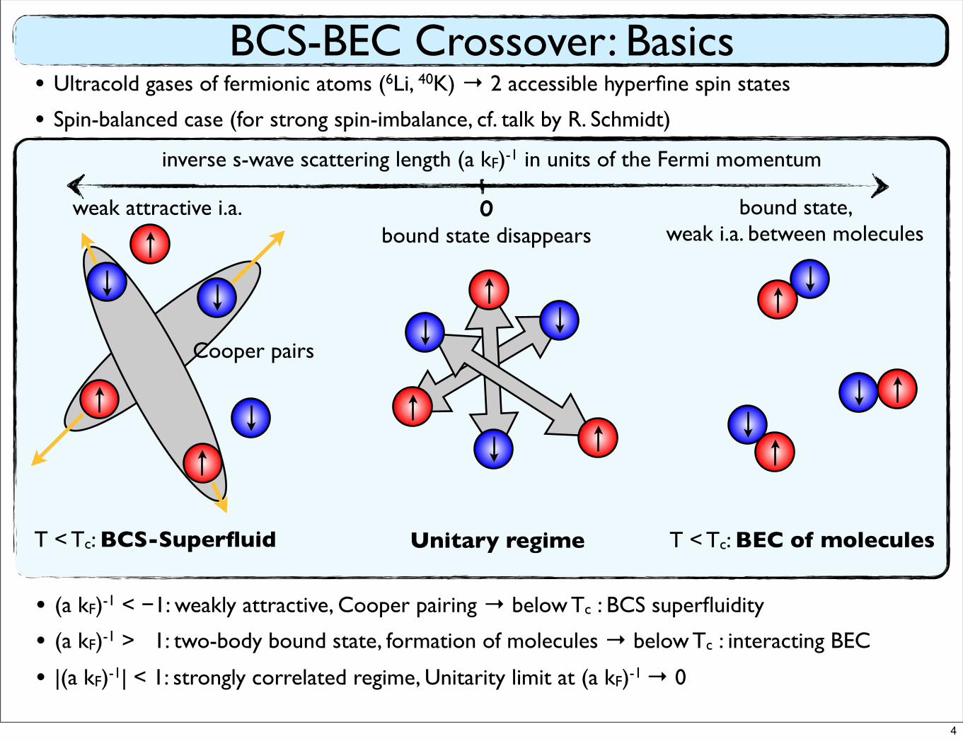
• (a kF)-1 < −1: weakly attractive, Cooper pairing → below Tc : BCS superfluidity

• (a kF)-1 > 1: two-body bound state, formation of molecules → below Tc : interacting BEC

• |(a kF)-1| < 1: strongly correlated regime, Unitarity limit at (a kF)-1 → 0

Cooper pairs

bound state, weak i.a. between molecules

weak attractive i.a. 0

inverse s-wave scattering length (a kF)-1 in units of the Fermi momentum

T < Tc: BCS-Superfluid T < Tc: BEC of moleculesUnitary regime

• Ultracold gases of fermionic atoms (6Li, 40K) → 2 accessible hyperfine spin states

• Spin-balanced case (for strong spin-imbalance, cf. talk by R. Schmidt)

bound state disappears

4

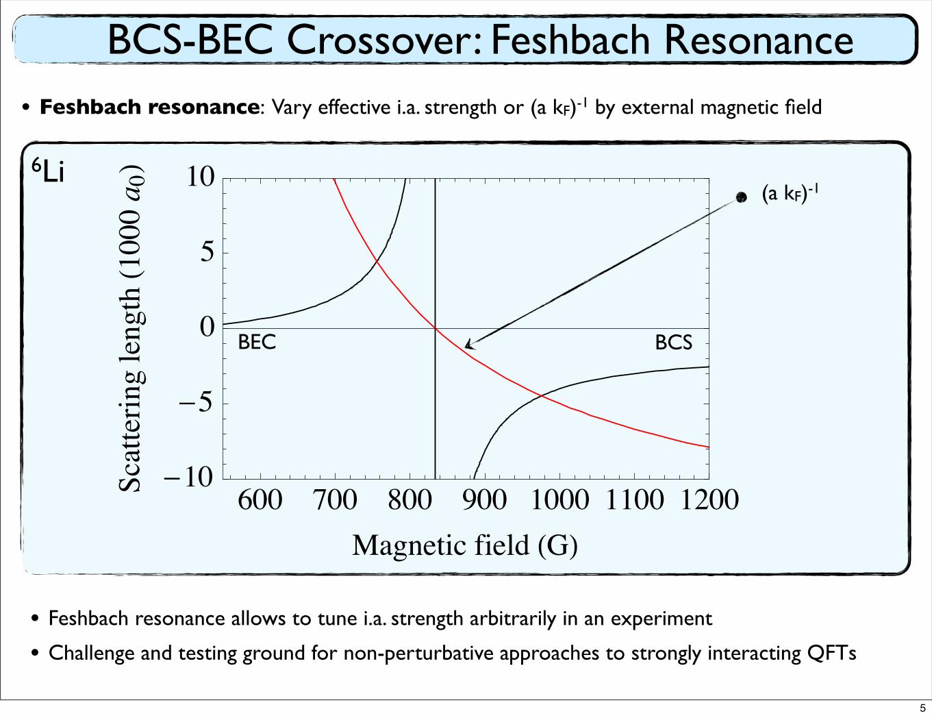
BCS-BEC Crossover: Feshbach Resonance• Feshbach resonance: Vary effective i.a. strength or (a kF)-1 by external magnetic field

• Feshbach resonance allows to tune i.a. strength arbitrarily in an experiment

• Challenge and testing ground for non-perturbative approaches to strongly interacting QFTs

BEC BCS

600 700 800 900 1000 1100 1200�10

�5

0

5

10

Magnetic field �G�Scatteringlength�1000

a 0�

(a kF)-1

6Li

5

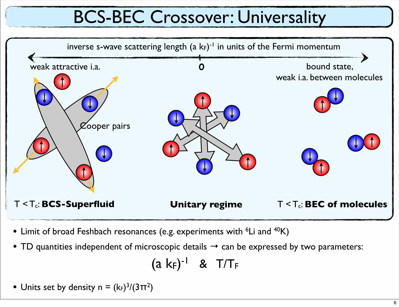
• Limit of broad Feshbach resonances (e.g. experiments with 6Li and 40K)

• TD quantities independent of microscopic details → can be expressed by two parameters:

• Units set by density n = (kF)3/(3π2)

(a kF)-1 & T/TF

BCS-BEC Crossover: Universality

Cooper pairs

bound state, weak i.a. between molecules

weak attractive i.a. 0

inverse s-wave scattering length (a kF)-1 in units of the Fermi momentum

T < Tc: BCS-Superfluid T < Tc: BEC of moleculesUnitary regime

6

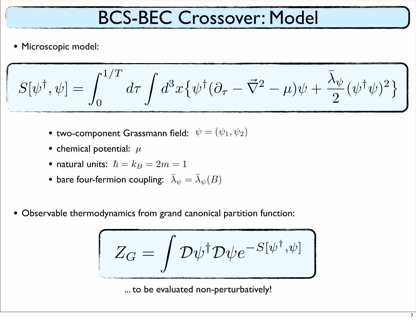
• Microscopic model:

• Observable thermodynamics from grand canonical partition function:

... to be evaluated non-perturbatively!

BCS-BEC Crossover: Model

• two-component Grassmann field:

• chemical potential:

• natural units:

• bare four-fermion coupling:

ψ = (ψ1,ψ2)

µ

� = kB = 2m = 1

S[ψ†,ψ] =

� 1/T

0dτ

�d3x

�ψ†(∂τ − �∇2 − µ)ψ +

λ̄ψ

2(ψ†ψ)2

�

λ̄ψ = λ̄ψ(B)

ZG =

�Dψ†Dψe−S[ψ†,ψ]

7

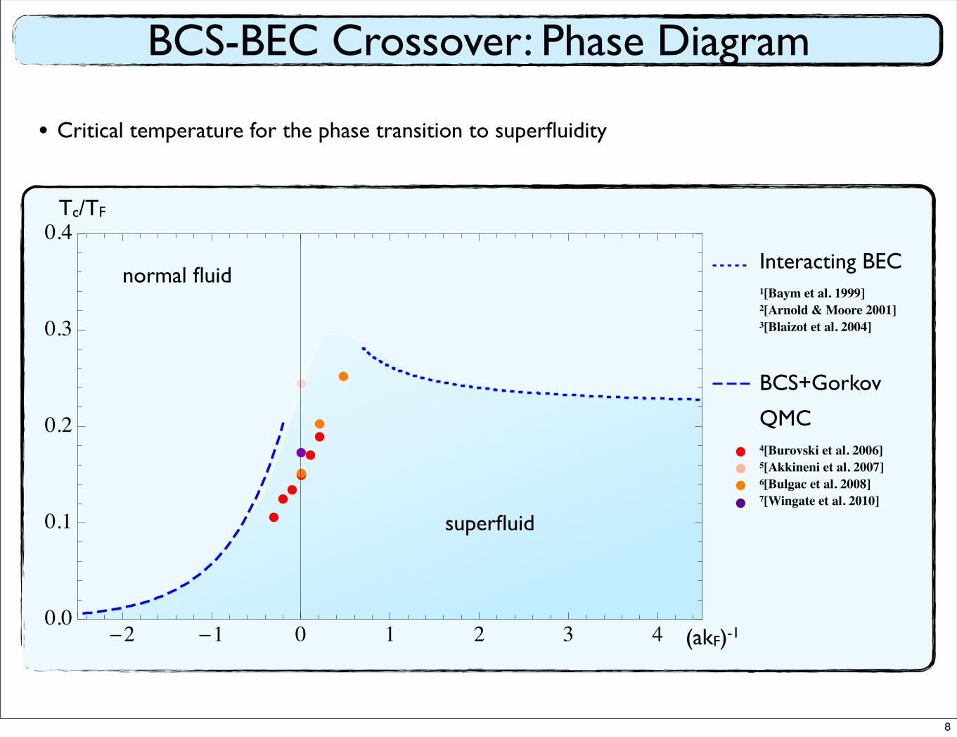
BCS-BEC Crossover: Phase Diagram

• Critical temperature for the phase transition to superfluidity

(akF)-1

Tc/TF

superfluid

normal fluidInteracting BEC1[Baym et al. 1999]2[Arnold & Moore 2001]3[Blaizot et al. 2004]

BCS+Gorkov

QMC4[Burovski et al. 2006]5[Akkineni et al. 2007]6[Bulgac et al. 2008]7[Wingate et al. 2010]

�2 �1 0 1 2 3 40.0

0.1

0.2

0.3

0.4

8

2. FRG Studies of the BCS-BEC Crossover

with Stefan Flörchinger, Sebastian Diehl, Holger Gies, Jan Pawlowski and Christof Wetterich

9

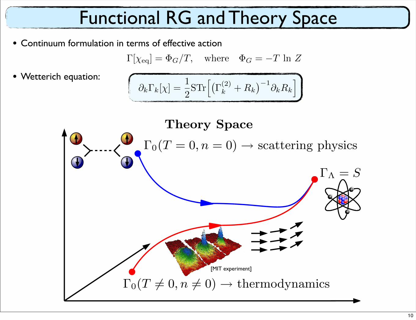
• Continuum formulation in terms of effective action

• Wetterich equation:

Functional RG and Theory Space

∂kΓk[χ] =1

2STr

��Γ(2)k +Rk

�−1∂kRk

�

Γ[χeq] = ΦG/T, where ΦG = −T ln Z

Theory Space

!0(T = 0, n = 0) ! scattering physics

!0(T "= 0, n "= 0) ! thermodynamics

!! = S

[MIT experiment]

10

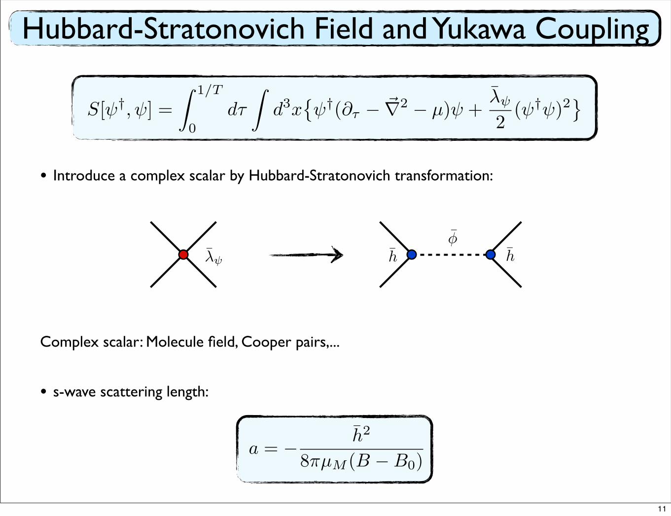
Hubbard-Stratonovich Field and Yukawa Coupling

• Introduce a complex scalar by Hubbard-Stratonovich transformation:

Complex scalar: Molecule field, Cooper pairs,...

• s-wave scattering length:

a = − h̄2

8πµM (B −B0)

S[ψ†,ψ] =

� 1/T

0dτ

�d3x

�ψ†(∂τ − �∇2 − µ)ψ +

λ̄ψ

2(ψ†ψ)2

�

λ̄ψ h̄ h̄φ̄

11

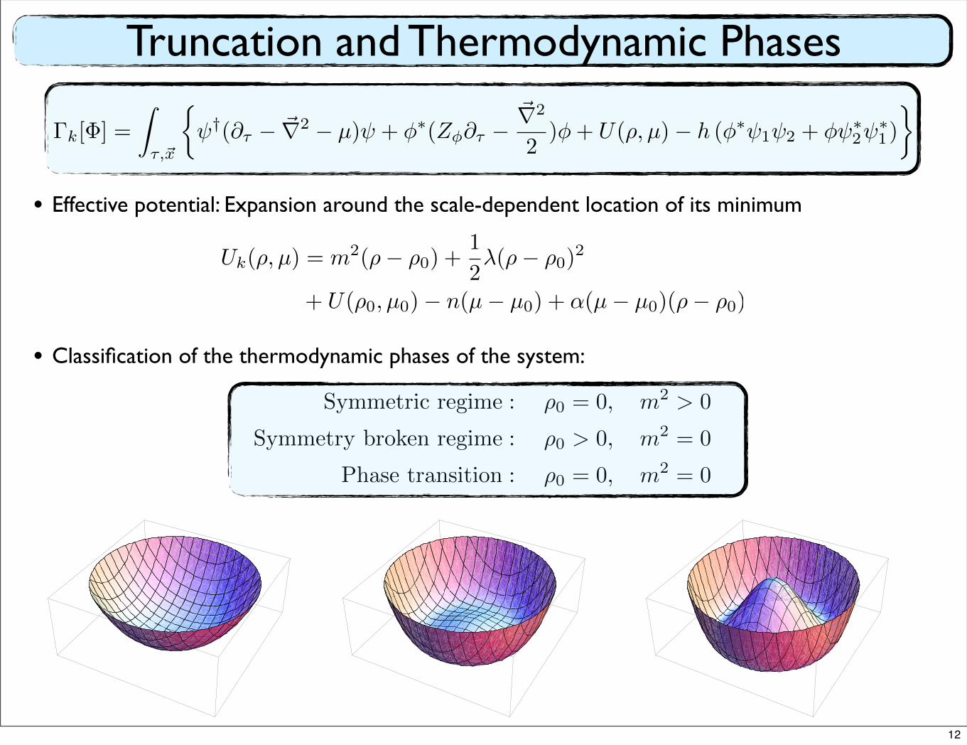
Truncation and Thermodynamic Phases

• Effective potential: Expansion around the scale-dependent location of its minimum

Uk(ρ, µ) = m2(ρ− ρ0) +1

2λ(ρ− ρ0)

2

+ U(ρ0, µ0)− n(µ− µ0) + α(µ− µ0)(ρ− ρ0)

• Classification of the thermodynamic phases of the system:

Symmetric regime : ρ0 = 0, m2 > 0

Symmetry broken regime : ρ0 > 0, m2 = 0

Phase transition : ρ0 = 0, m2 = 0

Γk[Φ] =

�

τ,�x

�ψ†(∂τ − �∇2 − µ)ψ + φ∗(Zφ∂τ −

�∇2

2)φ+ U(ρ, µ)− h (φ∗ψ1ψ2 + φψ∗

2ψ∗1)

�

12

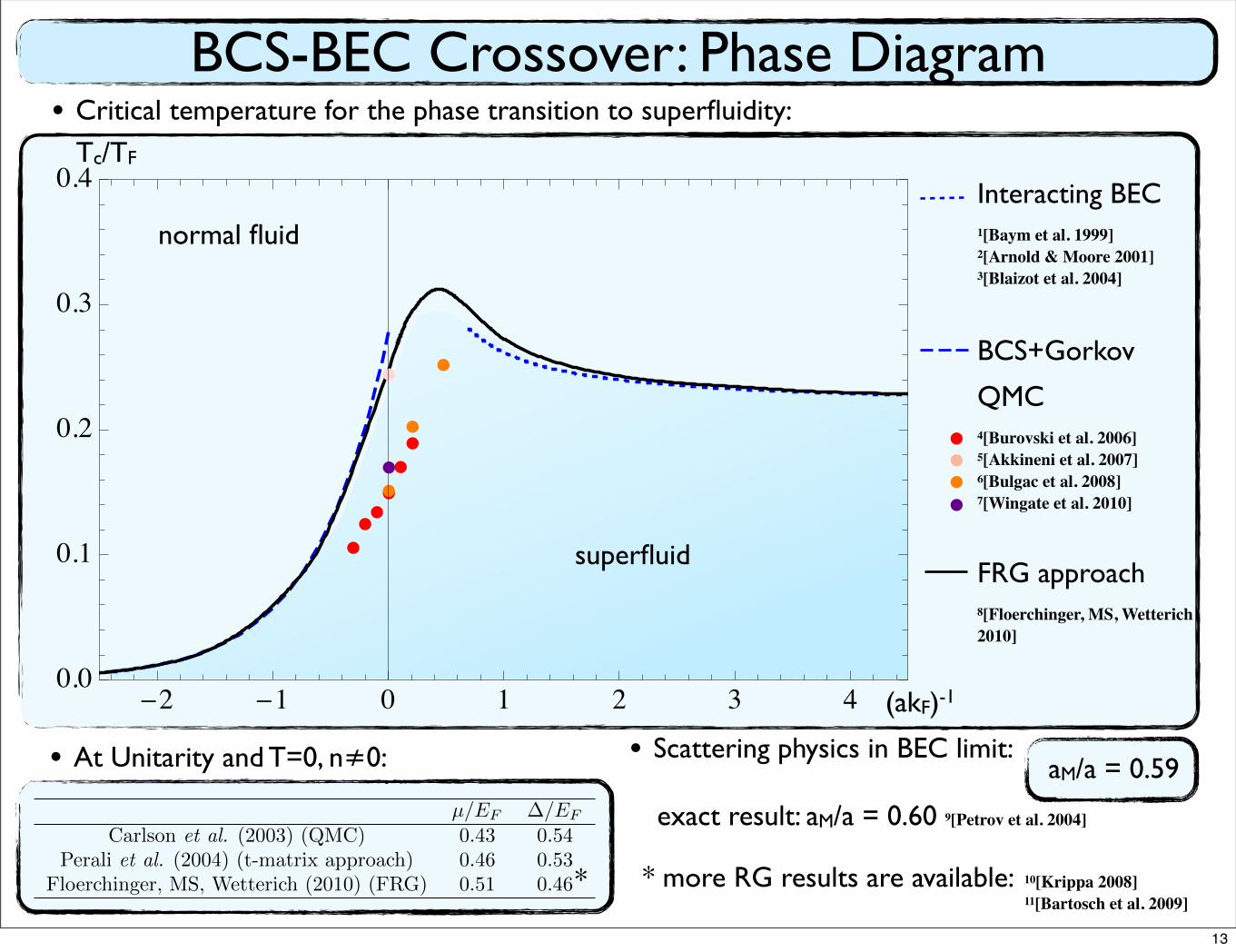
BCS-BEC Crossover: Phase Diagram• Critical temperature for the phase transition to superfluidity:

(akF)-1

Tc/TF

�2 �1 0 1 2 3 40.0

0.1

0.2

0.3

0.4

superfluid

normal fluid

• At Unitarity and T=0, n≠0: • Scattering physics in BEC limit:aM/a = 0.59

exact result: aM/a = 0.60 9[Petrov et al. 2004]

Interacting BEC1[Baym et al. 1999]2[Arnold & Moore 2001]3[Blaizot et al. 2004]

BCS+Gorkov

QMC4[Burovski et al. 2006]5[Akkineni et al. 2007]6[Bulgac et al. 2008]7[Wingate et al. 2010]

FRG approach8[Floerchinger, MS, Wetterich 2010]

10[Krippa 2008]11[Bartosch et al. 2009]

* * more RG results are available:

µ/EF ∆/EF

Carlson et al. (2003) (QMC) 0.43 0.54Perali et al. (2004) (t-matrix approach) 0.46 0.53

Floerchinger, MS, Wetterich (2010) (FRG) 0.51 0.46

13

3. Finite System Size Study

with Jens Braun and Sebastian Diehl

14

Motivation• Analysis of data from lattice simulations (performed in a finite volume)

• For unitary Fermi gas: Studies by MC community:

• Lattice studies:

• Limited range of system sizes

• Numerically expensive

• Cannot investigate transition between finite system and continuum limit

• FRG can! (recall talk by B. Klein)

Unitary regime

1[Wingate et al. 2009]2[Kaplan et al. 2010]3[Forbes et al. 2011]

15

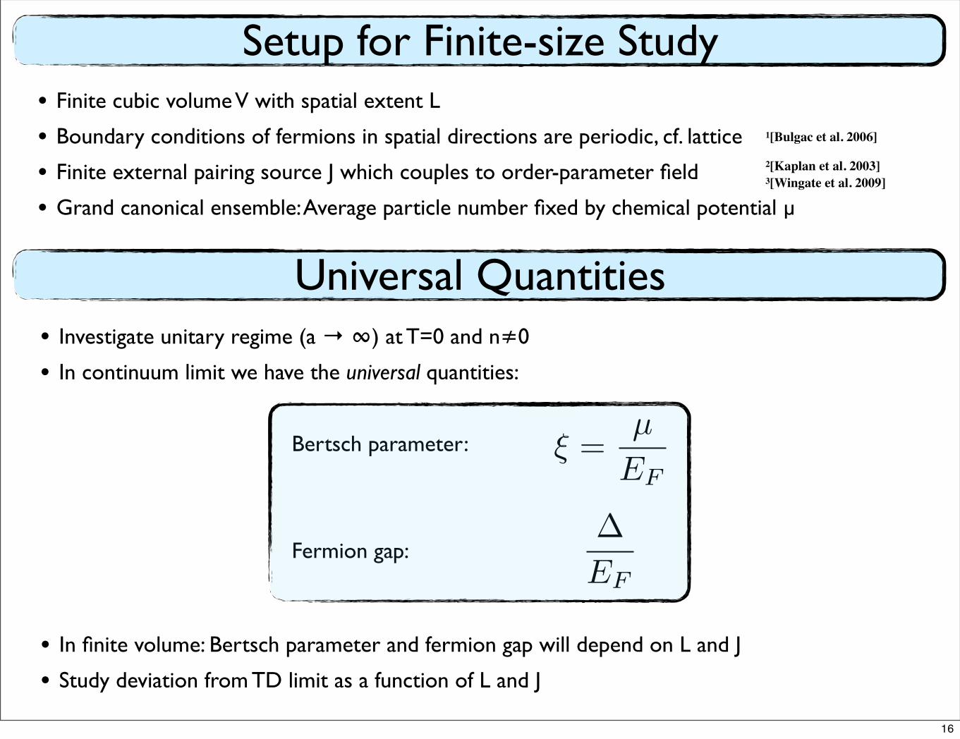
Setup for Finite-size Study• Finite cubic volume V with spatial extent L

• Boundary conditions of fermions in spatial directions are periodic, cf. lattice

• Finite external pairing source J which couples to order-parameter field

• Grand canonical ensemble: Average particle number fixed by chemical potential µ

• Investigate unitary regime (a → ∞) at T=0 and n≠0

• In continuum limit we have the universal quantities:

Bertsch parameter:

Fermion gap:

• In finite volume: Bertsch parameter and fermion gap will depend on L and J

• Study deviation from TD limit as a function of L and J

ξ =µ

EF

∆

EF

Universal Quantities

1[Bulgac et al. 2006]

2[Kaplan et al. 2003]3[Wingate et al. 2009]

16

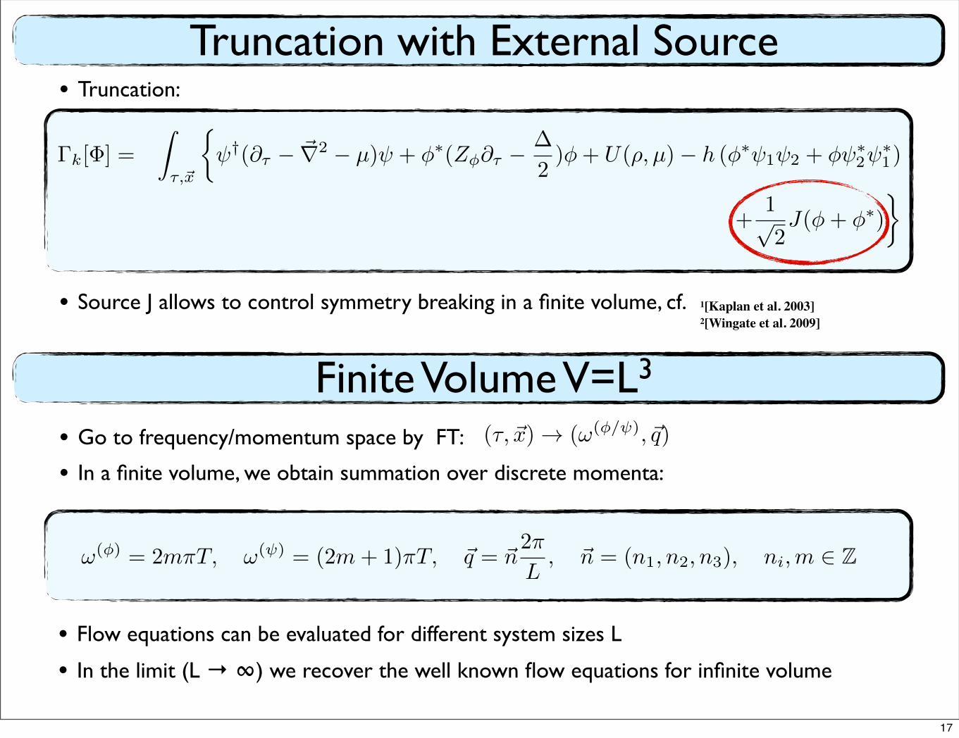
• Go to frequency/momentum space by FT:

• In a finite volume, we obtain summation over discrete momenta:

ω(φ) = 2mπT, ω(ψ) = (2m+ 1)πT, �q = �n2π

L, �n = (n1, n2, n3), ni,m ∈ Z

(τ, �x) → (ω(φ/ψ), �q)

• Flow equations can be evaluated for different system sizes L

• In the limit (L → ∞) we recover the well known flow equations for infinite volume

• Truncation:

Γk[Φ] =

�

τ,�x

�ψ†(∂τ − �∇2 − µ)ψ + φ∗(Zφ∂τ − ∆

2)φ+ U(ρ, µ)− h (φ∗ψ1ψ2 + φψ∗

2ψ∗1)

+1√2J(φ+ φ∗)

�

Finite Volume V=L3

Truncation with External Source

• Source J allows to control symmetry breaking in a finite volume, cf. 1[Kaplan et al. 2003]2[Wingate et al. 2009]

17

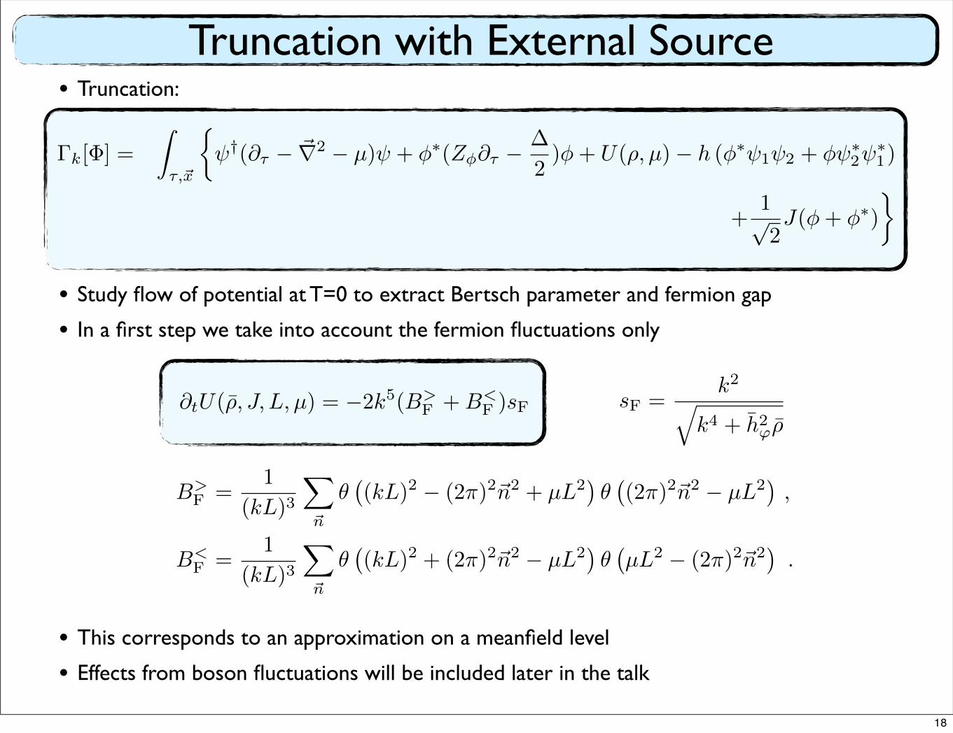
Truncation with External Source

• Study flow of potential at T=0 to extract Bertsch parameter and fermion gap

• In a first step we take into account the fermion fluctuations only

∂tU(ρ̄, J, L, µ) = −2k5(B>F +B<

F )sF sF =k2�

k4 + h̄2ϕρ̄

• Truncation:

B>F =

1

(kL)3

�

�n

θ�(kL)2 − (2π)2�n2 + µL2

�θ�(2π)2�n2 − µL2

�,

B<F =

1

(kL)3

�

�n

θ�(kL)2 + (2π)2�n2 − µL2

�θ�µL2 − (2π)2�n2

�.

• This corresponds to an approximation on a meanfield level

• Effects from boson fluctuations will be included later in the talk

Γk[Φ] =

�

τ,�x

�ψ†(∂τ − �∇2 − µ)ψ + φ∗(Zφ∂τ − ∆

2)φ+ U(ρ, µ)− h (φ∗ψ1ψ2 + φψ∗

2ψ∗1)

+1√2J(φ+ φ∗)

�

18

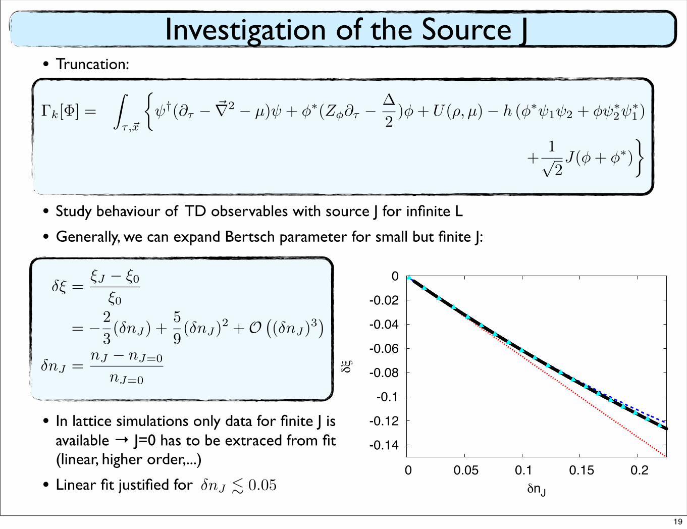
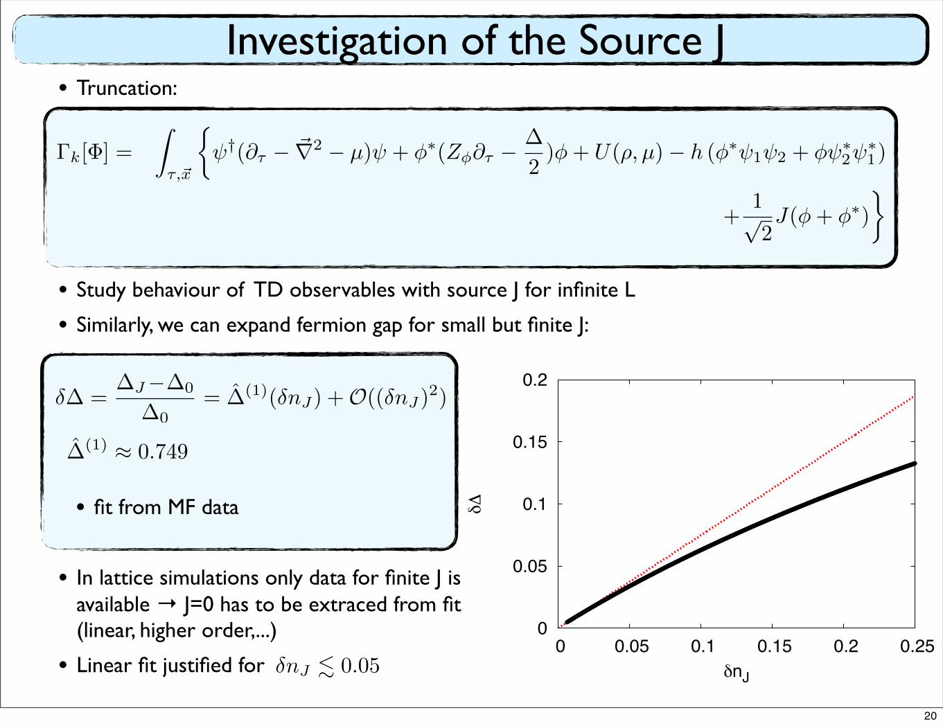
Investigation of the Source J• Truncation:

Γk[Φ] =

�

τ,�x

�ψ†(∂τ − �∇2 − µ)ψ + φ∗(Zφ∂τ − ∆

2)φ+ U(ρ, µ)− h (φ∗ψ1ψ2 + φψ∗

2ψ∗1)

+1√2J(φ+ φ∗)

�

• Study behaviour of TD observables with source J for infinite L

• Generally, we can expand Bertsch parameter for small but finite J:

-0.14

-0.12

-0.1

-0.08

-0.06

-0.04

-0.02

0

0 0.05 0.1 0.15 0.2nJ

• In lattice simulations only data for finite J is available → J=0 has to be extraced from fit (linear, higher order,...)

• Linear fit justified for

δξ =ξJ − ξ0

ξ0

= −2

3(δnJ) +

5

9(δnJ)

2 +O�(δnJ)

3�

δnJ =nJ − nJ=0

nJ=0

δnJ � 0.05

19

Investigation of the Source J• Truncation:

Γk[Φ] =

�

τ,�x

�ψ†(∂τ − �∇2 − µ)ψ + φ∗(Zφ∂τ − ∆

2)φ+ U(ρ, µ)− h (φ∗ψ1ψ2 + φψ∗

2ψ∗1)

+1√2J(φ+ φ∗)

�

• Study behaviour of TD observables with source J for infinite L

• Similarly, we can expand fermion gap for small but finite J:

• In lattice simulations only data for finite J is available → J=0 has to be extraced from fit (linear, higher order,...)

• Linear fit justified for δnJ � 0.05

0

0.05

0.1

0.15

0.2

0 0.05 0.1 0.15 0.2 0.25nJ

δ∆ =∆J−∆0

∆0= ∆̂(1)(δnJ) +O((δnJ)

2)

∆̂(1) ≈ 0.749

• fit from MF data

20

Finite Volume V=L3

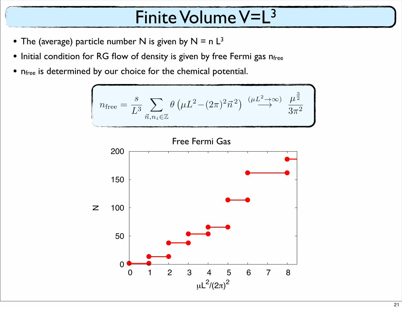
• The (average) particle number N is given by N = n L3

• Initial condition for RG flow of density is given by free Fermi gas nfree

• nfree is determined by our choice for the chemical potential.

nfree =s

L3

�

�n,ni∈Zθ�µL2−(2π)2�n 2

� (µL2→∞)−→ µ32

3π2

0

50

100

150

200

0 1 2 3 4 5 6 7 8

N

µL2/(2 )2

Free Fermi Gas

21

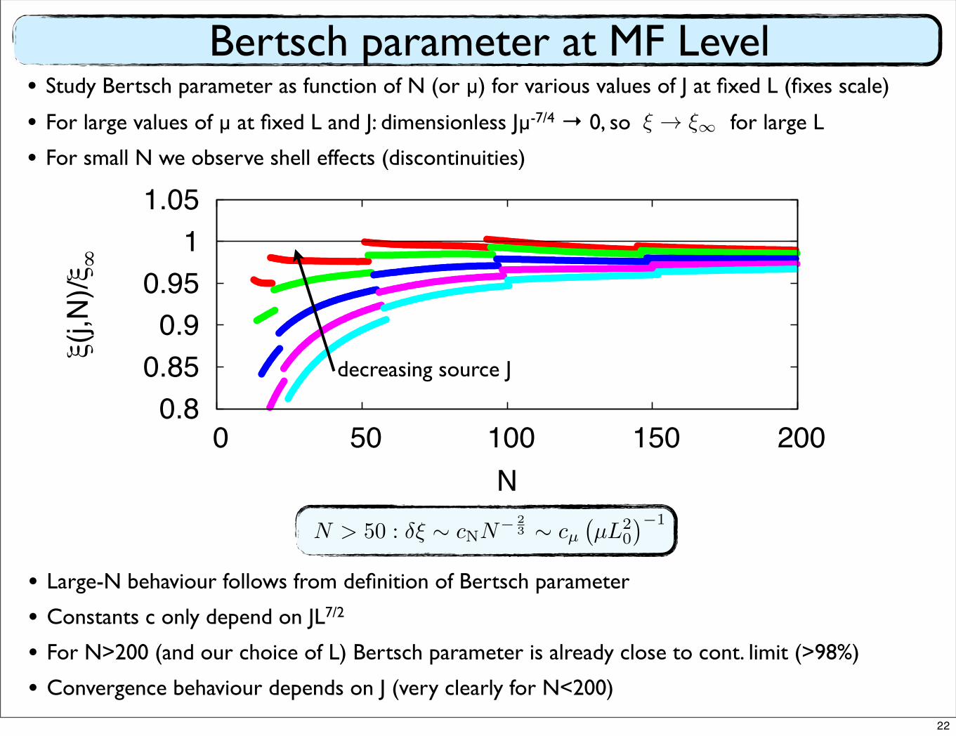
Bertsch parameter at MF Level• Study Bertsch parameter as function of N (or µ) for various values of J at fixed L (fixes scale)

• For large values of µ at fixed L and J: dimensionless Jµ-7/4 → 0, so for large L

• For small N we observe shell effects (discontinuities)

ξ → ξ∞

N > 50 : δξ ∼ cNN− 2

3 ∼ cµ�µL2

0

�−1

• Large-N behaviour follows from definition of Bertsch parameter

• Constants c only depend on JL7/2

• For N>200 (and our choice of L) Bertsch parameter is already close to cont. limit (>98%)

• Convergence behaviour depends on J (very clearly for N<200)

0.8 0.85

0.9 0.95

1 1.05

0 50 100 150 200

(j,N

)/

N

0.8 0.85

0.9 0.95

1 1.05

0 1 2 3 4 5

(j,!

L 02 )/

!L02/(2 )2

decreasing source J

22

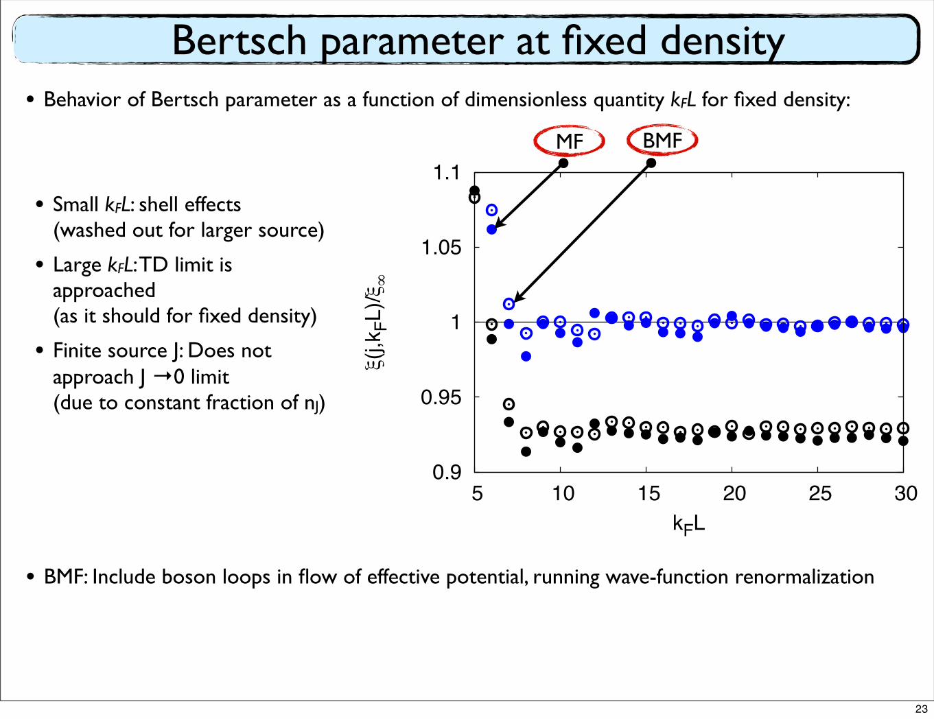
Bertsch parameter at fixed density

0.9

0.95

1

1.05

1.1

5 10 15 20 25 30

(j,k F

L)/

kFL

• Behavior of Bertsch parameter as a function of dimensionless quantity kFL for fixed density:

• Small kFL: shell effects(washed out for larger source)

• Large kFL: TD limit is approached (as it should for fixed density)

• Finite source J: Does not approach J →0 limit (due to constant fraction of nJ)

• BMF: Include boson loops in flow of effective potential, running wave-function renormalization

BMFMF

23

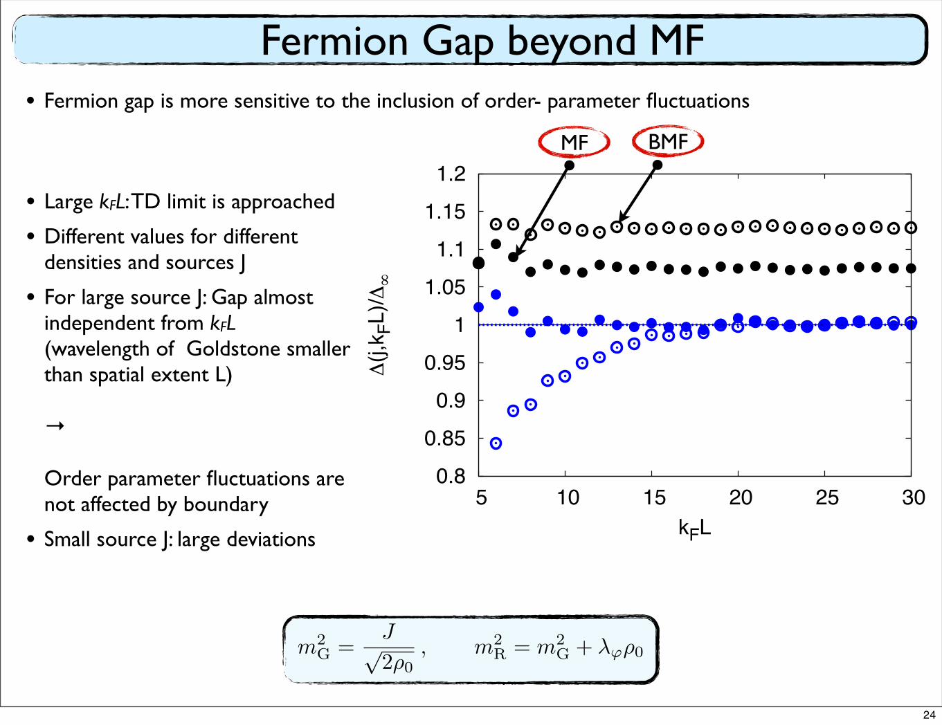
Fermion Gap beyond MF• Fermion gap is more sensitive to the inclusion of order- parameter fluctuations

• Large kFL: TD limit is approached

• Different values for different densities and sources J

• For large source J: Gap almost independent from kFL (wavelength of Goldstone smaller than spatial extent L)

→

Order parameter fluctuations are not affected by boundary

• Small source J: large deviations

0.8 0.85

0.9 0.95

1 1.05

1.1 1.15

1.2

5 10 15 20 25 30

(j,k F

L)/

kFL

BMFMF

m2G =

J√2ρ0

, m2R = m2

G + λϕρ0

24

Conclusions

• Finite size study of Tc(J,L)

& Outlook

• FRG connects BCS-/BEC-limits continuously with unitary regime and gives results with a reasonable accuracy throughout the whole crossover

• Using the FRG we have access to the shape of the volume and the particle number dependence of observables over a wide range of system sizes

• Volume-effects depend strongly on observable

• Improves understanding of convergence of finite volume systems, useful for MC simulations

25