finite element model of soil water and nutrient transport ...comte/pdf/article2.pdf · finite...

Finite element model of soil water and nutrient transport with root uptake:explicit geometry and unstructured adaptive meshing

Pierre-Henri Tournier · Frederic Hecht · Myriam Comte

Abstract In this paper, we consider a model of soil water and nutrient transport with plant root uptake. The ge-ometry of the plant root system is explicitly taken into account in the soil model. We first describe our modelingapproach. Then, we introduce an adaptive mesh refinement procedure enabling us to accurately capture the geom-etry of the root system and small-scale phenomena in the rhizosphere. Finally, we present a domain decompositiontechnique for solving the problems arising from the soil model as well as some numerical results.

Keywords finite element method; unstructured mesh adaptation; domain decomposition; plant root uptake

1 Introduction

Numerous models have been developed in the past in order to adress the different spatial and temporal scalesrelevant to soil water and nutrient transport and uptake by plant roots, from crop models used to predict yields at thefield level to recent plant based models involving the explicit architectural description of root system development.

Spatially explicit models defining 3D plant architecture are designed to investigate the relationship betweenroot architectural traits and the spatio-temporal variability of resource supply. They are providing insights forunderstanding various root-soil interactions over a range of spatial scales and aid in the design of agriculturalmanagement schemes for improving plant performance in specific environments.

However, simulation of water and nutrient uptake is challenging especially if we consider spatial hetero-geneities and local soil conditions in the rhizosphere around the roots, which are often quite different from thosein the bulk soil. In addition, the efficiency of yield enhancement techniques depends on responsive root growthwhich allows plants to forage with precision in an heterogeneous environment.

This work is an attempt to include and resolve accurately local rhizosphere processes occurring at the individ-ual root level in explicit plant scale models by taking advantage of the recent advances of scientific computing inthe field of adaptive meshing and parallel computing.

The mechanistic model described here can be used to investigate plant-soil relationships in specific situationsthrough for example sensitivity analysis, as well as verifying hypotheses and simplifications that are made in othermodels. Such applications will be the focus of subsequent papers.

The model is comparable to [7,11] where a discretization technique based on regular grids is employed. Insuch models, soil-root fluxes are taken into account in soil voxels by averaging and distributing between the soilnodes. In this work, we develop a new approach that takes advantage of the flexibility of adaptive refinementof unstructured finite element meshes to resolve small-scale behaviours such as the local hydraulic conductivitydrop near the soil-root interface while retaining the simplicity of the standard finite element method. Adaptiveunstructured volume remesh ing is quite a powerful tool when considering complex structures such as plant rootsystems.

P.-H. Tournier E-mail: [email protected] · F. Hecht E-mail: [email protected] ·M. Comte E-mail: [email protected] Pierre et Marie Curie - Paris 6, UMR 7598 Laboratoire Jacques-Louis Lions, Paris, F-75005 France

2 Pierre-Henri Tournier et al.

The paper is organized as follows: section 2 describes our water model. We consider that the root system canbe represented as a tree-like network composed of cylindrical root segments. We then define radial and axial waterflows on this network that can be coupled to the soil model via a sink term in the Richards equation. The sink termis constructed upon a characteristic function representative of the geometry of the root system. In section 3, thenutrient model is presented in a similar way. Section 4 briefly describes the standard finite element method used inthis work. In section 5, the adaptive mesh refinement algorithm is presented: the characteristic function of the rootsystem is computed and then used to construct a metric field in order to drive the mesh adaptation procedure. Sincesuch an approach is computationally intensive, a parallelization technique based on a scalable Schwarz domaindecomposition method is used to solve the problems arising from the soil and nutrient models. The procedure ishighlighted in section 6.

Throughout this paper the soil domain is denoted by Ω ⊂Rd(d = 2,3). We consider the evolution of the waterpotential and nutrient concentration for t ∈ [0,T ],T > 0.

2 The water model

2.1 The Richards equation

In soils, water movement is governed by the Richards equation. Richards equation is derived from the continuityequation

∂θ

∂ t+∇.q = S, (2.1)

with θ the volumetric water content, q the macroscopic Darcy flow and S representing sources/sinks.Darcy law relates the water flow to the pressure of the water at any time t:

q =−K∇H, (2.2)

where K is the hydraulic conductivity and H is the total hydraulic head (water potential on weight basis), whichcan be expressed as

H = h+ z. (2.3)

Here, h is the pressure head and comes from a hydrostatic pressure if h > 0 and from a capillary pressure if h < 0.z is the height against the gravitational direction.

The volumetric water content θ and the hydraulic conductivity K are linked to the pressure head h by relationshipsthat depend on the soil properties.

By combining (2.1) and (2.2) we obtain the Richards equation:

∂t(θ(h))−∇.(K(h)∇(h+ z)) = S in [0,T ]×Ω . (2.4)

Equation (2.4) is subject to the initial condition

h(x,0) = h0(x) in Ω , (2.5)

and the no-flux boundary condition

K(h)∇(h+ z).n = 0 on [0,T ]×∂Ω , (2.6)

where n denotes the unit outward normal to the boundary of the domain Ω .

The θ(h) and K(h) relationships are given by empirical models whose parameters depend on the soil physicalproperties. We use the Brooks-Corey model:

Θ(h) :=θ(h)−θm

θM−θm=

[hhb

]−λ

:=

(hhb

)−λ

for h≤ hb

1 for h≥ hb,

K(h) = Ks

[hhb

]−λe(λ )

with e(λ ) := 3+2λ,

(2.7)

Finite element model of soil water and nutrient transport with root uptake: explicit geometry and unstructured adaptive meshing 3

where Θ is the normalized water content.The parameters of the model are defined as follows:

– θM is the saturated water content.– θm is the residual water content.– Ks is the saturated hydraulic conductivity.– hb is the bubbling pressure head.– λ is the pore size distribution index.

Experimental evidence has shown that a cycle of wetting-drying of a soil exhibits hysteresis: the water contenthas different profiles with respect to the wetting and draining processes. This effect can be of importance whenconsidering irrigation or rainfall together with root water uptake. Although hysteresis effects are neglected in themodel described here, hysteresis in the soil water retention function θ(h) can be taken into account by includingempirical hysteresis models such as [16] based on main wetting and drying curves.

We introduce the Kirchhoff transformation κ which enables us to reduce the nonlinearity of Richards equation:

κ : h→ p∫ h

0K(p)d p. (2.8)

The new variable p is called the generalized pressure. Previous applications of the Kirchhoff transformation toRichards equation can be found for example in [20,25,12,23].The water content as a function of p is denoted by

M(p) := θ(κ−1(p)). (2.9)

Using the chain rule, we have

∇p = K(h)∇(h). (2.10)

Thus the Richards equation reads:

∂t(M(p))−∇.(∇p+K(κ−1(p))∇z)−S = 0 in [0,T ]×Ω . (2.11)

The transformed equation is a semilinear equation in which the nonlinearity in front of the spatial derivative hasbeen eliminated.

Using the backward Euler scheme for the time discretization, we are able to write the following weak formu-lation of the semi-discrete problem: find pn+1 ∈ H1(Ω) such that ∀v ∈ H1(Ω),

∫Ω

M(pn+1)−M(pn)

∆ tv+

∫Ω

∇pn+1∇v+

∫Ω

K(κ−1(pn+1))∇z∇v−∫

Ω

Sv = 0. (2.12)

Following the approach suggested in [4,23], the solution at each time step is obtained iteratively; applying New-ton’s method to linearize M(pn+1) gives the following Newton-like iteration where i is the inner iteration counterfor time n+1:

∫Ω

M′(pi)(pi+1− pi)+M(pi)−M(pn)

∆ tv+

∫Ω

∇pi+1∇v+

∫Ω

K(κ−1(pi))∇z∇v−∫

Ω

Sv = 0. (2.13)

In practice, as the soil dries the capillary effects get stronger as well as the nonlinearities, while the gravity termbecomes of less importance. This allows us to use a simple picard method for the gravity term with no effect onthe convergence rate.

The use of the Brooks-Corey model allows us to express the Kirchhoff transformation and its inverse and thetransformed functions involved in (2.13) explicitly in a closed form as in [3]:


p = κ(h) =

hb

−λe(λ )+1

(hhb

)−λe(λ )+1+ −λe(λ )hb−λe(λ )+1 for h≤ hb

h for h≥ hb,

h = κ−1(p) =

hb

(p(−λe(λ )+1)

hb+λe(λ )

) 1−λe(λ )+1 for pc < p≤ hb

p for p≥ hb,

M(p) =

θm +(θM−θm)(

p(−λe(λ )+1)hb

+λe(λ )) λ

λe(λ )−1 for pc < p≤ hb

θM for p≥ hb,

M′(p) =

(θM−θm)−λ

hb

(p(−λe(λ )+1)

hb+λe(λ )

) λ

λe(λ )−1−1for pc < p≤ hb

0 for p≥ hb,

K(κ−1(p)) =

(

p(−λe(λ )+1)hb

+λe(λ )) λe(λ )

λe(λ )−1 for pc < p≤ hb

1 for p≥ hb,

(2.14)

Since the transformations (2.14) are obtained analytically, the additional computational cost of employing theKirchhoff transformation is negligible compared to that of solving the linear system arising from the discretizationof (2.13).

Note that the discontinuity of M′(p) for p = hb comes from the non-differentiability of the Brooks-Coreyfunction θ(h) at h = hb. However, we do not consider the saturated case h≥ hb in the examples presented in thispaper. Besides, from a numerical point of view, numerical tests have shown that for realistic parameter values thediscontinuity is small and does not hinder the convergence of the iterative method.

2.2 Root water uptake

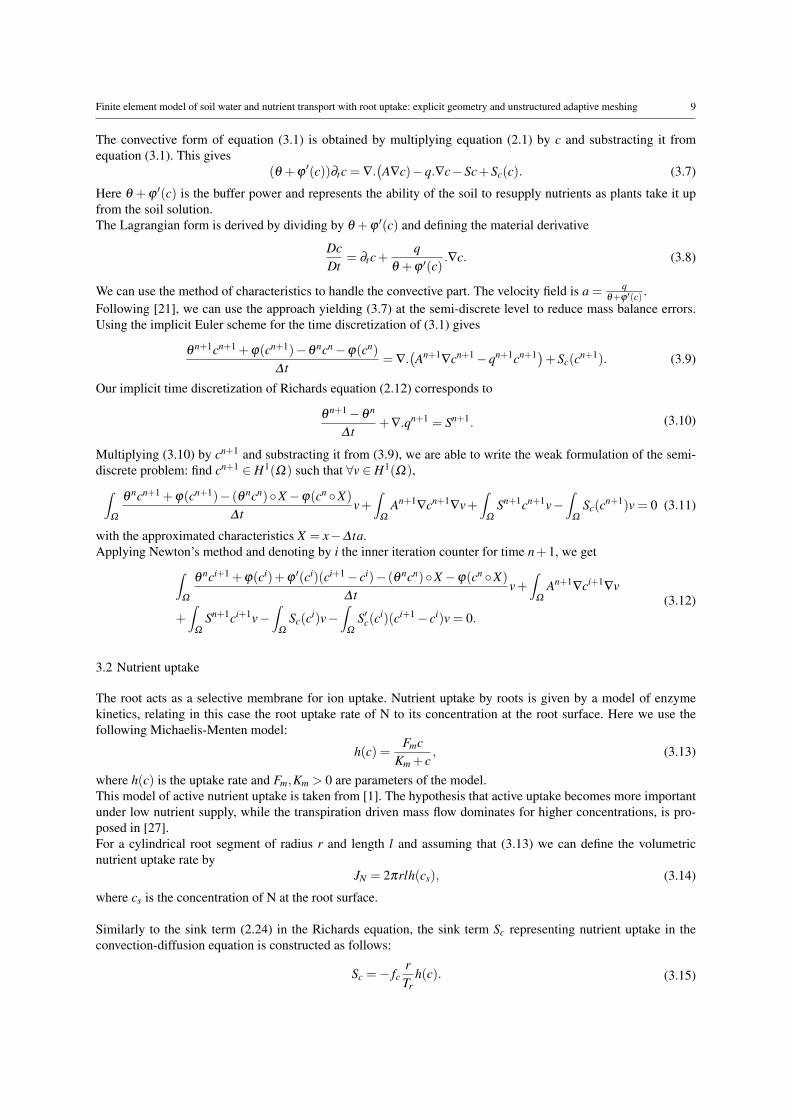
Here we consider that the root system is composed of cylindrical root segments. It can then be represented as aseries of interconnected nodes forming a network of segments Σ , each segment with its own parameters (radius,conductivity, etc.). Such a representation can be generated by the Matlab code RootBox [18], which implementsa root system growth model based on L-Systems. RootBox is a root architectural model that explicitly simulatesthe architecture of root systems in the 3D space, using a set of growth rules which are applied to a series of roottypes or classes, with each root type having its own characteristic set of growth parameters such as root elongationrate or branching density. The algorithm computes elongation and branching of the roots according to the initialgrowth speed, lengths of apical and basal zones as well as internodal distances, maximal number of branches andbranching angles. Growth direction can follow different types of user defined tropisms. The model has a stochasticcomponent in that all parameters can be given with mean and standard deviation. Fig. 1 shows an example of amaize root system generated by RootBox.

In the following we define water flows on the root network and describe the coupling with the soil model aswas done in [7].

We make the same assumptions as in [7], which are explained in [6]. The model describing root water uptakecan be found in [8,17]: water flow in roots and between soil and roots is described by the transpiration-cohesion-tension mechanism and follows an Ohm’s law analogy.Let us recall the hypotheses made in [6]: First, the influence of solutes on flow is neglected, because duringperiods of active transpiration, the hydrostatic pressure gradient rather than the osmotic potential gradient is theeffective driving force for flow. The second hypothesis consists in neglecting the capacitive effect of the rootsand considering only steady-state flow, because water stored in roots is generally small compared to transpirationrequirements. Thus, for a cylindrical root segment of radius r and length l and following [17], we can define thevolumetric radial water flow into the root from the soil Jr and the longitudinal flow up the root in the xylem Jx as

Jr = Lrsr(hs−hr),

Jx =−Krdhr

dl,

(2.15)

Finite element model of soil water and nutrient transport with root uptake: explicit geometry and unstructured adaptive meshing 5.. 1D representation of the root system

The root system geometryis represented as a seriesof interconnected nodes,forming a network of rootsegments.

In this example, a codedeveloped at BOKU is usedthat simulates the growthof the root system of a20-days-old maize plant andoutputs the correspondinggeometry.

Pierre-Henri Tournier Soil water movement and water uptake by the root system of a maize plant

Fig. 1 Example of a 20-days-old maize root system generated by RootBox composed of 10611 segments

where

– Lr is the radial conductivity of the root and represents the conductivity of the series of tissues from the rootsurface to the xylem,

– Kr is the xylem conductance,– sr = 2πrl is the root-soil interface area,– hs is the soil water potential at the root surface,– hr is the water potential in the xylem.

Although these simplifications are made in our model as well, the model can be extended by taking into accountosmotic gradients and capacitive effects of roots.

Equations (2.15) giving radial and longitudinal flows can be used to formulate a water mass balance equationfor a given root node i of parent node p in the tree-like structure as depicted in Fig. 2:

Jx,i = ∑j∈childs(i)

Jx, j + Jr,i, (2.16)

which can be written as

−Kr,ihr,p−hr,i

li=− ∑

j∈childs(i)

(Kr, j

hr,i−hr, j

l j

)+Lr,i2πrili

(hs,i−hr,i)+(hs,p−hr,p)

2. (2.17)

Here Kr,i,Lr,i,ri and li refer to the root segment (p, i) while Kr, j and l j relate to the root segment (i, j). hs,i and hr,iare the soil water potential at root node i and the xylem water potential at root node i respectively. We approximatethe potentials hs and hr for segment (i, p) by averaging their value at the two nodes i and p. Parameters Lr and Krare given for each segment and can depend on various data such as root type and age.

Writing (2.17) for every node in the tree-like structure, the xylem water potential vector (hr,i)i is then solutionof a linear system, with the right-hand side containing the soil factors represented by the hs,i.At the root collar, we can prescribe the transpiration flow or the xylem potential with a Neumann or Dirichletboundary condition respectively. We can follow the same approach as in [7,11]: In the case of a flux-type bound-ary condition, stress may occur when the evaporative demand cannot be met by the soil. In such a case, a maximum


p

i

j1 j2

Jx, j1 Jx, j2

Jx,i

Jr,i

Fig. 2 Water mass balance for root node i

allowable threshold value for absolute collar water potential is defined (usually taken as a typical value of the per-manent wilting point hw = −150 m), beyond which the collar boundary condition is switched from a flux-type(Neumann) to a pressure-head-type (Dirichlet) condition.Other models could also be considered, such as [24] where stomatal response to a drying soil is modeled by alogistic function with empirically determined parameters.

In order to take the radial water uptake flows into account in the soil water model, a sink term S in the Richardsequation is defined in the domain. Since the sink term represents root uptake flows in the 3D (or 2D) space, weconstruct S through a characteristic function of the root system fc representative of its geometry using the distancefunction to the root network Σ . The characteristic function fc can be seen as a smooth approximation of the 1Droot network Σ , taking the values 1 at the root and 0 away from the root, with a smooth change of width ε inbetween.The purpose of the characteristic function is threefold: define a regularization of the delta function representingthe network of segments Σ , construct a sink term matching the volume occupied by the roots by using the diameterof the root as the width of the regularization, and drive the adaptive mesh refinement procedure.

The function fc representative of the geometry of the root system in the domain is constructed as follows:

– For a point x of the domain Ω the distance d from x to the root is computed:

d(x) = mins∈Σ

ds(x), (2.18)

with Σ the set of root segments in the tree-like network. For each root segment s, the distance ds(x) from thepoint x to the segment s is easily computed using distance from line and point routines.

– The distance function d is then used to compute the characteristic function. There is a variety of admissibletransformations that we can use, and we choose the following:

fc(x) = fd (d(x)) = 1− tanh(

6d(x)ε

). (2.19)

We can choose ε to be equal to the radius of the root.

We can now build the sink term in the Richards equation. In order to ensure that the sink term in the soil modelcorresponds to the volumetric radial flow in the network model, we need to introduce a scale factor depending onthe choice of fd .

Let us consider the case of a cylindrical root segment s, formed by the nodes i and j. The corresponding radialflow is

Jr = Lr2πrrlr(hs,i−hr,i)+(hs, j−hr, j)

2. (2.20)

We want the integral of the corresponding sink term S over the domain to be equal to the outflow rate, i.e.∫Ω

S =−Jr. (2.21)


If fc is the characteristic function of the single root segment as defined above, using cylindrical coordinates we get(in the 3D case) ∫

Ω

fc ' 2πlr∫ R

0r fd(r)dr (2.22)

with R >> ε . The approximation error coming from the truncature in the integral is negligible for usual choicesof fd .Let us define Tr as

Tr =∫ R

0r fd(r)dr. (2.23)

We then define the sink term S as

S =− fcLrrr

Trhl , (2.24)

where hl only depends on the longitudinal coordinate and linearly interpolates hs−hr along the segment.Thus, we have ∫

Ω

S =−∫

Ω

fcLrrr

Trhl =−Lr2πrrlr

(hs,i−hr,i)+(hs, j−hr, j)

2=−Jr. (2.25)

The extension to the whole root system is straightforward.

Since the characteristic function does not correspond to an arrangement of perfect cylindrical root segmentsdue to its shape at root tips or in-between root segments, a modified approach consists in adjusting the surfaceareas of the root segments in the definition of the radial uptake flows in the root network model so that for eachroot segment, the volumetric uptake flow is equal to the actual contribution of the segment to the global sink termin the soil model. This approach ensures that the amount of water depleted in the soil water model is equal to thetranspiration rate in the network model, although the difference is minimal in actual computations.

The coupling between the tree-like model and the soil water model consists in iteratively solving the twoproblems until convergence. Let hti

s be the soil matric potential distribution at time ti, hks and hk

r the soil and xylemmatric potentials at inner iteration k and time ti+1. The coupling algorithm reads as follows:

1. h0s = hti

s .2. Solve the linear system of the tree-like model derived from (2.17) with soil factors hk

s , obtain hkr on the root

network.3. Compute the sink term S as in (2.24) using hk

s and hkr .

4. Perform an inner iteration of (2.13), obtain hs in the soil domain.5. hk+1

s = hks +αk(hs−hk

s), where αk is an under-relaxation parameter that ensures convergence of the system.6. If ||hs−hk

s ||> τ , go to 2. with k← k+1.

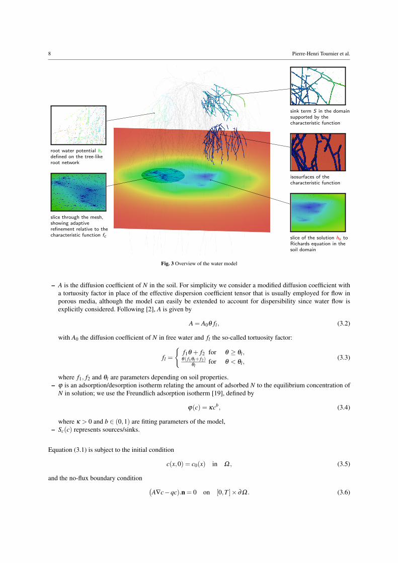
Fig. 3 gives an overview of the water model through an example.

3 The nutrient model

Here we consider the evolution of the concentration c of a nutrient ion N in the soil solution, governed by diffusion,mass flow, adsorption in the soil solid phase and root uptake.

3.1 The convection-diffusion equation

The convection-diffusion equation expresses the nutrient mass balance and can be written in its conservative form:

∂t(θc+ϕ(c)) = ∇.(A∇c−qc)+Sc(c) in [0,T ]×Ω , (3.1)

where


root water potential hrdefined on the tree-likeroot network

slice through the mesh,showing adaptiverefinement relative to thecharacteristic function fc

sink term S in the domainsupported by thecharacteristic function

isosurfaces of thecharacteristic function

slice of the solution hs toRichards equation in thesoil domain

Fig. 3 Overview of the water model

– A is the diffusion coefficient of N in the soil. For simplicity we consider a modified diffusion coefficient witha tortuosity factor in place of the effective dispersion coefficient tensor that is usually employed for flow inporous media, although the model can easily be extended to account for dispersibility since water flow isexplicitly considered. Following [2], A is given by

A = A0θ fl , (3.2)

with A0 the diffusion coefficient of N in free water and fl the so-called tortuosity factor:

fl =

f1θ + f2 for θ ≥ θl ,

θ( f1θl+ f2)θl

for θ < θl ,(3.3)

where f1, f2 and θl are parameters depending on soil properties.– ϕ is an adsorption/desorption isotherm relating the amount of adsorbed N to the equilibrium concentration of

N in solution; we use the Freundlich adsorption isotherm [19], defined by

ϕ(c) = κcb, (3.4)

where κ > 0 and b ∈ (0,1) are fitting parameters of the model,– Sc(c) represents sources/sinks.

Equation (3.1) is subject to the initial condition

c(x,0) = c0(x) in Ω , (3.5)

and the no-flux boundary condition (A∇c−qc).n = 0 on [0,T ]×∂Ω . (3.6)


The convective form of equation (3.1) is obtained by multiplying equation (2.1) by c and substracting it fromequation (3.1). This gives

(θ +ϕ′(c))∂tc = ∇.

(A∇c)−q.∇c−Sc+Sc(c). (3.7)

Here θ +ϕ ′(c) is the buffer power and represents the ability of the soil to resupply nutrients as plants take it upfrom the soil solution.The Lagrangian form is derived by dividing by θ +ϕ ′(c) and defining the material derivative

DcDt

= ∂tc+q

θ +ϕ ′(c).∇c. (3.8)

We can use the method of characteristics to handle the convective part. The velocity field is a = qθ+ϕ ′(c) .

Following [21], we can use the approach yielding (3.7) at the semi-discrete level to reduce mass balance errors.Using the implicit Euler scheme for the time discretization of (3.1) gives

θ n+1cn+1 +ϕ(cn+1)−θ ncn−ϕ(cn)

∆ t= ∇.

(An+1

∇cn+1−qn+1cn+1)+Sc(cn+1). (3.9)

Our implicit time discretization of Richards equation (2.12) corresponds to

θ n+1−θ n

∆ t+∇.qn+1 = Sn+1. (3.10)

Multiplying (3.10) by cn+1 and substracting it from (3.9), we are able to write the weak formulation of the semi-discrete problem: find cn+1 ∈ H1(Ω) such that ∀v ∈ H1(Ω),∫

Ω

θ ncn+1 +ϕ(cn+1)− (θ ncn)X−ϕ(cn X)

∆ tv+

∫Ω

An+1∇cn+1

∇v+∫

Ω

Sn+1cn+1v−∫

Ω

Sc(cn+1)v = 0 (3.11)

with the approximated characteristics X = x−∆ ta.Applying Newton’s method and denoting by i the inner iteration counter for time n+1, we get∫

Ω

θ nci+1 +ϕ(ci)+ϕ ′(ci)(ci+1− ci)− (θ ncn)X−ϕ(cn X)

∆ tv+

∫Ω

An+1∇ci+1

∇v

+∫

Ω

Sn+1ci+1v−∫

Ω

Sc(ci)v−∫

Ω

S′c(ci)(ci+1− ci)v = 0.

(3.12)

3.2 Nutrient uptake

The root acts as a selective membrane for ion uptake. Nutrient uptake by roots is given by a model of enzymekinetics, relating in this case the root uptake rate of N to its concentration at the root surface. Here we use thefollowing Michaelis-Menten model:

h(c) =Fmc

Km + c, (3.13)

where h(c) is the uptake rate and Fm,Km > 0 are parameters of the model.This model of active nutrient uptake is taken from [1]. The hypothesis that active uptake becomes more importantunder low nutrient supply, while the transpiration driven mass flow dominates for higher concentrations, is pro-posed in [27].For a cylindrical root segment of radius r and length l and assuming that (3.13) we can define the volumetricnutrient uptake rate by

JN = 2πrlh(cs), (3.14)

where cs is the concentration of N at the root surface.

Similarly to the sink term (2.24) in the Richards equation, the sink term Sc representing nutrient uptake in theconvection-diffusion equation is constructed as follows:

Sc =− fcrTr

h(c). (3.15)


The model can easily be adapted to implement other nutrient uptake models. For example, in [22,10] the soluteuptake term is defined as

S′(c) = εSc+(1− ε)Sc(c),

where ε ∈ [0,1] is a coefficient partitioning total uptake between passive uptake Sc where solute enters the root dis-solved in water and active uptake Sc(c), which could also be described following for example [15] by a Michaelis-Menten-type kinetic with a linear component.

4 Finite element formulation

In this section we describe briefly the Galerkin P1 finite element approximation of problems (2.13) and (3.12).Let Th be a mesh of the domain Ω . Let

Vh =

uh ∈ H1(Ω)∣∣∣ uh|K ∈ P1, ∀K ∈ Th

. (4.1)

Spatial discretization of Equation (2.13) leads to the following discrete variational problem: find ph ∈Vh such that∀vh ∈Vh, (

M′(pih)ph,vh

)+∆ t (∇ph,∇vh) =

(M′(pi

h)pih,vh

)−(M(pi

h),vh)+(M(pn

h),vh)

−(K(κ−1(pi

h))∇z,∇vh)+(Si

h,vh).

(4.2)

Spatial discretization of Equation (3.12) leads to the following discrete variational problem: find ch ∈Vh such that∀vh ∈Vh,

(θ nh ch,vh)+

(ϕ′(ci

h)ch,vh)+(An+1

h ∇ch,∇vh)+∆ t

(Sn+1

h ch,vh)−∆ t

(S′c(c

i)hch,vh)

=−(ϕ(ci

h),vh)+(ϕ′(ci

h)cih,vh

)+((θ n

h cnh)X ,vh)+(ϕ(cn

h X),vh)+∆ t(Sc(ci)h,vh

)−∆ t

(S′c(c

i)hcih,vh

).

(4.3)Numerical resolution of systems (4.2) and (4.3) is carried out using the finite element software FreeFem++ [9].

5 Mesh adaptation

The soil domain Ω is first represented by a regular initial simplicial finite element mesh. Since the characteristicfunction of the root system fc is poorly represented on the initial mesh, we refine it iteratively using anisotropicmesh adaptation. Since we expect high gradients and small-scale phenomena to be localized near the roots (i.e.where fc exhibits strong variations), this type of a priori refinement is adequate.The main steps of the adaptive procedure are as follows: First, we compute fc for each node of the mesh. Then wedefine a nodal based anisotropic metric from the Hessian of the function fc. Finally, the mesh is adapted using thesize and streching of elements provided by the metric. This procedure is repeated iteratively.In 2D, we use the built-in adaptive remesher of FreeFem++. For 3D simulations, FreeFem++ is interfaced withmshmet for computing the Hessian-based anisotropic metric and with the anisotropic fully tetrahedral automaticremesher Mmg3d [5] which uses anisotropic Delaunay kernel and local mesh modifications based on a combina-tion of edge flips, edge collapsing, node relocation and vertex insertion operations to adapt the mesh.Fig. 4 illustrates the mesh adaptation process in a 2D simulation.

6 Domain decomposition

Sinces meshes generated as described in section 5 require a considerable number of nodes to be able to adequatelyresolve the geometry of complex root systems, linear systems resulting from the discrete problems (4.2) and (4.3)can be quite large. In order to reduce computation time, we opted for a parallel divide-and-conquer technique withan additive Schwartz overlapping domain decomposition method.The initial computational domain is partitioned by metis [14] into a number of subdomains, on which local vari-ational problems are defined. A two-level coarse grid preconditioner taken from [13] is also used to improve theconvergence of the domain decomposition method.


Fig. 4 2D example of the mesh adaptation process: representation of the function fc (left) defined on the adapted mesh (right).

Numerical tests are conducted in 2D and in 3D in order to assess the efficiency of the two-level preconditionercompared to a classical one-level preconditioner. We consider one inner iteration of (4.2). In the 2D case, themesh is composed of 204331 vertices and 407839 triangles. The 3D mesh is composed of 2673103 vertices and15273475 tetrahedra.

2D 1-level precond. 2-level precond.# of subdomains # of iterations Wall-clock time # of iterations Wall-clock time

16 42 20.95 s 11 6.69 s64 55 4.88 s 14 1.58 s

140 68 2.08 s 16 0.69 s

3D 1-level precond. 2-level precond.# of subdomains # of iterations Wall-clock time # of iterations Wall-clock time

16 31 209.93 s 17 129.15 s64 39 29.24 s 15 13.17 s

140 44 12.49 s 16 5.54 s

There are several iterative algorithms used to obtain the numerical solution. In the water model, the outer loopconsists in a fixed point algorithm solving alternatively the root problem (2.18) and the soil problem (4.2). Solvingthe linear system resulting from the discrete soil problem (4.2) using the domain decomposition method presentedin this section constitutes an inner loop. Local problems defined on each subdomain are also solved iterativelyusing a conjugate gradient method, and thus the complete algorithm consists in three nested loops.We can take advantage of the iterative nature of the domain decomposition and linear solvers by using adaptivestopping criteria in order to further reduce the computational time. Here we use simple heuristics expressing thatthere is no need to continue with iterations in the inner loop once the error from the outer loop starts to dominate.More elaborate stopping criteria can be used, see for example [26] where adaptive stopping criteria based on aposteriori error estimates are derived.

7 Numerical resolution

The purpose of the numerical examples presented in this section is to illustrate the capabilities of the numericalmodel.Numerical values used in the examples are as follows:

– parameters for a clay soil are θm = 0.068, θM = 0.38, λ = 0.17, hb = −0.4 m, Ks = 0.144 m d−1.


– the initial water potential in the soil domain is in hydrostatic equilibrium: h0 = −15 m −z.

For simplicity, all root parameters are taken constant across the whole root system. Numerical values of Lr and Krfor maize are taken from [6]:

– Root radius is set to 5.0×10−4 m.– Lr = 1.92308×10−4 d−1, Kr = 4.32×10−8 m3 d−1.

As an illustration of the nutrient model, we consider the transport and uptake of nitrate. Parameters for equation(3.2) are taken from [2], Michaelis-Menten constants for maize are taken from [1]:

– A0 = 1.6416×10−4 m2 d−1, f1 = 1.58 , f2 = −0.17, θl = 0.12.– Fm = 8.64×10−3 mol m−2 d−1, Km = 2.5×10−2 mol m−3.– the homogeneous initial concentration of nitrate in the soil solution is c0 = 5 mol m−3.

We consider that adsorption of nitrate in the soil solid phase is negligible: ϕ = 0.

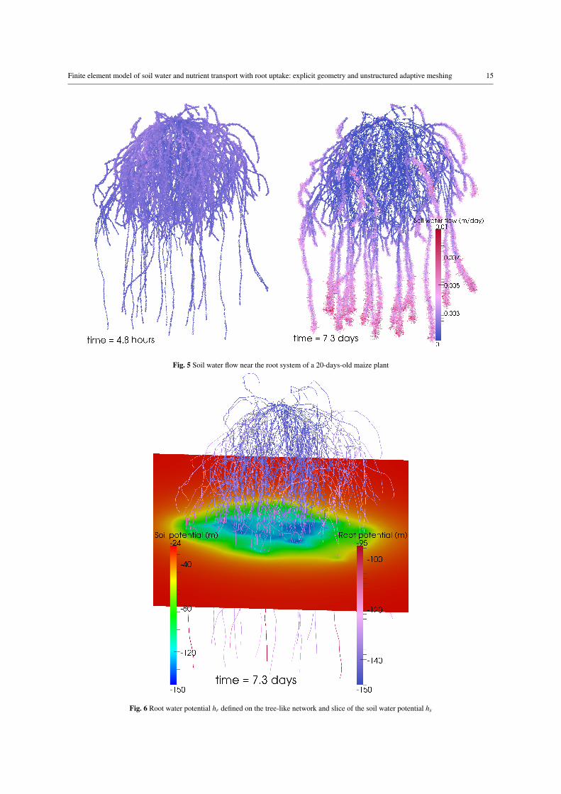
The first numerical simulation involves the 20-days-old maize root system generated by the Matlab code Root-Box depicted in Fig. 1. The soil domain is of dimensions 0.4 m × 0.4 m × 0.4 m. No-flux boundary conditionsare imposed on the boundaries of the soil domain. A constant transpiration rate equal to 1.44×10−4 m3 d−1 is im-posed at the root collar. The time step ∆ t is taken constant equal to 0.05 d. Numerical results are depicted in Figs.5 and 6. Fig. 5 shows the Darcy flux q in the vicinity of the roots. In the beginning of the simulation, root wateruptake is still relatively evenly distributed over the dense upper portion of the root system (left picture, t = 4.8h).As time passes, the uptake pattern is modified. The soil dries in the dense root zone and the root system takes upwater from wetter zones (mostly in the deeper part of the soil profile) in order to maintain a constant transpirationrate (right picture, t = 7.3d).Fig. 6 shows high gradients developing in the vicinity of the roots as the soil dries.

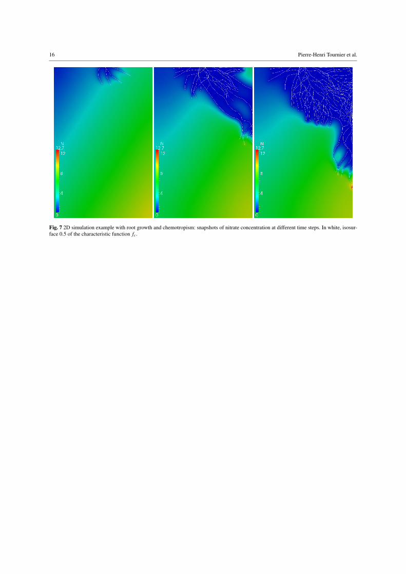
The second example illustrates how we are able to integrate root growth and chemotropism in 2D by couplingthe model with the implementation of growth and tropisms in RootBox.RootBox can simulate root tip response to mechanical soil heterogeneities as well as various types of tropisms likegravitropism, hydrotropism or chemotropism. The specific growth behaviour can be chosen for every root type.In RootBox, the implementation of tropisms consists in computing the new growth direction by random minimiza-tion of an objective function: for each active root tip, several rotations are randomly computed and the one thatleads to minimizing the objective function is chosen. Different types of tropisms are realized by choosing appro-priate objective functions depending on soil properties (water content, nutrient concentration). In this example, acombination of gravitropism and chemotropism is achieved by defining the objective function as −λc+ z whereλ > 0 represents the relative strength of chemotropism.At each time step, an iteration of the following coupling algorithm is performed:

1. RootBox finds the best growth direction for each active root tip through multiple evaluations of the objectivefunction depending on the spatial concentration c. RootBox is interfaced with the FreeFem++ finite elementcode so that the values of the concentration can be determined by interpolation on the mesh. Then, a newtree-like network with new root segments is obtained.

2. A mesh adapted to the new characteristic function fc is obtained from the previous mesh by the mesh adapta-tion procedure described in section 5.

3. Finite element functions (namely the current soil water potential and N concentration) are interpolated fromthe previous mesh to the new mesh.

4. Solve (2.12) and (3.11) and obtain the new soil water potential and N concentration distributions.

Fig. 7 depicts some results of such a simulation with the initial nitrate concentration set to a linear profile varyingfrom 0 mol m−3 at the top left corner of the domain to 10 mol m−3 at the bottom right corner. Notice the accu-mulation of nitrate around some of the roots in the bottom right: as the soil dries out, radial soil-root water flowincreases in the bottom right where the soil is wetter, resulting in the mass flow of nitrate bringing more than theroot can take up.


8 Conclusion

In this paper we presented a model of soil water and nutrient transport with plant root uptake. A characteristicfunction of the geometry of the root system was used to construct accurate sink terms corresponding to waterand nutrient uptake by roots. An emphasis was put on the spatial discretization with an adaptive mesh refinementprocedure producing meshes that are able to resolve the complex geometry of the root system together with small-scale phenomena occuring in the rhizosphere. A parallel finite element method was then presented using a two-level Schwarz domain decomposition method to solve the potentially large systems arising from the discretization.Numerical experiments were conducted in two and three spatial dimensions to illustrate the capabilities of themodel.Future work will consist in using the diffuse domain approach to approximate the actual surface of the roots inthe volume mesh without relying on a surface mesh. The level set representing the root surface splits the domainΩ into two subdomains Ωs and Ωr. Following a monolithic approach, different problems are defined on the samemesh in the soil domain Ωs and in the root system Ωr using a phase field variable. This approach allows us tomake use of the same adaptive volume remeshing procedure that was described in this paper.

Acknowledgements We thank Pierre Jolivet for his valuable insights on FreeFem++ and domain decomposition methods.

References

1. Barber, S.A.: Soil nutrient bioavailability: a mechanistic approach. Wiley-Interscience, New York (1984)2. Barraclough, P.B., Tinker, P.B.: The determination of ionic diffusion coefficients in field soils. I. diffusion coefficients in sieved soils in

relation to water content and bulk density. Journal of Soil Science 32(2), 225–236 (1981)3. Berninger, H.: Domain decomposition methods for elliptic problems with jumping nonlinearities and application to the richards equation.

Ph.D. thesis, Freie Universitat Berlin (2007)4. Celia, M.A., Bouloutas, E.T., Zarba, R.L.: A general mass-conservative numerical solution for the unsaturated flow equation. Water

Resources Research 26(7), 1483–1496 (1990)5. Dobrzynski, C.: MMG3D: User Guide. Rapport Technique RT-0422, INRIA (2012)6. Doussan, C., Pages, L., Vercambre, G.: Modelling of the hydraulic architecture of root systems: An integrated approach to water absorption

- model description. Annals of Botany 81, 213–223 (1998)7. Doussan, C., Pierret, A., Garrigues, E., Pages, L.: Water uptake by plant roots: II - modelling of water transfer in the soil root-system with

explicit account of flow within the root system - comparison with experiments. Plant and Soil 283(1-2), 99–117 (2006)8. Fiscus, E.L.: The interaction between osmotic- and pressure-induced water flow in plant roots. Plant Physiology 55(5), 917–922 (1975)9. Hecht, F.: New development in freefem++. Journal of Numerical Mathematics 20, 251–266 (2013)

10. Hopmans, J.W., Bristow, K.L.: Current capabilities and future needs of root water and nutrient uptake modeling. In: D.L. Sparks (ed.)Advances in Agronomy, Advances in Agronomy, vol. 77, pp. 103 – 183. Academic Press (2002)

11. Javaux, M., Schroder, T., Vanderborght, J., Vereecken, H.: Use of a three-dimensional detailed modeling approach for predicting rootwater uptake. Vadose Zone Journal 7, 1079–1088 (2008)

12. Ji, S.H., Park, Y.J., Sudicky, E.A., Sykes, J.F.: A generalized transformation approach for simulating steady-state variably-saturated sub-surface flow. Advances in Water Resources 31(2), 313–323 (2008)

13. Jolivet, P., Dolean, V., Hecht, F., Nataf, F., Prud’homme, C., Spillane, N.: High performance domain decomposition methods on massivelyparallel architectures with freefem++. Journal of Numerical Mathematics 20, 287–302 (2013)

14. Karypis, G., Kumar, V.: A fast and high quality multilevel scheme for partitioning irregular graphs. SIAM Journal on Scientific Computing20, 359–392 (1998)

15. Kochian, L.V., Lucas, W.J.: Potassium transport in corn roots: I. resolution of kinetics into a saturable and linear component. PlantPhysiology 70(6), 1723–1731 (1982)

16. Kool, J.B., Parker, J.C.: Development and evaluation of closed-form expressions for hysteretic soil hydraulic properties. Water ResourcesResearch 23(1), 105–114 (1987)

17. Landsberg, J., Fowkes, N.: Water movement through plant roots. Annals of Botany 42(1), 493–508 (1978)18. Leitner, D., Klepsch, S., Bodner, G., Schnepf, A.: A dynamic root system growth model based on l-systems. Plant and Soil 332(1-2),

177–192 (2010)19. McGechan, M., Lewis, D.: Sorption of phosphorus by soil, part 1: Principles, equations and models. Biosystems Engineering 82, 1–24

(2002)20. Pop, I.S.: Error estimates for a time discretization method for the richards’ equation. Computational Geosciences 6(2), 141–160 (2002)21. Saaltink, M.W., Carrera, J., Olivella, S.: Mass balance errors when solving the convective form of the transport equation in transient flow

problems. Water Resources Research 40(5) (2004)22. Somma, F., Hopmans, J., Clausnitzer, V.: Transient three-dimensional modeling of soil water and solute transport with simultaneous root

growth, root water and nutrient uptake. Plant and Soil 202(2), 281–293 (1998)23. Stevens, D., Power, H.: A scalable and implicit meshless RBF method for the 3D unsteady nonlinear richards equation with single and

multi-zone domains. International Journal for Numerical Methods in Engineering 85(2), 135–163 (2011)24. Tuzet, A., Perrier, A., Leuning, R.: A coupled model of stomatal conductance, photosynthesis and transpiration. Plant, Cell & Environment

26(7), 1097–1116 (2003)


25. Varado, N., Braud, I., Ross, P., Haverkamp, R.: Assessment of an efficient numerical solution of the 1d richards’ equation on bare soil.Journal of Hydrology 323(1-4), 244–257 (2006)

26. Vohralık, M., Wheeler, M.: A posteriori error estimates, stopping criteria, and adaptivity for two-phase flows. Computational Geosciences17(5), 789–812 (2013)

27. Simunek, J., Hopmans, J.W.: Modeling compensated root water and nutrient uptake. Ecological Modelling 220(4), 505–521 (2009)


Fig. 5 Soil water flow near the root system of a 20-days-old maize plant

Fig. 6 Root water potential hr defined on the tree-like network and slice of the soil water potential hs


Fig. 7 2D simulation example with root growth and chemotropism: snapshots of nitrate concentration at different time steps. In white, isosur-face 0.5 of the characteristic function fc.

finite element model of soil water and nutrient transport ...comte/pdf/article2.pdf · finite...

Documents