financial projections forecast—budget—analyze. three methods of analyzing financial statements...

Financial ProjectionsForecast—Budget—Analyze

Three Methods of Analyzing Financial Statements

• Vertical analysis

• Horizontal analysis

• Ratio analysis

Vertical Analysis

• Vertical analysis is the process of using a single variable on a financial statement as a constant and determining how all of the other variables relate as a percentage of the single variable.

Vertical Analysis of an Income Statement

• The vertical analysis of the income statement is used to determine, specifically, how much of a company’s net sales consumed by each individual entry on the income statement.

• Constant is net sales.

100$in SalesNet

$in ItemStatement Income SalesNet of Percentage

The formula is:

Horizontal Analysis

• Horizontal analysis is a determination of the percentage increase or decrease in an account from a base time period to successive time periods.

Percentage Change New time period amount - Old time period amount

Old time period amount100

The basic formula is:

Gross sales 300,580$ 315,487$ 101.73 4.96Less returns 5,124 9,253 1.73 80.58Net sales 295,456 306,234 100.00 3.65Cost of goods sold 101,250 120,002 34.27 18.52Gross profit 194,206 186,232 65.73 (4.11)Operating expenses Administration 74,983 76,450 25.38 1.96 Advertising 35,214 37,250 11.92 5.78 Overhead 27,120 28,300 9.18 4.35Operating income 56,889 44,232 19.25 (22.25)Interest 7,000 6,250 2.37 (10.71)Earnings before taxes 49,889 37,982 16.89 (23.87)Taxes 7,483 5,697 2.53 (23.87)Net profit 42,406$ 32,285$ 14.35 (23.87)

Horizontal Analysis 2005-

2006 (%)Account Year 2005 Year 2006

Vertical Analysis 2005 (%)

Table 4-1 Sample Income Statement Data

Markadel Retail StoreIncome Statement Data

From January 1 through December 31, 2007 and 2008

Vertical Analysis of a Balance Sheet

• Vertical analysis of the balance sheet is always carried out by using total assets as a constant, or 100 percent, and dividing every figure on the balance sheet by total assets.

100$in Assets Total

$in ItemSheet Balance Assets Total of Percentage

Table 4-2 Sample Balance Sheet Data

Current assets Cash 10,210$ 8,175$ 4.77 (19.93) Notes receivable 5,280 8,102 2.47 53.45 Accounts receivable 15,320 18,025 7.16 17.66 Inventory 35,020 50,515 16.37 44.25 Total current assets 65,830 84,817 30.77 28.84Fixed assets Land 25,000 25,000 11.69 0.00 Buildings 135,000 135,000 63.10 0.00 Accumulated depreciation (47,000) (50,000) 21.97 6.38 Equipment 58,250 58,250 27.23 0.00 Accumulated depreciation (23,150) (28,150) 10.82 21.60 Total fixed assets 148,100 140,100 69.23 (5.40)Total assets 213,930$ 224,917$ 100.00 5.14

Current liabilities Accounts payable 34,250 40,003 16.01 16.80 Notes payable 25,000 33,035 11.69 32.14 Total current liabilities 59,250 73,038 27.70 23.27Long-term debt Mortgage payable 65,000 63,000 30.38 (3.08) Bank loan payable 10,000 15,000 4.67 50.00 Total long-term debt 75,000 78,000 35.06 4.00Total liabilities 134,250 151,038 62.75 12.51Owner’s equity 79,680 73,879 37.25 (7.28)Total liabilities and owner’s equity 213,930$ 224,917$ 100.00 5.14

Markadel Retail StoreBalance Sheet Data

As of December 31, 2007 and 2008

Category

Horizontal Analysis

2007-2008 (%)

Vertical Analysis 2007 (%)Year 2007 Year 2008

Ratio Analysis

• Ratio analysis is used to determine the health of a business, especially as that business compares to other firms in the same industry or similar industries.

• A ratio is nothing more than a relationship between two variables, expressed as a fraction.

Types of Business Ratios

• Liquidity ratios determine how much of a firm’s current assets are available to meet short-term creditors’ claims.

• Activity (Efficiency) ratios indicate how efficiently a business is using its assets.

• Leverage (debt) ratios indicate what percentage of the business assets is financed with creditors’ dollars.

Types of Business Ratios (continued)

• Profitability ratios are used by potential investors and creditors to determine how much of an investment will be returned from either earnings on revenues or appreciation of assets.

• Market ratios are used to compare firms within the same industry. They are primarily used by investors to determine if they should invest capital in the company in exchange for ownership.

Liquidity Ratios

• Current Ratio: The current ratio is calculated by dividing total current assets by total current liabilities.

sliabilitie Current

Assets Current Ratio Current

The current ratio is given by the following:

Liquidity Ratios (continued)• Quick, or Acid Test, Ratio: This ratio does not

count the sale of the company’s inventory or prepaids. It measures the ability of the firm to meet its short-term obligations without liquidating its inventory.

sliabilitieCurrent

prepaids-inventory - assetsCurrent RatioQuick

The acid test ratio is given by the following:

Activity Ratios• Inventory turnover ratio (or, simply,

inventory turnover) indicates how efficiently a firm is moving its inventory. It basically states how many times per year the firm moves it average inventory.

Costat Inventory Average

COGS turnover Inventory

2

inventory Ending inventory Beginning inventory Average

Inventory turnover is given as follows:

Activity Ratios (continued)• Accounts receivable turnover ratio allows us

to determine how fast our company is turning its credit sales into cash.

Credit salesAccounts receivable turnover

Average accounts receivable

Accounts receivable turnover is given by the following:

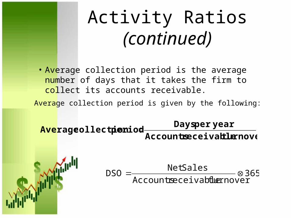
Activity Ratios (continued)

• Average collection period is the average number of days that it takes the firm to collect its accounts receivable.

turnover receivable Accounts

yearper Days period collection Average

Average collection period is given by the following:

365 turnoverreceivable Accounts

SalesNet DSO


• Fixed asset turnover ratio indicates how efficiently fixed assets are being used to generate revenue for a firm.

Net salesFixed asset turnover

Average fixed assets

Fixed asset turnover is given by the following:


• Total asset turnover ratio indicates how efficiently our firm uses its total assets to generate revenue for the firm.

Net salesTotal asset turnover

Average total assets

Total asset turnover is given by the following:

Leverage Ratios• Debt-to-equity ratio indicates what percentage of the owner’s equity is

debt.

Debt-to-equity is given by the following:

equity sOwner'

sliabilitie Total ratioequity -to-Debt

Leverage Ratios (continued)

• Debt-to-total-assets ratio indicates what percentage of a business’s assets is owned by creditors.

assets Total

sliabilitie Total ratioasset -total-to-Debt

Debt-to-total-assets is given by the following:

Leverage Ratios (continued)

• Times-interest-earned ratio shows the relationship between operating income and the amount of interest in dollars the company has to pay to its creditors on an annual basis.

Interest

income Operating ratio earned-interest-Times

Times-interest-earned is given by the following:

Profitability Ratios

• Gross profit margin ratio is used to determine how much gross profit is generated by each dollar in net sales.

sales Net

profit Gross ratio margin profit Gross

Gross profit margin is given by the following:

Profitability Ratios (continued)

• Operating profit margin ratio is used to determine how much each dollar of sales generates in operating income.

sales Net

income Operating ratio margin profit Operating

Operating profit margin is given by the following:


• Net profit margin ratio tells us how much a firm earned on each dollar in sales after paying all obligations including interest and taxes.

sales Net

profit Net ratio margin profit Net

Net profit margin is given by the following:


• Operating return on assets ratio is also referred to as operating return on investment and allows us to determine how much we are actually earning on each dollar in assets prior to paying interest and taxes.

Operating incomeOperating return on assets


Operating return on assets is given by the following:

Profitability Ratios (continued)• Net return on assets (ROA) ratio is also

referred to as net return on investment and tells us how much a firm earns on each dollar in assets after paying both interest and taxes.

Net profitNet return on assets ratio


Net return on assets is given by the following:

This Ratio is the same as Return on Investment (ROI)

Earning Power

Profitability Ratios (continued)• Return on equity (ROE) ratio tells the stockholder, or

individual owner, what each dollar of his or her investment is generating in net income.

Net ProfitReturn on equity ratio

Average owner's equity

Return on equity (ROE) is given by the following:

Market Ratios• Earnings per share ratio is nothing more than the net

profit or net income of the firm, less preferred dividends (if the company has preferred stock), divided by the number of shares of common stock outstanding (issued).

Net income - Preferred dividendsEarnings per share ratio

Weighted average number of common shares outstanding

Earnings per share is given by the following:

Market Ratios (continued)• Price earnings ratio is a magnification of earnings

per share in terms of market price of stock.

share per Earnings

stock of price Market ratio earnings Price

Price earnings ratio is given by the following:

Price Earnings to Growth ratio(PEG ratio)

• The price earnings to growth ratio (PEG ratio) compares the company’s price earnings ratio to its expected earnings per share (EPS) growth rate over the next several years.

Price earnings ratioPEG ratio=

Annual expected growth rate in %

The PEG ratio is given by the following formula:

Market Ratios (continued)

• Operating cash flow per-share ratio compares the operating cash flow on the statement of cash flows to the number of shares of common stock outstanding.

Operating cash flowOperating cash flow per share

Average common shares of stock outstanding

Operating cash flow is given by the following:

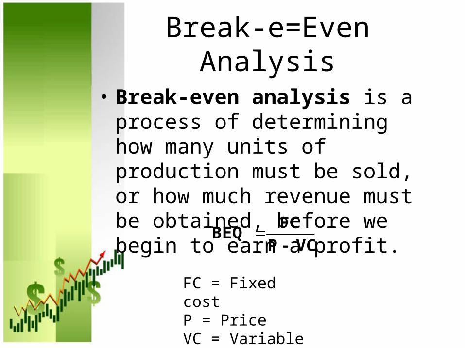
Break-e=Even Analysis

• Break-even analysis is a process of determining how many units of production must be sold, or how much revenue must be obtained, before we begin to earn a profit.

VC- P

FC BEQ

FC = Fixed costP = PriceVC = Variable Cost

Break-Even Graph

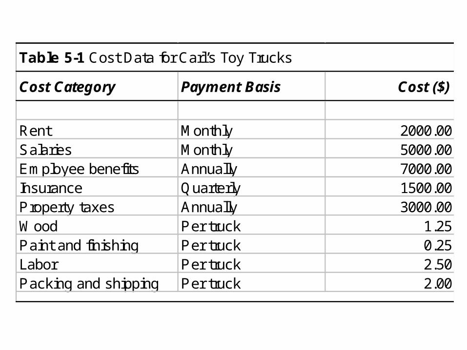
Cost Category Payment Basis Cost ($)

Rent Monthly 2000.00Salaries Monthly 5000.00Employee benefits Annually 7000.00Insurance Quarterly 1500.00Property taxes Annually 3000.00Wood Per truck 1.25Paint and finishing Per truck 0.25Labor Per truck 2.50Packing and shipping Per truck 2.00

Table 5-1 Cost Data for Carl’s Toy Trucks

Break-Even Analysis (continued)

• Break-even dollars:

Where VC is variable cost expressed as a percentage of sales (revenue).– For retail firm: VC percentage =(Cost of

Goods Sold)/(Net Sales)– For manufacturing firm: VC percentage

= (Variable cost of a unit)/(Selling price)

P

VCFC

BE

1

$

Break-Even Analysis (continued)

• Contribution margin is the amount of profit that will be made by a company on each unit that is sold above and beyond the break-even quantity.

• Contribution margin is also the amount the company will lose for each unit of production by which it falls short of the break-even point.

Profit and Break-Even• Desired profit with break-even analysis in

quantity to produce.

– VC is variable cost per unit

• Desired profit with break-even analysis in dollars.

– VC is a percentage of sales dollar (e.g., cost of goods sold as a percent).

VC - P

profit Desired FC quantity Total

dollar) sales theof percentage a (as VC-1

profit Desired $

FCBE

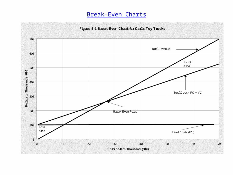
Break-Even Charts

Figure 5-1 Break-Even Chart for Carl's Toy Trucks

0

100

200

300

400

500

600

700

0 10 20 30 40 50 60 70

Units Sold in Thousand (000)

Do

llars

in T

ho

usa

nd

s (0

00)

Total Revenue

Total Cost = FC + VC

Break-Even Point

Fixed Costs (FC)

LossArea

Profit Area

Leverage

• Leverage uses those items that have a fixed cost to magnify the return to a company. Fixed costs can be related to company operations or related to the cost of financing.– Interest expenses paid on the amount

of debt incurred is the fixed cost of financing.

– A firm is heavily financially leveraged if the fixed costs of financing are high.

Leverage (continued)

• Degree of operating leverage (DOL) is the percentage change in operating income divided by the percentage change in sales.

salesin change Percentage

income operatingin change Percentage DOL


• Degree of financial leverage (DFL) is the percentage change in earnings per share divided by the percentage change in operating income.

income operatingin change Percentage

shareper earningsin change Percentage DFL


• Degree of combined leverage (DCL) is the percentage change in earnings per share divided by the percentage change in sales.

sales change Percentage

shareper earningsin change Percentage DCL

income operatingin change Percentage

shareper earningsin change Percentage

salesin change Percentage

income operatingin change Percentage DCL x

Leverage Ratios Applied

• If the DOL is 3, then for every percentage of increase in net sales an equal increase in operating income will be realized.

• However for percentage decrease an equal decrease in operating income will be realized.

Types of Forecasting Models

• Judgmental models, which use qualitative methods

• Time series models, which use quantitative methods

• Causal models, which use cause-and-effect methods

Judgmental Models

• Judgmental models are qualitative and essentially use estimates based on expert opinion. – Survey of Sales Forces: most

appropriate for manufacturing and wholesale firms.

– Surveys of Customers: applicable to all firms. Customers express preference for new or modified products.

Judgmental Models (continued)

– Historical Analogy most appropriate for firms that have several outlets. Introduction of new product which has characteristics similar to previous products.

– Market Research can include surveys, tests, and observations. Results are statistically extrapolated to develop forecasts of demand for products.

Judgmental Models (continued)

• Delphi Method uses a panel of experts to obtain a consensus of opinion. Used primarily for unique new products or processes for which no previous data exist.

Time Series Models

• Time series forecasting models normally use historical records that are readily available within the firm or industry to predict future sales. – For this reason they are often referred

to as internal or intrinsic models. – Assumption in time series forecasting is

that past sales are a fairly accurate predictor of future sales.

Time Series Models (continued)

• Moving average model• Weighted moving average model• Exponential smoothing model• Linear regression model

Table 6-1 Moving Average Model

Formula for Moving Average:

Year0

Year 1 Jan 1 245Feb 2 244Mar 3 250Apr 4 260 246.33 13.67 13.67May 5 265 251.33 13.67 13.67 249.75 15.25Jun 6 260 258.33 1.67 1.67 254.75 5.25Jul 7 255 261.67 (6.67) 6.67 258.75 3.75Aug 8 245 260.00 (15.00) 15.00 260.00 15.00Sep 9 240 253.33 (13.33) 13.33 256.25 16.25Oct 10 255 246.67 8.33 8.33 250.00 5.00Nov 11 265 246.67 18.33 18.33 248.75 16.25Dec 12 270 253.33 16.67 16.67 251.25 18.75

Year 2 Jan 13 250 263.33 (13.33) 13.33 257.50 7.50Feb 14 250 261.67 (11.67) 11.67 260.00 10.00Mar 15 258 256.67 1.33 1.33 258.75 0.75Apr 16 267 252.67 14.33 14.33 257.00 10.00May 17 273 258.33 14.67 14.67 256.25 16.75Jun 18 278 266.00 12.00 12.00 262.00 16.00Jul 19 260 272.67 (12.67) 12.67 269.00 9.00Aug 20 256 270.33 (14.33) 14.33 269.50 13.50Sep 21 255 264.67 (9.67) 9.67 266.75 11.75Oct 22 270 257.00 13.00 13.00 262.25 7.75Nov 23 275 260.33 14.67 14.67 260.25 14.75Dec 24 283 266.67 16.33 16.33 264.00 19.00

Year 3 Jan 25 276.00 270.75SD|A-F|= 62.00 255.33 232.25n= 21 21 20MAD= 2.95 12.16 11.61

Absolute DeviationD|A-F|

4 Month Moving

Average

Moving Average = Forecast

Time Period

Actual Sales

3 Month Moving

AverageMonth

Actual Numerical Deviation = Actual -Forecast

Absolute DeviationD|A-F|

n

AAAF ttnt

t

1])1[(

1

...

Year MonthTime

PeriodActual Sales

W1=0.1, W2=0.3, W3=0.6 D |A-F|

W1=0.25, W2=0.35, W3=0.40 D |A-F|

W1=4 W2=5 W3=8 D|A-F|

0Year 1 Jan 1 245

Feb 2 244Mar 3 250Apr 4 260 247.70 12.30 246.65 13.35 247.06 12.94May 5 265 255.40 9.60 252.50 12.50 253.29 11.71Jun 6 260 262.00 2.00 259.50 0.50 260.00 0.00Jul 7 255 261.50 6.50 261.75 6.75 261.47 6.47Aug 8 245 257.50 12.50 259.25 14.25 258.82 13.82Sep 9 240 249.50 9.50 252.25 12.25 251.47 11.47Oct 10 255 243.00 12.00 245.50 9.50 245.00 10.00Nov 11 265 249.50 15.50 247.25 17.75 248.24 16.76Dec 12 270 259.50 10.50 255.25 14.75 256.18 13.82

Year 2 Jan 13 250 267.00 17.00 264.50 14.50 265.00 15.00Feb 14 250 257.50 7.50 260.75 10.75 259.41 9.41Mar 15 258 252.00 6.00 255.00 3.00 254.71 3.29Apr 16 267 254.80 12.20 253.20 13.80 253.76 13.24May 17 273 262.60 10.40 259.60 13.40 260.35 12.65Jun 18 278 269.70 8.30 267.15 10.85 267.71 10.29Jul 19 260 275.40 15.40 273.50 13.50 273.94 13.94Aug 20 256 266.70 10.70 269.55 13.55 268.35 12.35Sep 21 255 259.40 4.40 262.90 7.90 262.35 7.35Oct 22 270 255.80 14.20 256.60 13.40 256.47 13.53Nov 23 275 264.10 10.90 261.25 13.75 262.29 12.71Dec 24 283 271.50 11.50 268.25 14.75 268.82 14.18

Year 3 Jan 25 279.30 276.95 277.59SD|A-F| = 218.90 244.75 234.94n = 21.00 21.00 21.00MAD = 10.42 11.65 11.19

Table 6-2 Weighted Moving Average Model

Formula for weighted moving average:

W

AWAWAWF ttttt S

3122

financial projections forecast—budget—analyze. three methods of analyzing financial statements...

Documents