financial dependence analysis: applications of … dependence analysis: applications of vine copulas...

Financial Dependence Analysis: Applications of Vine Copulas

David.E. Allena,∗, Mohammad.A. Ashrafb, Michael. McAleerc, Robert.J. Powella, and Abhay.K. Singha

aSchool of Accounting, Finance and Economics, Edith Cowan University, AustraliabIndian Institute of Technology, Kharagpur, India

cEconometric Institute, Erasmus School of Economics, Erasmus University Rotterdam, Tinbergen Institute, TheNetherlands, Department of Quantitative Economics, Complutense University of Madrid, Spain, and Institute of

Economic Research, Kyoto University, Japan

Abstract

This paper features the application of a novel and recently developed method of statistical and mathe-matical analysis to the assessment of financial risk: namely Regular Vine copulas. Dependence modellingusing copulas is a popular tool in financial applications, but is usually applied to pairs of securities. Vinecopulas offer greater flexibility and permit the modelling of complex dependency patterns using the richvariety of bivariate copulas which can be arranged and analysed in a tree structure to facilitate the anal-ysis of multiple dependencies. We apply Regular Vine copula analysis to a sample of stocks comprisingthe Dow Jones Index to assess their interdependencies and to assess how their correlations change indifferent economic circumstances using three different sample periods: pre-GFC (Jan 2005- July 2007),GFC (July 2007-Sep 2009), and post-GFC periods (Sep 2009 - Dec 2011). The empirical results suggestthat the dependencies change in a complex manner, and there is evidence of greater reliance on the Stu-dent t copula in the copula choice within the tree structures for the GFC period, which is consistent withthe existence of larger tails in the distributions of returns for this period. One of the attractions of thisapproach to risk modelling is the flexibility in the choice of distributions used to model co-dependencies.The practical application of Regular Vine metrics is demonstrated via an example of the calculation ofthe VaR of a portfolio of stocks.

Keywords: Regular Vine Copulas, Tree structures, Co-dependence modelling.

JEL Codes: G11, C02.

1. Introduction

In the last decade copula modelling has become a frequently used tool in financial economics. Accountsof copula theory are available in Joe (1997) and Nelsen (2006). Hierarchical, copula-based structures haverecently been used in some new developments in multivariate modelling; notable among these structuresis the pair-copula construction (PCC). Joe (1996) originally proposed the PCC and further explorationof its properties has been undertaken by Bedford and Cooke (2001, 2002) and Kurowicka and Cooke(2006). Aas et al. (2009) provided key inferential insights which have stimulated the use of the PCCin various applications, (see, for example, Schirmacher and Schirmacher (2008), Chollete et al. (2009),Heinen and Valdesogo (2009), Berg and Aas (2009), Min and Czado (2010), and Smith et al. (2010).

There have also been some recent applications of copulas in the context of time series models (seethe survey by Patton (2009), and the recently developed COPAR model of Breckmann and Czado(2012), which provides a vector autoregressive VAR model for analysing the non-linear and asymmetricco-dependencies between two series). Nevertheless, in this paper we focus on static modelling of de-pendencies based on R Vines in the context of modelling the co-dependencies of Dow Jones IndustrialAverage (DJIA) Index constituents for three different sample periods which include the GFC. To furthershow the capabilities of this flexible modelling technique, we also use R-Vine Copulas to quantify Valueat Risk for a portfolio of ten sample stocks from DJIA as an empirical example. The main aim of thepaper is to demonstrate the useful application of the R Vine measure of co-dependency at at time ofextreme financial stress amd its finesse in teasing out changes in co-dependency.

∗Corresponding authorEmail address: [email protected] (David.E. Allen)

Preprint submitted to Elsevier May 26, 2013

2

The paper is divided into five sections: the next section provides a review of the background theoryand models applied, section 3 introduces the sample, section 4 presents the results and a brief conclusionfollows in section 5.

2. Background and models

Sklar (1959) provides the basic theorem describing the role of copulas for describing dependence instatistics, providing the link between multivariate distribution functions and their univariate margins.We can speak generally of the copula of continuous random variables X = (X1, ....Xd) ∼ F . The problemin practical applications is the identification of the appropriate copula.

Standard multivariate copulas, such as the multivariate Gaussian or Student-t, as well as exchangeableArchimedean copulas, lack the exibility of accurately modelling the dependence among larger numbersof variables. Generalizations of these offer some improvement, but typically become rather intricate intheir structure, and hence exhibit other limitations such as parameter restrictions. Vine copulas do notsuffer from any of these problems.

Initially proposed by Joe (1996) and developed in greater detail in Bedford and Cooke (2001, 2002) andin Kurowicka and Cooke (2006), vines are a flexible graphical model for describing multivariate copulasbuilt up using a cascade of bivariate copulas, so-called pair-copulas. Their statistical breakthrough wasdue to Aas, Czado, Frigessi, and Bakken (2009) who described statistical inference techniques for the twoclasses of canonical C-vines and D-vines. These belong to a general class of Regular Vines, or R-vineswhich can be depicted in a graphical theoretic model to determine which pairs are included in a pair-copula decomposition. Therefore a vine is a graphical tool for labelling constraints in high-dimensionaldistributions.

A regular vine is a special case for which all constraints are two-dimensional or conditional two-dimensional. Regular vines generalize trees, and are themselves specializations of Cantor trees. Combinedwith copulas, regular vines have proven to be a flexible tool in high-dimensional dependence modelling.Copulas are multivariate distributions with uniform univariate margins. Representing a joint distribu-tion as univariate margins plus copulas allows the separation of the problems of estimating univariatedistributions from problems of estimating dependence.

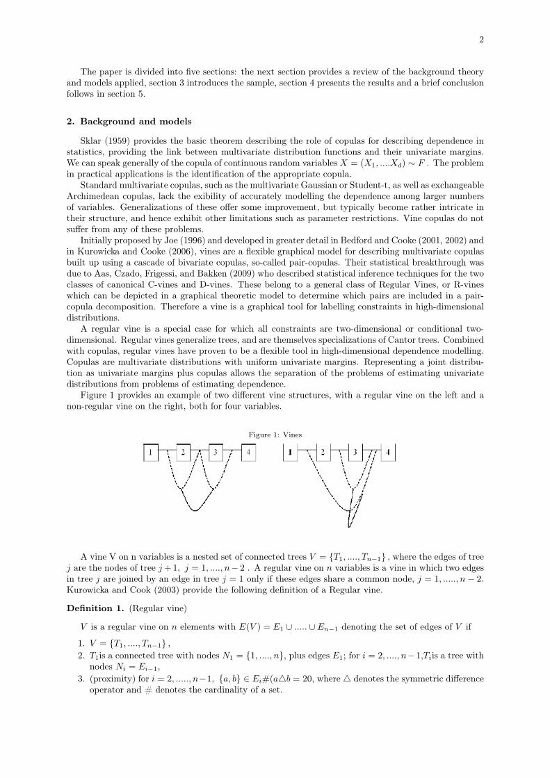
Figure 1 provides an example of two different vine structures, with a regular vine on the left and anon-regular vine on the right, both for four variables.

Figure 1: Vines

A vine V on n variables is a nested set of connected trees V = {T1, ...., Tn−1} , where the edges of treej are the nodes of tree j+ 1, j = 1, ...., n− 2 . A regular vine on n variables is a vine in which two edgesin tree j are joined by an edge in tree j = 1 only if these edges share a common node, j = 1, ....., n− 2.Kurowicka and Cook (2003) provide the following definition of a Regular vine.

Definition 1. (Regular vine)

V is a regular vine on n elements with E(V ) = E1 ∪ ..... ∪ En−1 denoting the set of edges of V if

1. V = {T1, ...., Tn−1} ,2. T1is a connected tree with nodes N1 = {1, ...., n}, plus edges E1; for i = 2, ...., n−1,Tiis a tree with

nodes Ni = Ei−1,3. (proximity) for i = 2, ....., n−1, {a, b} ∈ Ei#(a4b = 20, where4 denotes the symmetric difference

operator and # denotes the cardinality of a set.

2.1 Modelling Vines 3

An edge in a tree Tj is an unordered pair of nodes of Tj or equivalently, an unordered pair of edges ofTj−1. By definition, the order of an edge in tree Tj is j − 1, j = 1, ..., n − 1. The degree of a node isdetermined by the number of edges attached to that node. A regular vine is called a canonical vine, orC−vine, if each tree Ti has a unique node of degree n − 1 and therefore, has the maximum degree. Aregular vine is termed a D−vine if all the nodes in T1 have degrees no higher than 2.

Definition 2. (The following definition is taken from Cook et al. (2011)). For e ∈ Ei, i ≤ n − 1,the constraint set associated with e is the complete union of U∗e of e, which is the subset of {1, ...., n}reachable from e by the membership relation.

For i = 1, ...., n− 1, e ∈ Ei, if e = {j, k}, then the conditioning set associated with e is

De = U∗j ∩ U∗k

and the conditioned set associated with e is

{Ce,j , Ce,k} ={U∗j \De, U

∗k \De

}.

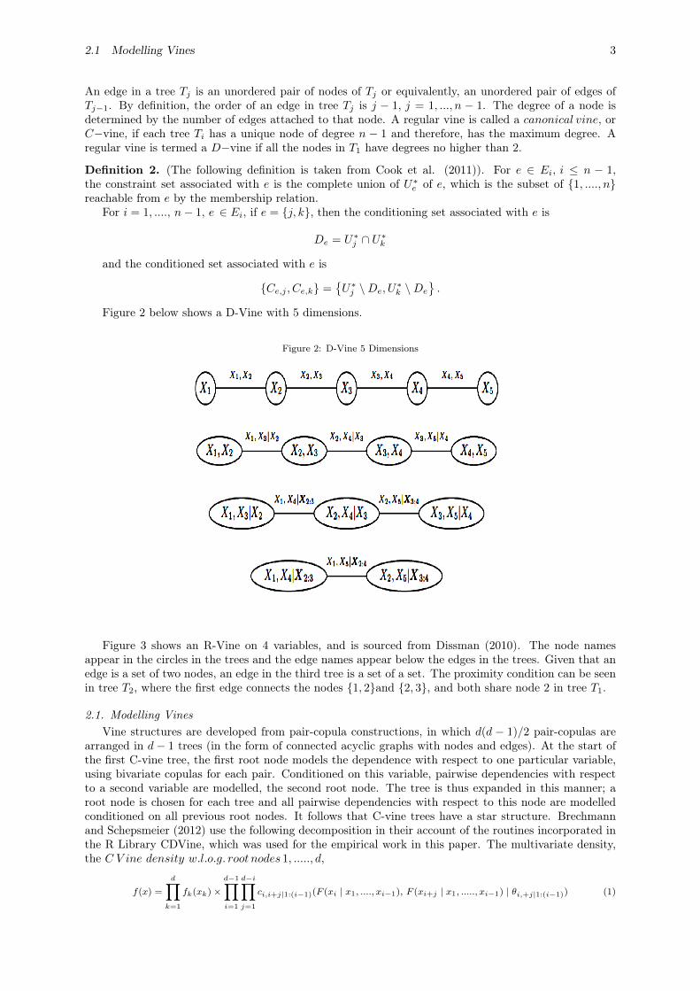
Figure 2 below shows a D-Vine with 5 dimensions.

Figure 2: D-Vine 5 Dimensions

Figure 3 shows an R-Vine on 4 variables, and is sourced from Dissman (2010). The node namesappear in the circles in the trees and the edge names appear below the edges in the trees. Given that anedge is a set of two nodes, an edge in the third tree is a set of a set. The proximity condition can be seenin tree T2, where the first edge connects the nodes {1, 2}and {2, 3}, and both share node 2 in tree T1.

2.1. Modelling VinesVine structures are developed from pair-copula constructions, in which d(d − 1)/2 pair-copulas are

arranged in d− 1 trees (in the form of connected acyclic graphs with nodes and edges). At the start ofthe first C-vine tree, the first root node models the dependence with respect to one particular variable,using bivariate copulas for each pair. Conditioned on this variable, pairwise dependencies with respectto a second variable are modelled, the second root node. The tree is thus expanded in this manner; aroot node is chosen for each tree and all pairwise dependencies with respect to this node are modelledconditioned on all previous root nodes. It follows that C-vine trees have a star structure. Brechmannand Schepsmeier (2012) use the following decomposition in their account of the routines incorporated inthe R Library CDVine, which was used for the empirical work in this paper. The multivariate density,the C V ine density w.l.o.g. root nodes 1, ....., d,

f(x) =

d∏k=1

fk(xk)×d−1∏i=1

d−i∏j=1

ci,i+j|1:(i−1)(F (xi | x1, ...., xi−1), F (xi+j | x1, ....., xi−1) | θi,+j|1:(i−1)) (1)

2.2 Regular vines 4

where fk, k = 1, ....., d, denote the marginal densities and ci,i+j|1:(i−1)bivariate copula densities withparameter(s)θi,i+j|1:(i−1) (in general, ik : immeans ik, ...., im). The outer product runs over the d − 1trees and root nodes i, while the inner product refers to the d− i pair copulas in each tree i = 1, ...., d−1.

D-Vines follow a similar process of construction by choosing a specific order for the variables. Thefirst tree models the dependence of the first and second variables, of the second and third, and so on,...using pair copulas. If we assume the order is 1, ..., d, then first the pairs (1,2), (2,3), (3,4) are modelled.In the second tree, the co-dependence analysis can proceed by modelling the conditional dependence ofthe first and the third variables, given the second variable; the pair (2, 4 | 3), and so forth. This processcan then be continued in the next tree, in which variables can be conditioned on those lying betweenentries a and b in the first tree, for example, the pair (1, 5 | 2, 3, 4). The D-Vine tree has a path structurewhich leads to the construction of the D − vine density, which can be constructed as follows:

f(x) =

d∏k=1

fk(xk)×d−1∏i=1

d−i∏j=1

cj,j+i|(j+1):(j+i−1)(F (xj | xj+1, ....., xj+i−1), F (xj+i | xj+1, ...., xj+i−1) | θj,j+i|(j+1):(j+i−1))

(2)The outer product runs over d− 1 trees, while the pairs in each tree are determined according to the

inner product. The conditional distribution functions F (x | ν) can be obtained for an m− dimensionalvector ν. This can be done in a pair copula term in tree m− 1, by using the pair-copulas of the previoustrees 1, ...., m, and by sequentially applying the following relationship:

h(x | ν, θ) := F (x | ν) =∂Cxνj |ν−j

(F (x | ν−j), F (νj | ν−j) | θ)∂F (νj | ν−j)

(3)

where νj is an arbitrary component of ν, and ν−j denotes the (m−1)- dimensional vector ν excludingνj . The bivariate copula function is specified by Cxνj |v−j with parameters θ specified in tree m.

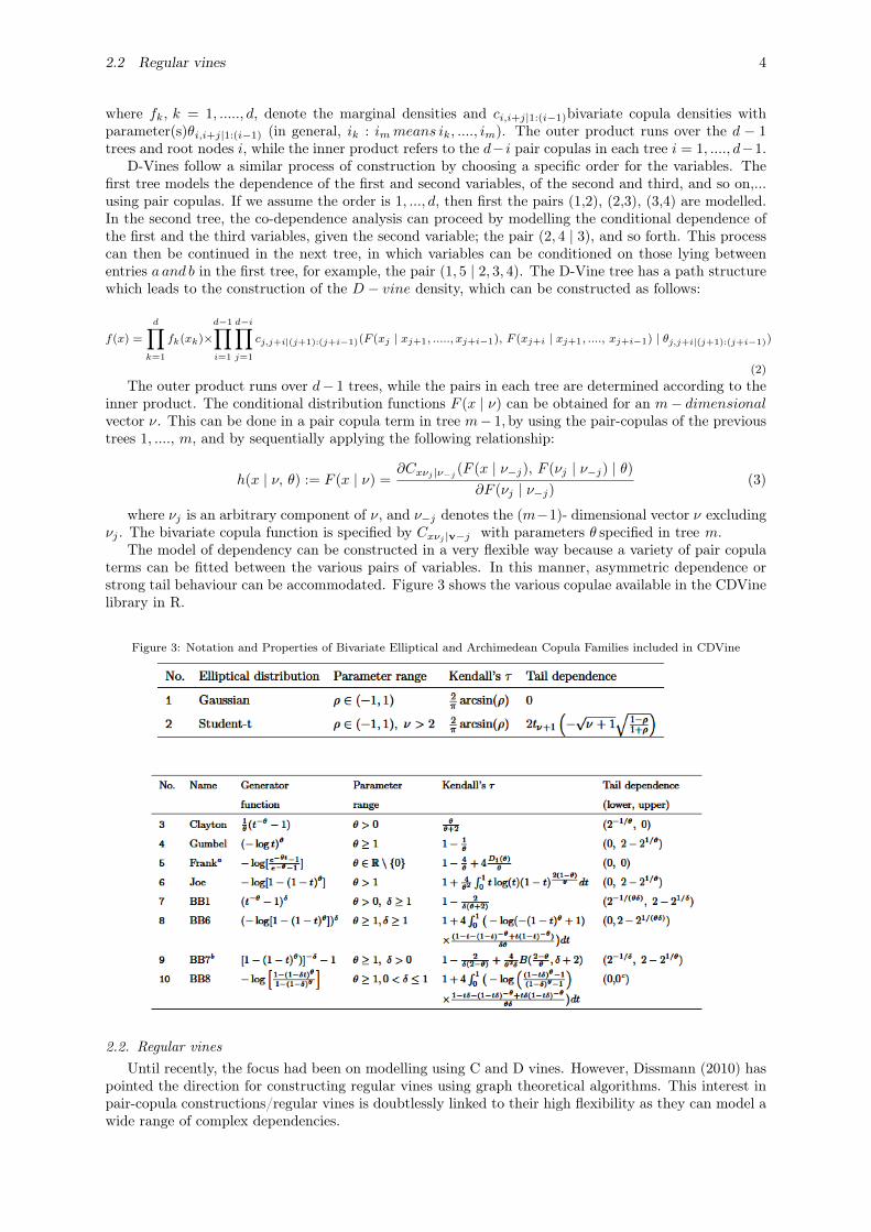
The model of dependency can be constructed in a very flexible way because a variety of pair copulaterms can be fitted between the various pairs of variables. In this manner, asymmetric dependence orstrong tail behaviour can be accommodated. Figure 3 shows the various copulae available in the CDVinelibrary in R.

Figure 3: Notation and Properties of Bivariate Elliptical and Archimedean Copula Families included in CDVine

2.2. Regular vinesUntil recently, the focus had been on modelling using C and D vines. However, Dissmann (2010) has

pointed the direction for constructing regular vines using graph theoretical algorithms. This interest inpair-copula constructions/regular vines is doubtlessly linked to their high flexibility as they can model awide range of complex dependencies.

2.2 Regular vines 5

Figure 4 shows an R-Vine on 4 variables, and is sourced from Dissman (2010). The node namesappear in the circles in the trees and the edge names appear below the edges in the trees. Given thatan edge is a set of two nodes, an edge in the third tree is a set of a set. The proximity condition can beseen in tree T2, where the first edge connects the nodes {1, 2}and {2, 3}, plus both share the node 2 intree T1.

Figure 4: Example of R-Vine on 4 Variables. (Source Dissman (2010))

The drawback is the curse of dimensionality: the computational effort required to estimate all pa-rameters grows exponentially with the dimension. Morales-Napoles et al (2009) demonstrate that there

are n!2× 2

(n− 22

)

possible R-Vines on n nodes. The key to the problem is whether the regular vinecan be either truncated or simplified. Brechmann et al, (p2, 2012) discuss such simplification methods.They explain that: “by a pairwisely truncated regular vine at level K, we mean a regular vine whereall pair-copulas with conditioning set equal to or larger than K are replaced by independence copulas”.They pairwise simplify a regular vine at level K by replacing the same pair-copulas with Gaussian cop-ulas. Gaussian copulas mean a simplification since they are easier to specify than other copulas, easy tointerpret in terms of the correlation parameter, and quicker to estimate.

They identify the most appropriate truncation/simplification level by means of statistical modelselection methods; specifically, the AIC, BIC and the likelihood-ratio based test proposed by Vuong(1989). For R-vines, in general, there are no expressions like equations (2) and (3). This means thatan efficient method for storing the indices of the pair copulas required in the joint density function, asdepicted in equation (5), is required; (5) is a more general case of (2) and (3).

f(x1, ...., xd) =

[d∏

k=1

fx(xk)

]×

[d−1∏i=1

∏e∈Ei

cj(e),k(e)|D(e)(F (xj(e) | xD(e)), F (xk(e) | xD(e)))

](4)

Kurowicka (2011) and Dissman (2010) have recently suggested a method of proceeding which involvesspecifying a lower triangular matrix M = (mi,j | i, j = 1, ...., d) ∈ {0, ..., d}d×d, with mi,i = d − i + 1.This means that the diagonal entries of M are the numbers 1, ...., d in descending order. In this matrix,each row proceeding from the bottom represents a tree, the diagonal entry represents the conditionedset and by the corresponding column entry of the row under consideration. The conditioning set is givenby the column entries below this row. The corresponding parameters and types of copula can be storedin matrices relating to M. The following example in Figure 5 is taken from Dissman (2010).

2.2 Regular vines 6

Figure 5: Matrix Mapping of vine copulas (source Dissman (2010))

The first section of Figure 5 provides a key to indicate the 5 different types of copulas used inthis example, ranging from Gaussian (1) to Frank (5). The second lower triangular matrix T1 shows theapplication of particular types of copulas in the trees, P 1

1 shows the parameters estimated, and P 21 provides

the extra parameters needed when we apply the t copula.

Figure 6: Use of Matrices to Store R-vine Information (source: Dissman (2010))

In Figure 6 the bottom row of M1corresponds to T1, the second row to T2, and so on. In order todetermine the edges in T1, we combine the numbers in the bottom row with the diagonal elements in thecorresponding columns, for example the edges are (4,3), (5,2), (1,2) and so on. In order to determinethe edges in T2, we combine the numbers in the second row from the bottom with the diagonal elementsin the corresponding columns and condition on the elements in the bottom row. This would give edges(4, 2 | 3), (5, 3 | 2), (1, 3 | 2), and so on The final entry is given by the upper entries to the left of thematrix (4, 7 | 65123).

2.3 Prior work with R-Vines 7

2.3. Prior work with R-VinesThe literature was initially mainly concerned with illustrative examples, (see, for example, Aas et al.

(2009), Berg and Aas (2009), Min and Czado (2010) and Czado et al. (2011)). Mendes et al. (2010)use a D-Vine copula model to a six-dimensional data set and consider its use for portfolio management.Dissman (2010) uses R-Vines to analyse dependencies between 16 financial indices covering differentEuropean regions and different asset classes, including five equity, nine fixed income (bonds), and twocommodity indices. He assesses the relative effectiveness of the use of copulas, based on mixed distribu-tions, t distributions and Gaussian distributions, and explores the loss of information from truncatingthe R-Vine at earlier stages of the analysis and the substitution of independence copula. He also analysesexchange rates and windspeed data sets with fewer variables.

The research in this paper extends the work of Dissman (2010) applying R-Vines to financial databy using a larger dataset; namely the Dow Jones constituent stocks and features an exploration of howtheir dependency structures change through periods of extreme stress as represented by the GFC. Thepaper also features an example of how the dependencies captured by the R-Vine analysis can be used toassess portfolio Value at Risk (VaR) in the a manner that closely parallels Breckmann and Czado (2011)who adopted a factor model approach discussed below.

There have been other studies on European stock return series: Heinen and Valdesogo (2009) con-structed a CAPM extension using their Canonical V ine Autoregressive (CAVA) model using marginalGARCH models and a canonical vine copula structure. Breckmann and Czado (2011) develop a regularvine market sector factor model for asset returns that uses GARCH models for margins, and which issimilarly developed in a CAPM framework. They explore systematic and unsystematic risk for individualstocks, and consider how vine copula models can be used for active and passive portfolio managementand VaR forecasting.

3. Sample

We use a data set of daily returns, which runs from 1 January 2005 to 31 January 2011 for the DOWJones Index and its component 30 stocks. We divide our sample into returns for the pre-GFC (Jan 2005-July 2007), GFC (July 2007-Sep 2009) and post-GFC (Sep 2009 - Dec 2011) periods. The sample forthe three periods is shown in Table 1. We analyse the behaviour of the stocks that remain constituentsof the DOW Jones index throughout the three periods. Not all Dow Jones stocks are included in eachperiod.

8

PRE GFC GFC Post GFC

V1 3M MMM 3M MMM 3M MMM

V2 ALCOA AA ALCOA AA ALCOA AA

V3 ALTRIA GRP ALTRIA AMERICAN EXPRESS AXP AMERICAN EXPRESS AXP

V4 AMERICAN EXPRESS AXP AT&T T AT&T T

V5 AMERICAN INTL GRP AIG BOEING BA BANK OF AMERICA BAC

V6 AT&T T CATERPILLAR CAT BOEING BA

V7 BOEING BA E I DU PONT DE NEMOURS DD CATERPILLAR CAT

V8 CATERPILLAR CAT EXXON MOBIL XOM CHEVRON CVX

V9 CITIBANK C GENERAL ELECTRIC GE CISCO SYSTEMS CSCO

V10 E I DU PONT DE NEMOURS DD HEWLETT-PACKARD HPQ E I DU PONT DE NEMOURS DD

V11 EXXON MOBIL XOM HOME DEPOT HD EXXON MOBIL XOM

V12 GENERAL ELECTRIC GE INTEL INTC GENERAL ELECTRIC GE

V13 HEWLETT-PACKARD HPQ INTERNATIONAL BUS.MCHS. IBM HEWLETT-PACKARD HPQ

V14 HOME DEPOT HD JOHNSON & JOHNSON JNJ HOME DEPOT HD

V15 HONEYWELL HON JP MORGAN CHASE & CO. JPM INTEL INTC

V16 INTEL INTC MCDONALDS MCD INTERNATIONAL BUS.MCHS. IBM

V17 INTERNATIONAL BUS.MCHS. IBM MERCK & CO. MRK JOHNSON & JOHNSON JNJ

V18 JOHNSON & JOHNSON JNJ MICROSOFT MSFT JP MORGAN CHASE & CO. JPM

V19 JP MORGAN CHASE & CO. JPM PFIZER PFE KRAFT FOODS KRFT

V20 MCDONALDS MCD PROCTER & GAMBLE PG MCDONALDS MCD

V21 MERCK & CO. MRK COCA COLA KO MERCK & CO. MRK

V22 MICROSOFT MSFT UNITED TECHNOLOGIES UTX MICROSOFT MSFT

V23 PFIZER PFE VERIZON COMMUNICATIONS VZ PFIZER PFE

V24 PROCTER & GAMBLE PG WAL MART STORES WMT PROCTER & GAMBLE PG

V25 COCA COLA KO WALT DISNEY DIS COCA COLA KO

V26 UNITED TECHNOLOGIES UTX DOW JONES DJIA TRAVELERS COS. TRV

V27 VERIZON COMMUNICATIONS VZ UNITED TECHNOLOGIES UTX

V28 WAL MART STORES WMT VERIZON COMMUNICATIONS VZ

V29 WALT DISNEY DIS WAL MART STORES WMT

V30 DOW JONES DJIA WALT DISNEY DIS

V31 DOW JONES DJIA

Table 1: Dow Jones Stocks used in Each Period

4. Results

The results are presented here in two parts. In the first subsection below we model the dependencestructure of DJIA stocks in three subperiods covering GFC. The second subsection gives results from anempirical exercise modelling VaR using R-Vine Copulas for a 10 asset portfolio.

4.1. Dependence Modelling Using Vine CopulaWe divide the data into three time periods covering the pre-GFC (Jan 2005- July 2007), GFC (July

2007-Sep 2009), and post-GFC periods (Sep 2009 - Dec 2011) to run the C-Vine and R-Vine dependenceanalysis for the stocks comprising Dow Jones Index. Before we can do this we require appropriatelystandardised marginal distributions for the basic company return series. These appropriate marginaltime series models for the Dow Jones data have to be found in the first step of our two step estimationapproach. The following time series models are selected in a stepwise procedure: GARCH (1,1), ARMA(1,1), AR(1), GARCH(1,1), MA(1)-GARCH(1,1). These are applied to the return data series and weselect the model with the highest p-value, so that the residuals can be taken to be i.i.d. The residuals arestandardized and the marginals are obtained from the standardized residuals using the Ranks method.These marginals are then used as inputs to the Copula selection routine. The copula are selected usingthe AIC criterion. We first discuss the results obtained from the pre-GFC period data followed by theGFC and post-GFC periods.

The following figure presents the structure of the C-Vines.

For this C Vine selection, we choose as root node the node that maximizes the sum of pairwisedependencies to this node.We commence by linking all the stocks to the Dow Jones index which is at the

4.1 Dependence Modelling Using Vine Copula 9

Figure 7: Results-C-Vine Tree-1 Pre-GFC

centre of this diagram. We use a range of Copulas from for selection purposes; the range being (1:6). Weapply AIC as the selection criterion to select from the following menu of copulae: 1 = Gaussian copula,2 = Student t copula (t-copula), 3 = Clayton copula, 4 = Gumbel copula, 5 = Frank copula, 6 = Joecopula.

We then compute transformed observations from the estimated pair copulas and these are used asinput parameters for the next trees, which are obtained similarly by constructing a graph according tothe above C-Vine construction principles (proximity conditions), and finding a maximum dependencetree. The C-Vine tree for period 2 is shown below.


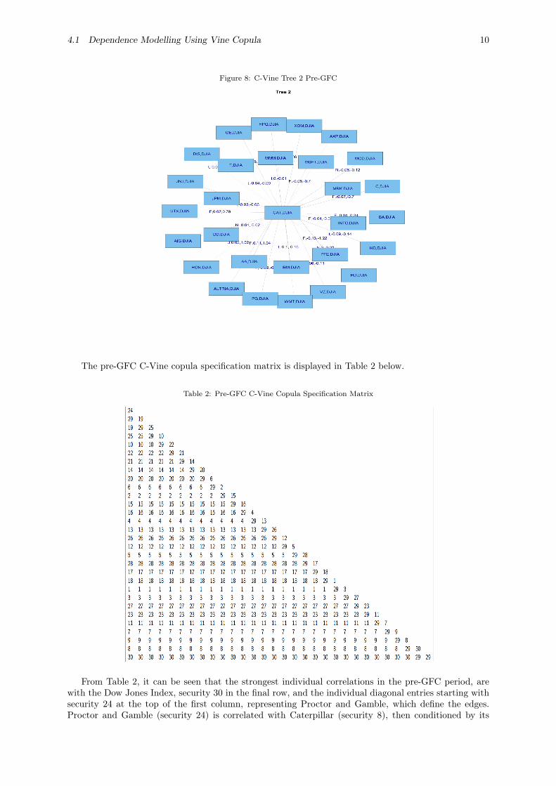
Figure 8: C-Vine Tree 2 Pre-GFC

The pre-GFC C-Vine copula specification matrix is displayed in Table 2 below.

Table 2: Pre-GFC C-Vine Copula Specification Matrix

From Table 2, it can be seen that the strongest individual correlations in the pre-GFC period, arewith the Dow Jones Index, security 30 in the final row, and the individual diagonal entries starting withsecurity 24 at the top of the first column, representing Proctor and Gamble, which define the edges.Proctor and Gamble (security 24) is correlated with Caterpillar (security 8), then conditioned by its


relationship with Citibank (security 9), then Boeing (security 7), Exxon mobil (security 11), and so on.It can also be seen in Table 2 that C Vines are less flexible in that the same security number can alwaysbe seen to appear across the rows. This means that it is always appearing in the nodes at that level inthe tree. R Vines are more flexible and do not have this requirement. Henceforth, we will concentrateon the results of the R Vine analysis.


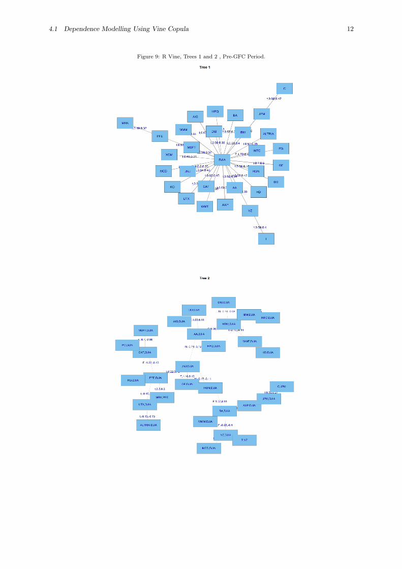
Figure 9: R Vine, Trees 1 and 2 , Pre-GFC Period.


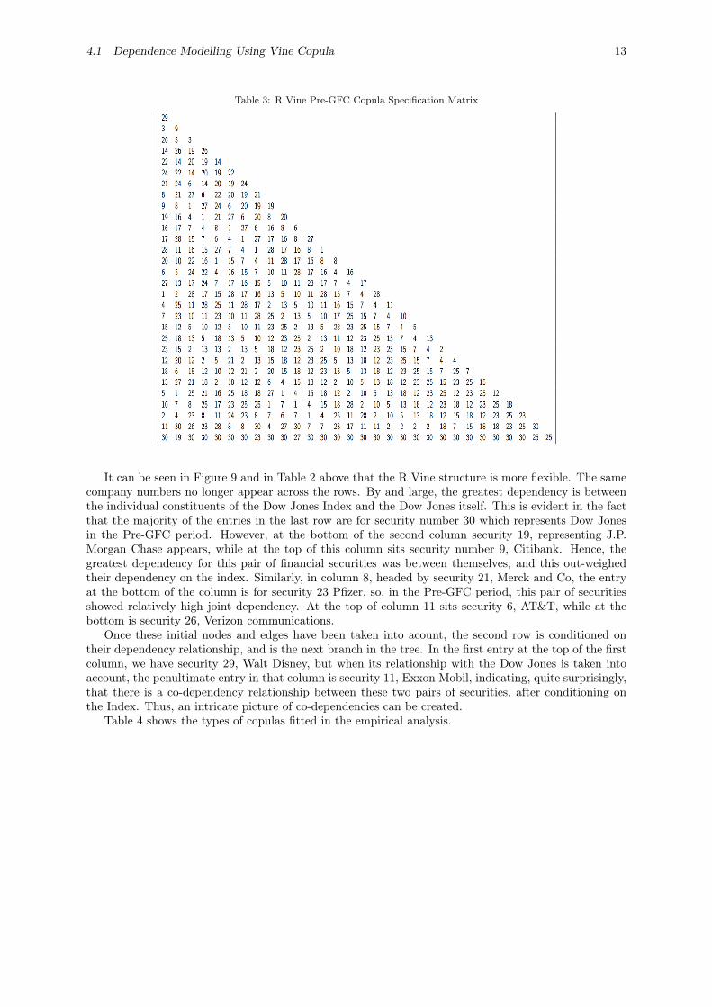
Table 3: R Vine Pre-GFC Copula Specification Matrix

It can be seen in Figure 9 and in Table 2 above that the R Vine structure is more flexible. The samecompany numbers no longer appear across the rows. By and large, the greatest dependency is betweenthe individual constituents of the Dow Jones Index and the Dow Jones itself. This is evident in the factthat the majority of the entries in the last row are for security number 30 which represents Dow Jonesin the Pre-GFC period. However, at the bottom of the second column security 19, representing J.P.Morgan Chase appears, while at the top of this column sits security number 9, Citibank. Hence, thegreatest dependency for this pair of financial securities was between themselves, and this out-weighedtheir dependency on the index. Similarly, in column 8, headed by security 21, Merck and Co, the entryat the bottom of the column is for security 23 Pfizer, so, in the Pre-GFC period, this pair of securitiesshowed relatively high joint dependency. At the top of column 11 sits security 6, AT&T, while at thebottom is security 26, Verizon communications.

Once these initial nodes and edges have been taken into acount, the second row is conditioned ontheir dependency relationship, and is the next branch in the tree. In the first entry at the top of the firstcolumn, we have security 29, Walt Disney, but when its relationship with the Dow Jones is taken intoaccount, the penultimate entry in that column is security 11, Exxon Mobil, indicating, quite surprisingly,that there is a co-dependency relationship between these two pairs of securities, after conditioning onthe Index. Thus, an intricate picture of co-dependencies can be created.

Table 4 shows the types of copulas fitted in the empirical analysis.


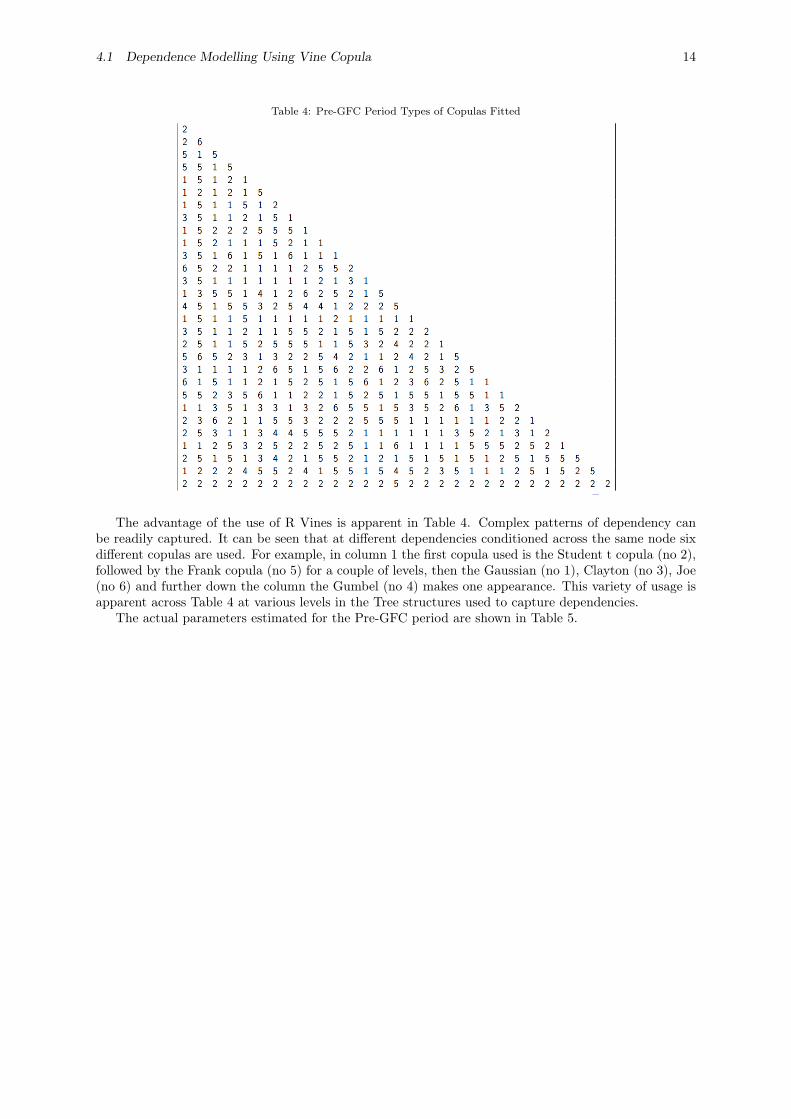
Table 4: Pre-GFC Period Types of Copulas Fitted

The advantage of the use of R Vines is apparent in Table 4. Complex patterns of dependency canbe readily captured. It can be seen that at different dependencies conditioned across the same node sixdifferent copulas are used. For example, in column 1 the first copula used is the Student t copula (no 2),followed by the Frank copula (no 5) for a couple of levels, then the Gaussian (no 1), Clayton (no 3), Joe(no 6) and further down the column the Gumbel (no 4) makes one appearance. This variety of usage isapparent across Table 4 at various levels in the Tree structures used to capture dependencies.

The actual parameters estimated for the Pre-GFC period are shown in Table 5.


Table 5: Pre-GFC Copula Parameter Estimates

If we return to a consideration of the banks in column 2 of Table 5, the strong positive dependenciescan be seen in the values of the entries at the very top and bottom three coefficients in the rows ofcolumn 2.

The key issue for the current analysis is whether these dependencies changed during the GFC andthis is the focus of the next stage of our analysis. Figure 10 shows Trees 1 and 2 for the GFC period.


Figure 10: GFC Period R Vines Trees 1 and 2

There is a change in the groupings in the tree structures produced by the impact of the GFC. Citibankis absent from the list because it had to be rescued by the US Government under plans agreed for Citi-Group, following large losses in the value of its subprime mortgage assets. The remaining major financial


services companies are grouped together, J.P. Morgan and American Express, together with the aviationand defence sector companies United Technologies and Boeing. Similarly, the IT companies, Intel, Mi-crosoft, Hewlett Packard and IBM, are grouped together, as are the main-stream consumer products andindustrial groupings, Coca-Cola, Proctor and Gamble, Johnson and Johnson. Drug companies Merckand Pfizer, and communications giants Verizon and AT&T are linked. A final chain is provided byGeneral Electric, 3M and Alcoa.

The details of the linkages in the tree structures and the nature of the dependencies in the GFCperiod are provided in Table 6.

Table 6: R Vine GFC Copula Specification Matrix

The picture and tree structures are changed dramatically by the GFC. At the top of the first columnsits United Technologies (no 22 in the GFC set), paired with the Dow Jones (no 26). The next link in thetree is with Boeing (no 5) sitting next to the bottom of the column, followed by J.P. Morgan Chase (no15). This segment of Tree 2 can be seen in the bottom right of Figure 10. Column 3 is dominated by thelinks between Verizon (no 23) and AT&T (no 4). The other column in which the strongest dependency isnot on the index is column 13, in which Merck (no 17) sits at the top with Pfizer (no 19) at the bottom.This linkage is shown in the middle of the right-hand side of the diagram for Tree 2 in Figure 10. Allthe other remaining dominating dependencies are with the Dow Jones Index.

The specification of the copula types fitted during the GFC are presented in Table 7.


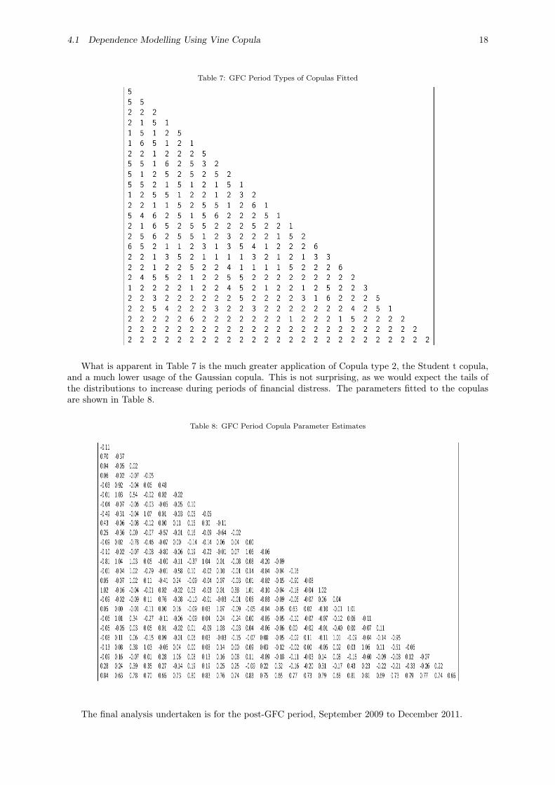
Table 7: GFC Period Types of Copulas Fitted

What is apparent in Table 7 is the much greater application of Copula type 2, the Student t copula,and a much lower usage of the Gaussian copula. This is not surprising, as we would expect the tails ofthe distributions to increase during periods of financial distress. The parameters fitted to the copulasare shown in Table 8.

Table 8: GFC Period Copula Parameter Estimates

The final analysis undertaken is for the post-GFC period, September 2009 to December 2011.


Figure 11: Post-GFC Period R Vines Trees 1 and 2

The industry groupings are apparent in Tree 2, shown in Figure 11. There is an IT cluster featuringMicrosoft, Intel, Cisco and Hewlett Packard, and a financial services cluster which includes Bank ofAmerica, American Express, Travellers Co and J.P. Morgan. The drug companies group together in


the dependencies shown between Pfizer, Merck and Johnson and Johnson. Oil, retail companies andmanufacturing companies are spread about.

Table 9 shows the copulas specification matrix for the Post-GFC period.

Table 9: Post-GFC R Vine Copula Specification Matrix

If we look first at the cases of strong dependencies that are not initially partnered with the DowJones Index at the top of column one in Table 9, we have Exxon Mobil (no 11) at the top and Chevron(no 8) at the bottom, revealing strong co-dependencies between these two major oil companies. Bank ofAmerica (no 5) is at the top of column six and J.P. Morgan Chase (no 18), is at the bottom. Verizon (no28) is at the top of column eleven and AT&T (no 4), is at the bottom, revealing the linkages betweenthese two communications companies. All the other companies are linked via their relationship with theDow Jones Index (no 31), which appears as the bottom entry in most of the columns.

The copulas fitted in the Post-GFC period are shown in Table 10.


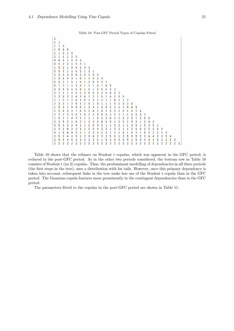
Table 10: Post-GFC Period Types of Copulas Fitted

Table 10 shows that the reliance on Student t copulas, which was apparent in the GFC period, isreduced in the post-GFC period. As in the other two periods considered, the bottom row in Table 10consists of Student t (no 2) copulas. Thus, the predominant modelling of dependencies in all three periods(the first steps in the tree), uses a distribution with fat tails. However, once this primary dependency istaken into account, subsequent links in the tree make less use of the Student t copula than in the GFCperiod. The Gaussian copula features more prominently in the contingent dependencies than in the GFCperiod.

The parameters fitted to the copulas in the post-GFC period are shown in Table 11.

4.2 Empirical Example 22

Table 11: Post-GFC Period Copula Parameter Estimates

4.2. Empirical ExampleThe multivariate dependence structure obtained from R-Vine Copulas can be used for portfolio eval-

uation and risk modelling. The R-Vine approach potentially gives better results than usual bivariatecopula approach as the copulas selected via Vine copulas are more sensitive to the asset’s return distri-bution. Table-12 gives the Copula Kendall Tau’s for the GFC period in our sample data, the results intable-12 are visualized in figure-12. Its evident that the dependence across assets varies.

Table 12: R-Vine Tau Matrix (GFC Period)

4.2 Empirical Example 23

Figure 12: Tau Matrix Plot (GFC Period)

The co-dependencies calculated by R-Vine copulas can be used for portfolio Value at Risk quantifica-tion. We construct an equally weighted portfolio of ten DJIA stocks (including DJIA) to illustrate the useof Vine copulas in modelling VaR using a portfolio example. The data used for this part of the analysisis from 3-Jan-2010 to 31-Dec-2011 with total 504 returns per asset, the ten arbitrarily selected assetsin the portfolio are; DJIA, Alcoa, General Electric, Johnson & Johnson, Microsoft, American Express,P&G, Boeing and Home Depot. We use a 250 days moving window dynamic approach to forecast theVaR for this equally weighted portfolio which results in 254 forecasts. The main steps of the approachare as outlined below:

1. Convert the data sample to log returns.2. Select a moving window of 250 returns.3. Fit GARCH(1,1) with Student-t innovations to convert the log returns into an i.i.d. series. We fit

the same GARCH(1,1) with student-t in all the iterations to maintain uniformity in the method,and this approach also makes the method a little less computationally intensive.

4. Extract the residuals from Step-3 and standardize them with the Standard deviations obtainedfrom Step-3.

5. Convert the standardized residuals to student-t marginals for Copula estimation. The steps aboveare repeated for all the 10 stocks to obtain a multivariate matrix of uniform marginals.

6. Fit an R-Vine to the multivariate data with the same copulas as used in Section-1.7. Generate simulations using the fitted R-Vine model. We generate 1000 simulations per stock for

forecasting a day ahead VaR.8. Convert the simulated uniform marginals to standardized residuals.9. Simulate returns from the simulated standardized residuals using GARCH simulations.10. Generate a series of simulated daily portfolio returns to forecast 1% and 5% VaR.11. Repeat step 1 to 10 for a moving window.

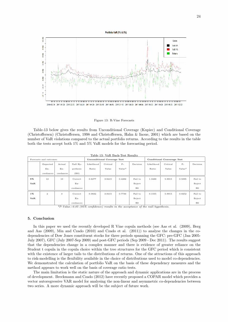
The approach above results in VaR forecasts which whilst not dependent in time have the advantageof being co-dependent on the stocks in the portfolio. We uses this approach as a demonstration of apractical application of the information about co-dependencies captured by the flexible Vine Copulaapproach applied to generate a frequently applied risk metric. Figure-13 plots the 1% and 5% VaRforecasts along with original portfolio return series obtained from the method. The plot shows that theVaR forecasts closely follow the daily returns with few violations.

24

Figure 13: R-Vine Forecasts

Table-13 below gives the results from Unconditional Coverage (Kupiec) and Conditional Coverage(Christoffersen) (Christoffersen, 1998 and Christoffersen, Hahn & Inoue, 2001) which are based on thenumber of VaR violations compared to the actual portfolio returns. According to the results in the tableboth the tests accept both 1% and 5% VaR models for the forecasting period.

Table 13: VaR Back-Test ResultsForecasts and outcomes Unconditional Coverage Test Conditional Converage Test

Expected

Ex-

ceedances

Actual

Ex-

ceedances

Null Hy-

pothesis

(H0)

Likelihood

Ratio

Critical

Value

P-

Value*

Decision Likelihood

Ratio

Critical

Value

P-

Value*

Decision

5%

VaR

12 10 Correct

Ex-

ceedances

0.6277 3.8415 0.4282 Fail to

Reject

H0

1.3488 5.9915 0.5095 Fail to

Reject

H0

1%

VaR

2 3 Correct

Ex-

ceedances

0.0832 3.8415 0.7730 Fail to

Reject

H0

0.1555 5.9915 0.9252 Fail to

Reject

H0

*P-Value>0.05 (95% confidence) results in the acceptance of the null hypothesis.

5. Conclusion

In this paper we used the recently developed R Vine copula methods (see Aas et al. (2009), Bergand Aas (2009), Min and Czado (2010) and Czado et al. (2011)) to analyse the changes in the co-dependencies of Dow Jones constituent stocks for three periods spanning the GFC: pre-GFC (Jan 2005-July 2007), GFC (July 2007-Sep 2009) and post-GFC periods (Sep 2009 - Dec 2011). The results suggestthat the dependencies change in a complex manner and there is evidence of greater reliance on theStudent t copula in the copula choice within the tree structures for the GFC period which is consistentwith the existence of larger tails to the distributions of returns. One of the attractions of this approachto risk-modelling is the flexibility available in the choice of distributions used to model co-dependencies.We demonstrated the calculation of portfolio VaR on the basis of these dependency measures and themethod appears to work well on the basis of coverage ratio tests.

The main limitation is the static nature of the approach and dynamic applications are in the processof development. Breckmann and Czado (2012) have recently proposed a COPAR model which provides avector autoregressive VAR model for analysing the non-linear and asymmetric co-dependencies betweentwo series. A more dynamic approach will be the subject of future work.

25

Acknowledgement: For financial support, the authors wish to thank the Australian ResearchCouncil. The third author would also like to acknowledge the National Science Council, Taiwan,and the Japan Society for the Promotion of Science. The authors thank the reviewers forhelpful comments.

26

References

[1] Aas, K., C. Czado, A. Frigessi and H. Bakken (2009) “Pair-copula constructions of multipledependence”, Insurance, Mathematics and Economics, 44, 182–198.

[2] Bedford, T. and R. M. Cooke (2001) “Probability density decomposition for conditionallydependent random variables modeled by vines”, Annals of Mathematics and Articial Intel-ligence 32, 245-268.

[3] Bedford, T. and R. M. Cooke (2002) “Vines - a new graphical model for dependent randomvariables”, Annals of Statistics 30, 1031-1068.

[4] Berg, D., (2009) “Copula goodness-of-fit testing: an overview and power comparison”, TheEuropean Journal of Finance, 15:675–701.

[5] Berg, D., and K. Aas, (2009) “Models for construction of higher-dimensional dependence:A comparison study”, European Journal of Finance, 15:639–659.

[6] Brechmann, E. C., C. Czado, and K. Aas, (2012) “Truncated regular vines and their appli-cations”, Canadian Journal of Statistics 40 (1), 68-85.

[7] Brechmann, E.C., and U. Schepsmeier, (2012) “Modeling dependencewith C- and D-vine copulas” The R-package CDVine, http://cran.r-project.org/web/packages/CDVine/vignettes/CDVine-package.pdf

[8] Brechmann, E. C., and C. Czado (2012) “COPAR - multivariate time-series modelling usingthe COPula AutoRegressive model”, Working Paper, Faculty of Mathematics, TechnicalUniversity of Munich.

[9] Chollete, L., Heinen, A., and A. Valdesogo, (2009) “Modeling international financial returnswith a multivariate regime switching copula”, Journal of Financial Econometrics, 7:437–480.

[10] Christoffersen, P., (1998) “Evaluating Interval Forecasts”, International Economic Review,39, 841–862.

[11] Christoffersen, P., J. Hahn, and A. Inoue, (2001) ‘‘Testing and Comparing Value-at-RiskMeasures’’, Journal of Empirical Finance, 8, 325–342.

[12] Cooke, R.M., H. Joe and K. Aas, (2011) “Vines Arise”, chapter 3 in DEPENDENCE MOD-ELING Vine Copula Handbook, Ed. D. Kurowicka and H. Joe, World Scientific PublishingCo, Singapore.

[13] Czado, C., U. Schepsmeier, and A. Min (2011) “Maximum likelihood estimation of mixedC-vines with application to exchange rates”. To appear in Statistical Modelling.

[14] Dimann, J., E. C. Brechmann, C. Czado, and D. Kurowicka (2012) “Selecting and es-timating regular vine copulae and application to financial returns”, Submitted preprint.http://arxiv.org/abs/1202.2002.

[15] Dissman, J.F. (2010) Statistical Inference for Regular Vines and Application, Thesis, Tech-nische Universitat Munchen, Zentrum Mathematik.

[16] Heinen, A. and A. Valdesogo (2009) “Asymmetric CAPM dependence for large dimen-sions: the canonical vine autoregressive model”, CORE discussion papers 2009069, Univer-site catholique de Louvain, Center for Operations Research and Econometrics (CORE).

[17] Joe, H., (1996) “Families of m-variate distributions with given margins and m(m- 1)/2bivariate dependence parameters”. In L. Rüschendorf and B. Schweizer and M. D. Taylor,editor, Distributions with Fixed Marginals and Related Topics.

[18] Joe, H. (1997) Multivariate Models and Dependence Concepts. Chapman & Hall, London.

[19] Joe, H., Li, H., and A. Nikoloulopoulos, (2010) “Tail dependence functions and vine copulas”,Journal of Multivariate Analysis, 101(1):252–270.

27

[20] Kullback, S. and R.A. Leibler, (1951) “On information and sufficiency”, The Annals ofMathematical Statistics, 22(1):79–86.

[21] Kupiec, P., (1995) ‘‘Techniques for verifying the accuracy of risk measurement models’’,Journal of Derivatives 3, 73-84.

[22] Kurowicka, D., (2011) “Optimal truncation of vines”, In D. Kurowicka and H. Joe (Eds.),Dependence Modeling: Handbook on Vine Copulae. Singapore: World Scientific PublishingCo.

[23] Kurowicka D. and R.M. Cooke, (2003) “A parametrization of positive definite matrices interms of partial correlation vines”, Linear Algebra and its Applications, 372, 225–251.

[24] Kurowicka, D. and R. M. Cooke, (2006) “Uncertainty Analysis with High DimensionalDependence Modelling”, Chichester: John Wiley.

[25] Mendes, B. V. d. M., M. M. Semeraro, and R. P. C. Leal, (2010) “Pair-copulas modeling infinance”, Financial Markets and Portfolio Management 24, 193-213.

[26] Min, A., and C. Czado, (2010) “Bayesian inference for multivariate copulas using pair-copulaconstructions”, Accepted for publication in Journal of Financial Econometrics.

[27] Morales-N´apoles, O., R. Cooke, and D. Kurowicka (2009) “About the number of vines andregular vines on n nodes”, Submitted to Linear Algebra and its Applications.

[28] Nelsen, R., (2006) An Introduction to Copulas, Springer, New York, 2nd edition.

[29] Patton, A. J., (2009) “Copula based models for financial time series”, in: Handbook ofFinancial Time Series. pp. 767-785

[30] Prim, R. C., (1957) “Shortest connection networks and some generalizations”, Bell SystemTechnical Journal, 36:1389–1401.

[31] Schirmacher, D. and E. Schirmacher, (2008) “Multivariate dependence mod-eling using pair-copulas”, Technical report, Society of Actuaries: 2008 En-terprise Risk Management Symposium, April 14-16, Chicago. Available from:http://www.soa.org/library/monographs/other-monographs/2008/april/ 2008-erm-toc.aspx

[32] Sklar, A., (1959) “Fonctions de repartition a n dimensions et leurs marges”, Publications del’Institut de Statistique de L’Universite de Paris 8, 229-231.

[33] Smith, M., Min, A., C. Czado, C., and C. Almeida, (2010) “Modeling longitudinal datausing a pair-copula decomposition of serial dependence”, In revision for the Journal of theAmerican Statistical Association.

[34] Vuong, Q. H., (1989) “Likelihood ratio tests for model selection and non-nested hypotheses”,Econometrica, 57:307–333.

financial dependence analysis: applications of … dependence analysis: applications of vine copulas...

Documents