www.SandV.com8 SOUND & VIBRATION/MARCH 2011

With the unrestricted release of MIL-STD-810G, which includes Method 527 – Multi-Exciter Testing, there is more interest than ever in performing vibration tests that involve using more than one shaker. Also, in the tradition of earlier releases of MIL-STD-810, use of actual measured field data is encouraged wherever pos-sible. While it is acknowledged that tailoring of measured data will probably be required and a modal survey of the proposed test setup is desirable, many of the steps required to use field data have not been fully reported. This article examines some of the detailed requirements for using measured data to perform a multi-exciter random vibration test in the laboratory. Using MIL-STD-810G and IEST Committee DTE-022 as background, measurements that can be transformed into a four-shaker test will be used as an example. While both time waveform replication and random multishaker tests can be established from measured field data, we concentrate on the methodology associated with such random tests. Using power and cross-spectral densities from measured field data, the entire system spectral density matrix is filled to completely define the field vibration environment. Test results are compared with field measurements and suggestions made as to potential recom-mended steps needed to assure a successful field simulation.

As the use of multiple shakers to excite a single structure in-creases, there has been much discussion about optimum ways to configure such tests and provide the best possible control.1 And as the number and size of shakers increases, we find ourselves conducting multiple-input-multiple-output (MIMO) tests with incredibly large force levels at our disposal.1 Yet we know that when all is said and done, we cannot force a structure to move in ways that are unnatural no matter how hard we try.1 So no matter how we arrive at the test requirements, we need to be sure that the test setup represents an achievable configuration, hopefully related to field conditions, and that the test control philosophy is based on a rigorous, mathematically correct approach.1

As the repercussions of MIL-STD-810G2 spread and more test-ing organizations begin to consider using multiple shakers for the first time, we need guidance from the most experienced test engi-neers. Many of these engineers are contributing to a recommended practice (RP) that is being developed under the auspices of IEST Committee DTE-022. One of the key premises included in this RP is that experience has shown that the entire test system, including shakers, amplifiers, fixtures, test articles, transducers, cables, etc., must be taken into account to achieve a successful MIMO test. The only sure way to achieve this is to define the entire system as a frequency response matrix (FRM), measure this FRM before the test begins, and continuously control and update this matrix on a real-time basis as the test progresses.3,4 This is the only techni-cally robust way to assure that magnitude, phase, coherence and cross-coupling compensation are achieved in a correct, logical and mathematically rigorous way.1

One way of describing a four-shaker test is to visualize the rela-tionships between the desired Control vectors, the Drive vectors necessary to produce this control and the set of frequency response functions, which is the FRM of the system under test, that relate all the Drive inputs and Control responses in our test system. A matrix representation of this four-shaker system, with the use of the FRM: [H(f)], looks like:

where:{C(f)} = vector of Control Fourier spectra{D(f)} = vector of Drive Fourier spectra{H(f)} = matrix of FRFs between Control i and Drive j

Important ConceptsThis article presents results obtained with the use of data form-•ing a measured spectral density matrix (SDM) as the Reference for a multishaker test.5

The SDM is meant to represent measured field data that de-•scribes the vibration present on a structure due to its service environment.1,2,5

Filling in the MIMO MatrixPart 1 – Performing Random Tests Using Field Data

(1)

c f

c f

c f

c f

h f h f h f h1

2

3

4

11 12 13 1( )

( )

( )

( )

( ) ( ) ( )Ï

ÌÔÔ

ÓÔÔ

¸

˝ÔÔ

˛ÔÔ

=

44

21 22 23 24

31 32 33 34

( )

( ) ( ) ( ) ( )

( ) ( ) ( ) (

f

h f h f h f h f

h f h f h f h f

))

( ) ( ) ( ) ( )

( )

( )

( )

h f h f h f h f

d f

d f

d f

41 42 43 44

1

2

3

È

Î

ÍÍÍÍÍ

˘

˚

˙˙˙˙˙ dd f4( )

Ï

ÌÔÔ

ÓÔÔ

¸

˝ÔÔ

˛ÔÔ

Marcos Underwood, Russ Ayres, and Tony Keller, Spectral Dynamics, Inc., San Jose, California

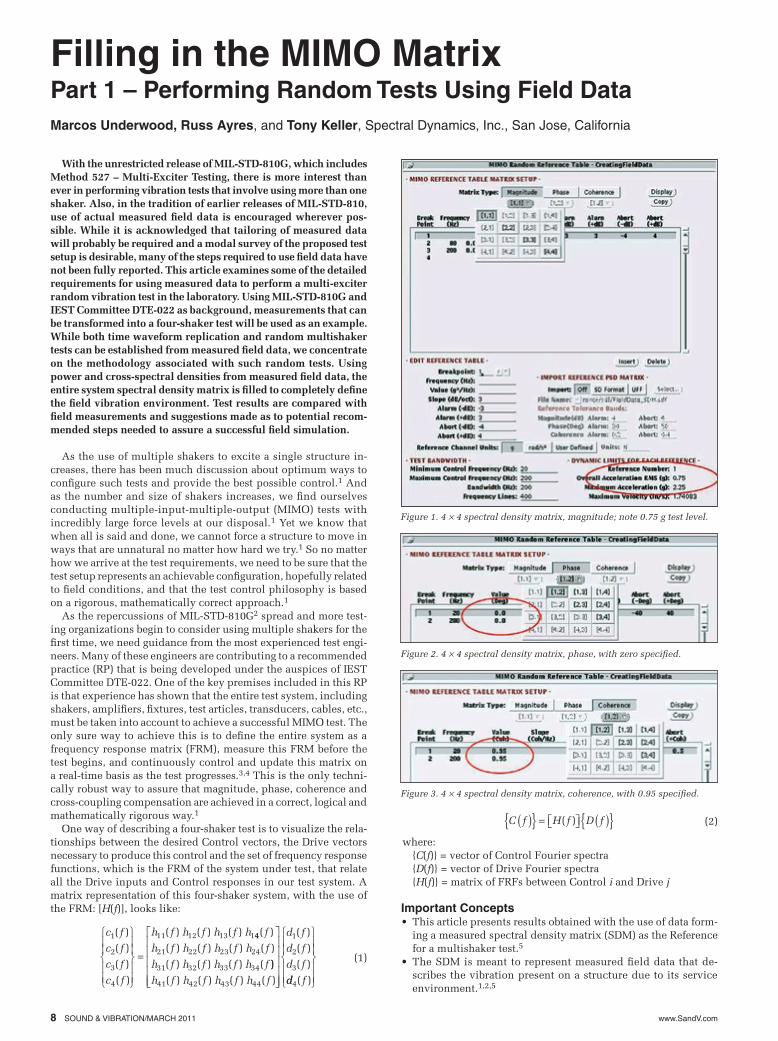
Figure 2. 4 ¥ 4 spectral density matrix, phase, with zero specified.

Figure 3. 4 ¥ 4 spectral density matrix, coherence, with 0.95 specified.

(2)C f H f D f( ){ } = ÈÎ ˘̊ ( ){ }( )

Figure 1. 4 ¥ 4 spectral density matrix, magnitude; note 0.75 g test level.

www.SandV.com SOUND & VIBRATION/MARCH 2011 9

Using this SDM as a test’s reference, a MIMO random approach •can be used to reproduce this measured field environment in the lab.2,5

The major advantage of using this methodology, versus repli-•cation, for example, is that this test will visit all the vibration states according to a Gaussian distribution and in an ergodic sense.1,5 If the field boundary conditions are suitably simulated in the •lab, the study also shows that responses on other noncontrolled parts of the structure will also respond in a manner that is quite similar to what is observed in the field. This is a result of the advanced technology that is used to control all elements of the structure’s response SDM to ensure it agrees acceptably with the SDM that was measured in the field.

Defining the TestIn the example used here, a plate driven by four electrodynamic

shakers will be employed. To create the most straightforward Control situation, four Control points are used to create a “square” control configuration. If we are to use measured, continuous, field data as the basis for the test, the system matrix for this test will have the form shown in Figure 1.

In this example, the four PSD (power spectral density) terms of the major diagonal are highlighted. If a test is being defined by separately entering PSD profiles, associated phase and desired coherence, then after entering the PSDs, which have magnitude values only, along the major diagonal, additional data must be entered. For example, the required phase profiles would be entered as shown in Figure 2.

The profiles for the test phase have the form seen in Figure 3. This fills in the upper off-diagonal matrix elements with the required Hermitian symmetry between the upper and lower off-diagonal elements enforced.1,5 So for a four-exciter system, we will need to define four PSDs but six profiles for phase and six profiles for coherence. In this example, where we start by defining and entering reference profiles for magnitude, phase and coherence, we would let the control system calculate the reference cross-spectral densi-ties. So we actually set up the references for the test as:

where:[GRR(f)] = reference spectral density matrixgnn(f) = reference power spectral densitygnm(f) = reference cross spectral densityFor the current test, the first four-shaker test setup is shown in

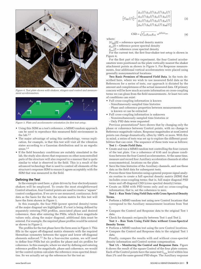
Figure 4.For the first part of this experiment, the four Control acceler-

ometers were positioned on the plate vertically nearest the shaker attachment points as shown in Figure 5. For Response measure-ments, four additional vertical accelerometers were placed using generally nonsymmetrical locations.

Two Basic Premises of Measured Field Data. In the tests de-scribed here, where we wish to use measured field data as the References for a series of tests, our approach is dictated by the amount and completeness of the actual measured data. Of primary concern will be how much accurate information on cross-coupling terms we can glean from the field measurements. At least two sets of conditions can exist:

Full cross-coupling information is known•- Simultaneously sampled time histories- Phase and coherence properties between measurements is known or can be extractedFull cross-coupling information is unknown•- Nonsimultaneously sampled time histories or- Only PSD data were requestedPrevious presentations6 have shown that by changing only the

phase or coherence between Control points, with no change to Reference magnitude values, Response magnitudes at nonControl points can change dramatically, often by 100% or more. With this in mind, a series of tests was set up to explore the different possi-bilities that can exist. The sequence of these tests was as follows:

Test 1 – Create Field Data.Create and run a MIMO random test controlling the four corners •of the test plate. Use a coherence of 0.95 and in-phase condi-tions between the four Control accelerometers. At the same time, measure and record four Auxiliary acceleration channels at other nonsymmetrical, locations on the plate.Save the time histories of the Auxiliary channels, and use these •data as the field data for subsequent tests.Process these time histories using a general purpose signal analy-•sis routine to create a full spectral density matrix (SDM) that includes cross-coupling terms; that is, full major diagonal PSD terms and off-diagonal CSD (cross spectral density) terms.Create an SDM with PSD terms only and no cross-coupling •information; that is, set the coherence to zero.Test 2 – Run Tests Using Field Data with Cross Spectral Density

Terms.Perform a MIMO random test using new Control locations that •correspond to the Auxiliary measurement locations from Test 1.Compare the Control and Response data to the original Test 1 •data.Check for dynamic reciprocity between Test 1 and Test 2.•Test 3 – Run Tests Using Field Data without Cross-Spectral

Density Terms.Perform a MIMO random test using the new Control locations.•Compare the Control and Response data to the original Test 1 •data.Finally, compare the results with and without cross-spectral

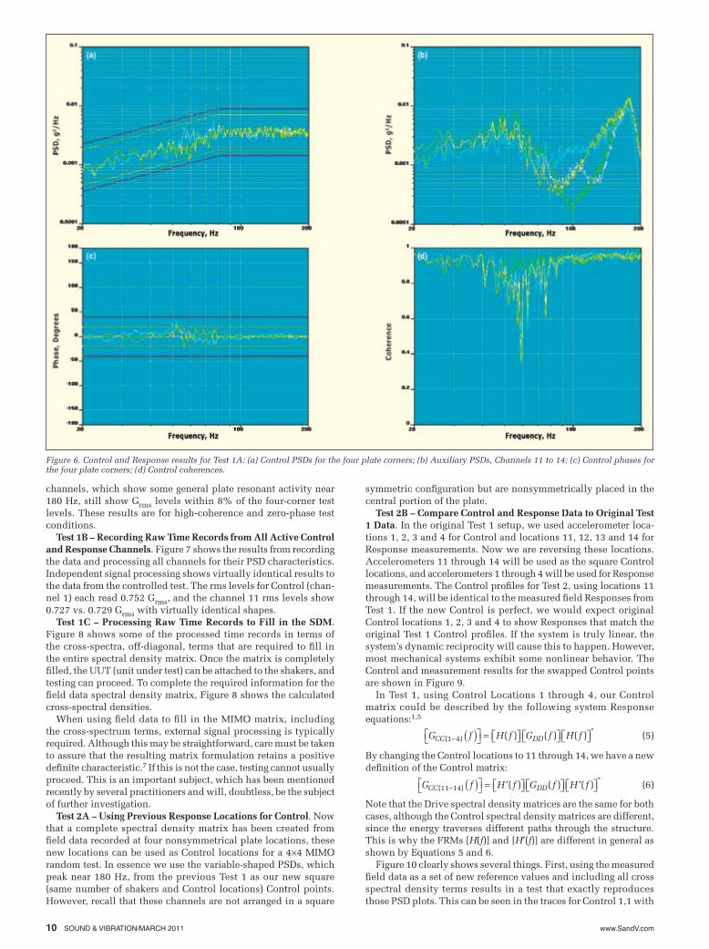
density information and Control system compensation. Test 1A – Monitoring the Control and Response Data. Figure

6 shows the result of the square Control of the four plate corners. Each of the Control points have the same test Grms level within less than 2% and the same general PSD shape. The Auxiliary response

Figure 5. Plate and accelerometer orientation for first test setup.

Figure 4. Test plate shown with shakers, stingers and control and measure-ment accelerometers.

(3)G f

g f g f g f g f

g f g f g fRR ( )ÈÎ ˘̊ =

11 12 13 14

21 22 23

( ) ( ) ( ) ( )

( ) ( ) ( )

g f

g f g f g f g f

g f g f g f g

24

31 32 33 34

41 42 43 4

( )

( ) ( ) ( ) ( )

( ) ( ) ( ) 44( )f

È

Î

ÍÍÍÍÍ

˘

˚

˙˙˙˙˙

CSD = g mn mm nniphaseg g e mn2

(4)

www.SandV.com10 SOUND & VIBRATION/MARCH 2011

channels, which show some general plate resonant activity near 180 Hz, still show Grms levels within 8% of the four-corner test levels. These results are for high-coherence and zero-phase test conditions.

Test 1B – Recording Raw Time Records from All Active Control and Response Channels. Figure 7 shows the results from recording the data and processing all channels for their PSD characteristics. Independent signal processing shows virtually identical results to the data from the controlled test. The rms levels for Control (chan-nel 1) each read 0.752 Grms, and the channel 11 rms levels show 0.727 vs. 0.729 Grms with virtually identical shapes.

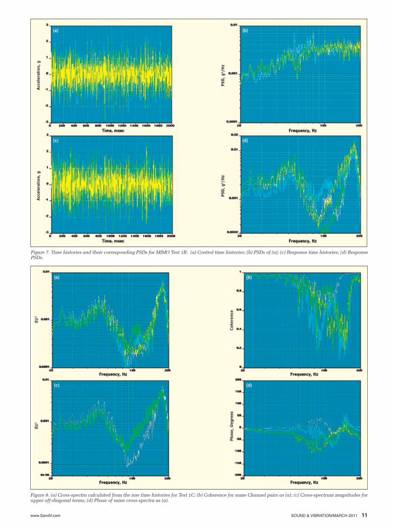
Test 1C – Processing Raw Time Records to Fill in the SDM. Figure 8 shows some of the processed time records in terms of the cross-spectra, off-diagonal, terms that are required to fill in the entire spectral density matrix. Once the matrix is completely filled, the UUT (unit under test) can be attached to the shakers, and testing can proceed. To complete the required information for the field data spectral density matrix, Figure 8 shows the calculated cross-spectral densities.

When using field data to fill in the MIMO matrix, including the cross-spectrum terms, external signal processing is typically required. Although this may be straightforward, care must be taken to assure that the resulting matrix formulation retains a positive definite characteristic.7 If this is not the case, testing cannot usually proceed. This is an important subject, which has been mentioned recently by several practitioners and will, doubtless, be the subject of further investigation.

Test 2A – Using Previous Response Locations for Control. Now that a complete spectral density matrix has been created from field data recorded at four nonsymmetrical plate locations, these new locations can be used as Control locations for a 4¥4 MIMO random test. In essence we use the variable-shaped PSDs, which peak near 180 Hz, from the previous Test 1 as our new square (same number of shakers and Control locations) Control points. However, recall that these channels are not arranged in a square

symmetric configuration but are nonsymmetrically placed in the central portion of the plate.

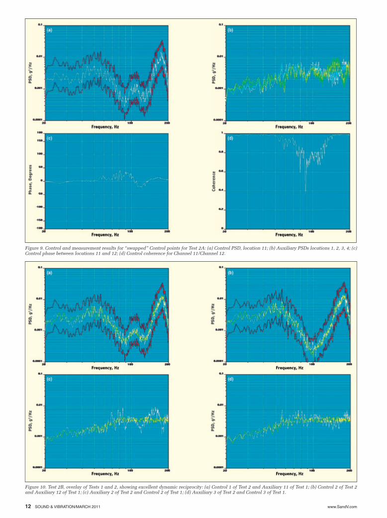
Test 2B – Compare Control and Response Data to Original Test 1 Data. In the original Test 1 setup, we used accelerometer loca-tions 1, 2, 3 and 4 for Control and locations 11, 12, 13 and 14 for Response measurements. Now we are reversing these locations. Accelerometers 11 through 14 will be used as the square Control locations, and accelerometers 1 through 4 will be used for Response measurements. The Control profiles for Test 2, using locations 11 through 14, will be identical to the measured field Responses from Test 1. If the new Control is perfect, we would expect original Control locations 1, 2, 3 and 4 to show Responses that match the original Test 1 Control profiles. If the system is truly linear, the system’s dynamic reciprocity will cause this to happen. However, most mechanical systems exhibit some nonlinear behavior. The Control and measurement results for the swapped Control points are shown in Figure 9.

In Test 1, using Control Locations 1 through 4, our Control matrix could be described by the following system Response equations:1,5

By changing the Control locations to 11 through 14, we have a new definition of the Control matrix:

Note that the Drive spectral density matrices are the same for both cases, although the Control spectral density matrices are different, since the energy traverses different paths through the structure. This is why the FRMs [H(f)] and [H¢(f)] are different in general as shown by Equations 5 and 6.

Figure 10 clearly shows several things. First, using the measured field data as a set of new reference values and including all cross spectral density terms results in a test that exactly reproduces those PSD plots. This can be seen in the traces for Control 1,1 with

Figure 6. Control and Response results for Test 1A: (a) Control PSDs for the four plate corners; (b) Auxiliary PSDs, Channels 11 to 14; (c) Control phases for the four plate corners; (d) Control coherences.

(5)G f H f G f H fCC DD( )*

( ) ( ) ( )1 4- ( )ÈÎ ˘̊ = ÈÎ ˘̊ ÈÎ ˘̊ ÈÎ ˘̊

(6)G f H f G f H fCC DD( )*

( ) ( ) ( )11 14- ( )ÈÎ ˘̊ = ¢ÈÎ ˘̊ ÈÎ ˘̊ ¢ÈÎ ˘̊

www.SandV.com SOUND & VIBRATION/MARCH 2011 11

Figure 7. Time histories and their corresponding PSDs for MIMO Test 1B: (a) Control time histories; (b) PSDs of (a); (c) Response time histories; (d) Response PSDs.

Figure 8. (a) Cross-spectra calculated from the raw time histories for Test 1C; (b) Coherence for same Channel pairs as (a); (c) Cross-spectrum magnitudes for upper off-diagonal terms; (d) Phase of same cross-spectra as (a).

www.SandV.com12 SOUND & VIBRATION/MARCH 2011

Figure 9. Control and measurement results for “swapped” Control points for Test 2A: (a) Control PSD, location 11; (b) Auxiliary PSDs locations 1, 2, 3, 4; (c) Control phase between locations 11 and 12; (d) Control coherence for Channel 11/Channel 12.

Figure 10. Test 2B, overlay of Tests 1 and 2, showing excellent dynamic reciprocity: (a) Control 1 of Test 2 and Auxiliary 11 of Test 1; (b) Control 2 of Test 2 and Auxiliary 12 of Test 1; (c) Auxiliary 2 of Test 2 and Control 2 of Test 1; (d) Auxiliary 3 of Test 2 and Control 3 of Test 1.

www.SandV.com SOUND & VIBRATION/MARCH 2011 13

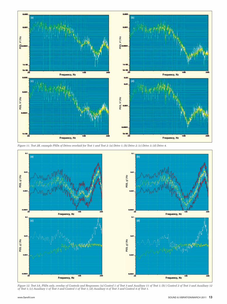
Figure 11. Test 2B, example PSDs of Drives overlaid for Test 1 and Test 2: (a) Drive 1; (b) Drive 2; (c) Drive 3; (d) Drive 4.

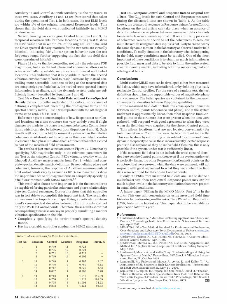
Figure 12. Test 3A, PSDs only, overlay of Controls and Responses: (a) Control 1 of Test 3 and Auxiliary 11 of Test 1; (b) ) Control 2 of Test 3 and Auxiliary 12 of Test 1; (c) Auxiliary 1 of Test 3 and Control 1 of Test 1; (d) Auxiliary 4 of Test 3 and Control 4 of Test 1.

www.SandV.com14 SOUND & VIBRATION/MARCH 2011

Table 1. Measured Grms for three test conditions.

Test No. Location Control Location Response Error, %

1 1 0.749 11 0.728 – 2 0.735 12 0.774 – 3 0.751 13 0.713 – 4 0.740 14 0.805 –

2 11 0.728 1 0.787 5.07 12 0.776 2 0.780 6.12 13 0.717 3 0.770 2.53 14 0.807 4 0.760 2.70

3 11 0.713 1 1.617 115.89 12 0.750 2 1.919 161.09 13 0.705 3 11.008 34.22 14 0.802 4 1.424 92.43

Auxiliary 11 and Control 3,3 with Auxiliary 13, the top traces. In these two cases, Auxiliary 11 and 13 are from stored data taken during the operation of Test 1. In both cases, the test RMS levels are within 1% of the original measured Response levels. This shows that the field data were replicated faithfully in a MIMO random sense.

Second, looking back at original Control Locations 1 and 3, the reciprocal measurements for these locations during Test 2, show an RMS value that is within 5% of the original PSD data. And the Drive spectral density matrices for the two tests are virtually identical, indicating fairly linear system behavior over the test frequency range, further supporting the fact that the field data were reproduced faithfully.

Figure 11 shows that by controlling not only the reference PSD magnitudes, but also the test phase and coherence, allows us to achieve virtually repeatable, reciprocal conditions at nonControl locations. This indicates that it is possible to create the needed vibration environment at hard-to-reach locations by instead con-trolling more accessible locations as long as the measured data are completely specified; that is, the needed cross-spectral density information is available, and the dynamic system paths are suf-ficiently linear (described by Equations 5 and 6).

Test 3A – Run Tests Using Field Data without Cross-Spectral Density Terms. To better understand the critical importance of defining a complete test, including the off-diagonal terms of the spectral density matrix, Test 2 was repeated with the off-diagonal terms set to zero. This is Test 3.

Reference 6 gives some examples of how Responses at nonCon-trol locations on a test structure can vary widely even if slight changes are made to the phase or coherence between Control loca-tions, which can also be inferred from (Equations 4 and 5). Such results will occur on a highly resonant system when the relative coherence is arbitrarily set to zero, as in this case, which creates in essence a free-phase situation that is different than what existed as part of the measured field environment.

The results of just such a test are seen in Figure 12. Note that by specifying PSD magnitudes only in the reference parameters for the Test 3, the (shaped) Control PSDs virtually overlay with the (shaped) Auxiliary measurements from Test 1, which had com-plete spectral density matrix definition. By not defining phase and coherence, however, the response of Auxiliary measurements at nonControl points vary by as much as 161%. So these results show the importance of the off-diagonal terms in completely specifying a field environment with MIMO random.1,5

This result also shows how important it is for the controller to be capable of forcing particular coherence and phase relationships between Control responses. Our results show that this controller was in fact able to accomplish this important task. The result also underscores the importance of specifying a particular environ-ment’s cross-spectral densities between Control points and not only the PSDs at Control points. Therefore, these results show that accomplishing two tasks are key in properly simulating a random vibration specification in the lab:

Completely specifying the environment’s spectral density •matrix.Having a capable controller conduct the MIMO random test.•

Test 3B – Compare Control and Response Data to Original Test 1 Data. The Grms levels for each Control and Response measured during the discussed tests are shown in Table 1. As the table shows, the greatest divergence in Response values for nonControl locations on the test article can take place when an absence of data for coherence or phase between measured data channels forces us to take an alternate approach. If we arbitrarily pick a set of coherence values or decide to set the coherences to zero, our multishaker test using field data inputs is not likely to create nearly the same dynamic motion in the laboratory as observed under field conditions. To really simulate in the laboratory what is happening in the field, many conditions must be satisfied. One of the most important of these conditions is to obtain as much information as possible from measured data to be able to fill in the entire system spectral density matrix, including both the major diagonal and off-diagonal terms.

ConclusionsMulti-exciter MIMO tests can be developed either from measured

field data, which may have to be tailored, or by defining physically realizable Control profiles. For the case of a random test, the test definition should include supportable values of magnitude, phase and coherence. The latter spectra are contained in the measured cross-spectral densities between Response quantities.

If the measured field data include the cross-spectral densities between Control points (coherence and phase), and if the system under test is approximately linear, then other Response (nonCon-trol) points on the structure that were present when the data were gathered, will respond with good agreement to what they were when the field data were acquired for the chosen Control points.

This allows locations, that are not located conveniently for instrumentation or Control purposes, to be controlled indirectly. This can be done by controlling other related locations and using dynamic reciprocity to cause these inconveniently located response points to also respond as they do in the field. Of course, this is only possible if the system under test is sufficiently linear.

If the measured field data do not include the cross-spectral densi-ties between the Control points, then even if the system under test is perfectly linear, the other Response (nonControl) points on the structure, that were present when the data were gathered, will not respond with good agreement to what they were when the field data were acquired for the chosen Control points.

If only the PSDs from measured field data are used to define a multishaker test, then nonControl Response points may exhibit much higher levels in the laboratory simulation than were present in actual field conditions.

A future paper “Filling in the MIMO Matrix, Part 2” is in the works. This one will concentrate on using measured field time histories for performing multi-shaker Time Waveform Replication (TWR) tests in the laboratory. This paper should be available for publication later this year.

References1. Underwood, Marcos A., “Multi-Exciter Testing Applications, Theory and

Practice,” Proceedings, Institute of Environmental Sciences and Technol-ogy, April 2002.

2. MIL-STD-810G – Test Method Standard for Environmental Engineering Considerations and Laboratory Tests, Department of Defense, www.dtc.army.mil/publications/MIL-STD-810G.pdf; Oct. 31, 2008.

3. Underwood, Marcos A., U.S. Patent No. 5,299,459, “Adaptive Multi-Exciter Control System,” April 1994.

4. Underwood, Marcos A., U.S. Patent No. 5,517,426, “Apparatus and Method for Adaptive Closed-Loop Control of Shock Testing Systems,” May, 1996.

5. Underwood, Marcos A., and Keller, Tony; “Understanding and Using the Spectral Density Matrix,” Proceedings, 76th Shock & Vibration Sympo-sium, Destin, FL, October 2005.

6. Lamparelli, M., Underwood, Marcos A., Ayres, R., and Keller, T., “An Application of ED Shakers to High-Kurtosis Replication,” Proceedings, ESTECH 2009, Schaumberg, IL, May 4-7, 2009.

7. Cap, Jerome S., Tipton, D. Gregory, and Smallwood, David O,,“The Deri-vation of Random Vibration Specifications from Field Test Data for Use With a Six Degree-of-Freedom Shaker Test,” Proceedings, 80th Shock & Vibration Symposium, San Diego, CA, October, 2009.

The author may be reached at: kellert@sd-star.com.