fault location on the high voltage series...
TRANSCRIPT
Fault Location on the High Voltage
Series Compensated
Power Transmission Networks
SARATH KAPUDUWAGE
School of Electrical and Computer Engineering
Faculty of Engineering
RMIT University
124 La Trobe Street, Victoria, Australia
Submitted as a requirement for the degree of DOCTOR OF PHILOSOPHY, RMIT University.
Date of submission: December 21, 2006

ii
Authorship
The work contained in this thesis has not been previously submitted foe a
degree or diploma at this or any other higher education institution. To the
best of my knowledge and behalf, the thesis contains no material previously
published or written by another person except where due reference is made.
Signed: ----------------------------------- Date: -------------------

iii
This dissertation is dedicated to my parents
iv
Keywords
Fault location, transmission lines, instantaneous values, series compensation, metal oxide varistor, algorithm, EMTP, MATLAB,
v
List of Figures
Fig 2.9.1 Transmission networks (a), (b) & (c) ............................ 16
Fig 3.2.1 Three phase power supply system ............................... 26
Fig 3.4.1 General fault model ................................................... 27
Fig 3.7.1 Basic series compensation unit .................................... 31
Fig 3.7.2 (a) Voltage drop across the capacitor with
MOV conduction ........................................................ 33
Fig 3.7.2 (b) Capacitor current ...................................................... 33
Fig 3.7.2 (c) MOV current ............................................................. 33
Fig 3.7.3 Equivalent of Series capacitor MOV combination ............ 34
Fig 3.7.4 Characteristics of SCU using equivalent
R and C functions ...................................................... 35
Fig 3.8.1 Two ends transmission network with series
Compensation ........................................................... 36
Fig 3.10.1 Singe phase series compensation model ....................... 40
Fig 3.10.2 MATLAB series compensated two port
transmission line model .............................................. 41
Fig 3.10.3 Three phase fault model ............................................. 42
Fig 3.10.4 Algorithm basic flowchart ............................................ 43
Fig 4.4.1 Nominal ∏ network Model ........................................... 53
Fig 4.5.1 dx long Transmission line section ................................. 54
Fig 4.10.1 Measuring devices with anti-aliasing Filters ................... 62
Fig 5.2.1 Equivalent circuit of a transmission line ........................ 72
vi
Fig 5.2.2 Reactive power balance .............................................. 73
Fig 5.3.1 SVC configurations ..................................................... 75
Fig 5.5.1 Two ports power system with series compensation ........ 77
Fig 5.6.1 TCSC and TSSC series compensation schemes .............. 79
Fig 6.4.1 An inductor ............................................................... 83
Fig 6.4.2 Discrete inductor model .............................................. 83
Fig 6.4.3 A capacitor ............................................................... 85
Fig 6.4.4 Discrete capacitor model ............................................ 85
Fig 6.5.1 Ideal transmission line ............................................... 86
Fig 6.6.1 Transmission line model relationships ........................... 89
Fig 6.8.1 Series compensation unit ............................................ 90
Fig 7.3.1 Series compensated transmission line .......................... 102
Fig 7.3.2 Voltage drop comparison (Simulated vs. Estimated) ....... 103
Fig 7.9.1 Operating cycle of the series compensation device ......... 110
Fig 7.9.2 Series capacitor voltage drop comparison
(Actual Vs Estimated) ................................................. 111
Fig 7.10.1 Transmission line configuration with multiple SCUs ........ 113
Fig 7.14.1 (a) Dynamic estimation of fault location ............................ 120
Fig 7.14.1 (b) Dynamic estimation of fault resistance ......................... 120
Fig 7.15.4 (a) Three phase currents from the sending end .................. 122
Fig 7.15.4 (b) Three phase voltages from the sending end .................. 122
Fig 7.15.5 (a) Dynamic calculation of fault distance
(actual distance is 0.2 pu) .......................................... 123
Fig 7.15.5 (b) Dynamic calculation of fault resistance
(actual resistance is 10 ohms ) .................................... 123
Fig 8.2.1 Two ends transmission line model ................................ 127
vii
Fig 8.7.1 Voltages and currents from Sending end ....................... 133
Fig 8.7.2 Voltages and currents from remote end ........................ 133
Fig 8.8.1 ATPDRAW map window for two ends
series compensated transmission line ........................... 135
Fig 8.10.1 ATP Analyzer main windows ........................................ 137
viii
List of Tables
Table 3.10.1 Transmission line model input data .............................. 40
Table 5.2.1 Two port transmission line model ................................. 69
Table 5.7.1 VAR compensation device comparison .......................... 79
Table 7.10.1 Fault location error vs. sampling time ........................... 116
Table 7.15.1 Statistical results of test case ...................................... 124
Table 8.2.1 Transmission line Data ................................................ 128
Table 8.4.1 Basic series compensation device data ......................... 131
Table 8.7.1 EMTP/ATP Fault simulation data ................................... 132
Table 8.12.1 Statistical testing of phasor based
two ends algorithm (a) & (b) ....................................... 139
Table 8.12.2 Statistical testing of time domain based
two ends algorithm – without MOV (a) & (b) ................. 140
Table 8.12.3 Statistical testing of time domain two
ends algorithm –with MOV (a) and (b) .......................... 141
Table 8.12.4 Statistical testing of time domain one ends algorithm ..... 141
Table 8.12.5 Statistical testing of time domain two ends
algorithm with time varying fault ................................. 142
Table 8.14.1 (a) Fault location error comparison with fault
resistance from 0 to 1 ohm ......................................... 143
Table 8.14.1 (b) Fault location error comparison with fault
resistance of 10 ohms ................................................ 144
ix
Acronyms
AC Alternative Current
ATP Alternative Transient Program
AVR Automatic Voltage Regulator
CT Current Transformer
CVT Capacitor Voltage Transformer
DFR Digital Fault Recorder
EMTP Electro Magnetic Transient Program
FACTS Flexible Alternating Current Transmission
System
FFT Fast Fourier Transform
FORTRAN FORTRAN programming language
GPS Global Positioning System
MATLAB Mat lab 6.5 Engineering Application software
MOV Metal Oxide Varistor
PSB Power System Block set
RLC Resistor - Inductor - Capacitor
SC Series Compensation
SCU Series Compensation Unit
SIL Surge Impedance Loading
SVC Static VAR Compensator
x
T Sampling time
TACS Transient Analysis of Control Systems
TCR Thyristor Controlled Reactor
TCSC Thyristor Controlled Series Capacitor
TSR Thyristor Switched Reactor
TSSC Thyristor Switched Series Capacitor
VAR/var Measuring unit of reactive power
ZC Characteristic Impedance
ZnO Zinc Oxide
xi
Publications
Following are the publications in conjunction with the author during his PhD
candidacy.
Journal Papers:
1. M. Al-Dabbagh, S. K. Kapuduwage “Effects of Dynamic Fault
Impendence Variation on Accuracy of Fault Location Estimation for
Series Compensated Transmission Lines”, WSEAS Transactions on
Circuit and Systems 8 vol 3. pp. 1653 -1657, October 2004.
2. M. Al-Dabbagh, S. K. Kapuduwage “Using Instantaneous Values for
Estimating Fault Location on Series Compensated Transmission Lines”
Electrical Power Systems Research, Vol. 76, PP 25-32, September
2005.
3. S. K. Kapuduwage, M. Al-Dabbagh, “A New method for Estimating
Fault Locations on Series Compensated Transmission Lines Based on
Time-Domain Analysis”, International Journal Emerging Electric Power
Systems, Nov. 2005, pending
xii
Conference Papers:
1. S.K. Kapuduwage, M. Al-Dabbagh “ A New Simplified Fault Location
Algorithm for Series Compensated Transmission Lines”, AUPEC
2002,Paper ID 136, Monash University, Melbourne, Australia 29-Sep-
2nd Oct.2002, ISDN 0-7326-2206-9
2. M. Al-Dabbagh, S. K. Kapuduwage “A novel Efficient Fault Location
Algorithm for series compensated High Voltage Transmission Lines”,
SCI 2003, World Multi-Conference on Systemics, Cybernetics &
Systems 27-30 July 2003. Vol XIII, pp.20-25 7th, Orlando , Florida,
USA
3. S. K. Kapuduwage, M. Al-Dabbagh “ A New Method for Estimation
Fault Location on Series Compensated High Voltage Transmission
Lines”, Engineering Conference, RMIT University, August 2003.
4. M. Al-Dabbagh, S. K. Kapuduwage “ A new Method for Estimation
Fault Location on Series Compensated High Voltage Transmission
Lines” EuroPES 2004 Power & Energy, Paper ID 442-259,28-30 June,
Rhodes Greece.
5. M. Al-Dabbagh, S. K. Kapuduwage “Effects of Dynamic Fault
Impedance Variation on Accuracy of Fault Location Estimation for
Series Compensated Transmission Lines” WSEAS Conference, Paper ID
489-477, 14-16 Sep. 2004, Izmir, Turkey
xiii
6. S. K. Kapuduwage, M. Al-Dabbagh “One End Simplified Fault
Location Algorithm Using Instantaneous Values for series compensated
High Voltage Transmission Lines”, AUPEC 04, Paper ID 23, University
of Queensland, 26-29 Sep. 2004
7. S. K. Kapuduwage, M. Al-Dabbagh “Influence of Inserting FACTS
series Capacitor on High Voltage Transmission Lines on Estimation of
Fault Location” AUPEC 2005, Hobart, Tasmania, Australia, Sep. 25th –
28th Conf. Proc. PP 621-625
8. S. K. Kapuduwage, M. Al-Dabbagh “Development of Efficient
Algorithm for Fault Location on Series Compensation Parallel
Transmission Lines” IEEE Tencon 2005, Melbourne, Australia, 21 – 24,
Nov. 2005

xiv
Acknowledgements
The success of this PhD research did not come merely because of my three
years of commitment. It would not have been possible without the help and
encouragement of many more people who helped me to get where I am
today.
Firstly, I wish to acknowledge my former senior supervisor Dr. Majid – Al -
Dabbagh, who gave me enormous support and guided me in the right
direction to carry out my research work for almost 3 years. Together we
published 10 conference papers and 2 journal publications of my research
work which has now enabled me to reach this milestone in my career.
Secondly, I am indeed grateful to my current supervisors Dr. Thurai Vinay
and A/prof. Liuping Wang for their valuable advice and guidance and
encouragement during the latter part of my research work. Without their
patience and support, the research contained in the dissertation would have
never been possible.
Sincere thanks and gratitude are extended to my RMIT colleagues Dr. S.
Moorthy, Dr. Esref Turker and student Elena Gap who helped me during the
many hours I dedicated to this research work.

xv
I wish to thank my wife C. J. Weliwitage who stood beside me right from the
start of this research work, encouraging and dedicating her time helping me
to complete this work.
xvi
Preface
The main topic of this thesis is to develop a robust fault location method
which can be applied to modern power transmission lines. A new fault location
algorithm developed during this research was particularly focused on the
modern transmission lines where series var compensation is employed in
order to improve the load transfer capability of the network.
This new algorithm can estimate the location of fault in such complicated
transmission lines with relatively high accuracy compare to today
requirements.
I hope that this work will help others to developed more robust fault detection
method which will eventually open the path to design an accurate fault
location device which can be installed in modern power network in order to
minimise the duration of line outages significantly.
xvii
ABSTRACT
Nowadays power transmission networks are capable of delivering contracted
power from any supplier to any consumer over a large geographic area under
market control, and thus transmission lines are incorporated with FACTs
series compensated devices to increase the power transfer capability with
improvement to system integrity.
Conventional fault location methods developed in the past many years are not
suitable for FACTs transmission networks. The obvious reason is that FACTs
devices in transmission networks introduce non-linearity in the system and
hence linear fault detection methods are no longer valid. Therefore, it is still a
matter of research to investigate developing new fault detection techniques to
cater for modern transmission network configurations and solve
implementation issues maintaining required accuracy.
This PhD research work is based on developing an accurate and robust new
fault location algorithm for series compensated high voltage transmission
lines, considering many issues such as transmission line models,
configurations with series compensation features. Building on the existing
knowledge, a new algorithm has been developed for the estimation of fault
location using the time domain approach. In this algorithm, instantaneous
fault signals from the transmission line ends are measured and applied to the
algorithm to calculate the distance to fault.
xviii
The new algorithm was tested on two port transmission line model developed
using EMTP/ATP software and measured fault data from the simulations are
exported to the MATLAB space to run the algorithm. Broad range of faults has
been simulated considering various fault cases to test the algorithm and
statistical results obtained. It was observed that the accuracy of location of
fault on series compensated transmission line using this algorithm is in the
range from 99.7 % to 99.9% in 90% of fault cases.
In addition, this algorithm was further improved considering many practical
issues related to modern series compensated transmission lines (with TCSC
var compensators) achieving similar accuracies in the estimation of fault
location.
----------
xix
CONTENTS
Chapter 01 – Introduction .......................................................... 1
1.1 Fault locating in modern transmission line network .......... 1 1.2 Series var compensation devices ................................... 2 1.3 Fault location methods and new requirements ................. 3 1.4 Research goals ............................................................ 3 1.5 Thesis structure ........................................................... 4 1.6 Summary .................................................................... 6 Chapter 02 - Fault Location Estimation on Overhead HV transmission lines ............................................ 7
2.1 Introduction ................................................................ 7
2.2 High voltage transmission lines ..................................... 8 2.2.1 Single transmission line ........................................ 8 2.2.2 Shunt capacitance ............................................... 10
2.3 Transmission line configurations .................................... 10
2.4 Transmission line faults ................................................ 11
2.5 Fault duration .............................................................. 12
2.6 Fault location and resistance ......................................... 12
2.7 Data communications ................................................... 13
2.8 Fault location Estimation ............................................... 14
2.9 Existing fault location methods ...................................... 14
xx
2.10 Problems with existing methods .................................... 17
2.10.1 Apparent reactance ............................................ 17 2.10.2 Fault signal monitoring ....................................... 18 2.11 Proposed fault location algorithms ................................. 19
2.11.1 Phasor based approach ...................................... 19 2.11.2 Time domain approach ....................................... 20
2.12 Implementation issues regards to new algorithms ............ 21 2.12.1 Phasor based approach ...................................... 22
2.12.2 Time domain approach ....................................... 22 2.12.3 Further improvement ......................................... 23 2.13 Summary ................................................................... 24
Chapter 03 - Development of a new algorithm
for Fault location estimation .................................. 25
3.1 Introduction ................................................................ 25
3.2 Supply system ............................................................. 25
3.3 Transmission line ......................................................... 27
3.4 Fault resistance ........................................................... 27
3.5 Measurements of fault data ........................................... 29
3.6 Filtering fundamental using FTT ..................................... 30
3.7 Series compensated lines .............................................. 31
3.7.1 Series compensation unit ..................................... 31 3.7.2 Series compensation voltage drop ......................... 32
3.8 Two ends transmission line ........................................... 36
3.9 Development of fault location algorithm .......................... 36
xxi
3.9.1 Fault location algorithm with remote end signals ..... 37
3.9.2 Fault location algorithm using source end signals .... 38
3.10 Testing of the algorithm ............................................... 39
3.10.1 Series compensation .......................................... 39
3.10.2 Modelling of faults ............................................. 41
3.10.3 Implementation of algorithm ............................... 43
3.11 Performance evaluation ................................................ 45
3.12 Comparison of results .................................................. 45
3.13 Practical issues ............................................................ 46
3.13.1 Synchronising error ........................................... 46
3.13.2 Prior knowledge of the fault type ......................... 47
3.13.3 Series compensated FACTs devices ...................... 47
3.13.4 Long transmission lines ...................................... 48
3.14 Summary ...................................................................
Chapter 04 - Transmission lines Modelling ................................. 49
4.1 Introduction ................................................................ 49
4.2 Transmission line series impedance ................................ 51
4.3 Short Transmission line model ....................................... 51
4.4 Medium length transmission line model .......................... 52
4.5 Long transmission line model ........................................ 53
4.6 Transmission line modelling with MATLAB ....................... 54
4.6.1 Simulink of MATLAB ............................................. 55
4.6.2 Power system blockset ......................................... 55
4.6.3 Power system networks ........................................ 55
4.6.4 Electric machinery ............................................... 56
xxii
4.6.5 Measurements and control .................................... 56
4.6.6 Three phase power library .................................... 56
4.6.7 Simulation controls .............................................. 57
4.6.8 Signal recording devices ....................................... 57
4.6.9 Programming with MATLAB ................................... 58
4.7 Transmission line modelling with EMTP Software ............. 58
4.7.1 The alternative transient program (ATP) ................. 59
4.7.2 EMTP/ATP simulation ........................................... 60
4.8 Modelling of transmission lines ...................................... 61
4.9 simulation of faults in EMTP/ATP .................................... 61
4.10 Fault data measurements and processing ....................... 62
4.11 Modelling of series compensation ................................... 64
4.12 Summary ................................................................... 66
Chapter 05 - Reactive compensation on transmission lines ........ 67
5.1 Introduction ................................................................ 67
5.2 Reactive Power Control ................................................. 68
5.2.1 Fundamental principle .......................................... 68
5.2.2 Two port model.................................................... 68
5.2.3 Reactive power elements ...................................... 70
5.2.3.1 Generators ...................................................... 70
5.2.3.2 Synchronous compensators ............................... 70
5.2.3.3 Using reactors on the transmission network ......... 71
5.2.3.4 Using capacitors on the transmission network ...... 71
5.2.3.5 Transformers and reactive loads ......................... 72
5.2.4 Active and reactive power balance ......................... 72

xxiii
5.3 Static VAR Compensators (SVC) .................................... 74
5.3.1 SVC configurations .............................................. 75
5.4 Increasing power transfer limits .................................... 76
5.5 Series VAR compensation ............................................. 76
5.6 Thyristor controlled and switched capacitors ................... 78
5.7 Summary of characteristics and features ........................ 79
5.8 Summary ................................................................... 80
Chapter 06 - Time domain analysis for fault location ................. 81
6.1 Computation of transients ............................................. 81
6.2 Frequency domain analysis ........................................... 81
6.3 Time domain analysis ................................................... 82
6.4 Discrete modelling of transmission line elements ............. 83
6.4.1 Modelling of inductor ............................................ 83
6.4.2 Modelling of capacitor .......................................... 85
6.5 Modelling of transmission line in time domain .................. 86
6.6 Transmission line model relationships
with shunt capacitance ................................................. 87
6.7 Fault location equation for long lines .............................. 89
6.8 Modelling of a series compensation unit in time domain .... 90
6.8.1 Series capacitor voltage
when MOV is not conducting .................................. 91
6.8.2 Modelling of MOV current ..................................... 92
6.9 Modelling of TCSC devices ............................................ 95
6.9.1 Spark gaps ......................................................... 95
6.9.2 Bypass breaker ................................................... 96
6.9.3 Thyristor controlled reactance ............................... 97
6.9.3.1 Vernier mode ................................................... 97

xxiv
6.9.3.2 Block mode ...................................................... 97
6.9.3.3 Bypass mode ................................................... 98
6.10 Summary ................................................................... 98
Chapter 07 - New algorithms for locating faults on series
compensated transmission lines ............................ 99
7.1 Introduction ................................................................ 99
7.2 System transients during faults ..................................... 100
7.3 Two ends fault location algorithm using
time domain analysis ................................................... 101
7.4 Development of fault location algorithm .......................... 104
7.5 Fault location .............................................................. 104
7.6 Series capacitor voltage drops ....................................... 106
7.7 Inductive voltage drop ................................................. 106
7.8 Fault resistance ........................................................... 108
7.9 Fault location algorithm improvements ........................... 109
7.10 Practical considerations ................................................ 111
7.10.1 Locating fault with respect to SCU ....................... 111
7.10.2 Location of SCU ................................................. 112
7.10.3 Multiple SCU devices .......................................... 112
7.10.4 MOV spark gap protection ................................... 114
7.10.5 Data synchronising error .................................... 115
7.10.6 Data sampling time ............................................ 116
7.11 One end fault location algorithm .................................... 116
7.12 Development of one end algorithm ................................ 117
7.13 Implementation of the algorithm ................................... 119
7.14 Algorithm improvement for time varying fault resistance .. 119
7.15 Case study .................................................................. 120
xxv
7.15.1 Transmission network ........................................ 120
7.15.2 Series compensation device ................................ 121
7.15.3 Fault simulation ................................................. 121
7.15.4 Implementation of the algorithm ......................... 122
7.15.5 Statistical evaluation of the test case ................... 123
7.16 Performance evaluation and comparison results ............... 124
7.17 Summary ................................................................... 125
Chapter 08 - Assessment and comparison of fault location under
varies fault conditions ........................................... 126
8.1 Introduction ................................................................ 126 8.2 Transmission line configurations .................................... 127
8.3 Supply systems ........................................................... 129
8.4 Series compensation device .......................................... 129
8.5 Remote end load ......................................................... 131
8.6 Fault Model ................................................................. 131
8.7 Fault simulation ........................................................... 132
8.8 Simulation of faults in EMTP/ATP software ...................... 134
8.9 Measurement of fault data ............................................ 136
8.10 Processing of fault data ................................................ 136
8.10.1 ATP Analyser ..................................................... 136
8.11 Diversity of fault data ................................................... 138 8.12 Fault location result tables ............................................ 139 8.13 Estimation of fault resistance ........................................ 142 8.14 Comparison of results .................................................. 143
8.15 Summary ................................................................... 146
xxvi
Chapter 09 - Further improvements to fault
location algorithm .................................................. 147
9.1 Applying new algorithm to long transmission lines .......... 147
9.2 Voltage at faulted point ................................................ 148
9.3 Series capacitor voltage ................................................ 149 9.4 Inductive voltage drops ................................................ 149
9.5 Estimation of fault location ............................................ 150 9.6 Algorithm evaluation .................................................... 150 9.7 Parallel transmission lines ............................................. 150 9.8 Summary ................................................................... 151 Chapter 10 – Conclusions ........................................................... 152
Bibliography ................................................................................ 156 APPENDIX A ................................................................................ 156
APPENDIX B................................................................................. 169
1
Chapter 1.0
Introduction
1.1 Fault locating in modern transmission line network Since the deregulation of the power industry and the creation of more
competitive electrical energy market in last decade, transmission and
distribution systems have come to play vital role in transferring power from
sellers to buyers through vastly complicated networks ensuring economical
and technical goals.
Nowadays power transmission networks are capable of delivering contracted
power from any supplier to any consumer over a large geographic area under
market control, and thus transmission lines are incorporated with series var
compensated devices to increase the power transfer capability and
improvement to system integrity[1, 2]. While the new methods have been
used to handle the rapidly increasing power demand and to drive the high
voltage transmission lines up to the optimum limits, it is vital for the system
to be free of disturbances, occurrence of faults are more likely and security of
the supply became a critical issue.
Conventional fault location methods[2, 3] developed in the past many years
are not suitable for series compensated transmission networks. The obvious
reason is that series compensation protection devices in transmission
networks introduce non-linearity in the system and hence linear fault
detection methods are no longer valid. In addition, the recent developments
in transmission network are to use even more complicated devices such as
2
FACTS controllers and hence liner system equation could no longer be used
for fault locating methods[4].
Therefore, it is still a matter of research work to investigate developing new
fault detection techniques to cater for modern transmission network
configurations and solve implementation issues maintaining required
accuracy.
1.2 Series var compensation devices
The basic series var compensation device can be configured as a fixed
capacitor inserted in series with the transmission line such that var losses on
the transmission line can be compensated and then improving the load
transfer capability of the line[1, 5]. However, the problems of developing
fault location methods for series compensated lines are complicated further by
the protection devices used by the capacitor itself. These protection schemes
may incorporate spark gap, Metal Oxide Varistor (MOV) and a bypass breaker
which protect the series compensation device during high fault currents. The
effects on operation of these devices introduce uncertainty to fault location
methods, and can be listed as follows:
Spark gap: Introducing a varying resistance component
Metal Oxide Varistor: Introducing a varying non liner resistance
Bypass Breaker: Bring uncertainty into fault distance calculation
Apart from the basic scheme, there are two more main groups associated
with series compensation:
• Switched Capacitors (SC)
• Thyristor Controlled switched capacitor (TCSC)
3
Considering above complexities, conventional fault locating method will not be
sufficient to meet this new requirement.
1.3 Fault location methods and new requirements
Conventional fault location methods developed in recent years are based on
either the impedance measurements (direct or indirect) or phasor
measurements obtained from one end or both ends of the two ends
transmission networks[1, 2, 6, 7]. However, when the fault signals are not
purely sinusoidal, consideration of phase values to estimate the fault location
is not accurate enough to develop as commercial fault location device.
In some cases, using instantaneous measurements, phasor values can be
mathematically estimated before applying the fault location algorithm[8, 9].
These algorithms are further divided in to two classes. The first class uses
fault data from one terminal and other uses signal measurement form both
terminals of the line.
Since these algorithms use directly or indirectly apparent impedance as a
measure of distance to a fault, they can not be applied to the series
compensated transmission network which produce non linear signals during
the fault conditions[10].
1.4 Research goals
Most of the existing fault location algorithms are developed solving linear fault
equations from the data collected during the transmission line faults. Addition
of series compensated devices to transmission networks leads to inaccuracy
of using linear equations to solve the fault location.
4
The main aim of this research is to find a new method or make improvement
to existing fault location algorithm which can be applied to estimate the fault
location in series compensated transmission lines with high accuracy.
One of the challenges of this research work to investigate and develop
mathematical models for series compensation device and ultimately produce
more accurate and robust fault location algorithm for series compensated
lines.
Other major issue is that literature available for this topic is limited as the
series compensation methods are relatively new subject area and continue to
involve with new modifications.
Further, the new fault location algorithm must be capable of estimating the
fault resistance, so that it will help to solve current distance protection issues
in series compensated lines.
1.5 Thesis structure
In Chapter 2, an introduction is to given high voltage transmission line
networks from basic to more advanced, including FACTS transmission
networks with different configurations, with the beginning of generalised
mathematical models of basic transmission lines theory. Then the type of
faults that occur in transmission networks are described along with the basic
knowledge required developing an algorithm for estimating the location of
faults.
A new fault location algorithm developed for series compensated transmission
two ends network using phasor based approach is introduced and explained in
5
Chapter 3[1]. This includes implementation and performance evaluation of
the new algorithm, and some practical issues which affect the accuracy of
fault distance estimation.
When an algorithm is developed it is essential to test it using modelling of
transmission network with broad range of faults. In Chapter 4 describes two
of the common network simulation software used for many power system
applications by various research groups all over the world. Further, this
chapter demonstrates how to use these softwares in modelling and simulation
of power system components including series compensation devices[11].
Reactive compensation methods used in transmission network are described
with details in Chapter 5. In addition, this chapter discusses the merits and
demerits of having var compensating devices in the transmission networks
with particular interest in system stability issues.
In Chapter 6, time domain approach for fault location is described in detail,
which led to the development of a new fault location algorithm which can be
applied to series compensated transmission lines. This can be considered as
the main achievement of the thesis and therefore this chapter introduces the
time domain analysis on transmission line components and how to model and
solve faulted network equations applying instantaneous fault signal
measurements from the ends of the network. Further investigations have
been carried out in applying time domain analysis on more complicated
Thyristor Controlled Switched Capacitor (TCSC) devices.
A new fault location algorithm development based on the above approach is
described in details in chapter 7. This chapter describes the development of
the fault location algorithm in time domain space and how the algorithm is
6
tested on two ends transmission network model simulated in EMTP/ATP
software. Finally, the algorithm is implemented using MATLAB scripts and
tested for broad spectrum of faults and a case study is given at the end of
this chapter.
Chapter 9 presents an assessment and comparison of results obtained from
the algorithms developed so far in this thesis. For this evaluation, two port
network models have been used and component details of the transmission
system model, including series compensation device are given. Then the
newly developed algorithms are compared with algorithms developed by other
authors and a summary of comparison is given at the end of the chapter.
Final chapter gives the conclusions of the thesis and some suggestions for
future improvements.
1.6 Summary
This chapter presents an introduction to locating faults on transmission lines
and the importance of developing an algorithm for detecting faults. It also
briefly describes the requirements for developing a new algorithm for modern
transmission networks connected with VAR compensating devices. In the last
two sections, the goals of this research work and general structure of the
thesis are illustrated.
7
Chapter 2.0
Fault Location Estimation on Overhead HV
Transmission lines
2.1 Introduction
Since the deregulation of the power industry and the creation of competitive
electrical energy market, transmission and distribution systems have come to
play vital role in transferring power from sellers to buyers through vastly
complicated networks, achieving new economical and technical goals.
Today power transmission networks are capable of delivering contracted
power from any supplier to any consumer over a large geographic area under
market controlled conditions, and thus transmission lines are incorporated
with FACTs series compensated devices in order to increase the power
transfer capability and also to improve the system integrity[12].
Under these circumstances, the fast and accurate determination of fault
locations on transmission line is vital for stability, reliability and economic
operation of power systems. The most common issues regarding the location
of faults in transmission lines are identifying the type of fault, monitoring of
fault signals from one end or multi ends with or without filtering and
developing algorithms common to broad area of network configurations.
Conventional fault location methods developed in the past are not suitable for
FACTs transmission networks[9]. The obvious reason is that the FACTs device
8
in transmission networks introduces non-linearity in the systems hence linear
fault detection methods become obsolete. Therefore, investigations into
developing new fault detection techniques to cater for modern transmission
network configurations and solving implementation issues maintaining
required accuracy is still a matter of research.
In this chapter, the review of transmission networks in relation to
mathematical modelling is discussed and issues with regards to location of
faults in transmission networks are described. The existing fault location
algorithms are presented in subsection 2.9 and problems of existing methods
are given in the next subsection.
The proposed new fault locating methods are discussed in the following
subsections and finally issues relating to implementation of new fault location
algorithms are discussed.
2.2 High voltage transmission lines
In order to obtain highly accurate estimation of fault distance in conjunction
with practical considerations towards developing a robust and accurate fault
location algorithm, it is important to consider the facts affecting the
transmission networks.
2.2.1 Single transmission line
When considering a single line transmission network, transmission line can
be represented as lumped pi cascaded network elements with mutually
coupled resistances, inductances and capacitances[13].
9
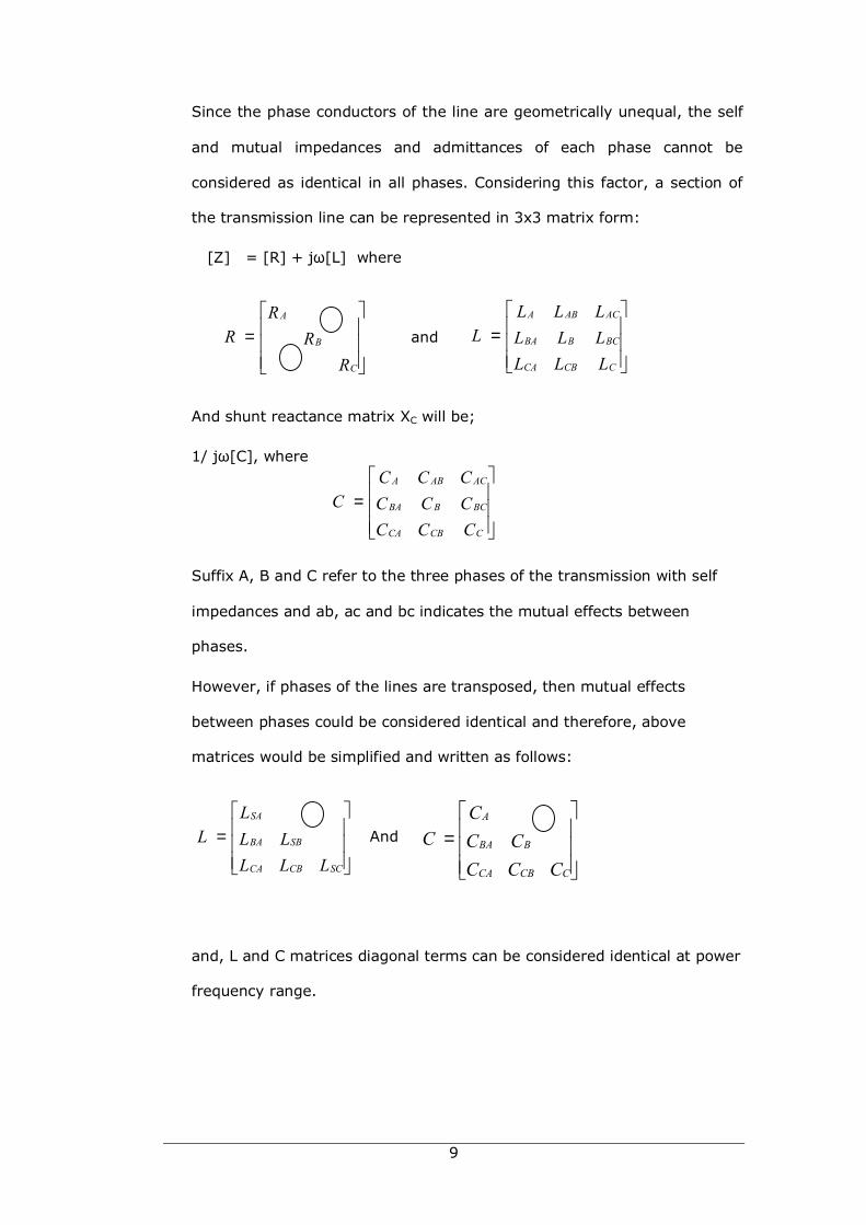
Since the phase conductors of the line are geometrically unequal, the self
and mutual impedances and admittances of each phase cannot be
considered as identical in all phases. Considering this factor, a section of
the transmission line can be represented in 3x3 matrix form:
[Z] = [R] + jω[L] where
and
And shunt reactance matrix XC will be;
1/ jω[C], where
Suffix A, B and C refer to the three phases of the transmission with self
impedances and ab, ac and bc indicates the mutual effects between
phases.
However, if phases of the lines are transposed, then mutual effects
between phases could be considered identical and therefore, above
matrices would be simplified and written as follows:
And
and, L and C matrices diagonal terms can be considered identical at power
frequency range.
=
LLLLLLLLL
L
CCBCA
BCBBA
ACABA
=
CCCCCCCCC
C
CCBCA
BCBBA
ACABA
=
RR
RR
C
B
A
=
LLLLL
LL
SCCBCA
SBBA
SA
=
CCCCC
CC
CCBCA
BBA
A
10
2.2.2 Shunt capacitance
In the case of long high voltage transmission lines, shunt capacitive
currents can be considerably larger in comparison to fault current,
particularly in high resistance fault cases[14]. Most fault location
algorithms do not consider shunt capacitance and hence cannot be applied
in the case of long transmission lines to estimate the location of faults
accurately. However, if the lines are short, the shunt currents can be
neglected for the location of a fault[10].
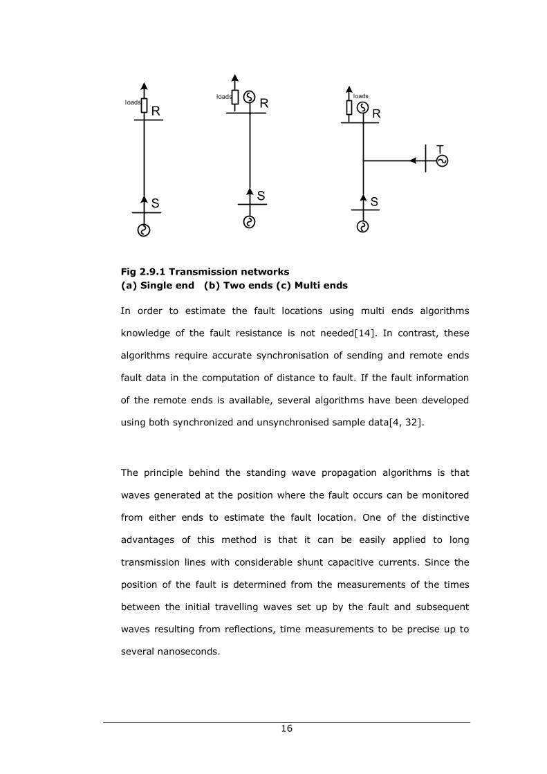
2.3 Transmission line configurations
Another important issue in developing a robust fault location algorithm is
that transmission lines have several configurations:
1. Transmission networks feed from one end.
2. Transmission networks feed from two ends
3. Transmission networks with multi ends
During a fault, in a single supply transmission network, fault current is fed
only from one end and hence remote end fault current measurements are
not required to estimate the location of fault in such networks. In this
case, remote end signal measurements and synchronisation problems are
not required for the estimation of a fault location. However, the accurate
estimation of remote source impedance is required in most cases and
hence it is difficult to estimate the location of the fault correctly.
In the case of two ends transmission network, signals from both ends can
be used for the estimation of a fault distance, and hence the fault
resistance which is one of the unknowns can be eliminated from the
network fault equation. The successful achievement of synchronising of
11
fault signals from remote end with fault locator end signals can be
obtained using GPS data communication methods and, are presented later
in this chapter. The fault location methods for transmission networks
with multi ends are not considered in this research.
2.4 Transmission line faults
In order to develop a robust and accurate fault location algorithm, fault
currents voltages data are required during a part of or entire fault
duration, which is highly, dependent on the fault network and its
configuration. Since the fault currents are directly related to the type of
fault, it is important to study the types of faults which can occur in the
transmission network.
Depending on the number of phases involved with the fault and how the
faulty lines are connected to the earth, five types of faults can be
identified as follows:
1. Single line to earth fault ( 1PG )
2. Double line fault (PP)
3. Double lines to earth fault ( PPG)
4. Three phase fault (PPP)
5. Three phase to earth fault ( PPPG)
In general it is required to know the type of fault by analysing the
recorded fault signals prior to estimating the fault location. Using ANN
algorithm developed by other authors it is possible to estimate the type of
fault accurately, analysing the fault currents and voltages signals[15].
12
The fault currents in a faulted transmission network are also highly
dependent on the fault impedance to the ground. For example, if the fault
impedance is high, fault currents will be very small and this affects the
accuracy of fault location. In this case, the direct impedance measurement
methods are not suitable for estimation of fault distance accurately[8]. In
certain fault cases, fault resistance changes with time during the fault[16,
17]. In such situations, most existing fault location algorithms are unable
to estimate the location of fault accurately. This is because these
algorithms are developed considering faulty signals during most of the
fault period and assumes constant fault impedance.
2.5 Fault duration
Most transmission line faults are caused by lightning strikes on
transmission towers and 90% of these are short duration temporary
faults. When a fault occurs in a transmission network, it will be first
detected by the protective relays which quickly command signals to
relevant circuit breakers to isolate the faulty part of the network. During
severe faults, this duration could be less then 2 to 3 cycles[2].
During this period, the fault locator must collect and store fault data
samples of voltages and currents of faulty line. This clearly shows that in
most fault cases fault locators will be able to record only 2 to 3 cycles of
data.
2.6: Fault location and resistance
When considering a single line transmission network where power is
supplied from one end, fault current is directly related to the location of
the fault from the supply end. If the supply end phaser values of the fault
13
network are measured during the fault, the location of the fault can be
computed quite easily without considering in feed from other ends.
Two ends single transmission line fault has in feed fault currents from
receiving ends hence two ends network equations need to be solved in
order to estimate the location of the fault. In this case, the total current
through the fault is the summation of sending and receiving ends fault
currents[18, 19].
In the case of parallel lines or multi ends transmission networks, fault
currents associated with the network configuration must be taken into
account in computing the fault location.
2.7 Data communication
Single end fault locators require only current and voltage data from the
local end of the transmission line, where data signals are directly available
to the locator[1, 7]. However, single ended fault location algorithms do
not estimate the location fault accurately, and neither, can these could be
used in complicated transmission networks.
With two ends fault location algorithms the unknown fault resistance can
be eliminated from the fault equation, hence leading to more accurate
fault location. But this necessitates the transfer of data from the remote
end to local end, so that fault location can be estimated. More importantly,
local and remote ends fault data samples must have very accurate time
tags so that sample values can be related and passed to the fault location
algorithm.
14
2.8 Fault location estimation
Computation of distance to fault in a transmission line involves three basic
steps namely fault detection, data communication and fault location. When
a fault is detected, recording of voltages and currents of the fault network
must be initiated in order to compute the location of the fault. In fault
detection, the fault locator is required to identify the fault type and hence
derive the fault impedance matrix before fault location is estimated[20].
In two-end algorithms data communication is required between local and
remote end with absolute synchronism.
2.9 Existing fault location methods
Due to the importance of transmission line fault detection, great efforts
have been undertaken by many research groups to obtain robust and
more accurate fault locations estimates over the years. The existing fault
location techniques can be grouped into several categories[9, 21-29]:
• Using fundamental components of the voltage and current signals
of the faulted network.
• Using time domain analysis on the differential equation based
model
• Using Travelling wave based method to solve faulted network
equations
• Using the high frequency transients generated by the faults
The most commonly based method in the past has been the phaser based
approach considering fundamental components of the fault signals.
On a simple transmission line network, the fault location and the
monitored voltages and currents are linked together through Ohm’s law.
Various signal processing techniques such as the Fourier transform and
15
Kalman filtering have been implemented in order to extract the
fundamental phasors of the monitored voltages and currents[2, 30]. Then
fault location can be estimated using the fault network equation,
substituting the computed phasors voltages and currents. Since the
faulted current and voltages are not purely sinusoidal, the accuracy of
fault location estimations using this method is limited[31]. This method
also fails in the case of reactive power compensated transmission
networks where compensation is achieved by highly nonlinear devices
such as series capacitors and more advanced thyristor based FACTs
controllers.
Increased accuracy has been achieved in other approaches. In particular
the direct use of synchronously sampled instantaneous fault data has
shown that fault location can be accurately estimated with definite
improvements in performance.
When considering classification of algorithms, accuracy of fault location
found to be further dependent on the following network configurations:
• One-end, transmission network
• Two-ends transmission network
• Multi-ends transmission network
The one end algorithm is the simplest and dispenses with synchronised
data communications with the other ends of the transmission network.
However, accuracy of such algorithm is adversely affected by the fault
resistance, series compensation devices and fault in feed from remote
ends.
16
Fig 2.9.1 Transmission networks (a) Single end (b) Two ends (c) Multi ends
In order to estimate the fault locations using multi ends algorithms
knowledge of the fault resistance is not needed[14]. In contrast, these
algorithms require accurate synchronisation of sending and remote ends
fault data in the computation of distance to fault. If the fault information
of the remote ends is available, several algorithms have been developed
using both synchronized and unsynchronised sample data[4, 32].
The principle behind the standing wave propagation algorithms is that
waves generated at the position where the fault occurs can be monitored
from either ends to estimate the fault location. One of the distinctive
advantages of this method is that it can be easily applied to long
transmission lines with considerable shunt capacitive currents. Since the
position of the fault is determined from the measurements of the times
between the initial travelling waves set up by the fault and subsequent
waves resulting from reflections, time measurements to be precise up to
several nanoseconds.
S
Rloads
loads
S
R
S
R
T
loads

17
The algorithms based on high frequency transients generated by the faults
can be found in number of papers published by other authors[33]. In
these methods, travelling waves generated by the fault is used in locating
the transmission line faults. One advantage of such methods is that fault
location accuracy is improved and insensitivity to series compensation
devices[34]. However, these methods require accurate measuring devices
to collect fault data during the fault. Another critical short coming of this
method is that it fails to produce reliable results for a fault that occurs
beyond the other end of the line.
2.10 Problems with existing methods
The most common problem with existing fault location algorithms is that
fault location is estimated considering the apparent reactance to the fault
from the fault locator. In most cases, the apparent reactance is computed
using the ratio of fundamental voltage and current phasors seen from the
fault locator. Firstly, the fault signals are filtered typically with suitable
Kalman filters on the raw fault signals to extract and then estimate the
power frequency voltages and currents. The raw fault signals are recorded
in either protection relays as the secondary functions of distance relays, or
measured by measuring devices incorporated with fault locators[35].
2.10.1 Apparent reactance
In series compensated line there will be a discontinuity in apparent
transmission line reactance as seen from the fault locator, due to the
operation of protection devices in the series capacitor. Even in basic series
compensation configuration, where spark gaps (creating varying
resistance) are incorporated, during heavy faults, operation of the Metal
Oxide Varistor (introducing a varying and non-linear resistance) and the
18
bypass circuit breaker virtually short circuit the series compensation[36].
Therefore it is extremely difficult to accurately estimate the fault signal
system frequency components. In the past there have been many
research papers published with several ways to estimate approximate
power frequency phasors in the case of series compensated lines, but the
results are marginal and cannot be implemented practically[1, 2].
Moreover, the modern series compensated devices are far more
complicated in which power flow in the transmission line is controlled by
changing the firing angle in order to damp subsynchronous resonance. In
such cases, it is almost impossible to reconstruct power frequency fault
signals using the fault signals recorded during fault duration of typically
less than 2 cycles[35].
2.10.2 Fault signal monitoring
Data for the fault locator is obtained either locally and/or at remote site
depends on the position of the fault locator and the system configuration.
Whatever the case, fault signals are sampled at a required frequency and
collected digitised signals are passed to the fault location equipment to
estimate the location. In most cases where direct or indirect impedance
measurement based algorithms are used, the sampling rate of 1 to 5 KHz
of data measurements is sufficient to obtain the required accuracy[35].
When the remote end fault signals are required for the estimation of fault
location, the synchronisation of signals can be achieved in several ways:
• Zero crossing detection
• Rotation of samples (for phasors)
• Using accurate time reference
19
The first two methods are used in most of the conventional fault location
methods of the past and synchronisation accuracy is less effective in
implementation of such algorithms. However, it was observed that fault
location methods using time domain approaches require more accurate
fault signal measurements and synchronisation. In this case, sampling
frequency as high as 100 KHz may be required with higher accuracy of
synchronising, which can be implemented using GPS based recording with
accurate time references[6, 18, 19, 31, 37].
2.11 Proposed fault location algorithms
2.11.1 Phasor based approach
We have developed first fault location algorithm for series compensated
line with just MOV operation by filtering and constructing approximate
power frequency signals to dynamically estimate the fault location using
fault data recorded from both ends of the two port transmission network.
This method is an improvement to fault location algorithm suggested by
author Saha [2, 38].
In this method, the algorithm is developed in phase coordinates and the
series capacitor and its protection device MOV are modelled in phase
equivalent in order to estimate the location fault solving system fault
equation. Since V-I characteristics of the series compensation is known,
the equivalent series resistance capacitor combination can be found and
resistive and reactive voltage drops can be computed depending on the
fault case. It is observed that values of both the resistance and the
reactance depend on amplitude of the fault current flowing through the
device. Therefore the series compensation is modelled in a testing
environment and hence the voltage drops with different amplitudes of
20
fault currents are recorded before the fault location algorithm is
implemented. For this purpose Saha[2] paper presented two methods:
• Using the analytical method where a sine wave of current is
injected to the series device to calculate the fundamental frequency
of the voltage drop to derive the resulting impedance of series
device.
• The simulation technique places the device in a natural system
configuration and estimates the fundamental frequency phasors of
both current and the voltage drop and then the resulting
impedance.
More details of phasor based fault location algorithm development with
modelling and testing in MATLAB environment are discussed in Chapter 3
[1].
2.11.2 Time domain approach
There are two ways of applying time domain approach in the location of
faults in transmission lines:
• Using direct transient fault signal waves
• Travelling wave method using reflected waves
It was observed that using direct transient fault signals, the fault location
can be estimated very accurately provided fault data is available to the fault
locator to the accuracy stated in the previous section[10, 16, 39]. There are
several advantages in using the time domain approach compared to other
methods to develop new fault location methods:
21
• Higher accuracy of fault location with a variety of operations and
fault conditions
• Can be used in both transposed and untransposed transmission lines
with different system configurations
• Fault resistance variations during the fault, does not affect the
accuracy of fault location
• Nonlinearity caused by the FACTs devices can be modelled in the
algorithms without significantly affecting the accuracy of fault
location
The modelling of FACTs series compensator and development of new fault
location algorithms using time domain signals are presented in chapter 6
and 7[18, 40].
2.12 Implementation issues with regard to new algorithms
In this research, two implementation approaches are investigated and these
strategies are briefly described as follows:
2.12.1 Phasor based approach
One of the major issues in the application of phasor based fault location
algorithm is estimating phasors from the recorded voltages and currents
during the fault. In most fault cases in high voltage transmission lines fault
recording time is less than one cycle of fundamental frequency causing
difficulties in estimating phasor values of faulted signals. Some authors
22
have presented methods such as, curve fitting, correlations and
nonrecursive filters with variable data windows, in order to overcome this
problems.[2, 41] At the same time harmonics which are always presented
in the faulted signals must be suppressed as much as possible. The most
commonly used method of solving this problem is by incorporating Kalman
filtration. Therefore, additional components either in hardware or software
are required before implementing the fault location algorithm.
Another problem is that most fault location algorithms are required
knowledge of the type of fault, prior to estimating fault distance. An
external device or algorithm is required to identify the type of fault as
stated in section 2.4. This information is passed to fault locator with the
fault data to estimate the location of fault.
2.12.2 Time domain approach
As this is already discussed briefly in the previous section, it is important to
discuss one of the major problems associated with estimation of fault
distance using time domain signals, which is the accuracy of signal
measurements and synchronisation. The accuracy of data measurement
with higher sampling rate can be achieved easily using higher class
capacitor coupling voltage transformer (CCVT) with current transformers
with reasonably matched A/D converters[2].
But the difficulty is that measured fault data must be time tagged at regular
intervals with absolute time reference for later synchronisation of local and
remote data. If the signals are sampled at 100 KHz, the time difference
between two consecutive sample measurements is 0.01 ms. Even though
this seems impossible to achieve practically, new modern GPS based
devices are emerging in to the market with much more accurate timing.
23
One such example is Hewlett Packard (HP) 59551A GPS measurements
synchronisation unit designed specially for power system operations with
precision timing based on advanced GPS technology[42]. HP claimed that
HP 59551A together with HP’s SmartClock technology can provide the
accuracy of timing up to 110 nanoseconds with 95% probability[42].
2.12.3 Further improvements
The new fault location methods presented in this research work still needs
further improvement to implement in a real power transmission
environment especially with FACTs devices and different transmission
configurations. Since the phasor based fault location method is not the
main focus of this research and cannot be applied for FACTs series
compensation, improvements suggested in this section refers to the time
domain approach methods[18]. These are as follows:
• Algorithm development for long transmission lines are very basic and
has not been tested for different system configurations. No statistical
testing has been conducted with varying shunt capacitance, series
compensation or with different type of FACTs devices with
dynamically changing series capacitance.
• With regards to the parallel transmission line, the only theory that
has been established and a simple test case has been built is for the
initial testing of the new algorithm.
• The algorithm has not been tested for multi end transmission
networks. In this case the new selection algorithm is required for
24
the general location of the fault and type of fault as the input to
algorithms presented in this research.
2.13 Summary
In this chapter reviews a mathematical modelling of the transmission
networks and the existing concepts in relation to the developing of a fault
location algorithm. The two concepts of developing algorithms used in this
thesis are presented considering the practical issues of implementing on
different network configurations. At the end of this chapter methods of
further improving the fault location algorithm are presented.
25
Chapter 3.0
Development of a new algorithm
for Fault location estimation
3.1 Introduction
In the previous chapter past and newly developed fault location concepts and
associated design and implementation issues with respect to each concept
were discussed. In this chapter the very first fault location algorithm
developed in these research works is discussed[1].
This method uses the phasor based approach and the algorithm can be
applied to a series of compensated transmission lines for estimation of fault
location. The two ends series compensated transmission line model has been
built using MATLAB Power System Block sets and fault data from the
simulation read from the fault location algorithm to estimate the location of
the fault[6].
Performance evaluation of the algorithm is discussed at the end of this
chapter considering the number of practical implementation issues and
limitations, with regards to different transmission line configurations.
3.2 Supply system
Single phase alternative supply source can be expressed in a mathematical form with respect to time:
V(t) = VM Sin( ωt + Q ) (3.2.1)
26
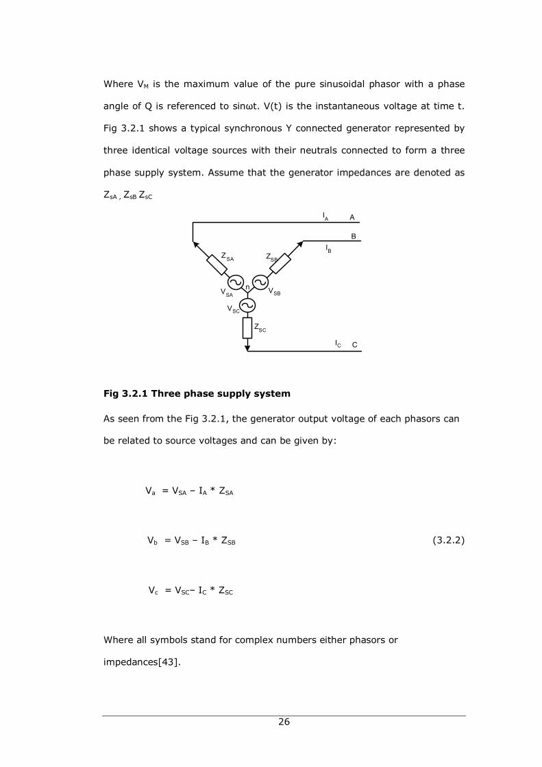
Where VM is the maximum value of the pure sinusoidal phasor with a phase
angle of Q is referenced to sinωt. V(t) is the instantaneous voltage at time t.
Fig 3.2.1 shows a typical synchronous Y connected generator represented by
three identical voltage sources with their neutrals connected to form a three
phase supply system. Assume that the generator impedances are denoted as
ZsA , ZsB ZsC
Fig 3.2.1 Three phase supply system
As seen from the Fig 3.2.1, the generator output voltage of each phasors can
be related to source voltages and can be given by:
Va = VSA – IA * ZSA
Vb = VSB – IB * ZSB (3.2.2)
Vc = VSC– IC * ZSC
Where all symbols stand for complex numbers either phasors or
impedances[43].
n
ZSA ZSB
ZSC
A
B
C
VSAVSB
VSC
IA
IB
IC
27
Considering the mutual coupling among the three phases of the generator,
the equation (3.2.2) can be written in matrix form as follows:
(3.2.3)
In this case it is assumed that the mutual couplings between phases are
identical and phase lines are also identical[2].
3.3 Transmission line
The transmission line also can be expressed similar to the supply source
impedance matrix, neglecting the line shunt capacitance. If the transmission
line is short and completely transposed, these assumptions can be considered
valid for fault location algorithm development[43].
3.4 Fault resistance
Transmission line faults and faults currents during faults are discussed broadly
in the previous chapter. However, it is necessary to study mathematical
modelling of faults which represents a broad spectrum of transmission line
faults. In order to handle symmetrical and unsymmetrical faults a model can
be developed as shown in Fig 3.4.1[2, 44].
Fig 3.4.1 General fault model
Ss Sm Sm AA SA
Sm Ss Sm BB SB
Sm Sm Ss CC SC
V V Z Z Z IV V Z Z Z IV V Z Z Z I
= −
Rab Rbc
Rac
Ra Rb Rc
Va
Vb
Vc
IaIb
Ic
a
b
c
28
In this model, Rg represents the ground fault resistance and Rn is the
apparent resistance between phases during the faults. Controlling switches a,
b and c in this model can create phase-to-phase faults, phase-to-ground
faults, or a combination of phase-to-phase and ground faults[2]. The
conductance matrix G can be derived considering the above fault model as
follows:
(3.4.1)
where (3.4.2)
and IF and VF are fault current and fault voltage.
If the apparent fault resistance from phase to fault is Rf, another matrix
relationship can be derived considering different types of faults:
(3.4.3)
where matrix can be configured depends on single phase or multi
phase faults. For an example, in the case of phase a-b-g and a-b faults,
takes the form:
(3.4.4)
and respectively.
The rf is the total aggregated fault resistance referred to the faulty phases[2].
1 1 1 1 1
1 1 1 1 1
1 1 1 1 1
a ab ac ab ac
ab b ab bc bc
ac bc c bc ac
r r r r r
r r r r r
r r r r r
+ + − − − + + − − − + +
[ ] [ ] [ ]f fG VI =
[ ] [ ]1F
f
G Kr
=
[ ]FK[ ]FK
2 1 01 2 0
0 0 0
− −
1 1 01 1 0
0 0 0
− −
29
3.5 Measurements of fault data
Fault signal measuring accuracy and the available recording duration are
dominant factors when considering the measurement of fault data in order to
estimate the location of the fault. Since the fault signal contains harmonics
and dc component it is difficult to accurately measure the fault signal
amplitude and phase. Therefore power frequency voltages and current
measurements using ordinary VT’s and CT’s may not be sufficient to measure
fault signals. In most fault cases the fault recoding time available is limited as
the relays initiate the tripping signal to clear the fault in short time.
Therefore the fault data available for the recorder may not be sufficient
enough to estimate the phasors of fault signals.
When the digital fault recorders are used for monitoring and recording of fault
signals, a minimum of 1 KHz sampling of signals are required to reconstruct
the phaser value of signals[9]. These issues are discussed in a number of
papers in which Kalman filtration, curve fitting methods, correlation and non
recursive filters with varying data windows have been used for estimation of
power frequency voltage and current phasors.[35]
In the case of one end fault location methods, fault signals are measured only
from one end and therefore measurements of voltages and currents act as a
reference to each other. But the accuracy of the estimation of fault location
highly depends on the other factors such as resistance changing during the
fault, and the inability to estimate remote source impedance accurately.
These issues can be almost solved with the signals measured from the remote
end and transmitting to local end for the estimation of fault distance.
However, most two ends fault location algorithms discussed by many authors
30
suggest that accuracy of the signal sample synchronisation from the remote
end is dominant in the implementation of such algorithms, which will be
discussed in chapter 7 in more details[34, 41].
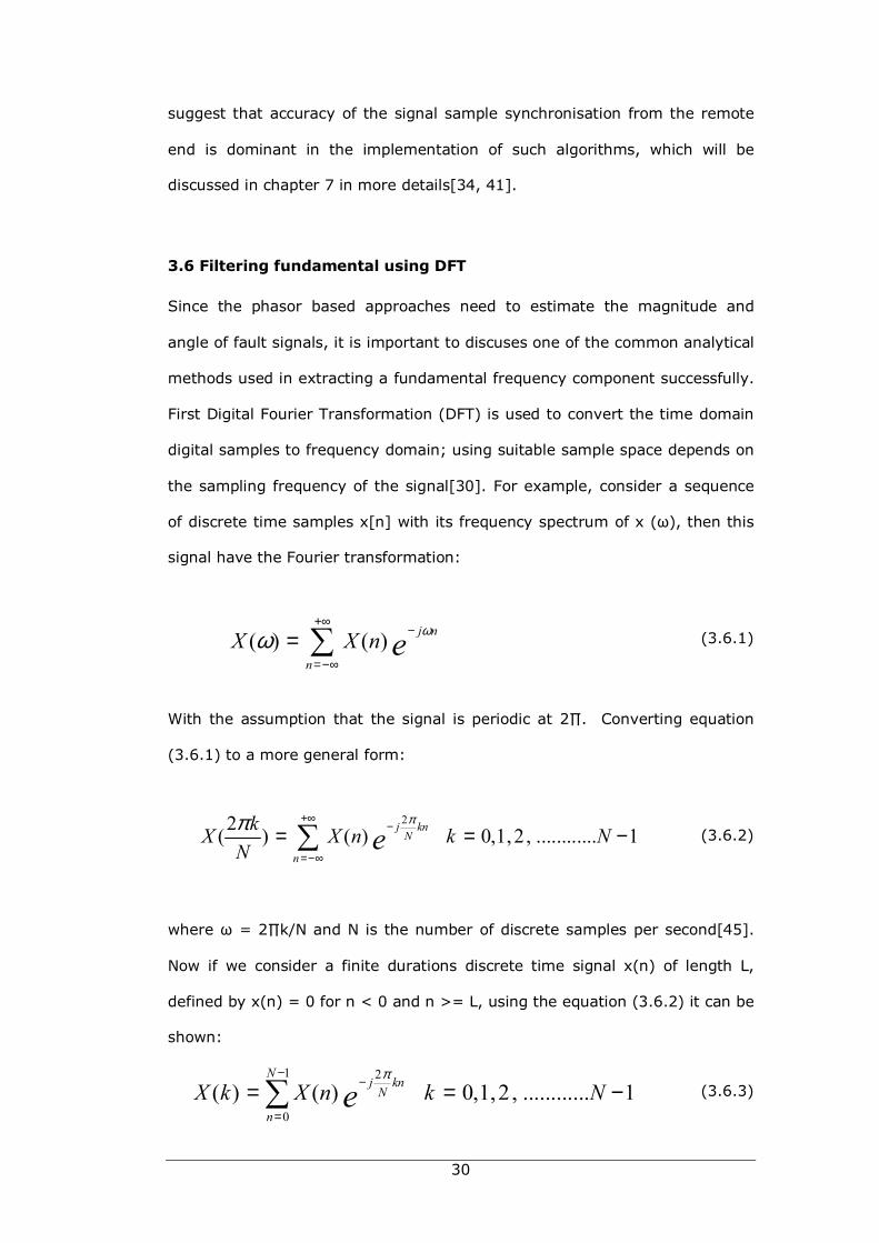
3.6 Filtering fundamental using DFT
Since the phasor based approaches need to estimate the magnitude and
angle of fault signals, it is important to discuses one of the common analytical
methods used in extracting a fundamental frequency component successfully.
First Digital Fourier Transformation (DFT) is used to convert the time domain
digital samples to frequency domain; using suitable sample space depends on
the sampling frequency of the signal[30]. For example, consider a sequence
of discrete time samples x[n] with its frequency spectrum of x (ω), then this
signal have the Fourier transformation:
(3.6.1)
With the assumption that the signal is periodic at 2∏. Converting equation
(3.6.1) to a more general form:
(3.6.2)
where ω = 2∏k/N and N is the number of discrete samples per second[45].
Now if we consider a finite durations discrete time signal x(n) of length L,
defined by x(n) = 0 for n < 0 and n >= L, using the equation (3.6.2) it can be
shown:
(3.6.3)
( ) ( ) j n
nX X n e ωω
+∞−
=−∞
= ∑
22( ) ( ) 0,1,2, ............ 1j knN
n
kX X n k NN e
ππ +∞−
=−∞
= = −∑
1 2
0
( ) ( ) 0,1,2 , ............ 1N
j knN
n
X k X n k Neπ−
−
=
= = −∑
31
where the upper index in the summation is increased from L-1 to N-1 for
convenience. The relationship in equation (3.6.3) shows that a given
sequence of signals X[n] in the space of L <- N can be transformed in
sequence of samples in frequency domain X[k] of length N. This
transformation is called the Discrete Fourier Transformation. (DFT)
3.7 Series compensated lines
Basic modelling of the standard transition line discussed in the previous
chapter can be used for developing a fault location algorithm. However, in the
recent past new FACTS technology has been used in many transmission
networks to control the power transfer in the line, with many other
advantages such as higher power transferability, damping of oscillations and
improvements to stability etc[12]. The details of transmission line
configuration and insuring FACTS devices are described in chapter 5. The next
section describes the detail modelling of series line compensation which is a
cornerstone of FACTS technology.
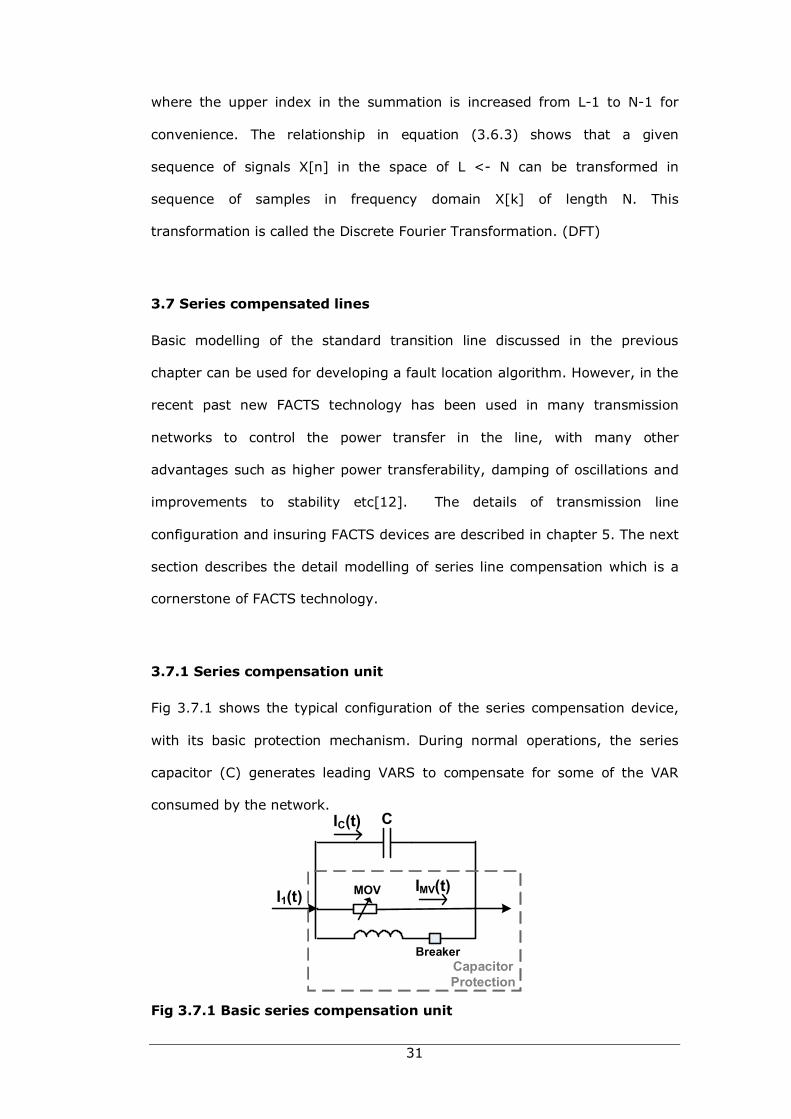
3.7.1 Series compensation unit
Fig 3.7.1 shows the typical configuration of the series compensation device,
with its basic protection mechanism. During normal operations, the series
capacitor (C) generates leading VARS to compensate for some of the VAR
consumed by the network.
Fig 3.7.1 Basic series compensation unit
IC(t)
MOV
C
Breaker
IMV(t)I1(t)
Capacitor Protection
32
The Metal Oxide Varistor (MOV) is the main protection device, which operates
when an over voltage is detected across the capacitor. With a short circuit on
the line, the capacitor is subjected to an extremely high voltage, which is
controlled by the conduction of MOV. The voltage protection level of MOV
(1.5pu to 2.0pu) is determined with reference to the capacitor voltage drop
with rated current flowing through it[46]. The VI–characteristics of the MOV
can be approximated by a nonlinear equation:
(3.7.1)
where p and VREF are coordinates of the knee point of MOV and q is an
exponent of the MOV characteristics[11, 47].
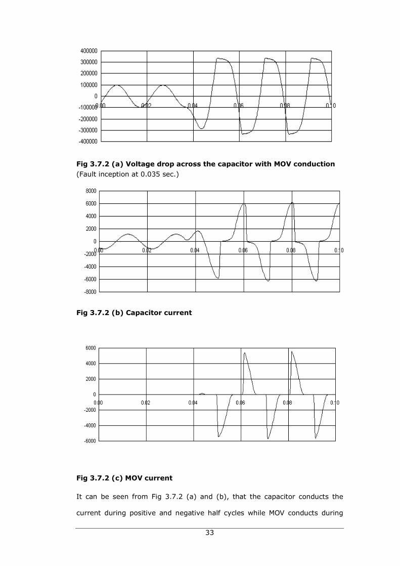
3.7.2 Series compensation voltage drop
Under normal load conditions or with low fault currents, neither the air gap
nor the MOV conducts any currents. Therefore the SC voltage drop is caused
by the capacitor reactance. Under very high fault current, where the voltage
drop across the capacitor exceeds its protection level, the majority of the
through current is passed through the MOV and the air gap[37].
In between those two conditions, fault current is divided considerably
between the capacitor and MOV. Fig 3.7.2 illustrates voltage and currents
across the series compensation unit. When the through current is higher the
drop across the capacitor becomes more rectangular due to the voltage
protection level as shown in Fig 3.7.2 (a).
=VREFVpi
q
*
33
Fig 3.7.2 (a) Voltage drop across the capacitor with MOV conduction (Fault inception at 0.035 sec.)
Fig 3.7.2 (b) Capacitor current
Fig 3.7.2 (c) MOV current
It can be seen from Fig 3.7.2 (a) and (b), that the capacitor conducts the
current during positive and negative half cycles while MOV conducts during
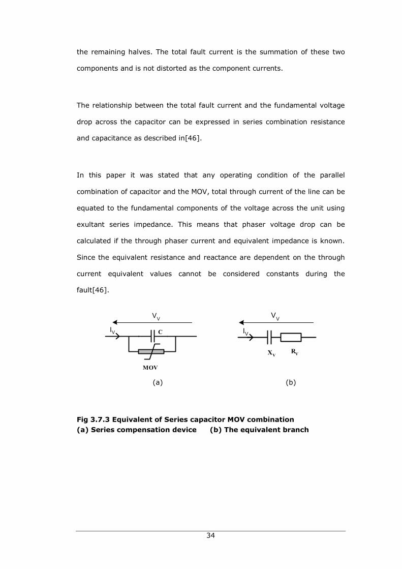
34
the remaining halves. The total fault current is the summation of these two
components and is not distorted as the component currents.
The relationship between the total fault current and the fundamental voltage
drop across the capacitor can be expressed in series combination resistance
and capacitance as described in[46].
In this paper it was stated that any operating condition of the parallel
combination of capacitor and the MOV, total through current of the line can be
equated to the fundamental components of the voltage across the unit using
exultant series impedance. This means that phaser voltage drop can be
calculated if the through phaser current and equivalent impedance is known.
Since the equivalent resistance and reactance are dependent on the through
current equivalent values cannot be considered constants during the
fault[46].
(a) (b)
Fig 3.7.3 Equivalent of Series capacitor MOV combination (a) Series compensation device (b) The equivalent branch
IV
MOV
C
VV
IV
XV
VV
RV
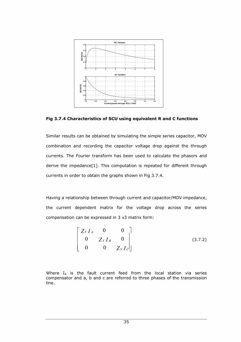
35
Fig 3.7.4 Characteristics of SCU using equivalent R and C functions
Similar results can be obtained by simulating the simple series capacitor, MOV
combination and recording the capacitor voltage drop against the through
currents. The Fourier transform has been used to calculate the phasors and
derive the impedance[1]. This computation is repeated for different through
currents in order to obtain the graphs shown in Fig 3.7.4.
Having a relationship between through current and capacitor/MOV impedance,
the current dependent matrix for the voltage drop across the series
compensation can be expressed in 3 x3 matrix form:
(3.7.2)
Where IA is the fault current feed from the local station via series compensator and a, b and c are referred to three phases of the transmission line.
1 2 3 4 5 6 7 80
0.1
0.2
0.3
0.4
(RC
/XC
O)
RC Variation
1.0 2.0 3.0 4.0 5.0 6.0 7.0 8.00
0.2
0.4
0.6
0.8
1
Current passes through SCU ( I /Iref)
(XC
/XC
O)
XC Variation
0 00 00 0
V A
V B
V C
Z IZ I
Z I
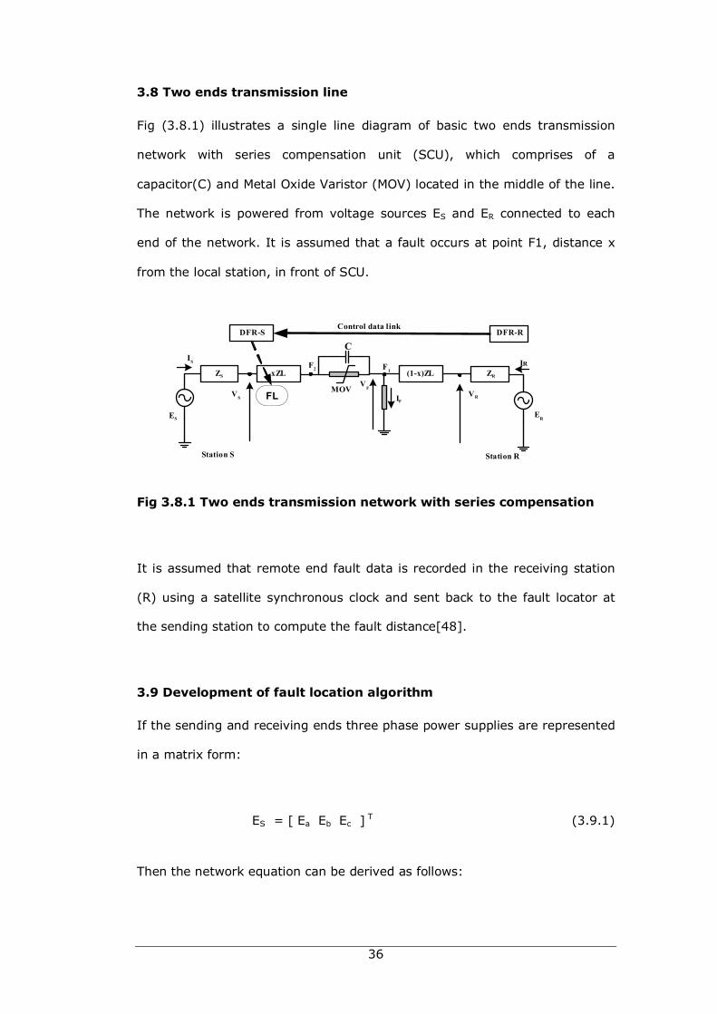
36
3.8 Two ends transmission line
Fig (3.8.1) illustrates a single line diagram of basic two ends transmission
network with series compensation unit (SCU), which comprises of a
capacitor(C) and Metal Oxide Varistor (MOV) located in the middle of the line.
The network is powered from voltage sources ES and ER connected to each
end of the network. It is assumed that a fault occurs at point F1, distance x
from the local station, in front of SCU.
Fig 3.8.1 Two ends transmission network with series compensation
It is assumed that remote end fault data is recorded in the receiving station
(R) using a satellite synchronous clock and sent back to the fault locator at
the sending station to compute the fault distance[48].
3.9 Development of fault location algorithm
If the sending and receiving ends three phase power supplies are represented
in a matrix form:
ES = [ Ea Eb Ec ] T (3.9.1)
Then the network equation can be derived as follows:
ES
(1-x)ZL
MOV
C
VF
F2
IF
F1
Station RStation S
ZS xZL
IS
VS FL
ZR
ER
IR
VR
DFR-S DFR-RControl data link
37
ES – ER = (ZS + xZL+ ZV) ISS - ((1-x)ZL + ZR)IRR (3.9.2)
where ZL and ZV are transmission line and series compensator impedances
respectively. In this case, ZV is pre computed using both sending and
receiving ends fault currents over a range of values with the identical series
compensation as explained in section 3.7.2 and available for the fault location
algorithm prior to the estimation of the fault distance.
The change in supply sources ES and ER are very small before and after the
occurrence of the fault and hence ES – ER can be computed using pre fault
network signals and applied to the fault equation (3.9.2).
3.9.1 Fault location algorithm with remote end signals
If fault signal measurements are available from both ends of the line fault
distance x can be calculate solving equation (3.9.2). If the fault is on the
sending side of the line after the series compensation, equation (3.9.2) can be
rewritten as:
ZL[IS +IR] x = ∆E + (ZL + ZR)IR - (ZS + ZV)IS (3.9.3)
where [ZV IA] can be estimated as described in section 3.7.2 in relation to
fault current through the series compensator.
Similarly, if the fault is before the series compensation, the receiving end fault
current could be used to estimate the location of the fault:
ZL[IS +IR] x = ∆E + (ZL + ZS)IS - (ZR + ZV)IR (3.9.4)
Through the fault resistance another equation can be written looking from the
sending end relating to faulted voltage:
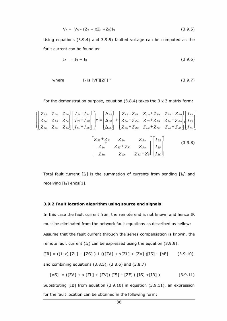
38
VF = VS - (ZS + xZL +ZV)IS (3.9.5)
Using equations (3.9.4) and 3.9.5) faulted voltage can be computed as the
fault current can be found as:
IF = IS + IR (3.9.6)
where IF is [VF][ZF]-1 (3.9.7)
For the demonstration purpose, equation (3.8.4) takes the 3 x 3 matrix form:
+
+ (3.9.8)
Total fault current [IF] is the summation of currents from sending [IS] and
receiving [IR] ends[1].
3.9.2 Fault location algorithm using source end signals
In this case the fault current from the remote end is not known and hence IR
must be eliminated from the network fault equations as described as bellow:
Assume that the fault current through the series compensation is known, the
remote fault current (IR) can be expressed using the equation (3.9.9):
[IR] = ((1-x) [ZL] + [ZS] )-1 (([ZA] + x[ZL] + [ZV] )[IS] – [∆E] (3.9.10)
and combining equations (3.8.5), (3.8.6) and (3.8.7)
[VS] = ([ZA] + x [ZL] + [ZV]) [IS] – [ZF] ( [IS] +[IR] ) (3.9.11)
Substituting [IB] from equation (3.9.10) in equation (3.9.11), an expression
for the fault location can be obtained in the following form:
LS Lm Lm SA RA EA LS RS Lm Rm Lm Rm RA
Lm LS Lm SB RB EB Lm Rm LS RS Lm Rm RB
Lm Lm LS SC RC EC Lm Rm Lm Rm LS RS RC
Z Z Z I I Z Z Z Z Z Z IxZ Z Z I I Z Z Z Z Z Z I
Z Z Z I I Z Z Z Z Z Z I
+ + + + ∆ + = + + + +∆ + + + +∆
SS V Sm Sm SA
Sm SS V Sm SB
Sm Sm SS V SC
Z Z Z Z IZ Z Z Z IZ Z Z Z I
+ + +
39
Ax2 + Bx +C –Rf = 0; (3.9.12)
where x and Rf are the two unknowns. Since the equation (3.9.12) involves
complex matrices, it can be divided to two ports using real and imaginary
components:
re[x] = ± f(re[Rf]) (3.9.13)
im[x] = ± f(im[Rf]) (3.9.14)
Finally, there are two unknowns (x and Rf) and two equations (3.9.13 and
3.9.14). Since equation (3.9.12) is quadratic, and it has two roots for x and
expanding each as above will produce several solutions to fault location and
resistance. However, incorrect solutions can be easily detected and easily
removed by ignoring negative values for x and Rf [14].
3.10 Testing of the algorithm
The algorithm with fault signal measurements obtained from both ends of the
series compensated transmission line has been tested with the two port
network shown in Fig 3.8.1 in the MATLAB 6.5 environment using MATLAB 6.5
Power System Blockset[49]. The basic Transmission line modelling using this
package is described in detail in chapter 4 section 7. In this section the
implementation of series compensation in testing this algorithm is discussed.
3.10.1 Series compensation
Fig 3.10.1 shows the single phase (phase A) implementation of a series
compensation model. The capacitor CS1 modelled with a series LRC
branch making R and L values to zeros and the capacitor value is set to
70% compensation of the line. Then the MOV1 represents the surge
arrester for the protection device of the capacitor. I-V characteristics of
this device are similar to metal oxide varistor used in the series
compensation networks. In this case only one exponential function is used
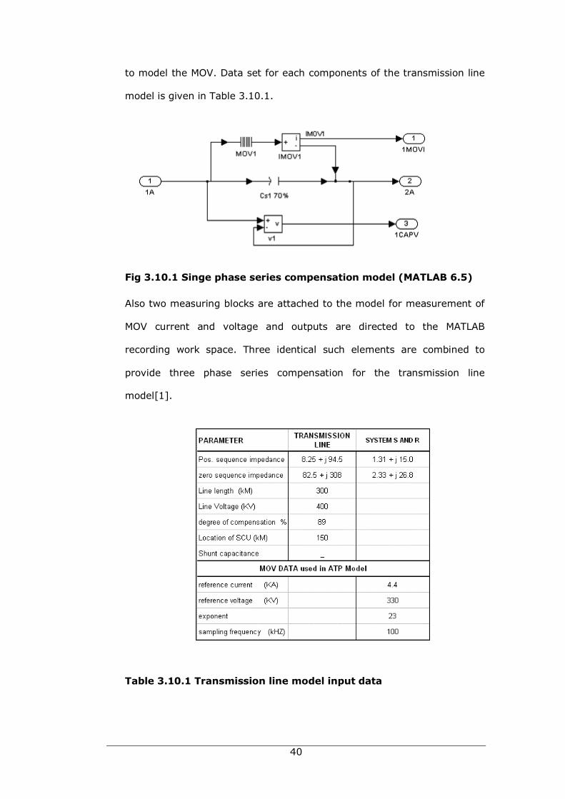
40
to model the MOV. Data set for each components of the transmission line
model is given in Table 3.10.1.
Fig 3.10.1 Singe phase series compensation model (MATLAB 6.5)
Also two measuring blocks are attached to the model for measurement of
MOV current and voltage and outputs are directed to the MATLAB
recording work space. Three identical such elements are combined to
provide three phase series compensation for the transmission line
model[1].
Table 3.10.1 Transmission line model input data
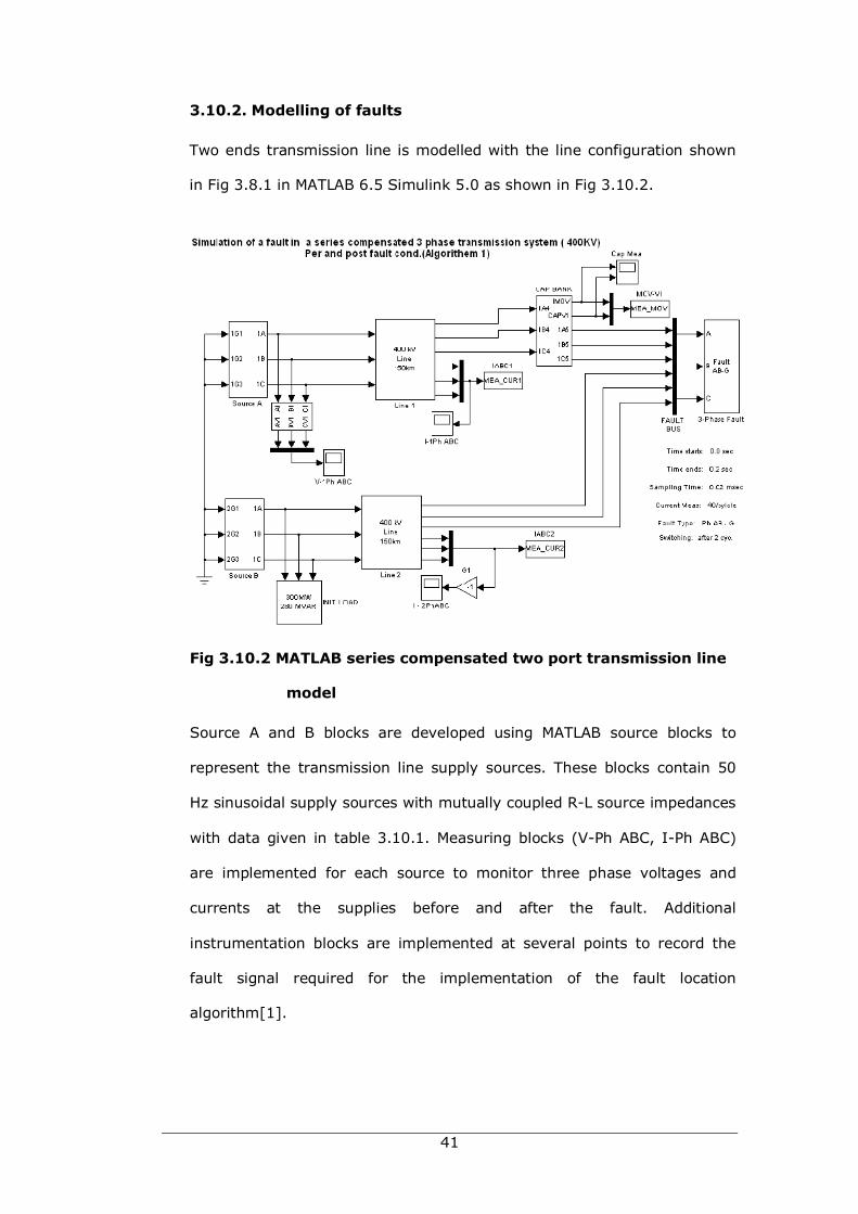
41
3.10.2. Modelling of faults
Two ends transmission line is modelled with the line configuration shown
in Fig 3.8.1 in MATLAB 6.5 Simulink 5.0 as shown in Fig 3.10.2.
Fig 3.10.2 MATLAB series compensated two port transmission line
model
Source A and B blocks are developed using MATLAB source blocks to
represent the transmission line supply sources. These blocks contain 50
Hz sinusoidal supply sources with mutually coupled R-L source impedances
with data given in table 3.10.1. Measuring blocks (V-Ph ABC, I-Ph ABC)
are implemented for each source to monitor three phase voltages and
currents at the supplies before and after the fault. Additional
instrumentation blocks are implemented at several points to record the
fault signal required for the implementation of the fault location
algorithm[1].
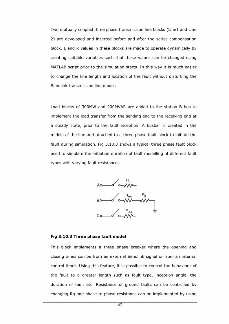
42
Two mutually coupled three phase transmission line blocks (Line1 and Line
2) are developed and inserted before and after the series compensation
block. L and R values in these blocks are made to operate dynamically by
creating suitable variables such that these values can be changed using
MATLAB script prior to the simulation starts. In this way it is much easier
to change the line length and location of the fault without disturbing the
Simulink transmission line model.
Load blocks of 300MW and 200MVAR are added to the station B bus to
implement the load transfer from the sending end to the receiving end at
a steady state, prior to the fault inception. A busbar is created in the
middle of the line and attached to a three phase fault block to initiate the
fault during simulation. Fig 3.10.3 shows a typical three phase fault block
used to simulate the initiation duration of fault modelling of different fault
types with varying fault resistances.
Fig 3.10.3 Three phase fault model
This block implements a three phase breaker where the opening and
closing times can be from an external Simulink signal or from an internal
control timer. Using this feature, it is possible to control the behaviour of
the fault to a greater length such as fault type, inception angle, the
duration of fault etc. Resistance of ground faults can be controlled by
changing Rg and phase to phase resistance can be implemented by using
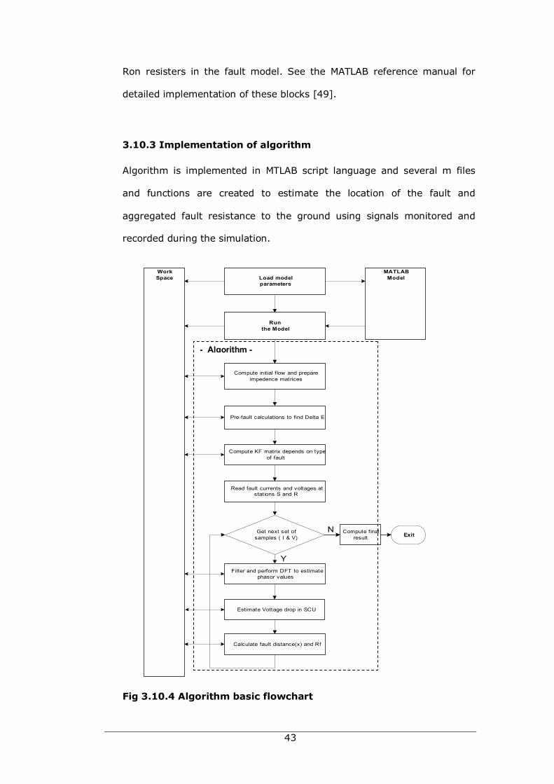
43
Ron resisters in the fault model. See the MATLAB reference manual for
detailed implementation of these blocks [49].
3.10.3 Implementation of algorithm
Algorithm is implemented in MTLAB script language and several m files
and functions are created to estimate the location of the fault and
aggregated fault resistance to the ground using signals monitored and
recorded during the simulation.
Fig 3.10.4 Algorithm basic flowchart
Load modelparameters
WorkSpace
MATLABModel
Runthe Model
Get next set ofsamples ( I & V)
Compute initial f low and prepareimpedence matrices
Pre-fault calculations to find Delta E
Compute KF matrix depends on typeof fault
Read fault currents and voltages atstations S and R
Filter and perform DFT to estimatephasor values
Estimate Vottage drop in SCU
Calculate fault distance(x) and Rf
Y
NExitCompute final
result
- Algorithm -
44
The fault location algorithm is written using MATLAB script language and
the basic flowchart of the function blocks are shown in Fig 3.10.4. At first,
data for the transmission line model is loaded to the MATLAB model shown
in Fig 3.10.2 using function “Load parameters”. This function takes the
arguments such as initial loading, fault location, fault resistance, type of
fault and level of compensation and compute parameter data required for
the model. Then it loads the model and sets the simulation to run it[1].
When the simulation is completed, fault signals saved on the MATLAB
workspace are used in the algorithm function blocks to compute the
location of the fault and fault resistance as follows[1]:
• Compute pre-fault load flow and line impedance matrices for the
algorithm
• Compute Es –ER arrays
• Compute KF matrix depends on the given fault type
• Read three phase fault signals from both ends of the line in to
MATLAB arrays
• Insert the BW filter and clean the signal arrays if ‘filter on’ is
selected
• Read first set of signal samples to fault location estimation loop
• Perform DFT and compute the phasor values of sending and
receiving voltages and currents
• Call the SC Blocks to estimate the voltage drop matrix of the
algorithm
• Estimate the location of fault and fault resistance
• Apply the selection algorithm to reject incorrect results
• Save the estimated correct values in dynamic result array
45
• Get the next set of fault signals and repeats the same processes
• Loop continues until reading all fault signal data
• At the end result arrays are further processed to compute the final
values for the fault location and fault resistance
3. 11 Evaluation of the algorithm
A detail case study of the implementation of this algorithm together with
simulation results and dynamic computation of fault distance and resistance
to the fault are given in chapter 11. For the statistical evaluation of this
algorithm, many different types of faults have been generated using the
MATLAB model described in sections 3.10.1 and 3.10.2 and the fault location
is estimated using the algorithm implemented in sections 3.10.3. In all fault
cases transmission line data is unchanged and different cases have been
generated with following variations:
Type of faults (single phase faults, three phase faults with and without ground
and phase to phase faults)
• Location of fault (0.2 pu, 0.5 pu and 0.75 pu)
• Fault resistance (1 and 10 ohm)
• Fault inception angle (00, 450 and 1350)
3.12 Comparison of results
At this stage, the fault location results estimated using this algorithm was
compared with the results given in Saha paper and details are in Chapter 8
[2]. It was observed that the new phasor based fault location algorithm is
considerably accurate compared to other algorithms and the conclusions are
briefly given below:
46
In general, the average fault location estimated error is significantly reduced
(from 0.4% to 1.2%) closer to the fault near to the middle of the line and
gradually increased closer to the ends (from 0.8% to 2%).
Higher fault location error is contributed due to the mismatching of data in
MATLAB transmission model and in algorithm.
Another issue that contributed to the error was due to a high level of
transients, presence in the MATLAB fault data and hence the phaser value
estimations are not accurate [50].
3.13 Practical issues
This section covers practical issues in implementing this algorithm in series
compensated transmission lines in order to estimate the location of faults with
higher accuracy.
3.13.1 Synchronisation error
One of the critical requirements of this newly developed algorithm is that
fault data measurement synchronisation is required from the remote end
to estimate the location of a fault. In general, remote fault data
measurements are carried out by the digital distance relays in modern
power systems with sampling of 1 KHz and can be readily available to the
local end of the line[35]. However, these signal samples are not accurately
time tagged to synchronise data with the local end. Therefore these
measurements can be used with external mathematical synchronisation to
estimate the location of the fault using this algorithm to the specified
accuracy given in table 8.12.1.
47
Nevertheless, precise data synchronisation of data from far ends can be
achieved with GPS based recording and synchronisation devices, which are
relatively low in cost, portable and make implementation much easier.
3.13.2 Prior knowledge of fault type
One of the requirements of using this fault location algorithm is the
knowledge of fault types. There are many works of research that have
been carried out addressing the identification of types of faults using
several approaches such as, fuzzy logic, neural networks and genetic
algorithms with very high success rates[38, 51, 52]. However, it was
observed that the accuracy in estimating the fault distance using this
method is badly affected if the fault type is not identified correctly.
3.13.3 Series compensated FACTs devices
The implementation and testing of this algorithm is strictly based on a
simplified series compensation device when considering only the main
protection of MOV operation. However, practically spark gaps are
incorporated in these devices to protect the MOV being overheated[14]. In
such cases operation of air gaps must be incorporated in the present
algorithm. Further, it will be almost impossible to estimate the location of
the fault, if the transmission lines are constructed with modern FACTs
series compensation devices.
This is because the thyristor controlled switching devices incorporated in
the FACTs makes it extremely difficult to estimate the series capacitor
voltage drop using the phasor equivalent impedance method.
48
3.13.4 Long transmission lines
The fault location algorithm is developed assuming that the line shunt
capacitance are negligible and hence the accuracy of estimations are valid
only for short transmission lines with minimal capacitive leakage currents.
It was observed that the inclusion of shunt capacitance in the line model
data, leads to another 1% drop in the accuracy of fault location. However,
in chapter 9, this thesis presents new fault locating methods that could be
successfully used in long transmission line with considerable capacitive
leakage currents.
3.14 Summary
This chapter develops a new algorithm for detecting faults on two ends
series compensated transmission lines using fault data collected from both
ends. First a model was developed for a simple series compensated unit
located in the middle of a transmission line to resolve the faulted network
equations to estimate the location of a fault. The new addition of Power
System Blockset for MATLAB is used for testing the new algorithm and the
results are evaluated and compared with a similar algorithm developed by
the author.
49
Chapter 4.0
Transmission lines Modelling
4.1 Introduction
The performance of a fault location algorithm can only be tested by studying
and analysing fault data observed during the fault. The most accurate
method of getting fault data is to use data recorded during actual system
faults, which is not always possible due to many practical reasons:
• Diversity of all types of fault data is impossible to obtain from actual
system faults.
• Inconsistency or sparse data.
• Precision of data – difficult to catch fine changes
• Synchronisation errors ( Fault data at terminals are not synchronised)
• Measuring equipment errors
Since power systems are large and interconnected to several geographic
areas to form a common network supplying power to millions of customers,
high voltage transmission lines are designed with very high reliability and
security[12]. Therefore, historical fault data available for fault location
detection is very much limited. In the recent past, protection relays installed
in transmission lines consisted of microprocessor based devices capable of
recording fault data in pre and past time periods during a fault. In most cases
50
however, the sampling rate of these recordings was not sufficient for testing
accurate fault location algorithms[10]. In addition, signal recordings at
multiple ends of the transmission lines are not synchronised nor have
accurate time tags for external synchronisations, making it difficult to use in
two ends fault location algorithms[18].
In general, fault location algorithms are required to test all types of faults and
the actual fault data obtained from real power systems do not have this
diversity.
The other alternative is to make a scaled down prototype of the faulted
network. But this method is costly and it is far more complex to design an
accurate transmission network model that will behave like the real power
network. Besides, it is difficult to design a model which represents the entire
transmission network.
Computer based power system simulation methods are the best to model
transmission lines. Variety of transmission networks with specific
requirements can be easily modelled in computer simulation packages and
fault data can be recorded precisely during the entire simulation[49, 53].
In this research project, transmission line models have been firstly simulated
using a MATLAB software application with the help of its Power System Block
Set tool[49]. Then at the latter stages of this project, ATP or formally called
EMTP software which has proved to be very accurate and well known in the
research community for the transmission network simulations[53].
51
From the above explanations; it is evident that in simulating power
transmission networks, it is necessary to study the mathematical modelling of
the three phase transmission networks in great detail.
4.2 Transmission line Series impedance
Since transmission lines are run over long distances, voltages and currents
from one end are not the same as of the other ends. In a three phase
transmission line, there are two types of currents flowing in the line
conductors:
• Series currents caused by the voltage difference at the sending and
receiving end restricted by the resistance and inductive reactance of
the transmission line[12].
• The currents from a line conductor to ground and to other conductors
known as the shunt currents that flow primarily through the air in the
case of over head transmission line networks due to the line
capacitances.
4.3 Short transmission line model
In the case of short transmission lines, shunt capacitive currents can be
neglected and it is assumed that the current injected from one end is identical
to the other end. This approximation is valid in most studies where the line
fault currents are high and hence the effects of shunt capacitance currents
can be completely ignored[13].
The line series resistance and reactance can be lumped and represented for
the total length of the line.
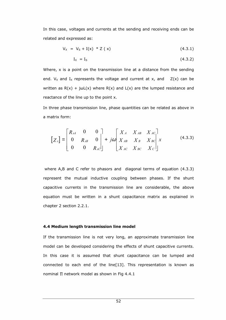
52
In this case, voltages and currents at the sending and receiving ends can be
related and expressed as:
VX = VS + I(x) * Z ( x) (4.3.1)
IX = IS (4.3.2)
Where, x is a point on the transmission line at a distance from the sending
end. VX and IX represents the voltage and current at x, and Z(x) can be
written as R(x) + jωL(x) where R(x) and L(x) are the lumped resistance and
reactance of the line up to the point x.
In three phase transmission line, phase quantities can be related as above in
a matrix form:
(4.3.3)
where A,B and C refer to phasors and diagonal terms of equation (4.3.3)
represent the mutual inductive coupling between phases. If the shunt
capacitive currents in the transmission line are considerable, the above
equation must be written in a shunt capacitance matrix as explained in
chapter 2 section 2.2.1.
4.4 Medium length transmission line model
If the transmission line is not very long, an approximate transmission line
model can be developed considering the effects of shunt capacitive currents.
In this case it is assumed that shunt capacitance can be lumped and
connected to each end of the line[13]. This representation is known as
nominal ∏ network model as shown in Fig 4.4.1
[ ]0 0
0 00 0
xA A AB AC
x xB AB B BC
xC AC BC C
R X X Xj xZ R X X X
R X X Xω
= +
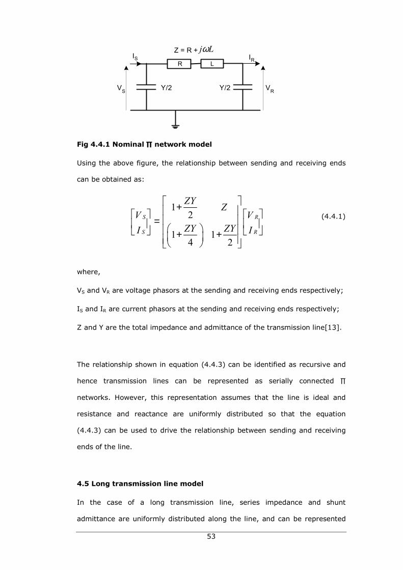
53
Fig 4.4.1 Nominal ∏ network model
Using the above figure, the relationship between sending and receiving ends
can be obtained as:
(4.4.1)
where,
VS and VR are voltage phasors at the sending and receiving ends respectively;
IS and IR are current phasors at the sending and receiving ends respectively;
Z and Y are the total impedance and admittance of the transmission line[13].
The relationship shown in equation (4.4.3) can be identified as recursive and
hence transmission lines can be represented as serially connected ∏
networks. However, this representation assumes that the line is ideal and
resistance and reactance are uniformly distributed so that the equation
(4.4.3) can be used to drive the relationship between sending and receiving
ends of the line.
4.5 Long transmission line model
In the case of a long transmission line, series impedance and shunt
admittance are uniformly distributed along the line, and can be represented
R L
VS VRY/2 Y/2
IS IRZ = R + j Lω
12
1 14 2
S R
S R
ZY ZV V
ZY ZYI I
+ = + +
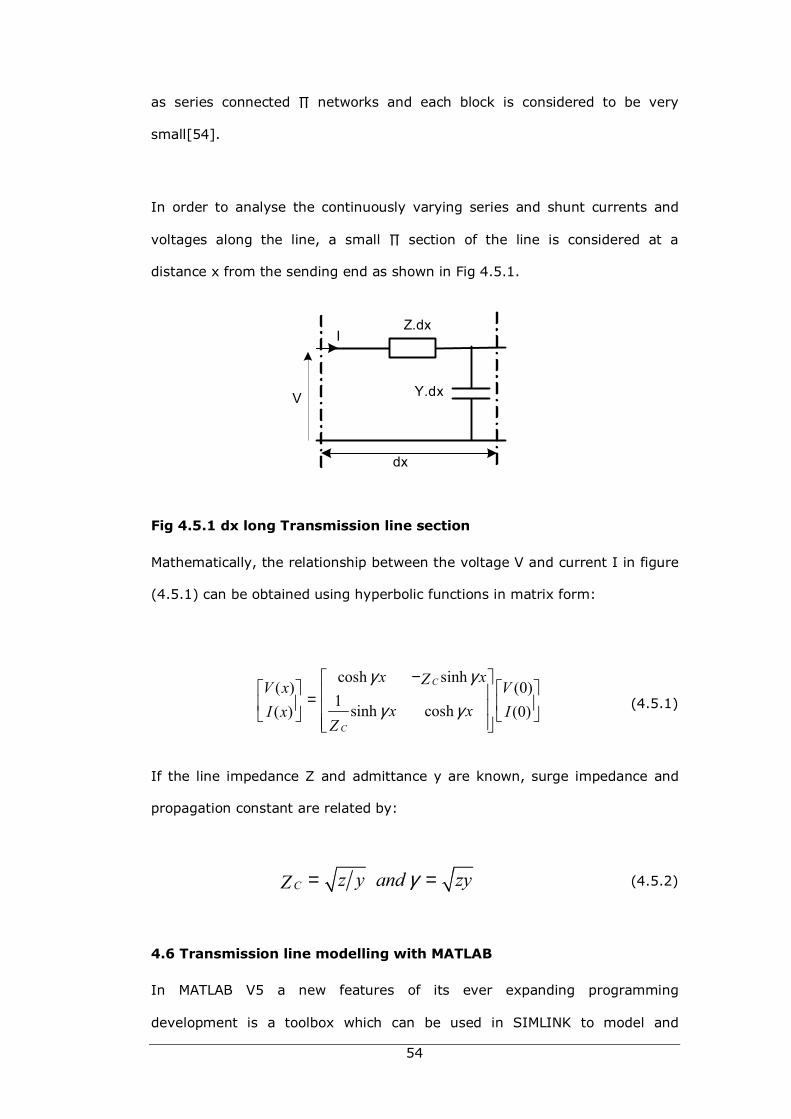
54
as series connected ∏ networks and each block is considered to be very
small[54].
In order to analyse the continuously varying series and shunt currents and
voltages along the line, a small ∏ section of the line is considered at a
distance x from the sending end as shown in Fig 4.5.1.
Fig 4.5.1 dx long Transmission line section
Mathematically, the relationship between the voltage V and current I in figure
(4.5.1) can be obtained using hyperbolic functions in matrix form:
(4.5.1)
If the line impedance Z and admittance y are known, surge impedance and
propagation constant are related by:
(4.5.2)
4.6 Transmission line modelling with MATLAB
In MATLAB V5 a new features of its ever expanding programming
development is a toolbox which can be used in SIMLINK to model and
V Y.dx
IZ.dx
dx
cosh sinh( ) (0)
1 sinh cosh( ) (0)
C
C
x xZV x Vx xI x I
Z
γ γ
γ γ
− =
C z y and zyZ γ= =
55
simulate complex power networks with reasonable accuracy. In this research,
at the beginning, MATLAB 6.5 programming tool Power System Blockset is
used to simulate faults in two ends transmission networks [49]. The
paragraphs below explain how the Power System Blockset can be used on
such transmission network simulations.
4.6.1 Simulink of MATLAB
This part of MATLAB provides the simulation mechanism of many different
engineering applications. Prior to initiating the simulation, a power system
network is developed in Simulink environment, combining different
components in its Power System Blockset tool box[49].
4.6.2 Power system blockset
MATLAB Power System Block set has a number of blocks to create three
phase transmission line network model and simulate in a variety of conditions,
suitable for most of the power system analysis. Once the blocks are selected
and their properties are adjusted in accordance with model parameters, then,
it allows connecting blocks to create the transmission network, ready to run
the simulations.
The blocks in MATLAB are available in following areas of power transmission
networks [49]:
4.6.3 Power system networks
In this category, RLC branches and loads can be modelled together with
circuit breakers, AC voltage and current sources and DC voltage sources. The
transmission line can be modelled as Pi section lines or distributed parameter
lines with mutual inductances. In addition, linear and saturable transformers
can be added to the model.
56
4.6.4 Electric machinery
Synchronous machines can be modelled as complete or simplified models
depend on the required network model. Additional blocks are available for
asynchronous machines and permanent magnet synchronous machines. Other
control blocks are available for hydraulic turbines, governors and excitation
systems.
4.6.5 Measurements and controls
Voltage and current measurements can be implemented in any node or
branch of the network. These measurements can be viewed during the
simulation time using MATLAB scopes [50]. Events can be programmed using
timer control blocks and it allows switching on and off components during the
simulations.
4.6.6 Three-phase power library
In three phase transmission network modelling blocks are available in
following categories:
• Three phase loads and branches
• Pi line sections
• AC voltage sources
• Three-phase transformers in all basic types of configurations
• Three-phase thyristor bridges and diode bridges
When the transmission line network is configured and line data is available,
the above blocks can be combined to create almost any complicated network
for simulation purpose in MATLAB. Another important feature in MATLAB is
57
that new user defined blocks can be built using existing blocks specifying
inputs and outputs for external connectivity.
This technique was quite useful in developing the three phase transmission
line sections and series compensation units. Since there was no three phase
series compensation device available in MATLAB power system block set, a
single line series compensation device with necessary measuring devices was
built using existing blocks as shown in section Fig 3.10.1. This block was
accurately designed with required V-I characteristic of MOV. Then the three
phase series compensation section was made combining together with two
similar blocks.
4.6.7 Simulation controls
For time-domain simulation, the Power System Block set takes advantage of
Simulink's powerful variable-step integrators and zero-crossing detection
capabilities to produce highly accurate simulations of power system models.
In addition, you have access to all of the block building and masking features,
allowing you to build more complex components from electrical primitives
[49].
4.6.8 Signal recording devices
The signal recoding devices in simulink simin and simout was extremely
useful in recording the data signals during the simulation of fault on the
transmission network. Using these blocks, data can be read or written to
MATLAB workspace in array format so that these data will be directly available
for further processing with its script language. If higher data storage is
required, MATLAB can also forward the simulation data to text files. See
more details on theses devices in Full Product MATLAB Help reference [49].
58
4.6.9 Programming with MATLAB
Finally, the MATLAB software provides a broad programming environment
area to create application development. In this research work, most of the
fault location algorithms were developed in the MATLAB programming
environment. Any variables or arrays of data available in the workspace can
be directly used in the application programs and the results generated from
the programs are updated to the same workspace dynamically [49].
The next section describes another power system simulation software used in
the development of the fault location algorithm using time domain signals
which is very well proven and highly accepted in power system research for
modelling power system accurately. Since it was very convenient to use the
MATLAB as the programming environment, the data recording obtained from
simulations run on this software was imported to MATLAB for further
algorithm developments.
4.7 Transmission line modelling with EMTP software
EMTP or Electromagnetic Transients Program was developed in Portland,
Oregon, USA in the early 80s using a FORTRAN style of programming and still
very popular particularly within the research and development community of
power system area, all over the world [53].
Although the EMTP (recently known as ATP) has a proven record for accuracy
of modelling transmission networks, the user friendliness of the software is
still very poor compared to present day software applications. Because of the
above, this software is not commercially available for industry use [47].
ATP is primarily designed based on electromagnetic transient analysis, and it
has other supporting programs such as LINE CONSTANTS, JMARTI SETUP,
59
SEMLYEN SETUP etc. These program results can directly be included in the
ATP main simulation program data case, for further studies on transient
analysis. The input of the ATP consists of data lines which described the
power transmission network and its parameters for the simulation. Since ATP
has been widely used for the fault simulation in this research, it is appropriate
to discuss ATP in some detail[11].
4.7.1 The alternative transient program (ATP)
ATP is used to simulate transients on electrical transmission networks, and is
used to solve the algebraic, ordinary, and/or partial differential equations,
that are associated with interconnections of the following components [11]:
• Lumped resistance, inductance and capacitance
• Multi phase ∏ equivalents, where the preceding scalar R, L, and C
become symmetric, square matrices [R], [L] and [C].
• Multi phase distributed parameter transmission lines, wherein
propagation time of the component is represented. Both constant
parameter and frequency dependent representations are provided.
• Nonlinear resistors, where the V-I characterised is single valued.
• Nonlinear inductors, either with the conventional single valued
characteristics or including hysteresis and residual flux.
• Time varying resistance.
60
• Switches that can be used to simulate circuit breakers spark gaps or
any other connection change networks. Diode and thyristor based
networks are also included.
• Voltage or current sources that can be implemented as single or three
phase. In addition to standard mathematical function blocks, user
defined sources can be implemented specifying discrete data points
representing characteristics of the specific source in conjunction of
TACS (Transient Analysis of Control Systems) controls.
• TACS controls can be included as transfer function blocks to implement
control systems required for the power system components such as
governor or AVR of the generator or other controls required for
stabilisers and TCSC.
• Dynamic rotating machinery, of which the most common form is
conventional three phase synchronous machines. But induction
machinery and dc – machinery also can be represented for single or
multi phases. Such machine models can be connected to TACS control
system model, thereby allowing dynamics for voltage regulators and
speed governors.
4.7.2 EMTP/ATP simulation
EMTP is a full – featured transient analysis program which is mainly developed
for electrical power systems and simulation starts with inputs to the program
using the form of Data case. The basic data structure of the most common
61
method in EMTP simulations with brief description of each data section is
shown in Appendix A-A and A-B.
4.8 Modelling of transmission lines
The EMTP/ATP program has several ways of modelling high voltage
transmission lines and they are namely:
• Using RLC mutually coupled branches or multiphase ∏ network model
• Distributed modelling with constant parameters
• Distributed modelling with frequency dependent parameters
The choosing of the particular model is very much dependent on how the
model is close to the real transmission network and to the level of network
simulation required for the targeted analysis.
For example, if the modelling is required for a short line, RLC mutually
coupled method is quite sufficient for the fault cases such as estimating the
location of the fault. If the study is used on transient analysis in long
transmission line, it is best to use distributed modelling with constant
parameters. In this research work these two methods have been used for
short and long transmission line study cases. The supporting programs in
EMTP/ATP first compute the necessary resistance, inductance and capacitance
matrices from the given transmission line configuration before starting the
simulation process.
4.9 Simulation of faults in EMTP/ATP
In the case of pure resistive faults, an LRC branch can be connected to the
fault point with grounding the other end via switching arrangement. EMTP
switches are implemented defining the status of the switches according to the
fault inception required during the simulation [11].
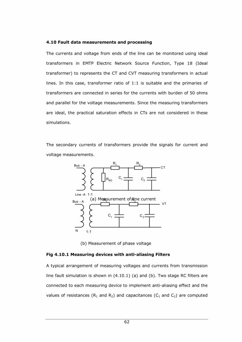
62
4.10 Fault data measurements and processing
The currents and voltage from ends of the line can be monitored using ideal
transformers in EMTP Electric Network Source Function, Type 18 (Ideal
transformer) to represents the CT and CVT measuring transformers in actual
lines. In this case, transformer ratio of 1:1 is suitable and the primaries of
transformers are connected in series for the currents with burden of 50 ohms
and parallel for the voltage measurements. Since the measuring transformers
are ideal, the practical saturation effects in CTs are not considered in these
simulations.
The secondary currents of transformers provide the signals for current and
voltage measurements.
(a) Measurement of line current
(b) Measurement of phase voltage
Fig 4.10.1 Measuring devices with anti-aliasing Filters
A typical arrangement of measuring voltages and currents from transmission
line fault simulation is shown in (4.10.1) (a) and (b). Two stage RC filters are
connected to each measuring device to implement anti-aliasing effect and the
values of resistances (R1 and R2) and capacitances (C1 and C2) are computed
Line -A 1:1
RBD
R1 R2
C1 C2
CTBus - A
1:1
C1 C2
VTBus - A
N
R1 R2
63
based on the sampling frequency with respect to power frequency in the
following manner.
Consider the required sampling rate of signal measurements as 1 KHz and
the power frequency as 50 Hz.
No of samples per second = 1000
No of second for cycle = 0.02 sec
No of samples per cycle = 20
Required filter bandwidth = 500 Hz
Values for Rs ands Cs can be computed in accordance with the given
bandwidth to filter high frequency noise prior to send to the fault location
algorithm.
The sampling time and duration of the simulation in EMTP is controlled by the
special request card as shown in Fig 4.7.1 and has the following general
format [11]:
C ………………………….Miscellaneous data…………………………………….
DaltaT - TMAX -XOPT - COPT - EPSILN - TOLMAX ------
where,
DeltaT: The size of the time step of numerical integration in seconds,
TMAX: Duration of the simulation in seconds,
XOPT: Indicates inductances are given in ohms or in mH,
COPT: Indicates capacitances are given in micro ohms or in mF,
EPSILN: The near zero tolerance for the real coefficient matrix,
TOLMAX: The near zero tolerance for the complex admittance matrix.
64
Other data in this card specifies the parameters for the printing and plotting
outputs.
4.11 Modelling of series compensation
Modelling of very basic series compensation device using MATLAB simulation
package is already covered in Chapter 3 section 9. However more complicated
thyristor switched or controlled devices can be modelled with MATLAB adding
thyristor blocks with control devices to simulated external or internal
controlled reactive VAR injection [49].
This section presents the basic method of simulating series compensation
devices in EMTP/ATP software with various controlling options as they were
required for the fault location algorithm development for the series
compensated transmission lines later in the following chapters.
For example, the standard fixed series capacitor compensating devices has
several components:
• A series capacitor
• MOV device
• Air gap device
• Bypass breaker arrangement
The capacitor of the series compensation device can be easily modelled in
EMTP with LRC branch cards, and MOV with Air gap implementation in EMTP
described as follows:
65
EMTP model for exponential ZnO surge arrester type 92 is quite practicable for
the simulation MOV device and follows the V-I characteristics of non linearity
as:
i = p * (v/Vref)**q (4.11.1)
where I is the MOV current, v is the MOV voltage drop, p, Vref and q are
constants of the MOV device [47]. Data for this device comes in several cards
depending on the implementation of MOV characterises for the study of
simulation. The first data card identifies the data type 92 and other
information of branch connections. The second data contains control
variables:
VREF: The reference voltage of the MOV constraint equation in volts,
VFLASH: The flash over voltage of the air gap in normalised form for VREF
VZERO: The initial MOV voltage at time zero
COL: The number of columns in the MOV device
COEF: The coefficient p of the equation (4.11.1)
EXPON: The exponent of the MOV characteristic equation
VMIN: The minimum voltage for the usage of just-stated characteristics in
p.u.
The exponent segment of the MOV characteristics can be further detailed
adding more data cards to the EMTP type 92.
The bypass breaker arrangement is implemented adding a parallel short
circuit connection with breaker to MOV device with external switching controls
using TACS variables. The pre computed constraint values can be setup for
the triggering of the breaker monitoring the MOV current.
66
4.12 Summary
Mathematical modelling of transmission lines is discussed in detail in order to
lay the foundation of developing a new accurate fault location algorithm for
series compensated transmission lines. It was illustrated that new line
models described in this chapter are capable of handling long transmission
lines, which have significantly higher, shunt capacitive currents. Two different
softwares are used to simulate the power network for testing the newly
developed algorithm and details of modules available in both softwares are
discussed in relation to modelling of power system components including
series compensation devices.
67
Chapter 5.0
Reactive compensation on
transmission lines
5.1 Introduction
The transmission network of a power system is required to deliver both active
and reactive power to the loads on the system. In general both these types of
power are supplied by the power network generators within their MW and
MVAR limits imposed by the design of individual units. The combining of
capacitive and inductive components in the network however leads to the
reduction of the var requirement of a power system, as the leading vars are
opposed by the lagging vars.
This chapter first describes the basics of the reactive power control associated
with high voltage transmission networks and the various methods used in
modern power systems to control the reactive power, and increasing the
power transfer capabilities of the network. Next it deals with the voltage and
transient stability improvements due to the individual reactive control
methods and the discussion is extended to include recently developed FACTS
transmission systems and associated problems in controlling reactive power
[12].
68
5.2 Reactive power control
5.2.1 Fundamental principle
Reactive power is associated with almost all AC circuit and power
systems are no exceptions. The phase shifting of the currents and
voltages during the power transmission causes the reactive power flow
in the transmission networks. The unit of measuring reactive power is
designated as var, and is the volt-ampere reactive, and for a single
phase system is given by:
Reactive power (Q) = V. I. sin θ (5.2.1)
where V and I are the voltage and current of the transmission node
and θ is the phase angle between voltage and current waveforms. The
sign of Q depends on the direction of theta [43]. The net reactive
power supplied to an inductive element is taken as positive and to the
capacitive element as negative.
5.2.2 Two port model
In spite of the complexity of an actual power system, the basic
relationships of the power transmission can be derived by a simple two
port transmission line model with supply sources that are connected to
each end of the line. An ac transmission line is characterised by its
distributed circuit parameters: the series resistance and inductance,
and the shunt capacitance and conductance. The characteristic
behaviour of the line is primarily determined by the reactive circuit
elements, the series inductance l and the shunt capacitance c.
Considering the line series impedance and shunt admittance per meter

69
in ohms as Z and Y, the relationship between sending and receiving
ends voltages and currents can be expressed in matrix form:
(5.2.2)
where A, B, C and D parameters of the network are determined by the
transmission line model as given in table 5.3.1.
Line
Parameter
Exact
Model
Nominal ∏
Model
A or D
B
C
Table 5.2.1 Two port transmission line model
Here l is the length of the line in meters and γ is the propagation constant and
are defined by:
(5.2.3)
where α is attenuation constant (nepers) per meter and β is phase shift
constant ( radians ) per meter.
The characteristic impedance of the line is:
(5.2.4)
S R
S R
A BV VC DI I
=
( )cosh lγ
( )sinhC lZ γ
( )sinhC lY γ
12ZY+
Z
14ZY+
j ZYγ α β= + =
CZ
Z Y=
70
For overhead transmission lines, the velocity of propagation which relates to β
in equation (5.2.2) is very close to the velocity of light [13].
5.2.3 Reactive power elements
Before examining the active and reactive balances of the power network, it is
necessary to discuss the reactive power sources and sinks which are
incorporated with ac power transmission networks.
5.2.3.1 Generators
Under excited generators operate at leading power factors and absorb
reactive power from the network. The purpose of this operation is to help
absorb the system reactive power surplus during light load periods, while
maintaining voltages within prescribed limits. However, var absorption
capabilities of the generators are limited to the stability of the machine and
stator heating limits. On the other hand, generators can be operated at
lagging power factors so that it helps to supply the required reactive power
demand. Either rotor or stator heating imposes limits on var generation
capabilities of alternators.
5.2.3.2 Synchronous compensators
In addition to the generators, synchronous var compensators, which are
basically unloaded synchronous motors, have both var absorption and
generation capabilities. Another variant is the use of clutches, particularly on
gas turbine units, which may be used to decouple the generator from the
turbine and run as a synchronous var compensator.
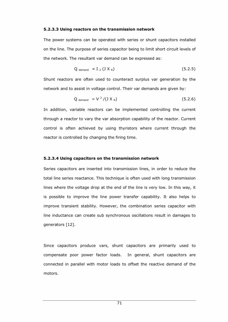
71
5.2.3.3 Using reactors on the transmission network
The power systems can be operated with series or shunt capacitors installed
on the line. The purpose of series capacitor being to limit short circuit levels of
the network. The resultant var demand can be expressed as:
Q demand = I 2 (J X R) (5.2.5)
Shunt reactors are often used to counteract surplus var generation by the
network and to assist in voltage control. Their var demands are given by:
Q demand = V 2 /(J X R) (5.2.6)
In addition, variable reactors can be implemented controlling the current
through a reactor to vary the var absorption capability of the reactor. Current
control is often achieved by using thyristors where current through the
reactor is controlled by changing the firing time.
5.2.3.4 Using capacitors on the transmission network
Series capacitors are inserted into transmission lines, in order to reduce the
total line series reactance. This technique is often used with long transmission
lines where the voltage drop at the end of the line is very low. In this way, it
is possible to improve the line power transfer capability. It also helps to
improve transient stability. However, the combination series capacitor with
line inductance can create sub synchronous oscillations result in damages to
generators [12].
Since capacitors produce vars, shunt capacitors are primarily used to
compensate poor power factor loads. In general, shunt capacitors are
connected in parallel with motor loads to offset the reactive demand of the
motors.
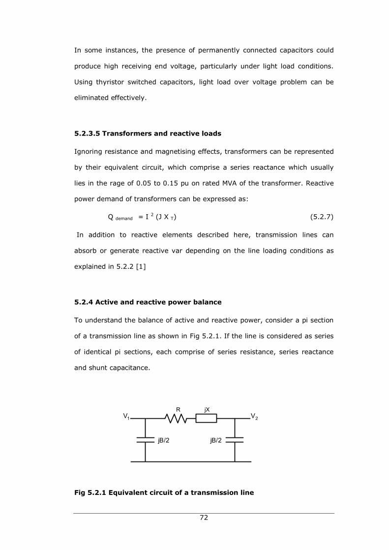
72
In some instances, the presence of permanently connected capacitors could
produce high receiving end voltage, particularly under light load conditions.
Using thyristor switched capacitors, light load over voltage problem can be
eliminated effectively.
5.2.3.5 Transformers and reactive loads
Ignoring resistance and magnetising effects, transformers can be represented
by their equivalent circuit, which comprise a series reactance which usually
lies in the rage of 0.05 to 0.15 pu on rated MVA of the transformer. Reactive
power demand of transformers can be expressed as:
Q demand = I 2 (J X T) (5.2.7)
In addition to reactive elements described here, transmission lines can
absorb or generate reactive var depending on the line loading conditions as
explained in 5.2.2 [1]
5.2.4 Active and reactive power balance
To understand the balance of active and reactive power, consider a pi section
of a transmission line as shown in Fig 5.2.1. If the line is considered as series
of identical pi sections, each comprise of series resistance, series reactance
and shunt capacitance.
Fig 5.2.1 Equivalent circuit of a transmission line
RV1 V2
jB/2 jB/2
jX
73
The reactive elements in the line can either produce or absorb reactive power
depending on line loading conditions. Assuming operation voltage is not
varying alone this section, var generation due to the line shunt capacitors are
also fixed. Then the var absorption is caused by the line reactance, depends
on the loading of the line. The condition at which reactive power generation
and absorption are exactly balanced is called the surge impedance loading
(SIL) condition.
Neglecting the resistance effect SIL can be expressed:
P SIL = V2 √(B/X) MW (5.2.8)
Where V = Line to Line voltage (KV),
B = Susceptance (Siemens/km)
X = Reactance (ohms/km).
If the line loading exceeds this level, it has net var absorption condition.
When loading is less than SIL, it has net var generation condition. Reactive
power surplus or deficit as a function of surge impedance loading can be
shown in Fig 5.2.2.
Fig 5.2.2 Reactive power balance
74
Under steady state conditions, the required reactive power balance can be
obtained in most cases using the reactive elements described in section 5.3.2.
This balance can be quickly disturbed due to the sudden changes of a load or
tripping of a generator, and then the new balance must be restored in a short
time to maintain the power system in a healthy condition. It is good practise
to maintain adequate reactive power resources on the system to compensate
for the loss of var generating sources.
The consequence of failing to restore the var balance during system steady
state or fault condition will result in excessive high or low voltage conditions
which can cause damage to the plant or seriously affect system security.
Reactive power control achieved by adjusting var control elements in the
system may not be fast enough to handle rapid network changes and static
var compensators prove invaluable in these conditions.
5.3 Static VAR compensators
Static var compensators are very popular in controlling reactive power and
are currently used in many power transmission networks all over the world
with many configurations. However, in general SVCs are shunt connected
sinks and/or sources of reactive power and their output may be varied to
maintain or control specific parameters of a power system. For example, by
generating or absorbing reactive power, an SVC can maintain virtually
constant voltage at any particular network node under almost any conditions.
Unlike rotating var compensators, static var compensators do not have inertia
or any moving components, and are mainly power electronics devices which
can act instantly. Since there are no mechanical switching devices or rotating
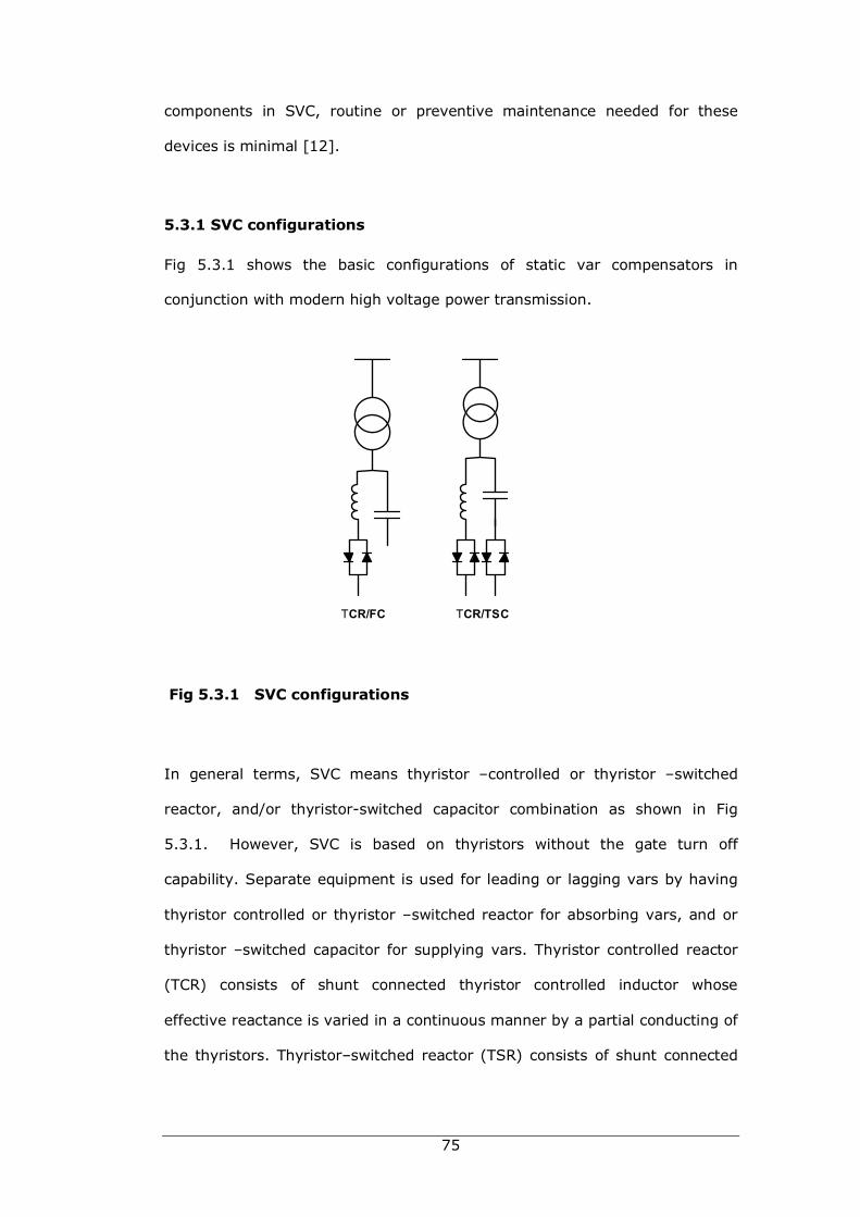
75
components in SVC, routine or preventive maintenance needed for these
devices is minimal [12].
5.3.1 SVC configurations
Fig 5.3.1 shows the basic configurations of static var compensators in
conjunction with modern high voltage power transmission.
Fig 5.3.1 SVC configurations
In general terms, SVC means thyristor –controlled or thyristor –switched
reactor, and/or thyristor-switched capacitor combination as shown in Fig
5.3.1. However, SVC is based on thyristors without the gate turn off
capability. Separate equipment is used for leading or lagging vars by having
thyristor controlled or thyristor –switched reactor for absorbing vars, and or
thyristor –switched capacitor for supplying vars. Thyristor controlled reactor
(TCR) consists of shunt connected thyristor controlled inductor whose
effective reactance is varied in a continuous manner by a partial conducting of
the thyristors. Thyristor–switched reactor (TSR) consists of shunt connected
TCR/FC TCR/TSC
76
thyristor controlled inductor whose effective reactance is varied in a step wise
manner by controlling the on and off turning of thyristors [12, 43].
5.4 Increasing power transfer limits
In general, one of the biggest advantages in using reactive compensation is
that it increases the steady state transmittable power in the transmission
network. An appropriate reactive compensation can be accommodated to
control the voltage profile alone the line, thus increasing the power transfer
capability of the network. The shunt connected fixed or variable reactors are
applied to minimise line over voltage under light load conditions and shunt
connected capacitors applied to maintain voltage levels under heavy load
conditions [45].
In the case of long transmission lines, series capacitor compensation is widely
used to establish a virtual short line by reducing the line reactance where the
electrical length δ could be written as:
δ = (Xl/XC) 1/2 (5.4.1)
where Xl and XC are referred to transmission line reactance and series
capacitance of the series compensation.
5.5 Series VAR compensation
The aim of series capacitive compensation is to decrease the overall effective
series transmission line impedance from the sending end to the receiving end.
Consider the simple two port transmission line model where the series
capacitor is located in the middle of the line so that it forms two identical line
segments on either sides of the capacitor as shown in Fig 5.5.1 (a). The
corresponding voltage and current phasors are shown in Fig 5.5.1 (b) [43].
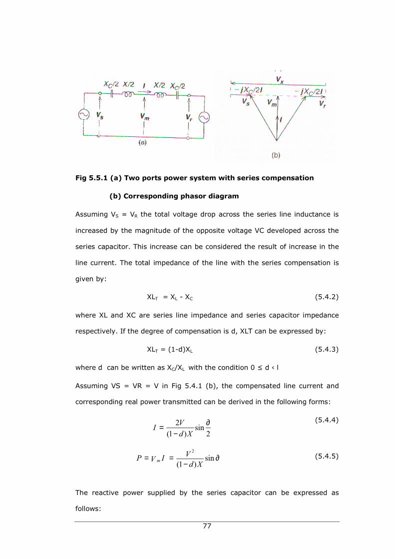
77
Fig 5.5.1 (a) Two ports power system with series compensation
(b) Corresponding phasor diagram
Assuming VS = VR the total voltage drop across the series line inductance is
increased by the magnitude of the opposite voltage VC developed across the
series capacitor. This increase can be considered the result of increase in the
line current. The total impedance of the line with the series compensation is
given by:
XLT = XL - XC (5.4.2)
where XL and XC are series line impedance and series capacitor impedance
respectively. If the degree of compensation is d, XLT can be expressed by:
XLT = (1-d)XL (5.4.3)
where d can be written as XC/XL with the condition 0 ≤ d ‹ l
Assuming VS = VR = V in Fig 5.4.1 (b), the compensated line current and
corresponding real power transmitted can be derived in the following forms:
(5.4.4)
(5.4.5)
The reactive power supplied by the series capacitor can be expressed as
follows:
2 sin(1 ) 2VId X
∂=−
2
sin(1 )mVP IVd X
= = ∂−
78
(5.4.6)
From the equation (5.4.5), it can be seen that the transmittable active power
rapidly increased with the degree of series compensation (d), and similarly,
the reactive power supplied by the series capacitor also increased with d and
varies with angle ∂, similar to line reactive power [12, 43].
5.6 Thyristor controlled and switched capacitors
Thyristor controlled series capacitor arrangement is referred to as TCSC and
has the configuration of thyristor controlled reactors (TCRs) in parallel with a
segment of capacitor bank. The TCSC combination allows the fundamental
frequency capacitive reactance to be smoothly controlled over a wide range
and switched to a condition where the thyristor pair conducts continuously
and inserts an inductive reactance in the line [12, 43].
On the other hand, thyristor switched series capacitor (TSSC) uses thyristor
switches in parallel with a segment of capacitor bank which can be rapidly
remove or inserted on the line in discrete steps.
Fig 5.6.1 shows a basic configuration of TCSC and TSSC series compensation
schemes.
22
22 (1 cos )
(1 )CCkVQ I X X k
= = − ∂−
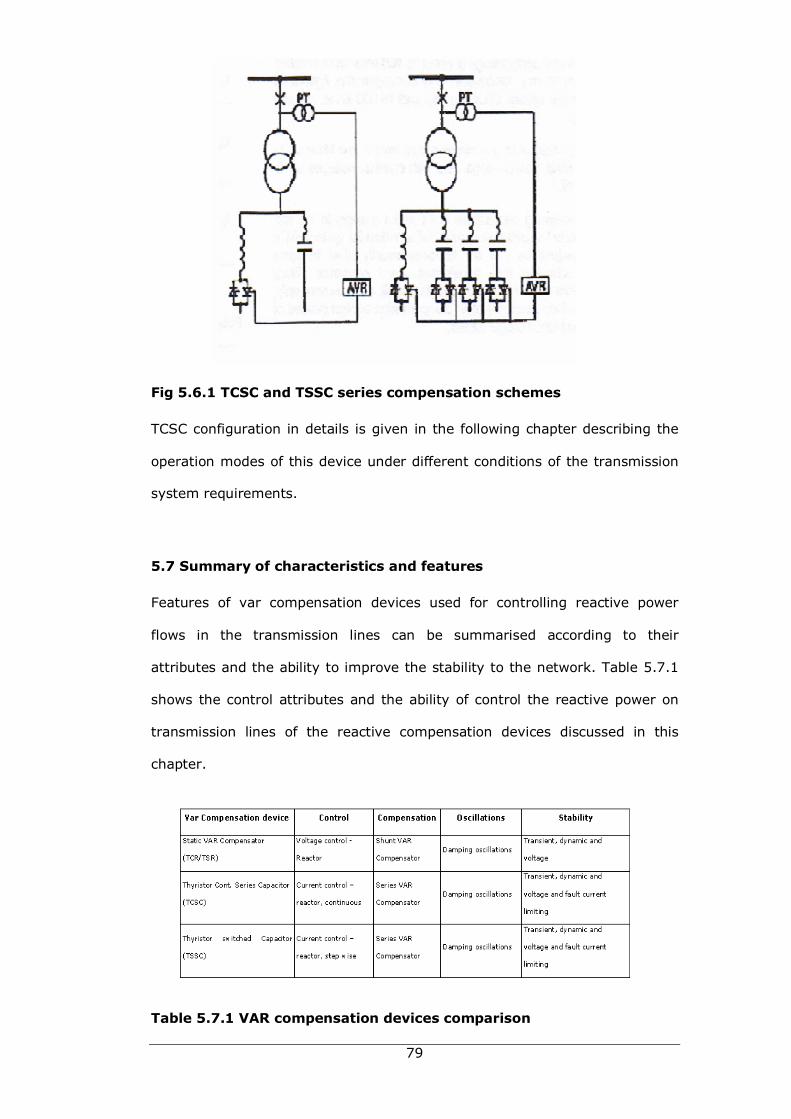
79
Fig 5.6.1 TCSC and TSSC series compensation schemes
TCSC configuration in details is given in the following chapter describing the
operation modes of this device under different conditions of the transmission
system requirements.
5.7 Summary of characteristics and features
Features of var compensation devices used for controlling reactive power
flows in the transmission lines can be summarised according to their
attributes and the ability to improve the stability to the network. Table 5.7.1
shows the control attributes and the ability of control the reactive power on
transmission lines of the reactive compensation devices discussed in this
chapter.
Table 5.7.1 VAR compensation devices comparison
80
5.8 Summary
Power is delivered to the transmission network via generators which provide
the required MW and MVAR power. The reactive power requirements to the
networks can be efficiently managed by connecting VAR compensating
devices with its dynamic controlling features. This chapter describes the basic
reactive power control devices which can be installed in modern power
systems to improve the VAR capabilities of the transmission networks. At the
end of this chapter a comparison of VAR compensating devices according to
their merits is provided.
81
Chapter 6.0
Time domain analysis for
fault location
6.1 Computation of transients
Considering that a fault in a transmission line, introduces transients in voltage
and current of fault signals, and it is difficult and inaccurate to apply a phasor
based approach directly to develop an algorithm in solving problems in
transmission line faults [1, 3]. There are two common methods which can be
applied to solve such problems:
• Frequency domain analysis
• Time domain analysis
6.2 Frequency domain analysis
In this method a steady state analysis of the network consisting of
transmission lines and lumped elements are carried out at a number of
frequencies using transmission network equations for sinusoidal currents and
voltages. Under steady state conditions, at a given frequency, it can be shown
that voltage and current relationship looking from the transmission line source
is expressed in commonly known two port equivalent circuits [13]. These
equitant circuits with voltage and current relations in the lumped elements as
governed by their terminal connections can be resolved to obtain phasor
values of voltage and the current with respect to each node. Then these
82
frequency domain values are combined together using inverse Fourier
transform to convert to time domain transient values with respect to time
[50]. There are number of variations to this method and are called in general
as frequency domain solutions. This method is favoured in solving
transmission line transient problems where line parameters are involved with
frequency dependent components such as shunt capacitance and line
inductances.
However, frequency domain approach is not suitable for solving series
compensated transmission line problems, mainly because the operations are
non linear during the line faults [35]. As the series capacitor voltage rises
beyond a pre-determined over voltage protection during a fault, the
conduction of MOV leads to non linear conditions. Therefore time domain
analysis, which is more suitable for solving problems in series compensated
lines, is discussed broadly in this chapter. Subsequently, new fault location
algorithms for FACTS series compensated transmission lines based on time
domain signals, developed during the further research works on series
compensated transmission is presented in the next chapter [18].
6.3 Time domain analysis
In time domain analysis, voltages and currents in transmission network under
normal or abnormal conditions can be expressed with respect to time, and
these values are known as instantaneous values. Then the time is
incremented by ∆t to get the next set of instantaneous values. Repeating this
process any type of voltage or current signal can be obtained. This time
interval is known as the basic time interval in working with the signals in time
domain analysis. This method is similar to the numerical integration process
and there are a number of ways to implement this in power system transient
problems [55].
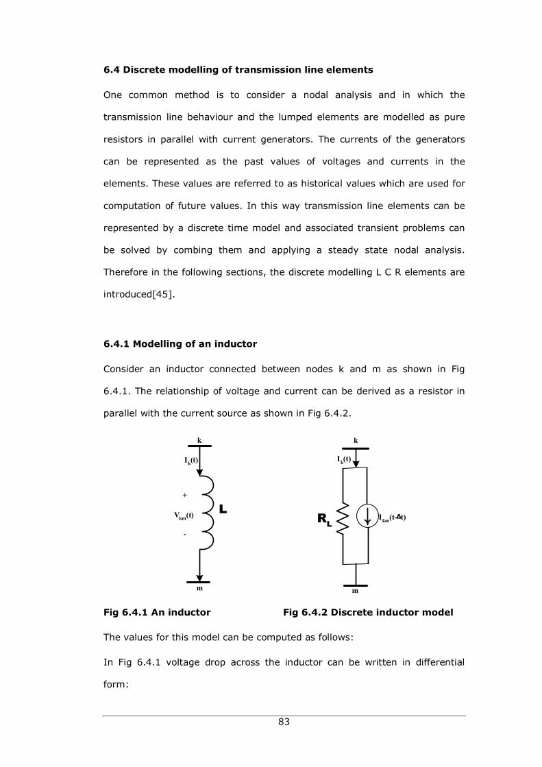
83
6.4 Discrete modelling of transmission line elements
One common method is to consider a nodal analysis and in which the
transmission line behaviour and the lumped elements are modelled as pure
resistors in parallel with current generators. The currents of the generators
can be represented as the past values of voltages and currents in the
elements. These values are referred to as historical values which are used for
computation of future values. In this way transmission line elements can be
represented by a discrete time model and associated transient problems can
be solved by combing them and applying a steady state nodal analysis.
Therefore in the following sections, the discrete modelling L C R elements are
introduced[45].
6.4.1 Modelling of an inductor
Consider an inductor connected between nodes k and m as shown in Fig
6.4.1. The relationship of voltage and current can be derived as a resistor in
parallel with the current source as shown in Fig 6.4.2.
Fig 6.4.1 An inductor Fig 6.4.2 Discrete inductor model
The values for this model can be computed as follows:
In Fig 6.4.1 voltage drop across the inductor can be written in differential
form:
L
Ik(t)
Vkm(t)
k
m
+
-
RL
k
m
Ik(t)
Ikm(t- t)∆
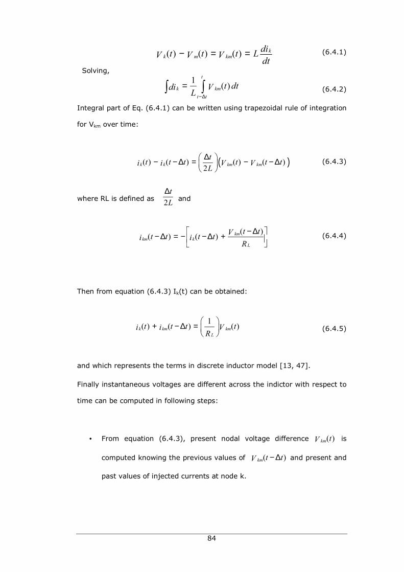
84
(6.4.1)
Solving,
(6.4.2)
Integral part of Eq. (6.4.1) can be written using trapezoidal rule of integration
for Vkm over time:
(6.4.3)
where RL is defined as and
(6.4.4)
Then from equation (6.4.3) Ik(t) can be obtained:
(6.4.5)
and which represents the terms in discrete inductor model [13, 47].
Finally instantaneous voltages are different across the indictor with respect to
time can be computed in following steps:
• From equation (6.4.3), present nodal voltage difference ( )km tV is
computed knowing the previous values of ( )km t tV − ∆ and present and
past values of injected currents at node k.
( ) ( ) ( ) kk m km
dit t t LV V V dt− = =
1 ( )t
k kmt t
t dtdi VL −∆
=∫ ∫
( )( ) ( ) ( ) ( )2k k km kmtt t t t t ti i V VL
∆ − − ∆ = − − ∆
2tL
∆
( )( ) ( ) kmkm k
L
t tVt t t ti iR
− ∆ − ∆ = − − ∆ +
1( ) ( ) ( )k km kmL
t t t ti i VR
+ − ∆ =
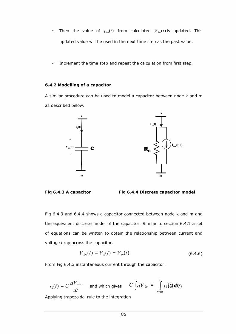
85
• Then the value of ( )km ti from calculated ( )km tV is updated. This
updated value will be used in the next time step as the past value.
• Increment the time step and repeat the calculation from first step.
6.4.2 Modelling of a capacitor
A similar procedure can be used to model a capacitor between node k and m
as described below.
Fig 6.4.3 A capacitor Fig 6.4.4 Discrete capacitor model
Fig 6.4.3 and 6.4.4 shows a capacitor connected between node k and m and
the equivalent discrete model of the capacitor. Similar to section 6.4.1 a set
of equations can be written to obtain the relationship between current and
voltage drop across the capacitor.
(6.4.6)
From Fig 6.4.3 instantaneous current through the capacitor:
and which gives (6.4.7)
Applying trapezoidal rule to the integration
Vkm(t) C
Ik(t)
k
m
+
-RC
Ik(t)
k
m
Ikm (t- t)
( ) ( ) ( )km k mt t tV V V= −
( ) kmk
dVt Cidt
= ( )t
km kt t
C t dtdV i−∆
=∫ ∫
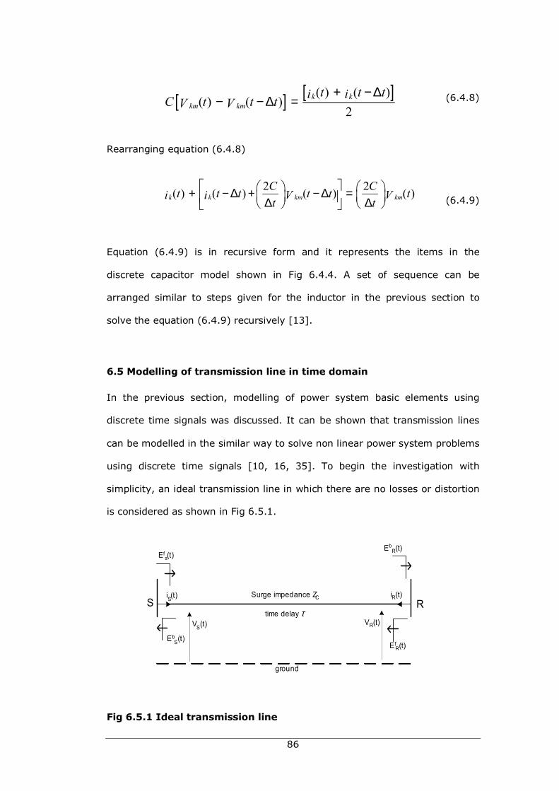
86
(6.4.8)
Rearranging equation (6.4.8)
(6.4.9)
Equation (6.4.9) is in recursive form and it represents the items in the
discrete capacitor model shown in Fig 6.4.4. A set of sequence can be
arranged similar to steps given for the inductor in the previous section to
solve the equation (6.4.9) recursively [13].
6.5 Modelling of transmission line in time domain
In the previous section, modelling of power system basic elements using
discrete time signals was discussed. It can be shown that transmission lines
can be modelled in the similar way to solve non linear power system problems
using discrete time signals [10, 16, 35]. To begin the investigation with
simplicity, an ideal transmission line in which there are no losses or distortion
is considered as shown in Fig 6.5.1.
Fig 6.5.1 Ideal transmission line
[ ] [ ]( ) ( )( ) ( )
2k k
km kmt t ti iC t t tV V
+ − ∆− − ∆ =
2 2( ) ( ) ( ) ( )k k km kmC Ct t t t t ti i V Vt t
+ − ∆ + − ∆ = ∆ ∆
Efs(t)
EfR(t)
EbS(t)
EbR(t)
Surge impedance ZC
time delay τ
ground
iS(t) iR(t)S R
VS(t) VR(t)
87
Using travelling wave concept and ideal transmission line has constant
velocity of propagation v (very close to velocity of light.) and line surge
impedance ZC, and the following behaviour can be observed:
• A step wave travelling from one end travelling to the other end after a
time delay of T which is defined
T = l/v where l is length of the line. The magnitude of the wave is
not reduced during propagation.
• At any given instant t, there are forward and backward travelling
waves in the line and at any point, instantaneous voltage on the line is
given by the summation of the two waves.
• At an end, as time is incremented by one step, the magnitude of the
forward and backward waves are adjusted to produce the correct
terminal voltage and current to satisfy the line equations as well as
terminal conditions of the line.
6.6 Transmission line model relationships with shunt capacitance
As shown in Fig 6.5.1 forward and backward waves are denoted at the
sending end and receiving ends as Efs(t), Eb
s(t), EfR(t) and Eb
R(t) at a given
time t. Then the nodal voltages at each ends can be written as [13, 23]:
(6.6.1)
And
(6.6.2)
Sending end current will be:
(6.6.3)
( ) ( )( ) f bsS s t tt E EV +=
( ) ( )( ) f brR r t tt E EV +=
( ) ( )( )f bs s
SC C
t tE EtIZ Z
= −
88
Receiving end current also is obtained similarly.
From equation (6.6.1), (6.6.2) and (6.6.3) another relationship can be
obtained:
(6.6.4)
Rearranging:
(6.6.5)
Previous sending end current is:
(6.6.6)
Combining equation (6.6.5) and (6.6.6) the following recursive equation is
formed
(6.6.7)
Applying similar logic another recursive formula can be obtained for sending
end current:
(6.6.8)
Similar equations can be obtained for the receiving end voltage and current:
(6.6.9)
(6.6.10)
Relationships of sending and receiving ends voltages and currents formed a
set of recursive formula to compute voltage and current at any point along
the line at any given time t. In Fig 6.6.1 shows these relationships with
respect to the transmission line terminals.
( ) ( )2 bC sS St tIV Z E− =
( )2( ) ( )bs
C SSC
tEt tV Z IZ
= +
[ ]( ) ( ) ( )C S SS t t tV Z I I τ= + −
( ) ( )2 2( )b bs s
SC C
t tE EtIZ Z
ττ −=− =
2( ) ( ) ( )S RRC
t t tVI IZ
τ = − −
[ ]( ) ( ) ( )C R RR t t tV Z I I τ= + −
2( ) ( ) ( )R SSC
t t tVI IZ
τ = − −
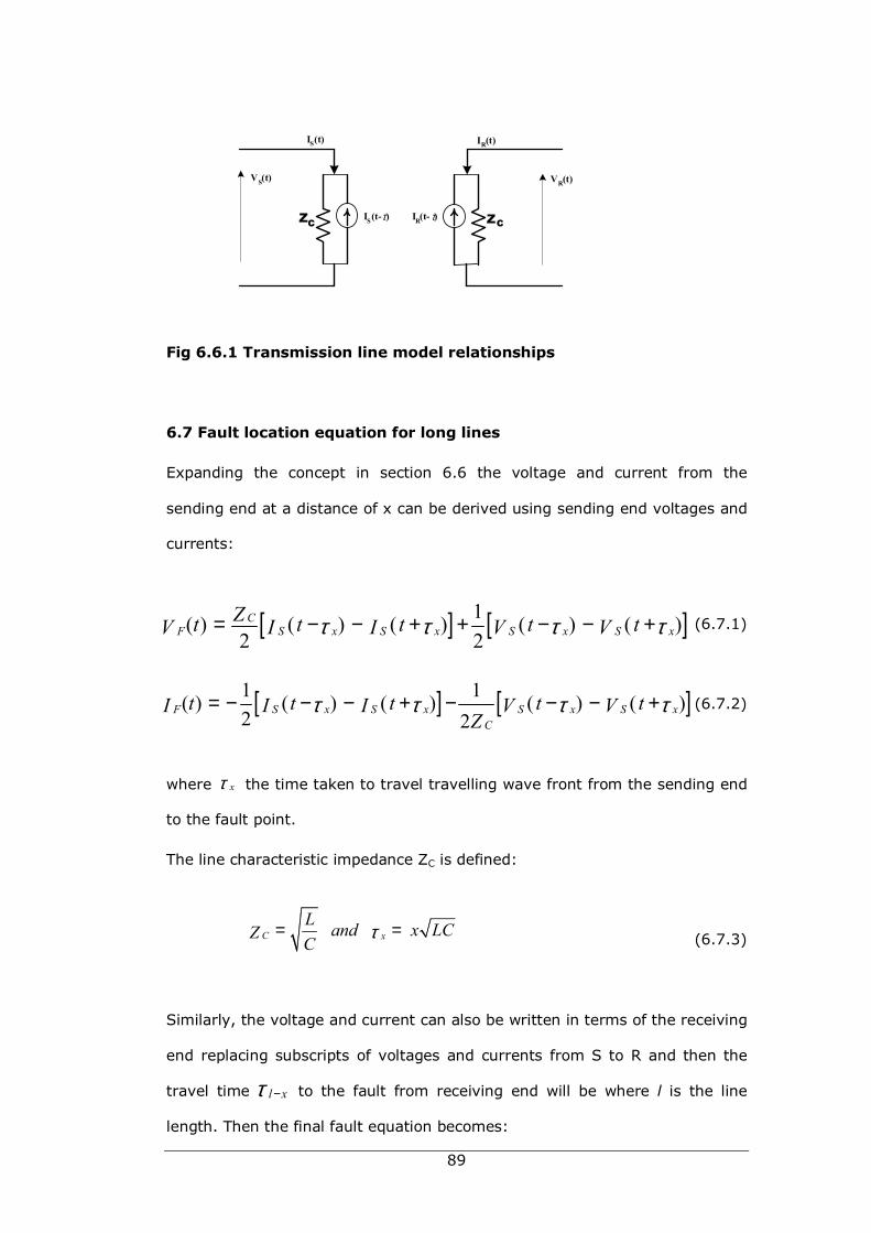
89
Fig 6.6.1 Transmission line model relationships
6.7 Fault location equation for long lines
Expanding the concept in section 6.6 the voltage and current from the
sending end at a distance of x can be derived using sending end voltages and
currents:
(6.7.1)
(6.7.2)
where the time taken to travel travelling wave front from the sending end
to the fault point.
The line characteristic impedance ZC is defined:
(6.7.3)
Similarly, the voltage and current can also be written in terms of the receiving
end replacing subscripts of voltages and currents from S to R and then the
travel time to the fault from receiving end will be where l is the line
length. Then the final fault equation becomes:
IS(t- )ZC
IS(t)
VS(t)
IR(t- ) ZC
IR(t)
VR(t)
τ τ
[ ] [ ]1( ) ( ) ( ) ( ) ( )2 2C
S SF x x S x S xZt t t t tV V VI Iτ τ τ τ= − − + + − − +
[ ] [ ]1 1( ) ( ) ( ) ( ) ( )2 2
F S Sx x S x S xC
t t t t tV VI I IZ
τ τ τ τ= − − − + − − − +
xτ
C xL and x LCZC
τ= =
l xτ −
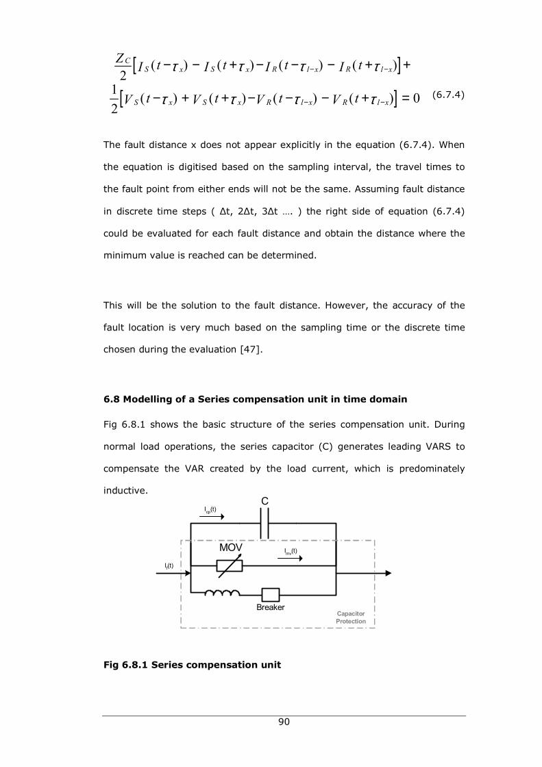
90
(6.7.4)
The fault distance x does not appear explicitly in the equation (6.7.4). When
the equation is digitised based on the sampling interval, the travel times to
the fault point from either ends will not be the same. Assuming fault distance
in discrete time steps ( ∆t, 2∆t, 3∆t …. ) the right side of equation (6.7.4)
could be evaluated for each fault distance and obtain the distance where the
minimum value is reached can be determined.
This will be the solution to the fault distance. However, the accuracy of the
fault location is very much based on the sampling time or the discrete time
chosen during the evaluation [47].
6.8 Modelling of a Series compensation unit in time domain
Fig 6.8.1 shows the basic structure of the series compensation unit. During
normal load operations, the series capacitor (C) generates leading VARS to
compensate the VAR created by the load current, which is predominately
inductive.
Fig 6.8.1 Series compensation unit
C
MOV
BreakerCapacitorProtection
If(t)
Icp(t)
Imv(t)
[ ]( ) ( ) ( ) ( )2C
S S R Rx x l x l xZ t t t tI I I Iτ τ τ τ− −− − + − − − + +
[ ]1 ( ) ( ) ( ) ( ) 02 S x S x R l x R l xt t t tV V V Vτ τ τ τ− −− + + − − − + =
91
The Metal Oxide Varistor (MOV) protection, is connected directly in parallel
with the series capacitor, and operates when its voltage exceeds the
protective voltage level of the capacitor. Therefore in normal operations MOV
acts as an open circuit and does not influence load currents. During fault
conditions, excessive voltage is developed in the capacitor due to the fault
current, which is controlled and limited by the conduction of the MOV unit.
The highly non-linear resistance characteristics of the MOV make it difficult to
estimate the voltage drop across the capacitor. Further, if the fault current is
too high, MOV conduction results in higher absorption of energy, which can
cause the Circuit Breaker to operate, bypassing the capacitor [14].
As shown in Fig 6.8.1, if the fault current passing through the series
compensation unit (SCU) is If, under any operational conditions it can be
shown that:
(6.8.1)
Where Icp and Imv refer to the current passing through capacitor and the MOV
at any given time [16].
6.8.1 Series capacitor voltage drop when MOV is not conducting
Under normal load conditions, line current Il = Icp and Imv = 0; Under fault
conditions, when current passing through the capacitor reaches its protective
level Ipr, MOV will begin conducting. Therefore, it is clear that when the line
current goes from normal load current to fault current, before the conduction
of MOV, the relationship to the fault current is [35]:
(6.8.2)
( ) ( ) ( )f CP MVt t tI I I= +
( ) ( )f CPt tI I=
92
Where Ip.u. < 0.98, Ip.u and Ip.u. is defined as f
pr
II
If the fault current is known, the voltage drop across the capacitor can be
expressed in terms of instantaneous values:
(6.8.3)
Where Vcp(t) is the current voltage drop, and T is the sampling time of the
measured fault current.
By applying the Trapezoidal Rule, the integral part in equation (6.8.3) can be
expressed in terms of the sampled currents as follows:
(6.8.4)
The equation (6.8.4) is a recursive formula and instantaneous capacitor
voltage can be progressively estimated knowing the fault current sample
values [10, 56, 57]. However, one problem is that what initial conditions
could be used to start this recursive estimation of capacitor voltage drop?
The answer to this problem with detailed explanations with implementation
results are given in Chapter 7, where the development of fault location
algorithms using time domain analysis is presented[14].
6.8.2 Modelling of MOV current
To improve the estimation of series capacitor voltage drop while MOV is
conducting, current through the MOV must be considered. Assuming other
protection devices are not in operation the fault current has two paths as
shown in Fig 6.4.1 in the following form:
(6.8.5)
[ ])()(2
)()( TttCTTtt IIVV ffcpcp
−++−=
dttC
Tttt
Tt Fcpcp iVV )(1)()( ∫−+−=
( ) ( ) ( )f CP MOVt t tI I I= +
93
where ICP(t) and IMOV(t) are the instantaneous currents through the capacitor
and the MOV.
As described in Chapter 3 section 6, MOV V-I relationship can be
approximated to polynomial form:
(6.8.6)
According to equation (6.8.6), at any given time, if the voltage across the
series compensator is known the current through the MOV can be found. By
linearising the MOV characteristics around a previous time sample, new
sample values can be estimated from [11]:
(6.8.7)
where IMV(t) and VMV(t) are current and voltage of MOV at time t, respectively,
and IMV(t-T) and VMV(t-T) are pervious sample values. The gradient g is
inversely proportional the slope of MOV characteristic which can be derived
taking the derivative of equation (6.8.6) with respect to voltage
and has the following form:
(6.8.8)
Since the t-T is the sampling interval practically small, this computation is
valid even when the MOV characteristic is non linear. However, the gradient is
not a constant and therefore it must be calculated during each time step to
get accurate results for the MOV instantaneous voltage drops [10].
=VREFVpi
q
*
[ ])()()()( TttgTtt VVII mvmvmvmv −−+−=
−=
−
VREFTt
VREFqpg V mv
q)(*1
94
The relationship between the current through the capacitor and its voltage
drop is given by equation (6.8.4) is still valid, and substituting in equation
(6.8.5) the following expression can be obtained for the instantaneous fault
current:
(6.8.9)
At any given time when capacitor and MOV are conducting:
(6.8.10)
Therefore substituting VMV with VCP in equation (6.8.9)
(6.8.11)
In equation (6.8.9) IMV(t-T) and VCP(t) are unknown and using equations
(6.8.4) and (6.8.5) IMV(t-T) can be found as:
(6.8.12)
Substituting equation (6.8.10) in (6.8.9) final form of fault current can be
obtained as:
(6.8.13)
[ ] +−+−−+−= )2()()()()( TtTttTCTtt VVVII cpcpcpff [ ])()( Tttg VV cpcp −−
[ ] [ ]( ) ( ) ( ) ( ) ( ) ( )f MV MV MV CP CPCt t T g t t T t t Ti i V V V VT
= − + − − + − −
[ ] [ ]( ) ( ) ( ) ( ) ( ) ( )f MV CP CP CP CPCt t T g t t T t t Ti i V V V VT
= − + − − + − −
[ ]( ) ( ) ( ) ( )MV f CP CPCt T t T t t Ti i V VT
− = − − − −
( ) ( ) ( ) ( )CP MV CP MVt t and t T t TV V V V= − = −
95
In this expression if the instantaneous fault current through series
compensator is known, instantaneous voltage drop across the device can be
estimated recursively. As indicated in the pervious section, the initial starting
point is required for the computation of progressive voltages.
Another important issue in this computation is that linearization assumed in
algorithm will not be accurate near the knee point of the MOV characteristics,
where at this point MOV current increases rapidly in a small change in voltage
drop. Another readjustment is required when the capacitor is about to exceed
its protection level in this computation.
6.9 Modelling of TCSC devices
In the previous sections, simple series compensation with the main protection
device MOV is considered for estimation of instantaneous voltage drop across
the device using known through current. This method could be further
improved for the case of more advanced thyristor control switch capacitors
which are used for series compensation [18].
Before considering the thyristor control branch it is more convenient to
mention the other protection devices in the series compensation device.
6.9.1 Spark gaps
During the 1970’s the power gap is used as the primary means of providing
over-voltage protection of the series capacitor. When the voltage across the
capacitor exceeds a specific level, air gap sparked and fault current is diverted
through the air gap to protect the capacitor. Usual values of protection levels
are 2.5 to 4.0 times the normal operating voltage [58].
96
A reactor is placed in series with the gap to limit the capacitor discharge
current through the gap. Once the current flow starts, a parallel bypass switch
is closed to extinguish the arc in the gap. This sequence of operation is
somewhat similar to the MOV protection described in the previous section.
However, V-I characteristics device does not follow a polynomial equation as
in MOV operation [18].
Most of the series compensation devices are equipped with spark gap to
protect the MOV if the through current persists for a longer time where the
energy dissipated exceeds its rated value. In this case, fault current through
the series components are completely by-passed by the operation of air gap.
The energy protection level can be pre-determined knowing the
characteristics of the series compensation device. This level largely depends
on the magnitude and duration of the fault current through the MOV device.
6.9.2 Bypass breaker
The main purpose of the bypass breaker arrangement is to completely bypass
the series compensation device in the case of failure or malfunction of any of
its components. In TCSC arrangements an additional breaker is provided to
eliminate the voltage drop across the TCSC during the energisation.
However, the occurrence of such an event is extremely rare in practical
situations; the fault location algorithm may not require improvements to
consider such a case [58].
6.9.3 Thyristor controlled reactance
The main function of this device in the TCSC is to provide inductive reactance
control to the series capacitor during all possible operating conditions, and to
97
protect series compensation devices from faults. There are several operating
conditions that could be defined with respect to the firing of thyristor branch:
• Normal voltage reversals for a wide range of line currents
• Bypass of the MOV if the energy absorbed exceeded its limits
• Avoid blocking of the thyristor against high voltage
• Continuous bypass of the series capacitor for wide range of line
currents
During a fault period, TCSC switched on to several operation modes
depending on the protection requirement of the series capacitor [43, 58]:
6.9.3.1 Vernier mode
In high impedance fault cases, TCSC is continuously in this mode of normal
operation. Therefore, the protection function of the TCSC device is not
operating and the thyristor valve is fired at a pre-determined firing angle. In
this case TCSC operates as variable impedance. Under this condition, the
system is subjected to sub synchronous resonance oscillations.
6.9.3.2 Block mode
During over voltage conditions, TCSC detects and stops its firing sequence
and the thyristor branch is blocked from normal operation. In this case TCSC
operates as a basic series capacitor with MOV protection device. Since the
high resistance introduced by the MOV operation, the subsynchronous
resonance will decrease in voltage and current signals with exponential decay
98
of DC offset. Therefore TCSC can be modelled for the fault location algorithm
as described in section 6.9.
6.9.3.3 Bypass mode
When the energy absorbed in the MOV exceeds its limitations, the thyristor
control branch switches from block mode to bypass mode, to protect the
series capacitor and the MOV from over voltage condition. In this mode, the
thyristor valve conducts in the complete cycle and it operates as a small value
inductance. Since the voltage and current signals will only contain an
exponential dc off set in this case, TCSC can be considered as pure
inductance.
If the operation characteristic of TCSC is known, then instantaneous voltage
drop across the series capacitor can be estimated similar to section 6.8 with
minor modifications. Since the fault current through the TCSC is monitored
during entire fault period, it will not be difficult to detect the operation mode
of TCSC in order to estimate the TCSC voltage drop [12].
6.10 Summary
Faults in a transmission line introduce transients in the network and therefore
location of fault can not be accurately estimated using algorithm developed by
phasor based approach. Therefore, this chapter introduced frequency domain
analysis and time domain analysis, and how to solve the faulted network
equations in order to estimate fault locations. Then modelling of series
compensated devices using new approaches are explained. This chapter
forms the basis for developing of new fault location algorithms using time
domain approach described in the next chapter.
99
Chapter 7.0
Algorithms for Locating Faults on
Series Compensated Transmission
Lines
7.1 Introduction
In chapter three, a new fault location algorithm for series compensated
transmission networks[1] using phasor based approach was discussed in
detail and the problems associated with implementation issues and how these
issues affect the results are investigated. Also, it was noted that the accuracy
of fault location using phasor based algorithms was severely limited by the
non-liner operation of the series compensation protection devices [2].
In this chapter, a new algorithm for locating faults on series compensated
transmission lines based on time domain approach is described. It was shown
that the new algorithm can estimate the fault location with high accuracy in
comparison to the results obtained with phasor based algorithm. [14].
In this new method, the series compensation voltage drop using
instantaneous fault signals are estimated prior to the estimation of fault
location. The estimated values are applied to the faulted network to estimate
the fault distance solving of time domain signals.
100
Then discussed the practical issues in the implementation of this algorithm in
different transmission line configurations and proposed methods to maintain
the high accuracy of fault location estimation.
In addition, a novel method for improving the algorithm using one end fault
data to estimate the fault distance in series compensated transmission lines
was presented in this chapter. A two port transmission network similar to the
previous cases have been modelled using EMTP/ATP software and the
collected fault data used in the new algorithm to estimate the fault distance.
Finally, the fault location algorithm was tested for time varying fault
resistance issue and it was shown that the accuracy of the fault distance
estimations is high compared to previous results [16, 57]. A case study is
presented, with details of each implementation of the new algorithm in
various line configurations and different fault cases.
7.2 System transients during faults
The previous chapter discussed how to model transmission lines and
associated components using instantaneous time domain signals. For an
example, if the fault current samples are known the instantaneous voltage
drop across an inductor or a capacitor can be estimated recursively. This
method of computation is quite appropriate for transmission line problems
associated with system transient where decaying DC current component is
significant for the accuracy consideration of the application.
During a fault, the series capacitor in series compensated transmission line
will generate an AC transient of the current on fault inception, instead of
decaying DC components of the current associated with most fault angles.
101
The frequency of the transient components of the current will be
approximately equal to:
* Fundamental frequency (7.2.1)
where XC is the total capacitive impedance in series with the total impedance
in inductive impedance [18].
Therefore, in developing a fault location algorithm the system transients
generated in fault signals cannot be filtered or neglected.
7.3 Two ends fault location algorithm using time domain analysis
Consider a parallel arrangement of an ideal capacitor (SC) and a non linear
resister (MOV) as shown in Fig 6.8.1. Assume that the fault current is higher
than the protective level of series capacitor voltage drop such that MOV
operates to divert the portion of fault current from the series capacitor. The
V-I characteristics of the MOV can be expressed by the following non linear
equation [1]:
(7.3.1)
where P and VREF are reference quantities of the MOV and q is the
exponential of polynomial, typically in the order of 20 to 30.
Using instantaneous values, the through current in this component:
If(t) = ICP (t) + IMV (t) (7.3.2)
where ICP and IMV are the currents through the SC and MOV respectively at
time t.
Under normal load, IMV is zero and therefore:
*CP
q
MOVREF
VPI
V=
12
C
L
X
X
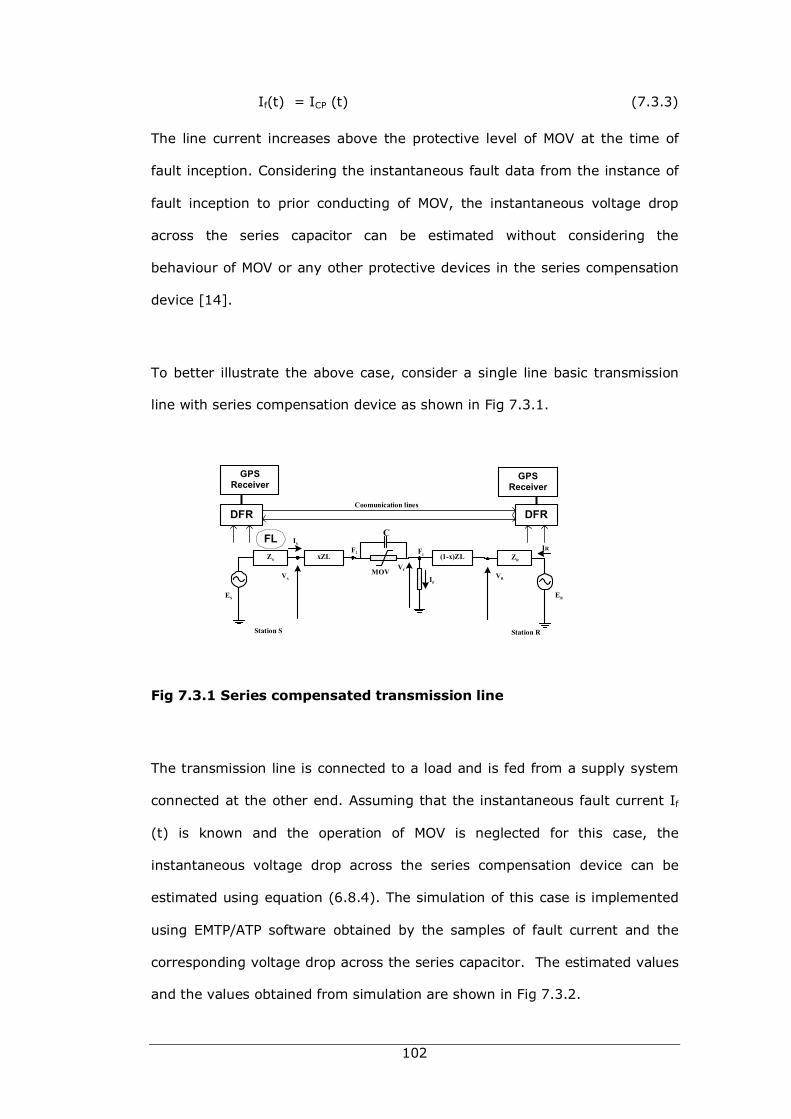
102
If(t) = ICP (t) (7.3.3)
The line current increases above the protective level of MOV at the time of
fault inception. Considering the instantaneous fault data from the instance of
fault inception to prior conducting of MOV, the instantaneous voltage drop
across the series capacitor can be estimated without considering the
behaviour of MOV or any other protective devices in the series compensation
device [14].
To better illustrate the above case, consider a single line basic transmission
line with series compensation device as shown in Fig 7.3.1.
Fig 7.3.1 Series compensated transmission line
The transmission line is connected to a load and is fed from a supply system
connected at the other end. Assuming that the instantaneous fault current If
(t) is known and the operation of MOV is neglected for this case, the
instantaneous voltage drop across the series compensation device can be
estimated using equation (6.8.4). The simulation of this case is implemented
using EMTP/ATP software obtained by the samples of fault current and the
corresponding voltage drop across the series capacitor. The estimated values
and the values obtained from simulation are shown in Fig 7.3.2.
(1-x)ZL
MOV
C
VF
F2
IF
F1
Station R
ES
Station S
ZS xZL
IS
VS
FLZR
ER
IR
VR
GPSReceiver
DFR
GPSReceiver
DFRCoomunication lines
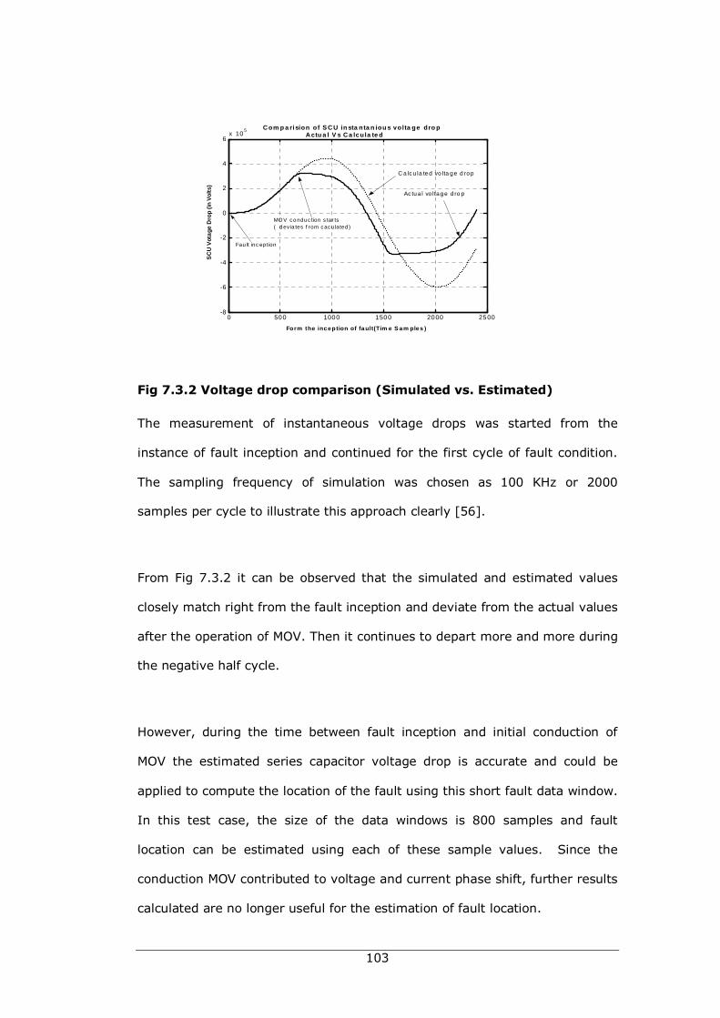
103
Fig 7.3.2 Voltage drop comparison (Simulated vs. Estimated)
The measurement of instantaneous voltage drops was started from the
instance of fault inception and continued for the first cycle of fault condition.
The sampling frequency of simulation was chosen as 100 KHz or 2000
samples per cycle to illustrate this approach clearly [56].
From Fig 7.3.2 it can be observed that the simulated and estimated values
closely match right from the fault inception and deviate from the actual values
after the operation of MOV. Then it continues to depart more and more during
the negative half cycle.
However, during the time between fault inception and initial conduction of
MOV the estimated series capacitor voltage drop is accurate and could be
applied to compute the location of the fault using this short fault data window.
In this test case, the size of the data windows is 800 samples and fault
location can be estimated using each of these sample values. Since the
conduction MOV contributed to voltage and current phase shift, further results
calculated are no longer useful for the estimation of fault location.
0 500 1000 1500 2000 2500-8
-6
-4
-2
0
2
4
6x 10
5
Form the inception of fault(Tim e S am ples )
SC
U V
otag
e D
rop
(in V
olts
)
Ac tua l vo ltage d ro p
C a lc u la ted vo lta ge d rop
MOV c o ndu c tion s tar ts ( d ev ia tes f rom c ac u lated )
Fau lt inc eption
C om p a rision of S C U in sta nta n iou s volta ge dro p A ctu a l V s C a lcula te d
104
7.4 Development of fault location algorithm
The new fault location algorithm was developed using time domain signals
considering various aspects of issues in respect of:
• Complexity of series compensation device
• Fault data measuring from two ends and one end
• Time varying fault cases
Each of these cases is discussed in detail in the following sections, considering
the other practical issues in developing the new algorithm and how the fault
location and resistance can be estimated using time domain analysis [1, 6,
18, 19, 37, 39].
7.5 Fault location
Let us consider the configuration of two terminals transmission line as shown
in Fig 7.3.1.
Assume that the fault occurs at a distance of x kilometres from the local bus,
before the location of series compensation device.
If the voltages and currents at local and remote buses are VS, IS VR and IR,
respectively, the network equation of the faulted system can be written in
matrix form:
(7.5.1) [ ] [ ][ ] [ ] [ ] [ ][ ](1 )S Rs D RL Lx Z x ZV V VI I− − = − −
105
where VD is the voltage drop across the series capacitor which is denoted by
3x1 column matrix and each row represents phasors a, b and c for three
phase network.
The ZL is line impedance matrix which could be represented with dimension of
3x3, where elements of the self and mutual inductance among three phases:
(7.5.2)
IN general, three phase voltage sources can be expressed in matrix form to
match with the equation (7.5.1) and (7.5.2):
(7.5.3)
If the fault occurs on the other side of the network with reference to series
compensation device, only the remote fault current (IR) will be forced through
the device. In this case, the voltage drop across the series capacitor is
estimated using the remote fault current, and equation (7.5.1) can be slightly
modified considering the reversal of fault current [2].
(7.5.4)
The final expression for the fault distance x can be obtained from equations
(7.5.1) or (7.5.2) using instantaneous values monitored at time t0:
(7.5.5)
or
(7.5.6)
[ ]
=
ZZZ
ZZZ
ZZZ
LssLmmLmm
LmmLssLmm
LmmLmmLss
LZ
[ ]EEEE scsbsaT
S =
[ ] [ ][ ] [ ] [ ] [ ] [ ](1 )S Rs R DL Lx Z x ZV V VI I− = − − −
)()()()()()()(
00
00000
tVZtVZtVZtVtVtV
txRS
RDBA
+++−
=
)()()()()()(
)(00
00000
tVZtVZtVZtVtVtV
txRR
RDBA
++−−
=
106
7.6 Series capacitor voltage drops
Considering the three phases, the series capacitor voltage drop VD can be
written in matrix form as follows:
(7.6.1)
where A, B and C refer to the three phases. Since there is no mutual
interaction between the phases, the off diagonal terms of the [VD] are all
zeros. If the fault is involved with fewer number of phases such as 2PG or
1PG, then the diagonal element corresponding to healthy phases are zero.
This is a good practical assumption, as the line load currents are very much
smaller to the fault current. Also, it is worth while to mention that the series
capacitive reactance no needs to be equal in all phases as shown in equation
(7.6.1). The diagonal terms defining capacitor voltage drop with respect to
each phase is derived using fault current in each phase as described in section
7.3 [6, 14].
7.7 Inductive voltage drops
As seen from equation (7.5.5) there are two inductive voltage drops [ZL][IS]
and [ZL][IR] that need to be estimated for each sample, before computing
the fault distance. For an example, first consider the matrix equation of
[ZL][IS] before estimating the instantaneous inductive voltage drops [14].
(7.7.1)
[ ][ ]
[ ][ ]
0 00 00 0
C A
C BD
C C
X IV X I
X I
=
[ ][ ]LS Lm Lm SA
Lm LS Lm SB
Lm Lm LS SC
Z Z Z IZL IS Z Z Z I
Z Z Z I
=

107
where ZLS and ZLM are self and mutual inductance of the transmission line
phase conductors. In this case it is assumed that the entire transmission line
is ideally transposed such that self and mutual inductance of each phase is
identical. From equation (7.7.1) there are number of resistive and inductive
voltage drops to be estimated for the [ZL][IS]:
For diagonal terms:
[XLS][ISA] - Self inductance of the line with phase A current
[RLS][ISA] - Resistance of the line with phase A current
[XLS][ISB] - Self inductance of the line with phase B current
[RLS][ISB] - Resistance of the line with phase B current
[XLS][ISC] - Self inductance of the line with phase C current
[RLS][ISC] - Resistance of the line with phase C current
For off diagonal terms:
[XLM][ISA] - Mutual inductance of the line with phase A current
[ZLM][ISB] - Mutual inductance of the line with phase B current
[ZLM][ISC] - Mutual inductance of the line with phase C current
where RLS and XLS are series resistance and self inductance of the line.
The instantaneous resistive voltage drops are easier to compute using phase
currents of the line and instantaneous inductive voltages can be computed
solving associated deferential equations for self and mutual inductive
components of the line.
In this way, the fault distance can be computed using equations 7.5.5 for
each time sample recorded after the fault inception [6, 14].
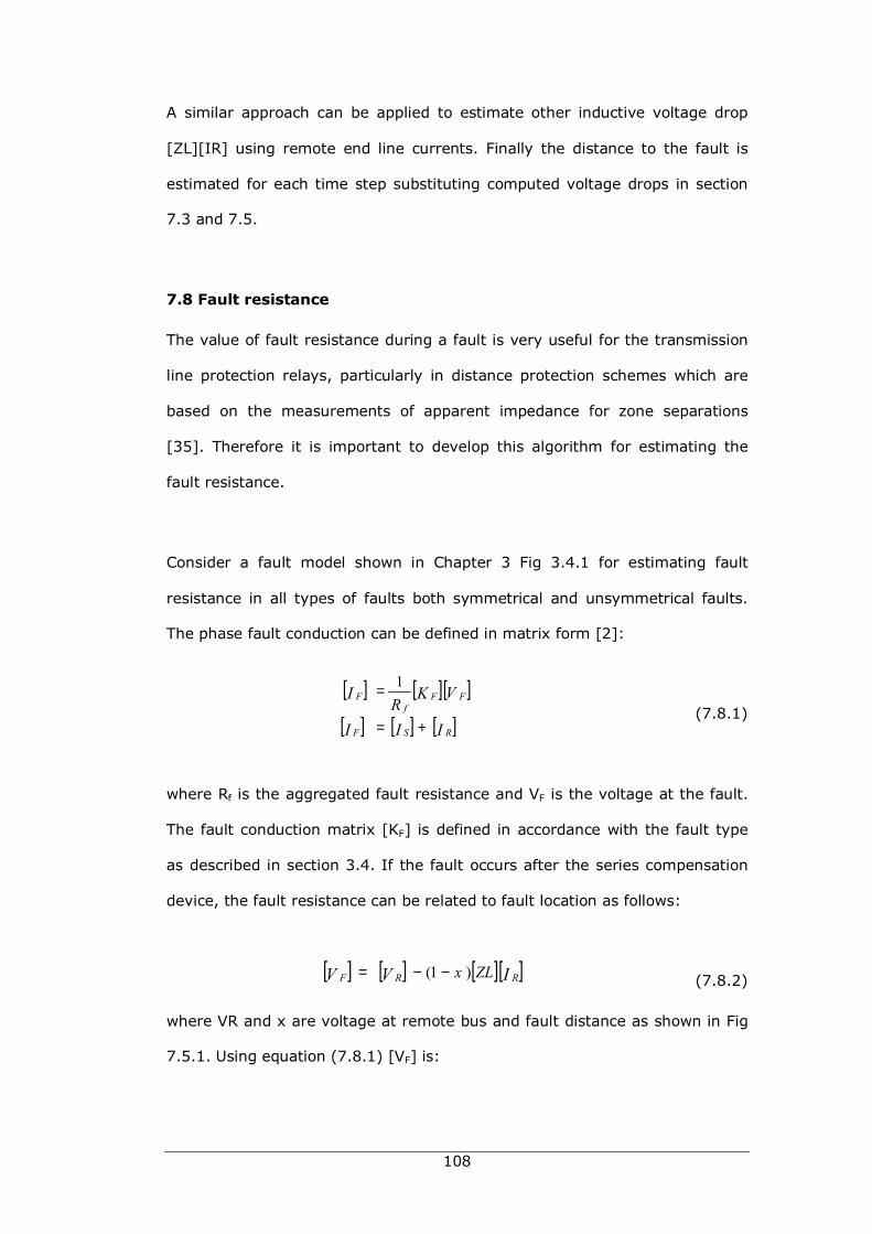
108
A similar approach can be applied to estimate other inductive voltage drop
[ZL][IR] using remote end line currents. Finally the distance to the fault is
estimated for each time step substituting computed voltage drops in section
7.3 and 7.5.
7.8 Fault resistance
The value of fault resistance during a fault is very useful for the transmission
line protection relays, particularly in distance protection schemes which are
based on the measurements of apparent impedance for zone separations
[35]. Therefore it is important to develop this algorithm for estimating the
fault resistance.
Consider a fault model shown in Chapter 3 Fig 3.4.1 for estimating fault
resistance in all types of faults both symmetrical and unsymmetrical faults.
The phase fault conduction can be defined in matrix form [2]:
(7.8.1)
where Rf is the aggregated fault resistance and VF is the voltage at the fault.
The fault conduction matrix [KF] is defined in accordance with the fault type
as described in section 3.4. If the fault occurs after the series compensation
device, the fault resistance can be related to fault location as follows:
(7.8.2)
where VR and x are voltage at remote bus and fault distance as shown in Fig
7.5.1. Using equation (7.8.1) [VF] is:
[ ] [ ][ ]
[ ] [ ] [ ]III
VKR
I
RSF
FFf
F
+=
= 1
[ ] [ ] [ ][ ]IVV RRF ZLx )1( −−=
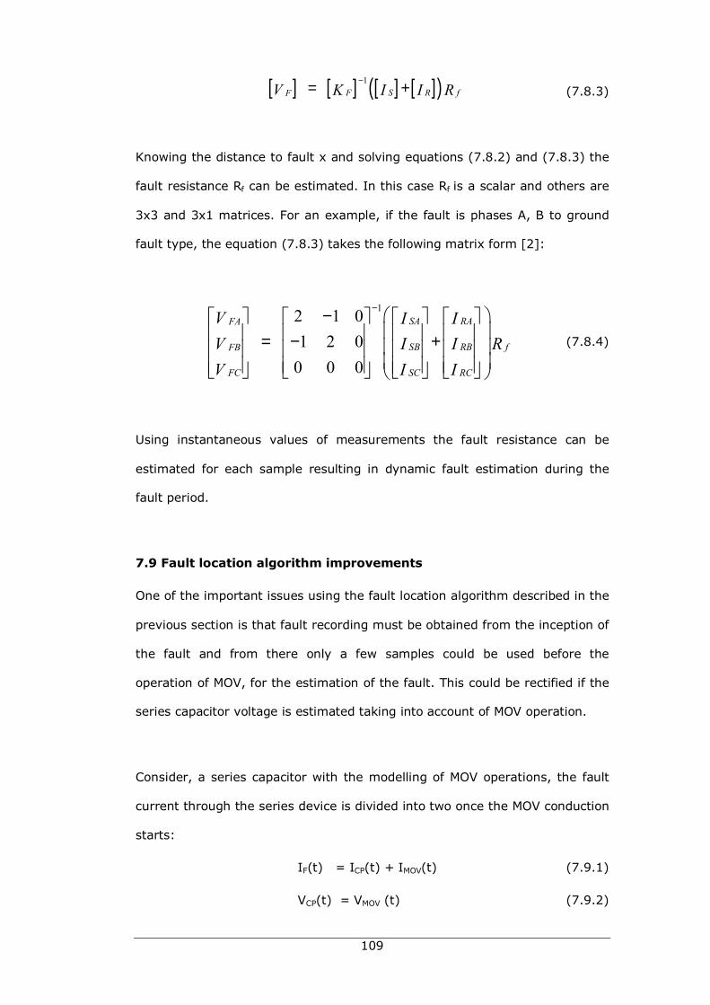
109
(7.8.3)
Knowing the distance to fault x and solving equations (7.8.2) and (7.8.3) the
fault resistance Rf can be estimated. In this case Rf is a scalar and others are
3x3 and 3x1 matrices. For an example, if the fault is phases A, B to ground
fault type, the equation (7.8.3) takes the following matrix form [2]:
(7.8.4)
Using instantaneous values of measurements the fault resistance can be
estimated for each sample resulting in dynamic fault estimation during the
fault period.
7.9 Fault location algorithm improvements
One of the important issues using the fault location algorithm described in the
previous section is that fault recording must be obtained from the inception of
the fault and from there only a few samples could be used before the
operation of MOV, for the estimation of the fault. This could be rectified if the
series capacitor voltage is estimated taking into account of MOV operation.
Consider, a series capacitor with the modelling of MOV operations, the fault
current through the series device is divided into two once the MOV conduction
starts:
IF(t) = ICP(t) + IMOV(t) (7.9.1)
VCP(t) = VMOV (t) (7.9.2)
[ ] [ ] [ ] [ ]( )1S R fFFV I I RK
−= +
12 1 01 2 0
0 0 0
SA RAFA
SB RB fFB
SC RCFC
V I IV I I RV I I
−− = − +
110
Substituting VMOV (t) with VCP(t) an expression can be obtained for the total
instantaneous fault current IF(t) in terms of VCP(t) as described in chapter 6
equation (6.8.9). However, equation (6.8.9) is a recursive type discrete
expression and it requires initial conditions for starting the recursive process
[10, 14].
To solve this problem, consider the operating conditions of the series
compensation device with respect to the rising of instantaneous fault current
during a fault cycle as shown in Fig 7.9.1.
Fig 7.9.1 Operating cycle of the series compensation device
If the fault current is traced back to the time steps before the fault occurred,
the voltage drop across the capacitor is purely capacitive and MOV branch is
open circuited and has no effect on the voltage drop. If the value of the
capacitor and the through current are known the initial voltage drop can be
computed using phasor equation for the capacitor [10, 14].
0 0.01 0.02 0.03 0.04 0.05 0.06 0.07-4
-3
-2
-1
0
1
2
3
4x 10
5
TIME (Sec.)
VO
LTS
, A
CapacitorVoltage drop
Fault current
111
0 10 20 30 40 50 60-4
-3
-2
-1
0
1
2
3
4x 10
5
Time, ms
SC
U V
olta
ge D
rop(
in V
olt
s)
Comparision of SCU instantanious voltage drop Acutal Vs calculated
Fault Inception
Actual voltage drop
Calulated voltage drop
When the new improvement is added to the estimation of series capacitor
voltage drop, the actual voltage drop obtained from EMTP/ATP simulation
closely match with the estimated values as shown in Fig 7.9.2.
(a) (b)
Fig 7.9.2 Series capacitor voltage drop comparison (Actual Vs
Estimated)
7.10 Practical issues concerned with estimation of fault location
In implementation of this algorithm in a practical environment, there are
several major practical issues to be addressed and investigated for the effects
on accuracy of the fault location algorithm. The following sections describe
several major issues investigated and how the proposed modifications could
affect the accuracy of the fault location algorithm [10, 14].
7.10.1 Locating Fault with respect to SCU
The fault can occur anywhere on the transmission line and hence it is
important to know that the fault is before or after the series compensation
device, with respect to the sending end where the fault locator is installed.
1200 1220 1240 1260 1280 1300
3.5
4
4.5
5
5.5
x 104
Time steps
Vol
tage
dro
p
Actual voltage drop Calulated voltage drop
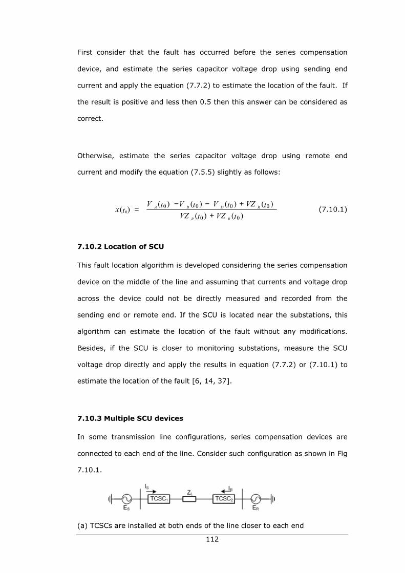
112
First consider that the fault has occurred before the series compensation
device, and estimate the series capacitor voltage drop using sending end
current and apply the equation (7.7.2) to estimate the location of the fault. If
the result is positive and less then 0.5 then this answer can be considered as
correct.
Otherwise, estimate the series capacitor voltage drop using remote end
current and modify the equation (7.5.5) slightly as follows:
(7.10.1)
7.10.2 Location of SCU
This fault location algorithm is developed considering the series compensation
device on the middle of the line and assuming that currents and voltage drop
across the device could not be directly measured and recorded from the
sending end or remote end. If the SCU is located near the substations, this
algorithm can estimate the location of the fault without any modifications.
Besides, if the SCU is closer to monitoring substations, measure the SCU
voltage drop directly and apply the results in equation (7.7.2) or (7.10.1) to
estimate the location of the fault [6, 14, 37].
7.10.3 Multiple SCU devices
In some transmission line configurations, series compensation devices are
connected to each end of the line. Consider such configuration as shown in Fig
7.10.1.
(a) TCSCs are installed at both ends of the line closer to each end
)()()()()()(
)(00
00000
tVZtVZtVZtVtVtV
txRR
RDBA
++−−
=
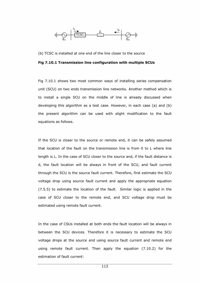
113
(b) TCSC is installed at one end of the line closer to the source
Fig 7.10.1 Transmission line configuration with multiple SCUs
Fig 7.10.1 shows two most common ways of installing series compensation
unit (SCU) on two ends transmission line networks. Another method which is
to install a single SCU on the middle of line is already discussed when
developing this algorithm as a test case. However, in each case (a) and (b)
the present algorithm can be used with slight modification to the fault
equations as follows.
If the SCU is closer to the source or remote end, it can be safely assumed
that location of the fault on the transmission line is from 0 to L where line
length is L. In the case of SCU closer to the source and, if the fault distance is
d, the fault location will be always in front of the SCU, and fault current
through the SCU is the source fault current. Therefore, first estimate the SCU
voltage drop using source fault current and apply the appropriate equation
(7.5.5) to estimate the location of the fault. Similar logic is applied in the
case of SCU closer to the remote end, and SCU voltage drop must be
estimated using remote fault current.
In the case of CSUs installed at both ends the fault location will be always in
between the SCU devices. Therefore it is necessary to estimate the SCU
voltage drops at the source end using source fault current and remote end
using remote fault current. Then apply the equation (7.10.2) for the
estimation of fault current:
114
(7.10.2)
where VD1 (t0) and VD2 (t0) are instantaneous voltage drops of SCU at source
and remote ends.
7.10.4 MOV spark gap protection
During a heavy fault current case, the MOV can be subjected to over heating
due to the energy dissipation in the MOV exceeding its limit. The thermal limit
of the MOV mainly depends on the level of through fault current and the
duration of conduction of the MOV. To safeguard the MOV from such a
condition, spark gap is provided to bypass the current until the fault level is
reduced to a reasonably safe level. The present fault location method needs
to be modified to handle such conditions during the estimation of fault
distance. [14]
However, the recent development of series compensation devices suggest
that some manufacturers have developed MOV devices that safely operate
without an air gap protection device [59]. In this case the present algorithm
does not need any modifications in order to accurately estimate fault location
using the preposed method. Others stated that thyristor valves can be
operated in parallel with the MOV to protect it from overheating [59].
To conclude this investigation, an improvement to this algorithm can be made
by considering the operation of simple air gap. Since the characteristics of
the air gap is known from the manufacturer, limiting fault current and
duration can be detected during the fault estimation. Using this condition,
over these limits, capacitor voltage drop VD can be approximated to zero. First
we compare the level of fault current with MOV over heating limit and its
1 20
0 0 0 0 0
0 0
( ) ( ) ( ) ( ) ( )( )( ) ( )
A B D D R
R R
V V V V VZt t t t tx tVZ VZt t
− − + +=
+

115
duration; fault location can then be estimated using equation (7.5.5) with VD
≈ 0.
7.10.5 Data synchronising error
Since this algorithm is developed using measurements of fault signal from
both ends of the line, data must be accurately synchronized for the estimation
of fault location. The synchronisation of signals over several hundred of
kilometers is not a difficult task considering the emerging telecommunication
technology, such as low cost high precision intelligent types of digital fault
recorders which can be setup several thousand kilometers apart with the help
of GPS receivers, as illustrated in Fig. 3.7.1.
The GPS system consists of many satellites, which were launched by the
United State for defense requirements and readily available for other
commercial purposes through out the world. Each satellite has a highly
accurate atomic clock on board for sending signals to earth giving accurate
time reference for the signals. The accuracy of timing of these reference
signals are in the range of a few nanoseconds and are more than capable of
synchronising high frequency signals. A research conduct on testing of
transmission line tele-protection schemes using GPS system shows that
accuracy of synchronisation of local and remote fault signals can be obtained
up to 1µs [59].
However, the present algorithm was tested introducing local and remote ends
data synchronisation error up to 0.1 ms and it was observed that the average
fault location error is still within ± 0.1% of the results obtained under normal
case.
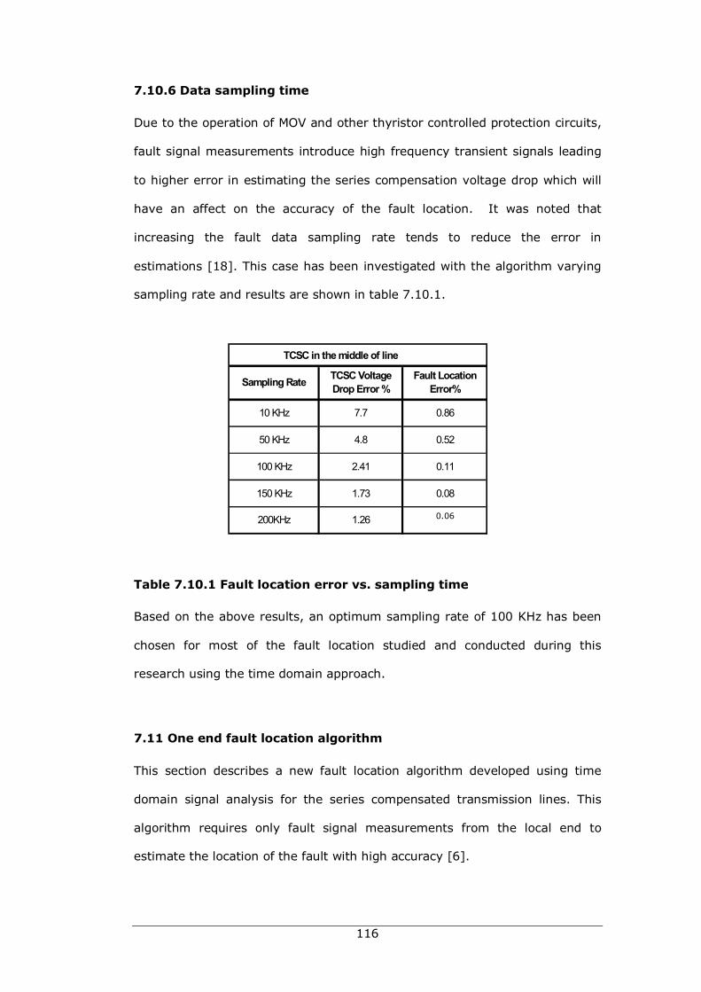
116
7.10.6 Data sampling time
Due to the operation of MOV and other thyristor controlled protection circuits,
fault signal measurements introduce high frequency transient signals leading
to higher error in estimating the series compensation voltage drop which will
have an affect on the accuracy of the fault location. It was noted that
increasing the fault data sampling rate tends to reduce the error in
estimations [18]. This case has been investigated with the algorithm varying
sampling rate and results are shown in table 7.10.1.
Table 7.10.1 Fault location error vs. sampling time
Based on the above results, an optimum sampling rate of 100 KHz has been
chosen for most of the fault location studied and conducted during this
research using the time domain approach.
7.11 One end fault location algorithm
This section describes a new fault location algorithm developed using time
domain signal analysis for the series compensated transmission lines. This
algorithm requires only fault signal measurements from the local end to
estimate the location of the fault with high accuracy [6].
TCSC in the middle of line
150 KHz 1.73 0.08
200KHz 1.26 0.61
50 KHz 4.8 0.52
100 KHz 2.41 0.11
Sampling Rate TCSC Voltage Drop Error %
Fault Location Error%
10 KHz 7.7 0.86
0.06
117
As previously explained, the estimation of series capacitor voltage drop is the
key to the accuracy of the fault location using this algorithm and the method
implemented in two ends algorithm could be used for the same purpose.
Consider a transmission line system which is similar to the one used in two
ends algorithm as shown in Fig 7.3.1. The fault locator is installed at the
sending end of the two ends transmission network. It is assumed that the
series compensation unit is located at the centre of the line. Consider a two
phase to earth solid fault after the SCU installation and faulty signals are
measured from the sending end only.
7.12 Development of One end algorithm
If the distance to the fault from the sending end is x and fault voltage during
the fault is VG, fault equation from the sending end can be obtained in the
form:
7.12.1
where VS and IS are sending end voltage and current during the fault. ZL is
the total line impedance and VD refers to the capacitor voltage drop and all
measurements are instantaneous values referenced to a given time [38].
Since the transmission network with three phases, equation (7.12.1) can be
expanded in matrix form:
7.12.2
where phases are identified as A, B and C. Line impedance is written in 3x3
matrix referring to self and mutual impedances s and m subscripts. If the
solid fault is on phase A and B, it is reasonable to assume that instantaneous
fault voltage at phase A and B are approximately identical [6]. Therefore, an
[ ] [ ] [ ] [ ] [ ]VVIV GDSsZLx =−−
=
−
−
VVV
VVV
III
ZZZZZZZZZ
VVV
GC
GB
GA
DC
DB
DA
SC
SB
SA
SCCMCBMCA
MBCSBBMBA
MACMABSAA
SC
SB
SA
x
118
expression for distance to fault x can be obtained directly using this equality
and it takes the following form:
7.12.3
For a completely transposed line, self and mutual inductance of each phase is
approximately identical. And also load current in phase C compared to fault
current in phases A and B can be considered small and assumed as zero. Now
equation (7.12.3) can be further simplified:
7.12.4
In this case three phase voltages and three phase fault currents through the
SCU is measured and recorded at the sending end at a sampling rate of
100KHz. Considering the equation (7.12.4) all the terms on the left is
estimated using equations described in section 7.3 and 7.4. At any give time
t during the fault, fault distance x(t) can be written:
(7.12.5)
If the fault has occurred on the left of the series compensation unit, the fault
equation becomes further simpler due to the absence of SCU for the fault
current from the sending side. Selection of an occurring fault on the left or
right of SCU can be determined using a similar argument described in section
7.10.1 [6].
( ) ( ) ( )SA SB DA DB
SAA MBA SA SBB SB MBC SCMBA MAC
VV V VxZ ZZ Z I Z I Z I
− − +=
+ +− −−
( ) ( )SA SB DA DB
S M SA S SBM
VV V VxZZ Z I Z I
− − +=
+ −−
( ) ( )( ) ( ) ( ) ( )
( )( ) ( )
SA SB DA DB
S M SA S SBM
t t t tVV V Vx tt tZZ Z I Z I
− − +=
+ −−
119
One of the drawbacks of this fault location algorithm is that the type of fault
must be known precisely and what phases are at fault. Identifying fault types
using measured fault signals are explained in many different ways in other
research works and will not be discussed in this research document [60].
Present algorithm cannot be directly applied, if the fault involves being only in
one phase (P-E fault). One way to overcome this problem is to apply two
stages with primarily estimating the fault location using phasor based
approach and apply this method to refine the results to estimate the distance
to the fault more accurately [6].
7.13 Implementations of the algorithm
A two port transmission network similar to the one described in section 7.3 is
implemented using power system modelling software using EMTP/ATP
software with the SCU is located in the middle of the line.
Line voltages and currents from one end is monitored and recorded during the
simulation of faults before and after the location of SCU. The fault signals are
recorded with the sampling rate of 100 KHz similar to previous fault location
algorithm for various types of faults involving more that one phase. The
comparison of results of algorithms developed in this research work with
other algorithms developed by many authors and are analysed in chapter 8.
7.14 Algorithm improvement for time varying fault resistance
One end fault location algorithm described in the previous section is further
tested for time varying fault resistance modelled using EMTP/ATP software.
During the simulation, fault resistance is changed from 10 to 6.5 ohms in
three steps implementing type 97 staircase time varying resistance R(t)
described in page 5F-1 of the ATP rule book [11]. A typical dynamic
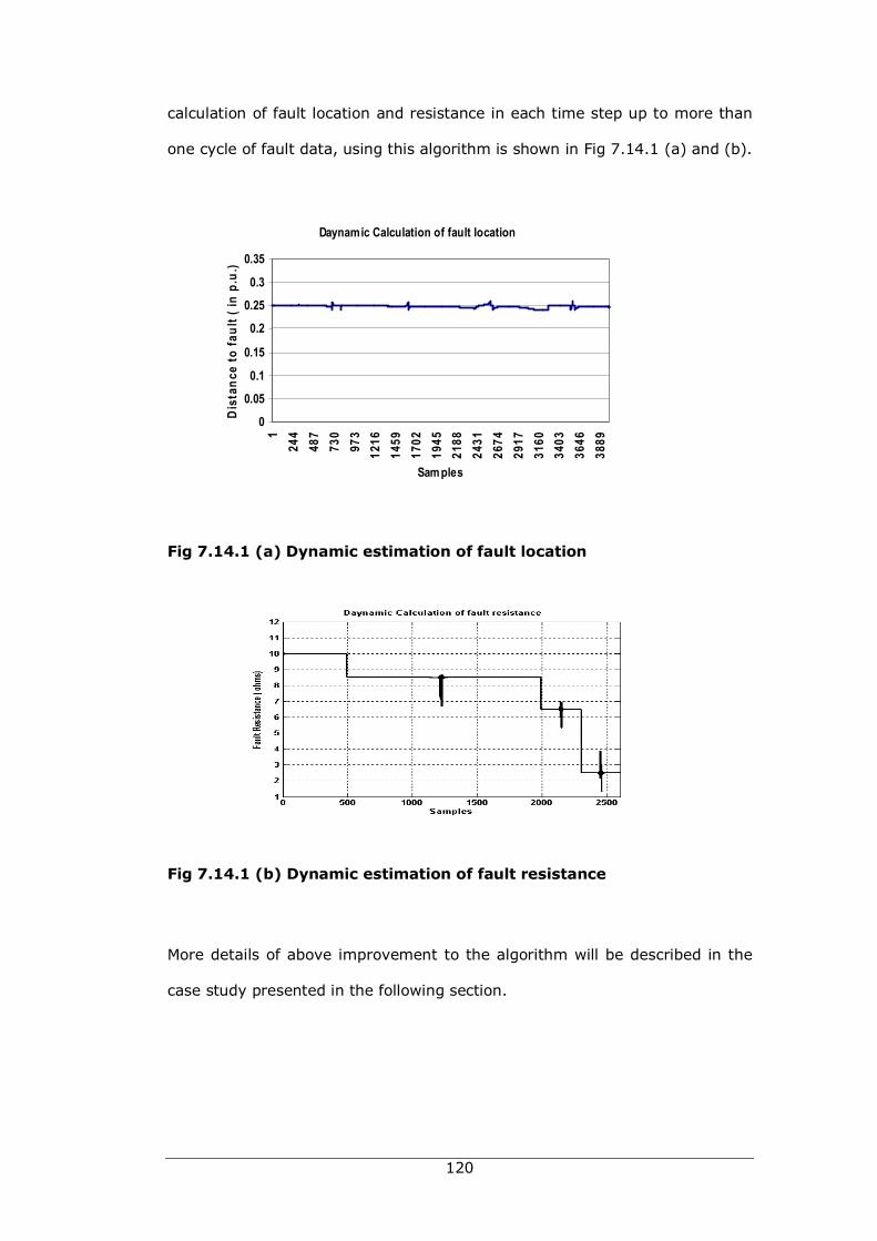
120
calculation of fault location and resistance in each time step up to more than
one cycle of fault data, using this algorithm is shown in Fig 7.14.1 (a) and (b).
Fig 7.14.1 (a) Dynamic estimation of fault location
Fig 7.14.1 (b) Dynamic estimation of fault resistance
More details of above improvement to the algorithm will be described in the
case study presented in the following section.
Daynamic Calculation of fault location
0
0.05
0.1
0.15
0.2
0.25
0.3
0.351
244
487
730
973
1216
1459
1702
1945
2188
2431
2674
2917
3160
3403
3646
3889
Samples
Dis
tanc
e to
faul
t ( in
p.u
.)
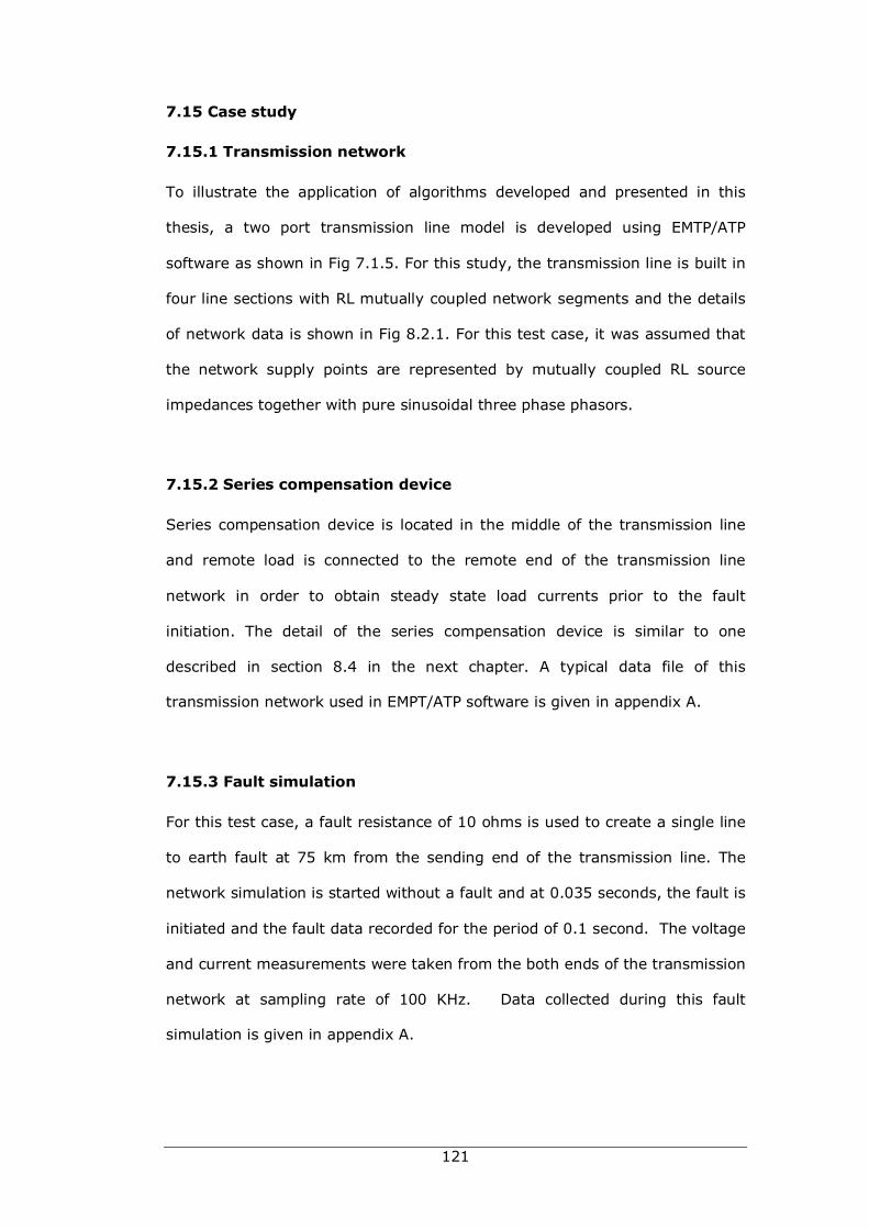
121
7.15 Case study
7.15.1 Transmission network
To illustrate the application of algorithms developed and presented in this
thesis, a two port transmission line model is developed using EMTP/ATP
software as shown in Fig 7.1.5. For this study, the transmission line is built in
four line sections with RL mutually coupled network segments and the details
of network data is shown in Fig 8.2.1. For this test case, it was assumed that
the network supply points are represented by mutually coupled RL source
impedances together with pure sinusoidal three phase phasors.
7.15.2 Series compensation device
Series compensation device is located in the middle of the transmission line
and remote load is connected to the remote end of the transmission line
network in order to obtain steady state load currents prior to the fault
initiation. The detail of the series compensation device is similar to one
described in section 8.4 in the next chapter. A typical data file of this
transmission network used in EMPT/ATP software is given in appendix A.
7.15.3 Fault simulation
For this test case, a fault resistance of 10 ohms is used to create a single line
to earth fault at 75 km from the sending end of the transmission line. The
network simulation is started without a fault and at 0.035 seconds, the fault is
initiated and the fault data recorded for the period of 0.1 second. The voltage
and current measurements were taken from the both ends of the transmission
network at sampling rate of 100 KHz. Data collected during this fault
simulation is given in appendix A.
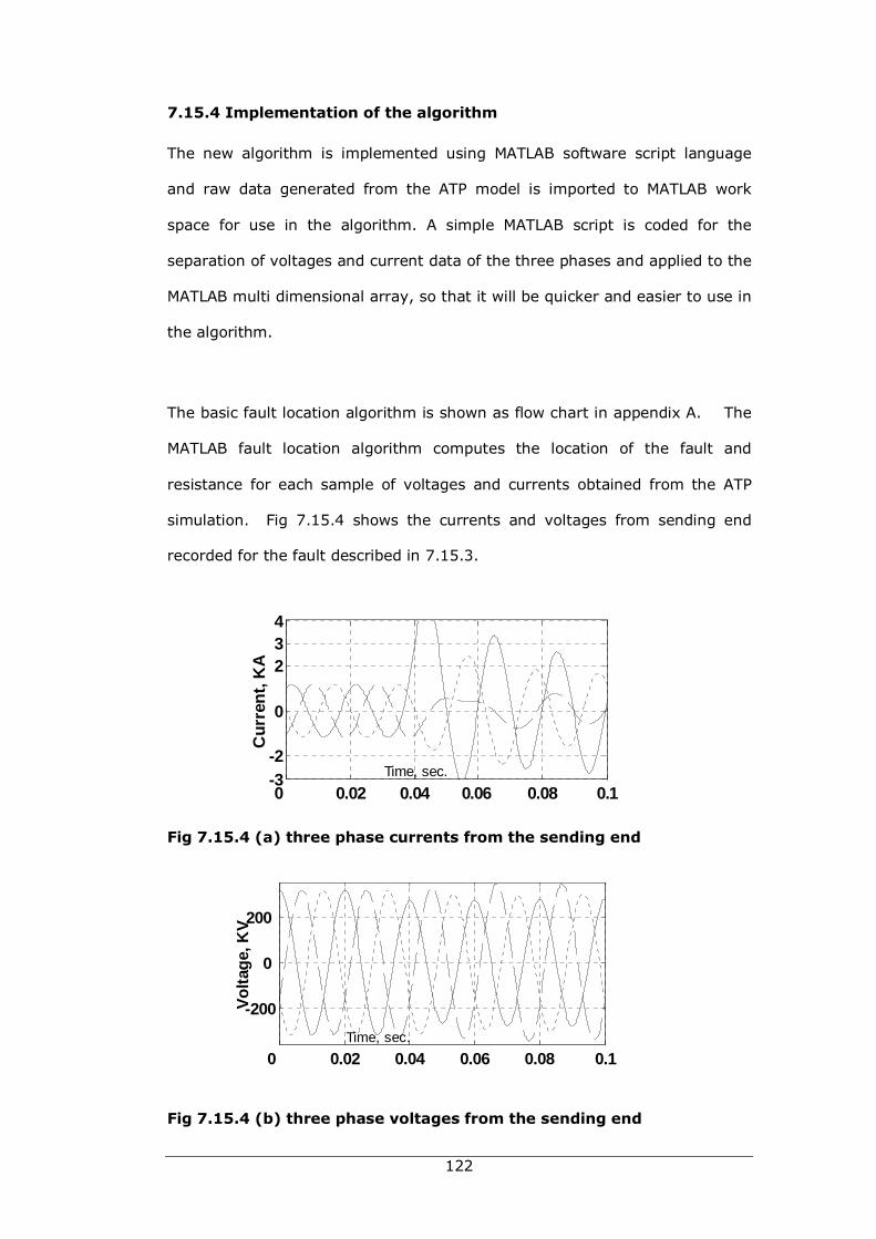
122
7.15.4 Implementation of the algorithm
The new algorithm is implemented using MATLAB software script language
and raw data generated from the ATP model is imported to MATLAB work
space for use in the algorithm. A simple MATLAB script is coded for the
separation of voltages and current data of the three phases and applied to the
MATLAB multi dimensional array, so that it will be quicker and easier to use in
the algorithm.
The basic fault location algorithm is shown as flow chart in appendix A. The
MATLAB fault location algorithm computes the location of the fault and
resistance for each sample of voltages and currents obtained from the ATP
simulation. Fig 7.15.4 shows the currents and voltages from sending end
recorded for the fault described in 7.15.3.
Fig 7.15.4 (a) three phase currents from the sending end
Fig 7.15.4 (b) three phase voltages from the sending end
0 0.02 0.04 0.06 0.08 0.1-3-2
0
234
Cur
ren
t, K
A
Time, sec.
0 0.02 0.04 0.06 0.08 0.1
-200
0
200
Vo
ltag
e, K
V
Time, sec.
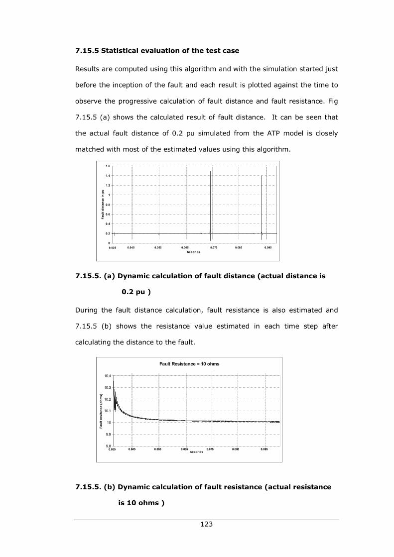
123
7.15.5 Statistical evaluation of the test case
Results are computed using this algorithm and with the simulation started just
before the inception of the fault and each result is plotted against the time to
observe the progressive calculation of fault distance and fault resistance. Fig
7.15.5 (a) shows the calculated result of fault distance. It can be seen that
the actual fault distance of 0.2 pu simulated from the ATP model is closely
matched with most of the estimated values using this algorithm.
7.15.5. (a) Dynamic calculation of fault distance (actual distance is
0.2 pu )
During the fault distance calculation, fault resistance is also estimated and
7.15.5 (b) shows the resistance value estimated in each time step after
calculating the distance to the fault.
7.15.5. (b) Dynamic calculation of fault resistance (actual resistance
is 10 ohms )
0
0.2
0.4
0.6
0.8
1
1.2
1.4
1.6
Seconds
Faul
t dis
tanc
e in
pu
0.035 0.045 0.055 0.065 0.075 0.085 0.095
Fault Resistance = 10 ohms
9.8
9.9
10
10.1
10.2
10.3
10.4
seconds
Faul
t res
itanc
e (o
hms)
0.075 0.085 0.0950.035 0.045 0.055 0.065
124
In each case, a number of results calculated using the algorithm is more than
3000 and hence it is difficult to give in table format. However, the result
samples are statistically analysed and given in table 7.15.1. The accuracy of
the results in this test case is 99.8 % for the fault distance and 99.1% for the
fault resistance. Fault location error can be further minimised by applying a
simple filter to the row result array in order to remove very few instantaneous
high and low values before applying the statistical analysis.
Table 7.15.1 Statistical results of test case
7.16 Performance evaluation and comparison of results
In order to evaluate the accuracy and robustness of the fault location
algorithm, over 90 cases of fault simulations were conducted with varying
fault type using EMTP/ATP software and applying fault data to estimate the
average, maximum and minimum fault location error [14]. The variations
applied to generate more fault cases in this evaluation are explained in detail
in chapter 8.
In addition, results obtained from this algorithm and other algorithms
developed in this thesis are compared with each other, focusing on the
accuracy of the fault location and further comparisons have been conducted
with fault location algorithms preposed by other authors [2, 15]. These
details are given in chapter 8.
Actual fault distance = 0.2 pu and fault resistance = 10 ohms
Result samples = 3195Fault Distance
(pu)Fault Resistance
(ohm)
Mean value 0.1996 10.092
Result Varience 0.0312 0.0196
STD Deviation 0.001 0.0002
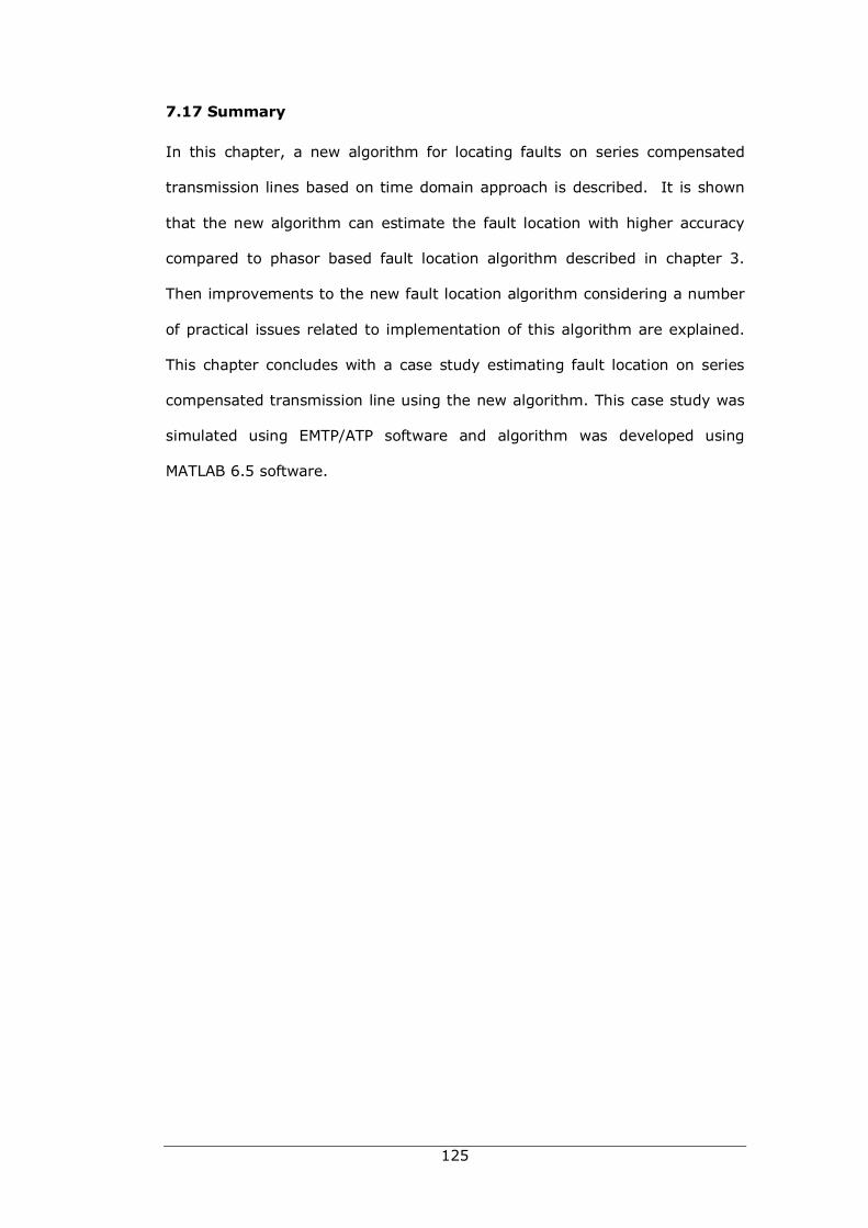
125
7.17 Summary
In this chapter, a new algorithm for locating faults on series compensated
transmission lines based on time domain approach is described. It is shown
that the new algorithm can estimate the fault location with higher accuracy
compared to phasor based fault location algorithm described in chapter 3.
Then improvements to the new fault location algorithm considering a number
of practical issues related to implementation of this algorithm are explained.
This chapter concludes with a case study estimating fault location on series
compensated transmission line using the new algorithm. This case study was
simulated using EMTP/ATP software and algorithm was developed using
MATLAB 6.5 software.
126
Chapter 8.0
Assessment and comparison of fault
location under varies fault conditions
8.1 Introduction
Several fault location algorithms developed in this research work for series
compensated transmission lines have been described in Chapters 3 and 7.
Further, the algorithms have been implemented in MATLAB environments for
testing the accuracy of fault estimation. Fault data required for the testing of
algorithms are obtained from the simulation of a two port transmission line
network with the insertion of a series compensation device in the middle of
the line. The transmission line model developments and fault simulations are
conducted using a MATLAB Power system Block set tool. Towards the end of
this research work, more accurate and advanced transmission line models
were created and simulated with very well proven EMTP/ATP software. Such
models and simulations both have become very popular among power system
research groups all over the world [38, 58, 61, 62].
This chapter discusses the details of specific transmission line models and
other power system components, which have been used for the simulation of
faults in relation to each fault location algorithm. During this research work,
each fault location algorithm have been tested using a wide range of fault
cases simulated by the MATLAB and EMTP/ATP software, and statistical results
127
have been published by the author and co-workers in many conferences and
journal papers [1, 6, 10, 14, 16, 18, 19, 37, 39, 56, 57].
The statistical results obtained from the new algorithm developed using
phasor based and time domain approaches during this research [1] is
compared with the results from other authors and are given in section 8.12
[2, 63]
8.2 Transmission line configurations
To evaluate the accuracy of fault location algorithms described in the previous
chapters, the modelling of transmission line system is required to be precise
and very close to the real power system. Most of the case studies shown in
this research work are based on two ends transmission line with supplies
connected to each end, with the initial load on the remote end prior to the
fault initiation. A typical two ends transmission line model used for the testing
of fault location algorithms is shown in Fig 8.2.1. For the basic test cases, the
series compensation device is placed in the middle of the line considering
direct measurements of the SCU voltages are not available at the line ends.
Fig 8.2.1 Two ends transmission line model
The series compensation level is started with 50% for basic test cases and
varied ± 20% for obtaining statistical results with many other parameter
(1-x)ZL
MOV
C
VF
F2
IF
F1
Station R
ES
Station S
ZS xZL
IS
VS
FLZR
ER
IR
VR
GPSReceiver
DFR
GPSReceiver
DFRCoomunication lines
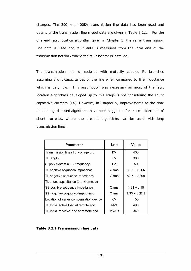
128
changes. The 300 km, 400KV transmission line data has been used and
details of the transmission line model data are given in Table 8.2.1. For the
one end fault location algorithm given in Chapter 3, the same transmission
line data is used and fault data is measured from the local end of the
transmission network where the fault locator is installed.
The transmission line is modelled with mutually coupled RL branches
assuming shunt capacitances of the line when compared to line inductance
which is very low. This assumption was necessary as most of the fault
location algorithms developed up to this stage is not considering the shunt
capacitive currents [14]. However, in Chapter 9, improvements to the time
domain signal based algorithms have been suggested for the consideration of
shunt currents, where the present algorithms can be used with long
transmission lines.
Table 8.2.1 Transmission line data
Parameter Unit Value
Transmission line (TL) voltage L-L KV 400
TL length KM 300
Supply system (SS) frequency HZ 50
TL positive sequence impedance Ohms 8.25 + j 94.5
TL negative sequence impedance Ohms 82.5 + J 308
TL shunt capacitance (per kilometre)
SS positive sequence impedance Ohms 1.31 + J 15
SS negative sequence impedance Ohms 2.33 + J 26.8
Location of series compensation device KM 150
TL Initial active load at remote end MW 400
TL Initial reactive load at remote end MVAR 340

129
For the simplicity, although it not required, the transmission line is assumed
to be uniformly transposed where line impedance of the model can be
simplified as:
where self inductance of each phase is identical and mutual effects between
lines are also considered similar values [1].
8.3 Supply systems
The supply system at each end consists of ideal sinusoidal voltage source with
the peak value of Vm could be calculated as follows:
Line to line voltage = 400 KV
Phase voltage = 230.94 KV
Then the peak value = √2 * 230.94 = 326599 volts
The source impedances are considered identical at each source and mutually
coupled LR series branch have been added to represent the internal source
impedances of the supply systems [2].
8.4 Series compensation device
The series compensation device installed on the transmission line model has
the following components:
Series capacitor branch : Used in all fault location algorithms
MOV branch : Used in all fault location algorithms
Spark gap branch : Used only in fault location algorithms developed
based on time domain analysis
LS Lm Lm
Lm LS Lm
Lm Lm LS
Z Z ZZ Z ZZ Z Z
130
Thyristor valve branch : Improved version of above algorithm for TCSE
series device
If the series compensation level is known and held constant throughout the
fault simulation, the value of the series capacitor can be calculated as follows:
Total line positive reactance = 94.5 ohms
Assume the required compensation level = 60%
Then the required capacitive reactance = 0.6 * 94.5=56.7 ohms
The value of the series capacitor = 1/ (2 * ∏ * 50 * 56.7)
= 56.14 µF
The series capacitor over voltage protection level for the implementation of
MOV device is computed in the following sequence:
The rated line voltage = 400 KV
The rated phase voltage = 400 /√3= 230.94 KV
Assume capacitor over voltage protection level is 2.5 time the rated.
The line current produces nominal capacitor voltage = 1.2 KA
The Capacitor protection level = 2.5 * 1.2KA * 56.7 * (2) 1/2
= 240.6 KV
The Capacitor protection level (instantaneous value) = 340.8 KV
Table 8.4.2 shows the basic data used for the modelling of series
compensation device with typical simulation details.
131
Table 8.4.1 Basic series compensation device data
However, values shown above are only typical, and some data have been
changed to generate different faulty cases, as required for the statistical
results of fault location estimates.
8.5 Remote end load
Steady state pre-fault power of the transmission network is modelled in the
fault simulation using LRC shunt impedance connected to the remote end of
the network. The values of the LRC components are calculated in order to
provide power flow of 300MW and -200MVAR in the direction of local to
remote ends [10, 39].
8.6 Fault model
A three phase fault model is created in the power network simulation
environment, using shunt LR branches connected to the faulted point and
ground via switches to control the fault switching during the simulation. This
model is capable of creating many types of faults with varying fault resistance
to simulate many fault conditions in transmission network at the desired
location. A typical switching arrangement for the three phase fault model is
shown in Fig 3.4.1.
Parameter Unit Value
Degree of compensation % 60 to 90
Reference current (r.m.s.) KA 4.4
Reference votlage (peak value) KV 340
Exponent - -23
Number of columns - 2
Spark gap (SP) - YES
SP operating level KJ 34.5
132
8.7 Fault simulation
During the start of the fault simulation, the fault is switched off and the
network set to carry the usual load currents according to the remote load.
Then fault switches are connected to the ground after 0.035 – 0.04 seconds
and stay connected during the rest of the simulation. The total time of the
simulation is in the range of 0.1 to 0.2 seconds and sampling time of fault
data recording is changed from 10 KHz to over 100 KHz. A typical fault
simulation data used during the EMTP/ATP simulation is given in table 8.7.1
[18].
Table 8.7.1 EMTP/ATP Fault simulation data
In MATLAB, data in Table 8.2.1 and 8.4.1 is loaded to the transmission line
model developed using power system block set components, running a
“LoadVaribles” subroutine coded in MATLAB script language prior to the
starting of the simulation process. These codes included the creation of a fault
and setting of the fault type and behaviour information. These settings were
updated manually for each simulated fault case.
Parameter Unit Value
Simulation method -
Total simulation time S 0.1
Sampling frequency KHz 100
Fault intiation time S 0.04
Fault resistance Ohms 1 to 10
Fault resistance varying steps - 4
Fault resistance varying Ohms 2.5 to 10
133
When the data loading is completed, the fault simulation is started
immediately and the measurement of data of three phase voltages and
currents from both ends of the transmission line is collected in the MATLAB
workspace, for the next stage where the fault location is estimated using the
new algorithm. A typical MATLAB fault simulation results in a three phase to
earth with fault resistance of 1 ohm is shown in Fig 8.7.1
Fig 8.7.1 Voltages and currents from Sending end
Fig 8.7.2 Voltages and currents from remote end
The details of the MATLAB fault simulation is described in Chapter 3 under
development of fault location algorithm using the phasor based approach [1].
In the next sections the simulation of the network fault using more accurate
EMTP/ATP software is described in detail.
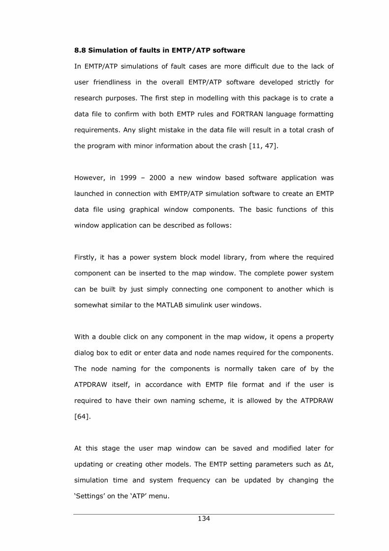
134
8.8 Simulation of faults in EMTP/ATP software
In EMTP/ATP simulations of fault cases are more difficult due to the lack of
user friendliness in the overall EMTP/ATP software developed strictly for
research purposes. The first step in modelling with this package is to crate a
data file to confirm with both EMTP rules and FORTRAN language formatting
requirements. Any slight mistake in the data file will result in a total crash of
the program with minor information about the crash [11, 47].
However, in 1999 – 2000 a new window based software application was
launched in connection with EMTP/ATP simulation software to create an EMTP
data file using graphical window components. The basic functions of this
window application can be described as follows:
Firstly, it has a power system block model library, from where the required
component can be inserted to the map window. The complete power system
can be built by just simply connecting one component to another which is
somewhat similar to the MATLAB simulink user windows.
With a double click on any component in the map widow, it opens a property
dialog box to edit or enter data and node names required for the components.
The node naming for the components is normally taken care of by the
ATPDRAW itself, in accordance with EMTP file format and if the user is
required to have their own naming scheme, it is allowed by the ATPDRAW
[64].
At this stage the user map window can be saved and modified later for
updating or creating other models. The EMTP setting parameters such as ∆t,
simulation time and system frequency can be updated by changing the
‘Settings’ on the ‘ATP’ menu.
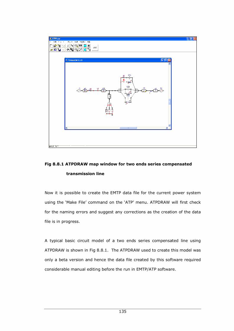
135
Fig 8.8.1 ATPDRAW map window for two ends series compensated
transmission line
Now it is possible to create the EMTP data file for the current power system
using the ‘Make File’ command on the ‘ATP’ menu. ATPDRAW will first check
for the naming errors and suggest any corrections as the creation of the data
file is in progress.
A typical basic circuit model of a two ends series compensated line using
ATPDRAW is shown in Fig 8.8.1. The ATPDRAW used to create this model was
only a beta version and hence the data file created by this software required
considerable manual editing before the run in EMTP/ATP software.
136
From the ATP menu this data file can be run in many ways to create
EMTP/ATP output files, and additional details of EMTP simulation and other
facilities can be found on the ATPDRAW help file [64].
8.9 Measurement of fault data
During the simulation, fault data from the transmission line ends are
monitored and recorded with suitable time tags to use in the estimation of the
fault location. In most of the fault simulation studies the ATP model includes
both capacitive voltage transformers and current transformers. In addition an
anti-aliasing filter has been used to reduce the effects of high frequency
signals present during the fault simulation.
8.10 Processing of fault data
The fault data measured from the EMTP/ATP simulation is stored in EMTP plot
file binary format with the file extension of PL4 not being directly used in any
other application software, such as MS products or a MATLAB package.
However in 2001, the Bonneville Power Administration introduced a software
product called an ATP Analyzer to process signals in the PL4 format and the
following section briefly describes the application of this software [65].
8.10.1 ATP analyzer
This application is window based and it has many features that can be used to
read and analyse fault signals in Pl4 binary format. Fig 8.10.1 shows the main
window of the ATP analyser, after opening an ATP output file after simulating
a data case 123/36.

137
Fig 8.10.1 ATP analyzer main windows
It has the main window and the sub window for manipulating ATP output files.
The main window has most of the menus which can import, open and analyse
PL4 output files. Using the file/new command any Pl4 file can be imported to
the sub window as a MS Access database. In the right pane of the sub window
it shows the listing of each signal recorded in the ATP output file. The main
advantage of this product is that binary signals can be directly saved as mdb
file and can be used virtually with any MS product for further processing or
presentations [65].
This product also has broad capabilities to process data signals and which can
be viewed as charts including the newly created data from the row signals.
More detail of this product is available in the product help file. After saving
the data as a MS Access database, it can be converted to MATLAB space via
MS Excel. However, other third party software is available nowadays to
convert PL4 files directly to MATLAB workspace. It was observed that using
one such product failed to create the MATLAB workspace stating that the file
was too large and conversion did not succeed [10].
138
8.11 Diversity of fault data
In order to evaluate the accuracy of the fault location developed during this
research work, numerous different fault cases have been generated using
MATLAB and EMTP/ATP simulation software and each fault case has been
played repeatedly in the developed fault algorithm to estimate the fault
location. The results obtained from the algorithm have been further processed
to compute the low, high and average fault location error maintaining the
classification of several groups as given below:
Main category: Fault type
Single phase to earth fault
Two phase to earth fault
Three phase to earth fault
Two phase fault
Three phase faults
Sub category: Fault resistance
I ohm fault resistance - fixed
10 ohms fault resistance – fixed
50 ohms fault resistance – fixed
10 ohms fault resistance – varying
50 ohms fault resistance – varying
Sub category: Fault Location (total line length is 300 km)
50 to 60 km from sending end
100 km from sending end
150 km from sending end
225 km from sending end
275 km from sending end
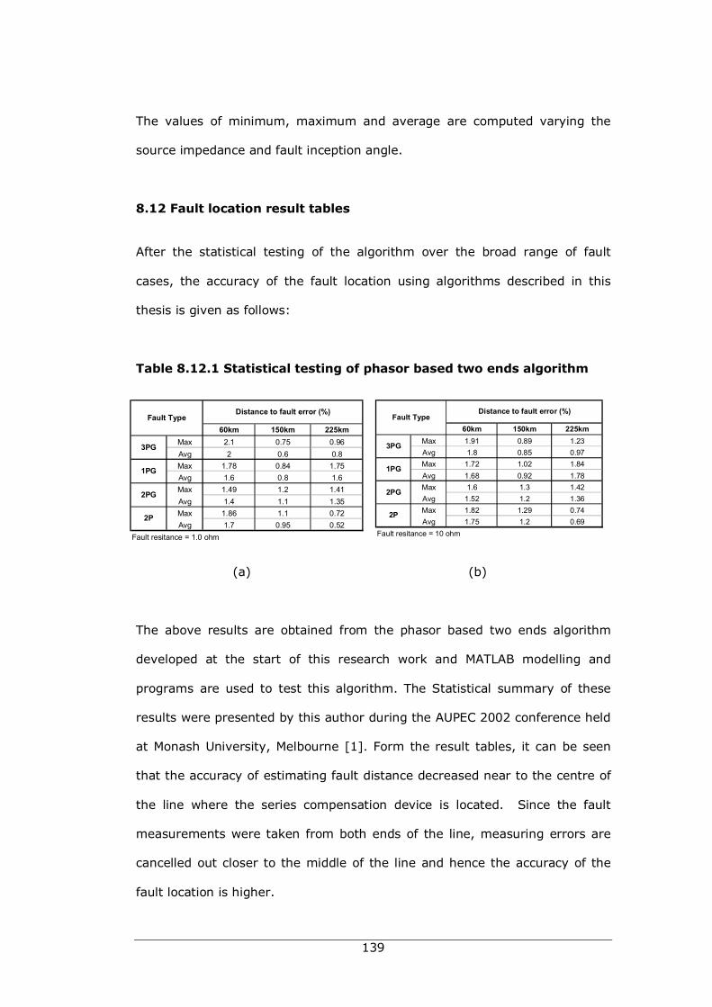
139
The values of minimum, maximum and average are computed varying the
source impedance and fault inception angle.
8.12 Fault location result tables
After the statistical testing of the algorithm over the broad range of fault
cases, the accuracy of the fault location using algorithms described in this
thesis is given as follows:
Table 8.12.1 Statistical testing of phasor based two ends algorithm
(a) (b)
The above results are obtained from the phasor based two ends algorithm
developed at the start of this research work and MATLAB modelling and
programs are used to test this algorithm. The Statistical summary of these
results were presented by this author during the AUPEC 2002 conference held
at Monash University, Melbourne [1]. Form the result tables, it can be seen
that the accuracy of estimating fault distance decreased near to the centre of
the line where the series compensation device is located. Since the fault
measurements were taken from both ends of the line, measuring errors are
cancelled out closer to the middle of the line and hence the accuracy of the
fault location is higher.
60km 150km 225kmMax 2.1 0.75 0.96Avg 2 0.6 0.8Max 1.78 0.84 1.75Avg 1.6 0.8 1.6Max 1.49 1.2 1.41Avg 1.4 1.1 1.35Max 1.86 1.1 0.72Avg 1.7 0.95 0.52
Fault resitance = 1.0 ohm
2P
Distance to fault error (%)
3PG
1PG
2PG
Fault Type60km 150km 225km
Max 1.91 0.89 1.23Avg 1.8 0.85 0.97Max 1.72 1.02 1.84Avg 1.68 0.92 1.78Max 1.6 1.3 1.42Avg 1.52 1.2 1.36Max 1.82 1.29 0.74Avg 1.75 1.2 0.69
Fault resitance = 10 ohm
1PG
2PG
2P
Fault TypeDistance to fault error (%)
3PG
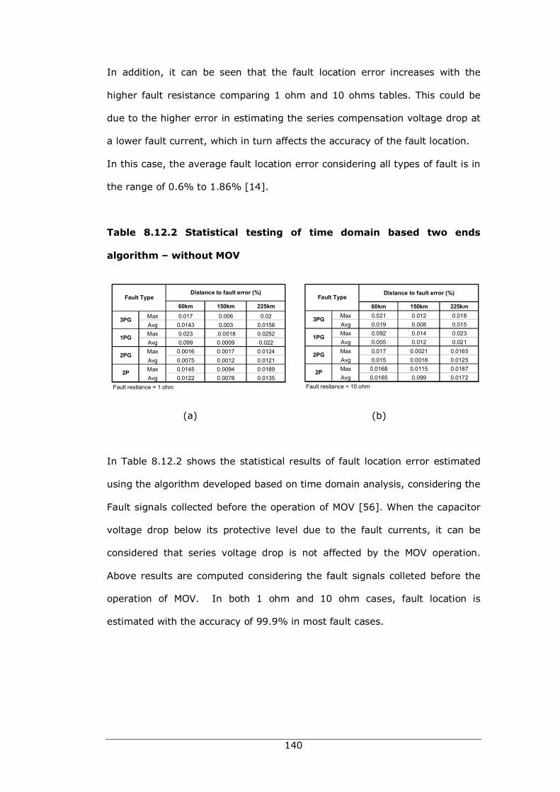
140
In addition, it can be seen that the fault location error increases with the
higher fault resistance comparing 1 ohm and 10 ohms tables. This could be
due to the higher error in estimating the series compensation voltage drop at
a lower fault current, which in turn affects the accuracy of the fault location.
In this case, the average fault location error considering all types of fault is in
the range of 0.6% to 1.86% [14].
Table 8.12.2 Statistical testing of time domain based two ends
algorithm – without MOV
(a) (b)
In Table 8.12.2 shows the statistical results of fault location error estimated
using the algorithm developed based on time domain analysis, considering the
Fault signals collected before the operation of MOV [56]. When the capacitor
voltage drop below its protective level due to the fault currents, it can be
considered that series voltage drop is not affected by the MOV operation.
Above results are computed considering the fault signals colleted before the
operation of MOV. In both 1 ohm and 10 ohm cases, fault location is
estimated with the accuracy of 99.9% in most fault cases.
60km 150km 225kmMax 0.017 0.006 0.02Avg 0.0143 0.003 0.0158Max 0.023 .0.0018 0.0252Avg 0.099 0.0009 0.022Max 0.0016 0.0017 0.0124Avg 0.0075 0.0012 0.0121Max 0.0145 0.0094 0.0189Avg 0.0122 0.0078 0.0135
Fault resitance = 1 ohm
2P
Fault TypeDistance to fault error (%)
3PG
1PG
2PG
60km 150km 225kmMax 0.021 0.012 0.018Avg 0.019 0.008 0.015Max 0.092 0.014 0.023Avg 0.005 0.012 0.021Max 0.017 0.0021 0.0165Avg 0.015 0.0018 0.0125Max 0.0168 0.0115 0.0187Avg 0.0165 0.099 0.0172
Fault resitance = 10 ohm
Distance to fault error (%)Fault Type
3PG
1PG
2PG
2P
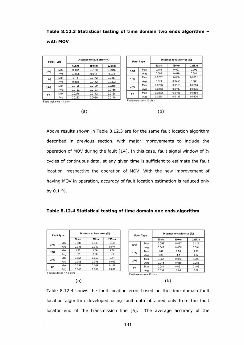
141
Table 8.12.3 Statistical testing of time domain two ends algorithm –
with MOV
(a) (b)
Above results shown in Table 8.12.3 are for the same fault location algorithm
described in previous section, with major improvements to include the
operation of MOV during the fault [14]. In this case, fault signal window of ¾
cycles of continuous data, at any given time is sufficient to estimate the fault
location irrespective the operation of MOV. With the new improvement of
having MOV in operation, accuracy of fault location estimation is reduced only
by 0.1 %.
Table 8.12.4 Statistical testing of time domain one ends algorithm
(a) (b)
Table 8.12.4 shows the fault location error based on the time domain fault
location algorithm developed using fault data obtained only from the fault
locator end of the transmission line [6]. The average accuracy of the
60km 150km 225kmMax 0.102 0.0168 0.0945Avg 0.0995 0.012 0.072Max 0.11 0.0172 0.0367Avg 0.108 0.0152 0.0302Max 0.0128 0.0109 0.0256Avg 0.0122 0.0103 0.0185Max 0.0276 0.0112 0.0168Avg 0.0222 0.0099 0.0178
Fault resitance = 1 ohm
Distance to fault error (%)
3PG
2PG
2P
Fault Type
1PG
60km 150km 225kmMax 0.105 0.023 0.092Avg 0.098 0.019 0.084Max 0.0752 0.068 0.0951Avg 0.071 0.0453 0.065Max 0.0256 0.0119 0.0213Avg 0.0253 0.0109 0.0195Max 0.0272 0.0166 0.0358Avg 0.0264 0.0133 0.0326
Fault resitance = 10 ohm
2PG
2P
Distance to fault error (%)Fault Type
3PG
1PG
60km 150km 225kmMax 0.039 0.045 0.08Avg 0.036 0.042 0.077Max 1.32 1.09 1.38Avg 1.2 0.96 1.3Max 0.051 0.059 0.14Avg 0.043 0.053 0.092Max 0.051 0.064 0.162Avg 0.042 0.059 0.097
Fault resitance = 1.0 ohm
2P
Distance to fault error (%)
3PG
1PG
2PG
Fault Type60km 150km 225km
Max 0.058 0.077 0.111Avg 0.047 0.068 0.094Max 1.42 1.24 1.18Avg 1.36 1.1 1.02Max 0.057 0.056 0.092Avg 0.048 0.055 0.086Max 0.041 0.061 0.106Avg 0.032 0.05 0.09
Fault resitance = 10 ohm
1PG
2PG
2P
Fault TypeDistance to fault error (%)
3PG
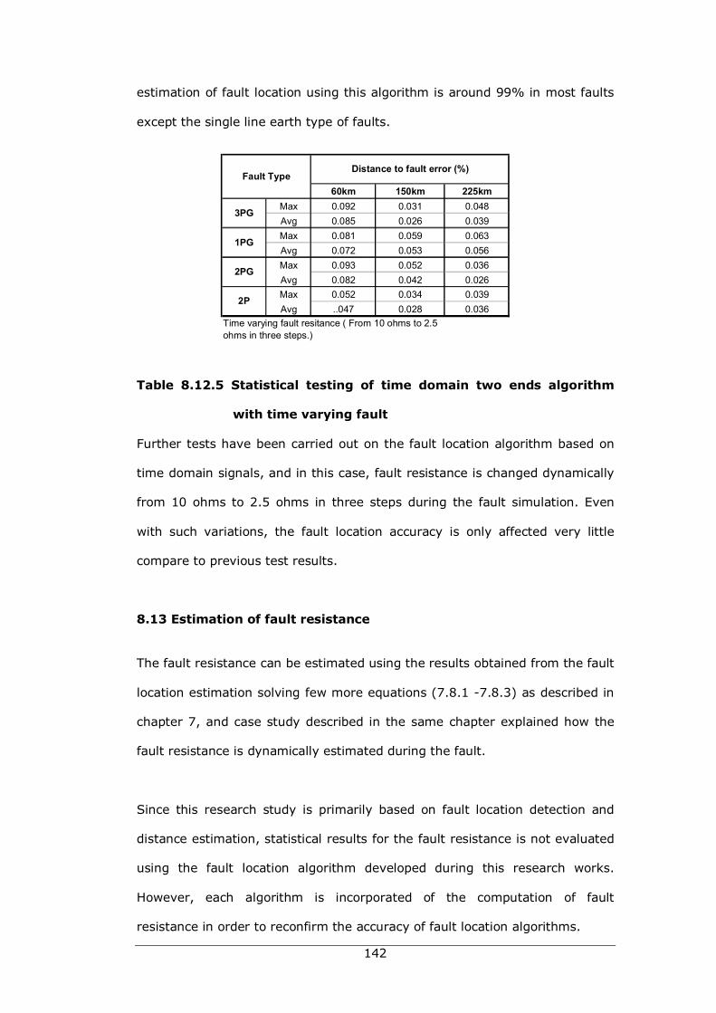
142
estimation of fault location using this algorithm is around 99% in most faults
except the single line earth type of faults.
Table 8.12.5 Statistical testing of time domain two ends algorithm
with time varying fault
Further tests have been carried out on the fault location algorithm based on
time domain signals, and in this case, fault resistance is changed dynamically
from 10 ohms to 2.5 ohms in three steps during the fault simulation. Even
with such variations, the fault location accuracy is only affected very little
compare to previous test results.
8.13 Estimation of fault resistance
The fault resistance can be estimated using the results obtained from the fault
location estimation solving few more equations (7.8.1 -7.8.3) as described in
chapter 7, and case study described in the same chapter explained how the
fault resistance is dynamically estimated during the fault.
Since this research study is primarily based on fault location detection and
distance estimation, statistical results for the fault resistance is not evaluated
using the fault location algorithm developed during this research works.
However, each algorithm is incorporated of the computation of fault
resistance in order to reconfirm the accuracy of fault location algorithms.
60km 150km 225kmMax 0.092 0.031 0.048Avg 0.085 0.026 0.039Max 0.081 0.059 0.063Avg 0.072 0.053 0.056Max 0.093 0.052 0.036Avg 0.082 0.042 0.026Max 0.052 0.034 0.039Avg ..047 0.028 0.036
2P
Time varying fault resitance ( From 10 ohms to 2.5 ohms in three steps.)
Distance to fault error (%)
3PG
1PG
2PG
Fault Type
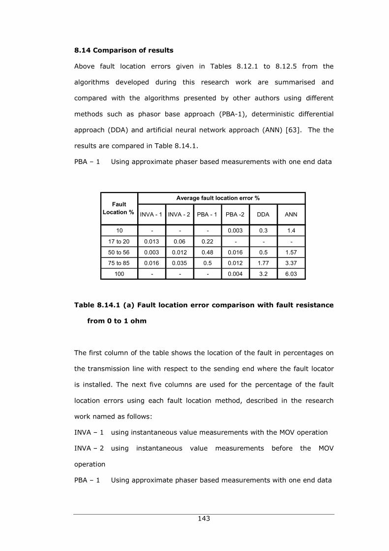
143
8.14 Comparison of results
Above fault location errors given in Tables 8.12.1 to 8.12.5 from the
algorithms developed during this research work are summarised and
compared with the algorithms presented by other authors using different
methods such as phasor base approach (PBA-1), deterministic differential
approach (DDA) and artificial neural network approach (ANN) [63]. The the
results are compared in Table 8.14.1.
PBA – 1 Using approximate phaser based measurements with one end data
Table 8.14.1 (a) Fault location error comparison with fault resistance
from 0 to 1 ohm
The first column of the table shows the location of the fault in percentages on
the transmission line with respect to the sending end where the fault locator
is installed. The next five columns are used for the percentage of the fault
location errors using each fault location method, described in the research
work named as follows:
INVA – 1 using instantaneous value measurements with the MOV operation
INVA – 2 using instantaneous value measurements before the MOV
operation
PBA – 1 Using approximate phaser based measurements with one end data
INVA - 1 INVA - 2 PBA - 1 PBA -2 DDA ANN
10 - - - 0.003 0.3 1.4
17 to 20 0.013 0.06 0.22 - - -
50 to 56 0.003 0.012 0.48 0.016 0.5 1.57
75 to 85 0.016 0.035 0.5 0.012 1.77 3.37
100 - - - 0.004 3.2 6.03
Fault Location %
Average fault location error %
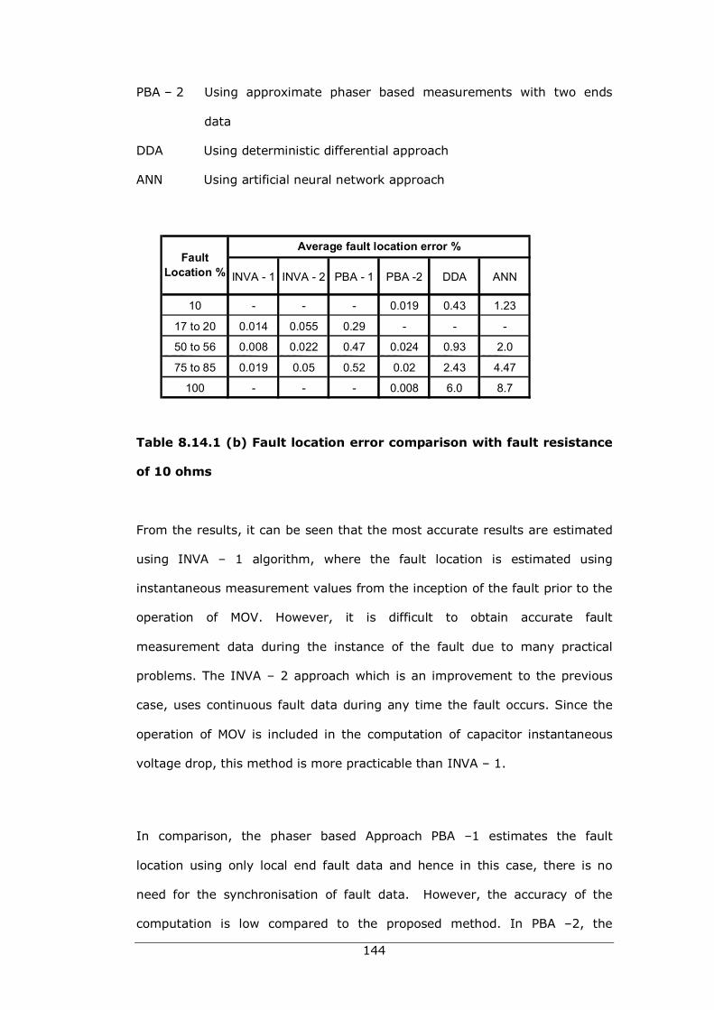
144
PBA – 2 Using approximate phaser based measurements with two ends
data
DDA Using deterministic differential approach
ANN Using artificial neural network approach
Table 8.14.1 (b) Fault location error comparison with fault resistance
of 10 ohms
From the results, it can be seen that the most accurate results are estimated
using INVA – 1 algorithm, where the fault location is estimated using
instantaneous measurement values from the inception of the fault prior to the
operation of MOV. However, it is difficult to obtain accurate fault
measurement data during the instance of the fault due to many practical
problems. The INVA – 2 approach which is an improvement to the previous
case, uses continuous fault data during any time the fault occurs. Since the
operation of MOV is included in the computation of capacitor instantaneous
voltage drop, this method is more practicable than INVA – 1.
In comparison, the phaser based Approach PBA –1 estimates the fault
location using only local end fault data and hence in this case, there is no
need for the synchronisation of fault data. However, the accuracy of the
computation is low compared to the proposed method. In PBA –2, the
INVA - 1 INVA - 2 PBA - 1 PBA -2 DDA ANN
10 - - - 0.019 0.43 1.23 17 to 20 0.014 0.055 0.29 - - - 50 to 56 0.008 0.022 0.47 0.024 0.93 2.0 75 to 85 0.019 0.05 0.52 0.02 2.43 4.47
100 - - - 0.008 6.0 8.7
Fault Location %
Average fault location error %
145
accuracy of the fault location is very similar to the proposed method, but this
algorithm is based on assuming the fault is purely resistive. (No phase
difference between the total fault current and the fault voltage.) Therefore, it
is extremely difficult to apply this method in real fault locations and has
limited space for further improvements.
It can be seen from Table 8.14.1 (a) and (b), that with Deterministic
Differential Approach (DDA) the fault location accuracy is significantly lower
compared to INVA-2, where both methods are based on time domain signal
measurements. In DDA, lower accuracy may be mainly due to the low
sampling rate chosen. (16 samples per cycle) With a lower sampling rate, a
piecewise linear approximation which is used in computing a SCU
instantaneous voltage drop will not be accurate. During the testing of the new
algorithm, several sampling rates (from 1 KHz onwards) have been applied,
and a higher sampling rate has been chosen in order to compute the fault
distance very accurately.
Artificial Neural Network approach (ANN) is simple and is much more robust
compared to the other algorithms stated in this paper, and can be applied to
different network configurations [15]. However, using the ANN technique, the
input and output relationship must be established with a larger number of
fault data during the training process. From Table 8.14.1 (a) and (b), it can
be noted that the accuracy of the fault location (± 10%) is much higher than
other methods stated in this paper.
146
8.15 Summary
The results of several fault location algorithms developed in this research
work on series compensated transmission lines are compared with algorithms
developed by other authors. First this chapter describes the transmission line
model and the environment in which the algorithm was implemented and
tested to compare results. Finally, statistical results of fault location error is
summarised and tabulated for each fault location algorithm described in this
research work.
147
Chapter 9.0
Further improvements
to Fault location algorithm
9.1 Applying new algorithm to long transmission lines
One of the major problem with the new algorithm developed using time
domain approach for series compensated transmission lines is that the shunt
capacitive currents dominant in long lines can affect the accuracy of fault
location [2, 18, 38, 39, 54]. This is because, the preset algorithms do not
include the shunt currents when estimation the fault distance and therefore
the algorithms developed in this research works require further improvements
to incorporate shunt capacitive currents for long high voltage transmission
network cases. Following sections described how to overcome this problem
and suggest modifications to current fault location algorithm.
Modelling of long transmission line with shunt capacitance is described in
Chapter 2 and this mathematical relation between voltage and current at any
given point x is derived using standing wave equations in Chapter 4 and
further fault location equation in time domain is derived in Chapter 6.
Considering the above facts, it is possible to develop an improvement to
present algorithm in application of long transmission lines.
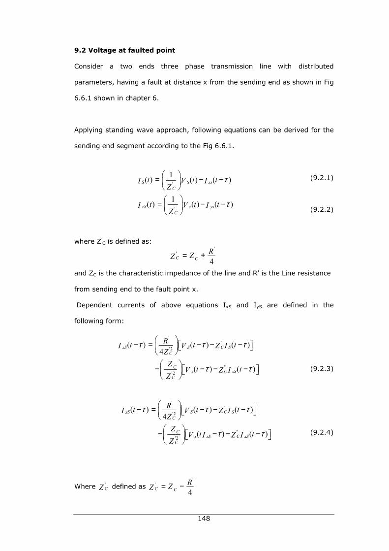
148
9.2 Voltage at faulted point
Consider a two ends three phase transmission line with distributed
parameters, having a fault at distance x from the sending end as shown in Fig
6.6.1 shown in chapter 6.
Applying standing wave approach, following equations can be derived for the
sending end segment according to the Fig 6.6.1.
(9.2.1)
(9.2.2)
where Z’C is defined as:
and ZC is the characteristic impedance of the line and R’ is the Line resistance
from sending end to the fault point x.
Dependent currents of above equations IxS and IyS are defined in the
following form:
(9.2.3)
(9.2.4)
Where "CZ defined as
''
4C CRZZ −=
'
'
1( ) ( ) ( )
1( ) ( ) ( )
S xsSC
xS ysxC
t t tVI IZ
t t tVI IZ
τ
τ
= − − = − −
''
4C CRZZ +=
'"
'2
"'2
( ) ( ) ( )4
( ) ( )
xS C SSC
CC xSx
C
Rt t tVI Z IZZ
t tV Z IZ
τ τ τ
τ τ
− = − − − − − − −
'"
'2
"'2
( ) ( ) ( )4
( ) ( )
xS C SSC
CxS C xSx
C
Rt t tVI Z IZZ
t tV I Z IZ
τ τ τ
τ τ
− = − − − − − − −
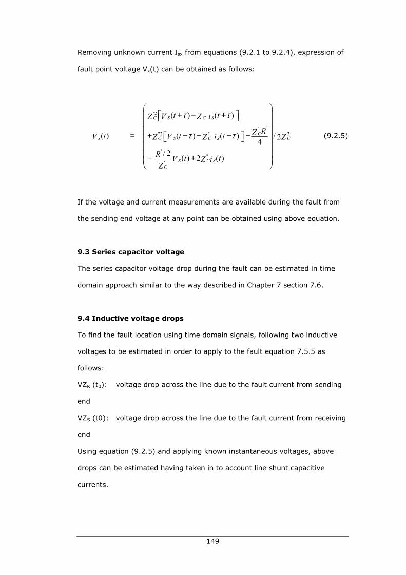
149
Removing unknown current Isx from equations (9.2.1 to 9.2.4), expression of
fault point voltage Vx(t) can be obtained as follows:
(9.2.5)
If the voltage and current measurements are available during the fault from
the sending end voltage at any point can be obtained using above equation.
9.3 Series capacitor voltage
The series capacitor voltage drop during the fault can be estimated in time
domain approach similar to the way described in Chapter 7 section 7.6.
9.4 Inductive voltage drops
To find the fault location using time domain signals, following two inductive
voltages to be estimated in order to apply to the fault equation 7.5.5 as
follows:
VZR (t0): voltage drop across the line due to the fault current from sending
end
VZS (t0): voltage drop across the line due to the fault current from receiving
end
Using equation (9.2.5) and applying known instantaneous voltages, above
drops can be estimated having taken in to account line shunt capacitive
currents.
'2 '
''"2 " 2
'"
'
( ) ( )
( ) ( ) ( ) / 24/ 2 ( ) 2 ( )
C CS S
CC C Cx S S
CS SC
t tV iZ Z
RZt t tV V iZ Z Z
R t tV iZZ
τ τ
τ τ
+ − +
= + − − − − − +
150
9.5 Estimation of fault location
Having known all the instantaneous voltage drops on the right side of
equation 7.5.5, fault location can be estimated for a given time instant t0 .
9.6 Algorithm evaluation
During this research work, this improvement has been tested using limited
cases of fault on two ends transmission network successfully, and the results
can not be quantified without conducting more tests considering many more
variations.
9.7 Parallel transmission lines
During this research works, further investigations have been carried out for
application of currently developed algorithms to more complicated
transmission networks. A new transmission line impedance matrix need to be
derived for developing network equations for parallel line case. If the mutual
effects between parallel lines (Line A and Line B) are considered, new
transmission impedance matrix will have the dimension of 6x 6.
Suppose that line A and B are parallel to each other and having vertical
configuration, line phase to phase mutual effects can be considered as
predominant, and mutual effects of adjacent conductors between lines can be
included to simulate the parallel transmission lines [19].
Using new line impedance matrix, fault equations similar to single line fault
location algorithm can be developed and solve to estimate the location of
fault. Details of the algorithm development for two ends double transmission
lines is presented by this author in 2005 at IEEE Tencon 05 Melbourne,
Australia 19].
151
The initial trails for the test case of parallel transmission network have been
tested with the newly developed algorithm showing encouraging results.
9.8 Summary
Modelling of long transmission lines with shunt capacitance is described in this
chapter as a further improvement to the current time domain fault location
algorithm. Further investigations have been carried out for application of this
fault location algorithm for parallel transmission line networks. The method of
new improvements s was presented in detail by this author in 2005 at IEEE
Tencon 05 conference organised by Melbourne University, Australia.
152
Chapter 10.0
Conclusions
Although great efforts have been undertaken previously by many researchers
aiming to solve the problems of detecting and locating fault in transmission
networks, Many problems still remain as challenges in modern management
of power networks due to the continuous advances in interconnected power
system networks. This research work has contributed in solving many
problems associated with series compensated transmission lines and
developing of new accurate algorithm to estimate fault location.
In order to develop a device which can be used in the power industry, detailed
research was conducted on existing fault location algorithms in line with
application to series compensated lines. It was concluded that phasor based
algorithms developed on the basis of apparent impedance measurements are
not sufficiently accurate for estimating fault location in basic series var
compensated transmission lines.
In chapter 3, a new phasor based fault location algorithm is proposed for
series compensated transmission line using approximate phasor equivalent for
series compensating devices. However, it was proven that the accuracy of
fault location is very much limited and is highly dependant on the type of
transmission network and the type of series compensating device used in the
network.
153
It was identified that operations of series compensation devices produces non
sinusoidal fault signals therefore accurate phasors cannot be obtained to
estimate the location of fault.
To solve this problem, in Chapter 7, a new fault location algorithm is
developed using time domain approach to estimate fault distance on series
compensated transmission lines with high accuracy.
The proposed new approach reveals that accuracy of the fault location in such
lines is highly dependant on the estimation of voltage drop in the series
compensation device during the fault prior to the location of the fault. With
the new method presented in this thesis, it was shown that series capacitor
voltage drop can be estimated in most fault cases with high accuracy which
leads to a in estimating the fault distance more accurately.
The new algorithm was tested with two ends transmission network with series
compensation device located at the middle of the line. The series
compensation device comprises of a series capacitor and Metal Oxide Varistor
(MOV) with spark gap to protect the MOV against over heating. The line
voltage is 400KV and total length is 300 KM.
After simulating the fault on EMTP/ATP software, fault signals were applied to
the new algorithm for estimating the fault distance. Statistical results
obtained for this model shows that the average accuracy of fault location with
new fault location algorithm is more than 99.8%.
Further it was proven that present algorithm can be improved to solve
number of practical issues implementing of this algorithm:
154
• Location of SCU
• Locating fault with respect to SCU
• Multiple SCU devices
• Spark gap operation
• Data sampling rate
• Data synchronising error
The validity of the new algorithm is proven in chapter 8 showing statistical
test results of new algorithm with number of variations in comparison to the
results obtained from algorithms developed by other authors.
At this stage, the present algorithm is developed for short transmission lines
considering the mutual effects of RL network and the line shunt capacitance
are disregarded during the estimation of fault distance. In the practical world,
high voltage long transmission lines have considerable shunt capacitive
currents, and in such cases, the estimation of fault location error using this
algorithm leads to better results than obtained previously.
This problem is identified in the present research work and improvement has
been suggested in the last chapter. Even though, basic testing has been
conducted in this research on this issue showing positive outcomes, the final
results can not be quantified without further testing.
155
Finally, future improvements are suggested to this fault location algorithm on
the following issues that were not considered during this research:
• Developing this algorithm further for Flexible AC Transmission System
(FACTS).
• Application to teed transmission network.
• Searching mathematical solutions to synchronise sending and receiving
ends signals accurately to minimise the fault location error.
156
BIBILOGRAPHY
[1] S. K. Kapuduwage and M. Al-Dabbadh, "A New Simplified Fault Location Algorithm for Series Compensated Transmission lines" in AUPEC 2002 Monash University, Melbourne, 2002.
[2] M. M. Saha, K. Wikstrom, J. Izykowski, and E. Rosolowski, "A new accurate fault locating algorithm for series compensated lines" IEEE Trans. on Power Delivery, vol. 14, pp. 798-797, July 1999.
[3] K. Zimmerman and D. Costello, "Impedance-based fault location experience", pp. 211-226, 2005.
[4] W. J. Cheong and R. K. Aggarwal, "A novel fault location technique based on current signals only for thyristor controlled series compensated transmission lines using wavelet analysis and self organising map neural networks", Vol.1, pp. 224-227, 2004.
[5] Q. Zhang and D. W. P. Thomas, "Accurate fault location algorithms for two parallel transmission line using one-end data", vol.1,pp. 527-530, 2001.
[6] S. K. Kapuduwage and M. Al-Dabbadh, "One End Simplified Fault Location Algorithm Using Instantaneous Values for Series Compensated High Voltage Transmission lines" in AUPEC 2004 University of Queensland, 2004.
[7] H. Heng-xu, Z. Bao-hui, and L. Zhi-lai, "A novel principle of single-ended fault location technique for EHV transmission lines" Power Delivery, IEEE Transactions on, vol. 18, pp. 1147-1151, 2003.
[8] M. Leclere, J. Lambert, R. Lord, and Y. Hebert, "New adaptive algorithm for precise voltage phasor measurement in a series compensated network", IEEE Canadian Conference, vol.1, pp. 397-400, 1998.
[9] J. Lambert, A. G. Phadke, and D. McNabb, "Accurate voltage phasor measurement in a series-compensated network", Power Delivery, IEEE Transactions on, vol. 9, pp. 501-509, 1994.
[10] M. Al-Dabbagh and S. K. Kapuduwage, "A Novel Efficient Fault Location Algorithm for Series Compensated High Voltage Transmission lines", in SCI 2003 - 7th World Multi-Conference on Systematics, Orlando, Florida, USA, 2003, pp. 20-25.
[11] Alternative Transients Program Rule Book, The Leuven EMTP Center (LEC), July 1987.
[12] Hingoraani and N. G, Understanding FACTS: Concept and Technology of Flexible AC Transmission Systems: New York, IEEE Press,C2000, 2000.
[13] S. S. Moorthy, Transmission Line Modelling: Melbourne Co-Op book shop, RMIT University, Melbourne, Australia, 2001 Edition.
[14] S. K. Kapuduwage, M. Al-Dabbadh, "Using Instantaneous Values for Estimating Fault Location on Series Compensated Transmission Lines", Electric Power Systems Research, vol. 76, pp. 25-32, 2005.
[15] D. Novosel, B. Bachmann, D. Hart, Y. Hu, and M. M. Saha, "Algorithms for locating faults on series compensated lines using neural network
157
and deterministic methods", Power Delivery, IEEE Transactions on, vol. 11, pp. 1728-1736, 1996.
[16] M. Al-Dabbagh and S. K. Kapuduwage, "Fault Impedance Variation on Accuracy of Fault location algorithm for Series Compensated High Voltage Transmission Lines", WSEAS Conference, Izmir, Turkey, 2004.
[17] M. Al-Dabbagh and S. K. Kapuduwage, "Effects of Dynamic Fault Impedance Variation on Accuracy of Fault Location for Series Compensated Transmission lines" WSEAS Transactions on Circuit and Systems 8, vol.3, pp. PP 1653-1657, 2004.
[18] S. K. Kapuduwage and M. Al-Dabbadh, "Influence of Inserting FACTS Series Capacitor on High Voltage Transmission lines on Estimation of Fault Location" in AUPEC 2005, Hobart, Tasmania, Australia, pp. 621-625, 2005.
[19] S. K. Kapuduwage and M. Al-Dabbadh, "Development of Efficient Algorithm for Fault Location on Series Compensated Parallel Transmission Lines," in IEEE Tencon 05 Melbourne, Australia, 2005.
[20] P. Ryan, K. Davis, and S. Rawat, "A case study of two-stage fault location,"Reliability Physics Symposium 1992. 30th Annual Proceedings, pp. 332-337, 1992.
[21] E. S. T. E. Din, M. Gilany, M. M. A. Aziz, and D. K. Ibrahim, "An PMU double ended fault location scheme for aged power cables" IEEE Power Engineering Society General Meeting, Vol. 1, pp. 80-86, 2005.
[22] R. Dutra, L. Fabiano, M. M. Saha, and S. Lidstrom, "Fault location on parallel transmission lines with series compensation", IEEE/PES,2004, Transmission and Distribution Conference and Exposition, IEEE/PES, pp. 591-597, 2004.
[23] A. Elhaffar and M. Lehtonen, "Travelling waves based earth fault location in 400 kV transmission network using single end measurement", Power Engineering LESCOPE-04, pp. 53-56, 2004.
[24] C. Y. Evrenosoglu and A. Abur, "Fault location for teed circuits with mutually coupled lines and series capacitors", IEEE, Power Tech Conference Proceedings, Bologna, Vol.3, pp. 1-6, 2003.
[25] C. Y. Evrenosoglu and A. Abur, "Travelling wave based fault location for teed circuits," Power Delivery, IEEE Transactions on, vol. 20, pp. 1115-1121, 2005.
[26] J. Izykowski, E. Rosolowski, and M. Saha, "Adaptive digital distance algorithm for parallel transmission lines" in Power Tech Conference Proceedings, 2003 IEEE Bologna, Vol.2, pp 1-6, 2003.
[27] A. T. Johns, P. J. Moore, and R. Whittard, "New technique for the accurate location of earth faults on transmission systems," Generation, Transmission and Distribution, IEE Proceedings-, vol. 142, pp. 119-127, 1995.
[28] L. Kai-Ping, L. Chih-Wen, Y. Chi-Shan, and J. A. Jiang, "Transmission network fault location observability with minimal PMU placement", Power Delivery, IEEE Transactions on, vol. 21, pp. 1128-1136, 2006.
[29] M. Kezunovic and B. Perunicic, "Automated transmission line fault analysis using synchronized sampling at two ends", Power Systems, IEEE Transactions on, vol. 11, pp. 441-447, 1996.
[30] C.-S. Yu, C.-W. Liu, J.-Z. Yang, and J.-A. Jiang, "New Fourier filter algorithm for series compensated transmission lines" in Power System Technology, 2002. Proceedings. PowerCon 2002. International Conference, vol.4, pp. 2556-2560, 2002.
[31] S. K. Kapuduwage and M. Al-Dabbadh, "A Novel Technic for Estimating Fault Location on Series Compensated Transmission Lines Based on Tine-Domain Analysis", International Journal of Emerging Electric Power Systems, 26/09/2006 2006.
158
[32] K.-T. Cheng, "Transition fault testing for sequential circuits", Computer-Aided Design of Integrated Circuits and Systems, IEEE Transactions on, vol. 12, pp. 1971-1983, 1993.
[33] A.T. Johns, L.L.Lai, M. El-Hami, and D. J. Daruvala, "New approch to directional fault location for overhead power distribution feeders", IEE Procedings-C, vol. 138, pp. 351-357, July 1999.
[34] C.-S. Yu, C.-W. Liu, S.-L. Yu, and J.-A. Jiang, "A new PMU-based fault location algorithm for series compensated lines", Power Delivery, IEEE Transactions on, vol. 17, pp. 33-46, 2002.
[35] F. Ghassemi, J. Goodarzi, and A. T. Johns, "Method to improve digital distance relay impedance measurement when used in series compensated lines protected by a metal oxide varistor", Generation, Transmission and Distribution, IEE Proceedings, vol. 145, pp. 403-408, 1998.
[36] S. K. Kapuduwage, M. Al-Dabbadh, "Using Instantaneious Values for Estimating Fault Location on Series Compensated Transmissin Lines", Electric Power Systems Research, vol. 76, pp. 25-32, 2005.
[37] S. K. Kapuduwage and M. Al-Dabbadh, "A New Method for Estimating Fault Location on Series Compensated High Voltage Transmission lines", Engineering Confrence RMIT University, Melbourne, 2003.
[38] M. M. Saha, K. Wikstrom, J. Izykowski, and E. Rosolowski, "New concept for fault location in series-compensated parallel lines", vol.2, pp. 769-774, 2001.
[39] S. K. Kapuduwage and M. Al-Dabbadh, "A Novel Thechines for Estimating Fault Location on Series Compensated Transmission Lines Based on Tine-Domain Analysis", International Journal of Emerging Electric Power Systems, Sep. 2006.
[40] J. Urbanek, R. J. Piwko, E. V. Larsen, B. L. Damsky, B. C. Furumasu, W. Mittlestadt, and J. D. Eden, "Thyristor controlled series compensation prototype installation at the Slatt 500 kV substation", Power Delivery, IEEE Transactions on, vol. 8, pp. 1460-1469, 1993.
[41] C.-S. Yu, C.-W. Liu, and J.-A. Jiang, "A new fault location algorithm for series compensated lines using synchronized phasor measurements" in Power Engineering Society Summer Meeting, 2000. IEEE, vol. 3, pp. 1350-1354, 2000.
[42] Accurate Transmission Line Fault Location: HP Hewlett Packard Application Note 1276.
[43] A. T. Johns, Song, and Yong-Hua, flexible AC Transmision Systems (FACTS): London,Institution of Electrical Engineers, 1999.
[44] M.S. Sachdev and R. Aggarwal, "A technique for estimating line fault from digital distance relay measurements", IEEE Trans. on Power Delivery, Vol. 17, PP 121-129, January 1988.
[45] I.J. Nagrath and D. P. Kothari, ModernPower System Analysis: Tata Mc-Graw Hill,New Dehli, 1980.
[46] D. L. Goldsworthy, "A Linearized model for MOV-protected series capacitors," IEEE Trans. Power System, vol 2, pp 953-958, Nov. 1987.
[47] Alternative Transients Program Rule Book,The Leuven EMTP Center (LEC), Sep. 1991.
[48] L. Daqing, "Computer-controlled test station for HP data acquisition system products", pp. 465-468,1994.
[49] Power System Blockset User's Guide,: Natick, MA: The MathWorks, 1998.
[50] MATLAB 6.5 Release 12.1, Help Reference 2003, The MathWorks, Inc. [51] W. J. Cheong and R. K. Aggarwal, "Accurate fault location in high
voltage transmission systems comprising an improved thyristor controlled series capacitor model using wavelet transforms and neural network", vol.2, pp. 840-845, 2002.
159
[52] S. S. Mohamed, E. F. El-Saadany, T. K. Abdel-Galil, and M. M. A. Salama, "ANN-based technique for fault location estimation using TLS-ESPRIT", Vol. 3, pp. 1090-1094, 2003.
[53] H. Dommel, Electromagnetic Transient Program: Protland,OR,BPA, 1986.
[54] C. Zheng, L. Chengmu, S. Jinxi, and W. Xinrong, "A fault location algorithm for transmission line based on distributed parameter", Developments in Power System Protection, IEE, pp. 411-413, 2001.
[55] S. Hongchun, S. Dajun, and C. Xueyun, "A new electromagnetic transient simulation method for faults in complex power system," in Power System Technology, 2002. Proceedings. PowerCon 2002. International Conference, vol.4, pp. 2645-2651, 2002.
[56] M. Al-Dabbagh and S. K. Kapuduwage, "A New Method for Estimation of Fault Location on Series Compensated High Voltage Transmission lines" in EuroPES 2004 Power & Energy Rhodes, Greece, 2004.
[57] M. Al-Dabbagh and S. K. Kapuduwage, "Effects of Dynamic Fault Impedance Variation on Accuracy of Fault Location for Series Compensated Transmission lines", WSEAS Transactions on Circuit and Systems 8,Vol 3, pp. 1653-1657, Oct. 2004.
[58] S. Li, C. Fan, W. Yu, H. Cai, and K. K. Li, "A new phase measurement unit (PMU) based fault location algorithm for double circuit lines", Vol.1, pp. 188-191, 2004.
[59] O. Nigol, "Methods for analyzing the performance of gapless metal oxide surge arresters", Power Delivery, IEEE Transactions on, vol. 7, pp. 1256-1264, 1992.
[60] T. Adu, "An accurate fault classification technique for power system monitoring devices," Power Delivery, IEEE Transactions on, vol. 17, pp. 684-690, 2002.
[61] C. Ching-Shan, L. Chih-Wen, and J. Joe-Air, "Three-terminal transmission line protection using synchronized voltage and current phasor measurements", Transmission and Distribution Conference, vol.3, pp. 1727-1732, 2002.
[62] H. Zijun, C. Yunping, and G. Qingwu, "A protection and fault location scheme for EHV line with series capacitor based on travelling waves and wavelet analysis", Power System Technology Proceedings, vol.1, pp. 290-294, 2002.
[63] Z. Chen and J. C. Maun, "Artificial neural network approach to single-ended fault locator for transmission lines", Power Systems, IEEE Transactions on, vol. 15, pp. 370-375, 2000.
[64] User Manual for ATPDraw for Windows version 3.5 - User Manual. [65] ATP Analyzer 3.11 - Reference Manual 2005.
160
Appendix A
A: Basic data structure of the common EMTP Simulation
Special request cardMiscellaneous data parameters
BEGIN NEW DATA CASE
Transfer functions ( S or Z blocks.)SourcesSupplement variables and devicesOutputsInitial conditions
Branch cards
Switches
BLANK line ending branch inputs
TACS HYBRID
BLANK line ending TACS inputs
BLANK line ending switch inputsSources
BLANK line ending source inputs
Plotting - user requestsFOURIER analysis
BLANK line ending plotting inputs
BEGIN NEW DATA CASEBLANK card to end the data case
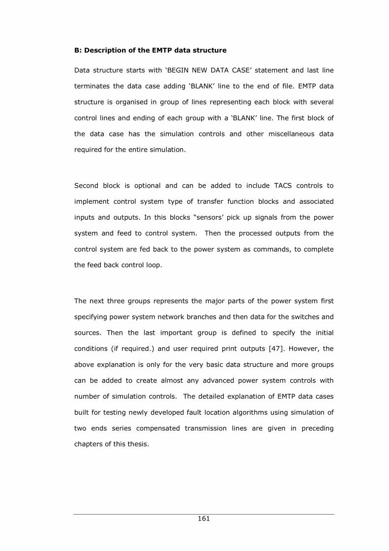
161
B: Description of the EMTP data structure
Data structure starts with ‘BEGIN NEW DATA CASE’ statement and last line
terminates the data case adding ‘BLANK’ line to the end of file. EMTP data
structure is organised in group of lines representing each block with several
control lines and ending of each group with a ‘BLANK’ line. The first block of
the data case has the simulation controls and other miscellaneous data
required for the entire simulation.
Second block is optional and can be added to include TACS controls to
implement control system type of transfer function blocks and associated
inputs and outputs. In this blocks “sensors’ pick up signals from the power
system and feed to control system. Then the processed outputs from the
control system are fed back to the power system as commands, to complete
the feed back control loop.
The next three groups represents the major parts of the power system first
specifying power system network branches and then data for the switches and
sources. Then the last important group is defined to specify the initial
conditions (if required.) and user required print outputs [47]. However, the
above explanation is only for the very basic data structure and more groups
can be added to create almost any advanced power system controls with
number of simulation controls. The detailed explanation of EMTP data cases
built for testing newly developed fault location algorithms using simulation of
two ends series compensated transmission lines are given in preceding
chapters of this thesis.
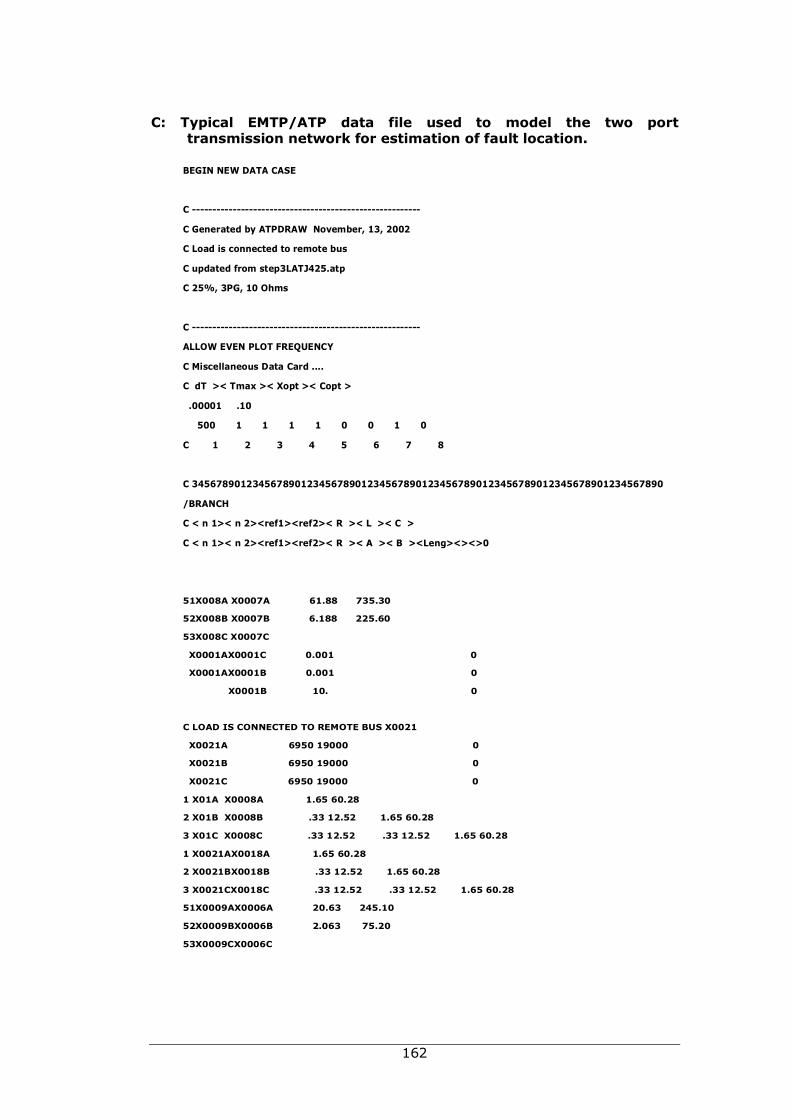
162
C: Typical EMTP/ATP data file used to model the two port transmission network for estimation of fault location.
BEGIN NEW DATA CASE
C --------------------------------------------------------
C Generated by ATPDRAW November, 13, 2002
C Load is connected to remote bus
C updated from step3LATJ425.atp
C 25%, 3PG, 10 Ohms
C --------------------------------------------------------
ALLOW EVEN PLOT FREQUENCY
C Miscellaneous Data Card ....
C dT >< Tmax >< Xopt >< Copt >
.00001 .10
500 1 1 1 1 0 0 1 0
C 1 2 3 4 5 6 7 8
C 345678901234567890123456789012345678901234567890123456789012345678901234567890
/BRANCH
C < n 1>< n 2><ref1><ref2>< R >< L >< C >
C < n 1>< n 2><ref1><ref2>< R >< A >< B ><Leng><><>0
51X008A X0007A 61.88 735.30
52X008B X0007B 6.188 225.60
53X008C X0007C
X0001AX0001C 0.001 0
X0001AX0001B 0.001 0
X0001B 10. 0
C LOAD IS CONNECTED TO REMOTE BUS X0021
X0021A 6950 19000 0
X0021B 6950 19000 0
X0021C 6950 19000 0
1 X01A X0008A 1.65 60.28
2 X01B X0008B .33 12.52 1.65 60.28
3 X01C X0008C .33 12.52 .33 12.52 1.65 60.28
1 X0021AX0018A 1.65 60.28
2 X0021BX0018B .33 12.52 1.65 60.28
3 X0021CX0018C .33 12.52 .33 12.52 1.65 60.28
51X0009AX0006A 20.63 245.10
52X0009BX0006B 2.063 75.20
53X0009CX0006C
163
X0001AX0001C 0.001 0
X0001AX0001B 0.001 0
X0001B 10. 0
C LOAD IS CONNECTED TO REMOTE BUS X0021
X0021A 6950 19000 0
X0021B 6950 19000 0
X0021C 6950 19000 0
1 X01A X0008A 1.65 60.28
2 X01B X0008B .33 12.52 1.65 60.28
3 X01C X0008C .33 12.52 .33 12.52 1.65 60.28
1 X0021AX0018A 1.65 60.28
2 X0021BX0018B .33 12.52 1.65 60.28
3 X0021CX0018C .33 12.52 .33 12.52 1.65 60.28
51X0009AX0006A 20.63 245.10
52X0009BX0006B 2.063 75.20
53X0009CX0006C
X08AX008A 38. 0
X0006BX008B 38. 0
X0006CX008C 38. 0
C MOV DATA INSERTED
92 X09AX008A 5555. 1st card of 1st of 3 ZnO arrest
C VREF VFLASH VZERO COL
330000. -1.0 0.0 2.0
C COEF EXPON VMIN
2200. 23. 0.5
9999.
92X0006BX008B X09AX008A 5555. Phase "b" ZnO is copy of "a"
92X0006CX008C X09AX008A 5555. Phase "c" ZnO is copy of "b"
/SWITCH
C < n 1>< n 2>< Tclose ><Top/Tde >< Ie ><Vf/CLOP >< type >
X0008AX0009A MEASURING 1
X0008BX0009B MEASURING 1
X0008CX0009C MEASURING 1
X0006AX0001A .035 .5 0
X0006BX0001B .035 .5 0
X0006CX0001C .035 .5 0
X0021AX0007A MEASURING 1
X0021BX0007B MEASURING 1
164
X0021CX0007C MEASURING 1
X08AX0006A MEASURING 0
X09AX0006A MEASURING 0
/SOURCE
C < n 1><>< Ampl. >< Freq. ><Phase/T0>< A1 >< T1 >< TSTART >< TSTOP >
14X01A 0 327000. 50. -1. 10.
14X01B 0 327000. 50. -120. -1. 10.
14X01C 0 327000. 50. 120. -1. 10.
14X0018A 0 327000. 50. -1. 10.
14X0018B 0 327000. 50. -120. 1. 10.
14X0018C 0 327000. 50. 120. 1. 10.
BLANK BRANCH
BLANK SWITCH
BLANK SOURCE
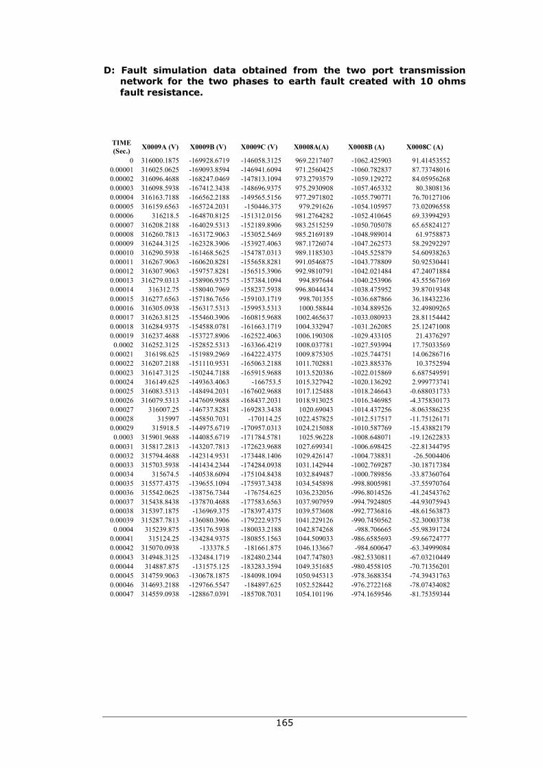
165
D: Fault simulation data obtained from the two port transmission network for the two phases to earth fault created with 10 ohms fault resistance.
TIME (Sec.) X0009A (V) X0009B (V) X0009C (V) X0008A(A) X0008B (A) X0008C (A)
0 316000.1875 -169928.6719 -146058.3125 969.2217407 -1062.425903 91.41453552 0.00001 316025.0625 -169093.8594 -146941.6094 971.2560425 -1060.782837 87.73748016 0.00002 316096.4688 -168247.0469 -147813.1094 973.2793579 -1059.129272 84.05956268 0.00003 316098.5938 -167412.3438 -148696.9375 975.2930908 -1057.465332 80.3808136 0.00004 316163.7188 -166562.2188 -149565.5156 977.2971802 -1055.790771 76.70127106 0.00005 316159.6563 -165724.2031 -150446.375 979.291626 -1054.105957 73.02096558 0.00006 316218.5 -164870.8125 -151312.0156 981.2764282 -1052.410645 69.33994293 0.00007 316208.2188 -164029.5313 -152189.8906 983.2515259 -1050.705078 65.65824127 0.00008 316260.7813 -163172.9063 -153052.5469 985.2169189 -1048.989014 61.9758873 0.00009 316244.3125 -162328.3906 -153927.4063 987.1726074 -1047.262573 58.29292297 0.00010 316290.5938 -161468.5625 -154787.0313 989.1185303 -1045.525879 54.60938263 0.00011 316267.9063 -160620.8281 -155658.8281 991.0546875 -1043.778809 50.92530441 0.00012 316307.9063 -159757.8281 -156515.3906 992.9810791 -1042.021484 47.24071884 0.00013 316279.0313 -158906.9375 -157384.1094 994.897644 -1040.253906 43.55567169 0.00014 316312.75 -158040.7969 -158237.5938 996.8044434 -1038.475952 39.87019348 0.00015 316277.6563 -157186.7656 -159103.1719 998.701355 -1036.687866 36.18432236 0.00016 316305.0938 -156317.5313 -159953.5313 1000.58844 -1034.889526 32.49809265 0.00017 316263.8125 -155460.3906 -160815.9688 1002.465637 -1033.080933 28.81154442 0.00018 316284.9375 -154588.0781 -161663.1719 1004.332947 -1031.262085 25.12471008 0.00019 316237.4688 -153727.8906 -162522.4063 1006.190308 -1029.433105 21.4376297 0.0002 316252.3125 -152852.5313 -163366.4219 1008.037781 -1027.593994 17.75033569
0.00021 316198.625 -151989.2969 -164222.4375 1009.875305 -1025.744751 14.06286716 0.00022 316207.2188 -151110.9531 -165063.2188 1011.702881 -1023.885376 10.3752594 0.00023 316147.3125 -150244.7188 -165915.9688 1013.520386 -1022.015869 6.687549591 0.00024 316149.625 -149363.4063 -166753.5 1015.327942 -1020.136292 2.999773741 0.00025 316083.5313 -148494.2031 -167602.9688 1017.125488 -1018.246643 -0.688031733 0.00026 316079.5313 -147609.9688 -168437.2031 1018.913025 -1016.346985 -4.375830173 0.00027 316007.25 -146737.8281 -169283.3438 1020.69043 -1014.437256 -8.063586235 0.00028 315997 -145850.7031 -170114.25 1022.457825 -1012.517517 -11.75126171 0.00029 315918.5 -144975.6719 -170957.0313 1024.215088 -1010.587769 -15.43882179 0.0003 315901.9688 -144085.6719 -171784.5781 1025.96228 -1008.648071 -19.12622833
0.00031 315817.2813 -143207.7813 -172623.9688 1027.699341 -1006.698425 -22.81344795 0.00032 315794.4688 -142314.9531 -173448.1406 1029.426147 -1004.738831 -26.5004406 0.00033 315703.5938 -141434.2344 -174284.0938 1031.142944 -1002.769287 -30.18717384 0.00034 315674.5 -140538.6094 -175104.8438 1032.849487 -1000.789856 -33.87360764 0.00035 315577.4375 -139655.1094 -175937.3438 1034.545898 -998.8005981 -37.55970764 0.00036 315542.0625 -138756.7344 -176754.625 1036.232056 -996.8014526 -41.24543762 0.00037 315438.8438 -137870.4688 -177583.6563 1037.907959 -994.7924805 -44.93075943 0.00038 315397.1875 -136969.375 -178397.4375 1039.573608 -992.7736816 -48.61563873 0.00039 315287.7813 -136080.3906 -179222.9375 1041.229126 -990.7450562 -52.30003738 0.0004 315239.875 -135176.5938 -180033.2188 1042.874268 -988.706665 -55.98391724
0.00041 315124.25 -134284.9375 -180855.1563 1044.509033 -986.6585693 -59.66724777 0.00042 315070.0938 -133378.5 -181661.875 1046.133667 -984.600647 -63.34999084 0.00043 314948.3125 -132484.1719 -182480.2344 1047.747803 -982.5330811 -67.03210449 0.00044 314887.875 -131575.125 -183283.3594 1049.351685 -980.4558105 -70.71356201 0.00045 314759.9063 -130678.1875 -184098.1094 1050.945313 -978.3688354 -74.39431763 0.00046 314693.2188 -129766.5547 -184897.625 1052.528442 -976.2722168 -78.07434082 0.00047 314559.0938 -128867.0391 -185708.7031 1054.101196 -974.1659546 -81.75359344
166
0.03647 110989.4453 -255837.9375 144852.5313 -72.93703461 -2629.772705 2702.985596 0.036479998 111705.3047 -255938.5156 144237.2813 -65.62844849 -2643.814697 2709.718262 0.036490001 112420.25 -256036.5938 143620.4375 -58.27939987 -2657.844482 2716.398438 0.036499999 113134.2734 -256132.1563 143001.9844 -50.89001465 -2671.862061 2723.026123 0.036509998 113847.375 -256225.1875 142381.9375 -43.46041489 -2685.867432 2729.601318 0.036520001 114559.5469 -256315.7031 141760.2969 -35.99072647 -2699.860352 2736.124023 0.036529999 115270.7813 -256403.6875 141137.0781 -28.48106956 -2713.840576 2742.593994 0.036540002 115981.0625 -256489.1563 140512.2813 -20.93157578 -2727.807861 2749.011475
0.03655 116690.3984 -256572.1094 139885.9219 -13.34236717 -2741.762451 2755.376221 0.036559999 117398.7656 -256652.5313 139257.9844 -5.713569164 -2755.704102 2761.688232 0.036570001 118106.1641 -256730.4219 138628.5 1.954691529 -2769.632324 2767.947754
0.03658 118812.5859 -256805.7969 137997.4688 9.662289619 -2783.547363 2774.154541 0.036589999 119518.0313 -256878.625 137364.875 17.40909767 -2797.44873 2780.308594 0.036600001 120222.4766 -256948.9375 136730.7656 25.19499016 -2811.33667 2786.410156
0.03661 120925.9297 -257016.7031 136095.1094 33.01984024 -2825.210938 2792.45874 0.036619999 121628.3672 -257081.9531 135457.9219 40.88351822 -2839.071045 2798.454834 0.036630001 122329.8047 -257144.6563 134819.2188 48.7858963 -2852.917236 2804.397949
0.03664 123030.2109 -257204.8438 134179 56.72685242 -2866.749268 2810.288574 0.036649998 123729.5938 -257262.4844 133537.2813 64.70625305 -2880.566895 2816.126221 0.036660001 124427.9453 -257317.5781 132894.0625 72.72396851 -2894.370117 2821.911133 0.036669999 125125.25 -257370.1563 132249.3438 80.77987671 -2908.158691 2827.643066 0.036680002 125821.5078 -257420.1875 131603.125 88.87384033 -2921.932617 2833.32251
0.03669 126516.7031 -257467.6719 130955.4453 97.0057373 -2935.69165 2838.948975 0.036699999 127210.8359 -257512.625 130306.2813 105.1754303 -2949.435547 2844.522705 0.036710002 127903.8984 -257555.0313 129655.6406 113.3827972 -2963.164307 2850.043457
0.03672 128595.8828 -257594.9063 129003.5469 121.6277084 -2976.877686 2855.511475 0.036729999 129286.7813 -257632.2344 128349.9922 129.9100342 -2990.575684 2860.926514 0.036740001 129976.5859 -257667.0156 127694.9922 138.2296295 -3004.258301 2866.288818
0.03675 130665.2891 -257699.25 127038.5469 146.58638 -3017.925049 2871.598145 0.036759999 131352.8906 -257728.9531 126380.6641 154.9801483 -3031.575928 2876.854492 0.036770001 132039.375 -257756.0938 125721.3594 163.4107971 -3045.210693 2882.058105
0.03678 132724.7344 -257780.7031 125060.6172 171.8782043 -3058.829346 2887.20874 0.036789998 133408.9688 -257802.7656 124398.4688 180.3822327 -3072.431885 2892.306641 0.036800001 134092.0625 -257822.2813 123734.9063 188.9227448 -3086.017822 2897.351563 0.036809999 134774 -257839.2344 123069.9375 197.4996338 -3099.587402 2902.343506 0.036819998 135454.8125 -257853.6563 122403.5781 206.1127319 -3113.140137 2907.282471 0.036830001 136134.4531 -257865.5313 121735.8203 214.7619324 -3126.676025 2912.168701 0.036839999 136812.9219 -257874.8438 121066.6875 223.4470825 -3140.195068 2917.001953 0.036850002 137490.2344 -257881.625 120396.1719 232.1680603 -3153.697021 2921.782227
0.03686 138166.3594 -257885.8438 119724.2813 240.9247284 -3167.181641 2926.509521 0.036869999 138841.2969 -257887.5156 119051.0313 249.7169647 -3180.648926 2931.184082 0.036880001 139515.0469 -257886.625 118376.4297 258.5446167 -3194.098877 2935.805664
0.03689 140187.5938 -257883.2031 117700.4688 267.4075623 -3207.531006 2940.374023 0.036899999 140858.9219 -257877.2188 117023.1719 276.3056641 -3220.945313 2944.889893 0.036910001 141529.0469 -257868.6875 116344.5313 285.2387695 -3234.341797 2949.352539
0.03692 142197.9531 -257857.6094 115664.5625 294.2067566 -3247.720215 2953.762207 0.036929999 142865.625 -257843.9688 114983.2734 303.2095032 -3261.080322 2958.119141 0.036940001 143532.0625 -257827.7813 114300.6641 312.2468872 -3274.422363 2962.423096
0.03695 144197.2656 -257809.0313 113616.7422 321.3187256 -3287.74585 2966.674072 0.036959998 144861.2031 -257787.75 112931.5234 330.4248962 -3301.050781 2970.87207
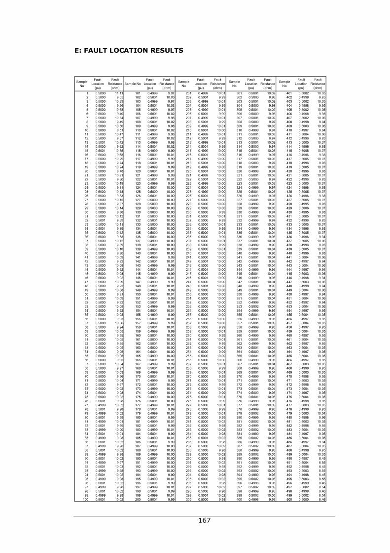
167
E: FAULT LOCATION RESULTS
Sample No
Fault Location
(pu)
Fault Reistance
(ohm)Sample No
Fault Location
(pu)
Fault Reistance
(ohm)
Sample No
Fault Location
(pu)
Fault Reistance
(ohm)
Sample No
Fault Location
(pu)
Fault Reistance
(ohm)
Sample No
Fault Location
(pu)
Fault Reistance
(ohm)1 0.5000 11.11 101 0.4999 9.97 201 0.4999 10.01 301 0.5001 10.02 401 0.5002 10.052 0.5000 9.05 102 0.5001 10.03 202 0.5001 9.99 302 0.5000 9.98 402 0.4998 9.953 0.5000 10.83 103 0.4999 9.97 203 0.4999 10.01 303 0.5001 10.02 403 0.5002 10.054 0.5000 9.26 104 0.5001 10.03 204 0.5001 9.99 304 0.5000 9.98 404 0.4998 9.955 0.5000 10.68 105 0.4999 9.97 205 0.4999 10.01 305 0.5001 10.02 405 0.5002 10.056 0.5000 9.40 106 0.5001 10.02 206 0.5001 9.99 306 0.5000 9.98 406 0.4998 9.957 0.5000 10.54 107 0.4999 9.98 207 0.4999 10.01 307 0.5001 10.02 407 0.5002 10.068 0.5000 9.49 108 0.5001 10.02 208 0.5001 9.99 308 0.5000 9.97 408 0.4998 9.949 0.5000 10.50 109 0.4999 9.98 209 0.4999 10.01 309 0.5001 10.03 409 0.5003 10.06
10 0.5000 9.51 110 0.5001 10.02 210 0.5001 10.00 310 0.4999 9.97 410 0.4997 9.9411 0.5000 10.47 111 0.4999 9.98 211 0.4999 10.01 311 0.5001 10.03 411 0.5004 10.0612 0.5000 9.57 112 0.5001 10.02 212 0.5001 9.99 312 0.5000 9.97 412 0.4996 9.9313 0.5001 10.42 113 0.4999 9.98 213 0.4999 10.01 313 0.5001 10.02 413 0.5005 10.0714 0.5000 9.62 114 0.5001 10.02 214 0.5001 9.99 314 0.5000 9.97 414 0.4996 9.9315 0.5001 10.35 115 0.4999 9.99 215 0.4999 10.00 315 0.5001 10.03 415 0.5005 10.0716 0.5000 9.68 116 0.5001 10.01 216 0.5001 10.00 316 0.4999 9.97 416 0.4996 9.9317 0.5000 10.29 117 0.4999 9.99 217 0.4999 10.00 317 0.5001 10.03 417 0.5005 10.0718 0.5000 9.74 118 0.5001 10.01 218 0.5001 10.00 318 0.5000 9.97 418 0.4996 9.9319 0.5000 10.24 119 0.4999 9.99 219 0.4999 10.00 319 0.5001 10.03 419 0.5005 10.0720 0.5000 9.78 120 0.5001 10.01 220 0.5001 10.00 320 0.4999 9.97 420 0.4996 9.9321 0.5000 10.21 121 0.4999 9.99 221 0.4999 10.00 321 0.5001 10.03 421 0.5005 10.0722 0.5000 9.80 122 0.5001 10.01 222 0.5001 10.00 322 0.5000 9.97 422 0.4996 9.9323 0.5000 10.19 123 0.4999 9.99 223 0.4999 10.00 323 0.5001 10.03 423 0.5005 10.0724 0.5000 9.81 124 0.5001 10.00 224 0.5001 10.00 324 0.4999 9.97 424 0.4996 9.9325 0.5000 10.18 125 0.5000 10.00 225 0.4999 10.00 325 0.5001 10.03 425 0.5005 10.0726 0.5000 9.83 126 0.5001 10.00 226 0.5001 10.00 326 0.4999 9.97 426 0.4996 9.9327 0.5000 10.15 127 0.5000 10.00 227 0.5000 10.00 327 0.5001 10.03 427 0.5005 10.0728 0.5000 9.87 128 0.5000 10.00 228 0.5000 10.00 328 0.4999 9.96 428 0.4995 9.9329 0.5000 10.14 129 0.5000 10.00 229 0.5000 10.00 329 0.5001 10.03 429 0.5006 10.0730 0.5000 9.86 130 0.5000 10.00 230 0.5000 9.99 330 0.4999 9.97 430 0.4995 9.9331 0.5000 10.12 131 0.5000 10.00 231 0.5000 10.01 331 0.5001 10.03 431 0.5005 10.0732 0.5001 9.89 132 0.5001 10.00 232 0.5000 9.99 332 0.4999 9.97 432 0.4996 9.9333 0.5000 10.11 133 0.5000 10.00 233 0.5000 10.01 333 0.5001 10.03 433 0.5005 10.0734 0.5001 9.89 134 0.5001 10.00 234 0.5000 9.99 334 0.4999 9.96 434 0.4996 9.9335 0.5000 10.12 135 0.5000 10.00 235 0.5000 10.01 335 0.5001 10.04 435 0.5005 10.0736 0.5000 9.88 136 0.5001 10.00 236 0.5000 9.99 336 0.4999 9.96 436 0.4996 9.9437 0.5000 10.12 137 0.4999 10.00 237 0.5000 10.01 337 0.5001 10.04 437 0.5005 10.0638 0.5000 9.89 138 0.5001 10.00 238 0.5000 9.99 338 0.4999 9.96 438 0.4996 9.9339 0.5000 10.10 139 0.4999 10.00 239 0.5000 10.01 339 0.5001 10.04 439 0.5005 10.0740 0.5000 9.90 140 0.5001 10.00 240 0.5001 10.00 340 0.4999 9.96 440 0.4996 9.9341 0.5000 10.09 141 0.4999 9.99 241 0.5000 10.00 341 0.5001 10.04 441 0.5004 10.0642 0.5000 9.92 142 0.5001 10.01 242 0.5001 10.00 342 0.4999 9.95 442 0.4997 9.9443 0.5000 10.08 143 0.4999 9.99 243 0.5000 10.00 343 0.5001 10.04 443 0.5004 10.0644 0.5000 9.92 144 0.5001 10.01 244 0.5001 10.00 344 0.4999 9.96 444 0.4997 9.9445 0.5000 10.08 145 0.4999 9.99 245 0.5000 10.00 345 0.5001 10.04 445 0.5003 10.0646 0.5000 9.92 146 0.5001 10.01 246 0.5001 10.00 346 0.4999 9.96 446 0.4998 9.9447 0.5000 10.09 147 0.4999 9.99 247 0.5000 10.00 347 0.5001 10.04 447 0.5003 10.0648 0.5000 9.92 148 0.5001 10.01 248 0.5001 10.00 348 0.4999 9.96 448 0.4998 9.9449 0.5000 10.08 149 0.4999 9.99 249 0.5000 10.00 349 0.5001 10.04 449 0.5004 10.0650 0.5000 9.91 150 0.5001 10.01 250 0.5000 10.00 350 0.4999 9.96 450 0.4997 9.9451 0.5000 10.09 151 0.4999 9.99 251 0.5000 10.00 351 0.5001 10.04 451 0.5004 10.0652 0.5000 9.92 152 0.5001 10.01 252 0.5000 10.00 352 0.4999 9.96 452 0.4997 9.9453 0.5000 10.08 153 0.4999 9.99 253 0.5000 10.00 353 0.5002 10.04 453 0.5004 10.0654 0.5000 9.92 154 0.5001 10.01 254 0.5000 10.00 354 0.4999 9.95 454 0.4997 9.9555 0.5000 10.08 155 0.4999 9.99 255 0.5000 10.00 355 0.5001 10.05 455 0.5004 10.0556 0.5000 9.93 156 0.5001 10.01 256 0.5000 10.00 356 0.4999 9.95 456 0.4997 9.9557 0.5000 10.06 157 0.4999 9.99 257 0.5000 10.00 357 0.5001 10.05 457 0.5004 10.0558 0.5000 9.94 158 0.5001 10.01 258 0.5000 9.99 358 0.4999 9.95 458 0.4997 9.9559 0.5000 10.05 159 0.4999 9.99 259 0.5000 10.01 359 0.5001 10.05 459 0.5004 10.0560 0.5000 9.95 160 0.5001 10.00 260 0.5000 9.99 360 0.4999 9.95 460 0.4997 9.9561 0.5000 10.05 161 0.5000 10.00 261 0.5000 10.01 361 0.5001 10.05 461 0.5004 10.0562 0.5000 9.95 162 0.5001 10.00 262 0.5000 9.99 362 0.4999 9.95 462 0.4997 9.9563 0.5000 10.05 163 0.5000 10.00 263 0.5000 10.01 363 0.5001 10.04 463 0.5004 10.0564 0.5000 9.95 164 0.5001 10.00 264 0.5000 9.99 364 0.5000 9.96 464 0.4997 9.9565 0.5000 10.05 165 0.4999 10.00 265 0.5000 10.00 365 0.5001 10.05 465 0.5004 10.0566 0.5000 9.95 166 0.5001 10.01 266 0.5000 10.00 366 0.4999 9.95 466 0.4997 9.9567 0.5000 10.04 167 0.4999 9.99 267 0.5000 10.01 367 0.5001 10.04 467 0.5003 10.0568 0.5000 9.97 168 0.5001 10.01 268 0.5000 9.99 368 0.4999 9.96 468 0.4998 9.9569 0.5000 10.03 169 0.4999 9.99 269 0.5000 10.01 369 0.5001 10.04 469 0.5003 10.0570 0.5000 9.96 170 0.5001 10.01 270 0.5000 9.99 370 0.4999 9.96 470 0.4998 9.9571 0.5000 10.04 171 0.4999 9.99 271 0.5000 10.01 371 0.5001 10.04 471 0.5003 10.0572 0.5000 9.97 172 0.5001 10.00 272 0.5000 9.99 372 0.4999 9.96 472 0.4998 9.9573 0.5000 10.02 173 0.4999 10.00 273 0.5000 10.01 373 0.5001 10.04 473 0.5004 10.0574 0.5000 9.98 174 0.5001 10.00 274 0.5000 9.99 374 0.5000 9.96 474 0.4997 9.9575 0.5000 10.02 175 0.4999 10.00 275 0.5000 10.01 375 0.5001 10.05 475 0.5004 10.0576 0.5001 9.98 176 0.5001 10.00 276 0.5000 9.99 376 0.4999 9.95 476 0.4998 9.9577 0.4999 10.02 177 0.4999 10.01 277 0.5000 10.01 377 0.5001 10.05 477 0.5003 10.0578 0.5001 9.98 178 0.5001 9.99 278 0.5000 9.99 378 0.4999 9.95 478 0.4998 9.9579 0.4999 10.02 179 0.4999 10.01 279 0.5000 10.01 379 0.5002 10.05 479 0.5003 10.0480 0.5001 9.99 180 0.5001 9.99 280 0.5000 9.99 380 0.4999 9.95 480 0.4998 9.9681 0.4999 10.01 181 0.4999 10.01 281 0.5000 10.02 381 0.5002 10.05 481 0.5003 10.0582 0.5001 9.99 182 0.5001 9.99 282 0.5000 9.98 382 0.4999 9.95 482 0.4998 9.9583 0.4999 10.00 183 0.4999 10.01 283 0.5000 10.02 383 0.5002 10.05 483 0.5004 10.0584 0.5001 10.01 184 0.5001 9.99 284 0.5000 9.98 384 0.4999 9.95 484 0.4997 9.9585 0.4999 9.98 185 0.4999 10.01 285 0.5001 10.02 385 0.5002 10.05 485 0.5004 10.0586 0.5001 10.02 186 0.5001 9.99 286 0.5000 9.98 386 0.4999 9.95 486 0.4997 9.9487 0.4999 9.98 187 0.4999 10.00 287 0.5000 10.02 387 0.5002 10.05 487 0.5004 10.0588 0.5001 10.02 188 0.5001 10.00 288 0.5000 9.98 388 0.4999 9.95 488 0.4998 9.9589 0.4999 9.98 189 0.4999 10.00 289 0.5000 10.02 389 0.5002 10.05 489 0.5004 10.0590 0.5001 10.02 190 0.5001 10.00 290 0.5000 9.98 390 0.4999 9.95 490 0.4997 8.4591 0.4999 9.97 191 0.4999 10.00 291 0.5000 10.02 391 0.5002 10.05 491 0.5004 8.5592 0.5001 10.03 192 0.5001 10.00 292 0.5000 9.98 392 0.4999 9.95 492 0.4998 8.4593 0.4999 9.98 193 0.4999 10.00 293 0.5000 10.02 393 0.5002 10.05 493 0.5003 8.5594 0.5001 10.02 194 0.5001 9.99 294 0.5000 9.98 394 0.4999 9.95 494 0.4998 8.4595 0.4999 9.98 195 0.4999 10.01 295 0.5000 10.02 395 0.5002 10.05 495 0.5003 8.5596 0.5001 10.02 196 0.5001 9.99 296 0.5000 9.98 396 0.4998 9.95 496 0.4999 8.4697 0.4999 9.98 197 0.4999 10.01 297 0.5000 10.02 397 0.5002 10.05 497 0.5002 8.5498 0.5001 10.02 198 0.5001 9.99 298 0.5000 9.98 398 0.4999 9.95 498 0.4999 8.4699 0.4999 9.98 199 0.4999 10.01 299 0.5001 10.02 399 0.5002 10.05 499 0.5002 8.54
100 0.5001 10.02 200 0.5001 9.99 300 0.5000 9.98 400 0.4998 9.95 500 0.5000 8.46
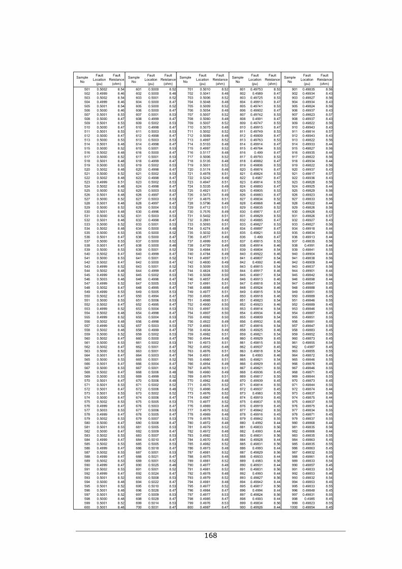
168
Sample No
Fault Location
(pu)
Fault Reistance
(ohm)
Sample No
Fault Location
(pu)
Fault Reistance
(ohm)
Sample No
Fault Location
(pu)
Fault Reistance
(ohm)
Sample No
Fault Location
(pu)
Fault Reistance
(ohm)
Sample No
Fault Location
(pu)
Fault Reistance
(ohm)501 0.5002 8.54 601 0.5000 8.52 701 0.5010 8.52 801 0.49753 8.53 901 0.49835 8.56502 0.4999 8.46 602 0.5000 8.48 702 0.5041 8.48 802 0.4989 8.47 902 0.49934 8.43503 0.5002 8.54 603 0.5001 8.52 703 0.5006 8.52 803 0.49725 8.53 903 0.49827 8.56504 0.4999 8.46 604 0.5000 8.47 704 0.5048 8.48 804 0.49913 8.47 904 0.49934 8.43505 0.5001 8.54 605 0.5000 8.52 705 0.5009 8.52 805 0.49741 8.53 905 0.49824 8.56506 0.5000 8.46 606 0.5000 8.47 706 0.5054 8.48 806 0.49902 8.47 906 0.49937 8.43507 0.5001 8.53 607 0.5001 8.53 707 0.5007 8.52 807 0.49742 8.53 907 0.49823 8.57508 0.5000 8.47 608 0.4999 8.47 708 0.5060 8.48 808 0.4991 8.47 908 0.49937 8.43509 0.5001 8.53 609 0.5002 8.53 709 0.5007 8.52 809 0.49747 8.53 909 0.49822 8.56510 0.5000 8.47 610 0.4998 8.47 710 0.5075 8.48 810 0.49915 8.47 910 0.49943 8.43511 0.5001 8.53 611 0.5003 8.53 711 0.5002 8.52 811 0.49749 8.53 911 0.49814 8.57512 0.5000 8.47 612 0.4998 8.47 712 0.5089 8.48 812 0.49909 8.47 912 0.49943 8.43513 0.5000 8.53 613 0.5003 8.53 713 0.4997 8.52 813 0.49763 8.53 913 0.49822 8.56514 0.5001 8.48 614 0.4998 8.47 714 0.5103 8.48 814 0.49914 8.47 914 0.49933 8.44515 0.5000 8.52 615 0.5001 8.53 715 0.4997 8.52 815 0.49764 8.53 915 0.49827 8.56516 0.5002 8.48 616 0.5000 8.47 716 0.5117 8.48 816 0.499 8.47 916 0.49935 8.44517 0.5000 8.52 617 0.5001 8.53 717 0.5006 8.52 817 0.49793 8.53 917 0.49822 8.56518 0.5001 8.48 618 0.4999 8.47 718 0.5135 8.48 818 0.49882 8.47 918 0.49934 8.44519 0.5000 8.52 619 0.5002 8.53 719 0.5001 8.52 819 0.49806 8.53 919 0.49822 8.56520 0.5002 8.48 620 0.4998 8.47 720 0.5174 8.48 820 0.49874 8.47 920 0.49937 8.43521 0.5000 8.52 621 0.5002 8.53 721 0.4978 8.51 821 0.49824 8.53 921 0.49817 8.57522 0.5002 8.48 622 0.4998 8.47 722 0.5242 8.49 822 0.4987 8.47 922 0.49936 8.43523 0.4999 8.51 623 0.5002 8.53 723 0.4947 8.51 823 0.49814 8.53 923 0.49828 8.56524 0.5002 8.48 624 0.4998 8.47 724 0.5335 8.49 824 0.49893 8.47 924 0.49925 8.44525 0.5000 8.52 625 0.5003 8.53 725 0.4921 8.51 825 0.49805 8.53 925 0.49829 8.56526 0.5001 8.48 626 0.4997 8.47 726 0.5473 8.49 826 0.49883 8.47 926 0.49923 8.44527 0.5000 8.52 627 0.5003 8.53 727 0.4875 8.51 827 0.49834 8.52 927 0.49833 8.56528 0.5001 8.48 628 0.4997 8.47 728 0.5796 8.49 828 0.49868 8.48 928 0.49922 8.44529 0.5000 8.52 629 0.5004 8.53 729 0.4712 8.51 829 0.49835 8.52 929 0.49826 8.56530 0.5001 8.48 630 0.4996 8.47 730 0.7576 8.49 830 0.49877 8.47 930 0.49926 8.43531 0.5000 8.52 631 0.5003 8.53 731 0.5402 8.51 831 0.49829 8.53 931 0.49826 8.57532 0.5001 8.48 632 0.4998 8.47 732 0.2861 8.49 832 0.49885 8.47 932 0.49927 8.43533 0.5000 8.52 633 0.5001 8.53 733 0.5093 8.51 833 0.49827 8.53 933 0.49827 8.56534 0.5002 8.48 634 0.5000 8.48 734 0.4274 8.49 834 0.49897 8.47 934 0.49918 8.44535 0.5000 8.53 635 0.5000 8.52 735 0.5032 8.51 835 0.49821 8.53 935 0.49834 8.56536 0.5001 8.47 636 0.5000 8.47 736 0.4577 8.49 836 0.499 8.47 936 0.49913 8.44537 0.5000 8.53 637 0.5000 8.52 737 0.4999 8.51 837 0.49815 8.53 937 0.49835 8.56538 0.5001 8.47 638 0.5000 8.48 738 0.4709 8.49 838 0.49914 8.46 938 0.4991 8.44539 0.5000 8.53 639 0.5001 8.52 739 0.4984 8.51 839 0.49804 8.54 939 0.49841 8.55540 0.5002 8.47 640 0.4999 8.47 740 0.4784 8.49 840 0.49922 8.46 940 0.49904 8.44541 0.5000 8.53 641 0.5001 8.52 741 0.4997 8.51 841 0.49807 8.54 941 0.49838 8.56542 0.5002 8.47 642 0.5000 8.47 742 0.4800 8.49 842 0.4992 8.46 942 0.49909 8.44543 0.4999 8.52 643 0.5001 8.52 743 0.5009 8.50 843 0.49815 8.54 943 0.49837 8.56544 0.5002 8.48 644 0.4999 8.47 744 0.4824 8.50 844 0.49917 8.46 944 0.49901 8.44545 0.4999 8.52 645 0.5002 8.53 745 0.5008 8.50 845 0.49817 8.54 945 0.49842 8.56546 0.5003 8.48 646 0.4996 8.47 746 0.4857 8.49 846 0.49913 8.46 946 0.49898 8.44547 0.4999 8.52 647 0.5005 8.53 747 0.4991 8.51 847 0.49818 8.54 947 0.49847 8.55548 0.5002 8.47 648 0.4995 8.47 748 0.4888 8.49 848 0.49924 8.46 948 0.49888 8.45549 0.4999 8.53 649 0.5005 8.53 749 0.4977 8.51 849 0.49815 8.54 949 0.49851 8.55550 0.5002 8.47 650 0.4994 8.47 750 0.4905 8.49 850 0.49918 8.46 950 0.49889 8.45551 0.5000 8.53 651 0.5006 8.53 751 0.4988 8.51 851 0.49823 8.54 951 0.49846 8.55552 0.5002 8.47 652 0.4995 8.47 752 0.4900 8.50 852 0.49923 8.46 952 0.49889 8.45553 0.4999 8.52 653 0.5004 8.53 753 0.4997 8.50 853 0.49814 8.54 953 0.49846 8.55554 0.5002 8.48 654 0.4998 8.47 754 0.4907 8.50 854 0.49934 8.46 954 0.49887 8.45555 0.4999 8.52 655 0.5004 8.53 755 0.4992 8.50 855 0.49809 8.54 955 0.49851 8.55556 0.5002 8.48 656 0.4998 8.47 756 0.4922 8.49 856 0.49932 8.46 956 0.49881 8.45557 0.4999 8.52 657 0.5003 8.53 757 0.4983 8.51 857 0.49816 8.54 957 0.49847 8.55558 0.5002 8.48 658 0.4999 8.47 758 0.4934 8.49 858 0.49925 8.46 958 0.49883 8.45559 0.5000 8.52 659 0.5002 8.53 759 0.4982 8.51 859 0.49821 8.54 959 0.49852 8.55560 0.5002 8.47 660 0.5000 8.47 760 0.4944 8.49 860 0.49929 8.45 960 0.49873 8.45561 0.5000 8.53 661 0.5002 8.53 761 0.4973 8.51 861 0.49815 8.55 961 0.49855 8.54562 0.5002 8.47 662 0.5001 8.47 762 0.4952 8.48 862 0.49937 8.45 962 0.4987 8.45563 0.5000 8.52 663 0.5001 8.52 763 0.4976 8.51 863 0.49818 8.54 963 0.49855 8.55564 0.5001 8.47 664 0.5003 8.47 764 0.4951 8.49 864 0.4993 8.46 964 0.49872 8.45565 0.5000 8.53 665 0.5001 8.52 765 0.4980 8.51 865 0.49821 8.54 965 0.49846 8.55566 0.5001 8.47 666 0.5004 8.47 766 0.4954 8.49 866 0.49929 8.45 966 0.49876 8.45567 0.5000 8.53 667 0.5001 8.52 767 0.4976 8.51 867 0.49821 8.55 967 0.49846 8.55568 0.5002 8.47 668 0.5006 8.48 768 0.4960 8.49 868 0.49936 8.45 968 0.49871 8.45569 0.5000 8.53 669 0.4999 8.52 769 0.4979 8.51 869 0.49817 8.55 969 0.49844 8.55570 0.5001 8.47 670 0.5006 8.48 770 0.4962 8.48 870 0.49939 8.45 970 0.49873 8.45571 0.5001 8.53 671 0.5002 8.52 771 0.4975 8.52 871 0.49814 8.55 971 0.49844 8.55572 0.5001 8.47 672 0.5006 8.48 772 0.4966 8.48 872 0.49937 8.45 972 0.49874 8.44573 0.5001 8.53 673 0.5002 8.52 773 0.4976 8.52 873 0.4983 8.55 973 0.49837 8.56574 0.5000 8.47 674 0.5006 8.47 774 0.4967 8.48 874 0.49919 8.45 974 0.49875 8.44575 0.5002 8.53 675 0.5005 8.53 775 0.4977 8.52 875 0.49837 8.55 975 0.49837 8.55576 0.4999 8.47 676 0.5003 8.47 776 0.4969 8.48 876 0.49919 8.45 976 0.49875 8.44577 0.5003 8.53 677 0.5006 8.53 777 0.4979 8.52 877 0.49842 8.55 977 0.49834 8.55578 0.4999 8.47 678 0.5005 8.47 778 0.4969 8.48 878 0.49916 8.45 978 0.49871 8.45579 0.5002 8.53 679 0.5007 8.53 779 0.4978 8.52 879 0.49842 8.55 979 0.49837 8.55580 0.5000 8.47 680 0.5008 8.47 780 0.4972 8.48 880 0.4992 8.44 980 0.49868 8.44581 0.5001 8.53 681 0.5005 8.53 781 0.4979 8.52 881 0.49833 8.56 981 0.49835 8.56582 0.5000 8.47 682 0.5009 8.47 782 0.4972 8.48 882 0.4993 8.44 982 0.49866 8.44583 0.5002 8.53 683 0.5007 8.53 783 0.4982 8.52 883 0.49831 8.56 983 0.49835 8.55584 0.4999 8.47 684 0.5010 8.47 784 0.4970 8.48 884 0.49928 8.44 984 0.49863 8.45585 0.5002 8.53 685 0.5005 8.53 785 0.4982 8.52 885 0.49831 8.56 985 0.49835 8.55586 0.4999 8.47 686 0.5018 8.47 786 0.4973 8.48 886 0.4993 8.44 986 0.49863 8.45587 0.5002 8.53 687 0.5001 8.53 787 0.4981 8.52 887 0.49829 8.56 987 0.49832 8.55588 0.4999 8.47 688 0.5021 8.47 788 0.4975 8.48 888 0.49933 8.44 988 0.49861 8.45589 0.5002 8.53 689 0.5001 8.52 789 0.4981 8.52 889 0.4983 8.56 989 0.49833 8.54590 0.4999 8.47 690 0.5025 8.48 790 0.4977 8.48 890 0.49931 8.44 990 0.49857 8.45591 0.5002 8.53 691 0.5001 8.52 791 0.4981 8.52 891 0.49831 8.56 991 0.49833 8.54592 0.4999 8.47 692 0.5024 8.47 792 0.4978 8.48 892 0.4993 8.44 992 0.49853 8.46593 0.5001 8.52 693 0.5008 8.53 793 0.4979 8.52 893 0.49827 8.56 993 0.49832 8.54594 0.5000 8.48 694 0.5022 8.47 794 0.4981 8.48 894 0.49942 8.44 994 0.49853 8.45595 0.5001 8.52 695 0.5010 8.53 795 0.4977 8.52 895 0.49817 8.56 995 0.49833 8.55596 0.5001 8.48 696 0.5026 8.47 796 0.4984 8.47 896 0.4994 8.44 996 0.49848 8.45597 0.5001 8.52 697 0.5009 8.53 797 0.4977 8.53 897 0.49824 8.56 997 0.49831 8.55598 0.5000 8.48 698 0.5028 8.47 798 0.4985 8.47 898 0.4993 8.44 998 0.4985 8.45599 0.5001 8.52 699 0.5014 8.53 799 0.4976 8.53 899 0.49834 8.56 999 0.49823 8.55600 0.5001 8.48 700 0.5031 8.47 800 0.4987 8.47 900 0.49926 8.44 1000 0.49854 8.45

Appendix B
PhD publications presented during his PhD research project are followed.
169
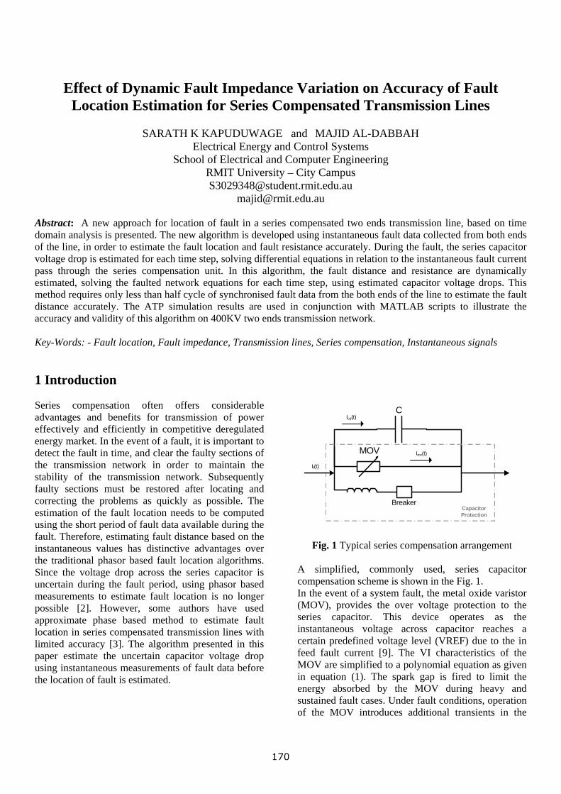
Effect of Dynamic Fault Impedance Variation on Accuracy of Fault Location Estimation for Series Compensated Transmission Lines
SARATH K KAPUDUWAGE and MAJID AL-DABBAH
Electrical Energy and Control Systems School of Electrical and Computer Engineering
RMIT University – City Campus [email protected]
[email protected] Abstract: A new approach for location of fault in a series compensated two ends transmission line, based on time domain analysis is presented. The new algorithm is developed using instantaneous fault data collected from both ends of the line, in order to estimate the fault location and fault resistance accurately. During the fault, the series capacitor voltage drop is estimated for each time step, solving differential equations in relation to the instantaneous fault current pass through the series compensation unit. In this algorithm, the fault distance and resistance are dynamically estimated, solving the faulted network equations for each time step, using estimated capacitor voltage drops. This method requires only less than half cycle of synchronised fault data from the both ends of the line to estimate the fault distance accurately. The ATP simulation results are used in conjunction with MATLAB scripts to illustrate the accuracy and validity of this algorithm on 400KV two ends transmission network. Key-Words: - Fault location, Fault impedance, Transmission lines, Series compensation, Instantaneous signals
1 Introduction Series compensation often offers considerable advantages and benefits for transmission of power effectively and efficiently in competitive deregulated energy market. In the event of a fault, it is important to detect the fault in time, and clear the faulty sections of the transmission network in order to maintain the stability of the transmission network. Subsequently faulty sections must be restored after locating and correcting the problems as quickly as possible. The estimation of the fault location needs to be computed using the short period of fault data available during the fault. Therefore, estimating fault distance based on the instantaneous values has distinctive advantages over the traditional phasor based fault location algorithms. Since the voltage drop across the series capacitor is uncertain during the fault period, using phasor based measurements to estimate fault location is no longer possible [2]. However, some authors have used approximate phase based method to estimate fault location in series compensated transmission lines with limited accuracy [3]. The algorithm presented in this paper estimate the uncertain capacitor voltage drop using instantaneous measurements of fault data before the location of fault is estimated.
C
MOV
BreakerCapacitor Protection
If(t)
Icp(t)
Imv(t)
Fig. 1 Typical series compensation arrangement
A simplified, commonly used, series capacitor compensation scheme is shown in the Fig. 1. In the event of a system fault, the metal oxide varistor (MOV), provides the over voltage protection to the series capacitor. This device operates as the instantaneous voltage across capacitor reaches a certain predefined voltage level (VREF) due to the in feed fault current [9]. The VI characteristics of the MOV are simplified to a polynomial equation as given in equation (1). The spark gap is fired to limit the energy absorbed by the MOV during heavy and sustained fault cases. Under fault conditions, operation of the MOV introduces additional transients in the
170
transmission network, which will render the location of fault difficult to estimate accurately [5]. Since the proposed algorithm is based on the measurements of instantaneous values, the transient presence during the operation of the MOV will have fewer effects in estimation of the fault location. The algorithm presented in this paper is developed for a two-end transmission line with series compensation is located at the centre of the line. This algorithm uses instantaneous measurements of synchronised fault data from both ends of the line for very short duration to estimate fault location accurately. In the case of long transmission line, the synchronised fault data measurements can be accurately recorded with absolute time references, using Global Positioning System (GPS). Application of high performance GPS recorders is not expensive and easily available nowadays, and can be used to record signals up to the accuracy of 100ns at 95% probability [10]. Fault measurement samples from both ends can be synchronised, with very high accuracy using more intelligent type of master clock [10]. If instantaneous values of voltages and currents from both ends of the transmission line are known, fault equation can be solved estimating distance to fault (x) and fault resistance (rf) for each time step. It was observed that the sampling rate of measurements needs minimum of 100 kHz to achieve the fault location accuracy stated in this paper. A 400KV, 300km two ends transmission line was modelled and simulated using ATP software and instantaneous fault signals were recorded to evaluate the accuracy of this algorithm. The sampling rate of the measurements was set at 100 KHz. The algorithm for the estimation of fault location and resistance was developed using MATLAB script language. Simulation of numerous types of fault cases have been conducted with many variations and the recorded data has been input in algorithm to compute the fault location and resistance for each time step. The result arrays have been further processed numerically to obtain the average values of the fault distance and resistance. The results indicate that the average fault location error estimated using this algorithm is below 0.2%. A new, robust and accurate method, for estimating the location of faults of a series compensated transmission line using time domain signals is introduced in this paper, with a brief introduction to the associated basic problems. Section 2 describes the basic operation of the series compensation and how the voltage drop is estimated across the series compensation using sample data, and applied to the new algorithm. System
configuration of the transmission model and the development of the new algorithm are given in Section 3 and 4. Subsequently testing of new algorithm using ATP model is described in Section 5. Finally the evaluation of the results and conclusions are followed in Sections 6 and 7. 2. Series Compensation Model Fig. 1 shows the typical configuration of the series compensation device, and its basic protection mechanism. The complicity of developing an accurate method of computing the location fault is heavily dependent on the protection devices incorporated in series compensation. The MOV conducts immediately after the capacitor instantaneous voltage drop across the capacitor exceeds a certain voltage level (VREF). The VI characteristics of the MOV can be expressed by a nonlinear equation:
⎟⎟⎠
⎞⎜⎜⎝
⎛=
VREFp V
ICP
q
MOV * (1) Where p and VREF are the reference quantities of the MOV and typically, q is in the order of 20 to 30 [11]. During heavy and sustaining fault currents, the MOV exceeds its maximum energy absorption limit. The spark gap is fired to protect this device of being over burdened as shown in Fig. 1. The operating level of the spark gap is derived from the quantity and duration of the fault current continue to pass through the MOV. If the fault current is I f under any operational conditions, other than the spark gap is in operation, it can be expressed in terms of:
)()()( tI mvtI cptI f += (2) where I CP and I MV are capacitor current and MOV current which flow through the series compensation circuit at a given time t. Under normal load conditions, line current Il = I cp and I mv = 0. Under fault conditions, over voltage protection operates, when fault current exceeds 0.98Ipu, where I pu is defined with reference to the capacitor currents. (I pu = I cp / I pr) I pr is the capacitor protective level current [2]. Therefore, faulted SCU voltage drop needs to be estimated considering these conditions. 2.1 MOV is not conducting If the fault current is known, the voltage drop across the capacitor can be expressed by instantaneous values:
dttC
Ttt tTt Fcpcp iVV )(1)()( ∫ −+−= (3)
171
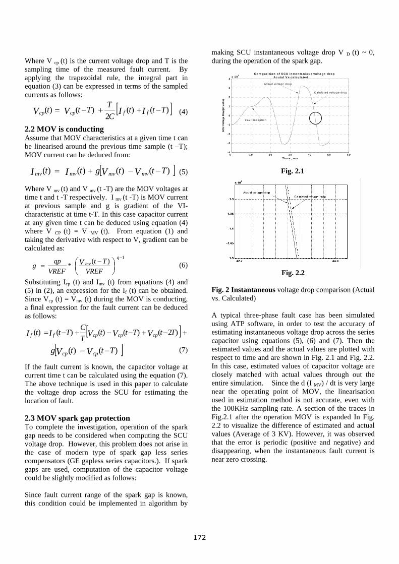
Where V cp (t) is the current voltage drop and T is the sampling time of the measured fault current. By applying the trapezoidal rule, the integral part in equation (3) can be expressed in terms of the sampled currents as follows:
0 1 0 2 0 3 0 4 0 5 0 6 0-4
-3
-2
-1
0
1
2
3
4x 1 0 5
T im e , m s
SCU
Vol
tage
Dro
p(in
Vol
ts)
C o m p a risio n o f S C U in sta n ta n io u s vo lta g e d ro p A cu ta l V s ca lcu la te d
Fa u l t In ce p tio n
Ac tu a l vo lta g e d ro p
C a lu la te d vo lta g e d ro p
(4)
2.2 MOV is conducting Assume that MOV characteristics at a given time t can be linearised around the previous time sample (t –T); MOV current can be deduced from:
(5) Where V mv (t) and V mv (t -T) are the MOV voltages at time t and t -T respectively. I mv (t -T) is MOV current at previous sample and g is gradient of the VI-characteristic at time t-T. In this case capacitor current at any given time t can be deduced using equation (4) where V CP (t) = V MV (t). From equation (1) and taking the derivative with respect to V, gradient can be calculated as:
(6) Substituting Icp (t) and Imv (t) from equations (4) and (5) in (2), an expression for the If (t) can be obtained. Since Vcp (t) = Vmv (t) during the MOV is conducting, a final expression for the fault current can be deduced as follows:
(7) If the fault current is known, the capacitor voltage at current time t can be calculated using the equation (7). The above technique is used in this paper to calculate the voltage drop across the SCU for estimating the location of fault. 2.3 MOV spark gap protection To complete the investigation, operation of the spark gap needs to be considered when computing the SCU voltage drop. However, this problem does not arise in the case of modern type of spark gap less series compensators (GE gapless series capacitors.). If spark gaps are used, computation of the capacitor voltage could be slightly modified as follows: Since fault current range of the spark gap is known, this condition could be implemented in algorithm by
making SCU instantaneous voltage drop V D (t) ~ 0, during the operation of the spark gap.
[ ])()(2
)()( TttCTTtt IIVV ffcpcp −++−=
[ ])()()()( Tttgtt VVII mvmvmvmv −−+= Fig. 2.1
Fig. 2.2
⎟⎠⎞
⎜⎝⎛ −
=−
VREFTt
VREFqpg V mv
q)(*1
Fig. 2 Instantaneous voltage drop comparison (Actual vs. Calculated) A typical three-phase fault case has been simulated using ATP software, in order to test the accuracy of estimating instantaneous voltage drop across the series capacitor using equations (5), (6) and (7). Then the estimated values and the actual values are plotted with respect to time and are shown in Fig. 2.1 and Fig. 2.2. In this case, estimated values of capacitor voltage are closely matched with actual values through out the entire simulation. Since the d (I MV) / dt is very large near the operating point of MOV, the linearisation used in estimation method is not accurate, even with the 100KHz sampling rate. A section of the traces in Fig.2.1 after the operation MOV is expanded In Fig. 2.2 to visualize the difference of estimated and actual values (Average of 3 KV). However, it was observed that the error is periodic (positive and negative) and disappearing, when the instantaneous fault current is near zero crossing.
[ ] +−+−−+−= )2()()()()( TtTttTCTtt VVVI
I cpcpcpff
[ ])()( Tttg VV cpcp −−
172

3. System Configuration Fig. 3 shows a single line diagram of a basic two-end transmission network with a series compensation unit (SCU) is, located at the center of the line. It was considered that having SCU far away from the fault locator (150 km), direct measuring of the instantaneous SCU voltage drop with absolute time reference will be more difficult and not cost effective, and hence needs to be computed before estimating the fault location. The fault location algorithm is developed considering fault locations before and after the SCU. As in Fig. 3 fault locator (FL) is in the local station (S). At the each end of the transmission line, digital fault recorders are used to measure and record instantaneous fault data in the event of a fault. The GPS receivers are used for accurate synchronisation of recording devices. Fault data with accurate time references from the remote end are sent to the fault locator via communication links. It was observed that accurate synchronisation of fault data from local and remote ends are critical for accurate estimation of fault location using proposed algorithm. However, fault data mismatch has been tested and results are briefly discussed in section 6. Fig. 3 Basic two-end transmission network In general three phase voltage sources can be expressed in matrix form [2];
(8) Where ES is the local end voltage source and a, b and c are referred to three phases. Consider fault distance is x pu from the local end. Transmission line impedance (ZL) can be written in matrix form:
(9)
Where Z Lss and Z Lmm are self and mutual impedances of the transmission line. It was assumed line is completely transposed and therefore self and mutual impedances are identical for all three phases. 4. Development of the new algorithm 4.1 fault location Let us consider the configuration of a two terminal transmission line as shown in Fig. 3. Assume the fault occurs on the line at F1, x kilometres from the local bus, prior to SCU. If the voltage and current at the local bus and remote buses are V s, I s, V R and I R respectively, then the network equation of the faulted system can be written in matrix form: [ ] [ ][ ] [ ] [ ] [ ][ ]IVVIV RLRDSLs ZxZx )1( −−=−− (10)
Where [V D] is the voltage drop across the series compensation unit. If the fault occurs on the line at F2, after SCU, the fault equation could be modified as follows: [ ] [ ][ ] [ ] [ ][ ] [ ]VIZxVIZxV DRLRSLs −−−=− )1( (11)
In both cases, capacitor instantaneous voltage drops can be computed either using I R or I S.
(1-x)ZL
MOV
C
VF
F2
IF
F1
Station R
ES
Station S
ZS xZL
IS
VS
FLZR
ER
IR
VR
GPSReceiver
DFR
GPSReceiver
DFRCoomunication lines
[ZL][IS] instantaneous voltage drops can be computed using differential equation in the time domain and takes the form:
⎥⎥⎥
⎦
⎤
⎢⎢⎢
⎣
⎡
⎥⎥⎥
⎦
⎤
⎢⎢⎢
⎣
⎡+⎥⎥⎥
⎦
⎤
⎢⎢⎢
⎣
⎡
⎥⎥⎥
⎦
⎤
⎢⎢⎢
⎣
⎡
dtdtdt
dI
dI
dI
XMM
MXM
MMX
R
I
I
R
R
R
Sc
Sb
Sa
LcLcbLca
LbcLbLba
LacLabLa
Sc
Sb
Sa
Lc
Lb
La
///
(12) Where RL and XL are the line total resistance and self inductance. ML is the mutual inductance between phases. [ZL][IR] also can be computed similarly and both are of 3 x 1 matrices.
[ ]EEEE scsbsaT
S =
Knowing capacitor voltage drop [VD], equation (10) and (11) can be solved to compute the fault location x for each time sampling step. 4.2 selection method Since the location of the fault is not known prior to the estimation of fault distance, results obtained from both equations are not valid. To solve this problem, first compute the fault location using equation (10) and (11). Finding the correct result can be argued as follows:
[ ]⎥⎥⎥
⎦
⎤
⎢⎢⎢
⎣
⎡=
ZZZ
ZZZ
ZZZ
LssLmmLmm
LmmLssLmm
LmmLmmLss
LZ
173
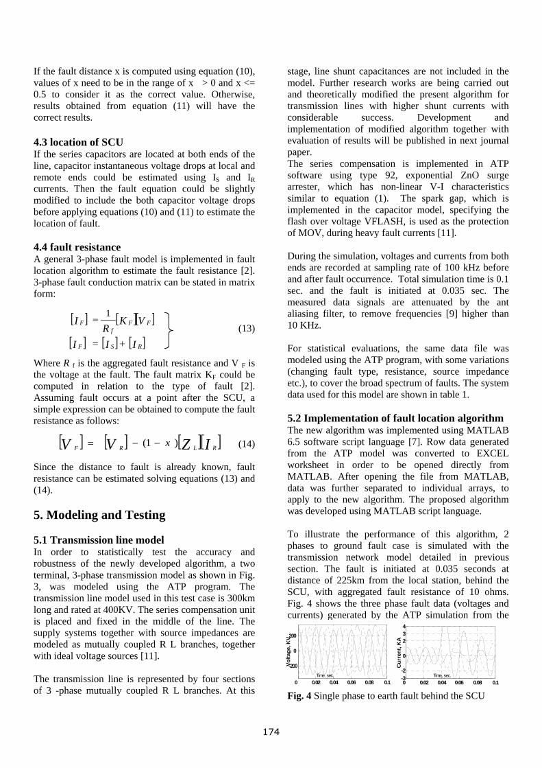
If the fault distance x is computed using equation (10), values of x need to be in the range of x > 0 and x <= 0.5 to consider it as the correct value. Otherwise, results obtained from equation (11) will have the correct results. 4.3 location of SCU If the series capacitors are located at both ends of the line, capacitor instantaneous voltage drops at local and remote ends could be estimated using IS and IR currents. Then the fault equation could be slightly modified to include the both capacitor voltage drops before applying equations (10) and (11) to estimate the location of fault. 4.4 fault resistance A general 3-phase fault model is implemented in fault location algorithm to estimate the fault resistance [2]. 3-phase fault conduction matrix can be stated in matrix form:
(13) Where R f is the aggregated fault resistance and V F is the voltage at the fault. The fault matrix KF could be computed in relation to the type of fault [2]. Assuming fault occurs at a point after the SCU, a simple expression can be obtained to compute the fault resistance as follows:
(14) Since the distance to fault is already known, fault resistance can be estimated solving equations (13) and (14). 5. Modeling and Testing 5.1 Transmission line model In order to statistically test the accuracy and robustness of the newly developed algorithm, a two terminal, 3-phase transmission model as shown in Fig. 3, was modeled using the ATP program. The transmission line model used in this test case is 300km long and rated at 400KV. The series compensation unit is placed and fixed in the middle of the line. The supply systems together with source impedances are modeled as mutually coupled R L branches, together with ideal voltage sources [11]. The transmission line is represented by four sections of 3 -phase mutually coupled R L branches. At this
stage, line shunt capacitances are not included in the model. Further research works are being carried out and theoretically modified the present algorithm for transmission lines with higher shunt currents with considerable success. Development and implementation of modified algorithm together with evaluation of results will be published in next journal paper. The series compensation is implemented in ATP software using type 92, exponential ZnO surge arrester, which has non-linear V-I characteristics similar to equation (1). The spark gap, which is implemented in the capacitor model, specifying the flash over voltage VFLASH, is used as the protection of MOV, during heavy fault currents [11]. During the simulation, voltages and currents from both ends are recorded at sampling rate of 100 kHz before and after fault occurrence. Total simulation time is 0.1 sec. and the fault is initiated at 0.035 sec. The measured data signals are attenuated by the ant aliasing filter, to remove frequencies [9] higher than 10 KHz. [ ] [ ][ ]
[ ] [ ] [ ]III
VKR
I
RSF
FFf
F
+=
=1
For statistical evaluations, the same data file was modeled using the ATP program, with some variations (changing fault type, resistance, source impedance etc.), to cover the broad spectrum of faults. The system data used for this model are shown in table 1. 5.2 Implementation of fault location algorithm The new algorithm was implemented using MATLAB 6.5 software script language [7]. Row data generated from the ATP model was converted to EXCEL worksheet in order to be opened directly from MATLAB. After opening the file from MATLAB, data was further separated to individual arrays, to apply to the new algorithm. The proposed algorithm was developed using MATLAB script language.
[ ] [ ] [ ][ ]IZVV RLRFx )1( −−=
To illustrate the performance of this algorithm, 2 phases to ground fault case is simulated with the transmission network model detailed in previous section. The fault is initiated at 0.035 seconds at distance of 225km from the local station, behind the SCU, with aggregated fault resistance of 10 ohms. Fig. 4 shows the three phase fault data (voltages and currents) generated by the ATP simulation from the local station S. 0 0.02 0.04 0.06 0.08 0.1
-200
0
0 0.02 0.04 0.06 0.08 0.1-3-2
0
234
Cur
rent
, KA
Time, sec.
Fig. 4 Single phase to earth fault behind the SCU
200
Volta
ge, K
V
Time, sec.
174
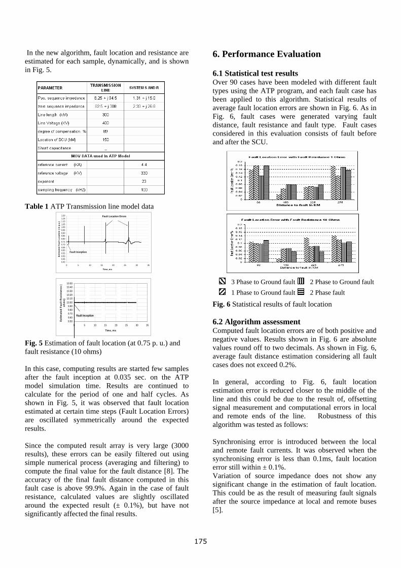
In the new algorithm, fault location and resistance are estimated for each sample, dynamically, and is shown in Fig. 5. Table 1 ATP Transmission line model data Fig. 5 Estimation of fault location (at 0.75 p. u.) and fault resistance (10 ohms) In this case, computing results are started few samples after the fault inception at 0.035 sec. on the ATP model simulation time. Results are continued to calculate for the period of one and half cycles. As shown in Fig. 5, it was observed that fault location estimated at certain time steps (Fault Location Errors) are oscillated symmetrically around the expected results. Since the computed result array is very large (3000 results), these errors can be easily filtered out using simple numerical process (averaging and filtering) to compute the final value for the fault distance [8]. The accuracy of the final fault distance computed in this fault case is above 99.9%. Again in the case of fault resistance, calculated values are slightly oscillated around the expected result (± 0.1%), but have not significantly affected the final results.
6. Performance Evaluation 6.1 Statistical test results Over 90 cases have been modeled with different fault types using the ATP program, and each fault case has been applied to this algorithm. Statistical results of average fault location errors are shown in Fig. 6. As in Fig. 6, fault cases were generated varying fault distance, fault resistance and fault type. Fault cases considered in this evaluation consists of fault before and after the SCU.
0.400.450.500.550.600.650.700.750.800.850.900.951.001.051.101.151.20
0 5 10 15 20 25 30 35
Time, ms
Estim
ated
Fau
lt Lo
catio
n ( i
n p.
u.)
Fault Inception
Fault Location Errors Fig. 6 Statistical results of fault location 6.2 Algorithm assessment Computed fault location errors are of both positive and negative values. Results shown in Fig. 6 are absolute values round off to two decimals. As shown in Fig. 6, average fault distance estimation considering all fault cases does not exceed 0.2%. In general, according to Fig. 6, fault location estimation error is reduced closer to the middle of the line and this could be due to the result of, offsetting signal measurement and computational errors in local and remote ends of the line. Robustness of this algorithm was tested as follows: Synchronising error is introduced between the local and remote fault currents. It was observed when the synchronising error is less than 0.1ms, fault location error still within ± 0.1%. Variation of source impedance does not show any significant change in the estimation of fault location. This could be as the result of measuring fault signals after the source impedance at local and remote buses [5].
9.509.609.709.809.90
10.0010.1010.2010.3010.4010.50
0 5 10 15 20 25 30 35
Time, ms
Estim
ated
Fau
lt R
esis
tanc
e (
ohm
s)
Fault Inception
3 Phase to Ground fault 1 Phase to Ground fault
2 Phase to Ground fault2 Phase fault
175
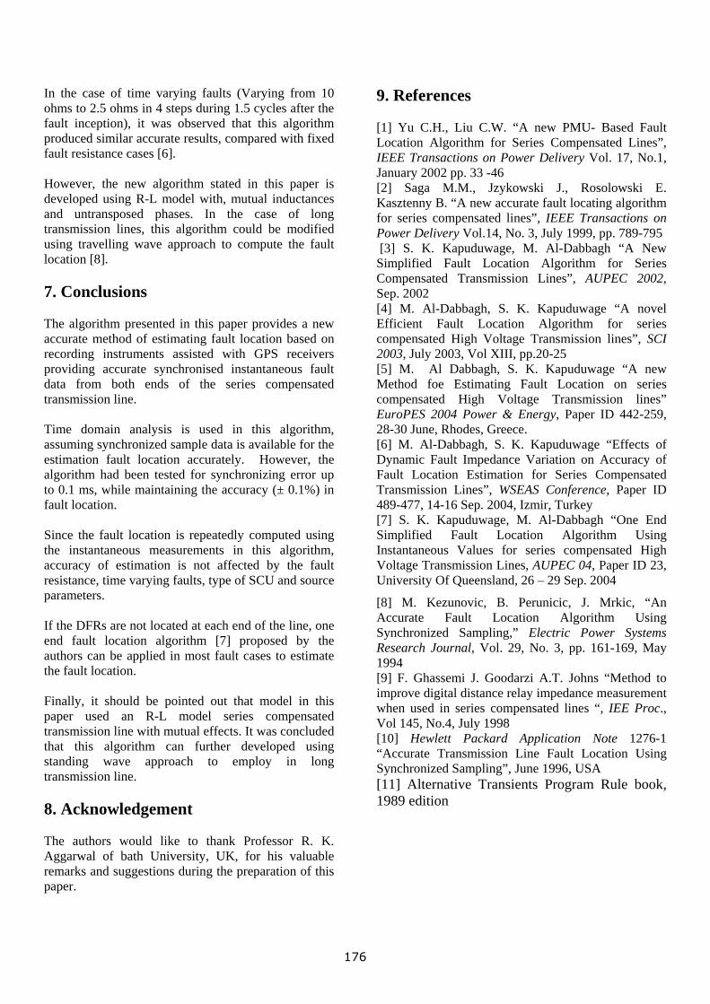
In the case of time varying faults (Varying from 10 ohms to 2.5 ohms in 4 steps during 1.5 cycles after the fault inception), it was observed that this algorithm produced similar accurate results, compared with fixed fault resistance cases [6]. However, the new algorithm stated in this paper is developed using R-L model with, mutual inductances and untransposed phases. In the case of long transmission lines, this algorithm could be modified using travelling wave approach to compute the fault location [8]. 7. Conclusions The algorithm presented in this paper provides a new accurate method of estimating fault location based on recording instruments assisted with GPS receivers providing accurate synchronised instantaneous fault data from both ends of the series compensated transmission line. Time domain analysis is used in this algorithm, assuming synchronized sample data is available for the estimation fault location accurately. However, the algorithm had been tested for synchronizing error up to 0.1 ms, while maintaining the accuracy (± 0.1%) in fault location. Since the fault location is repeatedly computed using the instantaneous measurements in this algorithm, accuracy of estimation is not affected by the fault resistance, time varying faults, type of SCU and source parameters. If the DFRs are not located at each end of the line, one end fault location algorithm [7] proposed by the authors can be applied in most fault cases to estimate the fault location. Finally, it should be pointed out that model in this paper used an R-L model series compensated transmission line with mutual effects. It was concluded that this algorithm can further developed using standing wave approach to employ in long transmission line. 8. Acknowledgement The authors would like to thank Professor R. K. Aggarwal of bath University, UK, for his valuable remarks and suggestions during the preparation of this paper.
9. References [1] Yu C.H., Liu C.W. “A new PMU- Based Fault Location Algorithm for Series Compensated Lines”, IEEE Transactions on Power Delivery Vol. 17, No.1, January 2002 pp. 33 -46 [2] Saga M.M., Jzykowski J., Rosolowski E. Kasztenny B. “A new accurate fault locating algorithm for series compensated lines”, IEEE Transactions on Power Delivery Vol.14, No. 3, July 1999, pp. 789-795 [3] S. K. Kapuduwage, M. Al-Dabbagh “A New Simplified Fault Location Algorithm for Series Compensated Transmission Lines”, AUPEC 2002, Sep. 2002 [4] M. Al-Dabbagh, S. K. Kapuduwage “A novel Efficient Fault Location Algorithm for series compensated High Voltage Transmission lines”, SCI 2003, July 2003, Vol XIII, pp.20-25 [5] M. Al Dabbagh, S. K. Kapuduwage “A new Method foe Estimating Fault Location on series compensated High Voltage Transmission lines” EuroPES 2004 Power & Energy, Paper ID 442-259, 28-30 June, Rhodes, Greece. [6] M. Al-Dabbagh, S. K. Kapuduwage “Effects of Dynamic Fault Impedance Variation on Accuracy of Fault Location Estimation for Series Compensated Transmission Lines”, WSEAS Conference, Paper ID 489-477, 14-16 Sep. 2004, Izmir, Turkey [7] S. K. Kapuduwage, M. Al-Dabbagh “One End Simplified Fault Location Algorithm Using Instantaneous Values for series compensated High Voltage Transmission Lines, AUPEC 04, Paper ID 23, University Of Queensland, 26 – 29 Sep. 2004
[8] M. Kezunovic, B. Perunicic, J. Mrkic, “An Accurate Fault Location Algorithm Using Synchronized Sampling,” Electric Power Systems Research Journal, Vol. 29, No. 3, pp. 161-169, May 1994 [9] F. Ghassemi J. Goodarzi A.T. Johns “Method to improve digital distance relay impedance measurement when used in series compensated lines “, IEE Proc., Vol 145, No.4, July 1998 [10] Hewlett Packard Application Note 1276-1 “Accurate Transmission Line Fault Location Using Synchronized Sampling”, June 1996, USA [11] Alternative Transients Program Rule book, 1989 edition
176
Using Instantaneous Values for Estimating Fault Locations on series compensated Transmission Lines
Majid Al-Dabbagh and Sarath K. Kapuduwage
Electrical Energy and Control Systems School of Electrical and Computer Engineering
RMIT University, Melbourne, Australia Abstract— Fault location estimation hitherto is based on using the filtered RMS values from both ends of the line. In this paper, a new method for locating faults on series compensated high voltage transmission lines, based on the instantaneous values is proposed. Based on the results achieved with the new algorithm, using instantaneous values, the distance to fault location is estimated very accurately [5]. However, the accuracy of the fault location is limited to the ability to capture data samples before the operation of the MOV. The proposed algorithm incorporates special techniques to avoid the limitation caused by the operation of the MOV. It is formal that although the accuracy of fault location using the algorithm proposed is slightly reduced, but still acceptable. This paper describes the new algorithm and examines its accuracy as compared to other method [5]. Keywords—fault location, series compensated lines, instantaneous values
1. INTRODUCTION The introduction of series capacitors in high voltage transmission lines brought several advantages to power system operations, such as improving power transfer capability, transient stability and damping power system oscillations. Under a fault conditions, the voltage drop across the capacitor can be dangerously high and metal oxide varistor [MOV] is used in parallel with the capacitors to protect them against such conditions. Due to the operation of MOV, which has nonlinear characteristic, fault estimation using impedance measurement techniques can no longer be used to estimate the location of a fault accurately [1, 2]. In order to estimate fault locations accurately, the voltage drop of series compensation unit is required to be computed precisely [7]. However, the existing methods available for such computations induce considerable errors in fault location estimation, due to the complexity of the series compensation units [1]. The proposed algorithm in this paper uses instantaneous measured data from the faulted power network, taking into consideration the operation of MOV, to estimate the voltage drop across the series capacitor accurately. Once the uncertain voltage drop across the capacitor is deducted from the fault equation, fault location can be estimated by calculating the voltage drop across the transmission line. The basic arrangement of series compensation of a transmission line is a series capacitor (C) in parallel with a metal oxide resistor (MOV) is shown in Fig. 1 Under fault conditions, operation of the MOV introduces additional transients in the transmission network, which will render the location of the fault difficult to estimate accurately.
177

C
MOV
BreakerCapacitorProtection
If(t)
Icp(t)
Imv(t)
Fig. 1. Capacitor protection To overcome the above problem, time domain analysis based on the measurement of the instantaneous values [7] has been used in proposed algorithm to estimate the location of fault, considering the effects of transients present during operation of the MOV. In this proposed algorithm, voltage drop of each component in the transmission network is estimated in time steps immediately before and after the fault initiation. Algorithm presented in this paper, conditionally computes the series compensator voltage drop using measured instantaneous values [7], before and after the operation of MOV during a fault condition. When the voltage drop is below the series capacitor protection level [6], current pass through the MOV would be nearly zero. Therefore, the voltage drop is calculated using series capacitive reactance. Otherwise, the voltage drop is computed considering both capacitor and MOV currents. The proposed fault location algorithm has been applied to two-end transmission line, with series compensating device placed at the centre of the line. If voltages and currents from both ends of the transmission are known, fault equations can be solved estimating distance to fault (x) and fault resistance (rf). It was observed that the sampling rate of measurements needs to be at least at 100KHz, to achieve the fault location accuracy stated in this paper. The data generated from a 400KV 300km transmission line model, which is simulated in the ATP program has been used to evaluate the accuracy of this algorithm.. Raw data, from the two substations, measured at a sampling rate of 100kHz. The presented algorithm was tested using sample data collected form numerous types of faults simulated in ATP program. The results indicate that the average fault location error is the range of 99.8% to 99.9%. The error is slightly increased compared to the other method [5] due the effect of operation of the MOV. A new, robust and accurate method, for estimating the location of faults of a series compensated transmission line using time domain signals is introduced in this paper, with a brief introduction to the associated basic problems. Section 2 describes the basic operation of the series compensation and how the voltage drop is estimated across the series compensation using sample data, and applied to the new algorithm. System configuration of the transmission model and the development of the new algorithm are given in Section 3 and 4. Subsequently testing of new algorithm using ATP model is described in Section 5. Performance evaluation of the results and the algorithm assessment are followed in Sections 6 and 7.
178
2. SERIES COMPENSATOR MODEL
Fig. 1 shows the typical configuration of the series compensation device, with its basic protection mechanism. During normal operations, the series capacitor (C) generates leading VARS to compensate some of the VAR consumed by the network. The Metal Oxide Varistor (MOV) is the main protection device, which operates when an over voltage is detected across the capacitor. With a short circuit on the line, the capacitor is subjected to an extremely high voltage, which is controlled by the conduction of MOV. The voltage protection level of MOV (1.5pu to 2.0pu) is determined with reference to the capacitor voltage drop with rated current flowing through it [6]. The VI–characteristics of the MOV can be approximated by a nonlinear equation:
⎟⎠⎞
⎜⎝⎛=
VREFVpi
q
* (1) Where p and VREF are the reference quantities of the MOV and typically q is in the order of 20 to 30 [9]. The Circuit Breaker provides the protection of MOV to limit the absorption energy during operation. As shown in Fig. 1, if the fault current passing through the series compensation unit (SCU) is If, under any operational condition it can be shown that:
If (t) = Icp(t) + Imv(t) (2) where Icp and Imv are the capacitor and MOV currents. Under normal load conditions, line current Il = Icp and Imv = 0. Under fault conditions, MOV begins to conduct when fault current exceeds 0.98Ipu, where Ipu is defined with reference to the capacitor currents. ( Ipu = Icp / Ipr) where Ipr is the capacitor protective level current. Therefore, faulted SCU voltage drop need to be estimated in two ways: A. MOV is not conducting If the fault current is known, the voltage drop across the capacitor can be expressed in terms of instantaneous values:
dttC
Ttt tTt Fcpcp iVV )(1)()( ∫ −+−= (3)
Where Vcp(t) is the current voltage drop, and T is the sampling time of the measured fault current. By applying the Trapezoidal Rule, the integral part in equation (3) can be expressed in terms of the sampled currents as follows:
[ ])()(2
)()( TttCTTtt IIVV ffcpcp −++−= (4)
B. MOV is conducting Assume that MOV characteristics at a given time t can be linearised around the previous time sample ( t –T ), MOV current can be deduced from: [ ])()()()( Tttgtt VVII mvmvmvmv −−+= (5)
179
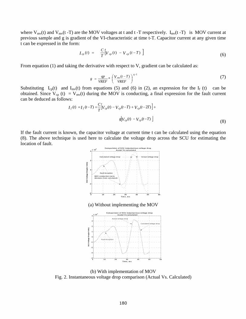
where Vmv(t) and Vmv(t -T) are the MOV voltages at t and t -T respectively. Imv(t -T) is MOV current at previous sample and g is gradient of the VI-characteristic at time t-T. Capacitor current at any given time t can be expressed in the form: [ ])()()( Ttt
TCt VVI cpcpcp −−= (6)
From equation (1) and taking the derivative with respect to V, gradient can be calculated as:
(7) ⎟⎠⎞
⎜⎝⎛ −
=−
VREFTt
VREFqpg V mv
q)(*1
Substituting Icp(t) and Imv(t) from equations (5) and (6) in (2), an expression for the If (t) can be obtained. Since Vcp (t) = Vmv(t) during the MOV is conducting, a final expression for the fault current can be deduced as follows: [ ] +−+−−+−= )2()()()()( TtTtt
TCTtt VVVII cpcpcpff
[ ])()( Tttg VV cpcp −− (8)
If the fault current is known, the capacitor voltage at current time t can be calculated using the equation (8). The above technique is used here to calculate the voltage drop across the SCU for estimating the location of fault.
0 10 20 30 40 50 60-5
-3
0
2
4x 10 5
T im e , m s
SC
U V
olta
ge D
rop(
in V
olts
)
C o m p a risio n o f S CU in sta n ta n io u s vo l ta g e d ro p A cu ta l V s ca lcu la te d
Fa ult Inc e ption
M O V c onduc tion s ta r ts (de via te s from c a lc u la te d)
Ac tua l vo lta ge drop Ca lc u la te d vo lta ge drop
(a) Without implementing the MOV
0 1 0 2 0 3 0 4 0 5 0 6 0-4
-3
-2
-1
0
1
2
3
4x 1 0 5
T im e , m s
SCU
Vol
tage
Dro
p(in
Vol
ts)
C o m p a risio n o f S CU in sta n ta n io u s vo l ta g e d ro p A cu ta l V s ca lcu la te d
Fa u lt In ce p tio n
Ac tu a l vo l ta g e d ro p
C a lu la te d vo lta g e d ro p
(b) With implementation of MOV
Fig. 2. Instantaneous voltage drop comparison (Actual Vs. Calculated)
180

To illustrate the practicability and accuracy of the above method in estimating the voltage drop across the capacitor during a fault, a three-phase fault case has been simulated using the ATP program, and the instantaneous values of SCU voltage drop have been recorded. The above method is used with and without implementing the presence of MOV and estimated the voltage drops across the SCU. The comparison of the instantaneous voltage drop across the SCU; the actual ATP output and values computed by this algorithm are shown in Fig. 2 (a) and (b). It was assumed that there was no load on the network prior to the fault. In Fig. 2 (a), the calculated values follows the actual values, up to the time where the MOV is begins to conduct, and starts to deviate from the actual, due to the conduction of the MOV. Therefore, the MOV characteristic is not required for estimating the voltage drop across the SCU if pre and post fault data are available immediately after the fault. Fig. 2 (b) shows the estimated and actual SCU voltage drops, which were tested with the implementation of MOV operation. The estimated and actual are closely follow each other through the entire simulation, irrespective of the MOV operation. Since the change in MOV current near the knee point is sharp, the linerisation of MOV is not accurate (2.5% discrepancy with the measured values) even with the 100 kHz sampling rate, in estimating the voltage drop across the SCU.
3. SYSTEM CONFIGARATION Fig. 3 shows a single line diagram of a basic two-end transmission network with a series compensation unit (SCU), which comprises of a capacitor(C) and Metal Oxide Varistor (MOV) located at the center of the line. The network is fed from voltage sources ES and ER connected to each end of the transmission line. It is assumed that a fault occurs at point F1, at a distance x from source S, before the SCU. VR & IR
FLoc.
ES
Station S(Local)
ZS ZL11 ZL22 ZR
MOV
C
ER
F2
ISIR
IF
VS VR
Station R(Remote)
Microwave/Sattelite link
F1
Distance to fault (x)
Fig. 3. Basic two-end transmission network The voltage sources can be expressed as complex phasors which can be denoted in matrix form [2]:
ES = [ Esa Esb Esc ] T (9) If the distance to fault F1 from source ES is x, the impendence of the line can be written as:
ZL1 = x ZL and ZL2 = (1-x)ZL (10) where ZL is the total impedance of the line. If the transmission line is completely transposed ZL can be represented in matrix form as follows:
181
[ ]⎥⎥⎥
⎦
⎤
⎢⎢⎢
⎣
⎡=
ZZZZZZZZZ
Z
LssLmmLmm
LmmLssLmm
LmmLmmLss
L
(11)
Where ZLss and ZLmm are self and mutual impedances of the line.
4. DEVELOPMENT OF THE NEW ALGORITHM A. Fault Location Let us consider the configuration of a two terminal transmission line as shown in Fig. 3. Assume the fault occurs on the line at F1, x kilometres from the local bus, prior to SCU. If the voltage and current at the local bus and remote buses are Vs, Is, VR and IR respectively, then the network equation of the faulted system can be written in matrix form:
(12) [ ] [ ][ ] [ ] [ ][ ] [ ]VIZxVIZxV DRLRSLs −−−=− )1( where [VD] is the voltage drop across the series compensation unit. Using IB data samples in equation (8), the instantaneous values of VD can be calculated. However, the computation of current value of VD requires its previous value. Initial values for VD can be estimated applying pre fault values to the network equations. At any given time, the instantaneous voltage drop across the impedance with inductance L and resistance R can be written in discrete form as:
[ ])()()(.)( TtItITLtIRtV −−+= (13)
Where I (t) is the current passing through the impedance at time t. Knowing IS and IR, the instantaneous values of [ZL]IS] and [ZL]IR] are calculated using equation (13). Solution for distance to fault x can be estimated for each instantaneous value using the following expression:
(14) where t0 is the time at which sample values are computed.
)()()()()()(
)(00
00000
tVZtVZtVZtVtVtV
txRS
RDBA
+++−
=
Measured voltages and computed voltage drops are 3x1 matrices for a 3-phase line and must be solved using matrix operations. B. Locating Fault with respect to SCU If the fault occurs at F2 as shown in Fig. 3, prior to the SCU, equation (12) needs to be adjusted as follows:
)()()()()()(
)(00
00000
tVZtVZtVZtVtVtV
txRR
RDBA
++−−
= (15) C. Selection Method The selection algorithm used for applying correct equations for locating faults with respect to the position of SCU can be described as follows:
182

Since the SCU is located at the middle of line, distance to the fault x could be estimated using equation (14), and the result should be in the range of x > 0 and x <= 0.5. If the value of x is not in this range, equation (15) will correctly estimate the fault location. D. Fault Resistance A general 3-phase fault model is implemented in fault location algorithm to estimate the fault resistance [1]. 3-phase fault conduction matrix can be stated in matrix form: where Rf is the aggregated fault resistance and VF is the voltage at the fault. [ ] [ ][
[ ] [ ] [ ]III
VKR
I
RSF
FFf
F
+=
=1 ] (16)
where the fault matrix KF need to be computed in relation to the type of fault [2]. Applying fault equation to the opposite side of series compensation unit: [ ] [ ] [ ][ ]IVV RRF ZLx )1( −−= (17) where VF is the voltage at the fault location. If the fault type and distance to fault are known, fault resistance can be calculated using equation (16) and (17).
5. TESTING AND EVALUATION
A. Transmission line Model In order to statistically test the accuracy and robustness of the newly developed algorithm, a two terminal, 3-phase transmission model as shown in Fig. 3, was modeled using the ATP program. The transmission line model used is 300km long and rated at 400KV. The series compensation unit is placed and fixed in the middle of the line. The supply systems are represented by mutually coupled R L branches together with ideal voltage sources [9]. The transmission line is represented by two sections of 3 -phase mutually coupled R L branches specifying positive and zero sequence impedance for each branch. The Series compensation unit consists of a capacitor and MOV and it has the v-i characteristics of ZnO surge arrester represented by a non-linear equation similar to equation (1). The flash over voltage of the gap is specified in order to fire the gap during heavy fault currents. Voltages and currents from both ends are recorded at sampling rate of 100KHz before and after fault occurrence. Total simulation time is 0.1 sec. and the fault is initiated at 0.035 sec. For statistical evaluations, the same data file was modeled using the ATP program, with minor modifications to cover the broad spectrum of faults. The system data used for this model are shown in table 2. B. Implementation of Fault Location Algorithm The new algorithm was implemented using MATLAB 6.5 software script language [8]. Row data generated from the ATP model was converted to EXCEL worksheet in order to be opened directly from MATLAB. After opening the file from MATLAB, data was further separated to individual arrays, to apply to the new algorithm. The proposed algorithm was developed using MATLAB script language.
183
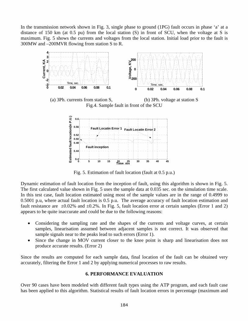
In the transmission network shown in Fig. 3, single phase to ground (1PG) fault occurs in phase ‘a’ at a distance of 150 km (at 0.5 pu) from the local station (S) in front of SCU, when the voltage at S is maximum. Fig. 5 shows the currents and voltages from the local station. Initial load prior to the fault is 300MW and –200MVR flowing from station S to R.
0 0.02 0.04 0.06 0.08 0.1-3-2
0
234
Cur
rent
, KA
Time, sec.
0 0.02 0.04 0.06 0.08 0.1
-200
0
200
Volta
ge, K
V
Time, sec.
(a) 3Ph. currents from station S, (b) 3Ph. voltage at station S Fig.4. Sample fault in front of the SCU
0 5 10 15 20 25 30 35 40 450.4
0.44
0.48
0.52
0.56
0.6
Time, msEstim
ated
faul
t loc
atio
n(in
P.U
.)
Fault Locatin Error 1 Fault Locatin Error 2
0.50
Fault inception
Fig. 5. Estimation of fault location (fault at 0.5 p.u.) Dynamic estimation of fault location from the inception of fault, using this algorithm is shown in Fig. 5. The first calculated value shown in Fig. 5 uses the sample data at 0.035 sec. on the simulation time scale. In this test case, fault location estimated using most of the sample values are in the range of 0.4999 to 0.5001 p.u, where actual fault location is 0.5 p.u. The average accuracy of fault location estimation and fault resistance are ±0.02% and ±0.2%. In Fig. 5, fault location error at certain samples (Error 1 and 2) appears to be quite inaccurate and could be due to the following reasons:
• Considering the sampling rate and the shapes of the currents and voltage curves, at certain samples, linearisation assumed between adjacent samples is not correct. It was observed that sample signals near to the peaks lead to such errors (Error 1).
• Since the change in MOV current closer to the knee point is sharp and linearisation does not produce accurate results. (Error 2)
Since the results are computed for each sample data, final location of the fault can be obtained very accurately, filtering the Error 1 and 2 by applying numerical processes to raw results.
6. PERFORMANCE EVALUATION
Over 90 cases have been modeled with different fault types using the ATP program, and each fault case has been applied to this algorithm. Statistical results of fault location errors in percentage (maximum and
184
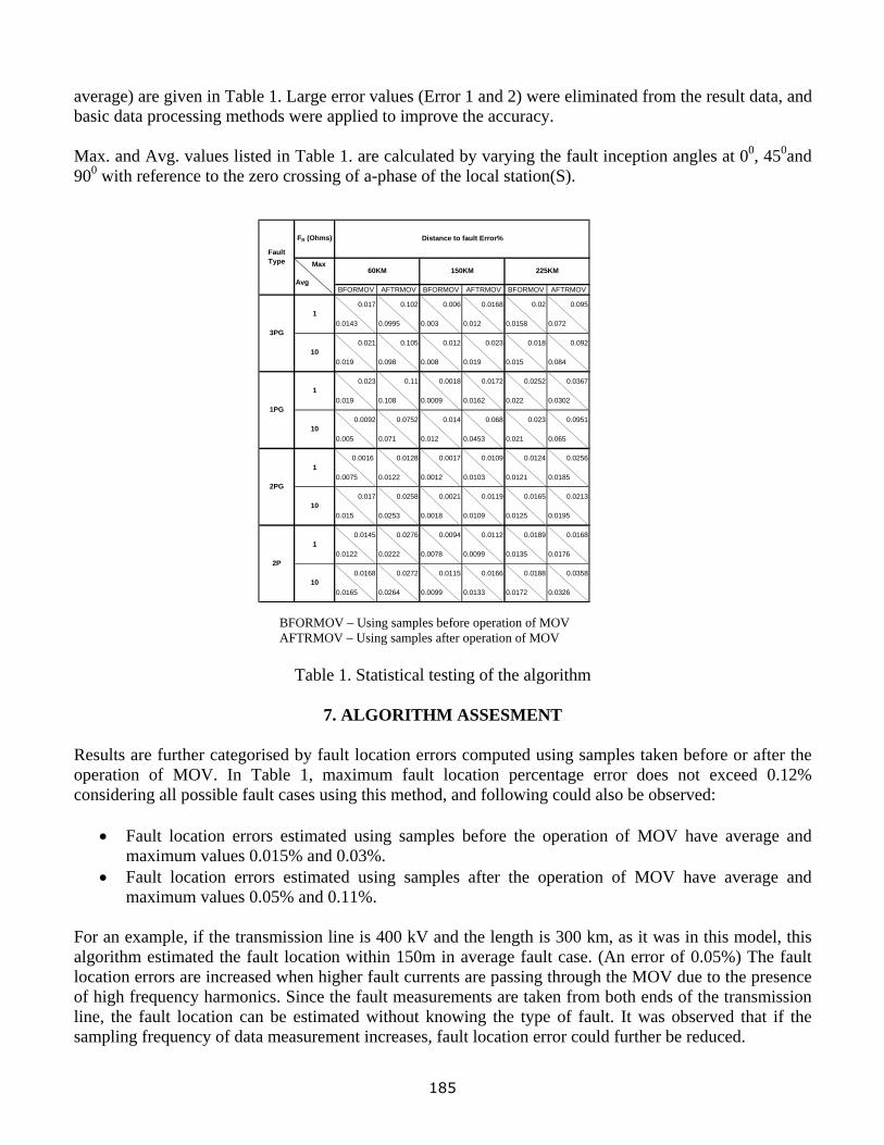
average) are given in Table 1. Large error values (Error 1 and 2) were eliminated from the result data, and basic data processing methods were applied to improve the accuracy. Max. and Avg. values listed in Table 1. are calculated by varying the fault inception angles at 00, 450and 900 with reference to the zero crossing of a-phase of the local station(S).
ce
MOV
0.00
0.01
0.00
0.01
0.00
0.00
0.00
0.01
BFORMOV AFTRMOV BFOR AFTRMOV BFORMOV AFTRMOV
0.017 0.102 6 0.0168 0.02 0.095
0.0143 0.0995 0.003 0.012 0.0158 0.072
0.021 0.105 2 0.023 0.018 0.092
0.019 0.098 0.008 0.019 0.015 0.084
0.023 0.11 18 0.0172 0.0252 0.0367
0.019 0.108 0.0009 0.0162 0.022 0.0302
0.0092 0.0752 4 0.068 0.023 0.0951
0.005 0.071 0.012 0.0453 0.021 0.065
0.0016 0.0128 17 0.0109 0.0124 0.0256
0.0075 0.0122 0.0012 0.0103 0.0121 0.0185
0.017 0.0258 21 0.0119 0.0165 0.0213
0.015 0.0253 0.0018 0.0109 0.0125 0.0195
0.0145 0.0276 94 0.0112 0.0189 0.0168
0.0122 0.0222 0.0078 0.0099 0.0135 0.0176
0.0168 0.0272 15 0.0166 0.0188 0.0358
0.0165 0.0264 0.0099 0.0133 0.0172 0.0326
1
1
10
1PG
2PG
2P
10
1
10
Distan to fault Error%FR (Ohms)
Fault Type
3PG
150KM 225KM60KM
1
10
Max
Avg
BFORMOV – Using samples before operation of MOV AFTRMOV – Using samples after operation of MOV
Table 1. Statistical testing of the algorithm
7. ALGORITHM ASSESMENT Results are further categorised by fault location errors computed using samples taken before or after the operation of MOV. In Table 1, maximum fault location percentage error does not exceed 0.12% considering all possible fault cases using this method, and following could also be observed:
• Fault location errors estimated using samples before the operation of MOV have average and maximum values 0.015% and 0.03%.
• Fault location errors estimated using samples after the operation of MOV have average and maximum values 0.05% and 0.11%.
For an example, if the transmission line is 400 kV and the length is 300 km, as it was in this model, this algorithm estimated the fault location within 150m in average fault case. (An error of 0.05%) The fault location errors are increased when higher fault currents are passing through the MOV due to the presence of high frequency harmonics. Since the fault measurements are taken from both ends of the transmission line, the fault location can be estimated without knowing the type of fault. It was observed that if the sampling frequency of data measurement increases, fault location error could further be reduced.
185
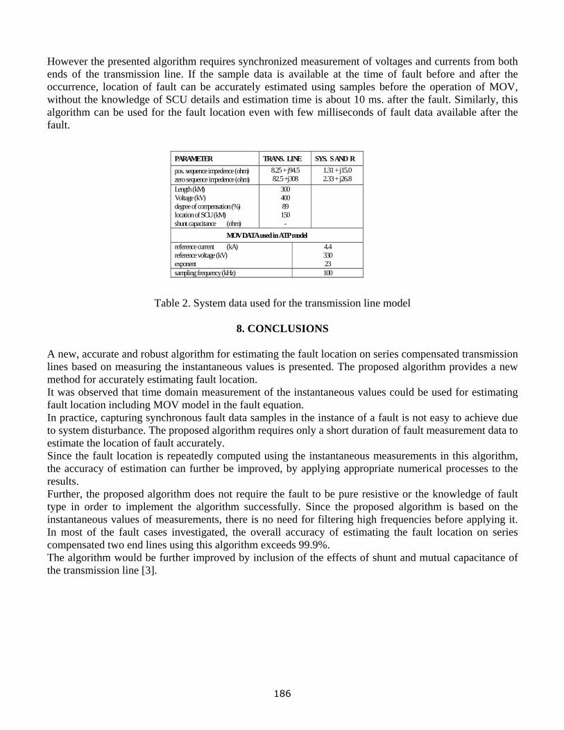
However the presented algorithm requires synchronized measurement of voltages and currents from both ends of the transmission line. If the sample data is available at the time of fault before and after the occurrence, location of fault can be accurately estimated using samples before the operation of MOV, without the knowledge of SCU details and estimation time is about 10 ms. after the fault. Similarly, this algorithm can be used for the fault location even with few milliseconds of fault data available after the fault.
PARAMETER TRANS. LINE SYS. S AND R pos. sequence impedence (ohm) zero sequence impedence (ohm)
8.25 + j94.5 82.5 +j308
1.31 + j15.0 2.33 + j26.8
Length (kM) Voltage (kV) degree of compensation (%) location of SCU (kM) shunt capacitance (ohm)
300 400 89 150 -
MOV DATA used in ATP model reference current (kA) reference voltage (kV) exponent
4.4 330 23
sampling frequency (kHz) 100
Table 2. System data used for the transmission line model
8. CONCLUSIONS
A new, accurate and robust algorithm for estimating the fault location on series compensated transmission lines based on measuring the instantaneous values is presented. The proposed algorithm provides a new method for accurately estimating fault location. It was observed that time domain measurement of the instantaneous values could be used for estimating fault location including MOV model in the fault equation. In practice, capturing synchronous fault data samples in the instance of a fault is not easy to achieve due to system disturbance. The proposed algorithm requires only a short duration of fault measurement data to estimate the location of fault accurately. Since the fault location is repeatedly computed using the instantaneous measurements in this algorithm, the accuracy of estimation can further be improved, by applying appropriate numerical processes to the results. Further, the proposed algorithm does not require the fault to be pure resistive or the knowledge of fault type in order to implement the algorithm successfully. Since the proposed algorithm is based on the instantaneous values of measurements, there is no need for filtering high frequencies before applying it. In most of the fault cases investigated, the overall accuracy of estimating the fault location on series compensated two end lines using this algorithm exceeds 99.9%. The algorithm would be further improved by inclusion of the effects of shunt and mutual capacitance of the transmission line [3].
186
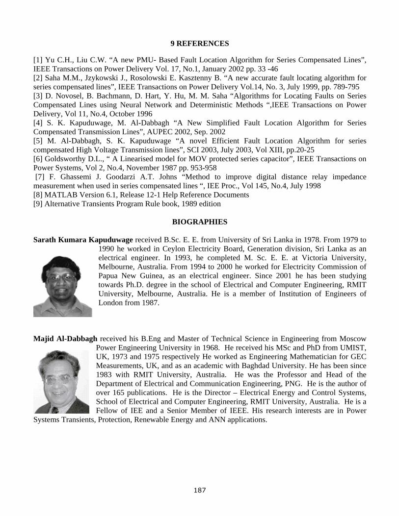
9 REFERENCES
[1] Yu C.H., Liu C.W. “A new PMU- Based Fault Location Algorithm for Series Compensated Lines”, IEEE Transactions on Power Delivery Vol. 17, No.1, January 2002 pp. 33 -46 [2] Saha M.M., Jzykowski J., Rosolowski E. Kasztenny B. “A new accurate fault locating algorithm for series compensated lines”, IEEE Transactions on Power Delivery Vol.14, No. 3, July 1999, pp. 789-795 [3] D. Novosel, B. Bachmann, D. Hart, Y. Hu, M. M. Saha “Algorithms for Locating Faults on Series Compensated Lines using Neural Network and Deterministic Methods “,IEEE Transactions on Power Delivery, Vol 11, No.4, October 1996 [4] S. K. Kapuduwage, M. Al-Dabbagh “A New Simplified Fault Location Algorithm for Series Compensated Transmission Lines”, AUPEC 2002, Sep. 2002 [5] M. Al-Dabbagh, S. K. Kapuduwage “A novel Efficient Fault Location Algorithm for series compensated High Voltage Transmission lines”, SCI 2003, July 2003, Vol XIII, pp.20-25 [6] Goldsworthy D.L., “ A Linearised model for MOV protected series capacitor”, IEEE Transactions on Power Systems, Vol 2, No.4, November 1987 pp. 953-958 [7] F. Ghassemi J. Goodarzi A.T. Johns “Method to improve digital distance relay impedance measurement when used in series compensated lines “, IEE Proc., Vol 145, No.4, July 1998 [8] MATLAB Version 6.1, Release 12-1 Help Reference Documents [9] Alternative Transients Program Rule book, 1989 edition
BIOGRAPHIES Sarath Kumara Kapuduwage received B.Sc. E. E. from University of Sri Lanka in 1978. From 1979 to
1990 he worked in Ceylon Electricity Board, Generation division, Sri Lanka as an electrical engineer. In 1993, he completed M. Sc. E. E. at Victoria University, Melbourne, Australia. From 1994 to 2000 he worked for Electricity Commission of Papua New Guinea, as an electrical engineer. Since 2001 he has been studying towards Ph.D. degree in the school of Electrical and Computer Engineering, RMIT University, Melbourne, Australia. He is a member of Institution of Engineers of London from 1987.
Majid Al-Dabbagh received his B.Eng and Master of Technical Science in Engineering from Moscow
Power Engineering University in 1968. He received his MSc and PhD from UMIST, UK, 1973 and 1975 respectively He worked as Engineering Mathematician for GEC Measurements, UK, and as an academic with Baghdad University. He has been since 1983 with RMIT University, Australia. He was the Professor and Head of the Department of Electrical and Communication Engineering, PNG. He is the author of over 165 publications. He is the Director – Electrical Energy and Control Systems, School of Electrical and Computer Engineering, RMIT University, Australia. He is a Fellow of IEE and a Senior Member of IEEE. His research interests are in Power
Systems Transients, Protection, Renewable Energy and ANN applications.
187

Using Instantaneous Values for Estimating Fault Locations on series compensated Transmission Lines
Majid Al-Dabbagh and Sarath K. Kapuduwage
Electrical Energy and Control Systems School of Electrical and Computer Engineering
RMIT University, Melbourne, Australia Abstract— Fault location estimation hitherto is based on using the filtered RMS values from both ends of the line. In this paper, a new method for locating faults on series compensated high voltage transmission lines, based on the instantaneous values is proposed. Based on the results achieved with the new algorithm, using instantaneous values, the distance to fault location is estimated very accurately [5]. However, the accuracy of the fault location is limited to the ability to capture data samples before the operation of the MOV. The proposed algorithm incorporates special techniques to avoid the limitation caused by the operation of the MOV. It is formal that although the accuracy of fault location using the algorithm proposed is slightly reduced, but still acceptable. This paper describes the new algorithm and examines its accuracy as compared to other method [5]. Keywords—fault location, series compensated lines, instantaneous values
1. INTRODUCTION The introduction of series capacitors in high voltage transmission lines brought several advantages to power system operations, such as improving power transfer capability, transient stability and damping power system oscillations. Under a fault conditions, the voltage drop across the capacitor can be dangerously high and metal oxide varistor [MOV] is used in parallel with the capacitors to protect them against such conditions. Due to the operation of MOV, which has nonlinear characteristic, fault estimation using impedance measurement techniques can no longer be used to estimate the location of a fault accurately [1, 2]. In order to estimate fault locations accurately, the voltage drop of series compensation unit is required to be computed precisely [7]. However, the existing methods available for such computations induce considerable errors in fault location estimation, due to the complexity of the series compensation units [1]. The proposed algorithm in this paper uses instantaneous measured data from the faulted power network, taking into consideration the operation of MOV, to estimate the voltage drop across the series capacitor accurately. Once the uncertain voltage drop across the capacitor is deducted from the fault equation, fault location can be estimated by calculating the voltage drop across the transmission line. The basic arrangement of series compensation of a transmission line is a series capacitor (C) in parallel with a metal oxide resistor (MOV) is shown in Fig. 1 Under fault conditions, operation of the MOV introduces additional transients in the transmission network, which will render the location of the fault difficult to estimate accurately.
188
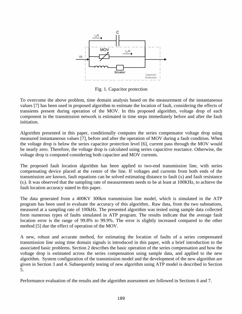
C
MOV
BreakerCapacitorProtection
If(t)
Icp(t)
Imv(t)
Fig. 1. Capacitor protection To overcome the above problem, time domain analysis based on the measurement of the instantaneous values [7] has been used in proposed algorithm to estimate the location of fault, considering the effects of transients present during operation of the MOV. In this proposed algorithm, voltage drop of each component in the transmission network is estimated in time steps immediately before and after the fault initiation. Algorithm presented in this paper, conditionally computes the series compensator voltage drop using measured instantaneous values [7], before and after the operation of MOV during a fault condition. When the voltage drop is below the series capacitor protection level [6], current pass through the MOV would be nearly zero. Therefore, the voltage drop is calculated using series capacitive reactance. Otherwise, the voltage drop is computed considering both capacitor and MOV currents. The proposed fault location algorithm has been applied to two-end transmission line, with series compensating device placed at the centre of the line. If voltages and currents from both ends of the transmission are known, fault equations can be solved estimating distance to fault (x) and fault resistance (rf). It was observed that the sampling rate of measurements needs to be at least at 100KHz, to achieve the fault location accuracy stated in this paper. The data generated from a 400KV 300km transmission line model, which is simulated in the ATP program has been used to evaluate the accuracy of this algorithm.. Raw data, from the two substations, measured at a sampling rate of 100kHz. The presented algorithm was tested using sample data collected form numerous types of faults simulated in ATP program. The results indicate that the average fault location error is the range of 99.8% to 99.9%. The error is slightly increased compared to the other method [5] due the effect of operation of the MOV. A new, robust and accurate method, for estimating the location of faults of a series compensated transmission line using time domain signals is introduced in this paper, with a brief introduction to the associated basic problems. Section 2 describes the basic operation of the series compensation and how the voltage drop is estimated across the series compensation using sample data, and applied to the new algorithm. System configuration of the transmission model and the development of the new algorithm are given in Section 3 and 4. Subsequently testing of new algorithm using ATP model is described in Section 5. Performance evaluation of the results and the algorithm assessment are followed in Sections 6 and 7.
189

2. SERIES COMPENSATOR MODEL
Fig. 1 shows the typical configuration of the series compensation device, with its basic protection mechanism. During normal operations, the series capacitor (C) generates leading VARS to compensate some of the VAR consumed by the network. The Metal Oxide Varistor (MOV) is the main protection device, which operates when an over voltage is detected across the capacitor. With a short circuit on the line, the capacitor is subjected to an extremely high voltage, which is controlled by the conduction of MOV. The voltage protection level of MOV (1.5pu to 2.0pu) is determined with reference to the capacitor voltage drop with rated current flowing through it [6]. The VI–characteristics of the MOV can be approximated by a nonlinear equation:
⎟⎠⎞
⎜⎝⎛=
VREFVpi
q
* (1) Where p and VREF are the reference quantities of the MOV and typically q is in the order of 20 to 30 [9]. The Circuit Breaker provides the protection of MOV to limit the absorption energy during operation. As shown in Fig. 1, if the fault current passing through the series compensation unit (SCU) is If, under any operational condition it can be shown that:
If (t) = Icp(t) + Imv(t) (2) where Icp and Imv are the capacitor and MOV currents. Under normal load conditions, line current Il = Icp and Imv = 0. Under fault conditions, MOV begins to conduct when fault current exceeds 0.98Ipu, where Ipu is defined with reference to the capacitor currents. ( Ipu = Icp / Ipr) where Ipr is the capacitor protective level current. Therefore, faulted SCU voltage drop need to be estimated in two ways: A. MOV is not conducting If the fault current is known, the voltage drop across the capacitor can be expressed in terms of instantaneous values:
dttC
Ttt tTt Fcpcp iVV )(1)()( ∫ −+−= (3)
Where Vcp(t) is the current voltage drop, and T is the sampling time of the measured fault current. By applying the Trapezoidal Rule, the integral part in equation (3) can be expressed in terms of the sampled currents as follows:
[ ])()(2
)()( TttCTTtt IIVV ffcpcp −++−= (4)
B. MOV is conducting Assume that MOV characteristics at a given time t can be linearised around the previous time sample ( t –T ), MOV current can be deduced from: [ ])()()()( Tttgtt VVII mvmvmvmv −−+= (5)
190
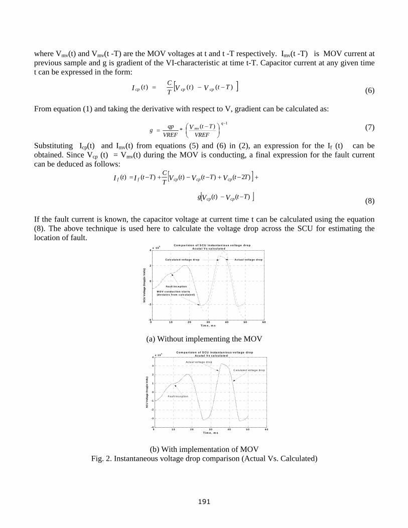
where Vmv(t) and Vmv(t -T) are the MOV voltages at t and t -T respectively. Imv(t -T) is MOV current at previous sample and g is gradient of the VI-characteristic at time t-T. Capacitor current at any given time t can be expressed in the form: [ ])()()( Ttt
TCt VVI cpcpcp −−= (6)
From equation (1) and taking the derivative with respect to V, gradient can be calculated as:
(7) ⎟⎠⎞
⎜⎝⎛ −
=−
VREFTt
VREFqpg V mv
q)(*1
Substituting Icp(t) and Imv(t) from equations (5) and (6) in (2), an expression for the If (t) can be obtained. Since Vcp (t) = Vmv(t) during the MOV is conducting, a final expression for the fault current can be deduced as follows: [ ] +−+−−+−= )2()()()()( TtTtt
TCTtt VVVII cpcpcpff
[ ])()( Tttg VV cpcp −− (8)
If the fault current is known, the capacitor voltage at current time t can be calculated using the equation (8). The above technique is used here to calculate the voltage drop across the SCU for estimating the location of fault.
0 10 20 30 40 50 60-5
-3
0
2
4x 10 5
T im e , m s
SC
U V
olta
ge D
rop(
in V
olts
)
C o m p a risio n o f S CU in sta n ta n io u s vo l ta g e d ro p A cu ta l V s ca lcu la te d
Fa ult Inc e ption
M O V c onduc tion s ta r ts (de via te s from c a lc u la te d)
Ac tua l vo lta ge drop Ca lc u la te d vo lta ge drop
(a) Without implementing the MOV
0 1 0 2 0 3 0 4 0 5 0 6 0-4
-3
-2
-1
0
1
2
3
4x 1 0 5
T im e , m s
SCU
Vol
tage
Dro
p(in
Vol
ts)
C o m p a risio n o f S CU in sta n ta n io u s vo l ta g e d ro p A cu ta l V s ca lcu la te d
Fa u lt In ce p tio n
Ac tu a l vo l ta g e d ro p
C a lu la te d vo lta g e d ro p
(b) With implementation of MOV
Fig. 2. Instantaneous voltage drop comparison (Actual Vs. Calculated)
191
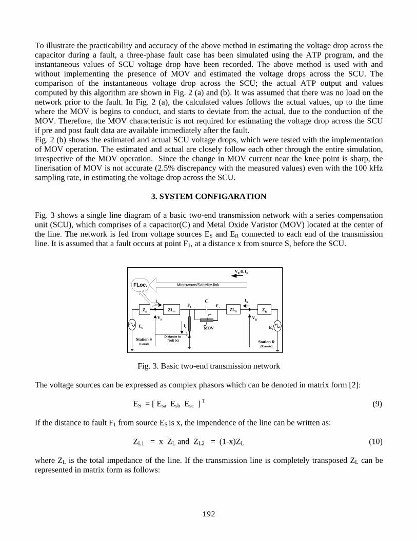
To illustrate the practicability and accuracy of the above method in estimating the voltage drop across the capacitor during a fault, a three-phase fault case has been simulated using the ATP program, and the instantaneous values of SCU voltage drop have been recorded. The above method is used with and without implementing the presence of MOV and estimated the voltage drops across the SCU. The comparison of the instantaneous voltage drop across the SCU; the actual ATP output and values computed by this algorithm are shown in Fig. 2 (a) and (b). It was assumed that there was no load on the network prior to the fault. In Fig. 2 (a), the calculated values follows the actual values, up to the time where the MOV is begins to conduct, and starts to deviate from the actual, due to the conduction of the MOV. Therefore, the MOV characteristic is not required for estimating the voltage drop across the SCU if pre and post fault data are available immediately after the fault. Fig. 2 (b) shows the estimated and actual SCU voltage drops, which were tested with the implementation of MOV operation. The estimated and actual are closely follow each other through the entire simulation, irrespective of the MOV operation. Since the change in MOV current near the knee point is sharp, the linerisation of MOV is not accurate (2.5% discrepancy with the measured values) even with the 100 kHz sampling rate, in estimating the voltage drop across the SCU.
3. SYSTEM CONFIGARATION Fig. 3 shows a single line diagram of a basic two-end transmission network with a series compensation unit (SCU), which comprises of a capacitor(C) and Metal Oxide Varistor (MOV) located at the center of the line. The network is fed from voltage sources ES and ER connected to each end of the transmission line. It is assumed that a fault occurs at point F1, at a distance x from source S, before the SCU. VR & IR
FLoc.
ES
Station S(Local)
ZS ZL11 ZL22 ZR
MOV
C
ER
F2
ISIR
IF
VS VR
Station R(Remote)
Microwave/Sattelite link
F1
Distance to fault (x)
Fig. 3. Basic two-end transmission network The voltage sources can be expressed as complex phasors which can be denoted in matrix form [2]:
ES = [ Esa Esb Esc ] T (9) If the distance to fault F1 from source ES is x, the impendence of the line can be written as:
ZL1 = x ZL and ZL2 = (1-x)ZL (10) where ZL is the total impedance of the line. If the transmission line is completely transposed ZL can be represented in matrix form as follows:
192

[ ]⎥⎥⎥
⎦
⎤
⎢⎢⎢
⎣
⎡=
ZZZZZZZZZ
Z
LssLmmLmm
LmmLssLmm
LmmLmmLss
L
(11)
Where ZLss and ZLmm are self and mutual impedances of the line.
4. DEVELOPMENT OF THE NEW ALGORITHM A. Fault Location Let us consider the configuration of a two terminal transmission line as shown in Fig. 3. Assume the fault occurs on the line at F1, x kilometres from the local bus, prior to SCU. If the voltage and current at the local bus and remote buses are Vs, Is, VR and IR respectively, then the network equation of the faulted system can be written in matrix form:
(12) [ ] [ ][ ] [ ] [ ][ ] [ ]VIZxVIZxV DRLRSLs −−−=− )1( where [VD] is the voltage drop across the series compensation unit. Using IB data samples in equation (8), the instantaneous values of VD can be calculated. However, the computation of current value of VD requires its previous value. Initial values for VD can be estimated applying pre fault values to the network equations. At any given time, the instantaneous voltage drop across the impedance with inductance L and resistance R can be written in discrete form as:
[ ])()()(.)( TtItITLtIRtV −−+= (13)
Where I (t) is the current passing through the impedance at time t. Knowing IS and IR, the instantaneous values of [ZL]IS] and [ZL]IR] are calculated using equation (13). Solution for distance to fault x can be estimated for each instantaneous value using the following expression:
(14) where t0 is the time at which sample values are computed.
)()()()()()(
)(00
00000
tVZtVZtVZtVtVtV
txRS
RDBA
+++−
=
Measured voltages and computed voltage drops are 3x1 matrices for a 3-phase line and must be solved using matrix operations. B. Locating Fault with respect to SCU If the fault occurs at F2 as shown in Fig. 3, prior to the SCU, equation (12) needs to be adjusted as follows:
)()()()()()(
)(00
00000
tVZtVZtVZtVtVtV
txRR
RDBA
++−−
= (15) C. Selection Method The selection algorithm used for applying correct equations for locating faults with respect to the position of SCU can be described as follows:
193
Since the SCU is located at the middle of line, distance to the fault x could be estimated using equation (14), and the result should be in the range of x > 0 and x <= 0.5. If the value of x is not in this range, equation (15) will correctly estimate the fault location. D. Fault Resistance A general 3-phase fault model is implemented in fault location algorithm to estimate the fault resistance [1]. 3-phase fault conduction matrix can be stated in matrix form: where Rf is the aggregated fault resistance and VF is the voltage at the fault. [ ] [ ][
[ ] [ ] [ ]III
VKR
I
RSF
FFf
F
+=
=1 ] (16)
where the fault matrix KF need to be computed in relation to the type of fault [2]. Applying fault equation to the opposite side of series compensation unit: [ ] [ ] [ ][ ]IVV RRF ZLx )1( −−= (17) where VF is the voltage at the fault location. If the fault type and distance to fault are known, fault resistance can be calculated using equation (16) and (17).
5. TESTING AND EVALUATION
A. Transmission line Model In order to statistically test the accuracy and robustness of the newly developed algorithm, a two terminal, 3-phase transmission model as shown in Fig. 3, was modeled using the ATP program. The transmission line model used is 300km long and rated at 400KV. The series compensation unit is placed and fixed in the middle of the line. The supply systems are represented by mutually coupled R L branches together with ideal voltage sources [9]. The transmission line is represented by two sections of 3 -phase mutually coupled R L branches specifying positive and zero sequence impedance for each branch. The Series compensation unit consists of a capacitor and MOV and it has the v-i characteristics of ZnO surge arrester represented by a non-linear equation similar to equation (1). The flash over voltage of the gap is specified in order to fire the gap during heavy fault currents. Voltages and currents from both ends are recorded at sampling rate of 100KHz before and after fault occurrence. Total simulation time is 0.1 sec. and the fault is initiated at 0.035 sec. For statistical evaluations, the same data file was modeled using the ATP program, with minor modifications to cover the broad spectrum of faults. The system data used for this model are shown in table 2. B. Implementation of Fault Location Algorithm The new algorithm was implemented using MATLAB 6.5 software script language [8]. Row data generated from the ATP model was converted to EXCEL worksheet in order to be opened directly from MATLAB. After opening the file from MATLAB, data was further separated to individual arrays, to apply to the new algorithm. The proposed algorithm was developed using MATLAB script language.
194

In the transmission network shown in Fig. 3, single phase to ground (1PG) fault occurs in phase ‘a’ at a distance of 150 km (at 0.5 pu) from the local station (S) in front of SCU, when the voltage at S is maximum. Fig. 5 shows the currents and voltages from the local station. Initial load prior to the fault is 300MW and –200MVR flowing from station S to R.
0 0.02 0.04 0.06 0.08 0.1-3-2
0
234
Cur
rent
, KA
Time, sec.
0 0.02 0.04 0.06 0.08 0.1
-200
0
200
Volta
ge, K
V
Time, sec.
(a) 3Ph. currents from station S, (b) 3Ph. voltage at station S Fig.4. Sample fault in front of the SCU
0 5 10 15 20 25 30 35 40 450.4
0.44
0.48
0.52
0.56
0.6
Time, msEstim
ated
faul
t loc
atio
n(in
P.U
.)
Fault Locatin Error 1 Fault Locatin Error 2
0.50
Fault inception
Fig. 5. Estimation of fault location (fault at 0.5 p.u.) Dynamic estimation of fault location from the inception of fault, using this algorithm is shown in Fig. 5. The first calculated value shown in Fig. 5 uses the sample data at 0.035 sec. on the simulation time scale. In this test case, fault location estimated using most of the sample values are in the range of 0.4999 to 0.5001 p.u, where actual fault location is 0.5 p.u. The average accuracy of fault location estimation and fault resistance are ±0.02% and ±0.2%. In Fig. 5, fault location error at certain samples (Error 1 and 2) appears to be quite inaccurate and could be due to the following reasons:
• Considering the sampling rate and the shapes of the currents and voltage curves, at certain samples, linearisation assumed between adjacent samples is not correct. It was observed that sample signals near to the peaks lead to such errors (Error 1).
• Since the change in MOV current closer to the knee point is sharp and linearisation does not produce accurate results. (Error 2)
Since the results are computed for each sample data, final location of the fault can be obtained very accurately, filtering the Error 1 and 2 by applying numerical processes to raw results.
6. PERFORMANCE EVALUATION
Over 90 cases have been modeled with different fault types using the ATP program, and each fault case has been applied to this algorithm. Statistical results of fault location errors in percentage (maximum and
195

average) are given in Table 1. Large error values (Error 1 and 2) were eliminated from the result data, and basic data processing methods were applied to improve the accuracy. Max. and Avg. values listed in Table 1. are calculated by varying the fault inception angles at 00, 450and 900 with reference to the zero crossing of a-phase of the local station(S).
ce
MOV
0.00
0.01
0.00
0.01
0.00
0.00
0.00
0.01
BFORMOV AFTRMOV BFOR AFTRMOV BFORMOV AFTRMOV
0.017 0.102 6 0.0168 0.02 0.095
0.0143 0.0995 0.003 0.012 0.0158 0.072
0.021 0.105 2 0.023 0.018 0.092
0.019 0.098 0.008 0.019 0.015 0.084
0.023 0.11 18 0.0172 0.0252 0.0367
0.019 0.108 0.0009 0.0162 0.022 0.0302
0.0092 0.0752 4 0.068 0.023 0.0951
0.005 0.071 0.012 0.0453 0.021 0.065
0.0016 0.0128 17 0.0109 0.0124 0.0256
0.0075 0.0122 0.0012 0.0103 0.0121 0.0185
0.017 0.0258 21 0.0119 0.0165 0.0213
0.015 0.0253 0.0018 0.0109 0.0125 0.0195
0.0145 0.0276 94 0.0112 0.0189 0.0168
0.0122 0.0222 0.0078 0.0099 0.0135 0.0176
0.0168 0.0272 15 0.0166 0.0188 0.0358
0.0165 0.0264 0.0099 0.0133 0.0172 0.0326
1
1
10
1PG
2PG
2P
10
1
10
Distan to fault Error%FR (Ohms)
Fault Type
3PG
150KM 225KM60KM
1
10
Max
Avg
BFORMOV – Using samples before operation of MOV AFTRMOV – Using samples after operation of MOV
Table 1. Statistical testing of the algorithm
7. ALGORITHM ASSESMENT Results are further categorised by fault location errors computed using samples taken before or after the operation of MOV. In Table 1, maximum fault location percentage error does not exceed 0.12% considering all possible fault cases using this method, and following could also be observed:
• Fault location errors estimated using samples before the operation of MOV have average and maximum values 0.015% and 0.03%.
• Fault location errors estimated using samples after the operation of MOV have average and maximum values 0.05% and 0.11%.
For an example, if the transmission line is 400 kV and the length is 300 km, as it was in this model, this algorithm estimated the fault location within 150m in average fault case. (An error of 0.05%) The fault location errors are increased when higher fault currents are passing through the MOV due to the presence of high frequency harmonics. Since the fault measurements are taken from both ends of the transmission line, the fault location can be estimated without knowing the type of fault. It was observed that if the sampling frequency of data measurement increases, fault location error could further be reduced.
196

However the presented algorithm requires synchronized measurement of voltages and currents from both ends of the transmission line. If the sample data is available at the time of fault before and after the occurrence, location of fault can be accurately estimated using samples before the operation of MOV, without the knowledge of SCU details and estimation time is about 10 ms. after the fault. Similarly, this algorithm can be used for the fault location even with few milliseconds of fault data available after the fault.
PARAMETER TRANS. LINE SYS. S AND R pos. sequence impedence (ohm) zero sequence impedence (ohm)
8.25 + j94.5 82.5 +j308
1.31 + j15.0 2.33 + j26.8
Length (kM) Voltage (kV) degree of compensation (%) location of SCU (kM) shunt capacitance (ohm)
300 400 89 150 -
MOV DATA used in ATP model reference current (kA) reference voltage (kV) exponent
4.4 330 23
sampling frequency (kHz) 100
Table 2. System data used for the transmission line model
8. CONCLUSIONS
A new, accurate and robust algorithm for estimating the fault location on series compensated transmission lines based on measuring the instantaneous values is presented. The proposed algorithm provides a new method for accurately estimating fault location. It was observed that time domain measurement of the instantaneous values could be used for estimating fault location including MOV model in the fault equation. In practice, capturing synchronous fault data samples in the instance of a fault is not easy to achieve due to system disturbance. The proposed algorithm requires only a short duration of fault measurement data to estimate the location of fault accurately. Since the fault location is repeatedly computed using the instantaneous measurements in this algorithm, the accuracy of estimation can further be improved, by applying appropriate numerical processes to the results. Further, the proposed algorithm does not require the fault to be pure resistive or the knowledge of fault type in order to implement the algorithm successfully. Since the proposed algorithm is based on the instantaneous values of measurements, there is no need for filtering high frequencies before applying it. In most of the fault cases investigated, the overall accuracy of estimating the fault location on series compensated two end lines using this algorithm exceeds 99.9%. The algorithm would be further improved by inclusion of the effects of shunt and mutual capacitance of the transmission line [3].
197

9 REFERENCES
[1] Yu C.H., Liu C.W. “A new PMU- Based Fault Location Algorithm for Series Compensated Lines”, IEEE Transactions on Power Delivery Vol. 17, No.1, January 2002 pp. 33 -46 [2] Saha M.M., Jzykowski J., Rosolowski E. Kasztenny B. “A new accurate fault locating algorithm for series compensated lines”, IEEE Transactions on Power Delivery Vol.14, No. 3, July 1999, pp. 789-795 [3] D. Novosel, B. Bachmann, D. Hart, Y. Hu, M. M. Saha “Algorithms for Locating Faults on Series Compensated Lines using Neural Network and Deterministic Methods “,IEEE Transactions on Power Delivery, Vol 11, No.4, October 1996 [4] S. K. Kapuduwage, M. Al-Dabbagh “A New Simplified Fault Location Algorithm for Series Compensated Transmission Lines”, AUPEC 2002, Sep. 2002 [5] M. Al-Dabbagh, S. K. Kapuduwage “A novel Efficient Fault Location Algorithm for series compensated High Voltage Transmission lines”, SCI 2003, July 2003, Vol XIII, pp.20-25 [6] Goldsworthy D.L., “ A Linearised model for MOV protected series capacitor”, IEEE Transactions on Power Systems, Vol 2, No.4, November 1987 pp. 953-958 [7] F. Ghassemi J. Goodarzi A.T. Johns “Method to improve digital distance relay impedance measurement when used in series compensated lines “, IEE Proc., Vol 145, No.4, July 1998 [8] MATLAB Version 6.1, Release 12-1 Help Reference Documents [9] Alternative Transients Program Rule book, 1989 edition
BIOGRAPHIES Sarath Kumara Kapuduwage received B.Sc. E. E. from University of Sri Lanka in 1978. From 1979 to
1990 he worked in Ceylon Electricity Board, Generation division, Sri Lanka as an electrical engineer. In 1993, he completed M. Sc. E. E. at Victoria University, Melbourne, Australia. From 1994 to 2000 he worked for Electricity Commission of Papua New Guinea, as an electrical engineer. Since 2001 he has been studying towards Ph.D. degree in the school of Electrical and Computer Engineering, RMIT University, Melbourne, Australia. He is a member of Institution of Engineers of London from 1987.
Majid Al-Dabbagh received his B.Eng and Master of Technical Science in Engineering from Moscow
Power Engineering University in 1968. He received his MSc and PhD from UMIST, UK, 1973 and 1975 respectively He worked as Engineering Mathematician for GEC Measurements, UK, and as an academic with Baghdad University. He has been since 1983 with RMIT University, Australia. He was the Professor and Head of the Department of Electrical and Communication Engineering, PNG. He is the author of over 165 publications. He is the Director – Electrical Energy and Control Systems, School of Electrical and Computer Engineering, RMIT University, Australia. He is a Fellow of IEE and a Senior Member of IEEE. His research interests are in Power
Systems Transients, Protection, Renewable Energy and ANN applications.
198
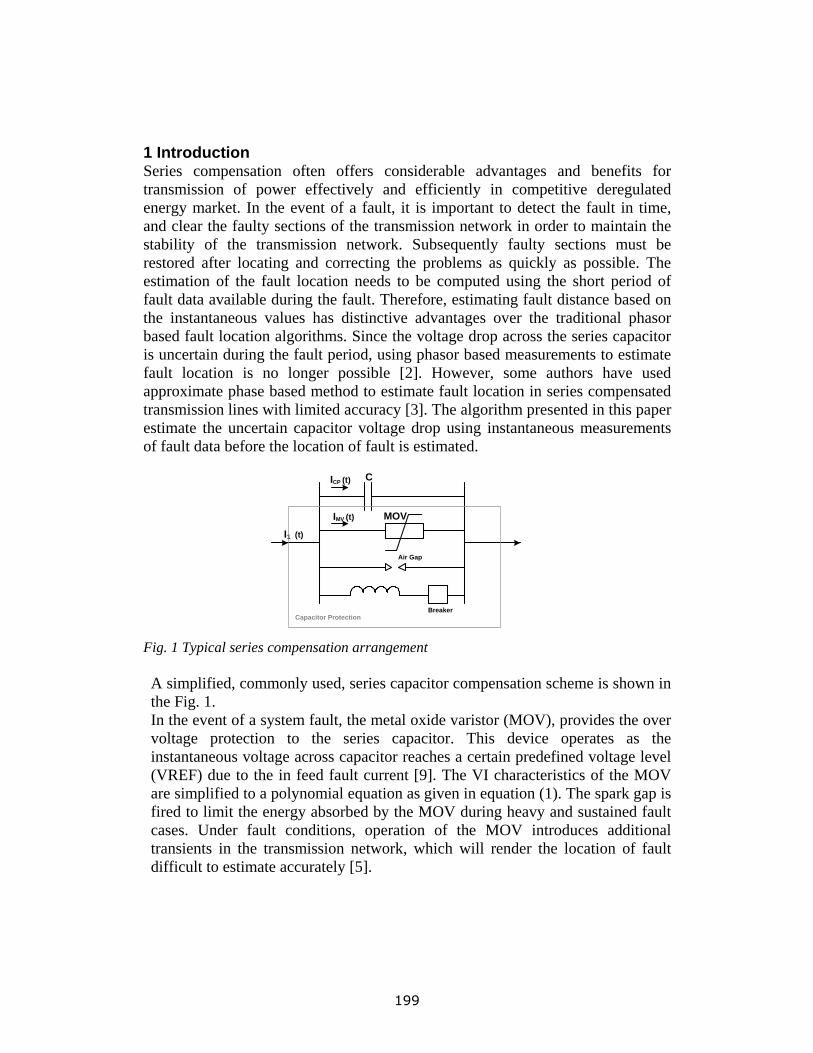
1 Introduction Series compensation often offers considerable advantages and benefits for transmission of power effectively and efficiently in competitive deregulated energy market. In the event of a fault, it is important to detect the fault in time, and clear the faulty sections of the transmission network in order to maintain the stability of the transmission network. Subsequently faulty sections must be restored after locating and correcting the problems as quickly as possible. The estimation of the fault location needs to be computed using the short period of fault data available during the fault. Therefore, estimating fault distance based on the instantaneous values has distinctive advantages over the traditional phasor based fault location algorithms. Since the voltage drop across the series capacitor is uncertain during the fault period, using phasor based measurements to estimate fault location is no longer possible [2]. However, some authors have used approximate phase based method to estimate fault location in series compensated transmission lines with limited accuracy [3]. The algorithm presented in this paper estimate the uncertain capacitor voltage drop using instantaneous measurements of fault data before the location of fault is estimated. C
MOV
Air Gap
Breaker
ICP (t)
IMV (t)
I1 (t)
Capacitor Protection
Fig. 1 Typical series compensation arrangement A simplified, commonly used, series capacitor compensation scheme is shown in the Fig. 1. In the event of a system fault, the metal oxide varistor (MOV), provides the over voltage protection to the series capacitor. This device operates as the instantaneous voltage across capacitor reaches a certain predefined voltage level (VREF) due to the in feed fault current [9]. The VI characteristics of the MOV are simplified to a polynomial equation as given in equation (1). The spark gap is fired to limit the energy absorbed by the MOV during heavy and sustained fault cases. Under fault conditions, operation of the MOV introduces additional transients in the transmission network, which will render the location of fault difficult to estimate accurately [5].
199
Since the proposed algorithm is based on the measurements of instantaneous values, the transient presence during the operation of the MOV will have fewer effects in estimation of the fault location. The algorithm presented in this paper is developed for a two-end transmission line with series compensation is located at the centre of the line. This algorithm uses instantaneous measurements of synchronised fault data from both ends of the line for very short duration to estimate fault location accurately. In the case of long transmission line, the synchronised fault data measurements can be accurately recorded with absolute time references, using Global Positioning System (GPS). Application of high performance GPS recorders is not expensive and easily available nowadays, and can be used to record signals up to the accuracy of 100ns at 95% probability [12]. Fault measurement samples from both ends can be synchronised, with very high accuracy using more intelligent type of master clock [12]. If instantaneous values of voltages and currents from both ends of the transmission line are known, fault equation can be solved estimating distance to fault (x) and fault resistance (rf) for each time step. It was observed that the sampling rate of measurements needs minimum of 100 kHz to achieve the fault location accuracy stated in this paper. A 400KV, 300km two ends transmission line was modelled and simulated using ATP software and instantaneous fault signals were recorded to evaluate the accuracy of this algorithm. The sampling rate of the measurements was set at 100 KHz. The algorithm for the estimation of fault location and resistance was developed using MATLAB script language. Simulation of numerous types of fault cases have been conducted with many variations and the recorded data has been input in algorithm to compute the fault location and resistance for each time step. The result arrays have been further processed numerically to obtain the average values of the fault distance and resistance. The results indicate that the average fault location error estimated using this algorithm is below 0.2%. A new, robust and accurate method, for estimating the location of faults of a series compensated transmission line using time domain signals is introduced in this paper, with a brief introduction to the associated basic problems. Section 2 describes the basic operation of the series compensation and how the voltage drop is estimated across the series compensation using sample data, and applied to the new algorithm. System configuration of the transmission model and the development of the new algorithm are given in Section 3 and 4. Subsequently testing of new algorithm using ATP model is described in Section 5. Finally the evaluation of the results and conclusions are followed in Sections 6 and 7.
200
2. Series Compensation Model Fig. 1 shows the typical configuration of the series compensation device, and its basic protection mechanism. The complicity of developing an accurate method of computing the location fault is heavily dependent on the protection devices incorporated in series compensation. The MOV conducts immediately after the capacitor instantaneous voltage drop across the capacitor exceeds a certain voltage level (VREF). The VI characteristics of the MOV can be expressed by a nonlinear equation:
⎟⎟⎠
⎞⎜⎜⎝
⎛=
VREFp V
ICP
q
MOV * (1) Where p and VREF are the reference quantities of the MOV and typically, q is in the order of 20 to 30 [13]. During heavy and sustaining fault currents, the MOV exceeds its maximum energy absorption limit. The spark gap is fired to protect this device of being over burdened as shown in Fig. 1. The operating level of the spark gap is derived from the quantity and duration of the fault current continues to pass through the MOV. If the fault current is I f under any operational conditions, other than the spark gap is in operation, it can be expressed in terms of:
(2) )()()( tI mvtI cptI f += where I CP and I MV are capacitor current and MOV current which flow through the series compensation circuit at a given time t. Under normal load conditions, line current Il = I cp and I mv = 0. Under fault conditions, over voltage protection operates, when fault current exceeds 0.98Ipu, where I pu is defined with reference to the capacitor currents. (I pu = I cp / I pr) I pr is the capacitor protective level current [2]. Therefore, faulted SCU voltage drop needs to be estimated considering these conditions. 2.1 MOV is not conducting If the fault current is known, the voltage drop across the capacitor can be expressed by instantaneous values:
dttC
Ttt tTt Fcpcp iVV )(1)()( ∫ −+−= (3)
Where V cp (t) is the current voltage drop and T is the sampling time of the measured fault current. By applying the trapezoidal rule, the integral part in equation (3) can be expressed in terms of the sampled currents as follows:
(4)
[ ])()(2
)()( TttCTTtt IIVV ffcpcp −++−=
201
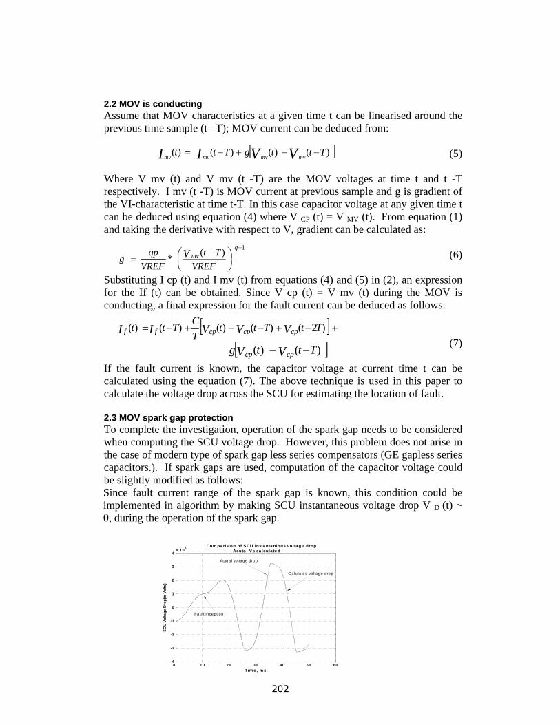
2.2 MOV is conducting Assume that MOV characteristics at a given time t can be linearised around the previous time sample (t –T); MOV current can be deduced from:
[ ])()()()( TttgTtt VVII mvmvmvmv −−+−= (5) Where V mv (t) and V mv (t -T) are the MOV voltages at time t and t -T respectively. I mv (t -T) is MOV current at previous sample and g is gradient of the VI-characteristic at time t-T. In this case capacitor voltage at any given time t can be deduced using equation (4) where V CP (t) = V MV (t). From equation (1) and taking the derivative with respect to V, gradient can be calculated as:
⎟⎠⎞
⎜⎝⎛ −
=−
VREFTt
VREFqpg V mv
q)(*1
(6) Substituting I cp (t) and I mv (t) from equations (4) and (5) in (2), an expression for the If (t) can be obtained. Since V cp (t) = V mv (t) during the MOV is conducting, a final expression for the fault current can be deduced as follows:
0 10 20 30 40 50 60-4
-3
-2
-1
0
1
2
3
4x 10 5
Tim e , m s
SCU
Vol
tage
Dro
p(in
Vol
ts)
Com pa rision of S CU insta nta nious volta ge drop Acuta l V s ca lcula te d
Fau lt Incep tion
Actua l vo ltage d rop
C alu la ted vo ltage drop
(7)
[ ] +−+−−+−= )2()()()()( TtTttTCTtt VVVII cpcpcpff
[ ])()( Tttg VV cpcp −− If the fault current is known, the capacitor voltage at current time t can be calculated using the equation (7). The above technique is used in this paper to calculate the voltage drop across the SCU for estimating the location of fault. 2.3 MOV spark gap protection To complete the investigation, operation of the spark gap needs to be considered when computing the SCU voltage drop. However, this problem does not arise in the case of modern type of spark gap less series compensators (GE gapless series capacitors.). If spark gaps are used, computation of the capacitor voltage could be slightly modified as follows: Since fault current range of the spark gap is known, this condition could be implemented in algorithm by making SCU instantaneous voltage drop V D (t) ~ 0, during the operation of the spark gap.
202
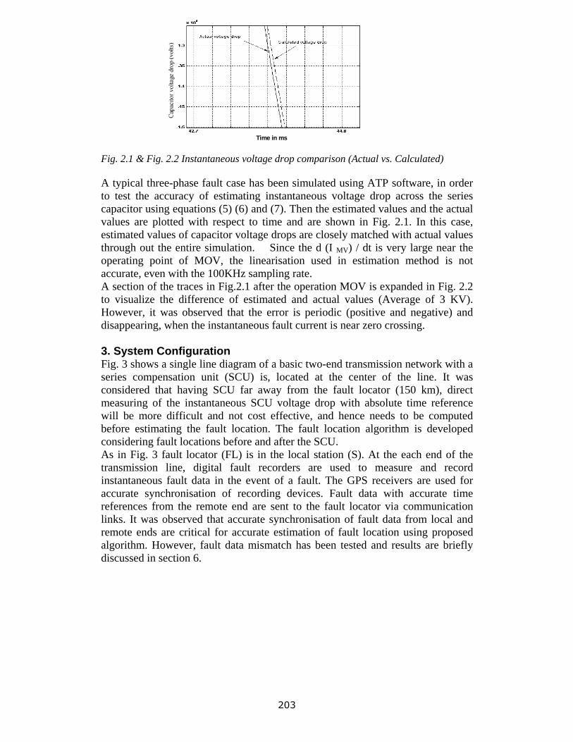
Time in ms
Fig. 2.1 & Fig. 2.2 Instantaneous voltage drop comparison (Actual vs. Calculated) A typical three-phase fault case has been simulated using ATP software, in order to test the accuracy of estimating instantaneous voltage drop across the series capacitor using equations (5) (6) and (7). Then the estimated values and the actual values are plotted with respect to time and are shown in Fig. 2.1. In this case, estimated values of capacitor voltage drops are closely matched with actual values through out the entire simulation. Since the d (I MV) / dt is very large near the operating point of MOV, the linearisation used in estimation method is not accurate, even with the 100KHz sampling rate. A section of the traces in Fig.2.1 after the operation MOV is expanded in Fig. 2.2 to visualize the difference of estimated and actual values (Average of 3 KV). However, it was observed that the error is periodic (positive and negative) and disappearing, when the instantaneous fault current is near zero crossing. 3. System Configuration Fig. 3 shows a single line diagram of a basic two-end transmission network with a series compensation unit (SCU) is, located at the center of the line. It was considered that having SCU far away from the fault locator (150 km), direct measuring of the instantaneous SCU voltage drop with absolute time reference will be more difficult and not cost effective, and hence needs to be computed before estimating the fault location. The fault location algorithm is developed considering fault locations before and after the SCU. As in Fig. 3 fault locator (FL) is in the local station (S). At the each end of the transmission line, digital fault recorders are used to measure and record instantaneous fault data in the event of a fault. The GPS receivers are used for accurate synchronisation of recording devices. Fault data with accurate time references from the remote end are sent to the fault locator via communication links. It was observed that accurate synchronisation of fault data from local and remote ends are critical for accurate estimation of fault location using proposed algorithm. However, fault data mismatch has been tested and results are briefly discussed in section 6.
203
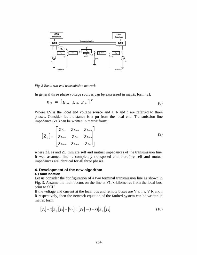
(1-x)ZL
MOV
C
VF
F2
IF
F1
Station R
ES
Station S
ZS xZL
IS
VS
FLZR
ER
IR
VR
GPSReceiver
DFR
GPSReceiver
DFRCoomunication lines
Fig. 3 Basic two-end transmission network In general three phase voltage sources can be expressed in matrix form [2]; [ ]EEEE scsbsa
TS = (8)
Where ES is the local end voltage source and a, b and c are referred to three phases. Consider fault distance is x pu from the local end. Transmission line impedance (ZL) can be written in matrix form:
[ ]⎥⎥⎥
⎦
⎤
⎢⎢⎢
⎣
⎡=
ZZZ
ZZZ
ZZZ
LssLmmLmm
LmmLssLmm
LmmLmmLss
LZ
(9) where ZL ss and ZL mm are self and mutual impedances of the transmission line. It was assumed line is completely transposed and therefore self and mutual impedances are identical for all three phases. 4. Development of the new algorithm 4.1 fault location Let us consider the configuration of a two terminal transmission line as shown in Fig. 3. Assume the fault occurs on the line at F1, x kilometres from the local bus, prior to SCU. If the voltage and current at the local bus and remote buses are V s, I s, V R and I R respectively, then the network equation of the faulted system can be written in matrix form:
[ ] [ ][ ] [ ] [ ] [ ][ ]IVVIV RLRDSLs ZxZx )1( −−=−− (10)
204
where [VD] is the voltage drop across the series compensation unit. If the fault occurs on the line at F2, after SCU, the fault equation could be modified as follows:
[ ] [ ][ ] [ ] [ ][ ] [ ]VIZxVIZxV DRLRSLs −−−=− )1( (11) In both cases, capacitor instantaneous voltage drops can be computed either using IR or IS. [ZL][IS] instantaneous voltage drops can be computed using differential equation in the time domain and takes the form:
⎥⎥⎥
⎦
⎤
⎢⎢⎢
⎣
⎡
⎥⎥⎥
⎦
⎤
⎢⎢⎢
⎣
⎡+⎥⎥⎥
⎦
⎤
⎢⎢⎢
⎣
⎡
⎥⎥⎥
⎦
⎤
⎢⎢⎢
⎣
⎡
dtdtdt
dI
dI
dI
XMM
MXM
MMX
R
I
I
R
R
R
Sc
Sb
Sa
LcLcbLca
LbcLbLba
LacLabLa
Sc
Sb
Sa
Lc
Lb
La
///
(12)
where RL and XL are the line total resistance and self inductance. ML is the mutual inductance between phases. [ZL][IR] also can be computed similarly and both are of 3 x 1 matrices. Knowing capacitor voltage drop [VD], equation (10) and (11) can be solved to compute the fault location x for each time sampling step. 4.2 selection method Since the location of the fault is not known prior to the estimation of fault distance, results obtained from both equations are not valid. To solve this problem, first compute the fault location using equation (10) and (11). Finding the correct result can be argued as follows: If the fault distance x is computed using equation (10), values of x need to be in the range of x > 0 and x <= 0.5 to consider it as the correct value. Otherwise, results obtained from equation (11) will have the correct results. 4.3 location of SCU If the series capacitors are located at both ends of the line, capacitor instantaneous voltage drops at local and remote ends could be estimated using IS and IR currents. Then the fault equation could be slightly modified to include the both capacitor voltage drops before applying equations (10) and (11) to estimate the location of fault. 4.4 fault resistance A general 3-phase fault model is implemented in fault location algorithm to estimate the fault resistance [2]. 3-phase fault conduction matrix can be stated in matrix form:
205
[ ] [ ][
[ ] [ ] [ ]III
VKR
I
RSF
FFf
F
+=
=1 ]
(13) where R f is the aggregated fault resistance and V F is the voltage at the fault. The fault matrix KF could be computed in relation to the type of fault [2]. Assuming fault occurs at a point after the SCU, a simple expression can be obtained to compute the fault resistance as follows:
[ ] [ ] [ ][ ]IZVV RLRF x )1( −−= (14) Since the distance to fault is already known, fault resistance can be estimated solving equations (13) and (14). Since the distance to fault is already known, fault resistance can be estimated solving equations (13) and (14) 5. Modelling and Testing 5.1 Transmission line model In order to statistically test the accuracy and robustness of the newly developed algorithm, a two terminal, 3-phase transmission model as shown in Fig. 3, was modeled using the ATP program. The transmission line model used in this test case is 300km long and rated at 400KV. The series compensation unit is placed and fixed in the middle of the line. The supply systems together with source impedances are modeled as mutually coupled R L branches, together with ideal voltage sources [13].The transmission line is represented by four sections of 3 -phase mutually coupled R L branches. At this stage, line shunt capacitances are not included in the model. Further research works are being carried out and theoretically modified the present algorithm for transmission lines with higher shunt currents with considerable success. Development and implementation of modified algorithm together with evaluation of results will be published in next journal paper. The series compensation is implemented in ATP software using type 92, exponential ZnO surge arrester, which has non-linear V-I characteristics similar to equation (1). The spark gap, which is implemented in the capacitor model, specifying the flash over voltage VFLASH, is used as the protection of MOV, during heavy fault currents [13]. During the simulation, voltages and currents from both ends are recorded at sampling rate of 100 kHz before and after fault occurrence. Total simulation time is 0.1 sec. and the fault is initiated at 0.035 sec. The measured data signals are attenuated by the ant aliasing filter, to remove frequencies [9] higher than 10 KHz. For statistical evaluations, the same data file was modeled using the ATP program, with some variations (changing fault type, resistance, source impedance etc.), to cover the broad spectrum of faults. The system data used for this model are shown in table 1.
206

5.2 Implementation of fault location algorithm The new algorithm was implemented using MATLAB 6.5 software script language [7]. Row data generated from the ATP model was converted to EXCEL worksheet in order to be opened directly from MATLAB. After opening the file from MATLAB, data was further separated to individual arrays, to apply to the new algorithm. The proposed algorithm was developed using MATLAB script language. To illustrate the performance of this algorithm, 2 phases to ground fault case is simulated with the transmission network model detailed in previous section. The fault is initiated at 0.035 seconds at distance of 225 km from the local station, behind the SCU, with aggregated fault resistance of 10 ohms. Fig. 4 shows the three phase fault data (voltages and currents) generated by the ATP simulation.
0 0.02 0.04 0.06 0.08 0.1
-200
0
200
Volta
ge, K
V
Time, sec.
0 0.02 0.04 0.06 0.08 0.1-3-2
0
234
Cur
rent
, KA
Time, sec.
Fig.4 Two phase to earth fault behind the SCU In the new algorithm, fault location and resistance are estimated for each sample, dynamically, and is shown in Fig. 5. Table 1 ATP Transmission line model data
207
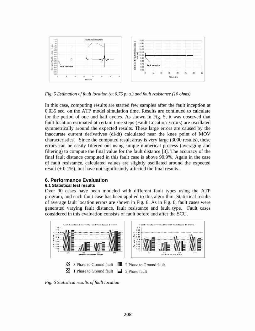
0.400.450.500.550.600.650.700.750.800.850.900.951.001.051.101.151.20
0 5 10 15 20 25 30 35
Time, ms
Estim
ated
Fau
lt Lo
catio
n ( i
n p.
u.)
Fault Inception
Fault Location Errors
9.509.609.709.809.90
10.0010.1010.2010.3010.4010.50
0 5 10 15 20 25 30 35
Time, ms
Estim
ated
Fau
lt R
esis
tanc
e (
ohm
s)
Fault Inception
Fig. 5 Estimation of fault location (at 0.75 p. u.) and fault resistance (10 ohms) In this case, computing results are started few samples after the fault inception at 0.035 sec. on the ATP model simulation time. Results are continued to calculate for the period of one and half cycles. As shown in Fig. 5, it was observed that fault location estimated at certain time steps (Fault Location Errors) are oscillated symmetrically around the expected results. These large errors are caused by the inaccurate current derivatives (di/dt) calculated near the knee point of MOV characteristics. Since the computed result array is very large (3000 results), these errors can be easily filtered out using simple numerical process (averaging and filtering) to compute the final value for the fault distance [8]. The accuracy of the final fault distance computed in this fault case is above 99.9%. Again in the case of fault resistance, calculated values are slightly oscillated around the expected result (± 0.1%), but have not significantly affected the final results. 6. Performance Evaluation 6.1 Statistical test results Over 90 cases have been modeled with different fault types using the ATP program, and each fault case has been applied to this algorithm. Statistical results of average fault location errors are shown in Fig. 6. As in Fig. 6, fault cases were generated varying fault distance, fault resistance and fault type. Fault cases considered in this evaluation consists of fault before and after the SCU.
3 Phase to Ground fault1 Phase to Ground fault
2 Phase to Ground fault2 Phase fault
Fig. 6 Statistical results of fault location
208
6.2 The new algorithm assessment Computed fault location errors are of both positive and negative values. Results shown in Fig. 6 are absolute values round off to two decimals. As shown in Fig. 6, average fault distance estimation considering all fault cases does not exceed 0.2%. In general, according to Fig. 6, fault location estimation error is reduced closer to the middle of the line and this could be due to the result of, offsetting signal measurement and computational errors in local and remote ends of the line. Robustness of this algorithm was tested as follows: Synchronising error is introduced between the local and remote fault currents. It was observed when the synchronising error is less than 0.1ms, fault location error still within ± 0.1%. Variation of source impedance does not show any significant change in the estimation of fault location. This could be as the result of measuring fault signals after the source impedance at local and remote buses [5]. In the case of time varying faults (Varying from 10 ohms to 2.5 ohms in 4 steps during 1.5 cycles after the fault inception), it was observed that this algorithm produced similar accurate results, compared with fixed fault resistance cases [6]. However, the new algorithm stated in this paper is developed using R-L model with, mutual inductances and untransposed phases. In the case of long transmission lines, this algorithm could be modified using travelling wave approach to compute the fault location [8]. 6.3 Comparisons with other fault location algorithms The robustness and flexibility of this algorithm is compared with other time domain [10] and neural network based [11] algorithms in relation to the accuracy of estimating fault location. The time domain fault location algorithm presented by the main authors Javid Sadeh and N. Hadjsaid stated that average fault location error is within 0.5% with compares to proposed fault location error of 0.2%. However, the accuracy of fault location in both algorithms have similar values, proposed algorithm can be implemented in broad range of series compensation devices including TCSC and the algorithm presented by above authors have limitations on this issue. The algorithm used neural network approach [11] has more flexibility in applying to different networks compares to other algorithms, but the accuracy of fault location is highly depends on the level of training data supplied to the algorithm. It can be stated that the proposed algorithm is competitive in accuracy and robustness with other algorithms [10, 11, 2] having limited to short transmission line networks.
209
7. Conclusions The algorithm presented in this paper provides a new accurate method of estimating fault location based on recording instruments assisted with GPS receivers providing accurate synchronised instantaneous fault data from both ends of the series compensated transmission line. Time domain analysis is used in this algorithm, assuming synchronized sample data is available for the estimation fault location accurately. However, the algorithm had been tested for synchronizing error up to 0.1 ms, while maintaining the accuracy (± 0.1%) in fault location. Since the fault location is repeatedly computed using the instantaneous measurements in this algorithm, accuracy of estimation is not affected by the fault resistance, time varying faults, type of SCU except the value of capacitor and source parameters. If the DFRs are not located at each end of the line, one end fault location algorithm [7] proposed by the authors can be applied in most fault cases to estimate the fault location. Finally, it should be pointed out that model in this paper used an R-L model series compensated transmission line with mutual effects. It was concluded that this algorithm can further developed using standing wave approach to employ in long transmission line. 8. References [1] Yu C.H., Liu C.W. “A new PMU- Based Fault Location Algorithm for Series Compensated Lines”, IEEE Transactions on Power Delivery Vol. 17, No.1, January 2002 pp. 33 -46 [2] Saga M.M., Jzykowski J., Rosolowski E. Kasztenny B. “A new accurate fault locating algorithm for series compensated lines”, IEEE Transactions on Power Delivery Vol.14, No. 3, July 1999, pp. 789-795 [3] S. K. Kapuduwage, M. Al-Dabbagh “A New Simplified Fault Location Algorithm for Series Compensated Transmission Lines”, AUPEC 2002, Sep. 2002 [4] M. Al-Dabbagh, S. K. Kapuduwage “A novel Efficient Fault Location Algorithm for series compensated High Voltage Transmission lines”, SCI 2003, July 2003, Vol XIII, pp.20-25 [5] M. Al Dabbagh, S. K. Kapuduwage “A new Method foe Estimating Fault Location on series compensated High Voltage Transmission lines” EuroPES 2004 Power & Energy, Paper ID 442-259, 28-30 June, Rhodes, Greece.
210
[6] M. Al-Dabbagh, S. K. Kapuduwage “Effects of Dynamic Fault Impedance Variation on Accuracy of Fault Location Estimation for Series Compensated Transmission Lines”, WSEAS Conference, Paper ID 489-477, 14-16 Sep. 2004, Izmir, Turkey [7] S. K. Kapuduwage, M. Al-Dabbagh “One End Simplified Fault Location Algorithm Using Instantaneous Values for series compensated High Voltage Transmission Lines, AUPEC 04, Paper ID 23, University Of Queensland, 26 – 29 Sep. 2004 [8] M. Kezunovic, B. Perunicic, J. Mrkic, “An Accurate Fault Location Algorithm Using Synchronized Sampling,” Electric Power Systems Research Journal, Vol. 29, No. 3, pp. 161-169, May 1994 [9] F. Ghassemi, J. Goodarzi A.T. Johns “Method to improve digital distance relay impedance measurement when used in series compensated lines “, IEE Proc., Vol 145, No.4, July 1998 [10] Sadeh, Javad; N. Hadjsaid, "Accurate Fault Location Algorithm for Series Compensated Transmission Lines", IEEE transactions on Power Delivery. [11] Damir Novosal, B. Bachmann, “Algorithms for locating faults on series compensated lines using neural network and deterministic methods” IEEE Transactions on Power Delivery, Vol. 11, No. 4, October 1996 [12] Hewlett Packard Application Note 1276-1 “Accurate Transmission Line Fault Location Using Synchronized Sampling”, June 1996, USA [13] Alternative Transients Program Rule book, 1989 edition
211
A New Simplified Fault Location Algorithm for Series Compensated Transmission Lines
S. K. Kapuduwage, M. Al-Dabbagh Electrical Energy and Control Systems
School of Electrical and Computer Engineering RMIT University – City Campus [email protected]
Abstract This paper presents a new simple fault location algorithm based on measurement of phasor quantities for a two end series compensated transmission lines. The algorithm is developed using linerised model of 3 phase capacitor banks to represent the effects of compensation. Basically, the algorithm uses current and voltage measurements from both ends of the transmission network and accurately estimates the location and the resistance of the fault. The accuracy of the fault location is tested using two-end 300km, 400KV, 3-phase transmission network, modeled using MALAB 6.1 recently developed Power System Block set [1]. The algorithm was implemented using MATLAB programming scripts [1]. The proposed techniques can be easily expanded to adapt multi line, multi end un-transposed transmission lines.
1. INTRODUCTION Transmission of power generated from power plants to consumers have been vastly improved and expanded to every corner of the world during the last two decades. Recent development of series compensation in power systems can greatly increase power transfer capability, damp power oscillations (if carefully designed) and improve the transient stability. However, faults clearing and finding in such transmission networks considered to be one of the most important tasks for the manufactures, operators and maintenance engineers. The basic arrangement of series compensation of a transmission line is a series capacitor(C) and non liner resistor (MOV) in parallel with the capacitor as shown in Fig (1). During a fault, MOV operates as a protection to bypass fault current through the capacitor, which would otherwise cause dangerously high voltage across the capacitor bank. As the series compensation unit is non-liner, fault location can not be determined using traditional impedance measurement techniques. During recent past there have been several improvements to fault finding techniques using phasor-
based approaches [3]; one end and two ends algorithms [4] with satisfactory results. However, these algorithms use direct or indirect measurement of impendence to locate the fault, which would fail in case of series compensated line due to the non-linear operation of the capacitor bank. In order to accommodate the effect of non linearity, current dependent voltage drop across the capacitor is estimated and subtracted from the voltage sources, prior to calculation of distance to the fault. The proposed algorithm uses voltage (V) and current (I) from both ends to accurately estimate the capacitor voltage drop in order to calculate distance to the fault in event of fault occurs before or after the series compensation unit. Availability of measurement of V and I of both ends allow source impendence to be estimated more accurately and hence improve the accuracy of the fault location and simplify the calculation algorithm. The proposed algorithm has been tested with wide selections of faults; fault type, fault location and angle of inception, using MATLAB 6.1. Firstly the transmission network is modeled and simulated with power system block set of MATLAB [1] and simulated output data ( voltage and currents from sending and receiving end ) are fed to the new algorithm
1 212
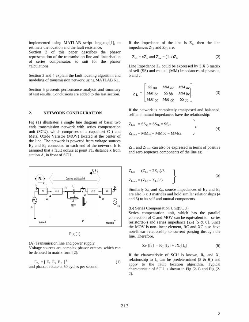
implemented using MATLAB script language[1], to estimate the location and the fault resistance. Section 2 of this paper describes the phasor representation of the transmission line and linearisation of series compensator, to suit for the phasor calculations. Section 3 and 4 explain the fault locating algorithm and modeling of transmission network using MATLAB 6.1. Section 5 presents performance analysis and summary of test results. Conclusions are added to the last section. 2. NETWORK CONFIGURATION Fig (1) illustrates a single line diagram of basic two ends transmission network with series compensation unit (SCU), which comprises of a capacitor( C ) and Metal Oxide Varistor (MOV) located at the center of the line. The network is powered from voltage sources EA and EB connected to each end of the network. It is assumed that a fault occurs at point F1, distance x from station A, in front of SCU.
EA
Station A
ZA ZL1 ZL2 ZB
MOV
C
EB
VF
F2IA IB
IFVA VB
F1
Station B
Controls and Data linkFL
VB & IB
Fig (1)
(A) Transmission line and power supply Voltage sources are complex phasor vectors, which can be denoted in matrix form [2]:
EA = [ Ea Eb Ec ] T (1) and phasors rotate at 50 cycles per second.
If the impedance of the line is ZL, then the line impedances ZL1 and ZL2 are:
ZL1 = xZL and ZL2 = (1-x)ZL (2) Line Impedance ZL could be expressed by 3 X 3 matrix of self (SS) and mutual (MM) impedances of phases a, b and c:
⎥⎥
⎦
⎤
⎢⎢
⎣
⎡=
SS ccMM cbMM ca
MM bcSS bbMM ba
MM acMM abSS aaZ L (3)
If the network is completely transposed and balanced, self and mutual impedances have the relationship: ZLss = SSaa = SSbb = SScc
(4) ZLmm = MMab = MMbc = MMca ZLss and ZLmm can also be expressed in terms of positive and zero sequence components of the line as; ZLss = (ZL0 + 2ZL+)/3
(5) ZLmm = (ZL0 – XL+)/3 Similarly ZA and ZB, source impedances of EA and EB are also 3 x 3 matrices and hold similar relationships (4 and 5) to its self and mutual components. (B) Series Compensation Unit(SCU) Series compensation unit, which has the parallel connection of C and MOV can be equivalent to series resistor(RC) and series impedance (ZC) [5 & 6]. Since the MOV is non-linear element, RC and XC also have non-linear relationship to current passing through the line. Therefore,
Zv [IA] = RC [IA] + JXC[IA] (6) If the characteristic of SCU is known, RC and XC relationship to IA can be predetermined [5 & 6]) and apply to the fault location algorithm. Typical characteristic of SCU is shown in Fig (2-1) and Fig (2-2).
2 213
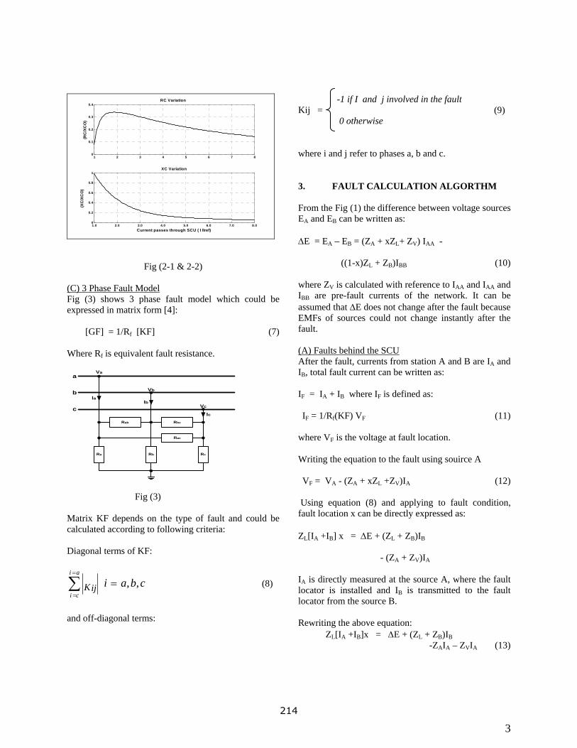
1 2 3 4 5 6 7 80
0.1
0.2
0.3
0.4
(RC
/XC
O)
RC Variation
1.0 2.0 3.0 4.0 5.0 6.0 7.0 8.00
0.2
0.4
0.6
0.8
1
Current passes through SCU ( I /Iref)
(XC
/XC
O)
XC Variation
Fig (2-1 & 2-2) (C) 3 Phase Fault Model Fig (3) shows 3 phase fault model which could be expressed in matrix form [4]:
[GF] = 1/Rf [KF] (7) Where Rf is equivalent fault resistance.
Rab Rbc
Rac
Ra Rb Rc
Va
Vb
Vc
IaIb
Ic
a
b
c
Fig (3)
Matrix KF depends on the type of fault and could be calculated according to following criteria: Diagonal terms of KF:
cbaiai
ciKij ,,=∑
=
=
(8)
and off-diagonal terms:
-1 if I and j involved in the fault Kij = (9) 0 otherwise where i and j refer to phases a, b and c. 3. FAULT CALCULATION ALGORTHM From the Fig (1) the difference between voltage sources EA and EB can be written as: ∆E = EA – EB = (ZA + xZL+ ZV) IAA -
((1-x)ZL + ZB)IBB (10) where ZV is calculated with reference to IAA and IAA and IBB are pre-fault currents of the network. It can be assumed that ∆E does not change after the fault because EMFs of sources could not change instantly after the fault. (A) Faults behind the SCU After the fault, currents from station A and B are IA and IB, total fault current can be written as: IF = IA + IB where IF is defined as: IF = 1/Rf(KF) VF (11)
where VF is the voltage at fault location. Writing the equation to the fault using souirce A VF = VA - (ZA + xZL +ZV)IA (12)
Using equation (8) and applying to fault condition, fault location x can be directly expressed as: ZL[IA +IB] x = ∆E + (ZL + ZB)IB - (ZA + ZV)IA IA is directly measured at the source A, where the fault locator is installed and IB is transmitted to the fault locator from the source B. Rewriting the above equation:
ZL[IA +IB]x = ∆E + (ZL + ZB)IB -ZAIA – ZVIA (13)
3 214
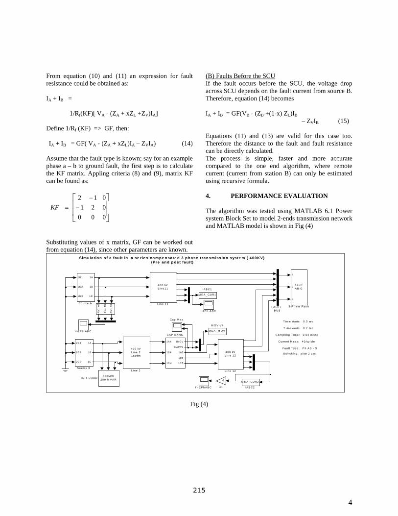
(B) Faults Before the SCU From equation (10) and (11) an expression for fault
resistance could be obtained as: If the fault occurs before the SCU, the voltage drop across SCU depends on the fault current from source B. Therefore, equation (14) becomes
IA + IB = 1/Rf(KF)[ VA - (ZA + xZL +ZV)IA] IA + IB = GF(VB - (ZB +(1-x) ZL)IB
– ZVIB (15) Define 1/Rf (KF) => GF, then: Equations (11) and (13) are valid for this case too. Therefore the distance to the fault and fault resistance can be directly calculated.
IA + IB = GF( VA - (ZA + xZL)IA – ZVIA) (14)
Assume that the fault type is known; say for an example phase a – b to ground fault, the first step is to calculate the KF matrix. Appling criteria (8) and (9), matrix KF can be found as:
The process is simple, faster and more accurate compared to the one end algorithm, where remote current (current from station B) can only be estimated using recursive formula.
4. PERFORMANCE EVALUATION
⎥⎥
⎦
⎤
⎢⎢
⎣
⎡−
−=
000021012
KF The algorithm was tested using MATLAB 6.1 Power system Block Set to model 2-ends transmission network and MATLAB model is shown in Fig (4) Substituting values of x matrix, GF can be worked out
from equation (14), since other parameters are known. Simu latio n o f a fau lt in a se r ie s co mp e n sate d 3 p h ase tran smissio n syste m ( 400KV)
(Pre an d p o st fau lt)
S a m p l in g T im e : 0 .0 2 m se c
T im e sta rts: 0 .0 se c
T im e e n d s: 0 .2 se c
Cu rre n t M e a s: 4 0 /cyl c le
Fa u l t T yp e : P h A B - G
S wi tch in g : a fte r 2 cyc.
A1 B1 C1
AV1
BV1
CV1
V -1 P h A B C
2G 1
2G 2
2G 3
1A
1B
1C
S o u rce B
1G 1
1G 2
1G 3
1A
1B
1C
S o u rce A
M E A _ M O V
M O V -V I
4 0 0 kVL in e 21 5 0 km
L in e 2
4 0 0 kVL i n e 1 2
L i n e 1 2
4 0 0 kVL in e 1 1
L in e 1 1
3 0 0 M W2 8 0 M V A RINIT L O A D
M E A _ CUR2
IA B C2
M E A _ CUR1
IA B C1
I-1 P h A B C
I - 2 P h A B C
-1
G 1
1
1
1
2
2
2
2
2
3
FA UL T B US
Ca p M e a
1A4
1B4
1C 4
IMO V
C APV1
1A5
1B5
1C 5
CA P B A NK
A
B
C
Fa u l tA B -G
3 -P h a se Fa u l t
Fig (4)
4 215
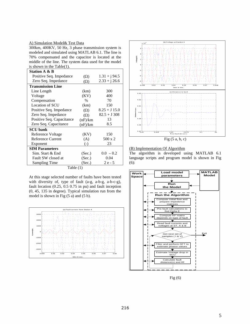
A) Simulation Model& Test Data 300km, 400KV, 50 Hz, 3 phase transmission system is modeled and simulated using MATLAB 6.1. The line is 70% compensated and the capacitor is located at the middle of the line. The system data used for the model is shown in the Table(1). Station A & B Positive Seq. Impedance Zero Seq. Impedance
(Ω) (Ω)
1.31 + j 94.5 2.33 + j 26.6
Transmission Line Line Length Voltage Compensation Location of SCU Positive Seq. Impedance Zero Seq. Impedance Positive Seq. Capacitance Zero Seq. Capacitance
(km) (KV)
% (km) (Ω) (Ω)
(nF)/km (nF)/km
300 400 70 150
8.25 + J 15.0 82.5 + J 308
13 8.5
SCU bank Reference Voltage Reference Current Exponent
(KV) (A) (-)
150
500 x 2 23
SIM Parameters Sim. Start & End Fault SW closed at Sampling Time
(Sec.) (Sec.) (Sec.)
0.0 – 0.2
0.04 2 e - 5
Table (1) At this stage selected number of faults have been tested with diversity of, type of fault (a-g, a-b-g, a-b-c-g), fault location (0.25, 0.5 0.75 in pu) and fault inception (0, 45, 135 in degree). Typical simulation run from the model is shown in Fig (5 a) and (5 b).
0 .0 0 8 0 .0 2 0 .0 3 0 .0 4 0 .0 5 0 .0 6 0 .0 7 0 .0 8
-3 0 0 0
-2 0 0 0
-1 0 0 0
0
1 0 0 0
2 0 0 0
3 0 0 0
tim e in s e c .
Cur
rent
(A)
( a ) F a u lt c u r re n t- fro m S ta t io n A
0 .0 0 8 0 .0 2 0 .0 3 0 .0 4 0 .0 5 0 .0 6 0 .0 7 0 .0 0 8
-3
-2
-1
0
1
2
3
x 1 05
t im e in s e c .
Volta
ge(V
)
( b ) V o lta g e a t S ta t io n A
0 .0 2 0 .0 2 5 0 .0 5 0 .0 7 5 0 .1 2 50 .4 7
0 .4 8
0 .4 9
0 .5
0 .5 1
0 .5 2
0 .5 3
P o s t f a u lt ( in s e c .)D
ista
nce
in p
.u.
( c ) D is t a n c e t o f a u lt
Fig (5 a, b, c)
(B) Implementation Of Algorithm The algorithm is developed using MATLAB 6.1 language scripts and program model is shown in Fig (6):
Load modelparameters
WorkSpace
MATLABModel
Runthe Model
Run the Algorithm
Get next set ofsamples ( I & V)
Compute initial flow andprepare impedence
matrices
Pre-fault calculations tofind Delta E
Compute KF matrixdepends on type of fault
Read fault currents andvottages at ST. A & B
Filter and perform DFT toestimate phasor values
Estimate Vottage drop inSCU
Calculate faultdistance(x) and Rf
Exit
Fig (6)
5 216
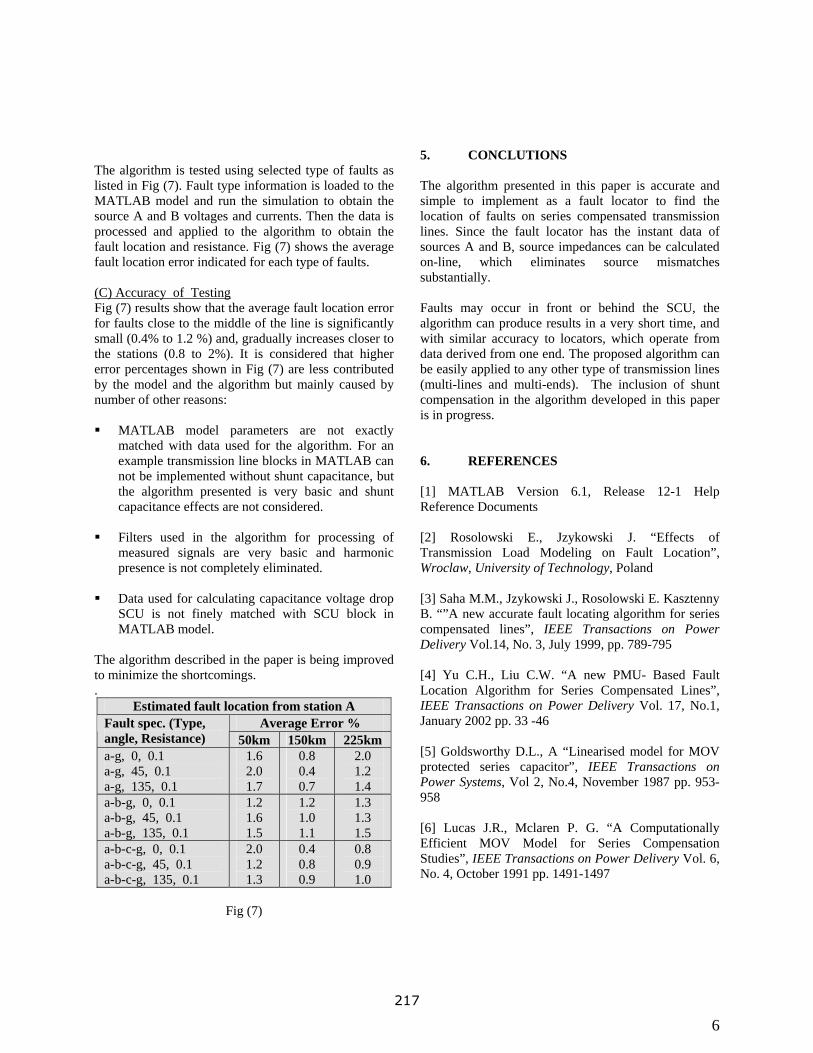
The algorithm is tested using selected type of faults as listed in Fig (7). Fault type information is loaded to the MATLAB model and run the simulation to obtain the source A and B voltages and currents. Then the data is processed and applied to the algorithm to obtain the fault location and resistance. Fig (7) shows the average fault location error indicated for each type of faults. (C) Accuracy of Testing Fig (7) results show that the average fault location error for faults close to the middle of the line is significantly small (0.4% to 1.2 %) and, gradually increases closer to the stations (0.8 to 2%). It is considered that higher error percentages shown in Fig (7) are less contributed by the model and the algorithm but mainly caused by number of other reasons: MATLAB model parameters are not exactly
matched with data used for the algorithm. For an example transmission line blocks in MATLAB can not be implemented without shunt capacitance, but the algorithm presented is very basic and shunt capacitance effects are not considered.
Filters used in the algorithm for processing of
measured signals are very basic and harmonic presence is not completely eliminated.
Data used for calculating capacitance voltage drop
SCU is not finely matched with SCU block in MATLAB model.
The algorithm described in the paper is being improved to minimize the shortcomings. .
Estimated fault location from station A Average Error % Fault spec. (Type,
angle, Resistance) 50km 150km 225km a-g, 0, 0.1 a-g, 45, 0.1 a-g, 135, 0.1
1.6 2.0 1.7
0.8 0.4 0.7
2.0 1.2 1.4
a-b-g, 0, 0.1 a-b-g, 45, 0.1 a-b-g, 135, 0.1
1.2 1.6 1.5
1.2 1.0 1.1
1.3 1.3 1.5
a-b-c-g, 0, 0.1 a-b-c-g, 45, 0.1 a-b-c-g, 135, 0.1
2.0 1.2 1.3
0.4 0.8 0.9
0.8 0.9 1.0
Fig (7)
5. CONCLUTIONS
The algorithm presented in this paper is accurate and simple to implement as a fault locator to find the location of faults on series compensated transmission lines. Since the fault locator has the instant data of sources A and B, source impedances can be calculated on-line, which eliminates source mismatches substantially. Faults may occur in front or behind the SCU, the algorithm can produce results in a very short time, and with similar accuracy to locators, which operate from data derived from one end. The proposed algorithm can be easily applied to any other type of transmission lines (multi-lines and multi-ends). The inclusion of shunt compensation in the algorithm developed in this paper is in progress. 6. REFERENCES
[1] MATLAB Version 6.1, Release 12-1 Help Reference Documents [2] Rosolowski E., Jzykowski J. “Effects of Transmission Load Modeling on Fault Location”, Wroclaw, University of Technology, Poland [3] Saha M.M., Jzykowski J., Rosolowski E. Kasztenny B. “”A new accurate fault locating algorithm for series compensated lines”, IEEE Transactions on Power Delivery Vol.14, No. 3, July 1999, pp. 789-795 [4] Yu C.H., Liu C.W. “A new PMU- Based Fault Location Algorithm for Series Compensated Lines”, IEEE Transactions on Power Delivery Vol. 17, No.1, January 2002 pp. 33 -46 [5] Goldsworthy D.L., A “Linearised model for MOV protected series capacitor”, IEEE Transactions on Power Systems, Vol 2, No.4, November 1987 pp. 953-958 [6] Lucas J.R., Mclaren P. G. “A Computationally Efficient MOV Model for Series Compensation Studies”, IEEE Transactions on Power Delivery Vol. 6, No. 4, October 1991 pp. 1491-1497
6 217
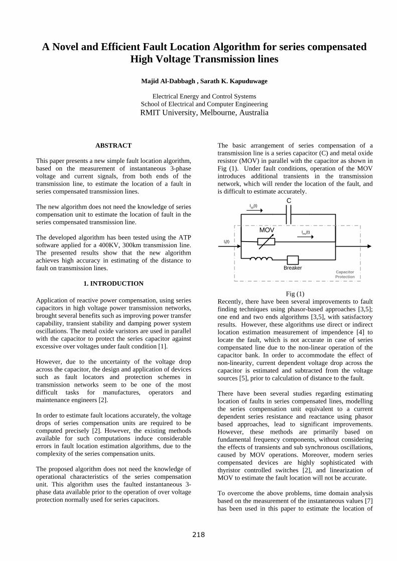
A Novel and Efficient Fault Location Algorithm for series compensated
High Voltage Transmission lines
Majid Al-Dabbagh , Sarath K. Kapuduwage
Electrical Energy and Control Systems School of Electrical and Computer Engineering RMIT University, Melbourne, Australia
ABSTRACT This paper presents a new simple fault location algorithm, based on the measurement of instantaneous 3-phase voltage and current signals, from both ends of the transmission line, to estimate the location of a fault in series compensated transmission lines. The new algorithm does not need the knowledge of series compensation unit to estimate the location of fault in the series compensated transmission line. The developed algorithm has been tested using the ATP software applied for a 400KV, 300km transmission line. The presented results show that the new algorithm achieves high accuracy in estimating of the distance to fault on transmission lines.
1. INTRODUCTION Application of reactive power compensation, using series capacitors in high voltage power transmission networks, brought several benefits such as improving power transfer capability, transient stability and damping power system oscillations. The metal oxide varistors are used in parallel with the capacitor to protect the series capacitor against excessive over voltages under fault condition [1]. However, due to the uncertainty of the voltage drop across the capacitor, the design and application of devices such as fault locators and protection schemes in transmission networks seem to be one of the most difficult tasks for manufactures, operators and maintenance engineers [2]. In order to estimate fault locations accurately, the voltage drops of series compensation units are required to be computed precisely [2]. However, the existing methods available for such computations induce considerable errors in fault location estimation algorithms, due to the complexity of the series compensation units. The proposed algorithm does not need the knowledge of operational characteristics of the series compensation unit. This algorithm uses the faulted instantaneous 3-phase data available prior to the operation of over voltage protection normally used for series capacitors.
The basic arrangement of series compensation of a transmission line is a series capacitor (C) and metal oxide resistor (MOV) in parallel with the capacitor as shown in Fig (1). Under fault conditions, operation of the MOV introduces additional transients in the transmission network, which will render the location of the fault, and is difficult to estimate accurately.
C
MOV
BreakerCapacitorProtection
If(t)
Icp(t)
Imv(t)
Fig (1) Recently, there have been several improvements to fault finding techniques using phasor-based approaches [3,5]; one end and two ends algorithms [3,5], with satisfactory results. However, these algorithms use direct or indirect location estimation measurement of impendence [4] to locate the fault, which is not accurate in case of series compensated line due to the non-linear operation of the capacitor bank. In order to accommodate the effect of non-linearity, current dependent voltage drop across the capacitor is estimated and subtracted from the voltage sources [5], prior to calculation of distance to the fault. There have been several studies regarding estimating location of faults in series compensated lines, modelling the series compensation unit equivalent to a current dependent series resistance and reactance using phasor based approaches, lead to significant improvements. However, these methods are primarily based on fundamental frequency components, without considering the effects of transients and sub synchronous oscillations, caused by MOV operations. Moreover, modern series compensated devices are highly sophisticated with thyristor controlled switches [2], and linearization of MOV to estimate the fault location will not be accurate. To overcome the above problems, time domain analysis based on the measurement of the instantaneous values [7] has been used in this paper to estimate the location of
218
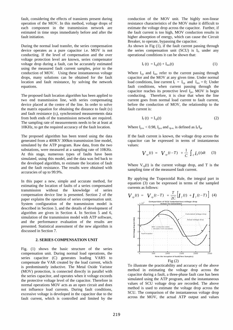
fault, considering the effects of transients present during operation of the MOV. In this method, voltage drops of each component in the transmission network are estimated in time steps immediately before and after the fault initiation. During the normal load transfer, the series compensation device operates as a pure capacitor i.e. MOV is not conducting. If the level of compensation and the over voltage protection level are known, series compensator voltage drop during a fault, can be accurately estimated using the measured fault current samples, prior to the conduction of MOV. Using these instantaneous voltage drops, many solutions can be obtained for the fault location and fault resistance, by solving the network equations. The proposed fault location algorithm has been applied to two end transmission line, with series compensating device placed at the centre of the line. In order to solve the matrix equation for obtaining the distance to fault (x) and fault resistance (rf), synchronised measurements data from both ends of the transmission network are required. The sampling rate of measurements needs to be at least at 10KHz, to get the required accuracy of the fault location. The proposed algorithm has been tested using the data generated from a 400KV 300km transmission line model, simulated by the ATP program. Raw data, from the two substations, were measured at a sampling rate of 10KHz. At this stage, numerous types of faults have been simulated, using this model, and the data was fed back to the developed algorithm, to estimate the location of fault and the fault resistance. The results were obtained with accuracies of up to 99.9%. In this paper a new, simple and accurate method, for estimating the location of faults of a series compensated transmission without the knowledge of series compensation device line is presented. Section 2 of the paper explains the operation of series compensation unit. System configuration of the transmission model is described in Section 3, and the details of development of algorithm are given in Section 4. In Section 5 and 6, simulation of the transmission model with ATP software, and the performance evaluation of the results are presented. Statistical assessment of the new algorithm is discussed in Section 7.
2. SERIES COMPENSATION UNIT
Fig. (1) shows the basic structure of the series compensation unit. During normal load operations, the series capacitor (C) generates leading VARS to compensate the VAR created by the load current, which is predominately inductive. The Metal Oxide Varistor (MOV) protection, is connected directly in parallel with the series capacitor, and operates when it voltage exceeds the protective voltage level of the capacitor. Therefore in normal operations MOV acts as an open circuit and does not influence load currents. During fault conditions, excessive voltage is developed in the capacitor due to the fault current, which is controlled and limited by the
conduction of the MOV unit. The highly non-linear resistance characteristics of the MOV make it difficult to estimate the voltage drop across the capacitor. Further, if the fault current is too high, MOV conduction results in higher absorption of energy, which can cause the Circuit Breaker, to operate, bypassing the capacitor. As shown in Fig (1), if the fault current passing through the series compensation unit (SCU) is If, under any operational conditions it can be shown that:
If (t) = Icp(t) + Imv(t) (1) Where Icp and Imv refer to the current passing through capacitor and the MOV at any given time. Under normal load conditions, line current Il = Icp and Imv = 0; Under fault conditions, when current passing through the capacitor reaches its protective level Ipr, MOV is begin conducting. Therefore, it is clear that when the line current goes from normal load current to fault current, before the conduction of MOV, the relationship to the fault current is: If (t) = Icp(t) (2) Where Ip.u. < 0.98, Ip.u and Ip.u. is defined as If/Ipr
If the fault current is known, the voltage drop across the capacitor can be expressed in terms of instantaneous values:
dttC
Tttt
Tt Fcpcp iVV )(1)()( ∫ −+−= (3)
Where Vcp(t) is the current voltage drop, and T is the sampling time of the measured fault current. By applying the Trapezoidal Rule, the integral part in equation (3) can be expressed in terms of the sampled currents as follows:
[ ])()(2
)()( TttCTTtt IIVV ffcpcp −++−= (4)
0 500 1000 1500 2000 2500-8
-6
-4
-2
0
2
4
6x 10⁵
Form the inc e ption of fa ult(Tim e S a m ple s )
SCU
Vot
age
Dro
p (in
Vol
ts)
Actu a l vo lta g e d ro p
C a lcu la te d vo lta g e d ro p
MOV c onduc tion s tar ts ( dev ia tes f rom c ac u la ted)
Fault inc eption
Co m pa rision o f S CU insta n ta n ious vo lta ge drop Actua l V s Ca lcu la te d
Fig (2)
To illustrate the practicability and accuracy of the above method in estimating the voltage drop across the capacitor during a fault, a three-phase fault case has been simulated using the ATP program, and the instantaneous values of SCU voltage drop are recorded. The above method is used to estimate the voltage drop across the SCU. The comparison of the instantaneous voltage drop across the MOV, the actual ATP output and values
219
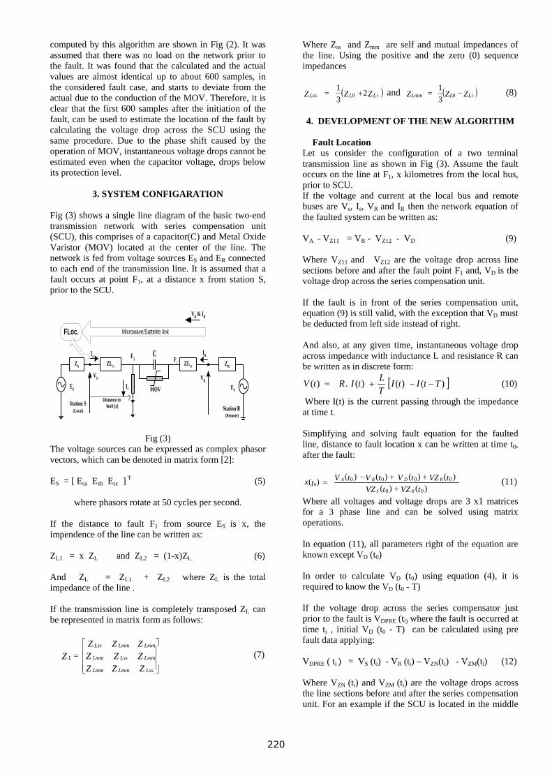
computed by this algorithm are shown in Fig (2). It was assumed that there was no load on the network prior to the fault. It was found that the calculated and the actual values are almost identical up to about 600 samples, in the considered fault case, and starts to deviate from the actual due to the conduction of the MOV. Therefore, it is clear that the first 600 samples after the initiation of the fault, can be used to estimate the location of the fault by calculating the voltage drop across the SCU using the same procedure. Due to the phase shift caused by the operation of MOV, instantaneous voltage drops cannot be estimated even when the capacitor voltage, drops below its protection level.
3. SYSTEM CONFIGARATION Fig (3) shows a single line diagram of the basic two-end transmission network with series compensation unit (SCU), this comprises of a capacitor(C) and Metal Oxide Varistor (MOV) located at the center of the line. The network is fed from voltage sources ES and ER connected to each end of the transmission line. It is assumed that a fault occurs at point F1, at a distance x from station S, prior to the SCU.
FLoc.
ES
Station S(Local)
ZS ZL11 ZL22 ZR
MOV
C
ER
F2
ISIR
IF
VS VR
Station R(Remote)
VR & IR
Microwave/Sattelite link
F1
Distance to fault (x)
Fig (3) The voltage sources can be expressed as complex phasor vectors, which can be denoted in matrix form [2]: ES = [ Esa Esb Esc ] T (5)
where phasors rotate at 50 cycles per second. If the distance to fault F1 from source ES is x, the impendence of the line can be written as: ZL1 = x ZL and ZL2 = (1-x)ZL (6) And ZL = ZL1 + ZL2 where ZL is the total impedance of the line . If the transmission line is completely transposed ZL can be represented in matrix form as follows:
(7) ⎥⎥⎥
⎦
⎤
⎢⎢⎢
⎣
⎡=
ZZZZZZZZZ
ZLssLmmLmm
LmmLssLmm
LmmLmmLss
L
Where Zss and Zmm are self and mutual impedances of the line. Using the positive and the zero (0) sequence impedances
( )ZZZ LLLss ++= 231
0 and ( ) (8) ZZZ LLLmm +−= 031
4. DEVELOPMENT OF THE NEW ALGORITHM
Fault Location
Let us consider the configuration of a two terminal transmission line as shown in Fig (3). Assume the fault occurs on the line at F1, x kilometres from the local bus, prior to SCU. If the voltage and current at the local bus and remote buses are Vs, Is, VR and IR then the network equation of the faulted system can be written as: VA - VZ11 = VB - VZ12 - VD (9) Where VZ11 and VZ12 are the voltage drop across line sections before and after the fault point F1 and, VD is the voltage drop across the series compensation unit. If the fault is in front of the series compensation unit, equation (9) is still valid, with the exception that VD must be deducted from left side instead of right. And also, at any given time, instantaneous voltage drop across impedance with inductance L and resistance R can be written as in discrete form:
[ )()()(.)( TtItI ]TLtIRtV −−+= (10)
Where I(t) is the current passing through the impedance at time t. Simplifying and solving fault equation for the faulted line, distance to fault location x can be written at time t0, after the fault:
)()()()()()()(
00
00000
tVZtVZtVZtVtVtVtx
RS
RDBA
+++−
= (11)
Where all voltages and voltage drops are 3 x1 matrices for a 3 phase line and can be solved using matrix operations. In equation (11), all parameters right of the equation are known except VD (t0) In order to calculate VD (t0) using equation (4), it is required to know the VD (t0 - T) If the voltage drop across the series compensator just prior to the fault is VDPRE (ti) where the fault is occurred at time ti , initial VD (t0 - T) can be calculated using pre fault data applying: VDPRE ( ti ) = VS (ti) - VR (ti) – VZN(ti) - VZM(ti) (12) Where VZN (ti) and VZM (ti) are the voltage drops across the line sections before and after the series compensation unit. For an example if the SCU is located in the middle
220
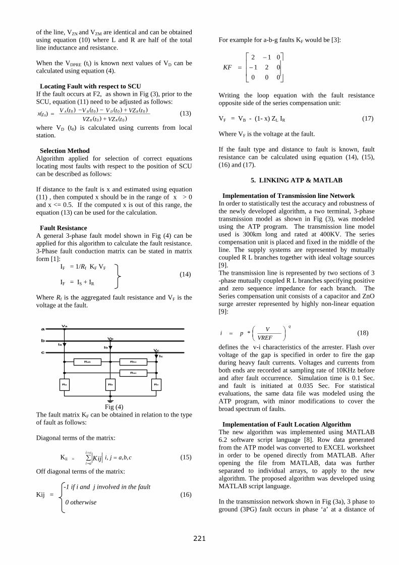
of the line, VZN and VZM are identical and can be obtained using equation (10) where L and R are half of the total line inductance and resistance. When the VDPRE (ti) is known next values of VD can be calculated using equation (4).
Locating Fault with respect to SCU If the fault occurs at F2, as shown in Fig (3), prior to the SCU, equation (11) need to be adjusted as follows:
)()()()()()()(
00
00000
tVZtVZtVZtVtVtVtx
RR
RDBA
++−−
= (13)
where VD (t0) is calculated using currents from local station.
Selection Method Algorithm applied for selection of correct equations locating most faults with respect to the position of SCU can be described as follows: If distance to the fault is x and estimated using equation (11) , then computed x should be in the range of x > 0 and x <= 0.5. If the computed x is out of this range, the equation (13) can be used for the calculation.
Fault Resistance A general 3-phase fault model shown in Fig (4) can be applied for this algorithm to calculate the fault resistance. 3-Phase fault conduction matrix can be stated in matrix form [1]: IF = 1/Rf KF VF (14) IF = IS + IR Where Rf is the aggregated fault resistance and VF is the voltage at the fault.
Rab Rbc
Rac
Ra Rb Rc
Va
Vb
Vc
IaIb
Ic
a
b
c
Fig (4)
The fault matrix KF can be obtained in relation to the type of fault as follows: Diagonal terms of the matrix:
Kii = cbajici
aiKij ,,, =∑
=
= (15)
Off diagonal terms of the matrix: -1 if i and j involved in the fault Kij = (16) 0 otherwise
For example for a-b-g faults KF would be [3]:
⎥⎥
⎦
⎤
⎢⎢
⎣
⎡−
−=
000021012
KF
Writing the loop equation with the fault resistance opposite side of the series compensation unit: VF = VB - (1- x) ZL IR (17) Where VF is the voltage at the fault. If the fault type and distance to fault is known, fault resistance can be calculated using equation (14), (15), (16) and (17).
5. LINKING ATP & MATLAB
Implementation of Transmission line Network In order to statistically test the accuracy and robustness of the newly developed algorithm, a two terminal, 3-phase transmission model as shown in Fig (3), was modeled using the ATP program. The transmission line model used is 300km long and rated at 400KV. The series compensation unit is placed and fixed in the middle of the line. The supply systems are represented by mutually coupled R L branches together with ideal voltage sources [9]. The transmission line is represented by two sections of 3 -phase mutually coupled R L branches specifying positive and zero sequence impedance for each branch. The Series compensation unit consists of a capacitor and ZnO surge arrester represented by highly non-linear equation [9]:
⎟⎠⎞
⎜⎝⎛=
VREFVpi
q
* (18)
defines the v-i characteristics of the arrester. Flash over voltage of the gap is specified in order to fire the gap during heavy fault currents. Voltages and currents from both ends are recorded at sampling rate of 10KHz before and after fault occurrence. Simulation time is 0.1 Sec. and fault is initiated at 0.035 Sec. For statistical evaluations, the same data file was modeled using the ATP program, with minor modifications to cover the broad spectrum of faults.
Implementation of Fault Location Algorithm The new algorithm was implemented using MATLAB 6.2 software script language [8]. Row data generated from the ATP model was converted to EXCEL worksheet in order to be opened directly from MATLAB. After opening the file from MATLAB, data was further separated to individual arrays, to apply to the new algorithm. The proposed algorithm was developed using MATLAB script language. In the transmission network shown in Fig (3a), 3 phase to ground (3PG) fault occurs in phase ‘a’ at a distance of
221
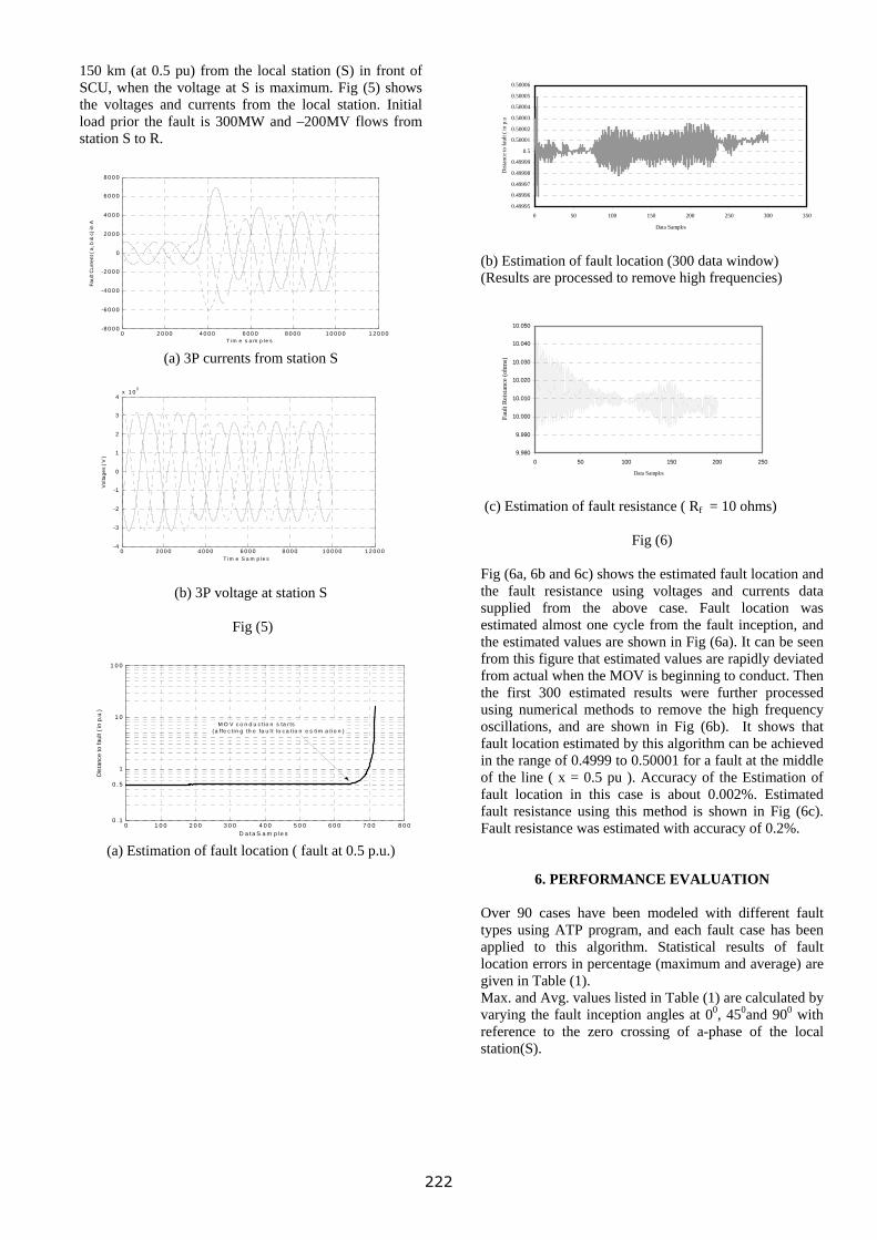
150 km (at 0.5 pu) from the local station (S) in front of SCU, when the voltage at S is maximum. Fig (5) shows the voltages and currents from the local station. Initial load prior the fault is 300MW and –200MV flows from station S to R.
0 2 0 0 0 4 0 0 0 6 0 0 0 8 0 0 0 1 0 0 0 0 1 2 0 0 0-8 0 0 0
-6 0 0 0
-4 0 0 0
-2 0 0 0
0
2 0 0 0
4 0 0 0
6 0 0 0
8 0 0 0
T im e s a m p le s
Faul
t Cur
rent
( a,
b &
c) i
n A
(a) 3P currents from station S
0 2 0 0 0 4 0 0 0 6 0 0 0 8 0 0 0 1 0 0 0 0 1 2 0 0 0-4
-3
-2
-1
0
1
2
3
4x 1 0 5
T im e S a m p le s
Vol
tage
s ( V
)
(b) 3P voltage at station S
Fig (5)
0 1 0 0 2 0 0 3 0 0 4 0 0 5 0 0 6 0 0 7 0 0 8 0 00 . 1
0 . 5
1
1 0
1 0 0
D a t a S a m p le s
Dis
tanc
e to
faul
t ( in
p.u
.)
M O V c o n d u c ti o n s ta r ts ( a ffe c ti n g th e fa u l t l o c a ti o n e s tim a ti o n )
(a) Estimation of fault location ( fault at 0.5 p.u.)
0.49995
0.49996
0.49997
0.49998
0.49999
0.5
0.50001
0.50002
0.50003
0.50004
0.50005
0.50006
0 50 100 150 200 250 300 350
Data Samples
Dis
tanc
e to
faul
t ( in
p.u
(b) Estimation of fault location (300 data window) (Results are processed to remove high frequencies)
9.980
9.990
10.000
10.010
10.020
10.030
10.040
10.050
0 50 100 150 200 250
Data Samples
Faul
t Rei
stan
ce (o
hms)
(c) Estimation of fault resistance ( Rf = 10 ohms)
Fig (6) Fig (6a, 6b and 6c) shows the estimated fault location and the fault resistance using voltages and currents data supplied from the above case. Fault location was estimated almost one cycle from the fault inception, and the estimated values are shown in Fig (6a). It can be seen from this figure that estimated values are rapidly deviated from actual when the MOV is beginning to conduct. Then the first 300 estimated results were further processed using numerical methods to remove the high frequency oscillations, and are shown in Fig (6b). It shows that fault location estimated by this algorithm can be achieved in the range of 0.4999 to 0.50001 for a fault at the middle of the line ( x = 0.5 pu ). Accuracy of the Estimation of fault location in this case is about 0.002%. Estimated fault resistance using this method is shown in Fig (6c). Fault resistance was estimated with accuracy of 0.2%.
6. PERFORMANCE EVALUATION Over 90 cases have been modeled with different fault types using ATP program, and each fault case has been applied to this algorithm. Statistical results of fault location errors in percentage (maximum and average) are given in Table (1). Max. and Avg. values listed in Table (1) are calculated by varying the fault inception angles at 00, 450and 900 with reference to the zero crossing of a-phase of the local station(S).
222
Table (1)
7. ALGORITHM ASSESMENT
Table (1) shows that largest average fault location error, considering all possible fault cases using this method, is about 0.07%, which is very accurate compared to the most of other methods [2,3,5] proposed by other authors. For an example, if the transmission line is 300km as it was in this model, location of a fault can be estimated within 200m. (An error of 0.07%) It was also observed that fault resistance estimated using this algorithm is about 0.1%. The fault location error is increased in low resistance cases with higher levels of harmonics. Since the effect of MOV is not taken into consideration of estimating the fault location, unlike in other algorithms, fault in prior or after the SCU do not affect the accuracy. If the level of compensation is remained the same during the fault, similar accuracies can be obtained irrespective of how complicated the MOV operation. [2] (For an example, lines incorporated with Thyristor Controlled Series Compensators) However the presented algorithm requires synchronized measurement of voltages and currents from both ends of the transmission line before and after the fault for a very short period ( less than ½ cycles after the fault.)
8. CONCLUSIONS
A new, accurate and robust algorithm for estimating the fault location on series compensated transmission lines is presented. The proposed algorithm does not utilize the type of SCU and knowledge of the operation characteristics of the device to compute the voltage drops during the fault.
Designing the fault locator using this algorithm is not a complicated task compared to other methods in which, accurate details of SCU are critical to achieve the accuracy of fault estimation. Further, this algorithm does not require the fault to be pure resistive or the knowledge of fault type in order to implement successfully. However, the knowledge of fault type is required to estimate the fault resistance. The high frequency components in fault waveforms present inaccuracies in most fault location algorithms. Since the proposed algorithm is based on instantaneous values of measurements, there is no need for filtering high frequencies before applying it. In most of the fault cases carried out, the overall accuracy of estimating the fault location on series compensated two ends lines using this algorithm exceeds 99.9%.
9 REFERENCES [1] Rosolowski E., Jzykowski J. “Effects of Transmission Load Modelling on Fault Location”, Wroclaw, University of Technology, Poland [2] Yu C.H., Liu C.W. “A new PMU- Based Fault Location Algorithm for Series Compensated Lines”, IEEE Transactions on Power Delivery Vol. 17, No.1, January 2002 pp. 33 -46 [3] Saha M.M., Jzykowski J., Rosolowski E. Kasztenny B. “A new accurate fault locating algorithm for series compensated lines”, IEEE Transactions on Power Delivery Vol.14, No. 3, July 1999, pp. 789-795 [4] A.T. Jones, P.J.Moore, R. Whittard “New technique for the accurate location of earth faults on transmission systems”, IEE Proc., Vol142, No.2, March 1995 [5] S. K. Kapuduwage, M. Al-Dabbagh “A New Simplified Fault Location Algorithm for Series Compensated Transmission Lines”, AUPEC 2002, Sep. 2002 [6] Goldsworthy D.L., “ A Linearised model for MOV protected series capacitor”, IEEE Transactions on Power Systems, Vol 2, No.4, November 1987 pp. 953-958 [7] F. Ghassemi J. Goodarzi A.T. Johns “Method to improve digital distance relay impedance measurement when used in series compensated lines protected by a metal oxide varistor “, IEE Proc., Vol145, No.4, July 1998 [8] MATLAB Version 6.1, Release 12-1 Help Reference Documents [9] Alternative Transients Program Rule book, 1989 edition
223
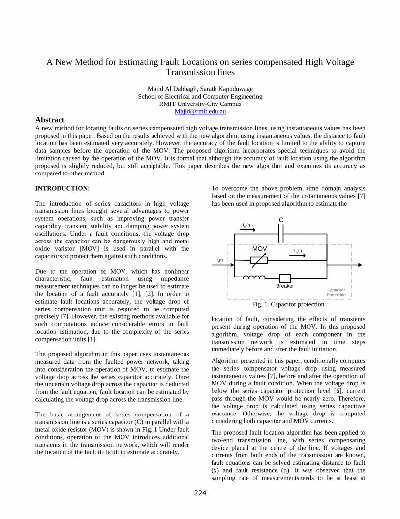
A New Method for Estimating Fault Locations on series compensated High Voltage Transmission lines
Majid Al Dabbagh, Sarath Kapuduwage
School of Electrical and Computer Engineering RMIT University-City Campus
[email protected] Abstract A new method for locating faults on series compensated high voltage transmission lines, using instantaneous values has been proposed in this paper. Based on the results achieved with the new algorithm, using instantaneous values, the distance to fault location has been estimated very accurately. However, the accuracy of the fault location is limited to the ability to capture data samples before the operation of the MOV. The proposed algorithm incorporates special techniques to avoid the limitation caused by the operation of the MOV. It is formal that although the accuracy of fault location using the algorithm proposed is slightly reduced, but still acceptable. This paper describes the new algorithm and examines its accuracy as compared to other method. INTRODUCTION: The introduction of series capacitors in high voltage transmission lines brought several advantages to power system operations, such as improving power transfer capability, transient stability and damping power system oscillations. Under a fault conditions, the voltage drop across the capacitor can be dangerously high and metal oxide varistor [MOV] is used in parallel with the capacitors to protect them against such conditions. Due to the operation of MOV, which has nonlinear characteristic, fault estimation using impedance measurement techniques can no longer be used to estimate the location of a fault accurately [1], [2]. In order to estimate fault locations accurately, the voltage drop of series compensation unit is required to be computed precisely [7]. However, the existing methods available for such computations induce considerable errors in fault location estimation, due to the complexity of the series compensation units [1]. The proposed algorithm in this paper uses instantaneous measured data from the faulted power network, taking into consideration the operation of MOV, to estimate the voltage drop across the series capacitor accurately. Once the uncertain voltage drop across the capacitor is deducted from the fault equation, fault location can be estimated by calculating the voltage drop across the transmission line. The basic arrangement of series compensation of a transmission line is a series capacitor (C) in parallel with a metal oxide resistor (MOV) is shown in Fig. 1 Under fault conditions, operation of the MOV introduces additional transients in the transmission network, which will render the location of the fault difficult to estimate accurately.
To overcome the above problem, time domain analysis based on the measurement of the instantaneous values [7] has been used in proposed algorithm to estimate the
C
MOV
BreakerCapacitorProtection
If(t)
Icp(t)
Imv(t)
Fig. 1. Capacitor protection
location of fault, considering the effects of transients present during operation of the MOV. In this proposed algorithm, voltage drop of each component in the transmission network is estimated in time steps immediately before and after the fault initiation.
Algorithm presented in this paper, conditionally computes the series compensator voltage drop using measured instantaneous values [7], before and after the operation of MOV during a fault condition. When the voltage drop is below the series capacitor protection level [6], current pass through the MOV would be nearly zero. Therefore, the voltage drop is calculated using series capacitive reactance. Otherwise, the voltage drop is computed considering both capacitor and MOV currents.
The proposed fault location algorithm has been applied to two-end transmission line, with series compensating device placed at the centre of the line. If voltages and currents from both ends of the transmission are known, fault equations can be solved estimating distance to fault (x) and fault resistance (rf). It was observed that the sampling rate of measurementsneeds to be at least at
224
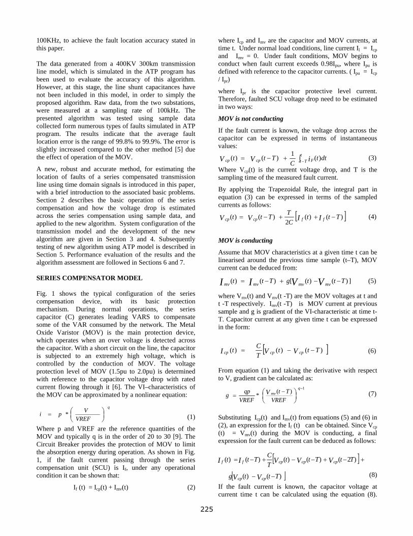
100KHz, to achieve the fault location accuracy stated in this paper. The data generated from a 400KV 300km transmission line model, which is simulated in the ATP program has been used to evaluate the accuracy of this algorithm. However, at this stage, the line shunt capacitances have not been included in this model, in order to simply the proposed algorithm. Raw data, from the two substations, were measured at a sampling rate of 100kHz. The presented algorithm was tested using sample data collected form numerous types of faults simulated in ATP program. The results indicate that the average fault location error is the range of 99.8% to 99.9%. The error is slightly increased compared to the other method [5] due the effect of operation of the MOV.
⎟⎠⎞
⎜⎝⎛=
VREFVpi
q
*
A new, robust and accurate method, for estimating the location of faults of a series compensated transmission line using time domain signals is introduced in this paper, with a brief introduction to the associated basic problems. Section 2 describes the basic operation of the series compensation and how the voltage drop is estimated across the series compensation using sample data, and applied to the new algorithm. System configuration of the transmission model and the development of the new algorithm are given in Section 3 and 4. Subsequently testing of new algorithm using ATP model is described in Section 5. Performance evaluation of the results and the algorithm assessment are followed in Sections 6 and 7. SERIES COMPENSATOR MODEL Fig. 1 shows the typical configuration of the series compensation device, with its basic protection mechanism. During normal operations, the series capacitor (C) generates leading VARS to compensate some of the VAR consumed by the network. The Metal Oxide Varistor (MOV) is the main protection device, which operates when an over voltage is detected across the capacitor. With a short circuit on the line, the capacitor is subjected to an extremely high voltage, which is controlled by the conduction of MOV. The voltage protection level of MOV (1.5pu to 2.0pu) is determined with reference to the capacitor voltage drop with rated current flowing through it [6]. The VI–characteristics of the MOV can be approximated by a nonlinear equation:
(1)
Where p and VREF are the reference quantities of the MOV and typically q is in the order of 20 to 30 [9]. The Circuit Breaker provides the protection of MOV to limit the absorption energy during operation. As shown in Fig. 1, if the fault current passing through the series compensation unit (SCU) is If, under any operational condition it can be shown that:
If (t) = Icp(t) + Imv(t) (2)
where Icp and Imv are the capacitor and MOV currents, at time t. Under normal load conditions, line current Il = Icp and Imv = 0. Under fault conditions, MOV begins to conduct when fault current exceeds 0.98Ipu, where Ipu is defined with reference to the capacitor currents. ( Ipu = Icp / Ipr)
where Ipr is the capacitor protective level current. Therefore, faulted SCU voltage drop need to be estimated in two ways:
MOV is not conducting
If the fault current is known, the voltage drop across the capacitor can be expressed in terms of instantaneous values:
(3)
Where Vcp(t) is the current voltage drop, and T is the sampling time of the measured fault current.
dttC
Ttt tTt Fcp
By applying the Trapezoidal Rule, the integral part in equation (3) can be expressed in terms of the sampled currents as follows:
(4)
MOV is conducting
Assume that MOV characteristics at a given time t can be linearised around the previous time sample (t–T), MOV current can be deduced from:
])()([)()( TttgTtt VVII mvmvmvmv −−+−= (5)
where Vmv(t) and Vmv(t -T) are the MOV voltages at t and t -T respectively. Imv(t -T) is MOV current at previous sample and g is gradient of the VI-characteristic at time t-T. Capacitor current at any given time t can be expressed in the form:
(6)
From equation (1) and taking the derivative with respect to V, gradient can be calculated as: (7)
Substituting Icp(t) and Imv(t) from equations (5) and (6) in (2), an expression for the If (t) can be obtained. Since Vcp (t) = Vmv(t) during the MOV is conducting, a final expression for the fault current can be deduced as follows:
(8)
If the fault current is known, the capacitor voltage at current time t can be calculated using the equation (8).
cpV ( −= iV )(1)() ∫ −+
[ ])()(2
)()( TttCTTV cp tt IIV ffcp −++−=
[ ])()()( TVI = ttTCt V cpcpcp −−
[ ] +−+−−+−= )2()()()()( TtTttTCTtt VVVII cpcpcpff
[ ])()( Tttg VV cpcp −−
⎟⎞qp q
⎠⎜⎝⎛ −
=−
VREFTt
VREFg V mv )(*
1
225
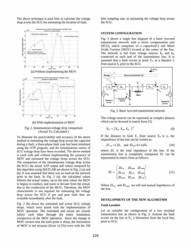
The above technique is used here to calculate the voltage drop across the SCU for estimating the location of fault.
0 10 20 30 40 50 60-4
-3
-2
-1
0
1
2
3
4x 10 5
Tim e , m s
SCU
Vol
tage
Dro
p(in
Vol
ts)
Com pa rision of SCU insta nta nious volta ge drop Acuta l V s ca lcula te d
Fau lt Incep tion
Actua l vo ltage d rop
C a lu la ted vo ltage d rop
VR & IR
FLoc.
ES
Station S(Local)
ZS ZL11 ZL22 ZR
MOV
C
ER
F2
ISIR
IF
VS VR
Station R(Remote)
Microwave/Sattelite link
F1
Distance to fault (x)
(a) Without implementing the MOV
(b) With implementation of MOV
Fig. 2. Instantaneous voltage drop comparison (Actual Vs. Calculated )
To illustrate the practicability and accuracy of the above method in estimating the voltage drop across the capacitor during a fault, a three-phase fault case has been simulated using the ATP program, and the instantaneous values of SCU voltage drop have been recorded. The above method is used with and without implementing the presence of MOV and estimated the voltage drops across the SCU. The comparison of the instantaneous voltage drop across the SCU; the actual ATP output and values computed by this algorithm using MATLAB are shown in Fig. 2 (a) and (b). It was assumed that there was no load on the network prior to the fault. In Fig. 2 (a), the calculated values follows the actual values, up to the time where the MOV is begins to conduct, and starts to deviate from the actual, due to the conduction of the MOV. Therefore, the MOV characteristic is not required for estimating the voltage drop across the SCU if pre and post fault data are available immediately after the fault.
Fig. 2 (b) shows the estimated and actual SCU voltage drops, which were tested with the implementation of MOV operation. The estimated and actual are closely follow each other through the entire simulation, irrespective of the MOV operation. Since the change in MOV current near the knee point is sharp, the linerisation of MOV is not accurate (Error ±2.5%) even with the 100
kHz sampling rate, in estimating the voltage drop across the SCU.
0 10 20 30 40 50 60-4
-3
-2
-1
0
1
2
3
4x 10⁵
SCU
Vol
tage
Dro
p(in
Vol
ts)
Com pa rision of S CU insta nta n ious volta ge drop Acuta l V s ca lcula te d
Fault Inception
M OV conduc tion s ta r ts (devia tes from ca lcula ted)
Ac tua l voltage drop
Ca lcula ted voltage drop
Tim e , m s
SYSTEM CONFIGURATION
Fig. 3 shows a single line diagram of a basic two-end transmission network with a series compensation unit (SCU), which comprises of a capacitor(C) and Metal Oxide Varistor (MOV) located at the center of the line. The network is fed from voltage sources ES and ER connected to each end of the transmission line. It is assumed that a fault occurs at point F1, at a distance x from source S, prior to the SCU.
Fig. 3. Basic two-end transmission network The voltage sources can be expressed as complex phasors which can be denoted in matrix form [3]:
ES = [ Esa Esb Esc ] T (9) If the distance to fault F1 from source ES is x, the impendence of the line can be written as:
ZL11 =x ZL and ZL22=(1-x)ZL (10)
where ZL is the total impedance of the line. If the transmission line is completely transposed ZL can be represented in matrix form as follows:
⎥⎥⎥
⎦
⎤
⎢⎢⎢
⎣
⎡=
ZLZLZLZLZLZLZLZLZL
ZL
ssmmmm
mmssmm
mmmmss
(11)
Where ZLss and ZLmm are self and mutual impedances of the line. DEVELOPMENT OF THE NEW ALGORITHM
Fault Location
Let us consider the configuration of a two terminal transmission line as shown in Fig. 3. Assume the fault occurs on the line at F1, x kilometers from the local bus, prior to SCU.
226
If the voltage and current at the local bus and remote buses are Vs, Is, VR and IR respectively, then the network equation of the faulted system can be written in matrix form:
(12)
where [VD] is the voltage drop across the series compensation unit. Using IB data samples in equation (8), the instantaneous values of [VD] can be calculated. However, the computation of current value of [VD] requires its previous value. Initial values for [VD] can be estimated applying pre fault values to the network equations.
At any given time, the instantaneous voltage drop across the impedance with inductance L and resistance R can be written in discrete form as:
(13)
Where I(t) is the current passing through the impedance at time t. Knowing IS and IR, the instantaneous values of [ZL]IS] and ,[ZL]IR] are calculated using equation (13). Solution for distance to fault x can be estimated for each instantaneous value using the following expression:
(14)
where t0 is the time at which sample values are computed. Measured voltages and computed voltage drops are 3x1 matrices for a 3-phase line and must be solved using matrix operations.
Locating Fault with respect to SCU
If the fault occurs at F2, as shown in Fig. 3 after the SCU, equation (12) needs to be adjusted as follows:
The application of correct equations for locating fawith respect to the position of SCU can be describedfollows: Since the SCU is located at the middle of ldistance to the fault x could be estimated using equa(14), and the result should be in the range of x > 0 an<= 0.5. If the value of x is not in this range, equation will correctly estimate the fault location.
Fault Resistance
A general 3-phase fault model is implemented in flocation algorithm to estimate the fault resistance [2]phase fault conduction matrix can be stated in maform:
Where Rf is the aggregated fault resistance and VF isvoltage at the fault. The fault matrix KF need tocomputed in relation to the type of fault [2]. Apply
fault equation to the opposite side of series compensation unit:
Where VF is the voltage at the fault location. If the fault type and distance to fault are known, fault resistance can be calculated using equation (16) and (17). TESTING AND EVALUATION
Transmission line Model
In order to statistically test the accuracy and robustness of the newly developed algorithm, a two terminal, 3-phase transmission model as shown in Fig. 3, was modeled using the ATP program.
The transmission line model used is 300km long and rated at 400KV. The series compensation unit is placed and fixed in the middle of the line. The supply systems are represented by mutually coupled R L branches together with ideal voltage sources [9].
The transmission line is represented by two sections of 3 -phase mutually coupled R L branches specifying positive and zero sequence impedance for each branch. The Series compensation unit consists of a capacitor and MOV and it has the v-i characteristics of ZnO surge arrester represented by a non-linear equation similar to equation (1).
The flash over voltage of the gap is specified in order to fire the gap during heavy fault currents. Voltages and currents from both ends are recorded at sampling rate of 100 KHz before and after fault occurrence. Total simulation time is 0.1 sec. and the fault is initiated at 0.035 sec.
For statistical evaluations, the same data file was modeled
[ ] [ ][ ] [ ] [ ][ ] [ ]VIVIV DRRSs ZLxZLx −−−=− )1(
[ ])()()(.)( TtItITLtIRtV −−+=
)()()()()()()(
00
00000
tVZtVZtVZtVtVtVtx
RS
RDBA
+++−
=
)()()()()()()(
00
00000
tVZtVZtVZtVtVtVtx
RR
RDBA
++−−
= )
[ ] [ ][
[ ] [ ] [ ]III
VKR
I
RSF
FFf
F
+=
=1 ]
( )[ ] [ ] [ ][ ]IVV RRF ZLx )1( −−=
(
(15
ults as
ine, tion d x
(15)
ault . 3-trix
the be ing
using the ATP program, with minor modificationscover the broad spectrum of faults. The system data ufor this model are shown in table 1.
Table 1. System data used for the transmission line
PARAMETER TRANS. LINE SYS. S AND R pos. sequence impedence (ohm) zero sequence impedence (ohm)
8.25 + j94.5 82.5 +j308
1.31 + j15.0 2.33 + j26.8
Length (kM) Voltage (kV) degree of compensation (%) location of SCU (kM) shunt capacitance (ohm)
300 400 89 150 -
MOV DATA used in ATP model reference current (kA) reference voltage (kV) exponent
4.4 330 23
sampling frequency (kHz) 100
SOURCES
)
227
17
to sed
16
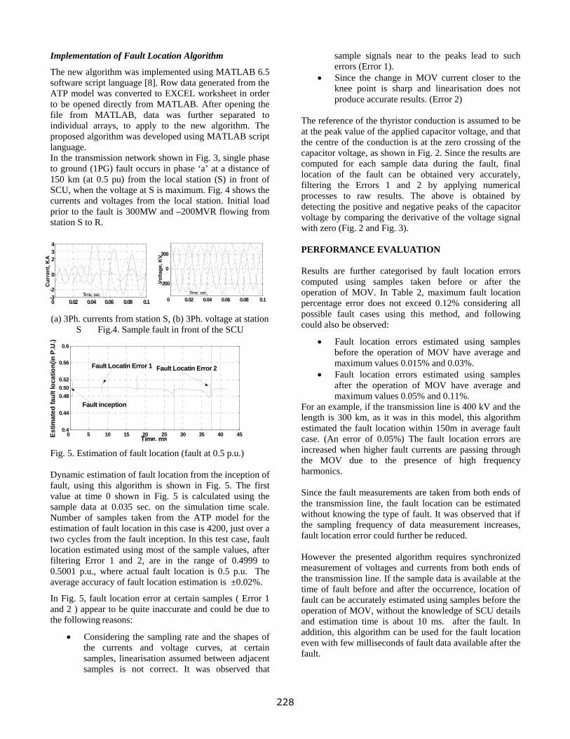
Implementation of Fault Location Algorithm
The new algorithm was implemented using MATLAB 6.5 software script language [8]. Row data generated from the ATP model was converted to EXCEL worksheet in order to be opened directly from MATLAB. After opening the file from MATLAB, data was further separated to individual arrays, to apply to the new algorithm. The proposed algorithm was developed using MATLAB script language. In the transmission network shown in Fig. 3, single phase to ground (1PG) fault occurs in phase ‘a’ at a distance of 150 km (at 0.5 pu) from the local station (S) in front of SCU, when the voltage at S is maximum. Fig. 4 shows the currents and voltages from the local station. Initial load prior to the fault is 300MW and –200MVR flowing from station S to R. (a) 3Ph. currents from station S, (b) 3Ph. voltage at station
S Fig.4. Sample fault in front of the SCU
Fig. 5. Estimation of fault location (fault at 0.5 p.u.) Dynamic estimation of fault location from the inception of fault, using this algorithm is shown in Fig. 5. The first value at time 0 shown in Fig. 5 is calculated using the sample data at 0.035 sec. on the simulation time scale. Number of samples taken from the ATP model for the estimation of fault location in this case is 4200, just over a two cycles from the fault inception. In this test case, fault location estimated using most of the sample values, after filtering Error 1 and 2, are in the range of 0.4999 to 0.5001 p.u., where actual fault location is 0.5 p.u. The average accuracy of fault location estimation is ±0.02%.
In Fig. 5, fault location error at certain samples ( Error 1 and 2 ) appear to be quite inaccurate and could be due to the following reasons:
• Considering the sampling rate and the shapes of the currents and voltage curves, at certain samples, linearisation assumed between adjacent samples is not correct. It was observed that
sample signals near to the peaks lead to such errors (Error 1).
• Since the change in MOV current closer to the knee point is sharp and linearisation does not produce accurate results. (Error 2)
The reference of the thyristor conduction is assumed to be at the peak value of the applied capacitor voltage, and that the centre of the conduction is at the zero crossing of the capacitor voltage, as shown in Fig. 2. Since the results are computed for each sample data during the fault, final location of the fault can be obtained very accurately, filtering the Errors 1 and 2 by applying numerical processes to raw results. The above is obtained by detecting the positive and negative peaks of the capacitor voltage by comparing the derivative of the voltage signal with zero (Fig. 2 and Fig. 3).
0 0.02 0.04 0.06 0.08 0.1-3-2
0
2
0 0.02 0.04 0.06 0.08 0.1
-200
0
200
Volta
ge, K
V
Time, sec.
PERFORMANCE EVALUATION Results are further categorised by fault location errors computed using samples taken before or after the operation of MOV. In Table 2, maximum fault location percentage error does not exceed 0.12% considering all possible fault cases using this method, and following could also be observed:
• Fault location errors estimated using samples before the operation of MOV have average and maximum values 0.015% and 0.03%.
• Fault location errors estimated using samples after the operation of MOV have average and maximum values 0.05% and 0.11%.
For an example, if the transmission line is 400 kV and the length is 300 km, as it was in this model, this algorithm estimated the fault location within 150m in average fault case. (An error of 0.05%) The fault location errors are increased when higher fault currents are passing through the MOV due to the presence of high frequency harmonics. Since the fault measurements are taken from both ends of the transmission line, the fault location can be estimated without knowing the type of fault. It was observed that if the sampling frequency of data measurement increases, fault location error could further be reduced. However the presented algorithm requires synchronized measurement of voltages and currents from both ends of the transmission line. If the sample data is available at the time of fault before and after the occurrence, location of fault can be accurately estimated using samples before the operation of MOV, without the knowledge of SCU details and estimation time is about 10 ms. after the fault. In addition, this algorithm can be used for the fault location even with few milliseconds of fault data available after the fault.
34
Cur
rent
, KA
Time, sec.
0 5 10 15 20 25 30 35 40 450.4
0.44
0.48
0.52
0.56
0.6
Time, msEstim
ated
faul
t loc
atio
n(in
P.U
.)
Fault Locatin Error 1 Fault Locatin Error 2
0.50
Fault inception
228
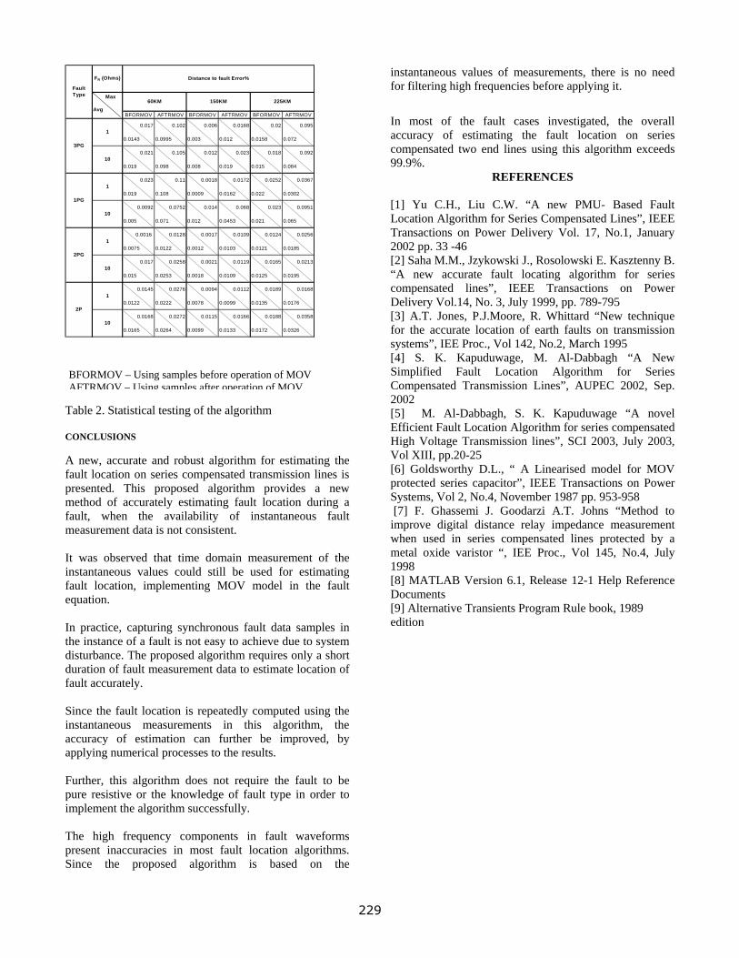
T C Afpmfm Iinfe Ithddf Sinaa Fpim TpS
instantaneous values of measurements, there is no need for filtering high frequencies before applying it.
BFORMOV AFTRMOV BFORMOV AFTRMOV BFORMOV AFTRMOV
0.017 0.102 0.006 0.0168 0.02 0.095
0.0143 0.0995 0.003 0.012 0.0158 0.072
0.021 0.105 0.012 0.023 0.018 0.092
0.019 0.098 0.008 0.019 0.015 0.084
0.023 0.11 0.0018 0.0172 0.0252 0.0367
0.019 0.108 0.0009 0.0162 0.022 0.0302
0.0092 0.0752 0.014 0.068 0.023 0.0951
0.005 0.071 0.012 0.0453 0.021 0.065
0.0016 0.0128 0.0017 0.0109 0.0124 0.0256
0.0075 0.0122 0.0012 0.0103 0.0121 0.0185
0.017 0.0258 0.0021 0.0119 0.0165 0.0213
0.015 0.0253 0.0018 0.0109 0.0125 0.0195
0.0145 0.0276 0.0094 0.0112 0.0189 0.0168
0.0122 0.0222 0.0078 0.0099 0.0135 0.0176
0.0168 0.0272 0.0115 0.0166 0.0188 0.0358
0.0165 0.0264 0.0099 0.0133 0.0172 0.0326
1
1
10
1PG
2PG
2P
10
1
10
Distance to fault Error%FR (Ohms)
Fault Type
3PG
150KM 225KM60KM
1
10
Max
Avg In most of the fault cases investigated, the overall accuracy of estimating the fault location on series compensated two end lines using this algorithm exceeds 99.9%.
REFERENCES
[1] Yu C.H., Liu C.W. “A new PMU- Based Fault Location Algorithm for Series Compensated Lines”, IEEE Transactions on Power Delivery Vol. 17, No.1, January 2002 pp. 33 -46 [2] Saha M.M., Jzykowski J., Rosolowski E. Kasztenny B. “A new accurate fault locating algorithm for series compensated lines”, IEEE Transactions on Power Delivery Vol.14, No. 3, July 1999, pp. 789-795 [3] A.T. Jones, P.J.Moore, R. Whittard “New technique for the accurate location of earth faults on transmission systems”, IEE Proc., Vol 142, No.2, March 1995 [4] S. K. Kapuduwage, M. Al-Dabbagh “A New Simplified Fault Location Algorithm for Series Compensated Transmission Lines”, AUPEC 2002, Sep.
BA
FORMOV – Using samples before operation of MOV FTRMOV – Using samples after operation of MOV
able 2. Statistical testing of the algorithm
ONCLUSIONS
new, accurate and robust algorithm for estimating the ault location on series compensated transmission lines is resented. This proposed algorithm provides a new ethod of accurately estimating fault location during a
ault, when the availability of instantaneous fault easurement data is not consistent.
t was observed that time domain measurement of the stantaneous values could still be used for estimating
ault location, implementing MOV model in the fault quation.
n practice, capturing synchronous fault data samples in e instance of a fault is not easy to achieve due to system
isturbance. The proposed algorithm requires only a short uration of fault measurement data to estimate location of ault accurately.
ince the fault location is repeatedly computed using the stantaneous measurements in this algorithm, the
ccuracy of estimation can further be improved, by pplying numerical processes to the results.
urther, this algorithm does not require the fault to be ure resistive or the knowledge of fault type in order to
plement the algorithm successfully.
he high frequency components in fault waveforms resent inaccuracies in most fault location algorithms. ince the proposed algorithm is based on the
2002 [5] M. Al-Dabbagh, S. K. Kapuduwage “A novel Efficient Fault Location Algorithm for series compensated High Voltage Transmission lines”, SCI 2003, July 2003, Vol XIII, pp.20-25 [6] Goldsworthy D.L., “ A Linearised model for MOV protected series capacitor”, IEEE Transactions on Power Systems, Vol 2, No.4, November 1987 pp. 953-958 [7] F. Ghassemi J. Goodarzi A.T. Johns “Method to improve digital distance relay impedance measurement when used in series compensated lines protected by a metal oxide varistor “, IEE Proc., Vol 145, No.4, July 1998 [8] MATLAB Version 6.1, Release 12-1 Help Reference Documents [9] Alternative Transients Program Rule book, 1989 edition
229
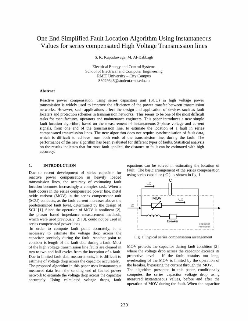
One End Simplified Fault Location Algorithm Using Instantaneous Values for series compensated High Voltage Transmission lines
S. K. Kapuduwage, M. Al-Dabbagh
Electrical Energy and Control Systems
School of Electrical and Computer Engineering RMIT University – City Campus [email protected]
Abstract Reactive power compensation, using series capacitors unit (SCU) in high voltage power transmission is widely used to improve the efficiency of the power transfer between transmission networks. However, such applications affect the design and application of devices such as fault locaters and protection schemes in transmission networks. This seems to be one of the most difficult tasks for manufactures, operators and maintenance engineers. This paper introduces a new simple fault location algorithm, based on the measurement of instantaneous 3-phase voltage and current signals, from one end of the transmission line, to estimate the location of a fault in series compensated transmission lines. The new algorithm does not require synchronisation of fault data, which is difficult to achieve from both ends of the transmission line, during the fault. The performance of the new algorithm has been evaluated for different types of faults. Statistical analysis on the results indicates that for most fault applied, the distance to fault can be estimated with high accuracy.
1. INTRODUCTION
Due to recent development of series capacitor for reactive power compensation in heavily loaded transmission lines, the accuracy of estimating fault location becomes increasingly a complex task. When a fault occurs in the series compensated power line, metal oxide varistor (MOV) in the series compensator unit (SCU) conducts, as the fault current increases above the predetermined fault level, determined by the design of SCU [1]. Since the operation of MOV is nonlinear [2], the phasor based impedance measurement methods, which were used previously [2] [3], could not be used in series compensated power lines. In order to compute fault point accurately, it is necessary to estimate the voltage drop across the capacitor precisely during the fault. Another point to consider is length of the fault data during a fault. Most of the high voltage transmission line faults are cleared in two to two and half cycles from the inception of a fault. Due to limited fault data measurements, it is difficult to estimate of voltage drop across the capacitor accurately. The proposed algorithm in this paper uses instantaneous measured data from the sending end of faulted power network to estimate the voltage drop across the capacitor accurately. Using calculated voltage drops, fault
equations can be solved in estimating the location of fault. The basic arrangement of the series compensation using series capacitor ( C ) is shown in fig. 1.
C
MOV
BreakerCapacitorProtection
If(t)
Icp(t)
Imv(t)
Fig. 1 Typical series compensation arrangement
MOV protects the capacitor during fault condition [2], where the voltage drop across the capacitor exceeds its protective level. If the fault sustains too long, overheating of the MOV is limited by the operation of the breaker, bypassing the current through the MOV. The algorithm presented in this paper, conditionally computes the series capacitor voltage drop using measured instantaneous values, before and after the operation of MOV during the fault. When the capacitor
230
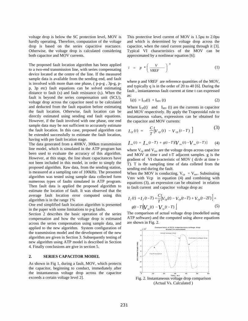
⎟⎠⎞
⎜⎝⎛=
VREFVpi
q
*
0 1 0 2 0 3 0 4 0 5 0 6 0-4
-3
-2
-1
0
1
2
3
4x 1 0 5
T i
voltage drop is below the SC protection level, MOV is hardly operating. Therefore, computation of the voltage drop is based on the series capacitive reactance. Otherwise, the voltage drop is calculated considering both capacitor and MOV currents. The proposed fault location algorithm has been applied to a two-end transmission line, with series compensating device located at the centre of the line. If the measured sample data is available from the sending end, and fault is involved with more than one phase, ( p-p-g , 3p-g, p-p, 3p etc) fault equations can be solved estimating distance to fault (x) and fault resistance (rf). When the fault is beyond the series compensation unit (SCU), voltage drop across the capacitor need to be calculated and deducted from the fault equation before estimating the fault location. Otherwise, fault location can be directly estimated using sending end fault equations. However, if the fault involved with one phase, one end sample data may be not sufficient to accurately estimate the fault location. In this case, preposed algorithm can be extended successfully to estimate the fault location, having with pre fault location stage.
m e , m s
SCU
Vol
tage
Dro
p(in
Vol
ts)
Co m p a risio n o f S C U in sta n ta n io u s vo lta g e d ro p A cu ta l V s ca lcu la te d
Fa u lt In ce p tio n
Actu a l vo lta g e d ro p
C a lu la te d vo lta g e d ro p
The data generated from a 400KV, 300km transmission line model, which is simulated in the ATP program has been used to evaluate the accuracy of this algorithm. However, at this stage, the line shunt capacitances have not been included in this model, in order to simply the proposed algorithm. Raw data, from the sending station, is measured at a sampling rate of 100kHz. The presented algorithm was tested using sample data collected form numerous types of faults simulated in ATP program. Then fault data is applied the proposed algorithm to estimate the location of fault. It was observed that the average fault location error computed using this algorithm is in the range 1% One end simplified fault location algorithm is presented in the paper with some limitations to p-g faults. Section 2 describes the basic operation of the series compensation and how the voltage drop is estimated across the series compensation using sample data, and applied to the new algorithm. System configuration of the transmission model and the development of the new algorithm are given in Section 3. Subsequently testing of new algorithm using ATP model is described in Section 4. Finally conclusions are give in section 5. 2. SERIES CAPACITOR MODEL
As shown in Fig 1, during a fault, MOV, which protects the capacitor, beginning to conduct, immediately after the instantaneous voltage drop across the capacitor exceeds a certain voltage level 2].
This protective level current of MOV is 1.5pu to 2.0pu and which is determined by voltage drop across the capacitor, when the rated current passing through it [3]. Typical VI characteristics of the MOV can be approximated by a nonlinear equation [6]:
(1)
where p and VREF are reference quantities of the MOV, and typically q is in the order of 20 to 40 [6]. During the fault , instantaneous fault current at time t can expressed as: If(t) = ICP(t) + IMV (t) (2)
Where ICP(t) and IMV (t) are the currents in capacitor and MOV respectively. By apply the Trapezoidal rule to instantaneous values, expressions can be obtained for the capacitor and MOV currents:
(3) [ ])()()( TttTCt VVI cpcpcp −−=
])()()[()()( TttTtgTtt VVII mvmvmvmv −−−+−= (4)
where Vcp and Vmv are the voltage drops across capacitor and MOV at time t and t-T adjacent samples. g is the gradient of VI characteristic of MOV ( di/dv at time t-T). T is the sampling time of data colleted from the sending end during the fault. When the MOV is conducting, Vcp = Vmv. Substituting Vmv with Vcp in equation (4) and combining with equations (3), an expression can be obtained in relation to fault current and capacitor voltage drop as:
(5)
[ ] +−+−−+−= )2()()()()( TtTttTCTtt VVVII cpcpcpff
The comparison of actual voltage drop (modelled using ATP software) and the computed using above equations are shown in Fig. 2.
[ ])()()( TttTtg VV cpcp−−−
Fig. 2. Instantaneous voltage drop comparison (Actual Vs. Calculated )
231

The estimated and actual are closely follow each other through the entire simulation, irrespective of the MOV operation. Since the change in MOV current near the knee point is sharp, the linearization of MOV is not accurate (Error ±2.5%) even with the 100 kHz sampling rate, in estimating the voltage drop across the SCU [4]. 3. THE NEW FAULT LOCATION ALGORITHM 3.1 Transmission Line Model
The new algorithm is developed for a single 3-phase two ends transmission power network with SCU in the middle of the line. as shown in Fig 3.
Fig. 3 Simplified two-end transmission network The voltage sources can be expressed as complex phasors, which can be denoted in matrix form [3]: ES = [ Esa Esb Esc ] T (6) If the distance to fault F1 from source ES is x, the impendence of the line can be written as: ZL11 = x ZL and ZL22 = (1-x) ZL (7) where ZL is the total impedance of the line. If the transmission line is completely transposed ZL can be represented in matrix form as follows:
(8) Where ZLss and ZLmm are self and mutual impedances of the line. 3.2 Algorithm Development
Let us consider a two phase to ground fault in a two port network, and fault is occurred after the SCU, at distance x from the sending end. If the faulted point voltage is VG, fault equation can written to the sending end of the transmission network:
[ ] [ ] [ ] [ ] [ ]VVIV GDSs
ZLx =−− (9) Where VS is the sending end voltage and IS is the sending end fault current. VG and VD are voltages at fault point and SCU voltage drop respectively. Using phases a, b and c, equation 8 can be expanded as
(10) where s and m are subscripts of Z, refer to the self and mutual impedances of the transmission line. For two phase to ground fault (a-b-g), voltages at the fault point in phase A and B are nearly equal. Therefore, equation 10 can be rearranged to obtain the expression for the fault location:
(11) For completely transposed transmission lines mutual impedances are nearly equal. Therefore, equation 11 can be simplified and rewrite as:
(12) Since sending end fault currents ( ISA, ISB ) and voltages(VSA, VSB) are measured and sample values are known, fault point can be estimated using time domain analysis. First compute the SCU voltage drop ( VDA & VDB ) as explained in section 2. Lower part of equation consists of tow parts and can be computed using differential equation ( R*i + L *di/dt) [4]. Finally, value for x can be computed in time domain using equation (12). If value of x at time t is x (t):
(13) where VZISA(t) and VZISB(t) are the instantaneous voltage drops equivalent to denominator of equation (12) calculated at time t. 3.3 Fault Point with respect to SCU
The algorithm described up to now, assuming fault is occurred behind the SCU. If the fault is in front of SCU, fault equation does not contain the SCU voltage drop. Therefore, fault location estimation is easer than the previous case. Following approach could be adopted to find the selection of fault point. First compute the fault
⎥⎥⎥
⎦
⎤
⎢⎢⎢
⎣
⎡
=⎥⎥⎥
⎦
⎤
⎢⎢⎢
⎣
⎡
−⎥⎥⎥
⎦
⎤
⎢⎢⎢
⎣
⎡
⎥⎥⎥
⎦
⎤
⎢⎢⎢
⎣
⎡
−⎥⎥⎥
⎦
⎤
⎢⎢
VVV
VVV
III
ZZZZZZZZZ
VVV
GC
GB
GA
DC
DB
DA
SC
SB
SA
SCCMCBMCA
MBCSBBMBA
MACMABSAA
SC
SB
SA
x⎢⎡
⎣
(1-x)ZL
MOV
C
VF
F2
IF
F1
Station R
ES
Station S
ZS xZL
IS
VS FL
ZR
ER
IR
VR
( ) ( ) ( )IZZIZZIZZVVVV
SCMACMBCSBMBASBBSAMBASAA
DBDASBSAx−−−
+++
−−=
)( ) ( IZZIZZVVVV
SBMBASBBSAMBASAA
DBDASBSAx−−
++
−−=
⎥⎥⎥
⎦
⎤
⎢⎢⎢
⎣
⎡
=
ZLZLZLZLZLZLZLZLZL
ssmmmm
mmssmm
mmmmss
ZL)()(
)()()()()(
tVZISBtVZISA
tttttx
VVVV DBDASBSA
+
−−=
+
232
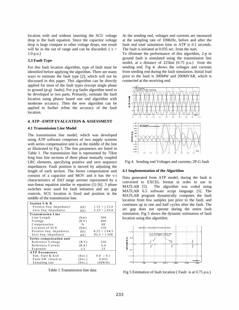
location with and without inserting the SCU voltage drop to the fault equation. Since the capacitor voltage drop is large compare to other voltage drops, one result will be in the out of range and can be discarded. ( x > 1.0 p.u.)
3.3 Fault Type
For this fault location algorithm, type of fault must be identified before applying the algorithm. There are many ways to estimate the fault type [2], which will not be discussed in this paper. This algorithm can be directly applied for most of the fault types (except single phase to ground (p-g) faults). For p-g faults algorithm need to be developed in two parts. Primarily, estimate the fault location using phasor based one end algorithm with moderate accuracy. Then the new algorithm can be applied to further refine the accuracy of the fault location. 4. ATP –EMTP EVALUATION & ASSESSMENT
4.1 Transmission Line Model
The transmission line model, which was developed using ATP software comprises of two supply systems with series compensation unit is at the middle of the line as illustrated in Fig 3. The line parameters are listed in Table 1. The transmission line is represented by 75km long four line sections of three phase mutually coupled LRC elements, specifying positive and zero sequence impedances. Fault position is moved by adjusting the length of each section. The Series compensation unit consists of a capacitor and MOV and it has the v-i characteristics of ZnO surge arrester represented by a non-linear equation similar to equation (1) [6]. 3 phase switches were used for fault initiation and arc gap controls. SCU location is fixed and position in the middle of the transmission line.
Table 1 Transmission line data
At the sending end, voltages and currents are measured at the sampling rate of 100KHz, before and after the fault and total simulation time in ATP is 0.1 seconds. The fault is initiated at 0.035 sec. from the start. To illustrate the performance of this algorithm, 2-p to ground fault is simulated using the transmission line model, at a distance of 225km (0.75 p.u.) from the sending end. Fig 4. shows the voltages and currents from sending end during the fault simulation. Initial load prior to the fault is 300MW and 200MVAR, which is connected at the receiving end.
Fig 4. Sending end Voltages and currents; 2P-G fault 4.1 Implementation of the Algorithm
Data generated from ATP model, during the fault is converted to EXCEL format in order to use in MATLAB [5]. The algorithm was coded using MATLAB 6.5 software script language [5]. The MATLAB program dynamically computes the fault location from few samples just prior to the fault, and continues up to one and half cycles after the fault. The arc gap does not operate during the entire fault simulation. Fig 5 shows the dynamic estimation of fault location using this algorithm.
S ta tio n S & R P o s itiv e S e q . Im p e d a n c e Z e ro S e q . Im p e d a n c e
(Ω ) (Ω )
1 .3 1 + j 1 5 .0 2 .3 3 + j 2 6 .8
T r a n s m iss io n L in e L in e L e n g th V o lta g e C o m p e n sa tio n L o c a tio n o f S C U P o sitiv e S e q . Im p e d a n c e Z e ro S e q . Im p e d a n c e
(k m ) (K V )
% (k m ) (Ω ) (Ω )
3 0 0 4 0 0 8 0
1 5 0 8 .2 5 + J 9 4 .5 8 2 .5 + J 3 0 8
S e r ie s c o m p e n sa tio n u n it R e fe re n c e V o lta g e R e fe re n c e C u rre n t E x p o n e n t
(K V ) (K A )
(-)
3 3 0 4 .4 2 3
A T P P a r a m e te r s S im . S ta r t & E n d F a u lt S W c lo se d a t S a m p lin g ra te
(S e c .) (S e c .) (S e c .)
0 .0 – 0 .1
0 .0 3 5 1 0 0 K H z
Fig 5 Estimation of fault location ( Fault is at 0.75 p.u.)
233
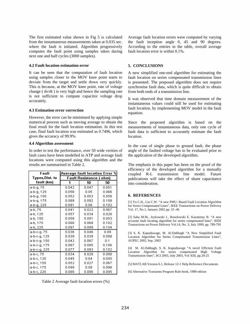
The first estimated value shown in Fig 5 is calculated from the instantaneous measurements taken at 0.035 sec. where the fault is initiated. Algorithm progressively computes the fault point using samples taken during next one and half cycles (3000 samples). 4.2 Fault location estimation error
It can be seen that the computation of fault location using samples closer to the MOV knee point starts to deviate from the target and settle down very quickly. This is because, at the MOV knee point, rate of voltage change ( dv/dt ) is very high and hence the sampling rate is not sufficient to compute capacitor voltage drop accurately. 4.3 Estimation error correction
However, the error can be minimised by applying simple numerical process such as moving average to obtain the final result for the fault location estimation. In this test case, final fault location was estimated as 0.7496, which gives the accuracy of 99.9%.
4.4 Algorithm assessment
In order to test the performance, over 50 wide verities of fault cases have been modelled in ATP and average fault locations were computed using this algorithm and the results are summarised in Table 2.
Table 2 Average fault location errors (%)
Average fault location errors were computed by varying the fault inception angle 0, 45 and 90 degrees. According to the entries in the table, overall average fault location error is within 0.1%.
5. CONCLUSIONS
A new simplified one-end algorithm for estimating the fault location on series compensated transmission lines is presented. The preposed algorithm does not require synchronise fault data, which is quite difficult to obtain from both ends of a transmission line.
It was observed that time domain measurement of the instantaneous values could still be used for estimating fault location, by implementing MOV model in the fault equation. Since the proposed algorithm is based on the measurements of instantaneous data, only one cycle of fault data is sufficient to accurately estimate the fault location. In the case of single phase to ground fault, the phase angle of the faulted voltage has to be evaluated prior to the application of the developed algorithm. The emphasis in this paper has been on the proof of the efficiency of the developed algorithm for a mutually coupled R-L transmission line model. Future publications will take the effect of shunt capacitance into consideration.
6. REFERENCES [1] Yu C.H., Liu C.W. “A new PMU- Based Fault Location Algorithm for Series Compensated Lines”, IEEE Transactions on Power Delivery Vol. 17, No.1, January 2002 pp. 33 -46 [2] Saha M.M., Jzykowski J., Rosolowski E. Kasztenny B. “A new accurate fault locating algorithm for series compensated lines”, IEEE Transactions on Power Delivery Vol.14, No. 3, July 1999, pp. 789-795 [3] S. K. Kapuduwage, M. Al-Dabbagh “A New Simplified Fault Location Algorithm for Series Compensated Transmission Lines”, AUPEC 2002, Sep. 2002 [4] M. Al-Dabbagh, S. K. Kapuduwage “A novel Efficient Fault Location Algorithm for series compensated High Voltage Transmission lines”, SCI 2003, July 2003, Vol XIII, pp.20-25 [5] MATLAB Version 6.1, Release 12-1 Help Reference Documents [6] Alternative Transients Program Rule book, 1989 edition
234

Influence of Inserting FACTS Series Capacitor on High Voltage Transmission Line on Estimation of Fault Location
ABSTRACT
Based on the developed algorithm for accurefficient fault location estimation of compensated transmission lines, the compensation unit (SCU) is assumed fixed at thof transmission line, and the fault location esusing instantaneous 3-phase voltage and signals monitored at the transmission line endpaper investigates the problems and solutions to the practical issues concerning fault destimation on transmission lines including tcontrolled switched capacitor (TCSC) with operation modes. It also investigates the osampling of data measurement required for estfault locations accurately. The effecimplementation of the proposed improvemenbeen tested using the ATP on two ends 400KVlong transmission line model. The initial indicate that the proposed developments slightthe accuracy of fault location estimation. 1. INTRODUCTION The development of power electronics applicapower systems provides great benefits in techeconomical terms. Applying FACTS compensators is one of the electronics controlenhanced power transfer capability, transient and damping of power transfer through translines. However, one of the difficulties of FACTS compensation is that the calculacapacitor voltage drop can not be estimateconvectional methods [2] [4]. The operation of FACTS devices introduces haand non linearities to the power system,adversely affect the protection systems and the
Elect
Sc
RMIT
Elec
S
R
S302
Electrical
Schoo
RMIT Uni elen
M. Al-Dabbagh rical Energy and Control
Systems hool of Electrical and
Computer Engineering
University – City Campus [email protected]
S. K. Kapuduwage trical Energy and Control
Systems chool of Electrical and
Computer Engineering MIT University – City
Campus [email protected]
ate and series series
e centre timated current s. This regards istance
hyristor various ptimum imating ts on ts have , 300km
results ly affect
tions in nical or
series lers that stability mission having
tion of d using
rmonics which fault
detection methods. To deal method of estimating fault compensated transmission lfault data, has been proposedpaper examines the applicatiFACTS series compensated practical issues related to esti The Series compensator undparts, i.e. thyristor contro(TCSC) and the protection sDuring the condition of nthyristor branch is triggeredangle and hence the voltagcapacitor can be estimated current through the TCSC [8the TCSC operates with ittherefore, accurate estimationfar more complicated, compaThis paper examines threeTCSR during light and heavynetwork to accurately estimafor all operation modes. The two ends single tranmodelled using the ATP procomputation of TCSC voltagconditions. Fig. 1: TCSC Basic Model
235
E.M. Yap Energy and Computer Engineering l of Electrical and Computer
Engineering versity – City [email protected]
with this problem, a new location for basic series
ines, using instantaneous by the authors [6]. This on of the algorithms with transmission lines and the mation of fault location.
er FACTS has two main lled switched capacitor ystem as shown in Fig. 1. ormal power operations by its pre-known firing e drop across the series using instantaneous fault
]. However, during a fault, s protection devices and of TCSC voltage drop is red to the present method.
operation modes of the faults in the transmission te the TCSC voltage drop,
smission line has been gram in order to test the e drop under various fault
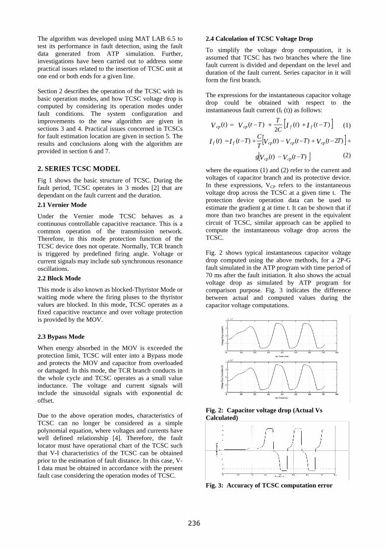
The algorithm was developed using MAT LAB 6.5 to test its performance in fault detection, using the fault data generated from ATP simulation. Further, investigations have been carried out to address some practical issues related to the insertion of TCSC unit at one end or both ends for a given line. Section 2 describes the operation of the TCSC with its basic operation modes, and how TCSC voltage drop is computed by considering its operation modes under fault conditions. The system configuration and improvements to the new algorithm are given in sections 3 and 4. Practical issues concerned in TCSCs for fault estimation location are given in section 5. The results and conclusions along with the algorithm are provided in section 6 and 7. 2. SERIES TCSC MODEL Fig 1 shows the basic structure of TCSC. During the fault period, TCSC operates in 3 modes [2] that are dependant on the fault current and the duration. 2.1 Vernier Mode
Under the Vernier mode TCSC behaves as a continuous controllable capacitive reactance. This is a common operation of the transmission network. Therefore, in this mode protection function of the TCSC device does not operate. Normally, TCR branch is triggered by predefined firing angle. Voltage or current signals may include sub synchronous resonance oscillations. 2.2 Block Mode
This mode is also known as blocked-Thyristor Mode or waiting mode where the firing pluses to the thyristor values are blocked. In this mode, TCSC operates as a fixed capacitive reactance and over voltage protection is provided by the MOV. 2.3 Bypass Mode
When energy absorbed in the MOV is exceeded the protection limit, TCSC will enter into a Bypass mode and protects the MOV and capacitor from overloaded or damaged. In this mode, the TCR branch conducts in the whole cycle and TCSC operates as a small value inductance. The voltage and current signals will include the sinusoidal signals with exponential dc offset. Due to the above operation modes, characteristics of TCSC can no longer be considered as a simple polynomial equation, where voltages and currents have well defined relationship [4]. Therefore, the fault locator must have operational chart of the TCSC such that V-I characteristics of the TCSC can be obtained prior to the estimation of fault distance. In this case, V-I data must be obtained in accordance with the present fault case considering the operation modes of TCSC.
2.4 Calculation of TCSC Voltage Drop
To simplify the voltage drop computation, it is assumed that TCSC has two branches where the line fault current is divided and dependant on the level and duration of the fault current. Series capacitor in it will form the first branch. The expressions for the instantaneous capacitor voltage drop could be obtained with respect to the instantaneous fault current (If (t)) as follows:
(1) [ ])()(2
)()( TttCTTtt IIVV ffcpcp −++−=
[ ] +−+−−+−= )2()()()()( TtTtt
TCTtt VVVII cpcpcpff
[ ])()( Tttg VV cpcp −− (2)
where the equations (1) and (2) refer to the current and voltages of capacitor branch and its protective device. In these expressions, VCP refers to the instantaneous voltage drop across the TCSC at a given time t. The protection device operation data can be used to estimate the gradient g at time t. It can be shown that if more than two branches are present in the equivalent circuit of TCSC, similar approach can be applied to compute the instantaneous voltage drop across the TCSC. Fig. 2 shows typical instantaneous capacitor voltage drop computed using the above methods, for a 2P-G fault simulated in the ATP program with time period of 70 ms after the fault initiation. It also shows the actual voltage drop as simulated by ATP program for comparison purpose. Fig. 3 indicates the difference between actual and computed values during the capacitor voltage computations. Fig. 2: Capacitor voltage drop (Actual Vs Calculated) Fig. 3: Accuracy of TCSC computation error
236
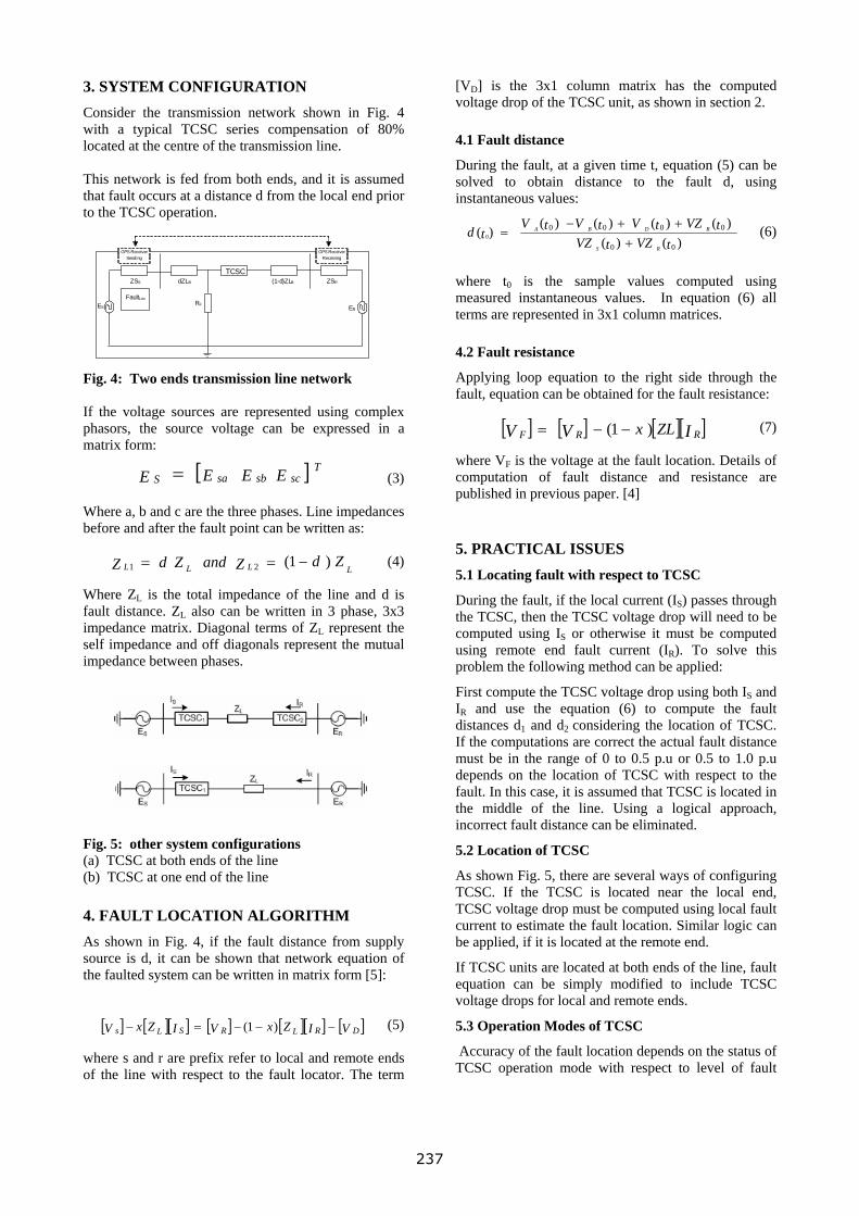
3. SYSTEM CONFIGURATION Consider the transmission network shown in Fig. 4 with a typical TCSC series compensation of 80% located at the centre of the transmission line. This network is fed from both ends, and it is assumed that fault occurs at a distance d from the local end prior to the TCSC operation. Fig. 4: Two ends transmission line network If the voltage sources are represented using complex phasors, the source voltage can be expressed in a matrix form:
(3) Where a, b and c are the three phases. Line impedances before and after the fault point can be written as:
(4) Where ZL is the total impedance of the line and d is fault distance. ZL also can be written in 3 phase, 3x3 impedance matrix. Diagonal terms of ZL represent the self impedance and off diagonals represent the mutual impedance between phases. Fig. 5: other system configurations (a) TCSC at both ends of the line (b) TCSC at one end of the line 4. FAULT LOCATION ALGORITHM As shown in Fig. 4, if the fault distance from supply source is d, it can be shown that network equation of the faulted system can be written in matrix form [5]:
(5) where s and r are prefix refer to local and remote ends of the line with respect to the fault locator. The term
[VD] is the 3x1 column matrix has the computed voltage drop of the TCSC unit, as shown in section 2. 4.1 Fault distance
During the fault, at a given time t, equation (5) can be solved to obtain distance to the fault d, using instantaneous values:
)()()()()()(
)(00
00000
tVZtVZtVZtVtVtV
tdRS
RDBA
+++−
= (6)
RF
TCSCdZLBZSS
ERES
(1-d)ZLB ZSR
FaultLoc
GPS ReceiverSending
GPS ReceiverReceiving
where t0 is the sample values computed using measured instantaneous values. In equation (6) all terms are represented in 3x1 column matrices. 4.2 Fault resistance
Applying loop equation to the right side through the fault, equation can be obtained for the fault resistance:
[ ] [ ] [ ] IVV RRF ZLx )1( − (7) [ ]−= where VF is the voltage at the fault location. Details of computation of fault distance and resistance are published in previous paper. [4]
[ ]EEEE scsbsaT
S =
5. PRACTICAL ISSUES
ZdZandZdZ LLLL )1(21 −==5.1 Locating fault with respect to TCSC
During the fault, if the local current (IS) passes through the TCSC, then the TCSC voltage drop will need to be computed using IS or otherwise it must be computed using remote end fault current (IR). To solve this problem the following method can be applied:
First compute the TCSC voltage drop using both IS and IR and use the equation (6) to compute the fault distances d1 and d2 considering the location of TCSC. If the computations are correct the actual fault distance must be in the range of 0 to 0.5 p.u or 0.5 to 1.0 p.u depends on the location of TCSC with respect to the fault. In this case, it is assumed that TCSC is located in the middle of the line. Using a logical approach, incorrect fault distance can be eliminated.
5.2 Location of TCSC
As shown Fig. 5, there are several ways of configuring TCSC. If the TCSC is located near the local end, TCSC voltage drop must be computed using local fault current to estimate the fault location. Similar logic can be applied, if it is located at the remote end.
If TCSC units are located at both ends of the line, fault equation can be simply modified to include TCSC voltage drops for local and remote ends.
][ ] [ ][ ] [ ] [ ][ ] [VIZxVIZxV DRLRSLs −−−=− )1( 5.3 Operation Modes of TCSC
Accuracy of the fault location depends on the status of TCSC operation mode with respect to level of fault
237
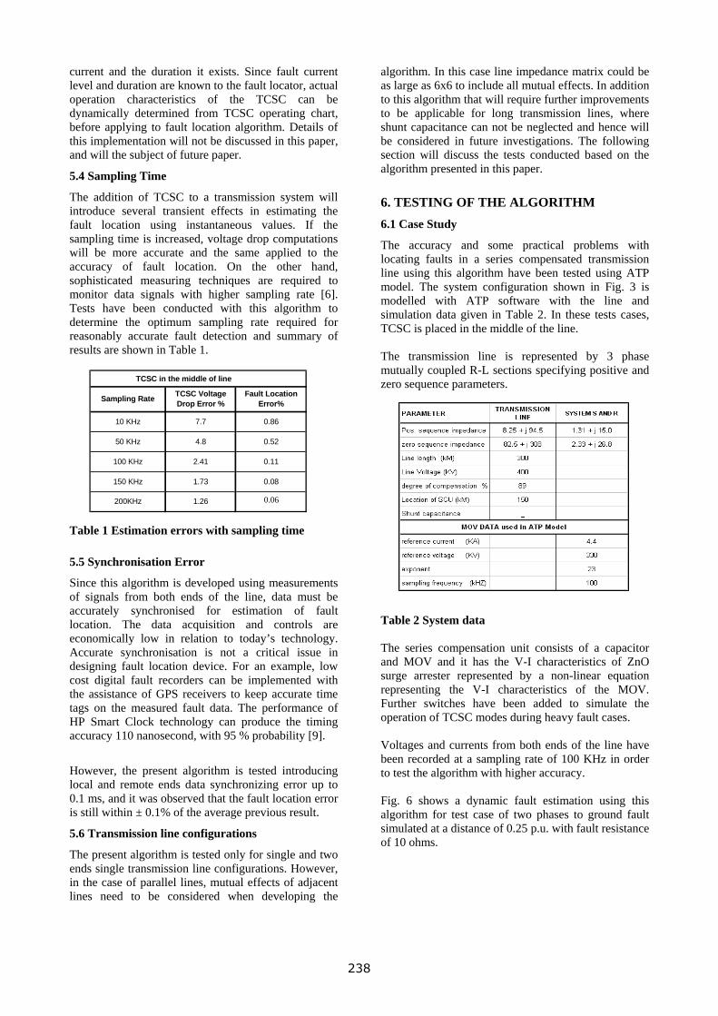
current and the duration it exists. Since fault current level and duration are known to the fault locator, actual operation characteristics of the TCSC can be dynamically determined from TCSC operating chart, before applying to fault location algorithm. Details of this implementation will not be discussed in this paper, and will the subject of future paper.
5.4 Sampling Time
The addition of TCSC to a transmission system will introduce several transient effects in estimating the fault location using instantaneous values. If the sampling time is increased, voltage drop computations will be more accurate and the same applied to the accuracy of fault location. On the other hand, sophisticated measuring techniques are required to monitor data signals with higher sampling rate [6]. Tests have been conducted with this algorithm to determine the optimum sampling rate required for reasonably accurate fault detection and summary of results are shown in Table 1. Table 1 Estimation errors with sampling time 5.5 Synchronisation Error
Since this algorithm is developed using measurements of signals from both ends of the line, data must be accurately synchronised for estimation of fault location. The data acquisition and controls are economically low in relation to today’s technology. Accurate synchronisation is not a critical issue in designing fault location device. For an example, low cost digital fault recorders can be implemented with the assistance of GPS receivers to keep accurate time tags on the measured fault data. The performance of HP Smart Clock technology can produce the timing accuracy 110 nanosecond, with 95 % probability [9].
However, the present algorithm is tested introducing local and remote ends data synchronizing error up to 0.1 ms, and it was observed that the fault location error is still within ± 0.1% of the average previous result.
5.6 Transmission line configurations
The present algorithm is tested only for single and two ends single transmission line configurations. However, in the case of parallel lines, mutual effects of adjacent lines need to be considered when developing the
algorithm. In this case line impedance matrix could be as large as 6x6 to include all mutual effects. In addition to this algorithm that will require further improvements to be applicable for long transmission lines, where shunt capacitance can not be neglected and hence will be considered in future investigations. The following section will discuss the tests conducted based on the algorithm presented in this paper.
6. TESTING OF THE ALGORITHM 6.1 Case Study
The accuracy and some practical problems with locating faults in a series compensated transmission line using this algorithm have been tested using ATP model. The system configuration shown in Fig. 3 is modelled with ATP software with the line and simulation data given in Table 2. In these tests cases, TCSC is placed in the middle of the line. The transmission line is represented by 3 phase mutually coupled R-L sections specifying positive and zero sequence parameters. TCSC in the middle of line
150 KHz 1.73 0.08
200KHz 1.26 0.61
50 KHz 4.8 0.52
100 KHz 2.41 0.11
Sampling Rate TCSC Voltage Drop Error %
Fault Location Error%
10 KHz 7.7 0.86
0.06
Table 2 System data The series compensation unit consists of a capacitor and MOV and it has the V-I characteristics of ZnO surge arrester represented by a non-linear equation representing the V-I characteristics of the MOV. Further switches have been added to simulate the operation of TCSC modes during heavy fault cases. Voltages and currents from both ends of the line have been recorded at a sampling rate of 100 KHz in order to test the algorithm with higher accuracy. Fig. 6 shows a dynamic fault estimation using this algorithm for test case of two phases to ground fault simulated at a distance of 0.25 p.u. with fault resistance of 10 ohms.
238
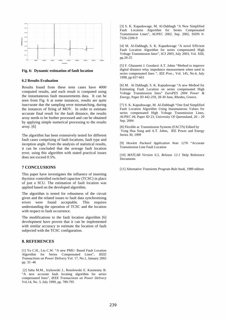
Fig. 6: Dynamic estimation of fault location 6.2 Results Evaluation
Results found from these tests cases have 4000 computed results, and each result is computed using the instantaneous fault measurements data. It can be seen from Fig. 6 at some instances, results are quite inaccurate due the sampling error mismatching, during the instances of firing of MOV. In order to estimate accurate final result for the fault distance, the results array needs to be further processed and can be obtained by applying simple numerical processing to the results array. [6] The algorithm has been extensively tested for different fault cases comprising of fault locations, fault type and inception angle. From the analysis of statistical results, it can be concluded that the average fault location error, using this algorithm with stated practical issues does not exceed 0.5%. 7 CONCLUSIONS This paper have investigates the influence of inserting thyristor controlled switched capacitor (TCSC) in place of just a SCU. The estimation of fault location was applied based on the developed algorithm.
The algorithm is tested for robustness of the circuit given and the related issues to fault data synchronising errors were found acceptable. This requires understanding the operation of TCSC and the location with respect to fault occurrence.
The modifications to the fault location algorithm [6] development have proven that it can be implemented with similar accuracy to estimate the location of fault subjected with the TCSC configuration.
8. REFERENCES [1] Yu C.H., Liu C.W. “A new PMU- Based Fault Location Algorithm for Series Compensated Lines”, IEEE Transactions on Power Delivery Vol. 17, No.1, January 2002 pp. 33 -46 [2] Saha M.M., Jzykowski J., Rosolowski E. Kasztenny B. “A new accurate fault locating algorithm for series compensated lines”, IEEE Transactions on Power Delivery Vol.14, No. 3, July 1999, pp. 789-795
[3] S. K. Kapuduwage, M. Al-Dabbagh “A New Simplified Fault Location Algorithm for Series Compensated Transmission Lines”, AUPEC 2002, Sep. 2002, ISDN 0-7326-2206-9 [4] M. Al-Dabbagh, S. K. Kapuduwage “A novel Efficient Fault Location Algorithm for series compensated High Voltage Transmission lines”, SCI 2003, July 2003, Vol. XIII, pp.20-25 [5] F. Ghassemi J. Goodarzi A.T. Johns “Method to improve digital distance relay impedance measurement when used in series compensated lines “, IEE Proc., Vol. 145, No.4, July 1998, pp 657-663 [6] M. Al Dabbagh, S. K. Kapuduwage “A new Method for Estimating Fault Location on series compensated High Voltage Transmission lines” EuroPES 2004 Power & Energy, Paper ID 442-259, 28-30 June, Rhodes, Greece. [7] S. K. Kapuduwage, M. Al-Dabbagh “One End Simplified Fault Location Algorithm Using Instantaneous Values for series compensated High Voltage Transmission Lines, AUPEC 04, Paper ID 23, University Of Queensland, 26 – 29 Sep. 2004
[8] Flexible ac Transmission Systems (FACTS) Edited by Yong Hua Song and A.T. Johns, IEE Power and Energy Series 30, 1999 [9] Hewlett Packard Application Note 1276 “Accurate Transmission Line Fault Location [10] MATLAB Version 6.5, Release 12-1 Help Reference Documents
[11] Alternative Transients Program Rule book, 1989 edition
239
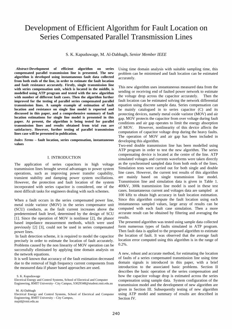
Development of Efficient Algorithm for Fault Location on Series Compensated Parallel Transmission Lines
S. K. Kapuduwage, M. Al-Dabbagh, Senior Member IEEE
Abstract-Development of efficient algorithm on series compensated parallel transmission line is presented. The new algorithm is developed using instantaneous fault data collected from both ends of the line, in order to estimate the fault location and fault resistance accurately. Firstly, single transmission line with series compensation unit, which is located in the middle, is modelled using ATP program and tested with the new algorithm with number of different fault cases. Then the algorithm further improved for the testing of parallel series compensated parallel transmission lines. A sample example of estimation of fault location and resistance on single line model is reported and discussed in this paper, and a comprehensive summary of fault location estimations for single line model is presented in this paper. At present, the algorithm is being tested for parallel transmission lines and results obtained from trial run are satisfactory. However, further testing of parallel transmission lines case will be presented in publication.
Index Terms – fault location, series compensation, instantaneous values
I. INTRODUCTION
The application of series capacitors in high voltage transmission lines brought several advantages to power system operations, such as improving power transfer capability, transient stability and damping power system oscillations. However, the protection and fault location of the system incorporated with series capacitor is considered, one of the most difficult tasks for engineers dealing with such schemes. When a fault occurs in the series compensated power line, metal oxide varistor (MOV) in the series compensator unit (SCU) conducts, as the fault current increases above the predetermined fault level, determined by the design of SCU [1]. Since the operation of MOV is nonlinear [2], the phasor based impedance measurement methods, which were used previously [2] [3], could not be used in series compensated power lines. In fault detection scheme, it is required to model the capacitor precisely in order to estimate the location of fault accurately. Problems caused by the non linearity of MOV operation can be successfully eliminated by applying time domain analysis on the network equations. It is well known that accuracy of the fault estimation decreased due to the removal of high frequency current components from the measured data if phaser based approaches are used. S. K. Kapuduwage Electrical Energy and Control Systems, School of Electrical and Computer Engineering, RMIT University– City Campus, [email protected] M. Al-Dabbagh Electrical Energy and Control Systems, School of Electrical and Computer Engineering, RMIT University – City Campus, [email protected]
Using time domain analysis with suitable sampling time, this problem can be minimised and fault location can be estimated accurately. This new algorithm uses instantaneous measured data from the sending or receiving end of faulted power network to estimate the voltage drop across the capacitor accurately. Then the fault location can be estimated solving the network differential equation using discrete sample data. Series compensation can be mainly catalogued in to series capacitor (C) and its protecting devices, namely metal oxide varistor (MOV) and air gap. MOV protects the capacitor from over voltage during fault conditions and air gap operates to limit the energy absorption of MOV. However, nonlinearity of this device affects the computation of capacitor voltage drop during the heavy faults. The operation of MOV and air gap has been included in developing this algorithm. Two-end double transmission line has been modelled using ATP program in order to test the new algorithm. The series compensating device is located at the centre of the line. ATP simulated voltages and currents waveforms were taken directly as the synchronised sampled data from both ends of the lines. Simulation tests were carried out for both single and double line cases. However, the current test results of this algorithm are mainly based on single transmission line model. Transmission line and simulation data is given in Table 1. 400kV, 300k transmission line model is used in these test cases. Instantaneous current and voltages data are sampled at 100 kHz to obtain high accuracy in fault location estimation. Since this algorithm compute the fault location using each instantaneous sampled values, large array of results can be computed with each fault case simulation. Then a more accurate result can be obtained by filtering and averaging the results. The presented algorithm was tested using sample data collected form numerous types of faults simulated in ATP program. Then fault data is applied to the proposed algorithm to estimate the location of fault. It was observed that the average fault location error computed using this algorithm is in the range of 0.2%. A new, robust and accurate method, for estimating the location of faults of a series compensated transmission line using time domain signals is introduced in this paper, with a brief introduction to the associated basic problems. Section II describes the basic operation of the series compensation and how the capacitor voltage drop is estimated across the series compensation using sample data. System configuration of the transmission model and the development of new algorithm are given in Section III. Subsequently testing of new algorithm using ATP model and summary of results are described in Section IV.
240
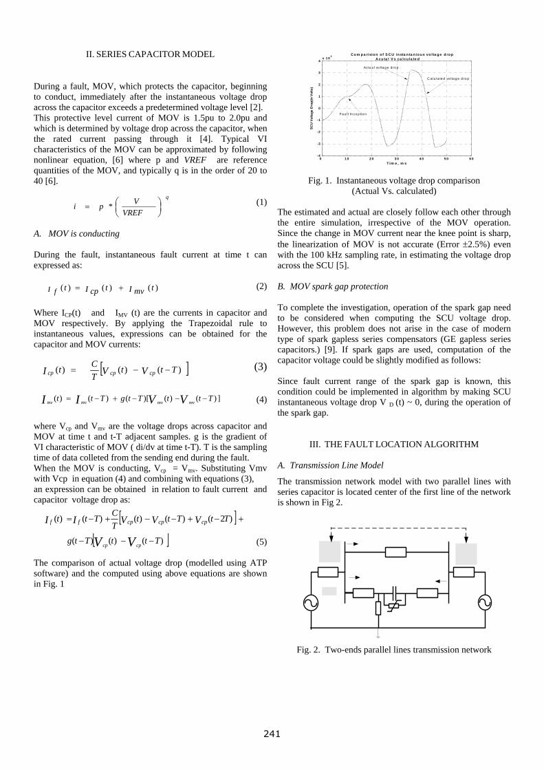
0 1 0 2 0 3 0
II. SERIES CAPACITOR MODEL
4 0 5 0 6 0-4
-3
-2
-1
0
1
2
3
4x 1 0 5
T im e , m s
SCU
Vol
tage
Dro
p(in
Vol
ts)
Co m p a risio n o f S C U in sta n ta n io u s vo lta g e d ro p A cu ta l V s ca lcu la te d
Fa u lt In ce p tio n
Actu a l vo lta g e d ro p
C a lu la te d vo lta g e d ro p
During a fault, MOV, which protects the capacitor, beginning to conduct, immediately after the instantaneous voltage drop across the capacitor exceeds a predetermined voltage level [2]. This protective level current of MOV is 1.5pu to 2.0pu and which is determined by voltage drop across the capacitor, when the rated current passing through it [4]. Typical VI characteristics of the MOV can be approximated by following nonlinear equation, [6] where p and VREF are reference quantities of the MOV, and typically q is in the order of 20 to 40 [6].
(1) A. MOV is conducting During the fault, instantaneous fault current at time t can expressed as:
(2)
Where ICP(t) and IMV (t) are the currents in capacitor and MOV respectively. By applying the Trapezoidal rule to instantaneous values, expressions can be obtained for the capacitor and MOV currents:
(3)
(4)
where Vcp and Vmv are the voltage drops across capacitor and MOV at time t and t-T adjacent samples. g is the gradient of VI characteristic of MOV ( di/dv at time t-T). T is the sampling time of data colleted from the sending end during the fault. When the MOV is conducting, Vcp = Vmv. Substituting Vmv with Vcp in equation (4) and combining with equations (3), an expression can be obtained in relation to fault current and capacitor voltage drop as:
(5) The comparison of actual voltage drop (modelled using ATP software) and the computed using above equations are shown in Fig. 1
Fig. 1. Instantaneous voltage drop comparison (Actual Vs. calculated)
⎟⎠⎞
⎜⎝⎛=
VREFVpi
q
* The estimated and actual are closely follow each other through the entire simulation, irrespective of the MOV operation. Since the change in MOV current near the knee point is sharp, the linearization of MOV is not accurate (Error ±2.5%) even with the 100 kHz sampling rate, in estimating the voltage drop across the SCU [5]. B. MOV spark gap protection ) To complete the investigation, operation of the spark gap need to be considered when computing the SCU voltage drop. However, this problem does not arise in the case of modern type of spark gapless series compensators (GE gapless series capacitors.) [9]. If spark gaps are used, computation of the capacitor voltage could be slightly modified as follows: [ ])()()( Ttt
TCt VVI cpcpcp −−=
Since fault current range of the spark gap is known, this condition could be implemented in algorithm by making SCU instantaneous voltage drop V D (t) ~ 0, during the operation of the spark gap.
])()()[()()( TttTtgTtt VVII mvmvmvmv −−−+−=
III. THE FAULT LOCATION ALGORITHM A. Transmission Line Model
The transmission network model with two parallel lines with series capacitor is located center of the first line of the network is shown in Fig 2.
[ ] +−+−−+−= )2()()()()( TtTttTCTtt VVVII cpcpcpff
[ ])()()( TttTtg VV cpcp−−−
Fig. 2. Two-ends parallel lines transmission network
(I mv)()( ttI cptI f +=
241
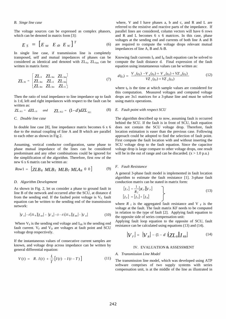
B. Singe line case The voltage sources can be expressed as complex phasors, which can be denoted in matrix form [3]:
(6) In single line case, if transmission line is completely transposed, self and mutual impedances of phases can be considered as identical and denoted with ZLA, ZLAm can be written in matrix form:
(7) Then the ratio of total impedance to line impedance up to fault is 1:d, left and right impedances with respect to the fault can be written as:
(8) C. Double line case In double line case [8], line impedance matrix becomes 6 x 6 due to the mutual coupling of line A and B which are parallel to each other as shown in Fig 2. Assuming, vertical conductor configuration, same phase to phase mutual impedance of the lines can be considered predominant and any other combinations could be ignored for the simplification of the algorithm. Therefore, first row of the new 6 x 6 matrix can be written as:
(9)
D. Algorithm Development
As shown in Fig. 2, let us consider a phase to ground fault in line B of the network and occurred after the SCU, at distance d from the sending end. If the faulted point voltage is VF, fault equation can be written to the sending end of the transmission network:
(10) Where VS is the sending end voltage and ISB is the sending end fault current. VF and VD are voltages at fault point and SCU voltage drop respectively. If the instantaneous values of consecutive current samples are known, and voltage drop across impedance can be written by general differential equation:
(11)
where, V and I have phases a, b and c, and R and L are referred to the resistive and reactive parts of the impedance. If parallel lines are considered, column vectors will have 6 rows and R and L becomes 6 x 6 matrices. In this case, phase voltages at the sending end and currents of both line A and B are required to compute the voltage drops relevant mutual impedances of line A, B and A-B.
[ ]EEEE scsbsaT
S =
Knowing fault currents IS and IR fault equation can be solved to compute the fault distance d. Final expression of the fault equation using instantaneous values can be written as:
)()()()()()()(
00
00000
tVZtVZtVZtVtVtV
tdRS
RDRS
+++−
= (12)
⎥⎥⎥
⎦
⎤
⎢⎢⎢
⎣
⎡
=
ZLZLZLZLZLZLZLZLZL
ZLAAmAm
AmAAm
AmAmA
A1 where t0 is the time at which sample values are considered for this computation. Measured voltages and computed voltage drops are 3x1 matrices for a 3-phase line and must be solved using matrix operations. E. Fault point with respect SCU dZLdZL AAand )1( 1112 −=dZLZL AA 111 = The algorithm described up to now, assuming fault is occurred behind the SCU. If the fault is in front of SCU, fault equation does not contain the SCU voltage drop. Therefore, fault location estimation is easer than the previous case. Following approach could be adopted to find the selection of fault point. First compute the fault location with and without inserting the SCU voltage drop to the fault equation. Since the capacitor voltage drop is large compare to other voltage drops, one result will be in the out of range and can be discarded. (x > 1.0 p.u.)
F. Fault Resistance [ ]001 MLAMLBMLBZLB RTSRRow =A general 3-phase fault model is implemented in fault location algorithm to estimate the fault resistance [1]. 3-phase fault conduction matrix can be stated in matrix form:
(13) where R f is the aggregated fault resistance and V F is the voltage at the fault. The fault matrix KF needs to be computed in relation to the type of fault [2]. Applying fault equation to the opposite side of series compensation unit:
[ ] [ ][ ]
[ ] [ ] [ ]III
VKR
I
RSF
FFf
F
+=
=1
[ ] [ ][ ] [ ] [ ][ ] [ ]VIVIV DRBBRSBBS ZLdZLd −−−=− )1(
Applying fault loop equation to the opposite of SCU, fault resistance can be calculated using equations (13) and (14).
[ ] [ ] [ ][ ]IZLVV RBBRF d )1( −−= (14)
IV. EVALUATION & ASSESSMENT
A. Transmission Line Model [ ])()()(.)( TtItI
TLtIRtV −−+= The transmission line model, which was developed using ATP
software comprises of two supply systems with series compensation unit, is at the middle of the line as illustrated in
242
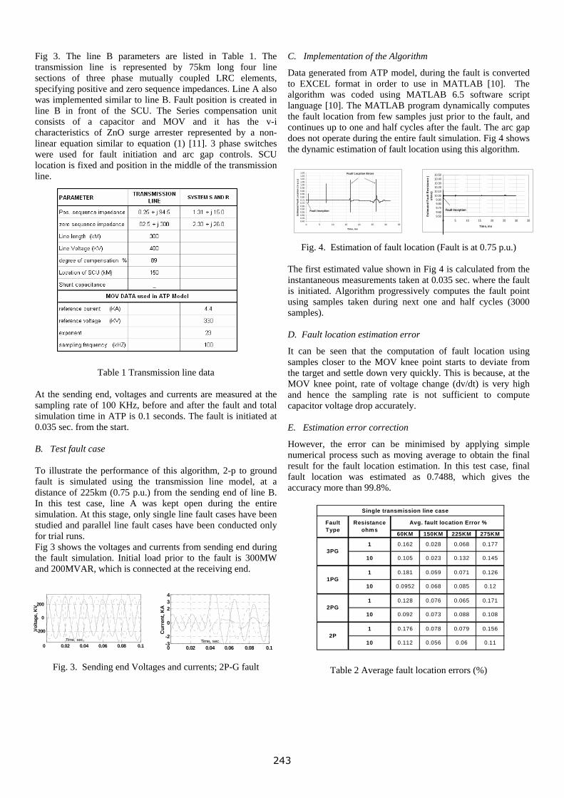
Fig 3. The line B parameters are listed in Table 1. The transmission line is represented by 75km long four line sections of three phase mutually coupled LRC elements, specifying positive and zero sequence impedances. Line A also was implemented similar to line B. Fault position is created in line B in front of the SCU. The Series compensation unit consists of a capacitor and MOV and it has the v-i characteristics of ZnO surge arrester represented by a non-linear equation similar to equation (1) [11]. 3 phase switches were used for fault initiation and arc gap controls. SCU location is fixed and position in the middle of the transmission line.
Table 1 Transmission line data At the sending end, voltages and currents are measured at the sampling rate of 100 KHz, before and after the fault and total simulation time in ATP is 0.1 seconds. The fault is initiated at 0.035 sec. from the start. B. Test fault case To illustrate the performance of this algorithm, 2-p to ground fault is simulated using the transmission line model, at a distance of 225km (0.75 p.u.) from the sending end of line B. In this test case, line A was kept open during the entire simulation. At this stage, only single line fault cases have been studied and parallel line fault cases have been conducted only for trial runs. Fig 3 shows the voltages and currents from sending end during the fault simulation. Initial load prior to the fault is 300MW and 200MVAR, which is connected at the receiving end.
Fig. 3. Sending end Voltages and currents; 2P-G fault
C. Implementation of the Algorithm
Data generated from ATP model, during the fault is converted to EXCEL format in order to use in MATLAB [10]. The algorithm was coded using MATLAB 6.5 software script language [10]. The MATLAB program dynamically computes the fault location from few samples just prior to the fault, and continues up to one and half cycles after the fault. The arc gap does not operate during the entire fault simulation. Fig 4 shows the dynamic estimation of fault location using this algorithm.
0.400.450.500.550.600.650.700.750.800.850.900.951.001.051.101.151.20
0 5 10 15 20 25 30 35
Time, ms
Estim
ated
Fau
lt Lo
catio
n ( i
n p.
u.)
Fault Inception
Fault Location Errors
9.509.609.709.809.90
10.0010.1010.2010.3010.4010.50
0 5 10 15 20 25 30 35
Time, ms
Estim
ated
Fau
lt R
esis
tanc
e (
ohm
s)
Fault Inception
Fig. 4. Estimation of fault location (Fault is at 0.75 p.u.)
The first estimated value shown in Fig 4 is calculated from the instantaneous measurements taken at 0.035 sec. where the fault is initiated. Algorithm progressively computes the fault point using samples taken during next one and half cycles (3000 samples). D. Fault location estimation error
It can be seen that the computation of fault location using samples closer to the MOV knee point starts to deviate from the target and settle down very quickly. This is because, at the MOV knee point, rate of voltage change (dv/dt) is very high and hence the sampling rate is not sufficient to compute capacitor voltage drop accurately. E. Estimation error correction
However, the error can be minimised by applying simple numerical process such as moving average to obtain the final result for the fault location estimation. In this test case, final fault location was estimated as 0.7488, which gives the accuracy more than 99.8%.
Single transmission line case
60KM 150KM 225KM 275KM
0.112
0.181
0.0952
0.128
0.092
0.145
0.068 0.177
0.176
0.085 0.12
0.071 0.126
0.056
0.068
0.06 0.11
0.079 0.156
0.088 0.108
0.065 0.171
0.059
0.076
0.073
0.0782P
1
10
Resistance ohms
1PG1
10
2PG1
10
Fault Type
Avg. fault location Error %
3PG1
10
0.162
0.105
0.028
0.023 0.132
0 0.02 0.04 0.06 0.08 0.1
-200
0
0 0.02 0.04 0.06 0.08 0.1-3-2
0
234
Cur
rent
, KA
Time, sec.
Table 2 Average fault location errors (%)
200
Volta
ge, K
V
Time, sec.
243
F. Algorithm assessment
In order to test the performance, over 50 wide verities of fault cases have been modelled in ATP, with single transmission line and average fault locations were computed using this algorithm and the results are summarised in Table 2.
Double transmission line case is being tested with the modified algorithm and results obtained from trial runs are showing encouraging results compares to single line case. Final results of these tests will be presented in publication.
Average fault location errors were computed by varying the fault inception angle 0, 45 and 90 degrees. According to the entries in the table, overall average fault location error is within 0.2%.
V. CONCLUSIONS
The algorithm presented in this paper provides a new accurate method for estimating fault location based on recording instruments assisted with GPS receivers providing accurate synchronised instantaneous fault from both ends of the series compensated transmission line. Since the fault location is repeatedly computed using the instantaneous measurements in this algorithm, accuracy of estimation is not affected by the fault resistance, time varying faults, type of SCU and source parameters. The emphasis in this paper has been on the proof of the efficiency of the developed algorithm for a mutually coupled R-L transmission line model. Future publications will take the effect of shunt capacitance into consideration.
VI. REFERENCES
[1] Yu C.H., Liu C.W. “A new PMU- Based Fault Location Algorithm for Series Compensated Lines”, IEEE Transactions on Power Delivery Vol. 17, No.1, January 2002 pp. 33 -46 [2] Saha M.M., Jzykowski J., Rosolowski E. Kasztenny B. “A new accurate fault locating algorithm for series compensated lines”, IEEE Transactions on Power Delivery Vol.14, No. 3, July 1999, pp. 789-795 [3] S. K. Kapuduwage, M. Al-Dabbagh “A New Simplified Fault Location Algorithm for Series Compensated Transmission Lines”, AUPEC 2002, Sep. 2002, ISDN 0-7326-2206-9 [4] M. Al-Dabbagh, S. K. Kapuduwage “A novel Efficient Fault Location Algorithm for series compensated High Voltage Transmission lines”, SCI 2003, July 2003, Vol. XIII, pp.20-25 [5] F. Ghassemi J. Goodarzi A.T. Johns “Method to improve digital distance relay impedance measurement when used in series compensated lines “, IEE Proc., Vol. 145, No.4, July 1998 [6] M. Al Dabbagh, S. K. Kapuduwage “A new Method foe Estimating Fault Location on series compensated High Voltage
Transmission lines” EuroPES 2004 Power & Energy, Paper ID 442-259, 28-30 June, Rhodes, Greece. [7] S. K. Kapuduwage, M. Al-Dabbagh “One End Simplified Fault Location Algorithm Using Instantaneous Values for series compensated High Voltage Transmission Lines, AUPEC 04, Paper ID 23, University Of Queensland, 26 – 29 Sep. 2004 [ 8] Jan Jzykowski, Eugenniusz Rosolowski, Murari Saha “Adaptive Digital Distance Algorithm for Parallel Transmission Lines”, Power Tech. Engineers Proceedings, 2003 IEEE, Bologra, Vol 2, 23-26 June 2003, PP 6 [9] Hewlett Packard Application Note 1276 “Accurate Transmission Line Fault Location [10] MATLAB Version 6.1, Release 12-1 Help Reference Documents [11] Alternative Transients Program Rule book, 1989 edition
244