* Corresponding author. Email: spg3@le.ac.uk

Fatigue tolerant design of rolling bearings

Simon P.A. Gill1* and Michael W.J. Lewis2

1Department of Engineering, University of Leicester,

University Road, Leicester, UK, LE1 7RH

2Formerly of the National Centre of Tribology, ESR Technology Ltd, Whittle House,

410 The Quadrant, Birchwood Park, Warrington WA3 6FW, UK.

Abstract

A quantitative method for assessing the influence of steel cleanliness on the fatigue life of rolling

bearing raceways is presented. The approach systematically accounts for the effect of the highly

variable stress state within raceways. Finite element analysis is used to determine the stress state in

the bearings. A fracture mechanics model for the safe stress amplitude as a function of inclusion size

is employed from Lewis and Tomkins, J Engng Tribology, 226(5) 389 (2012). The size and number of

large inclusions in a large volume of steel are estimated by the Generalised Pareto Distribution.

These three elements are combined to determine the failure probability of the raceway in an

example rolling bearing. A sensitivity analysis to the various microstructural input parameters is

conducted. It is found that the size distribution of the larger inclusions is the most important factor

in controlling the fatigue resistance of rolling bearings, and that residual stresses must be considered

to produce realistic predictions.

Keywords: fatigue; rolling bearings; statistics of extreme values; failure; steel cleanliness;

generalised Pareto distribution.

2

Nomenclature

𝑎 inclusion radius

𝑎0 & 𝑎1 minimum and maximum sizes of potentially damaging inclusions

𝑐 & 𝑑 major and minor semi-axes of the elliptical contact area

𝑐0 Lundberg-Palmgren index

𝑓(𝑎) volume fraction of raceway containing particles of size greater than 𝑎

𝑓𝐹 volume fraction of the raceway containing inclusions that will lead to fatigue failure

ℎ Lundberg-Palmgren depth-weighting index.

𝑙 raceway length

𝑛 Generalised Pareto Distribution exponent

𝑝𝑚𝑎𝑥 maximum contact pressure between the two contacting surfaces

𝑧 stress weighted average depth

𝑧0 depth of the maximum orthogonal shear stress

𝐴 cross-sectional area of the raceway

𝐴𝑐𝑜𝑛 total contact area

𝐶𝐸 a measure of the contacting bodies net compliance

𝐸1& 𝐸2 Young’s moduli of the ball and raceway

𝐻𝑉 Vickers hardness of the raceway

𝐾𝐷 a measure of the contacting bodies radii

𝐿10 basic rating life

𝑁𝑒 is the number of cycles survived raised to the power of the Weibull index

𝑁𝐹 average number of damaging inclusions in the raceway

𝑁𝑃 total number of potentially damaging inclusions in the raceway

𝑃 applied load

𝑃(𝑎) probability of an inclusion of size greater than 𝑎

𝑃𝐹 probability of a bearing failing due to damaging inclusions

𝑃𝑢 fatigue limit load

3

𝑅 maximum/minimum stress ratio

𝑅1& 𝑅1′ radii of the ball

𝑅2& 𝑅2′ radii of the raceway

𝑆𝑠 percentage of a population surviving

Δ𝑆 survivial probability of a volume Δ𝑉

𝑆𝑙𝑖𝑚𝑖𝑡 limit stress (in MPa)

𝑉0 total volume of the raceway

𝜆0 number of inclusions per unit volume in the material

𝜈1& 𝜈2 Poisson’s ratios of the ball and raceway

𝜙(𝑎) probability density of inclusions of size 𝑎

𝜎𝑒 von Mises effective stress

𝜎𝑟𝑒𝑠 residual stress in the surface of the raceway𝜏 shear stress amplitude exceeding the

fatigue limit

𝜏0 is the maximum orthogonal shear stress

𝜏𝑢 shear stress fatigue limit

4

1. Introduction

Lifing methods for rolling element fatigue were developed by Lundberg and Palmgren in the 1940s

and 50s by analysis of many hundreds of tests on small bearings at contact stresses well in excess of

2500MPa [1, 2]. Under these conditions, significant cyclic strain-induced metallurgical changes occur

[3]. These changes consist of the formation of white etching areas (WEAs) and dark etching areas

(DEAs) close to the running surface that are orientated at specific angles.

It was also found that significant compressive residual stresses are developed with protracted

running at these elevated stresses. However, it is difficult to state whether this would be beneficial

to life under stresses less than 2500MPa without proof from testing.

In view of the distribution in time to appearance of the first spall, Lundberg and Palmgren expressed

bearing fatigue in terms of L10 life, that is, the life that 90% of bearings would achieve under

nominally identical loading and lubrication regimes.

However, at more modest contact stresses that are typical of industrial bearings (1200 to 1800MPa),

no such metallurgical changes are seen, which leads to the question whether Lundberg and

Palmgren’s methodology would equally apply.

Sub-surface fatigue crack initiation predominantly takes place upon non-metallic inclusions that are

inevitably formed during the steel making process. Whilst modern bearing steels are significantly

cleaner than those tested by Lundberg and Palmgren, crack initiation can still take place on

inclusions, should they be located in the stressed contact zone.

It has been mainly assumed that the largest inclusion in a bearing raceway will be the one that is the

cause of sub-surface initiated fatigue failure. However, this does not take into account the

probability that this inclusion is in the most highly stressed area. It is possible that smaller but more

commonly found particles could be the source of fatigue initiation, as they will have a more

significant chance of being in the high stress region. Hence it is necessary to combine knowledge of

the stress state in the component with an understanding of the distribution of particle sizes within

the steel, the latter depending upon the steel cleanliness. This is particularly important in rolling

bearings, where only a small volume of the raceway experiences very high stresses, but a much

larger region experiences intermediate, but still potentially damaging, levels of stress.

The assessment of a bearing’s resistance to fatigue requires the input of three factors. Firstly, an

analysis of the stress state in the body is required. This is where the geometry and loading conditions

are incorporated into the model, as described in section 3. The other two factors describe the

material and its response to fluctuating loads. So secondly, a model for the fatigue properties of the

material, particularly the fatigue limit stress as a function of inclusion size, is required. This is

discussed in section 4. Thirdly, a statistical model for the distribution of inclusions throughout the

material as a function of their size must also be supplied.

This paper demonstrates this process for a rolling bearing of a given geometry. The output of this

process is the probability of eventual fatigue failure of the bearing raceway as a function of the

loading conditions. A sensitivity analysis is performed in section 6 to determine which of the

5

required input parameters is most important in determining the fatigue tolerance of the prescribed

design.

6

2. Current fatigue life methods

(a) Conventional approach

Rolling bearings are usually selected on the basis of a percentage of failures in an application within

a prescribed number of revolutions. Lundberg and Palmgren [1, 2] formulated a theory of fatigue

failure based upon Weibull probability [4] and thus proposed a method to calculate rolling bearing

life. Their life prediction model was based upon the equation

ln (1

𝑆𝑆) ≈ 𝑁𝑒 (

𝜏0𝑐0

𝑧0ℎ ) 𝑐𝑧0𝑙 (1)

where 𝑆𝑠 is the percentage of a population surviving, 𝑁𝑒is the number of cycles survived raised to

the power of the Weibull index, 𝜏0 is the maximum orthogonal shear stress, 𝑐0 is the Lundberg-

Palmgren index, 𝑧0 is the depth of the maximum orthogonal shear stress and ℎ is the Lundberg-

Palmgren depth-weighting index. The stressed volume 𝑉 is given by 𝑎𝑧0𝑙, where 𝑎 is the contact

major semi-axis and 𝑙 is the raceway length.

Substituting for the applied bearing loads, the following equation was obtained for the basic rating

life

𝐿10 = (𝐶

𝑃)

𝑝 (2)

where 𝑝 is an exponent (= 3 for ball bearings and 10/3 for roller bearings). It can be seen that eqn

(2) makes no provision for material structure or cleanliness, depending solely upon the basic

dynamic rating 𝐶 and the equivalent load 𝑃.

This equation was adopted by ANSI/AFBMA in 1978 and by ISO in 1990 [5]. Revisions to

ANSI/AFBMA Std-9 and Std-11 in 1990 [6, 7], as well as Ref 5, included factors 𝑎1, 𝑎2 and 𝑎3 to

account for different levels of reliability, material fatigue properties and lubrication quality. Factors

𝑎2 and 𝑎3 are usually combined to give a factor 𝑎23 that is a function of materials and lubrication

through the parameter𝜅 = 𝜈/𝜈1, the ratio of actual to required viscosity. It is limited to a maximum

value of 2.5.

Using the basic rating life methodology of Lundberg and Palmgren, the Society of Tribologists and

Lubrication Engineers (STLE) have adopted different independent factors, as summarised by Zaretsky

[8]. These factors cover bearing material, melting practice, metalworking, oil filtration level and

misalignment, amongst others.

(b) Fatigue limit approach

As a development of bearing life methodology, Ioannides and Harris [9] proposed a fatigue strength

approach, similar to that in structural fatigue. Thus a fatigue limit was introduced according to the

following equation by means of a shear stress fatigue limit 𝜏𝑢.

ln (1

𝛥𝑆) ≈

𝑁𝑒(𝜏−𝜏𝑢)𝑐

𝑧ℎ Δ𝑉 (3)

7

where Δ𝑆 is the survivial probability of a volume Δ𝑉, 𝜏 is the shear stress amplitude exceeding the

fatigue limit and 𝑧 is the stress weighted average depth. Whilst shear stress is used in eqn (3), an

alternative such as von Mises stress is equally applicable. This approach suggests that there is an

applied stress below which fatigue failure should not occur such that bearing life becomes infinite.

In support of the approach, Ioannides and Harris analysed results from rotating beam, torsional

beam and reversed bending beam tests with good agreement [9]. They also carried out a small

number of tests on 6309 deep groove ball bearings under two different steel qualities and

lubrication conditions (high and low , where 𝜆 is the ratio of oil film thickness to combined surface

finish of the surfaces).

They concluded that values of the shear stress fatigue limit 𝜏𝑢 = 300 and 350MPa applied to the bad

and good quality steels, whilst values of von Mises stress 𝜎𝑢𝑀= 519 and 606MPa were

correspondingly obtained. Applying a conversion factor of 0.55 for von Mises stress applicable to

roller bearings, this equates to maximum contact stresses of 950 and 1100MPa respectively.

The work of Ioannides and Harris was extended by Harris and Barnsby [10] in which a stress-life

factor 𝑎𝑆𝐿 was proposed to modify the basic rating life. This factor includes, but is not limited to,

fatigue endurance limit, sub- and surface-initiated failures, residual stress, hoop stress, oil film

thickness, lubricant contamination and surface tractions. The stress-life factor also includes failures

of rolling elements, ignored in the work of Lundberg and Palmgren.

Harris and Barnsby carried out a much more significant test programme reported in Ref [10] with a

variety of bearing types up to a pitch diameter of 388.5mm in materials including AISI 52100,

VIMVAR M50, case-hardening and induction hardening steels. Endurance testing showed a mean

von Mises fatigue limit stress of 684MPa for AISI 52100, stated to be a conservative value.

The approach adopted by Harris and Barnsby has been incorporated in the ASMELife software

program [11]. Within this software it is possible to select a value for the fatigue limit stress for

specific materials that reflects their metallurgy and cleanliness.

Recently, ISO 281 [12] has adopted a similar approach that considers the effects of lubricant

cleanliness and viscosity as well as the concept of an endurance limit. The latter is introduced as a

fatigue limit load 𝑃𝑢 (or 𝐶𝑢) so historically the concept of an endurance limit (or fatigue strength) has

been adopted for the lifing of rolling element, so the approach to be described below is a natural

development of this.

3. Stress analysis

(a) Finite Element model

The original application of fatigue tolerant analysis [13] utilised an analytical solution for the stress

field in the component (a plate with a hole). Here the analysis is conducted within the more flexible

framework of the finite element method. A rolling bearing is a good application to consider due to

the very wide variety of stress histories experienced by different elements of the raceway. The

geometry of a representative section of a large ball bearing is shown in Fig. 1a. Only a single ball

acting on a section of the outer raceway is considered as the contact stress field between the ball

8

and the raceway is very localised. The convex radius of the ball is 31.75 mm, the concave track radius

is 33.66mm, such that the osculation is 1.06 (or 53%), and the concave outer race radius is 910mm.

The exact cross-sectional dimensions of the raceway should not be important, as long as the contact

stress field is not significantly affected by the proximity of the external boundaries. The elastic

properties of the ball and the raceway are assumed to be the same, with a Young’s modulus of 210

GPa and a Poisson’s ratio of 0.3. Exploiting the symmetry of the problem, only a quarter of the

geometry needs to be modelled, as shown in Fig. 1b. A suitable range of uniformly distributed

displacements are applied normal to the flat, horizontal surface of the truncated ball to press the

ball into the raceway. The total load is subsequently calculated from the reaction force on this

surface, and is typically in the range of 10-80kN.

The finite element mesh is refined near the contact in an area defined by an ellipsoid. Due to the

curvature of the raceway, the contact zone is not axisymmetric, with the contact size across the

raceway being much larger than the contact size in the rolling direction. The variation in the von

Mises stress within the ball and the raceway is shown in Fig. 1b for a large applied load. The

maximum von Mises stress occurs a small distance below the centre of the contact.

(a) Fatigue tolerance method

The output required from this stress analysis for the evaluation of the fatigue tolerance of the

bearing outer raceway is determined as follows. As the ball moves around the raceway, any cross-

section of the raceway will experience the same fluctuating stress state as the ball passes over it.

The maximum stress amplitude of this fluctuation will occur when the centre of the ball is within the

cross-sectional plane, as shown in Fig. 1b. Firstly, we identify the cross-sectional area of the raceway

as the area 𝐴, as shown in Fig. 1a. The total volume of the raceway 𝑉0 can then be determined by

sweeping this area through 360o about the centre of the bearing such that

𝑉0 = 2𝜋 ∫ 𝑟𝑑𝐴𝐴

(4)

where 𝑟 is the distance from the centre of the bearing to a point within the outer raceway cross-

section. The objective of the stress analysis is to determine the fraction of this volume that has a von

Mises effective stress 𝜎𝑒 that is above a given stress 𝑆. The logical expression

𝜎𝑒 > 𝑆 = {1 𝑖𝑓 𝑡𝑟𝑢𝑒

0 𝑖𝑓 𝑓𝑎𝑙𝑠𝑒 (5)

is used to determine the swept volume in which the condition 𝜎𝑒 > 𝑆 is satisfied

𝑉(𝑆) = 2𝜋 ∫ (𝜎𝑒 > 𝑆)𝑟𝑑𝐴𝐴

. (6)

This is then normalised to define the volume fraction of the raceway in which 𝜎𝑒 > 𝑆

𝑓(𝑆) =𝑉(𝑆)

𝑉0. (7)

This function is plotted in Fig. 2a for the range of applied loads considered, from 1.6kN up to 80kN.

The curves become increasingly smooth as the load rises as the stress field extends over more finite

9

elements in the simulation and is more accurately represented by the discretised field. As one would

expect, the volume fraction above a certain stress level increases as the applied load is increased.

(b) Comparison with analytical solution

An analytical solution for the problem of two, doubly curved surfaces in contact is given in Roark’s

Formulas for Stress and Strain [14] and is widely used in the assessment of bearings. Therefore it is

of interest to see how this compares with the results of the finite element solution. For small

deformations, the analytical solution states that the shape of the elliptical contact area is given by

𝑐 = 𝛼(𝑃𝐾𝐷𝐶𝐸)1

3 𝑑 = 𝛽(𝑃𝐾𝐷𝐶𝐸)1

3 (8)

where 𝑐 and 𝑑 are the major and minor semi-axes of the elliptical contact area, such that the total

contact area is given by 𝐴𝑐𝑜𝑛 = 𝜋𝑐𝑑, and 𝑃 is the applied load, 𝐾𝐷 =1.5

1

𝑅1+

1

𝑅2+

1

𝑅1′ +

1

𝑅2′

is a measure of

the contacting bodies radii, and 𝐶𝐸 =1−𝜈1

2

𝐸1+

1−𝜈22

𝐸2 is a measure of their compliance. Here 𝐸1 = 𝐸2 =

210 𝐺𝑃𝑎 and 𝜈1 = 𝜈2 = 0.3. The two convex (positive) radii of the ball are 𝑅1 = 𝑅1′ = 31.75 𝑚𝑚

and the two concave (negative) radii of the raceway are 𝑅2 = −1.06𝑅1 and 𝑅2′ = −910 𝑚𝑚. The

two dimensionless constants can then be interpolated from a table of values defined by the value of

𝐾𝐷 such that 𝛼 = 3.00 and 𝛽=0.46 [14]. The maximum contact pressure between the two surfaces

is given by

𝑝𝑚𝑎𝑥 =1.5𝑃

𝐴𝑐𝑜𝑛= 𝜂𝑃

1

3 (9)

where 𝜂 is a geometrical constant defined by (8). The stresses in the raceway are expected to scale

with the contact pressure so that the von Mises effective stress 𝜎𝑒 is also proportional to 𝑃1

3. The

size of the stress contours in the cross-section (see Fig. 1b) will scale with the dimensions of the

contact radius. Thus the width and height of the stress field will scale as 𝑃1

3, and hence the area

contained by a particular stress contour will scale as 𝑃2

3.

To compare the simulation results with the above solution, Fig. 2a is re-plotted in Fig. 2b with the

axes renormalized such that, if the analytical solution is always valid, the curves should all collapse

onto the same master curve. The renormalizations are such that the measure of stress becomes 𝑆

𝑝max, and the measure of volume fraction becomes

𝑓(𝑆)

𝑃23

. The particular value of the volume fraction

is only relative, and depends on the size of the raceway cross-section adopted. Curves are only

plotted for four selected loads for clarity. The curves for intermediate loads lie proportionally

between those shown. It is clear from Fig. 2b that the curves do not exactly collapse on to a single

master curve, although the general scaling is roughly applicable. This is because the analytical

solution is only valid for small contacts. It is noted that for similar calculations by the authors of

contact between an identical ball and a flat surface under the same range of loads, the curves do

collapse much more precisely onto the same curve.

The relationship between the maximum contact pressure and the maximum von Mises stress is

given to be 𝑆max

𝑝𝑚𝑎𝑥= 0.557 for a cylinder contacting a flat substrate [15]. The constant of

10

proportionality is not easily defined for the general case of two doubly curved surfaces in contact,

but it is found that it is about 0.65 for a load of 32kN, and that it increases steadily with the applied

load, reaching a value of 0.68 at 80kN. This represents a significant difference of around 20% from

the cylinder case and hence shows that it is not a simple matter of employing a single master curve

for all contact problems. Values of about 0.63 are cited in the literature.

As one might expect, the stress field varies in shape as well as magnitude as the geometry changes.

The increase in the ratio of von Mises to contact stress with load is anticipated to be due to effects

of large deformations. With a small osculation, typical in bearing applications, the contact area

between the ball and the raceway expands quickly with the applied load. The contact pressure

between the two objects is normal to the surface. For small loads, this is almost entirely in the

(vertical) direction of the applied load, but as the contact area enlarges, the horizontal component

becomes more significant, as the ball starts to touch the side walls of the raceway.

(c) Effect of residual stress

The raceways of some rolling bearings are surface hardened, typically by induction hardening or

carburising. This is often used to gain high surface hardness whilst maintaining a tougher core. This

process induces a compressive residual stress in the near-surface of the component, which is

generally found to greatly improve its fatigue resistance. Therefore, it is necessary to consider the

contribution from residual stresses to see whether results are comparable to service experience.

Exact details about the residual stress field are unknown, but it is expected to be compressive,

reasonably uniform to a certain distance below the treated surface, and parallel to the plane of this

surface. Further away from the surface the residual stress must be tensile in order to ensure overall

force equilibrium. Fig. 3a shows the variation in the von Mises stress field in the cross-section

beneath the ball centre. Here it is assumed that a uniform compressive residual stress field exists to

a depth sufficient to cover the entirety of the high stress region, and that the orientation of the

surface above this region is sufficiently close to the horizontal (𝑥 − 𝑦 plane) that it can be assumed

to act entirely within this plane. Therefore, in the absence of specific detailed information, a simple

representation of the residual stress field is to replace the stress components in the horizontal plane

𝜎𝑥 and 𝜎𝑧 by (𝜎𝑥 − 𝜎𝑟𝑒𝑠) and (𝜎𝑧 − 𝜎𝑟𝑒𝑠), where 𝜎𝑟𝑒𝑠 = 400𝑀𝑃𝑎 is taken to be the magnitude of

the (compressive) near-surface residual stress field. The von Mises stress in the presence of the

residual stress is then defined as

𝜎𝑒𝑟𝑒𝑠 = √

1

2[(𝜎𝑥 − 𝜎𝑧)2 + (𝜎𝑥 − 𝜎𝑦 − 𝜎𝑟𝑒𝑠)

2+ (𝜎𝑧 − 𝜎𝑦 − 𝜎𝑟𝑒𝑠)

2+ 6(𝜏𝑥𝑦

2 + 𝜏𝑥𝑧2 + 𝜏𝑦𝑧

2 )] (10)

Fig. 3b shows the difference between the stress field in the presence of the residual stress,

calculated using (10), and the original stress field, shown in Fig. 3a. The residual stress is applied

everywhere, such that the unstressed (blue) regions in Fig.3a now have an increased stress level of

400MPa. This is unphysical but irrelevant, as the increase in the stress in these regions is still much

too small to initiate fatigue and hence they do not play any part in the overall calculation. The

relevant observation in Fig. 3b is that the area where the von Mises stress is reduced by the value of

the applied residual stress, 400MPa, completely covers the high stress area in Fig. 3a. This is where

fatigue will be initiated. Plotting the equivalent stress curves of Fig.2a show that the addition of the

residual stress field effectively just translates the high stress portion of the stress curve to the left,

11

such that a good approximation of the consequences of the residual stress field are obtained by

simply replacing 𝑆 by (𝑆 − 𝜎𝑟𝑒𝑠) on the horizontal axis. This is a simplified model, but introducing a

more sophisticated model will not have an observable qualitative effect on the final results.

4. Fatigue properties of the material

Having characterised the fluctuating stress state in the raceway, it is now necessary to relate the

state of stress in the volume to its propensity for initiating fatigue. It is assumed that fatigue initiates

at inclusions in the steel. Lewis and Tomkins [16] have proposed (based upon the work of Murakami

[17]) the following relationship between the size of an inclusion and the limit stress amplitude for

eventual fatigue failure

𝑆𝑙𝑖𝑚𝑖𝑡(𝑎) = 1.63(𝐻𝑉+120)(

1−𝑅

2)

𝛼

(0.49𝜋𝑎2)1

12

(11)

where the limit stress is given in MPa, 𝐻𝑉 = 750 is the Vickers hardness of the steel, 𝑅 = −1 is the

max/min stress ratio and 𝛼 = 0.226 + 𝐻𝑉x10−4. The inclusions are assumed to be ellipsoidal with

semi-axes 𝑎 and 𝑏 with 𝑏/𝑎=0.49 such that the cross-sectional area of the particles is 𝜋𝑎𝑏 or

0.49𝜋𝑎2. Equation (11) is plotted in Fig. 4. If the stress amplitude is below the line then no fatigue

will be initiated. If the stress amplitude is above the line, then fatigue failure will occur eventually.

It is now possible to re-map the horizontal stress axis in Fig. 2b using (11), 𝑆(𝑎), to calculate the

volume fraction above the limit stress, 𝑓(𝑎), as a function of the inclusion size. Fig. 5 shows the

volume fraction of the raceway that experiences stress amplitudes sufficiently large to initiate

fatigue in particles of size 𝑎 and above for different applied loads. Here the size of the ellipsoidal

particles is defined to be the largest radius which is roughly equivalent to the smallest diameter for

the assumed aspect ratio. As the load increases, larger proportions of the raceway volume

experience stresses which will activate a greater range of particles sizes.

5. Microstructural description

Figure 5 defines the fraction of the raceway in which an inclusion of a particular size has the

potential to act as a site for the initiation of fatigue failure. It is now necessary to combine this with a

description of the particle size distribution in the steel to determine the probability of finding an

inclusion of a potentially damaging size in a sufficiently stressed region of the raceway. It is not

possible to determine the probability of finding such large inclusions using a brute force approach,

as the large number of micrographics samples that would need to be examined to have confidence

that statistically significant numbers of such particles had been detected would be beyond practical

analysis. The size distribution is therefore usually interpreted from a smaller, more manageable,

number of micrographs using the statistics of extreme values [18-21]. There are a number of

different approaches to this problem [18]. In this paper we adopt the Generalised Pareto

Distribution (GPD) [13,18], where here it is expressed in the following form

𝑃(𝑎) = (𝑎1−𝑎

𝑎1−𝑎0)

𝑛 (12)

12

This form assumes that there is always a maximum size for any inclusions that can ever be found in a

sample, 𝑎1 . It also assumes that inclusions below a specific threshold size, 𝑎0, will never be

potentially damaging and do not need to be considered in the analysis. Therefore we are interested

in particles of size 𝑎0 ≤ 𝑎 ≤ 𝑎1. The exponent 𝑛 is the third fitting parameter for the distribution.

The probability 𝑃(𝑎) is therefore the cumulative probability of finding inclusions of a potentially

damaging size, 𝑎. Typical values for the threshold and maximum inclusion sizes are 𝑎0 = 5 microns

and 𝑎1 = 30 microns. The distribution function (12) is plotted in Fig. 6a for a range of exponent

values. The meaning of these distributions is often more easily interpreted from the probability

density function (PDF)

𝜙(𝑎) = −𝑑𝑃

𝑑𝑎=

𝑛

𝑎1−𝑎0(

𝑎1−𝑎

𝑎1−𝑎0)

𝑛−1 (13)

which defines the frequency of occurrence of inclusions of a particular size. The PDFs for the

distributions illustrated in Fig. 6a are shown in Fig. 6b. They demonstrate that a uniform distribution

of particles sizes is expected for 𝑛 = 1, i.e. there is equal chance of finding particles of any size in the

considered range, whilst for 𝑛 < 1 there is a greater chance of finding large particles than small

ones. This is not anticipated to be the case, and therefore one requirement on the exponent is that

𝑛 > 1. As the value of 𝑛 increases, the probability of large inclusions occurring becomes more and

more unlikely. The value of 𝑛 = 11 is typical of the values previously considered [13].

6. Probability of failure – a sensitivity analysis

The stress distribution in the raceway has been combined with the fatigue properties of the

material, and is summarised in Fig. 5. This is now amalgamated with the microstructural picture of

the inclusions in the material provided by Fig. 6b to determine the overall probability of failure of

these components. Firstly, it is necessary to define the number of potentially damaging inclusions,

with sizes 𝑎0 ≤ 𝑎 ≤ 𝑎1, that are estimated to occur in the body of the raceway. Hence we let λ0 be

the number density of these inclusions in the steel under consideration. Given that we have

determined the total volume of the raceway, V0, in (4), the total number of potentially damaging

inclusions in the raceway is NP = λ0V0. However, these inclusions can only actually lead to the

initiation of fatigue damage if they are in a region of the raceway that experiences a sufficiently high

enough stress to activate it. Combining Fig. 5 and Fig. 6b, the volume fraction of the raceway

containing actually damaging inclusions that will lead to fatigue failure is

𝑓𝐹 = ∫ 𝑓(𝑎)𝜙(𝑎)𝑑𝑎𝑎1

𝑎0. (14)

This is the sum over the product of the volume fraction of the raceway, 𝑓(𝑎), containing particles

which experience stress amplitudes above the stress limit (11), and the probability that inclusions of

this critical size exist, 𝜙(𝑎). The average number of actually damaging inclusions that might be

expected to be found in the raceway is therefore 𝑁𝐹 = 𝑁𝑃𝑓𝐹. The chances of finding a particular

number of damaging inclusions in a body obeys the Poisson distribution, which gives the probability

of failure for an event that occurs on average with a frequency 𝑁𝐹 such that

𝑃𝐹 = 1 − exp (−𝑁𝐹) (15)

13

The predictive capacity of this expression is now investigated. The first factor to be considered is the

effect of a residual stress. This is then followed by a study of the sensitivity of this rolling bearing to

the four microstructural parameters: 𝑎0, 𝑎1, 𝑛 and 𝜆0. In all studies, the volume of the raceway is

𝑉0 = 0.00454 𝑚3. Apart from the final study, we assume that 𝜆0 = 1 inclusion per mm3 such that the

total number of potentially damaging inclusions is 𝑁𝑃=4,540,000. For the geometry considered, in

(9) 𝜂 = 5.95 𝑥 107 𝑁2

3/𝑚2 , such that the maximum contact pressures are 1.28, 1.61 and 1.85 GPa

at applied loads of 10, 20 and 30 kN respectively.

(a) Residual stress, 𝜎𝑟𝑒𝑠

Fig. 7 shows the failure probability (15) as a function of the load applied to the ball for the case

where a compressive 400MPa residual stress is superimposed on the raceway stress state, and the

case where no residual stress is considered. It is clear that including the residual stress is very

important, and that it has a huge effect on the typical fatigue failure load of the bearing. Fig.7

indicates that one bearing in a thousand will fail by fatigue if the applied load is 12kN without a

residual stress. The allowable applied load for this failure rate is increased to 31kN if the 400MPa

residual stress is included. This is a reasonable value for the failure load of bearings of this type, and

therefore the effects of the residual stress are included in all the subsequent analyses.

(b) The exponent 𝑛

Three different values for the exponent 𝑛 are chosen and the results are plotted in Fig. 8. The

smaller the exponent, the greater the frequency of large inclusions in the size distribution. The

failure probability shows that for the lowest value, 𝑛 = 2, a raceway is predicted to suffer from

fatigue failure as soon as the applied load reaches the critical value at which only the largest

inclusions will cause eventual failure. This is because the probability of finding such inclusions is

reasonably large. This probability decreases significantly as 𝑛 is increased. An increase to 𝑛 = 5 only

makes a noticeable difference in the onset of fatigue failure occurring if a failure probability for the

bearing of one in ten or above is allowable. The largest value considered, 𝑛 = 11, is used in [18] and

demonstrates that the fatigue life of the component can be significantly increased for a given

applied load if the number of large inclusions can be made sufficiently infrequent. Even though large

inclusions still occur, it is then unlikely that they will be found in the small highly stressed region of

the raceway. For 𝑛 = 11 the probability of finding an inclusion of size greater than 21 microns is one

in a hundred thousand. Hence 𝑛 = 11 is considered to represent an extremely clean steel.

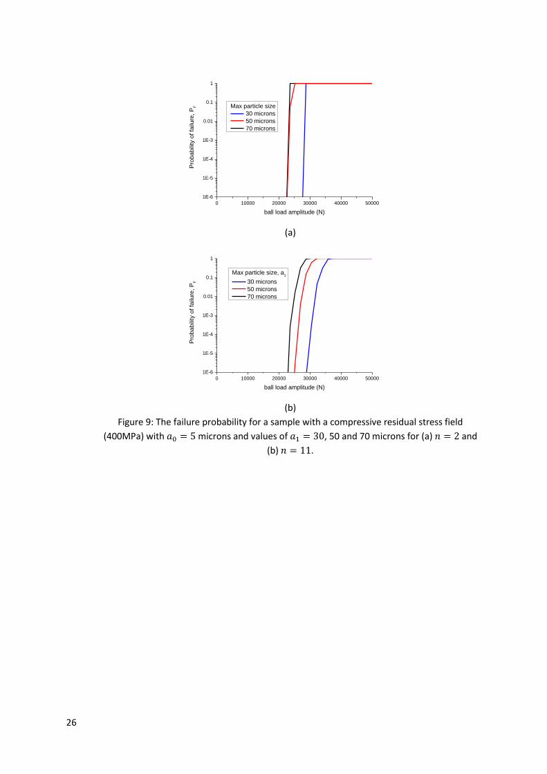
(c) Maximum inclusion size, 𝑎1

Three maximum particle sizes are considered: 𝑎1=30, 50 and 70 microns. The effect of varying the

maximum inclusion size is shown for two cases in Figs. 9a and 9b in which 𝑛 = 2 and 𝑛 = 11. As

expected, both figures demonstrate that the failure probability increases as the maximum inclusion

size in the steel is increased. As in Fig. 8, the case of 𝑛 = 2 in Fig. 9a illustrates a sharp transition

from no chance of failure to 100% chance of eventual failure once the applied load reaches the limit

at which the highest stress is large enough to activate the largest inclusions in the body. The

similarity between 𝑎1=50 microns and 𝑎1=70 microns shows that the stress limit (11) is not sensitive

to very large inclusion sizes. Fig. 9b is likely to be more representative of the inclusion distribution in

an actual clean steel. It shows a clearer differentiation between the three cases, as the chances of

finding the larger inclusions in the highly stressed region becomes less likely. As in Fig.7, for 𝑎1=30

14

microns one in a thousand raceways are predicted to suffer fatigue failure for an applied load of

31kN. As the maximum inclusion size increases to 50 and 70 microns, this applied load decreases to

26kN and 24kN respectively. This is a significant difference in load bearing capacity, with a variation

of about 25% between the two extreme cases.

(d) Number of inclusions, 𝑁𝑃

The number of potentially damaging inclusions in the raceway, 𝑁𝑃 = 𝜆0𝑉0, can be varied by either

changing the density of inclusions within the steel, 𝜆0, or the size of the raceway, 𝑉0. Fig. 10 shows

the effect of reducing the number of potentially damaging inclusions in the steel by a factor of 10

and 100. Assuming the dimensions of the raceway cannot be changed, this would be achieved in

investing in a significantly cleaner, and more expensive, steel. It is clear that for a low acceptable

failure probability of 10−3 the bearing is fairly insensitive to changes in this parameter, with an order

of magnitude change in the number of inclusions only increasing the allowable applied load for the

bearing by 1kN. For a higher acceptable failure probability of 0.1 a larger increase of 2.5kN is

possible. Hence it would certainly appear, for this very large rolling bearing, that the benefits of

decreasing the number of inclusions in the steel are relatively small compared to the additional

effort and expense involved. In addition, it is also useful to note that it is probably not normally

necessary to expend extensive micrographic effort in determining the parameter 𝜆0 to a high degree

of accuracy.

7. Conclusions

The fatigue tolerance assessment process of Yates et al [13] has been applied to the practical case of

fatigue in the raceway of rolling bearings. The technique has been extended to the case of more

general geometries and loading conditions through application of the finite element method. The

case study of a particular rolling bearing is illustrated in some detail. It is found that finite element

analysis is required for accurate simulation of doubly curved surfaces which undergo large

deformations.

The final output of the model is the probability of eventual fatigue failure of the raceway as a

function of the applied ball load. This depends on the material models for the dependence of the

fatigue limit on inclusion size and the distribution of inclusion sizes within the steel. With a residual

stress of 400MPa the threshold for rolling bearing fatigue failure at a probability of 0.001 are shown

to be in a range of applied loads from 24-32kN depending on inclusion sizes and numbers. This

corresponds to a range of contact pressures from 1.7 to 1.9 GPa. The sensitivity of the failure

probability is investigated with respect to the input parameters. It is found that incorporation of a

residual stress field is extremely important in the analysis of bearing raceways, with a compressive

400MPa residual stress increasing the one in a thousand failure load from 12kN to 31kN. It is

acknowledged that the residual stress model is very simplistic, and that further work should be done

to represent this in a more realistic manner.

However, the general conclusions are not expected to change, unless the high stress region moves

below the near-surface residual stress zone. As expected, decreasing the frequency of very large

inclusions is beneficial to the life of the component. This is particularly true for bearing raceways,

15

where only a small volume of the body experiences the highest stresses, so the inclusions found in

this region have a lower chance of being large enough to initiate eventual fatigue failure. The total

number of inclusions is shown to be less important, as long as the chances of encountering large

inclusions is sufficiently rare. However, the primary output of this work is a quantification of the

effects of rare, large inclusions, including exactly what rare and large mean in this context.

References

1. Lundberg G and Palmgren A. Dynamic capacity of rolling bearings. Acta Polytechnica, Mechanical Engineering Series. Royal Swedish Academy of Engineering Sciences, Vol 1, No 3, pp 7, 1947.

2. Lundberg G and Palmgren A. Dynamic capacity of roller bearings. Acta Polytechnica, Mechanical Engineering Series. Royal Swedish Academy of Engineering Sciences, Vol 2, No 4, pp 96, 1952.

3. Zwirlein O and Schlicht H. Rolling contact fatigue mechanisms - accelerated testing vs field performance. Rolling Contact Fatigue Testing of Bearing Steels. ASTM STP 771 pp 358-379. 1982.

4. Weibull W. A statistical representation of fatigue failures in solids. Acta Polytechnica, Mechanical Engineering Series. Royal Swedish Academy of Engineering Sciences, Vol 5, No 9, pp 49, 1949.

5. ISO 281-1. Rolling bearings - dynamic load ratings and rating life. International Standards Organisation. 1990.

6. ANSI/AFBMA Std 9-1990. Load ratings and fatigue life for ball bearings. ANSI/AFBMA.

7. ANSI/AFBMA Std 11-1990. Load ratings and fatigue life for roller bearings. ANSI/AFBMA.

8. Zaretsky E. STLE life factors for rolling bearings. STLE. 1992.

9. Ioannides E and Harris T A. A new fatigue life model for rolling bearings. ASME Jour of Tribology, Vol 107, pp 367. July 1985

10. Harris T A and Barnsby R M. Life ratings for ball and roller bearings. I Mech E Jour of Eng Tribology. Proc I Mech Eng, Vol 215, Part J, pp 577. 2001.

11. Barnsby R et al. Life ratings for modern rolling bearings - a design guide for the application of International Standard ISO 281/2. Trib Vol 14. 2003.

12. ISO 281. Rolling bearings - dynamic load ratings and rating life. International Standards Organisation. 2007.

13. Yates J R, Shi G, Atkinson H V, Sellars C M and Anderson C W. Fatigue tolerant design of steel

components based on the size of large inclusions. Fatigue Fract Engng Mat Struct Vol 25, pp

667, 2002.

14. Young W C, Budynas R G and Sadegh A M. Roark's Formulas for Stress and Strain. McGraw-

Hill Inc, Eighth Edition, 2012.

15. Harris T A and Kotzalas M N. Essential Concepts of Bearing Technology. CRC Press, Fifth

Edition, 2006.

16. Lewis M W J and Tomkins B. A fracture mechanics interpretation of rolling bearing fatigue.

Proc IMechE Part J: J Engineering Tribology, Vol 226, pp 389, 2012.

16

17. Murakami Y. Metal fatigue: effects of small defects and non-metallic inclusions. Elsevier 2002.

18. Shi G, Atkinson H V, Sellars C M and Anderson C W. Application of the generalized Pareto

distribution to the estimation of the size of the maximum inclusion in clean steels. Acta

Mater. Vol 47, pp 1455, 1999.

19. Shi G, Atkinson H V, Sellars C M and Anderson C W. Comparison of extreme values statistical

methods for predicting maximum inclusion size in clean steels. Ironmaking Steelmaking, Vol

26, pp 23, 1999.

20. Atkinson H V, Shi G, Sellars C M and Anderson C W. Statistical prediction of inclusion sizes in

clean steels. Mat. Sci. Tech., Vol 16, pp 1175, 2000.

21. Anderson C W, Shi G, Atkinson H V and Sellars C M. The precision of methods using the

statistics of extremes for the estimation of the maximum size of inclusions in clean steels.

Acta Mater., Vol 48, pp 4235, 2000.

17

Figure captions

Figure 1 : (a) Geometry of the roller bearing, considering a single ball on the outer raceway, and (b)

stress analysis of the ball in contact with the raceway. A quarter of the problem can be analysed due

to symmetry. The load is applied downwards in the y-direction on the upper flat surface. The

stresses shown are von Mises stresses. The ellipsoidal region around the contact area demarcates an

area of mesh refinement.

Figure 2 : Distribution of peak stress within the raceway volume. (a) The volume fraction above a

given stress 𝑆, 𝑓(𝑆), as a function of the stress 𝑆. As the applied load 𝑃 increases, the volume

fraction above a given stress increases. (b) Some of the profiles from (a) renormalized using

analytical contact theory. The profiles do not collapse onto precisely the same master curve,

indicating that the stress state under the indenter does not exactly scale with the load according to

Hertzian contact theory.

Figure 3: (a) Von Mises stress profile in the raceway cross-section, 𝜎𝑒. (b) The change in the von

Mises stress, 𝜎𝑒𝑟𝑒𝑠 − 𝜎𝑒, when a horizontal 400MPa compressive stress is incorporated into the von

Mises stress calculation. This shows that the (red) region where the highest stresses act in (a) is

completely covered by the (blue) region in (b) where the residual stress reduces the von Mises stress

by approximately 400MPa.

Figure 4: The fatigue limit stress (11) as a function of inclusion size.

Figure 5: Combining Fig. 2b and Fig. 4 gives the volume fraction of the raceway, 𝑓(𝑎), where the

stress is large enough to initiate fatigue from inclusions of size 𝑎.

Figure 6: The (a) cumulative probability GPD function (12), and (b) its probability density function

(13), for a threshold size of 𝑎0 = 5 microns, maximum size 𝑎1 = 30 microns, and various values of

the exponent 𝑛.

Figure 7: The failure probability for a sample with 𝑎0 = 5 microns, 𝑎1 = 30 microns, 𝑛 = 11, with a

compressive residual stress field (400MPa) and without (0 MPa).

Figure 8: The failure probability for a sample with 𝑎0 = 5 microns, 𝑎1 = 30 microns, a compressive

residual stress field (400MPa) for various values of 𝑛.

Figure 9: The failure probability for a sample with a compressive residual stress field (400MPa) with

𝑎0 = 5 microns and values of 𝑎1 = 30, 50 and 70 microns for (a) 𝑛 = 2 and (b) 𝑛 = 11.

Figure 10: The failure probability for a sample with a compressive residual stress field (400MPa) with

𝑎0 = 5 microns, 𝑎1 = 30 microns, 𝑛 = 11 for different values for the number of inclusions in the

raceway 𝑁𝑃.

18

(a) (b)

Figure 1 : (a) Geometry of the roller bearing, considering a single ball on the outer raceway, and (b)

stress analysis of the ball in contact with the raceway. A quarter of the problem can be analysed due

to symmetry. The load is applied downwards in the y-direction on the upper flat surface. The

stresses shown are von Mises stresses. The ellipsoidal region around the contact area demarcates an

area of mesh refinement.

Cross-sectional

area A

19

(a)

(b)

Figure 2 : Distribution of peak stress within the raceway volume. (a) The volume fraction above a

given stress 𝑆, 𝑓(𝑆), as a function of the stress 𝑆. As the applied load 𝑃 increases, the volume

fraction above a given stress increases. (b) Some of the profiles from (a) renormalized using

analytical contact theory. The profiles do not collapse onto precisely the same master curve,

indicating that the stress state under the indenter does not exactly scale with the load according to

Hertzian contact theory.

0 200 400 600 800 1000 1200 1400 1600 1800 2000

1E-4

1E-3

0.01

0.1

1

P=80kN

volu

me fra

ction w

ith

e>

S, f(

S)

stress, S (MPa)

P=1.6kN

0.0 0.1 0.2 0.3 0.4 0.5 0.6 0.7

-7

-6

-5

-4

-3

norm

alis

ed v

olu

me fra

ction, lo

g10(f

(S)/

P2

/3)

normalised stress, S/pmax

32kN

48kN

64kN

80kN

20

(a) (b)

Figure 3: (a) Von Mises stress profile in the raceway cross-section, 𝜎𝑒. (b) The change in the von

Mises stress, 𝜎𝑒𝑟𝑒𝑠 − 𝜎𝑒, when a horizontal 400MPa compressive stress is incorporated into the

von Mises stress calculation. This shows that the (red) region where the highest stresses act in

(a) is completely covered by the (blue) region in (b) where the residual stress reduces the von

Mises stress by approximately 400MPa.

21

Figure 4: The fatigue limit stress (11) as a function of inclusion size.

0 10 20 30 40 50

0

200

400

600

800

1000

1200

1400

eventual fatigue failure

limit s

tress a

mplit

ude, S

limit (

MP

a)

particle size, a (microns)

no fatigue failure

22

Figure 5: Combining Fig. 2b and Fig. 4 gives the volume fraction of the raceway, 𝑓(𝑎), where the

stress is large enough to initiate fatigue from inclusions of size 𝑎.

0 10 20 30 40 50

0.00

0.01

0.02

0.03

0.04

0.05

volu

me fra

ction w

ith

e>

Slim

it, f(

a)

particle size, a (microns)

32kN

48kN

64kN

80kN

23

(a)

(b)

Figure 6: The (a) cumulative probability GPD function (12), and (b) its probability density function

(13), for a threshold size of 𝑎0 = 5 microns, maximum size 𝑎1 = 30 microns, and various values of

the exponent 𝑛.

0 5 10 15 20 25 30

0.0

0.2

0.4

0.6

0.8

1.0

a1

P(a

>a

0)

particle size, a (microns)

n=11

n=2

n=1

n=0.5

a0

0 5 10 15 20 25 30

0.00

0.02

0.04

0.06

0.08

0.10

a1

pro

babili

ty d

ensity function, (a

i)

particle size, ai (microns)

n=11

n=2

n=1

n=0.5

a0

24

Figure 7: The failure probability for a sample with 𝑎0 = 5 microns, 𝑎1 = 30 microns, 𝑛 = 11,

with a compressive residual stress field (400MPa) and without (0 MPa).

0 10000 20000 30000 40000 50000

1E-6

1E-5

1E-4

1E-3

0.01

0.1

1

Pro

babili

ty o

f fa

ilure

, P

F

ball load amplitude (N)

Residual stress

0 MPa

400 MPa

25

Figure 8: The failure probability for a sample with 𝑎0 = 5 microns, 𝑎1 = 30 microns, a

compressive residual stress field (400MPa) for various values of 𝑛.

0 10000 20000 30000 40000 50000

1E-6

1E-5

1E-4

1E-3

0.01

0.1

1

Pro

babili

ty o

f fa

ilure

, P

F

ball load amplitude (N)

Size distribution

n<=2

n=5

n=11

26

(a)

(b)

Figure 9: The failure probability for a sample with a compressive residual stress field

(400MPa) with 𝑎0 = 5 microns and values of 𝑎1 = 30, 50 and 70 microns for (a) 𝑛 = 2 and

(b) 𝑛 = 11.

0 10000 20000 30000 40000 50000

1E-6

1E-5

1E-4

1E-3

0.01

0.1

1

Pro

babili

ty o

f fa

ilure

, P

F

ball load amplitude (N)

Max particle size

30 microns

50 microns

70 microns

0 10000 20000 30000 40000 50000

1E-6

1E-5

1E-4

1E-3

0.01

0.1

1

Pro

babili

ty o

f fa

ilure

, P

F

ball load amplitude (N)

Max particle size, a1

30 microns

50 microns

70 microns

27

Figure 10: The failure probability for a sample with a compressive residual stress field

(400MPa) with 𝑎0 = 5 microns, 𝑎1 = 30 microns, 𝑛 = 11 for different values for the

number of inclusions in the raceway 𝑁𝑃.

0 10000 20000 30000 40000 50000

1E-6

1E-5

1E-4

1E-3

0.01

0.1

1

Pro

babili

ty o

f fa

ilure

, P

F

ball load amplitude (N)

Particle number, NP

4,540,000

454,000

45,400