fast and robust algorithm to compute exact polytope parameter bounds

Mathematics and Computers in Simulation 32 (1990) 481-493 North-Holland

481

FAST AND ROBUST ALGORITHM TO COMPUTE EXACT POLYTOPE PARAMETER BOUNDS

S.H. MO

Jaguar Cars Ltd., Abbey Road, Whitley, Coventry CV.3 4LF, UK

J.P. NORTON

School of Electronic and Electrical Engineering, University of Birmingham, P.O. Box 363, Birmingham B15 2TT, UK

When bounds on the parameters of a linear-in-the-parameters model are computed, the exact feasible parameter set defined by the bounds (a polytope) is usually approximated by a simpler shape such as an ellipsoid. However, such simpler bounds may be much looser than the exact bounds. A new algorithm for updating the exact bounds is presented and compared with other recently published methods. Computational results illustrate exact polytope-bound updating by this algorithm from records of realistic length.

1. Introduction

The parameter-bounding approach to identifying models of dynamical systems [l-3] computes bounds on the model parameters from bounds on the error between model output and observed output. For example, if at sampling instant t we specify bounds

emin < e, < emax

on the error between observed output yI and the output ~$8 of the model

y, = fge + e I, t= 1, 2, 3, (2)

then we can infer bounds

c,: & c$e < c,+ on the p-vector 8 of parameters, where

(3)

c+ =y, - emin, c,: = y, - emax. (4)

For model (2), the bounds on 8 are parallel hyperplanes, normal to the known explanatory-variable vector c/J~. A sequence of observations yt to yN yields N pairs of such bounds. The active bounds define a polytope as the feasible parameter set $SN, so long as p or more are linearly independent. Any parameter values in 9,,, are consistent with all N observations and with the assumed model structure and the error bounds. For more general models, the parameter bounds will not be linear and 9 will not be a polytope. From here on, we consider only the linear case.

0378-4754/90/$03.50 0 1990 - Elsevier Science Publishers B.V. (North-Holland)

482 S. H. MO, J. P. Norton / Exact polytope parameter bow&

In some cases, 9 may be very complicated. Most previous work approximated 9 by a number of simpler shapes, symmetrical (ellipsoid [4], orthotope (box) [5]) or asymmetrical (simplex, pol t y ope with fixed number of faces [6]). To see why approximation might be necessary, consider the maximum number n of vertices of the p-dimensional ( p + q)-faced polytope

It can be shown that [7]

n ~ (;+lp/2lj + (;+[P/wj, (6) where [ ] and [ 1 are the round-down and round-up functions. According to (6), n might be large even for modest p and q. For example, n < 352 for p = 6 and q = 10, and n G 12397 for p = 8 and q = 20. It has also been conjectured [8] that the maximum number m of ( p - l)-faces of an n-vertex polytope in p dimensions is

i

Y2) “-P for p even,

n-(P+lw m = 2(,-p ) for p odd.

(7)

This is verified easily for p = 1, 2, 3 and n = p + 1; proofs for n = p + 2 and p + 3 are available [8]. If the conjecture is true, m = 680 for p = 6 and n = 20, for instance. These figures make the motive for simplifying 9 clear, but simpler bounds may well be much looser, so it is worth asking if, in practice, the exact bounds can be computed.

To update the exact polytope, 9, the active observation-induced parameter bounds must be identified at each stage. Using batch algorithms, the number of active bounds, and hence the number of vertices of 9, has been found usually to rise quite slowly with the number of observations [9,10]. The number depends, of course, on the distributions of C$ and e, but the rapidly decelerating rises found in Section 14 (for uniformly distributed 9 and e) are typical. Thus recursive algorithms to update the slowly lengthening list of active bounds are worth investigating. A new recursive active-bound-updating algorithm is described below, and compared with differently arranged but fundamentally similar algorithms already published [6,11-131.

2. Definition and properties of polytope

Definition 1. A polyhedral set 2% R’ p is the intersection of a finite family of closed half spaces of lRp [14].

Definition 2. A polytope 9 is the convex hull of its vertex set:

9= conv(~), whereV={u,,q ,..., u,} withuiERP,i=1,2 ,..., x.

Definition 2 will be relevant when we discuss the updating algorithm, but we should also see how the bounds (3) give a polytope. Let + be

3cq= {e]c,+ >,@>c,T}, 8, $BiiRP.

S. H. MO, J. P. Norton / Exact polytope parameter bounds 483

By Definition 1, 9 = f-l;“,,& is a polyhedral set. Every bounded polyhedral set is a polytope [14], so L% is a polytope (possibly the empty set) iff N >, p and p of the { t$, } are linearly independent. 9 is also convex, as the intersection of a finite family of convex sets is convex [14] and each q is convex since from (9)

(l-h)e,+he,E% VO<A<l vej, 8,E&. (IO)

If 2 is a supporting hyperplane of (i.e. bounds and has a point in) a closed convex set 9, F is called a face of Y [7]. We shall call a face of dimension k a k-face. A polytope has a finite number of faces, each a convex polytope [7]. If .F is a face of polytope B and 9 a face of 9, 3 is a face of 9 [14].

3. Representation of parameter-bounding polytope

Throughout the following sections, we consider the generic case, i.e. the bounding algorithm does not cater explicitly for degenerate or exceptional cases. The logic of the algorithm is such that treating non-generic cases as generic cases does not cause large errors.

The parameter-bounding polytope

where

can be represented by its O-faces (vertices) or ( p - l)-faces (bounding hyperplanes). To update the set V of vertices when a new observation is made, the vertices excluded by any new active bound must be identified, and new vertices formed where the new bound cuts existing bounds. Hence the vertices adjacent to (sharing a l-face with) each vertex u must be listed, and so must the ( p - l)-faces intersecting at u. Two approaches are possible. The adjacencies may be established anew at each step by calculation, as in [ll]. Alternatively, permanent lists may be kept of the adjacent vertices and intersecting faces for each vertex, updated as necessary [13]. This redundant description of the polytope takes more storage, but requires only logical operations to handle adjacencies. As a result (as discussed in Section 10) round-off errors do not lead to serious topological errors, whereas recalculation of adjacencies at each update is prone to round-off error [ll], discussed further in Sections 11 and 12.

The new exact polytope-updating algorithm described below keeps vertex-vertex (v-v) adjacency lists and vertex-face (v-f) lists. Figure I shows the lists for a single vertex, and Fig. 2 the complete polytope.

- vertqx label

coordinate v-v adjacency I

v-f adJ acency element 1 vertex label 1 face label 1

polytope vertexJ

I element 2 vertex label 2 face label 2

active-bound labels I_

label 1 laAe1 k I I

face label p . label 1 . . label x

element p vertex label p I , I co v-v v-if I co v&J v-f

Fig. 1. Description of a vertex by the exact polytope updating algorithm.

Fig. 2. Description of a polytope by the exact polytope updating algorithm.

484

4. Introduction of new

Let 3’ and .X-

S. H. MO, J. P. Norton / Exact polytope parameter bounds

bounds

be the half spaces induced by the latest observation yI:

.q+ = {e~~~e,(y,-e,,=c~), &-= B(#B>y,-em,,= 1 ct- > 03) and denote their boundaries by

h: = { 9 1 #e = c: } ) h, = {fl~c@=c;}. WI

The positions of all the vertices in V with respect to h: are indicated by a+, where

T a+= [c-q, a; )..., CXX’] ) a,? = c,+ - f#$;, i=l, 2 ,..., x. 05)

If a+ is non-negative, q is in g’; if negative, outside %+; if zero, in h:. When Z3-i is updated to gt, 9!_ 1 is not modified by $’ if a+ is entirely non-negative, ZBf is empty if a+ is all negative, and 3’ intersects and modifies gZ_ 1 if some but not all elements of a+ are negative. Similarly for q- with appropriate changes of signs; from here on, for brevity we shall discuss only &’ and omit the sign superscript.

The polytope is updated as follows. Hyperplane h, cuts .9-i, forming a new (p - 1)-face h: of 9,. Face h: can be regarded as the convex hull of its vertex set V * , in which each vertex is a vertex of 9t but not of gt_ i. Each l-face (edge) a( j, k) of 9(_ 1 is a convex combination of two adjacent vertices 4 and q:

Cqj, k)= {eIe=(l-h)o,+Xv,,O~X~l; 9, QkE_i} (16)

and may be found from the v-v lists. If an edge is cut by h,, the intersection is a vertex in V*. We may see whether c?( j, k) cuts h, by examining the positions of vertices q and u, with respect to h,. As in Fig. 3, &(j, k) cuts h, iff q. ET and v, G??*, i.e. iff a; > 0 and ak -C 0.

The new vertex UT satisfies

q&J: = c, ; q?=(l-h)u,+Xvj, O<A<l; (Yj>O, a,<0

so

The set ?lr* of new vertices is found by applying (18) to all pairs of adjacent vertices which pass the test in (17). The negative elements of a show which vertices from K_i deleted.

(17)

from <_, are to be

Fig. 3. Interpolation of a new vertex.


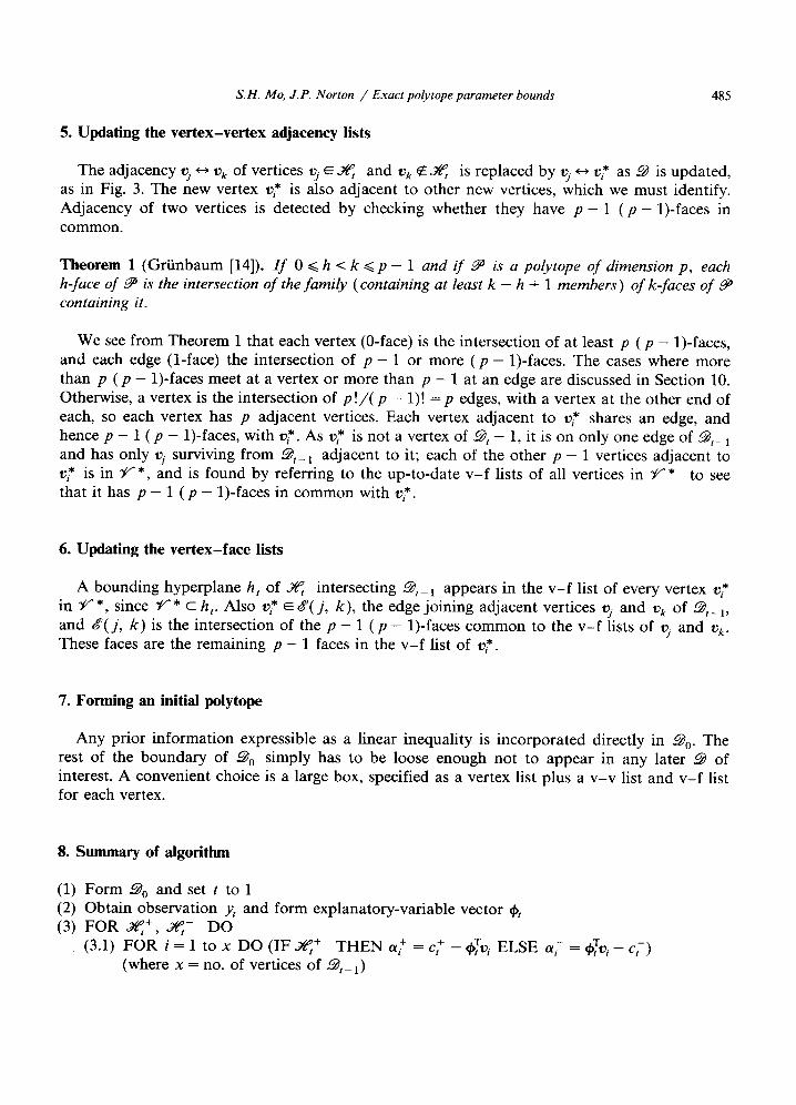
5. Updating the vertex-vertex adjacency lists

The adjacency U, f, u, of vertices 01 E q and v, CZ 3cq is replaced by 271~ u? as 9 is updated, as in Fig. 3. The new vertex uj* is also adjacent to other new vertices, which we must identify. Adjacency of two vertices is detected by checking whether they have p - 1 ( p - 1)-faces in common.

Theorem 1 (Griinbaum [14]). If 0 < h < k <p - 1 and if 9’ is a polytope of dimension p, each h-face of 9 is the intersection of the family (containing at least k - h + 1 members) of k-faces of B containing it.

We see from Theorem 1 that each vertex (O-face) is the intersection of at least p ( p - l)-faces, and each edge (l-face) the intersection of p - 1 or more ( p - l)-faces. The cases where more than p ( p - l)-faces meet at a vertex or more than p - 1 at an edge are discussed in Section 10. Otherwise, a vertex is the intersection of p!/( p - l)! = p edges, with a vertex at the other end of each, so each vertex has p adjacent vertices. Each vertex adjacent to 0;” shares an edge, and hence p - 1 ( p - I)-faces, with VT. As u: is not a vertex of 9* - 1, it is on only one edge of 9,-r and has only Us surviving from _9*_, adjacent to it; each of the other p - 1 vertices adjacent to u: is in V*, and is found by referring to the up-to-date v-f lists of all vertices in V* to see that it has p - 1 ( p - l)-faces in common with VT.

6. Updating the vertex-face lists

A bounding hyperplane h, of x intersecting ZB_ t appears in the v-f list of every vertex UT in V*, since V* c h,. Also uz* E &‘( j, k), the edge joining adjacent vertices 9 and u, of 9,-r, and &‘( j, k) is the intersection of the p - 1 (p - l)-faces common to the v-f lists of 9 and v,. These faces are the remaining p - 1 faces in the v-f list of UT.

7. Forming an initial polytope

Any prior information expressible as a linear inequality is incorporated directly in go. The rest of the boundary of go simply has to be loose enough not to appear in any later 9 of interest. A convenient choice is a large box, specified as a vertex list plus a v-v list and v-f list for each vertex.

8. Summary of algorithm

(1) Form 5B0 and set t to 1 (2) Obtain observation yt and form explanatory-variable vector & (3) FOR &+, q- DO

(3.1) FOR i = 1 to x DO (IF q’ THEN I_Y+ = c; - c#+; ELSE cui = $$u; - c;) (where x = no. of vertices of 9t _ 1)

486 S. H. MO, J. P. Norton / Exact polytope parameter bounds

(3.2) (3.3)

Form a = (IF 8’ THEN a+ ELSE a-) IF all elements of a are non-negative THEN

leave gt_ 1 unchanged; GOT0 (3.4) ELSE IF all elements of a are negative THEN

9, = 0; GOT0 (5) ELSE

(3.4)

(3.3.1) Find V* as in Section 4 (3.3.2) Form v-f lists for V* as in Section 6 (3.3.3) Form v-v lists for V* as in Section 5 (3.3.4) Update gt_l: adjoin Y* to V and delete vertices not in K CONTINUE

(4)

(5)

IF there are more observations THEN increment t; GOT0 (2)

ELSE STOP STOP

9. Example

Figure 4 shows an update of gt- 1 composed of half spaces

xi: o,>,o; x2: 0,a.o; 3q: e+o; x4: e1<3; &: &<2; %: 062

with p = 3. The new observation imposes

8: 38, + 2e, + e, G 5.

(b)

Fig. 4. Updating of exact polytope of parameter bounds.

Tab

le

I

Dol

vtoD

e is

.-

1

vert

ex1

vert

ex2

vert

ex3

vert

ex4

vert

ex5

vert

ex6

vert

ex7

vert

ex8

VI

w

vf

y w

vf

0,

w

vf

0,

w

vf

0,

w

vf

q

w

vf

0,

w

vf

u,

vv

vf

0 2

2 2

12

2 2

4 0

13

0 11

2 2

12

3 10

4

1 0

4 3

0 3

4 2

4 5

2 3

4 0

8 2

0 5

2 2

6 5

2 5

3 3

5 4

3 6

6 3

7 6

3 8

5 0

6 3

0 7

6 0

8 6

0 7

5

Tab

le

2

vert

ex1

vert

ex2

vert

ex3

vert

ex4

vert

ex5

u:

W

vf

s*

w

vf

6 w

vf

04

” w

vf

O

S*

w

vf

0 5

t 2

6 t

2 6

t 1

8 t

0 8

t

0 4*

2

0 l$

2

$ V

‘i+

1

2 6

1 2

v:

3

f cg

3

1 0:

6

0 $

6 0

0:

5 4

0:

5

Tab

le

3

poly

tope

SS

l

vert

ex1

vert

ex2

vert

ex3

vert

ex4

vert

ex5

vert

ex6

vert

ex7

vert

ex8

01

w

vf

4 w

vf

4

w

vf

0,

w

vf

u5

w

vf

qj

w

vf

u,

w

vf

u,

w

vf

0 7

t 2

8 t

2 8

t16

t 0

6 t

0 4

10

112

2 1

0220

32~4

1231

2132

5306

2032

s 5

311

6 0

2 6

0 5

5 f

4 5

0 7

5 0

8 3

0 7

6


The vertices, v-v and v-f lists are, as in Fig. 4(a), shown in Table 1. The set of edges, each sharingp-1=22-faces,isE={&i, &2, &3,...,&‘1;2}={1 t,2,2t,3,3t,4,4t,I,4t,6,6tt 7, 7 t, 8, 8 ++ 5, 1 ++ 5, 2 * 6, 3 * 7, 4 e S}. The algorithm now proceeds as follows:

Steps (3.1) (3.2). For 3, (Y is found using (15): a = [a1 a2 . * * asIT = [ -4 -6 - 10 -8 5 3 -1 llT so vertices 5, 6 and 8 are in & and will survive as vertices of gf. The discarded-vertex set is { ol, u,, v,, v,, v7 } . Checking through the edges and vertex pairs of Bt_ 1, we find that edges &h, &T, g9, &10 and Q,, intersect h,. Using (17) and (18), Y* can now be found (Fig. 4(b)):

Step (3.3.1).

Y-* = {r$(I, 5), q(2, 6), 173*(6, 7), $(7, 81, $+?4, 8>>

= {[o 0 $1) [2 0 11) [2: 01, [I 2 01, [o 2 :I}.

Steps (3.3.2) (3.3.3). The v-f list for each new vertex is formed next, then the v-v lists can be formed (see Table 2).

Step (3.3.4). 9l_1 is finally updated to 9l by collecting together the non-redundant vertices of 9 r_, and Y *. Vertices VT, UT and VT of .9_, become v_T, t.$ and 02 of 9(. The updated polytope (Fig. 4(c)) is shown in Table 3.

10. Round-off error and degenerate vertices

Two stages of the algorithm involve arithmetic; the calculation of a in Step 3.2 and the calculation of the new vertices in Step 3.3.1. The effects of round-off error are as follows. When $+ is being processed, rounding up of an element of a causes more of gl_ 1 to be included in the feasible region. If h, happens to be very close to a vertex of ~9_~, this can result in marginally redundant vertices being included in the updated active vertex set c;, with the result shown in Eg. 5. The algorithm will not detect such an occurrence, as it only updates the vertices and adjacency information, but will suffer no untoward consequences; the outcome of adjacency tests will not be misleading.

In Step 3.3.1, if h in (18) is rounded up, new vertices will be closer to the surviving vertex than they should be, and the updated polytope smaller. If A is rounded down, the polytope is larger than it should be. However, these errors do not affect the logic of the adjacency tests, except insofar as they make them apply to a slightly different polytope. Detection of adjacencies does not rely on precise new calculations at each updating stage.

When an element of a is rounded down, a smaller updated polytope results. Again such errors are insignificant and do not lead to large errors in the operation of the algorithm. However, repeated exclusion of feasible vertices and inclusion of infeasible vertices may cause noticeable cumulative error in 9 if 9 is ill conditioned (i.e. relatively thin in some direction).

When a, is calculated as zero for some vi, either (i) no other vertex is excluded by h,, u, is included in gt,, 99-I r‘l& = 91_1 and no updating action occurs; the worst that round-off can do is to prevent a minor clipping of L9_ 1, or (ii) at least one other vertex is excluded,

S. H, MO, J. P. Norton / Exact polytope parameter bounds 489

$S_i n% c g[,-i and the new polytope has U, as a vertex, but more edges and ( p - l)-faces meet at U, after the update than before, as illustrated by Fig. 6. The algorithm copes automati- cally with this eventuality. For each edge of 52-i containing vi and cut by h,, a new vertex u,* equal to U, is generated by (17) and (lg), and the adjacencies are found as usual. This process produces a number of coincident new vertices, each with the normal number of neighbours. That is, a new vertex at the intersection of p + q edges is represented by q + 1 new vertices, each the intersection of p edges. Figure 6 shows the situation for two coincident vertices. As the updating mechanism is insensitive to distance between vertices, the coincidence of vertices causes no difficulty. The only drawback is extra storage due to the redundancy. In practice the probability of coincident vertices is small enough for this problem to be negligible.

11. Exact bound updating using polyhedral cone

The recursive exact-polytope algorithm of Piet-Lahanier and Walter [ll-131 transforms 9 to a polyhedral cone V. This exact cone algorithm (e.c.a.) and the exact polytope algorithm (e.p.a.) described above were developed independently but have much in common. The e.c.a. writes the parameter bounds as homogeneous inequalities in ( p + l)-vectors

8’= [er ylTE lRp+’ (19)

with y positive (taken as 1 below). Half spaces 3cq+ and 3cq- are expressed as half spaces through the origin:

3+= (8’

where

I$,+‘Te’<o}, 2q = {e’~c#l-‘Te’~o},

- c, ‘I’> $q = [ -cg c;]‘. the feasible parameter set is the polyhedral cone

I t \

At sample instant t,

due to rwnd-off error

Fig. 5. Effects of round-off errors.


disiance= o -a

(a) (b) (cl

Fig. 6. Occurrence of a degenerate vertex.

The algorithm updates a matrix W whose columns are the edges of %‘, i.e. the vertices of 9. A new bound @i:‘@’ G 0 excludes edge i of %‘,_ 1 if element i of

(Y’ = yr,+;

is positive. If +i corresponds to active bound q in %ZZ_ 1 and m, is defined as

(23)

m4= lYr,$i,, (24)

then WZ,+, is zero if bounding hyperplane hi contains edge j of ‘ik; _ i. Edges k and 1 are adjacent iff they are both contained by at least p - 1 shared bounds and no other edge sharing those bounds intervenes. In its original form the adjacency test was not robust to round-off errors [11,12]. The present version uses a Boolean matrix to record the relationship between edges and supporting hyperplanes. Element (i, j) of this matrix is 0 if hyperplane j supports edge i of the cone and 1 otherwise. The adjacency and redundancy tests are thus logical operations and updating of the Boolean matrix does not require arithmetical operations [13]. The only arithmetical value affecting updating is then that of (Y’. The effect of rounding a small element of (Y’ to zero is similar to that described in Section 10 for the e.p.a.

The e.c.a. is rather more general than the e.p.a., which assumes each vertex to be the intersection of exactly p (p - l)-faces (and thus to have exactly p adjacent vertices), with the consequences described in Section 10. The e.c.a. makes no such assumption. The e.c.a. also allows the parameters to be unbounded in some directions; the updating mechanism of the e.p.a. does not cover that possibility. Finally, the e.c.a. is more elegant and may be implemented by a much more concise program.

12. Complete polytope updating

A third polytope-bounding algorithm is that of Broman and Shensa [6]. It updates the entire structure of the polytope, including faces of all dimensions below p. This complete polytope


algorithm (c.p.a.) is computationally expensive, so its authors suggest restricting the number of active bounds, obtaining an outer-bounding approximation 3 to 9. (The algorithm was originally intended for an application where p is small enough for computational expense not to be a critical factor.) On the other hand, the nature of the c.p.a. allows it to be coded very concisely.

The update starts by putting a box about 6, then cuts it successively with whichever remaining bound of the active bounds of a and the new one cuts most deeply, i.e. maximizes the perpendicular distance from any excluded vertex to the bound. The cutting is performed until the number of faces of & reaches the specified limit. For each cut, first the new O-faces are found from the new bound and knowledge of the sub-faces of the old l-faces, then the new l-faces, 2-faces,. . . , ( p - l)-faces are built up. In general, the k-faces are constructed by discarding the (k - l)-faces made redundant by the new bound and adding the new (k - l)-faces.

The method used to calculate the locations of new vertices is just as in the e.p.a. However, the determination of which faces can be discarded as redundant is quite different. The e.p.a. uses the adjacency information directly to identify redundant ( p - I)-faces, whereas the c.p.a. operates recursively in dimension, finding whether a (k - l)-face is redundant by checking if all that face’s (k - 2)-faces are redundant, for k = 2, 3,. . . , p.

13. Other possibilities

Many other methods could form the basis for polytope bounding. Redundant-constraint detection algorithms [C-17] can identify the active observation-induced bounds constituting the (p - l)-faces of the polytope. An algorithm for enumeration of all vertices of the polytope [l&223 can then be applied.

14. Numerical example

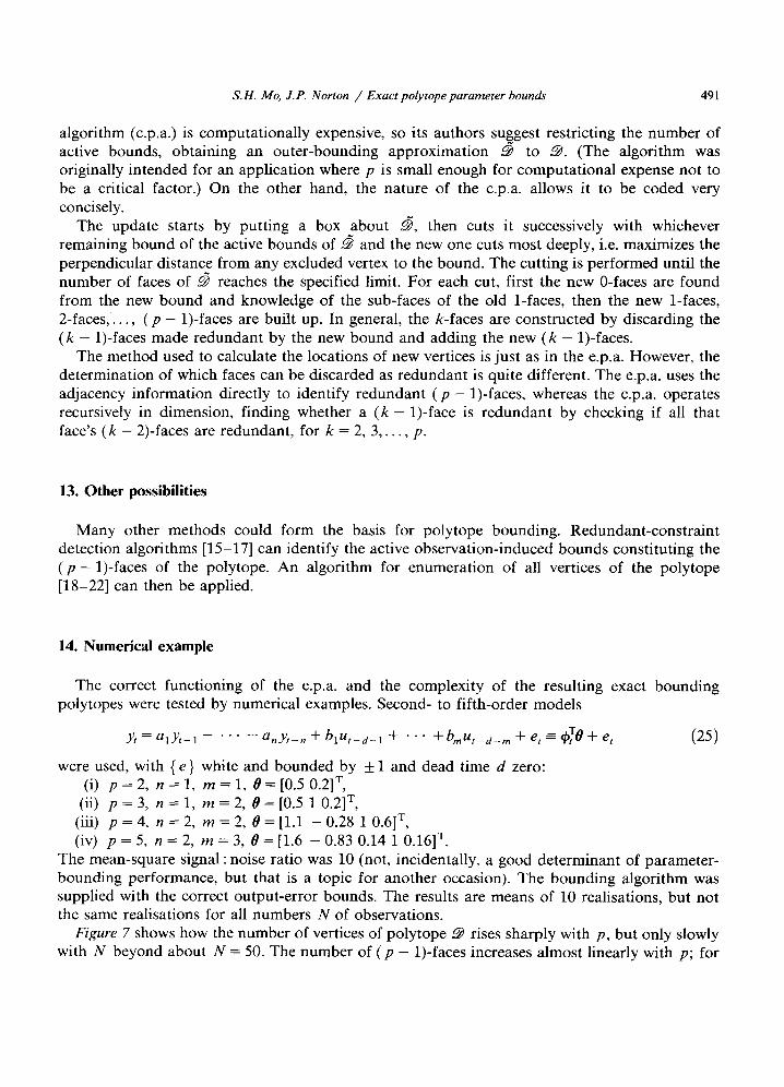
The correct functioning of the e.p.a. and the complexity of the resulting exact bounding polytopes were tested by numerical examples. Second- to fifth-order models

y, = a,~,_, - . + * - a,,~[-~ + b,u,_,_, + * . . + b,,,ut_d_m + e, = ($6 + e,

were used, with { e} white and bounded by + 1 and dead time d zero: (i) p = 2, n = 1, m = 1, B = [OS 0.21T,

(ii) p = 3, n = 1, m = 2, e = [OS 1 0.21T,

(25)

(iii) p = 4, n = 2, m = 2, B = [l.l - 0.28 1 0.61T, (iv) p = 5, n = 2, m = 3, 8 = Il.6 - 0.83 0.14 1 0.161T.

The mean-square signal : noise ratio was 10 (not, incidentally, a good determinant of parameter- bounding performance, but that is a topic for another occasion). The bounding algorithm was supplied with the correct output-error bounds. The results are means of 10 realisations, but not the same realisations for all numbers N of observations.

Figure 7 shows how the number of vertices of polytope 9 rises sharply with p, but only slowly with N beyond about N = 50. The number of ( p - l)-faces increases almost linearly with p; for


X10’

16 /O------

14 / ---0

12

10

p-0

8 i 0’ i

0 P=5 --- q p=4 -.-.-.-

x p=3 _-_-_----.

+ p=2

0 1 2 3 4 5 6 7 8 9 10 x 10’ No of observations N

x IO’ Well conditioned, 10M.C. runs, snr=lO, varying model order

a 24 I I 1 u22 - %I? 0’

/o------~~

I 20- ,o- -0”

- 0 p=5 ,18_ ---

hl6- o/ -0’ .--a----.-.__._,

- .-. ,o p=4 -.-.-.- k 14-

/o/

,,O--.-tl-. - x p=3

Lz :’ -/,~‘x___,_--x----x-

--------- ___x------_--_--______~:

O% ,/ : 8

-+ p=2

$J $$+-+-+~+-f--------

t 1 I 1 I 1 I I I

0 12 3 4 5 6 7 8 9 10 x10’ No. of observations N

Well conditioned, 10 M.C. runs, snr = 10, varying model order

Fig. 7. Complexity of exact bounding polytopes for various record lengths and model orders.

given p it rises very slowly beyond N = 50 or so, and may even decrease. These results, typical of our experience, indicate that the parameter-bounding polytope is often much less complicated than one might expect.

15. Conclusion

The three bound-updating algorithms provide different compromises between simplicity in theory and programming, economy in c.p.u. time and storage, and sensitivity to rounding error. Although the exact parameter-bounding polytope is very complicated in the worst case, it is often manageable in realistic examples. All the algorithms are recursive and potentially usable on line.

References

[l] E. Walter and H. Piet-Lahanier, Estimation of parameter bounds from bounded-error data: a survey, Math. Comput. Simulation 32 (5&6) (1990) 449-468 (this issue).

[2] J.P. Norton, Identification and application of bounded-parameter models, Automatica 23 (1987) 497-507. [3] J.P. Norton, An Zntroduction to Identification (Academic Press, New York, 1986).


[4] E. Fogel and Y.F. Huang, On the value of information in system identification-bounded noise case, Automatica

18 (1982) 229-238. [5] M. Milanese and G. Belforte, Estimation theory and uncertainty intervals evaluation in presence of unknown-

but-bounded errors, linear families of models and estimators, IEEE Trans. Automat. Control AC-27 (1982) 408-414.

[6] V. Broman and M.J. Shensa, A compact algorithm for the intersection and approximation of N-dimensional polytopes, Math. Comput. Simulation 32 (5&6) (1990) 469-480 (this issue).

[7] P. McMullen and G.C. Shephard, Convex Polytopes and the Upper Bound Conjecture (Cambridge University Press, London, 1971).

[8] D. Gale, On the number of faces of a convex polytope, Canad. J. Math. 16 (1964) 12-17. [9] S.H. MO and J.P. Norton, Parameter-bounding identification algorithms for bounded-noise records, Proc. ZEE-D

135 (1987) 127-132.

[lo] S.H. MO, Computation of bounded-parameter models of dynamical systems from bounded-noise records, Ph.D. thesis, School of Electronic & Electrical Eng., Univ. of Birmingham, 1989.

[ll] H. Piet-Lahanier, Estimation de parametres pour des modeles a erreur bornke, These de Doctorat en Sciences, Universite de Paris-Sud-Orsay, 1987.

[12] E. Walter and H. Piet-Lahanier, Exact and recursive description of the feasible parameter set for bounded error models, in: Proc. 26th IEEE Conference on Decision and Control, Los Angeles (1987) 1921-1922.

[13] H. Piet-Lahanier and E. Walter, Exact recursive characterization of feasible parameter sets in the linear case, Math. Comput. Simulation 32 (5&6) (1990) 495-504 (this issue).

[14] B. Grtinbaum, Conuex Polytopes (John Wiley and Sons, London, 1967). [15] T.H. Mattheiss, An algorithm for determining irrelevant constraints and all vertices in system of linear

inequalities, Oper. Res. 21 (1973) 247-260. [16] J. Telgen, Redundancy and Linear Programs, Mathematical Centre Tracts 137 (Mathematisch Centrum Amster-

dam, Amsterdam, 1981). [17] J. Telgen, Identifying redundant constraints and implicit equalities in system of linear constraints, Management

Sci. 29 (1983) 1209-1222. [18] M.L. Balinski, An algorithm for finding all vertices of convex polyhedral sets, J. SIAM 9 (1961) 72-89. [19] B.V. Hohenbalken, Finding faces of polytopes by simplicial decomposition part I: vertices and edges, Res. Paper

Series 24 Dept. of Economics, Univ. of Alberta (1975). [20] B.V. Hohenbalken, Finding faces of polytopes by simplicial decomposition part II: higher dimensional faces, Res.

Paper Series 25. Dept. of Economics, Univ. of Alberta (1975). [21] B.V. Hohenbalken, Least distance methods for the scheme of polytopes, Math. Programming 15 (1978) l-11.

[22] T.H. Mattheiss and D. Rubin, A survey and comparison of methods for finding all vertices of convex polyhedral sets, Math. Oper. Res. 5 (1980) 167-185.

fast and robust algorithm to compute exact polytope parameter bounds

Documents