fao irrigation and drainage paper - climasouth 56.pdf · in the fao irrigation and drainage paper...
TRANSCRIPT
FAO Irrigation and Drainage Paper
No. 56
Crop Evapotranspiration
(guidelines for computing crop water requirements)
by Richard G. ALLEN
Utah State University Logan, Utah, U.S.A.
Luis S. PEREIRA
Instituto Superior de Agronomia Lisbon, Portugal
Dirk RAES
Katholieke Universiteit Leuven Leuven, Belgium
Martin SMITH
FAO, Water Resources, Development and Management Service Rome, Italy

Crop evapotranspiration
iii
Preface
This publication presents an updated procedure for calculating reference and crop evapotranspiration from meteorological data and crop coefficients. The procedure, first presented in the FAO Irrigation and Drainage Paper No. 24 'Crop Water Requirements', is termed the 'Kc ETo' approach, whereby the effect of the climate on crop water requirements is given by the reference evapotranspiration ETo and the effect of the crop by the crop coefficient Kc. Other procedures developed in FAO Irrigation and Drainage Paper No. 24 such as the estimation of dependable and effective rainfall, the calculation of irrigation requirements and the design of irrigation schedules are not presented in this publication but will be the subject of later papers in the series. Since the publication of FAO Irrigation and Drainage Paper No. 24 in 1977, advances in research and more accurate assessment of crop water use have revealed the need to update the FAO methodologies for calculating ETo. The FAO Penman method was found to frequently overestimate ETo while the other FAO recommended equations, namely the radiation, the Blaney-Criddle, and the pan evaporation methods, showed variable adherence to the grass reference crop evapotranspiration. In May 1990, FAO organized a consultation of experts and researchers in collaboration with the International Commission for Irrigation and Drainage and with the World Meteorological Organization, to review the FAO methodologies on crop water requirements and to advise on the revision and update of procedures. The panel of experts recommended the adoption of the Penman-Monteith combination method as a new standard for reference evapotranspiration and advised on procedures for calculating the various parameters. The FAO Penman-Monteith method was developed by defining the reference crop as a hypothetical crop with an assumed height of 0.12 m, with a surface resistance of 70 s m-1 and an albedo of 0.23, closely resembling the evaporation from an extensive surface of green grass of uniform height, actively growing and adequately watered. The method overcomes the shortcomings of the previous FAO Penman method and provides values that are more consistent with actual crop water use data worldwide. Furthermore, recommendations have been developed using the FAO Penman-Monteith method with limited climatic data, thereby largely eliminating the need for any other reference evapotranspiration methods and creating a consistent and transparent basis for a globally valid standard for crop water requirement calculations. The FAO Penman-Monteith method uses standard climatic data that can be easily measured or derived from commonly measured data. All calculation procedures have been standardized according to the available weather data and the time scale of computation. The calculation methods, as well as the procedures for estimating missing climatic data, are presented in this publication. In the 'Kc-ETo' approach, differences in the crop canopy and aerodynamic resistance relative to the reference crop are accounted for within the crop coefficient. The Kc coefficient serves as an aggregation of the physical and physiological differences between crops. Two calculation methods

iv
to derive crop evapotranspiration from ETo are presented. The first approach integrates the relationships between evapotranspiration of the crop and the reference surface into a single Kc coefficient. In the second approach, Kc is split into two factors that separately describe the evaporation (Ke) and transpiration (Kcb) components. The selection of the Kc approach depends on the purpose of the calculation and the time step on which the calculations are to be executed. The final chapters present procedures that can be used to make adjustments to crop coefficients to account for deviations from standard conditions, such as water and salinity stress, low plant density, environmental factors and management practices. Examples demonstrate the various calculation procedures throughout the publication. Most of the computations, namely all those required for the reference evapotranspiration and the single crop coefficient approach, can be performed using a pocket calculator, calculation sheets and the numerous tables given in the publication. The user may also build computer algorithms, either using a spreadsheet or any programming language. These guidelines are intended to provide guidance to project managers, consultants, irrigation engineers, hydrologists, agronomists, meteorologists and students for the calculation of reference and crop evapotranspiration. They can be used for computing crop water requirements for both irrigated and rainfed agriculture, and for computing water consumption by agricultural and natural vegetation.
Crop evapotranspiration
v
Acknowledgements These guidelines constitute the efforts of eight years of deliberations and consultations by the authors, who together formed the working group to pursue the recommendations of the FAO expert consultation that was held in May 1990 in Rome. The consultation was organized to review the then current FAO guidelines to determine Crop Water Requirements, published in 1977 as FAO Irrigation and Drainage paper No. 24 (FAO-24) and authored by J. Doorenbos and W. Pruitt. The conceptual framework for the revised methodologies introduced in this publication came forth out of the advice of the group of eminent experts congregated in the 1990 meetings and who have importantly contributed to the development of the further studies conducted in the framework of the publication. Members of the 1990 FAO expert consultation included Dr P. Fleming of Australia, Dr A. Perrier of France, Drs L. Cavazza and L. Tombesi from Italy, Drs R. Feddes and J. Doorenbos of the Netherlands, Dr L.S. Pereira of Portugal, Drs J.L. Monteith and H. Gunston from the United Kingdom, Drs R. Allen, M. Jensen and W.O. Pruitt of USA, Dr D. Rijks from the World Meteorological Organization and various staff of FAO . Many other experts and persons from different organizations and institutes have provided, in varying degrees and at different stages, important advice and contributions. Special acknowledgements for this are due in particular to Prof. W.O. Pruitt (retired) of the University of California, Davis and J. Doorenbos of FAO (retired) who set the standard and template for this work in the predecessor FAO-24, and to Prof. J.L. Monteith whose unique work set the scientific basis for the ETo review. Prof. Pruitt, despite his emeritus status, has consistently contributed in making essential data available and in advising on critical concepts. Dr James L. Wright of the USDA, Kimberly, Idaho, further contributed in providing data from the precision lysimeter for several crops. Further important contributions or reviews at critical stages of the publication were received from Drs M. Jensen, G. Hargreaves and C. Stockle of USA, Dr B. Itier of France, and various members of technical working groups of the International Commission on Irrigation and Drainage (ICID) and the American Societies of Civil and Agricultural Engneers. The authors thank their respective institutions, Utah State University, Instituto Superior de Agronomia of Lisbon, Katholieke Universiteit Leuven and FAO for the generous support of faculty time and staff services during the development of this publication. The authors wish to express their gratitude to Mr H. Wolter, Director of the Land and Water Development Division for his encouragement in the preparation of the guidelines and to FAO colleagues and others who have reviewed the document and made valuable comments. Special thanks are due to Ms Chrissi Redfern for her patience and valuable assistance in the preparation and formatting of the text. Mr Julian Plummer further contributed in editing the final document.

vi
Crop evapotranspiration
vii
Contents Page
1. INTRODUCTION TO EVAPOTRANSPIRATION 1
Evapotranspiration process 1 Evaporation 1 Transpiration 3 Evapotranspiration 3 Units 3 Factors affecting evapotranspiration 5 Weather parameters 5 Crop factors 5 Management and environmental conditions 5 Evapotranspiration concepts 7 Reference crop evapotranspiration (ETo) 7 Crop evapotranspiration under standard conditions (ETc) 7 Crop evapotranspiration under non-standard conditions (ETc adj) 9 Determining evapotranspiration 9 ET measurement 9 ET computed from meteorological data 13 ET estimated from pan evaporation 13 PART A. REFERENCE EVAPOTRANSPIRATION (ETO) 15
2. FAO PENMAN-MONTEITH EQUATION 17
Need for a standard ETo method 17 Formulation of the Penman-Monteith equation 18 Penman-Monteith equation 18 Aerodynamic resistance (ra) 20 (Bulk) surface resistance (rs) 20 Reference surface 23 FAO Penman-Monteith equation 23 Equation 23 Data 25 Missing climatic data 27
3. METEOROLOGICAL DATA 29
Meteorological factors determining ET 29 Solar radiation 29 Air temperature 29 Air humidity 30 Wind speed 30 Atmospheric parameters 31 Atmospheric pressure (P) 31
viii
Page Latent heat of vaporization (λ) 31 Psychrometric constant (γ) 31 Air humidity 33 Concepts 33 Measurement 35 Calculation procedures 36 Radiation 41 Concepts 41 Units 43 Measurement 45 Calculation procedures 45 Wind speed 55 Measurement 55 Wind profile relationship 55 Climatic data acquisition 57 Weather stations 57 Agroclimatic monthly databases 57 Estimating missing climatic data 58 Estimating missing humidity data 58 Estimating missing radiation data 59 Missing wind speed data 63 Minimum data requirements 64 An alternative equation for ETo when weather data are missing 64 4. DETERMINATION OF ETO 65
Penman-Monteith equation 65 Calculation procedure 66 ETo calculated with different time steps 66 Calculation procedures with missing data 76 Pan evaporation method 78 Pan evaporation 78 Pan coefficient (Kp) 79 PART B. CROP EVAPOTRANSPIRATION UNDER STANDARD CONDITIONS 87 5. INTRODUCTION TO CROP EVAPOTRANSPIRATION (ETC) 89
Calculation procedures 89 Direct calculation 89 Crop coefficient approach 90 Factors determining the crop coefficient 91 Crop type 91 Climate 91 Soil evaporation 93 Crop growth stages 95
Crop evapotranspiration
ix
Page Crop evapotranspiration (ETc) 97 Single and dual crop coefficient approaches 98 Crop coefficient curve 99 Flow chart of the calculations 101
6. ETC - SINGLE CROP COEFFICIENT (KC) 103
Length of growth stages 103 Crop coefficients 109 Tabulated Kc values 109 Crop coefficient at the initial stage (Kc ini) 114 Crop coefficient at the mid-season stage (Kc mid) 121 Crop coefficient at the end of the late season stage (Kc end) 125 Construction of the Kc curve 127 Annual crops 127 Kc curves for forage crops 127 Fruit trees 129 Calculating ETc 129 Graphical determination of Kc 129 Numerical determination of Kc 132 Alfalfa-based crop coefficients 133 Transferability of previous Kc values 134 7. ETC - DUAL CROP COEFFICIENT (KC = KCB + KE) 135
Transpiration component (Kcb ETo) 135 Basal crop coefficient (Kcb) 135 Determination of daily Kcb values 141 Evaporation component (Ke ETo) 142 Calculation procedure 142 Upper limit Kc max 143 Soil evaporation reduction coefficient (Kr) 144 Exposed and wetted soil fraction (few) 147 Daily calculation of Ke 151 Calculating ETc 156 PART C. CROP EVAPOTRANSPIRATION UNDER NON-STANDARD CONDITIONS 159
8. ETC UNDER SOIL WATER STRESS CONDITIONS 161
Soil water availability 161 Total available water (TAW) 161 Readily available water (RAW) 162 Water stress coefficient (Ks) 167 Soil water balance 169 Forecasting or allocating irrigations 171 Effects of soil salinity 174 Yield-salinity relationship 175 Yield-moisture stress relationship 176
x
Page Combined salinity-ET reduction relationship 176 No water stress (Dr < RAW) 176 With water stress (Dr > RAW) 177 Application 181
9. ETC FOR NATURAL, NON-TYPICAL AND NON-PRISTINE CONDITIONS 183
Calculation approach 183 Initial growth stage 183 Mid and late season stages 183 Water stress conditions 184 Mid-season stage - adjustment for sparse vegetation 184 Adjustment from simple field observations 184 Estimation of Kcb mid from Leaf Area Index (LAI) 185 Estimation of Kcb mid from effective ground cover (fc eff) 187 Estimation of Kcb full 189 Conclusion 190 Mid-season stage - adjustment for stomatal control 191 Late season stage 193 Estimating ETc adj using crop yields 193
10. ETC UNDER VARIOUS MANAGEMENT PRACTICES 195
Effects of surface mulches 195 Plastic mulches 195 Organic mulches 196 Intercropping 198 Contiguous vegetation 199 Overlapping vegetation 199 Border crops 200 Small areas of vegetation 200 Areas surrounded by vegetation having similar roughness and moisture conditions 200 Clothesline and oasis effects 202 Management induced environmental stress 203 Alfalfa seed 204 Cotton 204 Sugar beets 204 Coffee 204 Tea 204 Olives 205
11. ETC DURING NON-GROWING PERIODS 207
Types of surface conditions 207 Bare soil 207 Surface covered with dead vegetation 207 Surface covered with live vegetation 208 Frozen or snow covered surfaces 209
Crop evapotranspiration
xi
Page
ANNEX 1. UNITS AND SYMBOLS 211 ANNEX 2. METEOROLOGICAL TABLES 213 ANNEX 3. BACKGROUND ON PHYSICAL PARAMETERS USED IN EVAPOTRANSPIRATION COMPUTATIONS 223 ANNEX 4. STATISTICAL ANALYSIS OF WEATHER DATA SETS 229 ANNEX 5. MEASURING AND ASSESSING INTEGRITY OF WEATHER DATA 245 ANNEX 6. CORRECTION OF WEATHER DATA OBSERVED AT NON-REFERENCE WEATHER SITES TO COMPUTE ETO 257 ANNEX 7. BACKGROUND AND COMPUTATIONS FOR KC INI 263 ANNEX 8. CALCULATION EXAMPLE FOR APPLYING THE DUAL KC PROCEDURE IN IRRIGATION SCHEDULING 269
BIBLIOGRAPHY 281
xii
List of figures 1. Schematic representation of a stoma 2 2. The partitioning of evapotranspiration into evaporation and transpiration over the
growing period for an annual field crop 2 3. Factors affecting evapotranspiration with reference to related ET concepts 4 4. Reference (ETo), crop evapotranspiration under standard (ETc) and non-standard
conditions (ETc adj) 6 5. Schematic presentation of the diurnal variation of the components of the energy
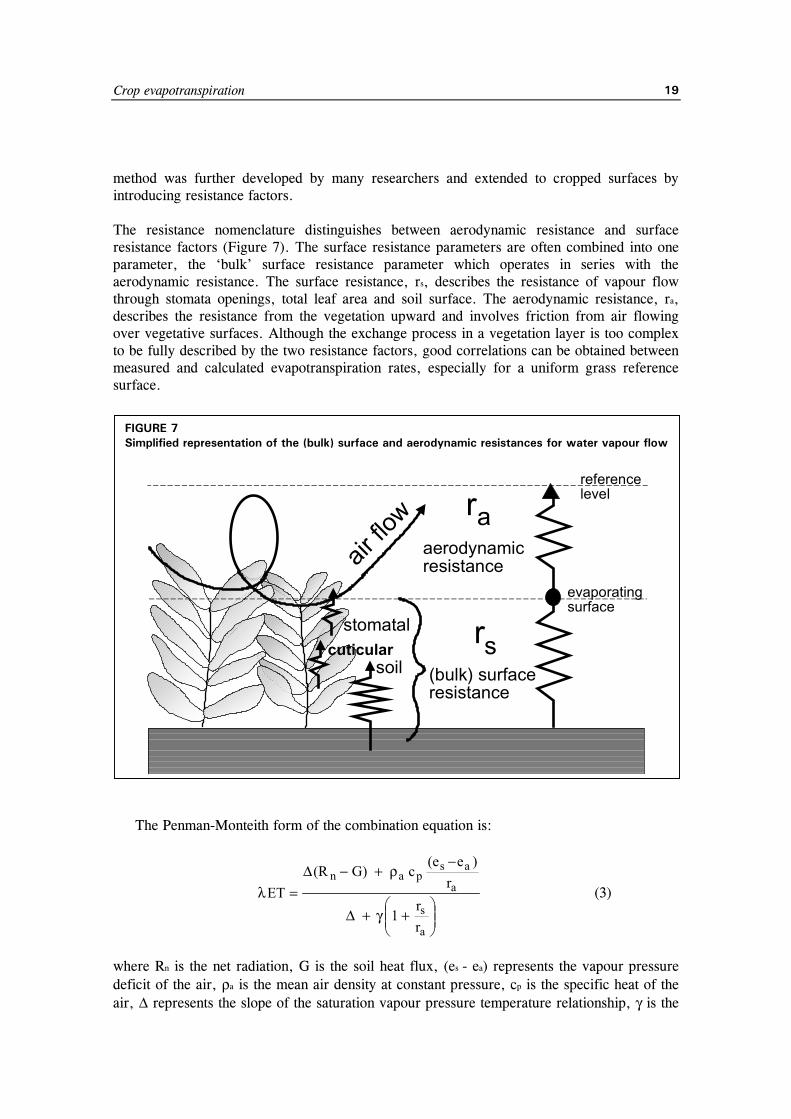
balance above a well-watered transpiring surface on a cloudless day 10 6. Soil water balance of the root zone 12 7. Simplified representation of the (bulk) surface and aerodynamic resistances for
water vapour flow 19 8. Typical presentation of the variation in the green Leaf Area Index over the
growing season for a maize crop 22 9. Characteristics of the hypothetical reference crop 24 10. Illustration of the effect of wind speed on evapotranspiration in hot-dry and humid-
warm weather conditions 30 11. Saturation vapour pressure shown as a function of temperature: e°(T) curve 34 12. Variation of the relative humidity over 24 hours for a constant actual vapour
pressure of 2.4 kPa 34 13. Annual variation in extraterrestrial radiation (Ra) at the equator, 20 and 40° north
and south 41 14. Annual variation of the daylight hours (N) at the equator, 20 and 40° north and
south 42 15. Various components of radiation 44 16. Conversion factor to convert wind speed measured at a certain height above
ground level to wind speed at the standard height (2 m) 56 17. Relationship between the fraction of extraterrestrial radiation that reaches the
earth's surface, Rs/Ra, and the air temperature difference Tmax - Tmin for interior (kRs = 0.16) and coastal (kRs = 0.19) regions 61
18. ETo computed by CROPWAT 69 19. Two cases of evaporation pan siting and their environment 79 20. Typical Kc for different types of full grown crops 92 21. Extreme ranges expected in Kc for full grown crops as climate and weather change 92 22. The effect of evaporation on Kc. The horizontal line represents Kc when the soil
surface is kept continuously wet. The curved line corresponds to Kc when the soil surface is kept dry but the crop receives sufficient water to sustain full transpiration 94
23. Crop growth stages for different types of crops 94
Crop evapotranspiration
xiii
Page 24. Typical ranges expected in Kc for the four growth stages 97 25. Generalized crop coefficient curve for the single crop coefficient approach 100 26. Crop coefficient curves showing the basal Kcb (thick line), soil evaporation Ke)
(thin line) and the corresponding single Kc = Kcb + Ke curve (dashed line) 100 27. General procedure for calculating ETc 102 28. Variation in the length of the growing period of rice (cultivar: Jaya) sown during
various months of the year at different locations along the Senegal River (Africa) 109 29. Average Kc ini as related to the level of ETo and the interval between irrigations
and/or significant rain during the initial growth stage for all soil types when wetting events are light (about 10 mm per event) 117
30. Average Kc ini as related to the level of ETo and the interval between irrigations greater than or equal to 40 mm per wetting event, during the initial growth stage for: a) coarse textured soils; b) medium and fine textured soils 118
31. Partial wetting by irrigation120 32. Adjustment (additive) to the Kc mid values from Table 12 for different crop
heights and mean daily wind speeds (u2) for different humidity conditions 122 33. Ranges expected for Kc end 126 34. Crop coefficient curve 126 35. Constructed curve for Kc for alfalfa hay in southern Idaho, the United States using
values from Tables 11 and 12 and adjusted using Equations 62 and 65 128 36. Kc curve and ten-day values for Kc and ETc derived from the graph for the dry
bean crop example (Box 15) 132 37. Constructed basal crop coefficient (Kcb) curve for a dry bean crop (Example 28)
using growth stage lengths of 25, 25, 30 and 20 days 142 38. Soil evaporation reduction coefficient, Kr 145 39. Determination of variable few as a function of the fraction of ground surface
coverage (fc) and the fraction of the surface wetted (fw) 148 40. Water balance of the topsoil layer 152 41. Depletion factor for different levels of crop evapotranspiration 166 42. Water stress coefficient, Ks 167 43. Water balance of the root zone 169 44. The effect of soil salinity on the water stress coefficient Ks 181 45. Different situations of intercropping 198 46. Kc curves for small areas of vegetation under the oasis effect as a function of the
width of the expanse of vegetation for conditions where RHmin = 30%, u2 = 2 m/s, vegetation height (h) = 2 m and LAI = 3 203
47. Mean evapotranspiration during non-growing, winter periods at Kimberly, Idaho, measured using precision weighing lysimeters 210

xiv
List of tables Page 1. Conversion factors for evapotranspiration 4 2. Average ETo for different agroclimatic regions in mm/day 8 3. Conversion factors for radiation 45 4. General classes of monthly wind speed data 63 5. Pan coefficients (Kp) for Class A pan for different pan siting and environment and
different levels of mean relative humidity and wind speed 81 6. Pan coefficients (Kp) for Colorado sunken pan for different pan siting and
environment and different levels of mean relative humidity and wind speed 81 7. Pan coefficients (Kp): regression equations derived from Tables 5 and 6 82 8. Ratios between the evaporation from sunken pans and a Colorado sunken pan for
different climatic conditions and environments 83 9. Approximate values for Kc ini for medium wetting events (10-40 mm) and a
medium textured soil 95 10. General selection criteria for the single and dual crop coefficient approaches 98 11. Lengths of crop development stages for various planting periods and climatic
regions 104 12. Single (time-averaged crop coefficients) Kc and mean maximum plant heights for
non-stressed, well-managed crops in sub-humid climates (RHmin ≈ 45%, u2 ≈ 2 m/s) for use with the FAO Penman-Monteith ETo 110
13. Classification of rainfall depths 115 14. Kc ini for rice for various climatic conditions 121 15. Empirical estimates of monthly wind speed data 124 16. Typical values for RHmin compared with RHmean for general climatic
classifications 124 17. Basal crop coefficient Kcb for non-stressed, well-managed crops in sub-humid
climates (RHmin ≈ 45%, u2 ≈ 2 m/s) for use with the FAO Penman-Monteith ETo 137
18. General guidelines to derive Kcb from the Kc values listed in Table 12 141 19. Typical soil water characteristics for different soil types 144 20. Common values of fraction fw of soil surface wetted by irrigation or precipitation 149 21. Common values of fractions covered by vegetation (fc) and exposed to sunlight (1-
fc) 149 22. Ranges of maximum effective rooting depth (Zr), and soil water depletion fraction
for no stress (p), for common crops 163 23. Salt tolerance of common agricultural crops as a function of the electrical
conductivity of the soil saturation extract at the threshold when crop yield first reduces below the full yield potential (ECe, threshold) and when crop yields becomes zero (ECe, no yield). source: FAO Irrigation and Drainage Paper No. 33 178
24. Seasonal yield response functions from FAO Irrigation and Drainage Paper No. 33 181 25. Approximate reductions in Kc and surface evaporation, and increases in
transpiration for various horticultural crops under plastic mulch as compared with no mulch using trickle irrigation 196
Crop evapotranspiration
xv
List of boxes
1. Chapters concerning the calculation of the reference crop evapotranspiration (ETo) 8
2. Chapters concerning the calculation of crop evapotranspiration under standard conditions (ETc) 8
3. Chapters concerning the calculation of crop evapotranspiration under non-standard conditions (ETc adj) 10
4. The aerodynamic resistance for a grass reference surface 21
5. The (bulk) surface resistance for a grass reference crop 22
6. Derivation of the FAO Penman-Monteith equation for the hypothetical grass reference crop 26
7. Calculation sheet for vapour pressure deficit (es - ea) 40
8. Conversion from energy values to equivalent evaporation 44
9. Calculation sheet for extraterrestrial radiation (Ra) and daylight hours (N) 49
10. Calculation sheet for net radiation (Rn) 53
11. Calculation sheet for ETo (FAO Penman-Monteith equation) 67
12. Description of Class A pan 84
13. Description of Colorado sunken pan 85
14. Demonstration of effect of climate on Kc mid for tomato crop grown in field 123
15. Case study of a dry bean crop at Kimberly, Idaho, the United States (single crop coefficient) 130
16. Case study of dry bean crop at Kimberly, Idaho, the United States (dual crop coefficient) 158
17. Measuring and estimating LAI 186
18. Measuring and estimating fc eff 187
xvi
List of examples Page 1. Converting evaporation from one unit to another 4 2. Determination of atmospheric parameters 32 3. Determination of saturation vapour pressure 36 4. Determination of actual vapour pressure from psychrometric readings 38 5. Determination of actual vapour pressure from relative humidity 39 6. Determination of vapour pressure deficit 39 7. Conversion of latitude in degrees and minutes to radians 46 8. Determination of extraterrestrial radiation 47 9. Determination of daylight hours 49 10. Determination of solar radiation from measured duration of sunshine 50 11. Determination of net longwave radiation 52 12. Determination of net radiation 53 13. Determination of soil heat flux for monthly periods 55 14. Adjusting wind speed data to standard height 56 15. Determination of solar radiation from temperature data 61 16. Determination of net radiation in the absence of radiation data 62 17. Determination of ETo with mean monthly data 70 18. Determination of ETo with daily data 72 19. Determination of ETo with hourly data 75 20. Determination of ETo with missing data 77 21. Determination of ETo from pan evaporation using tables 83 22. Determination of ETo from pan evaporation using equations 86 23. Estimation of interval between wetting events 116 24. Graphical determination of Kc ini 116 25. Interpolation between light and heavy wetting events 119 26. Determination of Kc ini for partial wetting of the soil surface 120 27. Determination of Kc mid 125 28. Numerical determination of Kc 133 29. Selection and adjustment of basal crop coefficients, Kcb 136 30. Determination of daily values for Kcb 141
Crop evapotranspiration
xvii
Page 31. Determination of the evapotranspiration from a bare soil 146 32. Calculation of the crop coefficient (Kcb + Ke) under sprinkler irrigation 150 33. Calculation of the crop coefficient (Kcb + Ke) under furrow irrigation 151 34. Calculation of the crop coefficient (Kcb + Ke) under drip irrigation 151 35. Estimation of crop evapotranspiration with the dual crop coefficient approach 154 36. Determination of readily available soil water for various crops and soil types 166 37. Effect of water stress on crop evapotranspiration 168 38. Irrigation scheduling to avoid crop water stress 172 39. Effect of soil salinity on crop evapotranspiration 182 40. First approximation of the crop coefficient for the mid-season stage for sparse
vegetation 185 41. Estimation of mid-season crop coefficient 190 42. Estimation of mid-season crop coefficient for reduced ground cover 191 43. Estimation of Kcb mid from ground cover with reduction for stomatal control 192 44. approximate estimation of Ks from crop yield data 194 45. Effects of surface mulch 197 46. Intercropped maize and beans 200 47. Overlapping vegetation 201
xviii
List of equations Page 1. Energy balance equation 11 2. Soil water balance 12 3. Penman-Monteith form of the combination equation 19 4. Aerodynamic resistance (ra) 20 5. (Bulk) surface resistance (rs) 21 6. FAO Penman-Monteith equation for daily, ten-day and monthly time steps 24 7. Atmospheric pressure (P) 31 8. Psychrometric constant (γ) 32 9. Mean air temperature (Tmean) 33 10. Relative humidity (RH) 35 11. Saturation vapour pressure as a function of temperature (e°(T)) 36 12. Saturation vapour pressure (es) 36 13. Slope e°(T) curve (∆) 37 14. Actual vapour pressure derived from dewpoint temperature (ea) 37 15. Actual vapour pressure derived from psychrometric data (ea) 37 16. Psychrometric constant of the (psychrometric) instrument (γpsy) 37 17. Actual vapour pressure derived from RHmax and RHmin (ea) 38 18. Actual vapour pressure derived from RHmax (ea) 39 19. Actual vapour pressure derived from RHmean (ea) 39 20. Conversion form energy to equivalent evaporation 44 21. Extraterrestrial radiation for daily periods (Ra) 46 22. Conversion from decimal degrees to radians 46 23. Inverse relative distance Earth-Sun (dr) 46 24. Solar declination (δ) 46 25. Sunset hour angle - arccos function (ωs) 46 26. Sunset hour angle - arctan function (ωs) 47 27. Parameter X of Equation 26 47 28. Extraterrestrial radiation for hourly or shorter periods (Ra) 47 29. Solar time angle at the beginning of the period (ω1) 48
Crop evapotranspiration
xix
Page
30. Solar time angle at the end of the period (ω2) 48
31. Solar time angle at midpoint of the period (ω) 48
32. Seasonal correction for solar time (Sc) 48
33. Parameter b of Equation 32 48
34. Daylight hours (N) 48
35. Solar radiation (Rs) 50
36. Clear-sky radiation near sea level (Rso) 51
37. Clear-sky radiation at higher elevations (Rso) 51
38. Net solar or net shortwave radiation (Rns) 51
39. Net longwave radiation (Rnl) 52
40. Net radiation (Rn) 53
41. Soil heat flux (G) 54
42. Soil heat flux for day and ten-day periods (Gday) 54
43. Soil heat flux for monthly periods (Gmonth) 54
44. Soil heat flux for monthly periods if Tmonth,i+1 is unknown (Gmonth) 54
45. Soil heat flux for hourly or shorter periods during daytime (Ghr) 55
46. Soil heat flux for hourly or shorter periods during nighttime (Ghr) 55
47. Adjustment of wind speed to standard height (u2) 56
48. Estimating actual vapour pressure from Tmin (ea) 58
49. Importing solar radiation from a nearby weather station (Rs) 59
50. Estimating solar radiation from temperature differences (Hargreaves’ formula) 60
51. Estimating solar radiation for island locations (Rs) 62
52. 1985 Hargreaves reference evapotranspiration equation 64
53. FAO Penman-Monteith equation for hourly time step 74
54. Actual vapour pressure for hourly time step 74
55. Deriving ETo from pan evaporation 79
56. Crop evapotranspiration (ETc) 90
57. Dual crop coefficient 98
58. Crop evapotranspiration - single crop coefficient (ETc) 103
59. Interpolation for infiltration depths between 10 and 40 mm 117
60. Adjustment of Kc ini for partial wetting by irrigation 119
61. Irrigation depth for the part of the surface that is wetted (Iw) 119
62. Climatic adjustment for Kc mid 121
xx
Page
63. Minimum relative humidity estimated from e°(Tdew) 123
64. Minimum relative humidity estimated from e°(Tmin) 124
65. Climatic adjustment for Kc end 125
66. Interpolation of Kc for crop development stage and late season stage 132
67. Relation between grass-based and alfalfa-based crop coefficients 133
68. Ratio between grass-based and alfalfa-based Kc for Kimberly, Idaho 134
69. Crop evapotranspiration - dual crop coefficient (ETc) 135
70. Climatic adjustment for Kcb 136
71. Soil evaporation coefficient (Ke) 142
72. Upper limit on evaporation and transpiration from any cropped surface (Kc max) 143
73. Maximum depth of water that can be evaporated from the topsoil (TEW) 144
74. Evaporation reduction coefficient (Kr) 146
75. Exposed and wetted soil fraction (few) 147
76. Effective fraction of soil surface that is covered by vegetation (fc) 149
77. Daily soil water balance for the exposed and wetted soil fraction 152
78. Limits on soil water depletion by evaporation (De) 153
79. Drainage out of topsoil (DPe) 156
80. Crop evapotranspiration adjusted for water stress - dual crop coefficient 161
81. Crop evapotranspiration adjusted for water stress - single crop coefficient 161
82. Total available soil water in the root zone (TAW) 162
83. Readily available soil water in the root zone (RAW) 162
84. Water stress coefficient (Ks) 169
85. Water balance of the root zone 170
86. Limits on root zone depletion by evapotranspiration (Dr) 170
87. Initial depletion (Dr,i-1) 170
88. Deep percolation (DP) 171
89. Relative crop yield (Ya/Ym) determined from soil salinity (ECe) and crop salinity threshold
90. Yield response to water function (FAO Irrigation and Drainage Paper No. 33) 176
91. Water stress coefficient (Ks) under saline conditions 177
92. Water stress coefficient (Ks) under saline and water stress conditions 177
93. Soil salinity (ECe) predicted from leaching fraction (LF) and irrigation water quality (ECiw) 180
94. Kc adj for reduced plant coverage 184
Crop evapotranspiration
xxi
95. Adjustment coefficient (from LAI) 185
96. Adjustment coefficient (from fc) 185
97. K(cb mid) adj from Leaf Area Index 186
98. K(cb mid) adj from effective ground cover 187
99. Kcb full for agricultural crops 189
100. Kcb full for natural vegetation 189
101. Kcb h for full cover vegetation 189
102. Adjustment for stomatal control (Fr) 191
103. Water stress coefficient (Ks) estimated from yield response to water function 194
104. Crop coefficient estimate for intercropped field (Kc field) 199
105. Crop coefficient estimate for windbreaks (Kc) 203

xxii
List of principal symbols and acronyms apsy coefficient of psychrometer [°C-1]
as fraction of extraterrestrial radiation reaching the earth on an overcast day [-]
as+bs fraction of extraterrestrial radiation reaching the earth on a clear day [-]
cp specific heat [MJ kg-1 °C-1]
cs soil heat capacity [MJ m-3 °C-1]
CR capillary rise [mm day-1]
De cumulative depth of evaporation (depletion) from the soil surface layer [mm]
Dr cumulative depth of evapotranspiration (depletion) from the root zone [mm]
d zero plane displacement height [m]
dr inverse relative distance Earth-Sun [-]
DP deep percolation [mm]
DPe deep percolation from the evaporation layer [mm]
E evaporation [mm day-1]
Epan pan evaporation [mm day-1]
e°(T) saturation vapour pressure at air temperature T [kPa]
es saturation vapour pressure for a given time period [kPa]
ea actual vapour pressure [kPa]
es- ea saturation vapour pressure deficit
ECe electrical conductivity of the saturation extract of the soil [dS m-1]
ECe, threshold electrical conductivity of the saturation extract of the soil above which yield begins to decrease [dS m-1]
ET evapotranspiration [mm day-1]
ETo reference crop evapotranspiration [mm day-1]
ETc crop evapotranspiration under standard conditions [mm day-1]
ETc adj crop evapotranspiration under non-standard conditions [mm day-1]
exp[x] 2.7183 (base of natural logarithm) raised to the power x
Fr resistance correction factor [-]
Crop evapotranspiration
xxiii
fc fraction of soil surface covered by vegetation (as observed from overhead) [-]
fc eff effective fraction of soil surface covered by vegetation [-]
1-fc exposed soil fraction [-]
fw fraction of soil surface wetted by rain or irrigation [-]
few fraction of soil that is both exposed and wetted (from which most evaporation occurs) [-]
G soil heat flux [MJ m-2 day-1]
Gday soil heat flux for day and ten-day periods [MJ m-2 day-1]
Ghr soil heat flux for hourly or shorter periods [MJ m-2 hour-1]
Gmonth soil heat flux for monthly periods [MJ m-2 day-1]
Gsc solar constant [0.0820 MJ m-2 min-1]
H sensible heat [MJ m-2 day-1]
HWR height to width ratio
h crop height [m]
I irrigation depth [mm]
Iw irrigation depth for that part of the surface wetted [mm]
J number of day in the year [-]
Kc crop coefficient [-]
Kc ini crop coefficient during the initial growth stage [-]
Kc mid crop coefficient during the mid-season growth stage [-]
Kc end crop coefficient at end of the late season growth stage [-]
Kc max maximum value of crop coefficient (following rain or irrigation) [-]
Kc min minimum value of crop coefficient (dry soil with no ground cover) [-]
Kcb basal crop coefficient [-]
Kcb full basal crop coefficient during mid-season (at peak plant size or height) for vegetation with full ground cover of LAI > 3 [-]
Kcb ini basal crop coefficient during the initial growth stage [-]
Kcb mid basal crop coefficient during the mid-season growth stage [-]
Kcb end basal crop coefficient at end of the late season growth stage [-]
Ke soil evaporation coefficient [-]
Kp pan coefficient [-]
Kr soil evaporation reduction coefficient [-]
xxiv
Ks water stress coefficient [-]
Ky yield response factor [-]
k von Karman's constant [0.41] [-]
kRs adjustment coefficient for the Hargreaves’ radiation formula [°C-0.5]
Lini length of initial growth stage [day]
Ldev length of crop development growth stage [day]
Lmid length of mid-season growth stage [day]
Llate length of late season growth stage [day]
Lz longitude of centre of local time zone [degrees west of Greenwich]
Lm longitude [degrees west of Greenwich]
LAI leaf area index [m2 (leaf area) m-2 (soil surface)]
LAIactive active (sunlit) leaf area index [-]
N maximum possible sunshine duration in a day, daylight hours [hour]
n actual duration of sunshine in a day [hour]
n/N relative sunshine duration [-]
P rainfall [mm], atmospheric pressure [kPa]
p evapotranspiration depletion factor [-]
R specific gas constant [0.287 kJ kg-1 K-1]
Ra extraterrestrial radiation [MJ m-2 day-1]
Rl longwave radiation [MJ m-2 day-1]
Rn net radiation [MJ m-2 day-1]
Rnl net longwave radiation [MJ m-2 day-1]
Rns net solar or shortwave radiation [MJ m-2 day-1]
Rs solar or shortwave radiation [MJ m-2 day-1]
Rso clear-sky solar or clear-sky shortwave radiation [MJ m-2 day-1]
ra aerodynamic resistance [s m-1]
rl bulk stomatal resistance of well-illuminated leaf [s m-1]
rs (bulk) surface or canopy resistance [s m-1]
Rs/Rso relative solar or relative shortwave radiation [-]
RAW readily available soil water of the root zone [mm]
Crop evapotranspiration
xxv
REW readily evaporable water (i.e., maximum depth of water that can be evaporated from the soil surface layer without restriction during stage 1) [mm]
RH relative humidity [%]
RHhr average hourly relative humidity
RHmax daily maximum relative humidity [%]
RHmean daily mean relative humidity [%]
RHmin daily minimum relative humidity [%]
RO surface runoff [mm]
Sc seasonal correction factor for solar time [hour]
SF subsurface flow [mm]
T air temperature [°C]
TK air temperature [K]
TKv virtual air temperature [K]
Tdew dewpoint temperature [°C]
Tdry temperature of dry bulb [°C]
Tmax daily maximum air temperature [°C]
Tmax,K daily maximum air temperature [K]
Tmean daily mean air temperature [°C]
Tmin daily minimum air temperature [°C]
Tmin,K daily minimum air temperature [K]
Twet temperature of wet bulb [°C]
TAW total available soil water of the root zone [mm]
TEW total evaporable water (i.e., maximum depth of water that can be evaporated from the soil surface layer)[mm]
t time [hour]
u2 wind speed at 2 m above ground surface [m s-1]
uz wind speed at z m above ground surface [m s-1]
W soil water content [mm]
Ya actual yield of the crop [kg ha-1]
Ym maximum (expected) yield of the crop in absence of environment or water stresses [kg ha-1]
Ze depth of surface soil layer subjected to drying by evaporation [m]
xxvi
Zr rooting depth [m]
z elevation, height above sea level [m]
zh height of humidity measurements [m]
zm height of wind measurements [m]
zom roughness length governing momentum transfer [m]
zoh roughness length governing heat and vapour transfer [m]
α albedo [-]
γ psychrometric constant [kPa °C-1]
γpsy psychrometric constant of instrument [kPa °C-1]
∆ slope of saturation vapour pressure curve [kPa °C-1]
∆SW variation in soil water content [mm]
∆t length of time interval [day]
∆z effective soil depth [m]
δ solar declination [rad]
ε ratio molecular weight of water vapour/dry air (= 0.622)
η mean angle of the sun above the horizon
θ soil water content [m3(water) m-3(soil)]
θFC soil water content at field capacity [m3(water) m-3(soil)]
θt threshold soil water content below which transpiration is reduced due to water stress [m3(water) m-3(soil)]
θWP soil water content at wilting point [m3(water) m-3(soil)]
λ latent heat of vaporization [MJ kg-1]
λET latent heat flux [MJ m-2 day-1]
ρa mean air density [kg m-3]
ρw density of water [kg m-3]
σ Stefan-Boltzmann constant [4.903 10-9 MJ K-4 m-2 day-1]
ϕ latitude [rad]
ω solar time angle at midpoint of hourly or shorter period [rad]
ω1 solar time angle at beginning of hourly or shorter period [rad]
ω2 solar time angle at end of hourly or shorter period [rad]
ωs sunset hour angle [rad]
Crop evapotranspiration
1
Chapter 1
Introduction to evapotranspiration This chapter explains the concepts of and the differences between reference crop evapotranspiration (ETo) and crop evapotranspiration under standard conditions (ETc) and various management and environmental conditions (ETc adj). It also examines the factors that affect evapotranspiration, the units in which it is normally expressed and the way in which it can be determined. EVAPOTRANSPIRATION PROCESS
The combination of two separate processes whereby water is lost on the one hand from the soil surface by evaporation and on the other hand from the crop by transpiration is referred to as evapotranspiration (ET). Evaporation
Evaporation is the process whereby liquid water is converted to water vapour (vaporization) and removed from the evaporating surface (vapour removal). Water evaporates from a variety of surfaces, such as lakes, rivers, pavements, soils and wet vegetation. Energy is required to change the state of the molecules of water from liquid to vapour. Direct solar radiation and, to a lesser extent, the ambient temperature of the air provide this energy. The driving force to remove water vapour from the evaporating surface is the difference between the water vapour pressure at the evaporating surface and that of the surrounding atmosphere. As evaporation proceeds, the surrounding air becomes gradually saturated and the process will slow down and might stop if the wet air is not transferred to the atmosphere. The replacement of the saturated air with drier air depends greatly on wind speed. Hence, solar radiation, air temperature, air humidity and wind speed are climatological parameters to consider when assessing the evaporation process.
Where the evaporating surface is the soil surface, the degree of shading of the crop canopy and the amount of water available at the evaporating surface are other factors that affect the evaporation process. Frequent rains, irrigation and water transported upwards in a soil from a shallow water table wet the soil surface. Where the soil is able to supply water fast enough to satisfy the evaporation demand, the evaporation from the soil is determined only by the meteorological conditions. However, where the interval between rains and irrigation becomes large and the ability of the soil to conduct moisture to near the surface is small, the water content in the topsoil drops and the soil surface dries out. Under these circumstances the limited availability of water exerts a controlling influence on soil evaporation. In the absence of any supply of water to the soil surface, evaporation decreases rapidly and may cease almost completely within a few days.
Introduction to evapotranspiration
2
FIGURE 1 Schematic representation of a stoma
water vapour
cuticula
epidermalcells
mesophyllcells
intercellularspace
Atmosphere
water
LeafFIGURE 2 The partitioning of evapotranspiration into evaporation and transpiration over the growing periodfor an annual field crop
0%
20%
40%
60%
80%
100%
time
part
ition
ing
of e
vapo
tran
spira
tion
leaf
are
a in
dex
(LA
I)
evaporation
transpiration
sowing harvest
crop
soil
L A I
Crop evapotranspiration
3
Transpiration
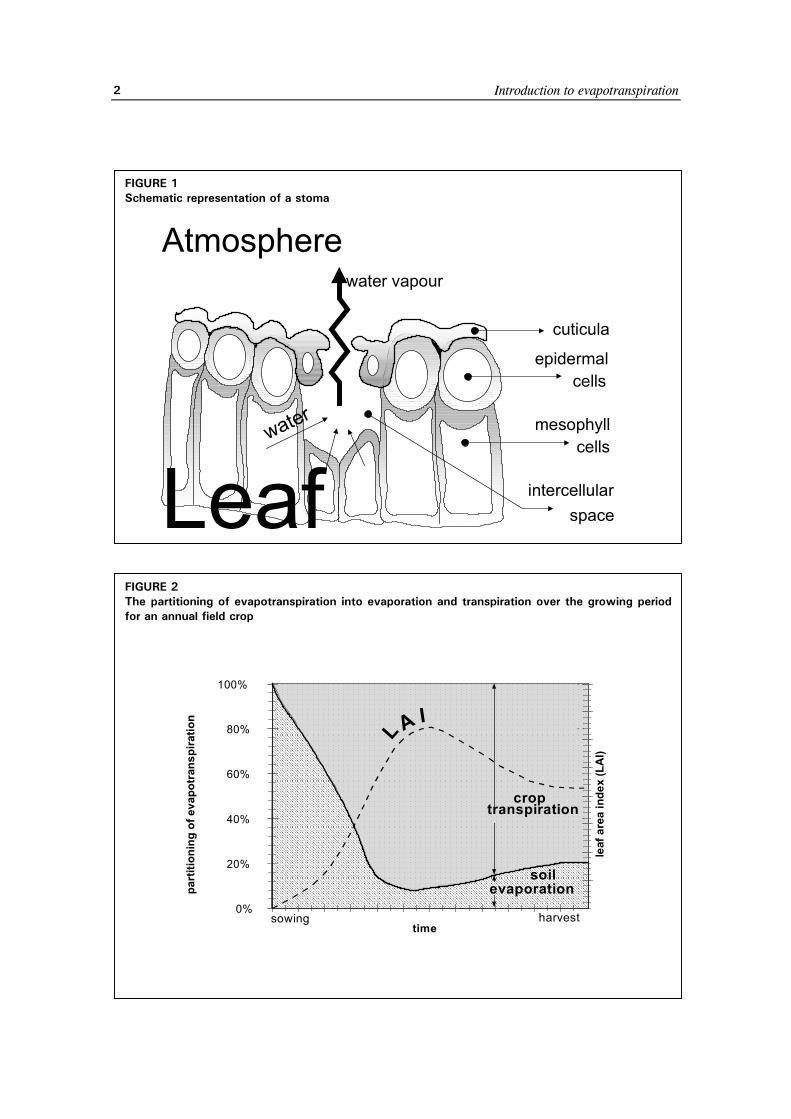
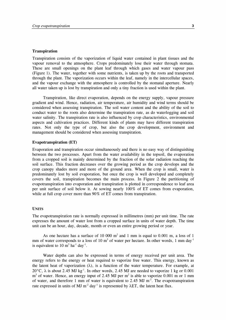
Transpiration consists of the vaporization of liquid water contained in plant tissues and the vapour removal to the atmosphere. Crops predominately lose their water through stomata. These are small openings on the plant leaf through which gases and water vapour pass (Figure 1). The water, together with some nutrients, is taken up by the roots and transported through the plant. The vaporization occurs within the leaf, namely in the intercellular spaces, and the vapour exchange with the atmosphere is controlled by the stomatal aperture. Nearly all water taken up is lost by transpiration and only a tiny fraction is used within the plant.
Transpiration, like direct evaporation, depends on the energy supply, vapour pressure gradient and wind. Hence, radiation, air temperature, air humidity and wind terms should be considered when assessing transpiration. The soil water content and the ability of the soil to conduct water to the roots also determine the transpiration rate, as do waterlogging and soil water salinity. The transpiration rate is also influenced by crop characteristics, environmental aspects and cultivation practices. Different kinds of plants may have different transpiration rates. Not only the type of crop, but also the crop development, environment and management should be considered when assessing transpiration. Evapotranspiration (ET)
Evaporation and transpiration occur simultaneously and there is no easy way of distinguishing between the two processes. Apart from the water availability in the topsoil, the evaporation from a cropped soil is mainly determined by the fraction of the solar radiation reaching the soil surface. This fraction decreases over the growing period as the crop develops and the crop canopy shades more and more of the ground area. When the crop is small, water is predominately lost by soil evaporation, but once the crop is well developed and completely covers the soil, transpiration becomes the main process. In Figure 2 the partitioning of evapotranspiration into evaporation and transpiration is plotted in correspondence to leaf area per unit surface of soil below it. At sowing nearly 100% of ET comes from evaporation, while at full crop cover more than 90% of ET comes from transpiration. UNITS
The evapotranspiration rate is normally expressed in millimetres (mm) per unit time. The rate expresses the amount of water lost from a cropped surface in units of water depth. The time unit can be an hour, day, decade, month or even an entire growing period or year.
As one hectare has a surface of 10 000 m2 and 1 mm is equal to 0.001 m, a loss of 1 mm of water corresponds to a loss of 10 m3 of water per hectare. In other words, 1 mm day-1 is equivalent to 10 m3 ha-1 day-1.
Water depths can also be expressed in terms of energy received per unit area. The energy refers to the energy or heat required to vaporize free water. This energy, known as the latent heat of vaporization (λ), is a function of the water temperature. For example, at 20°C, λ is about 2.45 MJ kg-1. In other words, 2.45 MJ are needed to vaporize 1 kg or 0.001 m3 of water. Hence, an energy input of 2.45 MJ per m2 is able to vaporize 0.001 m or 1 mm of water, and therefore 1 mm of water is equivalent to 2.45 MJ m-2. The evapotranspiration rate expressed in units of MJ m-2 day-1 is represented by λET, the latent heat flux.
Introduction to evapotranspiration
4
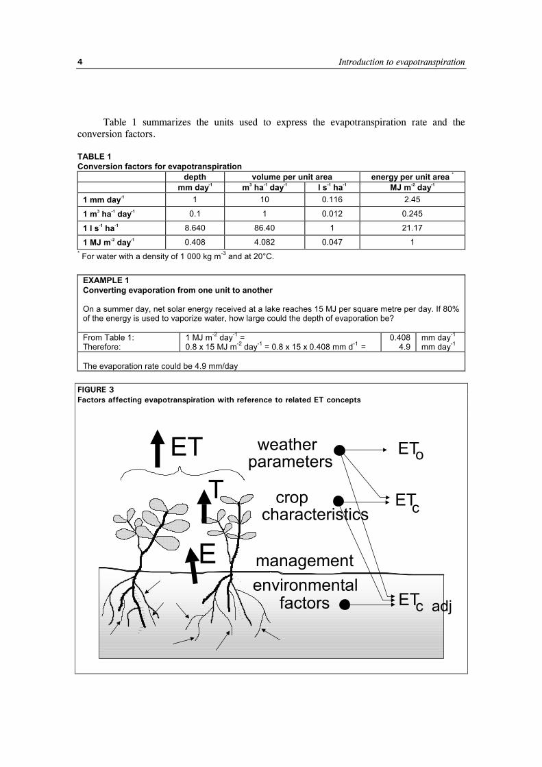
Table 1 summarizes the units used to express the evapotranspiration rate and the conversion factors. TABLE 1 Conversion factors for evapotranspiration
depth volume per unit area energy per unit area * mm day-1 m3 ha-1 day-1 l s-1 ha-1 MJ m-2 day-1 1 mm day-1 1 10 0.116 2.45
1 m3 ha-1 day-1 0.1 1 0.012 0.245
1 l s-1 ha-1 8.640 86.40 1 21.17
1 MJ m-2 day-1 0.408 4.082 0.047 1 * For water with a density of 1 000 kg m-3 and at 20°C.
EXAMPLE 1 Converting evaporation from one unit to another On a summer day, net solar energy received at a lake reaches 15 MJ per square metre per day. If 80% of the energy is used to vaporize water, how large could the depth of evaporation be? From Table 1: Therefore:
1 MJ m-2 day-1 = 0.8 x 15 MJ m-2 day-1 = 0.8 x 15 x 0.408 mm d-1 =
0.408 4.9
mm day-1 mm day-1
The evaporation rate could be 4.9 mm/day
FIGURE 3 Factors affecting evapotranspiration with reference to related ET concepts
cropcharacteristics
weatherparameters
ETT
E
ETo
ETc
ETenvironmental
factors
management
c adj
Crop evapotranspiration
5
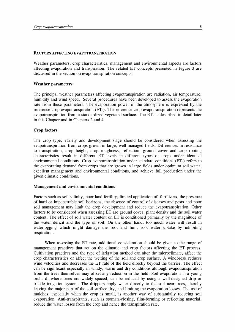
FACTORS AFFECTING EVAPOTRANSPIRATION Weather parameters, crop characteristics, management and environmental aspects are factors affecting evaporation and transpiration. The related ET concepts presented in Figure 3 are discussed in the section on evapotranspiration concepts. Weather parameters The principal weather parameters affecting evapotranspiration are radiation, air temperature, humidity and wind speed. Several procedures have been developed to assess the evaporation rate from these parameters. The evaporation power of the atmosphere is expressed by the reference crop evapotranspiration (ETo). The reference crop evapotranspiration represents the evapotranspiration from a standardized vegetated surface. The ETo is described in detail later in this Chapter and in Chapters 2 and 4. Crop factors The crop type, variety and development stage should be considered when assessing the evapotranspiration from crops grown in large, well-managed fields. Differences in resistance to transpiration, crop height, crop roughness, reflection, ground cover and crop rooting characteristics result in different ET levels in different types of crops under identical environmental conditions. Crop evapotranspiration under standard conditions (ETc) refers to the evaporating demand from crops that are grown in large fields under optimum soil water, excellent management and environmental conditions, and achieve full production under the given climatic conditions. Management and environmental conditions Factors such as soil salinity, poor land fertility, limited application of fertilizers, the presence of hard or impenetrable soil horizons, the absence of control of diseases and pests and poor soil management may limit the crop development and reduce the evapotranspiration. Other factors to be considered when assessing ET are ground cover, plant density and the soil water content. The effect of soil water content on ET is conditioned primarily by the magnitude of the water deficit and the type of soil. On the other hand, too much water will result in waterlogging which might damage the root and limit root water uptake by inhibiting respiration.
When assessing the ET rate, additional consideration should be given to the range of management practices that act on the climatic and crop factors affecting the ET process. Cultivation practices and the type of irrigation method can alter the microclimate, affect the crop characteristics or affect the wetting of the soil and crop surface. A windbreak reduces wind velocities and decreases the ET rate of the field directly beyond the barrier. The effect can be significant especially in windy, warm and dry conditions although evapotranspiration from the trees themselves may offset any reduction in the field. Soil evaporation in a young orchard, where trees are widely spaced, can be reduced by using a well-designed drip or trickle irrigation system. The drippers apply water directly to the soil near trees, thereby leaving the major part of the soil surface dry, and limiting the evaporation losses. The use of mulches, especially when the crop is small, is another way of substantially reducing soil evaporation. Anti-transpirants, such as stomata-closing, film-forming or reflecting material, reduce the water losses from the crop and hence the transpiration rate.
Introduction to evapotranspiration
6
FIGURE 4 Reference (ETo), crop evapotranspiration under standard (ETc) and non-standard conditions (ETc adj)
x =ET
ETKK
water & environmentalstress
s c adjusted c adj
o
x
RadiationTemperatureWind speedHumidity
climate
+ =
x =
well watered
well watered
grassreference
cropETo
ETo
ETcKc factor
grass
cropconditionsoptimal agronomic
Crop evapotranspiration
7
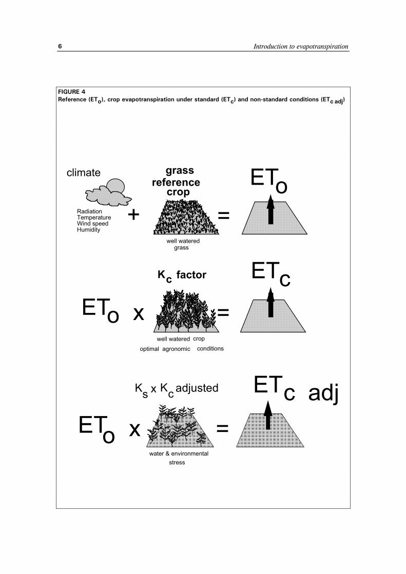
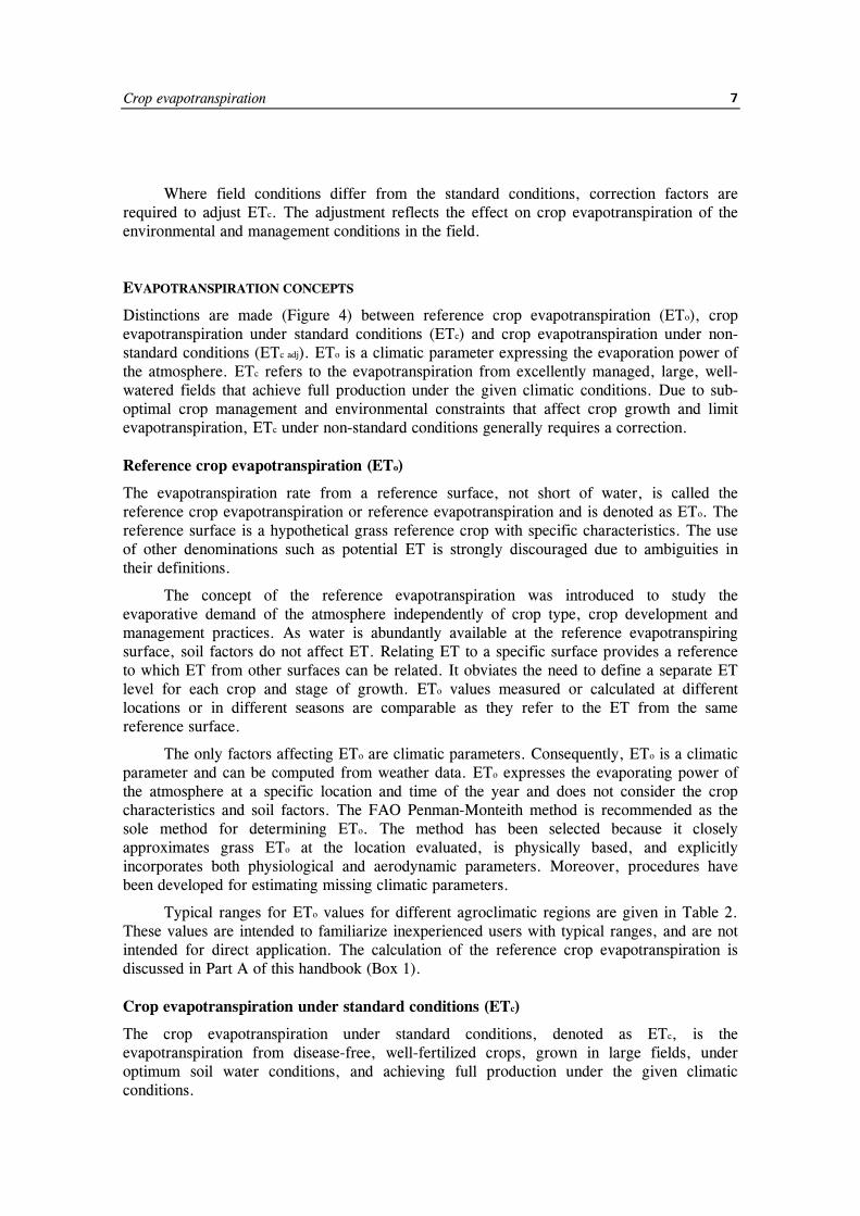
Where field conditions differ from the standard conditions, correction factors are required to adjust ETc. The adjustment reflects the effect on crop evapotranspiration of the environmental and management conditions in the field. EVAPOTRANSPIRATION CONCEPTS
Distinctions are made (Figure 4) between reference crop evapotranspiration (ETo), crop evapotranspiration under standard conditions (ETc) and crop evapotranspiration under non-standard conditions (ETc adj). ETo is a climatic parameter expressing the evaporation power of the atmosphere. ETc refers to the evapotranspiration from excellently managed, large, well-watered fields that achieve full production under the given climatic conditions. Due to sub-optimal crop management and environmental constraints that affect crop growth and limit evapotranspiration, ETc under non-standard conditions generally requires a correction. Reference crop evapotranspiration (ETo)
The evapotranspiration rate from a reference surface, not short of water, is called the reference crop evapotranspiration or reference evapotranspiration and is denoted as ETo. The reference surface is a hypothetical grass reference crop with specific characteristics. The use of other denominations such as potential ET is strongly discouraged due to ambiguities in their definitions.
The concept of the reference evapotranspiration was introduced to study the evaporative demand of the atmosphere independently of crop type, crop development and management practices. As water is abundantly available at the reference evapotranspiring surface, soil factors do not affect ET. Relating ET to a specific surface provides a reference to which ET from other surfaces can be related. It obviates the need to define a separate ET level for each crop and stage of growth. ETo values measured or calculated at different locations or in different seasons are comparable as they refer to the ET from the same reference surface.
The only factors affecting ETo are climatic parameters. Consequently, ETo is a climatic parameter and can be computed from weather data. ETo expresses the evaporating power of the atmosphere at a specific location and time of the year and does not consider the crop characteristics and soil factors. The FAO Penman-Monteith method is recommended as the sole method for determining ETo. The method has been selected because it closely approximates grass ETo at the location evaluated, is physically based, and explicitly incorporates both physiological and aerodynamic parameters. Moreover, procedures have been developed for estimating missing climatic parameters.
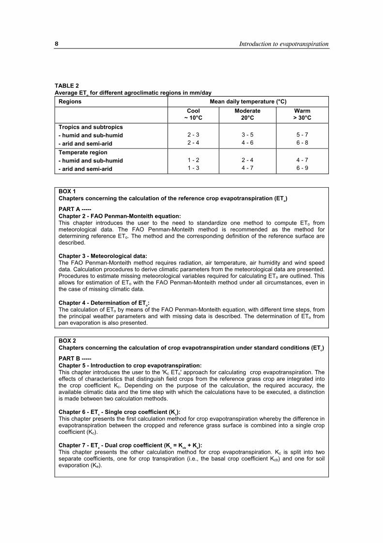
Typical ranges for ETo values for different agroclimatic regions are given in Table 2. These values are intended to familiarize inexperienced users with typical ranges, and are not intended for direct application. The calculation of the reference crop evapotranspiration is discussed in Part A of this handbook (Box 1). Crop evapotranspiration under standard conditions (ETc)
The crop evapotranspiration under standard conditions, denoted as ETc, is the evapotranspiration from disease-free, well-fertilized crops, grown in large fields, under optimum soil water conditions, and achieving full production under the given climatic conditions.
Introduction to evapotranspiration
8
TABLE 2 Average ETo for different agroclimatic regions in mm/day
Regions Mean daily temperature (°C) Cool
~ 10°C Moderate
20°C Warm > 30°C
Tropics and subtropics - humid and sub-humid - arid and semi-arid
2 - 3 2 - 4
3 - 5 4 - 6
5 - 7 6 - 8
Temperate region - humid and sub-humid - arid and semi-arid
1 - 2 1 - 3
2 - 4 4 - 7
4 - 7 6 - 9
BOX 1 Chapters concerning the calculation of the reference crop evapotranspiration (ETo) PART A ----- Chapter 2 - FAO Penman-Monteith equation: This chapter introduces the user to the need to standardize one method to compute ETo from meteorological data. The FAO Penman-Monteith method is recommended as the method for determining reference ETo. The method and the corresponding definition of the reference surface are described. Chapter 3 - Meteorological data: The FAO Penman-Monteith method requires radiation, air temperature, air humidity and wind speed data. Calculation procedures to derive climatic parameters from the meteorological data are presented. Procedures to estimate missing meteorological variables required for calculating ETo are outlined. This allows for estimation of ETo with the FAO Penman-Monteith method under all circumstances, even in the case of missing climatic data. Chapter 4 - Determination of ETo: The calculation of ETo by means of the FAO Penman-Monteith equation, with different time steps, from the principal weather parameters and with missing data is described. The determination of ETo from pan evaporation is also presented.
BOX 2 Chapters concerning the calculation of crop evapotranspiration under standard conditions (ETc) PART B ----- Chapter 5 - Introduction to crop evapotranspiration: This chapter introduces the user to the 'Kc ETo' approach for calculating crop evapotranspiration. The effects of characteristics that distinguish field crops from the reference grass crop are integrated into the crop coefficient Kc. Depending on the purpose of the calculation, the required accuracy, the available climatic data and the time step with which the calculations have to be executed, a distinction is made between two calculation methods. Chapter 6 - ETc - Single crop coefficient (Kc): This chapter presents the first calculation method for crop evapotranspiration whereby the difference in evapotranspiration between the cropped and reference grass surface is combined into a single crop coefficient (Kc). Chapter 7 - ETc - Dual crop coefficient (Kc = Kcb + Ke): This chapter presents the other calculation method for crop evapotranspiration. Kc is split into two separate coefficients, one for crop transpiration (i.e., the basal crop coefficient Kcb) and one for soil evaporation (Ke).
Crop evapotranspiration
9
The amount of water required to compensate the evapotranspiration loss from the cropped field is defined as crop water requirement. Although the values for crop evapotranspiration and crop water requirement are identical, crop water requirement refers to the amount of water that needs to be supplied, while crop evapotranspiration refers to the amount of water that is lost through evapotranspiration. The irrigation water requirement basically represents the difference between the crop water requirement and effective precipitation. The irrigation water requirement also includes additional water for leaching of salts and to compensate for non-uniformity of water application. Calculation of the irrigation water requirement is not covered in this publication, but will be the topic of a future Irrigation and Drainage Paper.
Crop evapotranspiration can be calculated from climatic data and by integrating directly the crop resistance, albedo and air resistance factors in the Penman-Monteith approach. As there is still a considerable lack of information for different crops, the Penman-Monteith method is used for the estimation of the standard reference crop to determine its evapotranspiration rate, i.e., ETo. Experimentally determined ratios of ETc/ETo, called crop coefficients (Kc), are used to relate ETc to ETo or ETc = Kc ETo.
Differences in leaf anatomy, stomatal characteristics, aerodynamic properties and even albedo cause the crop evapotranspiration to differ from the reference crop evapotranspiration under the same climatic conditions. Due to variations in the crop characteristics throughout its growing season, Kc for a given crop changes from sowing till harvest. The calculation of crop evapotranspiration under standard conditions (ETc) is discussed in Part B of this handbook (Box 2). Crop evapotranspiration under non-standard conditions (ETc adj)
The crop evapotranspiration under non-standard conditions (ETc adj) is the evapotranspiration from crops grown under management and environmental conditions that differ from the standard conditions. When cultivating crops in fields, the real crop evapotranspiration may deviate from ETc due to non-optimal conditions such as the presence of pests and diseases, soil salinity, low soil fertility, water shortage or waterlogging. This may result in scanty plant growth, low plant density and may reduce the evapotranspiration rate below ETc.
The crop evapotranspiration under non-standard conditions is calculated by using a water stress coefficient Ks and/or by adjusting Kc for all kinds of other stresses and environmental constraints on crop evapotranspiration. The adjustment to ETc for water stress, management and environmental constraints is discussed in Part C of this handbook (Box 3). DETERMINING EVAPOTRANSPIRATION
ET measurement
Evapotranspiration is not easy to measure. Specific devices and accurate measurements of various physical parameters or the soil water balance in lysimeters are required to determine evapotranspiration. The methods are often expensive, demanding in terms of accuracy of measurement and can only be fully exploited by well-trained research personnel. Although the methods are inappropriate for routine measurements, they remain important for the evaluation of ET estimates obtained by more indirect methods.
Introduction to evapotranspiration
10
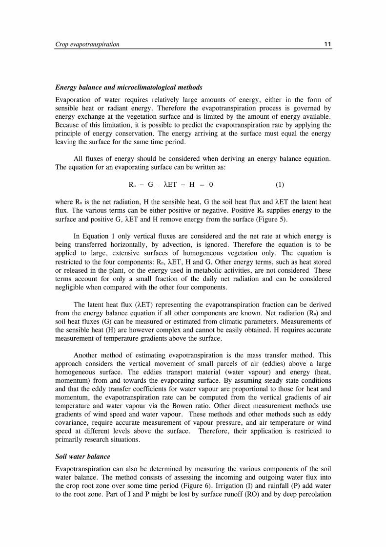
BOX 3 Chapters concerning the calculation of crop evapotranspiration under non-standard conditions (ETc adj) PART C ----- Chapter 8 - ETc under soil water stress conditions: This chapter discusses the reduction in transpiration induced by soil moisture stress or soil water salinity. The resulting evapotranspiration will deviate from the crop evapotranspiration under standard conditions. The evapotranspiration is computed by using a water stress coefficient, Ks, describing the effect of water stress on crop transpiration. Chapter 9 - ETc for natural, non-typical and non-pristine vegetation: Procedures that can be used to make adjustments to the Kc to account for less than perfect growing conditions or stand characteristics are discussed. The procedures can also be used to determine Kc for agricultural crops not listed in the tables of Part B. Chapter 10 - ETc under various management practices: This chapter discusses various types of management practices that may cause the values for Kc and ETc to deviate from the standard conditions described in Part B. Adjustment procedures for Kc to account for surface mulches, intercropping, small areas of vegetation and management induced stress are presented. Chapter 11 - ETc during non-growing periods: This chapter describes procedures for predicting ETc during non-growing periods under various types of surface conditions.
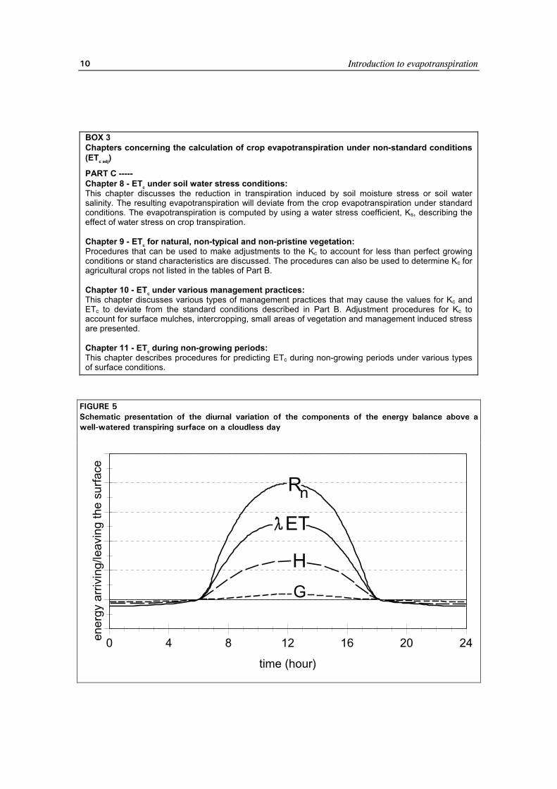
FIGURE 5 Schematic presentation of the diurnal variation of the components of the energy balance above a well-watered transpiring surface on a cloudless day
0 4 8 12 16 20 24
time (hour)
ener
gy a
rrivi
ng/le
avin
g th
e su
rface
Rn
ET
HG
Crop evapotranspiration
11
Energy balance and microclimatological methods
Evaporation of water requires relatively large amounts of energy, either in the form of sensible heat or radiant energy. Therefore the evapotranspiration process is governed by energy exchange at the vegetation surface and is limited by the amount of energy available. Because of this limitation, it is possible to predict the evapotranspiration rate by applying the principle of energy conservation. The energy arriving at the surface must equal the energy leaving the surface for the same time period.
All fluxes of energy should be considered when deriving an energy balance equation. The equation for an evaporating surface can be written as: Rn − G - λET − H = 0 (1) where Rn is the net radiation, H the sensible heat, G the soil heat flux and λET the latent heat flux. The various terms can be either positive or negative. Positive Rn supplies energy to the surface and positive G, λET and H remove energy from the surface (Figure 5).
In Equation 1 only vertical fluxes are considered and the net rate at which energy is being transferred horizontally, by advection, is ignored. Therefore the equation is to be applied to large, extensive surfaces of homogeneous vegetation only. The equation is restricted to the four components: Rn, λET, H and G. Other energy terms, such as heat stored or released in the plant, or the energy used in metabolic activities, are not considered These terms account for only a small fraction of the daily net radiation and can be considered negligible when compared with the other four components.
The latent heat flux (λET) representing the evapotranspiration fraction can be derived from the energy balance equation if all other components are known. Net radiation (Rn) and soil heat fluxes (G) can be measured or estimated from climatic parameters. Measurements of the sensible heat (H) are however complex and cannot be easily obtained. H requires accurate measurement of temperature gradients above the surface.
Another method of estimating evapotranspiration is the mass transfer method. This approach considers the vertical movement of small parcels of air (eddies) above a large homogeneous surface. The eddies transport material (water vapour) and energy (heat, momentum) from and towards the evaporating surface. By assuming steady state conditions and that the eddy transfer coefficients for water vapour are proportional to those for heat and momentum, the evapotranspiration rate can be computed from the vertical gradients of air temperature and water vapour via the Bowen ratio. Other direct measurement methods use gradients of wind speed and water vapour. These methods and other methods such as eddy covariance, require accurate measurement of vapour pressure, and air temperature or wind speed at different levels above the surface. Therefore, their application is restricted to primarily research situations. Soil water balance
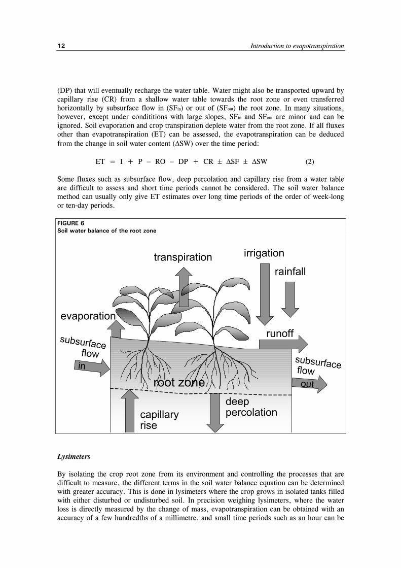
Evapotranspiration can also be determined by measuring the various components of the soil water balance. The method consists of assessing the incoming and outgoing water flux into the crop root zone over some time period (Figure 6). Irrigation (I) and rainfall (P) add water to the root zone. Part of I and P might be lost by surface runoff (RO) and by deep percolation
Introduction to evapotranspiration
12
(DP) that will eventually recharge the water table. Water might also be transported upward by capillary rise (CR) from a shallow water table towards the root zone or even transferred horizontally by subsurface flow in (SFin) or out of (SFout) the root zone. In many situations, however, except under condititions with large slopes, SFin and SFout are minor and can be ignored. Soil evaporation and crop transpiration deplete water from the root zone. If all fluxes other than evapotranspiration (ET) can be assessed, the evapotranspiration can be deduced from the change in soil water content (∆SW) over the time period: ET = I + P − RO − DP + CR ± ∆SF ± ∆SW (2) Some fluxes such as subsurface flow, deep percolation and capillary rise from a water table are difficult to assess and short time periods cannot be considered. The soil water balance method can usually only give ET estimates over long time periods of the order of week-long or ten-day periods. FIGURE 6 Soil water balance of the root zone
evaporation
transpiration irrigation
rainfall
root zonedeeppercolationcapillary
rise
in
out
flowflow
runoffsubsurfacesubsurface
Lysimeters By isolating the crop root zone from its environment and controlling the processes that are difficult to measure, the different terms in the soil water balance equation can be determined with greater accuracy. This is done in lysimeters where the crop grows in isolated tanks filled with either disturbed or undisturbed soil. In precision weighing lysimeters, where the water loss is directly measured by the change of mass, evapotranspiration can be obtained with an accuracy of a few hundredths of a millimetre, and small time periods such as an hour can be
Crop evapotranspiration
13
considered. In non-weighing lysimeters the evapotranspiration for a given time period is determined by deducting the drainage water, collected at the bottom of the lysimeters, from the total water input.
A requirement of lysimeters is that the vegetation both inside and immediately outside of the lysimeter be perfectly matched (same height and leaf area index). This requirement has historically not been closely adhered to in a majority of lysimeter studies and has resulted in severely erroneous and unrepresentative ETc and Kc data.
As lysimeters are difficult and expensive to construct and as their operation and maintenance require special care, their use is limited to specific research purposes. ET computed from meteorological data Owing to the difficulty of obtaining accurate field measurements, ET is commonly computed from weather data. A large number of empirical or semi-empirical equations have been developed for assessing crop or reference crop evapotranspiration from meteorological data. Some of the methods are only valid under specific climatic and agronomic conditions and cannot be applied under conditions different from those under which they were originally developed.
Numerous researchers have analysed the performance of the various calculation methods for different locations. As a result of an Expert Consultation held in May 1990, the FAO Penman-Monteith method is now recommended as the standard method for the definition and computation of the reference evapotranspiration, ETo. The ET from crop surfaces under standard conditions is determined by crop coefficients (Kc) that relate ETc to ETo. The ET from crop surfaces under non-standard conditions is adjusted by a water stress coefficient (Ks) and/or by modifying the crop coefficient. ET estimated from pan evaporation Evaporation from an open water surface provides an index of the integrated effect of radiation, air temperature, air humidity and wind on evapotranspiration. However, differences in the water and cropped surface produce significant differences in the water loss from an open water surface and the crop. The pan has proved its practical value and has been used successfully to estimate reference evapotranspiration by observing the evaporation loss from a water surface and applying empirical coefficients to relate pan evaporation to ETo. The procedure is outlined in Chapter 3.

Introduction to evapotranspiration
14
Crop evapotranspiration
15
Part A
Reference evapotranspiration (ETo)
Part A deals with the evapotranspiration from the reference surface, the so-called reference crop evapotranspiration or reference evapotranspiration, denoted as ETo. The reference surface is a hypothetical grass reference crop with an assumed crop height of 0.12 m, a fixed surface resistance of 70 s m
-1 and an albedo of 0.23. The reference surface closely resembles an extensive surface of green,
well-watered grass of uniform height, actively growing and completely shading the ground. The fixed surface resistance of 70 s m-1 implies a moderately dry soil surface resulting from about a weekly irrigation frequency. ETo can be computed from meteorological data. As a result of an Expert Consultation held in May 1990, the FAO Penman-Monteith method is now recommended as the sole standard method for the definition and computation of the reference evapotranspiration. The FAO Penman-Monteith method requires radiation, air temperature, air humidity and wind speed data. Calculation procedures to derive climatic parameters from meteorological data and to estimate missing meteorological variables required for calculating ETo are presented in this Part (Chapter 3). The calculation procedures in this Publication allow for estimation of ETo with the FAO Penman-Monteith method under all circumstances, even in the case of missing climatic data. ETo can also be estimated from pan evaporation. Pans have proved their practical value and have been used successfully to estimate ETo by observing the water loss from the pan and using empirical coefficients to relate pan evaporation to ETo. However, special precautions and management must be applied.

16
Crop evapotranspiration
17
Chapter 2
FAO Penman-Monteith equation
This chapter introduces the user to the need to standardize one method to compute reference evapotranspiration (ETo) from meteorological data. The FAO Penman-Monteith method is recommended as the sole ETo method for determining reference evapotranspiration. The method, its derivation, the required meteorological data and the corresponding definition of the reference surface are described in this chapter. NEED FOR A STANDARD ETO METHOD A large number of more or less empirical methods have been developed over the last 50 years by numerous scientists and specialists worldwide to estimate evapotranspiration from different climatic variables. Relationships were often subject to rigorous local calibrations and proved to have limited global validity. Testing the accuracy of the methods under a new set of conditions is laborious, time-consuming and costly, and yet evapotranspiration data are frequently needed at short notice for project planning or irrigation scheduling design. To meet this need, guidelines were developed and published in the FAO Irrigation and Drainage Paper No. 24 'Crop water requirements'. To accommodate users with different data availability, four methods were presented to calculate the reference crop evapotranspiration (ETo): the Blaney-Criddle, radiation, modified Penman and pan evaporation methods. The modified Penman method was considered to offer the best results with minimum possible error in relation to a living grass reference crop. It was expected that the pan method would give acceptable estimates, depending on the location of the pan. The radiation method was suggested for areas where available climatic data include measured air temperature and sunshine, cloudiness or radiation, but not measured wind speed and air humidity. Finally, the publication proposed the use of the Blaney-Criddle method for areas where available climatic data cover air temperature data only.
These climatic methods to calculate ETo were all calibrated for ten-day or monthly calculations, not for daily or hourly calculations. The Blaney-Criddle method was recommended for periods of one month or longer. For the pan method it was suggested that calculations should be done for periods of ten days or longer. Users have not always respected these conditions and calculations have often been done on daily time steps.
Advances in research and the more accurate assessment of crop water use have revealed
weaknesses in the methodologies. Numerous researchers analysed the performance of the four methods for different locations. Although the results of such analyses could have been influenced by site or measurement conditions or by bias in weather data collection, it became evident that the proposed methods do not behave the same way in different locations around the world. Deviations from computed to observed values were often found to exceed ranges indicated by FAO. The modified Penman was frequently found to overestimate ETo, even by
FAO Penman-Monteith equation
18
up to 20% for low evaporative conditions. The other FAO recommended equations showed variable adherence to the reference crop evapotranspiration standard of grass.
To evaluate the performance of these and other estimation procedures under different climatological conditions, a major study was undertaken under the auspices of the Committee on Irrigation Water Requirements of the American Society of Civil Engineers (ASCE). The ASCE study analysed the performance of 20 different methods, using detailed procedures to assess the validity of the methods compared to a set of carefully screened lysimeter data from 11 locations with variable climatic conditions. The study proved very revealing and showed the widely varying performance of the methods under different climatic conditions. In a parallel study commissioned by the European Community, a consortium of European research institutes evaluated the performance of various evapotranspiration methods using data from different lysimeter studies in Europe.
The studies confirm the overestimation of the modified Penman introduced in FAO Irrigation and Drainage Paper No. 24, and the variable performance of the different methods depending on their adaptation to local conditions. The comparative studies may be summarized as follows: • The Penman methods may require local calibration of the wind function to achieve
satisfactory results. • The radiation methods show good results in humid climates where the aerodynamic term
is relatively small, but performance in arid conditions is erratic and tends to underestimate evapotranspiration.
• Temperature methods remain empirical and require local calibration in order to achieve satisfactory results. A possible exception is the 1985 Hargreaves’ method which has shown reasonable ETo results with a global validity.
• Pan evapotranspiration methods clearly reflect the shortcomings of predicting crop evapotranspiration from open water evaporation. The methods are susceptible to the microclimatic conditions under which the pans are operating and the rigour of station maintenance. Their performance proves erratic.
• The relatively accurate and consistent performance of the Penman-Monteith approach in both arid and humid climates has been indicated in both the ASCE and European studies.
The analysis of the performance of the various calculation methods reveals the need for formulating a standard method for the computation of ETo. The FAO Penman-Monteith method is recommended as the sole standard method. It is a method with strong likelihood of correctly predicting ETo in a wide range of locations and climates and has provision for application in data-short situations. The use of older FAO or other reference ET methods is no longer encouraged. FORMULATION OF THE PENMAN-MONTEITH EQUATION Penman-Monteith equation In 1948, Penman combined the energy balance with the mass transfer method and derived an equation to compute the evaporation from an open water surface from standard climatological records of sunshine, temperature, humidity and wind speed. This so-called combination
Crop evapotranspiration
19
method was further developed by many researchers and extended to cropped surfaces by introducing resistance factors. The resistance nomenclature distinguishes between aerodynamic resistance and surface resistance factors (Figure 7). The surface resistance parameters are often combined into one parameter, the ‘bulk’ surface resistance parameter which operates in series with the aerodynamic resistance. The surface resistance, rs, describes the resistance of vapour flow through stomata openings, total leaf area and soil surface. The aerodynamic resistance, ra, describes the resistance from the vegetation upward and involves friction from air flowing over vegetative surfaces. Although the exchange process in a vegetation layer is too complex to be fully described by the two resistance factors, good correlations can be obtained between measured and calculated evapotranspiration rates, especially for a uniform grass reference surface.
The Penman-Monteith form of the combination equation is:
���
����
�+γ+∆
−ρ+−∆
=λ
a
s
a
aspan
rr
1
r)e(e
cG)(RET (3)
where Rn is the net radiation, G is the soil heat flux, (es - ea) represents the vapour pressure deficit of the air, ρa is the mean air density at constant pressure, cp is the specific heat of the air, ∆ represents the slope of the saturation vapour pressure temperature relationship, γ is the
FIGURE 7 Simplified representation of the (bulk) surface and aerodynamic resistances for water vapour flow
soil
stomatal
air flo
w
r
r
s
a
(bulk) surface resistance
aerodynamicresistance
referencelevel
evaporatingsurface
cuticular
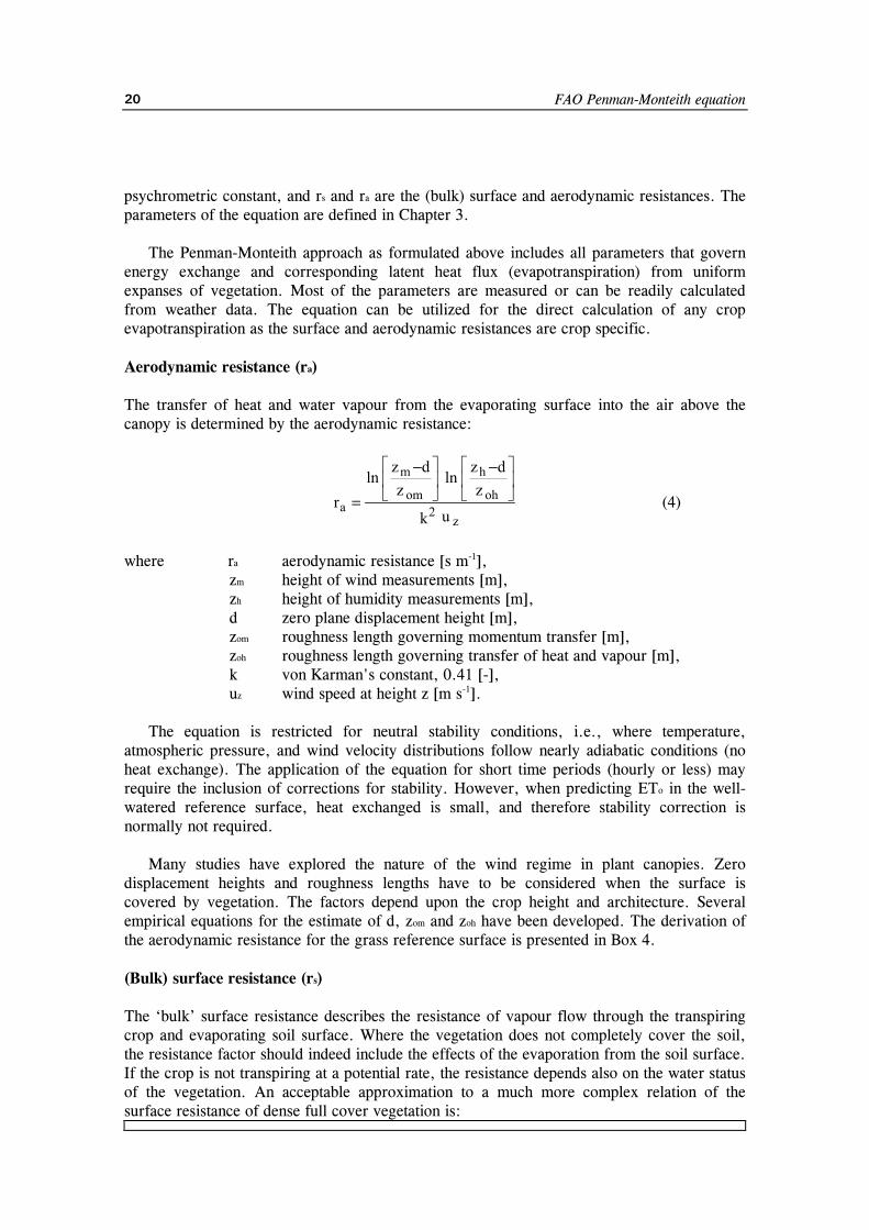
FAO Penman-Monteith equation
20
psychrometric constant, and rs and ra are the (bulk) surface and aerodynamic resistances. The parameters of the equation are defined in Chapter 3. The Penman-Monteith approach as formulated above includes all parameters that govern energy exchange and corresponding latent heat flux (evapotranspiration) from uniform expanses of vegetation. Most of the parameters are measured or can be readily calculated from weather data. The equation can be utilized for the direct calculation of any crop evapotranspiration as the surface and aerodynamic resistances are crop specific. Aerodynamic resistance (ra) The transfer of heat and water vapour from the evaporating surface into the air above the canopy is determined by the aerodynamic resistance:
z
2oh
h
om
m
a uk
zdz
lnz
dzln
r��
���
� −��
���
� −
= (4)
where ra aerodynamic resistance [s m-1],
zm height of wind measurements [m], zh height of humidity measurements [m], d zero plane displacement height [m], zom roughness length governing momentum transfer [m], zoh roughness length governing transfer of heat and vapour [m], k von Karman's constant, 0.41 [-], uz wind speed at height z [m s-1].
The equation is restricted for neutral stability conditions, i.e., where temperature, atmospheric pressure, and wind velocity distributions follow nearly adiabatic conditions (no heat exchange). The application of the equation for short time periods (hourly or less) may require the inclusion of corrections for stability. However, when predicting ETo in the well-watered reference surface, heat exchanged is small, and therefore stability correction is normally not required. Many studies have explored the nature of the wind regime in plant canopies. Zero displacement heights and roughness lengths have to be considered when the surface is covered by vegetation. The factors depend upon the crop height and architecture. Several empirical equations for the estimate of d, zom and zoh have been developed. The derivation of the aerodynamic resistance for the grass reference surface is presented in Box 4. (Bulk) surface resistance (rs) The ‘bulk’ surface resistance describes the resistance of vapour flow through the transpiring crop and evaporating soil surface. Where the vegetation does not completely cover the soil, the resistance factor should indeed include the effects of the evaporation from the soil surface. If the crop is not transpiring at a potential rate, the resistance depends also on the water status of the vegetation. An acceptable approximation to a much more complex relation of the surface resistance of dense full cover vegetation is:
Crop evapotranspiration
21
BOX 4 The aerodynamic resistance for a grass reference surface For a wide range of crops the zero plane displacement height, d [m], and the roughness length governing momentum transfer, zom [m], can be estimated from the crop height h [m] by the following equations:
d = 2/3 h
zom = 0.123 h The roughness length governing transfer of heat and vapour, zoh [m], can be approximated by:
zoh = 0.1 zom Assuming a constant crop height of 0.12 m and a standardized height for wind speed, temperature and humidity at 2 m (zm = zh = 2 m), the aerodynamic resistance ra [s m-1] for the grass reference surface becomes (Eq. 4):
222a u
208u(0.41)
(0.12)0.123(0.1)(0.12)2/3-2ln
(0.12)0.123(0.12)2/3-2ln
r =��
���
���
���
�
=
where u2 is the wind speed [m s-1] at 2 m.
active
1s LAI
rr = (5)
where rs (bulk) surface resistance [s m-1],
rl bulk stomatal resistance of the well-illuminated leaf [s m-1], LAIactive active (sunlit) leaf area index [m2 (leaf area) m-2 (soil
surface)]. The Leaf Area Index (LAI), a dimensionless quantity, is the leaf area (upper side only) per unit area of soil below it. It is expressed as m2 leaf area per m2 ground area. The active LAI is the index of the leaf area that actively contributes to the surface heat and vapour transfer. It is generally the upper, sunlit portion of a dense canopy. The LAI values for various crops differ widely but values of 3-5 are common for many mature crops. For a given crop, green LAI changes throughout the season and normally reaches its maximum before or at flowering (Figure 8). LAI further depends on the plant density and the crop variety. The bulk stomatal resistance, rl, is the average resistance of an individual leaf. This resistance is crop specific and differs among crop varieties and crop management. It usually increases as the crop ages and begins to ripen. There is, however, a lack of consolidated information on changes in rl over time for the different crops. The information available in the literature on stomatal conductance or resistance is often oriented toward physiological or ecophysiological studies. The stomatal resistance, rl, is influenced by climate and by water availability. However, influences vary from one crop to another and different varieties can be affected differently. The resistance increases when the crop is water stressed and the soil water availability limits
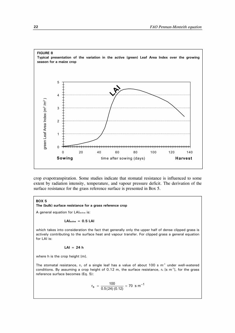
FAO Penman-Monteith equation
22
crop evapotranspiration. Some studies indicate that stomatal resistance is influenced to some extent by radiation intensity, temperature, and vapour pressure deficit. The derivation of the surface resistance for the grass reference surface is presented in Box 5.
BOX 5 The (bulk) surface resistance for a grass reference crop A general equation for LAIactive is:
LAIactive = 0.5 LAI which takes into consideration the fact that generally only the upper half of dense clipped grass is actively contributing to the surface heat and vapour transfer. For clipped grass a general equation for LAI is:
LAI = 24 h where h is the crop height [m]. The stomatal resistance, rl, of a single leaf has a value of about 100 s m-1 under well-watered conditions. By assuming a crop height of 0.12 m, the surface resistance, rs [s m-1], for the grass reference surface becomes (Eq. 5):
1s ms70
(0.12)24)(0.5100r −≈=
FIGURE 8 Typical presentation of the variation in the active (green) Leaf Area Index over the growingseason for a maize crop
Harvest
LAI
Sowing
0
1
2
3
4
5
0 20 40 60 80 100 120 140
time after sowing (days)
gree
n Le
af A
rea
Inde
x (m
2 /m
2 )
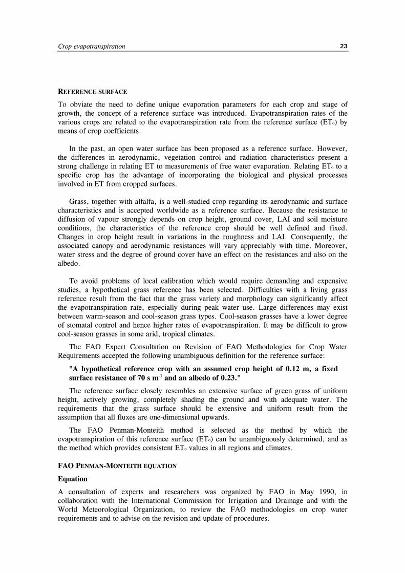
Crop evapotranspiration
23
REFERENCE SURFACE
To obviate the need to define unique evaporation parameters for each crop and stage of growth, the concept of a reference surface was introduced. Evapotranspiration rates of the various crops are related to the evapotranspiration rate from the reference surface (ETo) by means of crop coefficients. In the past, an open water surface has been proposed as a reference surface. However, the differences in aerodynamic, vegetation control and radiation characteristics present a strong challenge in relating ET to measurements of free water evaporation. Relating ETo to a specific crop has the advantage of incorporating the biological and physical processes involved in ET from cropped surfaces. Grass, together with alfalfa, is a well-studied crop regarding its aerodynamic and surface characteristics and is accepted worldwide as a reference surface. Because the resistance to diffusion of vapour strongly depends on crop height, ground cover, LAI and soil moisture conditions, the characteristics of the reference crop should be well defined and fixed. Changes in crop height result in variations in the roughness and LAI. Consequently, the associated canopy and aerodynamic resistances will vary appreciably with time. Moreover, water stress and the degree of ground cover have an effect on the resistances and also on the albedo. To avoid problems of local calibration which would require demanding and expensive studies, a hypothetical grass reference has been selected. Difficulties with a living grass reference result from the fact that the grass variety and morphology can significantly affect the evapotranspiration rate, especially during peak water use. Large differences may exist between warm-season and cool-season grass types. Cool-season grasses have a lower degree of stomatal control and hence higher rates of evapotranspiration. It may be difficult to grow cool-season grasses in some arid, tropical climates.
The FAO Expert Consultation on Revision of FAO Methodologies for Crop Water Requirements accepted the following unambiguous definition for the reference surface:
"A hypothetical reference crop with an assumed crop height of 0.12 m, a fixed surface resistance of 70 s m-1 and an albedo of 0.23."
The reference surface closely resembles an extensive surface of green grass of uniform height, actively growing, completely shading the ground and with adequate water. The requirements that the grass surface should be extensive and uniform result from the assumption that all fluxes are one-dimensional upwards.
The FAO Penman-Monteith method is selected as the method by which the evapotranspiration of this reference surface (ETo) can be unambiguously determined, and as the method which provides consistent ETo values in all regions and climates. FAO PENMAN-MONTEITH EQUATION
Equation
A consultation of experts and researchers was organized by FAO in May 1990, in collaboration with the International Commission for Irrigation and Drainage and with the World Meteorological Organization, to review the FAO methodologies on crop water requirements and to advise on the revision and update of procedures.
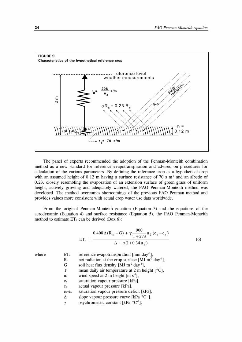
FAO Penman-Monteith equation
24
The panel of experts recommended the adoption of the Penman-Monteith combination method as a new standard for reference evapotranspiration and advised on procedures for calculation of the various parameters. By defining the reference crop as a hypothetical crop with an assumed height of 0.12 m having a surface resistance of 70 s m-1 and an albedo of 0.23, closely resembling the evaporation of an extension surface of green grass of uniform height, actively growing and adequately watered, the FAO Penman-Monteith method was developed. The method overcomes shortcomings of the previous FAO Penman method and provides values more consistent with actual crop water use data worldwide.
From the original Penman-Monteith equation (Equation 3) and the equations of the aerodynamic (Equation 4) and surface resistance (Equation 5), the FAO Penman-Monteith method to estimate ETo can be derived (Box 6):
)u34.01(
)ee(u273T
900)GR(408.0ET
2
as2n
o +γ+∆
−+
γ+−∆= (6)
where ETo reference evapotranspiration [mm day-1],
Rn net radiation at the crop surface [MJ m-2 day-1], G soil heat flux density [MJ m-2 day-1], T mean daily air temperature at 2 m height [°C], u2 wind speed at 2 m height [m s-1], es saturation vapour pressure [kPa], ea actual vapour pressure [kPa], es-ea saturation vapour pressure deficit [kPa], ∆ slope vapour pressure curve [kPa °C-1], γ psychrometric constant [kPa °C-1].
FIGURE 9 Characteristics of the hypothetical reference crop
weather measurements
2 m
0.12 m
r =a208
u s/m
r = 70 s/ms
radiation
solar
αRss
2
d + zoh
= 0.23 Rs R
h =
reference level
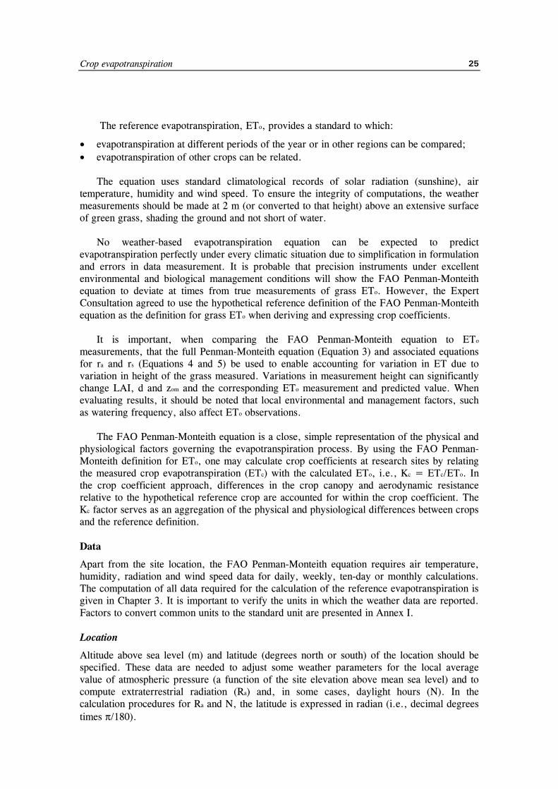
Crop evapotranspiration
25
The reference evapotranspiration, ETo, provides a standard to which:
• evapotranspiration at different periods of the year or in other regions can be compared; • evapotranspiration of other crops can be related.
The equation uses standard climatological records of solar radiation (sunshine), air temperature, humidity and wind speed. To ensure the integrity of computations, the weather measurements should be made at 2 m (or converted to that height) above an extensive surface of green grass, shading the ground and not short of water.
No weather-based evapotranspiration equation can be expected to predict evapotranspiration perfectly under every climatic situation due to simplification in formulation and errors in data measurement. It is probable that precision instruments under excellent environmental and biological management conditions will show the FAO Penman-Monteith equation to deviate at times from true measurements of grass ETo. However, the Expert Consultation agreed to use the hypothetical reference definition of the FAO Penman-Monteith equation as the definition for grass ETo when deriving and expressing crop coefficients.
It is important, when comparing the FAO Penman-Monteith equation to ETo measurements, that the full Penman-Monteith equation (Equation 3) and associated equations for ra and rs (Equations 4 and 5) be used to enable accounting for variation in ET due to variation in height of the grass measured. Variations in measurement height can significantly change LAI, d and zom and the corresponding ETo measurement and predicted value. When evaluating results, it should be noted that local environmental and management factors, such as watering frequency, also affect ETo observations.
The FAO Penman-Monteith equation is a close, simple representation of the physical and physiological factors governing the evapotranspiration process. By using the FAO Penman-Monteith definition for ETo, one may calculate crop coefficients at research sites by relating the measured crop evapotranspiration (ETc) with the calculated ETo, i.e., Kc = ETc/ETo. In the crop coefficient approach, differences in the crop canopy and aerodynamic resistance relative to the hypothetical reference crop are accounted for within the crop coefficient. The Kc factor serves as an aggregation of the physical and physiological differences between crops and the reference definition. Data
Apart from the site location, the FAO Penman-Monteith equation requires air temperature, humidity, radiation and wind speed data for daily, weekly, ten-day or monthly calculations. The computation of all data required for the calculation of the reference evapotranspiration is given in Chapter 3. It is important to verify the units in which the weather data are reported. Factors to convert common units to the standard unit are presented in Annex I. Location
Altitude above sea level (m) and latitude (degrees north or south) of the location should be specified. These data are needed to adjust some weather parameters for the local average value of atmospheric pressure (a function of the site elevation above mean sea level) and to compute extraterrestrial radiation (Ra) and, in some cases, daylight hours (N). In the calculation procedures for Ra and N, the latitude is expressed in radian (i.e., decimal degrees times π/180).
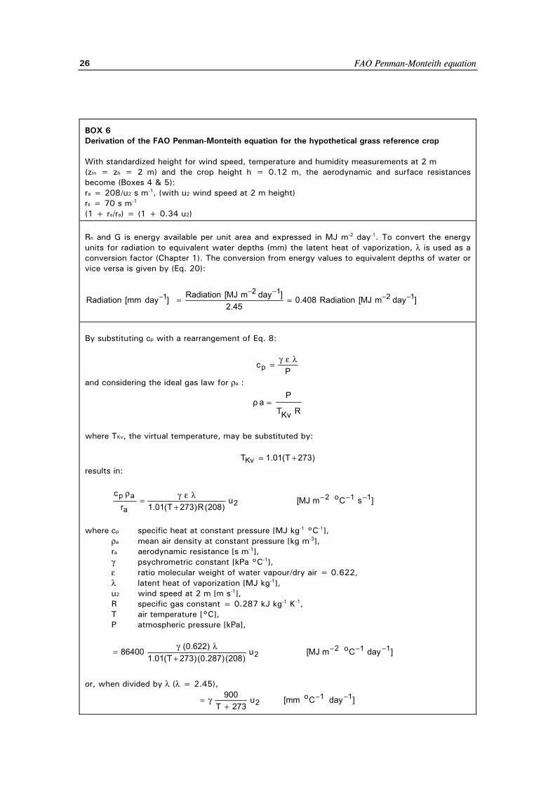
FAO Penman-Monteith equation
26
BOX 6 Derivation of the FAO Penman-Monteith equation for the hypothetical grass reference crop With standardized height for wind speed, temperature and humidity measurements at 2 m (zm = zh = 2 m) and the crop height h = 0.12 m, the aerodynamic and surface resistances become (Boxes 4 & 5): ra = 208/u2 s m-1, (with u2 wind speed at 2 m height) rs = 70 s m-1 (1 + rs/ra) = (1 + 0.34 u2) Rn and G is energy available per unit area and expressed in MJ m-2 day-1. To convert the energy units for radiation to equivalent water depths (mm) the latent heat of vaporization, λ is used as a conversion factor (Chapter 1). The conversion from energy values to equivalent depths of water or vice versa is given by (Eq. 20):
]daymMJ[Radiation408.045.2
]daymMJ[Radiation]daymm[Radiation 1212
1 −−−−
− =≈
By substituting cp with a rearrangement of Eq. 8:
Pcp
λεγ=
and considering the ideal gas law for ρa :
RKvT
Paρ =
where TKv, the virtual temperature, may be substituted by:
)273T(01.1TKv +=
results in:
]sCmMJ[u)208(R)273T(01.1r
c 11o22
a
ap −−−+
λεγ=
ρ
where cp specific heat at constant pressure [MJ kg-1 °C-1], ρa mean air density at constant pressure [kg m-3], ra aerodynamic resistance [s m-1], γ psychrometric constant [kPa °C-1], ε ratio molecular weight of water vapour/dry air = 0.622, λ latent heat of vaporization [MJ kg-1], u2 wind speed at 2 m [m s-1], R specific gas constant = 0.287 kJ kg-1 K-1, T air temperature [°C], P atmospheric pressure [kPa],
]dayCmMJ[u)208()287.0()273T(01.1
)622.0(86400 11o22
−−−+
λγ=
or, when divided by λ (λ = 2.45),
]dayCmm[u273T
900 11o2
−−+
γ≈
Crop evapotranspiration
27
A positive value is used for the northern hemisphere and a negative value for the southern hemisphere. Temperature The (average) daily maximum and minimum air temperatures in degrees Celsius (°C) are required. Where only (average) mean daily temperatures are available, the calculations can still be executed but some underestimation of ETo will probably occur due to the non-linearity of the saturation vapour pressure - temperature relationship (Figure 11). Using mean air temperature instead of maximum and minimum air temperatures yields a lower saturation vapour pressure es, and hence a lower vapour pressure difference (es - ea), and a lower reference evapotranspiration estimate. Humidity The (average) daily actual vapour pressure, ea, in kilopascals (kPa) is required. The actual vapour pressure, where not available, can be derived from maximum and minimum relative humidity (%), psychrometric data (dry and wet bulb temperatures in °C) or dewpoint temperature (°C) according to the procedures outlined in Chapter 3. Radiation The (average) daily net radiation expressed in megajoules per square metre per day (MJ m-2 day-1) is required. These data are not commonly available but can be derived from the (average) shortwave radiation measured with a pyranometer or from the (average) daily actual duration of bright sunshine (hours per day) measured with a (Campbell-Stokes) sunshine recorder. The calculation procedures are outlined in Chapter 3. Wind speed The (average) daily wind speed in metres per second (m s-1) measured at 2 m above the ground level is required. It is important to verify the height at which wind speed is measured, as wind speeds measured at different heights above the soil surface differ. The calculation procedure to adjust wind speed to the standard height of 2 m is presented in Chapter 3. Missing climatic data Situations might occur where data for some weather variables are missing. The use of an alternative ETo calculation procedure, requiring only limited meteorological parameters, should generally be avoided. It is recommended that one calculate ETo using the standard FAO Penman-Monteith method after resolving the specific problem of the missing data. Procedures for estimating missing climatic data are outlined in Chapter 3. Differences between ETo values obtained with the FAO Penman-Monteith equation with, on the one hand, a limited data set and, on the other hand, a full data set, are expected to be smaller than or of similar magnitude to the differences resulting from the use of an alternative ETo equation.
Even where the data set contains only maximum and minimum air temperature it is still possible to obtain reasonable estimates of ten-day or monthly ETo with the FAO Penman-Monteith equation. As outlined in Chapter 3, radiation data can be derived from the air temperature difference, or, along with wind speed and humidity data, can be imported from a

FAO Penman-Monteith equation
28
nearby weather station. Humidity data can also be estimated from daily minimum air temperature. After evaluating the validity of the use of data from another station, ten-day or monthly estimates of ETo can be calculated.
The procedures for estimating missing data should be validated at the regional level. This can be done for weather stations with full data sets by comparing ETo calculated with full and with limited data sets. The ratio should be close to one. Where the ratio deviates significantly from one, the ratio can be used as a correction factor for estimates made with the limited data set. Where the standard error of estimate exceeds 20% of the mean ETo, a sensitivity analysis should be performed to determine causes (and limits) for the method utilized to import the missing data. A validation should be completed for each month and variable, for the monthly as well as for the daily estimates.
Crop evapotranspiration
29
Chapter 3
Meteorological data The methods for calculating evapotranspiration from meteorological data require various climatological and physical parameters. Some of the data are measured directly in weather stations. Other parameters are related to commonly measured data and can be derived with the help of a direct or empirical relationship. This chapter discusses the source, measurement and computation of all data required for the calculation of the reference evapotranspiration by means of the FAO Penman-Monteith method. Different examples illustrate the various calculation procedures. Appropriate procedures for estimating missing data are also provided.
Meteorological data can be expressed in several units. Conversion factors between various units and standard S.I. units are given in Annex 1. Climatic parameters, calculated by means of the equations presented in this chapter are tabulated and displayed for different meteorological conditions in Annex 2. Only the standardized relationships are presented in this chapter. The background of certain relationships and more information about certain procedures are given in Annex 3. Annexes 4, 5 and 6 list procedures for the statistical analysis, assessment, correction and completion of partial or missing weather data. METEOROLOGICAL FACTORS DETERMINING ET
The meteorological factors determining evapotranspiration are weather parameters which provide energy for vaporization and remove water vapour from the evaporating surface. The principal weather parameters to consider are presented below. Solar radiation
The evapotranspiration process is determined by the amount of energy available to vaporize water. Solar radiation is the largest energy source and is able to change large quantities of liquid water into water vapour. The potential amount of radiation that can reach the evaporating surface is determined by its location and time of the year. Due to differences in the position of the sun, the potential radiation differs at various latitudes and in different seasons. The actual solar radiation reaching the evaporating surface depends on the turbidity of the atmosphere and the presence of clouds which reflect and absorb major parts of the radiation. When assessing the effect of solar radiation on evapotranspiration, one should also bear in mind that not all available energy is used to vaporize water. Part of the solar energy is used to heat up the atmosphere and the soil profile. Air temperature
The solar radiation absorbed by the atmosphere and the heat emitted by the earth increase the air temperature. The sensible heat of the surrounding air transfers energy to the crop and exerts as such a controlling influence on the rate of evapotranspiration. In sunny, warm weather the loss of water by evapotranspiration is greater than in cloudy and cool weather.
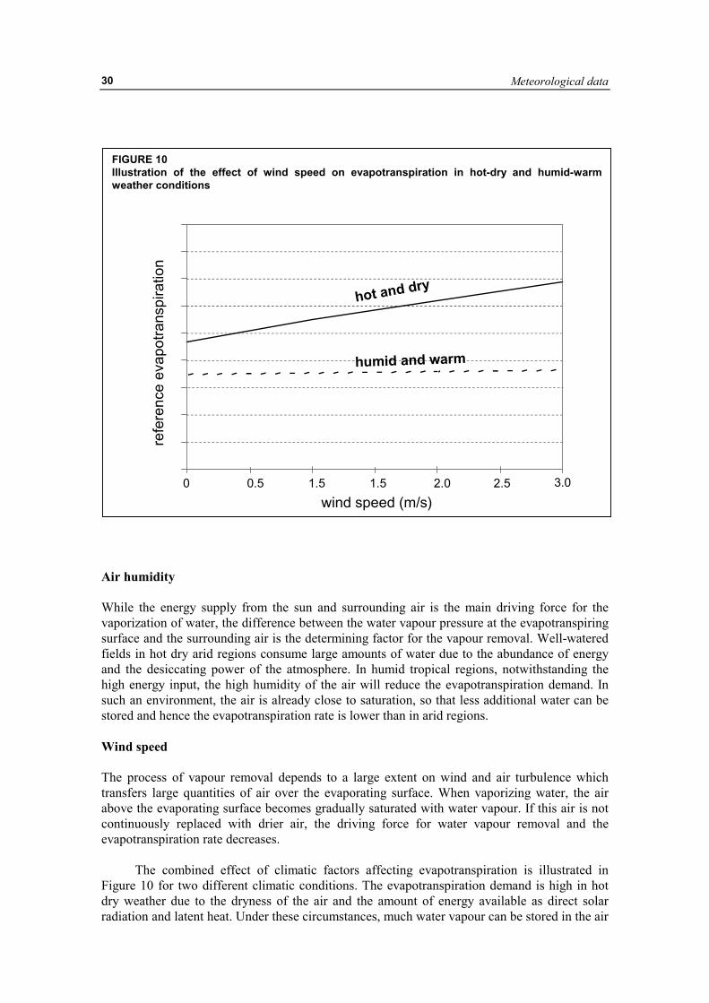
Meteorological data
30
Air humidity While the energy supply from the sun and surrounding air is the main driving force for the vaporization of water, the difference between the water vapour pressure at the evapotranspiring surface and the surrounding air is the determining factor for the vapour removal. Well-watered fields in hot dry arid regions consume large amounts of water due to the abundance of energy and the desiccating power of the atmosphere. In humid tropical regions, notwithstanding the high energy input, the high humidity of the air will reduce the evapotranspiration demand. In such an environment, the air is already close to saturation, so that less additional water can be stored and hence the evapotranspiration rate is lower than in arid regions. Wind speed The process of vapour removal depends to a large extent on wind and air turbulence which transfers large quantities of air over the evaporating surface. When vaporizing water, the air above the evaporating surface becomes gradually saturated with water vapour. If this air is not continuously replaced with drier air, the driving force for water vapour removal and the evapotranspiration rate decreases.
The combined effect of climatic factors affecting evapotranspiration is illustrated in Figure 10 for two different climatic conditions. The evapotranspiration demand is high in hot dry weather due to the dryness of the air and the amount of energy available as direct solar radiation and latent heat. Under these circumstances, much water vapour can be stored in the air
FIGURE 10 Illustration of the effect of wind speed on evapotranspiration in hot-dry and humid-warm weather conditions
0 1.5 2.0 3.0
wind speed (m/s)
refe
renc
e ev
apot
rans
pira
tion
humid and warm
hot and dry
1.5 2.50.5
Crop evapotranspiration
31
while wind may promote the transport of water allowing more water vapour to be taken up. On the other hand, under humid weather conditions, the high humidity of the air and the presence of clouds cause the evapotranspiration rate to be lower. The effect on evapotranspiration of increasing wind speeds for the two different climatic conditions is illustrated by the slope of the curves in Figure 10. The drier the atmosphere, the larger the effect on ET and the greater the slope of the curve. For humid conditions, the wind can only replace saturated air with slightly less saturated air and remove heat energy. Consequently, the wind speed affects the evapotranspiration rate to a far lesser extent than under arid conditions where small variations in wind speed may result in larger variations in the evapotranspiration rate. ATMOSPHERIC PARAMETERS
Several relationships are available to express climatic parameters. The effect of the principal weather parameters on evapotranspiration can be assessed with the help of these equations. Some of the relationships require parameters which express a specific characteristic of the atmosphere. Before studying the four principal weather parameters, some atmospheric parameters will be discussed. Atmospheric pressure (P) The atmospheric pressure, P, is the pressure exerted by the weight of the earth's atmosphere. Evaporation at high altitudes is promoted due to low atmospheric pressure as expressed in the psychrometric constant. The effect is, however, small and in the calculation procedures, the average value for a location is sufficient. A simplification of the ideal gas law, assuming 20°C for a standard atmosphere, can be employed to calculate P:
26.5
293z0065.02933.101P ��
���
� −= (7)
where P atmospheric pressure [kPa],
z elevation above sea level [m], Values for atmospheric pressure as a function of altitude are given in Annex 2 (Table 2.1). Latent heat of vaporization (λλλλ) The latent heat of vaporization, λ, expresses the energy required to change a unit mass of water from liquid to water vapour in a constant pressure and constant temperature process. The value of the latent heat varies as a function of temperature. At a high temperature, less energy will be required than at lower temperatures. As λ varies only slightly over normal temperature ranges a single value of 2.45 MJ kg-1 is taken in the simplification of the FAO Penman-Monteith equation. This is the latent heat for an air temperature of about 20°C. Psychrometric constant (γγγγ) The psychrometric constant, γ, is given by:
Meteorological data
32
P10x665.0Pc 3p −=
λε=γ (8)
where γ psychrometric constant [kPa °C-1],
P atmospheric pressure [kPa], λ latent heat of vaporization, 2.45 [MJ kg-1], cp specific heat at constant pressure, 1.013 10-3 [MJ kg-1 °C-1], ε ratio molecular weight of water vapour/dry air = 0.622.
The specific heat at constant pressure is the amount of energy required to increase the
temperature of a unit mass of air by one degree at constant pressure. Its value depends on the composition of the air, i.e., on its humidity. For average atmospheric conditions a value cp = 1.013 10-3 MJ kg-1 °C-1 can be used. As an average atmospheric pressure is used for each location (Equation 7), the psychrometric constant is kept constant for each location. Values for the psychrometric constant as a function of altitude are given in Annex 2 (Table 2.2).
EXAMPLE 2 Determination of atmospheric parameters. Determine the atmospheric pressure and the psychrometric constant at an elevation of 1 800 m. With: From Eq. 7: From Eq. 8:
z = P = 101.3 [(293 - (0.0065) 1800)/293]5.26 = γ = 0.665 10-3 (81.8) =
1 800 81.8
0.054
m kPa kPa °C-1
The average value of the atmospheric pressure is 81.8 kPa. The psychrometric constant, γ, is 0.054 kPa/°C.
AIR TEMPERATURE Agrometeorology is concerned with the air temperature near the level of the crop canopy. In traditional and modern automatic weather stations the air temperature is measured inside shelters (Stevenson screens or ventilated radiation shields) placed in line with World Meteorological Organization (WMO) standards at 2 m above the ground. The shelters are designed to protect the instruments from direct exposure to solar heating. The louvered construction allows free air movement around the instruments. Air temperature is measured with thermometers, thermistors or thermocouples mounted in the shelter. Minimum and maximum thermometers record the minimum and maximum air temperature over a 24-hour period. Thermographs plot the instantaneous temperature over a day or week. Electronic weather stations often sample air temperature each minute and report hourly averages in addition to 24-hour maximum and minimum values.
Due to the non-linearity of humidity data required in the FAO Penman-Monteith equation, the vapour pressure for a certain period should be computed as the mean between the vapour pressure at the daily maximum and minimum air temperatures of that period. The daily maximum air temperature (Tmax) and daily minimum air temperature (Tmin) are, respectively, the maximum and minimum air temperature observed during the 24-hour period, beginning at midnight. Tmax and Tmin for longer periods such as weeks, 10-day's or months are obtained by dividing the sum of the respective daily values by the number of days in the period. The mean
Crop evapotranspiration
33
daily air temperature (Tmean) is only employed in the FAO Penman-Monteith equation to calculate the slope of the saturation vapour pressure curves (∆) and the impact of mean air density (Pa) as the effect of temperature variations on the value of the climatic parameter is small in these cases. For standardization, Tmean for 24-hour periods is defined as the mean of the daily maximum (Tmax) and minimum temperatures (Tmin) rather than as the average of hourly temperature measurements.
2
TTT minmax
mean+
= (9)
The temperature is given in degrees Celsius (°C) or Fahrenheit (°F). The conversion table
is given in Annex 1. In some calculation procedures, temperature is required in Kelvin (K), which can be obtained by adding 273.16 to the temperature expressed in degrees Celsius (in practice K = °C + 273.16). The Kelvin and Celsius scale have the same scale interval. AIR HUMIDITY Concepts The water content of the air can be expressed in several ways. In agrometeorology, vapour pressure, dewpoint temperature and relative humidity are common expressions to indicate air humidity. Vapour pressure Water vapour is a gas and its pressure contributes to the total atmospheric pressure. The amount of water in the air is related directly to the partial pressure exerted by the water vapour in the air and is therefore a direct measure of the air water content.
In standard S.I. units, pressure is no longer expressed in centimetre of water, millimetre of mercury, bars, atmosphere, etc., but in pascals (Pa). Conversion factors between various units and Pa are given in Annex 1. As a pascal refers to a relatively small force (1 newton) applied on a relatively large surface (1 m2), multiples of the basic unit are often used. In this handbook, vapour pressure is expressed in kilopascals (kPa = 1 000 Pa).
When air is enclosed above an evaporating water surface, an equilibrium is reached between the water molecules escaping and returning to the water reservoir. At that moment, the air is said to be saturated since it cannot store any extra water molecules. The corresponding pressure is called the saturation vapour pressure (eo(T) ). The number of water molecules that can be stored in the air depends on the temperature (T). The higher the air temperature, the higher the storage capacity, the higher its saturation vapour pressure (Figure 11). As can be seen from Figure 11, the slope of the curve changes exponentially with temperature. At low temperatures, the slope is small and varies only slightly as the temperature rises. At high temperatures, the slope is large and small changes in T result in large changes in slope. The slope of the saturation vapour pressure curve, ∆, is an important parameter in describing vaporization and is required in the equations for calculating ETo from climatic data.
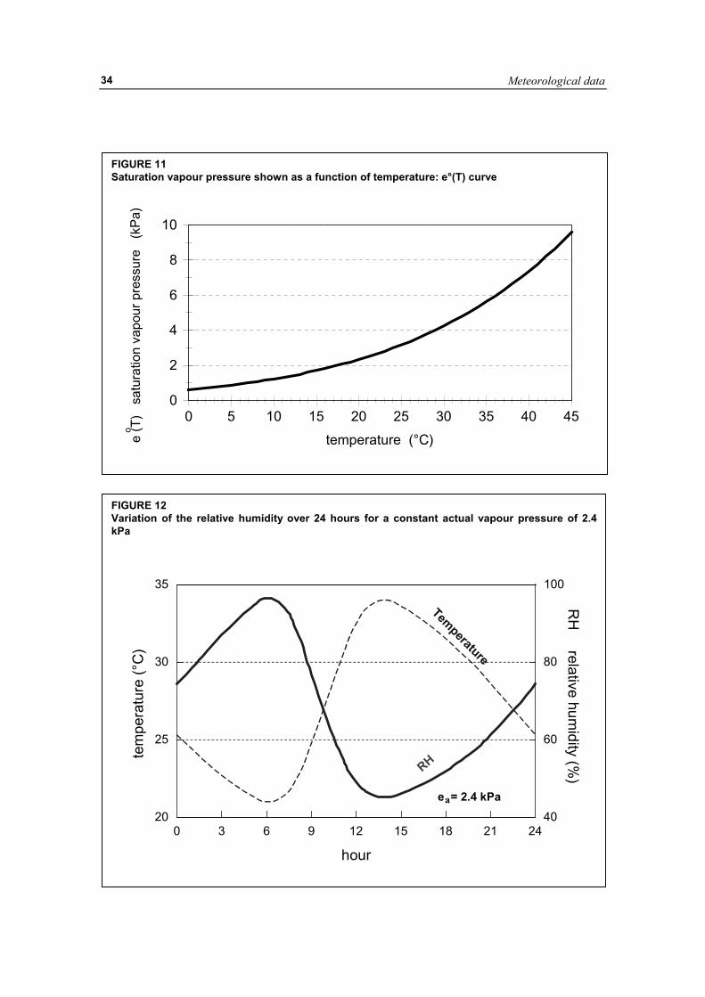
Meteorological data
34
FIGURE 11 Saturation vapour pressure shown as a function of temperature: e°(T) curve
0 5 10 15 20 25 30 35 40 45temperature (°C)
0
2
4
6
8
10
e (T
) s
atur
atio
n va
pour
pre
ssur
e (
kPa)
o
FIGURE 12 Variation of the relative humidity over 24 hours for a constant actual vapour pressure of 2.4kPa
0 3 6 9 12 15 18 21 24
hour
20
25
30
35
tem
pera
ture
(°C
)
40
60
80
100
RH
relative humidity (%
)RH
Temperature
e = 2.4 kPaa
Crop evapotranspiration
35
The actual vapour pressure (ea ) is the vapour pressure exerted by the water in the air. When the air is not saturated, the actual vapour pressure will be lower than the saturation vapour pressure. The difference between the saturation and actual vapour pressure is called the vapour pressure deficit or saturation deficit and is an accurate indicator of the actual evaporative capacity of the air. Dewpoint temperature The dewpoint temperature is the temperature to which the air needs to be cooled to make the air saturated. The actual vapour pressure of the air is the saturation vapour pressure at the dewpoint temperature. The drier the air, the larger the difference between the air temperature and dewpoint temperature. Relative humidity The relative humidity (RH) expresses the degree of saturation of the air as a ratio of the actual (ea) to the saturation (eo(T)) vapour pressure at the same temperature (T):
(T)oeae
100RH = (10)
Relative humidity is the ratio between the amount of water the ambient air actually holds
and the amount it could hold at the same temperature. It is dimensionless and is commonly given as a percentage. Although the actual vapour pressure might be relatively constant throughout the day, the relative humidity fluctuates between a maximum near sunrise and a minimum around early afternoon (Figure 12). The variation of the relative humidity is the result of the fact that the saturation vapour pressure is determined by the air temperature. As the temperature changes during the day, the relative humidity also changes substantially. Measurement It is not possible to directly measure the actual vapour pressure. The vapour pressure is commonly derived from relative humidity or dewpoint temperature.
Relative humidity is measured directly with hygrometers. The measurement is based on the nature of some material such as hair, which changes its length in response to changes in air humidity, or using a capacitance plate, where the electric capacitance changes with RH. Vapour pressure can be measured indirectly with psychrometers which measure the temperature difference between two thermometers, the so-called dry and wet bulb thermometers. The dry bulb thermometer measures the temperature of the air. The bulb of the wet bulb thermometer is covered with a constantly saturated wick. Evaporation of water from the wick, requiring energy, lowers the temperature of the thermometer. The drier the air, the larger the evaporative cooling and the larger the temperature drop. The difference between the dry and wet bulb temperatures is called the wet bulb depression and is a measure of the air humidity.
The dewpoint temperature is measured with dewpoint meters. The underlying principle of some types of apparatus is the cooling of the ambient air until dew formation occurs. The corresponding temperature is the dewpoint temperature.
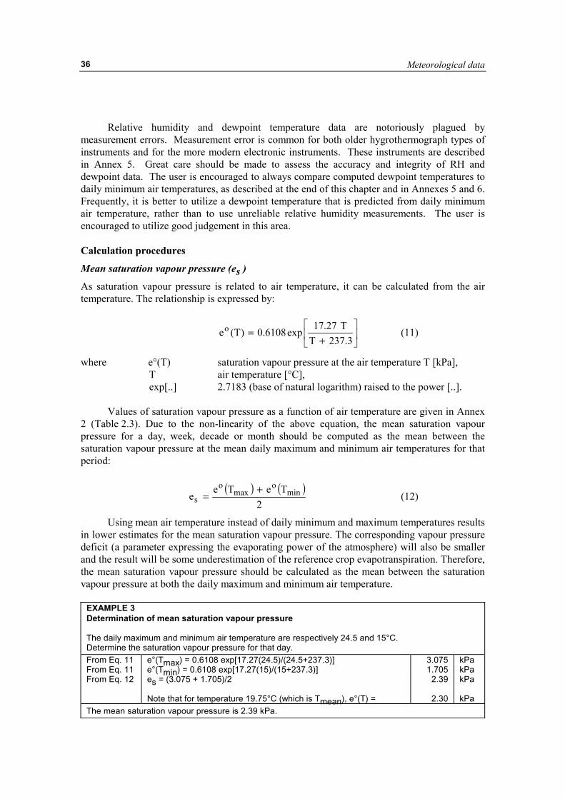
Meteorological data
36
Relative humidity and dewpoint temperature data are notoriously plagued by measurement errors. Measurement error is common for both older hygrothermograph types of instruments and for the more modern electronic instruments. These instruments are described in Annex 5. Great care should be made to assess the accuracy and integrity of RH and dewpoint data. The user is encouraged to always compare computed dewpoint temperatures to daily minimum air temperatures, as described at the end of this chapter and in Annexes 5 and 6. Frequently, it is better to utilize a dewpoint temperature that is predicted from daily minimum air temperature, rather than to use unreliable relative humidity measurements. The user is encouraged to utilize good judgement in this area. Calculation procedures
Mean saturation vapour pressure (es )
As saturation vapour pressure is related to air temperature, it can be calculated from the air temperature. The relationship is expressed by:
��
���
�
+=
3.237TT27.17exp6108.0)T(eo (11)
where e°(T) saturation vapour pressure at the air temperature T [kPa], T air temperature [°C], exp[..] 2.7183 (base of natural logarithm) raised to the power [..].
Values of saturation vapour pressure as a function of air temperature are given in Annex
2 (Table 2.3). Due to the non-linearity of the above equation, the mean saturation vapour pressure for a day, week, decade or month should be computed as the mean between the saturation vapour pressure at the mean daily maximum and minimum air temperatures for that period:
( ) ( )
2TeTe
e mino
maxo
s+
= (12)
Using mean air temperature instead of daily minimum and maximum temperatures results in lower estimates for the mean saturation vapour pressure. The corresponding vapour pressure deficit (a parameter expressing the evaporating power of the atmosphere) will also be smaller and the result will be some underestimation of the reference crop evapotranspiration. Therefore, the mean saturation vapour pressure should be calculated as the mean between the saturation vapour pressure at both the daily maximum and minimum air temperature.
EXAMPLE 3 Determination of mean saturation vapour pressure The daily maximum and minimum air temperature are respectively 24.5 and 15°C. Determine the saturation vapour pressure for that day. From Eq. 11 e°(Tmax) = 0.6108 exp[17.27(24.5)/(24.5+237.3)] 3.075 kPa From Eq. 11 e°(Tmin) = 0.6108 exp[17.27(15)/(15+237.3)] 1.705 kPa From Eq. 12 es = (3.075 + 1.705)/2
Note that for temperature 19.75°C (which is Tmean), e°(T) =
2.39
2.30
kPa kPa
The mean saturation vapour pressure is 2.39 kPa.
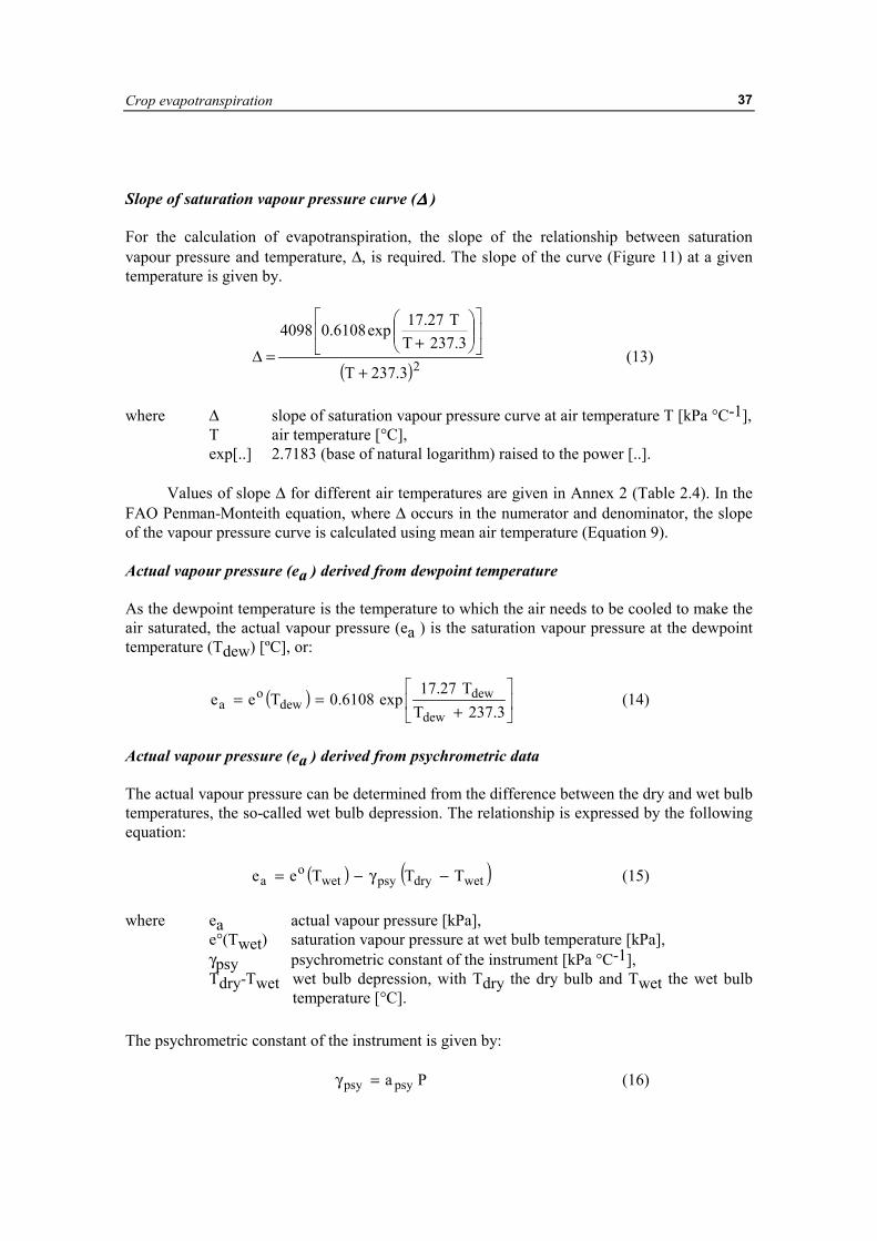
Crop evapotranspiration
37
Slope of saturation vapour pressure curve (∆∆∆∆ ) For the calculation of evapotranspiration, the slope of the relationship between saturation vapour pressure and temperature, ∆, is required. The slope of the curve (Figure 11) at a given temperature is given by.
( )23.237T
3.237TT27.17exp6108.04098
+
��
���
����
�
�
+=∆ (13)
where ∆ slope of saturation vapour pressure curve at air temperature T [kPa °C-1], T air temperature [°C], exp[..] 2.7183 (base of natural logarithm) raised to the power [..].
Values of slope ∆ for different air temperatures are given in Annex 2 (Table 2.4). In the FAO Penman-Monteith equation, where ∆ occurs in the numerator and denominator, the slope of the vapour pressure curve is calculated using mean air temperature (Equation 9). Actual vapour pressure (ea ) derived from dewpoint temperature As the dewpoint temperature is the temperature to which the air needs to be cooled to make the air saturated, the actual vapour pressure (ea ) is the saturation vapour pressure at the dewpoint temperature (Tdew) [ºC], or:
( ) ��
���
�
+==
3.237TT27.17
exp6108.0Teedew
dewdew
oa (14)
Actual vapour pressure (ea ) derived from psychrometric data The actual vapour pressure can be determined from the difference between the dry and wet bulb temperatures, the so-called wet bulb depression. The relationship is expressed by the following equation: ( ) ( )wetdrypsywet
oa TTTee −γ−= (15)
where ea actual vapour pressure [kPa], e°(Twet) saturation vapour pressure at wet bulb temperature [kPa], γpsy psychrometric constant of the instrument [kPa °C-1], Tdry-Twet wet bulb depression, with Tdry the dry bulb and Twet the wet bulb
temperature [°C].
The psychrometric constant of the instrument is given by: Pa psypsy =γ (16)
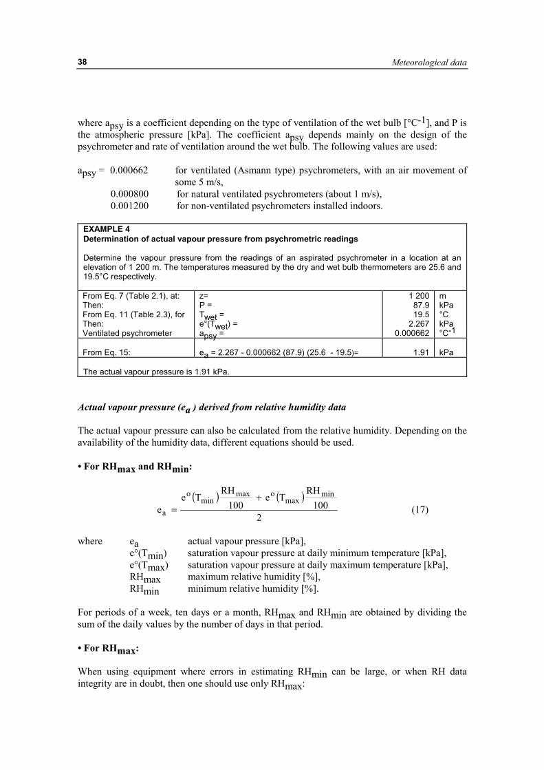
Meteorological data
38
where apsy is a coefficient depending on the type of ventilation of the wet bulb [°C-1], and P is the atmospheric pressure [kPa]. The coefficient apsy depends mainly on the design of the psychrometer and rate of ventilation around the wet bulb. The following values are used: apsy = 0.000662 for ventilated (Asmann type) psychrometers, with an air movement of
some 5 m/s, 0.000800 for natural ventilated psychrometers (about 1 m/s), 0.001200 for non-ventilated psychrometers installed indoors.
EXAMPLE 4 Determination of actual vapour pressure from psychrometric readings Determine the vapour pressure from the readings of an aspirated psychrometer in a location at an elevation of 1 200 m. The temperatures measured by the dry and wet bulb thermometers are 25.6 and 19.5°C respectively. From Eq. 7 (Table 2.1), at: Then:
z= P =
1 200 87.9
m kPa
From Eq. 11 (Table 2.3), for Then:
Twet = e°(Twet) =
19.5 2.267
°C kPa
Ventilated psychrometer apsy = 0.000662 °C-1 From Eq. 15:
ea = 2.267 - 0.000662 (87.9) (25.6 - 19.5)=
1.91
kPa
The actual vapour pressure is 1.91 kPa.
Actual vapour pressure (ea ) derived from relative humidity data The actual vapour pressure can also be calculated from the relative humidity. Depending on the availability of the humidity data, different equations should be used. • For RHmax and RHmin:
( ) ( )
2100
RHTe
100RH
Tee
minmax
omaxmin
o
a
+= (17)
where ea actual vapour pressure [kPa],
e°(Tmin) saturation vapour pressure at daily minimum temperature [kPa], e°(Tmax) saturation vapour pressure at daily maximum temperature [kPa], RHmax maximum relative humidity [%], RHmin minimum relative humidity [%].
For periods of a week, ten days or a month, RHmax and RHmin are obtained by dividing the sum of the daily values by the number of days in that period. • For RHmax: When using equipment where errors in estimating RHmin can be large, or when RH data integrity are in doubt, then one should use only RHmax:
Crop evapotranspiration
39
( )100
RHTee max
mino
a = (18)
• For RHmean: In the absence of RHmax and RHmin, another equation can be used to estimate ea:
( ) ( )
���
�
���
� +=
2TeTe
100RH
e mino
maxo
meana (19)
where RHmean is the mean relative humidity, defined as the average between RHmax and RHmin. However, Equation 19 is less desirable than are Equations 17 or 18.
EXAMPLE 5 Determination of actual vapour pressure from relative humidity Given the following daily minimum and maximum air temperature and the corresponding relative humidity data: Tmin = 18°C and RHmax = 82% Tmax = 25°C and RHmin = 54% Determine the actual vapour pressure. From Eq. 11 (Table 2.3), at: Then:
Tmin = e°(Tmin) =
18 2.064
°C kPa
From Eq. 11 (Table 2.3), at: Then:
Tmax = e°(Tmax) =
25 3.168
°C kPa
From Eq. 17: Note that when using Eq. 19:
ea = [2.064 (82/100) + 3.168 (54/100)] = ea =
1.70
1.78
kPa kPa
Vapour pressure deficit (es - ea )
The vapour pressure deficit is the difference between the saturation (es) and actual vapour pressure (ea) for a given time period. For time periods such as a week, ten days or a month es is computed from Equation 12 using the Tmax and Tmin averaged over the time period and similarly the ea is computed with one of the equations 4 to 19, using avrage measurements over the period. As stated above, using mean air temperature and not Tmax and Tmin in Equation 12 results in a lower estimate of es, thus in a lower vapour pressure deficit and hence an underestimation of the ETo (see Box 7). When desired, es and ea for long time periods cal also be calculated as averages of values computed for each day of the period.
EXAMPLE 6 Determination of vapour pressure deficit Determine the vapour pressure deficit with the data of the previous example (Example 5). From Example 5: e°(Tmin) =
e°(Tmax) = ea = es - ea = (2.064 + 3.168)/2 - 1.70 =
2.064 3.168
1.70 0.91
kPa kPa kPa kPa
The vapour pressure deficit is 0.91 kPa.
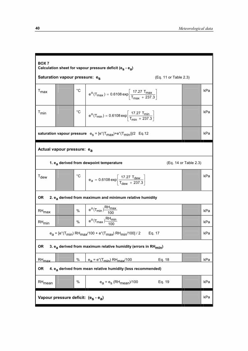
Meteorological data
40
BOX 7 Calculation sheet for vapour pressure deficit (es - ea) Saturation vapour pressure: es (Eq. 11 or Table 2.3) Tmax
°C
��
���
�
+=
3.237TT27.17
exp6108.0)T(emax
maxmax
o
kPa
Tmin
°C
��
���
�
+=
3.237TT27.17exp6108.0)T(e
minmin
mino
kPa
saturation vapour pressure es = [e°(Tmax)+e°(Tmin)]/2 Eq.12
kPa
Actual vapour pressure: ea 1. ea derived from dewpoint temperature (Eq. 14 or Table 2.3) Tdew
°C
��
���
�
+=
3.237TT27.17
exp6108.0edew
dewa
kPa
OR 2. ea derived from maximum and minimum relative humidity RHmax
% ( )
100RH
Te maxmin
o
kPa
RHmin
% ( )
100RH
Te minmax
o
kPa
ea = [e°(Tmin) RHmax/100 + e°(Tmax) RHmin/100] / 2 Eq. 17
kPa
OR 3. ea derived from maximum relative humidity (errors in RHmin) RHmax
%
ea = e°(Tmin) RHmax/100 Eq. 18
kPa
OR 4. ea derived from mean relative humidity (less recommended) RHmean
%
ea = es (RHmean)/100 Eq. 19
kPa
Vapour pressure deficit: (es - ea)
kPa
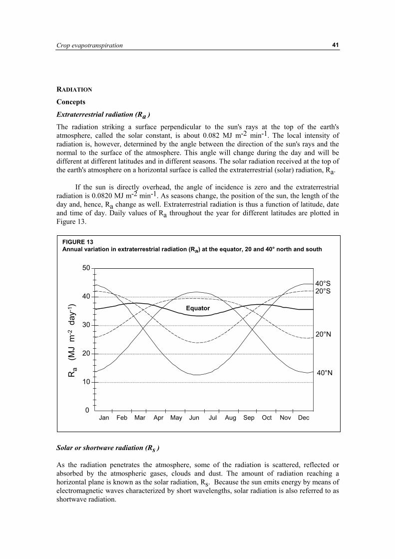
Crop evapotranspiration
41
RADIATION
Concepts
Extraterrestrial radiation (Ra )
The radiation striking a surface perpendicular to the sun's rays at the top of the earth's atmosphere, called the solar constant, is about 0.082 MJ m-2 min-1. The local intensity of radiation is, however, determined by the angle between the direction of the sun's rays and the normal to the surface of the atmosphere. This angle will change during the day and will be different at different latitudes and in different seasons. The solar radiation received at the top of the earth's atmosphere on a horizontal surface is called the extraterrestrial (solar) radiation, Ra.
If the sun is directly overhead, the angle of incidence is zero and the extraterrestrial radiation is 0.0820 MJ m-2 min-1. As seasons change, the position of the sun, the length of the day and, hence, Ra change as well. Extraterrestrial radiation is thus a function of latitude, date and time of day. Daily values of Ra throughout the year for different latitudes are plotted in Figure 13.
Solar or shortwave radiation (Rs ) As the radiation penetrates the atmosphere, some of the radiation is scattered, reflected or absorbed by the atmospheric gases, clouds and dust. The amount of radiation reaching a horizontal plane is known as the solar radiation, Rs. Because the sun emits energy by means of electromagnetic waves characterized by short wavelengths, solar radiation is also referred to as shortwave radiation.
FIGURE 13 Annual variation in extraterrestrial radiation (Ra) at the equator, 20 and 40° north and south
0
10
20
30
40
50
Ra
(M
J m
-2
day-
1 )
Jan Feb Mar Apr May Jun Jul Aug Sep Oct Nov Dec
40°S20°S
20°N
40°N
Equator

Meteorological data
42
For a cloudless day, Rs is roughly 75% of extraterrestrial radiation. On a cloudy day, the radiation is scattered in the atmosphere, but even with extremely dense cloud cover, about 25% of the extraterrestrial radiation may still reach the earth's surface mainly as diffuse sky radiation. Solar radiation is also known as global radiation, meaning that it is the sum of direct shortwave radiation from the sun and diffuse sky radiation from all upward angles. Relative shortwave radiation (Rs /Rso )
The relative shortwave radiation is the ratio of the solar radiation (Rs) to the clear-sky solar radiation (Rso). Rs is the solar radiation that actually reaches the earth's surface in a given period, while Rso is the solar radiation that would reach the same surface during the same period but under cloudless conditions.
The relative shortwave radiation is a way to express the cloudiness of the atmosphere; the cloudier the sky the smaller the ratio. The ratio varies between about 0.33 (dense cloud cover) and 1 (clear sky). In the absence of a direct measurement of Rn, the relative shortwave radiation is used in the computation of the net longwave radiation.
Relative sunshine duration (n/N)
The relative sunshine duration is another ratio that expresses the cloudiness of the atmosphere. It is the ratio of the actual duration of sunshine, n, to the maximum possible duration of sunshine or daylight hours N. In the absence of any clouds, the actual duration of sunshine is equal to the daylight hours (n = N) and the ratio is one, while on cloudy days n and consequently the ratio may be zero. In the absence of a direct measurement of Rs, the relative sunshine duration, n/N, is often used to derive solar radiation from extraterrestrial radiation.
As with extraterrestrial radiation, the daylength N depends on the position of the sun and is hence a function of latitude and date. Daily values of N throughout the year for different latitudes are plotted in Figure 14.
FIGURE 14 Annual variation of the daylight hours (N) at the equator, 20 and 40° north and south
40 S
20 S
20 N
40 N
o
o
o
o
8
9
10
11
12
13
14
15
16
N d
aylig
ht h
ours
(
hour
s/da
y)
Equator
Jan Feb Mar Apr May Jun Jul Aug Sep Oct Nov Dec
Crop evapotranspiration
43
Albedo (αααα) and net solar radiation (Rns)
A considerable amount of solar radiation reaching the earth's surface is reflected. The fraction, α, of the solar radiation reflected by the surface is known as the albedo. The albedo is highly variable for different surfaces and for the angle of incidence or slope of the ground surface. It may be as large as 0.95 for freshly fallen snow and as small as 0.05 for a wet bare soil. A green vegetation cover has an albedo of about 0.20-0.25. For the green grass reference crop, α is assumed to have a value of 0.23.
The net solar radiation, Rns, is the fraction of the solar radiation Rs that is not reflected from the surface. Its value is (1-α)Rs. Net longwave radiation (Rnl)
The solar radiation absorbed by the earth is converted to heat energy. By several processes, including emission of radiation, the earth loses this energy. The earth, which is at a much lower temperature than the sun, emits radiative energy with wavelengths longer than those from the sun. Therefore, the terrestrial radiation is referred to as longwave radiation. The emitted longwave radiation (Rl,up) is absorbed by the atmosphere or is lost into space. The longwave radiation received by the atmosphere (Rl,down) increases its temperature and, as a consequence, the atmosphere radiates energy of its own, as illustrated in Figure 15. Part of the radiation finds it way back to the earth's surface. Consequently, the earth's surface both emits and receives longwave radiation. The difference between outgoing and incoming longwave radiation is called the net longwave radiation, Rnl. As the outgoing longwave radiation is almost always greater than the incoming longwave radiation, Rnl represents an energy loss. Net radiation (Rn)
The net radiation, Rn, is the difference between incoming and outgoing radiation of both short and long wavelengths. It is the balance between the energy absorbed, reflected and emitted by the earth's surface or the difference between the incoming net shortwave (Rns) and the net outgoing longwave (Rnl) radiation (Figure 15). Rn is normally positive during the daytime and negative during the nighttime. The total daily value for Rn is almost always positive over a period of 24 hours, except in extreme conditions at high latitudes. Soil heat flux (G)
In making estimates of evapotranspiration, all terms of the energy balance (Equation 1) should be considered. The soil heat flux, G, is the energy that is utilized in heating the soil. G is positive when the soil is warming and negative when the soil is cooling. Although the soil heat flux is small compared to Rn and may often be ignored, the amount of energy gained or lost by the soil in this process should theoretically be subtracted or added to Rn when estimating evapotranspiration. Units
The standard unit used in this handbook to express energy received on a unit surface per unit time is megajoules per square metre per day (MJ m-2 day-1). In meteorological bulletins other units might be used or radiation might even be expressed in units no longer accepted as standard S.I. units, such as calories cm-2 day-1.
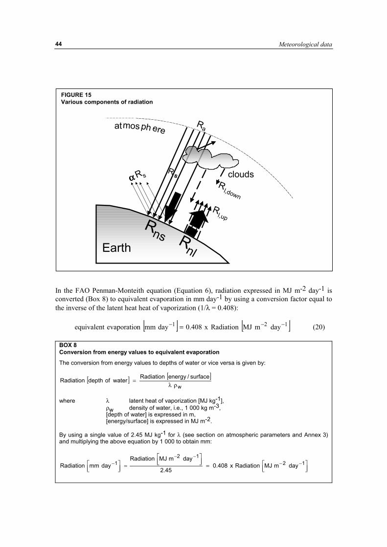
Meteorological data
44
In the FAO Penman-Monteith equation (Equation 6), radiation expressed in MJ m-2 day-1 is converted (Box 8) to equivalent evaporation in mm day-1 by using a conversion factor equal to the inverse of the latent heat heat of vaporization (1/λ = 0.408): [ ] [ ]121 daymMJRadiationx408.0daymmnevaporatioequivalent −−− = (20)
BOX 8 Conversion from energy values to equivalent evaporation The conversion from energy values to depths of water or vice versa is given by:
[ ] [ ]w
surface/energyRadiationwaterofdepthRadiationρλ
=
where λ latent heat of vaporization [MJ kg-1],
ρw density of water, i.e., 1 000 kg m-3, [depth of water] is expressed in m, [energy/surface] is expressed in MJ m-2.
By using a single value of 2.45 MJ kg-1 for λ (see section on atmospheric parameters and Annex 3) and multiplying the above equation by 1 000 to obtain mm:
���
���=
���
���
≈���
��� −−
−−− 12
121 daymMJRadiationx408.0
45.2
daymMJRadiationdaymmRadiation
FIGURE 15 Various components of radiation
clouds
Earth
atmosph ere
RsRs
Ra
R
R
l,down
l,upRns Rnl
αααα
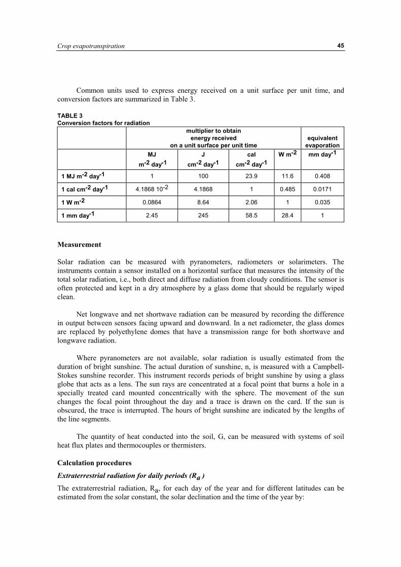
Crop evapotranspiration
45
Common units used to express energy received on a unit surface per unit time, and conversion factors are summarized in Table 3. TABLE 3 Conversion factors for radiation
multiplier to obtain energy received
on a unit surface per unit time
equivalent
evaporation MJ
m-2 day-1 J
cm-2 day-1 cal
cm-2 day-1 W m-2 mm day-1
1 MJ m-2 day-1 1 100 23.9 11.6 0.408
1 cal cm-2 day-1 4.1868 10-2 4.1868 1 0.485 0.0171
1 W m-2 0.0864 8.64 2.06 1 0.035
1 mm day-1 2.45 245 58.5 28.4 1
Measurement Solar radiation can be measured with pyranometers, radiometers or solarimeters. The instruments contain a sensor installed on a horizontal surface that measures the intensity of the total solar radiation, i.e., both direct and diffuse radiation from cloudy conditions. The sensor is often protected and kept in a dry atmosphere by a glass dome that should be regularly wiped clean.
Net longwave and net shortwave radiation can be measured by recording the difference in output between sensors facing upward and downward. In a net radiometer, the glass domes are replaced by polyethylene domes that have a transmission range for both shortwave and longwave radiation.
Where pyranometers are not available, solar radiation is usually estimated from the duration of bright sunshine. The actual duration of sunshine, n, is measured with a Campbell-Stokes sunshine recorder. This instrument records periods of bright sunshine by using a glass globe that acts as a lens. The sun rays are concentrated at a focal point that burns a hole in a specially treated card mounted concentrically with the sphere. The movement of the sun changes the focal point throughout the day and a trace is drawn on the card. If the sun is obscured, the trace is interrupted. The hours of bright sunshine are indicated by the lengths of the line segments.
The quantity of heat conducted into the soil, G, can be measured with systems of soil heat flux plates and thermocouples or thermisters. Calculation procedures
Extraterrestrial radiation for daily periods (Ra )
The extraterrestrial radiation, Ra, for each day of the year and for different latitudes can be estimated from the solar constant, the solar declination and the time of the year by:
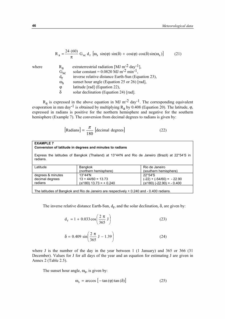
Meteorological data
46
[ ])sin()cos()cos()sin()sin(dG)60(24R ssrsca ωδϕ+δϕωπ
= (21)
where Ra extraterrestrial radiation [MJ m-2 day-1],
Gsc solar constant = 0.0820 MJ m-2 min-1, dr inverse relative distance Earth-Sun (Equation 23), ωs sunset hour angle (Equation 25 or 26) [rad], ϕ latitude [rad] (Equation 22), δ solar declination (Equation 24) [rad].
Ra is expressed in the above equation in MJ m-2 day-1. The corresponding equivalent
evaporation in mm day-1 is obtained by multiplying Ra by 0.408 (Equation 20). The latitude, ϕ, expressed in radians is positive for the northern hemisphere and negative for the southern hemisphere (Example 7). The conversion from decimal degrees to radians is given by:
[ ] [ ]degreesdecimalRadians180π= (22)
EXAMPLE 7 Conversion of latitude in degrees and minutes to radians Express the latitudes of Bangkok (Thailand) at 13°44'N and Rio de Janeiro (Brazil) at 22°54’S in radians. Latitude Bangkok
(northern hemisphere) Rio de Janeiro (southern hemisphere)
degrees & minutes decimal degrees radians
13°44'N 13 + 44/60 = 13.73 (π/180) 13.73 = + 0.240
22°54'S (-22) + (-54/60) = - 22.90 (π/180) (-22.90) = - 0.400
The latitudes of Bangkok and Rio de Janeiro are respectively + 0.240 and - 0.400 radians.
The inverse relative distance Earth-Sun, dr, and the solar declination, δ, are given by:
��
���
� π+= J
3652cos033.01dr (23)
��
���
� −π
=δ 39.1J3652sin409.0 (24)
where J is the number of the day in the year between 1 (1 January) and 365 or 366 (31 December). Values for J for all days of the year and an equation for estimating J are given in Annex 2 (Table 2.5).
The sunset hour angle, ωs, is given by: [ ])(tan)(tanarccoss δϕ−=ω (25)
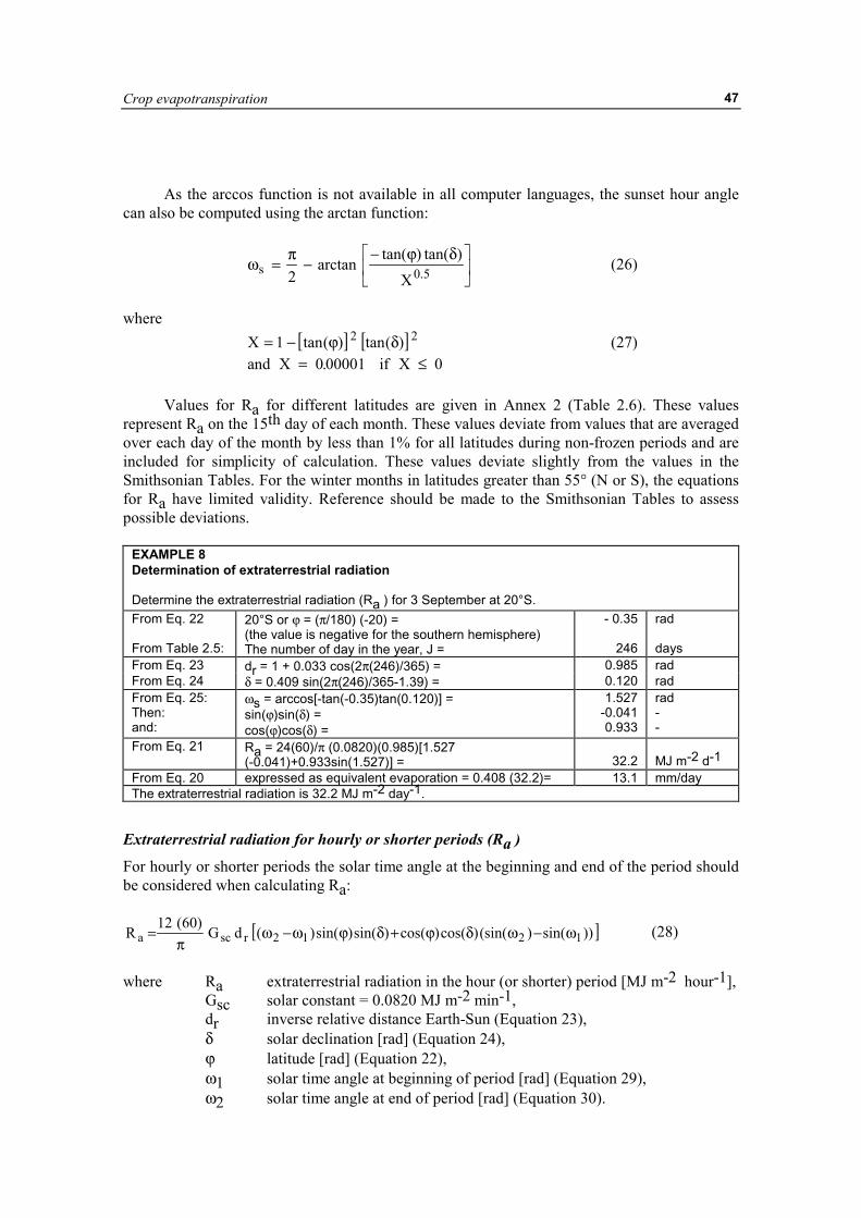
Crop evapotranspiration
47
As the arccos function is not available in all computer languages, the sunset hour angle can also be computed using the arctan function:
��
���
� δϕ−−π=ω 5.0s
X
)tan()tan(arctan2
(26)
where [ ] [ ] 22 )(tan)(tan1X δϕ−= (27) and X if X= ≤0 00001 0.
Values for Ra for different latitudes are given in Annex 2 (Table 2.6). These values represent Ra on the 15th day of each month. These values deviate from values that are averaged over each day of the month by less than 1% for all latitudes during non-frozen periods and are included for simplicity of calculation. These values deviate slightly from the values in the Smithsonian Tables. For the winter months in latitudes greater than 55° (N or S), the equations for Ra have limited validity. Reference should be made to the Smithsonian Tables to assess possible deviations.
EXAMPLE 8 Determination of extraterrestrial radiation Determine the extraterrestrial radiation (Ra ) for 3 September at 20°S. From Eq. 22 From Table 2.5:
20°S or ϕ = (π/180) (-20) = (the value is negative for the southern hemisphere) The number of day in the year, J =
- 0.35
246
rad days
From Eq. 23 dr = 1 + 0.033 cos(2π(246)/365) = 0.985 rad From Eq. 24 δ = 0.409 sin(2π(246)/365-1.39) = 0.120 rad From Eq. 25: Then: and:
ωs = arccos[-tan(-0.35)tan(0.120)] = sin(ϕ)sin(δ) = cos(ϕ)cos(δ) =
1.527 -0.041 0.933
rad - -
From Eq. 21 Ra = 24(60)/π (0.0820)(0.985)[1.527 (-0.041)+0.933sin(1.527)] =
32.2
MJ m-2 d-1
From Eq. 20 expressed as equivalent evaporation = 0.408 (32.2)= 13.1 mm/day The extraterrestrial radiation is 32.2 MJ m-2 day-1.
Extraterrestrial radiation for hourly or shorter periods (Ra )
For hourly or shorter periods the solar time angle at the beginning and end of the period should be considered when calculating Ra:
[ ]))sin()sin(()cos()cos()sin()sin()(dG)60(12
R 1212rsca ω−ωδϕ+δϕω−ωπ
= (28)
where Ra extraterrestrial radiation in the hour (or shorter) period [MJ m-2 hour-1],
Gsc solar constant = 0.0820 MJ m-2 min-1, dr inverse relative distance Earth-Sun (Equation 23), δ solar declination [rad] (Equation 24), ϕ latitude [rad] (Equation 22), ω1 solar time angle at beginning of period [rad] (Equation 29), ω2 solar time angle at end of period [rad] (Equation 30).

Meteorological data
48
The solar time angles at the beginning and end of the period are given by:
24
t11
π−ω=ω (29)
24
t12
π+ω=ω (30)
where ω solar time angle at midpoint of hourly or shorter period [rad],
tl length of the calculation period [hour]: i.e., 1 for hourly period or 0.5 for a 30-minute period.
The solar time angle at midpoint of the period is:
[ ]12)S)LL(06667.0t(12 cmz −+−+π
=ω (31)
where t standard clock time at the midpoint of the period [hour]. For example for a
period between 14.00 and 15.00 hours, t = 14.5, Lz longitude of the centre of the local time zone [degrees west of Greenwich].
For example, Lz = 75, 90, 105 and 120° for the Eastern, Central, Rocky Mountain and Pacific time zones (United States) and Lz = 0° for Greenwich, 330° for Cairo (Egypt), and 255° for Bangkok (Thailand),
Lm longitude of the measurement site [degrees west of Greenwich], Sc seasonal correction for solar time [hour].
Of course, ω < -ωs or ω > ωs from Equation 31 indicates that the sun is below the horizon so that, by definition, Ra is zero. The seasonal correction for solar time is: )bsin(025.0)bcos(1255.0)b2sin(1645.0Sc −−= (32)
bJ
=−2 81
364π ( )
(33)
where J is the number of the day in the year. Daylight hours (N) The daylight hours, N, are given by:
s24N ωπ
= (34)
where ωs is the sunset hour angle in radians given by Equation 25 or 26. Mean values for N (15th day of each month) for different latitudes are given in Annex 2, Table 2.7.
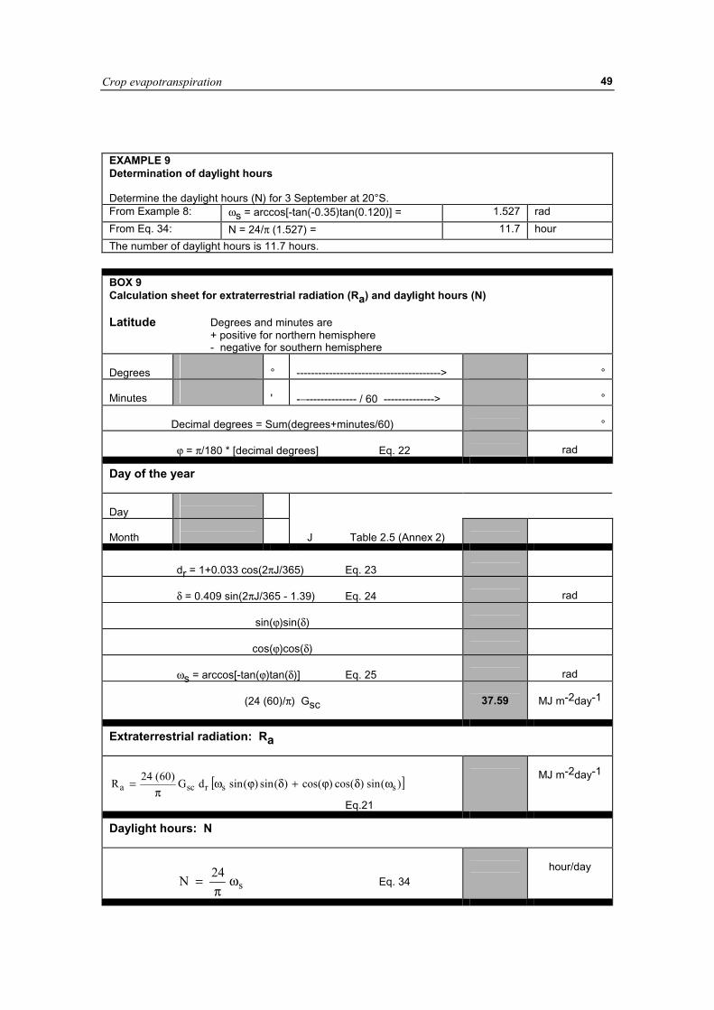
Crop evapotranspiration
49
EXAMPLE 9 Determination of daylight hours Determine the daylight hours (N) for 3 September at 20°S. From Example 8: ωs = arccos[-tan(-0.35)tan(0.120)] = 1.527 rad From Eq. 34: N = 24/π (1.527) = 11.7 hour The number of daylight hours is 11.7 hours.
BOX 9 Calculation sheet for extraterrestrial radiation (Ra) and daylight hours (N) Latitude Degrees and minutes are + positive for northern hemisphere - negative for southern hemisphere Degrees
°
---------------------------------------->
°
Minutes
'
-−-------------- / 60 -------------->
°
Decimal degrees = Sum(degrees+minutes/60)
°
ϕ = π/180 * [decimal degrees] Eq. 22
rad
Day of the year Day
Month
J Table 2.5 (Annex 2)
dr = 1+0.033 cos(2πJ/365) Eq. 23
δ = 0.409 sin(2πJ/365 - 1.39) Eq. 24
rad
sin(ϕ)sin(δ)
cos(ϕ)cos(δ)
ωs = arccos[-tan(ϕ)tan(δ)] Eq. 25
rad
(24 (60)/π) Gsc
37.59
MJ m-2day-1
Extraterrestrial radiation: Ra
[ ])(sin)(cos)(cos)(sin)(sindG)60(24R ssrsca ωδϕ+δϕωπ
=
Eq.21
MJ m-2day-1
Daylight hours: N
s24N ωπ
= Eq. 34
hour/day
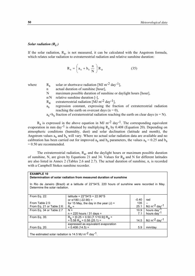
Meteorological data
50
Solar radiation (Rs ) If the solar radiation, Rs, is not measured, it can be calculated with the Angstrom formula, which relates solar radiation to extraterrestrial radiation and relative sunshine duration:
where Rs solar or shortwave radiation [MJ m-2 day-1], n actual duration of sunshine [hour], N maximum possible duration of sunshine or daylight hours [hour], n/N relative sunshine duration [-], Ra extraterrestrial radiation [MJ m-2 day-1], as regression constant, expressing the fraction of extraterrestrial radiation
reaching the earth on overcast days (n = 0), as+bs fraction of extraterrestrial radiation reaching the earth on clear days (n = N). Rs is expressed in the above equation in MJ m-2 day-1. The corresponding equivalent evaporation in mm day-1 is obtained by multiplying Rs by 0.408 (Equation 20). Depending on atmospheric conditions (humidity, dust) and solar declination (latitude and month), the Angstrom values as and bs will vary. Where no actual solar radiation data are available and no calibration has been carried out for improved as and bs parameters, the values as = 0.25 and bs = 0.50 are recommended. The extraterrestrial radiation, Ra, and the daylight hours or maximum possible duration of sunshine, N, are given by Equations 21 and 34. Values for Ra and N for different latitudes are also listed in Annex 2 (Tables 2.6 and 2.7). The actual duration of sunshine, n, is recorded with a Campbell Stokes sunshine recorder.
EXAMPLE 10 Determination of solar radiation from measured duration of sunshine In Rio de Janeiro (Brazil) at a latitude of 22°54’S, 220 hours of sunshine were recorded in May. Determine the solar radiation. From Eq. 22: From Table 2.5: From Eq. 21 or Table 2.6:
latitude = 22°54’S = 22.90°S or π/180 (-22.90) = for 15 May, the day in the year (J) = Ra =
-0.40
135 25.1
rad -- MJ m-2 day-1
From Eq. 34 or Table 2.7 N = n = 220 hours / 31 days =
10.9 7.1
hours day-1 hours day-1
From Eq. 35:
Rs = [0.25 + 0.50 (7.1/10.9)] Ra = = 0.58 Ra = 0.58 (25.1) =
14.5
MJ m-2 day-1
From Eq. 20:
expressed as equivalent evaporation = 0.408 (14.5) =
5.9
mm/day
The estimated solar radiation is 14.5 MJ m-2 day-1.
asss RNnbaR �
�
���
� += (35)
Crop evapotranspiration
51
Clear-sky solar radiation (Rso ) The calculation of the clear-sky radiation, Rso, when n = N, is required for computing net longwave radiation. • For near sea level or when calibrated values for as and bs are available:
where Rso clear-sky solar radiation [MJ m-2 day-1], as+bs fraction of extraterrestrial radiation reaching the earth on clear-sky days (n = N). • When calibrated values for as and bs are not available:
where z station elevation above sea level [m]. Other more complex estimates for Rso, which include turbidity and water vapour effects, are discussed in Annex 3 (Equations 3.14 to 20). Net solar or net shortwave radiation (Rns ) The net shortwave radiation resulting from the balance between incoming and reflected solar radiation is given by: sns R)1(R α−= (38) where Rns net solar or shortwave radiation [MJ m-2 day-1],
α albedo or canopy reflection coefficient, which is 0.23 for the hypothetical grass reference crop [dimensionless],
Rs the incoming solar radiation [MJ m-2 day-1]. Rns is expressed in the above equation in MJ m-2 day-1. Net longwave radiation (Rnl ) The rate of longwave energy emission is proportional to the absolute temperature of the surface raised to the fourth power. This relation is expressed quantitatively by the Stefan-Boltzmann law. The net energy flux leaving the earth's surface is, however, less than that emitted and given by the Stefan-Boltzmann law due to the absorption and downward radiation from the sky. Water vapour, clouds, carbon dioxide and dust are absorbers and emitters of longwave radiation. Their concentrations should be known when assessing the net outgoing flux. As humidity and cloudiness play an important role, the Stefan-Boltzmann law is corrected by these two factors when estimating the net outgoing flux of longwave radiation. It is thereby assumed that the concentrations of the other absorbers are constant:
assso R)ba(R += (36)
( ) a5
so Rz10275.0R −+= (37)

Meteorological data
52
where Rnl net outgoing longwave radiation [MJ m-2 day-1], σ Stefan-Boltzmann constant [ 4.903 10-9 MJ K-4 m-2 day-1], Tmax,K maximum absolute temperature during the 24-hour period [K = °C + 273.16], Tmin,K minimum absolute temperature during the 24-hour period [K = °C + 273.16], ea actual vapour pressure [kPa], Rs/Rso relative shortwave radiation (limited to ≤ 1.0), Rs measured or calculated (Equation 35) solar radiation [MJ m-2 day-1], Rso calculated (Equation 36 or 37) clear-sky radiation [MJ m-2 day-1].
An average of the maximum air temperature to the fourth power and the minimum air temperature to the fourth power is commonly used in the Stefan-Boltzmann equation for 24-hour time steps. The term (0.34-0.14√ea) expresses the correction for air humidity, and will be smaller if the humidity increases. The effect of cloudiness is expressed by (1.35 Rs/Rso - 0.35). The term becomes smaller if the cloudiness increases and hence Rs decreases. The smaller the correction terms, the smaller the net outgoing flux of longwave radiation. Note that the Rs/Rso term in Equation 39 must be limited so that Rs/Rso ≤ 1.0. Where measurements of incoming and outgoing short and longwave radiation during bright sunny and overcast hours are available, calibration of the coefficients in Equation 39 can be carried out. Annex 2 (Table 2.8) lists values for σTK4 for different air temperatures.
EXAMPLE 11 Determination of net longwave radiation In Rio de Janeiro (Brazil) at a latitude of 22°54’S (= -22.70°), 220 hours of bright sunshine, a mean monthly daily maximum and minimum air temperature of 25.1 and 19.1°C and a vapour pressure of 2.1 kPa were recorded in May. Determine the net longwave radiation. From Example 10: Rs = 14.5 MJ m-2 day-1 From Eq. 36: Rso = 0.75 Ra = 0.75 . 25.1 = 18.8 MJ m-2 day-1 From Table 2.8 or for: Then: and:
σ = Tmax = 25.1°C = σTmax,K4 =
4.903 10-9 298.3
38.8
MJ K-4 m-2 day-1 K MJ m-2 day-1
and: and:
Tmin = 19.1°C = σ Tmin,K4 = 35.8 MJ m-2 day-1
292.3 35.8
K MJ m-2 day-1
and: and:
ea = 0.34 - 0.14 √ea =
2.1 0.14
kPa -
and: -
Rs/Rso = (14.5)/(18.8) 1.35(0.77)-0.35 =
0.77 0.69
- -
From Eq. 39: Rnl = [(38.7 + 35.7)/2] (0.14) (0.69) = 3.5 MJ m-2 day-1 From Eq. 20: expressed as equivalent evaporation =
0.408 (3.5) =
1.4 mm/day
The net longwave radiation is 3.5 MJ m-2 day-1.
( ) ���
����
�−−
��
�
�
� +σ= 35.0
RR
35.1e14.034.02
TTR
so
sa
4K,min
4K,max
nl (39)
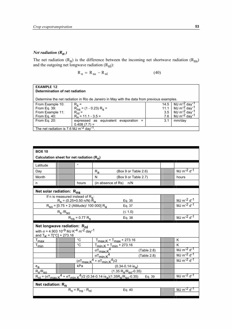
Crop evapotranspiration
53
Net radiation (Rn )
The net radiation (Rn) is the difference between the incoming net shortwave radiation (Rns) and the outgoing net longwave radiation (Rnl):
nlnsn RRR −= (40)
EXAMPLE 12 Determination of net radiation Determine the net radiation in Rio de Janeiro in May with the data from previous examples. From Example 10: Rs = 14.5 MJ m-2 day-1 From Eq. 39: Rns = (1 - 0.23) Rs = 11.1 MJ m-2 day-1 From Example 11: Rnl = 3.5 MJ m-2 day-1 From Eq. 40: Rn = 11.1 - 3.5 = 7.6 MJ m-2 day-1 From Eq. 20: expressed as equivalent evaporation =
0.408 (7.7) = 3.1 mm/day
The net radiation is 7.6 MJ m-2 day-1.
BOX 10 Calculation sheet for net radiation (Rn)
Latitude ° Day Ra (Box 9 or Table 2.6) MJ m-2 d-1 Month N (Box 9 or Table 2.7) hours n hours (in absence of Rs) n/N
Net solar radiation: Rns If n is measured instead of Rs: Rs = (0.25+0.50 n/N) Ra Eq. 35
MJ m-2 d-1
Rso = [0.75 + 2 (Altitude)/ 100 000] Ra Eq. 37 MJ m-2 d-1
Rs /Rso (≤ 1.0)
Rns = 0.77 Rs Eq. 38 MJ m-2 d-1
Net longwave radiation: Rnl with σ = 4.903 10-9 MJ K-4 m-2 day-1 and TK = T[°C] + 273.16 Tmax °C Tmax,K = Tmax + 273.16 K Tmin °C Tmin,K = Tmin + 273.16 K σTmax,K4 (Table 2.8) MJ m-2 d-1 σTmin,K4 (Table 2.8) MJ m-2 d-1
(σTmax,K4 + σTmin,K4)/2 MJ m-2 d-1 ea kPa (0.34-0.14√ea) Rs/Rso (1.35 Rs/Rso-0.35) Rnl = (σTmax,K4 + σTmin,K4)/2 (0.34-0.14√ea)(1.35Rs/Rso-0.35) Eq. 39 MJ m-2 d-1
Net radiation: Rn MJ m-2 d-1 Rn = Rns - Rnl Eq. 40
Meteorological data
54
Soil heat flux (G)
Complex models are available to describe soil heat flux. Because soil heat flux is small compared to Rn, particularly when the surface is covered by vegetation and calculation time steps are 24 hours or longer, a simple calculation procedure is presented here for long time steps, based on the idea that the soil temperature follows air temperature:
where G soil heat flux [MJ m-2 day-1], cs soil heat capacity [MJ m-3 °C-1], Ti air temperature at time i [°C], Ti-1 air temperature at time i-1 [°C], ∆t length of time interval [day], ∆z effective soil depth [m]. As the soil temperature lags air temperature, the average temperature for a period should be considered when assessing the daily soil heat flux, i.e., ∆t should exceed one day. The depth of penetration of the temperature wave is determined by the length of the time interval. The effective soil depth, ∆z, is only 0.10-0.20 m for a time interval of one or a few days but might be 2 m or more for monthly periods. The soil heat capacity is related to its mineral composition and water content. • For day and ten-day periods: As the magnitude of the day or ten-day soil heat flux beneath the grass reference surface is relatively small, it may be ignored and thus:
• For monthly periods: When assuming a constant soil heat capacity of 2.1 MJ m-3 °C-1 and an appropriate soil depth, Equation 41 can be used to derive G for monthly periods:
or, if Tmonth,i+1 is unknown:
where Tmonth,i mean air temperature of month i [°C],
Tmonth,i-1 mean air temperature of previous month [°C], Tmonth,i+1 mean air temperature of next month [°C].
• For hourly or shorter periods: For hourly (or shorter) calculations, G beneath a dense cover of grass does not correlate well with air temperature. Hourly G can be approximated during daylight periods as:
ztTT
cG 1iis ∆
∆
+= − (41)
0Gday ≈ (42)
)TT(07.0G 1i,month1i,monthi,month −+ −= (43)
)TT(14.0G 1i,monthi,monthi,month −−= (44)
Crop evapotranspiration
55
and during nighttime periods as:
Where the soil is warming, the soil heat flux G is positive. The amount of energy required for this process is subtracted from Rn when estimating evapotranspiration.
EXAMPLE 13 Determination of soil heat flux for monthly periods Determine the soil heat flux in April in Algiers (Algeria) when the soil is warming. The mean monthly temperatures of March, April and May are 14.1, 16.1, and 18.8°C respectively. From Eq. 43
for the month of April: Gmonth = 0.07 (18.8 - 14.1) =
0.33
MJ m-2 day-1
From Eq. 20
expressed as equivalent evaporation = 0.408(0.33) =
0.13
mm/day
The soil heat flux is 0.33 MJ m-2 day-1.
WIND SPEED Measurement Wind is characterized by its direction and velocity. Wind direction refers to the direction from which the wind is blowing. For the computation of evapotranspiration, wind speed is the relevant variable. As wind speed at a given location varies with time, it is necessary to express it as an average over a given time interval. Wind speed is given in metres per second (m s-1) or kilometres per day (km day-1). Wind speed is measured with anemometers. The anemometers commonly used in weather stations are composed of cups or propellers which are turned by the force of the wind. By counting the number of revolutions over a given time period, the average wind speed over the measuring period is computed. Wind profile relationship Wind speeds measured at different heights above the soil surface are different. Surface friction tends to slow down wind passing over it. Wind speed is slowest at the surface and increases with height. For this reason anemometers are placed at a chosen standard height, i.e., 10 m in meteorology and 2 or 3 m in agrometeorology. For the calculation of evapotranspiration, wind speed measured at 2 m above the surface is required. To adjust wind speed data obtained from instruments placed at elevations other than the standard height of 2 m, a logarithmic wind speed profile may be used for measurements above a short grassed surface:
nhr R1.0G = (45)
nhr R5.0G = (46)
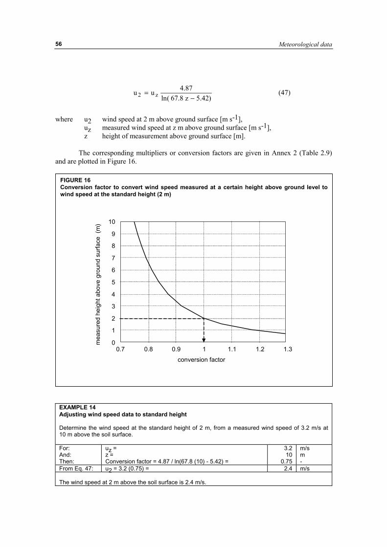
Meteorological data
56
where u2 wind speed at 2 m above ground surface [m s-1],
uz measured wind speed at z m above ground surface [m s-1], z height of measurement above ground surface [m].
The corresponding multipliers or conversion factors are given in Annex 2 (Table 2.9) and are plotted in Figure 16.
EXAMPLE 14 Adjusting wind speed data to standard height Determine the wind speed at the standard height of 2 m, from a measured wind speed of 3.2 m/s at 10 m above the soil surface. For: And: Then:
uz = z = Conversion factor = 4.87 / ln(67.8 (10) - 5.42) =
3.2 10
0.75
m/s m -
From Eq. 47: u2 = 3.2 (0.75) = 2.4 m/s The wind speed at 2 m above the soil surface is 2.4 m/s.
)42.5z8.67(ln
87.4uu z2 −= (47)
FIGURE 16 Conversion factor to convert wind speed measured at a certain height above ground level to wind speed at the standard height (2 m)
0
1
2
3
4
5
6
7
8
9
10
0.7 0.8 0.9 1 1.1 1.2 1.3conversion factor
mea
sure
d he
ight
abo
ve g
roun
d su
rface
(m
)
Crop evapotranspiration
57
CLIMATIC DATA ACQUISITION Weather stations Meteorological data are recorded at various types of weather stations. Agrometeorological stations are sited in cropped areas where instruments are exposed to atmospheric conditions similar to those for the surrounding crops. In these stations, air temperature and humidity, wind speed and sunshine duration are typically measured at 2 m above an extensive surface of grass or short crop. Where needed and feasible, the cover of the station is irrigated. Guidelines for the establishment and maintenance of agrometeorological stations are given in the FAO Irrigation and Drainage Paper No. 27. This handbook also describes the different types of instruments, their installation and reliability. Data collected at stations other than agrometeorological stations require a careful analysis of their validity before their use. For example, in aeronautic stations, data relevant for aviation are measured. As airports are often situated near urban conditions, temperatures may be higher than those found in rural agricultural areas. Wind speed is commonly measured at 10 m height above the ground surface. The country’s national meteorological service should be contacted for information on the climatic data collected at various types of weather stations in the country. National services commonly publish meteorological bulletins listing processed climatic data from the various stations. The annexes list procedures for the statistical analysis, assessment, correction and completion of partial or missing weather data: Annex 4: Statistical analysis of weather data sets; Annex 5: Measuring and assessing integrity of weather data; Annex 6: Correction of weather data observed at non-reference sites for computing ETo. Agroclimatic monthly databases Starting in 1984, FAO has published mean monthly agroclimatic data from 2 300 stations in the FAO Plant Production and Protection Series. Several volumes exist: No. 22: Volume 1: data for Africa, countries north of the equator (1984),
Volume 2: data for Africa, countries south of the equator (1984); No. 24: Agroclimatic data for Latin America and the Caribbean (1985); No. 25: Volume 1: Agroclimatic data for Asia (A-J) (1987),
Volume 2: Agroclimatic data for Asia (K-Z) (1987). CLIMWAT for CROPWAT (FAO Irrigation and Drainage Paper No. 46) contains monthly data from 3 262 climatic stations contained on five separate diskettes. The stations are grouped by country and by continent. Monthly averages of maximum and minimum temperatures, mean relative humidity, wind speed, sunshine hours, radiation data as well as rainfall and ETo calculated with the FAO Penman-Monteith method are listed on the diskettes for mean long-term conditions.
Meteorological data
58
FAOCLIM provides a user friendly interface on compact disc to the agroclimatic database of the Agrometeorology Group in FAO. The data presented are an extension of the previously published FAO Plant Production and Protection Series and the number of stations has been increased from 2 300 to about 19 000, with an improved world wide coverage. However, values for all principal weather parameters are not available for all stations. Many contain air temperature and precipitation only. These databases can be consulted in order to verify the consistency of the actual database or to estimate missing climatic parameters. However, they should only be used for preliminary studies as they contain mean monthly data only. FAOCLIM provides monthly time series for only a few stations. The information in these databases should never replace actual data. Other electronic databases for portions of the globe have been published by the International Water Management Institute (IWMI). These databases include daily and monthly air temperature, precipitation and ETo predicted using the Hargreaves ETo equation that is based on differences between daily maximum and minimum air temperature. ESTIMATING MISSING CLIMATIC DATA
The assessment of the reference evapotranspiration ETo with the Penman-Monteith method is developed in Chapter 4. The calculation requires mean daily, ten-day or monthly maximum and minimum air temperature (Tmax and Tmin), actual vapour pressure (ea), net radiation (Rn) and wind speed measured at 2 m (u2). If some of the required weather data are missing or cannot be calculated, it is strongly recommended that the user estimate the missing climatic data with one of the following procedures and use the FAO Penman-Monteith method for the calculation of ETo. The use of an alternative ETo calculation procedure, requiring only limited meteorological parameters, is less recommended. Procedures to estimate missing humidity, radiation and wind speed data are given in this section. Estimating missing humidity data
Where humidity data are lacking or are of questionable quality, an estimate of actual vapour pressure, ea, can be obtained by assuming that dewpoint temperature (Tdew) is near the daily minimum temperature (Tmin). This statement implicitly assumes that at sunrise, when the air temperature is close to Tmin, that the air is nearly saturated with water vapour and the relative humidity is nearly 100%. If Tmin is used to represent Tdew then:
��
���
�
+==
3.237TT27.17
exp611.0)T(eemin
minmin
oa (48)
The relationship Tdew ≈ Tmin holds for locations where the cover crop of the station is
well watered. However, particularly for arid regions, the air might not be saturated when its temperature is at its minimum. Hence, Tmin might be greater than Tdew and a further calibration may be required to estimate dewpoint temperatures. In these situations, “Tmin” in the above equation may be better approximated by subtracting 2-3°C from Tmin. Appropriate correction procedures are given in Annex 6. In humid and subhumid climates, Tmin and Tdew measured in early morning may be less than Tdew measured during the daytime because of condensation of dew during the night. After sunrise, evaporation of the dew will once again
Crop evapotranspiration
59
humidify the air and will increase the value measured for Tdew during the daytime. This phenomenon is demonstrated in Figure 5.4 of Annex 5. However, it is standard practice in 24-hour calculations of ETo to use Tdew measured or calculated durin early morning.
The estimate for ea from Tmin should be checked. When the prediction by Equation 48 is validated for a region, it can be used for daily estimates of ea. Estimating missing radiation data
Net radiation measuring devices, requiring professional control, have rarely been installed in agrometeorological stations. In the absence of a direct measurement, longwave and net radiation can be derived from more commonly observed weather parameters, i.e., solar radiation or sunshine hours, air temperature and vapour pressure. Where solar radiation is not measured, it can perhaps be estimated from measured hours of bright sunshine. However, where daily sunshine hours (n) are not available, solar radiation data cannot be computed with the calculation procedures previously presented. This section presents various methods to estimate solar radiation data with an alternative methodology. Solar Radiation data from a nearby weather station
This method relies on the fact that for the same month and often for the same day, the variables affecting incoming solar radiation, Rs, and sunshine duration, n, are similar throughout a given region. This implies that: (i) the size of the region is small; (ii) the air masses governing rainfall and cloudiness are nearly identical within parts of the region; and (iii) the physiography of the region is almost homogenous. Differences in relief should be negligible as they strongly influence the movement of air masses. Under such conditions, radiation data observed at nearby stations can be used.
Caution should be used when applying this method to mountainous and coastal areas where differences in exposure and altitude could be important or where rainfall is variable due to convective conditions. Moreover, data from a station located nearby but situated on the other side of a mountain may not be transferable as conditions governing radiation are different. The user should observe climatic conditions in both locations and obtain information from local persons concerning general differences in cloud cover and type.
Where the north-south distance to a weather station within the same homogeneous region exceeds 50 km so that the value for Ra changes, the Rs measurement should be adjusted using the ratio of the solar to extraterrestrial radiation, Rs/Ra:
areg,a
reg,ss R
R
RR = (49)
where Rs,reg solar radiation at the regional location [MJ m-2 day-1], Ra,reg extraterrestrial radiation at the regional location [MJ m-2 day-1].
Once the solar radiation has been derived from the radiation data of a nearby station, the
net longwave radiation (Equation 39) and the net radiation (Equation 40) can be calculated.
The estimation method of Equation 49 is recommended for monthly calculations of ETo. If using the method for daily estimates of ETo, a more careful analysis of weather data in the importing and exporting meteorological stations has to be performed to verify whether both
Meteorological data
60
stations are in the same homogeneous climatic region and are close enough to experience similar conditions within the same day. The analysis should include the comparison of daily weather data from both stations, particularly the maximum and minimum air temperature and humidity. In fact, similar cloudiness and sunshine durations are related to similarities in temperature and humidity trends.
Generally, daily calculations of ETo with estimated radiation data are justified when utilized as a sum or an average over a several-day period. This is the case for the computation of the mean evapotranspiration demand between successive irrigations or when planning irrigation schedules. Under these conditions, the relative error for one day often counterbalances the error for another day of the averaging period. Daily estimates should not be utilized as true daily estimates but only in averages over the period under consideration. Solar Radiation data derived from air temperature differences
The difference between the maximum and minimum air temperature is related to the degree of cloud cover in a location. Clear-sky conditions result in high temperatures during the day (Tmax) because the atmosphere is transparent to the incoming solar radiation and in low temperatures during the night (Tmin) because less outgoing longwave radiation is absorbed by the atmosphere. On the other hand, in overcast conditions, Tmax is relatively smaller because a significant part of the incoming solar radiation never reaches the earth's surface and is absorbed and reflected by the clouds. Similarly, Tmin will be relatively higher as the cloud cover acts as a blanket and decreases the net outgoing longwave radiation. Therefore, the difference between the maximum and minimum air temperature (Tmax - Tmin) can be used as an indicator of the fraction of extraterrestrial radiation that reaches the earth's surface. This principle has been utilized by Hargreaves and Samani to develop estimates of ETo using only air temperature data.
The Hargreaves’ radiation formula, adjusted and validated at several weather stations in a variety of climate conditions, becomes:
aR)minTmax(TRsksR −= (50)
where Ra extraterrestrial radiation [MJ m-2 d-1], Tmax maximum air temperature [°C], Tmin minimum air temperature [°C], kRs adjustment coefficient (0.16 .. 0.19) [°C-0.5].
The square root of the temperature difference is closely related to the existing daily solar radiation in a given location. The adjustment coefficient kRs is empirical and differs for ‘interior’ or ‘coastal’ regions:
• for ‘interior’ locations, where land mass dominates and air masses are not strongly influenced by a large water body, kRs ≅ 0.16;
• for ‘coastal’ locations, situated on or adjacent to the coast of a large land mass and where air masses are influenced by a nearby water body, kRs ≅ 0.19.
The relationship between Rs/Ra and the temperature difference is plotted in Figure 17 for interior and coastal locations. The fraction of extraterrestrial radiation that reaches the earth's surface, Rs/Ra, ranges from about 0.25 on a day with dense cloud cover to about 0.75 on a
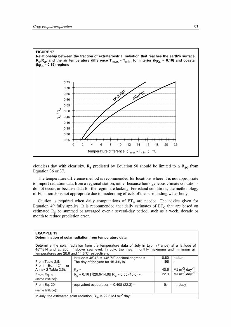
Crop evapotranspiration
61
cloudless day with clear sky. Rs predicted by Equation 50 should be limited to ≤ Rso from Equation 36 or 37.
The temperature difference method is recommended for locations where it is not appropriate to import radiation data from a regional station, either because homogeneous climate conditions do not occur, or because data for the region are lacking. For island conditions, the methodology of Equation 50 is not appropriate due to moderating effects of the surrounding water body.
Caution is required when daily computations of ETo are needed. The advice given for Equation 49 fully applies. It is recommended that daily estimates of ETo that are based on estimated Rs be summed or averaged over a several-day period, such as a week, decade or month to reduce prediction error.
EXAMPLE 15 Determination of solar radiation from temperature data Determine the solar radiation from the temperature data of July in Lyon (France) at a latitude of 45°43'N and at 200 m above sea level. In July, the mean monthly maximum and minimum air temperatures are 26.6 and 14.8°C respectively. From Table 2.5: From Eq. 21 or Annex 2 Table 2.6):
latitude = 45°43’ = +45.72° decimal degrees = The day of the year for 15 July is Ra =
0.80 196
40.6
radian - MJ m-2 day-1
From Eq. 50 (same latitude):
Rs = 0.16 [√(26.6-14.8)] Ra = 0.55 (40.6) = 22.3 MJ m-2 day-1
From Eq. 20
(same latitude): equivalent evaporation = 0.408 (22.3) = 9.1 mm/day
In July, the estimated solar radiation, Rs, is 22.3 MJ m-2 day-1
FIGURE 17 Relationship between the fraction of extraterrestrial radiation that reaches the earth's surface,Rs/Ra, and the air temperature difference Tmax - Tmin for interior (kRs = 0.16) and coastal (kRs = 0.19) regions
0 2 4 6 8 10 12 14 16 18 20 22
temperature difference (Tmax - Tmin ) °C
0.25
0.30
0.35
0.40
0.45
0.50
0.55
0.60
0.65
0.70
0.75
Rs /
Ra
interiorcoasta
l
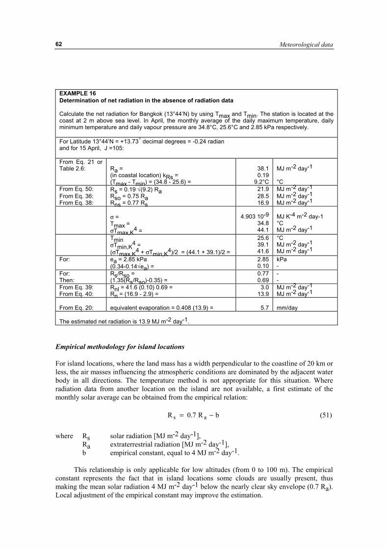
Meteorological data
62
EXAMPLE 16 Determination of net radiation in the absence of radiation data Calculate the net radiation for Bangkok (13°44’N) by using Tmax and Tmin. The station is located at the coast at 2 m above sea level. In April, the monthly average of the daily maximum temperature, daily minimum temperature and daily vapour pressure are 34.8°C, 25.6°C and 2.85 kPa respectively. For Latitude 13°44’N = +13.73° decimal degrees = -0.24 radian and for 15 April, J =105: From Eq. 21 or Table 2.6:
Ra = (in coastal location) kRs = (Tmax - Tmin) = (34.8 - 25.6) =
38.1 0.19
9.2°C
MJ m-2 day-1 °C
From Eq. 50: Rs = 0.19 √(9.2) Ra 21.9 MJ m-2 day-1 From Eq. 36: Rso = 0.75 Ra 28.5 MJ m-2 day-1 From Eq. 38: Rns = 0.77 Rs 16.9 MJ m-2 day-1
σ = Tmax = σTmax,K4 =
4.903 10-9
34.8 44.1
MJ K-4 m-2 day-1 °C MJ m-2 day-1
Tmin σTmin,K4 = (σTmax,K4 + σTmin,K4)/2 = (44.1 + 39.1)/2 =
25.6 39.1 41.6
°C MJ m-2 day-1 MJ m-2 day-1
For: ea = 2.85 kPa (0.34-0.14√ea) =
2.85 0.10
kPa -
For: Then:
Rs/Rso = (1.35(Rs/Rso)-0.35) =
0.77 0.69
- -
From Eq. 39: Rnl = 41.6 (0.10) 0.69 = 3.0 MJ m-2 day-1 From Eq. 40: Rn = (16.9 - 2.9) = 13.9 MJ m-2 day-1 From Eq. 20:
equivalent evaporation = 0.408 (13.9) =
5.7
mm/day
The estimated net radiation is 13.9 MJ m-2 day-1.
Empirical methodology for island locations For island locations, where the land mass has a width perpendicular to the coastline of 20 km or less, the air masses influencing the atmospheric conditions are dominated by the adjacent water body in all directions. The temperature method is not appropriate for this situation. Where radiation data from another location on the island are not available, a first estimate of the monthly solar average can be obtained from the empirical relation:
where Rs solar radiation [MJ m-2 day-1],
Ra extraterrestrial radiation [MJ m-2 day-1], b empirical constant, equal to 4 MJ m-2 day-1.
This relationship is only applicable for low altitudes (from 0 to 100 m). The empirical constant represents the fact that in island locations some clouds are usually present, thus making the mean solar radiation 4 MJ m-2 day-1 below the nearly clear sky envelope (0.7 Ra). Local adjustment of the empirical constant may improve the estimation.
bR7.0R as −= (51)
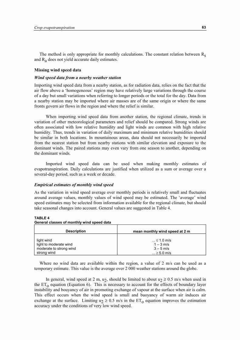
Crop evapotranspiration
63
The method is only appropriate for monthly calculations. The constant relation between Rs and Ra does not yield accurate daily estimates. Missing wind speed data
Wind speed data from a nearby weather station
Importing wind speed data from a nearby station, as for radiation data, relies on the fact that the air flow above a ‘homogeneous’ region may have relatively large variations through the course of a day but small variations when referring to longer periods or the total for the day. Data from a nearby station may be imported where air masses are of the same origin or where the same fronts govern air flows in the region and where the relief is similar. When importing wind speed data from another station, the regional climate, trends in variation of other meteorological parameters and relief should be compared. Strong winds are often associated with low relative humidity and light winds are common with high relative humidity. Thus, trends in variation of daily maximum and minimum relative humidities should be similar in both locations. In mountainous areas, data should not necessarily be imported from the nearest station but from nearby stations with similar elevation and exposure to the dominant winds. The paired stations may even vary from one season to another, depending on the dominant winds. Imported wind speed data can be used when making monthly estimates of evapotranspiration. Daily calculations are justified when utilized as a sum or average over a several-day period, such as a week or decade. Empirical estimates of monthly wind speed
As the variation in wind speed average over monthly periods is relatively small and fluctuates around average values, monthly values of wind speed may be estimated. The ‘average’ wind speed estimates may be selected from information available for the regional climate, but should take seasonal changes into account. General values are suggested in Table 4. TABLE 4 General classes of monthly wind speed data
Description
mean monthly wind speed at 2 m
light wind light to moderate wind moderate to strong wind strong wind
... ≤ 1.0 m/s
1 – 3 m/s 3 – 5 m/s
... ≥ 5.0 m/s Where no wind data are available within the region, a value of 2 m/s can be used as a temporary estimate. This value is the average over 2 000 weather stations around the globe. In general, wind speed at 2 m, u2, should be limited to about u2 ≥ 0.5 m/s when used in the ETo equation (Equation 6). This is necessary to account for the effects of boundary layer instability and bouyancy of air in promoting exchange of vapour at the surface when air is calm. This effect occurs when the wind speed is small and buoyancy of warm air induces air exchange at the surface. Limiting u2 ≥ 0.5 m/s in the ETo equation improves the estimation accuracy under the conditions of very low wind speed.
Meteorological data
64
Minimum data requirements This section has shown how solar radiation, vapour pressure and wind data can be estimated when missing. Many of the suggested procedures rely upon maximum and minimum air temperature measurements. Unfortunately, there is no dependable way to estimate air temperature when it is missing. Therefore it is suggested that maximum and minimum daily air temperature data are the minimum data requirements necessary to apply the FAO Penman-Monteith method. An alternative equation for ETo when weather data are missing When solar radiation data, relative humidity data and/or wind speed data are missing, they should be estimated using the procedures presented in this section. As an alternative, ETo can be estimated using the Hargreaves ETo equation where: a
5.0minmaxmeano R)TT()8.17T(0023.0ET −+= (52)
where all parameters have been previously defined. Units for both ETo and Ra in Equation 52 are mm day-1. Equation 52 should be verified in each new region by comparing with estimates by the FAO Penman-Monteith equation (Equation 6) at weather stations where solar radiation, air temperature, humidity, and wind speed are measured. If necessary, Equation 52 can be calibrated on a monthly or annual basis by determining empirical coefficients where ETo = a + b ETo Eq.52, where the “Eq. 52” subscript refers to ETo predicted using Equation 52. The coefficients a and b can be determined by regression analyses or by visual fitting. In general, estimating solar radiation, vapor pressure and wind speed as described in Equations 48 to 51 and Table 4 and then utilizing these estimates in Equation 6 (the FAO Penman-Monteith equation) will provide somewhat more accurate estimates as compared to estimating ETo directly using Equation 52. This is due to the ability of the estimation equations to incorporate general climatic characteristics such as high or low wind speed or high or low relative humidity into the ETo estimate made using Equation 6.
Equation 52 has a tendency to underpredict under high wind conditions (u2 > 3 m/s) and to overpredict under conditions of high relative humidity.
Crop evapotranspiration
65
Chapter 4
Determination of ETo This chapter demonstrates how the crop reference evapotranspiration (ETo) is determined either from meteorological data or from pan evaporation.
The FAO Penman-Monteith method is maintained as the sole standard method for the computation of ETo from meteorological data. The method itself is introduced in Chapter 2, and the computation of all data required for the calculation of ETo is discussed in Chapter 3. This chapter presents guidelines to calculate ETo with different time steps, ranging from hours to months, and with missing climatic data. The ETo calculation can be done by hand with the help of a calculation sheet, or by means of a computer.
ETo can also be estimated from the evaporation loss from a water surface. The procedure to obtain ETo from pan evaporation and the coefficients for different types of pans are presented in this chapter. PENMAN-MONTEITH EQUATION From the original Penman-Monteith equation and the equations of the aerodynamic and canopy resistance, the FAO Penman-Monteith equation has been derived in Chapter 2:
where ETo reference evapotranspiration [mm day-1],
Rn net radiation at the crop surface [MJ m-2 day-1], G soil heat flux density [MJ m-2 day-1], T air temperature at 2 m height [°C], u2 wind speed at 2 m height [m s-1], es saturation vapour pressure [kPa], ea actual vapour pressure [kPa], es-ea saturation vapour pressure deficit [kPa], ∆ slope vapour pressure curve [kPa °C-1], γ psychrometric constant [kPa °C-1].
The FAO Penman-Monteith equation determines the evapotranspiration from the
hypothetical grass reference surface and provides a standard to which evapotranspiration in
)u34.01(
)ee(u273T
900)GR(408.0
2
as2n
oET+γ+∆
−+
γ+−∆= (6)
Determination of ETo
66
different periods of the year or in other regions can be compared and to which the evapotranspiration from other crops can be related. Calculation procedure Calculation sheet ETo can be estimated by means of the calculation sheet presented in Box 11. The calculation sheet refers to tables in Annex II for the determination of some of the climatic parameters. The calculation procedure consists of the following steps: 1. Derivation of some climatic parameters from the daily maximum (Tmax) and minimum
(Tmin) air temperature, altitude (z) and mean wind speed (u2). 2. Calculation of the vapour pressure deficit (es-ea). The saturation vapour pressure (es) is
derived from Tmax and Tmin, while the actual vapour pressure (ea) can be derived from the dewpoint temperature (Tdew), from maximum (RHmax) and minimum (RHmin) relative humidity, from the maximum (RHmax), or from mean relative humidity (RHmean).
3. Determination of the net radiation (Rn) as the difference between the net shortwave radiation (Rns) and the net longwave radiation (Rnl). In the calculation sheet, the effect of soil heat flux (G) is ignored for daily calculations as the magnitude of the flux in this case is relatively small. The net radiation, expressed in MJ m-2 day-1, is converted to mm/day (equivalent evaporation) in the FAO Penman-Monteith equation by using 0.408 as the conversion factor within the equation.
4. ETo is obtained by combining the results of the previous steps.
Examples 17 and 20 present typical examples using the calculation sheet. Computerized calculations Calculations of the reference crop evapotranspiration ETo are often computerized. The calculation procedures of all data required for the calculation of ETo by means of the FAO Penman-Monteith equation are presented in Chapter 3. Typical sequences in which the calculations can be executed are given in the calculation sheets. The procedures presented in Boxes 7 (vapour pressure deficit), 9 (extraterrestrial radiation and daylight hours), 10 (net radiation) and 11 (ETo) can be used when developing a spreadsheet or computer program to calculate ETo.
Many software packages already use the FAO Penman-Monteith equation to assess the reference evapotranspiration. As an example, the output of CROPWAT, the FAO software for irrigation scheduling, is presented in Figure 18. ETo calculated with different time steps The selection of the time step with which ETo is calculated depends on the purpose of the calculation, the accuracy required and the time step of the climatic data available.
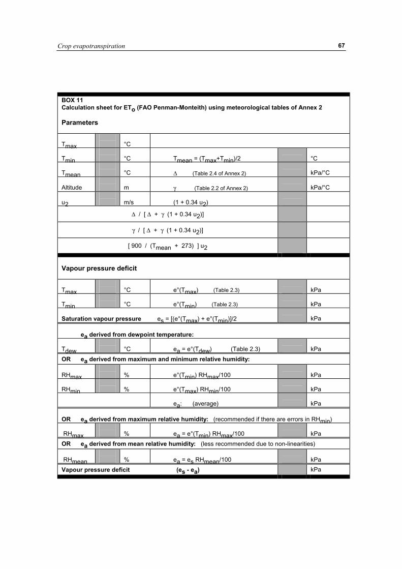
Crop evapotranspiration
67
BOX 11 Calculation sheet for ETo (FAO Penman-Monteith) using meteorological tables of Annex 2 Parameters Tmax
°C
Tmin
°C
Tmean = (Tmax+Tmin)/2
°C
Tmean
°C
∆ (Table 2.4 of Annex 2)
kPa/°C
Altitude
m
γ (Table 2.2 of Annex 2)
kPa/°C
u2
m/s
(1 + 0.34 u2)
∆ / [ ∆ + γ (1 + 0.34 u2)]
γ / [ ∆ + γ (1 + 0.34 u2)]
[ 900 / (Tmean + 273) ] u2
Vapour pressure deficit Tmax
°C
e°(Tmax) (Table 2.3)
kPa
Tmin
°C
e°(Tmin) (Table 2.3)
kPa
Saturation vapour pressure es = [(e°(Tmax) + e°(Tmin)]/2
kPa
ea derived from dewpoint temperature: Tdew
°C
ea = e°(Tdew) (Table 2.3)
kPa
OR ea derived from maximum and minimum relative humidity: RHmax
%
e°(Tmin) RHmax/100
kPa
RHmin
%
e°(Tmax) RHmin/100
kPa
ea: (average)
kPa
OR ea derived from maximum relative humidity: (recommended if there are errors in RHmin) RHmax
%
ea = e°(Tmin) RHmax/100
kPa
OR ea derived from mean relative humidity: (less recommended due to non-linearities) RHmean
%
ea = es RHmean/100
kPa
Vapour pressure deficit (es - ea) kPa
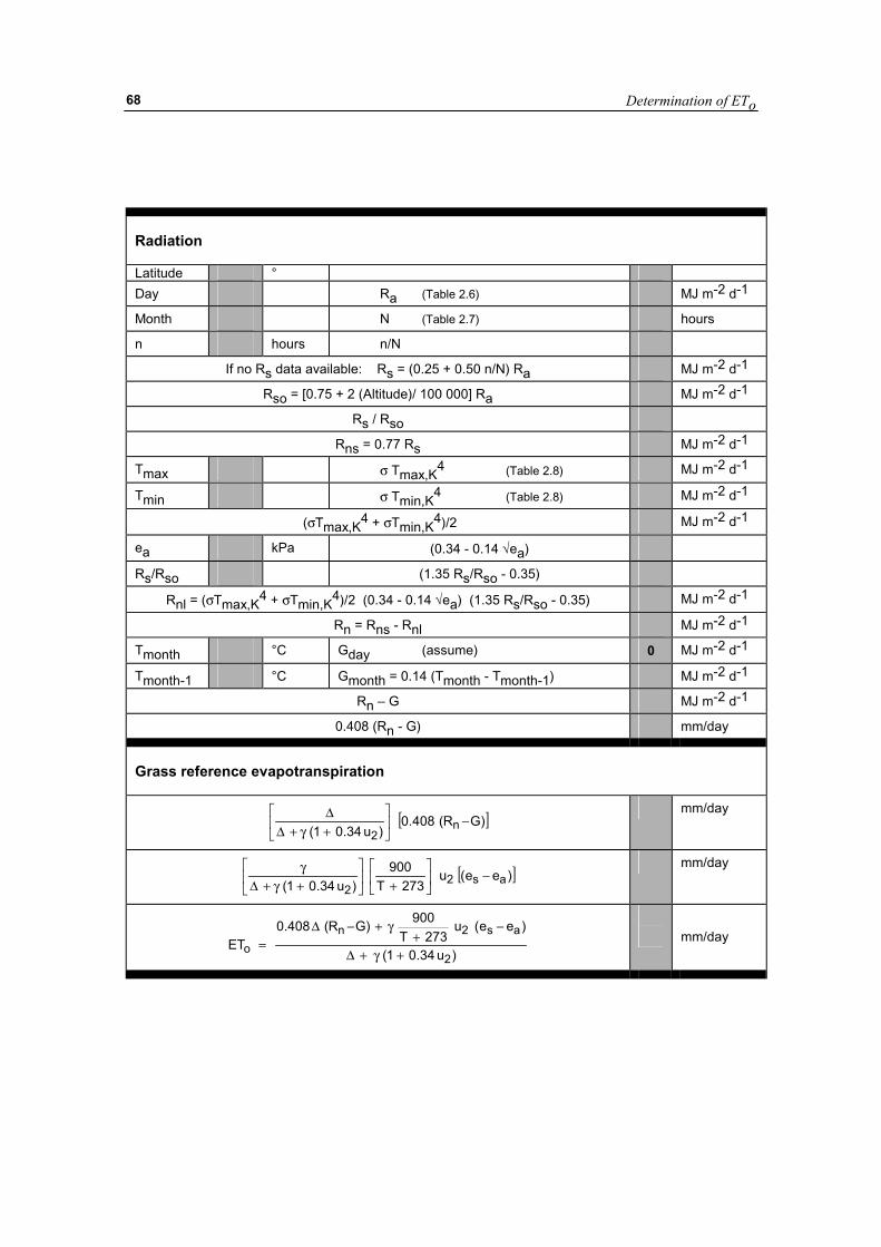
Determination of ETo
68
Radiation Latitude ° Day Ra (Table 2.6) MJ m-2 d-1
Month N (Table 2.7) hours
n hours n/N
If no Rs data available: Rs = (0.25 + 0.50 n/N) Ra MJ m-2 d-1
Rso = [0.75 + 2 (Altitude)/ 100 000] Ra MJ m-2 d-1
Rs / Rso
Rns = 0.77 Rs MJ m-2 d-1
Tmax σ Tmax,K4 (Table 2.8) MJ m-2 d-1
Tmin σ Tmin,K4 (Table 2.8) MJ m-2 d-1
(σTmax,K4 + σTmin,K4)/2 MJ m-2 d-1
ea kPa (0.34 - 0.14 √ea)
Rs/Rso (1.35 Rs/Rso - 0.35)
Rnl = (σTmax,K4 + σTmin,K4)/2 (0.34 - 0.14 √ea) (1.35 Rs/Rso - 0.35) MJ m-2 d-1
Rn = Rns - Rnl MJ m-2 d-1
Tmonth °C Gday (assume) 0 MJ m-2 d-1
Tmonth-1 °C Gmonth = 0.14 (Tmonth - Tmonth-1) MJ m-2 d-1
Rn – G MJ m-2 d-1
0.408 (Rn - G) mm/day
Grass reference evapotranspiration
[ ])GR(408.0)u34.01( n
2−�
�
���
�
+γ+∆∆
mm/day
[ ])ee(u273T
900)u34.01( as2
2−�
�
���
�
+��
���
�
+γ+∆γ
mm/day
)u34.01(
)ee(u273T
900)GR(408.0ET
2
as2no +γ+∆
−+
γ+−∆=
mm/day
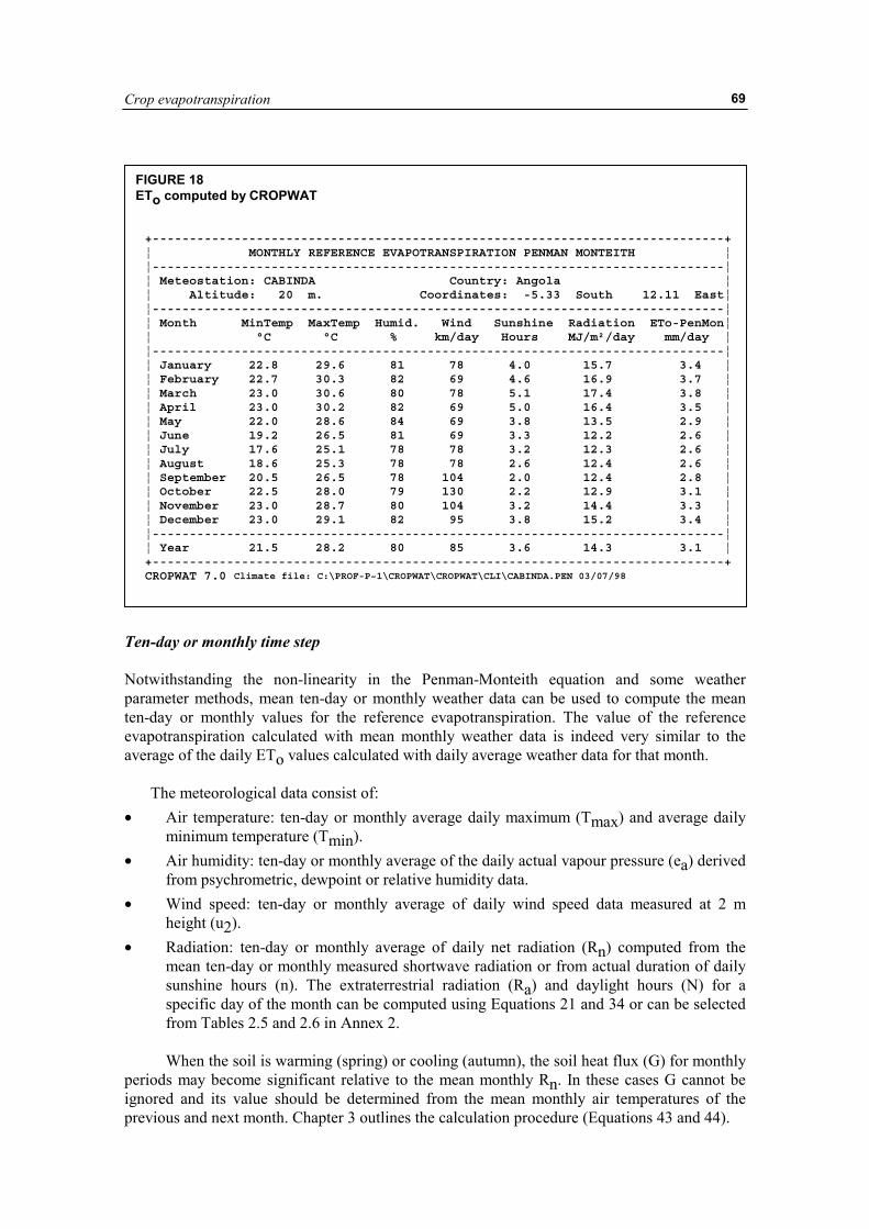
Crop evapotranspiration
69
Ten-day or monthly time step Notwithstanding the non-linearity in the Penman-Monteith equation and some weather parameter methods, mean ten-day or monthly weather data can be used to compute the mean ten-day or monthly values for the reference evapotranspiration. The value of the reference evapotranspiration calculated with mean monthly weather data is indeed very similar to the average of the daily ETo values calculated with daily average weather data for that month.
The meteorological data consist of: • Air temperature: ten-day or monthly average daily maximum (Tmax) and average daily
minimum temperature (Tmin). • Air humidity: ten-day or monthly average of the daily actual vapour pressure (ea) derived
from psychrometric, dewpoint or relative humidity data. • Wind speed: ten-day or monthly average of daily wind speed data measured at 2 m
height (u2). • Radiation: ten-day or monthly average of daily net radiation (Rn) computed from the
mean ten-day or monthly measured shortwave radiation or from actual duration of daily sunshine hours (n). The extraterrestrial radiation (Ra) and daylight hours (N) for a specific day of the month can be computed using Equations 21 and 34 or can be selected from Tables 2.5 and 2.6 in Annex 2.
When the soil is warming (spring) or cooling (autumn), the soil heat flux (G) for monthly
periods may become significant relative to the mean monthly Rn. In these cases G cannot be ignored and its value should be determined from the mean monthly air temperatures of the previous and next month. Chapter 3 outlines the calculation procedure (Equations 43 and 44).
FIGURE 18 ETo computed by CROPWAT
+-----------------------------------------------------------------------------+¦ MONTHLY REFERENCE EVAPOTRANSPIRATION PENMAN MONTEITH ¦¦-----------------------------------------------------------------------------¦¦ Meteostation: CABINDA Country: Angola ¦¦ Altitude: 20 m. Coordinates: -5.33 South 12.11 East¦¦-----------------------------------------------------------------------------¦¦ Month MinTemp MaxTemp Humid. Wind Sunshine Radiation ETo-PenMon¦¦ °C °C % km/day Hours MJ/m²/day mm/day ¦¦-----------------------------------------------------------------------------¦¦ January 22.8 29.6 81 78 4.0 15.7 3.4 ¦¦ February 22.7 30.3 82 69 4.6 16.9 3.7 ¦¦ March 23.0 30.6 80 78 5.1 17.4 3.8 ¦¦ April 23.0 30.2 82 69 5.0 16.4 3.5 ¦¦ May 22.0 28.6 84 69 3.8 13.5 2.9 ¦¦ June 19.2 26.5 81 69 3.3 12.2 2.6 ¦¦ July 17.6 25.1 78 78 3.2 12.3 2.6 ¦¦ August 18.6 25.3 78 78 2.6 12.4 2.6 ¦¦ September 20.5 26.5 78 104 2.0 12.4 2.8 ¦¦ October 22.5 28.0 79 130 2.2 12.9 3.1 ¦¦ November 23.0 28.7 80 104 3.2 14.4 3.3 ¦¦ December 23.0 29.1 82 95 3.8 15.2 3.4 ¦¦-----------------------------------------------------------------------------¦¦ Year 21.5 28.2 80 85 3.6 14.3 3.1 ¦+-----------------------------------------------------------------------------+CROPWAT 7.0 Climate file: C:\PROF-P~1\CROPWAT\CROPWAT\CLI\CABINDA.PEN 03/07/98
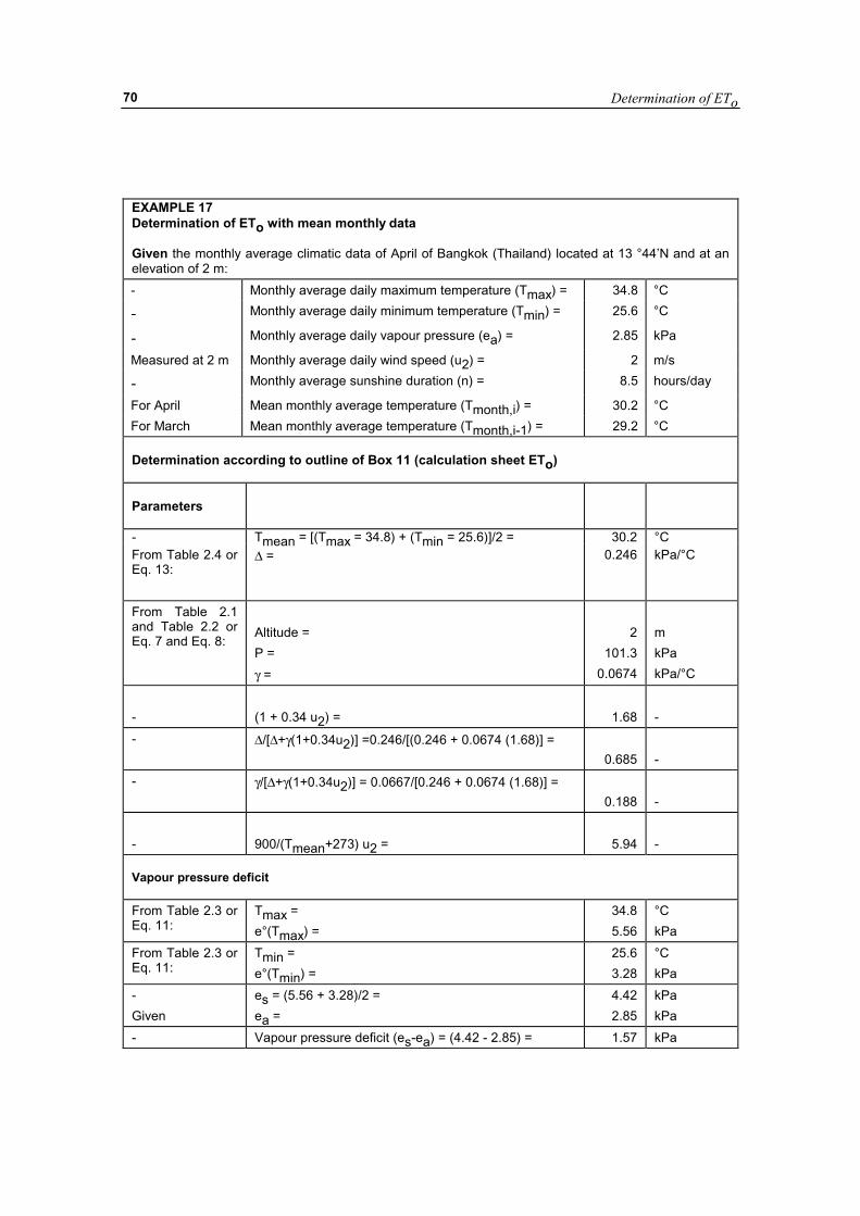
Determination of ETo
70
EXAMPLE 17 Determination of ETo with mean monthly data Given the monthly average climatic data of April of Bangkok (Thailand) located at 13 °44’N and at an elevation of 2 m: - Monthly average daily maximum temperature (Tmax) = 34.8 °C
- Monthly average daily minimum temperature (Tmin) = 25.6 °C
- Monthly average daily vapour pressure (ea) = 2.85 kPa Measured at 2 m Monthly average daily wind speed (u2) = 2 m/s - Monthly average sunshine duration (n) = 8.5 hours/day For April Mean monthly average temperature (Tmonth,i) = 30.2 °C For March Mean monthly average temperature (Tmonth,i-1) = 29.2 °C Determination according to outline of Box 11 (calculation sheet ETo) Parameters
- Tmean = [(Tmax = 34.8) + (Tmin = 25.6)]/2 = 30.2 °C From Table 2.4 or Eq. 13:
∆ = 0.246 kPa/°C
From Table 2.1 and Table 2.2 or Eq. 7 and Eq. 8:
Altitude = P = γ =
2
101.3 0.0674
m kPa kPa/°C
-
(1 + 0.34 u2) =
1.68
-
-
∆/[∆+γ(1+0.34u2)] =0.246/[(0.246 + 0.0674 (1.68)] = 0.685
-
-
γ/[∆+γ(1+0.34u2)] = 0.0667/[0.246 + 0.0674 (1.68)] = 0.188
-
-
900/(Tmean+273) u2 =
5.94
-
Vapour pressure deficit From Table 2.3 or Eq. 11:
Tmax = e°(Tmax) =
34.8 5.56
°C kPa
From Table 2.3 or Eq. 11:
Tmin = e°(Tmin) =
25.6 3.28
°C kPa
- Given
es = (5.56 + 3.28)/2 = ea =
4.42 2.85
kPa kPa
- Vapour pressure deficit (es-ea) = (4.42 - 2.85) = 1.57 kPa
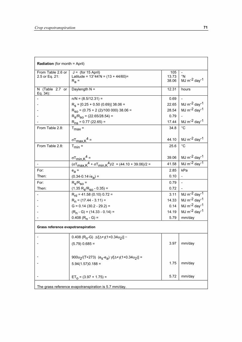
Crop evapotranspiration
71
Radiation (for month = April) From Table 2.6 or 2.5 or Eq. 21:
J = (for 15 April) Latitude = 13°44’N = (13 + 44/60)= Ra =
105 13.73 38.06
- °N MJ m-2 day-1
N (Table 2.7 or Eq. 34):
Daylength N =
12.31 hours
- n/N = (8.5/12.31) = 0.69 - - Rs = [0.25 + 0.50 (0.69)] 38.06 = 22.65 MJ m-2 day-1 - Rso = (0.75 + 2 (2)/100 000) 38.06 = 28.54 MJ m-2 day-1 - Rs/Rso = (22.65/28.54) = 0.79 - - Rns = 0.77 (22.65) = 17.44 MJ m-2 day-1 From Table 2.8: Tmax =
σTmax,K4 =
34.8
44.10
°C MJ m-2 day-1
From Table 2.8: Tmin = σTmin,K4 =
25.6
39.06
°C MJ m-2 day-1
- (σTmax,K4 + σTmin,K4)/2 = (44.10 + 39.06)/2 = 41.58 MJ m-2 day-1
For: Then:
ea = (0.34-0.14√ea) =
2.85 0.10
kPa -
For: Then:
Rs/Rso = (1.35 Rs/Rso - 0.35) =
0.79 0.72
- -
- - - - -
Rnl = 41.58 (0.10) 0.72 = Rn = (17.44 - 3.11) = G = 0.14 (30.2 - 29.2) = (Rn - G) = (14.33 - 0.14) = 0.408 (Rn - G) =
3.11 14.33
0.14 14.19
5.79
MJ m-2 day-1 MJ m-2 day-1 MJ m-2 day-1 MJ m-2 day-1 mm/day
Grass reference evapotranspiration -
-
-
-
-
0.408 (Rn-G) ∆/[∆+γ(1+0.34u2)] =
(5.79) 0.685 =
900u2/(T+273) (es-ea) γ/[∆+γ(1+0.34u2)] =
5.94(1.57)0.188 =
ETo = (3.97 + 1.75) =
3.97
1.75
5.72
mm/day
mm/day
mm/day
The grass reference evapotranspiration is 5.7 mm/day.
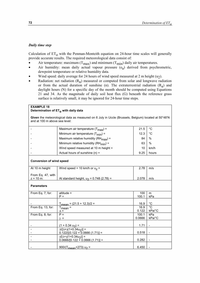
Determination of ETo
72
Daily time step Calculation of ETo with the Penman-Monteith equation on 24-hour time scales will generally provide accurate results. The required meteorological data consist of: • Air temperature: maximum (Tmax) and minimum (Tmin) daily air temperatures. • Air humidity: mean daily actual vapour pressure (ea) derived from psychrometric,
dewpoint temperature or relative humidity data. • Wind speed: daily average for 24 hours of wind speed measured at 2 m height (u2). • Radiation: net radiation (Rn) measured or computed from solar and longwave radiation
or from the actual duration of sunshine (n). The extraterrestrial radiation (Ra) and daylight hours (N) for a specific day of the month should be computed using Equations 21 and 34. As the magnitude of daily soil heat flux (G) beneath the reference grass surface is relatively small, it may be ignored for 24-hour time steps.
EXAMPLE 18 Determination of ETo with daily data Given the meteorological data as measured on 6 July in Uccle (Brussels, Belgium) located at 50°48’N and at 100 m above sea level: - - - - - -
Maximum air temperature (Tmax) = Minimum air temperature (Tmin) = Maximum relative humidity (RHmax) = Minimum relative humidity (RHmin) = Wind speed measured at 10 m height = Actual hours of sunshine (n) =
21.5 12.3
84 63 10
9.25
°C °C % % km/h hours
Conversion of wind speed At 10 m height From Eq. 47, with z = 10 m:
Wind speed = 10 km/h or uz = At standard height, u2 = 0.748 (2.78) =
2.78
2.078
m/s m/s
Parameters From Eq. 7, for:
altitude = P =
100 100.1
m kPa
-
Tmean = (21.5 + 12.3)/2 =
16.9
°C
From Eq. 13, for:
Tmean = ∆ =
16.9 0.122
°C kPa/°C
From Eq. 8, for:
P = γ =
100.1 0.0666
kPa kPa/°C
-
(1 + 0.34 u2) =
1.71
-
- -
∆/[∆+γ(1+0.34u2)] = 0.122/[(0.122 + 0.0666 (1.71)] =
0.518
-
- -
γ/[∆+γ(1+0.34u2)] = 0.0666/[0.122 + 0.0666 (1.71)] =
0.282
-
-
900/(Tmean+273) u2 =
6.450
-
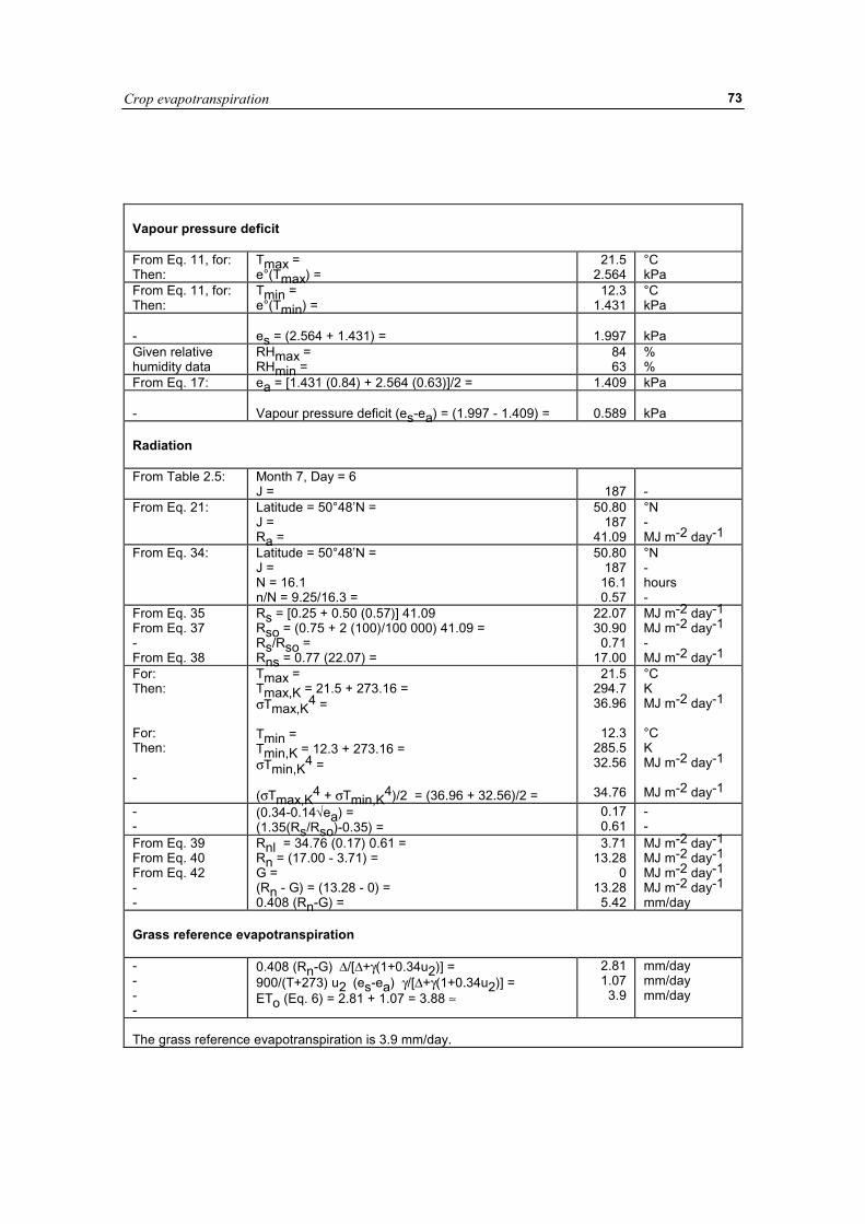
Crop evapotranspiration
73
Vapour pressure deficit From Eq. 11, for: Then:
Tmax = e°(Tmax) =
21.5 2.564
°C kPa
From Eq. 11, for: Then:
Tmin = e°(Tmin) =
12.3 1.431
°C kPa
-
es = (2.564 + 1.431) =
1.997
kPa
Given relative humidity data
RHmax = RHmin =
84 63
% %
From Eq. 17: ea = [1.431 (0.84) + 2.564 (0.63)]/2 = 1.409 kPa -
Vapour pressure deficit (es-ea) = (1.997 - 1.409) =
0.589
kPa
Radiation From Table 2.5: Month 7, Day = 6
J =
187 -
From Eq. 21: Latitude = 50°48’N = J = Ra =
50.80 187
41.09
°N - MJ m-2 day-1
From Eq. 34:
Latitude = 50°48’N = J = N = 16.1 n/N = 9.25/16.3 =
50.80 187
16.1 0.57
°N - hours -
From Eq. 35 From Eq. 37 - From Eq. 38
Rs = [0.25 + 0.50 (0.57)] 41.09 Rso = (0.75 + 2 (100)/100 000) 41.09 = Rs/Rso = Rns = 0.77 (22.07) =
22.07 30.90
0.71 17.00
MJ m-2 day-1 MJ m-2 day-1 - MJ m-2 day-1
For: Then: For: Then: -
Tmax = Tmax,K = 21.5 + 273.16 = σTmax,K4 = Tmin = Tmin,K = 12.3 + 273.16 = σTmin,K4 = (σTmax,K4 + σTmin,K4)/2 = (36.96 + 32.56)/2 =
21.5 294.7 36.96
12.3
285.5 32.56
34.76
°C K MJ m-2 day-1 °C K MJ m-2 day-1 MJ m-2 day-1
- -
(0.34-0.14√ea) = (1.35(Rs/Rso)-0.35) =
0.17 0.61
- -
From Eq. 39 From Eq. 40 From Eq. 42 - -
Rnl = 34.76 (0.17) 0.61 = Rn = (17.00 - 3.71) = G = (Rn - G) = (13.28 - 0) = 0.408 (Rn-G) =
3.71 13.28
0 13.28
5.42
MJ m-2 day-1 MJ m-2 day-1 MJ m-2 day-1 MJ m-2 day-1 mm/day
Grass reference evapotranspiration - - - -
0.408 (Rn-G) ∆/[∆+γ(1+0.34u2)] = 900/(T+273) u2 (es-ea) γ/[∆+γ(1+0.34u2)] = ETo (Eq. 6) = 2.81 + 1.07 = 3.88 ≈
2.81 1.07
3.9
mm/day mm/day mm/day
The grass reference evapotranspiration is 3.9 mm/day.
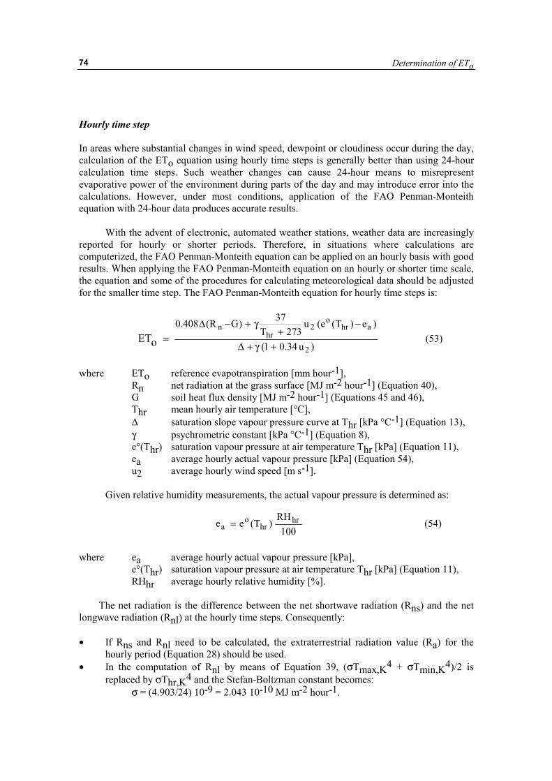
Determination of ETo
74
Hourly time step In areas where substantial changes in wind speed, dewpoint or cloudiness occur during the day, calculation of the ETo equation using hourly time steps is generally better than using 24-hour calculation time steps. Such weather changes can cause 24-hour means to misrepresent evaporative power of the environment during parts of the day and may introduce error into the calculations. However, under most conditions, application of the FAO Penman-Monteith equation with 24-hour data produces accurate results.
With the advent of electronic, automated weather stations, weather data are increasingly reported for hourly or shorter periods. Therefore, in situations where calculations are computerized, the FAO Penman-Monteith equation can be applied on an hourly basis with good results. When applying the FAO Penman-Monteith equation on an hourly or shorter time scale, the equation and some of the procedures for calculating meteorological data should be adjusted for the smaller time step. The FAO Penman-Monteith equation for hourly time steps is:
)u34.01(
)e)T(e(u273T
37)GR(408.0
2
ahro
2hr
n
oET+γ+∆
−+
γ+−∆= (53)
where ETo reference evapotranspiration [mm hour-1],
Rn net radiation at the grass surface [MJ m-2 hour-1] (Equation 40), G soil heat flux density [MJ m-2 hour-1] (Equations 45 and 46), Thr mean hourly air temperature [°C], ∆ saturation slope vapour pressure curve at Thr [kPa °C-1] (Equation 13), γ psychrometric constant [kPa °C-1] (Equation 8), e°(Thr) saturation vapour pressure at air temperature Thr [kPa] (Equation 11), ea average hourly actual vapour pressure [kPa] (Equation 54), u2 average hourly wind speed [m s-1].
Given relative humidity measurements, the actual vapour pressure is determined as:
where ea average hourly actual vapour pressure [kPa], e°(Thr) saturation vapour pressure at air temperature Thr [kPa] (Equation 11), RHhr average hourly relative humidity [%].
The net radiation is the difference between the net shortwave radiation (Rns) and the net longwave radiation (Rnl) at the hourly time steps. Consequently:
• If Rns and Rnl need to be calculated, the extraterrestrial radiation value (Ra) for the
hourly period (Equation 28) should be used. • In the computation of Rnl by means of Equation 39, (σTmax,K4 + σTmin,K4)/2 is
replaced by σThr,K4 and the Stefan-Boltzman constant becomes: σ = (4.903/24) 10-9 = 2.043 10-10 MJ m-2 hour-1.
100
RH)T(ee hr
hro
a = (54)
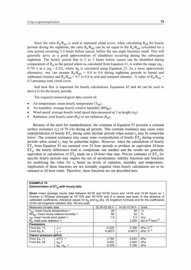
Crop evapotranspiration
75
Since the ratio Rs/Rso is used to represent cloud cover, when calculating Rnl for hourly periods during the nighttime, the ratio Rs/Rso can be set equal to the Rs/Rso calculated for a time period occurring 2-3 hours before sunset, before the sun angle becomes small. This will generally serve as a good approximation of cloudiness occurring during the subsequent nighttime. The hourly period that is 2 to 3 hours before sunset can be identified during computation of Ra as the period where ω, calculated from Equation 31, is within the range (ωs - 0.79) ≤ ω ≤ (ωs - 0.52), where ωs is calculated using Equation 25. As a more approximate alternative, one can assume Rs/Rso = 0.4 to 0.6 during nighttime periods in humid and subhumid climates and Rs/Rso = 0.7 to 0.8 in arid and semiarid climates. A value of Rs/Rso = 0.3 presumes total cloud cover.
Soil heat flux is important for hourly calculations. Equations 45 and 46 can be used to derive G for the hourly periods.
The required meteorological data consist of:
• Air temperature: mean hourly temperature (Thr). • Air humidity: average hourly relative humidity (RHhr). • Wind speed: average hourly wind speed data measured at 2 m height (u2). • Radiation: total hourly solar (Rs) or net radiation (Rn).
Because of the need for standardization, the constants in Equation 53 presume a constant surface resistance (rs) of 70 s/m during all periods. This constant resistance may cause some underprediction of hourly ETo during some daytime periods when actual rs may be somewhat lower. The constant resistance may cause some overprediction of hourly ETo during evening periods when actual rs may be somewhat higher. However, when the calculations of hourly ETo from Equation 53 are summed over 24 hour periods to produce an equivalent 24-hour ETo, the hourly differences tend to compensate one another and the results are generally equivalent to calculations of ETo made on a 24-hour time step. Precise estimates of ETo for specific hourly periods may require the use of aerodynamic stability functions and functions for modifying the value for rs based on levels of radiation, humidity and temperature. Application of these functions are not normally required when hourly calculations are to be summed to 24-hour totals. Therefore, these functions are not described here.
EXAMPLE 19 Determination of ETo with hourly data Given mean average hourly data between 02.00 and 03.00 hours and 14.00 and 15.00 hours on 1 October in N’Diaye (Senegal) at 16°13'N and 16°15'W and 8 m above sea level. In the absence of calibrated coefficients, indicative values for as and bs (Eq. 35 Angstrom formula) and for the coefficients of the net longwave radiation (Eq. 39) are used. Measured climatic data 02.00-03.00 h 14.00-15.00 h Units Thr: mean hourly temperature = RHhr: mean hourly relative humidity = u2: mean hourly wind speed = Rs: total solar radiation =
28 90
1.9 -
38 52
3.3 2.450
°C % m/s MJ m-2 hour-1
Parameters From Eq. 13 From Eq. 8
∆ = γ =
0.220 0.0673
0.358 0.0673
kPa °C-1 kPa °C-1
Vapour pressure deficit From Eq. 11 From Eq. 54 -
eº(T) = ea = es - ea =
3.780 3.402 0.378
6.625 3.445 3.180
kPa kPa kPa
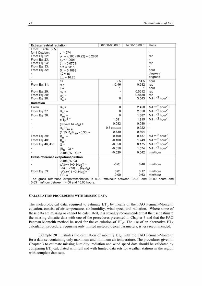
Determination of ETo
76
Extraterrestrial radiation 02.00-03.00 h 14.00-15.00 h Units From Table 2.5 for 1 October: From Eq. 22: From Eq. 23: From Eq. 24: From Eq. 33: From Eq. 32: - -
J = 274 ϕ = π/180 (16.22) = 0.2830 dr = 1.0001 δ = - 0.0753 b = 3.3315 Sc = 0.1889 Lz = 15 Lm = 16.25
- rad - rad - hour degrees degrees
- From Eq. 31: - From Eq. 29: From Eq. 30: From Eq. 28:
t = ω = tl = ω1 = ω2 = Ra =
2.5 -2.46
1 - - 0
14.5 0.682
1 0.5512 0.8130
3.543
hour rad hour rad rad MJ m-2 hour-1
Radiation Given From Eq. 37: From Eq. 38: - - - - From Eq. 39: From Eq. 40: From Eq. 46, 45: - -
Rs = Rso = Rns = σ TK4 = (0.34-0.14 √ea) = Rs/Rso = (1.35 Rs/Rso - 0.35) = Rnl = Rn = G = (Rn - G) = 0.408(Rn - G) =
0 0 0
1.681 0.082
0.8 (assumed) 0.730 0.100
-0.100 -0.050 -0.050 -0.020
2.450 2.658 1.887 1.915 0.080 0.922 0.894 0.137 1.749 0.175 1.574 0.642
MJ m-2 hour-1 MJ m-2 hour-1 MJ m-2 hour-1 MJ m-2 hour-1 - - - MJ m-2 hour-1 MJ m-2 hour-1 MJ m-2 hour-1 MJ m-2 hour-1 mm/hour
Grass reference evapotranspiration - - From Eq. 53:
0.408(Rn-G) ∆/[∆+γ(1+0.34u2)] = 37/(T+273) u2 (es-ea) γ/[∆+γ( 1 +0.34u2)= ETo =
-0.01
0.01 0.00
0.46
0.17 0.63
mm/hour mm/hour mm/hour
The grass reference evapotranspiration is 0.00 mm/hour between 02.00 and 03.00 hours and 0.63 mm/hour between 14.00 and 15.00 hours.
CALCULATION PROCEDURES WITH MISSING DATA The meteorological data, required to estimate ETo by means of the FAO Penman-Monteith equation, consist of air temperature, air humidity, wind speed and radiation. Where some of these data are missing or cannot be calculated, it is strongly recommended that the user estimate the missing climatic data with one of the procedures presented in Chapter 3 and that the FAO Penman-Monteith method be used for the calculation of ETo. The use of an alternative ETo calculation procedure, requiring only limited meteorological parameters, is less recommended.
Example 20 illustrates the estimation of monthly ETo with the FAO Penman-Monteith for a data set containing only maximum and minimum air temperature. The procedures given in Chapter 3 to estimate missing humidity, radiation and wind speed data should be validated by comparing ETo calculated with full and with limited data sets for weather stations in the region with complete data sets.
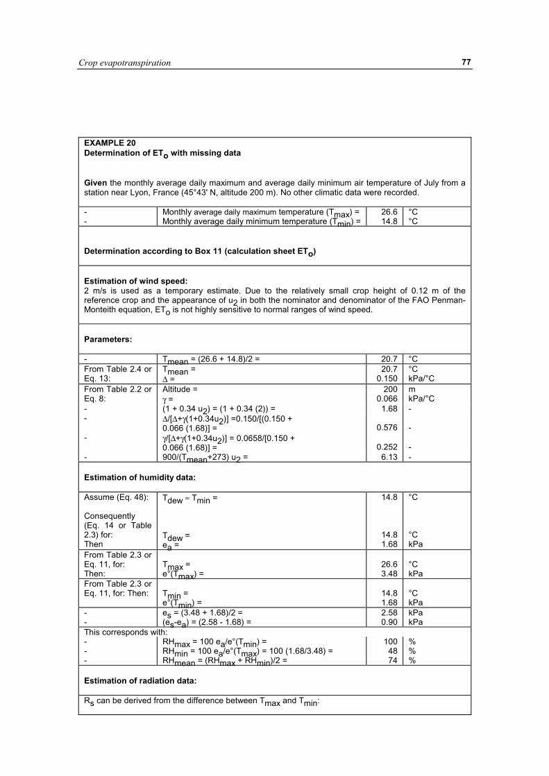
Crop evapotranspiration
77
EXAMPLE 20 Determination of ETo with missing data Given the monthly average daily maximum and average daily minimum air temperature of July from a station near Lyon, France (45°43' N, altitude 200 m). No other climatic data were recorded. - -
Monthly average daily maximum temperature (Tmax) = Monthly average daily minimum temperature (Tmin) =
26.6 14.8
°C °C
Determination according to Box 11 (calculation sheet ETo) Estimation of wind speed: 2 m/s is used as a temporary estimate. Due to the relatively small crop height of 0.12 m of the reference crop and the appearance of u2 in both the nominator and denominator of the FAO Penman-Monteith equation, ETo is not highly sensitive to normal ranges of wind speed. Parameters: - Tmean = (26.6 + 14.8)/2 = 20.7 °C From Table 2.4 or Eq. 13:
Tmean = ∆ =
20.7 0.150
°C kPa/°C
From Table 2.2 or Eq. 8:
Altitude = γ =
200 0.066
m kPa/°C
- (1 + 0.34 u2) = (1 + 0.34 (2)) = 1.68 - - ∆/[∆+γ(1+0.34u2)] =0.150/[(0.150 +
0.066 (1.68)] =
0.576 -
- γ/[∆+γ(1+0.34u2)] = 0.0658/[0.150 + 0.066 (1.68)] =
0.252
-
- 900/(Tmean+273) u2 = 6.13 - Estimation of humidity data: Assume (Eq. 48): Consequently (Eq. 14 or Table 2.3) for: Then
Tdew ≈ Tmin = Tdew = ea =
14.8
14.8 1.68
°C °C kPa
From Table 2.3 or Eq. 11, for: Then:
Tmax = e°(Tmax) =
26.6 3.48
°C kPa
From Table 2.3 or Eq. 11, for: Then:
Tmin = e°(Tmin) =
14.8 1.68
°C kPa
- -
es = (3.48 + 1.68)/2 = (es-ea) = (2.58 - 1.68) =
2.58 0.90
kPa kPa
This corresponds with: - - -
RHmax = 100 ea/e°(Tmin) = RHmin = 100 ea/e°(Tmax) = 100 (1.68/3.48) = RHmean = (RHmax + RHmin)/2 =
100 48 74
% % %
Estimation of radiation data: Rs can be derived from the difference between Tmax and Tmin:
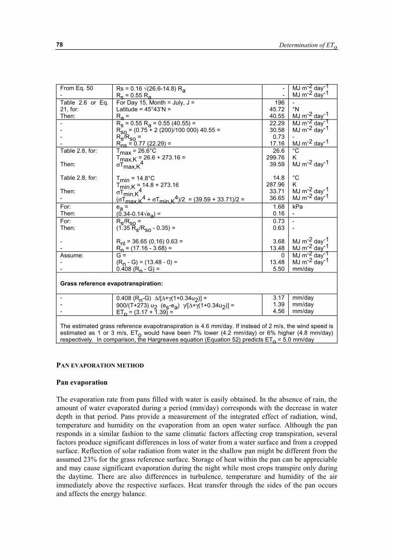
Determination of ETo
78
From Eq. 50 -
Rs = 0.16 √(26.6-14.8) Ra Rs = 0.55 Ra
- -
MJ m-2 day-1 MJ m-2 day-1
Table 2.6 or Eq. 21, for: Then:
For Day 15, Month = July, J = Latitude = 45°43’N = Ra =
196 45.72 40.55
- °N MJ m-2 day-1
- - - -
Rs = 0.55 Ra = 0.55 (40.55) = Rso = (0.75 + 2 (200)/100 000) 40.55 = Rs/Rso = Rns = 0.77 (22.29) =
22.29 30.58
0.73 17.16
MJ m-2 day-1 MJ m-2 day-1 - MJ m-2 day-1
Table 2.8, for: Then: Table 2.8, for: Then: -
Tmax = 26.6°C Tmax,K = 26.6 + 273.16 = σTmax,K4 Tmin = 14.8°C Tmin,K = 14.8 + 273.16 σTmin,K4 (σTmax,K4 + σTmin,K4)/2 = (39.59 + 33.71)/2 =
26.6 299.76
39.59
14.8 287.96
33.71 36.65
°C K MJ m-2 day-1 °C K MJ m-2 day-1 MJ m-2 day-1
For: Then:
ea = (0.34-0.14√ea) =
1.68 0.16
kPa -
For: Then: - -
Rs/Rso = (1.35 Rs/Rso - 0.35) = Rnl = 36.65 (0.16) 0.63 = Rn = (17.16 - 3.68) =
0.73 0.63
3.68
13.48
- - MJ m-2 day-1 MJ m-2 day-1
Assume: - -
G = (Rn - G) = (13.48 - 0) = 0.408 (Rn - G) =
0 13.48
5.50
MJ m-2 day-1 MJ m-2 day-1 mm/day
Grass reference evapotranspiration: - - -
0.408 (Rn-G) ∆/[∆+γ(1+0.34u2)] = 900/(T+273) u2 (es-ea) γ/[∆+γ(1+0.34u2)] = ETo = (3.17 + 1.39) =
3.17 1.39 4.56
mm/day mm/day mm/day
The estimated grass reference evapotranspiration is 4.6 mm/day. If instead of 2 m/s, the wind speed is estimated as 1 or 3 m/s, ETo would have been 7% lower (4.2 mm/day) or 6% higher (4.8 mm/day) respectively. In comparison, the Hargreaves equation (Equation 52) predicts ETo = 5.0 mm/day
PAN EVAPORATION METHOD Pan evaporation The evaporation rate from pans filled with water is easily obtained. In the absence of rain, the amount of water evaporated during a period (mm/day) corresponds with the decrease in water depth in that period. Pans provide a measurement of the integrated effect of radiation, wind, temperature and humidity on the evaporation from an open water surface. Although the pan responds in a similar fashion to the same climatic factors affecting crop transpiration, several factors produce significant differences in loss of water from a water surface and from a cropped surface. Reflection of solar radiation from water in the shallow pan might be different from the assumed 23% for the grass reference surface. Storage of heat within the pan can be appreciable and may cause significant evaporation during the night while most crops transpire only during the daytime. There are also differences in turbulence, temperature and humidity of the air immediately above the respective surfaces. Heat transfer through the sides of the pan occurs and affects the energy balance.
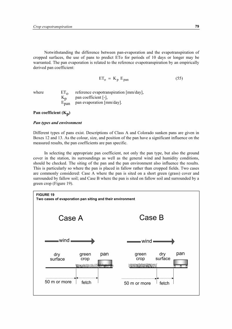
Crop evapotranspiration
79
Notwithstanding the difference between pan-evaporation and the evapotranspiration of cropped surfaces, the use of pans to predict ETo for periods of 10 days or longer may be warranted. The pan evaporation is related to the reference evapotranspiration by an empirically derived pan coefficient:
where ETo reference evapotranspiration [mm/day],
Kp pan coefficient [-], Epan pan evaporation [mm/day].
Pan coefficient (Kp) Pan types and environment Different types of pans exist. Descriptions of Class A and Colorado sunken pans are given in Boxes 12 and 13. As the colour, size, and position of the pan have a significant influence on the measured results, the pan coefficients are pan specific.
In selecting the appropriate pan coefficient, not only the pan type, but also the ground cover in the station, its surroundings as well as the general wind and humidity conditions, should be checked. The siting of the pan and the pan environment also influence the results. This is particularly so where the pan is placed in fallow rather than cropped fields. Two cases are commonly considered: Case A where the pan is sited on a short green (grass) cover and surrounded by fallow soil; and Case B where the pan is sited on fallow soil and surrounded by a green crop (Figure 19).
panpo EKET = (55)
FIGURE 19 Two cases of evaporation pan siting and their environment
wind wind
Case A Case B
drysurface
drysurface
green crop
green crop
pan pan
fetch fetch50 m or more 50 m or more
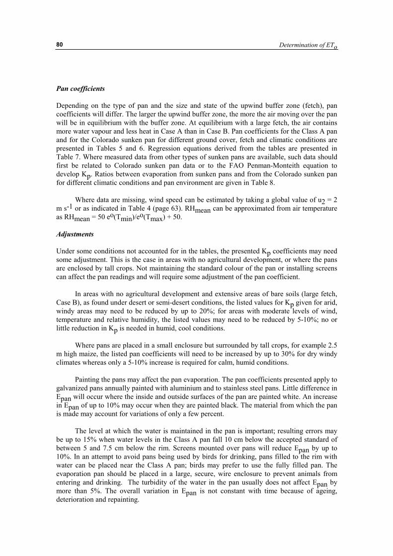
Determination of ETo
80
Pan coefficients Depending on the type of pan and the size and state of the upwind buffer zone (fetch), pan coefficients will differ. The larger the upwind buffer zone, the more the air moving over the pan will be in equilibrium with the buffer zone. At equilibrium with a large fetch, the air contains more water vapour and less heat in Case A than in Case B. Pan coefficients for the Class A pan and for the Colorado sunken pan for different ground cover, fetch and climatic conditions are presented in Tables 5 and 6. Regression equations derived from the tables are presented in Table 7. Where measured data from other types of sunken pans are available, such data should first be related to Colorado sunken pan data or to the FAO Penman-Monteith equation to develop Kp. Ratios between evaporation from sunken pans and from the Colorado sunken pan for different climatic conditions and pan environment are given in Table 8.
Where data are missing, wind speed can be estimated by taking a global value of u2 = 2 m s-1 or as indicated in Table 4 (page 63). RHmean can be approximated from air temperature as RHmean = 50 eo(Tmin)/eo(Tmax) + 50. Adjustments Under some conditions not accounted for in the tables, the presented Kp coefficients may need some adjustment. This is the case in areas with no agricultural development, or where the pans are enclosed by tall crops. Not maintaining the standard colour of the pan or installing screens can affect the pan readings and will require some adjustment of the pan coefficient.
In areas with no agricultural development and extensive areas of bare soils (large fetch, Case B), as found under desert or semi-desert conditions, the listed values for Kp given for arid, windy areas may need to be reduced by up to 20%; for areas with moderate levels of wind, temperature and relative humidity, the listed values may need to be reduced by 5-10%; no or little reduction in Kp is needed in humid, cool conditions.
Where pans are placed in a small enclosure but surrounded by tall crops, for example 2.5 m high maize, the listed pan coefficients will need to be increased by up to 30% for dry windy climates whereas only a 5-10% increase is required for calm, humid conditions.
Painting the pans may affect the pan evaporation. The pan coefficients presented apply to galvanized pans annually painted with aluminium and to stainless steel pans. Little difference in Epan will occur where the inside and outside surfaces of the pan are painted white. An increase in Epan of up to 10% may occur when they are painted black. The material from which the pan is made may account for variations of only a few percent.
The level at which the water is maintained in the pan is important; resulting errors may be up to 15% when water levels in the Class A pan fall 10 cm below the accepted standard of between 5 and 7.5 cm below the rim. Screens mounted over pans will reduce Epan by up to 10%. In an attempt to avoid pans being used by birds for drinking, pans filled to the rim with water can be placed near the Class A pan; birds may prefer to use the fully filled pan. The evaporation pan should be placed in a large, secure, wire enclosure to prevent animals from entering and drinking. The turbidity of the water in the pan usually does not affect Epan by more than 5%. The overall variation in Epan is not constant with time because of ageing, deterioration and repainting.
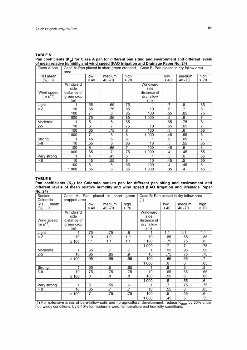
Crop evapotranspiration
81
TABLE 5 Pan coefficients (Kp) for Class A pan for different pan siting and environment and different levels of mean relative humidity and wind speed (FAO Irrigation and Drainage Paper No. 24)
Class A pan Case A: Pan placed in short green cropped area
Case B: Pan placed in dry fallow area
RH mean (%) �
low < 40
medium 40 -70
high > 70
low < 40
medium 40 -70
high > 70
Wind speed (m s-1)
Windward side
distance of green crop
(m)
Windward side
distance of dry fallow
(m)
Light 1 .55 .65 .75 1 .7 .8 .85 < 2 10 .65 .75 .85 10 .6 .7 .8 100 .7 .8 .85 100 .55 .65 .75 1 000 .75 .85 .85 1 000 .5 .6 .7 Moderate 1 .5 .6 .65 1 .65 .75 .8 2-5 10 .6 .7 .75 10 .55 .65 .7 100 .65 .75 .8 100 .5 .6 .65 1 000 .7 .8 .8 1 000 .45 .55 .6 Strong 1 .45 .5 .6 1 .6 .65 .7 5-8 10 .55 .6 .65 10 .5 .55 .65 100 .6 .65 .7 100 .45 .5 .6 1 000 .65 .7 .75 1 000 .4 .45 .55 Very strong 1 .4 .45 .5 1 .5 .6 .65 > 8 10 .45 .55 .6 10 .45 .5 .55 100 .5 .6 .65 100 .4 .45 .5 1 000 .55 .6 .65 1 000 .35 .4 .45
TABLE 6 Pan coefficients (Kp) for Colorado sunken pan for different pan siting and environment and different levels of mean relative humidity and wind speed (FAO Irrigation and Drainage Paper No. 24)
Sunken Colorado
Case A: Pan placed in short green cropped area
Case B: Pan placed in dry fallow area (1)
RH mean (%) �
low < 40
medium 40 -70
high > 70
low < 40
medium 40 -70
high > 70
Wind speed (m s-1)
Windward side
distance of green crop
(m)
Windward side
distance of dry fallow
(m)
Light 1 .75 .75 .8 1 1.1 1.1 1.1 < 2 10 1.0 1.0 1.0 10 .85 .85 .85 ≥ 100 1.1 1.1 1.1 100 .75 .75 .8 1 000 .7 .7 .75 Moderate 1 .65 .7 .7 1 .95 .95 .95 2-5 10 .85 .85 .9 10 .75 .75 .75 ≥ 100 .95 .95 .95 100 .65 .65 .7 1 000 .6 .6 .65 Strong 1 .55 .6 .65 1 .8 .8 .8 5-8 10 .75 .75 .75 10 .65 .65 .65 ≥ 100 .8 .8 .8 100 .55 .6 .65 1 000 .5 .55 .6 Very strong 1 .5 .55 .6 1 .7 .75 .75 > 8 10 .65 .7 .7 10 .55 .6 .65 ≥ 100 .7 .75 .75 100 .5 .55 .6 1 000 .45 .5 .55
(1) For extensive areas of bare-fallow soils and no agricultural development, reduce Kpan by 20% under hot, windy conditions; by 5-10% for moderate wind, temperature and humidity conditions.
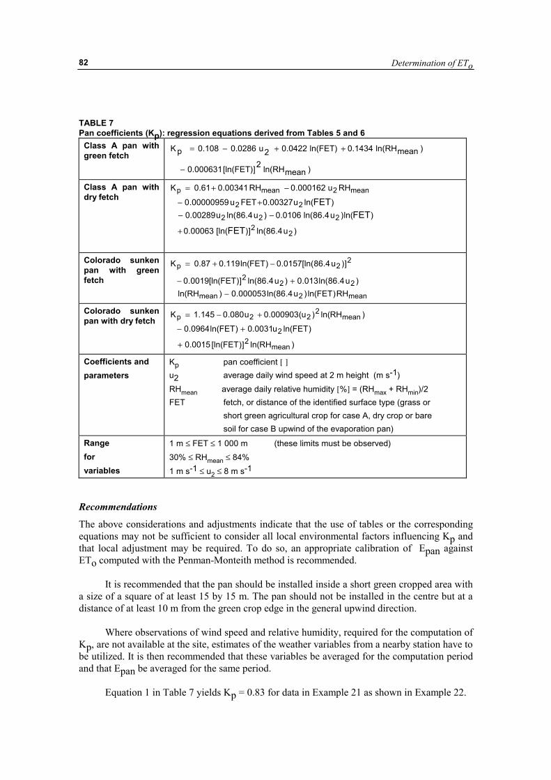
Determination of ETo
82
TABLE 7 Pan coefficients (Kp): regression equations derived from Tables 5 and 6
Class A pan with green fetch
)meanln(RH2[ln(FET)]0.000631
)meanln(RH0.1434ln(FET)0.04222u0.02860.108pK
−
++−=
Class A pan with dry fetch
)u4.86ln()][ln(00063.0
)ln()u4.86ln(0106.0)u4.86ln(u00289.0)ln(u00327.0FETu00000959.0
RHu000162.0RH00341.061.0K
22
222
22
mean2meanp
FET
FETFET
+
−−+−
−+=
Colorado sunken pan with green fetch
mean2mean
222
22p
RH)FETln()u4.86ln(000053.0)RHln()u4.86ln(013.0)u4.86ln()]FET[ln(0019.0
)]u4.86[ln(0157.0)FETln(119.087.0K
−+−
−+=
Colorado sunken pan with dry fetch
)RHln()]FET[ln(0015.0
)FETln(u0031.0)FETln(0964.0
)RHln()u(000903.0u080.0145.1K
mean2
2
mean2
22p
+
+−
+−=
Coefficients and parameters
Kp pan coefficient [ ] u2 average daily wind speed at 2 m height (m s-1) RHmean average daily relative humidity [%] = (RHmax + RHmin)/2 FET fetch, or distance of the identified surface type (grass or short green agricultural crop for case A, dry crop or bare soil for case B upwind of the evaporation pan)
Range for variables
1 m ≤ FET ≤ 1 000 m (these limits must be observed) 30% ≤ RHmean ≤ 84% 1 m s-1 ≤ u2 ≤ 8 m s-1
Recommendations
The above considerations and adjustments indicate that the use of tables or the corresponding equations may not be sufficient to consider all local environmental factors influencing Kp and that local adjustment may be required. To do so, an appropriate calibration of Epan against ETo computed with the Penman-Monteith method is recommended.
It is recommended that the pan should be installed inside a short green cropped area with a size of a square of at least 15 by 15 m. The pan should not be installed in the centre but at a distance of at least 10 m from the green crop edge in the general upwind direction.
Where observations of wind speed and relative humidity, required for the computation of Kp, are not available at the site, estimates of the weather variables from a nearby station have to be utilized. It is then recommended that these variables be averaged for the computation period and that Epan be averaged for the same period.
Equation 1 in Table 7 yields Kp = 0.83 for data in Example 21 as shown in Example 22.
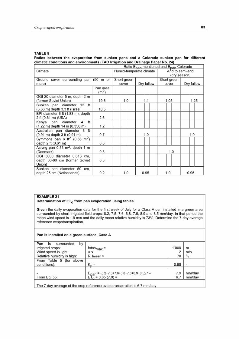
Crop evapotranspiration
83
TABLE 8 Ratios between the evaporation from sunken pans and a Colorado sunken pan for different climatic conditions and environments (FAO Irrigation and Drainage Paper No. 24)
Ratio Epan mentioned and Epan Colorado Climate Humid-temperate climate Arid to semi-arid
(dry season) Ground cover surrounding pan (50 m or more)
Short green cover
Dry fallow
Short green cover
Dry fallow
Pan area (m2)
GGI 20 diameter 5 m, depth 2 m (former Soviet Union)
19.6
1.0
1.1
1.05
1.25
Sunken pan diameter 12 ft (3.66 m) depth 3.3 ft (Israel)
10.5
BPI diameter 6 ft (1.83 m), depth 2 ft (0.61 m) (USA)
2.6
Kenya pan diameter 4 ft (1.22 m) depth 14 in (0.356 m)
1.2
Australian pan diameter 3 ft (0.91 m) depth 3 ft (0.91 m)
0.7
1.0
1.0
Symmons pan 6 ft2 (0.56 m2) depth 2 ft (0.61 m)
0.6
Aslyng pan 0.33 m2, depth 1 m (Denmark)
0.3
1.0
GGI 3000 diameter 0.618 cm, depth 60-80 cm (former Soviet Union)
0.3
Sunken pan diameter 50 cm, depth 25 cm (Netherlands)
0.2
1.0
0.95
1.0
0.95
EXAMPLE 21 Determination of ETo from pan evaporation using tables Given the daily evaporation data for the first week of July for a Class A pan installed in a green area surrounded by short irrigated field crops: 8.2, 7.5, 7.6, 6.8, 7.6, 8.9 and 8.5 mm/day. In that period the mean wind speed is 1.9 m/s and the daily mean relative humidity is 73%. Determine the 7-day average reference evapotranspiration. Pan is installed on a green surface: Case A Pan is surrounded by irrigated crops: Wind speed is light: Relative humidity is high:
fetchmax = u < RHmean >
1 000
2 70
m m/s %
From Table 5 (for above conditions):
Kp =
0.85
-
- From Eq. 55:
Epan = (8.2+7.5+7.6+6.8+7.6+8.9+8.5)/7 = ETo = 0.85 (7.9) =
7.9 6.7
mm/day mm/day
The 7-day average of the crop reference evapotranspiration is 6.7 mm/day
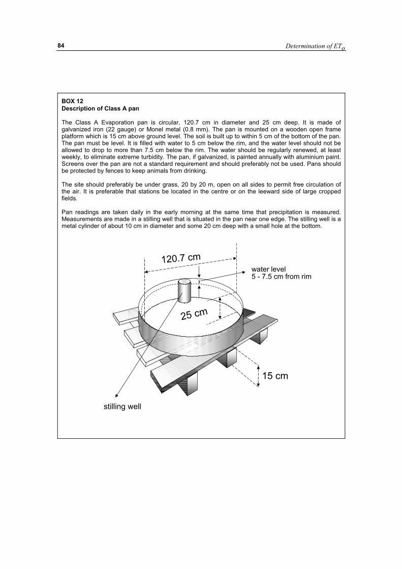
Determination of ETo
84
BOX 12 Description of Class A pan The Class A Evaporation pan is circular, 120.7 cm in diameter and 25 cm deep. It is made of galvanized iron (22 gauge) or Monel metal (0.8 mm). The pan is mounted on a wooden open frame platform which is 15 cm above ground level. The soil is built up to within 5 cm of the bottom of the pan. The pan must be level. It is filled with water to 5 cm below the rim, and the water level should not be allowed to drop to more than 7.5 cm below the rim. The water should be regularly renewed, at least weekly, to eliminate extreme turbidity. The pan, if galvanized, is painted annually with aluminium paint. Screens over the pan are not a standard requirement and should preferably not be used. Pans should be protected by fences to keep animals from drinking. The site should preferably be under grass, 20 by 20 m, open on all sides to permit free circulation of the air. It is preferable that stations be located in the centre or on the leeward side of large cropped fields. Pan readings are taken daily in the early morning at the same time that precipitation is measured. Measurements are made in a stilling well that is situated in the pan near one edge. The stilling well is a metal cylinder of about 10 cm in diameter and some 20 cm deep with a small hole at the bottom.
120.7 cm
15 cm
25 cm
stilling well
water level5 - 7.5 cm from rim

Crop evapotranspiration
85
BOX 13 Description of Colorado sunken pan The Colorado sunken pan is 92 cm (3 ft) square and 46 cm (18 in) deep, made of 3 mm thick iron, placed in the ground with the rim 5 cm (2 in) above the soil level. Also, the dimensions 1 m square and 0.5 m deep are frequently used. The pan is painted with black tar paint. The water level is maintained at or slightly below ground level, i.e., 5-7.5 cm below the rim. Measurements are taken similarly to those for the Class A pan. Siting and environment requirements are also similar to those for the Class A pan. Sunken Colorado pans are sometimes preferred in crop water requirements studies, as these pans give a better direct estimation of the reference evapotranspiration than does the Class A pan. The disadvantage is that maintenance is more difficult and leaks are not visible.
5 cm
46 cm
92 cm 92 cm
water level5 - 7.5 cm from rim
stilling well
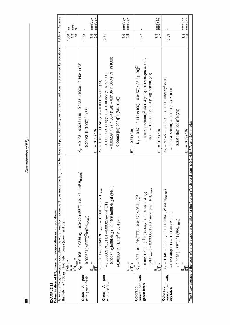
D
eter
min
atio
n of
ET o
86 EX
AMPL
E 22
D
eter
min
atio
n of
ET o
from
pan
eva
pora
tion
usin
g eq
uatio
ns
Giv
en th
e 7-
day
aver
age
evap
orat
ion
mea
sure
men
t fro
m E
xam
ple
21, e
stim
ate
the
ETo fo
r the
two
type
s of
pan
s an
d tw
o ty
pes
of fe
tch
cond
ition
s re
pres
ente
d by
equ
atio
ns in
Tab
le 7
. As
sum
e th
at fe
tch
is 1
000
m in
bot
h fe
tch
case
s (g
reen
and
dry
).
Fetc
h =
u 2 =
RH
mea
n =
10
00
1.9 73
m
m/s
%
C
lass
A
pan
with
gre
en fe
tch
)R
Hln
()]
FET
[ln(
0006
31.0
)R
Hln
(14
34.0
)FE
Tln
(04
22.0
u02
86.0
108
.0K
mea
n2
mea
n2
p −
++
−=
E pan =
ET
o =
)73
ln(
)]10
00[ln
(00
0631
.0
)73
ln(
1434
.0)
1000
ln(
0422
.0)9.1(
0286
.010
8.0
K2
p −
++
−=
ETo =
0.8
3 (7
.9)
0.
83
7.9
6.6
- mm
/day
m
m/d
ay
Cla
ss
A pa
n w
ith d
ry fe
tch
)u4.
86ln
()]
[ln(
0006
3.0
)ln
()
u4.86
ln(
0106
.0)
u4.86
ln(
u00
289
.0)
ln(
u00
327
.0FE
Tu
0000
0959
.0
RH
u00
0162
.0R
H00
341
.061.0
K
22
22
2
22
mea
n2
mea
np
FET
FET
FET
+
−−
+−
−+
=
E pan =
ET
o =
))9.1(4.
86ln
()]
1000
[ln(
0006
3.0
)10
00ln
())9.1(
4.86
ln(
0106
.0))9.1(
4.86
ln(
)9.1(00
289
.0)
1000
ln(
)9.1(00
327
.0)
1000
()9.1(00
0009
59.0
)73()9.1(
0001
62.0
)73(
0034
1.0
61.0K
2
p +
−−
+−
−+
=
ETo =
0.6
1 (7
.9)
0.
61
7.9
4.8
- mm
/day
m
m/d
ay
Col
orad
o su
nken
pan
with
gr
een
fetc
h
mea
n2
mea
n
22
2
22
p
RH
)FE
Tln
()
u4.86
ln(
0000
53.0
)R
Hln
()
u4.86
ln(
013
.0)
u4.86
ln(
)]FE
T[ln
(00
19.0
)]u4.
86[ln
(01
57.0
)FE
Tln
(11
9.0
87.0K
−+
−
−+
=
E pan =
ET
o =
)73()
1000
ln(
))9.1(4.
86ln
(00
0053
.0)
73ln
())9.1(
4.86
ln(
013
.0))9.1(
4.86
ln(
)]10
00[ln
(00
19.0
))]9.1(4.
86[ln
(01
57.0
)10
0ln
(11
9.0
87.0K
2
2p
−+
−
−+
=
ET
o = 0
.97
(7.9
)
0.97
7.
9 7.
7
- m
m/d
ay
mm
/day
C
olor
ado
sunk
en p
an w
ith
dry
fetc
h
)R
Hln
()]
FET
[ln(
0015
.0
)FE
Tln
(u
0031
.0)
FET
ln(
0964
.0
)R
Hln
()
u(00
0903
.0u
080
.014
5.1
K
mea
n2
2
mea
n2
22
p +
+−
+−
=
E pan =
ET
o =
)73
ln(
)]10
00[ln
(00
15.0
)10
00ln
()9.1(
0031
.0)
1000
ln(
0964
.0
)73
ln(
)9.1(00
0903
.0)9.1(
080
.014
5.1
K
2
2p +
+−
+−
=
ETo =
0.6
9 (7
.9)
0.
69
7.9
5.4
- mm
/day
m
m/d
ay
The
7-da
y av
erag
e of
the
crop
refe
renc
e ev
apot
rans
pira
tion
for t
he fo
ur p
an/fe
tch
cond
ition
s is
6.6
, 4.8
, 7.7
, and
5.4
mm
/day
Crop evapotranspiration
87
Part B
Crop evapotranspiration under standard conditions
This part examines crop evapotranspiration under standard conditions (ETc). This is the evapotranspiration from disease-free, well-fertilized crops, grown in large fields, under optimum soil water conditions and achieving full production under the given climatic conditions. The effects of various weather conditions on evapotranspiration are incorporated into ETo (Part A). The effects of characteristics that distinguish the cropped surface from the reference surface are integrated into the crop coefficient. By multiplying ETo by the crop coefficient, ETc is determined. Typical crop coefficients, calculation procedures for adjusting the crop coefficients and for calculating ETc are presented in this part. Two calculation approaches are outlined: the single and the dual crop coefficient approach. In the single crop coefficient approach, the difference in evapotranspiration between the cropped and reference grass is combined into one single coefficient. In the dual crop coefficient approach, the crop coefficient is split into two factors describing separately the differences in evaporation and transpiration between the crop and reference surface. As discussed in Chapter 5 and summarized in Table 10, the single crop coefficient approach is used for most applications related to irrigation planning, design, and management. The dual crop coefficient approach is relevant in calculations where detailed estimates of soil water evaporation are required, such as in real time irrigation scheduling applications, water quality modelling, and in research.

88
Crop evapotranspiration
89
Chapter 5
Introduction to crop evapotranspiration (ETc)
This chapter outlines the crop coefficient approach for calculating the crop evapotranspiration under standard conditions (ETc). The standard conditions refer to crops grown in large fields under excellent agronomic and soil water conditions. The crop evapotranspiration differs distinctly from the reference evapotranspiration (ETo) as the ground cover, canopy properties and aerodynamic resistance of the crop are different from grass. The effects of characteristics that distinguish field crops from grass are integrated into the crop coefficient (Kc). In the crop coefficient approach, crop evapotranspiration is calculated by multiplying ETo by Kc.
Differences in evaporation and transpiration between field crops and the reference grass surface can be integrated in a single crop coefficient (Kc) or separated into two coefficients: a basal crop (Kcb) and a soil evaporation coefficient (Ke), i.e., Kc = Kcb + Ke. The approach to follow should be selected as a function of the purpose of the calculation, the accuracy required and the data available. CALCULATION PROCEDURES Direct calculation The evapotranspiration rate from a cropped surface can be directly measured by the mass transfer or the energy balance method. It can also be derived from studies of the soil water balance determined from cropped fields or from lysimeters.
Crop evapotranspiration can also be derived from meteorological and crop data by means of the Penman-Monteith equation (Eq. 3). By adjusting the albedo and the aerodynamic and canopy surface resistances to the growing characteristics of the specific crop, the evapotranspiration rate can be directly estimated. The albedo and resistances are, however, difficult to estimate accurately as they may vary continually during the growing season as climatic conditions change, as the crop develops, and with wetness of the soil surface. The canopy resistance will further be influenced by the soil water availability, and it increases strongly if the crop is subjected to water stress.
As there is still a considerable lack of consolidated information on the aerodynamic and canopy resistances for the various cropped surfaces, the FAO Penman-Monteith method is used in this handbook only for estimating ETo, the evapotranspiration from a well-watered hypothetical grass surface having fixed crop height, albedo and surface resistance.
Introduction to crop evapotranspiration (ETc)
90
Crop coefficient approach In the crop coefficient approach the crop evapotranspiration, ETc, is calculated by multiplying the reference crop evapotranspiration, ETo, by a crop coefficient, Kc:
occ ETKET = (56) where ETc crop evapotranspiration [mm d-1],
Kc crop coefficient [dimensionless], ETo reference crop evapotranspiration [mm d-1].
Most of the effects of the various weather conditions are incorporated into the ETo
estimate. Therefore, as ETo represents an index of climatic demand, Kc varies predominately with the specific crop characteristics and only to a limited extent with climate. This enables the transfer of standard values for Kc between locations and between climates. This has been a primary reason for the global acceptance and usefulness of the crop coefficient approach and the Kc factors developed in past studies.
The reference ETo is defined and calculated using the FAO Penman-Monteith equation (Chapter 4). The crop coefficient, Kc, is basically the ratio of the crop ETc to the reference ETo, and it represents an integration of the effects of four primary characteristics that distinguish the crop from reference grass. These characteristics are:
• Crop height. The crop height influences the aerodynamic resistance term, ra, of the FAO Penman-Monteith equation and the turbulent transfer of vapour from the crop into the atmosphere. The ra term appears twice in the full form of the FAO Penman-Monteith equation.
• Albedo (reflectance) of the crop-soil surface. The albedo is affected by the fraction of ground covered by vegetation and by the soil surface wetness. The albedo of the crop-soil surface influences the net radiation of the surface, Rn, which is the primary source of the energy exchange for the evaporation process.
• Canopy resistance. The resistance of the crop to vapour transfer is affected by leaf area (number of stomata), leaf age and condition, and the degree of stomatal control. The canopy resistance influences the surface resistance, rs.
• Evaporation from soil, especially exposed soil.
The soil surface wetness and the fraction of ground covered by vegetation influence the surface resistance, rs. Following soil wetting, the vapour transfer rate from the soil is high, especially for crops having incomplete ground cover. The combined surface resistance of the canopy and of the soil determines the (bulk) surface resistance, rs. The surface resistance term in the Penman-Monteith equation represents the resistance to vapour flow from within plant leaves and from beneath the soil surface.
The Kc in Equation 56 predicts ETc under standard conditions. This represents the upper envelope of crop evapotranspiration and represents conditions where no limitations are placed on crop growth or evapotranspiration due to water shortage, crop density, or disease, weed, insect or salinity pressures. The ETc predicted by Kc is adjusted if necessary to non-standard
Crop evapotranspiration
91
conditions, ETc adj, where any environmental condition or characteristic is known to have an impact on or to limit ETc. Factors for correcting ETc to ETc adj are described in Part C. FACTORS DETERMINING THE CROP COEFFICIENT The crop coefficient integrates the effect of characteristics that distinguish a typical field crop from the grass reference, which has a constant appearance and a complete ground cover. Consequently, different crops will have different Kc coefficients. The changing characteristics of the crop over the growing season also affect the Kc coefficient. Finally, as evaporation is an integrated part of crop evapotranspiration, conditions affecting soil evaporation will also have an effect on Kc. Crop type Due to differences in albedo, crop height, aerodynamic properties, and leaf and stomata properties, the evapotranspiration from full grown, well-watered crops differs from ETo.
The close spacings of plants and taller canopy height and roughness of many full grown agricultural crops cause these crops to have Kc factors that are larger than 1. The Kc factor is often 5-10% higher than the reference (where Kc = 1.0), and even 15-20% greater for some tall crops such as maize, sorghum or sugar cane (Figure 20). Typical values for the crop coefficient for full grown crops (Kc mid) are listed in Table 12.
Crops such as pineapples, that close their stomata during the day, have very small crop coefficients. In most species, however, the stomata open as irradiance increases. In addition to the stomatal response to environment, the position and number of the stomata and the resistance of the cuticula to vapour transfer determine the water loss from the crop. Species with stomata on only the lower side of the leaf and/or large leaf resistances will have relatively smaller Kc values. This is the case for citrus and most deciduous fruit trees. Transpiration control and spacing of the trees, providing only 70% ground cover for mature trees, may cause the Kc of those trees, if cultivated without a ground cover crop, to be smaller than one (Figure 20). Climate The Kc values of Table 12 are typical values expected for average Kc under a standard climatic condition, which is defined as a sub-humid climate with average daytime minimum relative humidity (RHmin) ≈ 45% and having calm to moderate wind speeds averaging 2 m/s. Variations in wind alter the aerodynamic resistance of the crops and hence their crop coefficients, especially for those crops that are substantially taller than the hypothetical grass reference. The effect of the difference in aerodynamic properties between the grass reference surface and agricultural crops is not only crop specific. It also varies with the climatic conditions and crop height. Because aerodynamic properties are greater for many agricultural crops as compared to the grass reference, the ratio of ETc to ETo (i.e., Kc) for many crops increases as wind speed increases and as relative humidity decreases. More arid climates and conditions of greater wind speed will have higher values for Kc. More humid climates and conditions of lower wind speed will have lower values for Kc.
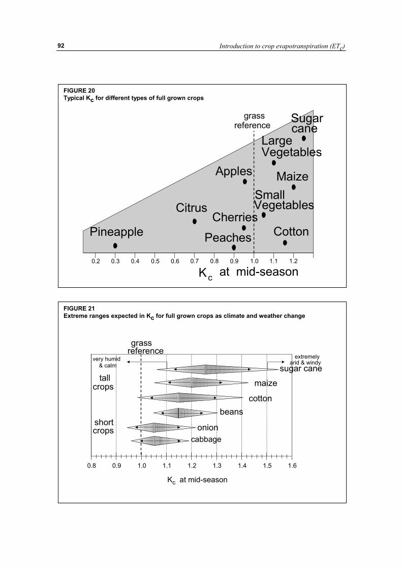
Introduction to crop evapotranspiration (ETc)
92
FIGURE 20 Typical Kc for different types of full grown crops
0.2 0.3 0.4 0.5 0.6 0.7 0.8 0.9 1.0 1.1 1.2
reference
Kc
Pineapple
Citrus
Peaches Cotton
SmallVegetables
Maize
Sugarcane
LargeVegetables
Apples
Cherries
grass
at mid-season
FIGURE 21 Extreme ranges expected in Kc for full grown crops as climate and weather change
0.8 0.9 1.0 1.1 1.2 1.3 1.4 1.5 1.6
Kc at mid-season
cabbage
extremelyarid & windyvery humid
& calm
cotton
maize
sugar canetall
crops
crops
grassreference
shortbeans
onion
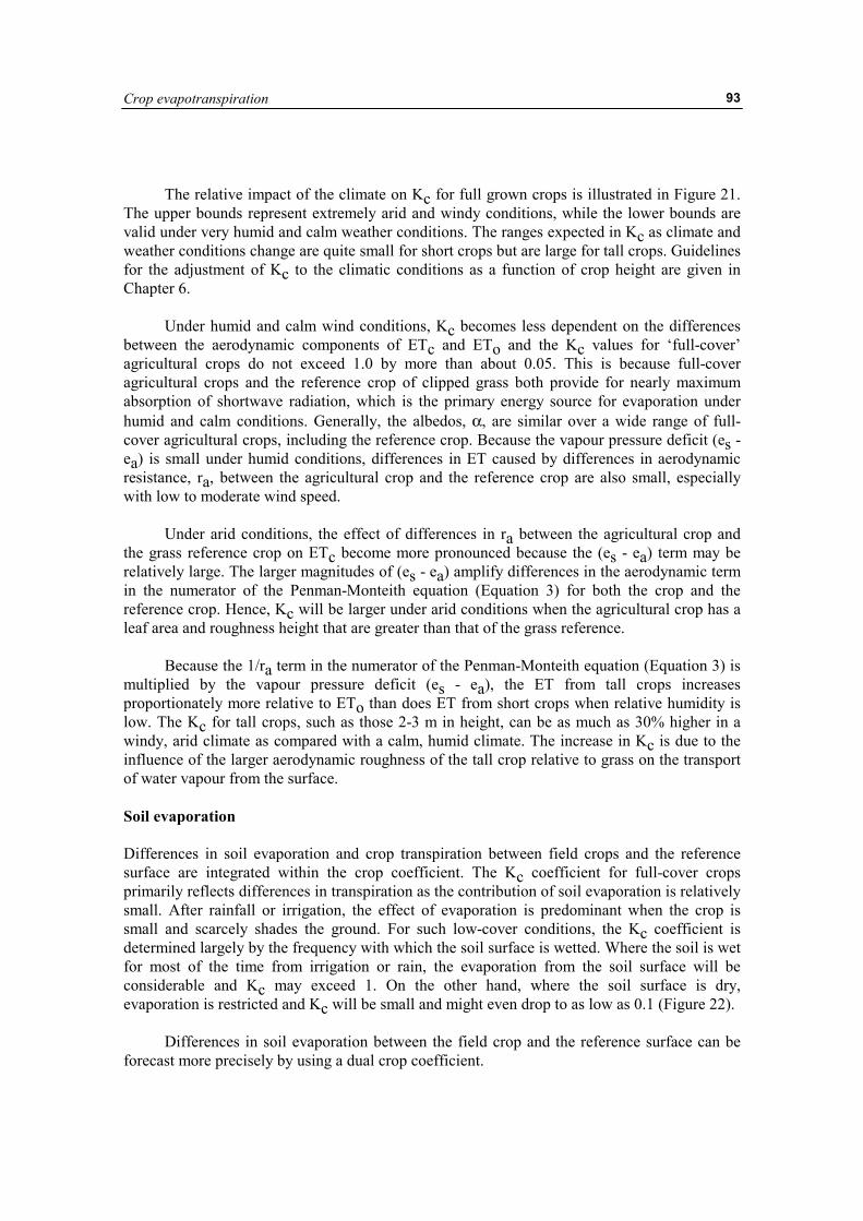
Crop evapotranspiration
93
The relative impact of the climate on Kc for full grown crops is illustrated in Figure 21. The upper bounds represent extremely arid and windy conditions, while the lower bounds are valid under very humid and calm weather conditions. The ranges expected in Kc as climate and weather conditions change are quite small for short crops but are large for tall crops. Guidelines for the adjustment of Kc to the climatic conditions as a function of crop height are given in Chapter 6.
Under humid and calm wind conditions, Kc becomes less dependent on the differences between the aerodynamic components of ETc and ETo and the Kc values for ‘full-cover’ agricultural crops do not exceed 1.0 by more than about 0.05. This is because full-cover agricultural crops and the reference crop of clipped grass both provide for nearly maximum absorption of shortwave radiation, which is the primary energy source for evaporation under humid and calm conditions. Generally, the albedos, α, are similar over a wide range of full-cover agricultural crops, including the reference crop. Because the vapour pressure deficit (es - ea) is small under humid conditions, differences in ET caused by differences in aerodynamic resistance, ra, between the agricultural crop and the reference crop are also small, especially with low to moderate wind speed.
Under arid conditions, the effect of differences in ra between the agricultural crop and the grass reference crop on ETc become more pronounced because the (es - ea) term may be relatively large. The larger magnitudes of (es - ea) amplify differences in the aerodynamic term in the numerator of the Penman-Monteith equation (Equation 3) for both the crop and the reference crop. Hence, Kc will be larger under arid conditions when the agricultural crop has a leaf area and roughness height that are greater than that of the grass reference.
Because the 1/ra term in the numerator of the Penman-Monteith equation (Equation 3) is multiplied by the vapour pressure deficit (es - ea), the ET from tall crops increases proportionately more relative to ETo than does ET from short crops when relative humidity is low. The Kc for tall crops, such as those 2-3 m in height, can be as much as 30% higher in a windy, arid climate as compared with a calm, humid climate. The increase in Kc is due to the influence of the larger aerodynamic roughness of the tall crop relative to grass on the transport of water vapour from the surface. Soil evaporation Differences in soil evaporation and crop transpiration between field crops and the reference surface are integrated within the crop coefficient. The Kc coefficient for full-cover crops primarily reflects differences in transpiration as the contribution of soil evaporation is relatively small. After rainfall or irrigation, the effect of evaporation is predominant when the crop is small and scarcely shades the ground. For such low-cover conditions, the Kc coefficient is determined largely by the frequency with which the soil surface is wetted. Where the soil is wet for most of the time from irrigation or rain, the evaporation from the soil surface will be considerable and Kc may exceed 1. On the other hand, where the soil surface is dry, evaporation is restricted and Kc will be small and might even drop to as low as 0.1 (Figure 22).
Differences in soil evaporation between the field crop and the reference surface can be forecast more precisely by using a dual crop coefficient.
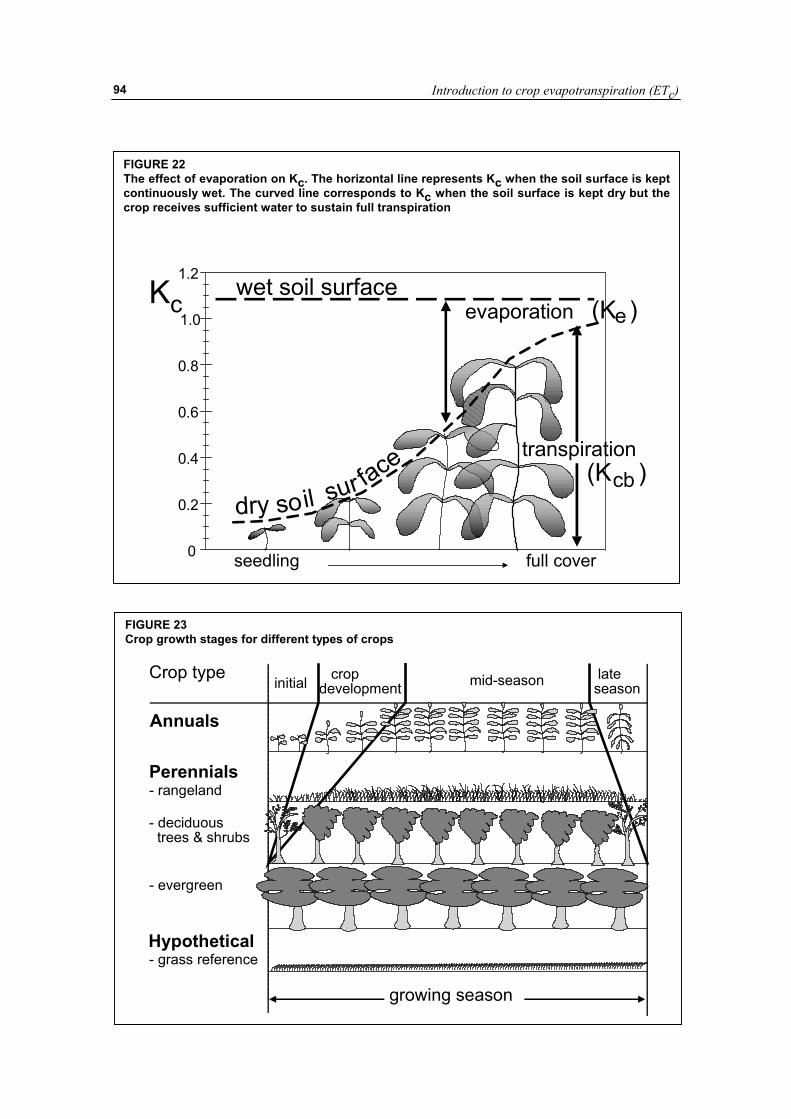
Introduction to crop evapotranspiration (ETc)
94
FIGURE 22 The effect of evaporation on Kc. The horizontal line represents Kc when the soil surface is kept continuously wet. The curved line corresponds to Kc when the soil surface is kept dry but the crop receives sufficient water to sustain full transpiration
0
0.2
0.4
0.6
0.8
1.0
1.2
seedling full cover
dry soil
evaporation
transpiration
Kcwet soil surface
sur face cb
(K )e
(K )
FIGURE 23 Crop growth stages for different types of crops
initial lateseason
Crop type
- rangeland
- deciduous trees & shrubs
- evergreen
- grass reference
growing season
mid-season
Hypothetical
Annuals
Perennials
cropdevelopment
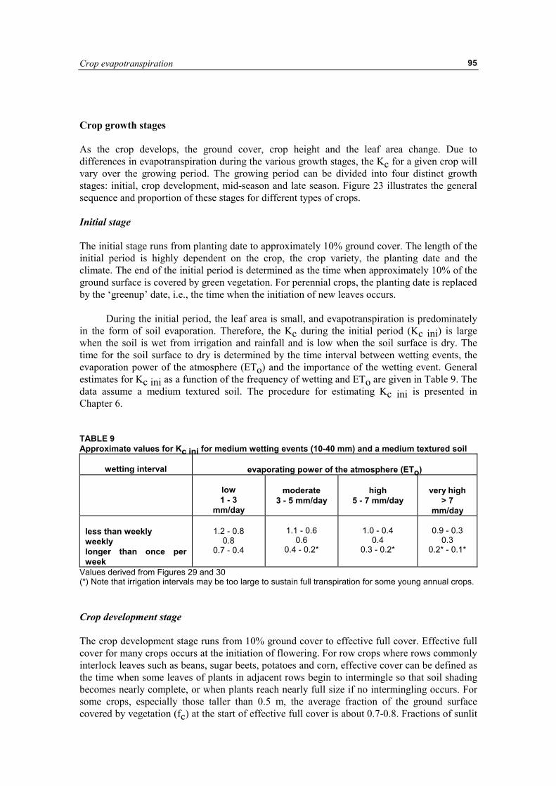
Crop evapotranspiration
95
Crop growth stages As the crop develops, the ground cover, crop height and the leaf area change. Due to differences in evapotranspiration during the various growth stages, the Kc for a given crop will vary over the growing period. The growing period can be divided into four distinct growth stages: initial, crop development, mid-season and late season. Figure 23 illustrates the general sequence and proportion of these stages for different types of crops. Initial stage The initial stage runs from planting date to approximately 10% ground cover. The length of the initial period is highly dependent on the crop, the crop variety, the planting date and the climate. The end of the initial period is determined as the time when approximately 10% of the ground surface is covered by green vegetation. For perennial crops, the planting date is replaced by the ‘greenup’ date, i.e., the time when the initiation of new leaves occurs.
During the initial period, the leaf area is small, and evapotranspiration is predominately in the form of soil evaporation. Therefore, the Kc during the initial period (Kc ini) is large when the soil is wet from irrigation and rainfall and is low when the soil surface is dry. The time for the soil surface to dry is determined by the time interval between wetting events, the evaporation power of the atmosphere (ETo) and the importance of the wetting event. General estimates for Kc ini as a function of the frequency of wetting and ETo are given in Table 9. The data assume a medium textured soil. The procedure for estimating Kc ini is presented in Chapter 6. TABLE 9 Approximate values for Kc ini for medium wetting events (10-40 mm) and a medium textured soil
wetting interval
evaporating power of the atmosphere (ETo)
low 1 - 3
mm/day
moderate
3 - 5 mm/day
high
5 - 7 mm/day
very high
> 7 mm/day
less than weekly weekly longer than once per week
1.2 - 0.8
0.8 0.7 - 0.4
1.1 - 0.6
0.6 0.4 - 0.2*
1.0 - 0.4
0.4 0.3 - 0.2*
0.9 - 0.3
0.3 0.2* - 0.1*
Values derived from Figures 29 and 30 (*) Note that irrigation intervals may be too large to sustain full transpiration for some young annual crops. Crop development stage The crop development stage runs from 10% ground cover to effective full cover. Effective full cover for many crops occurs at the initiation of flowering. For row crops where rows commonly interlock leaves such as beans, sugar beets, potatoes and corn, effective cover can be defined as the time when some leaves of plants in adjacent rows begin to intermingle so that soil shading becomes nearly complete, or when plants reach nearly full size if no intermingling occurs. For some crops, especially those taller than 0.5 m, the average fraction of the ground surface covered by vegetation (fc) at the start of effective full cover is about 0.7-0.8. Fractions of sunlit
Introduction to crop evapotranspiration (ETc)
96
and shaded soil and leaves do not change significantly with further growth of the crop beyond fc ≈ 0.7 to 0.8. It is understood that the crop or plant can continue to grow in both height and leaf area after the time of effective full cover. Because it is difficult to visually determine when densely sown vegetation such as winter and spring cereals and some grasses reach effective full cover, the more easily detectable stage of heading (flowering) is generally used for these types of crops.
For dense grasses, effective full cover may occur at about 0.10-0.15 m height. For thin stands of grass (dry rangeland), grass height may approach 0.3-0.5 m before effective full cover is reached. Densely planted forages such as alfalfa and clover reach effective full cover at about 0.3-0.4 m.
Another way to estimate the occurrence of effective full cover is when the leaf area index (LAI) reaches three. LAI is defined as the average total area of leaves (one side) per unit area of ground surface.
As the crop develops and shades more and more of the ground, evaporation becomes more restricted and transpiration gradually becomes the major process. During the crop development stage, the Kc value corresponds to amounts of ground cover and plant development. Typically, if the soil surface is dry, Kc = 0.5 corresponds to about 25-40% of the ground surface covered by vegetation due to the effects of shading and due to microscale transport of sensible heat from the soil into the vegetation. A Kc = 0.7 often corresponds to about 40-60% ground cover. These values will vary, depending on the crop, frequency of wetting and whether the crop uses more water than the reference crop at full ground cover (e.g., depending on its canopy architecture and crop height relative to clipped grass). Mid-season stage The mid-season stage runs from effective full cover to the start of maturity. The start of maturity is often indicated by the beginning of the ageing, yellowing or senescence of leaves, leaf drop, or the browning of fruit to the degree that the crop evapotranspiration is reduced relative to the reference ETo. The mid-season stage is the longest stage for perennials and for many annuals, but it may be relatively short for vegetable crops that are harvested fresh for their green vegetation.
At the mid-season stage the Kc reaches its maximum value. The value for Kc (Kc mid) is relatively constant for most growing and cultural conditions. Deviation of the Kc mid from the reference value '1' is primarily due to differences in crop height and resistance between the grass reference surface and the agricultural crop and weather conditions. Late season stage The late season stage runs from the start of maturity to harvest or full senescence. The calculation for Kc and ETc is presumed to end when the crop is harvested, dries out naturally, reaches full senescence, or experiences leaf drop.
For some perennial vegetation in frost free climates, crops may grow year round so that the date of termination may be taken as the same as the date of ‘planting’.
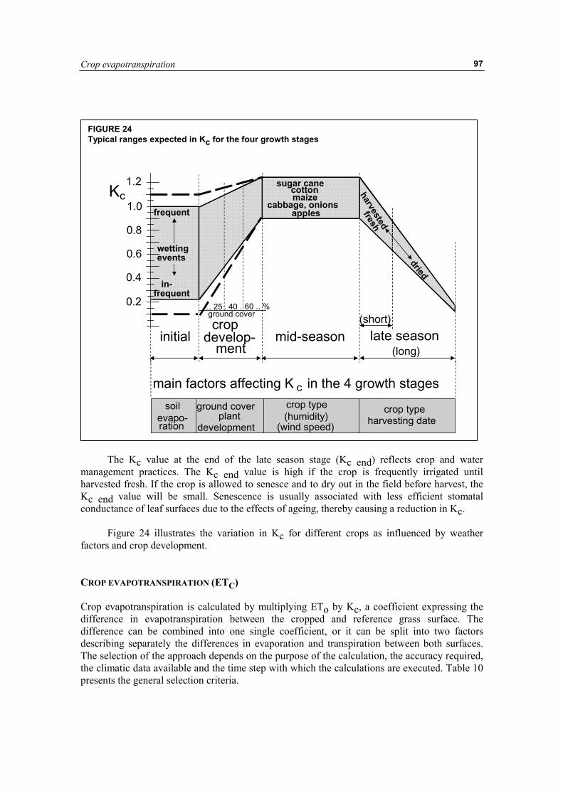
Crop evapotranspiration
97
The Kc value at the end of the late season stage (Kc end) reflects crop and water
management practices. The Kc end value is high if the crop is frequently irrigated until harvested fresh. If the crop is allowed to senesce and to dry out in the field before harvest, the Kc end value will be small. Senescence is usually associated with less efficient stomatal conductance of leaf surfaces due to the effects of ageing, thereby causing a reduction in Kc.
Figure 24 illustrates the variation in Kc for different crops as influenced by weather factors and crop development. CROP EVAPOTRANSPIRATION (ETC) Crop evapotranspiration is calculated by multiplying ETo by Kc, a coefficient expressing the difference in evapotranspiration between the cropped and reference grass surface. The difference can be combined into one single coefficient, or it can be split into two factors describing separately the differences in evaporation and transpiration between both surfaces. The selection of the approach depends on the purpose of the calculation, the accuracy required, the climatic data available and the time step with which the calculations are executed. Table 10 presents the general selection criteria.
FIGURE 24 Typical ranges expected in Kc for the four growth stages
1.0 frequent
in-frequent
sugar canecottonmaize
cabbage, onionsapples
harvested
fresh
dried
wettingevents
0.8
0.6
0.4
0.2
1.2Kc
(short)
(long)mid-season late seasoninitial
crop
mentdevelop-
60 .. %.. 25ground cover
. 40 .
csoil ground cover crop type
evapo-ration
plantdevelopment (wind speed)
(humidity)
main factors affecting K
crop typeharvesting date
in the 4 growth stages
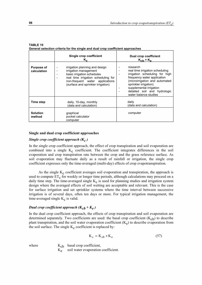
Introduction to crop evapotranspiration (ETc)
98
TABLE 10 General selection criteria for the single and dual crop coefficient approaches
Single crop coefficient
Kc
Dual crop coefficient
Kcb + Ke Purpose of calculation
- irrigation planning and design - irrigation management - basic irrigation schedules - real time irrigation scheduling for non-frequent water applications (surface and sprinkler irrigation)
- research - real time irrigation scheduling - irrigation scheduling for high frequency water application (microirrigation and automated sprinkler irrigation) - supplemental irrigation - detailed soil and hydrologic water balance studies
Time step
daily, 10-day, monthly (data and calculation)
daily (data and calculation)
Solution method
graphical pocket calculator computer
computer
Single and dual crop coefficient approaches
Single crop coefficient approach (Kc )
In the single crop coefficient approach, the effect of crop transpiration and soil evaporation are combined into a single Kc coefficient. The coefficient integrates differences in the soil evaporation and crop transpiration rate between the crop and the grass reference surface. As soil evaporation may fluctuate daily as a result of rainfall or irrigation, the single crop coefficient expresses only the time-averaged (multi-day) effects of crop evapotranspiration.
As the single Kc coefficient averages soil evaporation and transpiration, the approach is used to compute ETc for weekly or longer time periods, although calculations may proceed on a daily time step. The time-averaged single Kc is used for planning studies and irrigation system design where the averaged effects of soil wetting are acceptable and relevant. This is the case for surface irrigation and set sprinkler systems where the time interval between successive irrigation is of several days, often ten days or more. For typical irrigation management, the time-averaged single Kc is valid. Dual crop coefficient approach (Kcb + Ke )
In the dual crop coefficient approach, the effects of crop transpiration and soil evaporation are determined separately. Two coefficients are used: the basal crop coefficient (Kcb) to describe plant transpiration, and the soil water evaporation coefficient (Ke) to describe evaporation from the soil surface. The single Kc coefficient is replaced by:
ecbc KKK += (57) where Kcb basal crop coefficient,
Ke soil water evaporation coefficient.
Crop evapotranspiration
99
The basal crop coefficient, Kcb, is defined as the ratio of ETc to ETo when the soil surface layer is dry but where the average soil water content of the root zone is adequate to sustain full plant transpiration. The Kcb represents the baseline potential Kc in the absence of the additional effects of soil wetting by irrigation or precipitation. The soil evaporation coefficient, Ke, describes the evaporation component from the soil surface. If the soil is wet following rain or irrigation, Ke may be large. However, the sum of Kcb and Ke can never exceed a maximum value, Kc max, determined by the energy available for evapotranspiration at the soil surface. As the soil surface becomes drier, Ke becomes smaller and falls to zero when no water is left for evaporation. The estimation of Ke requires a daily water balance computation for the calculation of the soil water content remaining in the upper topsoil.
The dual coefficient approach requires more numerical calculations than the procedure using the single time-averaged Kc coefficient. The dual procedure is best for real time irrigation scheduling, for soil water balance computations, and for research studies where effects of day-to-day variations in soil surface wetness and the resulting impacts on daily ETc, the soil water profile, and deep percolation fluxes are important. This is the case for high frequency irrigation with microirrigation systems or lateral move systems such as centre pivots and linear move systems. Crop coefficient curve After the selection of the calculation approach, the determination of the lengths for the crop growth stages and the corresponding crop coefficients, a crop coefficient curve can be constructed. The curve represents the changes in the crop coefficient over the length of the growing season. The shape of the curve represents the changes in the vegetation and ground cover during plant development and maturation that affect the ratio of ETc to ETo. From the curve, the Kc factor and hence ETc can be derived for any period within the growing season. Single crop coefficient The generalized crop coefficient curve is shown in Figure 25. Shortly after the planting of annuals or shortly after the initiation of new leaves for perennials, the value for Kc is small, often less than 0.4. The Kc begins to increase from the initial Kc value, Kc ini, at the beginning of rapid plant development and reaches a maximum value, Kc mid, at the time of maximum or near maximum plant development. During the late season period, as leaves begin to age and senesce due to natural or cultural practices, the Kc begins to decrease until it reaches a lower value at the end of the growing period equal to Kc end. Dual crop coefficient The single 'time-averaged' Kc curve in Figure 25 incorporates averaged wetting effects into the Kc factor. The value for Kc mid is relatively constant for most growing and cultural conditions. However, the values for Kc ini and Kc end can vary considerably on a daily basis, depending on the frequency of wetting by irrigation and rainfall. The dual crop coefficient approach calculates the actual increases in Kc for each day as a function of plant development and the wetness of the soil surface.
As the single Kc coefficient includes averaged effects of evaporation from the soil, the basal crop coefficient, Kcb d escribing only plant transpiration, lies below the Kc value (Figure
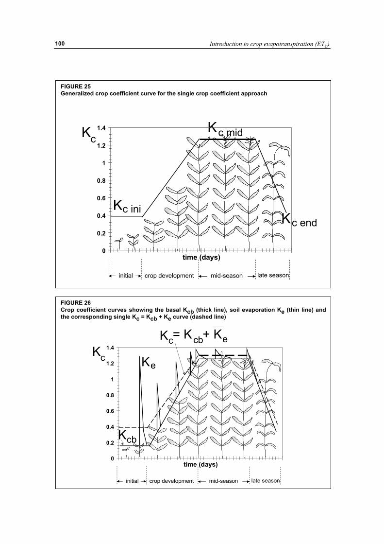
Introduction to crop evapotranspiration (ETc)
100
FIGURE 25 Generalized crop coefficient curve for the single crop coefficient approach
Kc
KK
K
c ini
c mid
c end
initial crop development mid-season late season
0
0.2
0.4
0.6
0.8
1
1.2
1.4
time (days)
FIGURE 26 Crop coefficient curves showing the basal Kcb (thick line), soil evaporation Ke (thin line) and the corresponding single Kc = Kcb + Ke curve (dashed line)
Kc
initial crop development mid-season late season
0
0.2
0.4
0.6
0.8
1
1.2
1.4
time (days)
K
cb
cb
K
Ke
= K + Kec
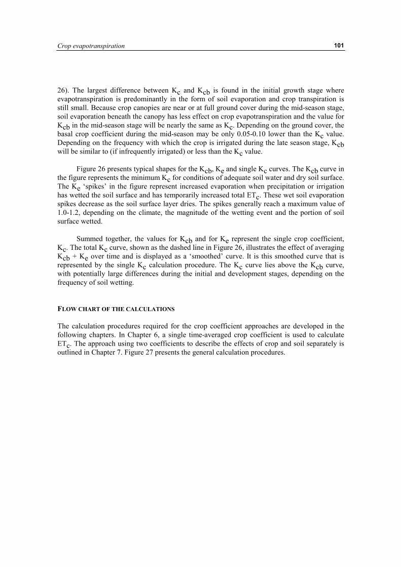
Crop evapotranspiration
101
26). The largest difference between Kc and Kcb is found in the initial growth stage where evapotranspiration is predominantly in the form of soil evaporation and crop transpiration is still small. Because crop canopies are near or at full ground cover during the mid-season stage, soil evaporation beneath the canopy has less effect on crop evapotranspiration and the value for Kcb in the mid-season stage will be nearly the same as Kc. Depending on the ground cover, the basal crop coefficient during the mid-season may be only 0.05-0.10 lower than the Kc value. Depending on the frequency with which the crop is irrigated during the late season stage, Kcb will be similar to (if infrequently irrigated) or less than the Kc value.
Figure 26 presents typical shapes for the Kcb, Ke and single Kc curves. The Kcb curve in the figure represents the minimum Kc for conditions of adequate soil water and dry soil surface. The Ke ‘spikes’ in the figure represent increased evaporation when precipitation or irrigation has wetted the soil surface and has temporarily increased total ETc. These wet soil evaporation spikes decrease as the soil surface layer dries. The spikes generally reach a maximum value of 1.0-1.2, depending on the climate, the magnitude of the wetting event and the portion of soil surface wetted.
Summed together, the values for Kcb and for Ke represent the single crop coefficient, Kc. The total Kc curve, shown as the dashed line in Figure 26, illustrates the effect of averaging Kcb + Ke over time and is displayed as a ‘smoothed’ curve. It is this smoothed curve that is represented by the single Kc calculation procedure. The Kc curve lies above the Kcb curve, with potentially large differences during the initial and development stages, depending on the frequency of soil wetting. FLOW CHART OF THE CALCULATIONS The calculation procedures required for the crop coefficient approaches are developed in the following chapters. In Chapter 6, a single time-averaged crop coefficient is used to calculate ETc. The approach using two coefficients to describe the effects of crop and soil separately is outlined in Chapter 7. Figure 27 presents the general calculation procedures.
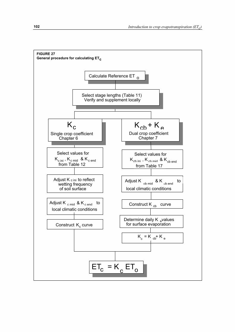
Introduction to crop evapotranspiration (ETc)
102
FIGURE 27 General procedure for calculating ETc
Calculate Reference ET
K K + K
ET = K ET
Construct Kc curve
K = K + K
o
c cb e
c ini c mid c end
Select values forK , K & K
c ini
c mid c endAdjust Klocal climatic conditions
to
Determine daily K values for surface evaporation
cb ini cb mid cb end
Select values forK , K & K
cb mid cb endAdjust K & K to
local climatic conditions
cbConstruct K curve
e
c cb e
c c o
& K
Adjust K to reflect wetting frequency of soil surface
Single crop coefficient Chapter 6
Dual crop coefficient Chapter 7
Select stage lengths (Table 11) Verify and supplement locally
from Table 12 from Table 17
Crop evapotranspiration
103
Chapter 6
ETc – single crop coefficient (Kc)
This chapter deals with the calculation of crop evapotranspiration (ETc) under standard conditions. No limitations are placed on crop growth or evapotranspiration from soil water and salinity stress, crop density, pests and diseases, weed infestation or low fertility. ETc is determined by the crop coefficient approach whereby the effect of the various weather conditions are incorporated into ETo and the crop characteristics into the Kc coefficient:
The effect of both crop transpiration and soil evaporation are integrated into a single crop
coefficient. The Kc coefficient incorporates crop characteristics and averaged effects of evaporation from the soil. For normal irrigation planning and management purposes, for the development of basic irrigation schedules, and for most hydrologic water balance studies, average crop coefficients are relevant and more convenient than the Kc computed on a daily time step using a separate crop and soil coefficient (Chapter 7). Only when values for Kc are needed on a daily basis for specific fields of crops and for specific years, must a separate transpiration and evaporation coefficient (Kcb + Ke) be considered.
The calculation procedure for crop evapotranspiration, ETc, consists of:
1. identifying the crop growth stages, determining their lengths, and selecting the corresponding Kc coefficients;
2. adjusting the selected Kc coefficients for frequency of wetting or climatic conditions during the stage;
3. constructing the crop coefficient curve (allowing one to determine Kc values for any period during the growing period); and
4. calculating ETc as the product of ETo and Kc. LENGTH OF GROWTH STAGES
FAO Irrigation and Drainage Paper No. 24 provides general lengths for the four distinct growth stages and the total growing period for various types of climates and locations. This information has been supplemented from other sources and is summarized in Table 11.
In some situations, the time of emergence of vegetation and the time of effective full cover can be predicted using cumulative degree-based regression equations or by more sophisticated plant growth models. These types of models should be verified or validated for the local area or for a specific crop variety using local observations.
occ ETKET = (58)
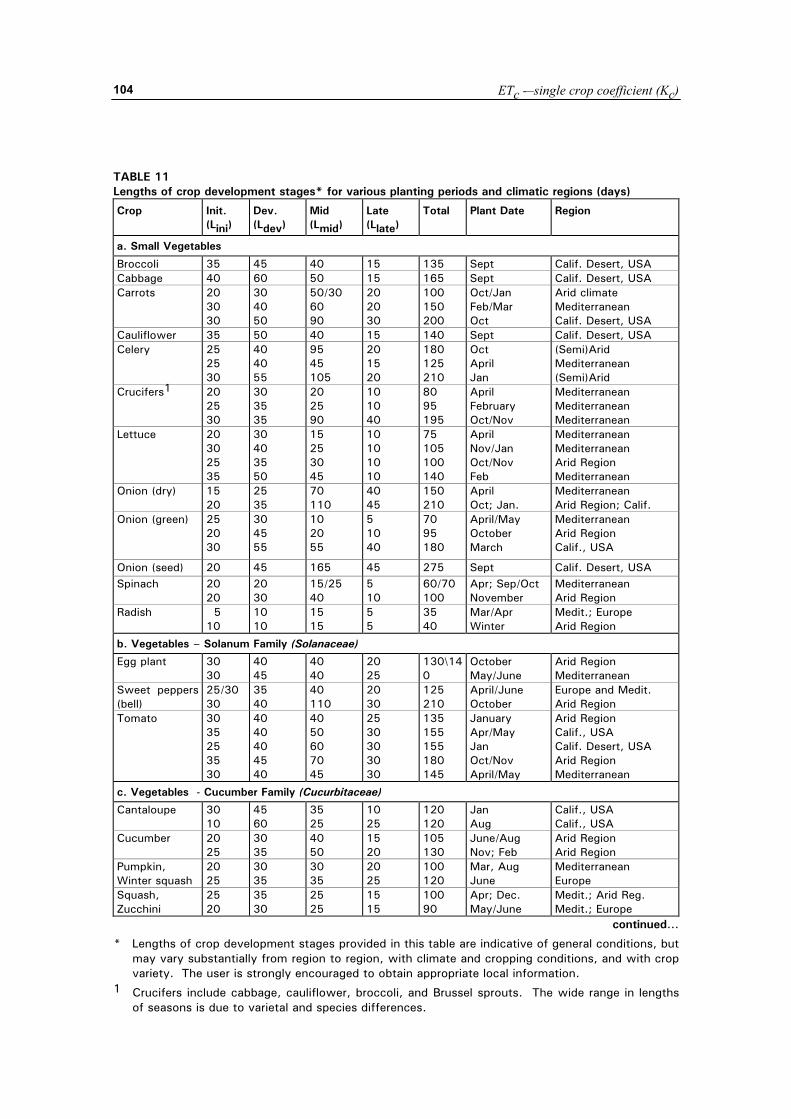
ETc -–single crop coefficient (Kc)
104
TABLE 11 Lengths of crop development stages* for various planting periods and climatic regions (days)
Crop Init. (Lini)
Dev. (Ldev)
Mid (Lmid)
Late (Llate)
Total Plant Date Region
a. Small Vegetables
Broccoli 35 45 40 15 135 Sept Calif. Desert, USA Cabbage 40 60 50 15 165 Sept Calif. Desert, USA Carrots 20
30 30
30 40 50
50/30 60 90
20 20 30
100 150 200
Oct/Jan Feb/Mar Oct
Arid climate Mediterranean Calif. Desert, USA
Cauliflower 35 50 40 15 140 Sept Calif. Desert, USA Celery 25
25 30
40 40 55
95 45 105
20 15 20
180 125 210
Oct April Jan
(Semi)Arid Mediterranean (Semi)Arid
Crucifers1 20 25 30
30 35 35
20 25 90
10 10 40
80 95 195
April February Oct/Nov
Mediterranean Mediterranean Mediterranean
Lettuce 20 30 25 35
30 40 35 50
15 25 30 45
10 10 10 10
75 105 100 140
April Nov/Jan Oct/Nov Feb
Mediterranean Mediterranean Arid Region Mediterranean
Onion (dry) 15 20
25 35
70 110
40 45
150 210
April Oct; Jan.
Mediterranean Arid Region; Calif.
Onion (green) 25 20 30
30 45 55
10 20 55
5 10 40
70 95 180
April/May October March
Mediterranean Arid Region Calif., USA
Onion (seed) 20 45 165 45 275 Sept Calif. Desert, USA Spinach 20
20 20 30
15/25 40
5 10
60/70 100
Apr; Sep/Oct November
Mediterranean Arid Region
Radish 5 10
10 10
15 15
5 5
35 40
Mar/Apr Winter
Medit.; Europe Arid Region
b. Vegetables – Solanum Family (Solanaceae)
Egg plant 30 30
40 45
40 40
20 25
130\140
October May/June
Arid Region Mediterranean
Sweet peppers (bell)
25/30 30
35 40
40 110
20 30
125 210
April/June October
Europe and Medit. Arid Region
Tomato 30 35 25 35 30
40 40 40 45 40
40 50 60 70 45
25 30 30 30 30
135 155 155 180 145
January Apr/May Jan Oct/Nov April/May
Arid Region Calif., USA Calif. Desert, USA Arid Region Mediterranean
c. Vegetables - Cucumber Family (Cucurbitaceae)
Cantaloupe 30 10
45 60
35 25
10 25
120 120
Jan Aug
Calif., USA Calif., USA
Cucumber 20 25
30 35
40 50
15 20
105 130
June/Aug Nov; Feb
Arid Region Arid Region
Pumpkin, Winter squash
20 25
30 35
30 35
20 25
100 120
Mar, Aug June
Mediterranean Europe
Squash, Zucchini
25 20
35 30
25 25
15 15
100 90
Apr; Dec. May/June
Medit.; Arid Reg. Medit.; Europe
continued…
* Lengths of crop development stages provided in this table are indicative of general conditions, but may vary substantially from region to region, with climate and cropping conditions, and with crop variety. The user is strongly encouraged to obtain appropriate local information.
1 Crucifers include cabbage, cauliflower, broccoli, and Brussel sprouts. The wide range in lengths of seasons is due to varietal and species differences.
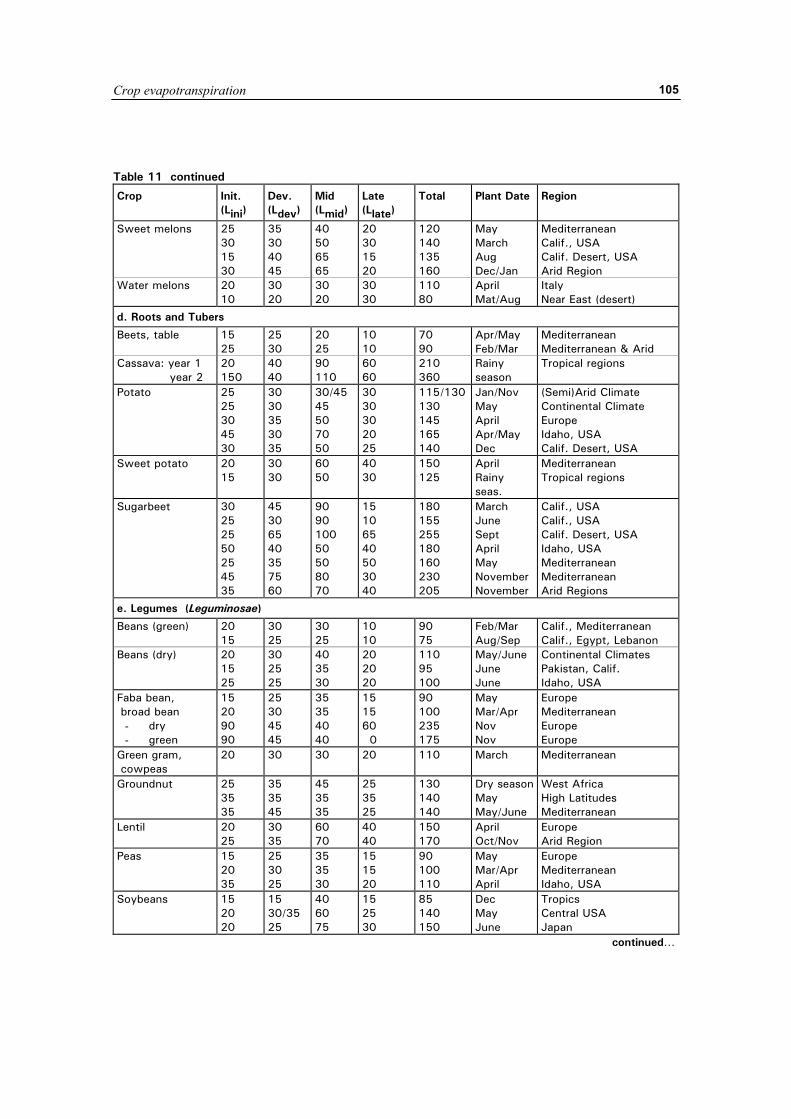
Crop evapotranspiration
105
Table 11 continued
Crop Init. (Lini)
Dev. (Ldev)
Mid (Lmid)
Late (Llate)
Total Plant Date Region
Sweet melons 25 30 15 30
35 30 40 45
40 50 65 65
20 30 15 20
120 140 135 160
May March Aug Dec/Jan
Mediterranean Calif., USA Calif. Desert, USA Arid Region
Water melons 20 10
30 20
30 20
30 30
110 80
April Mat/Aug
Italy Near East (desert)
d. Roots and Tubers
Beets, table 15 25
25 30
20 25
10 10
70 90
Apr/May Feb/Mar
Mediterranean Mediterranean & Arid
Cassava: year 1 year 2
20 150
40 40
90 110
60 60
210 360
Rainy season
Tropical regions
Potato 25 25 30 45 30
30 30 35 30 35
30/45 45 50 70 50
30 30 30 20 25
115/130130 145 165 140
Jan/Nov May April Apr/May Dec
(Semi)Arid Climate Continental Climate Europe Idaho, USA Calif. Desert, USA
Sweet potato 20 15
30 30
60 50
40 30
150 125
April Rainy seas.
Mediterranean Tropical regions
Sugarbeet 30 25 25 50 25 45 35
45 30 65 40 35 75 60
90 90 100 50 50 80 70
15 10 65 40 50 30 40
180 155 255 180 160 230 205
March June Sept April May November November
Calif., USA Calif., USA Calif. Desert, USA Idaho, USA Mediterranean Mediterranean Arid Regions
e. Legumes (Leguminosae)
Beans (green) 20 15
30 25
30 25
10 10
90 75
Feb/Mar Aug/Sep
Calif., Mediterranean Calif., Egypt, Lebanon
Beans (dry) 20 15 25
30 25 25
40 35 30
20 20 20
110 95 100
May/June June June
Continental Climates Pakistan, Calif. Idaho, USA
Faba bean, broad bean
- dry - green
15 20 90 90
25 30 45 45
35 35 40 40
15 15 60 0
90 100 235 175
May Mar/Apr Nov Nov
Europe Mediterranean Europe Europe
Green gram, cowpeas
20 30 30 20 110 March Mediterranean
Groundnut 25 35 35
35 35 45
45 35 35
25 35 25
130 140 140
Dry seasonMay May/June
West Africa High Latitudes Mediterranean
Lentil 20 25
30 35
60 70
40 40
150 170
April Oct/Nov
Europe Arid Region
Peas 15 20 35
25 30 25
35 35 30
15 15 20
90 100 110
May Mar/Apr April
Europe Mediterranean Idaho, USA
Soybeans 15 20 20
15 30/35 25
40 60 75
15 25 30
85 140 150
Dec May June
Tropics Central USA Japan
continued…
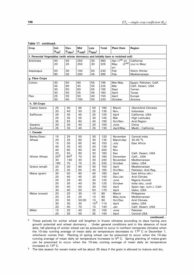
ETc -–single crop coefficient (Kc)
106
Table 11 continued.
Crop Init. (Lini)
Dev. (Ldev)
Mid (Lmid)
Late (Llate)
Total Plant Date Region
f. Perennial Vegetables (with winter dormancy and initially bare or mulched soil)
Artichoke 40 20
40 25
250 250
30 30
360 325
Apr (1st yr) May (2nd
yr)
California (cut in May)
Asparagus 50 90
30 30
100 200
50 45
230 365
Feb Feb
Warm Winter Mediterranean
g. Fibre Crops
Cotton 30 45 30 30
50 90 50 50
60 45 60 55
55 45 55 45
195 225 195 180
Mar-May Mar Sept April
Egypt; Pakistan; Calif. Calif. Desert, USA Yemen Texas
Flax 25 30
35 40
50 100
40 50
150 220
April October
Europe Arizona
h. Oil Crops
Castor beans 25 20
40 40
65 50
50 25
180 135
March Nov.
(Semi)Arid Climates Indonesia
Safflower 20 25 35
35 35 55
45 55 60
25 30 40
125 145 190
April Mar Oct/Nov
California, USA High Latitudes Arid Region
Sesame 20 30 40 20 100 June China Sunflower 25 35 45 25 130 April/May Medit.; California i. Cereals
Barley/Oats/ Wheat
15 20 15 40 40 20
25 25 30 30 60 50
50 60 65 40 60 60
30 30 40 20 40 30
120 135 150 130 200 160
November March/Apr July Apr Nov Dec
Central India 35-45 oL East Africa Calif. Desert, USA
Winter Wheat 202 30 160
602 140 75
70 40 75
30 30 25
180 240 335
December November October
Calif., USA Mediterranean Idaho, USA
Grains (small) 20 25
30 35
60 65
40 40
150 165
April Oct/Nov
Mediterranean Pakistan; Arid Reg.
Maize (grain) 30 25 20 20 30 30
50 40 35 35 40 40
60 45 40 40 50 50
40 30 30 30 30 50
180 140 125 125 150 170
April Dec/Jan June October April April
East Africa (alt.) Arid Climate Nigeria (humid) India (dry, cool) Spain (spr, sum.); Calif. Idaho, USA
Maize (sweet) 20 20 20 30 20
20 25 30 30 40
30 25 50/30 30 70
10 10 10 103 10
80 80 90 110 140
March May/June Oct/Dec April Jan
Philippines Mediterranean Arid Climate Idaho, USA Calif. Desert, USA
Millet 15 20
25 30
40 55
25 35
105 140
June April
Pakistan Central USA
continued… 2 These periods for winter wheat will lengthen in frozen climates according to days having zero
growth potential and wheat dormancy . Under general conditions and in the absence of local data, fall planting of winter wheat can be presumed to occur in northern temperate climates when the 10-day running average of mean daily air temperature decreases to 17o C or December 1, whichever comes first. Planting of spring wheat can be presumed to occur when the 10-day running average of mean daily air temperature increases to 5o C. Spring planting of maize-grain can be presumed to occur when the 10-day running average of mean daily air temperature increases to 13o C.
3 The late season for sweet maize will be about 35 days if the grain is allowed to mature and dry.
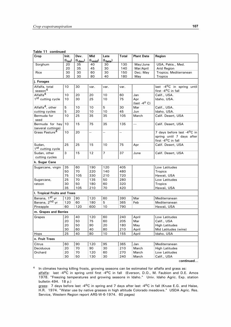
Crop evapotranspiration
107
Table 11 continued Crop Init.
(Lini) Dev. (Ldev)
Mid (Lmid)
Late (Llate)
Total Plant Date Region
Sorghum 20 20
35 35
40 45
30 30
130 140
May/June Mar/April
USA, Pakis., Med. Arid Region
Rice 30 30
30 30
60 80
30 40
150 180
Dec; May May
Tropics; Mediterranean Tropics
j. Forages
Alfalfa, total season4
10 30 var. var. var. last -4oC in spring until first -4oC in fall
Alfalfa4 1st cutting cycle
10 10
20 30
20 25
10 10
60 75
Jan Apr (last -4o C)
Calif., USA. Idaho, USA.
Alfalfa4, other cutting cycles
5 5
10 20
10 10
5 10
30 45
Mar Jun
Calif., USA. Idaho, USA.
Bermuda for seed
10 25 35 35 105 March Calif. Desert, USA
Bermuda for hay (several cuttings)
10 15 75 35 135 --- Calif. Desert, USA
Grass Pasture4 10 20 -- -- -- 7 days before last -4oC in spring until 7 days after first -4oC in fall
Sudan, 1st cutting cycle
25 25 15 10 75 Apr Calif. Desert, USA
Sudan, other cutting cycles
3 15 12 7 37 June Calif. Desert, USA
k. Sugar Cane
Sugarcane, virgin 35 50 75
60 70 105
190 220 330
120 140 210
405 480 720
Low Latitudes Tropics Hawaii, USA
Sugarcane, ratoon
25 30 35
70 50 105
135 180 210
50 60 70
280 320 420
Low Latitudes Tropics Hawaii, USA
l. Tropical Fruits and Trees
Banana, 1st yr 120 90 120 60 390 Mar Mediterranean Banana, 2nd yr 120 60 180 5 365 Feb Mediterranean Pineapple 60 120 600 10 790 Hawaii, USA
m. Grapes and Berries
Grapes 20 20 20 30
40 50 50 60
120 75 90 40
60 60 20 80
240 205 180 210
April Mar May April
Low Latitudes Calif., USA High Latitudes Mid Latitudes (wine)
Hops 25 40 80 10 155 April Idaho, USA
n. Fruit Trees
Citrus 60 90 120 95 365 Jan Mediterranean Deciduous Orchard
20 20 30
70 70 50
90 120 130
30 60 30
210 270 240
March March March
High Latitudes Low Latitudes Calif., USA
continued…
4 In climates having killing frosts, growing seasons can be estimated for alfalfa and grass as: alfalfa: last -4oC in spring until first -4oC in fall (Everson, D.O., M. Faubion and D.E. Amos
1978. "Freezing temperatures and growing seasons in Idaho." Univ. Idaho Agric. Exp. station bulletin 494. 18 p.)
grass: 7 days before last -4oC in spring and 7 days after last -4oC in fall (Kruse E.G. and Haise, H.R. 1974. "Water use by native grasses in high altitude Colorado meadows." USDA Agric. Res. Service, Western Region report ARS-W-6-1974. 60 pages)
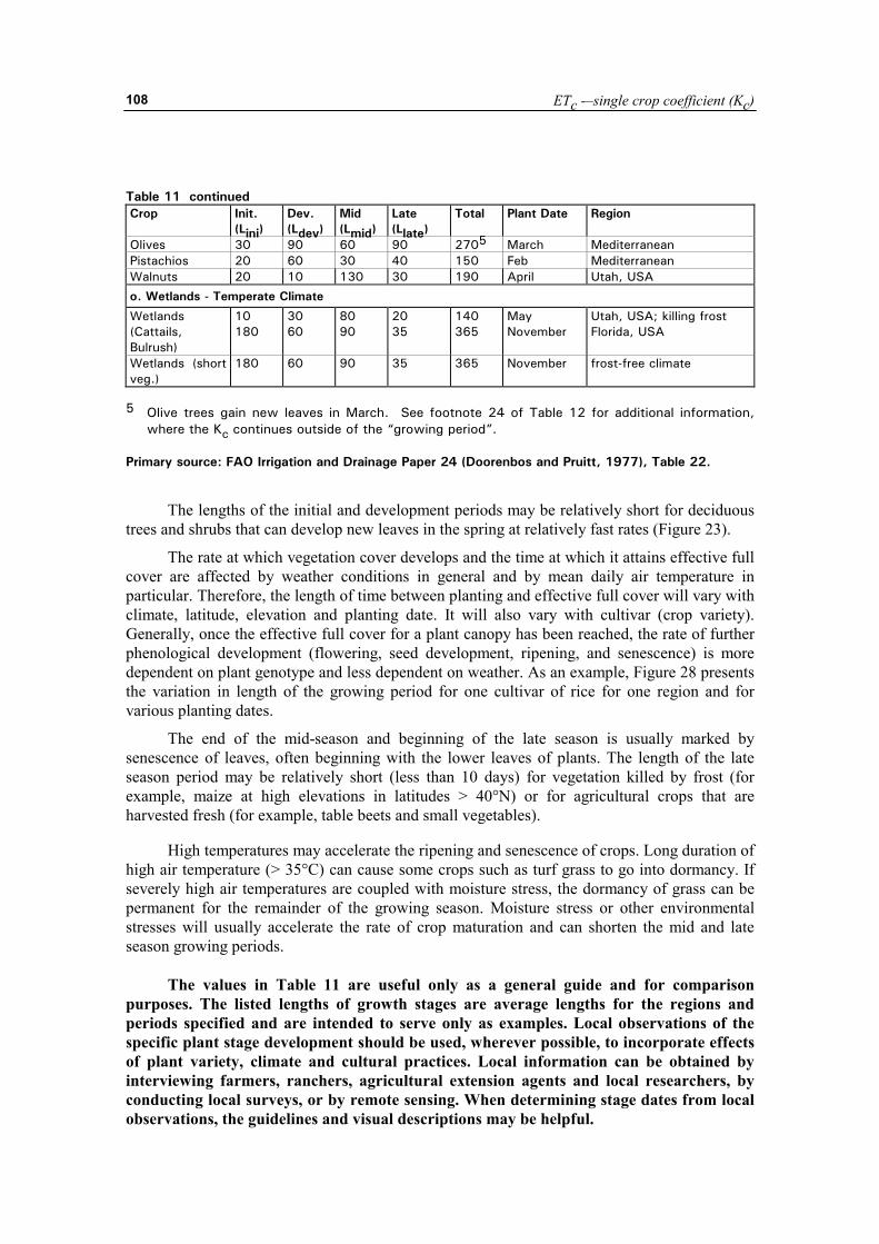
ETc -–single crop coefficient (Kc)
108
Table 11 continued Crop Init.
(Lini) Dev. (Ldev)
Mid (Lmid)
Late (Llate)
Total Plant Date Region
Olives 30 90 60 90 2705 March Mediterranean Pistachios 20 60 30 40 150 Feb Mediterranean Walnuts 20 10 130 30 190 April Utah, USA
o. Wetlands - Temperate Climate
Wetlands (Cattails, Bulrush)
10 180
30 60
80 90
20 35
140 365
May November
Utah, USA; killing frost Florida, USA
Wetlands (short veg.)
180 60 90 35 365 November frost-free climate
5 Olive trees gain new leaves in March. See footnote 24 of Table 12 for additional information,
where the Kc continues outside of the “growing period”. Primary source: FAO Irrigation and Drainage Paper 24 (Doorenbos and Pruitt, 1977), Table 22.
The lengths of the initial and development periods may be relatively short for deciduous trees and shrubs that can develop new leaves in the spring at relatively fast rates (Figure 23).
The rate at which vegetation cover develops and the time at which it attains effective full cover are affected by weather conditions in general and by mean daily air temperature in particular. Therefore, the length of time between planting and effective full cover will vary with climate, latitude, elevation and planting date. It will also vary with cultivar (crop variety). Generally, once the effective full cover for a plant canopy has been reached, the rate of further phenological development (flowering, seed development, ripening, and senescence) is more dependent on plant genotype and less dependent on weather. As an example, Figure 28 presents the variation in length of the growing period for one cultivar of rice for one region and for various planting dates.
The end of the mid-season and beginning of the late season is usually marked by senescence of leaves, often beginning with the lower leaves of plants. The length of the late season period may be relatively short (less than 10 days) for vegetation killed by frost (for example, maize at high elevations in latitudes > 40°N) or for agricultural crops that are harvested fresh (for example, table beets and small vegetables). High temperatures may accelerate the ripening and senescence of crops. Long duration of high air temperature (> 35°C) can cause some crops such as turf grass to go into dormancy. If severely high air temperatures are coupled with moisture stress, the dormancy of grass can be permanent for the remainder of the growing season. Moisture stress or other environmental stresses will usually accelerate the rate of crop maturation and can shorten the mid and late season growing periods.
The values in Table 11 are useful only as a general guide and for comparison purposes. The listed lengths of growth stages are average lengths for the regions and periods specified and are intended to serve only as examples. Local observations of the specific plant stage development should be used, wherever possible, to incorporate effects of plant variety, climate and cultural practices. Local information can be obtained by interviewing farmers, ranchers, agricultural extension agents and local researchers, by conducting local surveys, or by remote sensing. When determining stage dates from local observations, the guidelines and visual descriptions may be helpful.
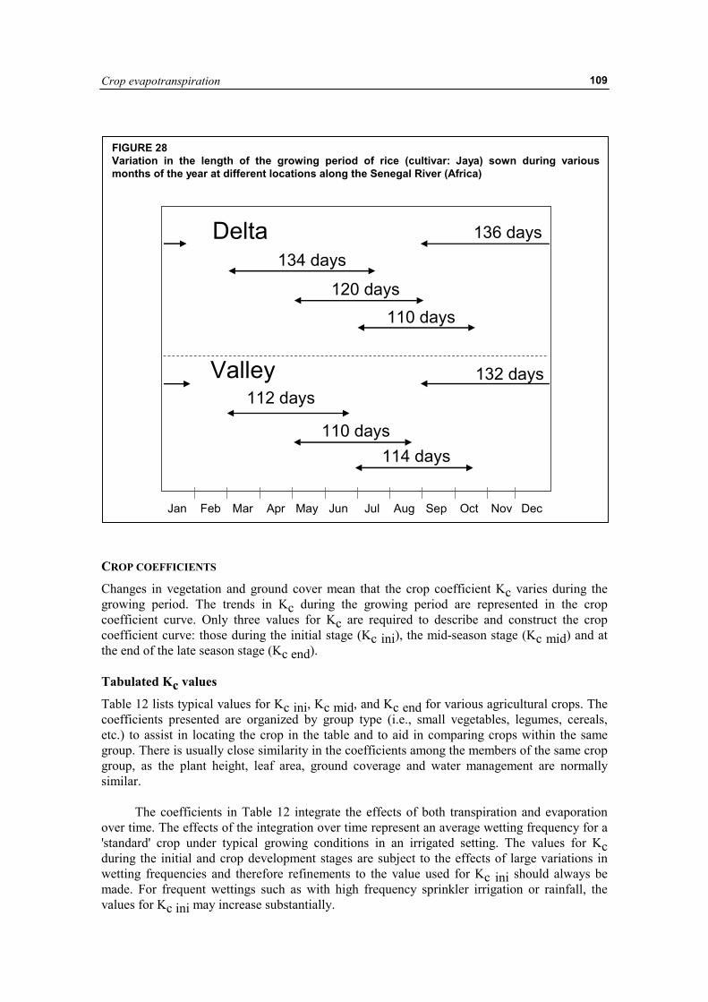
Crop evapotranspiration
109
CROP COEFFICIENTS
Changes in vegetation and ground cover mean that the crop coefficient Kc varies during the growing period. The trends in Kc during the growing period are represented in the crop coefficient curve. Only three values for Kc are required to describe and construct the crop coefficient curve: those during the initial stage (Kc ini), the mid-season stage (Kc mid) and at the end of the late season stage (Kc end). Tabulated Kc values
Table 12 lists typical values for Kc ini, Kc mid, and Kc end for various agricultural crops. The coefficients presented are organized by group type (i.e., small vegetables, legumes, cereals, etc.) to assist in locating the crop in the table and to aid in comparing crops within the same group. There is usually close similarity in the coefficients among the members of the same crop group, as the plant height, leaf area, ground coverage and water management are normally similar.
The coefficients in Table 12 integrate the effects of both transpiration and evaporation over time. The effects of the integration over time represent an average wetting frequency for a 'standard' crop under typical growing conditions in an irrigated setting. The values for Kc during the initial and crop development stages are subject to the effects of large variations in wetting frequencies and therefore refinements to the value used for Kc ini should always be made. For frequent wettings such as with high frequency sprinkler irrigation or rainfall, the values for Kc ini may increase substantially.
FIGURE 28 Variation in the length of the growing period of rice (cultivar: Jaya) sown during various months of the year at different locations along the Senegal River (Africa)
Jan Feb Mar Apr May Jun Jul Aug Sep Oct Nov Dec
136 days134 days
110 days
110 days
120 days
Delta
Valley 132 days112 days
114 days
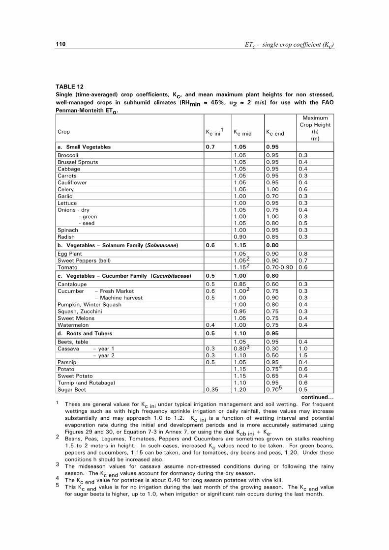
ETc -–single crop coefficient (Kc)
110
TABLE 12 Single (time-averaged) crop coefficients, Kc, and mean maximum plant heights for non stressed, well-managed crops in subhumid climates (RHmin ≈≈≈≈ 45%, u2 ≈≈≈≈ 2 m/s) for use with the FAO Penman-Monteith ETo. Crop
Kc ini
1
Kc mid
Kc end
Maximum Crop Height
(h) (m)
a. Small Vegetables 0.7 1.05 0.95
Broccoli 1.05 0.95 0.3 Brussel Sprouts 1.05 0.95 0.4 Cabbage 1.05 0.95 0.4 Carrots 1.05 0.95 0.3 Cauliflower 1.05 0.95 0.4 Celery 1.05 1.00 0.6 Garlic 1.00 0.70 0.3 Lettuce 1.00 0.95 0.3 Onions - dry 1.05 0.75 0.4
- green 1.00 1.00 0.3 - seed 1.05 0.80 0.5
Spinach 1.00 0.95 0.3 Radish 0.90 0.85 0.3
b. Vegetables – Solanum Family (Solanaceae) 0.6 1.15 0.80
Egg Plant 1.05 0.90 0.8 Sweet Peppers (bell) 1.052 0.90 0.7 Tomato 1.152 0.70-0.90 0.6
c. Vegetables – Cucumber Family (Cucurbitaceae) 0.5 1.00 0.80
Cantaloupe 0.5 0.85 0.60 0.3 Cucumber – Fresh Market 0.6 1.002 0.75 0.3 – Machine harvest 0.5 1.00 0.90 0.3 Pumpkin, Winter Squash 1.00 0.80 0.4 Squash, Zucchini 0.95 0.75 0.3 Sweet Melons 1.05 0.75 0.4 Watermelon 0.4 1.00 0.75 0.4 d. Roots and Tubers 0.5 1.10 0.95
Beets, table 1.05 0.95 0.4 Cassava – year 1 0.3 0.803 0.30 1.0 – year 2 0.3 1.10 0.50 1.5 Parsnip 0.5 1.05 0.95 0.4 Potato 1.15 0.754 0.6 Sweet Potato 1.15 0.65 0.4 Turnip (and Rutabaga) 1.10 0.95 0.6 Sugar Beet 0.35 1.20 0.705 0.5
continued…
1 These are general values for Kc ini under typical irrigation management and soil wetting. For frequent wettings such as with high frequency sprinkle irrigation or daily rainfall, these values may increase substantially and may approach 1.0 to 1.2. Kc ini is a function of wetting interval and potential evaporation rate during the initial and development periods and is more accurately estimated using Figures 29 and 30, or Equation 7-3 in Annex 7, or using the dual Kcb ini + Ke.
2 Beans, Peas, Legumes, Tomatoes, Peppers and Cucumbers are sometimes grown on stalks reaching 1.5 to 2 meters in height. In such cases, increased Kc values need to be taken. For green beans, peppers and cucumbers, 1.15 can be taken, and for tomatoes, dry beans and peas, 1.20. Under these conditions h should be increased also.
3 The midseason values for cassava assume non-stressed conditions during or following the rainy season. The Kc end values account for dormancy during the dry season.
4 The Kc end value for potatoes is about 0.40 for long season potatoes with vine kill. 5 This Kc end value is for no irrigation during the last month of the growing season. The Kc end value
for sugar beets is higher, up to 1.0, when irrigation or significant rain occurs during the last month.
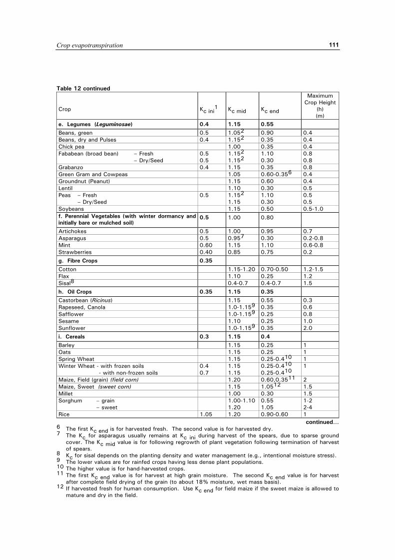
Crop evapotranspiration
111
Table 12 continued Crop
Kc ini
1
Kc mid
Kc end
Maximum Crop Height
(h) (m)
e. Legumes (Leguminosae) 0.4 1.15 0.55
Beans, green 0.5 1.052 0.90 0.4 Beans, dry and Pulses 0.4 1.152 0.35 0.4 Chick pea 1.00 0.35 0.4 Fababean (broad bean) – Fresh 0.5 1.152 1.10 0.8 – Dry/Seed 0.5 1.152 0.30 0.8 Grabanzo 0.4 1.15 0.35 0.8 Green Gram and Cowpeas 1.05 0.60-0.356 0.4 Groundnut (Peanut) 1.15 0.60 0.4 Lentil 1.10 0.30 0.5 Peas – Fresh 0.5 1.152 1.10 0.5 – Dry/Seed 1.15 0.30 0.5 Soybeans 1.15 0.50 0.5-1.0 f. Perennial Vegetables (with winter dormancy and initially bare or mulched soil)
0.5 1.00 0.80
Artichokes 0.5 1.00 0.95 0.7 Asparagus 0.5 0.957 0.30 0.2-0.8 Mint 0.60 1.15 1.10 0.6-0.8 Strawberries 0.40 0.85 0.75 0.2 g. Fibre Crops 0.35 Cotton 1.15-1.20 0.70-0.50 1.2-1.5 Flax 1.10 0.25 1.2 Sisal8 0.4-0.7 0.4-0.7 1.5 h. Oil Crops 0.35 1.15 0.35
Castorbean (Ricinus) 1.15 0.55 0.3 Rapeseed, Canola 1.0-1.159 0.35 0.6 Safflower 1.0-1.159 0.25 0.8 Sesame 1.10 0.25 1.0 Sunflower 1.0-1.159 0.35 2.0 i. Cereals 0.3 1.15 0.4
Barley 1.15 0.25 1 Oats 1.15 0.25 1 Spring Wheat 1.15 0.25-0.410 1 Winter Wheat - with frozen soils
- with non-frozen soils 0.4 0.7
1.15 1.15
0.25-0.410
0.25-0.410 1
Maize, Field (grain) (field corn) 1.20 0.60,0.3511 2 Maize, Sweet (sweet corn) 1.15 1.0512 1.5 Millet 1.00 0.30 1.5 Sorghum – grain 1.00-1.10 0.55 1-2 – sweet 1.20 1.05 2-4 Rice 1.05 1.20 0.90-0.60 1
continued… 6 The first Kc end is for harvested fresh. The second value is for harvested dry. 7 The Kc for asparagus usually remains at Kc ini during harvest of the spears, due to sparse ground
cover. The Kc mid value is for following regrowth of plant vegetation following termination of harvest of spears.
8 Kc for sisal depends on the planting density and water management (e.g., intentional moisture stress). 9 The lower values are for rainfed crops having less dense plant populations. 10 The higher value is for hand-harvested crops. 11 The first Kc end value is for harvest at high grain moisture. The second Kc end value is for harvest
after complete field drying of the grain (to about 18% moisture, wet mass basis). 12 If harvested fresh for human consumption. Use Kc end for field maize if the sweet maize is allowed to
mature and dry in the field.
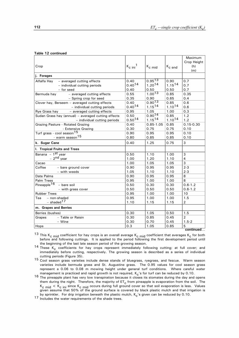
ETc -–single crop coefficient (Kc)
112
Table 12 continued Crop
Kc ini
1
Kc mid
Kc end
Maximum Crop Height
(h) (m)
j. Forages
Alfalfa Hay – averaged cutting effects 0.40 0.9513 0.90 0.7 – individual cutting periods 0.4014 1.2014 1.1514 0.7 – for seed 0.40 0.50 0.50 0.7 Bermuda hay – averaged cutting effects 0.55 1.0013 0.85 0.35 – Spring crop for seed 0.35 0.90 0.65 0.4 Clover hay, Berseem – averaged cutting effects 0.40 0.9013 0.85 0.6 – individual cutting periods 0.4014 1.1514 1.1014 0.6 Rye Grass hay – averaged cutting effects 0.95 1.05 1.00 0.3 Sudan Grass hay (annual) – averaged cutting effects 0.50 0.9014 0.85 1.2 – individual cutting periods 0.5014 1.1514 1.1014 1.2 Grazing Pasture - Rotated Grazing 0.40 0.85-1.05 0.85 0.15-0.30
- Extensive Grazing 0.30 0.75 0.75 0.10 Turf grass - cool season15 0.90 0.95 0.95 0.10
- warm season15 0.80 0.85 0.85 0.10
k. Sugar Cane 0.40 1.25 0.75 3
l. Tropical Fruits and Trees
Banana – 1st year 0.50 1.10 1.00 3 – 2nd year 1.00 1.20 1.10 4 Cacao 1.00 1.05 1.05 3 Coffee – bare ground cover 0.90 0.95 0.95 2-3 – with weeds 1.05 1.10 1.10 2-3 Date Palms 0.90 0.95 0.95 8 Palm Trees 0.95 1.00 1.00 8 Pineapple16 – bare soil 0.50 0.30 0.30 0.6-1.2 – with grass cover 0.50 0.50 0.50 0.6-1.2 Rubber Trees 0.95 1.00 1.00 10 Tea – non-shaded 0.95 1.00 1.00 1.5 – shaded17 1.10 1.15 1.15 2
m. Grapes and Berries
Berries (bushes) 0.30 1.05 0.50 1.5 Grapes – Table or Raisin 0.30 0.85 0.45 2 – Wine 0.30 0.70 0.45 1.5-2 Hops 0.3 1.05 0.85 5
continued… 13 This Kc mid coefficient for hay crops is an overall average Kc mid coefficient that averages Kc for both
before and following cuttings. It is applied to the period following the first development period until the beginning of the last late season period of the growing season.
14 These Kc coefficients for hay crops represent immediately following cutting; at full cover; and immediately before cutting, respectively. The growing season is described as a series of individual cutting periods (Figure 35).
15 Cool season grass varieties include dense stands of bluegrass, ryegrass, and fescue. Warm season varieties include bermuda grass and St. Augustine grass. The 0.95 values for cool season grass represent a 0.06 to 0.08 m mowing height under general turf conditions. Where careful water management is practiced and rapid growth is not required, Kc's for turf can be reduced by 0.10.
16 The pineapple plant has very low transpiration because it closes its stomates during the day and opens them during the night. Therefore, the majority of ETc from pineapple is evaporation from the soil. The Kc mid < Kc ini since Kc mid occurs during full ground cover so that soil evaporation is less. Values given assume that 50% of the ground surface is covered by black plastic mulch and that irrigation is by sprinkler. For drip irrigation beneath the plastic mulch, Kc's given can be reduced by 0.10.
17 Includes the water requirements of the shade trees.
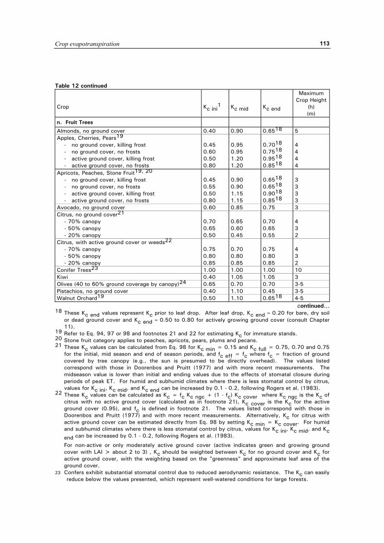
Crop evapotranspiration
113
Table 12 continued Crop
Kc ini
1
Kc mid
Kc end
Maximum Crop Height
(h) (m)
n. Fruit Trees
Almonds, no ground cover 0.40 0.90 0.6518 5 Apples, Cherries, Pears19 - no ground cover, killing frost 0.45 0.95 0.7018 4 - no ground cover, no frosts 0.60 0.95 0.7518 4 - active ground cover, killing frost 0.50 1.20 0.9518 4 - active ground cover, no frosts 0.80 1.20 0.8518 4 Apricots, Peaches, Stone Fruit19, 20 - no ground cover, killing frost 0.45 0.90 0.6518 3 - no ground cover, no frosts 0.55 0.90 0.6518 3 - active ground cover, killing frost 0.50 1.15 0.9018 3 - active ground cover, no frosts 0.80 1.15 0.8518 3 Avocado, no ground cover 0.60 0.85 0.75 3 Citrus, no ground cover21 - 70% canopy 0.70 0.65 0.70 4 - 50% canopy 0.65 0.60 0.65 3 - 20% canopy 0.50 0.45 0.55 2 Citrus, with active ground cover or weeds22 - 70% canopy 0.75 0.70 0.75 4 - 50% canopy 0.80 0.80 0.80 3 - 20% canopy 0.85 0.85 0.85 2 Conifer Trees23 1.00 1.00 1.00 10 Kiwi 0.40 1.05 1.05 3 Olives (40 to 60% ground coverage by canopy)24 0.65 0.70 0.70 3-5 Pistachios, no ground cover 0.40 1.10 0.45 3-5 Walnut Orchard19 0.50 1.10 0.6518 4-5 continued… 18 These Kc end values represent Kc prior to leaf drop. After leaf drop, Kc end ≈ 0.20 for bare, dry soil
or dead ground cover and Kc end ≈ 0.50 to 0.80 for actively growing ground cover (consult Chapter 11).
19 Refer to Eq. 94, 97 or 98 and footnotes 21 and 22 for estimating Kc for immature stands. 20 Stone fruit category applies to peaches, apricots, pears, plums and pecans. 21 These Kc values can be calculated from Eq. 98 for Kc min = 0.15 and Kc full = 0.75, 0.70 and 0.75
for the initial, mid season and end of season periods, and fc eff = fc where fc = fraction of ground covered by tree canopy (e.g., the sun is presumed to be directly overhead). The values listed correspond with those in Doorenbos and Pruitt (1977) and with more recent measurements. The midseason value is lower than initial and ending values due to the effects of stomatal closure during periods of peak ET. For humid and subhumid climates where there is less stomatal control by citrus, values for Kc ini, Kc mid, and Kc end can be increased by 0.1 - 0.2, following Rogers et al. (1983).
22 These Kc values can be calculated as Kc = fc Kc ngc + (1 - fc) Kc cover where Kc ngc is the Kc of citrus with no active ground cover (calculated as in footnote 21), Kc cover is the Kc for the active ground cover (0.95), and fc is defined in footnote 21. The values listed correspond with those in Doorenbos and Pruitt (1977) and with more recent measurements. Alternatively, Kc for citrus with active ground cover can be estimated directly from Eq. 98 by setting Kc min = Kc cover. For humid and subhumid climates where there is less stomatal control by citrus, values for Kc ini, Kc mid, and Kc end can be increased by 0.1 - 0.2, following Rogers et al. (1983).
For non-active or only moderately active ground cover (active indicates green and growing ground cover with LAI > about 2 to 3) , Kc should be weighted between Kc for no ground cover and Kc for active ground cover, with the weighting based on the "greenness" and approximate leaf area of the ground cover.
23 Confers exhibit substantial stomatal control due to reduced aerodynamic resistance. The Kc can easily reduce below the values presented, which represent well-watered conditions for large forests.
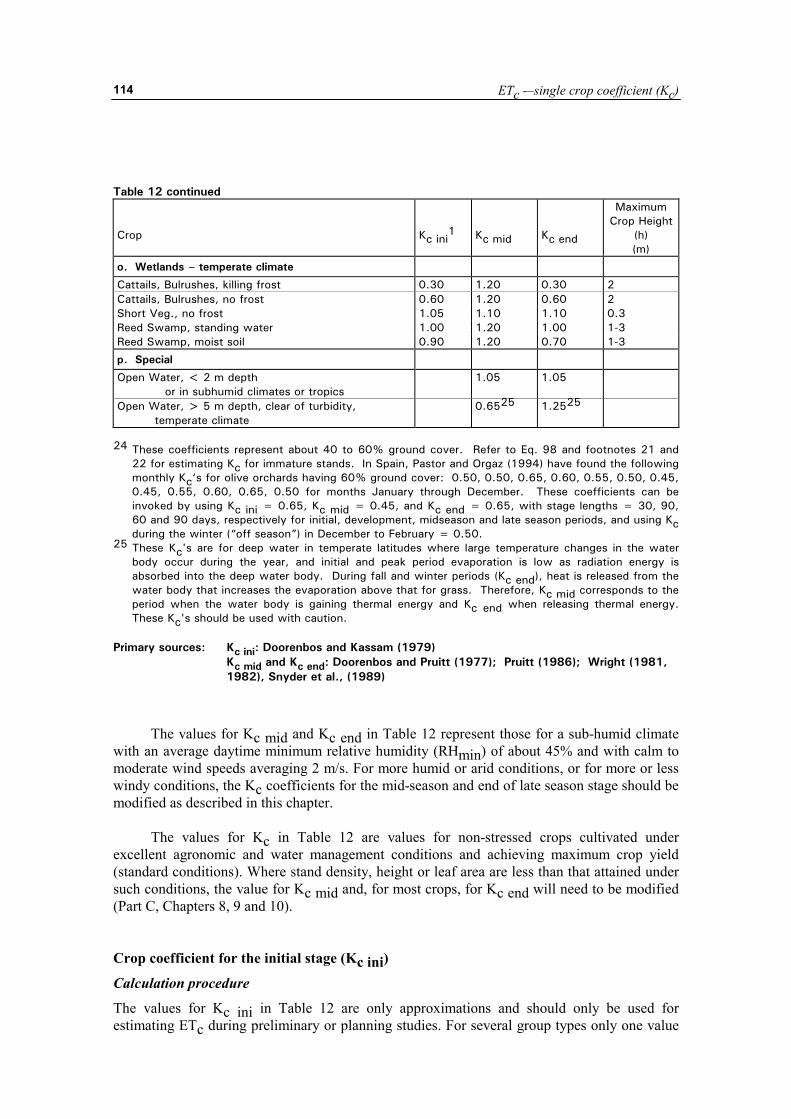
ETc -–single crop coefficient (Kc)
114
Table 12 continued Crop
Kc ini
1
Kc mid
Kc end
Maximum Crop Height
(h) (m)
o. Wetlands – temperate climate
Cattails, Bulrushes, killing frost 0.30 1.20 0.30 2 Cattails, Bulrushes, no frost 0.60 1.20 0.60 2 Short Veg., no frost 1.05 1.10 1.10 0.3 Reed Swamp, standing water 1.00 1.20 1.00 1-3 Reed Swamp, moist soil 0.90 1.20 0.70 1-3
p. Special
Open Water, < 2 m depth or in subhumid climates or tropics
1.05 1.05
Open Water, > 5 m depth, clear of turbidity, temperate climate
0.6525 1.2525
24 These coefficients represent about 40 to 60% ground cover. Refer to Eq. 98 and footnotes 21 and
22 for estimating Kc for immature stands. In Spain, Pastor and Orgaz (1994) have found the following monthly Kc‘s for olive orchards having 60% ground cover: 0.50, 0.50, 0.65, 0.60, 0.55, 0.50, 0.45, 0.45, 0.55, 0.60, 0.65, 0.50 for months January through December. These coefficients can be invoked by using Kc ini = 0.65, Kc mid = 0.45, and Kc end = 0.65, with stage lengths = 30, 90, 60 and 90 days, respectively for initial, development, midseason and late season periods, and using Kc during the winter (“off season”) in December to February = 0.50.
25 These Kc's are for deep water in temperate latitudes where large temperature changes in the water body occur during the year, and initial and peak period evaporation is low as radiation energy is absorbed into the deep water body. During fall and winter periods (Kc end), heat is released from the water body that increases the evaporation above that for grass. Therefore, Kc mid corresponds to the period when the water body is gaining thermal energy and Kc end when releasing thermal energy. These Kc's should be used with caution.
Primary sources: Kc ini: Doorenbos and Kassam (1979)
Kc mid and Kc end: Doorenbos and Pruitt (1977); Pruitt (1986); Wright (1981, 1982), Snyder et al., (1989)
The values for Kc mid and Kc end in Table 12 represent those for a sub-humid climate with an average daytime minimum relative humidity (RHmin) of about 45% and with calm to moderate wind speeds averaging 2 m/s. For more humid or arid conditions, or for more or less windy conditions, the Kc coefficients for the mid-season and end of late season stage should be modified as described in this chapter.
The values for Kc in Table 12 are values for non-stressed crops cultivated under excellent agronomic and water management conditions and achieving maximum crop yield (standard conditions). Where stand density, height or leaf area are less than that attained under such conditions, the value for Kc mid and, for most crops, for Kc end will need to be modified (Part C, Chapters 8, 9 and 10). Crop coefficient for the initial stage (Kc ini)
Calculation procedure
The values for Kc ini in Table 12 are only approximations and should only be used for estimating ETc during preliminary or planning studies. For several group types only one value
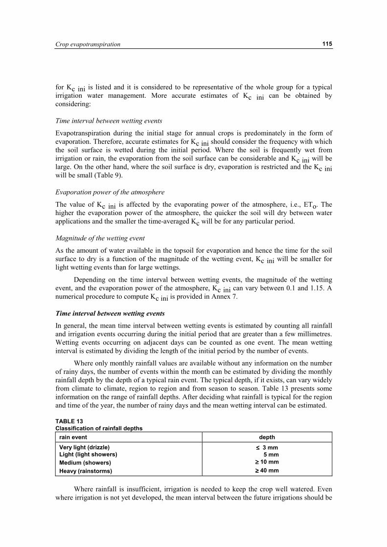
Crop evapotranspiration
115
for Kc ini is listed and it is considered to be representative of the whole group for a typical irrigation water management. More accurate estimates of Kc ini can be obtained by considering: Time interval between wetting events
Evapotranspiration during the initial stage for annual crops is predominately in the form of evaporation. Therefore, accurate estimates for Kc ini should consider the frequency with which the soil surface is wetted during the initial period. Where the soil is frequently wet from irrigation or rain, the evaporation from the soil surface can be considerable and Kc ini will be large. On the other hand, where the soil surface is dry, evaporation is restricted and the Kc ini will be small (Table 9). Evaporation power of the atmosphere
The value of Kc ini is affected by the evaporating power of the atmosphere, i.e., ETo. The higher the evaporation power of the atmosphere, the quicker the soil will dry between water applications and the smaller the time-averaged Kc will be for any particular period. Magnitude of the wetting event
As the amount of water available in the topsoil for evaporation and hence the time for the soil surface to dry is a function of the magnitude of the wetting event, Kc ini will be smaller for light wetting events than for large wettings.
Depending on the time interval between wetting events, the magnitude of the wetting event, and the evaporation power of the atmosphere, Kc ini can vary between 0.1 and 1.15. A numerical procedure to compute Kc ini is provided in Annex 7. Time interval between wetting events
In general, the mean time interval between wetting events is estimated by counting all rainfall and irrigation events occurring during the initial period that are greater than a few millimetres. Wetting events occurring on adjacent days can be counted as one event. The mean wetting interval is estimated by dividing the length of the initial period by the number of events.
Where only monthly rainfall values are available without any information on the number of rainy days, the number of events within the month can be estimated by dividing the monthly rainfall depth by the depth of a typical rain event. The typical depth, if it exists, can vary widely from climate to climate, region to region and from season to season. Table 13 presents some information on the range of rainfall depths. After deciding what rainfall is typical for the region and time of the year, the number of rainy days and the mean wetting interval can be estimated. TABLE 13 Classification of rainfall depths
rain event depth Very light (drizzle) Light (light showers) Medium (showers) Heavy (rainstorms)
≤≤≤≤ 3 mm 5 mm ≥≥≥≥ 10 mm ≥≥≥≥ 40 mm
Where rainfall is insufficient, irrigation is needed to keep the crop well watered. Even
where irrigation is not yet developed, the mean interval between the future irrigations should be
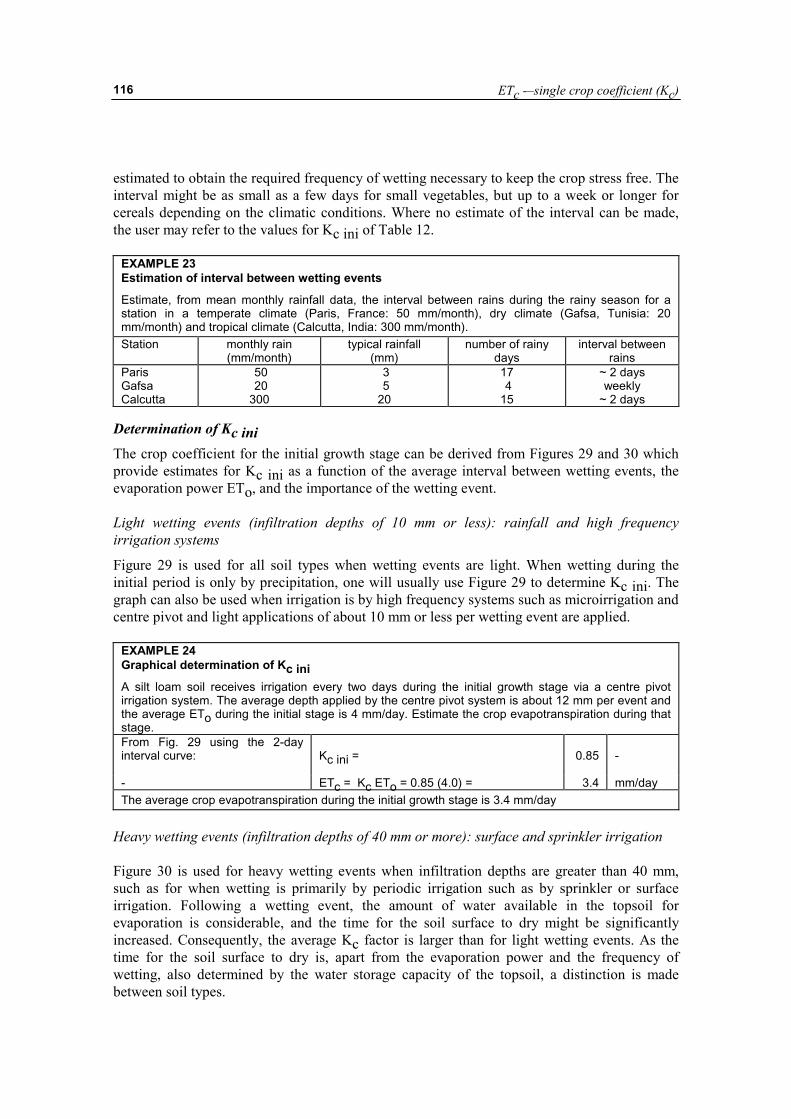
ETc -–single crop coefficient (Kc)
116
estimated to obtain the required frequency of wetting necessary to keep the crop stress free. The interval might be as small as a few days for small vegetables, but up to a week or longer for cereals depending on the climatic conditions. Where no estimate of the interval can be made, the user may refer to the values for Kc ini of Table 12.
EXAMPLE 23 Estimation of interval between wetting events
Estimate, from mean monthly rainfall data, the interval between rains during the rainy season for a station in a temperate climate (Paris, France: 50 mm/month), dry climate (Gafsa, Tunisia: 20 mm/month) and tropical climate (Calcutta, India: 300 mm/month). Station monthly rain
(mm/month) typical rainfall
(mm) number of rainy
days interval between
rains Paris Gafsa Calcutta
50 20 300
3 5 20
17 4 15
~ 2 days weekly
~ 2 days Determination of Kc ini
The crop coefficient for the initial growth stage can be derived from Figures 29 and 30 which provide estimates for Kc ini as a function of the average interval between wetting events, the evaporation power ETo, and the importance of the wetting event. Light wetting events (infiltration depths of 10 mm or less): rainfall and high frequency irrigation systems
Figure 29 is used for all soil types when wetting events are light. When wetting during the initial period is only by precipitation, one will usually use Figure 29 to determine Kc ini. The graph can also be used when irrigation is by high frequency systems such as microirrigation and centre pivot and light applications of about 10 mm or less per wetting event are applied.
EXAMPLE 24 Graphical determination of Kc ini
A silt loam soil receives irrigation every two days during the initial growth stage via a centre pivot irrigation system. The average depth applied by the centre pivot system is about 12 mm per event and the average ETo during the initial stage is 4 mm/day. Estimate the crop evapotranspiration during that stage. From Fig. 29 using the 2-day interval curve:
Kc ini =
0.85
-
- ETc = Kc ETo = 0.85 (4.0) = 3.4 mm/day The average crop evapotranspiration during the initial growth stage is 3.4 mm/day
Heavy wetting events (infiltration depths of 40 mm or more): surface and sprinkler irrigation Figure 30 is used for heavy wetting events when infiltration depths are greater than 40 mm, such as for when wetting is primarily by periodic irrigation such as by sprinkler or surface irrigation. Following a wetting event, the amount of water available in the topsoil for evaporation is considerable, and the time for the soil surface to dry might be significantly increased. Consequently, the average Kc factor is larger than for light wetting events. As the time for the soil surface to dry is, apart from the evaporation power and the frequency of wetting, also determined by the water storage capacity of the topsoil, a distinction is made between soil types.
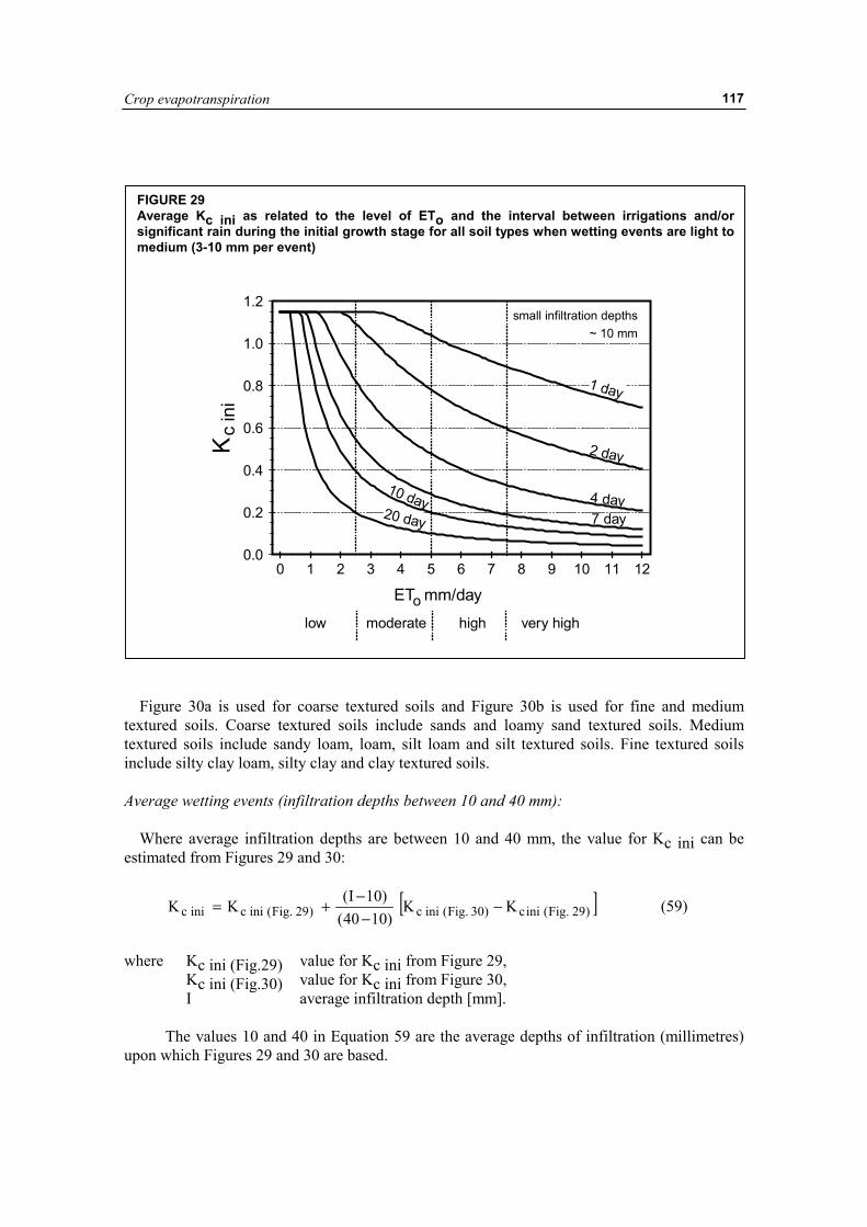
Crop evapotranspiration
117
Figure 30a is used for coarse textured soils and Figure 30b is used for fine and medium textured soils. Coarse textured soils include sands and loamy sand textured soils. Medium textured soils include sandy loam, loam, silt loam and silt textured soils. Fine textured soils include silty clay loam, silty clay and clay textured soils. Average wetting events (infiltration depths between 10 and 40 mm):
Where average infiltration depths are between 10 and 40 mm, the value for Kc ini can be estimated from Figures 29 and 30:
[ ])29.Fig(inic)30.Fig(inic)29.Fig(inicinic KK)1040(
)10I(KK −−
−+= (59)
where Kc ini (Fig.29) value for Kc ini from Figure 29,
Kc ini (Fig.30) value for Kc ini from Figure 30, I average infiltration depth [mm].
The values 10 and 40 in Equation 59 are the average depths of infiltration (millimetres)
upon which Figures 29 and 30 are based.
FIGURE 29 Average Kc ini as related to the level of ETo and the interval between irrigations and/or significant rain during the initial growth stage for all soil types when wetting events are light to medium (3-10 mm per event)
0 1 2 3 4 5 6 7 8 9 10 11 120.0
0.2
0.4
0.6
0.8
1.0
1.2
Kc
ini
ET mm/dayo
1 day
2 day
4 day7 day
10 day20 day
small infiltration depths~ 10 mm
low moderate high very high
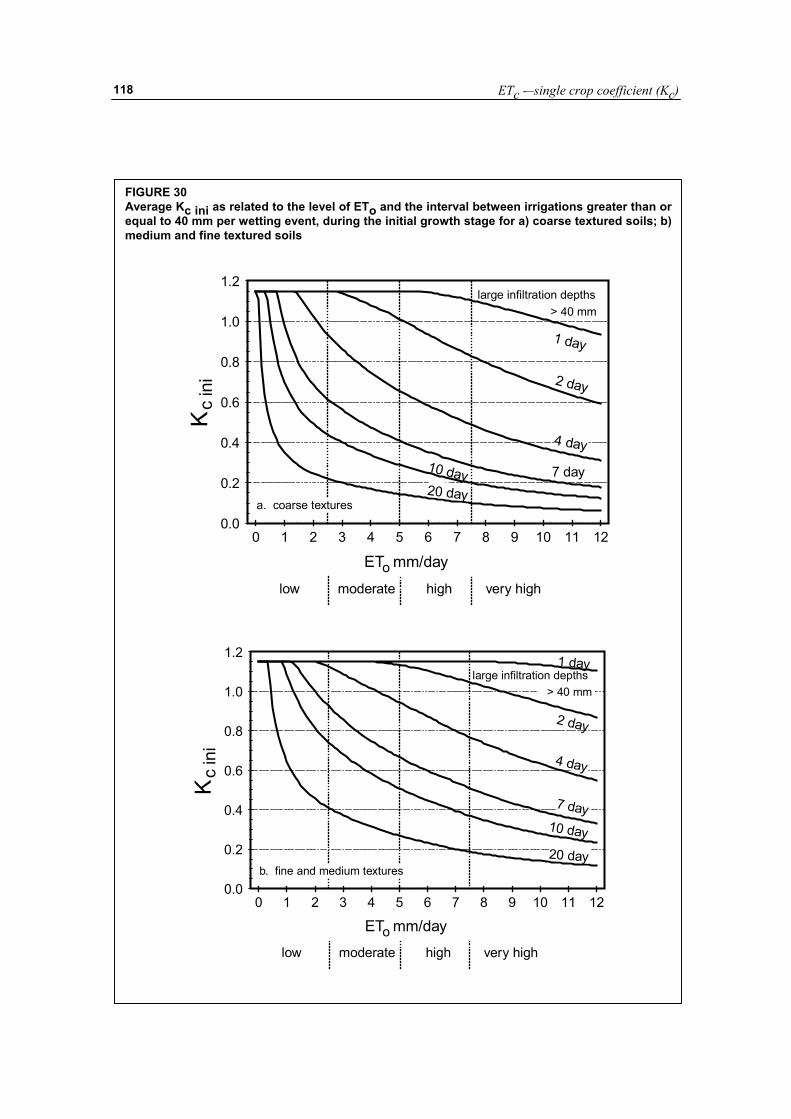
ETc -–single crop coefficient (Kc)
118
FIGURE 30 Average Kc ini as related to the level of ETo and the interval between irrigations greater than or equal to 40 mm per wetting event, during the initial growth stage for a) coarse textured soils; b) medium and fine textured soils
0 1 2 3 4 5 6 7 8 9 10 11 120.0
0.2
0.4
0.6
0.8
1.0
1.2
Kc
ini
ET mm/dayo
1 day
2 day
4 day
7 day10 day20 day
large infiltration depths> 40 mm
low moderate high very high
a. coarse textures
0 1 2 3 4 5 6 7 8 9 10 11 120.0
0.2
0.4
0.6
0.8
1.0
1.2
Kc
ini
ET mm/dayo
1 day
2 day
4 day
7 day10 day20 day
large infiltration depths > 40 mm
low moderate high very high
b. fine and medium textures
Crop evapotranspiration
119
EXAMPLE 25 Interpolation between light and heavy wetting events Small vegetables cultivated in a dry area on a coarse textured soil receive 20 mm of water twice a week by means of a sprinkler irrigation system. The average ETo during the initial stage is 5 mm/day. Estimate the crop evapotranspiration during that stage. For:
7/2 = ETo = and a coarse textured soil
3.5 5
day interval mm/day
From Fig. 29:
Kc ini(Fig. 29) ≈
0.55 -
From Fig. 30.a:
Kc ini(Fig. 30a) ≈ 0.7 -
For: I = 20 mm From Eq. 59:
Kc ini = 0.55 + [(20-10)/(40-10)] (0.7-0.55) = 0.55+0.33(0.15)=
0.60
-
From Eq. 58: ETc = 0.60 (5) = 3.0 mm/day The average crop evapotranspiration during the initial growth stage for the small vegetables is 3.0 mm/day.
Adjustment for partial wetting by irrigation Many types of irrigation systems wet only a fraction of the soil surface. For example, for a trickle irrigation system, the fraction of the surface wetted, fw, may be only 0.4. For furrow irrigation systems, the fraction of the surface wetted may range from 0.3 to 0.8. Common values for the fraction of the soil surface wetted by irrigation or precipitation are given in Table 20. When only a fraction of the soil surface is wetted, the value for Kc ini obtained from Table 12 or from Figures 29 or 30 should be multiplied by the fraction of the surface wetted to adjust for the partial wetting: Fig),(Tabinicwinic KfK = (60) where fw the fraction of surfaced wetted by irrigation or rain [0 - 1],
Kc ini (Tab,Fig) the value for Kc ini from Table 12 or Figure 29 or 30.
In addition, in selecting which figure to use (i.e., Figure 29 or 30), the average infiltrated depth, expressed in millimetres over the entire field surface, should be divided by fw to represent the true infiltrated depth of water for the part of the surface that is wetted (Figure 31):
w
w fII = (61)
where Iw irrigation depth for the part of the surface that is wetted [mm], fw fraction of surface wetted by irrigation, I the irrigation depth for the field [mm].
When irrigation of part of the soil surface and precipitation over the entire soil surface
both occur during the initial period, fw should represent the average of fw for each type of wetting, weighted according to the total infiltration depth received by each type.
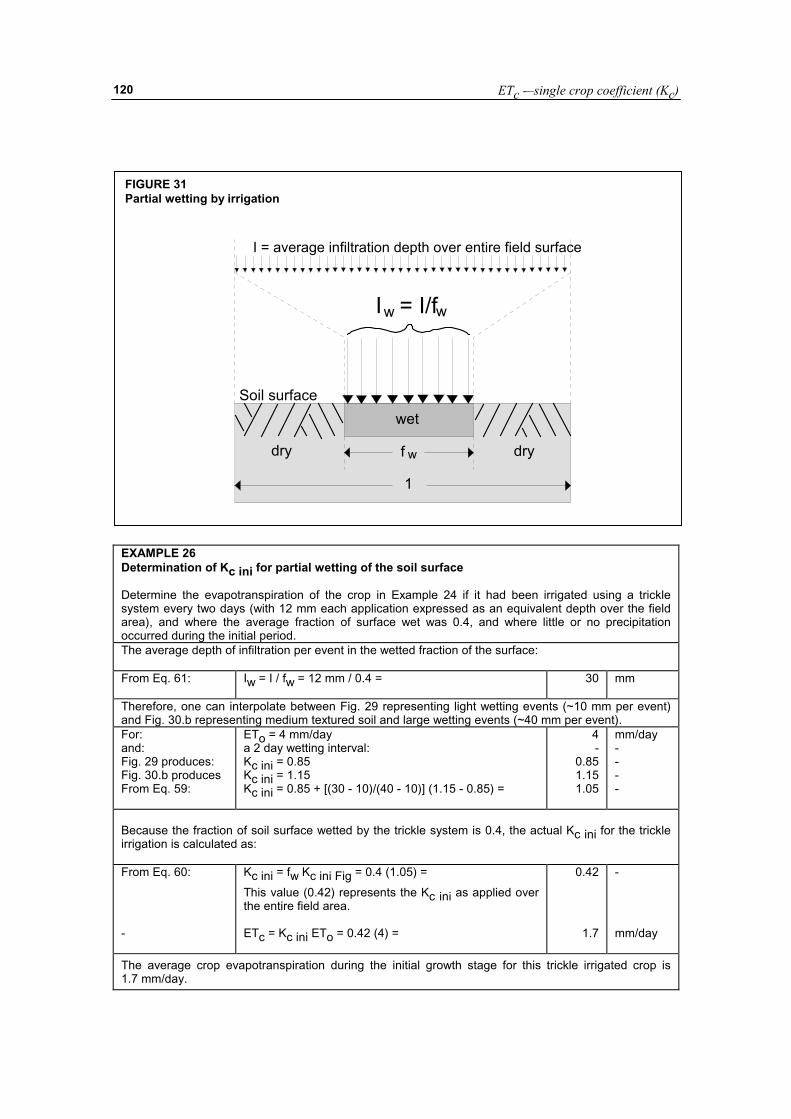
ETc -–single crop coefficient (Kc)
120
EXAMPLE 26 Determination of Kc ini for partial wetting of the soil surface Determine the evapotranspiration of the crop in Example 24 if it had been irrigated using a trickle system every two days (with 12 mm each application expressed as an equivalent depth over the field area), and where the average fraction of surface wet was 0.4, and where little or no precipitation occurred during the initial period. The average depth of infiltration per event in the wetted fraction of the surface: From Eq. 61:
Iw = I / fw = 12 mm / 0.4 =
30 mm
Therefore, one can interpolate between Fig. 29 representing light wetting events (~10 mm per event) and Fig. 30.b representing medium textured soil and large wetting events (~40 mm per event). For: and: Fig. 29 produces: Fig. 30.b produces From Eq. 59:
ETo = 4 mm/day a 2 day wetting interval: Kc ini = 0.85 Kc ini = 1.15 Kc ini = 0.85 + [(30 - 10)/(40 - 10)] (1.15 - 0.85) =
4 -
0.85 1.15 1.05
mm/day - - - -
Because the fraction of soil surface wetted by the trickle system is 0.4, the actual Kc ini for the trickle irrigation is calculated as: From Eq. 60:
-
Kc ini = fw Kc ini Fig = 0.4 (1.05) =
This value (0.42) represents the Kc ini as applied over the entire field area. ETc = Kc ini ETo = 0.42 (4) =
0.42
1.7
-
mm/day
The average crop evapotranspiration during the initial growth stage for this trickle irrigated crop is 1.7 mm/day.
FIGURE 31 Partial wetting by irrigation
dry
Soil surfacewet
dryf w
1
I = average infiltration depth over entire field surface
I = I/fw w
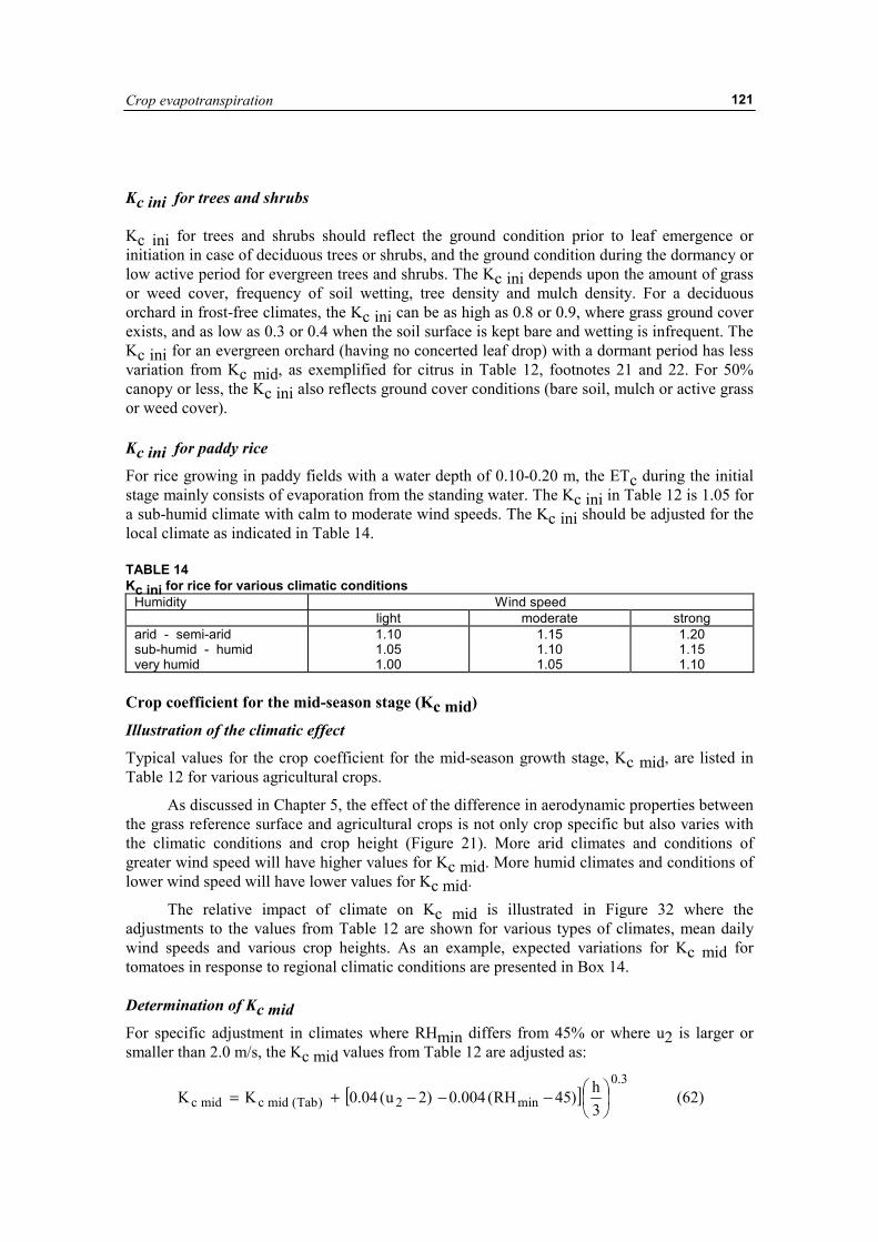
Crop evapotranspiration
121
Kc ini for trees and shrubs Kc ini for trees and shrubs should reflect the ground condition prior to leaf emergence or initiation in case of deciduous trees or shrubs, and the ground condition during the dormancy or low active period for evergreen trees and shrubs. The Kc ini depends upon the amount of grass or weed cover, frequency of soil wetting, tree density and mulch density. For a deciduous orchard in frost-free climates, the Kc ini can be as high as 0.8 or 0.9, where grass ground cover exists, and as low as 0.3 or 0.4 when the soil surface is kept bare and wetting is infrequent. The Kc ini for an evergreen orchard (having no concerted leaf drop) with a dormant period has less variation from Kc mid, as exemplified for citrus in Table 12, footnotes 21 and 22. For 50% canopy or less, the Kc ini also reflects ground cover conditions (bare soil, mulch or active grass or weed cover).
Kc ini for paddy rice
For rice growing in paddy fields with a water depth of 0.10-0.20 m, the ETc during the initial stage mainly consists of evaporation from the standing water. The Kc ini in Table 12 is 1.05 for a sub-humid climate with calm to moderate wind speeds. The Kc ini should be adjusted for the local climate as indicated in Table 14. TABLE 14 Kc ini for rice for various climatic conditions
Humidity Wind speed light moderate strong arid - semi-arid sub-humid - humid very humid
1.10 1.05 1.00
1.15 1.10 1.05
1.20 1.15 1.10
Crop coefficient for the mid-season stage (Kc mid)
Illustration of the climatic effect
Typical values for the crop coefficient for the mid-season growth stage, Kc mid, are listed in Table 12 for various agricultural crops.
As discussed in Chapter 5, the effect of the difference in aerodynamic properties between the grass reference surface and agricultural crops is not only crop specific but also varies with the climatic conditions and crop height (Figure 21). More arid climates and conditions of greater wind speed will have higher values for Kc mid. More humid climates and conditions of lower wind speed will have lower values for Kc mid.
The relative impact of climate on Kc mid is illustrated in Figure 32 where the adjustments to the values from Table 12 are shown for various types of climates, mean daily wind speeds and various crop heights. As an example, expected variations for Kc mid for tomatoes in response to regional climatic conditions are presented in Box 14. Determination of Kc mid
For specific adjustment in climates where RHmin differs from 45% or where u2 is larger or smaller than 2.0 m/s, the Kc mid values from Table 12 are adjusted as:
[ ]3.0
min2)Tab(midcmidc 3h)45RH(004.0)2u(04.0KK ��
���
�−−−+= (62)
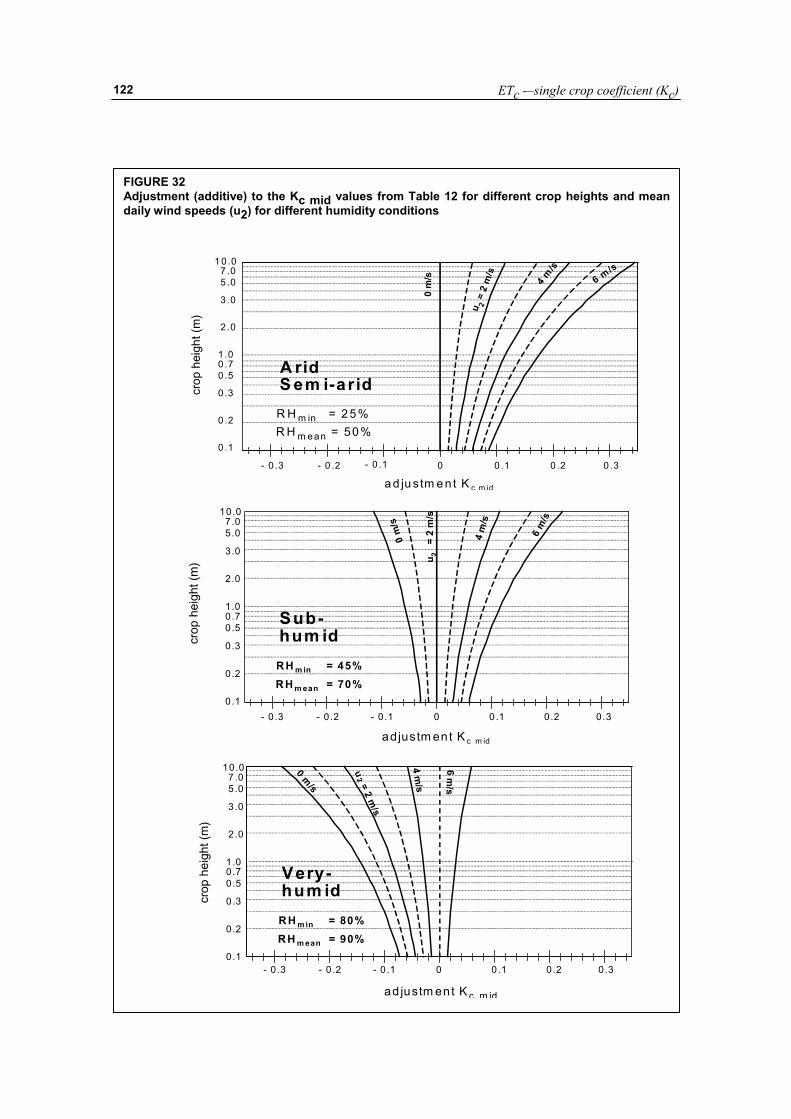
ETc -–single crop coefficient (Kc)
122
FIGURE 32 Adjustment (additive) to the Kc mid values from Table 12 for different crop heights and meandaily wind speeds (u2) for different humidity conditions
0 .1
0 .2
0 .3
0 .50 .71 .0
2 .0
3 .0
5 .07 .0
1 0 .0
R H m in = 2 5 %R H m ean = 50 %
- 0 .3 - 0 .2 - 0 .1 0 0 .1 0 .2 0 .3
a d ju s tm e nt K c m id
crop
hei
ght (
m)
0 m
/s 4 m/s
6 m/s
u 2 =
2 m
/s
A ridS em i-a rid
- 0 .3 - 0.2 - 0.1 0 0.1 0.2 0.3
adjustm ent K c m id
0.1
0.2
0.3
0.50.71.0
2.0
3.0
5.07.0
10.0
crop
hei
ght (
m)
R H m in = 45%R H m ean = 70%
Sub-hum id
0 m
/s
4 m
/s
6 m
/s
u 2 =
2 m
/s
0.1
0.2
0.3
0.50.71.0
2.0
3.0
5.07.0
10.0
crop
hei
ght (
m)
- 0 .3 - 0 .2 - 0 .1 0 0.1 0.2 0.3
ad justm ent K c m id
R H m in = 80%R H m ean = 90%
Very-hum id
0 m/s
4 m/s
6 m/s
u = 2 m/s
2
Crop evapotranspiration
123
where Kc mid (Tab) value for Kc mid taken from Table 12, u2 mean value for daily wind speed at 2 m height over grass during the mid-
season growth stage [m s-1], for 1 m s-1 ≤ u2 ≤ 6 m s-1, RHmin mean value for daily minimum relative humidity during the mid-season
growth stage [%], for 20% ≤ RHmin ≤ 80%, h mean plant height during the mid-season stage [m] for 0.1 m < h < 10 m.
The Kc mid values determined with equations 62 and 65 are average adjustments for the midseason and late season periods. The values for parameters u2 and RHmin should be accordingly taken as averages for these periods (see example, Annex 8). The limits expressed for parameters u2, RHmin and h should be observed.
BOX 14 Demonstration of effect of climate on Kc mid for wheat crop grown under field conditions From Table 12 for wheat: Kc mid = 1.15 and h = 1.0 m For semi-arid to arid conditions - for strong wind (4 m/s) Kc mid = 1.15 + 0.10 = 1.25 - for moderate wind (2 m/s) Kc mid = 1.15 + 0.05 = 1.20 - for calm wind (1 m/s) Kc mid = 1.15 + 0.00 = 1.17 For sub-humid conditions - for strong wind (4 m/s) Kc mid = 1.15 + 0.05 = 1.20 - for moderate wind (2 m/s) Kc mid = 1.15 + 0.00 = 1.15 - for calm wind (1 m/s) Kc mid = 1.15 - 0.05 = 1.12 For humid and very humid conditions - for strong wind (4 m/s) Kc mid = 1.15 - 0.05 = 1.10 - for moderate wind (2 m/s) Kc mid = 1.15 - 0.10 = 1.05 - for calm wind (1 m/s) Kc mid = 1.15 - 0.15 = 1.02 Depending on the aridity of the climate and the wind conditions, the crop coefficient for wheat during the mid-season stage ranges from 1.02 (humid and calm wind) to 1.25 (arid and strong wind).
Where the user does not have access to a calculator with an exponential function, the
solution of the (h/3)0.3 expression can be approximated as [(h/3)0.5]0.5 where the square root key is used.
RHmin is used rather than RHmean because it is easier to approximate RHmin from Tmax where relative humidity data are unavailable. Moreover, under the common condition where Tmin approaches Tdew (i.e., RHmax ≈ 100%), the vapour pressure deficit (es - ea), with es from Equation 12 and ea from Equation 17, becomes [(100-RHmin)/200] e°(Tmax), where e°(Tmax) is saturation vapour pressure at maximum daily air temperature. This indicates that RHmin better reflects the impact of vapour pressure deficit on Kc than does RHmean.
RHmin is calculated on a daily or average monthly basis as:
100)T(e
)T(eRH
maxo
dewo
min = (63)
where Tdew is mean dewpoint temperature and Tmax is mean daily maximum air temperature during the mid-season growth stage. Where dewpoint temperature or other hygrometric data are
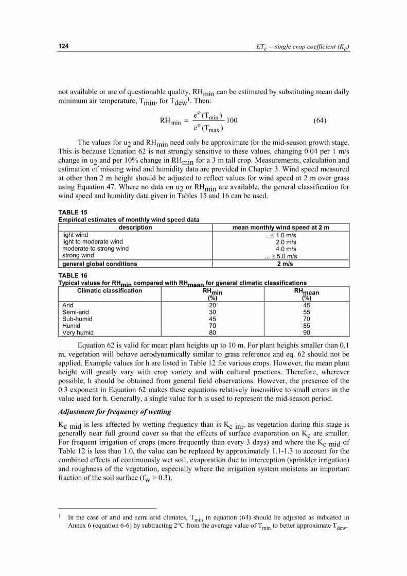
ETc -–single crop coefficient (Kc)
124
not available or are of questionable quality, RHmin can be estimated by substituting mean daily minimum air temperature, Tmin, for Tdew1. Then:
100)T(e
)T(eRH
maxo
mino
min = (64)
The values for u2 and RHmin need only be approximate for the mid-season growth stage. This is because Equation 62 is not strongly sensitive to these values, changing 0.04 per 1 m/s change in u2 and per 10% change in RHmin for a 3 m tall crop. Measurements, calculation and estimation of missing wind and humidity data are provided in Chapter 3. Wind speed measured at other than 2 m height should be adjusted to reflect values for wind speed at 2 m over grass using Equation 47. Where no data on u2 or RHmin are available, the general classification for wind speed and humidity data given in Tables 15 and 16 can be used. TABLE 15 Empirical estimates of monthly wind speed data
description mean monthly wind speed at 2 m light wind light to moderate wind moderate to strong wind strong wind
...≤ 1.0 m/s 2.0 m/s 4.0 m/s ... ≥ 5.0 m/s
general global conditions 2 m/s
TABLE 16 Typical values for RHmin compared with RHmean for general climatic classifications
Climatic classification RHmin (%)
RHmean (%)
Arid Semi-arid Sub-humid Humid Very humid
20 30 45 70 80
45 55 70 85 90
Equation 62 is valid for mean plant heights up to 10 m. For plant heights smaller than 0.1 m, vegetation will behave aerodynamically similar to grass reference and eq. 62 should not be applied. Example values for h are listed in Table 12 for various crops. However, the mean plant height will greatly vary with crop variety and with cultural practices. Therefore, wherever possible, h should be obtained from general field observations. However, the presence of the 0.3 exponent in Equation 62 makes these equations relatively insensitive to small errors in the value used for h. Generally, a single value for h is used to represent the mid-season period.
Adjustment for frequency of wetting
Kc mid is less affected by wetting frequency than is Kc ini, as vegetation during this stage is generally near full ground cover so that the effects of surface evaporation on Kc are smaller. For frequent irrigation of crops (more frequently than every 3 days) and where the Kc mid of Table 12 is less than 1.0, the value can be replaced by approximately 1.1-1.3 to account for the combined effects of continuously wet soil, evaporation due to interception (sprinkler irrigation) and roughness of the vegetation, especially where the irrigation system moistens an important fraction of the soil surface (fw > 0.3).
1 In the case of arid and semi-arid climates, Tmin in equation (64) should be adjusted as indicated in
Annex 6 (equation 6-6) by subtracting 2°C from the average value of Tmin to better approximate Tdew.
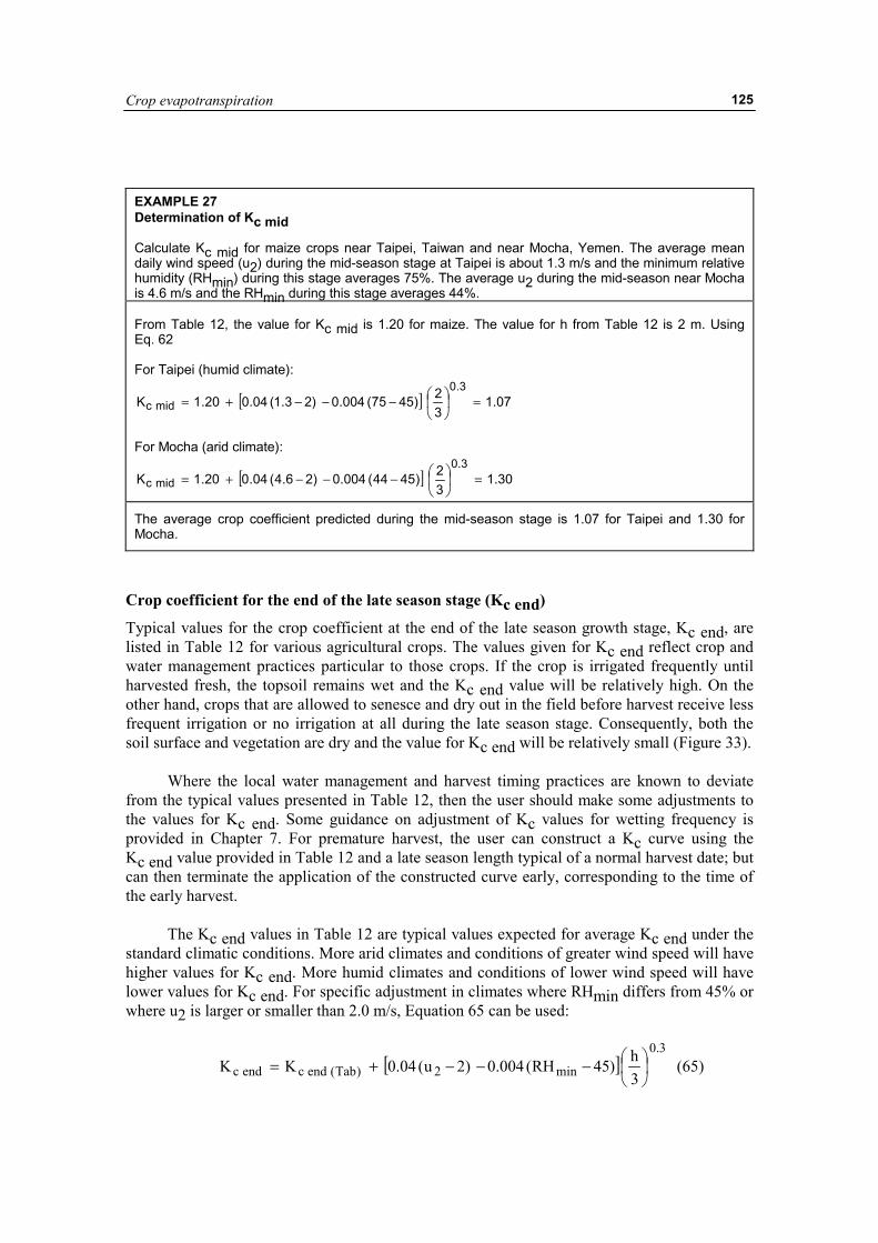
Crop evapotranspiration
125
EXAMPLE 27 Determination of Kc mid Calculate Kc mid for maize crops near Taipei, Taiwan and near Mocha, Yemen. The average mean daily wind speed (u2) during the mid-season stage at Taipei is about 1.3 m/s and the minimum relative humidity (RHmin) during this stage averages 75%. The average u2 during the mid-season near Mocha is 4.6 m/s and the RHmin during this stage averages 44%. From Table 12, the value for Kc mid is 1.20 for maize. The value for h from Table 12 is 2 m. Using Eq. 62 For Taipei (humid climate):
[ ] 07.132)4575(004.0)23.1(04.020.1K
3.0midc =�
�
���
�−−−+=
For Mocha (arid climate):
[ ] 30.132)4544(004.0)26.4(04.020.1K
3.0midc =�
�
���
�−−−+=
The average crop coefficient predicted during the mid-season stage is 1.07 for Taipei and 1.30 for Mocha.
Crop coefficient for the end of the late season stage (Kc end)
Typical values for the crop coefficient at the end of the late season growth stage, Kc end, are listed in Table 12 for various agricultural crops. The values given for Kc end reflect crop and water management practices particular to those crops. If the crop is irrigated frequently until harvested fresh, the topsoil remains wet and the Kc end value will be relatively high. On the other hand, crops that are allowed to senesce and dry out in the field before harvest receive less frequent irrigation or no irrigation at all during the late season stage. Consequently, both the soil surface and vegetation are dry and the value for Kc end will be relatively small (Figure 33).
Where the local water management and harvest timing practices are known to deviate from the typical values presented in Table 12, then the user should make some adjustments to the values for Kc end. Some guidance on adjustment of Kc values for wetting frequency is provided in Chapter 7. For premature harvest, the user can construct a Kc curve using the Kc end value provided in Table 12 and a late season length typical of a normal harvest date; but can then terminate the application of the constructed curve early, corresponding to the time of the early harvest.
The Kc end values in Table 12 are typical values expected for average Kc end under the
standard climatic conditions. More arid climates and conditions of greater wind speed will have higher values for Kc end. More humid climates and conditions of lower wind speed will have lower values for Kc end. For specific adjustment in climates where RHmin differs from 45% or where u2 is larger or smaller than 2.0 m/s, Equation 65 can be used:
[ ]3.0
min2)Tab(endcendc 3h)45RH(004.0)2u(04.0KK ��
���
�−−−+= (65)
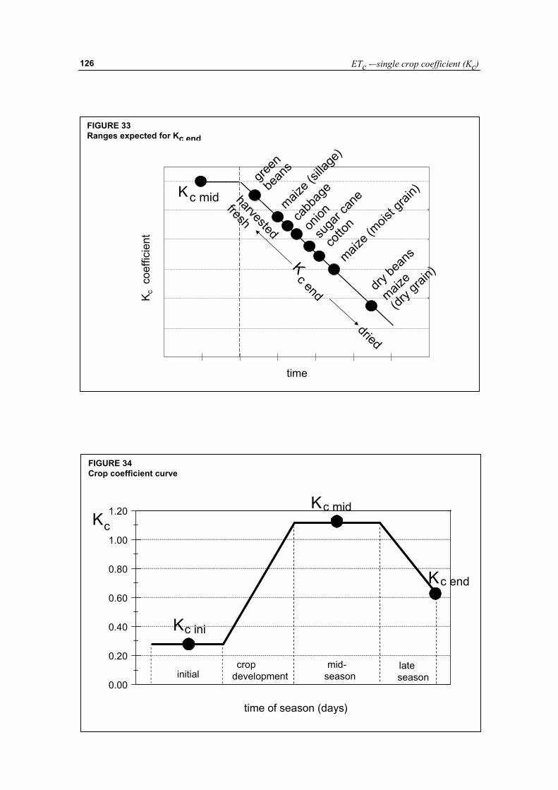
ETc -–single crop coefficient (Kc)
126
FIGURE 33 Ranges expected for Kc end
time
K c c
oeffi
cien
t
c midKca
bbag
e
onion
cotto
nsu
gar c
ane
maize (
sillag
e)
green
bean
s
maize (
moist g
rain)
dry be
ans
maize
(dry g
rain)
harvested
freshdried
c end
K
FIGURE 34 Crop coefficient curve
Kc
K
time of season (days)
0.00
0.20
0.40
0.60
0.80
1.00
1.20
K
K
initial cropdevelopment
mid-season
lateseason
c ini
c mid
c end
Crop evapotranspiration
127
where Kc end (Tab) value for Kc end taken from Table 12, u2 mean value for daily wind speed at 2 m height over grass during
the late season growth stage [m s-1], for 1 m s-1 ≤ u2 ≤ 6 m s-1, RHmin mean value for daily minimum relative humidity during the late
season stage [%],for 20% ≤ RHmin ≤ 80%, h mean plant height during the late season stage [m], for 0.1 m ≤ h
≤ 10 m.
Equation 65 is only applied when the tabulated values for Kc end exceed 0.45. The equation reduces the Kc end with increasing RHmin. This reduction in Kc end is characteristic of crops that are harvested ‘green’ or before becoming completely dead and dry (i.e., Kc end ≥ 0.45).
No adjustment is made when Kc end (Table) < 0.45 (i.e., Kc end = Kc end (Tab)). When
crops are allowed to senesce and dry in the field (as evidenced by Kc end < 0.45), u2 and RHmin have less effect on Kc end and no adjustment is necessary. In fact, Kc end may decrease with decreasing RHmin for crops that are ripe and dry at the time of harvest, as lower relative humidity accelerates the drying process. CONSTRUCTION OF THE Kc CURVE
Annual crops
Only three point values for Kc are required to describe and to construct the Kc curve. The curve such as that shown in Figure 34 is constructed using the following three steps:
1. Divide the growing period into four general growth stages that describe crop phenology or development (initial, crop development, mid-season, and late season stage), determine the lengths of the growth stages, and identify the three Kc values that correspond to Kc ini, Kc mid and Kc end from Table 12.
2. Adjust the Kc values to the frequency of wetting and/or climatic conditions of the growth stages as outlined in the previous section.
3. Construct a curve by connecting straight line segments through each of the four growth stages. Horizontal lines are drawn through Kc ini in the initial stage and through Kc mid in the mid-season stage. Diagonal lines are drawn from Kc ini to Kc mid within the course of the crop development stage and from Kc mid to Kc end within the course of the late season stage.
Kc curves for forage crops Many crops grown for forage or hay are harvested several times during the growing season. Each harvest essentially terminates a ‘sub’ growing season and associated Kc curve and initiates a new ‘sub’ growing season and associated Kc curve. The resulting Kc curve for the entire growing season is the aggregation of a series of Kc curves associated with each sub-cycle. Figure 35 presents a Kc curve for the entire growing season constructed for alfalfa grown for hay in southern Idaho.
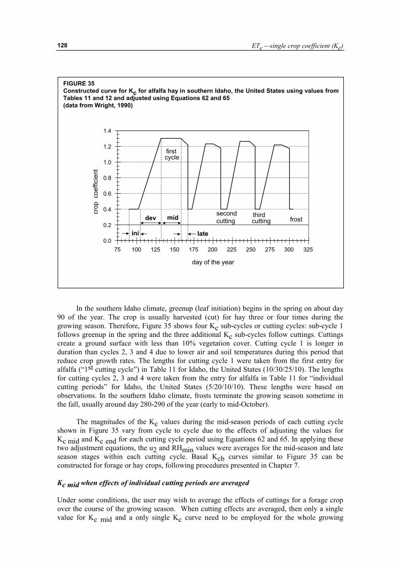
ETc -–single crop coefficient (Kc)
128
In the southern Idaho climate, greenup (leaf initiation) begins in the spring on about day 90 of the year. The crop is usually harvested (cut) for hay three or four times during the growing season. Therefore, Figure 35 shows four Kc sub-cycles or cutting cycles: sub-cycle 1 follows greenup in the spring and the three additional Kc sub-cycles follow cuttings. Cuttings create a ground surface with less than 10% vegetation cover. Cutting cycle 1 is longer in duration than cycles 2, 3 and 4 due to lower air and soil temperatures during this period that reduce crop growth rates. The lengths for cutting cycle 1 were taken from the first entry for alfalfa (“1st cutting cycle”) in Table 11 for Idaho, the United States (10/30/25/10). The lengths for cutting cycles 2, 3 and 4 were taken from the entry for alfalfa in Table 11 for “individual cutting periods” for Idaho, the United States (5/20/10/10). These lengths were based on observations. In the southern Idaho climate, frosts terminate the growing season sometime in the fall, usually around day 280-290 of the year (early to mid-October).
The magnitudes of the Kc values during the mid-season periods of each cutting cycle shown in Figure 35 vary from cycle to cycle due to the effects of adjusting the values for Kc mid and Kc end for each cutting cycle period using Equations 62 and 65. In applying these two adjustment equations, the u2 and RHmin values were averages for the mid-season and late season stages within each cutting cycle. Basal Kcb curves similar to Figure 35 can be constructed for forage or hay crops, following procedures presented in Chapter 7. Kc mid when effects of individual cutting periods are averaged Under some conditions, the user may wish to average the effects of cuttings for a forage crop over the course of the growing season. When cutting effects are averaged, then only a single value for Kc mid and a only single Kc curve need to be employed for the whole growing
FIGURE 35 Constructed curve for Kc for alfalfa hay in southern Idaho, the United States using values from Tables 11 and 12 and adjusted using Equations 62 and 65 (data from Wright, 1990)
75 100 125 150 175 200 225 250 275 300 325
day of the year
0.0
0.2
0.4
0.6
0.8
1.0
1.2
1.4
crop
coe
ffici
ent
ini
dev mid
late
secondcutting
thirdcutting frost
firstcycle
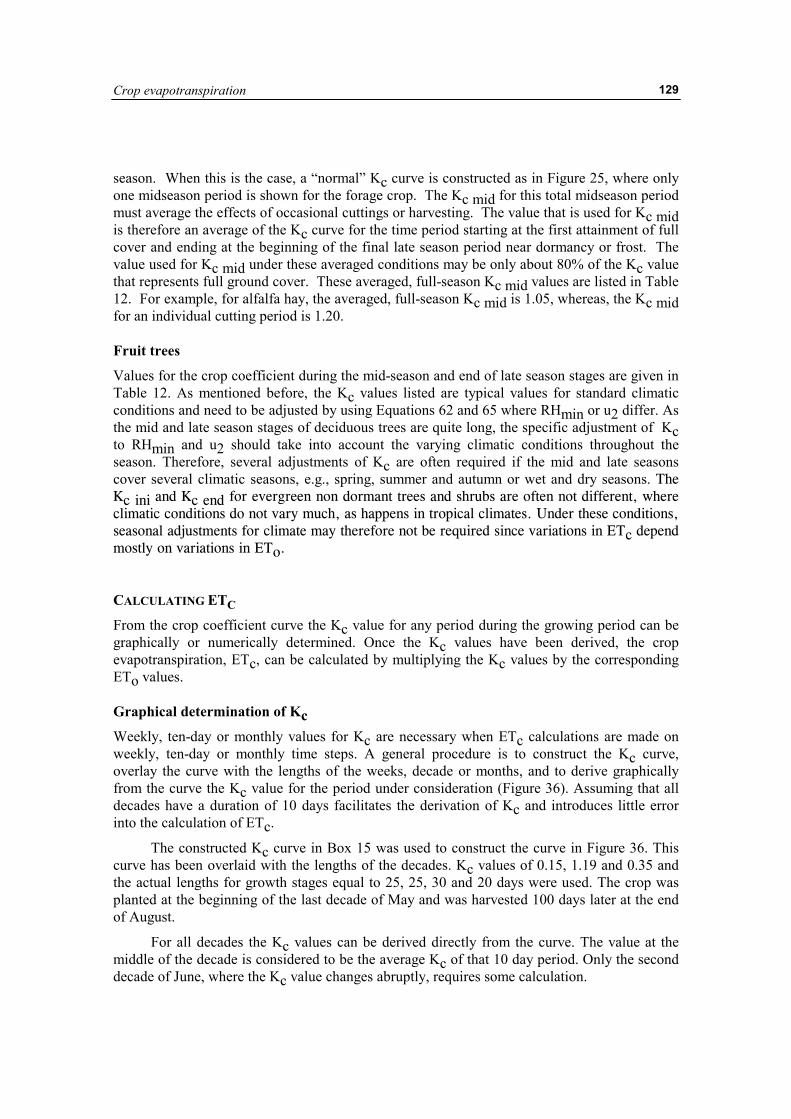
Crop evapotranspiration
129
season. When this is the case, a “normal” Kc curve is constructed as in Figure 25, where only one midseason period is shown for the forage crop. The Kc mid for this total midseason period must average the effects of occasional cuttings or harvesting. The value that is used for Kc mid is therefore an average of the Kc curve for the time period starting at the first attainment of full cover and ending at the beginning of the final late season period near dormancy or frost. The value used for Kc mid under these averaged conditions may be only about 80% of the Kc value that represents full ground cover. These averaged, full-season Kc mid values are listed in Table 12. For example, for alfalfa hay, the averaged, full-season Kc mid is 1.05, whereas, the Kc mid for an individual cutting period is 1.20. Fruit trees
Values for the crop coefficient during the mid-season and end of late season stages are given in Table 12. As mentioned before, the Kc values listed are typical values for standard climatic conditions and need to be adjusted by using Equations 62 and 65 where RHmin or u2 differ. As the mid and late season stages of deciduous trees are quite long, the specific adjustment of Kc to RHmin and u2 should take into account the varying climatic conditions throughout the season. Therefore, several adjustments of Kc are often required if the mid and late seasons cover several climatic seasons, e.g., spring, summer and autumn or wet and dry seasons. The Kc ini and Kc end for evergreen non dormant trees and shrubs are often not different, where climatic conditions do not vary much, as happens in tropical climates. Under these conditions, seasonal adjustments for climate may therefore not be required since variations in ETc depend mostly on variations in ETo. CALCULATING ETC
From the crop coefficient curve the Kc value for any period during the growing period can be graphically or numerically determined. Once the Kc values have been derived, the crop evapotranspiration, ETc, can be calculated by multiplying the Kc values by the corresponding ETo values. Graphical determination of Kc
Weekly, ten-day or monthly values for Kc are necessary when ETc calculations are made on weekly, ten-day or monthly time steps. A general procedure is to construct the Kc curve, overlay the curve with the lengths of the weeks, decade or months, and to derive graphically from the curve the Kc value for the period under consideration (Figure 36). Assuming that all decades have a duration of 10 days facilitates the derivation of Kc and introduces little error into the calculation of ETc.
The constructed Kc curve in Box 15 was used to construct the curve in Figure 36. This curve has been overlaid with the lengths of the decades. Kc values of 0.15, 1.19 and 0.35 and the actual lengths for growth stages equal to 25, 25, 30 and 20 days were used. The crop was planted at the beginning of the last decade of May and was harvested 100 days later at the end of August.
For all decades the Kc values can be derived directly from the curve. The value at the middle of the decade is considered to be the average Kc of that 10 day period. Only the second decade of June, where the Kc value changes abruptly, requires some calculation.
ETc -–single crop coefficient (Kc)
130
BOX 15 Case study of a dry bean crop at Kimberly, Idaho, the United States (single crop coefficient) An example application for using the Kc procedure under average soil wetness conditions is presented for a dry bean crop planted on 23 May 1974 at Kimberly, Idaho, the United States (latitude = 42.4°N). The initial, development, mid-season and late season stage lengths are taken from Table 11 for a continental climate as 20, 30, 40 and 20 days (the stage lengths listed for southern Idaho were not used in this example in order to demonstrate the only approximate accuracy of values provided in Table 11 when values for the specific location are not available). Initial values for Kc ini, Kc mid and Kc end are selected from Table 12 as 0.4, 1.15, and 0.35. The mean RHmin and u2 during both the mid-season and late season growth stages were 30% and 2.2 m/s. The maximum height suggested in Table 12 for dry beans is 0.4 m. Therefore, Kc mid is adjusted using Eq. 62 as:
[ ] 19.134.0)4530(004.0)22.2(04.015.1K
3.0midc =�
�
���
�−−−+=
As Kc end = 0.35 is less than 0.45, no adjustment is made to Kc end. The value for Kc mid is not significantly different from that in Table 12 as u2 ≈ 2 m/s, RHmin is just 15% lower than the 45% represented in Table 12, and the height of the beans is relatively short. The initial Kc curve for dry beans in Idaho can be drawn, for initial, planning purposes, as shown in the graph (dotted line), where Kc ini, Kc mid and Kc end are 0.4, 1.19, and 0.35 and the four lengths of growth stages are 20, 30, 40 and 20 days. Note that the Kc ini = 0.4 taken from Table 12 serves only as an initial, approximate estimate for Kc ini.
140 160 180 200 220 2400.00.20.40.60.81.01.21.41.6
0
40
80
120
160
200
day of the Year
Measured
crop
coe
ffici
ent
I
P
II
I
III
P
precipitation and irrigation (mm
)
Constructed Kc curves using values from Tables 11 and 12 directly (dotted line) and modified using Kc ini from Fig. 29 and Lini = 25, Ldev = 25, Lmid = 30, and Llate = 20 days (heavy line) for dry beans at Kimberly, Idaho. Also shown are daily measured Kc (lysimeter data from Wright, 1990).
Crop evapotranspiration
131
Kc ini can be more accurately estimated using the approach described in this chapter. ETo during the initial period at Kimberly (late May - early June, 1974) averaged 5.3 mm/day, and the wetting interval during this period was approximately 14 days (2 rainfall events occurred averaging 5 mm per event). Therefore, as the wetting events were light (< 10 mm each), Fig. 29 is used. The soil texture at Kimberly, Idaho is silt loam. From Fig. 29, Kc ini for the 14 day wetting interval and ETo = 5.3 mm/day is about 0.15. This value is substantially less than the general 0.4 value suggested by Table 12, and emphasizes the need to utilize local, actual precipitation and irrigation data when determining Kc ini.
Comparison of constructed curves with measurements
Because the ETc data for the dry bean crop at Kimberly, Idaho were measured using a precision lysimeter system during 1974 by Wright (1990), the actual Kc measurements can be compared with the constructed Kc curves, where actual Kc was calculated by dividing lysimeter measurements of ETc by daily ETo estimated using the FAO Penman-Monteith equation.
As illustrated in the graph, the mid-season length as taken from Table 11 for the general, continental climate overestimated the true mid-season length for dry beans in southern Idaho, which averaged only about 30 days rather than 40 days as suggested by Table 11. This illustrates the importance of using the local observation of 30 days for mid-season period length rather than the general value from Table 11.
The final, best estimate for the Kc curve for the dry bean crop in southern Idaho is plotted (lower curve in graph) using Kc values of 0.15, 1.19, and 0.35 and the actual observed lengths of growth stages equal to 25, 25, 30 and 20 days. Note the impact that the error in estimating mid-season length has on the area under the Kc curve. This supports the need to obtain local observations of growth stage dates and lengths.
The value calculated for Kc mid (1.19) appears to have underestimated the measured value for Kc during portions of the mid-season period at Kimberly. Some of this effect was due to effects of increased soil water evaporation following four irrigations during the 1974 mid-season which increased the effective Kc. This is illustrated in Box 16, where the basal Kcb + Ke approach is introduced and demonstrated for this same example.
The 0.15 value calculated for Kc ini using Fig. 29 agrees closely with measured Kc during the initial period. Measured Kc during the development period exceeded the final Kc curve during days on or following wetting events. The day to day variation in the lysimeter measured Kc is normal and is caused by day to day variations in weather, in wind direction, by errors in prediction of Rn and ETo, and by some random errors in the lysimeter measurements and weather measurements.
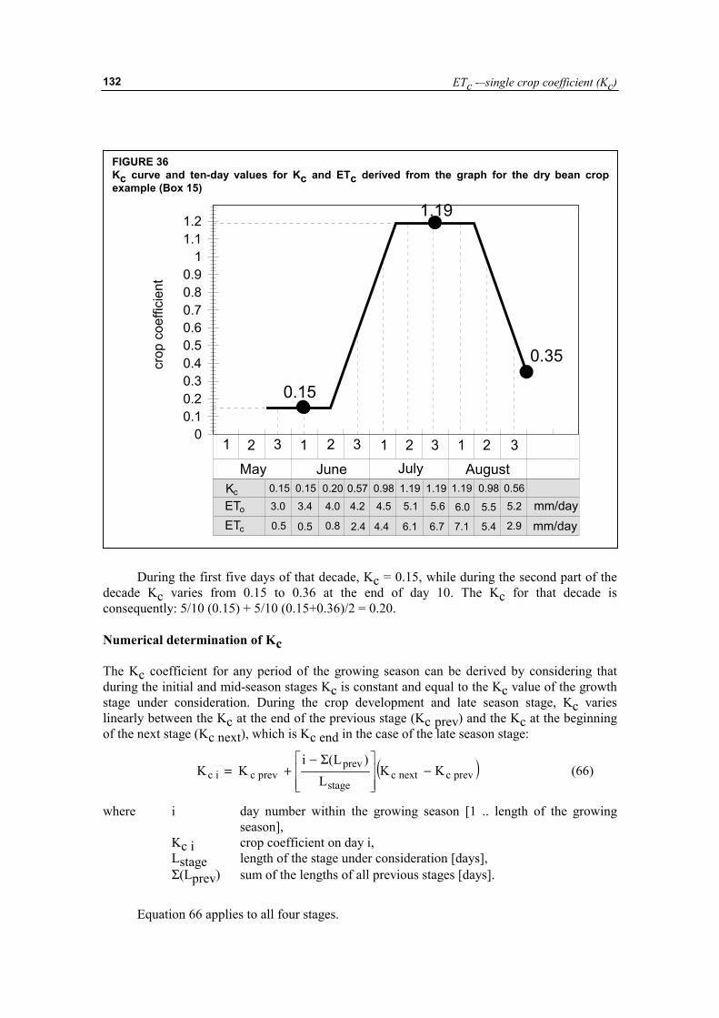
ETc -–single crop coefficient (Kc)
132
During the first five days of that decade, Kc = 0.15, while during the second part of the decade Kc varies from 0.15 to 0.36 at the end of day 10. The Kc for that decade is consequently: 5/10 (0.15) + 5/10 (0.15+0.36)/2 = 0.20.
Numerical determination of Kc The Kc coefficient for any period of the growing season can be derived by considering that during the initial and mid-season stages Kc is constant and equal to the Kc value of the growth stage under consideration. During the crop development and late season stage, Kc varies linearly between the Kc at the end of the previous stage (Kc prev) and the Kc at the beginning of the next stage (Kc next), which is Kc end in the case of the late season stage:
( )prevcnextcstage
prevprevcic KK
L)L(i
KK −���
�
���
� Σ−+= (66)
where i day number within the growing season [1 .. length of the growing season],
Kc i crop coefficient on day i, Lstage length of the stage under consideration [days], Σ(Lprev) sum of the lengths of all previous stages [days].
Equation 66 applies to all four stages.
FIGURE 36 Kc curve and ten-day values for Kc and ETc derived from the graph for the dry bean crop example (Box 15)
00.10.20.30.40.50.60.70.80.9
11.11.2
crop
coe
ffici
ent
1 2 3 1 2 3 1 2 3 1 2 3May June July August
mm/daymm/day
Kc
ETo
ETc
0.15
1.19
0.35
0.15 0.15 0.20 0.57 0.98 1.19 1.19 1.19 0.98 0.563.0 3.4 4.0 4.2 4.5 5.1 5.6 6.0 5.5 5.2
0.5 0.5 0.8 2.4 4.4 6.1 6.7 7.1 5.4 2.9
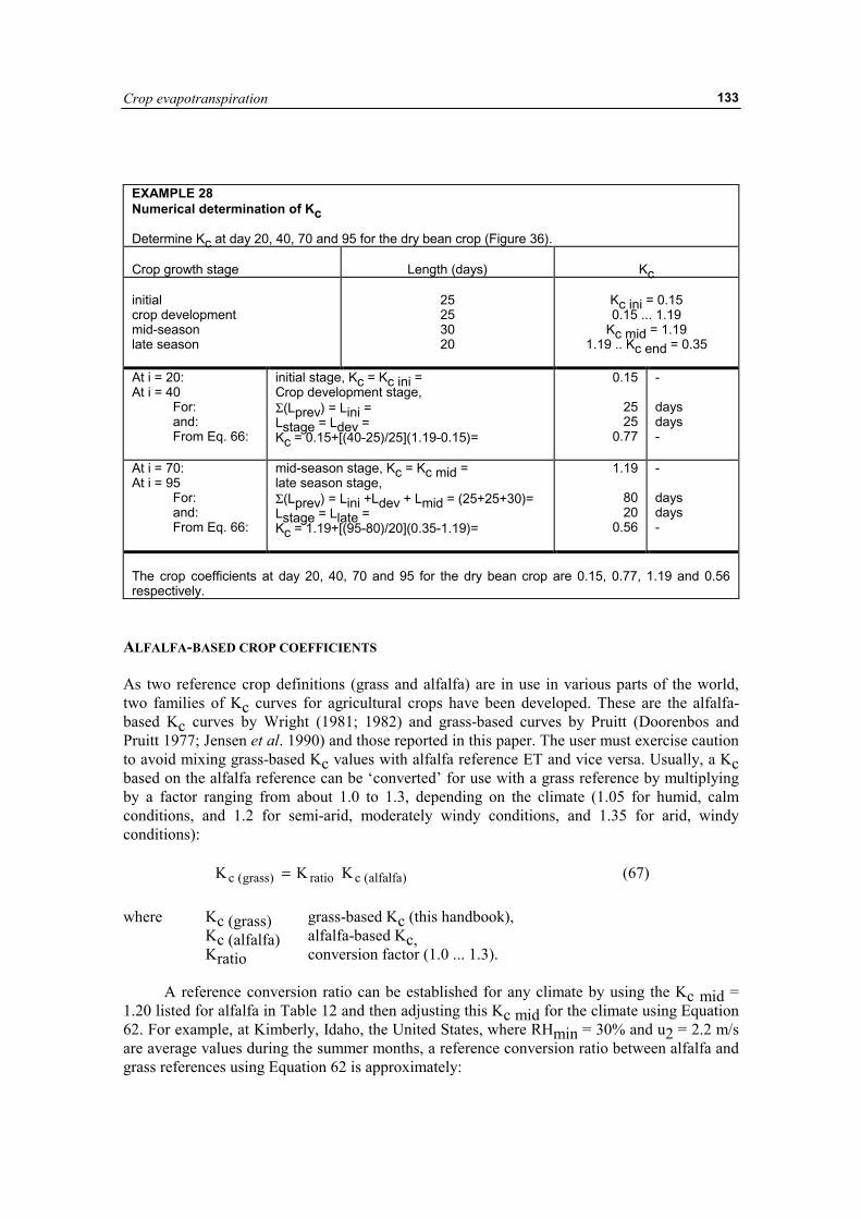
Crop evapotranspiration
133
EXAMPLE 28 Numerical determination of Kc Determine Kc at day 20, 40, 70 and 95 for the dry bean crop (Figure 36). Crop growth stage
Length (days)
Kc
initial crop development mid-season late season
25 25 30 20
Kc ini = 0.15 0.15 ... 1.19
Kc mid = 1.19 1.19 .. Kc end = 0.35
At i = 20: At i = 40 For: and: From Eq. 66:
initial stage, Kc = Kc ini = Crop development stage, Σ(Lprev) = Lini = Lstage = Ldev = Kc = 0.15+[(40-25)/25](1.19-0.15)=
0.15
25 25
0.77
- days days -
At i = 70: At i = 95 For: and: From Eq. 66:
mid-season stage, Kc = Kc mid = late season stage, Σ(Lprev) = Lini +Ldev + Lmid = (25+25+30)= Lstage = Llate = Kc = 1.19+[(95-80)/20](0.35-1.19)=
1.19
80 20
0.56
- days days -
The crop coefficients at day 20, 40, 70 and 95 for the dry bean crop are 0.15, 0.77, 1.19 and 0.56 respectively.
ALFALFA-BASED CROP COEFFICIENTS As two reference crop definitions (grass and alfalfa) are in use in various parts of the world, two families of Kc curves for agricultural crops have been developed. These are the alfalfa-based Kc curves by Wright (1981; 1982) and grass-based curves by Pruitt (Doorenbos and Pruitt 1977; Jensen et al. 1990) and those reported in this paper. The user must exercise caution to avoid mixing grass-based Kc values with alfalfa reference ET and vice versa. Usually, a Kc based on the alfalfa reference can be ‘converted’ for use with a grass reference by multiplying by a factor ranging from about 1.0 to 1.3, depending on the climate (1.05 for humid, calm conditions, and 1.2 for semi-arid, moderately windy conditions, and 1.35 for arid, windy conditions):
)alfalfa(cratio)grass(c KKK = (67) where Kc (grass) grass-based Kc (this handbook),
Kc (alfalfa) alfalfa-based Kc, Kratio conversion factor (1.0 ... 1.3).
A reference conversion ratio can be established for any climate by using the Kc mid =
1.20 listed for alfalfa in Table 12 and then adjusting this Kc mid for the climate using Equation 62. For example, at Kimberly, Idaho, the United States, where RHmin = 30% and u2 = 2.2 m/s are average values during the summer months, a reference conversion ratio between alfalfa and grass references using Equation 62 is approximately:
ETc -–single crop coefficient (Kc)
134
[ ] 24.135.0)4530(004.0)22.2(04.02.1K
3.0
ratio =��
���
�−−−+= (68)
where h = 0.5 m is the standard height for the alfalfa reference. TRANSFERABILITY OF PREVIOUS KC VALUES The values for Kc mid and Kc end listed in Table 12 are for a large part based on the original values presented in FAO Irrigation and Drainage Papers No. 24 and 33 (FAO-24 and FAO-33), with some adjustment and revisions to reflect recent findings. Similarly adjustments in Kc mid to compensate for differences in aerodynamic roughness and leaf area, as introduced in Equation 62 are derived from the Kc values given for different wind and RHmin conditions in the concerned Kc table in FAO-24, with some upward adjustment to better reflect increased ETcrop values under high wind and low RHmin when applied with the FAO Penman-Monteith equation.
The Kc’s from FAO-24 were based primarily on a living grass reference crop. The FAO Penman-Monteith equation presented in this publication similarly represents the same standardized grass reference. For that reason Kc values are in general not very different between these publications except under high wind and low RHmin.
The No. 24 modified Penman was found frequently to overestimate ETo even up to 25 % under high wind and low evaporative conditions and required often substantial local calibration (see chapter 2). Kc values derived from crop water use studies which used the FAO-24 Penman equation to compute grass reference crop evapotranspiration, can therefore not be used and need to be adjusted using ETo values estimated from the FAO Penman-Monteith equation. Similarly crop water requirement estimates based on the FAO-24 Modified Penman equation will need to be reassessed in view of the found differences between the FAO-24 Penman and the FAO Penman-Monteith reference equations.
Crop evapotranspiration
135
Chapter 7
ETc – dual crop coefficient (Kc = Kcb + Ke)
Like Chapter 6, this chapter also deals with the calculation of crop evapotranspiration (ETc) under standard conditions where no limitations are placed on crop growth or evapotranspiration. This chapter presents the procedure for predicting the effects of specific wetting events on the value for the crop coefficient Kc. The solution consists of splitting Kc into two separate coefficients, one for crop transpiration, i.e., the basal crop coefficient (Kcb), and one for soil evaporation (Ke): oecbc ET)K(KET += (69)
The dual crop coefficient approach is more complicated and more computationally intensive than the single crop coefficient approach (Kc) of Chapter 6. The procedure is conducted on a daily basis and is intended for applications using computers. It is recommended that the approach be followed when improved estimates for Kc are needed, for example to schedule irrigations for individual fields on a daily basis.
The calculation procedure for crop evapotranspiration, ETc, consists of: 1. identifying the lengths of crop growth stages, and selecting the corresponding Kcb
coefficients; 2. adjusting the selected Kcb coefficients for climatic conditions during the stage; 3. constructing the basal crop coefficient curve (allowing one to determine Kcb values for
any period during the growing period); 4. determining daily Ke values for surface evaporation; and 5. calculating ETc as the product of ETo and (Kcb + Ke). TRANSPIRATION COMPONENT (Kcb ETo)
Basal crop coefficient (Kcb)
The basal crop coefficient (Kcb) is defined as the ratio of the crop evapotranspiration over the reference evapotranspiration (ETc/ETo) when the soil surface is dry but transpiration is occurring at a potential rate, i.e., water is not limiting transpiration (Figure 22). Therefore, 'Kcb ETo' represents primarily the transpiration component of ETc. The Kcb ETo does include a residual diffusive evaporation component supplied by soil water below the dry surface and by soil water from beneath dense vegetation.
ETc -–dual crop coefficient (Kc = Kcb + Ke)
136
As the Kc values of Chapter 6 include averaged effects of evaporation from the soil surface, the Kcb values lie below the Kc values as illustrated in Figure 26 and a separate table for Kcb is required. Recommended values for Kcb are listed in Table 17 for the same crops listed in Table 12. As with Table 12, the values for Kcb in the table represent Kcb for a sub-humid climate and with moderate wind speed. For specific adjustment in climates where RHmin differs from 45% or where the wind speed is larger or smaller than 2 m/s, the Kcb mid and Kcb end values larger than 0.45 must be adjusted using the following equation:
[ ]3.0
min2)Tab(cbcb 3h)45RH(004.0)2u(04.0KK ��
���
�−−−+= (70)
where Kcb (Tab) the value for Kcb mid or Kcb end ( if ≥ 0.45) taken from Table 17, u2 the mean value for daily wind speed at 2 m height over grass during the
mid or late season growth stage [m s-1] for 1 m s-1 ≤ u2 ≤ 6 m s-1, RHmin the mean value for daily minimum relative humidity during the mid- or
late season growth stage [%] for 20% ≤ RHmin ≤ 80%, h the mean plant height during the mid or late season stage [m] (from
Table 12) for 20% ≤ RHmin ≤ 80%.
For a full discussion on the impact of the climatic correction, and the numerical determination of Kcb mid and Kcb end, the user is referred to the discussions on Kc mid and Kc end in Chapter 6.
Table 18 summarizes the general guidelines that were used in deriving Kcb values from the Kc values listed in Table 17. Where local research results are available, values for Kcb from Table 17 can be modified to reflect effects of local conditions, cultural practices or crop varieties on Kcb. However, local values for Kcb should not be expected to deviate by more than 0.2 from the values in Table 17. A greater deviation should signal the need to investigate or evaluate the local research technique, equipment and cultural practices. Where local Kcb values are used, no adjustment for climate using Equation 70 is necessary.
EXAMPLE 29 Selection and adjustment of basal crop coefficients, Kcb Select Kcb ini, Kcb mid and Kcb end for the dry bean crop of Box 15. Kcb ini, Kcb mid and Kcb end can be selected directly from Table 17 for dry beans as 0.15, 1.10 and 0.25. When adjusted for climate using Eq. 70: Kcb ini = 0.15 Kcb mid = 1.10 + (0.04 (2.2-2) - 0.004 (30-45) )(0.4/3)0.3 = 1.14 Kcb end = 0.25 (as Kcb < 0.45) Height for beans was taken from Table 12 as 0.4 m. The corresponding Kcb curve is shown in Figure 37.
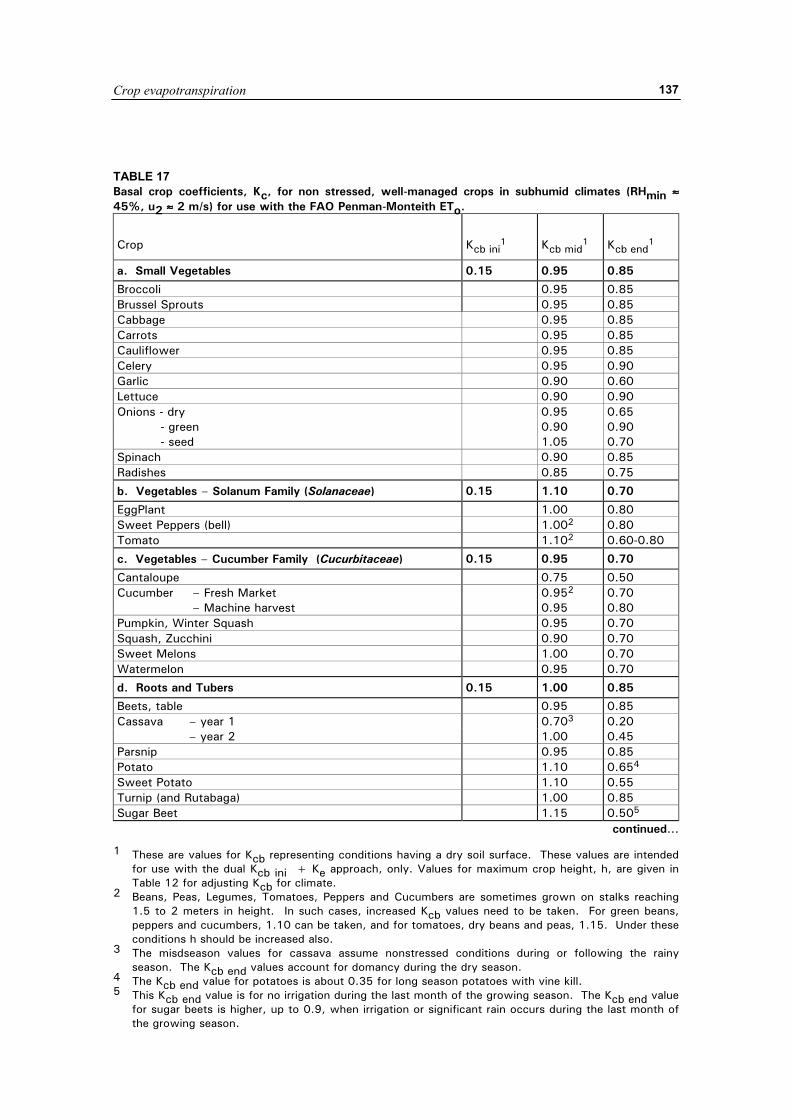
Crop evapotranspiration
137
TABLE 17 Basal crop coefficients, Kc, for non stressed, well-managed crops in subhumid climates (RHmin ≈≈≈≈ 45%, u2 ≈≈≈≈ 2 m/s) for use with the FAO Penman-Monteith ETo.
Crop
Kcb ini1
Kcb mid1
Kcb end1
a. Small Vegetables 0.15 0.95 0.85
Broccoli 0.95 0.85 Brussel Sprouts 0.95 0.85 Cabbage 0.95 0.85 Carrots 0.95 0.85 Cauliflower 0.95 0.85 Celery 0.95 0.90 Garlic 0.90 0.60 Lettuce 0.90 0.90 Onions - dry 0.95 0.65
- green 0.90 0.90 - seed 1.05 0.70
Spinach 0.90 0.85 Radishes 0.85 0.75
b. Vegetables – Solanum Family (Solanaceae) 0.15 1.10 0.70
EggPlant 1.00 0.80 Sweet Peppers (bell) 1.002 0.80 Tomato 1.102 0.60-0.80
c. Vegetables – Cucumber Family (Cucurbitaceae) 0.15 0.95 0.70
Cantaloupe 0.75 0.50 Cucumber – Fresh Market 0.952 0.70 – Machine harvest 0.95 0.80 Pumpkin, Winter Squash 0.95 0.70 Squash, Zucchini 0.90 0.70 Sweet Melons 1.00 0.70 Watermelon 0.95 0.70
d. Roots and Tubers 0.15 1.00 0.85
Beets, table 0.95 0.85 Cassava – year 1 0.703 0.20 – year 2 1.00 0.45 Parsnip 0.95 0.85 Potato 1.10 0.654 Sweet Potato 1.10 0.55 Turnip (and Rutabaga) 1.00 0.85 Sugar Beet 1.15 0.505
continued… 1 These are values for Kcb representing conditions having a dry soil surface. These values are intended
for use with the dual Kcb ini + Ke approach, only. Values for maximum crop height, h, are given in Table 12 for adjusting Kcb for climate.
2 Beans, Peas, Legumes, Tomatoes, Peppers and Cucumbers are sometimes grown on stalks reaching 1.5 to 2 meters in height. In such cases, increased Kcb values need to be taken. For green beans, peppers and cucumbers, 1.10 can be taken, and for tomatoes, dry beans and peas, 1.15. Under these conditions h should be increased also.
3 The misdseason values for cassava assume nonstressed conditions during or following the rainy season. The Kcb end values account for domancy during the dry season.
4 The Kcb end value for potatoes is about 0.35 for long season potatoes with vine kill. 5 This Kcb end value is for no irrigation during the last month of the growing season. The Kcb end value
for sugar beets is higher, up to 0.9, when irrigation or significant rain occurs during the last month of the growing season.
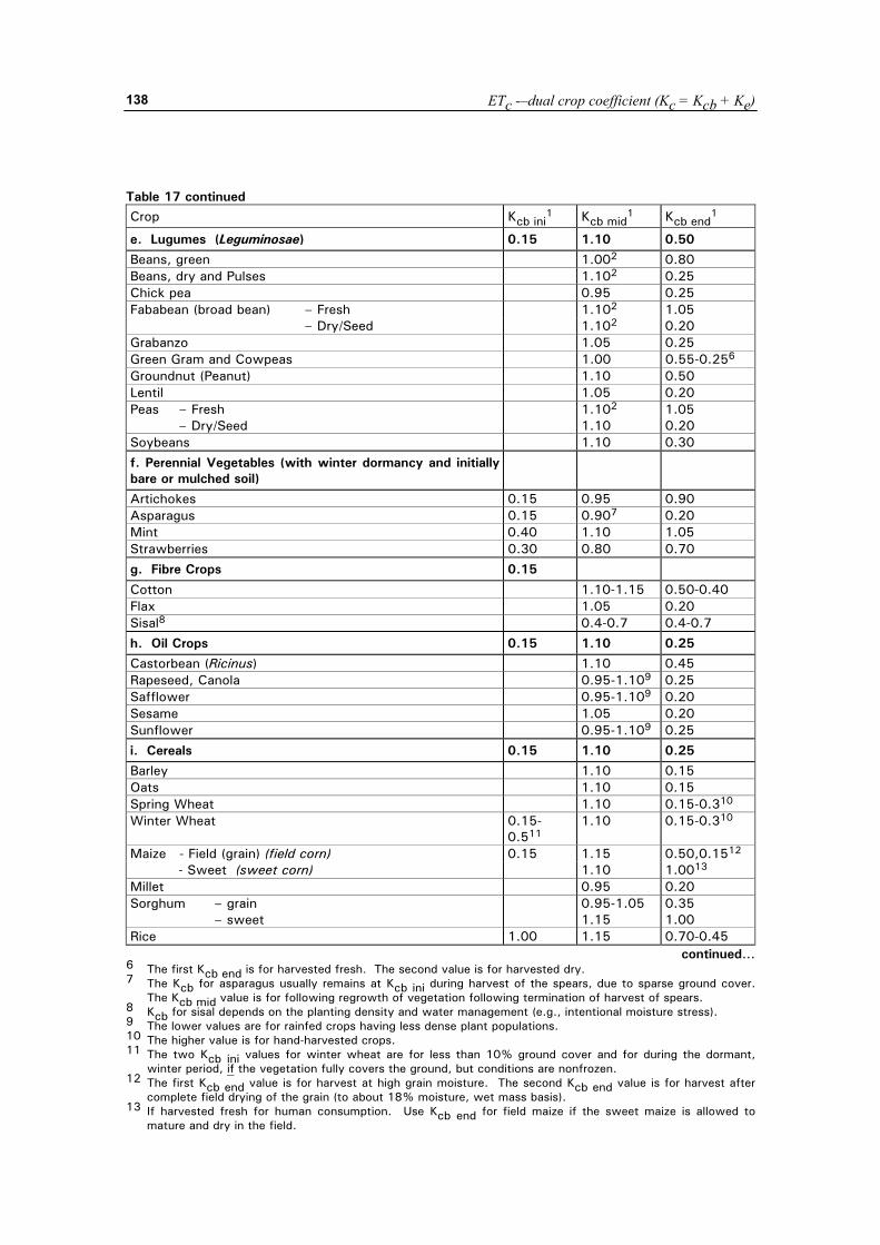
ETc -–dual crop coefficient (Kc = Kcb + Ke)
138
Table 17 continued Crop Kcb ini
1 Kcb mid1 Kcb end
1
e. Lugumes (Leguminosae) 0.15 1.10 0.50
Beans, green 1.002 0.80 Beans, dry and Pulses 1.102 0.25 Chick pea 0.95 0.25 Fababean (broad bean) – Fresh 1.102 1.05 – Dry/Seed 1.102 0.20 Grabanzo 1.05 0.25 Green Gram and Cowpeas 1.00 0.55-0.256 Groundnut (Peanut) 1.10 0.50 Lentil 1.05 0.20 Peas – Fresh 1.102 1.05 – Dry/Seed 1.10 0.20 Soybeans 1.10 0.30 f. Perennial Vegetables (with winter dormancy and initially bare or mulched soil)
Artichokes 0.15 0.95 0.90 Asparagus 0.15 0.907 0.20 Mint 0.40 1.10 1.05 Strawberries 0.30 0.80 0.70 g. Fibre Crops 0.15
Cotton 1.10-1.15 0.50-0.40 Flax 1.05 0.20 Sisal8 0.4-0.7 0.4-0.7 h. Oil Crops 0.15 1.10 0.25
Castorbean (Ricinus) 1.10 0.45 Rapeseed, Canola 0.95-1.109 0.25 Safflower 0.95-1.109 0.20 Sesame 1.05 0.20 Sunflower 0.95-1.109 0.25 i. Cereals 0.15 1.10 0.25
Barley 1.10 0.15 Oats 1.10 0.15 Spring Wheat 1.10 0.15-0.310
Winter Wheat 0.15-0.511
1.10 0.15-0.310
Maize - Field (grain) (field corn) 0.15 1.15 0.50,0.1512 - Sweet (sweet corn) 1.10 1.0013
Millet 0.95 0.20 Sorghum – grain 0.95-1.05 0.35 – sweet 1.15 1.00 Rice 1.00 1.15 0.70-0.45
continued… 6 The first Kcb end is for harvested fresh. The second value is for harvested dry. 7 The Kcb for asparagus usually remains at Kcb ini during harvest of the spears, due to sparse ground cover.
The Kcb mid value is for following regrowth of vegetation following termination of harvest of spears. 8 Kcb for sisal depends on the planting density and water management (e.g., intentional moisture stress). 9 The lower values are for rainfed crops having less dense plant populations. 10 The higher value is for hand-harvested crops. 11 The two Kcb ini values for winter wheat are for less than 10% ground cover and for during the dormant,
winter period, if the vegetation fully covers the ground, but conditions are nonfrozen. 12 The first Kcb end value is for harvest at high grain moisture. The second Kcb end value is for harvest after
complete field drying of the grain (to about 18% moisture, wet mass basis). 13 If harvested fresh for human consumption. Use Kcb end for field maize if the sweet maize is allowed to
mature and dry in the field.
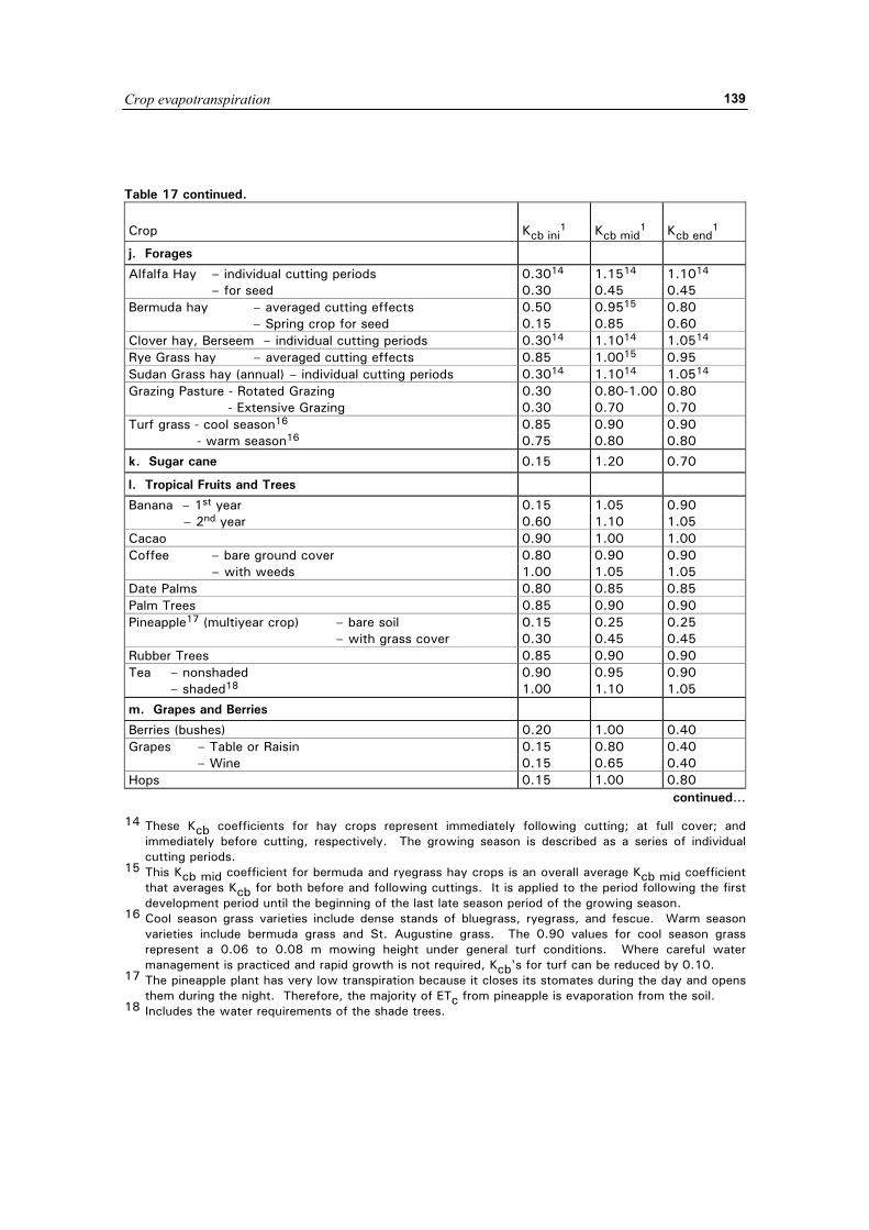
Crop evapotranspiration
139
Table 17 continued. Crop
Kcb ini
1 Kcb mid
1 Kcb end
1
j. Forages
Alfalfa Hay – individual cutting periods 0.3014 1.1514 1.1014 – for seed 0.30 0.45 0.45 Bermuda hay – averaged cutting effects 0.50 0.9515 0.80 – Spring crop for seed 0.15 0.85 0.60 Clover hay, Berseem – individual cutting periods 0.3014 1.1014 1.0514 Rye Grass hay – averaged cutting effects 0.85 1.0015 0.95 Sudan Grass hay (annual) – individual cutting periods 0.3014 1.1014 1.0514 Grazing Pasture - Rotated Grazing 0.30 0.80-1.00 0.80
- Extensive Grazing 0.30 0.70 0.70 Turf grass - cool season16 0.85 0.90 0.90
- warm season16 0.75 0.80 0.80
k. Sugar cane 0.15 1.20 0.70
l. Tropical Fruits and Trees
Banana – 1st year 0.15 1.05 0.90 – 2nd year 0.60 1.10 1.05 Cacao 0.90 1.00 1.00 Coffee – bare ground cover 0.80 0.90 0.90 – with weeds 1.00 1.05 1.05 Date Palms 0.80 0.85 0.85 Palm Trees 0.85 0.90 0.90 Pineapple17 (multiyear crop) – bare soil 0.15 0.25 0.25 – with grass cover 0.30 0.45 0.45 Rubber Trees 0.85 0.90 0.90 Tea – nonshaded 0.90 0.95 0.90 – shaded18 1.00 1.10 1.05
m. Grapes and Berries
Berries (bushes) 0.20 1.00 0.40 Grapes – Table or Raisin 0.15 0.80 0.40 – Wine 0.15 0.65 0.40 Hops 0.15 1.00 0.80
continued… 14 These Kcb coefficients for hay crops represent immediately following cutting; at full cover; and
immediately before cutting, respectively. The growing season is described as a series of individual cutting periods.
15 This Kcb mid coefficient for bermuda and ryegrass hay crops is an overall average Kcb mid coefficient that averages Kcb for both before and following cuttings. It is applied to the period following the first development period until the beginning of the last late season period of the growing season.
16 Cool season grass varieties include dense stands of bluegrass, ryegrass, and fescue. Warm season varieties include bermuda grass and St. Augustine grass. The 0.90 values for cool season grass represent a 0.06 to 0.08 m mowing height under general turf conditions. Where careful water management is practiced and rapid growth is not required, Kcb's for turf can be reduced by 0.10.
17 The pineapple plant has very low transpiration because it closes its stomates during the day and opens them during the night. Therefore, the majority of ETc from pineapple is evaporation from the soil.
18 Includes the water requirements of the shade trees.
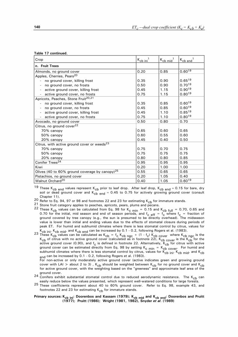
ETc -–dual crop coefficient (Kc = Kcb + Ke)
140
Table 17 continued.
Crop Kcb ini1 Kcb mid
1 Kcb end1
n. Fruit Trees
Almonds, no ground cover 0.20 0.85 0.6019 Apples, Cherries, Pears20 - no ground cover, killing frost 0.35 0.90 0.6519 - no ground cover, no frosts 0.50 0.90 0.7019 - active ground cover, killing frost 0.45 1.15 0.9019 - active ground cover, no frosts 0.75 1.15 0.8019 Apricots, Peaches, Stone Fruit20,21 - no ground cover, killing frost 0.35 0.85 0.6019 - no ground cover, no frosts 0.45 0.85 0.6019 - active ground cover, killing frost 0.45 1.10 0.8519 - active ground cover, no frosts 0.75 1.10 0.8019 Avocado, no ground cover 0.50 0.80 0.70 Citrus, no ground cover22 70% canopy 0.65 0.60 0.65 50% canopy 0.60 0.55 0.60 20% canopy 0.45 0.40 0.50 Citrus, with active ground cover or weeds23 70% canopy 0.75 0.70 0.75 50% canopy 0.75 0.75 0.75 20% canopy 0.80 0.80 0.85 Conifer Trees24 0.95 0.95 0.95 Kiwi 0.20 1.00 1.00 Olives (40 to 60% ground coverage by canopy)25 0.55 0.65 0.65 Pistachios, no ground cover 0.20 1.05 0.40 Walnut Orchard20 0.40 1.05 0.6019
19 These Kcb end values represent Kcb prior to leaf drop. After leaf drop, Kcb end ≈ 0.15 for bare, dry soil or dead ground cover and Kcb end ≈ 0.45 to 0.75 for actively growing ground cover (consult Chapter 11).
20 Refer to Eq. 94, 97 or 98 and footnotes 22 and 23 for estimating Kcb for immature stands. 21 Stone fruit category applies to peaches, apricots, pears, plums and pecans. 22 These Kcb values can be calculated from Eq. 98 for Kc min = 0.15 and Kcb full = 0.70, 0.65 and
0.70 for the initial, mid season and end of season periods, and fc eff = fc where fc = fraction of ground covered by tree canopy (e.g., the sun is presumed to be directly overhead). The midseason value is lower than initial and ending values due to the effects of stomatal closure during periods of peak ET. For humid and subhumid climates where there is less stomatal control by citrus, values for Kcb ini, Kcb mid, and Kcb end can be increased by 0.1 - 0.2, following Rogers et al. (1983).
23 These Kcb values can be calculated as Kcb = fc Kcb ngc + (1 - fc) Kcb cover where Kcb ngc is the Kcb of citrus with no active ground cover (calculated as in footnote 22), Kcb cover is the Kcb for the active ground cover (0.90), and fc is defined in footnote 22. Alternatively, Kcb for citrus with active ground cover can be estimated directly from Eq. 98 by setting Kc min = Kcb cover. For humid and subhumid climates where there is less stomatal control by citrus, values for Kcb ini, Kcb mid, and Kcb end can be increased by 0.1 - 0.2, following Rogers et al. (1983).
For non-active or only moderately active ground cover (active indicates green and growing ground cover with LAI > about 2 to 3) , Kcb should be weighted between Kcb for no ground cover and Kcb for active ground cover, with the weighting based on the "greeness" and approximate leaf area of the ground cover.
24 Conifers exhibit substantial stomatal control due to reduced aerodynamic resistance. The Kcb can easily reduce below the values presented, which represent well-watered conditions for large forests.
25 These coefficients represent about 40 to 60% ground cover. Refer to Eq. 98, example 43, and footnotes 22 and 23 for estimating Kcb for immature stands.
Primary sources: Kcb ini: Doorenbos and Kassam (1979); Kcb mid and Kcb end: Doorenbos and Pruitt (1977); Pruitt (1986); Wright (1981, 1982), Snyder et al. (1989)
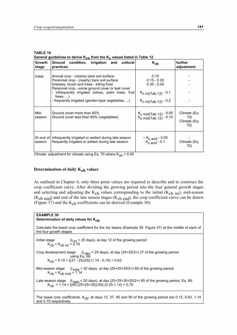
Crop evapotranspiration
141
TABLE 18 General guidelines to derive Kcb from the Kc values listed in Table 12 Growth stage
Ground condition, irrigation and cultural practices
Kcb further adjustment
Initial
Annual crop - (nearly) bare soil surface Perennial crop - (nearly) bare soil surface Grasses, brush and trees - killing frost Perennial crop - some ground cover or leaf cover - infrequently irrigated (olives, palm trees, fruit
trees, ...) - frequently irrigated (garden-type vegetables, ...)
0.15
0.15 - 0.20 0.30 - 0.40
Kc ini(Tab.12) - 0.1
Kc ini(Tab.12) - 0.2
- - - - -
Mid-season
Ground cover more than 80% Ground cover less than 80% (vegetables)
Kc mid(Tab.12) - 0.05 Kc mid(Tab.12) - 0.10
Climate (Eq.
70) Climate (Eq.
70)
At end of season
infrequently irrigated or wetted during late season frequently irrigated or wetted during late season
~ Kc end - 0.05
Kc end - 0.1
-
Climate (Eq. 70)
Climate: adjustment for climate using Eq. 70 where Kcb > 0.45 Determination of daily Kcb values
As outlined in Chapter 6, only three point values are required to describe and to construct the crop coefficient curve. After dividing the growing period into the four general growth stages and selecting and adjusting the Kcb values corresponding to the initial (Kcb ini), mid-season (Kcb mid) and end of the late season stages (Kcb end), the crop coefficient curve can be drawn (Figure 37) and the Kcb coefficients can be derived (Example 30).
EXAMPLE 30 Determination of daily values for Kcb Calculate the basal crop coefficient for the dry beans (Example 29, Figure 37) at the middle of each of the four growth stages. Initial stage (Lini = 25 days), at day 12 of the growing period: Kcb = Kcb ini = 0.15 Crop development stage (Ldev = 25 days), at day (25+25/2=) 37 of the growing period, using Eq. 66: Kcb = 0.15 + [(37 - 25)/25] (1.14 - 0.15) = 0.63 Mid-season stage (Lmid = 30 days), at day (25+25+30/2=) 65 of the growing period: Kcb = Kcb mid = 1.14 Late season stage (Llate = 20 days), at day (25+25+30+20/2=) 90 of the growing period, Eq. 66: Kcb = 1.14 + [(90-(25+25+30))/20] (0.25-1.14) = 0.70 The basal crop coefficients, Kcb, at days 12, 37, 65 and 90 of the growing period are 0.15, 0.63, 1.14 and 0.70 respectively.
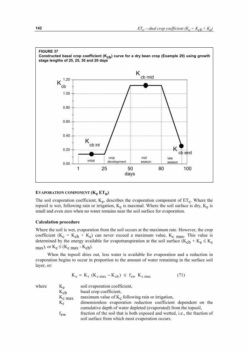
ETc -–dual crop coefficient (Kc = Kcb + Ke)
142
EVAPORATION COMPONENT (Ke ETo)
The soil evaporation coefficient, Ke, describes the evaporation component of ETc. Where the topsoil is wet, following rain or irrigation, Ke is maximal. Where the soil surface is dry, Ke is small and even zero when no water remains near the soil surface for evaporation. Calculation procedure
Where the soil is wet, evaporation from the soil occurs at the maximum rate. However, the crop coefficient (Kc = Kcb + Ke) can never exceed a maximum value, Kc max. This value is determined by the energy available for evapotranspiration at the soil surface (Kcb + Ke ≤ Kc max), or Ke ≤ (Kc max - Kcb).
When the topsoil dries out, less water is available for evaporation and a reduction in evaporation begins to occur in proportion to the amount of water remaining in the surface soil layer, or:
maxcewcbmaxcre Kf)KK(KK ≤−= (71) where Ke soil evaporation coefficient,
Kcb basal crop coefficient, Kc max maximum value of Kc following rain or irrigation, Kr dimensionless evaporation reduction coefficient dependent on the
cumulative depth of water depleted (evaporated) from the topsoil, few fraction of the soil that is both exposed and wetted, i.e., the fraction of
soil surface from which most evaporation occurs.
FIGURE 37 Constructed basal crop coefficient (Kcb) curve for a dry bean crop (Example 29) using growth stage lengths of 25, 25, 30 and 20 days
0.00
0.20
0.40
0.60
0.80
1.00
1.20
KK
initial cropdevelopment
midseason
lateseason
Kcb
cb ini
Kcb mid
cb end
1 25 50 80 100days
Crop evapotranspiration
143
In computer programming terminology, Equation 71 is expressed as Ke = min(Kr (Kc max - Kcb), few Kc max).
Following rain or irrigation Kr is 1, and evaporation is only determined by the energy available for evaporation. As the soil surface dries, Kr becomes less than one and evaporation is reduced. Kr becomes zero when no water is left for evaporation in the upper soil layer.
Evaporation occurs predominantly from the exposed soil fraction. Hence, evaporation is restricted at any moment by the energy available at the exposed soil fraction, i.e., Ke cannot exceed few Kc max, where few is the fraction of soil from which most evaporation occurs, i.e., the fraction of the soil not covered by vegetation and that is wetted by irrigation or precipitation.
The calculation procedure consists in determining: • the upper limit Kc max; • the soil evaporation reduction coefficient Kr; and • the exposed and wetted soil fraction few.
The estimation of Kr requires a daily water balance computation for the surface soil layer. Upper limit Kc max Kc max represents an upper limit on the evaporation and transpiration from any cropped surface and is imposed to reflect the natural constraints placed on available energy represented by the energy balance difference Rn - G - H (Equation 1). Kc max ranges from about 1.05 to 1.30 when using the grass reference ETo:
[ ] { }��
�
�
��
�
�+
��
�
��
��
��
���
�−−−+= 05.0K,3h)45RH(004.0)2u(04.02.1maxK cb
3.0
min2maxc (72)
where h mean maximum plant height during the period of calculation (initial,
development, mid-season, or late-season) [m], Kcb basal crop coefficient, max ( ) maximum value of the parameters in braces { } that are separated by
the comma.
Equation 72 ensures that Kc max is always greater or equal to the sum Kcb + 0.05. This requirement suggests that wet soil will always increase the value for Kcb by 0.05 following complete wetting of the soil surface, even during periods of full ground cover. A value of 1.2 instead of 1 is used for Kc max in Equation 72 because of the effect of increased aerodynamic roughness of surrounding crops during development, mid-season and late season growth stages which can increase the turbulent transfer of vapour from the exposed soil surface. The “1.2” coefficient also reflects the impact of the reduced albedo of wet soil and the contribution of heat stored in dry soil prior to the wetting event. All of these factors can contribute to increased evaporation relative to the reference.
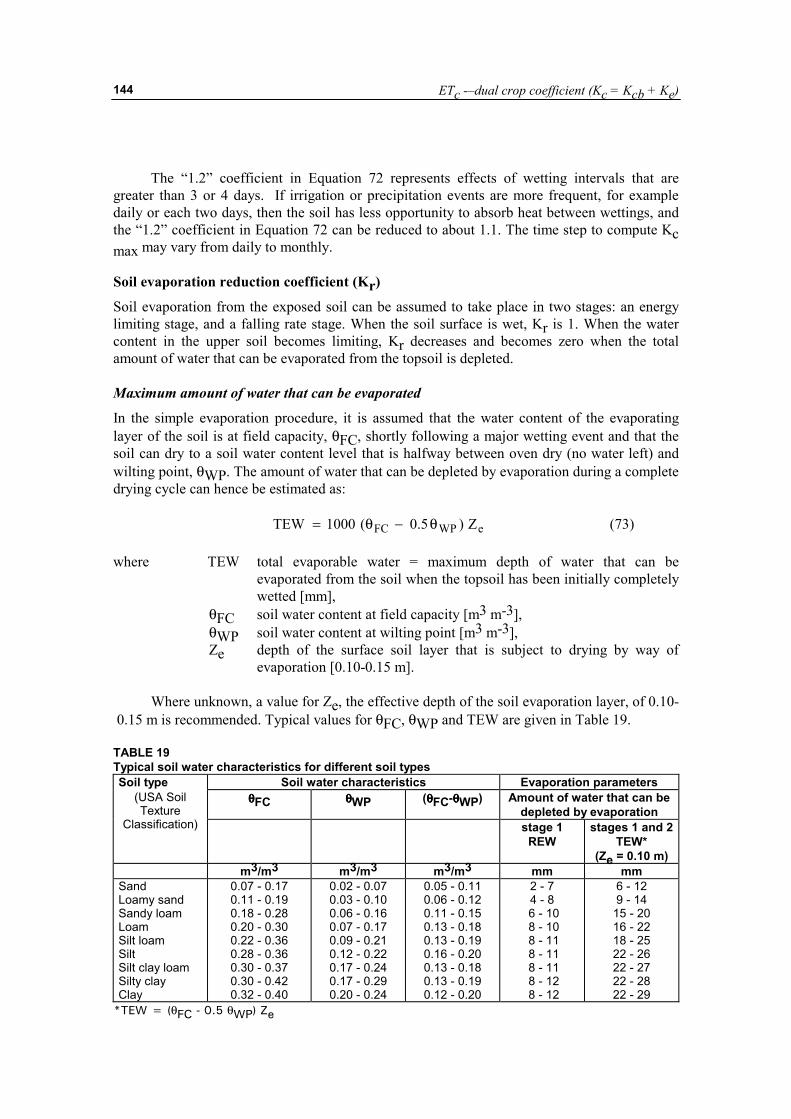
ETc -–dual crop coefficient (Kc = Kcb + Ke)
144
The “1.2” coefficient in Equation 72 represents effects of wetting intervals that are greater than 3 or 4 days. If irrigation or precipitation events are more frequent, for example daily or each two days, then the soil has less opportunity to absorb heat between wettings, and the “1.2” coefficient in Equation 72 can be reduced to about 1.1. The time step to compute Kc max may vary from daily to monthly. Soil evaporation reduction coefficient (Kr)
Soil evaporation from the exposed soil can be assumed to take place in two stages: an energy limiting stage, and a falling rate stage. When the soil surface is wet, Kr is 1. When the water content in the upper soil becomes limiting, Kr decreases and becomes zero when the total amount of water that can be evaporated from the topsoil is depleted. Maximum amount of water that can be evaporated
In the simple evaporation procedure, it is assumed that the water content of the evaporating layer of the soil is at field capacity, θFC, shortly following a major wetting event and that the soil can dry to a soil water content level that is halfway between oven dry (no water left) and wilting point, θWP. The amount of water that can be depleted by evaporation during a complete drying cycle can hence be estimated as:
eWPFC Z)5.0(1000TEW θ−θ= (73) where TEW total evaporable water = maximum depth of water that can be
evaporated from the soil when the topsoil has been initially completely wetted [mm],
θFC soil water content at field capacity [m3 m-3], θWP soil water content at wilting point [m3 m-3], Ze depth of the surface soil layer that is subject to drying by way of
evaporation [0.10-0.15 m]. Where unknown, a value for Ze, the effective depth of the soil evaporation layer, of 0.10- 0.15 m is recommended. Typical values for θFC, θWP and TEW are given in Table 19. TABLE 19 Typical soil water characteristics for different soil types Soil type Soil water characteristics Evaporation parameters
θθθθFC θθθθWP (θθθθFC-θθθθWP) Amount of water that can be depleted by evaporation
(USA Soil Texture
Classification) stage 1 REW
stages 1 and 2TEW*
(Ze = 0.10 m) m3/m3 m3/m3 m3/m3 mm mm Sand Loamy sand Sandy loam Loam Silt loam Silt Silt clay loam Silty clay Clay
0.07 - 0.17 0.11 - 0.19 0.18 - 0.28 0.20 - 0.30 0.22 - 0.36 0.28 - 0.36 0.30 - 0.37 0.30 - 0.42 0.32 - 0.40
0.02 - 0.07 0.03 - 0.10 0.06 - 0.16 0.07 - 0.17 0.09 - 0.21 0.12 - 0.22 0.17 - 0.24 0.17 - 0.29 0.20 - 0.24
0.05 - 0.11 0.06 - 0.12 0.11 - 0.15 0.13 - 0.18 0.13 - 0.19 0.16 - 0.20 0.13 - 0.18 0.13 - 0.19 0.12 - 0.20
2 - 7 4 - 8
6 - 10 8 - 10 8 - 11 8 - 11 8 - 11 8 - 12 8 - 12
6 - 12 9 - 14
15 - 20 16 - 22 18 - 25 22 - 26 22 - 27 22 - 28 22 - 29
*TEW = (θFC - 0.5 θWP) Ze
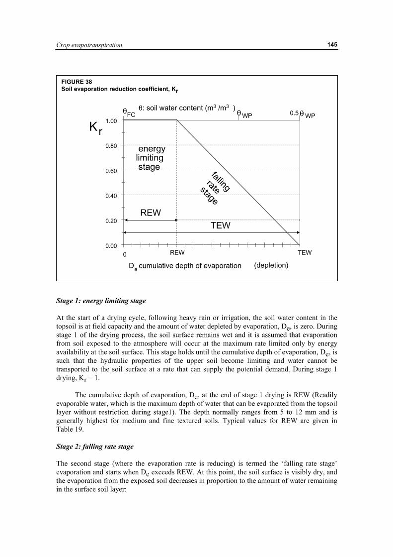
Crop evapotranspiration
145
Stage 1: energy limiting stage At the start of a drying cycle, following heavy rain or irrigation, the soil water content in the topsoil is at field capacity and the amount of water depleted by evaporation, De, is zero. During stage 1 of the drying process, the soil surface remains wet and it is assumed that evaporation from soil exposed to the atmosphere will occur at the maximum rate limited only by energy availability at the soil surface. This stage holds until the cumulative depth of evaporation, De, is such that the hydraulic properties of the upper soil become limiting and water cannot be transported to the soil surface at a rate that can supply the potential demand. During stage 1 drying, Kr = 1.
The cumulative depth of evaporation, De, at the end of stage 1 drying is REW (Readily evaporable water, which is the maximum depth of water that can be evaporated from the topsoil layer without restriction during stage1). The depth normally ranges from 5 to 12 mm and is generally highest for medium and fine textured soils. Typical values for REW are given in Table 19. Stage 2: falling rate stage The second stage (where the evaporation rate is reducing) is termed the ‘falling rate stage’ evaporation and starts when De exceeds REW. At this point, the soil surface is visibly dry, and the evaporation from the exposed soil decreases in proportion to the amount of water remaining in the surface soil layer:
FIGURE 38 Soil evaporation reduction coefficient, Kr
energylimiting stage falling
rate stage
θFC WP WP0.5
Kr
(depletion)0 TEWREW
REWTEW
θ: soil water content (m3 /m3 )
D cumulative depth of evaporatione
0.00
0.20
0.40
0.60
0.80
1.00θ θ
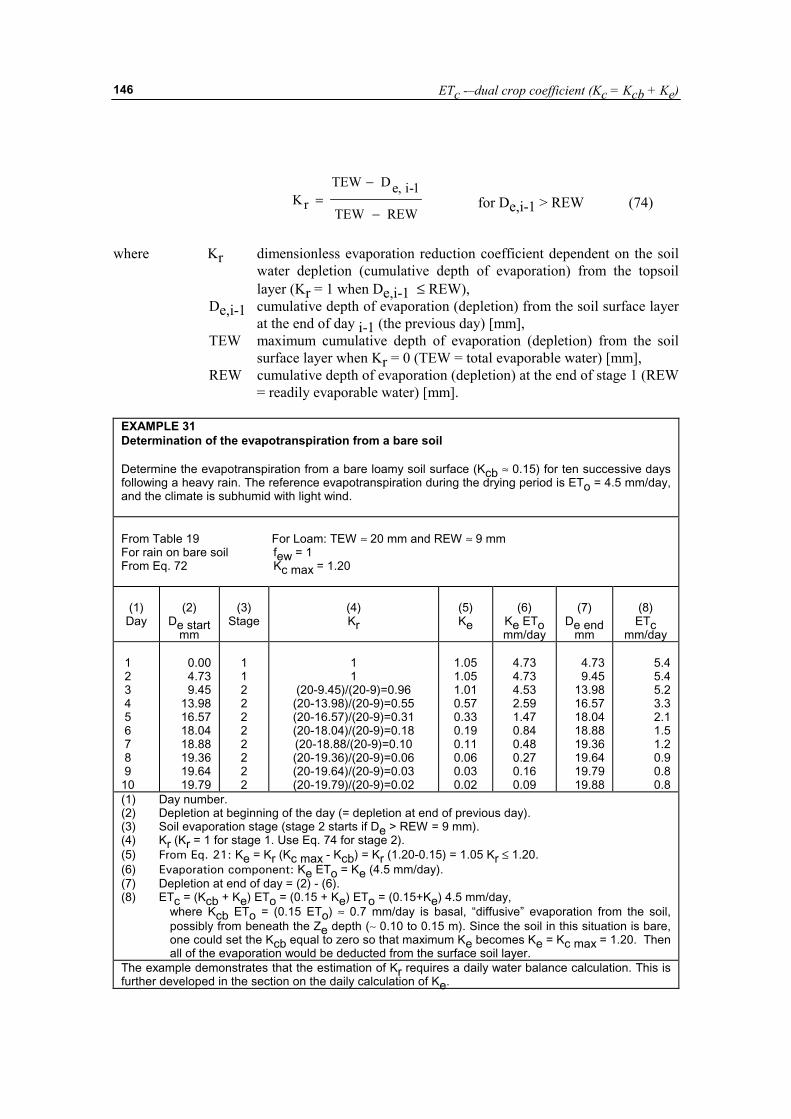
ETc -–dual crop coefficient (Kc = Kcb + Ke)
146
REWTEW
1-i,eDTEWrK
−
−= for De,i-1 > REW (74)
where Kr dimensionless evaporation reduction coefficient dependent on the soil
water depletion (cumulative depth of evaporation) from the topsoil layer (Kr = 1 when De,i-1 ≤ REW),
De,i-1 cumulative depth of evaporation (depletion) from the soil surface layer at the end of day i-1 (the previous day) [mm],
TEW maximum cumulative depth of evaporation (depletion) from the soil surface layer when Kr = 0 (TEW = total evaporable water) [mm],
REW cumulative depth of evaporation (depletion) at the end of stage 1 (REW = readily evaporable water) [mm].
EXAMPLE 31 Determination of the evapotranspiration from a bare soil Determine the evapotranspiration from a bare loamy soil surface (Kcb ≈ 0.15) for ten successive days following a heavy rain. The reference evapotranspiration during the drying period is ETo = 4.5 mm/day, and the climate is subhumid with light wind. From Table 19 For Loam: TEW ≈ 20 mm and REW ≈ 9 mm For rain on bare soil few = 1 From Eq. 72 Kc max = 1.20
(1) Day
(2)
De start mm
(3)
Stage
(4) Kr
(5) Ke
(6)
Ke ETo mm/day
(7)
De end mm
(8) ETc
mm/day 1 2 3 4 5 6 7 8 9 10
0.00 4.73 9.45
13.98 16.57 18.04 18.88 19.36 19.64 19.79
1 1 2 2 2 2 2 2 2 2
1 1
(20-9.45)/(20-9)=0.96 (20-13.98)/(20-9)=0.55 (20-16.57)/(20-9)=0.31 (20-18.04)/(20-9)=0.18 (20-18.88/(20-9)=0.10 (20-19.36)/(20-9)=0.06 (20-19.64)/(20-9)=0.03 (20-19.79)/(20-9)=0.02
1.05 1.05 1.01 0.57 0.33 0.19 0.11 0.06 0.03 0.02
4.73 4.73 4.53 2.59 1.47 0.84 0.48 0.27 0.16 0.09
4.73 9.45
13.98 16.57 18.04 18.88 19.36 19.64 19.79 19.88
5.4 5.4 5.2 3.3 2.1 1.5 1.2 0.9 0.8 0.8
(1) Day number. (2) Depletion at beginning of the day (= depletion at end of previous day). (3) Soil evaporation stage (stage 2 starts if De > REW = 9 mm). (4) Kr (Kr = 1 for stage 1. Use Eq. 74 for stage 2). (5) From Eq. 21: Ke = Kr (Kc max - Kcb) = Kr (1.20-0.15) = 1.05 Kr ≤ 1.20. (6) Evaporation component: Ke ETo = Ke (4.5 mm/day). (7) Depletion at end of day = (2) - (6). (8) ETc = (Kcb + Ke) ETo = (0.15 + Ke) ETo = (0.15+Ke) 4.5 mm/day, where Kcb ETo = (0.15 ETo) ≈ 0.7 mm/day is basal, “diffusive” evaporation from the soil,
possibly from beneath the Ze depth (∼ 0.10 to 0.15 m). Since the soil in this situation is bare, one could set the Kcb equal to zero so that maximum Ke becomes Ke = Kc max = 1.20. Then all of the evaporation would be deducted from the surface soil layer.
The example demonstrates that the estimation of Kr requires a daily water balance calculation. This is further developed in the section on the daily calculation of Ke.
Crop evapotranspiration
147
Exposed and wetted soil fraction (few)
few: calculation procedure
In crops with incomplete ground cover, evaporation from the soil often does not occur uniformly over the entire surface, but is greater between plants where exposure to sunlight occurs and where more air ventilation is able to transport vapour from the soil surface to above the canopy. This is especially true where only part of the soil surface is wetted by irrigation.
It is recognized that both the location and the fraction of the soil surface exposed to sunlight change to some degree with the time of day and depending on row orientation. The procedure presented here predicts a general averaged fraction of the soil surface from which the majority of evaporation occurs. Diffusive evaporation from the soil beneath the crop canopy is assumed to be largely included in the basal Kcb coefficient.
Where the complete soil surface is wetted, as by precipitation or sprinkler, then the fraction of soil surface from which most evaporation occurs, few, is essentially defined as (1-fc), where fc is the average fraction of soil surface covered by vegetation and (1-fc) is the approximate fraction of soil surface that is exposed. However, for irrigation systems where only a fraction of the ground surface is wetted, few must be limited to fw, the fraction of the soil surface wetted by irrigation (Figure 39). Therefore, few is calculated as:
( )wcew f,f1minf −= (75) where 1-fc average exposed soil fraction not covered (or shaded) by vegetation [0.01 - 1], fw average fraction of soil surface wetted by irrigation or precipitation [0.01 - 1].
The ‘min()’ function selects the lowest value of the ‘1-fc’ and ‘fw’ values. Figure 39 illustrates the relation of few to (1-fc) and fw.
The limitation imposed by Equation 75 assumes that the fraction of soil wetted by irrigation occurs within the fraction of soil exposed to sunlight and ventilation. This is generally the case, except perhaps with drip irrigation (Figure 39).
In the case of drip irrigation, where the majority of soil wetted by irrigation may be beneath the canopy and may therefore be shaded, more complex models of the soil surface and wetting patterns may be required to accurately estimate total evaporation from the soil. In this case, the value for fw may need to be reduced to about one-half to one-third of that given in Table 20 to account for the effects of shading of emitters by the plant canopy on the evaporation rate from wetted soil (Example 34). A general approach could be to multiply fw by [1-(2/3)fc] for drip irrigation. fw: fraction of soil surface wetted by irrigation or precipitation
Table 20 presents typical values for fw. Where a mixture of irrigation and precipitation occur within the same drying period or on the same day, the value for fw should be based on a weighted average of the fw for precipitation (fw = 1) and the fw for the irrigation system. The weighting should be approximately proportional to the infiltration depths from each water source.
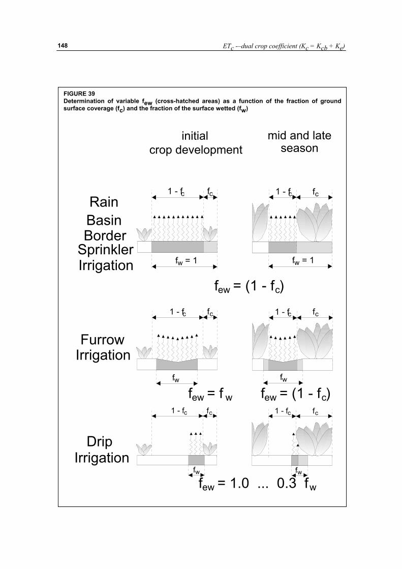
ETc -–dual crop coefficient (Kc = Kcb + Ke)
148
FIGURE 39 Determination of variable few (cross-hatched areas) as a function of the fraction of ground surface coverage (fc) and the fraction of the surface wetted (fw)
initialcrop development
mid and late season
few = (1 - f c)
RainBasinBorder
SprinklerIrrigation
1 - f fc c
f = 1w f = 1w
1 - f fc c
few = f w few = (1 - f c)
few = 1.0 ... 0.3 f w
FurrowIrrigation
DripIrrigation
1 - fc 1 - fc
1 - fc 1 - fc fcfc
fc fc
fw fw
fwfw
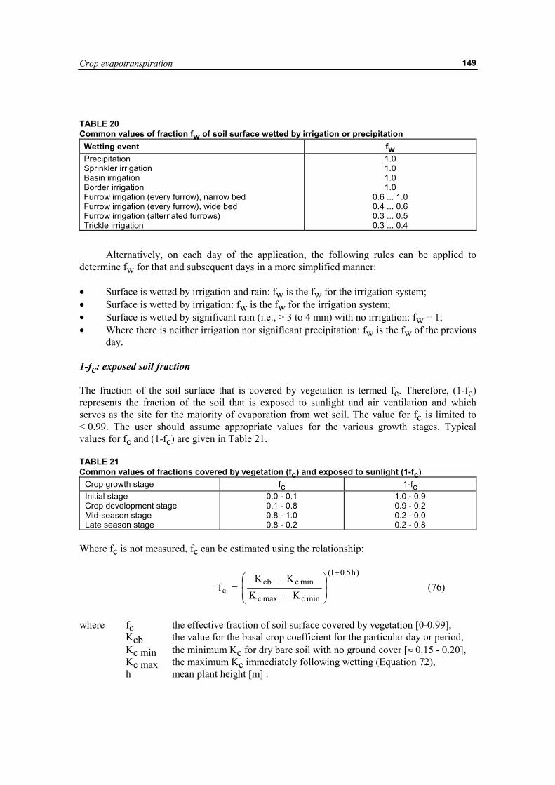
Crop evapotranspiration
149
TABLE 20 Common values of fraction fw of soil surface wetted by irrigation or precipitation Wetting event fw Precipitation Sprinkler irrigation Basin irrigation Border irrigation Furrow irrigation (every furrow), narrow bed Furrow irrigation (every furrow), wide bed Furrow irrigation (alternated furrows) Trickle irrigation
1.0 1.0 1.0 1.0
0.6 ... 1.0 0.4 ... 0.6 0.3 ... 0.5 0.3 ... 0.4
Alternatively, on each day of the application, the following rules can be applied to
determine fw for that and subsequent days in a more simplified manner: • Surface is wetted by irrigation and rain: fw is the fw for the irrigation system; • Surface is wetted by irrigation: fw is the fw for the irrigation system; • Surface is wetted by significant rain (i.e., > 3 to 4 mm) with no irrigation: fw = 1; • Where there is neither irrigation nor significant precipitation: fw is the fw of the previous
day. 1-fc: exposed soil fraction The fraction of the soil surface that is covered by vegetation is termed fc. Therefore, (1-fc) represents the fraction of the soil that is exposed to sunlight and air ventilation and which serves as the site for the majority of evaporation from wet soil. The value for fc is limited to < 0.99. The user should assume appropriate values for the various growth stages. Typical values for fc and (1-fc) are given in Table 21. TABLE 21 Common values of fractions covered by vegetation (fc) and exposed to sunlight (1-fc)
Crop growth stage fc 1-fc Initial stage Crop development stage Mid-season stage Late season stage
0.0 - 0.1 0.1 - 0.8 0.8 - 1.0 0.8 - 0.2
1.0 - 0.9 0.9 - 0.2 0.2 - 0.0 0.2 - 0.8
Where fc is not measured, fc can be estimated using the relationship:
)h5.01(
mincmaxc
mincbcc KK
KKf
+
��
�
�
��
�
�
−
−= (76)
where fc the effective fraction of soil surface covered by vegetation [0-0.99],
Kcb the value for the basal crop coefficient for the particular day or period, Kc min the minimum Kc for dry bare soil with no ground cover [≈ 0.15 - 0.20], Kc max the maximum Kc immediately following wetting (Equation 72), h mean plant height [m] .
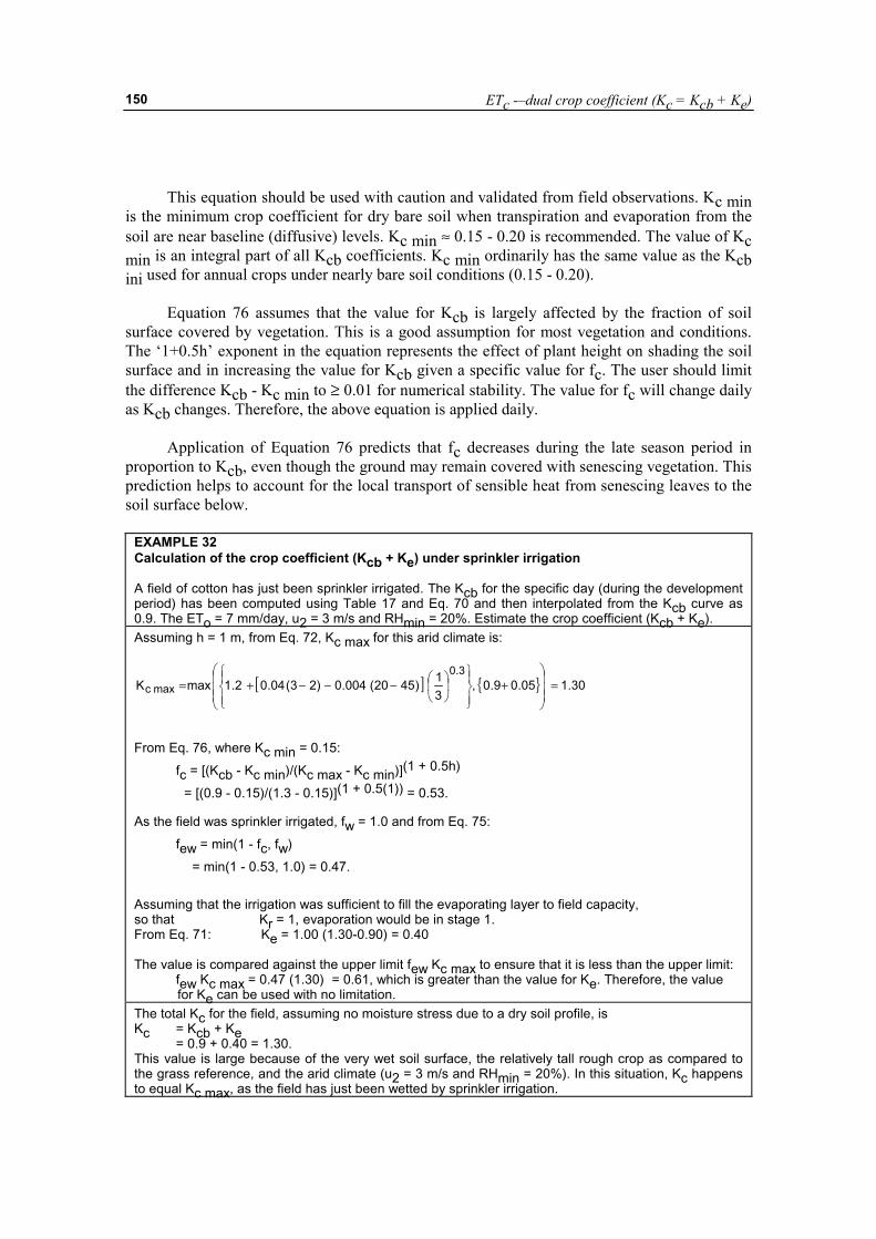
ETc -–dual crop coefficient (Kc = Kcb + Ke)
150
This equation should be used with caution and validated from field observations. Kc min is the minimum crop coefficient for dry bare soil when transpiration and evaporation from the soil are near baseline (diffusive) levels. Kc min ≈ 0.15 - 0.20 is recommended. The value of Kc min is an integral part of all Kcb coefficients. Kc min ordinarily has the same value as the Kcb ini used for annual crops under nearly bare soil conditions (0.15 - 0.20).
Equation 76 assumes that the value for Kcb is largely affected by the fraction of soil surface covered by vegetation. This is a good assumption for most vegetation and conditions. The ‘1+0.5h’ exponent in the equation represents the effect of plant height on shading the soil surface and in increasing the value for Kcb given a specific value for fc. The user should limit the difference Kcb - Kc min to ≥ 0.01 for numerical stability. The value for fc will change daily as Kcb changes. Therefore, the above equation is applied daily.
Application of Equation 76 predicts that fc decreases during the late season period in proportion to Kcb, even though the ground may remain covered with senescing vegetation. This prediction helps to account for the local transport of sensible heat from senescing leaves to the soil surface below.
EXAMPLE 32 Calculation of the crop coefficient (Kcb + Ke) under sprinkler irrigation A field of cotton has just been sprinkler irrigated. The Kcb for the specific day (during the development period) has been computed using Table 17 and Eq. 70 and then interpolated from the Kcb curve as 0.9. The ETo = 7 mm/day, u2 = 3 m/s and RHmin = 20%. Estimate the crop coefficient (Kcb + Ke). Assuming h = 1 m, from Eq. 72, Kc max for this arid climate is:
[ ] { } 30.105.09.0,31)4520(004.0)23(04.02.1maxK
3.0maxc =
���
�
�
���
�
�+
��
�
��
��
��
���
�−−−+=
From Eq. 76, where Kc min = 0.15:
fc = [(Kcb - Kc min)/(Kc max - Kc min)](1 + 0.5h)
= [(0.9 - 0.15)/(1.3 - 0.15)](1 + 0.5(1)) = 0.53.
As the field was sprinkler irrigated, fw = 1.0 and from Eq. 75:
few = min(1 - fc, fw)
= min(1 - 0.53, 1.0) = 0.47.
Assuming that the irrigation was sufficient to fill the evaporating layer to field capacity, so that Kr = 1, evaporation would be in stage 1. From Eq. 71: Ke = 1.00 (1.30-0.90) = 0.40 The value is compared against the upper limit few Kc max to ensure that it is less than the upper limit: few Kc max = 0.47 (1.30) = 0.61, which is greater than the value for Ke. Therefore, the value
for Ke can be used with no limitation. The total Kc for the field, assuming no moisture stress due to a dry soil profile, is Kc = Kcb + Ke = 0.9 + 0.40 = 1.30. This value is large because of the very wet soil surface, the relatively tall rough crop as compared to the grass reference, and the arid climate (u2 = 3 m/s and RHmin = 20%). In this situation, Kc happens to equal Kc max, as the field has just been wetted by sprinkler irrigation.
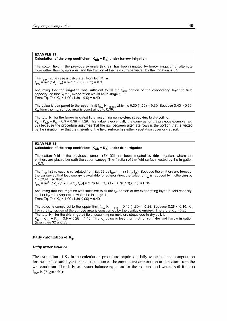
Crop evapotranspiration
151
EXAMPLE 33 Calculation of the crop coefficient (Kcb + Ke) under furrow irrigation The cotton field in the previous example (Ex. 32) has been irrigated by furrow irrigation of alternate rows rather than by sprinkler, and the fraction of the field surface wetted by the irrigation is 0.3. The few in this case is calculated from Eq. 75 as: few = min(1-fc, fw) = min(1 - 0.53, 0.3) = 0.3. Assuming that the irrigation was sufficient to fill the few portion of the evaporating layer to field capacity, so that Kr = 1, evaporation would be in stage 1. From Eq. 71: Ke = 1.00 (1.30 - 0.9) = 0.40 The value is compared to the upper limit few Kc max which is 0.30 (1.30) = 0.39. Because 0.40 > 0.39, Ke from the few surface area is constrained to 0.39. The total Kc for the furrow irrigated field, assuming no moisture stress due to dry soil, is Kc = Kcb + Ke = 0.9 + 0.39 = 1.29. This value is essentially the same as for the previous example (Ex. 32) because the procedure assumes that the soil between alternate rows is the portion that is wetted by the irrigation, so that the majority of the field surface has either vegetation cover or wet soil.
EXAMPLE 34 Calculation of the crop coefficient (Kcb + Ke) under drip irrigation The cotton field in the previous example (Ex. 32) has been irrigated by drip irrigation, where the emitters are placed beneath the cotton canopy. The fraction of the field surface wetted by the irrigation is 0.3. The few in this case is calculated from Eq. 75 as few = min(1-fc, fw). Because the emitters are beneath the canopy so that less energy is available for evaporation, the value for fw is reduced by multiplying by 1 - (2/3)fc, so that: few = min[(1-fc),(1 - 0.67 fc) fw)] = min[(1-0.53), (1 - 0.67(0.53))(0.3)] = 0.19 Assuming that the irrigation was sufficient to fill the fw portion of the evaporating layer to field capacity, so that Kr = 1, evaporation would be in stage 1. From Eq. 71: Ke = 1.00 (1.30-0.90) = 0.40. The value is compared to the upper limit few Kc max = 0.19 (1.30) = 0.25. Because 0.25 < 0.40, Ke from the fw fraction of the surface area is constrained by the available energy. Therefore Ke = 0.25. The total Kc for the drip irrigated field, assuming no moisture stress due to dry soil, is: Kc = Kcb + Ke = 0.9 + 0.25 = 1.15. This Kc value is less than that for sprinkler and furrow irrigation (Examples 32 and 33).
Daily calculation of Ke Daily water balance The estimation of Ke in the calculation procedure requires a daily water balance computation for the surface soil layer for the calculation of the cumulative evaporation or depletion from the wet condition. The daily soil water balance equation for the exposed and wetted soil fraction few is (Figure 40):
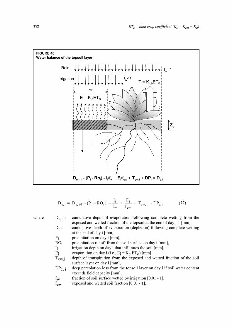
ETc -–dual crop coefficient (Kc = Kcb + Ke)
152
i e,i,ewew
i
w
iii1-i,ei,e DPT
fE
+fI
)RO(PDD ++−−−= (77)
where De,i-1 cumulative depth of evaporation following complete wetting from the
exposed and wetted fraction of the topsoil at the end of day i-1 [mm], De,i cumulative depth of evaporation (depletion) following complete wetting
at the end of day i [mm], Pi precipitation on day i [mm], ROi precipitation runoff from the soil surface on day i [mm], Ii irrigation depth on day i that infiltrates the soil [mm], Ei evaporation on day i (i.e., Ei = Ke ETo) [mm], Tew,i depth of transpiration from the exposed and wetted fraction of the soil
surface layer on day i [mm], DPe, i deep percolation loss from the topsoil layer on day i if soil water content
exceeds field capacity [mm], fw fraction of soil surface wetted by irrigation [0.01 - 1], few exposed and wetted soil fraction [0.01 - 1].
FIGURE 40 Water balance of the topsoil layer
f < 1Irrigation
Rain
few
T = K ET
E = K ET
cb
e o
ow
Ze
fw=1
De,I-1 - (Pi - Roi) - Ii/fw + Ei/few + Tew,i + DPi = De,i
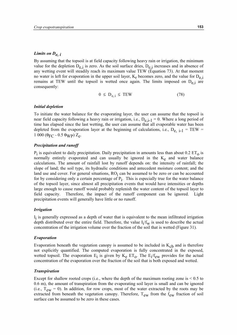
Crop evapotranspiration
153
Limits on De, i
By assuming that the topsoil is at field capacity following heavy rain or irrigation, the minimum value for the depletion De,i is zero. As the soil surface dries, De,i increases and in absence of any wetting event will steadily reach its maximum value TEW (Equation 73). At that moment no water is left for evaporation in the upper soil layer, Kr becomes zero, and the value for De,i remains at TEW until the topsoil is wetted once again. The limits imposed on De,i are consequently:
TEWD0 i,e ≤≤ (78) Initial depletion
To initiate the water balance for the evaporating layer, the user can assume that the topsoil is near field capacity following a heavy rain or irrigation, i.e., De,i-1 = 0. Where a long period of time has elapsed since the last wetting, the user can assume that all evaporable water has been depleted from the evaporation layer at the beginning of calculations, i.e., De, i-1 = TEW = 1 000 (θFC - 0.5 θWP) Ze. Precipitation and runoff
Pi is equivalent to daily precipitation. Daily precipitation in amounts less than about 0.2 ETo is normally entirely evaporated and can usually be ignored in the Ke and water balance calculations. The amount of rainfall lost by runoff depends on: the intensity of rainfall; the slope of land; the soil type, its hydraulic conditions and antecedent moisture content; and the land use and cover. For general situations, ROi can be assumed to be zero or can be accounted for by considering only a certain percentage of Pi. This is especially true for the water balance of the topsoil layer, since almost all precipitation events that would have intensities or depths large enough to cause runoff would probably replenish the water content of the topsoil layer to field capacity. Therefore, the impact of the runoff component can be ignored. Light precipitation events will generally have little or no runoff. Irrigation
Ii is generally expressed as a depth of water that is equivalent to the mean infiltrated irrigation depth distributed over the entire field. Therefore, the value Ii/fw is used to describe the actual concentration of the irrigation volume over the fraction of the soil that is wetted (Figure 31). Evaporation
Evaporation beneath the vegetation canopy is assumed to be included in Kcb and is therefore not explicitly quantified. The computed evaporation is fully concentrated in the exposed, wetted topsoil. The evaporation Ei is given by Ke ETo. The Ei/few provides for the actual concentration of the evaporation over the fraction of the soil that is both exposed and wetted. Transpiration
Except for shallow rooted crops (i.e., where the depth of the maximum rooting zone is < 0.5 to 0.6 m), the amount of transpiration from the evaporating soil layer is small and can be ignored (i.e., Tew = 0). In addition, for row crops, most of the water extracted by the roots may be extracted from beneath the vegetation canopy. Therefore, Tew from the few fraction of soil surface can be assumed to be zero in these cases.
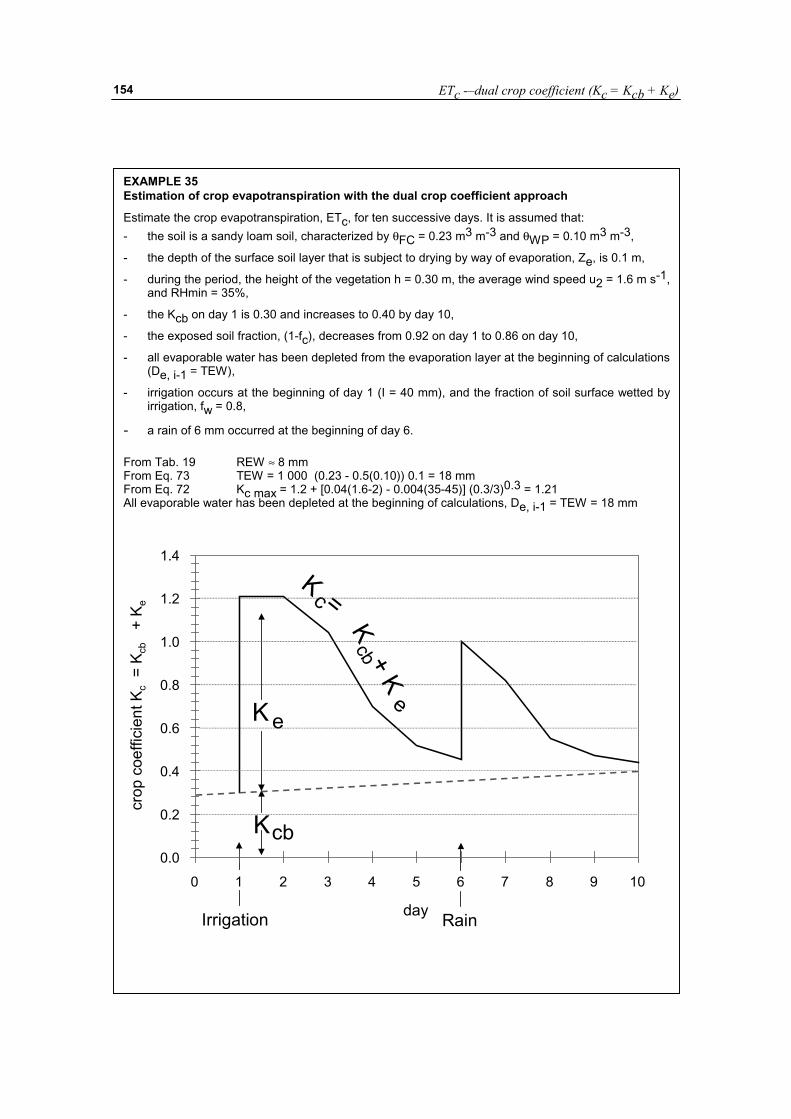
ETc -–dual crop coefficient (Kc = Kcb + Ke)
154
EXAMPLE 35 Estimation of crop evapotranspiration with the dual crop coefficient approach
Estimate the crop evapotranspiration, ETc, for ten successive days. It is assumed that: - the soil is a sandy loam soil, characterized by θFC = 0.23 m3 m-3 and θWP = 0.10 m3 m-3,
- the depth of the surface soil layer that is subject to drying by way of evaporation, Ze, is 0.1 m,
- during the period, the height of the vegetation h = 0.30 m, the average wind speed u2 = 1.6 m s-1, and RHmin = 35%,
- the Kcb on day 1 is 0.30 and increases to 0.40 by day 10,
- the exposed soil fraction, (1-fc), decreases from 0.92 on day 1 to 0.86 on day 10,
- all evaporable water has been depleted from the evaporation layer at the beginning of calculations(De, i-1 = TEW),
- irrigation occurs at the beginning of day 1 (I = 40 mm), and the fraction of soil surface wetted byirrigation, fw = 0.8,
- a rain of 6 mm occurred at the beginning of day 6. From Tab. 19 REW ≈ 8 mm From Eq. 73 TEW = 1 000 (0.23 - 0.5(0.10)) 0.1 = 18 mm From Eq. 72 Kc max = 1.2 + [0.04(1.6-2) - 0.004(35-45)] (0.3/3)0.3 = 1.21 All evaporable water has been depleted at the beginning of calculations, De, i-1 = TEW = 18 mm
K
K
e
cb
Irrigation Rain
K =c
cb
e
K + K
0.0
0.2
0.4
0.6
0.8
1.0
1.2
1.4
0 1 2 3 4 5 6 7 8 9 10
day
crop
coe
ffici
ent K
c =
K cb
+ K
e
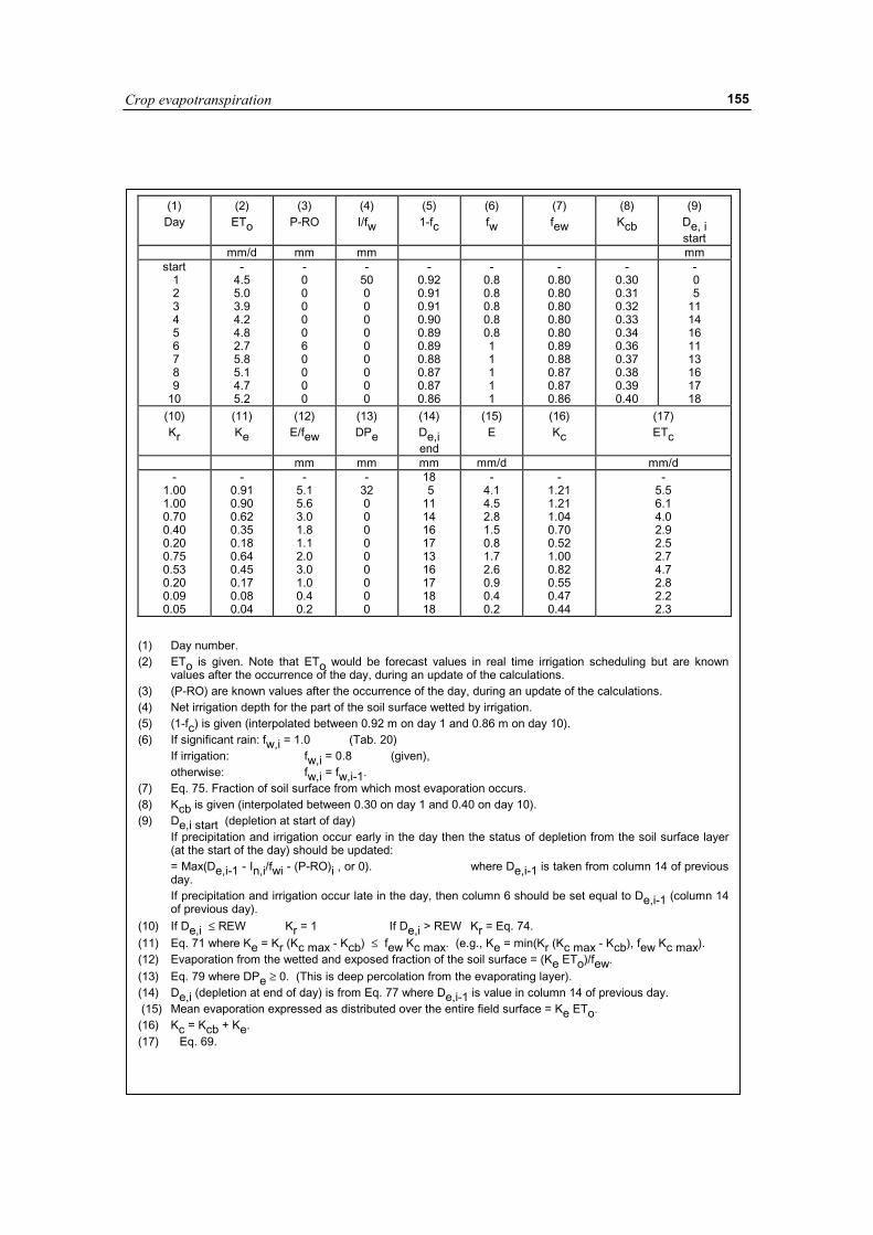
Crop evapotranspiration
155
(1) Day
(2) ETo
(3) P-RO
(4) I/fw
(5) 1-fc
(6) fw
(7) few
(8) Kcb
(9) De, i start
mm/d mm mm mm start
1 2 3 4 5 6 7 8 9 10
- 4.5 5.0 3.9 4.2 4.8 2.7 5.8 5.1 4.7 5.2
- 0 0 0 0 0 6 0 0 0 0
- 50 0 0 0 0 0 0 0 0 0
- 0.92 0.91 0.91 0.90 0.89 0.89 0.88 0.87 0.87 0.86
- 0.8 0.8 0.8 0.8 0.8 1 1 1 1 1
- 0.80 0.80 0.80 0.80 0.80 0.89 0.88 0.87 0.87 0.86
- 0.30 0.31 0.32 0.33 0.34 0.36 0.37 0.38 0.39 0.40
- 0 5 11 14 16 11 13 16 17 18
(10) Kr
(11) Ke
(12) E/few
(13) DPe
(14) De,i end
(15) E
(16) Kc
(17) ETc
mm mm mm mm/d mm/d -
1.00 1.00 0.70 0.40 0.20 0.75 0.53 0.20 0.09 0.05
- 0.91 0.90 0.62 0.35 0.18 0.64 0.45 0.17 0.08 0.04
- 5.1 5.6 3.0 1.8 1.1 2.0 3.0 1.0 0.4 0.2
- 32 0 0 0 0 0 0 0 0 0
18 5 11 14 16 17 13 16 17 18 18
- 4.1 4.5 2.8 1.5 0.8 1.7 2.6 0.9 0.4 0.2
- 1.21 1.21 1.04 0.70 0.52 1.00 0.82 0.55 0.47 0.44
- 5.5 6.1 4.0 2.9 2.5 2.7 4.7 2.8 2.2 2.3
(1) Day number. (2) ETo is given. Note that ETo would be forecast values in real time irrigation scheduling but are known
values after the occurrence of the day, during an update of the calculations. (3) (P-RO) are known values after the occurrence of the day, during an update of the calculations. (4) Net irrigation depth for the part of the soil surface wetted by irrigation. (5) (1-fc) is given (interpolated between 0.92 m on day 1 and 0.86 m on day 10). (6) If significant rain: fw,i = 1.0 (Tab. 20) If irrigation: fw,i = 0.8 (given), otherwise: fw,i = fw,i-1. (7) Eq. 75. Fraction of soil surface from which most evaporation occurs. (8) Kcb is given (interpolated between 0.30 on day 1 and 0.40 on day 10). (9) De,i start (depletion at start of day) If precipitation and irrigation occur early in the day then the status of depletion from the soil surface layer
(at the start of the day) should be updated: = Max(De,i-1 - In,i/fwi - (P-RO)i , or 0). where De,i-1 is taken from column 14 of previous
day. If precipitation and irrigation occur late in the day, then column 6 should be set equal to De,i-1 (column 14
of previous day). (10) If De,i ≤ REW Kr = 1 If De,i > REW Kr = Eq. 74. (11) Eq. 71 where Ke = Kr (Kc max - Kcb) ≤ few Kc max. (e.g., Ke = min(Kr (Kc max - Kcb), few Kc max). (12) Evaporation from the wetted and exposed fraction of the soil surface = (Ke ETo)/few. (13) Eq. 79 where DPe ≥ 0. (This is deep percolation from the evaporating layer). (14) De,i (depletion at end of day) is from Eq. 77 where De,i-1 is value in column 14 of previous day. (15) Mean evaporation expressed as distributed over the entire field surface = Ke ETo. (16) Kc = Kcb + Ke. (17) Eq. 69.
ETc -–dual crop coefficient (Kc = Kcb + Ke)
156
The daily water balance calculation for the surface layer, even for shallow rooted crops, is not usually sensitive to Tew, as Tew is a minor part of the flux from the Ze depth for the first 3-5 days following a wetting event. Tew can, therefore, generally be ignored. The effects of the reduction of the water content of the evaporating soil layer due to Tew can be accounted for ulteriorly when it is assumed that Tew = 0 by decreasing the value for Ze, for example from 0.15 to 0.12 m or from 0.10 to 0.08 m. Deep percolation
Following heavy rain or irrigation, the soil water content in the topsoil (Ze layer) might exceed field capacity. However, in this simple procedure it is assumed that the soil water content is at θFC nearly immediately following a complete wetting event, so that the depletion De,i in Equation 77 is zero. Following heavy rain or irrigation, downward drainage (percolation) of water from the topsoil layer is calculated as:
0DfI
)RO(PDP 1-i,ew
iiii e, ≥−+−= (79)
As long as the soil water content in the evaporation layer is below field capacity (i.e., De, i > 0), the soil will not drain and DPe, i = 0. Order of calculation
In making calculations for the Kcb + Ke procedure, for example when using a spreadsheet, the calculations should proceed in the following order: Kcb, h, Kc max, fc, fw, few, Kr, Ke, E, DPe, De, I, Kc, and ETc. CALCULATING ETC The calculation procedure lends itself to application by computer, either in the form of electronic spreadsheets (Example 35) or in the form of structured programming languages. The calculation procedure consists in determining: a. Reference evaporation, ETo: Estimate ETo: the procedure is given in Chapter 4. b. Growth stages: Determine the locally adjusted lengths of the four growth stages (for general information consult Table 11): - Initial growth stage: Lini, - Crop development stage: Ldev, - Mid-season stage: Lmid, - Late season stage: Llate.
Crop evapotranspiration
157
c. Basal crop coefficient, Kcb: Calculate basal crop coefficients for each day of the growing period: - select Kcb ini, Kcb mid and Kcb end from Table 17; - adjust Kcb mid and Kcb end to the local climatic conditions (Equation 70); - determine the daily Kcb values
• initial growth stage: Kcb = Kcb ini, • crop development stage: from Kcb ini to Kcb mid (Equation 66), • mid-season stage: Kcb = Kcb mid, • late season stage: from Kcb mid to Kcb end (Equation 66).
d. Evaporation coefficient, Ke: Calculate the maximum value of Kc, i.e., the upper limit Kc max (Equation 72), and Determine for each day of the growing period: - the fraction of soil covered by vegetation, fc (Table 21 or Equation 76), - the fraction of soil surface wetted by irrigation or precipitation, fw (Table 20), - the fraction of soil surface from which most evaporation occurs, few (Equation 75), - the cumulative depletion from the evaporating soil layer, De, determined by means of a daily soil water balance of the topsoil (Equation 77), - the corresponding evaporation reduction coefficient, Kr (Equation 74), and - the soil evaporation coefficient, Ke (Equation 71). e. Crop evapotranspiration, ETc: Calculate ETc = (Kcb + Ke) ETo (Equation 69).
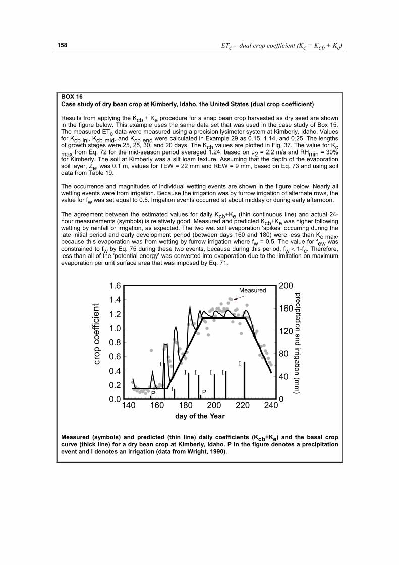
ETc -–dual crop coefficient (Kc = Kcb + Ke)
158
BOX 16 Case study of dry bean crop at Kimberly, Idaho, the United States (dual crop coefficient) Results from applying the Kcb + Ke procedure for a snap bean crop harvested as dry seed are shown in the figure below. This example uses the same data set that was used in the case study of Box 15. The measured ETc data were measured using a precision lysimeter system at Kimberly, Idaho. Values for Kcb ini, Kcb mid, and Kcb end were calculated in Example 29 as 0.15, 1.14, and 0.25. The lengths of growth stages were 25, 25, 30, and 20 days. The Kcb values are plotted in Fig. 37. The value for Kc max from Eq. 72 for the mid-season period averaged 1.24, based on u2 = 2.2 m/s and RHmin = 30% for Kimberly. The soil at Kimberly was a silt loam texture. Assuming that the depth of the evaporation soil layer, Ze, was 0.1 m, values for TEW = 22 mm and REW = 9 mm, based on Eq. 73 and using soil data from Table 19. The occurrence and magnitudes of individual wetting events are shown in the figure below. Nearly all wetting events were from irrigation. Because the irrigation was by furrow irrigation of alternate rows, the value for fw was set equal to 0.5. Irrigation events occurred at about midday or during early afternoon. The agreement between the estimated values for daily Kcb+Ke (thin continuous line) and actual 24-hour measurements (symbols) is relatively good. Measured and predicted Kcb+Ke was higher following wetting by rainfall or irrigation, as expected. The two wet soil evaporation ‘spikes’ occurring during the late initial period and early development period (between days 160 and 180) were less than Kc max, because this evaporation was from wetting by furrow irrigation where fw = 0.5. The value for few was constrained to fw by Eq. 75 during these two events, because during this period, fw < 1-fc. Therefore, less than all of the ‘potential energy’ was converted into evaporation due to the limitation on maximum evaporation per unit surface area that was imposed by Eq. 71.
140 160 180 200 220 2400.00.20.40.60.81.01.21.41.6
0
40
80
120
160
200
day of the Year
II
I
I II
I
P P
precipitation and irrigation (mm
)cr
op c
oeffi
cien
t
Measured
Measured (symbols) and predicted (thin line) daily coefficients (Kcb+Ke) and the basal crop curve (thick line) for a dry bean crop at Kimberly, Idaho. P in the figure denotes a precipitation event and I denotes an irrigation (data from Wright, 1990).
Crop evapotranspiration
159
Part C
Crop evapotranspiration under non-standard conditions
In well-managed fields, the standard conditions are generally the actual field conditions. The ETc calculated by means of the procedures described in Part B is the crop evapotranspiration under the standard field conditions.
Where the conditions encountered in the field differ from the standard conditions, a correction on ETc is required. Low soil fertility, salt toxicity, soil waterlogging, pests, diseases and the presence of hard or impenetrable soil horizons in the root zone may result in scanty plant growth and lower evapotranspiration. Soil water shortage and soil salinity may reduce soil water uptake and limit crop evapotranspiration. The evapotranspiration from small isolated stands of plants or from fields where two different crops are grown together or where mulches are used to reduce evaporation may also deviate from the crop evapotranspiration under standard conditions.
This part discusses the effect on ET of management and environmental conditions that deviate from the standard conditions. The environmental effects are described by introducing stress coefficients and by adjusting Kc to the field conditions.

160
Crop evapotranspiration
161
Chapter 8
ETc under soil water stress conditions
Forces acting on the soil water decrease its potential energy and make it less available for plant root extraction. When the soil is wet, the water has a high potential energy, is relatively free to move and is easily taken up by the plant roots. In dry soils, the water has a low potential energy and is strongly bound by capillary and absorptive forces to the soil matrix, and is less easily extracted by the crop.
When the potential energy of the soil water drops below a threshold value, the crop is said to be water stressed. The effects of soil water stress are described by multiplying the basal crop coefficient by the water stress coefficient, Ks:
oecbsdjac ET)KK(KET += (80)
For soil water limiting conditions, Ks < 1. Where there is no soil water stress, Ks = 1.
Ks describes the effect of water stress on crop transpiration. Where the single crop coefficient is used, the effect of water stress is incorporated into Kc as:
ocsdjac ETKKET = (81)
Because the water stress coefficient impacts only crop transpiration, rather than evaporation from soil, the application of Ks using Equation 80 is generally more valid than is application using Equation 81. However, in situations where evaporation from soil is not a large component of ETc, use of Equation 81 will provide reasonable results. SOIL WATER AVAILABILITY
Total available water (TAW)
Soil water availability refers to the capacity of a soil to retain water available to plants. After heavy rainfall or irrigation, the soil will drain until field capacity is reached. Field capacity is the amount of water that a well-drained soil should hold against gravitational forces, or the amount of water remaining when downward drainage has markedly decreased. In the absence of water supply, the water content in the root zone decreases as a result of water uptake by the crop. As water uptake progresses, the remaining water is held to the soil particles with greater force, lowering its potential energy and making it more difficult for the plant to extract it. Eventually, a point is reached where the crop can no longer extract the remaining water. The water uptake becomes zero when wilting point is reached. Wilting point is the water content at which plants will permanently wilt.
ETc under soil water stress conditions
162
As the water content above field capacity cannot be held against the forces of gravity and will drain and as the water content below wilting point cannot be extracted by plant roots, the total available water in the root zone is the difference between the water content at field capacity and wilting point: rWPFC Z)(1000TAW θ−θ= (82)
where TAW the total available soil water in the root zone [mm], θFC the water content at field capacity [m3 m-3], θWP the water content at wilting point [m3 m-3], Zr the rooting depth [m].
TAW is the amount of water that a crop can extract from its root zone, and its magnitude depends on the type of soil and the rooting depth. Typical ranges for field capacity and wilting point are listed in Table 19 for various soil texture classes. Ranges of the maximum effective rooting depth for various crops are given in Table 22. Readily available water (RAW)
Although water is theoretically available until wilting point, crop water uptake is reduced well before wilting point is reached. Where the soil is sufficiently wet, the soil supplies water fast enough to meet the atmospheric demand of the crop, and water uptake equals ETc. As the soil water content decreases, water becomes more strongly bound to the soil matrix and is more difficult to extract. When the soil water content drops below a threshold value, soil water can no longer be transported quickly enough towards the roots to respond to the transpiration demand and the crop begins to experience stress. The fraction of TAW that a crop can extract from the root zone without suffering water stress is the readily available soil water:
TAWpRAW = (83)
where RAW the readily available soil water in the root zone [mm], p average fraction of Total Available Soil Water (TAW) that can be
depleted from the root zone before moisture stress (reduction in ET) occurs [0 - 1].
Values for p are listed in Table 22. The factor p differs from one crop to another. The
factor p normally varies from 0.30 for shallow rooted plants at high rates of ETc (> 8 mm d-1) to 0.70 for deep rooted plants at low rates of ETc (< 3 mm d-1). A value of 0.50 for p is commonly used for many crops.
The fraction p is a function of the evaporation power of the atmosphere. At low rates of
ETc, the p values listed in Table 22 are higher than at high rates of ETc. For hot dry weather conditions, where ETc is high, p is 10-25% less than the values presented in Table 22, and the soil is still relatively wet when the stress starts to occur. When the crop evapotranspiration is low, p will be up to 20% more than the listed values. Often, a constant value is used for p for a specific growing period, rather than varying the value each day. A numerical approximation for adjusting p for ETc rate is p = pTable 22 + 0.04 (5 - ETc) where the adjusted p is limited to 0.1 ≤ p ≤ 0.8 and ETc is in mm/day. The influence of the numerical adjustment is shown in Figure 41.
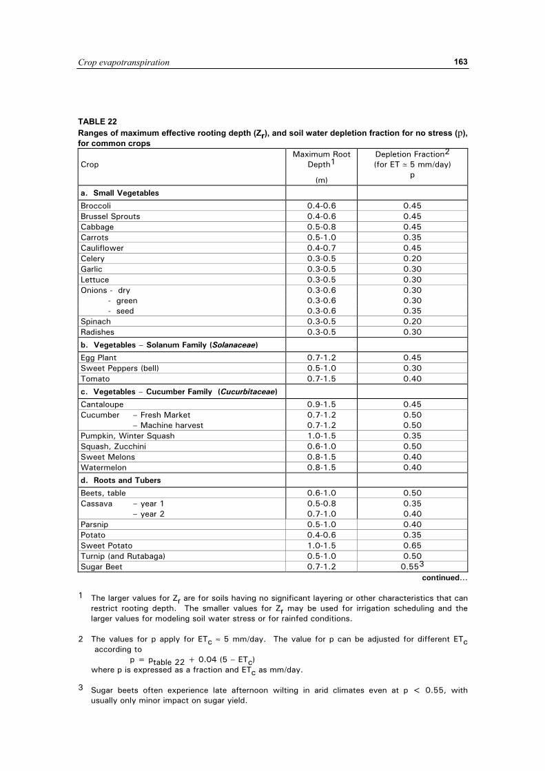
Crop evapotranspiration
163
TABLE 22 Ranges of maximum effective rooting depth (Zr), and soil water depletion fraction for no stress (p), for common crops Crop
Maximum Root Depth1
(m)
Depletion Fraction2 (for ET � 5 mm/day)
p
a. Small Vegetables
Broccoli 0.4-0.6 0.45 Brussel Sprouts 0.4-0.6 0.45 Cabbage 0.5-0.8 0.45 Carrots 0.5-1.0 0.35 Cauliflower 0.4-0.7 0.45 Celery 0.3-0.5 0.20 Garlic 0.3-0.5 0.30 Lettuce 0.3-0.5 0.30 Onions - dry 0.3-0.6 0.30 - green 0.3-0.6 0.30 - seed 0.3-0.6 0.35 Spinach 0.3-0.5 0.20 Radishes 0.3-0.5 0.30
b. Vegetables – Solanum Family (Solanaceae)
Egg Plant 0.7-1.2 0.45 Sweet Peppers (bell) 0.5-1.0 0.30 Tomato 0.7-1.5 0.40
c. Vegetables – Cucumber Family (Cucurbitaceae)
Cantaloupe 0.9-1.5 0.45 Cucumber – Fresh Market 0.7-1.2 0.50 – Machine harvest 0.7-1.2 0.50 Pumpkin, Winter Squash 1.0-1.5 0.35 Squash, Zucchini 0.6-1.0 0.50 Sweet Melons 0.8-1.5 0.40 Watermelon 0.8-1.5 0.40
d. Roots and Tubers
Beets, table 0.6-1.0 0.50 Cassava – year 1 0.5-0.8 0.35 – year 2 0.7-1.0 0.40 Parsnip 0.5-1.0 0.40 Potato 0.4-0.6 0.35 Sweet Potato 1.0-1.5 0.65 Turnip (and Rutabaga) 0.5-1.0 0.50 Sugar Beet 0.7-1.2 0.553
continued…
1 The larger values for Zr are for soils having no significant layering or other characteristics that can restrict rooting depth. The smaller values for Zr may be used for irrigation scheduling and the larger values for modeling soil water stress or for rainfed conditions.
2 The values for p apply for ETc ≈ 5 mm/day. The value for p can be adjusted for different ETc
according to p = ptable 22 + 0.04 (5 – ETc) where p is expressed as a fraction and ETc as mm/day. 3 Sugar beets often experience late afternoon wilting in arid climates even at p < 0.55, with
usually only minor impact on sugar yield.
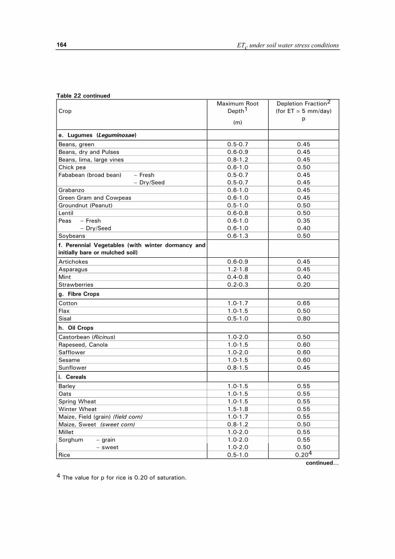
ETc under soil water stress conditions
164
Table 22 continued Crop
Maximum Root Depth1
(m)
Depletion Fraction2 (for ET � 5 mm/day)
p
e. Lugumes (Leguminosae)
Beans, green 0.5-0.7 0.45 Beans, dry and Pulses 0.6-0.9 0.45 Beans, lima, large vines 0.8-1.2 0.45 Chick pea 0.6-1.0 0.50 Fababean (broad bean) – Fresh 0.5-0.7 0.45 – Dry/Seed 0.5-0.7 0.45 Grabanzo 0.6-1.0 0.45 Green Gram and Cowpeas 0.6-1.0 0.45 Groundnut (Peanut) 0.5-1.0 0.50 Lentil 0.6-0.8 0.50 Peas – Fresh 0.6-1.0 0.35 – Dry/Seed 0.6-1.0 0.40 Soybeans 0.6-1.3 0.50
f. Perennial Vegetables (with winter dormancy and initially bare or mulched soil)
Artichokes 0.6-0.9 0.45 Asparagus 1.2-1.8 0.45 Mint 0.4-0.8 0.40 Strawberries 0.2-0.3 0.20
g. Fibre Crops
Cotton 1.0-1.7 0.65 Flax 1.0-1.5 0.50 Sisal 0.5-1.0 0.80
h. Oil Crops
Castorbean (Ricinus) 1.0-2.0 0.50 Rapeseed, Canola 1.0-1.5 0.60 Safflower 1.0-2.0 0.60 Sesame 1.0-1.5 0.60 Sunflower 0.8-1.5 0.45
i. Cereals
Barley 1.0-1.5 0.55 Oats 1.0-1.5 0.55 Spring Wheat 1.0-1.5 0.55
Winter Wheat 1.5-1.8 0.55
Maize, Field (grain) (field corn) 1.0-1.7 0.55 Maize, Sweet (sweet corn) 0.8-1.2 0.50 Millet 1.0-2.0 0.55 Sorghum – grain 1.0-2.0 0.55 – sweet 1.0-2.0 0.50 Rice 0.5-1.0 0.204
continued… 4 The value for p for rice is 0.20 of saturation.
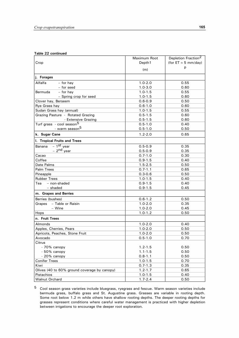
Crop evapotranspiration
165
Table 22 continued Crop
Maximum Root Depth1
(m)
Depletion Fraction2 (for ET � 5 mm/day)
p
j. Forages
Alfalfa – for hay 1.0-2.0 0.55 – for seed 1.0-3.0 0.60 Bermuda – for hay 1.0-1.5 0.55 – Spring crop for seed 1.0-1.5 0.60 Clover hay, Berseem 0.6-0.9 0.50 Rye Grass hay 0.6-1.0 0.60 Sudan Grass hay (annual) 1.0-1.5 0.55 Grazing Pasture - Rotated Grazing 0.5-1.5 0.60 - Extensive Grazing 0.5-1.5 0.60 Turf grass - cool season5 0.5-1.0 0.40 - warm season5 0.5-1.0 0.50
k. Sugar Cane 1.2-2.0 0.65
l. Tropical Fruits and Trees
Banana – 1st year 0.5-0.9 0.35 – 2nd year 0.5-0.9 0.35 Cacao 0.7-1.0 0.30 Coffee 0.9-1.5 0.40 Date Palms 1.5-2.5 0.50 Palm Trees 0.7-1.1 0.65 Pineapple 0.3-0.6 0.50 Rubber Trees 1.0-1.5 0.40 Tea – non-shaded 0.9-1.5 0.40 – shaded 0.9-1.5 0.45
m. Grapes and Berries
Berries (bushes) 0.6-1.2 0.50 Grapes – Table or Raisin 1.0-2.0 0.35 – Wine 1.0-2.0 0.45 Hops 1.0-1.2 0.50
n. Fruit Trees
Almonds 1.0-2.0 0.40 Apples, Cherries, Pears 1.0-2.0 0.50 Apricots, Peaches, Stone Fruit 1.0-2.0 0.50 Avocado 0.5-1.0 0.70 Citrus - 70% canopy 1.2-1.5 0.50 - 50% canopy 1.1-1.5 0.50 - 20% canopy 0.8-1.1 0.50 Conifer Trees 1.0-1.5 0.70 Kiwi 0.7-1.3 0.35 Olives (40 to 60% ground coverage by canopy) 1.2-1.7 0.65 Pistachios 1.0-1.5 0.40 Walnut Orchard 1.7-2.4 0.50
5 Cool season grass varieties include bluegrass, ryegrass and fescue. Warm season varieties include
bermuda grass, buffalo grass and St. Augustine grass. Grasses are variable in rooting depth. Some root below 1.2 m while others have shallow rooting depths. The deeper rooting depths for grasses represent conditions where careful water management is practiced with higher depletion between irrigations to encourage the deeper root exploration.
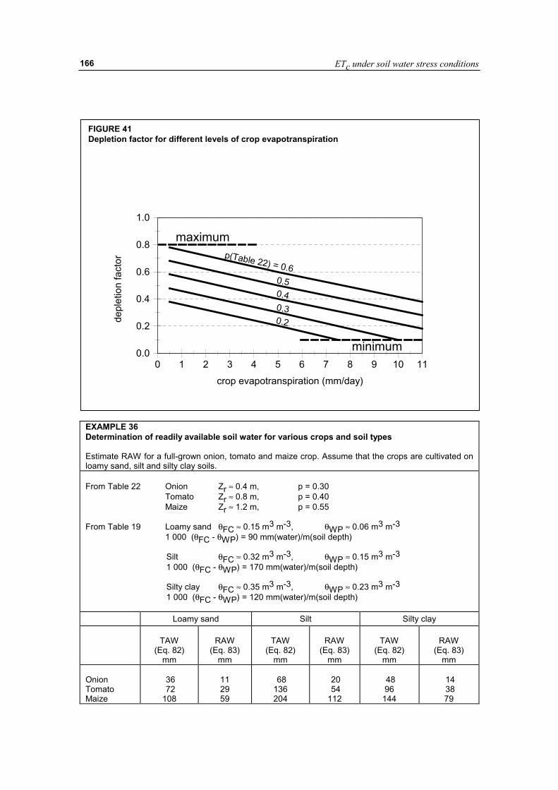
ETc under soil water stress conditions
166
EXAMPLE 36 Determination of readily available soil water for various crops and soil types Estimate RAW for a full-grown onion, tomato and maize crop. Assume that the crops are cultivated on loamy sand, silt and silty clay soils. From Table 22 Onion Zr ≈ 0.4 m, p = 0.30 Tomato Zr ≈ 0.8 m, p = 0.40 Maize Zr ≈ 1.2 m, p = 0.55 From Table 19 Loamy sand θFC ≈ 0.15 m3 m-3, θWP ≈ 0.06 m3 m-3 1 000 (θFC - θWP) = 90 mm(water)/m(soil depth)
Silt θFC ≈ 0.32 m3 m-3, θWP ≈ 0.15 m3 m-3 1 000 (θFC - θWP) = 170 mm(water)/m(soil depth) Silty clay θFC ≈ 0.35 m3 m-3, θWP ≈ 0.23 m3 m-3 1 000 (θFC - θWP) = 120 mm(water)/m(soil depth)
Loamy sand Silt Silty clay
TAW (Eq. 82)
mm
RAW
(Eq. 83) mm
TAW
(Eq. 82) mm
RAW
(Eq. 83) mm
TAW
(Eq. 82) mm
RAW
(Eq. 83) mm
Onion Tomato Maize
36 72 108
11 29 59
68 136 204
20 54 112
48 96
144
14 38 79
FIGURE 41 Depletion factor for different levels of crop evapotranspiration
0 1 2 3 4 5 6 7 8 9 10 11crop evapotranspiration (mm/day)
0.0
0.2
0.4
0.6
0.8
1.0
depl
etio
n fa
ctor
maximum
minimum
0.50.40.30.2
p(Table 22) = 0.6
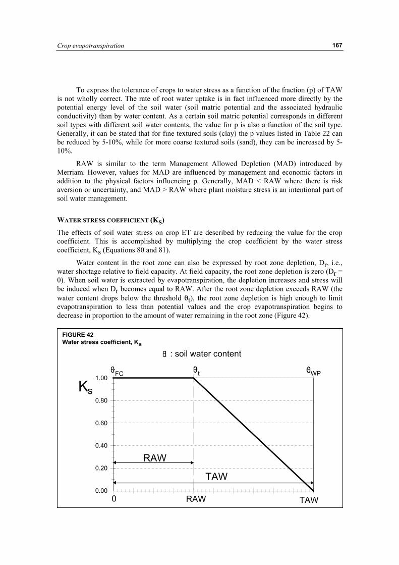
Crop evapotranspiration
167
To express the tolerance of crops to water stress as a function of the fraction (p) of TAW is not wholly correct. The rate of root water uptake is in fact influenced more directly by the potential energy level of the soil water (soil matric potential and the associated hydraulic conductivity) than by water content. As a certain soil matric potential corresponds in different soil types with different soil water contents, the value for p is also a function of the soil type. Generally, it can be stated that for fine textured soils (clay) the p values listed in Table 22 can be reduced by 5-10%, while for more coarse textured soils (sand), they can be increased by 5-10%.
RAW is similar to the term Management Allowed Depletion (MAD) introduced by Merriam. However, values for MAD are influenced by management and economic factors in addition to the physical factors influencing p. Generally, MAD < RAW where there is risk aversion or uncertainty, and MAD > RAW where plant moisture stress is an intentional part of soil water management. WATER STRESS COEFFICIENT (KS)
The effects of soil water stress on crop ET are described by reducing the value for the crop coefficient. This is accomplished by multiplying the crop coefficient by the water stress coefficient, Ks (Equations 80 and 81).
Water content in the root zone can also be expressed by root zone depletion, Dr, i.e., water shortage relative to field capacity. At field capacity, the root zone depletion is zero (Dr = 0). When soil water is extracted by evapotranspiration, the depletion increases and stress will be induced when Dr becomes equal to RAW. After the root zone depletion exceeds RAW (the water content drops below the threshold θt), the root zone depletion is high enough to limit evapotranspiration to less than potential values and the crop evapotranspiration begins to decrease in proportion to the amount of water remaining in the root zone (Figure 42).
FIGURE 42 Water stress coefficient, Ks
0.00
0.20
0.40
0.60
0.80
1.00
: soil water content
FC t WP
Ks
0 RAW TAW
RAW
TAW
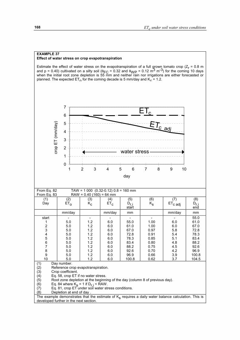
ETc under soil water stress conditions
168
EXAMPLE 37 Effect of water stress on crop evapotranspiration Estimate the effect of water stress on the evapotranspiration of a full grown tomato crop (Zr = 0.8 m and p = 0.40) cultivated on a silty soil (θFC = 0.32 and θWP = 0.12 m3 m-3) for the coming 10 days when the initial root zone depletion is 55 mm and neither rain nor irrigations are either forecasted or planned. The expected ETo for the coming decade is 5 mm/day and Kc = 1.2.
1 2 3 4 5 6 7 8 9 10day
0
1
2
3
4
5
6
7
crop
ET
(mm
/day
)
ETc
ETc adj
water stress
From Eq. 82 TAW = 1 000 (0.32-0.12) 0.8 = 160 mm From Eq. 83 RAW = 0.40 (160) = 64 mm
(1) Day
(2) ETo
(3) Kc
(4) ETc
(5) Dr,i start
(6) Ks
(7) ETc adj
(8) Dr,i end
mm/day mm/day mm mm/day mm start
1 2 3 4 5 6 7 8 9 10
- 5.0 5.0 5.0 5.0 5.0 5.0 5.0 5.0 5.0 5.0
- 1.2 1.2 1.2 1.2 1.2 1.2 1.2 1.2 1.2 1.2
- 6.0 6.0 6.0 6.0 6.0 6.0 6.0 6.0 6.0 6.0
- 55.0 61.0 67.0 72.8 78.3 83.4 88.2 92.6 96.9
100.8
- 1.00 1.00 0.97 0.91 0.85 0.80 0.75 0.70 0.66 0.62
- 6.0 6.0 5.8 5.4 5.1 4.8 4.5 4.2 3.9 3.7
55.0 61.0 67.0 72.8 78.3 83.4 88.2 92.6 96.9
100.8 104.5
(1) Day number. (2) Reference crop evapotranspiration. (3) Crop coefficient. (4) Eq. 58, crop ET if no water stress. (5) Root zone depletion at the beginning of the day (column 8 of previous day). (6) Eq. 84 where Ks = 1 if Dr,i < RAW. (7) Eq. 81, crop ET under soil water stress conditions. (8) Depletion at end of day . The example demonstrates that the estimate of Ks requires a daily water balance calculation. This is developed further in the next section.
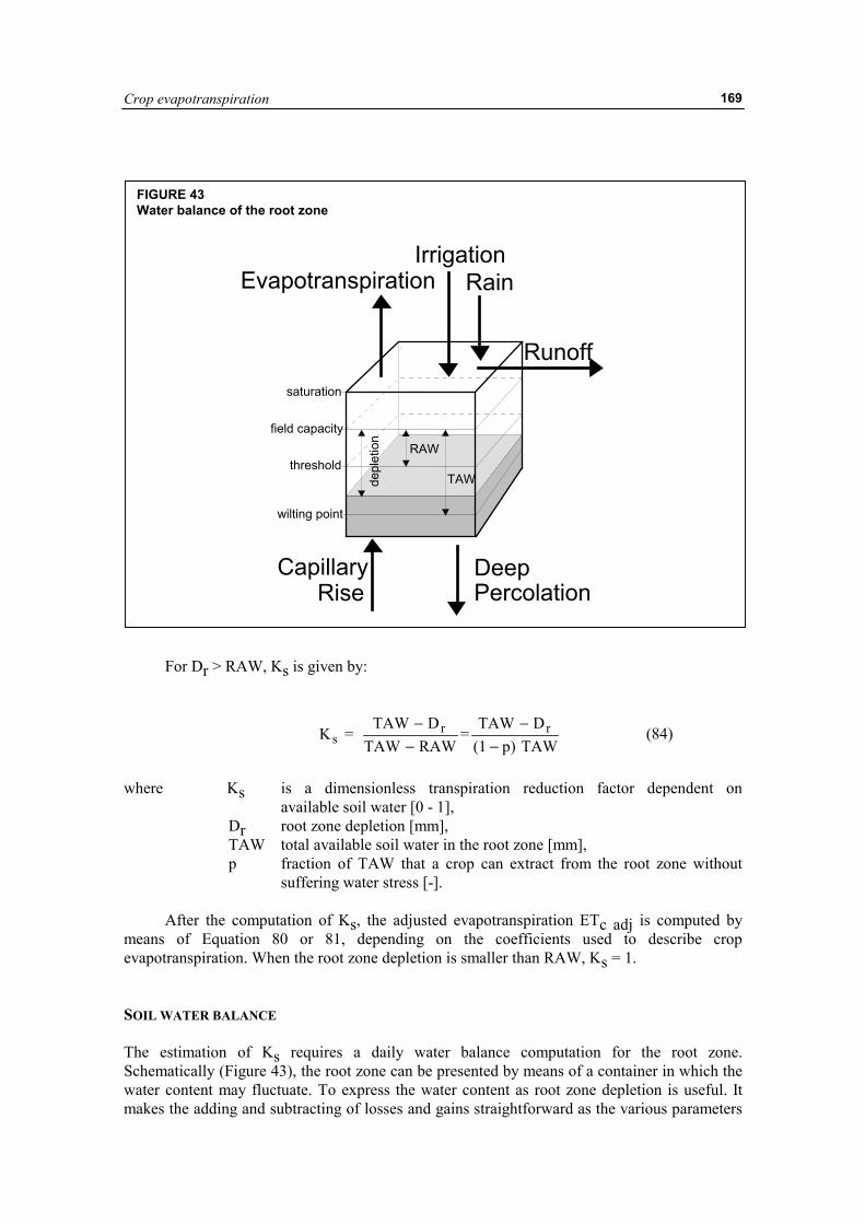
Crop evapotranspiration
169
For Dr > RAW, Ks is given by:
TAW)p(1
DTAW=
RAWTAWDTAW
=K rrs −
−−
− (84)
where Ks is a dimensionless transpiration reduction factor dependent on
available soil water [0 - 1], Dr root zone depletion [mm], TAW total available soil water in the root zone [mm], p fraction of TAW that a crop can extract from the root zone without
suffering water stress [-].
After the computation of Ks, the adjusted evapotranspiration ETc adj is computed by means of Equation 80 or 81, depending on the coefficients used to describe crop evapotranspiration. When the root zone depletion is smaller than RAW, Ks = 1. SOIL WATER BALANCE The estimation of Ks requires a daily water balance computation for the root zone. Schematically (Figure 43), the root zone can be presented by means of a container in which the water content may fluctuate. To express the water content as root zone depletion is useful. It makes the adding and subtracting of losses and gains straightforward as the various parameters
FIGURE 43 Water balance of the root zone
depl
etio
n
RAW
TAW
saturation
field capacity
threshold
wilting point
EvapotranspirationIrrigation
Rain
Runoff
Capillary DeepPercolationRise
ETc under soil water stress conditions
170
of the soil water budget are usually expressed in terms of water depth. Rainfall, irrigation and capillary rise of groundwater towards the root zone add water to the root zone and decrease the root zone depletion. Soil evaporation, crop transpiration and percolation losses remove water from the root zone and increase the depletion. The daily water balance, expressed in terms of depletion at the end of the day is:
ii,ciii1-i,ri,r DP+ETCRIRO)(PDD +−−−−= (85) where Dr,i root zone depletion at the end of day i [mm],
Dr,i-1 water content in the root zone at the end of the previous day, i-1 [mm], Pi precipitation on day i [mm], ROi runoff from the soil surface on day i [mm], Ii net irrigation depth on day i that infiltrates the soil [mm], CRi capillary rise from the groundwater table on day i [mm], ETc,i crop evapotranspiration on day i [mm], DPi water loss out of the root zone by deep percolation on day i [mm].
Limits on Dr, i In Figure 43 it is assumed that water can be stored in the root zone until field capacity is reached. Although following heavy rain or irrigation the water content might temporally exceed field capacity, the total amount of water above field capacity is assumed to be lost the same day by deep percolation, following any ET for that day. By assuming that the root zone is at field capacity following heavy rain or irrigation, the minimum value for the depletion Dr,i is zero. As a result of percolation and evapotranspiration, the water content in the root zone will gradually decrease and the root zone depletion will increase. In the absence of any wetting event, the water content will steadily reach its minimum value θWP. At that moment no water is left for evapotranspiration in the root zone, Ks becomes zero, and the root zone depletion has reached its maximum value TAW. The limits imposed on Dr,i are consequently:
TAWD0 i,r ≤≤ (86) Initial depletion To initiate the water balance for the root zone, the initial depletion Dr,i-1 should be estimated. The initial depletion can be derived from measured soil water content by:
r1-iFC1-i,r Z)(1000D θ−θ= (87) where θi-1 is the average soil water content for the effective root zone. Following heavy rain or irrigation, the user can assume that the root zone is near field capacity, i.e., Dr,i-1 ≈ 0. Precipitation (P), runoff (RO) and irrigation (I) Pi is equivalent to daily precipitation. Daily precipitation in amounts less than about 0.2 ETo is normally entirely evaporated and can usually be ignored in the water balance calculations especially when the single crop coefficient approach is being used. Ii is equivalent to the mean
Crop evapotranspiration
171
infiltrated irrigation depth expressed for the entire field surface. Runoff from the surface during precipitation can be predicted using standard procedures from hydrological texts. Capillary rise (CR)
The amount of water transported upwards by capillary rise from the water table to the root zone depends on the soil type, the depth of the water table and the wetness of the root zone. CR can normally be assumed to be zero when the water table is more than about 1 m below the bottom of the root zone. Some information on CR was presented in FAO Irrigation and Drainage Paper No. 24. CR will be a topic in a future FAO publication. Evapotranspiration (ETc)
Where the soil water depletion is smaller than RAW, the crop evapotranspiration equals ETc = Kc ETo. As soon as Dr,i exceeds RAW, the crop evapotranspiration is reduced and ETc can be computed from Equation 80 or 81. Deep percolation (DP)
Following heavy rain or irrigation, the soil water content in the root zone might exceed field capacity. In this simple procedure it is assumed that the soil water content is at θFC within the same day of the wetting event, so that the depletion Dr, i in Equation 85 becomes zero. Therefore, following heavy rain or irrigation 0DETI)RO(PPD 1-i,ri,ciiii ≥−−+−= (88)
As long as the soil water content in the root zone is below field capacity (i.e., Dr, i > 0),
the soil will not drain and DPi = 0.
The DPi term in Equations 85 and 88 is not to be confused with the DPe,i term used in Equations 77 and 79 for the evaporation layer. Both terms can be calculated at the same time, but are independent of one another. FORECASTING OR ALLOCATING IRRIGATIONS
Irrigation is required when rainfall is insufficient to compensate for the water lost by evapotranspiration. The primary objective of irrigation is to apply water at the right period and in the right amount. By calculating the soil water balance of the root zone on a daily basis (Equation 85), the timing and the depth of future irrigations can be planned. To avoid crop water stress, irrigations should be applied before or at the moment when the readily available soil water is depleted (Dr,i ≤ RAW). To avoid deep percolation losses that may leach relevant nutrients out of the root zone, the net irrigation depth should be smaller than or equal to the root zone depletion (Ii ≤ Dr,i).
Example 38 illustrates the application of a water balance of the root zone to predict irrigation dates to avoid water stress. The example utilizes various calculations for Ke from Example 35. A complete “spreadsheet” that includes all necessary calculations for predicting both irrigation schedules and to predict Kc = Kcb + Ke for daily timesteps is presented in Annex 8.
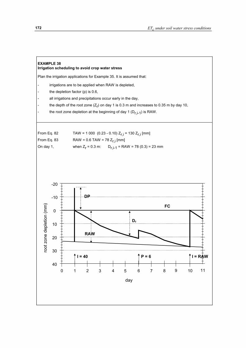
ETc under soil water stress conditions
172
EXAMPLE 38 Irrigation scheduling to avoid crop water stress Plan the irrigation applications for Example 35. It is assumed that: - irrigations are to be applied when RAW is depleted,
- the depletion factor (p) is 0.6,
- all irrigations and precipitations occur early in the day,
- the depth of the root zone (Zr) on day 1 is 0.3 m and increases to 0.35 m by day 10,
- the root zone depletion at the beginning of day 1 (Dr,i-1) is RAW. From Eq. 82 TAW = 1 000 (0.23 - 0.10) Zr,i = 130 Zr,i [mm]
From Eq. 83 RAW = 0.6 TAW = 78 Zr,i [mm]
On day 1, when Zr = 0.3 m: Dr,i-1 = RAW = 78 (0.3) = 23 mm
0 2 4 6 8 10
day
111 3 5 7 940
30
20
10
0
-10
-20
root
zon
e de
plet
ion
(mm
)
I = 40 I = RAWP = 6
RAW
DP
FC
Dr
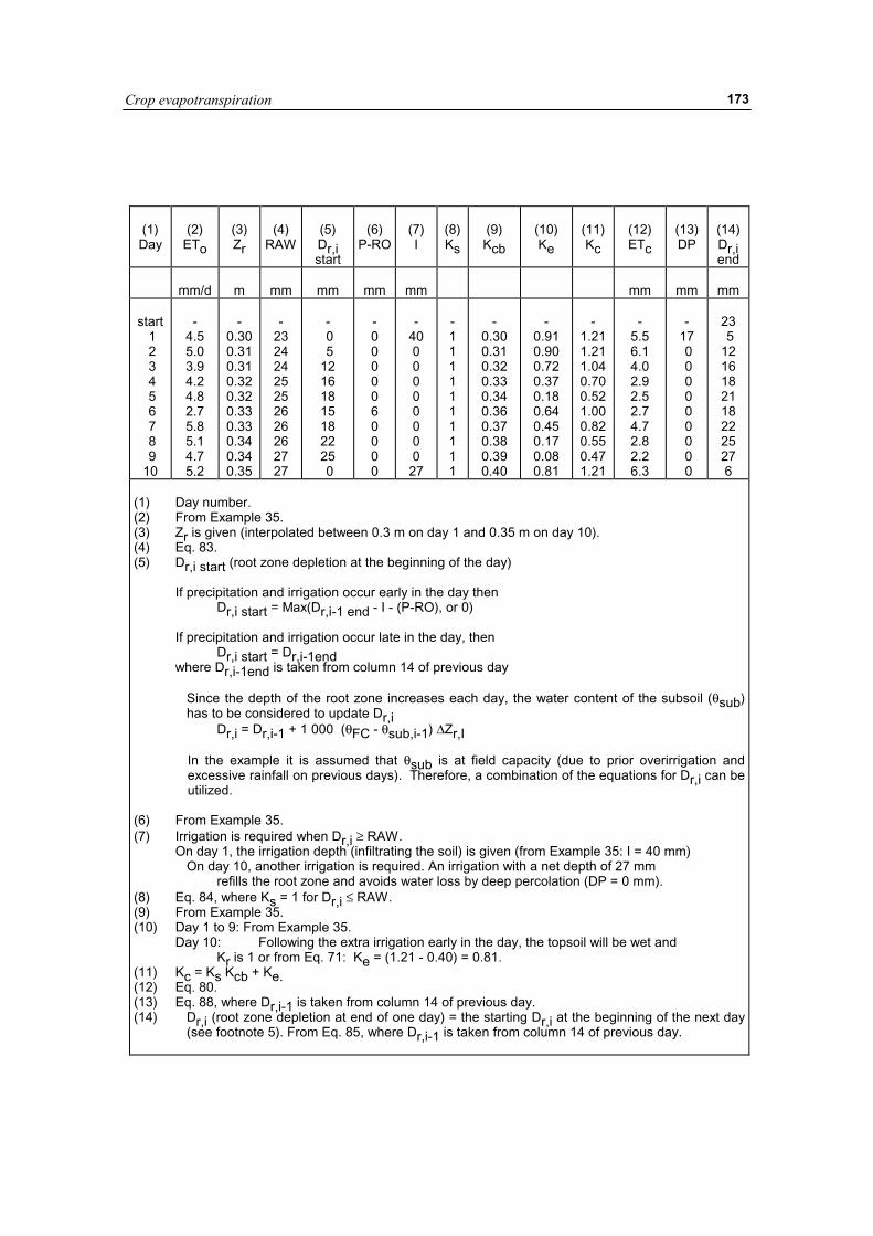
Crop evapotranspiration
173
(1) Day
(2)
ETo
(3) Zr
(4)
RAW
(5) Dr,i start
(6)
P-RO
(7) I
(8) Ks
(9) Kcb
(10) Ke
(11) Kc
(12) ETc
(13) DP
(14) Dr,i end
mm/d
m
mm
mm
mm
mm
mm
mm
mm
start
1 2 3 4 5 6 7 8 9 10
-
4.5 5.0 3.9 4.2 4.8 2.7 5.8 5.1 4.7 5.2
-
0.30 0.31 0.31 0.32 0.32 0.33 0.33 0.34 0.34 0.35
-
23 24 24 25 25 26 26 26 27 27
- 0 5 12 16 18 15 18 22 25 0
- 0 0 0 0 0 6 0 0 0 0
-
40 0 0 0 0 0 0 0 0
27
- 1 1 1 1 1 1 1 1 1 1
-
0.30 0.31 0.32 0.33 0.34 0.36 0.37 0.38 0.39 0.40
-
0.91 0.90 0.72 0.37 0.18 0.64 0.45 0.17 0.08 0.81
-
1.21 1.21 1.04 0.70 0.52 1.00 0.82 0.55 0.47 1.21
-
5.5 6.1 4.0 2.9 2.5 2.7 4.7 2.8 2.2 6.3
-
17 0 0 0 0 0 0 0 0 0
23 5 12 16 18 21 18 22 25 27 6
(1) Day number. (2) From Example 35. (3) Zr is given (interpolated between 0.3 m on day 1 and 0.35 m on day 10). (4) Eq. 83. (5) Dr,i start (root zone depletion at the beginning of the day) If precipitation and irrigation occur early in the day then Dr,i start = Max(Dr,i-1 end - I - (P-RO), or 0) If precipitation and irrigation occur late in the day, then Dr,i start = Dr,i-1end where Dr,i-1end is taken from column 14 of previous day Since the depth of the root zone increases each day, the water content of the subsoil (θsub)
has to be considered to update Dr,i Dr,i = Dr,i-1 + 1 000 (θFC - θsub,i-1) ∆Zr,I
In the example it is assumed that θsub is at field capacity (due to prior overirrigation and excessive rainfall on previous days). Therefore, a combination of the equations for Dr,i can be utilized.
(6) From Example 35. (7) Irrigation is required when Dr,i ≥ RAW. On day 1, the irrigation depth (infiltrating the soil) is given (from Example 35: I = 40 mm) On day 10, another irrigation is required. An irrigation with a net depth of 27 mm
refills the root zone and avoids water loss by deep percolation (DP = 0 mm). (8) Eq. 84, where Ks = 1 for Dr,i ≤ RAW. (9) From Example 35. (10) Day 1 to 9: From Example 35. Day 10: Following the extra irrigation early in the day, the topsoil will be wet and Kr is 1 or from Eq. 71: Ke = (1.21 - 0.40) = 0.81. (11) Kc = Ks Kcb + Ke. (12) Eq. 80. (13) Eq. 88, where Dr,i-1 is taken from column 14 of previous day. (14) Dr,i (root zone depletion at end of one day) = the starting Dr,i at the beginning of the next day
(see footnote 5). From Eq. 85, where Dr,i-1 is taken from column 14 of previous day.
ETc under soil water stress conditions
174
EFFECTS OF SOIL SALINITY Salts in the soil water solution can reduce evapotranspiration by making soil water less "available" for plant root extraction. Salts have an affinity for water and hence additional force is required for the crop to extract water from a saline soil. The presence of salts in the soil water solution reduces the total potential energy of the soil water solution. In addition, some salts cause toxic effects in plants and can reduce plant metabolism and growth. A function is presented here that predicts the reduction in evapotranspiration caused by salinity of soil water. The function is derived by combining yield-salinity equations from the FAO Irrigation and Drainage Paper No29 with yield-ET equations from FAO Irrigation and Drainage Paper No33. The resulting equation provides a first approximation of the reduction in evapotranspiration expected under various salinity conditions.
There is evidence that crop yield and transpiration are not as sensitive to low osmotic potential as they are to low matric potential. Under saline conditions, many plants are able to partially compensate for low osmotic potential of the soil water by building up higher internal solute contents. This is done by absorbing ions from the soil solution and by synthesizing organic osmolytes. Both of these reactions reduce the impact of osmotic potential on water availability. However, synthesis of organic osmolytes does require expenditure of metabolic energy. Therefore plant growth is often reduced under saline conditions. The reduced plant growth impacts transpiration by reducing ground cover and is sometimes additionally due to partial stomatal closure.
Other impacts of salts in the soil include direct sodium and chloride toxicities and induced nutrient deficiencies. These deficiencies reduce plant growth by reducing the rate of leaf elongation, the enlargement, and the division of cells in leaves. The modality depends on the method of irrigation. With sprinkler irrigation, adsorption of sodium and chloride through the leaf can result in toxic conditions for all crop species. With surface or trickle irrigaiton, direct toxic conditions generally occur only in vine and tree crops; however, high levels of sodium can induce calcium deficieincies for all crop species.
Since salt concentration changes as the soil water content changes, soil salinity is normally measured and expressed on the basis of the electrical conductivity of the saturation extract of the soil (ECe). The ECe is defined as the electrical conductivity of the soil water solution after the addition of a sufficient quantity of distilled water to bring the soil water content to saturation. ECe is typically expressed in deciSiemens per meter (dS m-1). Under optimum management conditions, crop yields remain at potential levels until a specific, threshold electrical conductivity of the saturation soil water extract (ECe threshold) is reached. If the average ECe of the root zone increases above this critical threshold value, the yield is presumed to begin to decrease linearly in proportion to the increase in salinity. The rate of decrease in yield with increase in salinity is usually expressed as a slope, b, having units of % reduction in yield per dS/m increase in ECe.
All plants do not respond to salinity in a similar manner; some crops can produce acceptable yields at much higher soil salinity levels than others. This is because some crops are better able to make the needed osmotic adjustments that enable them to extract more water from a saline soil, or they may be more tolerant of some of the toxic effects of salinity. Salt tolerance for many agricultural crops are provided in the FAO Irrigation and Drainage Papers No. 33 and 48. The ECe,threshold and slope b from these sources are listed in Table 23.
Crop evapotranspiration
175
As can be observed from the data in Table 23, there is an 8 to 10-fold range in salt tolerance of agricultural crops. The effect of soil salinity on yield and crop evapotranspiration is hence crop specific.
The ECe, threshold and b parameters in Table 23 were determined primarily in research
experiments using nearly steady-state irrigation where soil water contents were maintained at levels close to field capacity. However, under most types of irrigation scheduling for sprinkler and surface irrigation, the soil water content is typically depleted to well below field capacity, so that the EC of the soil water solution, ECsw, increases prior to irrigation, even though the EC of the saturation extract does not change. The increased salt concentration in the soil water solution reduces the osmotic potential of the soil water solution (it becomes more negative), so that the plant must expend more metabolic energy and may exert more mechanical force to absorb water. In addition, metabolic and toxic effects of salts on plants may become more pronounced as the soil dries and concentrations increase. However, the variation in soil water content during an irrigation interval has not been found to strongly influence crop evapotranspiration. This is because of the rise of soil water content to levels that are above that experienced under steady state irrigation early in a long irrigation interval. There is a similar, counteractive decrease in soil water content later in a long irrigation interval. In addition, the distribution of salts in the root zone under low frequency irrigation can reduce salinity impacts during the first portion of the irrigation interval. Also, under high frequency irrigation of the soil surface, soil evaporation losses are higher. Consequently, given the same application depth, the leaching fraction is reduced. For these reasons, the length of irrigation interval and the change in EC of soil water during the interval have usually not been found to be factors in the reduction of ET, given that the same depths of water are infiltrated into the root zone over time.
In some cases, increased evaporation under high frequency irrigation of the soil surface can counteract reductions in Kc caused by high ECe of the root zone. Under these conditions, the total Kc and ETc are not very different from the non-saline, standard conditions under less frequent irrigation, even though crop yields and crop transpiration are reduced. Because of this, under saline conditions, the Ks reducing factor should only be applied with the dual Kc approach.
In review articles on impacts of salinity on crop production, Letey et al. (1985) and Shalhevet (1994) concluded that effects of soil salinity and water stress are generally additive in their impacts on crop evapotranspiration. Therefore, the same yield-ET functions may hold for both water shortage induced stress and for salinity induced stress. YIELD-SALINITY RELATIONSHIP A widely practiced approach for predicting the reduction in crop yield due to salinity has been described in the FAO Irrigation and Drainage Paper No29. The approach presumes that, under optimum management conditions, crop yields remain at potential levels until a specific, threshold electrical conductivity of the soil water solution is reached. When salinity increases beyond this threshold, crop yields are presumed to decrease linearly in proportion to the increase in salinity. The soil water salinity is expressed as the electrical conductivity of the saturation extract, ECe. In equation form, the procedure followed in FAO Irrigation and Drainage Paper No29 is:
ETc under soil water stress conditions
176
( )100
bECEC1YY
thresholdeem
a −−= (89)
for conditions where ECe > ECe threshold where:
Ya actual crop yield Ym maximum expected crop yield when ECe < ECe threshold ECe mean electrical conductivity of the saturation extract for the root zone
[dS m-1] ECe threshold electrical conductivity of the saturation extract at the threshold of ECe
when crop yield first reduces below Ym [dS m-1] b reduction in yield per increase in ECe [%/(dS m-1)] Values for ECe threshold and b have been provided in the FAO Irrigation and Drainage Paper No29 and 48 and are listed in Table 23 for many agricultural crops.
Salinity-yield data from the FAO Irrigation and Drainage papers Nos. 29 and 48 were mostly from studies where soil water content was held at about –3 m potential (-30 kPa) or higher at the 0.3 to 0.6 m depth, depending on the crop. However, these papers indicate that for most crops, the data are transferable to typical field situations where the readily available soil water (RAW) is depleted between irrigations. YIELD-MOISTURE STRESS RELATIONSHIP
A simple, linear crop-water production function was introduced in the FAO Irrigation and Drainage Paper No33 to predict the reduction in crop yield when crop stress was caused by a shortage of soil water:
���
����
�−=�
��
����
�−
c
adjcy
m ETET
1KYYa1 (90)
where: Ky a yield response factor [-] ETc adj adjusted (actual) crop evapotranspiration [mm d-1] ETc crop evapotranspiration for standard conditions (no water stress) [mm d-1] Ky is a factor that describes the reduction in relative yield according to the reduction in ETc caused by soil water shortage. In FAO No33, Ky values are crop specific and may vary over the growing season. In general, the decrease in yield due to water deficit during the vegetative and ripening period is relatively small, while during the flowering and yield formation periods it will be large. Values for Ky for individual growth periods and for the complete growing season have been included in the FAO Irrigation and Drainage Paper No33. Seasonal values for Ky are summarized in Table 24. COMBINED SALINITY-ET REDUCTION RELATIONSHIP
No water stress (Dr < RAW)
When salinity stress occurs without water stress, Equations 89 and 90 can be combined and solved for an equivalent Ks, where Ks = ETc adj/ETc:
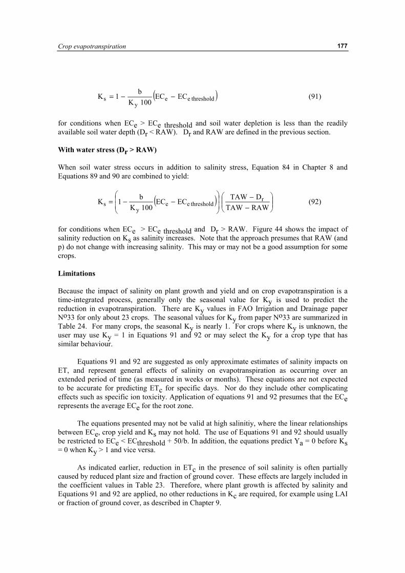
Crop evapotranspiration
177
( )thresholdeey
s ECEC100K
b1K −−= (91)
for conditions when ECe > ECe threshold and soil water depletion is less than the readily available soil water depth (Dr < RAW). Dr and RAW are defined in the previous section. With water stress (Dr > RAW) When soil water stress occurs in addition to salinity stress, Equation 84 in Chapter 8 and Equations 89 and 90 are combined to yield:
( ) ���
����
�
−−
��
�
�
��
�
�−−=
RAWTAWDTAWECEC
100Kb1K r
thresholdeey
s (92)
for conditions when ECe > ECe threshold and Dr > RAW. Figure 44 shows the impact of salinity reduction on Ks as salinity increases. Note that the approach presumes that RAW (and p) do not change with increasing salinity. This may or may not be a good assumption for some crops. Limitations Because the impact of salinity on plant growth and yield and on crop evapotranspiration is a time-integrated process, generally only the seasonal value for Ky is used to predict the reduction in evapotranspiration. There are Ky values in FAO Irrigation and Drainage paper No33 for only about 23 crops. The seasonal values for Ky from paper No33 are summarized in Table 24. For many crops, the seasonal Ky is nearly 1. For crops where Ky is unknown, the user may use Ky = 1 in Equations 91 and 92 or may select the Ky for a crop type that has similar behaviour. Equations 91 and 92 are suggested as only approximate estimates of salinity impacts on ET, and represent general effects of salinity on evapotranspiration as occurring over an extended period of time (as measured in weeks or months). These equations are not expected to be accurate for predicting ETc for specific days. Nor do they include other complicating effects such as specific ion toxicity. Application of equations 91 and 92 presumes that the ECe represents the average ECe for the root zone. The equations presented may not be valid at high salinitiy, where the linear relationships between ECe, crop yield and Ks may not hold. The use of Equations 91 and 92 should usually be restricted to ECe < ECthreshold + 50/b. In addition, the equations predict Ya = 0 before Ks = 0 when Ky > 1 and vice versa.
As indicated earlier, reduction in ETc in the presence of soil salinity is often partially caused by reduced plant size and fraction of ground cover. These effects are largely included in the coefficient values in Table 23. Therefore, where plant growth is affected by salinity and Equations 91 and 92 are applied, no other reductions in Kc are required, for example using LAI or fraction of ground cover, as described in Chapter 9.
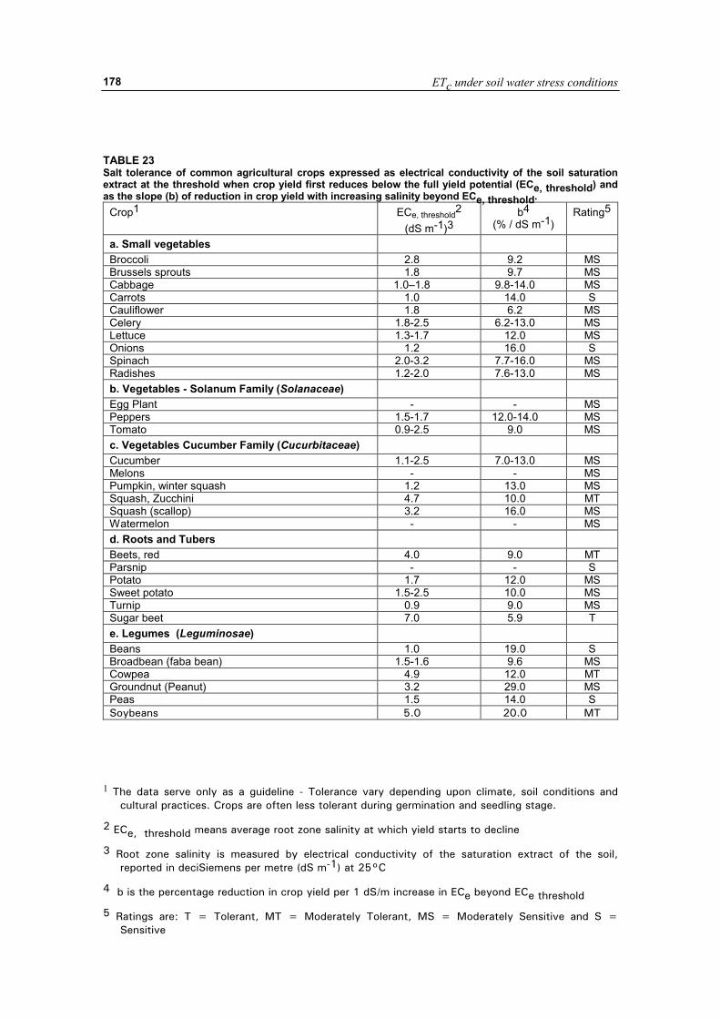
ETc under soil water stress conditions
178
TABLE 23 Salt tolerance of common agricultural crops expressed as electrical conductivity of the soil saturation extract at the threshold when crop yield first reduces below the full yield potential (ECe, threshold) and as the slope (b) of reduction in crop yield with increasing salinity beyond ECe, threshold.
Crop1 ECe, threshold2 (dS m-1)3
b4 (% / dS m-1)
Rating5
a. Small vegetables Broccoli 2.8 9.2 MS Brussels sprouts 1.8 9.7 MS Cabbage 1.0–1.8 9.8-14.0 MS Carrots 1.0 14.0 S Cauliflower 1.8 6.2 MS Celery 1.8-2.5 6.2-13.0 MS Lettuce 1.3-1.7 12.0 MS Onions 1.2 16.0 S Spinach 2.0-3.2 7.7-16.0 MS Radishes 1.2-2.0 7.6-13.0 MS b. Vegetables - Solanum Family (Solanaceae) Egg Plant - - MS Peppers 1.5-1.7 12.0-14.0 MS Tomato 0.9-2.5 9.0 MS c. Vegetables Cucumber Family (Cucurbitaceae) Cucumber 1.1-2.5 7.0-13.0 MS Melons - - MS Pumpkin, winter squash 1.2 13.0 MS Squash, Zucchini 4.7 10.0 MT Squash (scallop) 3.2 16.0 MS Watermelon - - MS d. Roots and Tubers Beets, red 4.0 9.0 MT Parsnip - - S Potato 1.7 12.0 MS Sweet potato 1.5-2.5 10.0 MS Turnip 0.9 9.0 MS Sugar beet 7.0 5.9 T e. Legumes (Leguminosae) Beans 1.0 19.0 S Broadbean (faba bean) 1.5-1.6 9.6 MS Cowpea 4.9 12.0 MT Groundnut (Peanut) 3.2 29.0 MS Peas 1.5 14.0 S Soybeans 5.0 20.0 MT
1 The data serve only as a guideline - Tolerance vary depending upon climate, soil conditions and
cultural practices. Crops are often less tolerant during germination and seedling stage.
2 ECe, threshold means average root zone salinity at which yield starts to decline
3 Root zone salinity is measured by electrical conductivity of the saturation extract of the soil,
reported in deciSiemens per metre (dS m-1) at 25°C
4 b is the percentage reduction in crop yield per 1 dS/m increase in ECe beyond ECe threshold
5 Ratings are: T = Tolerant, MT = Moderately Tolerant, MS = Moderately Sensitive and S = Sensitive
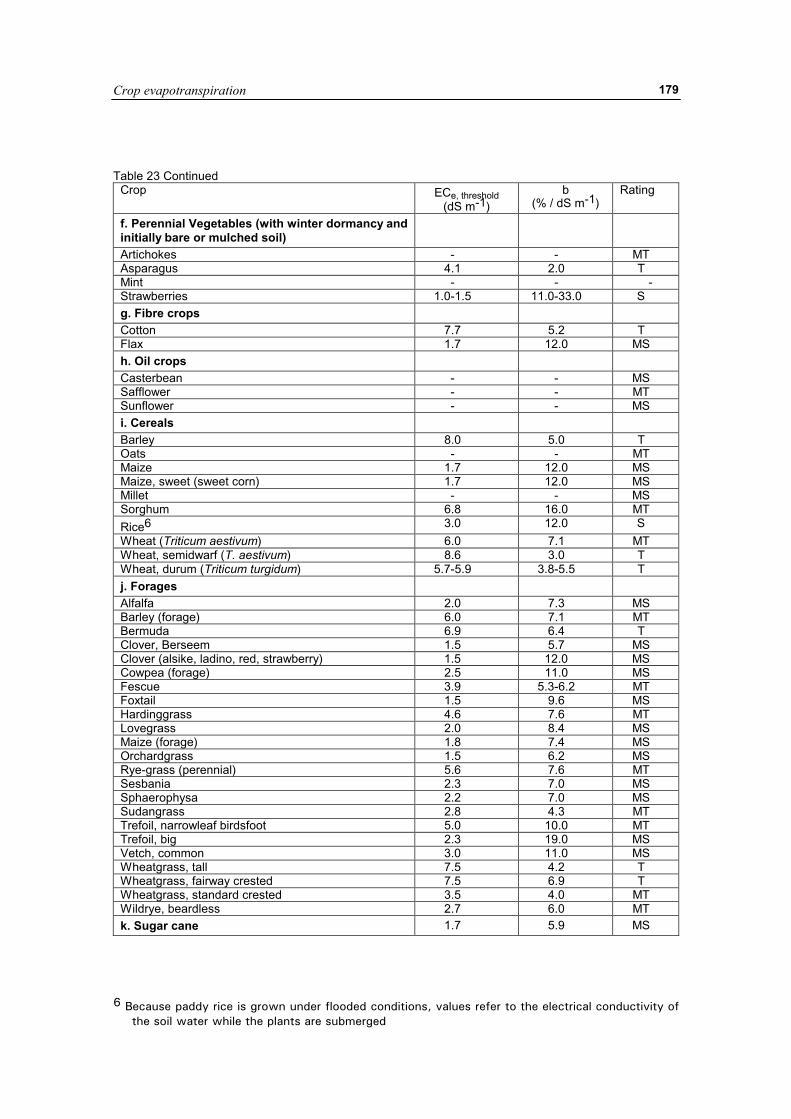
Crop evapotranspiration
179
Table 23 Continued Crop ECe, threshold
(dS m-1) b
(% / dS m-1) Rating
f. Perennial Vegetables (with winter dormancy and initially bare or mulched soil)
Artichokes - - MT Asparagus 4.1 2.0 T Mint - - - Strawberries 1.0-1.5 11.0-33.0 S g. Fibre crops Cotton 7.7 5.2 T Flax 1.7 12.0 MS h. Oil crops Casterbean - - MS Safflower - - MT Sunflower - - MS i. Cereals Barley 8.0 5.0 T Oats - - MT Maize 1.7 12.0 MS Maize, sweet (sweet corn) 1.7 12.0 MS Millet - - MS Sorghum 6.8 16.0 MT Rice6 3.0 12.0 S Wheat (Triticum aestivum) 6.0 7.1 MT Wheat, semidwarf (T. aestivum) 8.6 3.0 T Wheat, durum (Triticum turgidum) 5.7-5.9 3.8-5.5 T j. Forages Alfalfa 2.0 7.3 MS Barley (forage) 6.0 7.1 MT Bermuda 6.9 6.4 T Clover, Berseem 1.5 5.7 MS Clover (alsike, ladino, red, strawberry) 1.5 12.0 MS Cowpea (forage) 2.5 11.0 MS Fescue 3.9 5.3-6.2 MT Foxtail 1.5 9.6 MS Hardinggrass 4.6 7.6 MT Lovegrass 2.0 8.4 MS Maize (forage) 1.8 7.4 MS Orchardgrass 1.5 6.2 MS Rye-grass (perennial) 5.6 7.6 MT Sesbania 2.3 7.0 MS Sphaerophysa 2.2 7.0 MS Sudangrass 2.8 4.3 MT Trefoil, narrowleaf birdsfoot 5.0 10.0 MT Trefoil, big 2.3 19.0 MS Vetch, common 3.0 11.0 MS Wheatgrass, tall 7.5 4.2 T Wheatgrass, fairway crested 7.5 6.9 T Wheatgrass, standard crested 3.5 4.0 MT Wildrye, beardless 2.7 6.0 MT k. Sugar cane 1.7 5.9 MS
6 Because paddy rice is grown under flooded conditions, values refer to the electrical conductivity of
the soil water while the plants are submerged
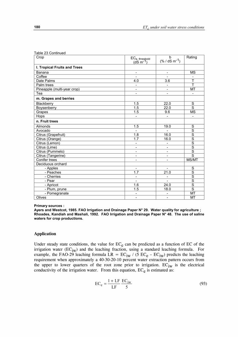
ETc under soil water stress conditions
180
Table 23 Continued Crop ECe, threshold
(dS m-1) b
(% / dS m-1) Rating
l. Tropical Fruits and Trees Banana - - MS Coffee - - - Date Palms 4.0 3.6 T Palm trees - - T Pineapple (multi-year crop) - - MT Tea - - - m. Grapes and berries Blackberry 1.5 22.0 S Boysenberry 1.5 22.0 S Grapes 1.5 9.6 MS Hops - - - n. Fruit trees Almonds 1.5 19.0 S Avocado - - S Citrus (Grapefruit) 1.8 16.0 S Citrus (Orange) 1.7 16.0 S Citrus (Lemon) - - S Citrus (Lime) - - S Citrus (Pummelo) - - S Citrus (Tangerine) - - S Conifer trees - - MS/MT Deciduous orchard - Apples - - S - Peaches 1.7 21.0 S - Cherries - - S - Pear - - S - Apricot 1.6 24.0 S - Plum, prune 1.5 18.0 S - Pomegranate - - MT Olives - - MT
Primary sources : Ayers and Westcot, 1985. FAO Irrigation and Drainage Paper N° 29. Water quality for agriculture ; Rhoades, Kandiah and Mashali, 1992. FAO Irrigation and Drainage Paper N° 48. The use of saline waters for crop productions. Application Under steady state conditions, the value for ECe can be predicted as a function of EC of the irrigation water (ECiw) and the leaching fraction, using a standard leaching formula. For example, the FAO-29 leaching formula LR = ECiw / (5 ECe – ECiw) predicts the leaching requirement when approximately a 40-30-20-10 percent water extraction pattern occurs from the upper to lower quarters of the root zone prior to irrigation. ECiw is the electrical conductivity of the irrigation water. From this equation, ECe is estimated as:
5
ECLF
LF1EC iwe
+= (93)
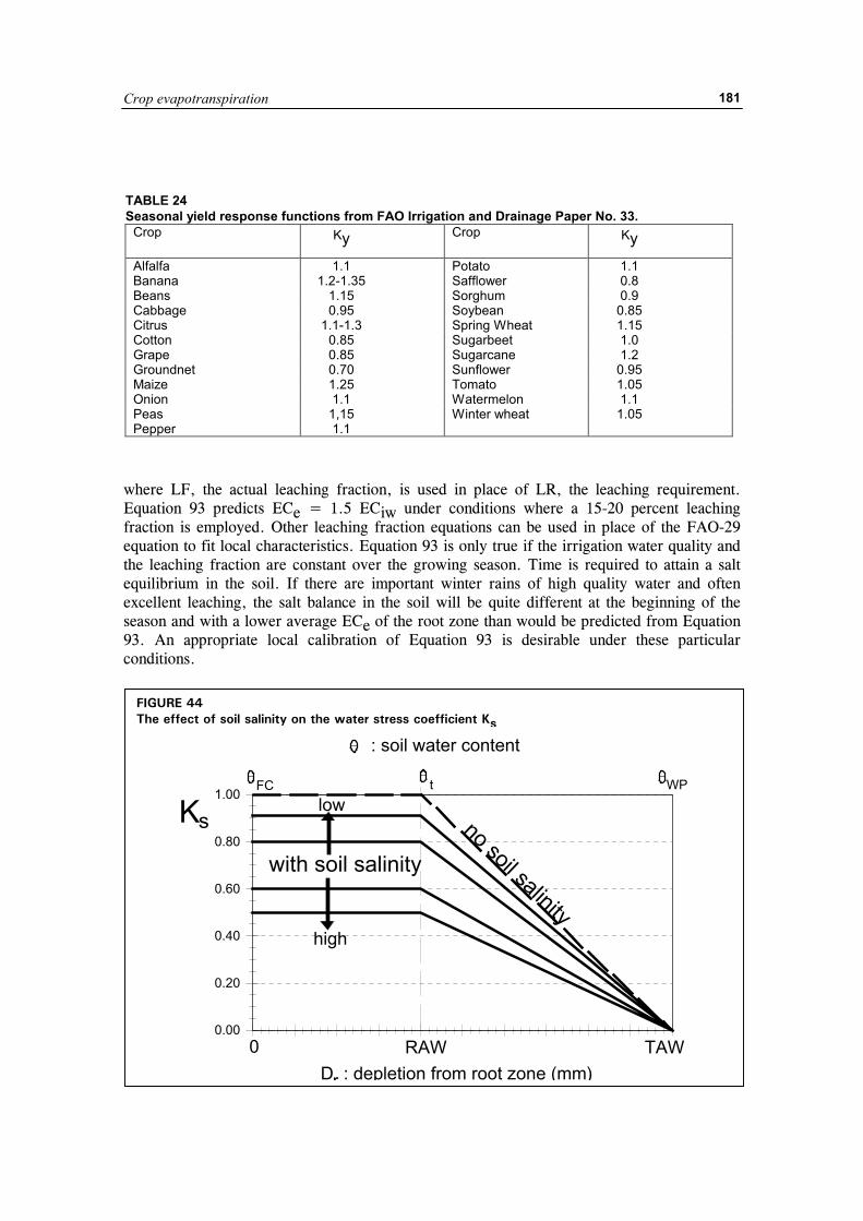
Crop evapotranspiration
181
where LF, the actual leaching fraction, is used in place of LR, the leaching requirement. Equation 93 predicts ECe = 1.5 ECiw under conditions where a 15-20 percent leaching fraction is employed. Other leaching fraction equations can be used in place of the FAO-29 equation to fit local characteristics. Equation 93 is only true if the irrigation water quality and the leaching fraction are constant over the growing season. Time is required to attain a salt equilibrium in the soil. If there are important winter rains of high quality water and often excellent leaching, the salt balance in the soil will be quite different at the beginning of the season and with a lower average ECe of the root zone than would be predicted from Equation 93. An appropriate local calibration of Equation 93 is desirable under these particular conditions.
TABLE 24 Seasonal yield response functions from FAO Irrigation and Drainage Paper No. 33.
Crop Ky
Crop Ky
Alfalfa 1.1 Potato 1.1 Banana 1.2-1.35 Safflower 0.8 Beans 1.15 Sorghum 0.9 Cabbage 0.95 Soybean 0.85 Citrus 1.1-1.3 Spring Wheat 1.15 Cotton 0.85 Sugarbeet 1.0 Grape 0.85 Sugarcane 1.2 Groundnet 0.70 Sunflower 0.95 Maize 1.25 Tomato 1.05 Onion 1.1 Watermelon 1.1 Peas 1,15 Winter wheat 1.05 Pepper 1.1
FIGURE 44 The effect of soil salinity on the water stress coefficient Ks
0.00
0.20
0.40
0.60
0.80
1.00
: soil water content
FC t WP
D : depletion from root zone (mm)r
Ks
0 RAW TAW
low
high
with soil salinity
no soil salinity
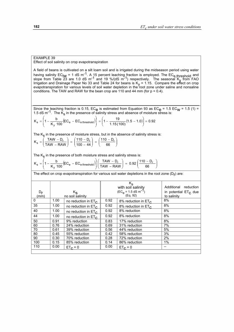
ETc under soil water stress conditions
182
EXAMPLE 39 Effect of soil salinity on crop evapotranspiration A field of beans is cultivated on a silt loam soil and is irrigated during the midseason period using water having salinity ECiw = 1 dS m-1. A 15 percent leaching fraction is employed. The ECe,threshold and slope from Table 23 are 1.0 dS m-1 and 19 %/(dS m-1) respectively. The seasonal Ky from FAO Irrigation and Drainage Paper No 33 and Table 24 for beans is Ky = 1.15. Compare the effect on crop evapotranspiration for various levels of soil water depletion in the root zone under saline and nonsaline conditions. The TAW and RAW for the bean crop are 110 and 44 mm (for p = 0.4).
Since the leaching fraction is 0.15, ECe is estimated from Equation 93 as ECe = 1.5 ECw = 1.5 (1) = 1.5 dS m-1. The Ks in the presence of salinity stress and absence of moisture stress is:
( ) ( ) 92.00.15.1)100(15.1
191ECEC100Kb1K thresholdee
ys =��
�
����
�−−=
��
�
�
��
�
�−−=
The Ks in the presence of moisture stress, but in the absence of salinity stress is:
���
����
� −=��
�
����
�
−−
=���
����
�
−−
=66
D11044100D110
RAWTAWDTAWK rrr
s
The Ks in the presence of both moisture stress and salinity stress is:
( ) ���
����
� −=��
�
����
�
−−
��
�
�
��
�
�−−=
66D11092.0
RAWTAWDTAWECEC
100Kb1K rr
thresholdeey
s
The effect on crop evapotranspiration for various soil water depletions in the root zone (Dr) are:
Dr (mm)
Ks no soil salinity
Ks with soil salinity (ECe = 1.5 dS m-1)
(Eq. 92)
Additional reduction in potential ETc due to salinity
0 1.00 no reduction in ETc 0.92 8% reduction in ETc 8% 35 1.00 no reduction in ETc 0.92 8% reduction in ETc 8% 40 1.00 no reduction in ETc 0.92 8% reduction 8% 44 1.00 no reduction in ETc 0.92 8% reduction 8% 50 0.91 9% reduction 0.83 17% reduction 8% 60 0.76 24% reduction 0.69 31% reduction 7% 70 0.61 39% reduction 0.56 44% reduction 5% 80 0.45 55% reduction 0.42 58% reduction 3% 90 0.30 70% reduction 0.28 72% reduction 2% 100 0.15 85% reduction 0.14 86% reduction 1% 110 0.00 ETc = 0 0.00 ETc = 0 --
Crop evapotranspiration
183
Chapter 9
ETc for natural, non-typical and non-pristine vegetation
Non-typical refers to types or arrangements of agricultural crops that are not listed or described in Tables 12 and 17. Non-pristine vegetation is defined, in the usage here, as vegetation having less than perfect growing conditions or stand characteristics (i.e., relatively poorer conditions of density, height, leaf area, fertility, or vitality) as compared to ‘pristine’ conditions.
The approach whereby a crop is characterized by a crop coefficient, Kc, and the crop evapotranspiration is given by the product of Kc and the reference evapotranspiration ETo, provides a simple and convenient way of also characterizing the evapotranspiration from natural vegetation and for non-typical cultivation practices. This chapter presents procedures for estimating Kc values for natural vegetation and for agricultural vegetation for which Kc values are not available. CALCULATION APPROACH
As described in Figure 27, the first step in the KcETo approach is the estimation of lengths of growth stages. This also applies to natural and other vegetation. The next step is the development of crop coefficient curves that represent the ratios of ETc to ETo during the various growth stages of the vegetation. Initial growth stage
The procedure to estimate crop coefficients for the initial growth stage for natural, non-typical and non-pristine vegetation is identical to that described in Chapter 6 (single crop coefficient Kc ini) or Chapter 7 (dual crop coefficient, Kcb ini + Ke). The crop coefficient in this stage is primarily determined by the frequency with which the soil is wetted. Mid and late season stages
The Kc during the mid-season period (Kc mid and Kcb mid) and to a lesser extent the Kc during the late season period differ from that described in previous chapters. As the ground cover for natural and non-pristine vegetation is often reduced, the Kc is affected to a large extent by the frequency of precipitation and/or irrigation and by the amount of leaf area and ground cover. Dual crop coefficient approach
The determination of Kc for natural, non-typical or non-pristine vegetation should ordinarily follow the approach described in Chapter 7 whereby separate transpiration (Kcb) and evaporation (Ke) coefficients are used. The effects of evaporation from the soil surface can be directly estimated as such.
ETc for natural, non-typical and non-pristine vegetation
184
Two procedures that can be used to adjust the basal crop coefficient (Kcb mid adj) for sparse vegetation are presented in this section. In these approaches, Kcb mid adj is estimated either from LAI (Equation 97) or from effective ground cover (Equation 98). After the determination of Kcb mid adj, the soil evaporation coefficient, Ke, should be determined to obtain the crop coefficient for the mid-season stage: Kc mid adj = Kcb mid adj + Ke. Procedures for calculating Ke are presented in Chapter 7.
Even where the estimated Kcb mid adj is small, the total Kc adj (= Kcb adj + Ke) following precipitation may sometimes be as high or higher than the Kc for pristine vegetation due to surface evaporation from among sparse vegetation. Single crop coefficient approach
When the single crop coefficient Kc of Chapter 6 is used, the average effects of soil wetting are incorporated into a general mean Kc. Some guidelines for the estimation of Kc adj are given in the following sections. The single crop coefficient can also be derived from the adjusted Kcb by considering the frequency of soil wetting, i.e., during the midseason period, Kc adj = Kcb adj + 0.05 for infrequent wetting and Kcb adj + 0.10 for wettings of up to once a week. For more frequent wettings, the dual crop coefficient approach should be used.
Alternatively, Equations 97 and 98 can be used to determine Kc instead of Kcb. Then, Kc min in Equations 97 and 98 can be set equal to Kc ini, where Kc ini is estimated from Figure 29 or 30. The use of Kc ini incorporates effects of soil evaporation and therefore serves as a lower limit on the estimate for Kc mid. Water stress conditions
Where rainfall or irrigation is low, water stress might be induced and the evapotranspiration will drop below the standard crop evapotranspiration, ETc. The reduction in the value for Kc under conditions of low soil water availability is determined using the stress coefficient Ks as described in Chapter 8. MID-SEASON STAGE - ADJUSTMENT FOR SPARSE VEGETATION
Adjustment from simple field observations
As a rough approximation for Kc during the mid-season stage for crops that usually nearly completely shade the soil under pristine conditions, but where cover is reduced due to disease, stress, pests, or planting density, the values for Kc mid and Kcb mid can be reduced by a factor depending on the actual vegetation development:
cmcdjac AKK −= (94) where Kc the Kc from Table 12 (Kc mid) or 17 (Kcb mid) after adjusting it for
climate (Equation 62 or 70), Kc adj the adjusted Kc (Kc mid adj or Kcb mid adj).
The Kc adjustment using Equation 94 does not apply when crops are frequently wetted and increased soil evaporation compensates for the reduced ground cover. Under these conditions Equation 94 should be applied only to Kcb.
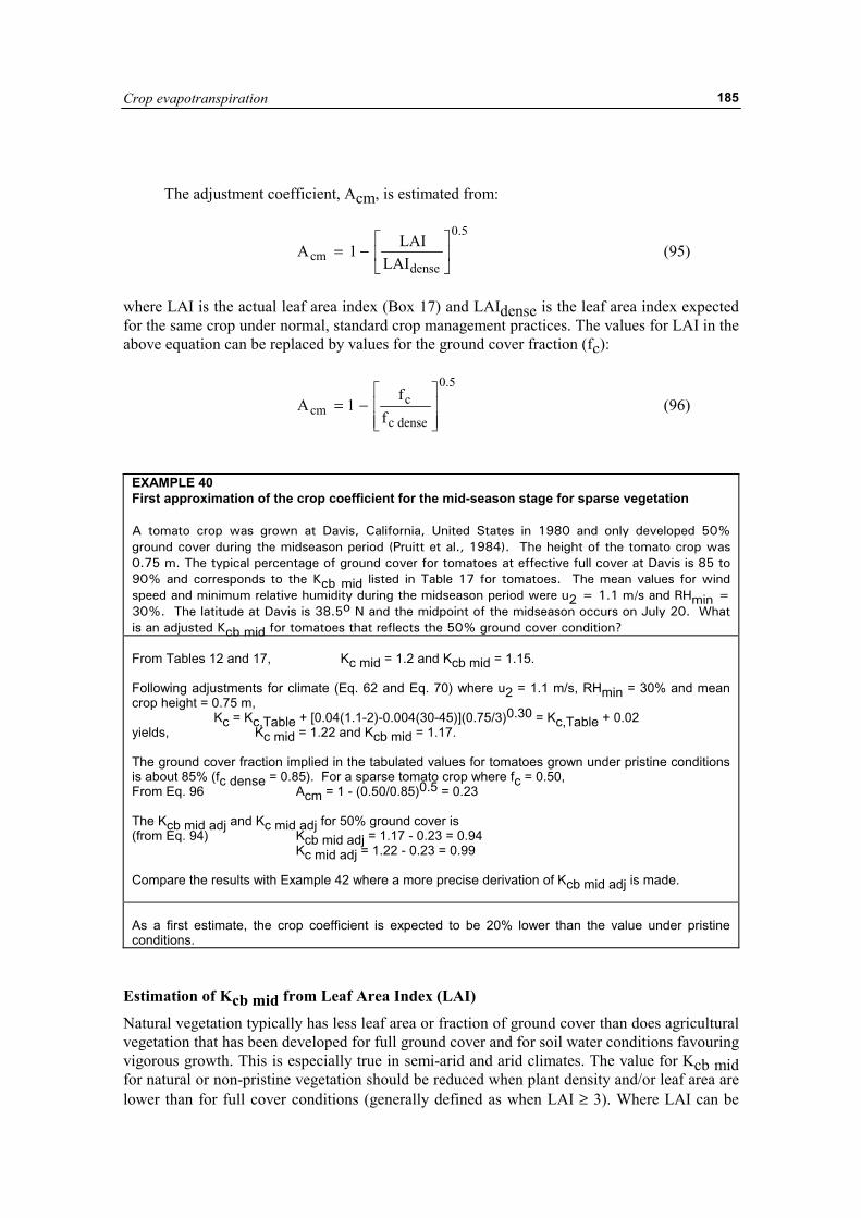
Crop evapotranspiration
185
The adjustment coefficient, Acm, is estimated from:
5.0
densecm LAI
LAI1A ��
���
�−= (95)
where LAI is the actual leaf area index (Box 17) and LAIdense is the leaf area index expected for the same crop under normal, standard crop management practices. The values for LAI in the above equation can be replaced by values for the ground cover fraction (fc):
5.0
densec
ccm f
f1A
���
�
���
�−= (96)
EXAMPLE 40 First approximation of the crop coefficient for the mid-season stage for sparse vegetation A tomato crop was grown at Davis, California, United States in 1980 and only developed 50% ground cover during the midseason period (Pruitt et al., 1984). The height of the tomato crop was 0.75 m. The typical percentage of ground cover for tomatoes at effective full cover at Davis is 85 to 90% and corresponds to the Kcb mid listed in Table 17 for tomatoes. The mean values for wind speed and minimum relative humidity during the midseason period were u2 = 1.1 m/s and RHmin = 30%. The latitude at Davis is 38.5o N and the midpoint of the midseason occurs on July 20. What is an adjusted Kcb mid for tomatoes that reflects the 50% ground cover condition? From Tables 12 and 17, Kc mid = 1.2 and Kcb mid = 1.15. Following adjustments for climate (Eq. 62 and Eq. 70) where u2 = 1.1 m/s, RHmin = 30% and mean crop height = 0.75 m, Kc = Kc,Table + [0.04(1.1-2)-0.004(30-45)](0.75/3)0.30 = Kc,Table + 0.02 yields, Kc mid = 1.22 and Kcb mid = 1.17. The ground cover fraction implied in the tabulated values for tomatoes grown under pristine conditions is about 85% (fc dense = 0.85). For a sparse tomato crop where fc = 0.50, From Eq. 96 Acm = 1 - (0.50/0.85)0.5 = 0.23 The Kcb mid adj and Kc mid adj for 50% ground cover is (from Eq. 94) Kcb mid adj = 1.17 - 0.23 = 0.94 Kc mid adj = 1.22 - 0.23 = 0.99 Compare the results with Example 42 where a more precise derivation of Kcb mid adj is made. As a first estimate, the crop coefficient is expected to be 20% lower than the value under pristine conditions.
Estimation of Kcb mid from Leaf Area Index (LAI)
Natural vegetation typically has less leaf area or fraction of ground cover than does agricultural vegetation that has been developed for full ground cover and for soil water conditions favouring vigorous growth. This is especially true in semi-arid and arid climates. The value for Kcb mid for natural or non-pristine vegetation should be reduced when plant density and/or leaf area are lower than for full cover conditions (generally defined as when LAI ≥ 3). Where LAI can be
ETc for natural, non-typical and non-pristine vegetation
186
measured or approximated, a peak Kcb mid for natural, non-typical or non-pristine agricultural vegetation can be approximated similar to a procedure used by Ritchie as:
( )( )]LAI7.0[exp1KKKK mincfullcbmincmidcb −−−+= (97)
where Kcb mid estimated basal Kcb during the mid-season when plant density and/or leaf area are lower than for full cover conditions,
Kcb full estimated basal Kcb during the mid-season (at peak plant size or height) for vegetation having full ground cover or LAI > 3 (Equations 99 and 100),
Kc min the minimum Kc for bare soil (Kc min ≈ 0.15 - 0.20), LAI actual leaf area index, defined as the area of leaves per area of
underlying ground surface averaged over a large area. Only one side of leaves is counted [m2 m-2].
Equation 97 is recommended for annual types of vegetation that are either natural or are
in a non-pristine state due to sparse density or effects of some type of environmental stress on growth.
The relationship expressed in Equation 97 produces results similar to those suggested by Ritchie (1974). For LAI > 3, Kcb mid ≈ Kcb full. The LAI used in Equation 97 should be the ‘green’ LAI representing only healthy leaves that are active in vapour transfer.
BOX 17 Measuring and estimating LAI LAI can be measured directly by harvesting all green healthy leaves from vegetation over a measured or prescribed area, for example, 1 m2 or 10 m2, and then measuring and summing the areas of individual leaves using photometric methods or by measuring areas of several representative leaves, averaging, and then multiplying by the total number of leaves counted. In the absence of measurements for LAI, LAI can be estimated for sparse, annual vegetation as:
a
densedense Population
PopulationLAILAI ��
���
�=
where LAIdense LAI for the particular plant species under normal, ‘dense’ or pristine
growing conditions. LAIdense can be obtained from various physiological sources and textbooks on crops and vegetation.
Population number of plants per unit area of soil surface under the actual growing conditions [No. m-2].
Populationdense number of plants per unit area of soil surface under the ‘dense’ or pristine growing conditions [No. m-2]. a a = 0.5 when population is formed from vigorous growing plants; a
= 1 when plants are less vigorous.
The 0.5 exponent in the equation simulates the tendency for vegetation to compensate for reduced stand density by increasing the size and total leaf areas for individual plants. Therefore, LAI does not fall in direct proportion to plant population. Under conditions where the plant size does not increase with reduced stand density, the ’a’ exponent in the equation should be set to 1 (a = 1). These latter conditions may occur where soil fertility is poor or where soil salinity, soil water stress, or waterlogging inhibit both growth and stand density, so that the growth of individual plants is retarded.
Crop evapotranspiration
187
Estimation of Kcb mid from effective ground cover (fc eff) Where only estimates of the fraction of soil surface effectively covered by vegetation are available, the following approximation for Kcb mid adj can be used:
( ) ( )����
�
�
����
�
�
����
�
�
����
�
�
−+=���
����
�
+ h11
effccmincfullcbmincmidcb f,f2,1minKKKK (98)
where Kcb mid estimated basal Kcb during the mid-season when plant density and/or
leaf area are lower than for full cover conditions, Kcb full estimated basal Kcb during the mid-season (at peak plant size or height)
for vegetation having full ground cover or LAI > 3 (see Equations 99 and 100),
Kc min the minimum Kc for bare soil (in the presence of vegetation) (Kc min ≈ 0.15 - 0.20),
fc observed fraction of soil surface that is covered by vegetation as observed from nadir (overhead) [0.01 - 1],
fc eff the effective fraction of soil surface covered or shaded by vegetation [0.01-1] (see Box 18),
h the plant height [m].
Stomatal conductance and water transport within plants may limit ET under conditions of sparse, tall vegetation. Under these conditions, Kcb mid is limited by the “2fc” term in Equation 98. Equation 98 applies well to trees and shrubs.
BOX 18 Measuring and estimating fc eff fc eff should normally represent the fraction of the soil surface that is shaded by vegetation. This value is generally larger than fc, the actual fraction of the soil surface that is covered by vegetation as observed from directly overhead. The amount of shading represents the amount of solar radiation intercepted by plants for potential conversion into evapotranspiration. The total fraction of shading is a function of the sun angle and the horizontal size and shape of individual plants (or rows) relative to their height. fc eff for ‘rectangular’ shaped canopies such as most agricultural plant rows can be approximated as:
1)tan(
HWR1ff ceffc ≤��
���
�
η+=
where fc observed fraction of soil surface that is covered by vegetation as observed from nadir
(overhead) [0.01 - 1], HWR height to width ratio of individual plants or groups of plants when viewed from the east
or from the west [ ], tan(η) tangent of the mean angle of the sun, η, above the horizon during the period of
maximum evapotranspiration (generally between 11.00 and 15.00 hours) [ ]. For most applications, η can be computed at solar noon (12.00 hours).
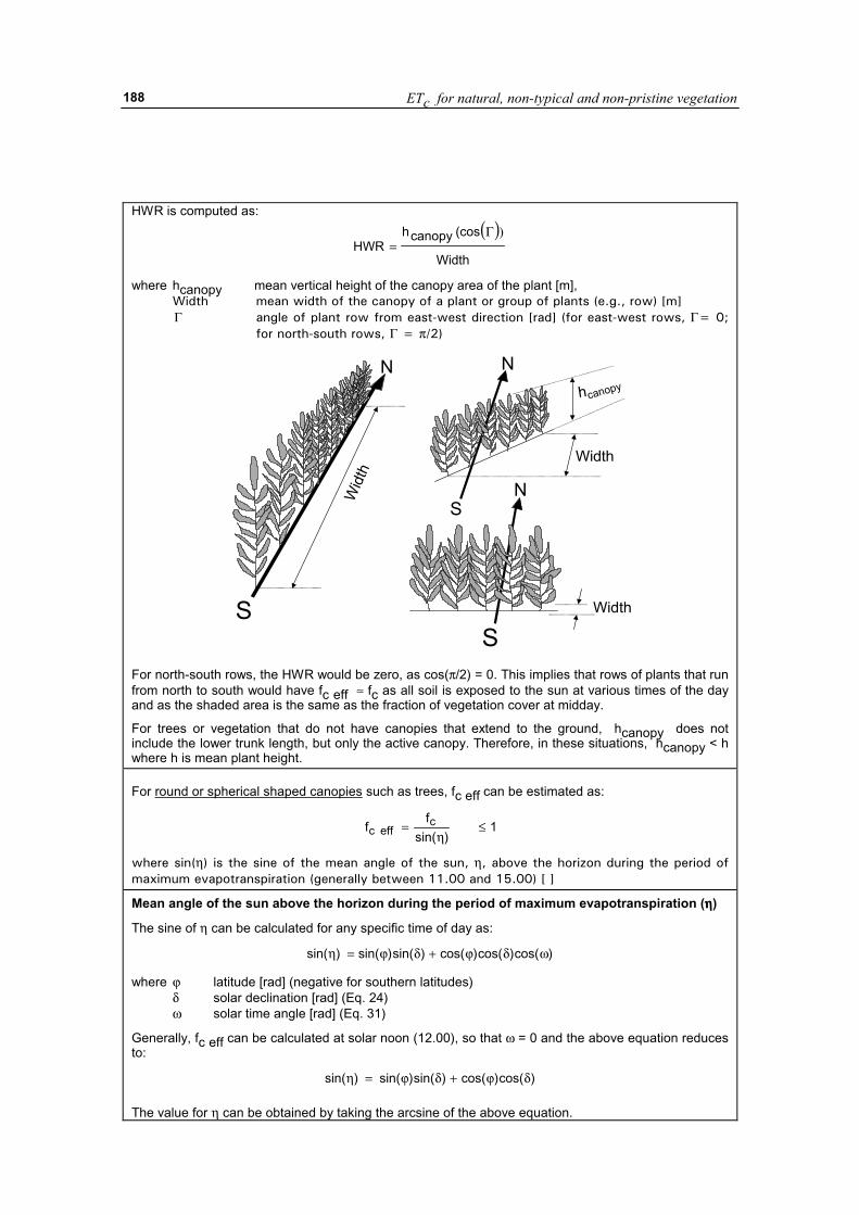
ETc for natural, non-typical and non-pristine vegetation
188
HWR is computed as:
( )Width
(coscanopyhHWR
)Γ=
where hcanopy mean vertical height of the canopy area of the plant [m], Width mean width of the canopy of a plant or group of plants (e.g., row) [m] Γ angle of plant row from east-west direction [rad] (for east-west rows, Γ= 0;
for north-south rows, Γ = π/2)
S S
N N
N Wid
th
Width
Width
S
hcanopy
For north-south rows, the HWR would be zero, as cos(π/2) = 0. This implies that rows of plants that run from north to south would have fc eff ≈ fc as all soil is exposed to the sun at various times of the day and as the shaded area is the same as the fraction of vegetation cover at midday.
For trees or vegetation that do not have canopies that extend to the ground, hcanopy does not include the lower trunk length, but only the active canopy. Therefore, in these situations, hcanopy < h where h is mean plant height. For round or spherical shaped canopies such as trees, fc eff can be estimated as:
1)sin(
ff c
effc ≤η
=
where sin(η) is the sine of the mean angle of the sun, η, above the horizon during the period of maximum evapotranspiration (generally between 11.00 and 15.00) [ ]
Mean angle of the sun above the horizon during the period of maximum evapotranspiration (ηηηη)
The sine of η can be calculated for any specific time of day as:
)cos()cos()cos()sin()sin()sin( ωδϕ+δϕ=η
where ϕ latitude [rad] (negative for southern latitudes) δ solar declination [rad] (Eq. 24) ω solar time angle [rad] (Eq. 31)
Generally, fc eff can be calculated at solar noon (12.00), so that ω = 0 and the above equation reduces to:
)cos()cos()sin()sin()sin( δϕ+δϕ=η The value for η can be obtained by taking the arcsine of the above equation.
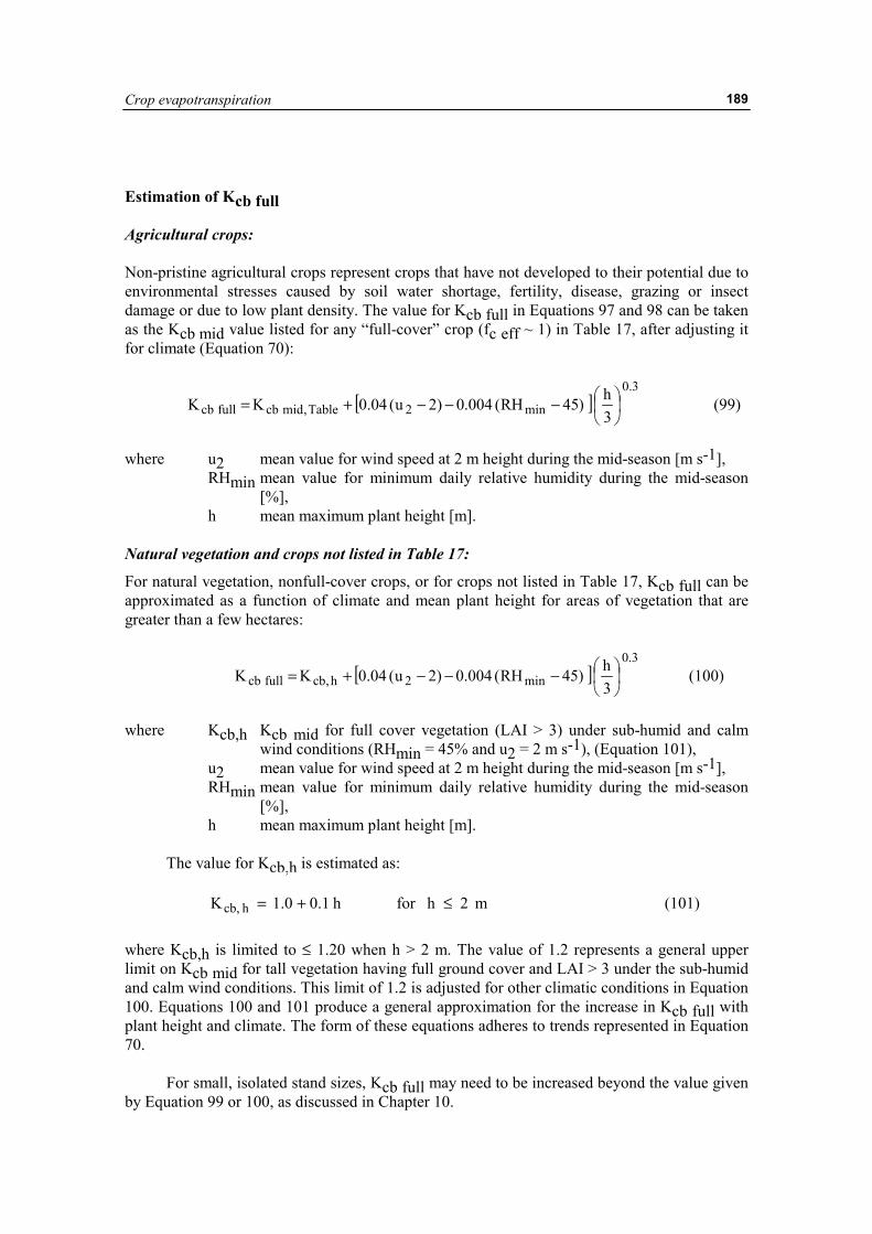
Crop evapotranspiration
189
Estimation of Kcb full Agricultural crops: Non-pristine agricultural crops represent crops that have not developed to their potential due to environmental stresses caused by soil water shortage, fertility, disease, grazing or insect damage or due to low plant density. The value for Kcb full in Equations 97 and 98 can be taken as the Kcb mid value listed for any “full-cover” crop (fc eff ~ 1) in Table 17, after adjusting it for climate (Equation 70):
[ ]3.0
min2Table,midcbfullcb 3h)45RH(004.0)2u(04.0KK ��
���
�−−−+= (99)
where u2 mean value for wind speed at 2 m height during the mid-season [m s-1],
RHmin mean value for minimum daily relative humidity during the mid-season [%],
h mean maximum plant height [m]. Natural vegetation and crops not listed in Table 17:
For natural vegetation, nonfull-cover crops, or for crops not listed in Table 17, Kcb full can be approximated as a function of climate and mean plant height for areas of vegetation that are greater than a few hectares:
[ ]3.0
min2h,cbfullcb 3h)45RH(004.0)2u(04.0KK ��
���
�−−−+= (100)
where Kcb,h Kcb mid for full cover vegetation (LAI > 3) under sub-humid and calm
wind conditions (RHmin = 45% and u2 = 2 m s-1), (Equation 101), u2 mean value for wind speed at 2 m height during the mid-season [m s-1], RHmin mean value for minimum daily relative humidity during the mid-season
[%], h mean maximum plant height [m].
The value for Kcb,h is estimated as:
m2hforh1.00.1K h,cb ≤+= (101) where Kcb,h is limited to ≤ 1.20 when h > 2 m. The value of 1.2 represents a general upper limit on Kcb mid for tall vegetation having full ground cover and LAI > 3 under the sub-humid and calm wind conditions. This limit of 1.2 is adjusted for other climatic conditions in Equation 100. Equations 100 and 101 produce a general approximation for the increase in Kcb full with plant height and climate. The form of these equations adheres to trends represented in Equation 70.
For small, isolated stand sizes, Kcb full may need to be increased beyond the value given by Equation 99 or 100, as discussed in Chapter 10.
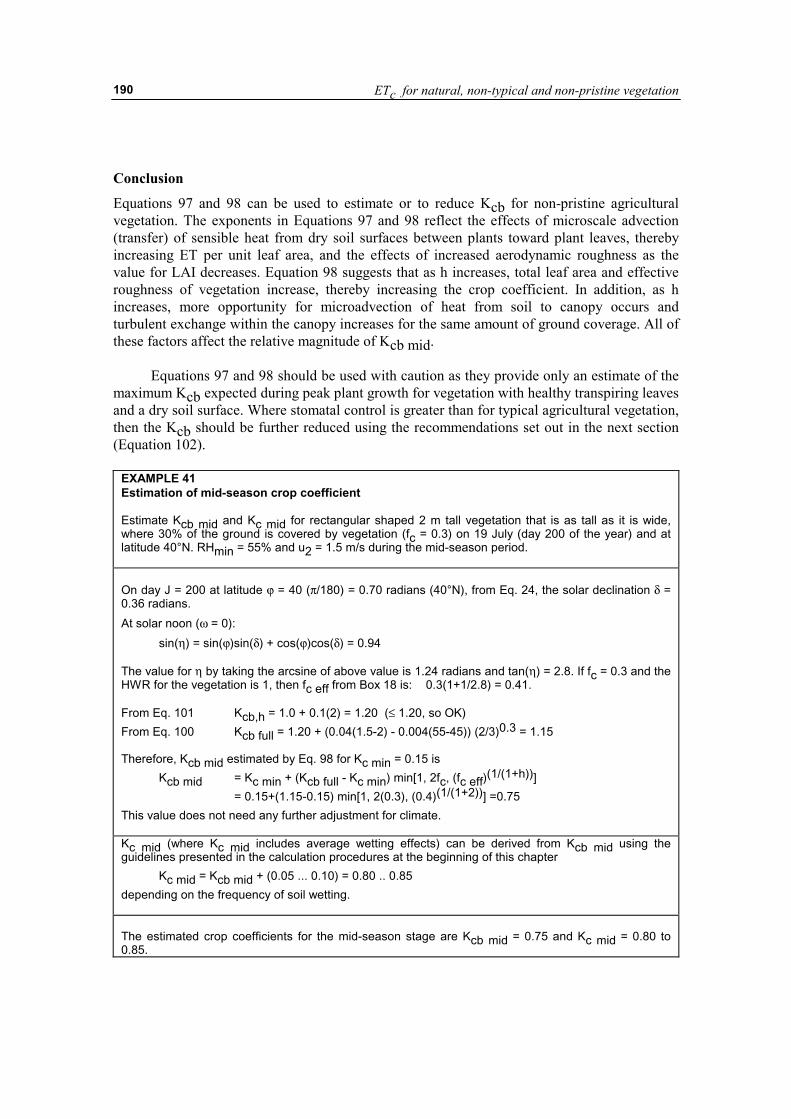
ETc for natural, non-typical and non-pristine vegetation
190
Conclusion
Equations 97 and 98 can be used to estimate or to reduce Kcb for non-pristine agricultural vegetation. The exponents in Equations 97 and 98 reflect the effects of microscale advection (transfer) of sensible heat from dry soil surfaces between plants toward plant leaves, thereby increasing ET per unit leaf area, and the effects of increased aerodynamic roughness as the value for LAI decreases. Equation 98 suggests that as h increases, total leaf area and effective roughness of vegetation increase, thereby increasing the crop coefficient. In addition, as h increases, more opportunity for microadvection of heat from soil to canopy occurs and turbulent exchange within the canopy increases for the same amount of ground coverage. All of these factors affect the relative magnitude of Kcb mid.
Equations 97 and 98 should be used with caution as they provide only an estimate of the maximum Kcb expected during peak plant growth for vegetation with healthy transpiring leaves and a dry soil surface. Where stomatal control is greater than for typical agricultural vegetation, then the Kcb should be further reduced using the recommendations set out in the next section (Equation 102).
EXAMPLE 41 Estimation of mid-season crop coefficient Estimate Kcb mid and Kc mid for rectangular shaped 2 m tall vegetation that is as tall as it is wide, where 30% of the ground is covered by vegetation (fc = 0.3) on 19 July (day 200 of the year) and at latitude 40°N. RHmin = 55% and u2 = 1.5 m/s during the mid-season period. On day J = 200 at latitude ϕ = 40 (π/180) = 0.70 radians (40°N), from Eq. 24, the solar declination δ = 0.36 radians. At solar noon (ω = 0): sin(η) = sin(ϕ)sin(δ) + cos(ϕ)cos(δ) = 0.94 The value for η by taking the arcsine of above value is 1.24 radians and tan(η) = 2.8. If fc = 0.3 and the HWR for the vegetation is 1, then fc eff from Box 18 is: 0.3(1+1/2.8) = 0.41. From Eq. 101 Kcb,h = 1.0 + 0.1(2) = 1.20 (≤ 1.20, so OK) From Eq. 100 Kcb full = 1.20 + (0.04(1.5-2) - 0.004(55-45)) (2/3)0.3 = 1.15 Therefore, Kcb mid estimated by Eq. 98 for Kc min = 0.15 is Kcb mid = Kc min + (Kcb full - Kc min) min[1, 2fc, (fc eff)(1/(1+h))] = 0.15+(1.15-0.15) min[1, 2(0.3), (0.4)(1/(1+2))] =0.75 This value does not need any further adjustment for climate. Kc mid (where Kc mid includes average wetting effects) can be derived from Kcb mid using the guidelines presented in the calculation procedures at the beginning of this chapter Kc mid = Kcb mid + (0.05 ... 0.10) = 0.80 .. 0.85 depending on the frequency of soil wetting. The estimated crop coefficients for the mid-season stage are Kcb mid = 0.75 and Kc mid = 0.80 to 0.85.
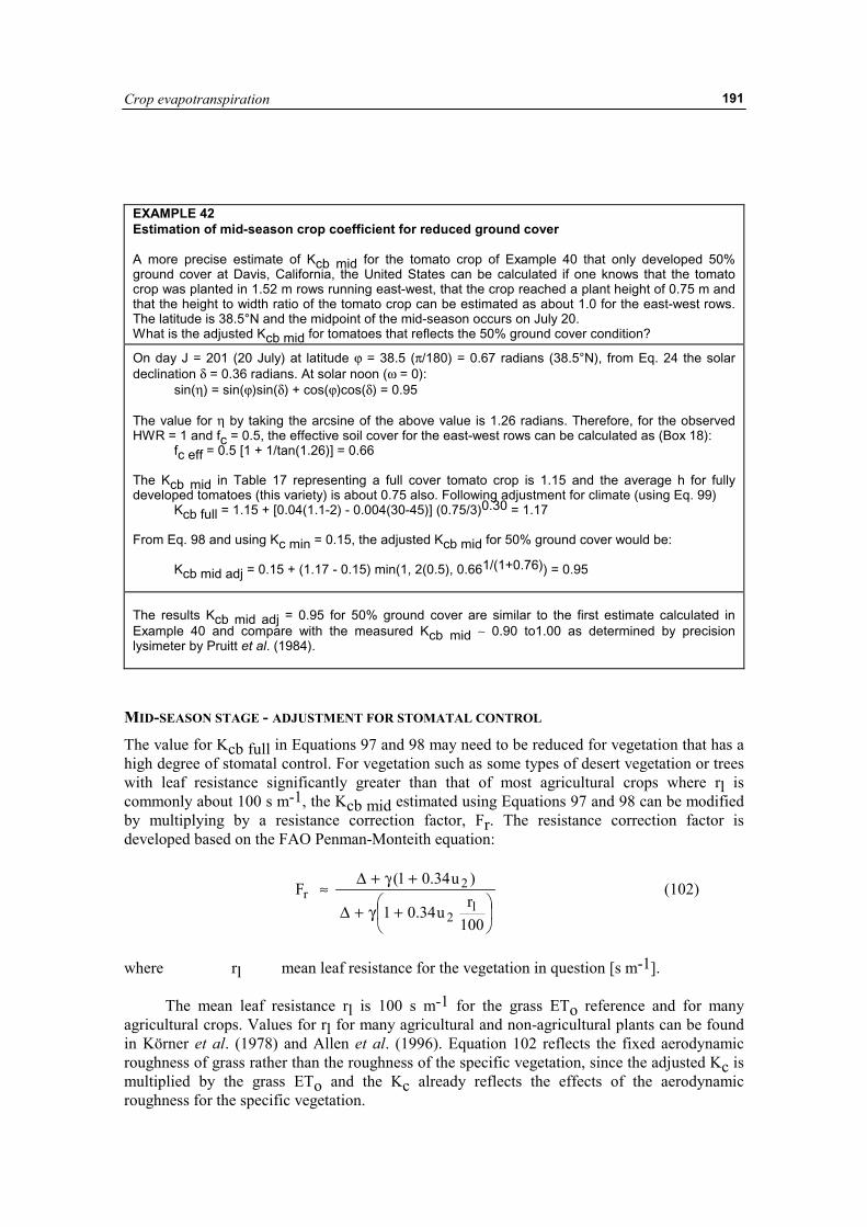
Crop evapotranspiration
191
EXAMPLE 42 Estimation of mid-season crop coefficient for reduced ground cover A more precise estimate of Kcb mid for the tomato crop of Example 40 that only developed 50% ground cover at Davis, California, the United States can be calculated if one knows that the tomato crop was planted in 1.52 m rows running east-west, that the crop reached a plant height of 0.75 m and that the height to width ratio of the tomato crop can be estimated as about 1.0 for the east-west rows. The latitude is 38.5°N and the midpoint of the mid-season occurs on July 20. What is the adjusted Kcb mid for tomatoes that reflects the 50% ground cover condition?
On day J = 201 (20 July) at latitude ϕ = 38.5 (π/180) = 0.67 radians (38.5°N), from Eq. 24 the solar declination δ = 0.36 radians. At solar noon (ω = 0): sin(η) = sin(ϕ)sin(δ) + cos(ϕ)cos(δ) = 0.95 The value for η by taking the arcsine of the above value is 1.26 radians. Therefore, for the observed HWR = 1 and fc = 0.5, the effective soil cover for the east-west rows can be calculated as (Box 18): fc eff = 0.5 [1 + 1/tan(1.26)] = 0.66 The Kcb mid in Table 17 representing a full cover tomato crop is 1.15 and the average h for fully developed tomatoes (this variety) is about 0.75 also. Following adjustment for climate (using Eq. 99) Kcb full = 1.15 + [0.04(1.1-2) - 0.004(30-45)] (0.75/3)0.30 = 1.17 From Eq. 98 and using Kc min = 0.15, the adjusted Kcb mid for 50% ground cover would be: Kcb mid adj = 0.15 + (1.17 - 0.15) min(1, 2(0.5), 0.661/(1+0.76)) = 0.95 The results Kcb mid adj = 0.95 for 50% ground cover are similar to the first estimate calculated in Example 40 and compare with the measured Kcb mid ∼ 0.90 to1.00 as determined by precision lysimeter by Pruitt et al. (1984).
MID-SEASON STAGE - ADJUSTMENT FOR STOMATAL CONTROL
The value for Kcb full in Equations 97 and 98 may need to be reduced for vegetation that has a high degree of stomatal control. For vegetation such as some types of desert vegetation or trees with leaf resistance significantly greater than that of most agricultural crops where rl is commonly about 100 s m-1, the Kcb mid estimated using Equations 97 and 98 can be modified by multiplying by a resistance correction factor, Fr. The resistance correction factor is developed based on the FAO Penman-Monteith equation:
��
���
� +γ+∆
+γ+∆≈
100r
u34.01
)u34.01(F
l2
2r (102)
where rl mean leaf resistance for the vegetation in question [s m-1].
The mean leaf resistance rl is 100 s m-1 for the grass ETo reference and for many agricultural crops. Values for rl for many agricultural and non-agricultural plants can be found in Körner et al. (1978) and Allen et al. (1996). Equation 102 reflects the fixed aerodynamic roughness of grass rather than the roughness of the specific vegetation, since the adjusted Kc is multiplied by the grass ETo and the Kc already reflects the effects of the aerodynamic roughness for the specific vegetation.
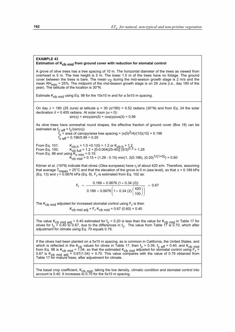
ETc for natural, non-typical and non-pristine vegetation
192
EXAMPLE 43 Estimation of Kcb mid from ground cover with reduction for stomatal control A grove of olive trees has a tree spacing of 10 m. The horizontal diameter of the trees as viewed from overhead is 5 m. The tree height is 5 m. The lower 1.5 m of the trees have no foliage. The ground cover between the trees is bare. The mean u2 during the mid-season growth stage is 2 m/s and the mean RHmin = 25%. The midpoint of the mid-season growth stage is on 29 June (i.e., day 180 of the year). The latitude of the location is 30°N. Estimate Kcb mid using Eq. 98 for the 10x10 m and for a 5x10 m spacing. On day J = 180 (29 June) at latitude ϕ = 30 (π/180) = 0.52 radians (30°N) and from Eq. 24 the solar declination δ = 0.405 radians. At solar noon (ω = 0): sin(η) = sin(ϕ)sin(δ) + cos(ϕ)cos(δ) = 0.99 As olive trees have somewhat round shapes, the effective fraction of ground cover (Box 18) can be estimated as fc eff = fc/(sin(η)). fc = area of canopy/area tree spacing = (π(5)2/4)/(10)(10) = 0.196 fc eff = 0.196/0.99 = 0.20 From Eq. 101: Kcb,h = 1.0 +0.1(5) > 1.2 or Kcb,h = 1.2 From Eq. 100: Kcb full = 1.2 + [0-0.004(25-45)] (5/3)0.3 = 1.29 From Eq. 98 and using Kc min = 0.15: Kcb mid = 0.15 + (1.29 - 0.15) min(1, 2(0.196), (0.20)1/(1+5)) = 0.60 Körner et al. (1979) indicate that olives (Olea europaea) have rl of about 420 s/m. Therefore, assuming that average Tmean = 25°C and that the elevation of the grove is 0 m (sea level), so that ∆ = 0.189 kPa (Eq. 13) and γ = 0.0676 kPa (Eq. 8), Fr is estimated from Eq. 102 as:
67.0
100420)2(34.010676.0189.0
))2(34.01(0676.0189.0Fr =
���
����
���
���
�++
++≈
The Kcb mid adjusted for increased stomatal control using Fr is then Kcb mid adj = Fr Kcb mid = 0.67 (0.60) = 0.40 The value Kcb mid adj = 0.40 estimated for fc = 0.20 is less than the value for Kcb mid in Table 17 for olives for fc = 0.40 to 0.67, due to the differences in fc. The value from Table 17 is 0.70, which after adjustment for climate using Eq. 70 equals 0.79. If the olives had been planted on a 5x10 m spacing, as is common in California, the United States, and which is reflected in the Kcb values for olives in Table 17, then fc = 0.39, fc eff = 0.40, and Kcb mid from Eq. 98 is Kcb mid = 1.04, so that the estimated Kcb mid adjusted for stomatal control using Fr = 0.67 is Kcb mid adj = 0.67(1.04) = 0.70. This value compares with the value of 0.79 obtained from Table 17 for mature trees, after adjustment for climate. The basal crop coefficient, Kcb mid, taking the low density, climatic condition and stomatal control into account is 0.40. It increases to 0.70 for the 5x10 m spacing.
Crop evapotranspiration
193
The equation would underestimate Fr (overestimate the reduction in Kcb) if used with the actual roughness of the vegetation when rl > 100 s m-1 because of the lack in Equation 102 of feedback effects that reduced ETc has on temperature and vapour pressure deficit profiles over the crop. These parameters generally increase with decreasing ETc and therefore dampen the reduction in ETc. LATE SEASON STAGE
During the late season stage, the Kcb begins to decrease until it reaches Kcb end at the end of the growing period. Values for Kcb end can be scaled from Kcb mid in proportion to the health and leaf condition of the vegetation at termination of the growing season and according to the length of the late season period (i.e., whether leaves senesce slowly or are killed by frost). Values for Kc end can be similarly scaled from Kc mid; however, the reduction in Kc end will be affected by the frequency of wetting by irrigation or precipitation and Kc end may be proportionally less.
If estimated from Equations 97 and 98, Kcb end should be reduced if it is to represent Kc values for plants with stomatal control that is greater than that for agricultural vegetation (where rl ≈ 100 s m-1) or to reflect effects of ageing and senescence on stomatal control. In these situations, the estimated Kcb end values should be multiplied by the Fr from Equation 102. Alternatively, they can be reduced by about 10% for each doubling of rl above 100 s m-1 when mean daily air temperature (Tmean) is about 30o C and by about 20% for each doubling of rl above 100 s m-1 when Tmean is about 15o C.
Alternatively, the value for Kcb end can be reduced relative to the calculated value for Kcb mid in proportion to the fraction of green healthy leaves remaining at the end of the late season stage relative to that during the mid-season. This can often be based on a visual survey of the field and may therefore be a subjective observation.
The fc parameter and h are probably the simplest indices to estimate in the field. Again, Equations 97 and 98 should be used only as general or preliminary estimates of Kcb end. ESTIMATING ETc adj USING CROP YIELDS A simple, linear crop-water production function was introduced in the FAO Irrigation and Drainage Paper No. 33 to predict the reduction in crop yield when crop stress is caused by a shortage of soil water. This function was presented earlier as Equation 90:
��
�
�
��
�
�−=��
�
����
�−
c
adjcy
m
aET
ET1K
YY
1 (90)
where Ya = actual yield of the crop [kg ha-1] Ym = maximum (expected) yield in absence of environmental or water
stresses Ky = yield response factor [ ] ETc = potential (expected) crop evapotranspiration in the absence of
environmental or water stresses (Kc ETo) ETc adj = actual (adjusted) crop evapotranspiration as a result of environmental
or water stresses
ETc for natural, non-typical and non-pristine vegetation
194
Values for Ky have been reported in Paper No. 33 for a wide range of crops for predicting the effect of water stress and associated reduction in ETc adj on crop yield. Factors are presented there for predicting yield reductions for when stress occurs in only one crop growth stage, or when stress is distributed throughout the growing period. Seasonal yield response functions are summarized in Table 24.
Many environmental stresses such as water shortage, salinity, low fertility and disease impact yield by reducing the amount of ETc adj relative to the potential amount ETc. The same can be true for when yields are reduced due to the use of low densities for plant populations. Therefore, for very general estimates of ETc adj, one can invert Equation 90 and solve for the stress factor, Ks:
���
����
�−−=
m
a
ys Y
Y1
K11K (103)
where Ks is multiplied by Kcb or by Kc in equations 80 or 81 to predict the ETc adj in the presense of the water or other environmental stresses or for low plant populations or virility. The ETc adj predicted using Ks from equation 103 provides only a very general and approximate estimate of monthly or even seasonal evapotranspiration. Equation 103 works best for forage or other indiscriminate crops where the value for Ky is relatively constant during the season.
Equation 103 is generally only valid for use in predicting actual crop evapotranspiration for use in regional water balance studies, for studies of ground-water depletion and recharge, or for estimating historical water use. The procedure is not valid for predicting ETc for daily or weekly time periods due to the very general nature of the Ky coefficient and the seasonal time scale of the crop yield. The procedures presented previously for adjusting ETc using a daily soil water balance, salinity functions, or reductions in Kc based on leaf area or fraction of ground cover are recommended over the use of equation 103.
EXAMPLE 44 Approximate estimation of Ks from crop yield data An irrigation scheme (project) cultivates dry, edible beans. There is known to be a shortage of irrigation water and a corresponding reduction in crop yield. The reported yield for the scheme averages 1100 kg/ha. The potential yield for the region and variety of beans, in the absence of water or environmental stresses and with good soil fertility is 1800 kg/ha. From FAO Irrigation and Drainage Paper No. 33 or Table 24, the Ky for dry beans, assuming that stresses are distributed uniformly through the growing season, is 1.15. Therefore, from Equation 103, the estimated Ks to apply with Equation 80 for the growing season is:
66.0180011001
15.111Ks =�
�
���
� −−=
Therefore, the ETc adj for the season is predicted to be only 0.66 of maximum ETc under pristine growing conditions.
The estimated seasonal ETc adj is predicted to be ETc adj = 0.66 ETc where ETc is predicted as ETc = Kc ETo.
Crop evapotranspiration
195
Chapter 10
ETc under various management practices
This chapter discusses various types of factors that may cause the values for Kc and ETc to deviate from the standard values described in the Chapters 6 and 7. These factors refer to the effects of surface mulches, intercropping, small areas of vegetation and specific cultivation practices.
This chapter is intended to serve as a resource for situations where cultivation practices are known to deviate from those assumed in Tables 12 and 17, but where estimates of Kc and ETc are still necessary. This chapter is by no means exhaustive. The intent is to demonstrate some of the procedures that can be used to make adjustments to Kc to account for deviations from standard conditions. EFFECTS OF SURFACE MULCHES Mulches are frequently used in vegetable production to reduce evaporation losses from the soil surface, to accelerate crop development in cool climates by increasing soil temperature, to reduce erosion, or to assist in weed control. Mulches may be composed of organic plant materials or they may be synthetic mulches consisting of plastic sheets. Plastic mulches Plastic mulches generally consist of thin sheets of polyethylene or a similar material placed over the ground surface, especially along the plant rows. Holes are cut into the plastic film at plant spacings to allow the plant vegetation to emerge. Plastic mulches can be transparent, white or black. Colour influences albedo mainly during the early stages of the crop. However, as the intention is to use a simple procedure for adjusting Kc for mulched crops, no distinction is made between the different types of plastic mulches.
Plastic mulches substantially reduce the evaporation of water from the soil surface, especially under trickle irrigation systems. Associated with the reduction in evaporation is a general increase in transpiration from vegetation caused by the transfer of both sensible and radiative heat from the surface of the plastic cover to adjacent vegetation. Even though the transpiration rates under mulch may increase by an average of 10-30% over the season as compared to using no mulch, the Kc values decrease by an average of 10-30% due to the 50-80% reduction in soil evaporation. A summary of observed reductions in Kc, in evaporation, and increases in transpiration over growing seasons is given in Table 25 for five horticultural crops. Generally, crop growth rates and vegetable yields are increased by the use of plastic mulches.
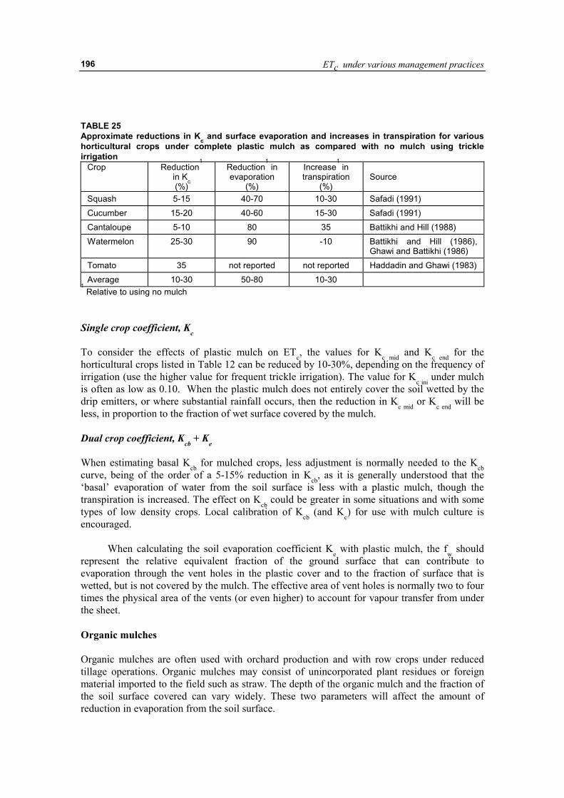
ETc under various management practices
196
TABLE 25 Approximate reductions in Kc and surface evaporation and increases in transpiration for various horticultural crops under complete plastic mulch as compared with no mulch using trickle irrigation
Crop Reduction1
in Kc (%)
Reduction1 in
evaporation (%)
Increase1 in
transpiration (%)
Source
Squash 5-15 40-70 10-30 Safadi (1991) Cucumber 15-20 40-60 15-30 Safadi (1991) Cantaloupe 5-10 80 35 Battikhi and Hill (1988) Watermelon 25-30 90 -10 Battikhi and Hill (1986),
Ghawi and Battikhi (1986) Tomato 35 not reported not reported Haddadin and Ghawi (1983) Average 10-30 50-80 10-30
1 Relative to using no mulch
Single crop coefficient, Kc To consider the effects of plastic mulch on ETc, the values for Kc mid and Kc end for the horticultural crops listed in Table 12 can be reduced by 10-30%, depending on the frequency of irrigation (use the higher value for frequent trickle irrigation). The value for Kc ini under mulch is often as low as 0.10. When the plastic mulch does not entirely cover the soil wetted by the drip emitters, or where substantial rainfall occurs, then the reduction in Kc mid or Kc end will be less, in proportion to the fraction of wet surface covered by the mulch. Dual crop coefficient, Kcb + Ke When estimating basal Kcb for mulched crops, less adjustment is normally needed to the Kcb curve, being of the order of a 5-15% reduction in Kcb, as it is generally understood that the ‘basal’ evaporation of water from the soil surface is less with a plastic mulch, though the transpiration is increased. The effect on Kcb could be greater in some situations and with some types of low density crops. Local calibration of Kcb (and Kc) for use with mulch culture is encouraged.
When calculating the soil evaporation coefficient Ke with plastic mulch, the fw should represent the relative equivalent fraction of the ground surface that can contribute to evaporation through the vent holes in the plastic cover and to the fraction of surface that is wetted, but is not covered by the mulch. The effective area of vent holes is normally two to four times the physical area of the vents (or even higher) to account for vapour transfer from under the sheet. Organic mulches Organic mulches are often used with orchard production and with row crops under reduced tillage operations. Organic mulches may consist of unincorporated plant residues or foreign material imported to the field such as straw. The depth of the organic mulch and the fraction of the soil surface covered can vary widely. These two parameters will affect the amount of reduction in evaporation from the soil surface.
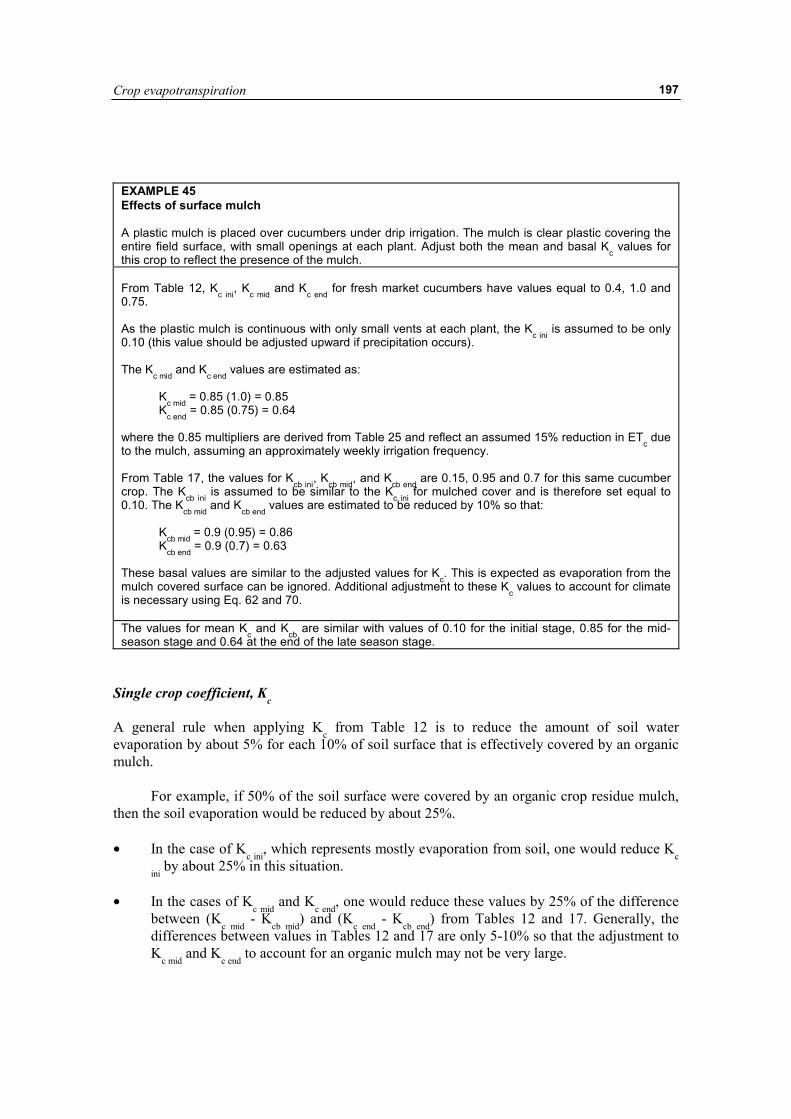
Crop evapotranspiration
197
EXAMPLE 45 Effects of surface mulch A plastic mulch is placed over cucumbers under drip irrigation. The mulch is clear plastic covering the entire field surface, with small openings at each plant. Adjust both the mean and basal Kc values for this crop to reflect the presence of the mulch. From Table 12, Kc ini, Kc mid and Kc end for fresh market cucumbers have values equal to 0.4, 1.0 and 0.75. As the plastic mulch is continuous with only small vents at each plant, the Kc ini is assumed to be only 0.10 (this value should be adjusted upward if precipitation occurs). The Kc mid and Kc end values are estimated as: Kc mid = 0.85 (1.0) = 0.85 Kc end = 0.85 (0.75) = 0.64 where the 0.85 multipliers are derived from Table 25 and reflect an assumed 15% reduction in ETc due to the mulch, assuming an approximately weekly irrigation frequency. From Table 17, the values for Kcb ini, Kcb mid, and Kcb end are 0.15, 0.95 and 0.7 for this same cucumber crop. The Kcb ini is assumed to be similar to the Kc ini for mulched cover and is therefore set equal to 0.10. The Kcb mid and Kcb end values are estimated to be reduced by 10% so that: Kcb mid = 0.9 (0.95) = 0.86 Kcb end = 0.9 (0.7) = 0.63 These basal values are similar to the adjusted values for Kc. This is expected as evaporation from the mulch covered surface can be ignored. Additional adjustment to these Kc values to account for climate is necessary using Eq. 62 and 70. The values for mean Kc and Kcb are similar with values of 0.10 for the initial stage, 0.85 for the mid-season stage and 0.64 at the end of the late season stage.
Single crop coefficient, Kc A general rule when applying Kc from Table 12 is to reduce the amount of soil water evaporation by about 5% for each 10% of soil surface that is effectively covered by an organic mulch.
For example, if 50% of the soil surface were covered by an organic crop residue mulch, then the soil evaporation would be reduced by about 25%. • In the case of Kc ini, which represents mostly evaporation from soil, one would reduce Kc
ini by about 25% in this situation. • In the cases of Kc mid and Kc end, one would reduce these values by 25% of the difference
between (Kc mid - Kcb mid) and (Kc end - Kcb end) from Tables 12 and 17. Generally, the differences between values in Tables 12 and 17 are only 5-10% so that the adjustment to Kc mid and Kc end to account for an organic mulch may not be very large.
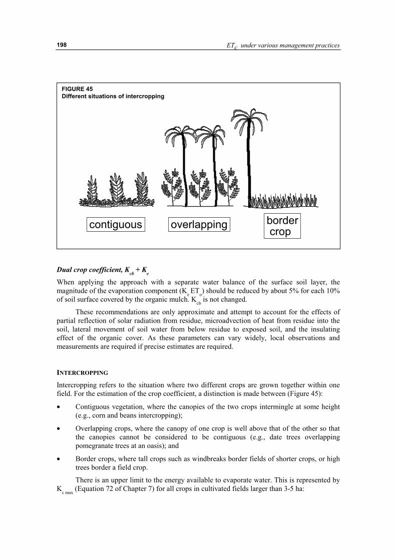
ETc under various management practices
198
Dual crop coefficient, Kcb + Ke
When applying the approach with a separate water balance of the surface soil layer, the magnitude of the evaporation component (Ke ETo) should be reduced by about 5% for each 10% of soil surface covered by the organic mulch. Kcb is not changed.
These recommendations are only approximate and attempt to account for the effects of partial reflection of solar radiation from residue, microadvection of heat from residue into the soil, lateral movement of soil water from below residue to exposed soil, and the insulating effect of the organic cover. As these parameters can vary widely, local observations and measurements are required if precise estimates are required. INTERCROPPING
Intercropping refers to the situation where two different crops are grown together within one field. For the estimation of the crop coefficient, a distinction is made between (Figure 45):
• Contiguous vegetation, where the canopies of the two crops intermingle at some height (e.g., corn and beans intercropping);
• Overlapping crops, where the canopy of one crop is well above that of the other so that the canopies cannot be considered to be contiguous (e.g., date trees overlapping pomegranate trees at an oasis); and
• Border crops, where tall crops such as windbreaks border fields of shorter crops, or high trees border a field crop.
There is an upper limit to the energy available to evaporate water. This is represented by Kc max (Equation 72 of Chapter 7) for all crops in cultivated fields larger than 3-5 ha:
FIGURE 45 Different situations of intercropping
contiguous overlapping border crop
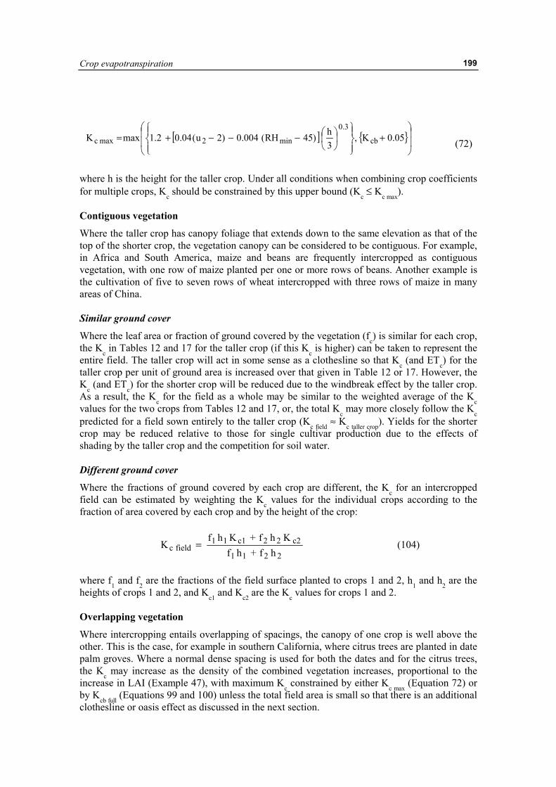
Crop evapotranspiration
199
[ ] { }��
�
�
��
�
�+
��
�
��
��
��
���
�−−−+= 05.0K,3h)45RH(004.0)2u(04.02.1maxK cb
3.0
min2maxc (72)
where h is the height for the taller crop. Under all conditions when combining crop coefficients for multiple crops, Kc should be constrained by this upper bound (Kc ≤ Kc max). Contiguous vegetation
Where the taller crop has canopy foliage that extends down to the same elevation as that of the top of the shorter crop, the vegetation canopy can be considered to be contiguous. For example, in Africa and South America, maize and beans are frequently intercropped as contiguous vegetation, with one row of maize planted per one or more rows of beans. Another example is the cultivation of five to seven rows of wheat intercropped with three rows of maize in many areas of China. Similar ground cover
Where the leaf area or fraction of ground covered by the vegetation (fc) is similar for each crop, the Kc in Tables 12 and 17 for the taller crop (if this Kc is higher) can be taken to represent the entire field. The taller crop will act in some sense as a clothesline so that Kc (and ETc) for the taller crop per unit of ground area is increased over that given in Table 12 or 17. However, the Kc (and ETc) for the shorter crop will be reduced due to the windbreak effect by the taller crop. As a result, the Kc for the field as a whole may be similar to the weighted average of the Kc values for the two crops from Tables 12 and 17, or, the total Kc may more closely follow the Kc predicted for a field sown entirely to the taller crop (Kc field ≈ Kc taller crop). Yields for the shorter crop may be reduced relative to those for single cultivar production due to the effects of shading by the taller crop and the competition for soil water. Different ground cover
Where the fractions of ground covered by each crop are different, the Kc for an intercropped field can be estimated by weighting the Kc values for the individual crops according to the fraction of area covered by each crop and by the height of the crop:
2211
c222c111fieldc hf+hf
Khf+KhfK = (104)
where f1 and f2 are the fractions of the field surface planted to crops 1 and 2, h1 and h2 are the heights of crops 1 and 2, and Kc1 and Kc2 are the Kc values for crops 1 and 2. Overlapping vegetation
Where intercropping entails overlapping of spacings, the canopy of one crop is well above the other. This is the case, for example in southern California, where citrus trees are planted in date palm groves. Where a normal dense spacing is used for both the dates and for the citrus trees, the Kc may increase as the density of the combined vegetation increases, proportional to the increase in LAI (Example 47), with maximum Kc constrained by either Kc max (Equation 72) or by Kcb full (Equations 99 and 100) unless the total field area is small so that there is an additional clothesline or oasis effect as discussed in the next section.
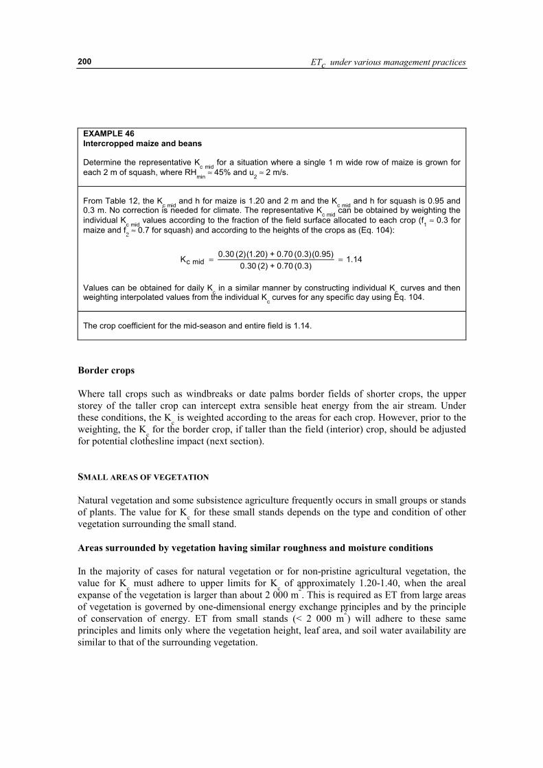
ETc under various management practices
200
EXAMPLE 46 Intercropped maize and beans Determine the representative Kc mid for a situation where a single 1 m wide row of maize is grown for each 2 m of squash, where RHmin ≈ 45% and u2 ≈ 2 m/s. From Table 12, the Kc mid and h for maize is 1.20 and 2 m and the Kc mid and h for squash is 0.95 and 0.3 m. No correction is needed for climate. The representative Kc mid can be obtained by weighting the individual Kc mid values according to the fraction of the field surface allocated to each crop (f1 ≈ 0.3 for maize and f2 ≈ 0.7 for squash) and according to the heights of the crops as (Eq. 104):
14.1)3.0(70.0+)2(30.0
)95.(0)3.0(70.0+)20.1()2(30.0K midc ==
Values can be obtained for daily Kc in a similar manner by constructing individual Kc curves and then weighting interpolated values from the individual Kc curves for any specific day using Eq. 104. The crop coefficient for the mid-season and entire field is 1.14.
Border crops Where tall crops such as windbreaks or date palms border fields of shorter crops, the upper storey of the taller crop can intercept extra sensible heat energy from the air stream. Under these conditions, the Kc is weighted according to the areas for each crop. However, prior to the weighting, the Kc for the border crop, if taller than the field (interior) crop, should be adjusted for potential clothesline impact (next section). SMALL AREAS OF VEGETATION Natural vegetation and some subsistence agriculture frequently occurs in small groups or stands of plants. The value for Kc for these small stands depends on the type and condition of other vegetation surrounding the small stand. Areas surrounded by vegetation having similar roughness and moisture conditions In the majority of cases for natural vegetation or for non-pristine agricultural vegetation, the value for Kc must adhere to upper limits for Kc of approximately 1.20-1.40, when the areal expanse of the vegetation is larger than about 2 000 m
2. This is required as ET from large areas
of vegetation is governed by one-dimensional energy exchange principles and by the principle of conservation of energy. ET from small stands (< 2 000 m
2) will adhere to these same
principles and limits only where the vegetation height, leaf area, and soil water availability are similar to that of the surrounding vegetation.
Crop evapotranspiration
201
EXAMPLE 47 Overlapping vegetation A 20 ha date palm grove in Palm Desert, California, the United States has a tree spacing of 6 m. Interplanted among the rows of palms are small orange trees (50% canopy) on a 6 m spacing. The palm and citrus trees are 3 m from one another in the rows. Height of the palms is 10 m and height of the citrus is 3 m. The canopy foliage of the palms is well above that of the citrus so that the canopies cannot be considered contiguous. Mean average RHmin during the mid-season is 20% and u2 = 2 m/s. The Kc mid from Table 12 for dates is 0.95 and when adjusted for humidity and wind using Eq. 62 is Kc mid = 1.09. The Kc mid from Table 12 for citrus having 50% canopy with no ground cover is 0.60 and when adjusted for humidity and wind using Eq. 62 is Kc mid = 0.70. The interplanting of citrus among the date palms has increased the total leaf area of the orchard so that ETc for the combined planting (palms and citrus together) will be greater than for either planting alone. The estimated combined Kc mid will be estimated as a function of the increase in total LAI. First the LAI values of the individual plantings are estimated by inverting Eq. 97 to solve for LAI:
���
�
���
�
−
−−−=
mincfullcb
minccbKK
KK1ln4.1LAI
where Kc min is the minimum basal Kc for bare soil (≈ 0.15 to 0.20) and Kcb full is the maximum mid-season Kc expected for the crop if there were complete ground cover, calculated using Eq. 99. Based on Eq. 99, with h = 10 m for the date palms and h = 3 m for the citrus, the Kcb full values for the two crops, assuming complete ground cover for each, are Kcb full = 1.34 for palms and Kcb full = 1.30 for citrus (using RHmin = 20% and u2 = 2 m/s). These estimates ignore effects of any unique stomatal control. Therefore, using the above equation, the effective LAI values of the date palms and citrus are estimated to be approximately:
LAIpalms = - 1.4 ln[1-(1.09-0.15)/(1.34-0.15)] = 2.2 LAIcitrus = - 1.4 ln[1-(0.70-0.15)/(1.30-0.15)] = 0.9
Therefore, the effective LAI for the date palm-citrus combination is estimated to be approximately LAIcombined = LAIpalms + LAIcitrus = 2.2 + 0.9 = 3.1. The increase in Kc mid for the date palm orchard resulting from the increase in LAI from the interplanting of citrus is estimated using a ratio of the LAI-based function introduced in Eq. 97. This results in the relationship:
( )( )���
�
���
�
−−−−
=cropsingle
combinedcropsingle,midcmid c LAI0.7exp1
LAI0.7exp1KK
where LAIcombined is the LAI for the two intercropped plantings combined and LAIsingle crop is the LAI for the taller, single crop. Kc mid single crop is the mid-season Kc for the taller, single crop (in this case the date palms). In this application, the above equation is solved as:
( )( ) 23.1
)2.2(0.7exp1)1.3(0.7exp109.1K mid c =��
���
�
−−−−=
Therefore, the Kc mid estimated for the complex of date palms and citrus together is 1.23. This value is compared with the maximum expected Kc based on energy limitations, represented by Kc max of Eq. 72 which in this case for h=10 m is Kc max = 1.34. Because Kc mid < Kc max (i.e., 1.23 < 1.34), the Kc mid = 1.23 is accepted as the approximate estimate of the Kc mid for the intercropped field.
ETc under various management practices
202
Clothesline and oasis effects
Under the clothesline effect, where vegetation height is greater than that of the surroundings (different roughness conditions), or under the oasis effect, where vegetation has higher soil water availability than the surroundings (different moisture conditions), the peak Kc values may exceed the 1.20-1.40 limit. The user should exercise caution when extrapolating ET measurements taken from these sorts of vegetation stands or plots to larger stands or regions as an overestimation of regional ET may occur.
Small expanses of tall vegetation that are surrounded by shorter cover can exhibit a clothesline effect. This occurs where turbulent transport of sensible heat into the canopy and transport of vapour away from the canopy is increased by the ‘broadsiding’ of wind horizontally into the taller vegetation. In addition, the internal boundary layer above the vegetation may not be in equilibrium with the new surface. Therefore, ET from the isolated expanses, on a per unit area basis, may be significantly greater than the corresponding ETo computed for the grass reference. Examples of the clothesline or oasis effects would be ET from a single row of trees surrounded by short vegetation or surrounded by a dry non-cropped field, or ET from a narrow strip of cattails (a hydrophytic vegetation) along a stream channel. Kc values up to and exceeding two have been recorded for such situations.
Where ET estimates are needed for such small, isolated expanses of vegetation surrounded by shorter cover (clothesline effect) or dry land (oasis effect), then the Kc may exceed the grass reference by 100% or more. Estimates of Kc for the expanses of vegetation should contain u2, RHmin and h parameters to adjust Kc values, and parameters expressing the aridity of the surrounding area, the general width of the vegetation stand and the ability of the wind to penetrate into the vegetation. The equation should also consider the LAI of the vegetation to account for the ability of the vegetation to conduct and transpire the amount of water demanded by the clothesline/climatic condition. An upper limit of 2.5 is usually placed on Kc to represent an upper limit on the stomatal capacity of the vegetation to supply water vapour to the air stream under the clothesline or oasis conditions. For vegetation with a great leaf resistance, such as for some types of desert vegetation or trees, the upper limit should be multiplied by a resistance correction factor, Fr, calculated in Chapter 9 using Equation 102.
Figure 46 presents example curves of Kc for small areas of vegetation versus vegetation stand width, for conditions where u2 = 2 m/s, RHmin = 30%, vegetation height = 2 m, and LAI = 3. The upper curve represents conditions where the specific vegetation is surrounded by dead vegetation, dry bare soil, or even gravel or asphalt. In this situation, large amounts of sensible heat are generated from the surrounding area due to the lack of ET. Some of this sensible heat is advected into the vegetation downwind. The lower curve represents conditions where the vegetation is surrounded by well-watered grass. In this situation, there is much less sensible heat available from the surrounding area to increase ET (and Kc) of vegetation downwind. The influence of the aridity of the surroundings on the Kc for a small expanse is apparent. The two curves shown will change with changes in u2, RHmin, h, and LAI. The user is cautioned that Figure 46 provides only general estimates of Kc under clothesline and oasis conditions. These estimates should be verified where possible using valid local measurements.
ET estimates from large expanses of vegetation or from small expanses of vegetation that are surrounded by mixtures of other vegetation having similar roughness and moisture conditions should almost always be less than or equal to 1.4 ETo, even under arid conditions.
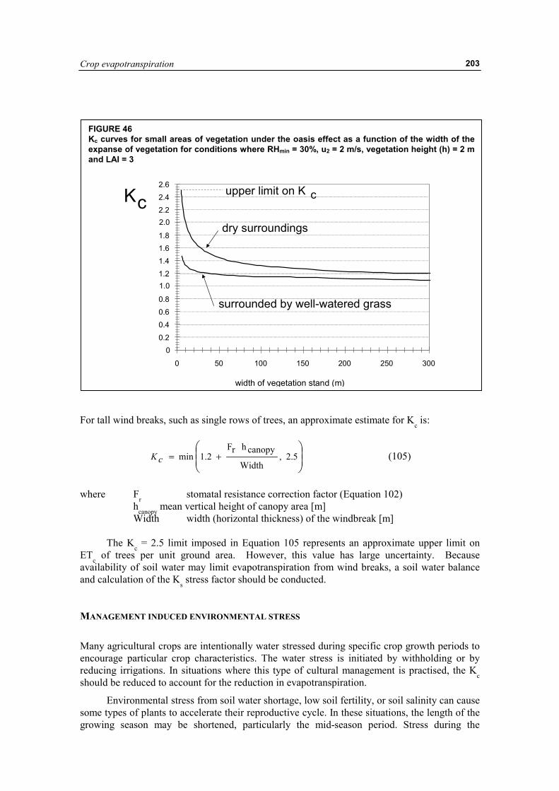
Crop evapotranspiration
203
For tall wind breaks, such as single rows of trees, an approximate estimate for Kc is:
��
�
�
��
�
�+= 5.2,
Width
canopyhrF2.1mincK (105)
where Fr stomatal resistance correction factor (Equation 102) hcanopy mean vertical height of canopy area [m] Width width (horizontal thickness) of the windbreak [m]
The Kc = 2.5 limit imposed in Equation 105 represents an approximate upper limit on ETc of trees per unit ground area. However, this value has large uncertainty. Because availability of soil water may limit evapotranspiration from wind breaks, a soil water balance and calculation of the Ks stress factor should be conducted. MANAGEMENT INDUCED ENVIRONMENTAL STRESS
Many agricultural crops are intentionally water stressed during specific crop growth periods to encourage particular crop characteristics. The water stress is initiated by withholding or by reducing irrigations. In situations where this type of cultural management is practised, the Kc should be reduced to account for the reduction in evapotranspiration.
Environmental stress from soil water shortage, low soil fertility, or soil salinity can cause some types of plants to accelerate their reproductive cycle. In these situations, the length of the growing season may be shortened, particularly the mid-season period. Stress during the
FIGURE 46 Kc curves for small areas of vegetation under the oasis effect as a function of the width of the expanse of vegetation for conditions where RHmin = 30%, u2 = 2 m/s, vegetation height (h) = 2 m and LAI = 3
K c dry surroundings
surrounded by well-watered grass
upper limit on K c
00.20.40.60.8
1.01.21.41.61.8
2.02.22.42.6
0 50 100 150 200 250 300
width of vegetation stand (m)
ETc under various management practices
204
development period may increase the length of that period. Therefore, the length of the mid-season, Lmid, and perhaps the lengths of the development and late seasons may need to be adjusted for environmentally stressed or damaged vegetation. Local research and observation is critical to identify the magnitudes and extent of these adjustments. Some examples of modifications to Kc and to lengths of growing periods are described below. Alfalfa seed
Some forage crops such as alfalfa that are grown for seed production are intentionally water stressed to reduce the amount of vegetation and to encourage increased production of flowers and seed. In areas subject to freezing winters, the reduction in Kc for deep rooted crops such as alfalfa depends upon the amount of water made available from precipitation during the dormant (winter) season and upon the amount of rainfall and limited irrigation during the growing season. Therefore, the effects of the intentional stress on the values for Kc should be modelled using the basal crop procedure presented in Chapter 7 and the Ks coefficient and water balance procedure presented in Chapter 8. Cotton
In cotton production, soil water stress may be initiated during the development period to delay flower development and to encourage boll development. This practice retards the growth rate of the cotton plant and delays the date of full cover. For cotton, the attainment of full cover and the beginning of the mid-season generally occurs when the LAI reaches approximately three. When soil water stress and growth retardation is practised, full cover may occur after the beginning of flowering. The effect of stress during the development period on ETc can be incorporated into the Kc curve by extending the length of the development period into the mid-season period. The length of the total season generally remains the same. Sugar beets
Sugar beets are frequently managed to initiate mild soil water stress during the late season period to dehydrate roots and concentrate sugars. A terminal irrigation may be needed just prior to harvest to assist in root extraction. When this type of water stress is practised, the value for Kc end is reduced from 1.0 to 0.6 (Table 12, Footnote 5). Coffee
Coffee plants are often intentionally water stressed to reduce vegetation growth and to encourage development of berries. Under these conditions, Kc values from Table 12 should be reduced. In addition, coffee fields may be bordered by trees that serve as windbreaks. The effect of windbreaks is to reduce the Kc of the coffee plants due to a reduction in wind and solar radiation over the plants. The reduction in Kc could be significant where windbreaks are tall and frequent. However, the Kc for the entire field area, including the windbreaks, may be increased by the presence of the trees, relative to the values for Kc for coffee shown in Table 12, due to increased total leaf area of the coffee-tree combination and the increased aerodynamic roughness. Tea
Initiation and development of new leaves on tea plants often occurs following the start of the rainy season. During the dry season, initiation of new leaves is slow or non-existent. The transpiration from older leaves is lower than for new leaves due to effects of leaf age on

Crop evapotranspiration
205
stomatal conductance. Therefore, the Kc, when leaves have aged (more than 2-3 months old), will be perhaps 10-20% lower than shown in Tables 12 and 17. Similar to coffee, tea fields may be bordered by trees that serve as windbreaks. The effect of windbreaks is to reduce the Kc of the tea plants, but to potentially increase the Kc for the entire plantation, as described for coffee. Olives
Growers may increase spacings of olive trees under rainfed conditions in areas with less rainfall. This is done to increase the ground area per tree that contributes infiltrated rain to transpiration of the tree. For example, in Tunisia, the spacing of olive trees changes from the north to the south, in proportion to annual rainfall. The tree spacing influences the Kc for the crop (Example 43).

ETc under various management practices
206
Crop evapotranspiration
207
Chapter 11
ETc during non-growing periods
This chapter describes procedures for predicting ETc during non-growing periods. Non-growing periods are defined as periods during which no agricultural crop has been planted. In temperate climates, non-growing periods may include periods of frost and continuously frozen conditions. TYPES OF SURFACE CONDITIONS
The type and condition of the ground surface during non-growing periods dictates the range for ETc. Where the surface is bare soil, then the Kc will be quite similar to the Kc ini predicted in Chapter 6. Where the surface is covered by nearly dead vegetation or some type of organic mulch or crop residue, then the Kc will be similar to that for agriculture that uses a surface mulch. Where the surface is covered by weed growth or growth of ‘volunteer’ plants, then the Kc will vary according to the leaf area or fraction of ground covered by the vegetation and by the availability of soil water. Where the surface is snow covered or frozen, then the Kc is difficult to predict and a constant value for ETc may have to be assumed. Bare soil
Single crop coefficient
Where the ground is left mostly bare following harvest, then the Kc following harvest will be strongly influenced by the frequency and amount of precipitation. Kc for bare soil can be calculated as Kc = Kc ini where Kc ini is calculated using the procedure of Chapter 6. Dual crop coefficient
Where a daily soil water balance can be applied, the user may elect to apply the dual Kc approach of Chapter 7. In this situation, the topsoil layer may dry to very low water contents during periods having no precipitation. Therefore, the values for Kcb and for Kc min in Equations 71 and 76 should be set equal to zero. This provides for the opportunity to predict ETc = 0 during long periods having no rainfall. This is necessary to preserve the water balance of the evaporation layer and of the root zone in total. The daily water balance calculation, given Kcb = 0, will provide the most accurate estimates of ETc during the non-growing periods. Surface covered with dead vegetation
Single crop coefficient
Where the ground surface has a plant residue or other dead organic mulch cover, or where part of the unharvested crop remains suspended above the surface in a dead or senesced condition, then the surface will respond similarly to a surface covered by mulch. In this case, Kc can be
ETc during non-growing periods
208
set equal to Kc ini as predicted from figures 29 and 30, but the value for Kc ini can be reduced by about 5% for each 10% of soil surface that is effectively covered by an organic mulch. Dual crop coefficient
Evaporation from dead, wet vegetation can be substantial for a few days following a precipitation event. Therefore, in the dual Kc approach, the value for fc should be set equal to zero to reflect the lack of green cover and fw should be set equal to 1.0 to reflect the wetting of both soil and mulch cover by precipitation.
The dead mulch or vegetation will dry more quickly than would the underlying soil if it were exposed. In addition, the soil will be protected somewhat from evaporation by the dead mulch or vegetation cover. Therefore, total evaporation losses will be less than the TEW predicted from Equation 73. This can be accounted for by reducing the value for TEW by 5% for each 10% of soil surface that is effectively covered by an organic mulch. The value for REW should be limited to less than or equal to that for TEW. Surface covered with live vegetation During frost-free periods following harvest, weeds may begin to germinate and grow. This vegetation is supplied with water from storage in the soil profile and from any rainfall. In addition, crop seed lost during harvest may germinate following rainfall events and add to the ground cover. The amount of ground surface covered by vegetation will depend on the severity of weed infestation; the density of the volunteer crop; the frequency and extent of soil tillage; the availability of soil water or rain, and any damage by frost.
The value for Kcb during the non-growing period can be predicted over time according to the amount of vegetation covering the surface. This can be done through estimates of LAI using Equation 97 or estimates of the fraction of ground cover, fc, using Equation 98. Single crop coefficient In the single crop coefficient approach, the value for Kcb determined using procedures in Chapter 9 can be converted into an equivalent Kc by adding 0.05 to 0.15 according to the frequency of rainfall and surface wetting.
It is important that the Kc for vegetation during the non-growing period be limited according to the amount of soil water available to supply evapotranspiration. Otherwise, the law of conservation of mass will be violated. Under all conditions, the integration of Kc ETo over the course of the non-growing period cannot exceed the sum of the precipitation occurring during the period plus any residual soil water in the root zone following harvest that can be depleted by the subsequent vegetation. The root zone in this case is the root zone for the weed or volunteer crops. A daily soil water balance may provide for the best estimate of soil water induced stress and associated reduction in Kc and ETc. Dual crop coefficient Under the dual crop coefficient approach, Kcb can be predicted according to the amount of surface that is covered by vegetation using Equation 97 or 98. Then, a full daily soil water
Crop evapotranspiration
209
balance of the topsoil together with a full daily soil water balance of the root zone can be employed as described in Chapter 7. The soil water balances will automatically adhere to the law of conservation of mass, so that total ETc from the weed or volunteer vegetation will not be overestimated. Again, because the topsoil layer may dry to below wilting point under conditions of sparse rainfall, the values for Kcb and Kc min used in Equations 71 and 76 should be set equal to zero. In this manner, the daily soil water balance with dual Kc calculations can progress throughout the non-growing period with good results. Frozen or snow covered surfaces Where the ground surface is snow covered or frozen, any vegetation will be largely non-responsive and non-contributing to ETc, and the amount of ETc will be closely related to the availability of free water at the surface and to the albedo of the surface.
The albedo of snow covered surfaces can range from 0.40 for old, dirty snow cover to 0.90 for fresh, dry snow. Therefore, the ETc for snow cover will be less than ETo for grass, as 25-85% less shortwave energy is available. In addition, some energy must be used to melt the snow before evaporation.
The use of ETo under such conditions is of limited value, as the assumption of conditions sustaining a green grass cover is violated. It is even possible to obtain negative values for ETo on some winter days where the longwave radiation from the surface is large and the vapour pressure deficit is small. It is under these conditions that net condensation of water from the atmosphere is possible. This would be similar to negative evaporation.
Given the limited value of ETo (or even ETp) under snow covered or frozen conditions, a single, average value may be best used to predict ETc. Wright (1993) found that ETc averaged 1 mm/day over winter periods at Kimberly, Idaho, the United States, that were six months long (1 October to 30 March). The latitude of Kimberly is 42°N and the elevation is about 1 200 m. Over the six-year study period, the ground was 50% covered by snow for 25% of the time from 1 October to 30 March. The ground, when exposed, was frozen about 50% of the time. The Kc averaged 0.25 during periods when the soil was not frozen but where frosts were occurring (October and early November). When the ground had 50% snow cover or greater, the ETc averaged only 0.4 mm/day. Wright found that over the six-month non-growing period, total cumulative ETc exceeded precipitation by about 50 mm.
Figure 47 shows the mean measurements of ETc during the 1985-1991 study period. The measurements have high correspondence to the total shortwave radiation energy available on a clear day, Rso, estimated as 0.75 Ra. There is some lag between ETc and Rso and Rs caused by cooler temperatures in January – March as compared to the October – December period. The ETc/Rso ratio averaged only 0.17 over the six-month period, and averaged 0.11 from 1 Dec. – 10 Mar. The ETc/Rs ratio averaged 0.23 over the six-month period, and averaged 0.15 from 1 Dec. – 10 Mar.
A similar study conducted in Logan, Utah, the United States (latitude 41.6°N, elevation 1 350 m) over an eight-year period showed that ETc varied widely with soil surface wetness and air temperature during the winter months. The ‘average’ Kc from November to March was 0.5 for days having no snow cover. For days with snow cover, ‘ETc’ ranged from 0 to 1.5 mm/day. Similarly, Kc is about 0.4 for winter wheat during frozen periods in the region of northern China (latitude near 39°N.

ETc during non-growing periods
210
Single Crop Coefficient The above procedure can provide estimates for the single Kc during non-growing season periods having snow cover or freezing conditions. However, the actual value for Kc is known to vary widely and will be less when water is less available at the soil surface. Dual Crop Coefficient A daily soil water balance using the dual crop coefficient approach is necessary to accurately predict ETc under freezing and snow cover conditions. In the dual crop coefficient method, a daily water balance is conducted for the topsoil and the estimate for Kc can be reduced according to available water. However, in addition to the limited validity of the concept of ETo under frozen or snow covered conditions, the evaporation coefficient, Ke, may be reduced when the ground surface is frozen, as the water in a frozen state is less available.
Other, more complex models for predicting ETc under non-growing season conditions, snow cover, and freezing, are available in the literature and should be consulted and perhaps applied when precise estimates for ETc are needed. Some of these are listed in section K of the References.
FIGURE 47 Mean evapotranspiration measured during non-growing, winter periods at Kimberly, Idaho, United States by Wright (1993)
0.0
0.5
1.0
1.5
2.0
2.5
3.0
3.5
0
2
4
6
8
10
ET ,
mm
/day
and
ratio
s
Sola
r rad
iatio
n (R
),
mm
/day
c
so
ETcET /Rc so
Rso
280 300 320 340 360 20 40 60 80day of the year
Rs
ET /Rc s
Crop evapotranspiration
211
Annex 1
Units and symbols
PREFIXES Units can be used as such or in multiples: Tera (T) and which is 1012 Centi (c) 10-2 Giga (G) 109 Milli (m) 10-3 Mega (M) 106 Micro (µ) 10-6 Kilo (k) 103 Nano (n) 10-9 Hecto (h) 102 Pico (p) 10-12 Deca (da) 101 Femto (f) 10-15 Deci (d) 10-1 Atto (a) 10-18 TEMPERATURE Standard unit: degree Celsius (°C) _________________________________________________________ degree Fahrenheit (°F) (°C) = (°F-32) 5/9 Kelvin (K) 1 K = (°C) + 273.16 PRESSURE (air pressure, vapour pressure) Standard unit: kilopascal (kPa) _______________________________________________________________ millibar (mbar) 1 mbar = 0.1 kPa bar 1 bar = 100 kPa centimetre of water (cm) 1 cm of water = 0.09807 kPa millimetre of mercury (mmHg) 1 mmHg = 0.1333 kPa atmospheres (atm) 1 atm = 101.325 kPa pound per square inch (psi) 1 psi = 6.896 kPa
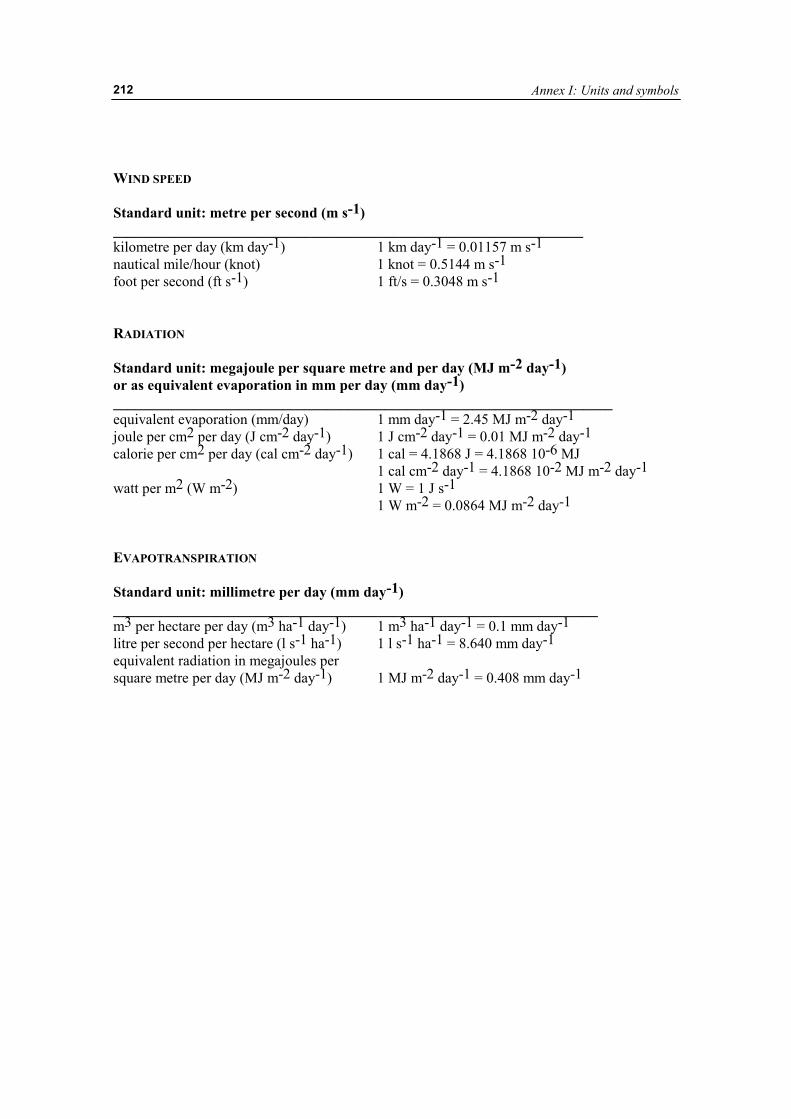
Annex I: Units and symbols
212
WIND SPEED Standard unit: metre per second (m s-1) ________________________________________________________________ kilometre per day (km day-1) 1 km day-1 = 0.01157 m s-1 nautical mile/hour (knot) 1 knot = 0.5144 m s-1 foot per second (ft s-1) 1 ft/s = 0.3048 m s-1 RADIATION Standard unit: megajoule per square metre and per day (MJ m-2 day-1) or as equivalent evaporation in mm per day (mm day-1) ____________________________________________________________________ equivalent evaporation (mm/day) 1 mm day-1 = 2.45 MJ m-2 day-1 joule per cm2 per day (J cm-2 day-1) 1 J cm-2 day-1 = 0.01 MJ m-2 day-1 calorie per cm2 per day (cal cm-2 day-1) 1 cal = 4.1868 J = 4.1868 10-6 MJ 1 cal cm-2 day-1 = 4.1868 10-2 MJ m-2 day-1 watt per m2 (W m-2) 1 W = 1 J s-1 1 W m-2 = 0.0864 MJ m-2 day-1 EVAPOTRANSPIRATION Standard unit: millimetre per day (mm day-1) __________________________________________________________________ m3 per hectare per day (m3 ha-1 day-1) 1 m3 ha-1 day-1 = 0.1 mm day-1 litre per second per hectare (l s-1 ha-1) 1 l s-1 ha-1 = 8.640 mm day-1 equivalent radiation in megajoules per square metre per day (MJ m-2 day-1) 1 MJ m-2 day-1 = 0.408 mm day-1
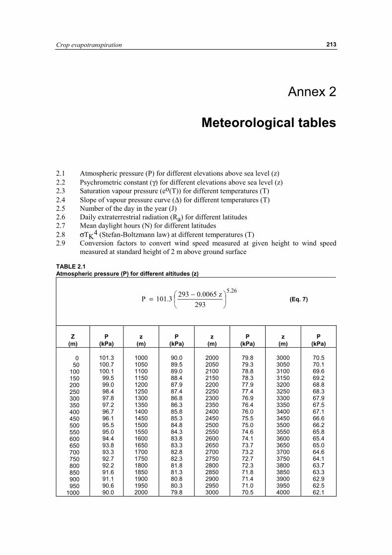
Crop evapotranspiration
213
Annex 2
Meteorological tables
2.1 Atmospheric pressure (P) for different elevations above sea level (z) 2.2 Psychrometric constant (γ) for different elevations above sea level (z) 2.3 Saturation vapour pressure (eo(T)) for different temperatures (T) 2.4 Slope of vapour pressure curve (∆) for different temperatures (T) 2.5 Number of the day in the year (J) 2.6 Daily extraterrestrial radiation (Ra) for different latitudes 2.7 Mean daylight hours (N) for different latitudes 2.8 σTK4 (Stefan-Boltzmann law) at different temperatures (T) 2.9 Conversion factors to convert wind speed measured at given height to wind speed
measured at standard height of 2 m above ground surface TABLE 2.1 Atmospheric pressure (P) for different altitudes (z)
��
���
� −=293
z0065.02933.101P26.5
(Eq. 7)
Z
(m)
P
(kPa)
z
(m)
P
(kPa)
z
(m)
P
(kPa)
z
(m)
P
(kPa)
0 50 100 150 200 250 300 350 400 450 500 550 600 650 700 750 800 850 900 950 1000
101.3 100.7 100.1 99.5 99.0 98.4 97.8 97.2 96.7 96.1 95.5 95.0 94.4 93.8 93.3 92.7 92.2 91.6 91.1 90.6 90.0
1000 1050 1100 1150 1200 1250 1300 1350 1400 1450 1500 1550 1600 1650 1700 1750 1800 1850 1900 1950 2000
90.0 89.5 89.0 88.4 87.9 87.4 86.8 86.3 85.8 85.3 84.8 84.3 83.8 83.3 82.8 82.3 81.8 81.3 80.8 80.3 79.8
2000 2050 2100 2150 2200 2250 2300 2350 2400 2450 2500 2550 2600 2650 2700 2750 2800 2850 2900 2950 3000
79.8 79.3 78.8 78.3 77.9 77.4 76.9 76.4 76.0 75.5 75.0 74.6 74.1 73.7 73.2 72.7 72.3 71.8 71.4 71.0 70.5
3000 3050 3100 3150 3200 3250 3300 3350 3400 3450 3500 3550 3600 3650 3700 3750 3800 3850 3900 3950 4000
70.5 70.1 69.6 69.2 68.8 68.3 67.9 67.5 67.1 66.6 66.2 65.8 65.4 65.0 64.6 64.1 63.7 63.3 62.9 62.5 62.1
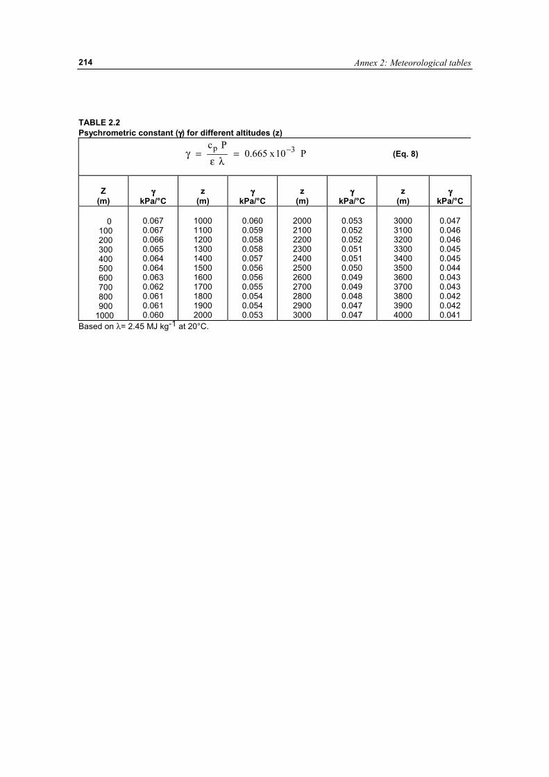
Annex 2: Meteorological tables
214
TABLE 2.2 Psychrometric constant (γγγγ) for different altitudes (z)
P10x665.0Pc 3p −=λε
=γ (Eq. 8)
Z
(m)
γγγγ
kPa/°C
z
(m)
γγγγ
kPa/°C
z
(m)
γγγγ
kPa/°C
z
(m)
γγγγ
kPa/°C
0 100 200 300 400 500 600 700 800 900 1000
0.067 0.067 0.066 0.065 0.064 0.064 0.063 0.062 0.061 0.061 0.060
1000 1100 1200 1300 1400 1500 1600 1700 1800 1900 2000
0.060 0.059 0.058 0.058 0.057 0.056 0.056 0.055 0.054 0.054 0.053
2000 2100 2200 2300 2400 2500 2600 2700 2800 2900 3000
0.053 0.052 0.052 0.051 0.051 0.050 0.049 0.049 0.048 0.047 0.047
3000 3100 3200 3300 3400 3500 3600 3700 3800 3900 4000
0.047 0.046 0.046 0.045 0.045 0.044 0.043 0.043 0.042 0.042 0.041
Based on λ= 2.45 MJ kg-1 at 20°C.
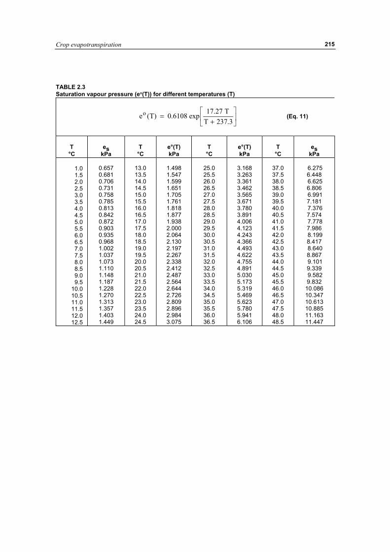
Crop evapotranspiration
215
TABLE 2.3 Saturation vapour pressure (eo(T)) for different temperatures (T)
��
���
�
+=
3.237TT27.17exp6108.0)T(eo (Eq. 11)
T °C
es
kPa
T °C
e°(T) kPa
T °C
e°(T) kPa
T °C
es
kPa
1.0 1.5
2.0 2.5
3.0 3.5
4.0 4.5
5.0 5.5
6.0 6.5
7.0 7.5
8.0 8.5
9.0 9.5
10.0 10.5 11.0 11.5 12.0 12.5
0.657 0.681 0.706 0.731 0.758 0.785 0.813 0.842 0.872 0.903 0.935 0.968 1.002 1.037 1.073 1.110 1.148 1.187 1.228 1.270 1.313 1.357 1.403 1.449
13.0 13.5 14.0 14.5 15.0 15.5 16.0 16.5 17.0 17.5 18.0 18.5 19.0 19.5 20.0 20.5 21.0 21.5 22.0 22.5 23.0 23.5 24.0 24.5
1.498 1.547 1.599 1.651 1.705 1.761 1.818 1.877 1.938 2.000 2.064 2.130 2.197 2.267 2.338 2.412 2.487 2.564 2.644 2.726 2.809 2.896 2.984 3.075
25.0 25.5 26.0 26.5 27.0 27.5 28.0 28.5 29.0 29.5 30.0 30.5 31.0 31.5 32.0 32.5 33.0 33.5 34.0 34.5 35.0 35.5 36.0 36.5
3.168 3.263 3.361 3.462 3.565 3.671 3.780 3.891 4.006 4.123 4.243 4.366 4.493 4.622 4.755 4.891 5.030 5.173 5.319 5.469 5.623 5.780 5.941 6.106
37.0 37.5 38.0 38.5 39.0 39.5 40.0 40.5 41.0 41.5 42.0 42.5 43.0 43.5 44.0 44.5 45.0 45.5 46.0 46.5 47.0 47.5 48.0 48.5
6.275 6.448 6.625 6.806 6.991 7.181 7.376 7.574 7.778 7.986 8.199 8.417 8.640 8.867 9.101 9.339 9.582 9.832
10.086 10.347 10.613 10.885 11.163 11.447
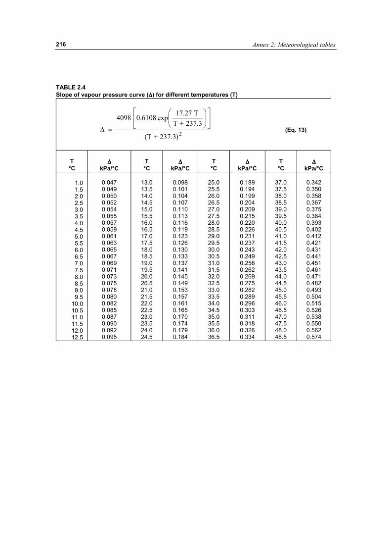
Annex 2: Meteorological tables
216
TABLE 2.4 Slope of vapour pressure curve (∆∆∆∆) for different temperatures (T)
2)37.32+(T
237.3+TT17.27exp0.61084098 �
�
���
����
�
�
=∆ (Eq. 13)
T °C
∆∆∆∆
kPa/°C
T °C
∆∆∆∆
kPa/°C
T °C
∆∆∆∆
kPa/°C
T °C
∆∆∆∆
kPa/°C
1.0 1.5
2.0 2.5
3.0 3.5
4.0 4.5
5.0 5.5
6.0 6.5
7.0 7.5
8.0 8.5
9.0 9.5
10.0 10.5 11.0 11.5 12.0 12.5
0.047 0.049 0.050 0.052 0.054 0.055 0.057 0.059 0.061 0.063 0.065 0.067 0.069 0.071 0.073 0.075 0.078 0.080 0.082 0.085 0.087 0.090 0.092 0.095
13.0 13.5 14.0 14.5 15.0 15.5 16.0 16.5 17.0 17.5 18.0 18.5 19.0 19.5 20.0 20.5 21.0 21.5 22.0 22.5 23.0 23.5 24.0 24.5
0.098 0.101 0.104 0.107 0.110 0.113 0.116 0.119 0.123 0.126 0.130 0.133 0.137 0.141 0.145 0.149 0.153 0.157 0.161 0.165 0.170 0.174 0.179 0.184
25.0 25.5 26.0 26.5 27.0 27.5 28.0 28.5 29.0 29.5 30.0 30.5 31.0 31.5 32.0 32.5 33.0 33.5 34.0 34.5 35.0 35.5 36.0 36.5
0.189 0.194 0.199 0.204 0.209 0.215 0.220 0.226 0.231 0.237 0.243 0.249 0.256 0.262 0.269 0.275 0.282 0.289 0.296 0.303 0.311 0.318 0.326 0.334
37.0 37.5 38.0 38.5 39.0 39.5 40.0 40.5 41.0 41.5 42.0 42.5 43.0 43.5 44.0 44.5 45.0 45.5 46.0 46.5 47.0 47.5 48.0 48.5
0.342 0.350 0.358 0.367 0.375 0.384 0.393 0.402 0.412 0.421 0.431 0.441 0.451 0.461 0.471 0.482 0.493 0.504 0.515 0.526 0.538 0.550 0.562 0.574
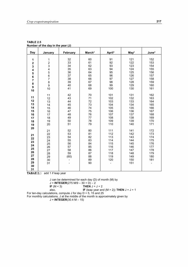
Crop evapotranspiration
217
TABLE 2.5 Number of the day in the year (J)
Day
January
February
March*
April*
May*
June*
1 2 3 4 5 6 7 8 9 10
11 12 13 14 15 16 17 18 19 20
21 22 23 24 25 26 27 28 29 30 31
1 2 3 4 5 6 7 8 9 10
11 12 13 14 15 16 17 18 19 20
21 22 23 24 25 26 27 28 29 30 31
32 33 34 35 36 37 38 39 40 41
42 43 44 45 46 47 48 49 50 51
52 53 54 55 56 57 58 59
(60) - -
60 61 62 63 64 65 66 67 68 69
70 71 72 73 74 75 76 77 78 79
80 81 82 83 84 85 86 87 88 89 90
91 92 93 94 95 96 97 98 99 100
101 102 103 104 105 106 107 108 109 110
111 112 113 114 115 116 117 118 119 120
-
121 122 123 124 125 126 127 128 129 130
131 132 133 134 135 136 137 138 139 140
141 142 143 144 145 146 147 148 149 150 151
152 153 154 155 156 157 158 159 160 161
162 163 164 165 166 167 168 169 170 171
172 173 174 175 176 177 178 179 180 181
-
ΤΑΒΛΕ 2.ΤΑΒΛΕ 2.ΤΑΒΛΕ 2.ΤΑΒΛΕ 2.���� add 1 if leap year
J can be determined for each day (D) of month (M) by J = INTEGER(275 M/9 – 30 + D) – 2 IF (M < 3) THEN J = J + 2 also, IF (leap year and (M > 2)) THEN J = J + 1
For ten-day calculations, compute J for day D = 5, 15 and 25 For monthly calculations, J at the middle of the month is approximately given by
J = INTEGER(30.4 M – 15)
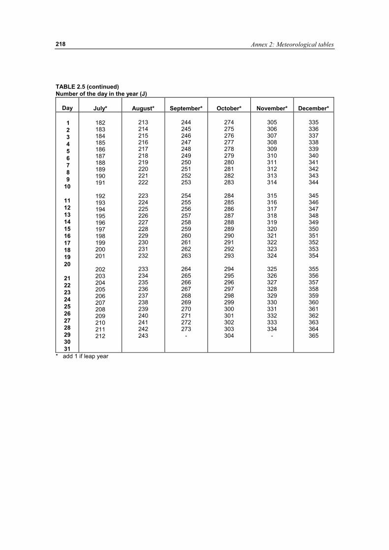
Annex 2: Meteorological tables
218
TABLE 2.5 (continued) Number of the day in the year (J)
Day
July*
August*
September*
October*
November*
December*
1 2 3 4 5 6 7 8 9 10
11 12 13 14 15 16 17 18 19 20
21 22 23 24 25 26 27 28 29 30 31
182 183 184 185 186 187 188 189 190 191
192 193 194 195 196 197 198 199 200 201
202 203 204 205 206 207 208 209 210 211 212
213 214 215 216 217 218 219 220 221 222
223 224 225 226 227 228 229 230 231 232
233 234 235 236 237 238 239 240 241 242 243
244 245 246 247 248 249 250 251 252 253
254 255 256 257 258 259 260 261 262 263
264 265 266 267 268 269 270 271 272 273
-
274 275 276 277 278 279 280 281 282 283
284 285 286 287 288 289 290 291 292 293
294 295 296 297 298 299 300 301 302 303 304
305 306 307 308 309 310 311 312 313 314
315 316 317 318 319 320 321 322 323 324
325 326 327 328 329 330 331 332 333 334
-
335 336 337 338 339 340 341 342 343 344
345 346 347 348 349 350 351 352 353 354
355 356 357 358 359 360 361 362 363 364 365
* add 1 if leap year

Crop evapotranspiration
219

Annex 2: Meteorological tables
220
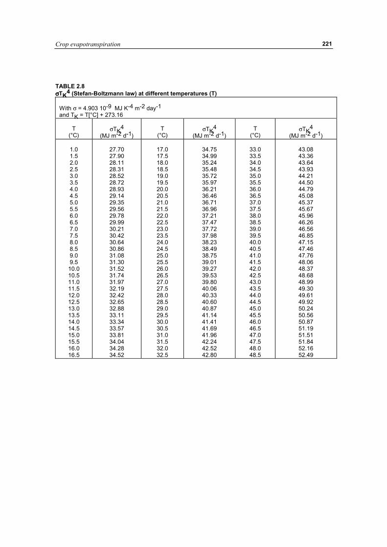
Crop evapotranspiration
221
TABLE 2.8 σσσσTK4 (Stefan-Boltzmann law) at different temperatures (T)
With σ = 4.903 10-9 MJ K-4 m-2 day-1 and TK = T[°C] + 273.16
T (°C)
σTK4
(MJ m-2 d-1)
T
(°C)
σTK4
(MJ m-2 d-1)
T
(°C)
σTK4
(MJ m-2 d-1)
1.0 1.5 2.0 2.5 3.0 3.5 4.0 4.5 5.0 5.5 6.0 6.5 7.0 7.5 8.0 8.5 9.0 9.5
10.0 10.5 11.0 11.5 12.0 12.5 13.0 13.5 14.0 14.5 15.0 15.5 16.0 16.5
27.70 27.90 28.11 28.31 28.52 28.72 28.93 29.14 29.35 29.56 29.78 29.99 30.21 30.42 30.64 30.86 31.08 31.30 31.52 31.74 31.97 32.19 32.42 32.65 32.88 33.11 33.34 33.57 33.81 34.04 34.28 34.52
17.0 17.5 18.0 18.5 19.0 19.5 20.0 20.5 21.0 21.5 22.0 22.5 23.0 23.5 24.0 24.5 25.0 25.5 26.0 26.5 27.0 27.5 28.0 28.5 29.0 29.5 30.0 30.5 31.0 31.5 32.0 32.5
34.75 34.99 35.24 35.48 35.72 35.97 36.21 36.46 36.71 36.96 37.21 37.47 37.72 37.98 38.23 38.49 38.75 39.01 39.27 39.53 39.80 40.06 40.33 40.60 40.87 41.14 41.41 41.69 41.96 42.24 42.52 42.80
33.0 33.5 34.0 34.5 35.0 35.5 36.0 36.5 37.0 37.5 38.0 38.5 39.0 39.5 40.0 40.5 41.0 41.5 42.0 42.5 43.0 43.5 44.0 44.5 45.0 45.5 46.0 46.5 47.0 47.5 48.0 48.5
43.08 43.36 43.64 43.93 44.21 44.50 44.79 45.08 45.37 45.67 45.96 46.26 46.56 46.85 47.15 47.46 47.76 48.06 48.37 48.68 48.99 49.30 49.61 49.92 50.24 50.56 50.87 51.19 51.51 51.84 52.16 52.49
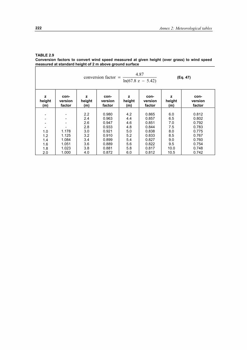
Annex 2: Meteorological tables
222
TABLE 2.9 Conversion factors to convert wind speed measured at given height (over grass) to wind speed measured at standard height of 2 m above ground surface
)42.5z8.67ln(
87.4factorconversion−
= (Eq. 47)
z height
(m)
con-
version factor
z
height (m)
con-
version factor
z
height (m)
con-
version factor
z
height (m)
con-
version factor
- - - -
1.0 1.2 1.4 1.6 1.8 2.0
- - - -
1.178 1.125 1.084 1.051 1.023 1.000
2.2 2.4 2.6 2.8 3.0 3.2 3.4 3.6 3.8 4.0
0.980 0.963 0.947 0.933 0.921 0.910 0.899 0.889 0.881 0.872
4.2 4.4 4.6 4.8 5.0 5.2 5.4 5.6 5.8 6.0
0.865 0.857 0.851 0.844 0.838 0.833 0.827 0.822 0.817 0.812
6.0 6.5 7.0 7.5 8.0 8.5 9.0 9.5
10.0 10.5
0.812 0.802 0.792 0.783 0.775 0.767 0.760 0.754 0.748 0.742
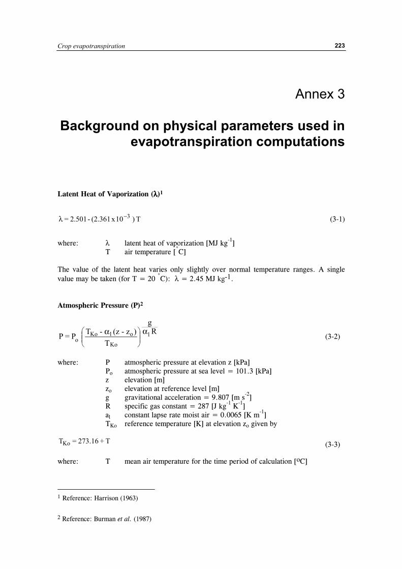
Crop evapotranspiration
223
Annex 3
Background on physical parameters used in evapotranspiration computations
Latent Heat of Vaporization (λλλλ)1
T ) 10 x(2.361 - 2.501 = 3−λ (3-1)
where: λ latent heat of vaporization [MJ kg-1] T air temperature [°C]
The value of the latent heat varies only slightly over normal temperature ranges. A single value may be taken (for T = 20 °C): λ = 2.45 MJ kg-1.
Atmospheric Pressure (P)2
���
����
� α αT
)z-(z- T Rg
P = PKo
o1Ko 1o (3-2)
where: P atmospheric pressure at elevation z [kPa]
Po atmospheric pressure at sea level = 101.3 [kPa] z elevation [m] zo elevation at reference level [m] g gravitational acceleration = 9.807 [m s-2] R specific gas constant = 287 [J kg-1 K-1] al constant lapse rate moist air = 0.0065 [K m-1] TKo reference temperature [K] at elevation zo given by
T + 273.16 = TKo (3-3)
where: T mean air temperature for the time period of calculation [oC]
1 Reference: Harrison (1963)
2 Reference: Burman et al. (1987)
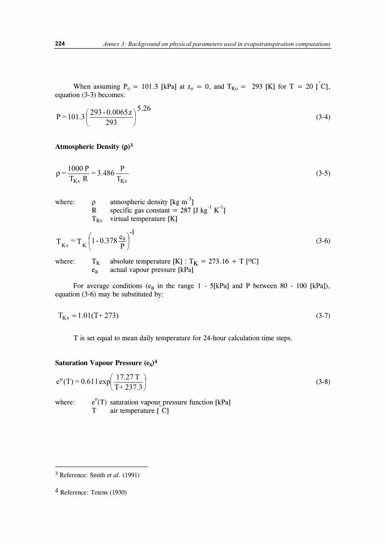
Annex 3: Background on physical parameters used in evapotranspiration computations
224
When assuming Po = 101.3 [kPa] at zo = 0, and TKo = 293 [K] for T = 20 [°C], equation (3-3) becomes:
��
���
�
293z0.0065-293 5.26
101.3 = P (3-4)
Atmospheric Density (ρρρρ)3
KvKv TP 3.486 =
R TP 1000 = ρ (3-5)
where: ρ atmospheric density [kg m-3] R specific gas constant = 287 [J kg-1 K-1] TKv virtual temperature [K]
��
���
�
Pe 0.378-1
1- T = T a
KKv (3-6)
where: TK absolute temperature [K] : TK = 273.16 + T [oC] ea actual vapour pressure [kPa]
For average conditions (ea in the range 1 - 5[kPa] and P between 80 - 100 [kPa]), equation (3-6) may be substituted by:
273)1.01(T+T Kv ≈ (3-7)
T is set equal to mean daily temperature for 24-hour calculation time steps.
Saturation Vapour Pressure (es)4
��
���
�
237.3T+T 17.27exp 0.611 = (T)eo (3-8)
where: eo(T) saturation vapour pressure function [kPa] T air temperature [°C]
3 Reference: Smith et al. (1991)
4 Reference: Tetens (1930)
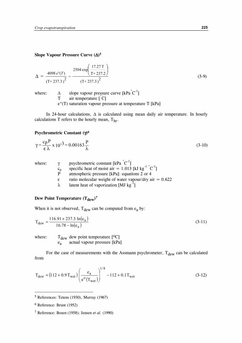
Crop evapotranspiration
225
Slope Vapour Pressure Curve (∆∆∆∆)5
)2237.3(T+
237.2T+
T17.27exp 2504
= )2237.3(T+
)(4098 =
��
���
�
∆° Te
(3-9)
where: ∆ slope vapour pressure curve [kPa°C-1] T air temperature [°C] e°(T) saturation vapour pressure at temperature T [kPa]
In 24-hour calculations, ∆ is calculated using mean daily air temperature. In hourly calculations T refers to the hourly mean, Thr.
Psychrometric Constant (γγγγ)6
λλεγ P 0.00163 = 10-3 x
Pcp = (3-10)
where: γ psychrometric constant [kPa °C-1] cp specific heat of moist air = 1.013 [kJ kg-1 °C-1] P atmospheric pressure [kPa]: equations 2 or 4 ε ratio molecular weight of water vapour/dry air = 0.622 λ latent heat of vaporization [MJ kg-1]
Dew Point Temperature (Tdew)7
When it is not observed, Tdew can be computed from ea by:
( )( )a
adew eln78.16
eln3.23791.116T
−+
= (3-11)
where: Tdew dew point temperature [oC] ea actual vapour pressure [kPa] For the case of measurements with the Assmann psychrometer, Tdew can be calculated from
( )( ) wet
8/1
weto
awetdew T1.0112
Te
eT9.0112T +−
��
�
�
��
�
�+= (3-12)
5 References: Tetens (1930), Murray (1967)
6 Reference: Brunt (1952)
7 Reference: Bosen (1958); Jensen et al. (1990)
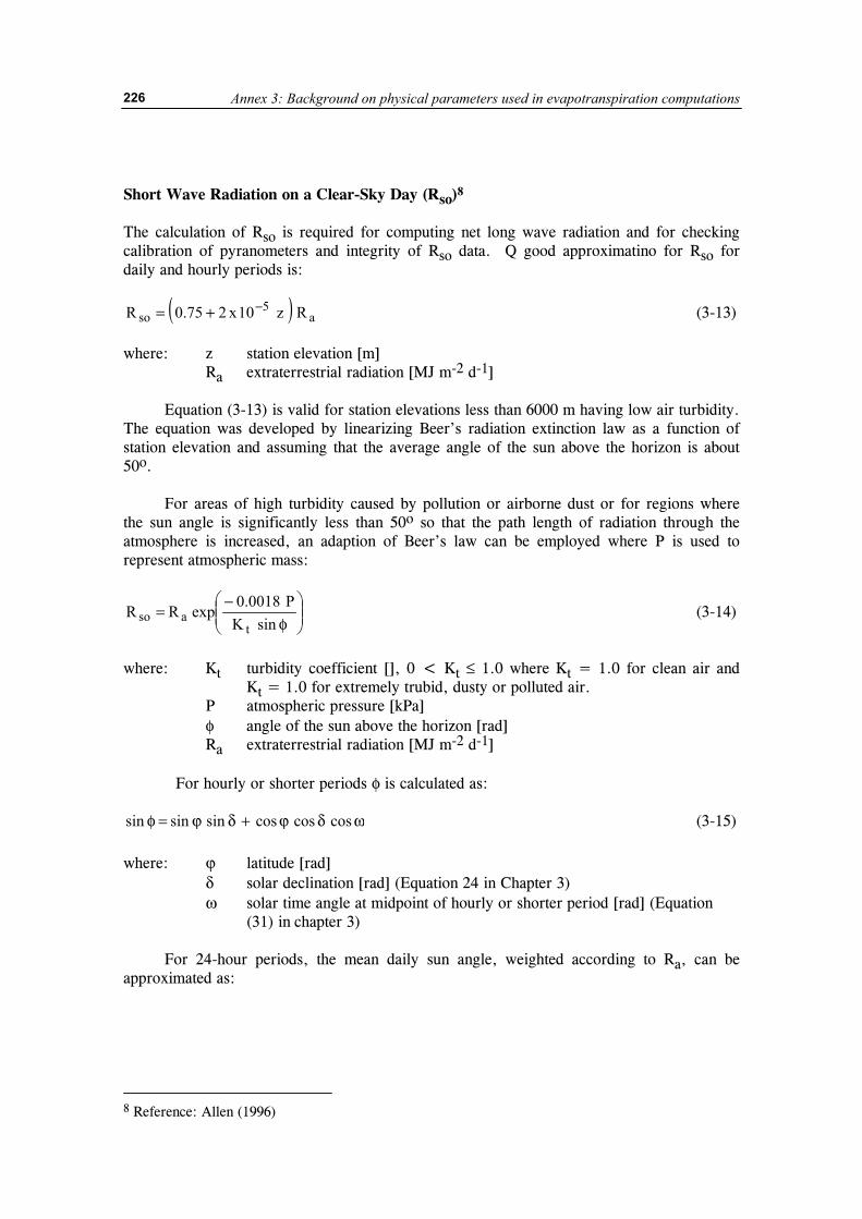
Annex 3: Background on physical parameters used in evapotranspiration computations
226
Short Wave Radiation on a Clear-Sky Day (Rso)8 The calculation of Rso is required for computing net long wave radiation and for checking calibration of pyranometers and integrity of Rso data. Q good approximatino for Rso for daily and hourly periods is:
( ) a5
so Rz10x275.0R −+= (3-13) where: z station elevation [m] Ra extraterrestrial radiation [MJ m-2 d-1] Equation (3-13) is valid for station elevations less than 6000 m having low air turbidity. The equation was developed by linearizing Beer’s radiation extinction law as a function of station elevation and assuming that the average angle of the sun above the horizon is about 50o. For areas of high turbidity caused by pollution or airborne dust or for regions where the sun angle is significantly less than 50o so that the path length of radiation through the atmosphere is increased, an adaption of Beer’s law can be employed where P is used to represent atmospheric mass:
���
����
�
φ−
=sinK
P0018.0expRRt
aso (3-14)
where: Kt turbidity coefficient [], 0 < Kt ≤ 1.0 where Kt = 1.0 for clean air and
Kt = 1.0 for extremely trubid, dusty or polluted air. P atmospheric pressure [kPa] φ angle of the sun above the horizon [rad] Ra extraterrestrial radiation [MJ m-2 d-1]
For hourly or shorter periods φ is calculated as:
ωδϕ+δϕ=φ coscoscossinsinsin (3-15) where: ϕ latitude [rad]
δ solar declination [rad] (Equation 24 in Chapter 3) ω solar time angle at midpoint of hourly or shorter period [rad] (Equation
(31) in chapter 3)
For 24-hour periods, the mean daily sun angle, weighted according to Ra, can be approximated as:
8 Reference: Allen (1996)
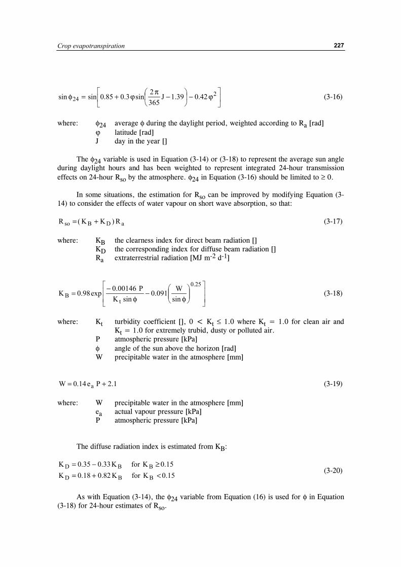
Crop evapotranspiration
227
��
���
�ϕ−�
�
�
� −π
ϕ+=φ 224 42.039.1J
3652sin3.085.0sinsin (3-16)
where: φ24 average φ during the daylight period, weighted according to Ra [rad]
ϕ latitude [rad] J day in the year []
The φ24 variable is used in Equation (3-14) or (3-18) to represent the average sun angle during daylight hours and has been weighted to represent integrated 24-hour transmission effects on 24-hour Rso by the atmosphere. φ24 in Equation (3-16) should be limited to ≥ 0. In some situations, the estimation for Rso can be improved by modifying Equation (3-14) to consider the effects of water vapour on short wave absorption, so that:
aDBso R)KK(R += (3-17) where: KB the clearness index for direct beam radiation []
KD the corresponding index for diffuse beam radiation [] Ra extraterrestrial radiation [MJ m-2 d-1]
��
�
�
��
�
�
���
�
�
φ−
φ−
=25.0
tB sin
W091.0sinK
P00146.0exp98.0K (3-18)
where: Kt turbidity coefficient [], 0 < Kt ≤ 1.0 where Kt = 1.0 for clean air and Kt = 1.0 for extremely trubid, dusty or polluted air.
P atmospheric pressure [kPa] φ angle of the sun above the horizon [rad] W precipitable water in the atmosphere [mm]
1.2Pe14.0W a += (3-19) where: W precipitable water in the atmosphere [mm] ea actual vapour pressure [kPa]
P atmospheric pressure [kPa]
The diffuse radiation index is estimated from KB:
15.0KforK82.018.0K15.0KforK33.035.0K
BBD
BBD<+=≥−=
(3-20)
As with Equation (3-14), the φ24 variable from Equation (16) is used for φ in Equation (3-18) for 24-hour estimates of Rso.

Annex 3: Background on physical parameters used in evapotranspiration computations
228
Ordinarily, Rso computed using Equations (3-13), (3-14) or (3-16) should plot as an upper envelope of measured Rs and is useful for checking calibration of instruments. This is illustrated in Annex 5.
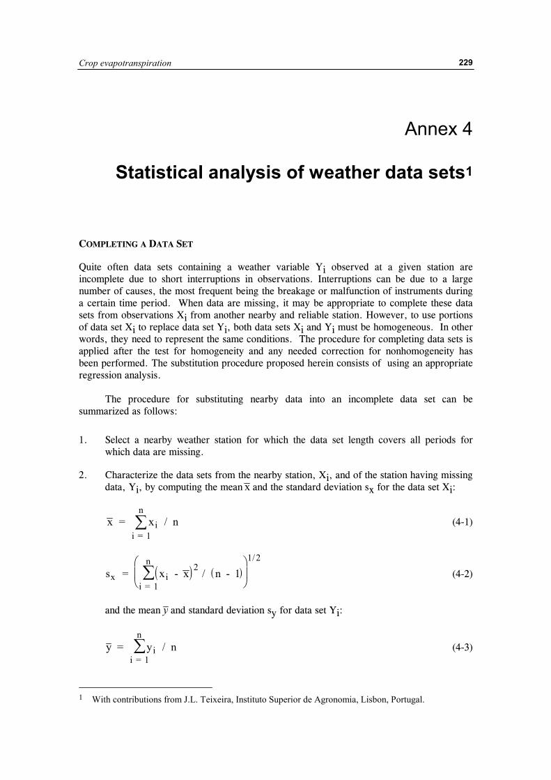
Crop evapotranspiration
229
Annex 4
Statistical analysis of weather data sets1
COMPLETING A DATA SET
Quite often data sets containing a weather variable Yi observed at a given station are incomplete due to short interruptions in observations. Interruptions can be due to a large number of causes, the most frequent being the breakage or malfunction of instruments during a certain time period. When data are missing, it may be appropriate to complete these data sets from observations Xi from another nearby and reliable station. However, to use portions of data set Xi to replace data set Yi, both data sets Xi and Yi must be homogeneous. In other words, they need to represent the same conditions. The procedure for completing data sets is applied after the test for homogeneity and any needed correction for nonhomogeneity has been performed. The substitution procedure proposed herein consists of using an appropriate regression analysis. The procedure for substituting nearby data into an incomplete data set can be summarized as follows:
1. Select a nearby weather station for which the data set length covers all periods for which data are missing.
2. Characterize the data sets from the nearby station, Xi, and of the station having missing data, Yi, by computing the mean x and the standard deviation sx for the data set Xi:
x = x / nii = 1
n� (4-1)
( ) ( )sx = x - x / n - 1i2
i = 1
n�
�
��
�
��
1 2/
(4-2)
and the mean y and standard deviation sy for data set Yi:
y = y / nii = 1
n� (4-3)
1 With contributions from J.L. Teixeira, Instituto Superior de Agronomia, Lisbon, Portugal.
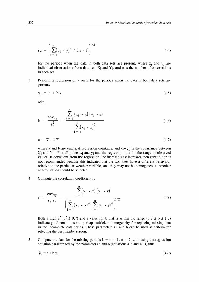
Annex 4: Statistical analysis of weather data sets
230
( ) ( )sy = y - y / n - 1i2
i = 1
n�
�
��
�
��
1 2/
(4-4)
for the periods when the data in both data sets are present, where xi and yi are individual observations from data sets Xi and Yi, and n is the number of observations in each set.
3. Perform a regression of y on x for the periods when the data in both data sets are present:
∃yi = a + b xi (4-5)
with
( ) ( )
( )b =
cov
s =
x - x y - y
x - x
xy
x2
i ii = 1
n
ii = 1
n
�
�2
(4-6)
a = y - b x (4-7)
where a and b are emprical regression constants, and covxy is the covariance between Xi and Yi. Plot all points xi and yi and the regression line for the range of observed values. If deviations from the regression line increase as y increases then substitution is not recommended because this indicates that the two sites have a different behaviour relative to the particular weather variable, and they may not be homogeneous. Another nearby station should be selected.
4. Compute the correlation coefficient r:
( ) ( )
( ) ( )r =
covs s
= x - x y - y
x - x y - y
xy
x y
i ii = 1
n
i ii = 1
n
i = 1
n
�
���
��
�
��
2 21 2/ (4-8)
Both a high r2 (r2 ≥ 0.7) and a value for b that is within the range (0.7 ≤ b ≤ 1.3) indicate good conditions and perhaps sufficient homogeneity for replacing missing data in the incomplete data series. These parameters r2 and b can be used as criteria for selecting the best nearby station.
5. Compute the data for the missing periods k = n + 1, n + 2..., m using the regression equation caracterized by the parameters a and b (equations 4-6 and 4-7), thus
k xb + a = ˆky (4-9)
Crop evapotranspiration
231
6. The complete data set with dimension m will now be
( )( )
Y
Y j
j
j
= y j = i = 1,..., n
= y = k = n + 1, n + 2,...,m
i
k∃ (4-10)
Note that estimates Yj = yk∃ taken from the regression equations are useful for predicting
evapotranspiration. However, they cannot be treated as random variables(2). ANALYSIS OF THE HOMOGENEITY OF DATA SERIES Weather data collected at a given weather station during a period of several years may be not homogeneous, i.e., the data set representing a particular weather variable may present a sudden change in its mean and variance in relation to the original values. This phenomenon may occur due to several causes, some of which are related to changes in instrumentation and observation practices, and others which relate to modification of the environmental conditions of the site, such as rapid urbanization or, on the contrary, perhaps development of irrigation in the area.
Changes relative to data collection may be caused by:
• change in type of sensor or instrument; • change in the observer and or change in the timing of observations; • “sleeping” data collector; • deterioration of sensors, such as with some types of pyranometers and RH sensors, or
malfunctionning of mechanical parts, such as with a tipping bucket rain gauge, or by an intermittently broken or shorted wire;
• aging of bearings on anemometers; • use of incorrect calibration coefficients; • variation in power supply or electronic behaviour of instruments; • growth of trees or planting of tall crops or construction of buildings or fences near a
raingauge, anemometer, or evaporation pan; • change in the location of the weather station, or in the types of shelters for housing
temperature and humidity sensors; • change in the watering, type or maintenance of vegetation in the vicinity of the weather
station; • significant change in the watering or type of vegetation of the region surrounding the
weather station. These changes cause observations made prior to the change to belong to a statistically different population than data collected after the change. It is therefore necessary to apply appropriate techniques to evaluate whether a given data set can be considered to be
22 To create random values,, one can add to ∃y k (equation 4-9) the residuals εk synthetically generated
from a population N (0, sy,x). The residuals are created using tables of random numbers. In that case the estimates Yj can be treated as random variables.
Annex 4: Statistical analysis of weather data sets
232
homogeneous and, if not, to introduce the appropriate corrections. To do so requires the identification of which sub-data series is to be corrected. To do this requires local information.
Procedures indicated herein are simple but are well proven in practice. They rely upon the statistical comparison of two data sets, one considered homogeneous and constituted by the observations Xi, the other being the one under analysis and consitutued by the observations Yi of the same weather variable (Tmax, Tmin, u2, RHmax,..., etc). Both sets Xi and Yi should be collected at two stations that are in the same climatic region, i. e., Xi and Yi should present the same trends in time despite the space variability when short time scales (daily, weekly or decadaily) are utilized.
The reference observations Xi are selected from a weather station for which the data set can be considered to be homogeneous.(3) The Xi data set should have the same time length of observations as the set of observations Yi.
Method of Cumulative Residuals
When relating two weather data sets from two weather stations, where the first is considered to be homogeneous, the data set of the second station can be considered to be homogeneous if the cumulative residuals of the second data set from a regression line based on the first data set are not biased. The bias hypothesis can be tested for a given probability p. This is done by verifying whether the residuals can be contained within an elipsis that has axis α and axis β. The magnitudes of α and β depend on the size of the data set, on the standard deviation of the sample being tested and on the probability p used to test the hypothesis(4).
The procedure for analysing the homogeneity of a weather data set Yi collected in a given weather station environment can be summarized as follows:
1. Select a reference weather station inside the same climatic region that is known to have an homogeneous data set Xi of the same weather variable. As an alternative, construct a “regional” homogeneous data set by averaging the observations at several weather stations in the same region.
2. Organize both data sets xi and yi in chronological order i = 1, 2,..., n, where the starting time and time increment are identical for both data sets.
3. For both data sets, compute the mean and standard deviation (equations 1 to 4) for the homogeneous variable (xi) and for the variable to be tested (yi).
3 When, for a given climatic region, there is no information concerning the homogeneity of data, then
the average of observations of the same variable from all stations (excluding the one in the analysis), Xi = � Xj, i / m, can be used to constitute the homogeneous data set.
4 This test utilizes results from residuals from the linear regression of Y on X. The residuals should follow a normal distribution with mean zero and standard deviation sy,x, i.e. the error εi ∈ N (0,sy,x). The residuals from the regression should be considered to be independent random variables (i.e., they should exhibit homoscedaticity).
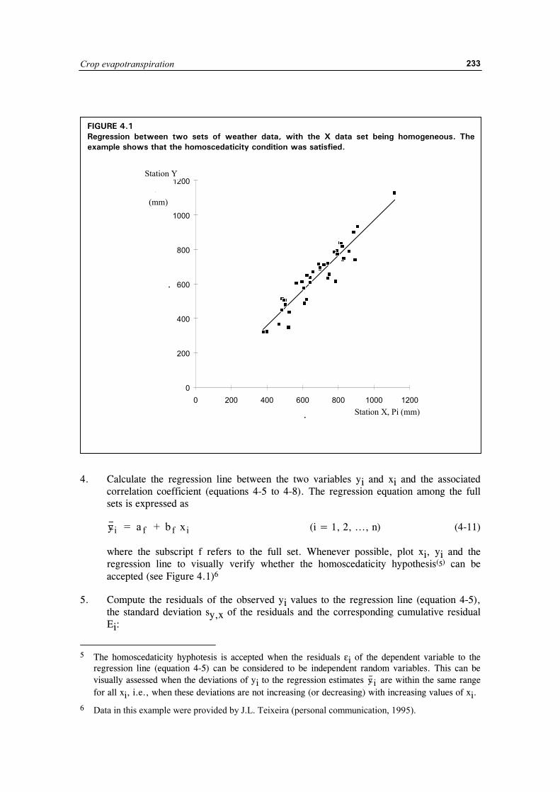
Crop evapotranspiration
233
4. Calculate the regression line between the two variables yi and xi and the associated correlation coefficient (equations 4-5 to 4-8). The regression equation among the full sets is expressed as
∃yi = a + b xf f i (i = 1, 2, ..., n) (4-11)
where the subscript f refers to the full set. Whenever possible, plot xi, yi and the regression line to visually verify whether the homoscedaticity hypothesis(5) can be accepted (see Figure 4.1)6
5. Compute the residuals of the observed yi values to the regression line (equation 4-5), the standard deviation sy,x of the residuals and the corresponding cumulative residual Ei:
5 The homoscedaticity hyphotesis is accepted when the residuals εi of the dependent variable to the
regression line (equation 4-5) can be considered to be independent random variables. This can be visually assessed when the deviations of yi to the regression estimates ∃yi are within the same range for all xi, i.e., when these deviations are not increasing (or decreasing) with increasing values of xi.
6 Data in this example were provided by J.L. Teixeira (personal communication, 1995).
FIGURE 4.1 Regression between two sets of weather data, with the X data set being homogeneous. Theexample shows that the homoscedaticity condition was satisfied.
0
200
400
600
800
1000
1200
0 200 400 600 800 1000 1200
.
.
Station Y
P(mm)
Station X, Pi (mm)
Annex 4: Statistical analysis of weather data sets
234
εi = y - yi i∃ (4-12)
( )sy,/
x y2 = s 1 - r
1 2 (4-13)
Ei = + i jj = 1
i - 1ε ε� ( )j i = ,... - 1 1 (4-14)
6. Select a probability p for accepting the hypothesis of homogeneity. The value p = 80% is commonly utilized. Then compute the elipsis equation having axes
α = n / 2 (4-15)
( )β = n
n - 1 z sp y, x1 2/ (4-16)
where: n size of the sample under analysis zp standard normal variate for the probability p (usually p = 80% for non
excedancy): Table 4.1 sy, x standard deviation of the residuals of y (equation 4-13)
The parametric equation of the elipsisis is then
( )( )
X
Y
= cos
= sin
α θ
β θ (4-17)
with θ [rad] varying from 0 to 2 π. Note: given the symmetry of the normal distribution, the values for p < 50% correspond to (100 - p) but with the opposite sign. Ex: p = 20% is associated with z = -z80 = -0.84
It can therefore be concluded, at the level of probability p, that there is no bias in the distribution of residuals, i.e., the data set yi is considered to be homogeneous, when the computed values for Ei fall inside the elipsis (equation 4-17).
7. Plot the cumulative residuals Ei against time using the time scale (interval) of the variable under analysis (Figure 4-2).
8. Draw the elipsis on the same plot and verify whether the Ei all lie inside the elipsis. If they do, then the hypothesis of homogeneity is accepted at the p level of confidence (Figure 4.4).
TABLE 4.1 Value of the standard normal variate zp for selected probabilities P of non-excedance
p (%) zp p (%) zp 50 60 70 75
0.00 0.25 0.52 0 67
80 85 90 95
0.84 1.04 1.28 1 64
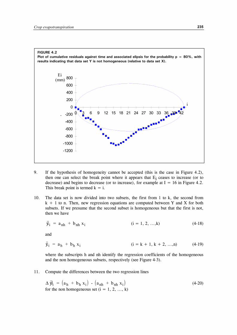
Crop evapotranspiration
235
9. If the hypothesis of homogeneity cannot be accepted (this is the case in Figure 4.2), then one can select the break point where it appears that Ei ceases to increase (or to decrease) and begins to decrease (or to increase), for example at I = 16 in Figure 4.2. This break point is termed k = i.
10. The data set is now divided into two subsets, the first from 1 to k, the second from k + 1 to n. Then, new regression equations are computed between Y and X for both subsets. If we presume that the second subset is homogeneous but that the first is not, then we have
∃yi = a + b xnh nh i (i = 1, 2, ...,k) (4-18)
and
∃yi = a + b xh h i (i = k + 1, k + 2, ...,n) (4-19)
where the subscripts h and nh identify the regression coefficients of the homogeneous and the non homogeneous subsets, respectively (see Figure 4-3).
11. Compute the differences between the two regression lines
( ) ( )∆ y = a + b x - a + b xi h h i nh nh i∃ (4-20) for the non homogeneous set (i = 1, 2, ..., k)
FIGURE 4.2 Plot of cumulative residuals against time and associated elipsis for the probability p = 80%, with results indicating that data set Y is not homogeneous (relative to data set X).
.
-1200
-1000
-800
-600
-400
-200
0
200
400
600
800
0 3 6 9 12 15 18 21 24 27 30 33 36 39 42
i
Ei(mm)
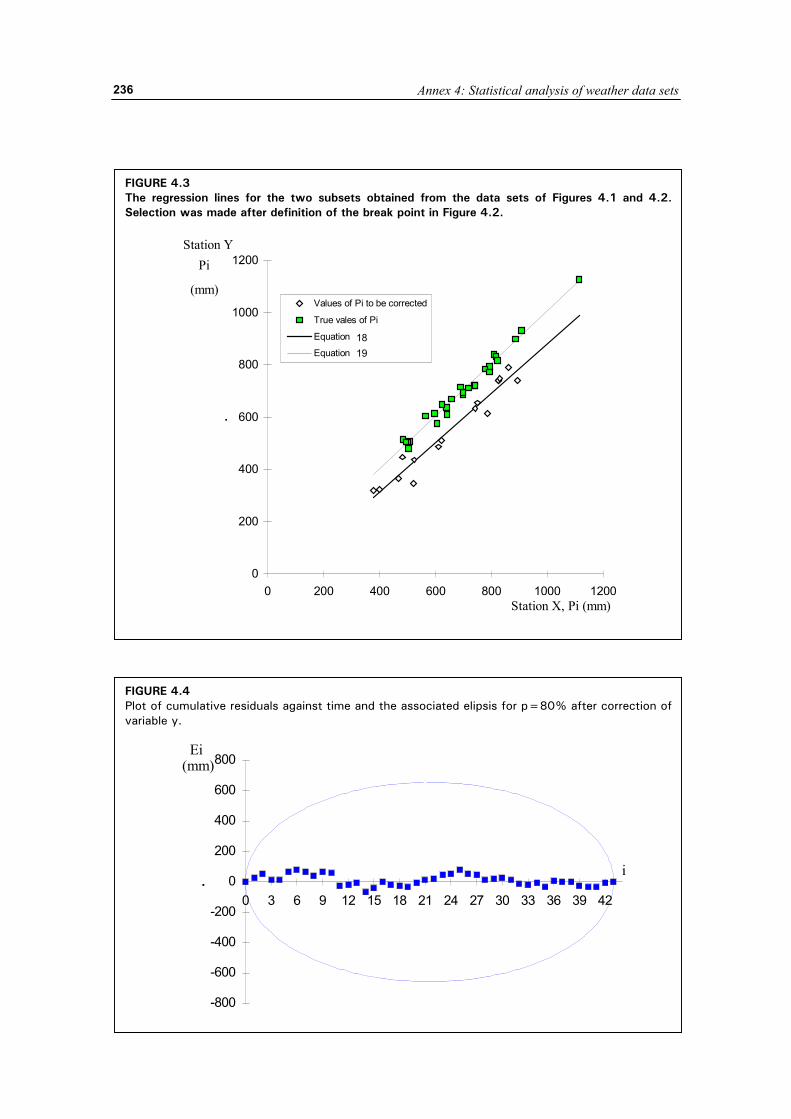
Annex 4: Statistical analysis of weather data sets
236
FIGURE 4.3 The regression lines for the two subsets obtained from the data sets of Figures 4.1 and 4.2. Selection was made after definition of the break point in Figure 4.2.
0
200
400
600
800
1000
1200
0 200 400 600 800 1000 1200
.
Values of Pi to be corrected
True vales of Pi
Equation 16
Equation 17
Station YPi
(mm)
Station X, Pi (mm)
1819
FIGURE 4.4 Plot of cumulative residuals against time and the associated elipsis for p=80% after correction of variable y.
.
-800
-600
-400
-200
0
200
400
600
800
0 3 6 9 12 15 18 21 24 27 30 33 36 39 42
i
Ei(mm)
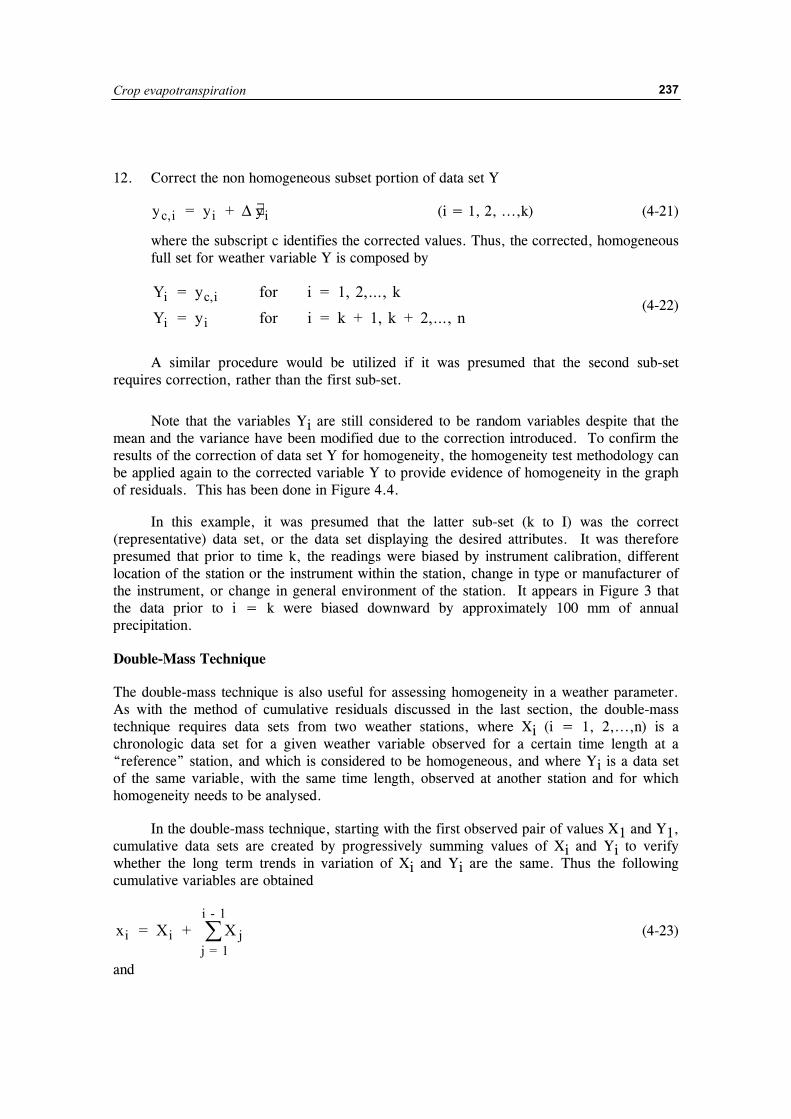
Crop evapotranspiration
237
12. Correct the non homogeneous subset portion of data set Y
yc i, ∃ = y + yi i∆ (i = 1, 2, ...,k) (4-21)
where the subscript c identifies the corrected values. Thus, the corrected, homogeneous full set for weather variable Y is composed by
Y for i for i
i = y = 1, 2,..., kY = y = k + 1, k + 2,..., n
c,i
i i (4-22)
A similar procedure would be utilized if it was presumed that the second sub-set requires correction, rather than the first sub-set.
Note that the variables Yi are still considered to be random variables despite that the mean and the variance have been modified due to the correction introduced. To confirm the results of the correction of data set Y for homogeneity, the homogeneity test methodology can be applied again to the corrected variable Y to provide evidence of homogeneity in the graph of residuals. This has been done in Figure 4.4.
In this example, it was presumed that the latter sub-set (k to I) was the correct (representative) data set, or the data set displaying the desired attributes. It was therefore presumed that prior to time k, the readings were biased by instrument calibration, different location of the station or the instrument within the station, change in type or manufacturer of the instrument, or change in general environment of the station. It appears in Figure 3 that the data prior to i = k were biased downward by approximately 100 mm of annual precipitation.
Double-Mass Technique
The double-mass technique is also useful for assessing homogeneity in a weather parameter. As with the method of cumulative residuals discussed in the last section, the double-mass technique requires data sets from two weather stations, where Xi (i = 1, 2,...,n) is a chronologic data set for a given weather variable observed for a certain time length at a “reference” station, and which is considered to be homogeneous, and where Yi is a data set of the same variable, with the same time length, observed at another station and for which homogeneity needs to be analysed.
In the double-mass technique, starting with the first observed pair of values X1 and Y1, cumulative data sets are created by progressively summing values of Xi and Yi to verify whether the long term trends in variation of Xi and Yi are the same. Thus the following cumulative variables are obtained
xi = X + Xi jj = 1
i - 1� (4-23)
and
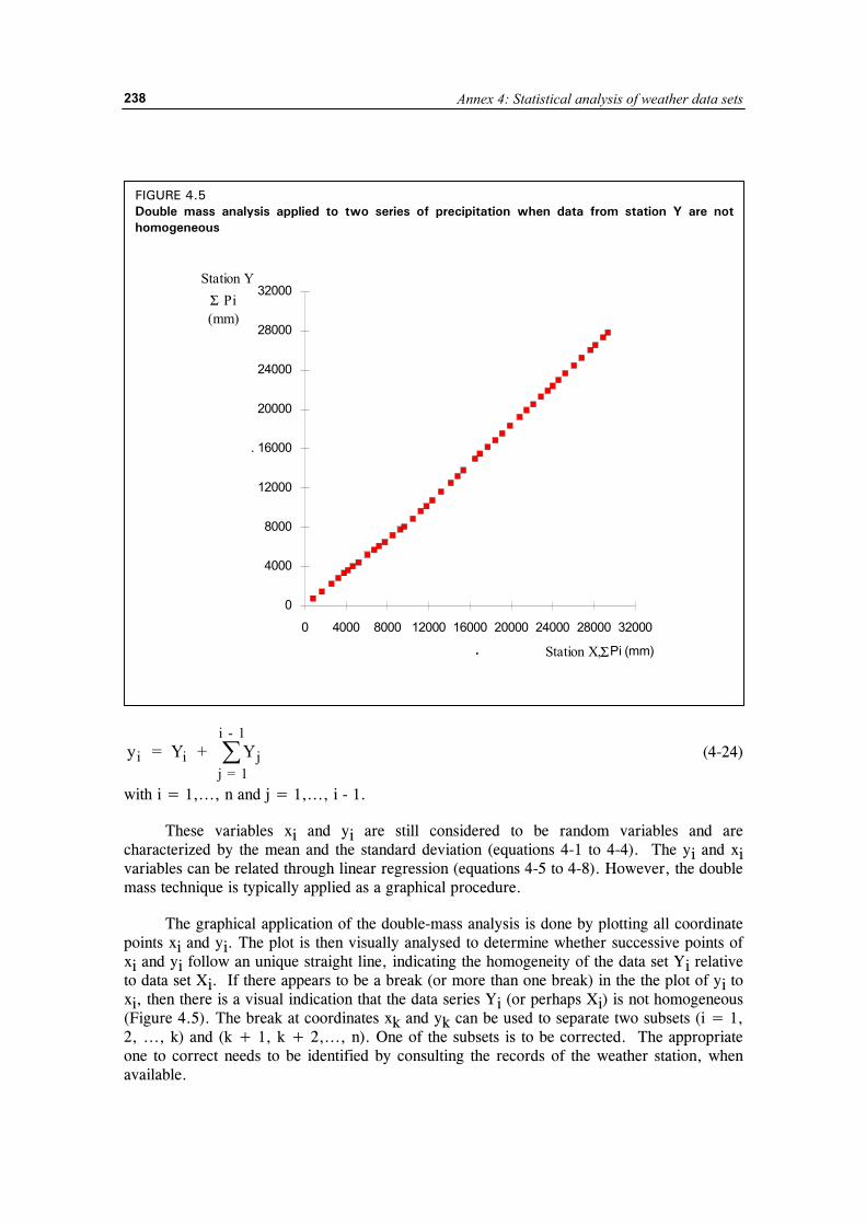
Annex 4: Statistical analysis of weather data sets
238
yi = Y + Yi jj = 1
i - 1� (4-24)
with i = 1,..., n and j = 1,..., i - 1.
These variables xi and yi are still considered to be random variables and are characterized by the mean and the standard deviation (equations 4-1 to 4-4). The yi and xi variables can be related through linear regression (equations 4-5 to 4-8). However, the double mass technique is typically applied as a graphical procedure.
The graphical application of the double-mass analysis is done by plotting all coordinate points xi and yi. The plot is then visually analysed to determine whether successive points of xi and yi follow an unique straight line, indicating the homogeneity of the data set Yi relative to data set Xi. If there appears to be a break (or more than one break) in the the plot of yi to xi, then there is a visual indication that the data series Yi (or perhaps Xi) is not homogeneous (Figure 4.5). The break at coordinates xk and yk can be used to separate two subsets (i = 1, 2, ..., k) and (k + 1, k + 2,..., n). One of the subsets is to be corrected. The appropriate one to correct needs to be identified by consulting the records of the weather station, when available.
FIGURE 4.5 Double mass analysis applied to two series of precipitation when data from station Y are nothomogeneous
.
.
0
4000
8000
12000
16000
20000
24000
28000
32000
0 4000 8000 12000 16000 20000 24000 28000 32000
Station YPi
(mm)
Station X,
Σ
ΣPi (mm)
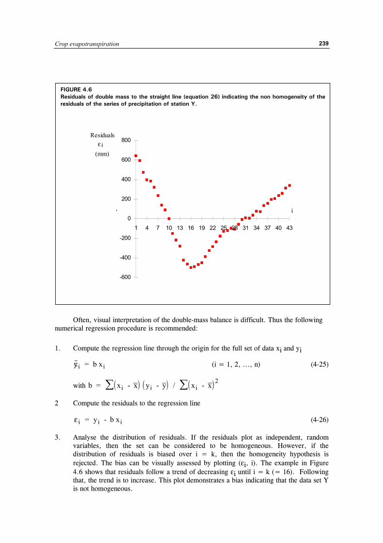
Crop evapotranspiration
239
Often, visual interpretation of the double-mass balance is difficult. Thus the following numerical regression procedure is recommended:
1. Compute the regression line through the origin for the full set of data xi and yi
∃yi = b xi (i = 1, 2, ..., n) (4-25)
with ( ) ( ) ( )b = x - x y - y / x - xi i i��2
2 Compute the residuals to the regression line
ε i = y - b xi i (4-26)
3. Analyse the distribution of residuals. If the residuals plot as independent, random variables, then the set can be considered to be homogeneous. However, if the distribution of residuals is biased over i = k, then the homogeneity hypothesis is rejected. The bias can be visually assessed by plotting (εi, i). The example in Figure 4.6 shows that residuals follow a trend of decreasing εi until i = k (= 16). Following that, the trend is to increase. This plot demonstrates a bias indicating that the data set Y is not homogeneous.
FIGURE 4.6 Residuals of double mass to the straight line (equation 26) indicating the non homogeneity of the residuals of the series of precipitation of station Y.
.
-600
-400
-200
0
200
400
600
800
1 4 7 10 13 16 19 22 25 28 31 34 37 40 43
i
(mm)
Residualsε i
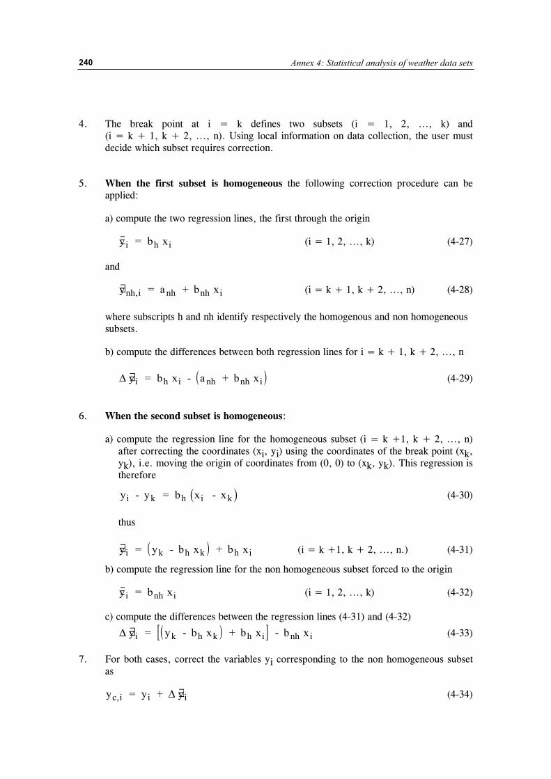
Annex 4: Statistical analysis of weather data sets
240
4. The break point at i = k defines two subsets (i = 1, 2, ..., k) and (i = k + 1, k + 2, ..., n). Using local information on data collection, the user must decide which subset requires correction.
5. When the first subset is homogeneous the following correction procedure can be applied:
a) compute the two regression lines, the first through the origin
∃yi = b xh i (i = 1, 2, ..., k) (4-27) and
∃ ,ynh i = a + b xnh nh i (i = k + 1, k + 2, ..., n) (4-28)
where subscripts h and nh identify respectively the homogenous and non homogeneous subsets.
b) compute the differences between both regression lines for i = k + 1, k + 2, ..., n
( )∆ y = b x - a + b x i h i nh nh i∃ (4-29)
6. When the second subset is homogeneous:
a) compute the regression line for the homogeneous subset (i = k +1, k + 2, ..., n) after correcting the coordinates (xi, yi) using the coordinates of the break point (xk, yk), i.e. moving the origin of coordinates from (0, 0) to (xk, yk). This regression is therefore
( )yi - y = b x - xk h i k (4-30)
thus
( )∃yi = y - b x + b xk h k h i (i = k +1, k + 2, ..., n.) (4-31)
b) compute the regression line for the non homogeneous subset forced to the origin
∃yi = b xnh i (i = 1, 2, ..., k) (4-32)
c) compute the differences between the regression lines (4-31) and (4-32)
( )[ ]∆ y = y - b x + b x - b xi k h k h i nh i∃ (4-33)
7. For both cases, correct the variables yi corresponding to the non homogeneous subset as
yc i, ∃ = y + yi i∆ (4-34)
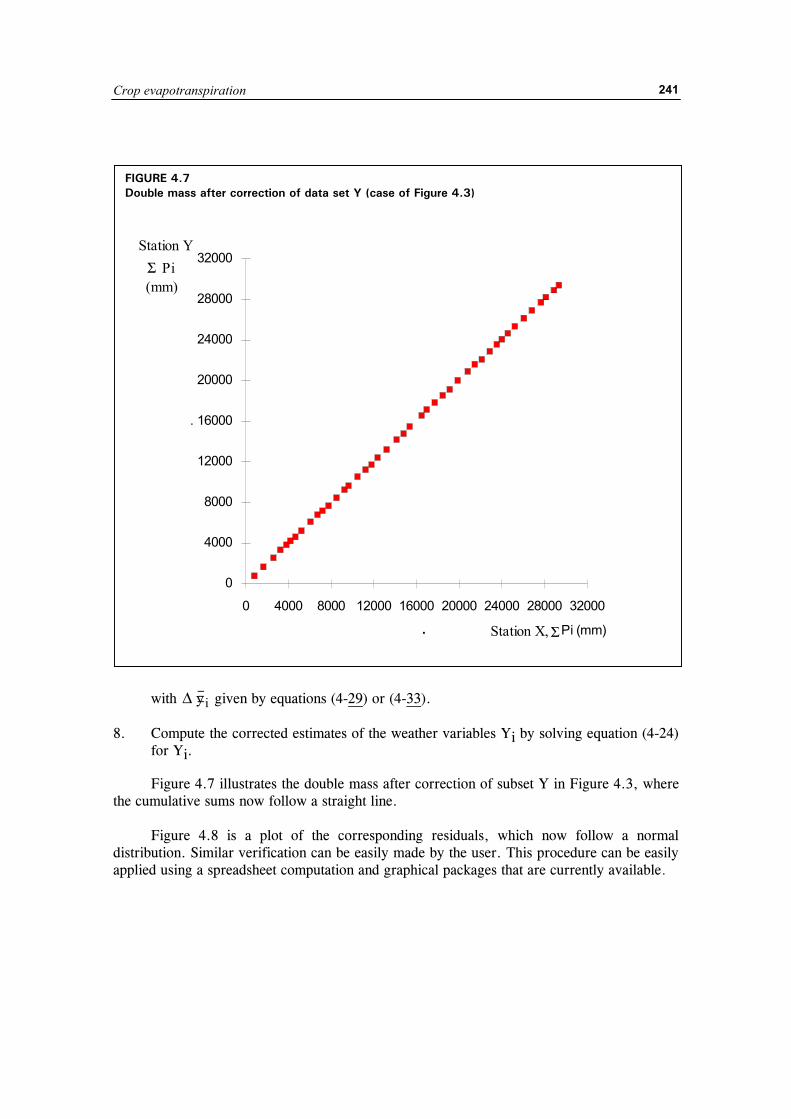
Crop evapotranspiration
241
with ∆ yi∃ given by equations (4-29) or (4-33).
8. Compute the corrected estimates of the weather variables Yi by solving equation (4-24) for Yi.
Figure 4.7 illustrates the double mass after correction of subset Y in Figure 4.3, where the cumulative sums now follow a straight line. Figure 4.8 is a plot of the corresponding residuals, which now follow a normal distribution. Similar verification can be easily made by the user. This procedure can be easily applied using a spreadsheet computation and graphical packages that are currently available.
FIGURE 4.7 Double mass after correction of data set Y (case of Figure 4.3)
.
.
0
4000
8000
12000
16000
20000
24000
28000
32000
0 4000 8000 12000 16000 20000 24000 28000 32000
Station YPi
(mm)
Station X,
Σ
ΣPi (mm)
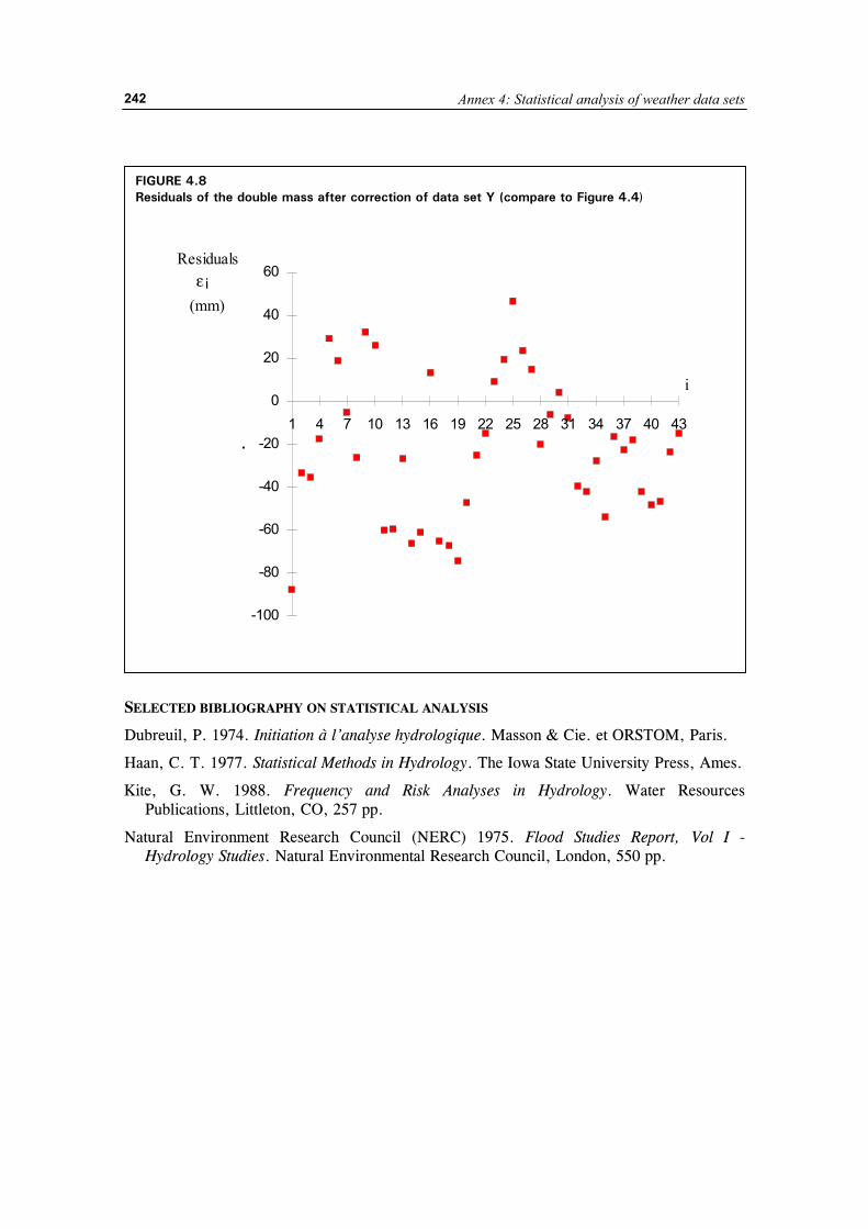
Annex 4: Statistical analysis of weather data sets
242
SELECTED BIBLIOGRAPHY ON STATISTICAL ANALYSIS
Dubreuil, P. 1974. Initiation à l’analyse hydrologique. Masson & Cie. et ORSTOM, Paris.
Haan, C. T. 1977. Statistical Methods in Hydrology. The Iowa State University Press, Ames.
Kite, G. W. 1988. Frequency and Risk Analyses in Hydrology. Water Resources Publications, Littleton, CO, 257 pp.
Natural Environment Research Council (NERC) 1975. Flood Studies Report, Vol I - Hydrology Studies. Natural Environmental Research Council, London, 550 pp.
FIGURE 4.8 Residuals of the double mass after correction of data set Y (compare to Figure 4.4)
.
-100
-80
-60
-40
-20
0
20
40
60
1 4 7 10 13 16 19 22 25 28 31 34 37 40 43
i
(mm)
Residualsε i
Crop evapotranspiration
243
NOTATION IN STATISTICAL ANALYSIS
a regression coefficient
b regression coefficient
covxy covariance of variables x and y
Ei cumulative residuals
i number of order of variable xi in the sample
j, k number of a variable in a subset
n size of the sample
p probability
p (x) probability distribution density function
r correlation coefficient
r2 coefficient of determination
sx estimate of the standard deviation of the variable x
sx2 estimate of the variance of the variable x
sy estimate of the standard deviation of the variable y
sy2 estimate of the variance of the variable y
sy,x standard deviation of the residuals of y estimated from the regression
X random variable
Xi value of a variable in a data set
xi random variable
∃xp estimated value for the variable x with probability of non excedance p
x estimate of the mean, or mean of a sample of the random variable xi
Y transformed variable from X
Yi value of a variable in a data set
yi random variable
∃yi value of yi estimated from the regression
y estimate of the mean, or mean of a sample of the random variable yi
Z standard normal variable
zp value of the standard normal variable for the probability p
εi residuals of y estimated from the regression
µ mean of a population
σ standard deviation of a population

Annex 4: Statistical analysis of weather data sets
244
Crop evapotranspiration
245
Annex 5
Measuring and assessing integrity of weather data
Estimates of reference evapotranspiration (ETo) are no better than weather data upon which they are based. Assessments of weather data integrity and quality need to be conducted before data are utilized in ETo equations. When necessary and when possible, corrections to the data should be made to account for poor sensor calibration. Some of these corrections are described in section 1 of Annex 4.
A good cautionary statement in data analysis and application is that “no data are better than bad data.” This statement applies primarily to measurements of evapotranspiration that are used to develop or to calibrate reference ET equations or to determine crop coefficients. However, it also applies to weather data. When one has no data, one can look to regional weather or ET data summaries for information that might be useful to represent conditions within the local area. In the case of ET data, one might go to a publication such as this one to make reasonably accurate estimates of ETo and ETc. However, in the case of “bad” data, meaning biased, or faulty, or nonrepresentative data collected locally, one is “stuck” with weather data and associated predictions of ETo and ETc, or with local measurements of ETc that can be biased, faulty, or nonrepresentative. The result is application of evapotranspiration data or evapotranspiration calculations to irrigation water management, to water resources operations, or to irrigation and water resources systems design that can actually cause more economic and hydrologic problems than if only reasonable estimates or even “textbook” values for ETc had been used instead. Humanity can be worse off because of faulty data as compared to no data.
Some years ago, when computer modeling was in its infancy, a common cautionary advice was to “do not trust any model until it has been validated using independent data.” Today, with some of the more common mathematical models becoming proven and trustworthy, the corollary of this expression is commonly advocated, where “one should not trust any data until they are validated using a model!” Certainly, some place in between these two cautionary advocations is appropriate. Often a valid model can be valuable for evaluating data to identify errors, outliers and biases. And of course, valid data are required for selecting or calibrating a particular model.
This Annex presents guidelines to be used to calculate both extreme ranges for weather data measurements and also means to assess integrity of data that fall between the extremes. A review on instrumentation for agricultural weather stations is given first.
Annex 5: Measuring and assessing integrity of weather data
246
INSTRUMENTATION FOR MEASURING WEATHER VARIABLES1
Data Acquisition and Instrumentation
Radiation
Solar radiation is commonly measured with pyranometers. Pyranometers measure the shortwave incoming radiation in a solid angle in the shape of a hemisphere oriented upwards. Currently, in the most common “glassed dome” pyranometers, a thermopile is used within the instrument as the sensor, where thermal gradients are measured across hot and cold areas (black and white). The radiation intensity is proportional to the temperature differences between the two sensing areas. Accuracy depends upon the sensitivity of the material used in the sensors, the response time and the distortion characteristics of the material constituting the dome covering the sensors. A second type of pyranometer that is less expensive and that is gaining acceptance is the silicon diode instrument where electric current is generated by a photo sensitive diode in proportion to solar intensity. Ordinarily, silicon diode pyranometers are not fully sensitive to the full spectrum of visible light, so that the calibration of the instrument is only valid for upward solar measurements.
When a pyranometer is oriented downwards it measures the reflected shortwave radiation, and is thus called an albedometer. When two pyranometers are associated, one oriented upwards and the other downwards, the net short wave radiation is measured. The instrument is then called a net pyranometer. A point of caution is that any instrument used as an albedometer or net pyranameter must have full sensitivity to all spectra of visible light. This is important since the composition of reflected light from vegetation is highly biased toward green. Therefore, most albedometers must be of the glass domed thermopile type and not the photo diode type.
Net radiation is measured by pyradiometers (or net radiometers), which sense both short and long wave radiation. They have two bodies, one oriented upwards and the other downwards, both covering a solid angle in the shape of a hemisphere. The sensors are made from several thermocouples sensing heat generated by radiation from all wavelengths, and are protected by domes made in general of polyethylene treated in a specific manner. The black bodies can loose their sensing capabilities with time, so that these instruments require regular and frequent calibrations. Other net radiometers are comprised of ventilated differential thermopiles, but they are very seldom utilized. All radiometers refered to above transform the radiation energy into thermal energy, a portion of which is transformed into an electric voltage gradient that provides appropriate conditions for continuous recording using dataloggers.
Sunshine duration is most commonly recorded with the Campbell-Stokes heliograph. A glass globe focuses the radiation beam to a special recording paper and a trace is burned on the paper as the sun is moving. No records occur when no bright sunshine is sensed. Measurements are reliable when the recording paper is placed in the right position according to the relative position of the sun. Care is required to avoid accumulation of rain water on the paper. The heliograph has to be oriented South in the northern hemisphere and North in the
1 Details on weather station instrumentation can be found in FAO 27 (Doorenbos, 1976), in the WMO
Guide to Agrometeorological Practices (WMO, 1981, 1983), or in meteorology handbooks (Seemann et al., 1979; Rosenberg et al., 1983; Kessler et al., 1990).
Crop evapotranspiration
247
southern hemisphere. In China, another type of heliograph is used. The solar beam penetrates through an orifice and traces a recording paper treated with a sensible chemical substance. Electronic records of sunshine duration are obtained through the photo-electric or the rotating optical fibre sunshine recorders.
Windspeed
Windspeed is measured using anemometers, always placed at an height not less than 2 m above the ground, and often at 5 m, following recommendations by WMO. Most common are the three-cup anemometers. Also common are propeller anemometers. Measurements by both types are reliable provided that maintenance ensures appropriate functioning of the mechanical parts. Older designs of anemometers utilize mechanical counters as the output device. Modern anemometers may be equipped with generators giving a voltage signal that is proportional to the windspeed. Other anemometers may be equipped with small magnetic reed switches or with opto-electronic couplers that generate electric impulses in proportion to the windspeed. The electronic devices are utilized in automatic weather stations. Accuracy of windspeed measurements depends on the upwind fetch as much as on instrumentation. A large upwind fetch that is free of buildings and trees is definitely required for representative measurements. Temperature
The most commonly utilized sensor for measuring temperature are still the mercury thermometers. Maximum and minimum thermometers use mercury and alcohol. Bimetallic thermographs are the most common mechanical temperature recorders. They are easy to read and maintain. However, mechanical thermographs do require verification and adjustment of the position of the pen recorder. These instruments are installed in shelters that are naturally ventilated.
Modern temperature sensors have been developed, namely the thermistor and the thermocouple. These provide very accurate analogue measurements and are normally utilized in automatic weather stations. Thermistors provide independent measurements of air or soil temperature, whereas thermocouples require an additional base temperature reading, normally provided by a thermistor. To maintain the accuracy and representativeness of these instruments, they are installed in special radiation shields (shelters) having natural ventilation. Occasionally the shields or shelters are artificially aspirated to reduce biases caused by heat loading from the sun. Humidity
Dew point temperature is often measured with a mirrorlike metallic surface that is artificially cooled. When dew forms on the surface, its temperature is sensed as Tdew. Other dew sensor systems use chemical or electric properties of certain materials that are altered when absorbing water vapour. Instruments for measuring dew point temperature require careful operation and maintenance and are seldom available in weather stations. The accuracy of estimation of the actual vapour pressure from Tdew is generally very high.
Relative humidity is measured using hygrometers. Most frequently used in mechanically-based field stations are the hair hygrometers, normally operated as mechanical hygrographs. Measurements loose accuracy with dust and ageing of the hairs. Modern hygrometers use a film from a dielectric polymer that changes its dielectric constant with
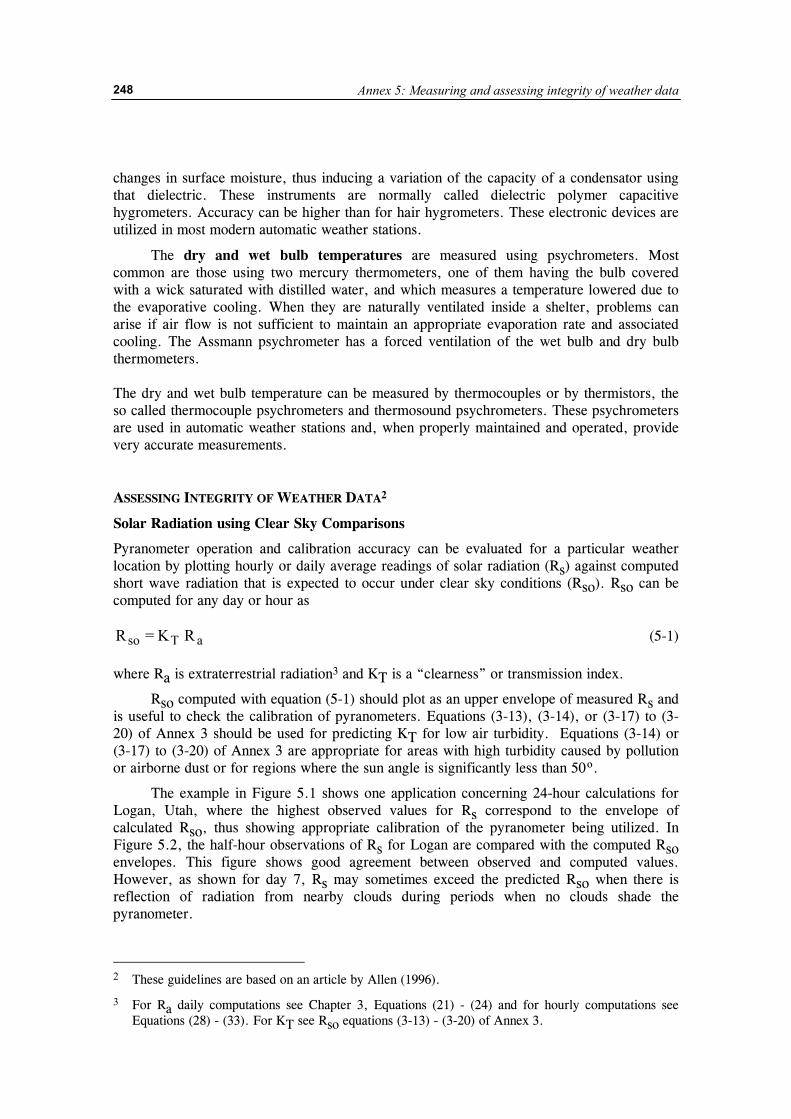
Annex 5: Measuring and assessing integrity of weather data
248
changes in surface moisture, thus inducing a variation of the capacity of a condensator using that dielectric. These instruments are normally called dielectric polymer capacitive hygrometers. Accuracy can be higher than for hair hygrometers. These electronic devices are utilized in most modern automatic weather stations.
The dry and wet bulb temperatures are measured using psychrometers. Most common are those using two mercury thermometers, one of them having the bulb covered with a wick saturated with distilled water, and which measures a temperature lowered due to the evaporative cooling. When they are naturally ventilated inside a shelter, problems can arise if air flow is not sufficient to maintain an appropriate evaporation rate and associated cooling. The Assmann psychrometer has a forced ventilation of the wet bulb and dry bulb thermometers. The dry and wet bulb temperature can be measured by thermocouples or by thermistors, the so called thermocouple psychrometers and thermosound psychrometers. These psychrometers are used in automatic weather stations and, when properly maintained and operated, provide very accurate measurements. ASSESSING INTEGRITY OF WEATHER DATA2
Solar Radiation using Clear Sky Comparisons
Pyranometer operation and calibration accuracy can be evaluated for a particular weather location by plotting hourly or daily average readings of solar radiation (Rs) against computed short wave radiation that is expected to occur under clear sky conditions (Rso). Rso can be computed for any day or hour as
aTso R K = R (5-1)
where Ra is extraterrestrial radiation3 and KT is a “clearness” or transmission index.
Rso computed with equation (5-1) should plot as an upper envelope of measured Rs and is useful to check the calibration of pyranometers. Equations (3-13), (3-14), or (3-17) to (3-20) of Annex 3 should be used for predicting KT for low air turbidity. Equations (3-14) or (3-17) to (3-20) of Annex 3 are appropriate for areas with high turbidity caused by pollution or airborne dust or for regions where the sun angle is significantly less than 50º.
The example in Figure 5.1 shows one application concerning 24-hour calculations for Logan, Utah, where the highest observed values for Rs correspond to the envelope of calculated Rso, thus showing appropriate calibration of the pyranometer being utilized. In Figure 5.2, the half-hour observations of Rs for Logan are compared with the computed Rso envelopes. This figure shows good agreement between observed and computed values. However, as shown for day 7, Rs may sometimes exceed the predicted Rso when there is reflection of radiation from nearby clouds during periods when no clouds shade the pyranometer.
2 These guidelines are based on an article by Allen (1996). 3 For Ra daily computations see Chapter 3, Equations (21) - (24) and for hourly computations see
Equations (28) - (33). For KT see Rso equations (3-13) - (3-20) of Annex 3.
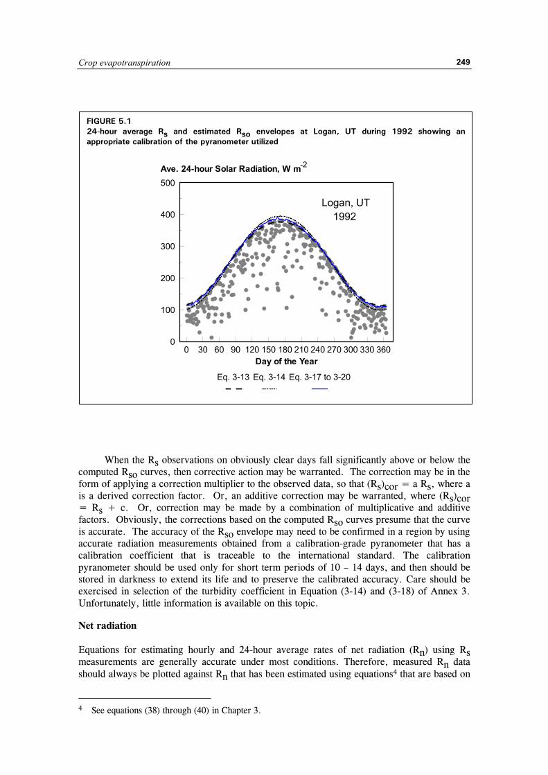
Crop evapotranspiration
249
When the Rs observations on obviously clear days fall significantly above or below the computed Rso curves, then corrective action may be warranted. The correction may be in the form of applying a correction multiplier to the observed data, so that (Rs)cor = a Rs, where a is a derived correction factor. Or, an additive correction may be warranted, where (Rs)cor = Rs + c. Or, correction may be made by a combination of multiplicative and additive factors. Obviously, the corrections based on the computed Rso curves presume that the curve is accurate. The accuracy of the Rso envelope may need to be confirmed in a region by using accurate radiation measurements obtained from a calibration-grade pyranometer that has a calibration coefficient that is traceable to the international standard. The calibration pyranometer should be used only for short term periods of 10 – 14 days, and then should be stored in darkness to extend its life and to preserve the calibrated accuracy. Care should be exercised in selection of the turbidity coefficient in Equation (3-14) and (3-18) of Annex 3. Unfortunately, little information is available on this topic. Net radiation Equations for estimating hourly and 24-hour average rates of net radiation (Rn) using Rs measurements are generally accurate under most conditions. Therefore, measured Rn data should always be plotted against Rn that has been estimated using equations4 that are based on 4 See equations (38) through (40) in Chapter 3.
FIGURE 5.1 24-hour average Rs and estimated Rso envelopes at Logan, UT during 1992 showing an appropriate calibration of the pyranometer utilized
-2
Logan, UT 1992
0 30 60 90 120 150 180 210 240 270 300 330 3600
100
200
300
400
500
Day of the Year
Ave. 24-hour Solar Radiation, W m
Eq. 3-13 Eq. 3-14 Eq. 3-17 to 3-20
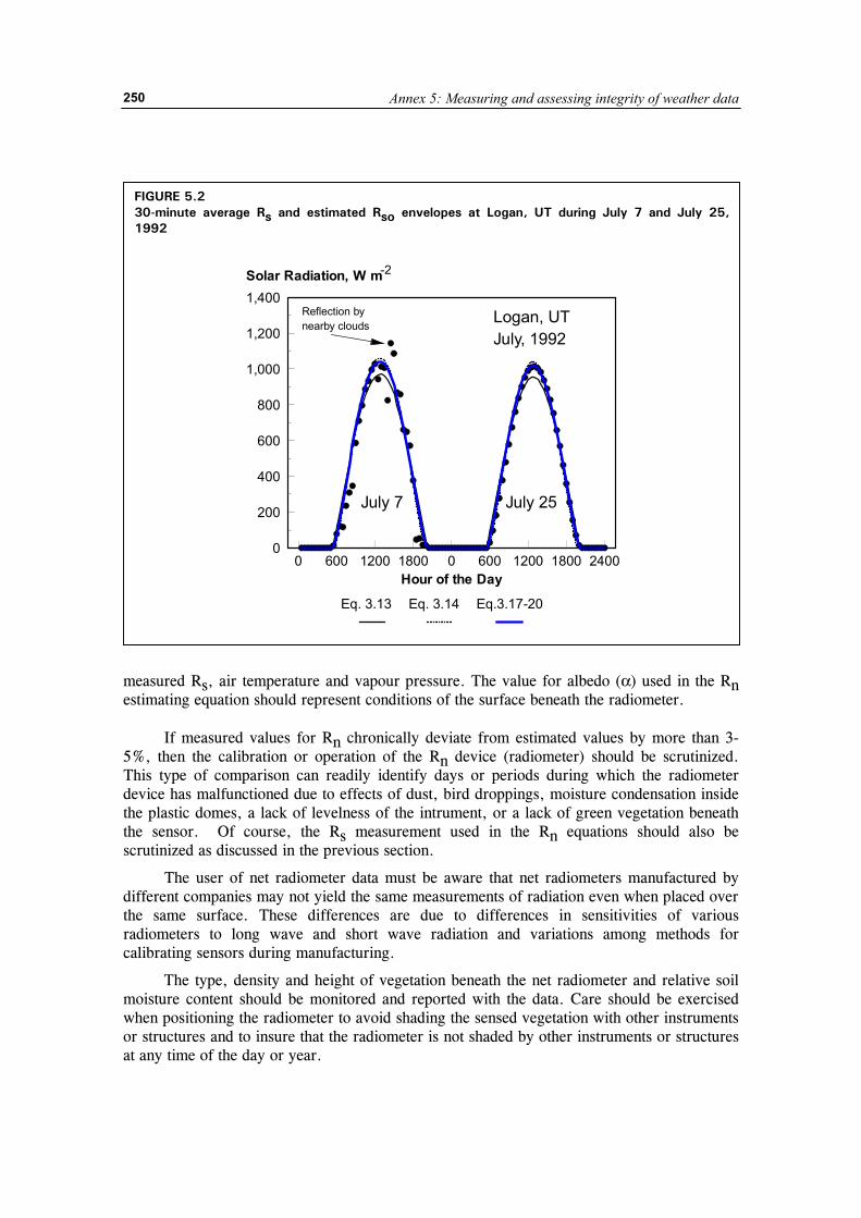
Annex 5: Measuring and assessing integrity of weather data
250
measured Rs, air temperature and vapour pressure. The value for albedo (α) used in the Rn estimating equation should represent conditions of the surface beneath the radiometer. If measured values for Rn chronically deviate from estimated values by more than 3-5%, then the calibration or operation of the Rn device (radiometer) should be scrutinized. This type of comparison can readily identify days or periods during which the radiometer device has malfunctioned due to effects of dust, bird droppings, moisture condensation inside the plastic domes, a lack of levelness of the intrument, or a lack of green vegetation beneath the sensor. Of course, the Rs measurement used in the Rn equations should also be scrutinized as discussed in the previous section.
The user of net radiometer data must be aware that net radiometers manufactured by different companies may not yield the same measurements of radiation even when placed over the same surface. These differences are due to differences in sensitivities of various radiometers to long wave and short wave radiation and variations among methods for calibrating sensors during manufacturing.
The type, density and height of vegetation beneath the net radiometer and relative soil moisture content should be monitored and reported with the data. Care should be exercised when positioning the radiometer to avoid shading the sensed vegetation with other instruments or structures and to insure that the radiometer is not shaded by other instruments or structures at any time of the day or year.
FIGURE 5.2 30-minute average Rs and estimated Rso envelopes at Logan, UT during July 7 and July 25, 1992
-2
Logan, UTJuly, 1992
July 7 July 25
Reflection bynearby clouds
0 600 1200 1800 0 600 1200 1800 24000
200
400
600
800
1,000
1,200
1,400
Hour of the Day
Solar Radiation, W m
Eq. 3.13 Eq. 3.14 Eq.3.17-20
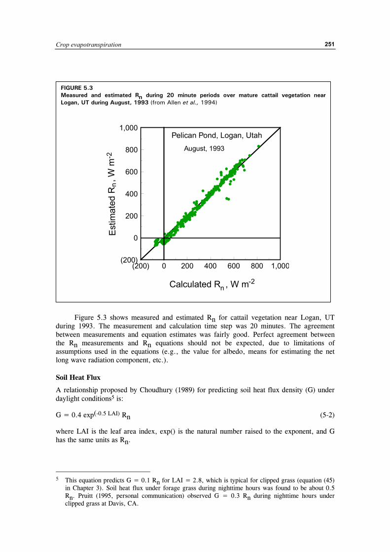
Crop evapotranspiration
251
Figure 5.3 shows measured and estimated Rn for cattail vegetation near Logan, UT during 1993. The measurement and calculation time step was 20 minutes. The agreement between measurements and equation estimates was fairly good. Perfect agreement between the Rn measurements and Rn equations should not be expected, due to limitations of assumptions used in the equations (e.g., the value for albedo, means for estimating the net long wave radiation component, etc.). Soil Heat Flux
A relationship proposed by Choudhury (1989) for predicting soil heat flux density (G) under daylight conditions5 is:
G = 0.4 exp(-0.5 LAI) Rn (5-2)
where LAI is the leaf area index, exp() is the natural number raised to the exponent, and G has the same units as Rn.
5 This equation predicts G = 0.1 Rn for LAI = 2.8, which is typical for clipped grass (equation (45)
in Chapter 3). Soil heat flux under forage grass during nighttime hours was found to be about 0.5 Rn. Pruitt (1995, personal communication) observed G = 0.3 Rn during nighttime hours under clipped grass at Davis, CA.
FIGURE 5.3 Measured and estimated Rn during 20 minute periods over mature cattail vegetation nearLogan, UT during August, 1993 (from Allen et al., 1994)
(200) 0 200 400 600 800 1,000(200)
0
200
400
600
800
1,000
Calculated R , W m-2n
Estim
ated
R ,
W m
-2n
Pelican Pond, Logan, UtahAugust, 1993
Annex 5: Measuring and assessing integrity of weather data
252
Equation (5-2) can be used to check the functioning and relative accuracy of soil heat flux plates after correcting measurements for temperature change of soil above the plates. The relationship of Equation (5-2) does not hold for 24-hour data, as a positive 24-hour soil heat flux estimate would always result. The user must be aware that Eq. (5-2) is only approximate and does not consider effects of plant spacing, sun angle, soil colour, soil moisture, or soil texture, nor the sensible heat balance at the surface on the ratio of G to Rn. Generally, more than one soil heat flux plate is used due to spatial variation in soil, soil water content, and vegetation.
Windspeed
Accuracy of wind measurements is difficult to assess unless duplicate instruments are used. One should always scan wind records for the presence of consistently low wind recordings. For electronic instruments, these recordings may represent a numerical “offset” in the anemometer calibration equation. The presence of these constant and consistent offsets in the data set indicates either the presence of exceptionally calm conditions (wind speeds less than about 0.5 m s-1 during the entire sampling period (which is rare)) or a malfunctioning of the wind speed sensor due to electrical shorting or perhaps due to fatigue of bearings. These problems may not be noticed by the station operator.
When possible, a second anemometer6 of the same design, but with fresh bearings, should be placed at the weather location for a three or four day period at least once each year, and recordings compared with the permanent instrument. Variations between recordings can signal a need to replace bearings, switches, or other parts.
Relative Humidity and Vapour Pressure
Vapour pressure of air is difficult to measure accurately. Some older electronic humidity sensors were commonly plagued by hysteresis, nonlinearity and calibration errors. Some of these errors are inherent in the sensor design and still plague some modern sensors. Other errors result from dust, moisture, insects, pollution, and age. Replication of RH Instruments
It is strongly recommended that duplicate RH and air temperature sensors be permanently employed in electronic weather stations, at least for some period each year. When duplicate RH and air temperature sensors yield similar measurments, then it is likely that both sensors are functioning properly, provided proper calibration equations have been used. However, even though duplicate sensors are in agreement does not mean that the readings are free from calibration errors and biases due to nonlinearity, etc.. Trends in Computed Dew Point Temperature with Time
When air humidity is measured using RH sensors, the actual vapour pressure of the air (ea) is calculated as:
6 If a second data logger is used to record the temporary anemometer, one should be careful to
synchronize data logger clocks. Also, one should be careful that anemometers do not interfere with one another’s wind stream.
Crop evapotranspiration
253
( )T eº 100RH = ae (5-3)
where eº (T) is the saturation vapour pressure at air temperature T and RH is in %. RH and T must be taken for the same time period, preferably for ≤ 1 hour .
Hourly (or shorter) measurements of RH, dew point temperature (Tdew) or vapour pressure (ea) can be preliminarily assessed by plotting hourly measurements of computed Tdew or ea with time. Relative humidity will vary significantly with time of day, and inversely with air temperature as shown in Figure 12 of Chapter 3. However, both Tdew and ea, either measured directly, or computed using RH and T measurements, should remain somewhat constant throughout a 24-hour period when the air mass is stable and advection of dry air from outside the area does not occur. During these stable periods, one should expect some rise in Tdew and ea during daytime periods, when ET fluxes humidify the equilibrium boundary layer. However, this increase is usually less than about 10 to 20%. Variation in Tdew increases significantly when a weather front passes overhead. Since ea is calculated as the product of RH and saturation vapour pressure at air temperature, any error in the RH calibration tends to cause false variation in Tdew and ea with changing air temperature.
Figure 5.4 shows Tdew computed from measurements of RH and air temperature at a weather station in the center of a wetland near Logan, UT (20-minute data). Tdew generally varied from hour to hour due to air mass instability and increased during most days of this period as evaporation from the local wetland vegetation added humidity to the air. The data sequence shows some periods of relatively constant measurement (calculation) of Tdew throughout a 24-hour period (for example day of year 199), even though air temperature varied substantially. This is a good indication that the RH sensor was probably functioning correctly and that the instrument calibrations were probably valid.
Figure 5.4 also shows, for the same weather station, a comparison between RH measured using two different and independent relative humidity sensors. The two sensors, one a “chilled-mirror” device that measures Tdew directly, and the other, a device that measures RH directly, agreed very well with each other during the 8 days shown. The value of having “redundancy” in instrumentation is demonstrated in this example, where the two different devices measuring the same parameter (in this case RH) leave no question concerning the validity and accuracy of the RH measurements, due to the close agreement. The use of only a single instrument would leave some question as to accuracy.
One can notice in Figure 5.4 that the RH approached 100% on day 200, which is expected for a well-watered setting. The difference between minimum daily temperature and Tdew was generally 1 to 2 oC for many of the days. This is expected in dry, advective environments, as discussed in Chapter 3 and Annex 6. Observations During Periods of Dew and Rainfall
In many climates, especially those where nightime dew occurs, Td during early morning hours before sunrise should coincide closely with recorded Tmin and RH should approach 100%. For automatic recording weather stations where recording rain gauges are used, one should expect RH recordings during periods of rain or light drizzle to exceed 95%. Relative humidity recordings that exceed 100% by more than 3-5% during early morning hours or during precipitation events indicate a need for recalibration and numerical adjustment of collected data.
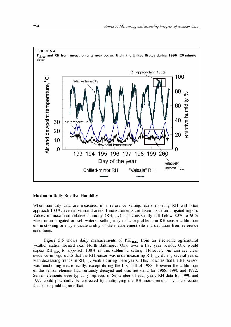
Annex 5: Measuring and assessing integrity of weather data
254
Maximum Daily Relative Humidity
When humidity data are measured in a reference setting, early morning RH will often approach 100%, even in semiarid areas if measurements are taken inside an irrigated region. Values of maximum relative humidity (RHmax) that consistently fall below 80% to 90% when in an irrigated or well-watered setting may indicate problems in RH sensor calibration or functioning or may indicate aridity of the measurement site and deviation from reference conditions.
Figure 5.5 shows daily measurements of RHmax from an electronic agricultural weather station located near North Baltimore, Ohio over a five year period. One would expect RHmax to approach 100% in this subhumid setting. However, one can see clear evidence in Figure 5.5 that the RH sensor was undermeasuring RHmax during several years, with decreasing trends in RHmax visible during these years. This indicates that the RH sensor was functioning electronically, except during the first half of 1988. However the calibration of the sensor element had seriously decayed and was not valid for 1988, 1990 and 1992. Sensor elements were typically replaced in September of each year. RH data for 1990 and 1992 could potentially be corrected by multiplying the RH measurements by a correction factor or by adding an offset.
FIGURE 5.4 Tdew and RH from measurements near Logan, Utah, the United States during 1995 (20-minute data)
193 194 195 196 197 198 199 2000
1020304050607080
0
20
40
60
80
100
Day of the year
Chilled-mirror RH "Vaisala" RH
Air a
nd d
ewpo
int t
empe
ratu
re,
Co
Rel
ativ
e hu
mid
ity, %
dewpoint temperature
air temperature
relative humidity
RelativelyUniform Tdew
RH approaching 100%
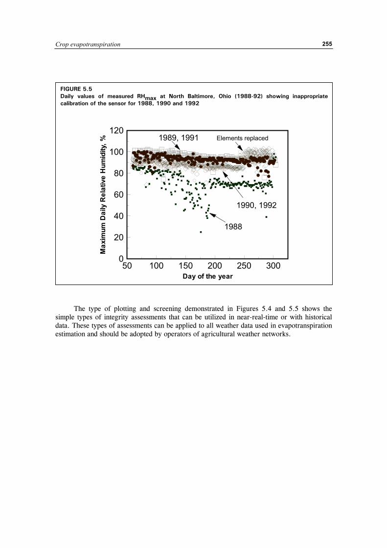
Crop evapotranspiration
255
The type of plotting and screening demonstrated in Figures 5.4 and 5.5 shows the simple types of integrity assessments that can be utilized in near-real-time or with historical data. These types of assessments can be applied to all weather data used in evapotranspiration estimation and should be adopted by operators of agricultural weather networks.
FIGURE 5.5 Daily values of measured RHmax at North Baltimore, Ohio (1988-92) showing inappropriate calibration of the sensor for 1988, 1990 and 1992
50 100 150 200 250 3000
20
40
60
80
100
120
Day of the year
Max
imum
Dai
ly R
elat
ive
Hum
idity
, %
1989, 1991
1990, 1992
1988
Elements replaced

Annex 5: Measuring and assessing integrity of weather data
256
Crop evapotranspiration
257
Annex 6
Correction of weather data observed in non-reference weather sites to compute ETo
The concept on which the FAO Penman – Monteith method for computing ETo is based requires that weather data be measured in environmental conditions that correspond to the definition of reference evapotranspiration. In other words, the weather data are to be measured above an extensive grass crop that is actively evapotranspiring, or in an environment with healthy vegetation not short of water1. Under these reference conditions, the energy available at the surface (Rn - G) is partitioned between sensible and latent heat (H and λE, respectively) in such a way that, in general, the ratio β = H/λEref ≤ 0.5. The subscript ref indicates reference conditions.
Environmental conditions of arid lands that surround a non reference (arid) weather site do not allow for the reference rate of evapotranspiration to be attained. This is generally caused by lack of well-watered conditions. Thus, λEn/ref < λEref (subscript n/ref for non reference conditions). If the available energy (Rn - G) is the same, then the partitioning among sensible and latent heat changes, with Hn/ref > Href and, often, βn/ref > 0.5. Consequently, since air temperature increases with increasing H, the air temperatures measured at non reference sites are higher than those that would have been measured if reference conditions had existed, i.e. Tn/ref > Tref. On the contrary, humidity measured at a non reference site is lower than that which would have occurred under reference conditions, thus ea n/ref < ea ref and VPDn/ref > VPDref.
When computing ETo using standard estimates for Rn - G, ra and rs, ETo will be overestimated when calculated using Tn/ref and VPDn/ref. A correction is therefore required to bring temperature and humidity data closer to the reference conditions.
In an environment having healthy vegetation and adequate soil moisture (reference conditions), minimum air temperature Tmin usually approaches dew point temperature, Tdew, (see Figure 6.2 for Kimberly, Idaho, the United States)2. This especially occurs if the wind dies down by early morning and when soil moisture is high (illustrated through the ratio precipitation/ETo, in Figure 6.1). Air temperatures decrease during night time due to surface cooling caused by long-wave emission and evaporation when VPD is positive. When near surface air temperature T approaches Tdew, T is prevented from decreasing below Tdew by condensation of vapour from the air and the correspondent heating effect of released latent heat. Thus, for reference conditions the relationship (Tmin)ref = (Tdew)ref is generally valid.
1 More detailed discussions are given in Allen (1996) and Allen et al (1996). 2 However, air temperature may not decrease to the dew point when large amounts of warm and dry
air are transported to the surface by wind.
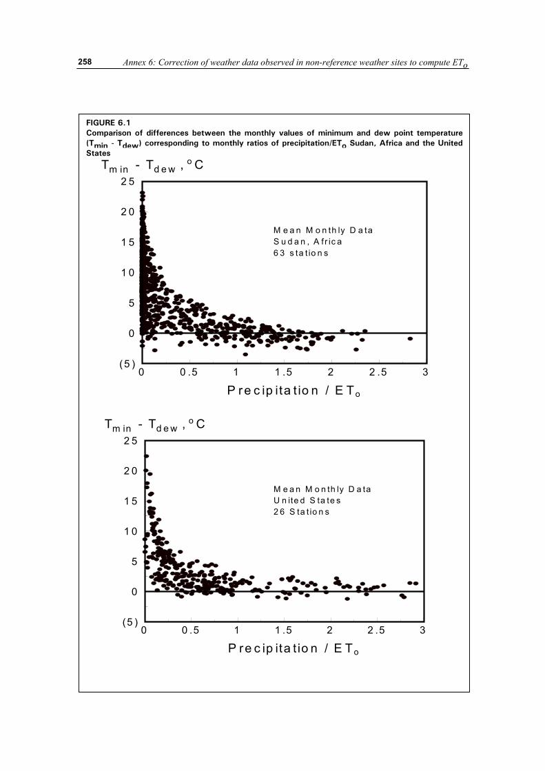
Annex 6: Correction of weather data observed in non-reference weather sites to compute ETo
258
FIGURE 6.1 Comparison of differences between the monthly values of minimum and dew point temperature (Tmin - Tdew) corresponding to monthly ratios of precipitation/ETo Sudan, Africa and the UnitedStates
0 0 .5 1 1 .5 2 2 .5 3(5 )
0
5
1 0
1 5
2 0
2 5
P re c ip ita t io n / E To
T - T , Cod e wm in
M e a n M o n th ly D a taS u d a n , A f r ic a6 3 s ta t io n s
0 0 .5 1 1 .5 2 2 .5 3(5 )
0
5
1 0
1 5
2 0
2 5
P re c ip ita t io n / E To
T - T , Cod e wm in
M e a n M o n th ly D a taU n ite d S ta te s2 6 S ta t io n s
Crop evapotranspiration
259
For non reference sites, soil moisture and/or vegetation limitations make λETn/ref < λETref or ETn/ref < ETo. Thus Tmin may remain above Tdew. One cause of this phenomenon is the large "reservoir" of sensible heat created during daytime in the atmosphere (Hn/ref > Href, as suggested before), which is transferred towards the surface during the night, reducing the effect of cooling by long wave radiation. Another cause is the lack of soil moisture for evaporative cooling during night time.
This phenomenon can be observed in Figure 6.1, where monthly means for Tmin - Tdew
are plotted for weather stations operated by national governments of two countries, Sudan and the United States. The data are plotted against the monthly ratios of precipitation to reference ETo. The P/ETo ratios indicate the availability of adequate soil water to support reference (well-watered) conditions in the absense of irrigation. As illustrated by the data, Tmin approaches Tdew for nearly all stations when the ratio P/ETo approaches and exceeds 1. When P/ETo < 1, then the aridity of the station causes Tmin to substantially exceed measured Tdew. The exception is for those weather stations that have P/ETo < 1, but are irrigated or have adequate soil water reserves from a prior month. The similarity between data of Sudan and the United States indicates that this is a general phenomenon.
An additional comparison is given in Figure 2, where Tmin - Tdew are compared for two semiarid locations in Idaho, the United States that are separated by 200 km. One location, Kimberly, is a reference site in the middle of a large irrigated area. The other, Boise, is a non reference site, located at an airport and surrounded by a mixture of irrigated and non irrigated rangeland. It can be seen that Tmin approaches Tdew frequently for the irrigated site at Kimberly, with only small differences occuring during months where a dry climate occurs (low precipitation/ETo ratio). On the contrary, Tmin was as much as 10ºC higher than Tdew for the nonreference Boise station. From this graphical comparison, one can conclude that data for the nonreference Boise site require appropriate correction before being utilized to compute ETo using the FAO - PM method. This is necessary to avoid overestimation of ETo due to overestimation of air temperature and VPD.
Adjustment of Tmax, Tmin and Tdew
The empirical method described herein intends to correct the observed temperatures, Tmax and Tmin in proportion to the difference (Tmin - Tdew), which works as an indicator of the overestimation of (Tn/ref - Tref). Since Tdew defines the actual vapour pressure (ea = eº (Tdew)), correcting Tdew also provides an adjustment for VPD. The methodology proposed is the following: 1. Compare Tmin - Tdew (Tdew measured or computed from ea using equations (11) or
(12) in Annex 3) from a non reference site with those from a reference site using a graphical procedure such as in Figure 6.2 and using monthly ratios of Precipitation/ETo as the abcissa. Daily or monthly data are utilized to compute Tmin - Tdew.
2. When differences Tmin - Tdew for the non reference site are systematically higher than about 2ºC relative to the reference site, then compute the average differences
∆T = T - Tmin dew (6-1)
for the months which require correction (in general this will occur when the monthly ratio Precipitation/ETo does not exceed 0.5).
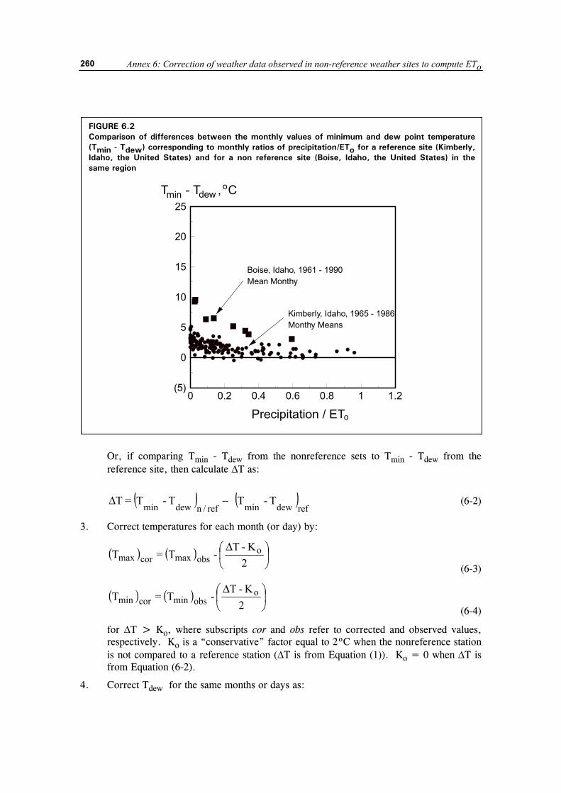
Annex 6: Correction of weather data observed in non-reference weather sites to compute ETo
260
Or, if comparing Tmin - Tdew from the nonreference sets to Tmin - Tdew from the reference site, then calculate ∆T as:
( ) ( )refdewminref/ndewmin T - T T - T = T −∆ (6-2)
3. Correct temperatures for each month (or day) by:
( ) ( ) ��
���
� ∆2
K -T - T = T o
obsmaxcormax (6-3)
( ) ( ) ��
���
� ∆2
K -T - T = T o
obsmincormin (6-4)
for ∆T > Ko, where subscripts cor and obs refer to corrected and observed values, respectively. Ko is a “conservative” factor equal to 2ºC when the nonreference station is not compared to a reference station (∆T is from Equation (1)). Ko = 0 when ∆T is from Equation (6-2).
4. Correct Tdew for the same months or days as:
FIGURE 6.2 Comparison of differences between the monthly values of minimum and dew point temperature (Tmin - Tdew) corresponding to monthly ratios of precipitation/ETo for a reference site (Kimberly, Idaho, the United States) and for a non reference site (Boise, Idaho, the United States) in the same region
0 0.2 0.4 0.6 0.8 1 1.2(5)
0
5
10
15
20
25
Precipitation / ETo
T - T , Codewmin
Boise, Idaho, 1961 - 1990Mean Monthy
Kimberly, Idaho, 1965 - 1986Monthy Means
Crop evapotranspiration
261
( ) ( ) ��
���
� ∆2
K-T + T = T o
obsdewcordew (6-5)
where Ko has the same value as for Equations (6-3) and (6-4), and utilizing either the observed or the calculated values for Tdew (equations (3-11) or (3-12) in Annex 3). The user should always insure that (Tmin)cor ≥ (Tdew)cor.
5. Compute ETo with the corrected values for Tmax, Tmin and Tdew. Adjustment of Tdew only
When RH, ea, or Tdew data are not dependable or where “correction” of Tmax and Tmin as is done in the previous section is undesireable, a second means for “correcting” the weather data set for station aridity is possible. This second method is to merely set
omindew KTT −= (6-6)
in the calculation for ETo where Ko = 0ºC for humid and subhumid climates and Ko = 2ºC for arid and semiarid climates. The result of this procedure is to increase Tdew to reflect the higher humidity anticipated under reference conditions. It is noted that in a nonreference setting, the measured Tmin may be too high, as compared to Tmin expected for a reference setting, so that Equation (6-6) may result in values for Tdew that are overestimated, even for a reference condition. However, since the computation of vapor pressure deficit, VPD, in the ETo equation, where VPD = 0.5(eo(Tmax) + eo(Tmin)) - eo(Tdew), utilizes values for air temperature and dew point temperature that may both be too high, the upward bias in all temperature parameters will tend to cancel, thereby presenting a VPD that is representative of a reference condition. Index for station aridity
For non reference sites, when humidity data are available, one can compute an aridity bias index Abi (for monthly time scales)
( )( )AETbi
obs
o T dew
= ET
- 1
o
= T min
(6-7)
between the ETo computed from the observed (non-corrected) data (subscript obs) and, for the same period, using Tmin as an estimate of Tdew. If there is not a large difference between Tmin and Tdew, then Abi~0. When ∆T = Tmin - Tdew is large (i.e., for a nonreference condition), then the aridity bias index Abi becomes > 0.
The user should compare aridity bias indices for the dry and humid months and decide whether higher values for Abi result from aridity or from other causes. A correction may be required when Abi are consistently greater than 0.05. The correction of temperature and humidity data can be performed as indicated in the previous sections.
It is important for the user to realize that these corrections are to improve the calculations of ETo only, since ETo is defined for a well-watered environment. For hydrology studies where actual ET is required, then no adjustment should be made to air temperature and dew point temperature, since the ETo n/ref characterises the natural evaporation demands of the climate.

Annex 6: Correction of weather data observed in non-reference weather sites to compute ETo
262
Any corrected Tmax, Tmin, Tdew data should not be reintroduced into the original historical data series. Also, the user should note that all of the correction procedures presented here are only approximate attempts to bring the ETo calculations closer to the “real” ETo that reflects a well-watered environment. Any errors or uncertainties introduced by these adjustments at a specific site will remain largely unknown. Therefore the user is encouraged to use caution.
Crop evapotranspiration
263
Annex 7
Background and computations for Kc for the initial stage for annual crops
ET during the initial stage for annual crops is predominately in the form of evaporation. Therefore, accurate estimates for Kc ini must consider the frequency that the soil surface is wetted during the initial period. The initial period was defined in Chapter 6 for annual crops as the period between the planting date and the date of approximately 10% ground cover. Chapter 6 presents background and figures for predicting Kc ini as a function of reference evapotranspiration (ETo), soil texture, and frequency and depth of wetting. Additional background and equations are given in Chapter 7. This annex provides further background on development of the Kc ini curves that are presented in Figures 29 and 30 of Chapter 6. Equations are presented here that can be used in place of Figures 29 and 30 when computers are used. INTRODUCTION Evaporation from bare soil (Es) can be characterized as occurring in two distinct stages. The stage 1 is termed the "energy limited" stage. During this stage, moisture is transported to the soil surface at a rate sufficient to supply the potential rate of evaporation (Eso), which, in turn, is governed by energy availability at the soil surface. In this procedure, Eso is estimated from
oso ET15.1E = (7-1)
where Eso is the potential rate of evaporation [mm d-1] and ETo is the the mean ETo during the initial period [mm d-1]. The value 1.15 represents increased evaporation potential due to low albedo of wet soil and the possibility of heat stored in the surface layer during previous dry periods. Stage 2 is termed the "soil limited" stage, where hydraulic transport of subsurface water to the soil surface is unable to supply water at the potential evaporation rate. During stage 2, the soil surface appears partially dry and a portion of the evaporation occurs from below the soil surface. The energy required for subsurface evaporation is supplied by transport of heat from the soil surface into the soil profile. The evaporation rate during stage 2 drying decreases as soil water content decreases as shown in Figure 7.1 (see also Figure 38 of Chapter 7). The evaporation rate can therefore be expressed as being proportional to the water remaining in the evaporation layer relative to the maximum depth of water that can be evaporated from the same soil layer during stage 2 drying.
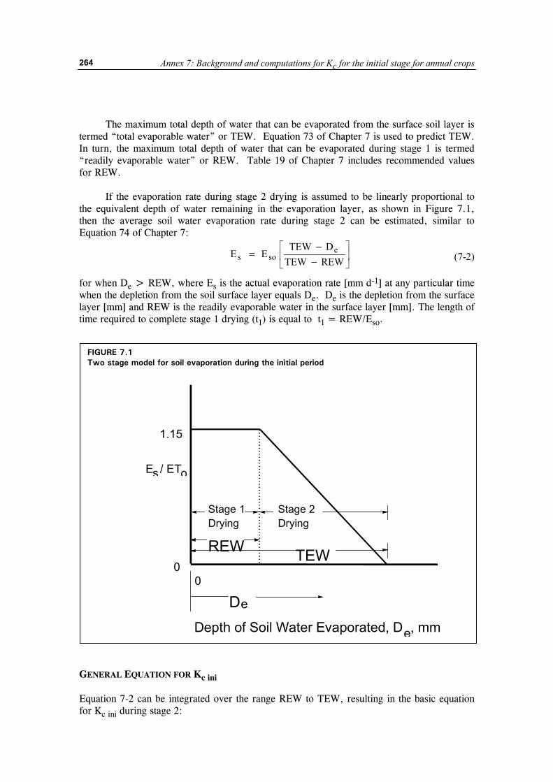
Annex 7: Background and computations for Kc for the initial stage for annual crops
264
The maximum total depth of water that can be evaporated from the surface soil layer is termed “total evaporable water” or TEW. Equation 73 of Chapter 7 is used to predict TEW. In turn, the maximum total depth of water that can be evaporated during stage 1 is termed “readily evaporable water” or REW. Table 19 of Chapter 7 includes recommended values for REW. If the evaporation rate during stage 2 drying is assumed to be linearly proportional to the equivalent depth of water remaining in the evaporation layer, as shown in Figure 7.1, then the average soil water evaporation rate during stage 2 can be estimated, similar to Equation 74 of Chapter 7:
��
���
�
−−
=REWTEWDTEW
EE esos (7-2)
for when De > REW, where Es is the actual evaporation rate [mm d-1] at any particular time when the depletion from the soil surface layer equals De. De is the depletion from the surface layer [mm] and REW is the readily evaporable water in the surface layer [mm]. The length of time required to complete stage 1 drying (t1) is equal to t1 = REW/Eso.
GENERAL EQUATION FOR Kc ini Equation 7-2 can be integrated over the range REW to TEW, resulting in the basic equation for Kc ini during stage 2:
FIGURE 7.1 Two stage model for soil evaporation during the initial period
E / ETs
Depth of Soil Water Evaporated, D , mme
Stage 1Drying
Stage 2Drying
REW TEW
De
o
1.15
00
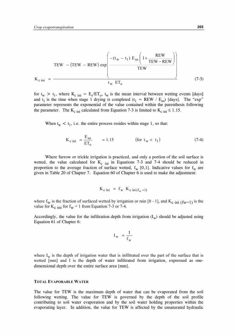
Crop evapotranspiration
265
( )
ow
so1w
inic ETt
TEWREWTEW
REW1E)tt(expREWTEWTEW
K�����
�
�
�����
�
����
����
�
−+−−
−−
= (7-3)
for tw > t1, where Kc ini = Es/ETo, tw is the mean interval between wetting events [days] and t1 is the time when stage 1 drying is completed (t1 = REW / Eso) [days]. The “exp” parameter represents the exponential of the value contained within the parenthesis following the parameter. The Kc ini calculated from Equation 7-3 is limited to Kc ini ≤ 1.15.
When tw < t1, i.e. the entire process resides within stage 1, so that:
( )1wo
soinic ttfor15.1
ETE
K <== (7-4)
Where furrow or trickle irrigation is practiced, and only a portion of the soil surface is wetted, the value calculated for Kc ini in Equations 7-3 and 7-4 should be reduced in proportion to the average fraction of surface wetted, fw [0,1]. Indicative values for fw are given in Table 20 of Chapter 7. Equation 60 of Chapter 6 is used to make the adjustment: )1f(inicwinic w
KfK ==
where fw is the fraction of surfaced wetted by irrigation or rain [0 - 1], and Kc ini (fw=1) is the value for Kc ini for fw = 1 from Equation 7-3 or 7-4. Accordingly, the value for the infiltration depth from irrigation (Iw) should be adjusted using Equation 61 of Chapter 6:
w
w fII =
where Iw is the depth of irrigation water that is infiltrated over the part of the surface that is wetted [mm] and I is the depth of water infiltrated from irrigation, expressed as one-dimensional depth over the entire surface area [mm]. TOTAL EVAPORABLE WATER The value for TEW is the maximum depth of water that can be evaporated from the soil following wetting. The value for TEW is governed by the depth of the soil profile contributing to soil water evaporation and by the soil water holding properties within the evaporating layer. In addition, the value for TEW is affected by the unsaturated hydraulic
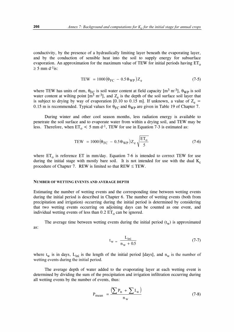
Annex 7: Background and computations for Kc for the initial stage for annual crops
266
conductivity, by the presence of a hydraulically limiting layer beneath the evaporating layer, and by the conduction of sensible heat into the soil to supply energy for subsurface evaporation. An approximation for the maximum value of TEW for initial periods having ETo ≥ 5 mm d-1is:
( ) eWPFC Z5.01000TEW θ−θ= (7-5)
where TEW has units of mm, θFC is soil water content at field capacity [m3 m-3], θWP is soil water content at wilting point [m3 m-3], and Ze is the depth of the soil surface soil layer that is subject to drying by way of evaporation [0.10 to 0.15 m]. If unknown, a value of Ze = 0.15 m is recommended. Typical values for θFC and θWP are given in Table 19 of Chapter 7. During winter and other cool season months, less radiation energy is available to penetrate the soil surface and to evaporate water from within a drying soil, and TEW may be less. Therefore, when ETo < 5 mm d-1, TEW for use in Equation 7-3 is estimated as:
( )5
ETZ5.01000TEW o
eWPFC θ−θ= (7-6)
where ETo is reference ET in mm/day. Equation 7-6 is intended to correct TEW for use during the initial stage with mostly bare soil. It is not intended for use with the dual Kc procedure of Chapter 7. REW is limited so that REW ≤ TEW. NUMBER OF WETTING EVENTS AND AVERAGE DEPTH Estimating the number of wetting events and the corresponding time between wetting events during the initial period is described in Chapter 6. The number of wetting events (both from precipitation and irrigation) occurring during the initial period is determined by considering that two wetting events occurring on adjoining days can be counted as one event, and individual wetting events of less than 0.2 ETo can be ignored.
The average time between wetting events during the initial period (tw) is approximated as:
t Lnw
ini
w= + 0 5.
(7-7)
where tw is in days, Lini is the length of the initial period [days], and nw is the number of wetting events during the initial period.
The average depth of water added to the evaporating layer at each wetting event is determined by dividing the sum of the precipitation and irrigation infiltration occurring during all wetting events by the number of events, thus:
( )
w
wnmean n
IPP � �+
= (7-8)
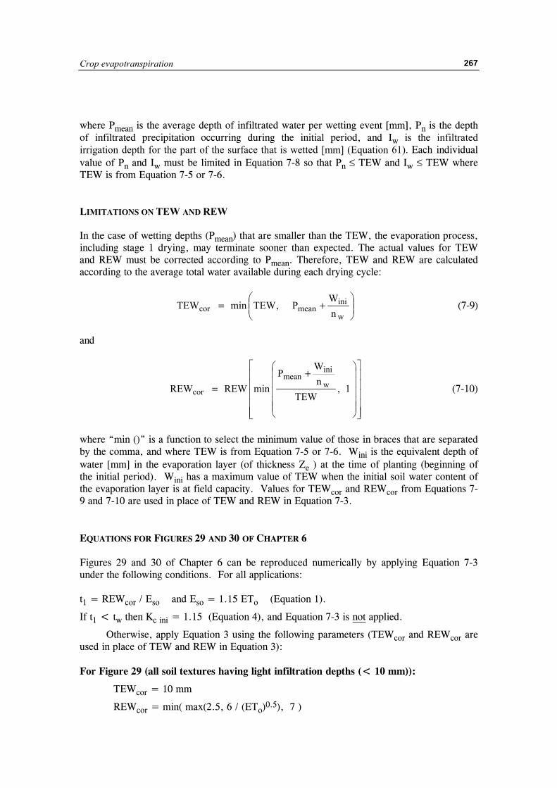
Crop evapotranspiration
267
where Pmean is the average depth of infiltrated water per wetting event [mm], Pn is the depth of infiltrated precipitation occurring during the initial period, and Iw is the infiltrated irrigation depth for the part of the surface that is wetted [mm] (Equation 61). Each individual value of Pn and Iw must be limited in Equation 7-8 so that Pn ≤ TEW and Iw ≤ TEW where TEW is from Equation 7-5 or 7-6. LIMITATIONS ON TEW AND REW In the case of wetting depths (Pmean) that are smaller than the TEW, the evaporation process, including stage 1 drying, may terminate sooner than expected. The actual values for TEW and REW must be corrected according to Pmean. Therefore, TEW and REW are calculated according to the average total water available during each drying cycle:
���
����
�+=
w
inimeancor n
WP,TEWminTEW (7-9)
and
�����
�
�
�����
�
�
�����
�
�
� += 1,
TEWn
WP
minREWREW w
inimean
cor (7-10)
where “min ()” is a function to select the minimum value of those in braces that are separated by the comma, and where TEW is from Equation 7-5 or 7-6. Wini is the equivalent depth of water [mm] in the evaporation layer (of thickness Ze ) at the time of planting (beginning of the initial period). Wini has a maximum value of TEW when the initial soil water content of the evaporation layer is at field capacity. Values for TEWcor and REWcor from Equations 7-9 and 7-10 are used in place of TEW and REW in Equation 7-3. EQUATIONS FOR FIGURES 29 AND 30 OF CHAPTER 6 Figures 29 and 30 of Chapter 6 can be reproduced numerically by applying Equation 7-3 under the following conditions. For all applications: t1 = REWcor / Eso and Eso = 1.15 ETo (Equation 1).
If t1 < tw then Kc ini = 1.15 (Equation 4), and Equation 7-3 is not applied.
Otherwise, apply Equation 3 using the following parameters (TEWcor and REWcor are used in place of TEW and REW in Equation 3): For Figure 29 (all soil textures having light infiltration depths (< 10 mm)):
TEWcor = 10 mm
REWcor = min( max(2.5, 6 / (ETo)0.5), 7 )
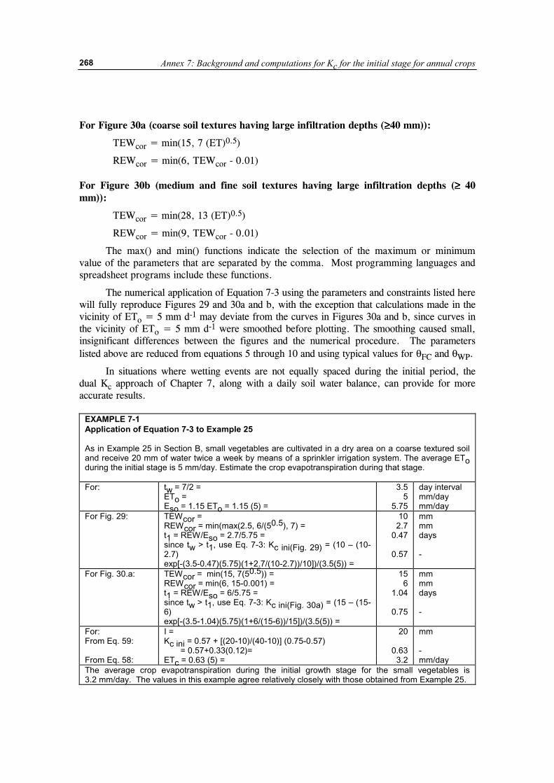
Annex 7: Background and computations for Kc for the initial stage for annual crops
268
For Figure 30a (coarse soil textures having large infiltration depths (≥≥≥≥40 mm)):
TEWcor = min(15, 7 (ET)0.5)
REWcor = min(6, TEWcor - 0.01) For Figure 30b (medium and fine soil textures having large infiltration depths (≥≥≥≥ 40 mm)):
TEWcor = min(28, 13 (ET)0.5)
REWcor = min(9, TEWcor - 0.01)
The max() and min() functions indicate the selection of the maximum or minimum value of the parameters that are separated by the comma. Most programming languages and spreadsheet programs include these functions.
The numerical application of Equation 7-3 using the parameters and constraints listed here will fully reproduce Figures 29 and 30a and b, with the exception that calculations made in the vicinity of ETo = 5 mm d-1 may deviate from the curves in Figures 30a and b, since curves in the vicinity of ETo = 5 mm d-1 were smoothed before plotting. The smoothing caused small, insignificant differences between the figures and the numerical procedure. The parameters listed above are reduced from equations 5 through 10 and using typical values for θFC and θWP.
In situations where wetting events are not equally spaced during the initial period, the dual Kc approach of Chapter 7, along with a daily soil water balance, can provide for more accurate results.
EXAMPLE 7-1 Application of Equation 7-3 to Example 25 As in Example 25 in Section B, small vegetables are cultivated in a dry area on a coarse textured soil and receive 20 mm of water twice a week by means of a sprinkler irrigation system. The average ETo during the initial stage is 5 mm/day. Estimate the crop evapotranspiration during that stage. For:
tw = 7/2 = ETo = Eso = 1.15 ETo = 1.15 (5) =
3.5 5
5.75
day interval mm/day mm/day
For Fig. 29:
TEWcor = REWcor = min(max(2.5, 6/(50.5), 7) = t1 = REW/Eso = 2.7/5.75 = since tw > t1, use Eq. 7-3: Kc ini(Fig. 29) = (10 – (10-2.7) exp[-(3.5-0.47)(5.75)(1+2.7/(10-2.7))/10])/(3.5(5)) =
10 2.7
0.47
0.57
mm mm days -
For Fig. 30.a:
TEWcor = min(15, 7(50.5)) = REWcor = min(6, 15-0.001) = t1 = REW/Eso = 6/5.75 = since tw > t1, use Eq. 7-3: Kc ini(Fig. 30a) = (15 – (15-6) exp[-(3.5-1.04)(5.75)(1+6/(15-6))/15])/(3.5(5)) =
15 6
1.04
0.75
mm mm days -
For: I = 20 mm From Eq. 59:
Kc ini = 0.57 + [(20-10)/(40-10)] (0.75-0.57) = 0.57+0.33(0.12)=
0.63
-
From Eq. 58: ETc = 0.63 (5) = 3.2 mm/day The average crop evapotranspiration during the initial growth stage for the small vegetables is 3.2 mm/day. The values in this example agree relatively closely with those obtained from Example 25.
Crop evapotranspiration
269
Annex 8
Calculation example for applying the dual Kc procedure in irrigation scheduling
This annex illustrates in more detail the application of the various equations for calculating Kcb, Ke and ETc using the dual Kc approach of Chapter 7. The example is in the form of a computer spreadsheet and is applied to the dry, edible bean crop that was used in example boxes 15 and 16 of Chapters 6 and 7. The spreadsheet is shown in Figure 8.1, where the irrigation schedule is determined using the daily soil-water balance procedure described in Chapter 8. The timing of irrigations is based on the management allowed depletion (MAD) of the available water that can be stored in the root zone. The irrigation schedule and the corresponding estimated wet soil evaporation are different from the actual values shown in Box 16 of Chapter 7, since Box 16 represents the actual irrigation schedule used at Kimberly during 1974. The actual schedule deviated somewhat from the theoretical schedule of Figure 8.1. The spreadsheet formulas used for calculations and the references to equations in the text are indicated in Box 8.1. The variable names used for parameters follow the same convention used in Chapters 1 to 9. The variable names are defined in the List of principal symbols and acronymns in the introduction to this paper. A few exceptions are defined in Table 8.1.
The spreadsheet in Figure 8.1 includes columns for variables Tmax, u2, and Tdew. The Tmax and Tdew columns are used to calculate daily RHmin. The u2 and RHmin columns are used to adjust Kcb mid and Kcb end using Equation 70 of Chapter 7 and to calculate Kc max using Equation 72 on a daily basis. The data in the first 7 rows of Figure 8.1 that appear within boxes represent the specific crop and soils information that is entered by the user for a particular crop and soil combination. All other information (outside of boxes) is calculated automatically by the spreadsheet program. The columns having double underlined headings represent the data that are input by the user into the spreadsheet. The calculations in Figure 8.1 can be used to verify other computer programs or spreadsheet calculations for Ke, Kc and ETc. Small differences may result, depending on the assumptions of timing of irrigations. The spreadsheet of Figure 8.1 presumes that all irrigation and precipitation events occur early in the morning. The scheduling and magnitudes of irrigations are based on the soil water depletion at the end of the previous day. The spreadsheet also presumes that all drainage from the root zone due to excess precipitation occurs on the day of the precipitation event. It is assumed that runoff from precipitation is zero. If necessary, procedures for predicting precipitation runoff can be entered into the spreadsheet using procedures described in most standard hydrology textbooks. It is assumed that the net depth of irrigation that is retained in the crop root zone is exactly equal to the depletion depth of the previous day. This assumption presumes perfect knowledge of soil water depletion by the irrigator or that all irrigations are adequate or excessive. This assumption may not hold for some irrigation conditions and can be changed by the user as needed.

Annex 8:Calculation example for applying the dual Kc procedure in irrigation scheduling
270
Spreadsheet formulas used to create the spreadsheet of Figure 8.1 are listed in Box 8.1 for the Microsoft Excel language (versions 5 and higher). Formulae for other types of spreadsheets would be similar. Formulae for the Corel Quattro-Pro language (versions 5 and higher) can be downloaded from the FAO internet site.

Crop evapotranspiration
271

Annex 8:Calculation example for applying the dual Kc procedure in irrigation scheduling
272

Crop evapotranspiration
273
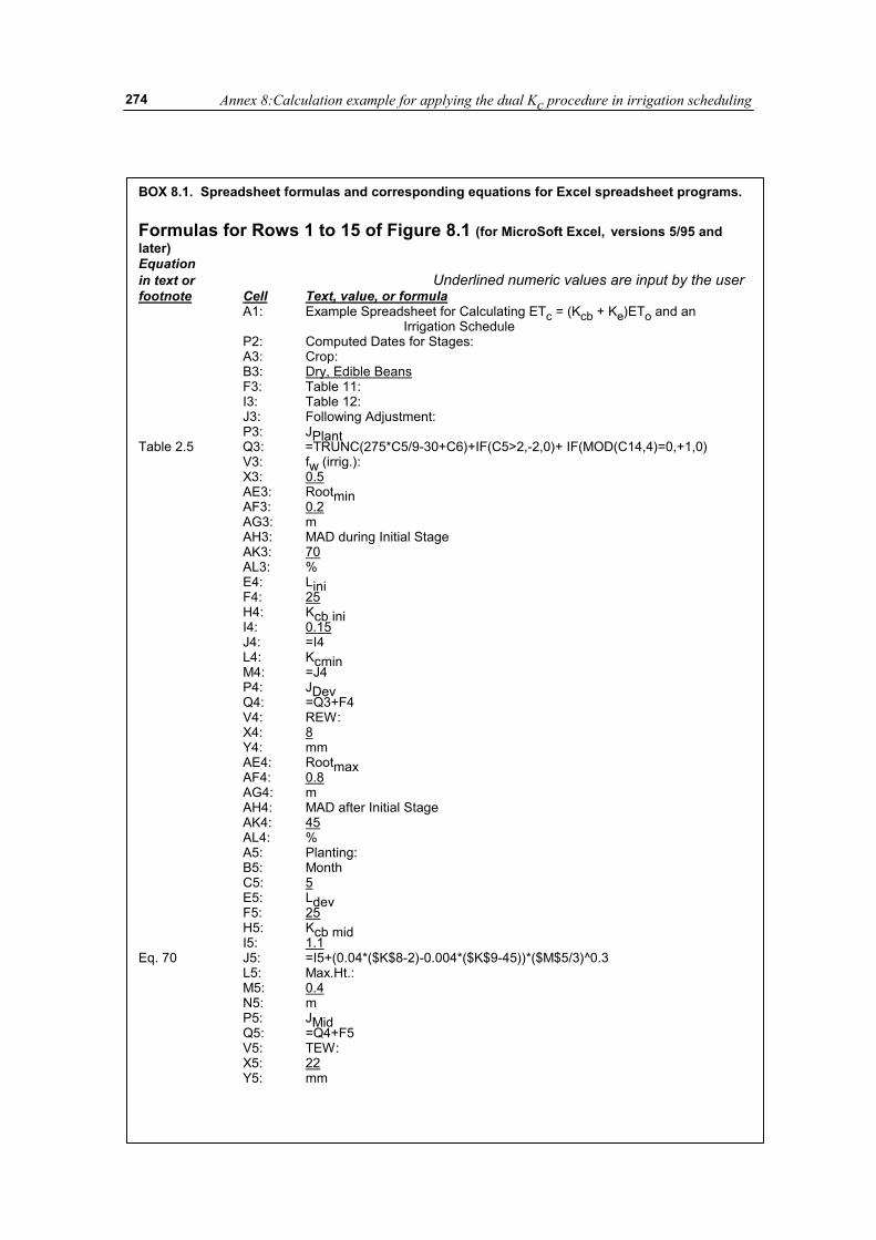
Annex 8:Calculation example for applying the dual Kc procedure in irrigation scheduling
274
BOX 8.1. Spreadsheet formulas and corresponding equations for Excel spreadsheet programs. Formulas for Rows 1 to 15 of Figure 8.1 (for MicroSoft Excel, versions 5/95 and later) Equation in text or Underlined numeric values are input by the user footnote Cell Text, value, or formula A1: Example Spreadsheet for Calculating ETc = (Kcb + Ke)ETo and an Irrigation Schedule P2: Computed Dates for Stages: A3: Crop: B3: Dry, Edible Beans F3: Table 11: I3: Table 12: J3: Following Adjustment: P3: JPlant Table 2.5 Q3: =TRUNC(275*C5/9-30+C6)+IF(C5>2,-2,0)+ IF(MOD(C14,4)=0,+1,0) V3: fw (irrig.): X3: 0.5 AE3: Rootmin AF3: 0.2 AG3: m AH3: MAD during Initial Stage AK3: 70 AL3: % E4: Lini F4: 25 H4: Kcb ini I4: 0.15 J4: =I4 L4: Kcmin M4: =J4 P4: JDev Q4: =Q3+F4 V4: REW: X4: 8 Y4: mm AE4: Rootmax AF4: 0.8 AG4: m AH4: MAD after Initial Stage AK4: 45 AL4: % A5: Planting: B5: Month C5: 5 E5: Ldev F5: 25 H5: Kcb mid I5: 1.1 Eq. 70 J5: =I5+(0.04*($K$8-2)-0.004*($K$9-45))*($M$5/3)^0.3 L5: Max.Ht.: M5: 0.4 N5: m P5: JMid Q5: =Q4+F5 V5: TEW: X5: 22 Y5: mm
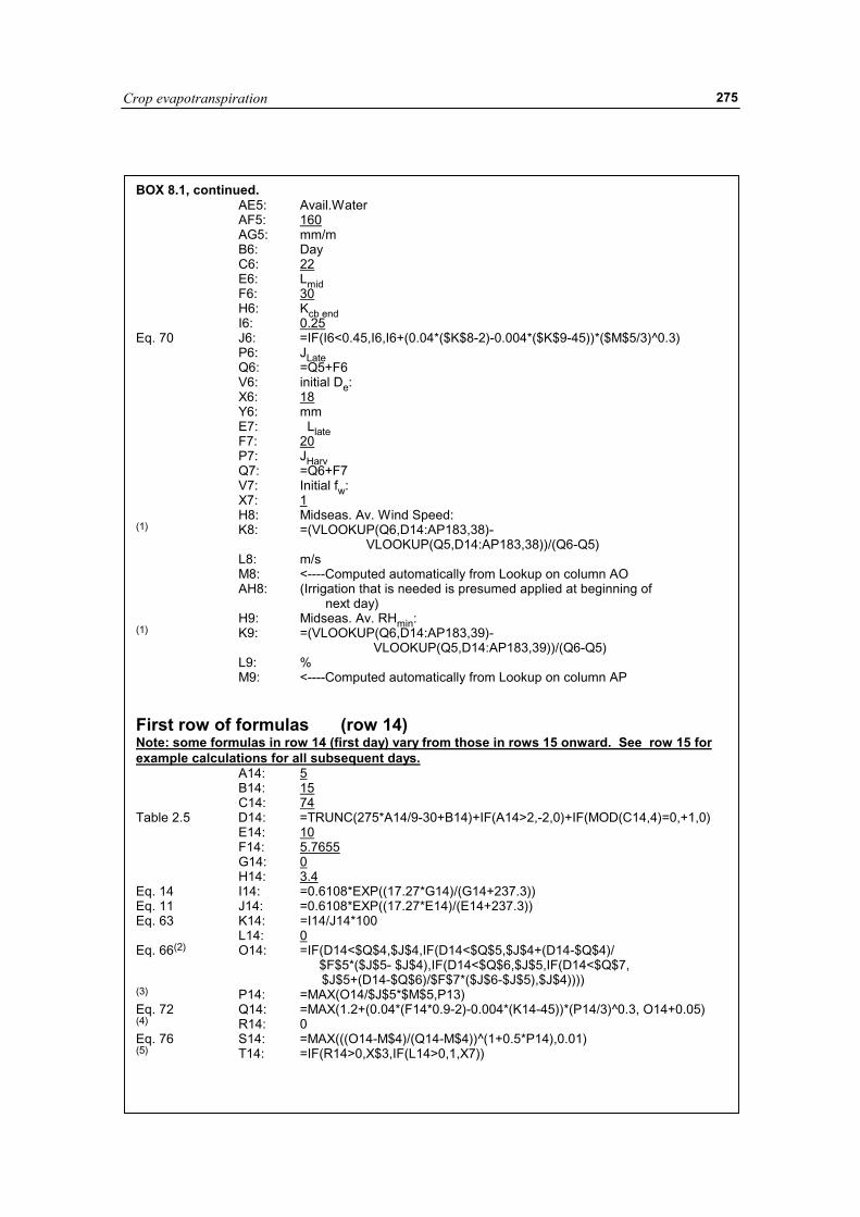
Crop evapotranspiration
275
BOX 8.1, continued. AE5: Avail.Water AF5: 160 AG5: mm/m B6: Day C6: 22 E6: Lmid F6: 30 H6: Kcb end I6: 0.25 Eq. 70 J6: =IF(I6<0.45,I6,I6+(0.04*($K$8-2)-0.004*($K$9-45))*($M$5/3)^0.3) P6: JLate Q6: =Q5+F6 V6: initial De: X6: 18 Y6: mm E7: Llate F7: 20 P7: JHarv Q7: =Q6+F7 V7: Initial fw: X7: 1 H8: Midseas. Av. Wind Speed: (1) K8: =(VLOOKUP(Q6,D14:AP183,38)- VLOOKUP(Q5,D14:AP183,38))/(Q6-Q5) L8: m/s M8: <----Computed automatically from Lookup on column AO AH8: (Irrigation that is needed is presumed applied at beginning of next day) H9: Midseas. Av. RHmin: (1) K9: =(VLOOKUP(Q6,D14:AP183,39)- VLOOKUP(Q5,D14:AP183,39))/(Q6-Q5) L9: % M9: <----Computed automatically from Lookup on column AP First row of formulas (row 14) Note: some formulas in row 14 (first day) vary from those in rows 15 onward. See row 15 for example calculations for all subsequent days. A14: 5 B14: 15 C14: 74 Table 2.5 D14: =TRUNC(275*A14/9-30+B14)+IF(A14>2,-2,0)+IF(MOD(C14,4)=0,+1,0) E14: 10 F14: 5.7655 G14: 0 H14: 3.4 Eq. 14 I14: =0.6108*EXP((17.27*G14)/(G14+237.3)) Eq. 11 J14: =0.6108*EXP((17.27*E14)/(E14+237.3)) Eq. 63 K14: =I14/J14*100 L14: 0 Eq. 66(2) O14: =IF(D14<$Q$4,$J$4,IF(D14<$Q$5,$J$4+(D14-$Q$4)/ $F$5*($J$5- $J$4),IF(D14<$Q$6,$J$5,IF(D14<$Q$7, $J$5+(D14-$Q$6)/$F$7*($J$6-$J$5),$J$4)))) (3) P14: =MAX(O14/$J$5*$M$5,P13) Eq. 72 Q14: =MAX(1.2+(0.04*(F14*0.9-2)-0.004*(K14-45))*(P14/3)^0.3, O14+0.05) (4) R14: 0 Eq. 76 S14: =MAX(((O14-M$4)/(Q14-M$4))^(1+0.5*P14),0.01) (5) T14: =IF(R14>0,X$3,IF(L14>0,1,X7))
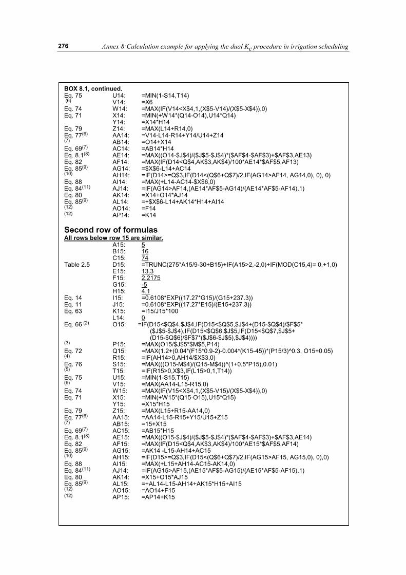
Annex 8:Calculation example for applying the dual Kc procedure in irrigation scheduling
276
BOX 8.1, continued. Eq. 75 U14: =MIN(1-S14,T14) (6) V14: =X6 Eq. 74 W14: =MAX(IF(V14<X$4,1,(X$5-V14)/(X$5-X$4)),0) Eq. 71 X14: =MIN(+W14*(Q14-O14),U14*Q14) Y14: =X14*H14 Eq. 79 Z14: =MAX(L14+R14,0) Eq. 77(6) AA14: =V14-L14-R14+Y14/U14+Z14 (7) AB14: =O14+X14 Eq. 69(7) AC14: =AB14*H14 Eq. 8.1(8) AE14: =MAX((O14-$J$4)/($J$5-$J$4)*($AF$4-$AF$3)+$AF$3,AE13) Eq. 82 AF14: =MAX(IF(D14<Q$4,AK$3,AK$4)/100*AE14*$AF$5,AF13) Eq. 85(9) AG14: =$X$6-L14+AC14 (10) AH14: =IF(D14>=Q$3,IF(D14<(Q$6+Q$7)/2,IF(AG14>AF14, AG14,0), 0), 0) Eq. 88 AI14: =MAX(+L14-AC14-$X$6,0) Eq. 84(11) AJ14: =IF(AG14>AF14,(AE14*AF$5-AG14)/(AE14*AF$5-AF14),1) Eq. 80 AK14: =X14+O14*AJ14 Eq. 85(9) AL14: =+$X$6-L14+AK14*H14+AI14 (12) AO14: =F14 (12) AP14: =K14 Second row of formulas All rows below row 15 are similar. A15: 5 B15: 16 C15: 74 Table 2.5 D15: =TRUNC(275*A15/9-30+B15)+IF(A15>2,-2,0)+IF(MOD(C15,4)= 0,+1,0) E15: 13.3 F15: 2.2175 G15: -5 H15: 4.1 Eq. 14 I15: =0.6108*EXP((17.27*G15)/(G15+237.3)) Eq. 11 J15: =0.6108*EXP((17.27*E15)/(E15+237.3)) Eq. 63 K15: =I15/J15*100 L14: 0 Eq. 66 (2) O15: =IF(D15<$Q$4,$J$4,IF(D15<$Q$5,$J$4+(D15-$Q$4)/$F$5* ($J$5-$J$4),IF(D15<$Q$6,$J$5,IF(D15<$Q$7,$J$5+ (D15-$Q$6)/$F$7*($J$6-$J$5),$J$4)))) (3) P15: =MAX(O15/$J$5*$M$5,P14) Eq. 72 Q15: =MAX(1.2+(0.04*(F15*0.9-2)-0.004*(K15-45))*(P15/3)^0.3, O15+0.05) (4) R15: =IF(AH14>0,AH14/$X$3,0) Eq. 76 S15: =MAX(((O15-M$4)/(Q15-M$4))^(1+0.5*P15),0.01) (5) T15: =IF(R15>0,X$3,IF(L15>0,1,T14)) Eq. 75 U15: =MIN(1-S15,T15) (6) V15: =MAX(AA14-L15-R15,0) Eq. 74 W15: =MAX(IF(V15<X$4,1,(X$5-V15)/(X$5-X$4)),0) Eq. 71 X15: =MIN(+W15*(Q15-O15),U15*Q15) Y15: =X15*H15 Eq. 79 Z15: =MAX(L15+R15-AA14,0) Eq. 77(6) AA15: =AA14-L15-R15+Y15/U15+Z15 (7) AB15: =15+X15 Eq. 69(7) AC15: =AB15*H15 Eq. 8.1(8) AE15: =MAX((O15-$J$4)/($J$5-$J$4)*($AF$4-$AF$3)+$AF$3,AE14) Eq. 82 AF15: =MAX(IF(D15<Q$4,AK$3,AK$4)/100*AE15*$AF$5,AF14) Eq. 85(9) AG15: =AK14 -L15-AH14+AC15 (10) AH15: =IF(D15>=Q$3,IF(D15<(Q$6+Q$7)/2,IF(AG15>AF15, AG15,0), 0),0) Eq. 88 AI15: =MAX(+L15+AH14-AC15-AK14,0) Eq. 84(11) AJ14: =IF(AG15>AF15,(AE15*AF$5-AG15)/(AE15*AF$5-AF15),1) Eq. 80 AK14: =X15+O15*AJ15 Eq. 85(9) AL15: =+AL14-L15-AH14+AK15*H15+AI15 (12) AO15: =AO14+F15 (12) AP15: =AP14+K15
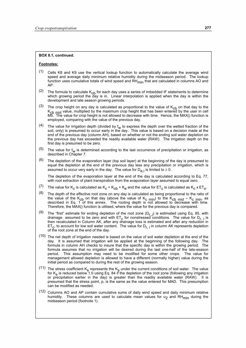
Crop evapotranspiration
277
BOX 8.1, continued. Footnotes: (1) Cells K8 and K9 use the vertical lookup function to automatically calculate the average wind
speed and average daily minimum relative humidity during the midseason period. The lookup function uses cumulative totals of wind speed and RHmin that are calculated in columns AO and AP.
(2) The formula to calculate Kcb for each day uses a series of imbedded IF statements to determine which growing period the day is in. Linear interpolation is applied when the day is within the development and late season growing periods.
(3) The crop height on any day is calculated as proportional to the value of Kcb on that day to the Kcb mid value, multiplied by the maximum crop height that has been entered by the user in cell M5. The value for crop height is not allowed to decrease with time. Hence, the MAX() function is employed, comparing with the value of the previous day.
(4) The value for irrigation depth (divided by fw to express the depth over the wetted fraction of the soil, only) is presumed to occur early in the day. This value is based on a decision made at the end of the previous day (column AH), based on whether or not the ending soil water depletion on the previous day has exceeded the readily available water (RAW). The irrigation depth on the first day is presumed to be zero.
(5) The value for fw is determined according to the last occurrence of precipitation or irrigation, as described in Chapter 7.
(6) The depletion of the evaporation layer (top soil layer) at the beginning of the day is presumed to equal the depletion at the end of the previous day less any precipitation or irrigation, which is assumed to occur very early in the day. The value for De,i is limited to ≥ 0.
The depletion of the evaporation layer at the end of the day is calculated according to Eq. 77, with root extraction of plant transpiration from the evaporation layer assumed to equal zero.
(7) The value for Kc is calculated as Kc = Kcb + Ke and the value for ETc is calculated as Kc x ETo.(8) The depth of the effective root zone on any day is calculated as being proportional to the ratio of
the value of the Kcb on that day (above the value of Kc min) to the Kcb mid – Kc min, as described in Eq. 1 of this annex. The rooting depth is not allowed to decrease with time. Therefore, the MAX() function is utilised, where the value for the previous day is compared.
(9) The “first” estimate for ending depletion of the root zone (Dr,,i) is estimated using Eq. 85, with drainage assumed to be zero and with ETc for nonstressed conditions. The value for Dr, i is then recalculated in Column AK, after any drainage loss is estimated and after any reduction in ETc, to account for low soil water content. The value for Dr, i in column AK represents depletion of the root zone at the end of the day.
(10) The net depth of irrigation needed is based on the value of soil water depletion at the end of the day. It is assumed that irrigation will be applied at the beginning of the following day. The formula in column AH checks to insure that the specific day is within the growing period. The formula assumes that no irrigation will be desired during the last one-half of the late-season period. This assumption may need to be modified for some other crops. The value for management allowed depletion is allowed to have a different (normally higher) value during the initial period as compared to during the rest of the growing season.
(11) The stress coefficient Ks represents the Ks under the current conditions of soil water. The value for Ks is reduced below 1.0 using Eq. 84 if the depletion of the root zone (following any irrigation or precipitation earlier in the day) is greater than the readily available water (RAW). It is presumed that the stress point, p, is the same as the value entered for MAD. This presumption can be modified as needed.
(12) Columns AO and AP contain cumulative sums of daily wind speed and daily minimum relative humidity. These columns are used to calculate mean values for u2 and RHmin during the midseason period (footnote 1).
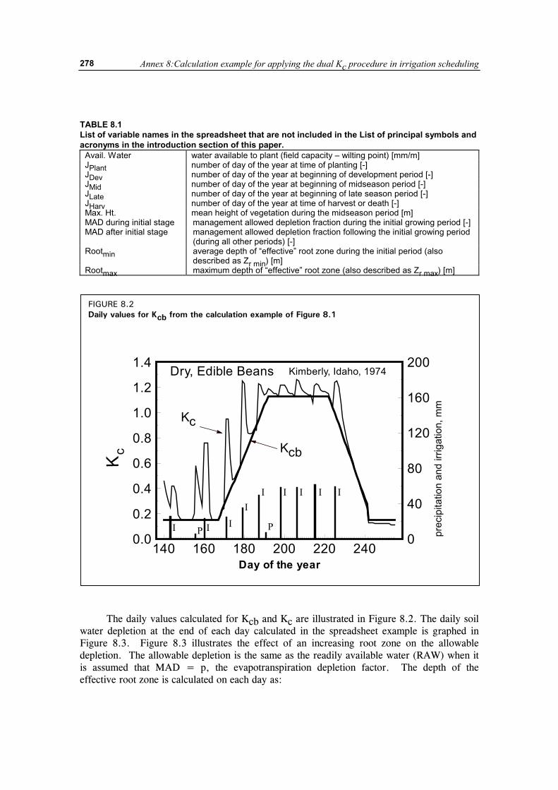
Annex 8:Calculation example for applying the dual Kc procedure in irrigation scheduling
278
TABLE 8.1 List of variable names in the spreadsheet that are not included in the List of principal symbols and acronyms in the introduction section of this paper.
Avail. Water water available to plant (field capacity – wilting point) [mm/m] JPlant number of day of the year at time of planting [-] JDev number of day of the year at beginning of development period [-] JMid number of day of the year at beginning of midseason period [-] JLate number of day of the year at beginning of late season period [-] JHarv number of day of the year at time of harvest or death [-] Max. Ht. mean height of vegetation during the midseason period [m] MAD during initial stage management allowed depletion fraction during the initial growing period [-] MAD after initial stage management allowed depletion fraction following the initial growing period
(during all other periods) [-] Rootmin average depth of “effective” root zone during the initial period (also
described as Zr min) [m] Rootmax maximum depth of “effective” root zone (also described as Zr max) [m]
The daily values calculated for Kcb and Kc are illustrated in Figure 8.2. The daily soil water depletion at the end of each day calculated in the spreadsheet example is graphed in Figure 8.3. Figure 8.3 illustrates the effect of an increasing root zone on the allowable depletion. The allowable depletion is the same as the readily available water (RAW) when it is assumed that MAD = p, the evapotranspiration depletion factor. The depth of the effective root zone is calculated on each day as:
FIGURE 8.2 Daily values for Kcb from the calculation example of Figure 8.1
140 160 180 200 220 2400.0
0.2
0.4
0.6
0.8
1.0
1.2
1.4
0
40
80
120
160
200
Day of the year
Kc
prec
ipita
tion
and
irrig
atio
n, m
m
Dry, Edible Beans Kimberly, Idaho, 1974
I
I
I
I I II
P PI
I
Kc
Kcb
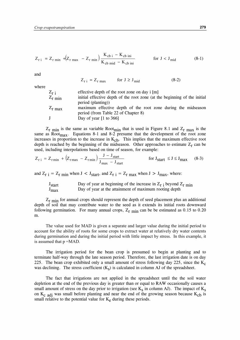
Crop evapotranspiration
279
( ) midinicbmidcb
inicbicbminrmaxrminrir JJfor
KK
KKZZZZ <
−
−−+= (8-1)
and midmaxrir JJforZZ ≥= (8-2)
where Zr i effective depth of the root zone on day i [m] Zr min initial effective depth of the root zone (at the beginning of the initial
period (planting)) Zr max maximum effective depth of the root zone during the midseason
period (from Table 22 of Chapter 8) J Day of year [1 to 366] Zr min is the same as variable Rootmin that is used in Figure 8.1 and Zr max is the same as Rootmax. Equations 8-1 and 8-2 presume that the development of the root zone increases in proportion to the increase in Kcb. This implies that the maximum effective root depth is reached by the beginning of the midseason. Other approaches to estimate Zr can be used, including interpolations based on time of season, for example:
( )startmax
startminrmaxrminrir JJ
JJZZZZ
−−
−+= for Jstart ≤ J ≤ Jmax (8-3)
and Zr i = Zr min when J < Jstart, and Zr i = Zr max when J > Jmax, where: Jstart Day of year at beginning of the increase in Zr i beyond Zr min Jmax Day of year at the attainment of maximum rooting depth Zr min for annual crops should represent the depth of seed placement plus an additional depth of soil that may contribute water to the seed as it extends its initial roots downward following germination. For many annual crops, Zr min can be be estimated as 0.15 to 0.20 m. The value used for MAD is given a separate and larger value during the initial period to account for the ability of roots for some crops to extract water at relatively dry water contents during germination and during the initial period with little impact by stress. In this example, it is assumed that p =MAD. The irrigation period for the bean crop is presumed to begin at planting and to terminate half-way through the late season period. Therefore, the last irrigation date is on day 225. The bean crop exhibited only a small amount of stress following day 225, since the Kc was declining. The stress coefficient (Ks) is calculated in column AJ of the spreadsheet. The fact that irrigations are not applied in the spreadsheet until the the soil water depletion at the end of the previous day is greater than or equal to RAW occasionally causes a small amount of stress on the day prior to irrigation (see Ks in column AJ). The impact of Ks on Kc adj was small before planting and near the end of the growing season because Kcb is small relative to the potential value for Ke during these periods.
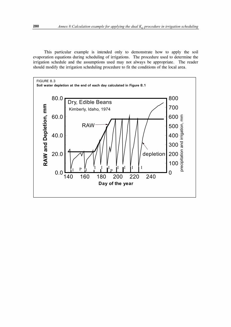
Annex 8:Calculation example for applying the dual Kc procedure in irrigation scheduling
280
This particular example is intended only to demonstrate how to apply the soil evaporation equations during scheduling of irrigations. The procedure used to determine the irrigation schedule and the assumptions used may not always be appropriate. The reader should modify the irrigation scheduling procedure to fit the conditions of the local area.
FIGURE 8.3 Soil water depletion at the end of each day calculated in Figure 8.1
140 160 180 200 220 2400.0
20.0
40.0
60.0
80.0
0100200300400500600700800
Day of the year
RA
W a
nd D
eple
tion,
mm
prec
ipita
tion
and
irrig
atio
n, m
m
Dry, Edible BeansKimberly, Idaho, 1974
I II I I IIP PI I
RAW
depletion
Crop evapotranspiration
281
Bibliography
A. BASIC CONCEPTS AND DEFINITIONS Allen, R.G., Smith, M., Perrier, A., and Pereira, L.S. 1994a. An update for the definition of reference
evapotranspiration. ICID Bulletin. 43(2). 1-34.
Jensen, M.E., Burman, R.D., and Allen, R.G. (ed). 1990. Evapotranspiration and Irrigation Water Requirements. ASCE Manuals and Reports on Engineering Practices No. 70., Am. Soc. Civil Engrs., New York, NY, 360 p.
Monteith, J.L., 1965. Evaporation and Environment. 19th Symposia of the Society for Experimental Biology, University Press, Cambridge, 19:205-234.
Monteith, J.L. 1973. Principles of Environmental Physics, Edward Arnold, London.
Monteith, J.L. and Unsworth, M.H. 1990. Principles of Environmental Physics, 2nd ed., Edward Arnold, London.
Penman, H. L. 1948. "Natural evaporation from open water, bare soil and grass." Proc. Roy. Soc. London, A193, 120-146.
Penman, H.L. 1963. Vegetation and hydrology. Tech. Comm. No. 53, Commonwealth Bureau of Soils, Harpenden, England. 125 p.
Pereira, L.S., Perrier, A., Allen, R.G. and Alves, I. 1996. Evapotranspiration: Review of concepts and future trends. J. Irrig. And Drain. Engrg., ASCE 25. (in press).
Perrier, A. 1978. Importance des définitions de l'évapotranspiration dans le domaine pratique de la mesure, de l'estimation of de la notion de coefficients culturaux. XV' Journal of Hydraulics, Société Hydrotechnique de France, Question IV, Rapport 1:1-7 (in French).
Perrier, A. 1982. Land surface processes: vegetation. pp. 395-448 in P.S. Eagleson (Editor), Land Surface Processes in Atmospheric General Circulation Models. Cambridge Univ. Press, Cambridge, Mass.
Perrier, A. 1985. Updated evapotranspiration and crop water requirement definitions. In: Perrier, A. and Riou, C.(eds) Crop Water Requirements (ICID Int. Conf., Paris, Sept. 1984). INRA, Paris: 885-887.
Rijtema, P.E., (1965). “Analysis of actual evapotranspiration.” Agric. Res. Rep. No. 69, Centre for Agric. Publ. and Doc., Wageningen.
Slatyer, R.O. and McIlroy, I.C. 1961. Evaporation and the principle of its measurement. In: Practical Meteorology, CSIRO (Australia) and UNESCO, Paris.
Smith, M., Allen, R.G., Monteith, J.L., Perrier, A., Pereira, L., and Segeren, A. 1992. Report of the expert consultation on procedures for revision of FAO guidelines for prediction of crop water requirements. UN-FAO, Rome, Italy, 54 p.
References
282
B. ET EQUATIONS Allen, R.G. 1986. A Penman for all seasons. J. Irrig. and Drain. Engrg. 112(4):348-368.
Allen, R.G. 1992. Evaluation of a temperature difference method for computing grass reference evapotranspiration. Report submitted to UN-FAO Water Resources Development and Management Service, Land and Water Dev. Div., Rome. 50 p.
Allen, R.G., 1995b. Evaluation of procedures for estimating grass reference evapotranspiration using air temperature data only. Report prepared for FAO, Water Resources Development and Management Service, FAO, Rome.
Allen, R.G. and Pruitt, W.O. 1986. Rational use of the FAO Blaney-Criddle formula. J. Irrig. and Drain. Engrg., ASCE 112(IR2):139-155.
Allen, R.G. and Pruitt, W.O. 1991. FAO-24 reference evapotranspiration factors. J. Irrig. and Drain. Engrg., ASCE 117(5):758-773.
Allen, R.G., Pruitt, W.O., Businger, J.A., Fritschen, L.J., Jensen, M.E., and Quinn, F.H. 1996. Chapter 4 “Evaporation and Transpiration” in ASCE Handbook of Hydrology. New York, NY. p. 125-252.
Batchelor, C.H. 1984. The accuracy of evapotranspiration functions estimated with the FAO modified Penman equation. Irrig. Science 5(4): 223-234.
Blaney, H.F. and Criddle, W.D. 1950. Determining water requirements in irrigated areas from climatological and irrigation data. USDA Soil Conserv. Serv. SCS-TP96. 44 pp.
Brutsaert, W.H., 1982. Evaporation into the Atmosphere. R. Deidel Publishing Company, Dordrecht, Holland.
Burman, R. and Pochop, L.O. 1994. Evaporation, Evapotranspiration and Climatic Data. Elsevier Science B.V., Amsterdam.
Businger, J.A. 1956. Some remarks on Penman’s equations for the evapotranspiration. Netherlands J. Agric. Sci. 4: 77.
Castrignanò, A., de Caro, A., and Tarantino, E. 1985. Verifica sulla validità di alcuni metodi empirici di stima dell'evapotraspirazione potenziale nel Metapontino. (Verification of validity of several empirical methods of estimating potential evapotranspiration in southern Italy). L'Irrigazione XXXII (4):23-28 (in Italian).
Chiew, F.H.S., N.N. Kamadalasa, H.M. Malano and McMahon, T.A. 1995. Penman-Monteith, FAO-24 reference crop evapotranspiration and class-A pan data in Australia. Agric. Water Management 28: 9-21.
Choisnel, E., de Villele, O., and Lacroze, F. 1992. Une approche uniformisée du calcul de l'évapotranspiration potentielle pour l'ensemble des pays de la Communauté Européenne, Com. Commun. Européennes, EUR 14223 FR, Luxembourg, 176 p.
Christiansen, J.E. 1968. Pan evaporation and evapotranspiration from climatic data. J. Irrig. and Drain. Div., ASCE 94:243-265.
Cuenca, R.H. and Nicholson, M.T. 1982. Application of the Penman equation wind function. J. Irrig. and Drn. Engrg. Div., ASCE 108(IR1):13-23.
Doorenbos, J. and Kassam, A.H. 1979. Yield response to water. FAO Irrig. and Drain. Paper No. 33, FAO, Rome, Italy. 193 pp.
Doorenbos, J. and Pruitt, W.O. 1975. Guidelines for predicting crop water requirements, Irrigation and Drainage Paper 24, Food and Agriculture Organization of the United Nations, Rome, 179 p.
Feddes, R.A. 1987. Crop factors in relation to Makkink reference crop evapotranspiration. Tech. Bull. Inst. for Land and Water Management Research. No. 67, pp. 33-45.
Crop evapotranspiration
283
Frére, M. and Popov, G.F. 1979. Agrometeorological crop monitoring and forecasting. FAO Plant Production and Protection Paper 17. FAO, Rome, Italy., pp 38-43.
Frevert, D.K., Hill, R.W., and Braaten, B.C. 1983. Estimation of FAO evapotranspiration coefficients. J. Irrig. and Drain Engrg., ASCE 109(IR2):265-270.
Gunston, H. and Batchelor, C.H. 1983. A comparison of the Priestley-Taylor and Penman methods for estimating reference crop evapotranspiration in tropical countries. Agric. Water Man. 6:65-77.
George, W., Pruitt, W.O., and Dong, A. 1985. Evapotranspiration modeling. In: California Irrigation Management Information System, Final Report, by R. Snyder, D.W. Henderson, Pruitt, W.O., and Dong, A. Calif. Dept. Water Resour. Contract. No. B53812. Land, Air and Water Resources Pap. 10013-A, Univ. Calif., Davis, III-36 to III-59.
Gosse, G., Perrier, A., and Itier, B. 1977. Etude de l'évapotranspiration réelle d'une culture de blé dans le bassin parisien. Ann. Agron. 28(5):521-541. (in French).
Hargreaves, G.H. 1983. Discussion of 'Application of Penman wind function' by Cuenca, R.H. and Nicholson, M.J. J. Irrig. and Drain. Engrg., ASCE 109(2):277-278.
Hargreaves, G.L., Hargreaves, G.H., and Riley, J.P. 1985. Agricultural benefits for Senegal River Basin. J. Irrigation and Drainage Engr., ASCE 111:113-124.
Hashemi, F. and Habibian, M.T. 1979. Limitations of temperature based methods in estimating crop evapotranspiration in arid-zone agricultural development project. Agric. Meteorol. 20: 237-247.
Hatfield, J.L. and Fuchs, M. 1990. Evapotranspiration models. Chapter 3, pp 33-59 in Management of Farm Irrigation Systems (G.J. Hoffman, T.A. Howell, and K.H. Solomon (ed)), ASAE, St. Joseph, Michigan.
Howell, T.A., Schneider, A.D., and Jensen, M.E. 1991. History of lysimeter design and use for evapotranspiration measurements. In Allen, R.G., Howell, T.A., Pruitt, W.O., Walter, I.A., and Jensen, M.E. (Editors), Lysimeters for Evapotranspiration and Environmental Measurements, ASCE, New York, NY p. 1-9.
Itier, B. and Perrier, A. 1976a. Presentation d'une étude analytique de l'advection: I. Advection lie'e aux variations horizontales de concentration et de temperature. Ann. Agron. 27(2):111-140.
Itier, B., Brunet, Y., Mcaneney, K.J., and Lagouarde, J.P. 1994. Downwind evolution of scalar fluxes and surface resistance under conditions of local adection. Part I: A reappraisal of boundary conditions. Agric. and For. Meteorol. 71: 211-255.
Itier, B. 1996. Measurement and estimation of evapotranspiration. In: Pereira, L.S., Feddes, R.A., Gilley, J.R., Leseffre, B. (eds) Sustainability of Irrigated Agriculture. Kluwer Acad. Publ., Dordrecht, pp. 171-191.
Jensen, M.E. and Haise, H.R. 1963. Estimating evapotranspiration from solar radiation. J.Irrig. and Drain. Div., ASCE, 89:15-41.
Jensen, M.E. 1974. (ed.) Consumptive use of water and irrigation water requirements. Rep. Tech. Com. on Irrig. Water Requirements, Irrig. and Drain. Div., ASCE, 227 pp.
Jensen, M.E., Burman, R.D., and Allen, R.G. (ed). 1990. Evapotranspiration and Irrigation Water Requirements. ASCE Manuals and Reports on Engineering Practices No. 70., Am. Soc. Civil Engrs., New York, NY, 360 p.
Katerji, N. and Perrier, A. 1983. Modélization de l'évapotranspiration réelle ETR d'une parcelle de luzerne: rôle d'un coefficient cultural. Agronomie 3(6):513-521 (in French).
Makkink, G.F. 1957. Testing the Penman formula by means of lysimeters. J. Inst. Water Engng. 11 (3): 277-288.
References
284
McNaughton, K.G. and Jarvis, P.G. 1984. Using the Penman-Monteith equation predictively. Agricultural Water Management 8:263-278.
Monteith, J.L. 1973. Principles of Environmental Physics, Edward Arnold, London.
Monteith, J.L. 1981. Evaporation and surface temperature. Quart. J. Roy. Meteorol. Soc. 107:1-27.
Monteith, J.L. 1985. Evaporation from land surfaces: progress in analysis and prediction since 1948. pp. 4-12 in Advances in Evapotranspiration, Proceedings of the ASAE Conference on Evapotranspiration, Chicago, Ill. ASAE, St. Joseph, Michigan.
Pelton, W.L., King, K.M. and Tanner, C.B. 1960. An evaluation of the Thornthwaite and mean temperature methods for determining potential evapotranspiration. Agron. J. 52: 387-395.
Penman, H. L. 1948. "Natural evaporation from open water, bare soil and grass." Proc. Roy. Soc. London, A193, 120-146.
Penman, H.L. 1963. Vegetation and hydrology. Tech. Comm. No. 53, Commonwealth Bureau of Soils, Harpenden, England. 125 pp.
Pereira, L.S. and Smith, M. 1989. Proposed procedures for revision of guidelines for predicting crop water requirements. Land and Water Use Div., FAO Rome, 36 p.
Phene, C.J., Clark, D.A. and Cardon, G.E. 1996. Real time calculation of crop evapotranspiration using an automated pan evaporation system. In: Camp, C.R., Sadler, E.J. and Yoder, R.E. (eds.). Evaporation and Irrigation Scheduling, ASCE: 189-194.
Piper, B.S. 1989. Sensitivity of Penman estimates of evaporation to errors in input data. Ag. Water Man. 15:279-300.
Priestley, C.H.B. and Taylor, R.J. 1972. On the assessment of surface heat flux and evaporation using large scale parameters. Mon. Weath. Rev., 100: 81-92. Pruitt, W.O. (1996). “Empirical method of estimating evapotranspiration using primarily evaporation pans.” Proc. Conf. on Evapotanspiration and its Role in Water Resources Management. Chicago. Dec. pp. 57-61. Stewart, J.B. 1983. A discussion of the relationships between the principal forms of the combination equation for estimating evapotranspiration. Ag. Meteorol. 30:111-127.
Rosenberg, N.J., Blad, B.L. and Verma, S.B. 1983. Microclimate. The Biological Environment (2nd edition). J. Wiley, New York.
Seemann, J., Chirkov, Y.I., Lomas, J. and Primault, B., 1979. Agrometeorology.Springer Verlag, Berlin, Heidelberg.
Seguin, B., Brunet, Y., and Perrier, A. 1982. Estimation of evaporation: a review of existing methods and recent developments. in European Geologic Society Symposium on Evaporation. Leeds, U.K., August, 1982, 21 p.
Sharma, M.L. 1985. Estimating evapotranspiration. p. 213-281 in Adv. in Irrigation, Vol III, D. Hillel (Editor)., Academic Press, New York.
Stewart, J.B. 1983. A discussion of the relationships between the principal forms of the combination equation for estimating evaportranspirations. Ag. Meteorol. 30:111-127.
Tanner, C.B. and Pelton, W.L. 1960. Potential evapotranspiration estimates by the approximate energy balance of Penman. J. Geophysical Res. 65(10):3391-3413.
Tanner, C.B. and Fuchs, M. 1968. Evaporation from unsaturated surfaces: a generalized combination equation. J. Geophysical Res. 73(4):1299-1304.
Thompson, N., Barrie, I.A., and Ayles, M. 1981. The Meteorological Office rainfall and evaporation calculation system: MORECS. Hydrological Memorandum 45, Hydrometeorological Services, London, 66 p.
Crop evapotranspiration
285
Thornthwaite, C.W. 1948. An approach toward a rational classification of climate. Geograph. Rev., 38, 55.
Turc, L. 1961. Evaluation des besoins en eau d'irrigation, evapotranspiration potentielle, formule climatique simplifice et mise a jour. (in French). Ann. Agron. 12:13-49.
Watts, P.J. and Hancock, N.H. 1985. Evaporation and potential evaporation- a practical approach for agricultural engineers. Mech. Engrg. Trans. 10(4):231-240 plus discussions during 1986.
Wright, J.L. 1982. New evapotranspiration crop coefficients. J. irrig. and Drain. Div., ASCE, 108 (IR2): 57-74.
Wright, J.L. 1988. Daily and seasonal evapotranspiration and yield of irrigated alfalfa in southern Idaho. Agron. J. 80: 662-669.
C. ET AND WEATHER MEASUREMENT Allen, R.G. 1996. Assessing integrity of weather data for use in reference evapotranspiration estimation. J.
Irrig. and Drain. Engng. Div., ASCE 122(2): 97-106.
Allen, R.G., Pruitt, W.O., and Jensen, M.E. 1991. Environmental requirements for lysimeters. pp. 170-181 in Allen, R.G., Howell, T.A., Pruitt, W.O., Walter, I.A., and Jensen, M.E. (Editors). Lysimeters for Evapotranspiration and Environmental Measurements. Proc. of the ASCE Int. Symp. on Lysimetry, Honolulu, HA, ASCE, New York, NY.
Bastiaanssen, W.G.M. 1995. Regionalization of surface flux densities and moisture indicators in composite terrain. Doctoral thesis, Wageningen Agricultural University, Wageningen, 273 pp.
Beard, J.R. 1985. An assessment of water use by turfgrass. p. 45-60 in Gibeault, V.A. and Cockerham, S.T. (Editors). Turfgrass Water Conservation. Publ. 21405, Univ. Calif., Div. of Agric. and Nat. Resour., Berkley, Calif.
Biran, I., Bravdo, B., Bushkin-Harav, I., and Rawitz, E. 1981. Water consumption and growth rate of 11 turfgrasses as affected by mowing height, irrigation frequency and soil moisture. Agron. J. 73:85-90.
Blad, B.L. and Rosenberg, N.J. 1974. Lysimetric calibration of the Bowen-ratio energy balance method for evapotranspiration estimation in the Central Great plains. J. App. Meteorol. 13(2):227-236.
Brutsaert, W.H., 1982. Evaporation into the Atmosphere. R. Deidel Publishing Company, Dordrecht, Holland.
Businger, J.A. 1988. “A note on the Businger-Dyer profiles.” Boundary-Layer Meteorol. 42: 145-151.
Businger, J.A. and Yaglom, A.M. 1971. “Introduction to Obukhov’s paper on ‘Turbulence in an atmosphere with a non-uniform temperature’,” Boundary-Layer Meteorol. 2: 3-6.
Campbell, G.S. 1977. An Introduction to Environmental BioPhysics. Springer Verlag, N.Y. 159 p.
Carrijo, O.A. and Cuenca R.H., 1992. Precision of evapotranspiration estimates using neutron probe. J. Irrig. and Drain. Engrg., ASCE 118 (6): 943-953.
Dolman, A.J. and Stewart, J. B. 1987. Modelling forest transpiration from climatological data. In: R.H. Swanson, P.Y. Bernier and P.D. Woodard (eds) Forest Hydrology and Watershed Management, IAHS Publ. 167: 319-327.
Fritschen, L.J. and Fritschen, C.L. 1991. Design and evaluation of net radiometers. Paper presented at the 7th Symp. on Meteorol. Observations and Instrumentation, Jan. 13-18, 1991., New Orleans, La., U.S.A. 5 p.
References
286
Gash, J.H.C., Shuttleworth, W.J., Lloyd, C.R., André, J.C., Goutorbe, J.P., and Gelpe, J. 1989. Micrometeorological measurements in Les Landes forest during HAPEX-MOBILHY. Ag. and For. Meteorol. 46:131-147.
Grant, D.R. 1975. Comparison of evaporation from barley with Penman estimates. Agric. Meteorol. 15: 49-60.
Grebet, P. and Cuenca, R.H. 1991. History of lysimeter design and effects of environmental disturbances. in Allen, R.G., Howell, T.A., Pruitt, W.O., Walter, I.A., and Jensen, M.E. (Editors), Lysimeters for Evapotranspiration and Environmental Measurements, ASCE, New York, NY p. 10-18.
Itier, B. and Perrier, A. 1976a. Presentation d'une étude analytique de l'advection: I. Advection lie'e aux variations horizontales de concentration et de temperature. Ann. Agron. 27(2):111-140.
Itier, B., Brunet, Y., Mcaneney, K.J., and Lagouarde, J.P. 1994. Downwind evolution of scalar fluxes and surface resistance under conditions of local adection. Part I: A reappraisal of boundary conditions. Agric. and For. Meteorol. (in press).
Itier, B. 1996. Measurement and estimation of evapotranspiration. In: Pereira, L.S., Feddes, R.A., Gilley, J.R., Leseffre, B. (eds) Sustainability of Irrigated Agriculture. Kluwer Acad. Publ., Dordrecht, pp. 171-191.
Kessler, J., Perrier, A. and Pescara, C. de, 1990. La Météo Agricole. Météole, (Pau).
Kizer, M.A., Elliott, R.L. and Stone, J.F. 1990. Hourly ET model calibration with eddy flux and energy balance data. J. Irrig. and Drain. Engrg., ASCE 116(2):172-181.
Marsh, A.W., Strohman, R.A., Spaulding, S., Younger, V., and Gibeault, V. 1980. Turf grass irrigation research at the University of California: warm and cool season grasses tested for water needs. Irrig. J., July/August. 20-21, 32-33.
Meyer, W.S. and Mateos, L. 1990. Effects of soil type on soybean crop water use in weighing lysimeters. II. effect of lysimeter canopy height discontinuity on evaporation. Irrig. Sci. 11:233-237.
Neale, C.M.U., Kruse, E.G., and Yoder, R.E. 1991. Field experience with hydraulic weighing lysimeters. in Allen, R.G., Howell, T.A., Pruitt, W.O., Walter, I.A., and Jensen, M.E. (Editors), Lysimeters for Evapotranspiration and Environmental Measurements, ASCE, New York, NY p. 160-169.
Pearce, A.J., Gash, J.H.C., and Stewart, J.B. 1980. Rainfall interception in a forest stand estimated from grassland meteorological data. J. Hydrol., 46:147-163.
Perrier, A., Itier, B., Bertolini, J.M., and Katerji, N. 1976. A new device for continuous recording of the energy balance of natural surfaces. Agric. Meteor. 16(1):71-85.
Perrier, A. and Tuzet, A. 1991. Land surface processes: Description, theoretical approaches, and physical laws underlying their measurements. pp. 145-155 in Schmugge, T.J. and Andre, J.-C. (eds) Land Surface Evaporation: Measurement and Parameterization. Springer-Verlag. Berlin.
Perrier, A., Archer, P., and de Pablos, B. 1974. Etude de l'évapotranspiration réelle et maximele de diverses cultures. I: Dispositif et mesure. Ann. Agron. 25(3:229-243.
Perrier, A., Katerji, N., Gosse, G., and Itier, B. 1980. Etude "in situ" de l'evapotranspiration reelle d'une culture de ble. (In situ study of evapotranspiration rates for a wheat crop). Agric. Meterol. 21:295-311. (in French).
Pruitt, W.O., Morgan, D.L., and Lourence, F.J. 1973. Momentum and mass transfers in the surface boundary layer. Quart. J. Roy. Meteorol. Soc. 99:370-386.
Pruitt, W.O. 1991. Development of crop coefficients using lysimeters. pp. 182-190 in Allen, R.G., Howell, T.A., Pruitt, W.O., Walter, I.A., and Jensen, M.E. (Editors). Lysimeters for
Crop evapotranspiration
287
Evapotranspiration and Environmental Measurements. Proc. of the ASCE Int. Symp. on Lysimetry, Honolulu, HA, ASCE, New York, NY.
Pruitt, W.O. and Lourence, F. J. 1985. Experiences in lysimetry for ET and surface drag measurements. pp. 51-69 in: Advances in Evapotranspiration, ASAE, St. Joseph, MI.
Rosenberg, N.J., Blad, B.L. and Verma, S.B. 1983. Microclimate. The Biological Environment (2nd edition). J. Wiley, New York.
Schulze, K. 1995. Report of expert meeting for the preparation of an intercomparison of instruments and procedures for measurement and estimation of evaporation and evapotranspiration. World Meteorological Organization, Commission for Instruments and Methods of Observation. Geneva, Switzerland. 30 p.
Seemann, J., Chirkov, Y.I., Lomas, J. and Primault, B., 1979. Agrometeorology.Springer Verlag, Berlin, Heidelberg.
Shuttleworth, W.J. 1993. Evaporation. In: D.R. Maidment (ed) Handbook of Hydrology. McGraw Hill, New York: 4.1-4.53.
Shuttleworth, W.J. and Wallace, J.S. 1985. Evaporation from sparse crops - an energy combination theory. Quart. J. Roy Meteorol. Soc. 111: 839-853.
Stringer, W.C., Wolf, D.D., and Baser, R.E. 1981. Summer regrowth of tall fescue: stubble characteristics and microenvironment. Agron. J. 73:96-100.
Slatyer, R.O. and McIlroy, I.C. 1961. Evaporation and the principle of its measurement. In: Practical Meteorology, CSIRO (Australia) and UNESCO, Paris.
Stewart, J.B. and Gay, L.W. 1989. Preliminary modelling of transpiration from the FIFE stie in Kansas. Agric. and For. Meteorol. 48:305-315.
Tarantino, E. 1991. Grass reference measurements in Italy. in Allen, R.G., Howell, T.A., Pruitt, W.O., Walter, I.A., and Jensen, M.E. (Editors), Lysimeters for Evapotranspiration and Environmental Measurements, ASCE, New York, NY p. 200-209.
Thom, A.S., Thony, J.L., and Vauclin, M. 1981. On the proper employment of evaporation pans and atmometers in estimating potential transpiration. Quart. J. Roy. Meteorol. Soc., 107: 711-736.
Walter, I.A., Siemer, E., Dirks, L.R., Quinian, J.P., and Burman, R.D. 1991. Lysimeters vs. buffer areas: evapotranspiration and agronomic comparisons. in Allen, R.G., Howell, T.A., Pruitt, W.O., Walter, I.A., and Jensen, M.E. (Editors), Lysimeters for Evapotranspiration and Environmental Measurements, ASCE, New York, NY p. 10-18.
Wehner, D.J. and Watschke, T.L. 1981. Heat tolerance of Kentucky bluegrasses, perennial ryegrasses, and annual bluegrass. Agron. J. 73:79-84.
WMO 1983 Guide to Meteorological Instruments and Observing Practices. WMO nº 8 (fifth edition), Geneva.
Wright, J.L. 1991. Using lysimeters to develop evapotranspiration crop coefficients. in Allen, R.G., Howell, T.A., Pruitt, W.O., Walter, I.A., and Jensen, M.E. (Editors), Lysimeters for Evapotranspiration and Environmental Measurements, ASCE, New York, NY p. 191-199.
D. PARAMETERS IN ET EQUATIONS Allen, R.G., Jensen, M.E., Wright, J.L., and Burman, R.D. 1989. Operational estimates of reference
evapotranspiration. Agron. J. 81:650-662.
Allen, R.G., Smith, M., Perrier, A., and Pereira, L.S. 1994a. An update for the definition of reference evapotranspiration. ICID Bulletin. 43(2). 1-34.
References
288
Allen, R.G., Smith, M., Pereira, L.S., and Perrier, A. 1994b. An update for the calculation of reference evapotranspiration. ICID Bulletin, 43 (2): 35-92.
Allen, R.G. 1995a. Evaluation of procedures for estimating mean monthly solar radiation from air temperature. Report prepared for FAO, Water Resources Development and Management Service, FAO, Rome.
Bosen, J.F. 1958. An approximation formula to compute relative humidity from dry bulb and dew point temperatures. Monthly Weather Rev. 86(12):486.
Brunt, D. 1939. Physical and dynamical meteorology, Univ. Press, Cambridge. 400 pp.
Brunt, D. 1952. Physical and dynamical meteorology, 2nd ed., Univ. Press, Cambridge. 428 pp.
Brutsaert, W.H., 1982. Evaporation into the Atmosphere. R. Deidel Publishing Company, Dordrecht, Holland.
Burman, R.D., Jensen, M.E., and Allen, R.G. 1987. Thermodynamic factors in evapotranspiration. In: James, L.G. and M.J. English (editors), Proc. Irrig. and Drain. Spec. Conf., ASCE, Portland, Ore., p. 28-30.
Burman, R. and Pochop, L.O. 1994. Evaporation, Evapotranspiration and Climatic Data. Elsevier Science B.V., Amsterdam.
Businger, J.A. 1988. “A note on the Businger-Dyer profiles.” Boundary-Layer Meteorol. 42: 145-151.
Choudhury, B.J., Idso, S.B., and Reginato, R.J. 1987. Analysis of an empirical model for soil heat flux under a growing wheat crop for estimating evaporation by an infrared temperature based energy balance equation. Agric. for. Meteorol. 39:283-297.
Clothier, B.E., Clawson, K.L., Pinter, P.J., Moran, M.S., Reginato, R.J., and Jackson, R.D. 1986. Estimates of soil heat flux from net radiation during the growth of alfalfa. Agric. For. Meteorol 37:319-329.
Duffie, J.A. and Beckman, W.A. 1991. Solar engineering of thermal processes. 2nd Ed., John Wiley and sons, New York. 994 p. Harrison, L.P. 1963. Fundamentals concepts and definitions relating to humidity. In Wexler, A (Editor) Humidity and moisture Vol 3, Reinhold Publishing Co., N.Y.
Dyer, A.J. 1974. A reviewof flux-profile relationships. Boundary Layer Meterol. 7: 363-372.
Dyer, A.J. and Hicks, B.B., 1970. Flux-gradient relationships in the constant flux layer. Quart. J. Roy. Meteorol. Soc. 96: 715-721.
Frevert, D.K., Hill, R.W., and Braaten, B.C. 1983. Estimation of FAO evapotranspiration coefficients. J. Irrig. and Drain Engrg., ASCE 109(IR2):265-270.
Garratt, J.R. (1992). The atmospheric boundery layer. Cambridge Univ. Press, 316 p.
Garratt, J.R. and Hicks, B.B. 1973. Momentum, heat and water vapour transfer to and from natural and artificial surfaces. Quart. J. Roy. Meteorol. Soc. 99: 680-687.
George, W., Pruitt, W.O., and Dong, A. 1985. Evapotranspiration modeling. In: California Irrigation Management Information System, Final Report, by R. Snyder, D.W. Henderson, Pruitt, W.O., and Dong, A. Calif. Dept. Water Resour. Contract. No. B53812. Land, Air and Water Resources Pap. 10013-A, Univ. Calif., Davis, III-36 to III-59.
Gosse, G., Perrier, A., and Itier, B. 1977. Etude de l'évapotranspiration réelle d'une culture de blé dans le bassin parisien. Ann. Agron. 28(5):521-541. (in French).
Harrison, L.P. 1963. Fundamentals concepts and definitions relating to humidity. In Wexler, A (Editor) Humidity and moisture Vol 3, Reinhold Publishing Co., N.Y.
Hashemi, F. and Habibian, M.T. 1979. Limitations of temperature based methods in estimating crop evapotranspiration in arid-zone agricultural development project. Agric. Meteorol. 20: 237-247.
Crop evapotranspiration
289
Hatfield, J.L. and Fuchs, M. 1990. Evapotranspiration models. Chapter 3, pp 33-59 in Management of Farm Irrigation Systems (G.J. Hoffman, T.A. Howell, and K.H. Solomon (ed)), ASAE, St. Joseph, Michigan.
Hottel, H.C. 1976. A simple model for estimating the transmittance of direct solar radiation through clear atmospheres. Solar Energy 18:129.
Idso, S.B. and Jackson, R.B. 1969. Thermal radiation from the atmosphere. J. Geophys. Res. 74:5397-5403.
Jensen, J.R. 1988. Effect of asymmetric, daily air temperature and humidity waves on calculation of reference evapotranspiration. Proc. European Economic Community Workshop on Management of Water Resources in Cash Crops and in Alternative Production Systems. Brussels, Belg. 24-25 Nov., 1988. 12 p.
List, R.J. 1984. Smithsonian Meteorological Tables, 6th rev. ed., Smithsonian Institution, Washington D.C., U.S.A. 539 p.
Liu, B.Y.H., and Jorden, R.C. 1960. The interrelationship and characteristic distribution of direct diffuse and total solar radiation. Solar Energy 4(3):1-19.
Matias P.G.M. 1992. SWATCHP, a model for a continuous simulation of hydrologic processes in a system vegetation - soil - aquifer - river. Ph.D.dissertation, Techn. Univ. Lisbon (in Portuguese).
Monteith, J.L. and Unsworth, M.H. 1990. Principles of Environmental Physics, 2nd ed., Edward Arnold, London.
Monteith, J.L., 1965. Evaporation and Environment. 19th Symposia of the Society for Experimental Biology, University Press, Cambridge, 19:205-234.
Murray, F.W. 1967. On the computation of saturation vapor pressure. J. Appl. Meteor. 6:203-204.
Penman, H.L. 1963. Vegetation and hydrology. Tech. Comm. No. 53, Commonwealth Bureau of Soils, Harpenden, England. 125 pp.
Pereira, L.S. and Smith, M. 1989. Proposed procedures for revision of guidelines for predicting crop water requirements. Land and Water Use Div., FAO Rome, 36 p.
Pruitt, W.O. and Doorenbos, J. 1977. Background and Development of Methods to Predict Reference Crop Evapotranspiration (ETo). Appendix II in FAO-ID-24, pp 108-119.
Seguin, B., Brunet, Y., and Perrier, A. 1982. Estimation of evaporation: a review of existing methods and recent developments. in European Geologic Society Symposium on Evaporation. Leeds, U.K., August, 1982, 21 p.
Sharma, M.L. 1985. Estimating evapotranspiration. p. 213-281 in Adv. in Irrigation, Vol III, D. Hillel (Editor)., Academic Press, New York.
Smith, M., Allen, R.G., Monteith, J.L., Pereira, L.S., Perrier, A., Pruitt, W.O. 1992. Report on the Expert Consultation on procedures for Revision of FAO Guidelines for Prediction of Crop Water Requirements. Land and Water Development Division, United Nations Food and Agriculture Service, Rome, Italy.
Tetens, O. 1930. Uber einige meteorologische Begriffe. z. Geophys. 6:297-309.
van Wijk, W.R. and de Vries, D.A. 1963. Periodic temperature variations in a homogeneous soil. In: van Wijk, W.R. (Editor). Physics of the plant environment. North-Holland Publ. Co., Amsterdam, P. 102-143.
Weiss, A. 1982. An experimental study of net radiation, its components and prediction Agron. J. 74:871-874.
WMO 1970. Guide to Hydrometeorological Practices. WMO nº 168.TP.82. Geneva
References
290
WMO 1981. Guide to Agricultural Meteorological Practices. WMO nº 134 (second edition), Geneva.
Wright, J.L. 1982. New evapotranspiration crop coefficients. J. irrig. and Drain. Div., ASCE, 108 (IR2): 57-74.
E. CROP PARAMETERS IN PM EQUATION Allen, R.G., Jensen, M.E., Wright, J.L., and Burman, R.D. 1989. Operational estimates of reference
evapotranspiration. Agron. J. 81:650-662.
Allen, R.G., Smith, M., Pereira, L.S., and Perrier, A. 1994b. An update for the calculation of reference evapotranspiration. ICID Bulletin, 43 (2): 35-92.
Allen, R.G., Vanderkimpen, P.J., and Wright, J.L. 1995. “Development of resistance parameters for operational application of the Penman-Monteith equation.” Agric. and For. Meteorol.
Alves, I.L. 1995. Modelling crop evapotranspiration. Canopy and aerodynamic resistances. Ph.D. Dissertation, ISA, Univ. Tec. Lisboa (in portuguese).
Alves, I., Perrier, A. and Pereira, L.S., 1998. Aerodynamic and surface resistances of complete over crops: How good in the “big leaf” approach? Trans. ASAE 41(2): 345-351.
Ben-Mehrez, M., Taconet, O., Vidal-Madjar, D., and Valencogne, C. 1992. “Estimation of stomatal resistance and canopy evaporation during the HAPEX-MOBILHY experiment.” Agr. and For. Meteorol. 58: 285-313.
Bevan, K. 1979. A sensitivity analysis of the Penman-Monteith actual evapotranspiration estimates. J. Hydrol. 44:169-190.
Brutsaert, W.H., 1982. Evaporation into the Atmosphere. R. Deidel Publishing Company, Dordrecht, Holland.
Businger, J.A. and Yaglom, A.M. 1971. “Introduction to Obukhov’s paper on ‘Turbulence in an atmosphere with a non-uniform temperature’,” Boundary-Layer Meteorol. 2: 3-6.
Campbell, G.S. 1977. An Introduction to Environmental BioPhysics. Springer Verlag, N.Y. 159 p.
Chamberlain, A.C., 1966. Transport of gases to and from grass and grass-like surfaces. Proc. Roy. Soc. A, 290:236-259.
DeCoursey, D.G. 1992. Evaporation and evapotranspiration processes. In: Root Zone Water Quality Model, version 1.0. Technical Documentation. GPSR, USDA-ARS, Fort Collins, Co, pp 29-74.
Dolman, A.J. and Stewart, J. B. 1987. Modelling forest transpiration from climatological data. In: R.H. Swanson, P.Y. Bernier and P.D. Woodard (eds) Forest Hydrology and Watershed Management, IAHS Publ. 167: 319-327.
Frank, A.B. 1981. Effect of leaf age and position on photosynthesis and stomatal conductance of forage grasses. Agron. J. 73:70-74.
Jarvis, P.G. 1976. The interpretation of the variations in leaf water potential and stomatal conductance found in canopies in the field. Phil. Trans. Roy. Soc., Lond., B 273:593-610.
Kelliher, F.M., Leuning, R. and Schulze, E.D. 1993. Evaporation and canopy characteristics of coniferous forests and grasslands. Oecologia 95:153-163.
Kim, J. and Verma, S.B. 1991. Modeling canopy stomatal conductance in a temperate grassland ecosystem. Agric. and For. Meteorol. 55:149-166.
Loommis, R.S. and Williams, W.A. 1969. Productivity and the morphology of crop stand patterns with leaves. In: J.D. Eastin (ed) Physiological Aspects of Crop Yield. ASA, CSSA and SSSA, Madison, WI: 27-47.
Crop evapotranspiration
291
Martin, D.L. and J.R. Gilley 1993. Irrigation Water Requirements. Chapter 2 of the SCS National Engineering Handbook, Soil Conservation Service, Washington D.C., 284 pp.
Matias P.G.M. 1992. SWATCHP, a model for a continuous simulation of hydrologic processes in a system vegetation - soil - aquifer - river. Ph.D.dissertation, Techn. Univ. Lisbon (in Portuguese).
McNaughton, K.G. and Jarvis, P.G. 1984. Using the Penman-Monteith equation predictively. Agricultural Water Management 8:263-278.
Monin, A.S. and Obukhov, A.M. 1954. “The basic laws of turbulent mixing in the surface layer of the atmosphere.” Akad. Nauk. SSSR Trud. Geofiz. Inst., No. 24. (151): 163-187.
Monteith, J.L. 1973. Principles of Environmental Physics, Edward Arnold, London.
Monteith, J.L. 1981. Evaporation and surface temperature. Quart. J. Roy. Meteorol. Soc. 107:1-27.
Monteith, J.L. 1985. Evaporation from land surfaces: progress in analysis and prediction since 1948. pp. 4-12 in Advances in Evapotranspiration, Proceedings of the ASAE Conference on Evapotranspiration, Chicago, Ill. ASAE, St. Joseph, Michigan.
Monteith, J.L. and Unsworth, M.H. 1990. Principles of Environmental Physics, 2nd ed., Edward Arnold, London.
Monteith, J.L., 1965. Evaporation and Environment. 19th Symposia of the Society for Experimental Biology, University Press, Cambridge, 19:205-234.
Paulson, C.A. 1970. The mathematical representation of wind speed and temperature profiles in the unstable atmospheric surface layer. J. Appl. Meteorol. 9: 857-861.
Perrier, A. 1982. Land surface processes: vegetation. pp. 395-448 in P.S. Eagleson (Editor), Land Surface Processes in Atmospheric General Circulation Models. Cambridge Univ. Press, Cambridge, Mass.
Perrier, A. and Tuzet, A. 1991. Land surface processes: Description, theoretical approaches, and physical laws underlying their measurements. pp. 145-155 in Schmugge, T.J. and Andre, J.-C. (eds) Land Surface Evaporation: Measurement and Parameterization. Springer-Verlag. Berlin.
Pruitt, W.O., Morgan, D.L., and Lourence, F.J. 1973. Momentum and mass transfers in the surface boundary layer. Quart. J. Roy. Meteorol. Soc. 99:370-386.
Shaw, R,H. and Pereira, A.R. 1982. Aerodynamic roughness of a plant canopy: A numerical experiment. Agric. Meteorol. 26: 51-65. Stewart, J.B. 1988. Modelling surface conductance of pine forest. Agric. and For. Meteorol. 43:19-35.
Shuttleworth, W.J. 1993. Evaporation. In: D.R. Maidment (ed) Handbook of Hydrology. McGraw Hill, New York: 4.1-4.53.
Shuttleworth, W.J. and Wallace, J.S. 1985. Evaporation from sparse crops - an energy combination theory. Quart. J. Roy Meteorol. Soc. 111: 839-853.
Smith, M., Allen, R.G., Monteith, J.L., Perrier, A., Pereira, L., and Segeren, A. 1992. Report of the expert consultation on procedures for revision of FAO guidelines for prediction of crop water requirements. UN-FAO, Rome, Italy, 54 p.
Stewart, J.B. 1989. On the use of the Penman-Monteith equation for determining areal evapotranspiration. in Estimation of Areal Evapotranspiration, IAHS Publ. no. 177:3-12.
Stewart, J.B. and Verma, S.B. 1992. Comparison of surface fluxes and conductances at two contrasting sites within the FIFE area. J. Geophysical Research 97(D17):18623-18628.
Szeicz, G. and Long, I.F. 1969. Surface resistance of crop canopies. Water Resour. Res. 5, 622-633.
Thom, A.S. 1971. Momentum absorption by vegetation. Quart. J. Roy. Meteorol. Soc. 97:414-428.
References
292
Thom, A.S. 1972. Momentum, mass and heat exchange of vegetation. Quart. J. Roy. Meteorol. Soc. 98, 124-134.
Thom, A.S. and Oliver, H.R. 1977. On Penman’s equation for estimating regional evaporation. Quart. J. Roy. Meteorol. Soc. 103: 345-357.
Thom, A.S., Setwart, J.B., Oliver, H.R. and Gash, J.H.C. 1975. Comparison of aerodynamic and energy budget estimates of fluxes over a pine forest. Quart. J. Roy. Meteorol. Soc. 101: 93-105.
van Bavel, C.H., Fritschen, L.J., and Reeves, W.E. 1963. Transpiration of sudangrass as an externally controlled process. Science 141:269-270.
Verma, S.B. 1989. Aerodynamic resistances to transfers of heat, mass and momentum. Estimation of Areal Evapotranspiration, T.A. Black, D.L. Spittlehouse, M.D. Novak and D.T. Price (ed)., IAHS Pub. No. 177. p. 13-20.
Webb, E.K. 1970. “Profile relationships: the log-linear range, and extension to strong stability.” Q.J. Roy. Met. Soc. 96: 67-90.
Wallace, J.S., Roberts, J.M., and Sivakuma, M.V.K. 1990. “The estimation of transpiration from sparse dryland millet using stomatal condutance and vegetation area indices.” Agric. and Forest Meteorol. 51: 35-49.
F. ANALYSIS OF WEATHER AND ET DATA Allen, R.G. 1996. Assessing integrity of weather data for use in reference evapotranspiration estimation. J.
Irrig. and Drain. Engng. Div., ASCE 122(2): 97-106.
Allen, R.G. and Brockway, C.E. 1983. Estimating consumptive use on a statewide basis. pp. 79-89 in Proc. 1983 Irrig. and Drain. Specialty Conf. at Jackson, WY. ASCE, New York, NY.
Allen, R.G., Brockway, C.E., and Wright, J.L. 1983. Weather station siting and consumptive use estimates. J. Water Resour. Plng. and Mgmt. Div., ASCE 109(2):134-146.
Allen, R.G. 1997. a Self-Calibrating Method for Estimating Solar Radiation from Air Temperature. J. Hydrologic Engineering, ASCE 2(2): 56-67.
Allen, R.G. and Wright, J.L. 1977. Translating Wind Measurements from Weather Stations to Agricultural Crops. J. Hydrologic Engineering, ASCE 2(1): 26-35.
Burman, R.D., Wright, J.L. and Jensen, M.E. 1975. Changes in climate and estimated evaporation across a large irrigated area in Idaho. Trans. ASAE 18 (6): 1089-1091, 1093.
Pereira, L.S. (ed.). 1998. Water and Soil Management for Sustainable Agriculture in the Huang-Huai-Hai Rivers Plain (North China). Final report of EC Research Contract CT93-250, Instituto Superior de Agronomia, Lisbon.
Pruitt, W.O. and Doorenbos, J. 1977. Background and Development of Methods to Predict Reference Crop Evapotranspiration (ETo). Appendix II in FAO-ID-24, pp 108-119.
Pruitt, W.O. and Swann, B.D. 1986. Evapotranspiration studies in N.S.W.: Daily vs. hourly meteorological data. Irrigation '86, Darling downs Institute of Advanced Education, Toowoomba, Queensland, Australia, 29 p.
Rosenberg, N.J., Blad, B.L. and Verma, S.B. 1983. Microclimate. The Biological Environment (2nd edition). J. Wiley, New York.
Snyder, R.L. and Pruitt, W.O. 1992. Evapotranspiration data management in California. Proceedings of the Irrigation and Drainage sessions of ASCE Water Forum '92, T. Engman, ed. ASCE, New York, New York. p.128-133.
Crop evapotranspiration
293
G. CROP EVAPOTRANSPIRATION Alves, I.L. 1995. Modelling crop evapotranspiration. Canopy and aerodynamic resistances. Ph.D.
Dissertation, ISA, Univ. Tec. Lisboa (in portuguese).
Bevan, K. 1979. A sensitivity analysis of the Penman-Monteith actual evapotranspiration estimates. J. Hydrol. 44:169-190.
Howell, T.A., Evett, S.R., Tolk, J.A., Schneider, A.D. and Steiner, J.L. 1996. Evapotranspiration of corn – Southern High Plains. In: Camp, C.R., Sadler, E.J. and Yoder, R.E. (eds.). Evapotranspiration and Irrigation Scheduling, ASAE: 158-166.
Jensen, M.E. 1968. Water consumption by agricultural plants. In: Kozlowski, T.T. (ed) Water Deficits and Plant Growth, vol II, Academic Press, New York: 1-22.
Jensen, M.E. 1974. (ed.) Consumptive use of water and irrigation water requirements. Rep. Tech. Com. on Irrig. Water Requirements, Irrig. and Drain. Div., ASCE, 227 pp.
Katerji, N. and Perrier, A. 1983. Modélization de l'évapotranspiration réelle ETR d'une parcelle de luzerne: rôle d'un coefficient cultural. Agronomie 3(6):513-521 (in French).
Lee, R. 1980. Forest Hydrology. Columbia Univ. Press, New York.
Perrier, A., Archer, P., and de Pablos, B. 1974. Etude de l'évapotranspiration réelle et maximele de diverses cultures. I: Dispositif et mesure. Ann. Agron. 25(3:229-243.
Perrier, A., Katerji, N., Gosse, G., and Itier, B. 1980. Etude "in situ" de l'evapotranspiration reelle d'une culture de ble. (In situ study of evapotranspiration rates for a wheat crop). Agric. Meterol. 21:295-311. (in French).
Rijtema, P.E., (1965). “Analysis of actual evapotranspiration.” Agric. Res. Rep. No. 69, Centre for Agric. Publ. and Doc., Wageningen.
Shuttleworth, W.J. 1993. Evaporation. In: D.R. Maidment (ed) Handbook of Hydrology. McGraw Hill, New York: 4.1-4.53.
H. CROP COEFFICIENTS Abtew, W. and J. Obeysekera. 1995. Lysimeter study of evapotranspiration of cattails and comparison of
three estimation methods. Trans. ASAE 38(1):121-129.
Allen, R.G., J. Prueger, and R.W. Hill. 1992. Evapotranspiration from Isolated Stands of Hydrophytes: Cattail and Bulrush. Trans ASAE 35(4):1191-1198.
Allen, R.G., R.W. Hill, and S. Vemulapali, S. 1994. Evapotranspiration Parameters for Variably-Sized Wetlands. Paper presented at the 1994 Summer Meeting of ASAE. No. 942132, 24 p. Burman, R.D., Nixon, P.R., Wright, J.L. and Pruitt, W.O. 1980 “Water requirements”p. 189-232 in Jensen, M.E. (ed) Design and operation of farm irrigation systems, Amer. Soc. Agric. Engr., St. Joseph, Mich.
Allen, R.G., Smith, M., Pereira, L.S. and Pruitt, W.O. 1997. Proposed revision to the FAO procedure for estimating crop water requirements. In: Chartzoulakes, K.S. (ed.). Proc. 2nd. Int. Sym. on Irrigation of Horticultural Crops, ISHS, Acta Hort. Vol. I: 17-33.
Doorenbos, J. and Pruitt, W. O., 1977. Crop water requirements. Irrigation and Drainage Paper No. 24, (rev.) FAO, Rome, Italy. 144 p.
Doorenbos, J. and Kassam, A.H. 1979. Yield response to water. FAO Irrig. and Drain. Paper No. 33, FAO, Rome, Italy. 193 pp.
Elliott, R. L., S. L. Harp, G. D. Grosz and M. A. Kizer. 1988. Crop Coefficients for Peanut Evapotranspiration. Agricultural Water Management15:155-164.
References
294
Feddes, R.A. 1987. Crop factors in relation to Makkink reference crop evapotranspiration. Tech. Bull. Inst. for Land and Water Management Research. No. 67, pp. 33-45.
Fereres, E., (1981). (ed.) "Drip irrigation management." Cooperative Extension, Univ. California, Berkeley, CA, Leaflet No. 21259.
Grattan, S.R., W. Bowers, A. Dong, R.L. Snyder, J.J. Carroll, and W. George. 1998. New crop coefficients estimate water use of vegetables, row crops. California Agriculture 52(1):16-21.
Howell, T.A., D.A. Bucks, D.A. Goldhamer, and J.M. Lima. 1986. "Management Principles: 4.1 Irrigation Scheduling.", in Trickle Irrigation for Crop Production: Design, Operation and Management (F.S. Nakayama and D.A. Bucks (ed)). Elsevier.
Howell, T.A., Steiner, J.L., Schneider, A.D., and Evett, S.R. 1995. Evapotranspiration of irrigated winter wheat - southern high plains. Trans. ASAE 38(3):745-759.
Jensen, M.E. 1974. (ed.) Consumptive use of water and irrigation water requirements. Rep. Tech. Com. on Irrig. Water Requirements, Irrig. and Drain. Div., ASCE, 227 pp.
Kolar, J.J. and Kohl, R.A. 1976. Irrigating alfalfa for seed production. Univ. Idaho Agric. Exp. Station Current Information Series 357., Moscow, Idaho. 3 p.
Liu, Y., Teixeira, J.L., Zhang, H.J. and Pereira, L.S. 1998. Model validation and crop coefficients for irrigation scheduling in the North China plai. Agricultural Water Management 36: 233-246.
Neale, C.M.U. 1987. Development of Reflectance Based Crop Coefficients for Corn. Unpublished PhD Dissertation, Agricultural Engineering , Colorado State University, Fort Collins, USA.
Neale, C.M.U., W.C. Bausch and D. F. Heerman. 1989. Development of reflectance-based crop coefficients for corn. Trans. ASAE 32(6):1891-1899.
Pastor, M. and Orgaz, F. 1994. Riego deficitario del olivar: Los programas de recorte de riego en olivar. Agricultura no. 746: 768-776 (in Spanish).
Pereira, L.S., Teixeira, J.L., Pereira, L.A., Ferreira, M.I., and Fernando,R.M., 1987. Simulation models of crop response to irrigation management:research approaches and needs. In: J. Feyen (ed) Simulation Models for Cropping Systems in Relation to Water Management. Commission of the European Communities, EUR 10869, Luxembourg: 19-36.
Pereira, L.S., Perrier, A., Allen, R.G. and Alves, I. 1996. Evapotranspiration: Review of concepts and future trends. In: Camp, C.R., Sadler, E.J., Yoder, R.E. (eds) Evapotranspiration and Irrigation Scheduling, ASAE: pp. 109-115.
Pruitt, W.O. 1976. "Evapotranspiration and crop coefficients for a windbreak of Monterey pine trees", personal communication, Davis, CA.
Pruitt, W.O. 1986. "Traditional methods 'Evapotranspiration research priorities for the next decade'." ASAE Paper No. 86-2629. 23 p.
Pruitt, W.O., E. Fereres, P.E. Martin, H. Singh, D.W. Henderson, R.M. Hagan, E. Tarantino, and B. Chandio. 1984. "Microclimate, evapotranspiration, and water-use efficiency for drip- and furrow-irrigated tomatoes." Proceedings 12th Congress, International Commission on Irrigation and Drainage, Ft. Collins, CO., p. 367-394.
Rogers, J.S., Allen, L.H., and Calvert, D.J. 1983. Evapotranspiration for humid regions: developing citrus grove, grass cover. Trans. ASAE, 26(6): 1778-83, 92.
Snyder, R.L., Lanini, B.J., Shaw, D.A., and Pruitt, W.O. 1989a. Using reference evapotranspiration (ETo) and crop coefficients to estimate crop evapotranspiration (ETc) for agronomic crops, grasses, and vegetable crops. Cooperative Extension, Univ. California, Berkeley, CA, Leaflet No. 21427, 12 p.
Crop evapotranspiration
295
Snyder, R.L., Lanini, B.J., Shaw, D.A., and Pruitt, W.O. 1989b. Using reference evapotranspiration (ETo) and crop coefficients to estimate crop evapotranspiration (ETc) for trees and vines. Cooperative Extension, Univ. California, Berkeley, CA, Leaflet No. 21428, 8 p.
Wright J.L. 1981. Crop coefficients for estimates of daily crop evapotranspiration. Irrig. Scheduling for Water and Energy Conservation in the 80s, ASAE, Dec. 1981.
Wright, J.L. 1982. New Evapotranspiration Crop Coefficients. J. of Irrig. and Drain. Div., ASCE, 108:57-74.
Wright, J.L. and Jensen, M.E. 1972. Peak water requirements of crops in southern Idaho. J. Irrig. and Drain. Div., ASCE 96(IR1):193-201.
Wright, J.L. 1990. Evapotranspiration data for dry, edible beans at Kimberly, Idaho., unpublished data, USDA-ARS, Kimberly, Idaho.
I. LENGTHS OF CROP GROWTH STAGES Allen, R.G. and Gichuki, F.N. 1989. Effects of Projected CO2-induced Climatic Changes on Irrigation
Water Requirements in the Great Plains States (Texas, Oklahoma, Kansas, and Nebraska). The Potential Effects of Global Climate Change on the United States: Appendix C - Agriculture. Vol. 1. EPA-230-05-89-053 (J.B. Smith and D.A. Tirpak, Eds.), U.S. Environmental Protection Agency, Office of Policy, Planning and Evaluation, Washington, D.C., (6):1-42.
Dingkuhn, M. 1994. Climatic determinants of irrigated rice performance in the Sahel. III. Characterizing environments by simulating crop phenology. Agricultural Systems (48): 435-456.
Doorenbos, J. and Pruitt, W. O., 1977. Crop water requirements. Irrigation and Drainage Paper No. 24, (rev.) FAO, Rome, Italy. 144 p.
Everson, D.O., M. Faubion and D.E. Amos 1978. "Freezing temperatures and growing seasons in Idaho." Univ. Idaho Agric. Exp. station bulletin 494. 18 p.
Kruse E.G. and Haise, H.R. 1974. "Water use by native grasses in high altitude Colorado meadows." U.S.D.A Agric. Res. Service, Western Region report ARS-W-6-1974. 60 pages
O’Halloran, T.F. 1997. Reported crop acreages by month for the Imperial Irrigation District, Imperial Irrigation District, Imperial, Calif., USA. personal communication.
Ritchie, J.T. 1991. Wheat phasic development. In: R.J. Hanks and J.T. Ritchie (Editors), Modeling Plant and Soil Systems, Agronomy Series No. 31, Am. Soc. Agron., Madison, Wisc., Chapter 3, 31-54.
Ritchie, J.T. and D.S. NeSmith. (1991). "Temperature and crop development." In: R.J. Hanks and J.T. Ritchie (Editors). Modeling Plant and Soil Systems, Agronomy Series No. 31, Am. Soc. Agron., Madison, Wisc., Chapter 2, 5-29.
Ritchie, J.T. and Johnson, B.S. (1990). "Soil and plant factors affecting evaporation." Chapter 13 of Irrigation of Agricultural Crops, (Stewart, B.A. and Nielsen, D.R (ed.)), Agronomy Series 30. Am. Soc. Agron. p. 363-390.
Snyder, R.L., Lanini, B.J., Shaw, D.A., and Pruitt, W.O. 1989a. Using reference evapotranspiration (ETo) and crop coefficients to estimate crop evapotranspiration (ETc) for agronomic crops, grasses, and vegetable crops. Cooperative Extension, Univ. California, Berkeley, CA, Leaflet No. 21427, 12 p.
Snyder, R.L., Lanini, B.J., Shaw, D.A., and Pruitt, W.O. 1989b. Using reference evapotranspiration (ETo) and crop coefficients to estimate crop evapotranspiration (ETc) for trees and vines. Cooperative Extension, Univ. California, Berkeley, CA, Leaflet No. 21428, 8 p.
References
296
Wright, J.L. 1982. New evapotranspiration crop coefficients. J. Irrig. and Drain. Div., ASCE, 108(IR2):57-74.
J. EFFECTS OF SOIL MULCHES Battikhi, A.M. and Hill, R.W. 1986. Irrigation scheduling and watermelon yield model for the Jordan
Valley. J. Agronomy and Crop Science 157:145-155.
Battikhi, A.M. and Hill, R.W. 1986. Irrigation scheduling and cantaloupe yield model for the Jordan Valley. Agricultural Water Management 15:177-187.
Ghawi, I. and Battikhi, A.M. 1986. Watermelon (Citrullus lanatus) production under mulch and trickle irrigation in the Jordan Valley. J. Agronomy and Crop Science 156:225-236.
Ghinassi, G. and Neri, L. 1998. Effect of mulching with black polyethylee sheets on sweet pepper evapotranspiration losses. In: Pereira, L.S. and Gowing, J.W. (eds.). Water and the Environment: Innovative Issues in Irrigation and Drainage. E. & F.N. Spon, London. Pp. 396-403.
Haddadin, S.H. and Ghawi, I. 1983. Effect of plastic mulches on soil water conservation and soil temperature in field grown tomato in the Jordan Valley. Dirasat 13(8): 25-34
Safadi, A.S. 1991. Squash and cucumber yield and water use models. unpublished Ph.D. dissertation, Dept. Biological and Irrigation Engineering, Utah State Univ., Logan, UT 84322-4105. 190 p.
K. NON-GROWING SEASON EVAPOTRANSPIRATION Flerchinger, G.N. and Pierson, F.B. 1991. Modeling plant canopy effects on variability of soil
temperature and water. Agr. and For., Meteorol. 56:227-246.
Running, S.W. and Coughlan, J.C. 1988. A general model of forest ecosystem processes for regional applications: I. Hydrologic balance, canopy gas exchange and primary production processes. Ecological Modeling 42:125-154.
Saxton, K.E., Johnson, H.P., and Shaw, R.H. (1974). "Modeling evapotranspiration and soil moisture." Trans. ASAE 17(4):673-677.
Sinclair, T.R. (1984). "Leaf area development in field-grown soybeans." Agron. J. 76:141-146.
Liu, Y., Teixeira, J.L., Zhang, H.J. and Pereira, L.S. 1998. Model validation and crop coefficients for irrigation scheduling in the North China plai. Agricultural Water Management 36: 233-246.
L. SOIL WATER HOLDING CHARACTERISTICS Jensen, M.E., Burman, R.D., and Allen, R.G. (1990). Evapotranspiration and Irrigation Water
Requirements. ASCE Manuals and Reports on Engineering Practice No. 70. 332 p.
Keller, J. and Bliesner, R.D. (1990). Sprinkle and Trickle Irrigation. van Nostrand Reinhold., New York, NY. 652 p.
Ratliff, L.F., Ritchie, J.T., and Cassel, D.K. 1983. Field-measured limits of soil water availability as related to laboratory-measured properties. Soil Sci. Soc. Am. J., 47:770-775.
M. ROOTING DEPTHS Doorenbos, J. and Kassam, A.H. 1979. Yield response to water. FAO Irrig. and Drain. Paper No. 33,
FAO, Rome, Italy. 193 pp.
Crop evapotranspiration
297
Keller, J. and Bliesner, R.D. (1990). Sprinkle and Trickle Irrigation. van Nostrand Reinhold., New York, NY. 652 p.
N. SALINITY IMPACTS ON EVAPOTRANSPIRATION Ayers, R.S. and D.W. Westcot. 1985. Water quality for agriculture. Irrigation and Drainage Paper 29,
Rev. 1. Food and Agriculture Organization of the United Nations, Rome, 174 pages.
Doorenbos, J. and A.H. Kassam. 1979. Yield response to water. Irrigation and Drainage Paper 33. Food and Agriculture Organization of the United Nations, Rome, 193 pages.
Hanks, R.J. 1984. Prediction of crop yield and water consumption under saline conditions. Section 8.2, pages 272-283, in Shainberg, I. and J. Shalhevet (ed), Soil Salinity under Irrigation: Processes and Management, Springer-Verlag, Berlin.
Hoffman, G.J., J.A. Jobes, and W.J. Alves. 1983. Response to tall fescue to irrigation water salinity, leaching fraction, and irrigation frequency. Agric. Water. Management 7:439-456.
Letey, J. and A. Dinar. 1986. Simulated crop-water production functions for severa crpos when irrigated with saline waters. Hilgardia 54(1):1-32.
Letey, J., A. Dinar, and K.C. Knapp. 1985. Crop-water production function model for saline irrigation waters. Soil Sci. Soc. Am. J., 49:1005-1009.
Maas, E.V., 1990. Crop salt tolerance. In: K.K. Tanji (Ed.), Agricultural Salinity Assessment and Management. ASCE Manuals and Reports on Engineering Practice No. 71. Am Soc. Civil Engineers, New York, pp. 262-304.
Mieri, A. 1984. Plant response to salinity: experimental methodology and application to the field, Section 8.3, pages 284-297, in Shainberg, I. and J. Shalhevet (ed), Soil Salinity under Irrigation: Processes and Management, Springer-Verlag, Berlin.
Oster, J.D. 1994. Irrigation with poor quality water – review article. Agricult. Water management 25:271-297.
Oster, J.D., I. Shainberg, and I.P. Abrol. 1996. Reclamation of salt-affected soil, Ch. 14. In: M. Agassi (ed.). Soil Erosion, Conservation, and Rehabilitation. Marcel Dekker, Inc. New York. pp 315-35.
Rhodes, J.D., A. Kandiah, and A.M. Mashali.. 1992. The use of saline waters for crop production. Irrigation and Drainage Paper 48. Food and Agriculture Organization of the United Nations, Rome, 133 pages.
Shalhevet, J. 1984. Management of Irrigation with Brackish Water, Section 8.4, pages 298-318, in Shainberg, I. and J. Shalhevet (ed), Soil Salinity under Irrigation: Processes and Management, Springer-Verlag, Berlin.
Shalhevet, J. 1994. Using water of marginal quality for crop production: major issues – review article. Agricult. Water management 25:233-269.
Stewart, J.I., R.M. Hagan, and W.O. Pruitt. 1976. Salinity effects on corn yield, evapotranspiration, leaching fraction, and irrigation efficiency. pages 316-331 in H.E. Dregne (ed). Managing Saline Water for Irrigation, Proceedings of the Int. Conf. on Managing Saline Water for Irrig.: Planning for the Future, Lubbock, TX.
Tanji, K.K. (Ed.), Agricultural Salinity Assessment and Management. 1990. ASCE Manuals and Reports on Engineering Practice No. 71. Am Soc. Civil Engineers, New York, pp. 113-137
References
298
O. SOIL EVAPORATION Hanks, R.J. 1974. Model for predicting plant growth as influenced by evapotranspiration and soil water.
Agron. J. 66:660-665.
Hanks, R.J. 1985. Crop coefficients for transpiration. Advances in Evapotranspiration. Proceedings, National Conf. Advances in Evapotranspiration., ASAE, Chicago, IL., 431-438.
Hanks, R.J. and Hill, R.W. 1980. Modeling Crop Response to Irrigation in Relation to Soils, Climate and Salinity. International Irrigation Information Center, No. 6, Pergamon Press, Elmsford, New York. 63 p.
Kanemasu, E.T., Stone, L.R., and Powers, W.L. 1976. Evapotranspiration model tested for soybean and sorghum. Agron. J. 68:569-572.
Pruitt, W.O. 1995. Background information on development of Fig. 6 in FAO-ID-24, personal communication, Davis, CA.
Ritchie, J.T. 1972. Model for predicting evaporation from a row crop with incomplete cover. Water Resources Res. 8:1204-1213.
Ritchie, J.T. 1974. Evaluating irrigation needs for southeastern U.S.A. 262-273. Proc. Irrig. and Drain. Spec. Conf., ASCE.
Ritchie, J.T., Godwin, D.C., and Singh, U. 1989. Soil and weather inputs for the IBSNAT crop models. Proceedings of the IBSNAT Symposium: Decision Support System for Agrotechnology Transfer: Part I., IBSNAT, Dept. Agronomy and Soil Science, College of Tropical Agriculture and Human Resources, University of Hawaii, Honolulu, HA. p. 31-45.
Ritchie, J.T. and Johnson, B.S. 1990. “Soil and plant factors affecting evaporation”. Chapter 13 of Irrigation of Agricultural Crops, (Stewart, B.a. and Nielsen, D.R. (ed.)), Agronomy Series 30. Am. Soc. Agron. p. 363-390.
Tanner, C.B. and Fuchs, M. 1968. Evaporation from unsaturated surfaces: a generalized combination equation. J. Geophysical Res. 73(4):1299-1304.
Tanner, C.B. and Jury, W.A. 1976. Estimating evaporation and transpiration from a crop during incomplete cover. Agron. J. 68:239-242.
Wright, J.L. 1989. Evaporation data for a dry soil surface condition, unpublished data, USDA-ARS, Kimberly, Idaho.
P. FACTORS AFFECTING ETC
Allen, I.H., Jones, P. and Jones, J. W. 1985. Rising atmospheric CO2 and evapotranspiration. Proc. Natl.
Conf. on Advances in Evapotranspiration (Chicago, IL, 16-17 Dec.), ASAE, St. Joseph, MI.
Burman, R.D., Wright, J.L. and Jensen, M.E. 1975. Changes in climate and estimated evaporation across a large irrigated area in Idaho. Trans. ASAE 18 (6): 1089-1091, 1093.
Doorenbos, J. and Kassam, A.H. 1979. Yield response to water. FAO Irrig. and Drain. Paper No. 33, FAO, Rome, Italy. 193 pp.
Loommis, R.S. and Williams, W.A. 1969. Productivity and the morphology of crop stand patterns with leaves. In: J.D. Eastin (ed) Physiological Aspects of Crop Yield. ASA, CSSA and SSSA, Madison, WI: 27-47.
Rhoades, J.D., Kandiah, A. and Mashali A.M. 1992. The Use of Saline Waters for Crop Production. Irrig. and Drain. Pap. 48, FAO, Rome.
Crop evapotranspiration
299
Shuttleworth, W.J. and Wallace, J.S. 1985. Evaporation from sparse crops - an energy combination theory. Quart. J. Roy Meteorol. Soc. 111: 839-853.
Wallace, J.S., Roberts, J.M., and Sivakuma, M.V.K. 1990. “The estimation of transpiration from sparse dryland millet using stomatal condutance and vegetation area indices.” Agric. and Forest Meteorol. 51: 35-49.
Q. SOIL WATER BALANCE AND IRRIGATION SCHEDULING Bastiaanssen, W.G.M. 1995. Regionalization of surface flux densities and moisture indicators in
composite terrain. Doctoral thesis, Wageningen Agricultural University, Wageningen, 273 pp.
Belmans, C., Wesseling, J.G. and Feddes, R.A. 1983. Simulation model of the water balance of a cropped soil: SWATRE. I. Hydrology, 63: 271-286.
Camp, C.R., Sadler, E.J. and Yoder, R.E. 1996. Evapotranspiration and irrigation scheduling. Proc. Int. Conf. on Evapotranspiration and Irrigation Scheduling. Am. Soc. Ag. Engineers, St. Joseph, MI. ISBN 0-929355-82-2. 1166 p.
Doorenbos, J. and Kassam, A.H. 1979. Yield response to water. FAO Irrig. and Drain. Paper No. 33, FAO, Rome, Italy. 193 pp.
Jordan, W.R. and Ritchie, J.T. 1971. Influence of soil water stress on evaporation, root absortion and internal water status of cotton. Plant Phisiol. 48: 783-788.
Kabat, P., van den Broek, B.J. and Feddes, R.A. 1992. SWACROP: a water management and crop production simulation model. ICID Bull. 41 (2): 61-84.
Merriam, J.L. 1966. A management control concept for determining the economical depth and frequency of irrigation. Trans. Am. Soc. Agric. Engrs. 9: 492-498.
Pereira, L.S., Perrier, A. Ait Kadi, M. and Kabat, P. (eds) 1992. Crop Water Models. Special issue of the ICID Bulletin. 41 (2), 200 pp.
Pereira, L.S., van den Broek, B.J., Kabat, P. and Allen, R.G. (eds) 1995. Crop-Water Simulation Models in Practice. Wageningen Pers, Wageningen, 339 pp.
Raes, D., Lemmens, H., Van Aelst, P., Vanden Bulcke, M. and Smith, M. 1988. IRSIS - Irrigation Scheduling Information System. Reference Manual n° 3. Institute for Land and Water Management, K.U.Leuven, Belgium. Volume 1&2, 119 & 71 p.
Smith, M. 1992. CROPWAT, a computer program for irrigation planning and management. FAO Irrigation and Drainage Paper 46, FAO, Rome.
Teixeira, J.L., Farrajota, M.P. and Pereira, L.S. 1995. PROREG simulation software to design demand in irrigation projects. In: Pereira, L.S., van den Broek, B.J., Kabat, P. and Allen, R.G. (eds) Crop-Water Simulation Models in Practice. Wageningen Pers, Wageningen: 273-285.
Tuzet, A., Perrier, A. and Masaad, C. 1992. Crop water budget estimation of irrigation requirement. ICID Bull. 41(2): 1-17.
Xevi, E. and Feyen, J. 1992. Combined soil water dynamic model (SWATRER) and summary crop simulation model (SUCROS). ICID Bull. 41(2): 85-98.
R. GENERAL Doorenbos, J. and Pruitt, W.O. 1975. Guidelines for predicting crop water requirements, Irrigation and
Drainage Paper 24, Food and Agriculture Organization of the United Nations, Rome, 179 p.

References
300
Doorenbos, J. and Pruitt, W.O. 1977. Guidelines for predicting crop water requirements, Irrigation and
Jensen, M.E., Burman, R.D., and Allen, R.G. (ed). 1990. Evapotranspiration and Irrigation Water Requirements. ASCE Manuals and Reports on Engineering Practices No. 70., Am. Soc. Civil Engrs., New York, NY, 360 p.
Martin, D.L. and J.R. Gilley 1993. Irrigation Water Requirements. Chapter 2 of the SCS National Engineering Handbook, Soil Conservation Service, Washington D.C., 284 pp.
Pereira, L.S. and Allen, R.G. 1998. Crop water requirements. Chapter I.5.1 of Handbook of Agricultural Engineering, CIGR and ASAE (in press).
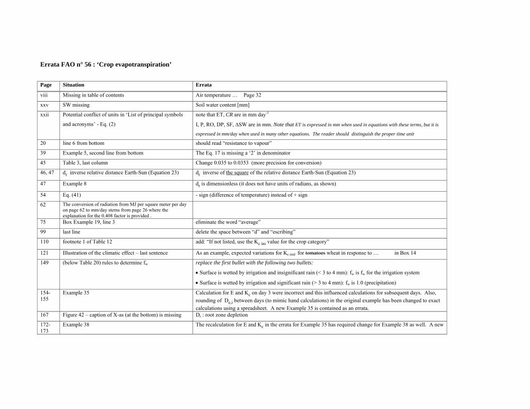
Errata FAO n° 56 : ‘Crop evapotranspiration’
Page Situation Errata
viii Missing in table of contents Air temperature … Page 32
xxv SW missing Soil water content [mm]
xxii Potential conflict of units in ‘List of principal symbols
and acronyms’ - Eq. (2)
note that ET, CR are in mm day-1
I, P, RO, DP, SF, ∆SW are in mm. Note that ET is expressed in mm when used in equations with these terms, but it is
expressed in mm/day when used in many other equations. The reader should distinguish the proper time unit
20 line 6 from bottom should read “resistance to vapour”
39 Example 5, second line from bottom The Eq. 17 is missing a ‘2’ in denominator
45 Table 3, last column Change 0.035 to 0.0353 (more precision for conversion)
46, 47 dr inverse relative distance Earth-Sun (Equation 23) dr inverse of the square of the relative distance Earth-Sun (Equation 23)
47 Example 8 dr is dimensionless (it does not have units of radians, as shown)
54 Eq. (41) - sign (difference of temperature) instead of + sign
62 The conversion of radiation from MJ per square meter per day on page 62 to mm/day stems from page 26 where the explanation for the 0.408 factor is provided .
75 Box Example 19, line 3 eliminate the word “average”
99 last line delete the space between “d” and “escribing”
110 footnote 1 of Table 12 add: “If not listed, use the Kc ini value for the crop category”
121 Illustration of the climatic effect – last sentence As an example, expected variations for Kc mid for tomatoes wheat in response to … in Box 14
149 (below Table 20) rules to determine fw replace the first bullet with the following two bullets:
• Surface is wetted by irrigation and insignificant rain (< 3 to 4 mm): fw is fw for the irrigation system
• Surface is wetted by irrigation and significant rain (> 3 to 4 mm): fw is 1.0 (precipitation)
154-155
Example 35 Calculation for E and Kc on day 3 were incorrect and this influenced calculations for subsequent days. Also, rounding of De,i between days (to mimic hand calculations) in the original example has been changed to exact calculations using a spreadsheet. A new Example 35 is contained as an errata.
167 Figure 42 – caption of X-as (at the bottom) is missing Dr : root zone depletion
172-173
Example 38 The recalculation for E and Kc in the errata for Example 35 has required change for Example 38 as well. A new
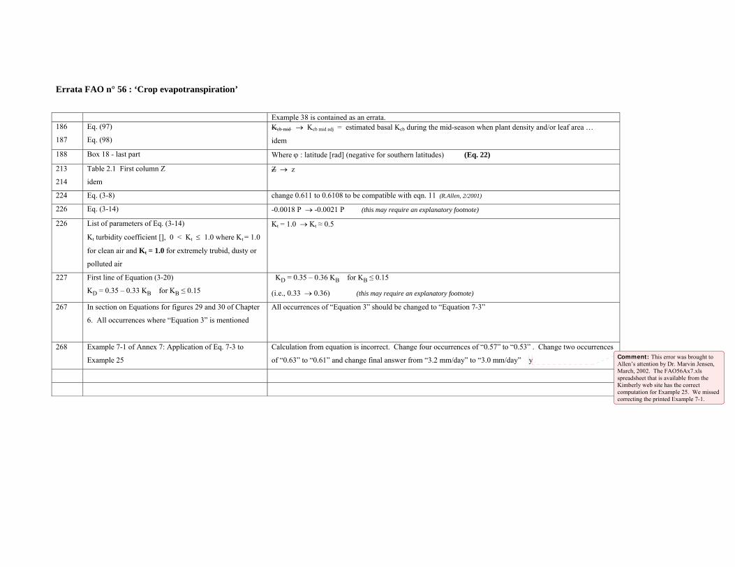
Errata FAO n° 56 : ‘Crop evapotranspiration’
Example 38 is contained as an errata. 186
187
Eq. (97)
Eq. (98)
Kcb mid → Kcb mid adj = estimated basal Kcb during the mid-season when plant density and/or leaf area …
idem
188 Box 18 - last part Where ϕ : latitude [rad] (negative for southern latitudes) (Eq. 22)
213
214
Table 2.1 First column Z
idem
Z → z
224 Eq. (3-8) change 0.611 to 0.6108 to be compatible with eqn. 11 (R.Allen, 2/2001)
226 Eq. (3-14) -0.0018 P → -0.0021 P (this may require an explanatory footnote)
226 List of parameters of Eq. (3-14)
Kt turbidity coefficient [], 0 < Kt ≤ 1.0 where Kt = 1.0
for clean air and Kt = 1.0 for extremely trubid, dusty or
polluted air
Kt = 1.0 → Kt ≈ 0.5
227 First line of Equation (3-20)
KD = 0.35 – 0.33 KB for KB ≤ 0.15
KD = 0.35 – 0.36 KB for KB ≤ 0.15
(i.e., 0.33 → 0.36) (this may require an explanatory footnote)
267 In section on Equations for figures 29 and 30 of Chapter
6. All occurrences where “Equation 3” is mentioned
All occurrences of “Equation 3” should be changed to “Equation 7-3”
268 Example 7-1 of Annex 7: Application of Eq. 7-3 to
Example 25
Calculation from equation is incorrect. Change four occurrences of “0.57” to “0.53” . Change two occurrences
of “0.63” to “0.61” and change final answer from “3.2 mm/day” to “3.0 mm/day” y
Comment: This error was brought to Allen’s attention by Dr. Marvin Jensen, March, 2002. The FAO56Ax7.xls spreadsheet that is available from the Kimberly web site has the correct computation for Example 25. We missed correcting the printed Example 7-1.
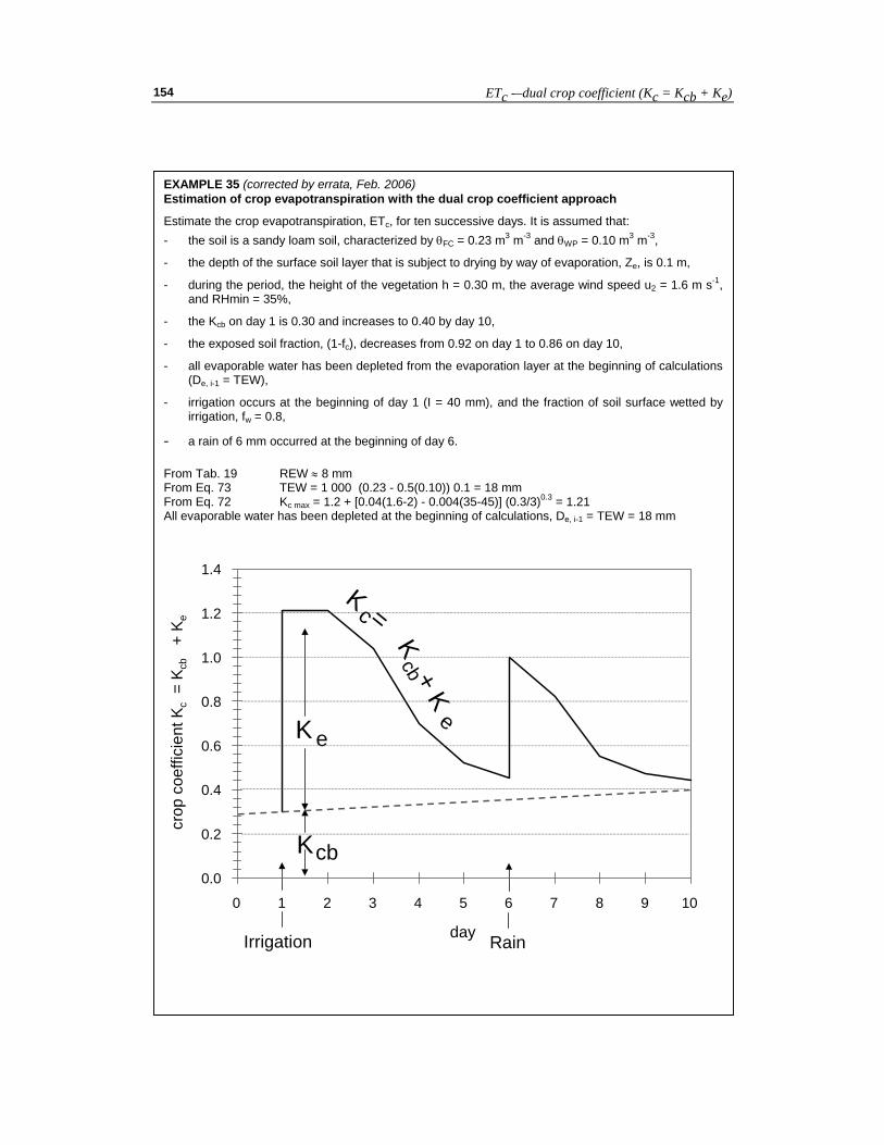
ETc -–dual crop coefficient (Kc = Kcb + Ke)
154
EXAMPLE 35 (corrected by errata, Feb. 2006) Estimation of crop evapotranspiration with the dual crop coefficient approach
Estimate the crop evapotranspiration, ETc, for ten successive days. It is assumed that: - the soil is a sandy loam soil, characterized by θFC = 0.23 m3 m-3 and θWP = 0.10 m3 m-3,
- the depth of the surface soil layer that is subject to drying by way of evaporation, Ze, is 0.1 m,
- during the period, the height of the vegetation h = 0.30 m, the average wind speed u2 = 1.6 m s-1, and RHmin = 35%,
- the Kcb on day 1 is 0.30 and increases to 0.40 by day 10,
- the exposed soil fraction, (1-fc), decreases from 0.92 on day 1 to 0.86 on day 10,
- all evaporable water has been depleted from the evaporation layer at the beginning of calculations (De, i-1 = TEW),
- irrigation occurs at the beginning of day 1 (I = 40 mm), and the fraction of soil surface wetted by irrigation, fw = 0.8,
- a rain of 6 mm occurred at the beginning of day 6. From Tab. 19 REW ≈ 8 mm From Eq. 73 TEW = 1 000 (0.23 - 0.5(0.10)) 0.1 = 18 mm From Eq. 72 Kc max = 1.2 + [0.04(1.6-2) - 0.004(35-45)] (0.3/3)0.3 = 1.21 All evaporable water has been depleted at the beginning of calculations, De, i-1 = TEW = 18 mm
K
K
e
cb
Irrigation Rain
K =c
cb
e
K + K
0.0
0.2
0.4
0.6
0.8
1.0
1.2
1.4
0 1 2 3 4 5 6 7 8 9 10
day
crop
coe
ffici
ent K
c =
K cb
+ K
e
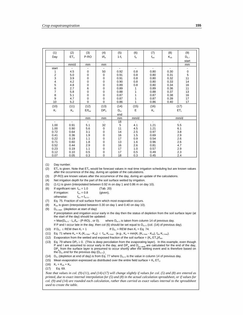
Crop evapotranspiration
155
(1) Day
(2) ETo
(3) P-RO
(4) I/fw
(5) 1-fc
(6) fw
(7) few
(8) Kcb
(9) De, i start
mm/d mm mm mm start 1 2 3 4 5 6 7 8 9 10
- 4.5 5.0 3.9 4.2 4.8 2.7 5.8 5.1 4.7 5.2
- 0 0 0 0 0 6 0 0 0 0
- 50 0 0 0 0 0 0 0 0 0
- 0.92 0.91 0.91 0.90 0.89 0.89 0.88 0.87 0.87 0.86
- 0.8 0.8 0.8 0.8 0.8 1 1 1 1 1
- 0.80 0.80 0.80 0.80 0.80 0.89 0.88 0.87 0.87 0.86
- 0.30 0.31 0.32 0.33 0.34 0.36 0.37 0.38 0.39 0.40
- 0 5 11 14 16 11 13 16 17 17
(10) Kr
(11) Ke
(12) E/few
(13) DPe
(14) De,i
end
(15) E
(16) Kc
(17) ETc
mm mm mm mm/d mm/d -
1.00 1.00 0.72 0.41 0.22 0.71 0.52 0.23 0.12 0.07
- 0.91 0.90 0.64 0.36 0.19 0.60 0.44 0.19 0.10 0.05
- 5.1 5.6 3.1 1.9 1.1 1.8 2.9 1.1 0.5 0.3
- 32 0 0 0 0 0 0 0 0 0
18 5 11 14 16 17 13 16 17 17 18
- 4.1 4.5 2.5 1.5 0.9 1.6 2.6 1.0 0.5 0.3
- 1.21 1.21 0.97 0.69 0.54 0.96 0.81 0.57 0.49 0.45
- 5.5 6.1 3.8 2.9 2.6 2.6 4.7 2.9 2.3 2.4
(1) Day number. (2) ETo is given. Note that ETo would be forecast values in real time irrigation scheduling but are known values
after the occurrence of the day, during an update of the calculations. (3) (P-RO) are known values after the occurrence of the day, during an update of the calculations. (4) Net irrigation depth for the part of the soil surface wetted by irrigation. (5) (1-fc) is given (interpolated between 0.92 m on day 1 and 0.86 m on day 10). (6) If significant rain: fw,i = 1.0 (Tab. 20) If irrigation: fw,i = 0.8 (given), otherwise: fw,i = fw,i-1. (7) Eq. 75. Fraction of soil surface from which most evaporation occurs. (8) Kcb is given (interpolated between 0.30 on day 1 and 0.40 on day 10). (9) De,i start (depletion at start of day) If precipitation and irrigation occur early in the day then the status of depletion from the soil surface layer (at
the start of the day) should be updated: = Max(De,i-1 - In,i/fwi - (P-RO)i , or 0). where De,i-1 is taken from column 14 of previous day. If P and I occur late in the day, then col (6) should be set equal to De,i-1 (col. (14) of previous day). (10) If De,i ≤ REW then Kr = 1 If De,i > REW then Kr = Eq. 74. (11) Eq. 71 where Ke = Kr (Kc max - Kcb) ≤ few Kc max. (e.g., Ke = min(Kr (Kc max - Kcb), few Kc max). (12) Evaporation from the wetted and exposed fraction of the soil surface = (Ke ETo)/few. (13) Eq. 79 where DPe ≥ 0. (This is deep percolation from the evaporating layer). In this example, even though
P and I are assumed to occur early in the day, and DPe and De,i end are calculated for the end of the day, DPe from the surface layer is presumed to occur shortly after the wetting event and is therefore based on the De,i.end for the previous day (De,I-1).
)
(14) De,i (depletion at end of day) is from Eq. 77 where De,i-1 is the value in column 14 of previous day. (15) Mean evaporation expressed as distributed over the entire field surface = Ke ETo. (16) Kc = Kcb + Ke. (17) Eq. 69. Note that values in col. (9)-(11), and (14)-(17) will change slightly if values for col. (5) and (8) are entered as printed, due to exact internal interpolation for (5) and (8) in the actual calculation spreadsheet, or if values for col. (9) and (14) are rounded each calculation, rather than carried as exact values internal to the spreadsheet used to create the table.
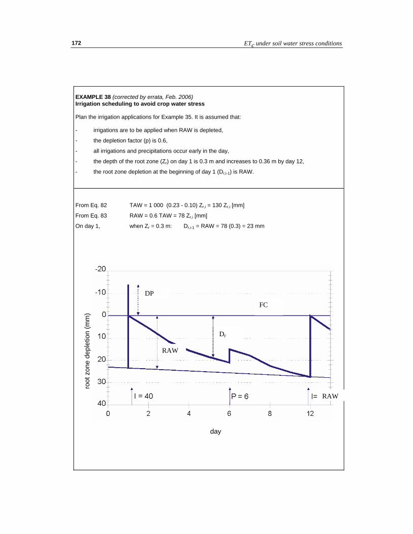
ETc under soil water stress conditions
172
EXAMPLE 38 (corrected by errata, Feb. 2006) Irrigation scheduling to avoid crop water stress Plan the irrigation applications for Example 35. It is assumed that: - irrigations are to be applied when RAW is depleted,
- the depletion factor (p) is 0.6,
- all irrigations and precipitations occur early in the day,
- the depth of the root zone (Zr) on day 1 is 0.3 m and increases to 0.36 m by day 12,
- the root zone depletion at the beginning of day 1 (Dr,i-1) is RAW. From Eq. 82 TAW = 1 000 (0.23 - 0.10) Zr,i = 130 Zr,i [mm]
From Eq. 83 RAW = 0.6 TAW = 78 Zr,i [mm]
On day 1, when Zr = 0.3 m: Dr,i-1 = RAW = 78 (0.3) = 23 mm
0 2 4 6 8 10
day
111 3 5 7 940
30
20
10
0
-10
-20
root
zon
e de
plet
ion
(mm
)
I = 40 I = RAWP = 6
RAW
DP
FC
Dr
RAW
RAW
DP
FC
Dr
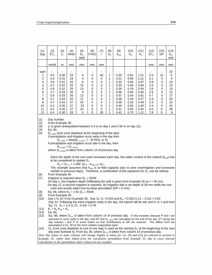
Crop evapotranspiration
173
(1) Day
(2) ETo
(3) Zr
(4)
RAW
(5) Dr,i
start
(6)
P-RO
(7) I
(8)Ks
(9) Kcb
(10) Ke
(11) Kc
(12) ETc
(13) DP
(14) Dr,i end
mm/d
m
mm
mm
mm
mm
mm
mm
mm
start 1 2 3 4 5 6 7 8 9 10 11 12
-
4.5 5.0 3.9 4.2 4.8 2.7 5.8 5.1 4.7 5.2 9.2 6.4
-
0.30 0.31 0.31 0.32 0.32 0.33 0.33 0.34 0.34 0.35 0.35 0.36
-
23 24 24 25 25 26 26 26 27 27 27 28
-
0 0 6 10 13 9 12 17 20 22 24 0
- 0 0 0 0 0 6 0 0 0 0 0 0
-
40 0 0 0 0 0 0 0 0 0 0
28
- 1 1 1 1 1 1 1 1 1 1 1 1
-
0.30 0.31 0.32 0.33 0.34 0.36 0.37 0.38 0.39 0.40 0.41 0.42
-
0.91 0.90 0.64 0.36 0.19 0.60 0.44 0.19 0.10 0.05 0.03 0.79
-
1.21 1.21 0.97 0.69 0.54 0.96 0.81 0.57 0.49 0.45 0.44 1.21
-
5.5 6.1 3.8 2.9 2.6 2.6 4.7 2.9 2.3 2.4 4.0 7.8
-
12 0 0 0 0 0 0 0 0 0 0 0
23 0 6 10 13 15 12 17 20 22 24 28 8
(1) Day number. (2) From Example 35. (3) Zr is given (interpolated between 0.3 m on day 1 and 0.36 m on day 12). (4) Eq. 83. (5) Dr,i start (root zone depletion at the beginning of the day) If precipitation and irrigation occur early in the day then Dr,i start = Max(Dr,i-1 end - I - (P-RO), or 0) If precipitation and irrigation occur late in the day, then Dr,i start = Dr,i-1end where Dr,i-1end is taken from column 14 of previous day Since the depth of the root zone increases each day, the water content of the subsoil (θsub) has
to be considered to update Dr,i Dr,i = Dr,i-1 + 1 000 (θFC - θsub,i-1) ∆Zr,I
The example assumes that θsub is at field capacity (due to prior overirrigation and excessive rainfall on previous days). Therefore, a combination of the equations for Dr,i can be utilized.
(6) From Example 35. (7) Irrigation is required when Dr,i ≥ RAW. On day 1, the irrigation depth (infiltrating the soil) is given from Example 35 as I = 40 mm. On day 12, a second irrigation is required. An irrigation with a net depth of 28 mm refills the root
zone and avoids water loss by deep percolation (DP = 0 mm). (8) Eq. 84, where Ks = 1 for Dr,i ≤ RAW. (9) From Example 35. (10) Day 1 to 10: From Example 35. Day 11: Kr =0.033 and Ke = 0.033 (1.21 – 0.41) = 0.03
Day 12: Following the extra irrigation early in the day, the topsoil will be wet and Kr is 1 and from Eq. 71: Ke = 1.0 (1.21 - 0.42) = 0.79.
(11) Kc = Ks Kcb + Ke. (12) Eq. 80. (13) Eq. 88, where Dr,i-1 is taken from column 14 of previous day. In this example, because P and I are
assumed to occur early in the day, and DP and Dr,i end are calculated for the end of the day, ET during the day reduces I and P to some extent so that contributions to DP are reduced. This differs from the assumption in Ex. 35 for the more shallow evaporation layer.
(14) Dr,i (root zone depletion at end of one day) is used as the starting Dr,i at the beginning of the next day (see footnote 5). From Eq. 85, where Dr,i-1 is taken from column 14 of previous day.
Note that values in some columns will change slightly if values for col. (9) and (10) are entered as printed in Example 35, rather than linked from the calculation spreadsheet from Example 35, due to exact internal calculations in the spreadsheet where values are not rounded.

ETc under soil water stress conditions
174