failure of anisotropic shales under triaxial stress conditions · failure of anisotropic shales...
TRANSCRIPT

1
Imperial College London
Department of Earth Science and Engineering
Failure of Anisotropic Shales under
Triaxial Stress Conditions
by
Jasmin Ambrose
A thesis submitted in fulfilment of the requirements for the degree
of Doctor of Philosophy and the Diploma of Imperial College
June 2014

2
Copyright
The copyright of this thesis rests with the author and is made available under a Creative
Commons Attribution-Non Commercial-No Derivatives licence. Researchers are free to copy,
distribute or transmit the thesis on the condition that they attribute it, that they do not use
it for commercial purposes and that they do not alter, transform or build upon it. For any
reuse or distribution, researchers must make clear to others the licence terms of this work.
Declaration
I hereby declare that this thesis, entitled “Failure of Anisotropic Shales under Triaxial Stress
Conditions”, is entirely my own work. All materials created by others that are used in the
thesis have been given full acknowledgement.

3
Abstract
Shales are highly anisotropic in their mechanical behaviour. The strength of anisotropic
shales depends not only on the magnitude of the principal stresses, but also on the bedding
plane orientations relative to the principal stresses. In this study, the failure of shales are
investigated using triaxial compression and extension tests, while the role of intermediate
stress (2) on the strength of anisotropic shale is evaluated using data from new triaxial
extension tests, as well as data from the literature.
Triaxial compression and extension experiments were made on two organic-rich shales, at
different confining stresses and bedding angles (). Examination of post-failure computed
tomography (CT) and thin section images for high strength anisotropy shale show that, for
large and small values of , the fracture plane follows the angle that is predicted by the
Coulomb’s failure criterion for an isotropic material. In the range of angles of roughly
35o<<75o, failure occurs along the bedding plane. Both of these results are consistent with
the assumptions of Jaeger’s plane of weakness (JPW) model. However, there exists a
transition regime of loading angles lying between about 10o and 35o, wherein the failure
surface follows an irregular path that may jump between the bedding plane and the plane
defined by the Coulomb criterion. In this regime, the strength of the rock is lower than the
strength predicted by JPW model. For the shale with low strength anisotropy, the failure
plane angles agree with the predictions of JPW model.
The triaxial compression experimental data on shales and several data sets from the
literature were fit with both Pariseau’s continuum model for the failure of transversely
isotropic materials and JPW model. Comparison of both models show that the Pariseau
model provided a better fit for ten of the twelve rocks, whereas the JPW model provided a
better fit only for two low strength anisotropy shales. It was noted that all the rocks with a
strength anisotropy ratio (SAR) > 2 were fit more closely by the Pariseau model, whereas
both shales that were a better fit with the JPW model had SAR < 2. Pariseau’s model is also
more robust and accurate than Jaeger’s model when using a reduced numbers of data (i.e.,
data collected at fewer confining stresses and/or fewer angles).
Finally, both the JPW model and Pariseau’s model was applied in the true-triaxial stress
regime, in which 1 >2 > 3. When analysed with Mogi’s experimental data on Chichibu
Schist, both models could predict failure under true-triaxial stress conditions. Mogi’s data
and the triaxial extension experiments for the two shales shows that an increase in the
intermediate stress 2 increases the intact rock strength, whereas weak plane failure
depends not only on intermediate stress 2, but also on bedding plane angle and foliation
direction ().

4
Acknowledgements
I would like to thank Prof. Zimmerman for having faith in me and for being a great mentor
and teacher. His smart suggestions and guidance was crucial to the success of this project.
Special thanks also to Roberto Suarez-Rivera and Sidney Green for giving me the
opportunity to work on this research project at Schlumberger TerraTek in Salt Lake City,
Utah. This experience gave me good exposure on rock mechanics, petrology and shales.
The excellent experimental results in this project would not have been possible if not for the
highly experienced, professional and dedicated staff at TerraTek such as Cecil, Aaron, Nancy,
Jim, Sanket, Kevin, Lorenzo, Rex, Jed, Chai, Ed and many others that have been involved
throughout the various stages of this project.
I would also like to thank my friends and colleagues at Schlumberger TerraTek and the
Innovation Center including Roberto Castaneda, Chon La, Julia, Eric Edelman, Maxim,
Alexandra, Sergey, Dean, Neil, Ryan, Megan, Doug, Iranga, Rahul, Red, Jeff, Aniket and Jun
Le. Your friendship made this a memorable journey. Special thanks also to Patrick, Tina and
John for their contributions on the petrology work.
At Imperial College, I would like to thank Ali, Gaurav, Kamal and Dave for their friendship
throughout this journey. I am lucky to have such thoughtful friends.
This study would not have been possible without the support and encouragements of my
family. Sincerest gratitude to Amma, Appa, Jerome, Angie, Auntie, Parti, Ramesh and family
members who supported and consoled me throughout.
To Abhe, Gabriel and Trinity, I will never be able to repay your patience and understanding
for moving with me three times from the start of this research project, beginning from
Mexico, then Colombia, and later to Salt Lake City. I look forward to our future adventures
together.
Lastly, I would like to thank Schlumberger for funding and supporting me throughout this
research project.

5
Contents Chapter 1 Introduction
1.1 Importance of understanding the strength of shale formations…………………………….. 8
1.2 Application of failure criteria in shale formations………………………………………............. 10
Chapter 2 Review of Rock Failure Criteria
2.1 Classification of failure criteria………………………………………………………………………………. 13
2.2 Review of failure criteria of anisotropic rocks………………………………………………………… 15
2.3 Jaeger’s Plane of Weakness Model (JPW)…………………………………………………............... 16
2.4 Jaeger’s continuously varying shear stress model………………………………….................. 17
2.5 McLamore and Gray model………………………………………………………………….................... 18
2.6 Walsh and Brace model…………………………………………………………………………………………. 19
2.7 Ramamurthy model…………………………………………………………………………………............... 20
2.8 Pariseau’s model……………………………………………………………………………………………………. 21 2.9 Review of other anisotropic failure criteria……………………………………………………………. 22 2.10 Influence of intermediate stress in anisotropic rocks…………………………………………… 23
Chapter 3 Laboratory Experiments
3.1 Introduction…………………………………………………………………………………………………………… 26
3.2 Bossier shale description……………………………………………………………………………………….. 28
3.3 Vaca Muerta shale description………………………………………………………………………………. 29
3.4 Sample preparations and quality control……………………………………………………………….. 31
3.5 Triaxial compression and extension setup……………………………………………………………… 32
3.6 Measurements and experimental results………………………………………………………………. 33
3.6.1 Strength of Bossier shale and Vaca Muerta shale……………………………………. 36
3.6.2 Elastic moduli of Bossier shale and Vaca Muerta shale………………………….... 42
Chapter 4 Fabric Analysis
4.1 Petrology……………………………………………………………………………………………………………….. 47
4.2 CT Scan (Pre-test and Post-test) of Bossier shale and Vaca Muerta shale samples…. 49
4.3 Thin section analysis………………………………………………………………………………………………. 58
Chapter 5 Jaeger Plane of Weakness (JPW) Model
5.1 Theory and data-fitting technique…………………………………………………………………………. 62
5.2 Jaeger plane of weakness model applied to data…………………………………………………… 70
5.2.1 Bossier shale data analyzed using the JPW model……………………………………. 75
5.2.2 Vaca Muerta shale data analyzed using the JPW model…………………………… 76
5.3 JPW Strength anisotropic ratio (SAR)……………………………………………………………………… 77
5.4 JPW model applied to triaxial extension………………………………………………………………… 80

6
5.5 JPW model applied to data from literature……………………………………………………………. 86
5.6 JPW model using reduced numbers of data sets……………………………………………………. 89
Chapter 6 Pariseau’s Model
6.1 Theory and data-fitting technique…………………………………………………………………………. 92
6.2 Pariseau model applied to data……………………………………………………………………………… 96
6.2.1 Bossier shale data analyzed using Pariseau’s model………………………………… 97
6.2.2 Vaca Muerta shale data analyzed using Pariseau’s model……………………….. 99
6.3 Pariseau Strength Anisotropy Ratio (SAR)………………………………………………………………. 100
6.4 Pariseau’s model applied to triaxial extension……………………………………………………….. 101
6.5 Pariseau’s model applied to data from literature…………………………………………………… 103
6.6 Pariseau model using reduced numbers of data sets……………………………………………... 106
6.7 Pariseau model sensitivity analysis………………………………………………………………………… 107
Chapter 7 Failure of Anisotropic Rocks under True-Triaxial Conditions
7.0 Introduction…………………………………………………………………………………………………………… 110
7.1 JPW model under true-triaxial conditions………………………………………………………………. 111
7.2 Pariseau model under true-triaxial conditions……………………………………………………….. 114
7.3 Mogi Chichibu Schist true-triaxial experiments………………………………………………………. 117
7.4 JPW model validation using true-triaxial Mogi Chichibu Schist data………………………. 120
7.5 Comparison of JPW model using conventional triaxial against true-triaxial data……. 125
7.6 Pariseau model validation using true-triaxial Mogi Chichibu Schist data………………… 128
7.7 Bossier shale calibration of JPW and Pariseau models using compression and
extension data ………………………………………………………………………………..........................
130
7.8 Vaca Muerta shale calibration of JPW and Pariseau models using compression and
extension data………………………………………………………………………………………………………..
133
Chapter 8 Summary, Conclusions and Recommendations
8.1 Summary and conclusions……………………………………………………………………………………… 136
8.2 Recommendations…………………………………………………………………………………………………. 141
References…………………………………………………………………………………………………………………… 144
Appendix A Laboratory triaxial compression and extension data
Appendix A1. Bossier shale experimental data……………………………………………….. 153
Appendix A2. Vaca Muerta shale experimental data………………………………………. 195
Appendix B Matlab codes
Appendix B1. JPW model objective function…………………………………………………… 219
Appendix B2. JPW model main loop………………………………………………………………… 222
Appendix B3. Pariseau model objective function……………………………………………. 223

7
Appendix B4. Pariseau model main loop…………………………………………………………. 225
Appendix B5. True-triaxial Pariseau model objective function……………………….. 226
Appendix B6. True-triaxial Pariseau model main loop…………………………………….. 229
Appendix B7. True-triaxial Pariseau model strength 1 prediction…………………. 231
Appendix B8. True-triaxial JPW model strength 1 prediction………………………… 233
Appendix C Differentiate Coulomb criterion for min……….………………………………………… 234
Appendix D Data from literature
Appendix D1. Data from literature – various anisotropic rocks………………………. 236
Appendix D2. Data from literature – Chichibu Schist (Mogi, 1979 and 2007)…. 238
Appendix E JPW model analysis for various anisotropic rocks…………………………………… 239
Appendix F Pariseau model analysis for various anisotropic rocks……………………………. 252
Appendix G Example of Pariseau model iteration……………………………………………………… 265

8
1 Introduction
1.1 Importance of understanding the strength of shale formations
Jaeger (1962) described rock mechanics as a “new engineering subject” in his monograph
“Elasticity, Flow and Fracture”. In the same year, Leopold Muller founded the ISRM with his
motivation encapsulated by the comment “We don’t know the rock mass strength. That is
why we need an International Society” (Hudson, 2008). During these times, rock mechanics
was just starting to be recognized as a discipline worthy of a special course of lectures in an
engineering program. Nowadays, rock mechanics is no longer described as a new subject,
but the importance of predicting rock strength remains the same, but with more emphasis
of increased appreciation of its anisotropic nature.
Isotropic intact rocks are relatively easy to test or interpret, and much is already understood
regarding their behavior. However, predicting and modeling the strength of anisotropic
rocks is one of the most important unsolved problems in rock mechanics (Hudson, 2008).
Such solutions are valuable for finding answers for well construction or geomechanics
applications, whereby failure of rock around the boundary of an excavation depends on the
stress concentration around the opening and strength in different directions. Al-Ajmi (2006)
and Zimmerman (2010) demonstrated the importance of incorporating the effect of the
intermediate stress into wellbore stability analysis for isotropic rocks. However, the
application of true-triaxial failure criteria for well construction was made only after many
years of research on isotropic rocks. Now, with the present shift of the world energy market
towards shale gas, it is natural that more studies are made to understand the anisotropic
behavior of shales before applied for well construction in shale formations. This is
important, because isotropic criteria should not be used for predicting the strength of
anisotropic shales, as the strength of highly anisotropic shales can sometimes be ten times
lower that its maximum strength, depending on the angle between the bedding plane and
the direction of the maximum principal stress.
Tight shales are typically characterized by dominant matrix mineral composition, organic
content and maturation, porosity and pore fluid saturation (Suarez-Rivera and Fjaer, 2012).
However, for rock mechanics applications, it is more useful to think of shales in terms of
their mineral and organic content. Goodman (1989) recognized the need for a behavior-
based classification for rock mechanics analysis instead of the origin-based classification
(i.e., metamorphic, sedimentary and igneous) and classified rocks as crystalline, clastic, fine-
grained and organic. Within the fine-grained rocks, shales can be further sub-classified
based on the degree of anisotropy and strength category. Organic-rich shales fall under the
category of organic rocks. These classifications, although somewhat descriptive, are still too
general and do not give a definition that can be standardized for organic-rich shales.

9
In this study, shale is described using the “mental picture” proposed in Figure 1.1. The
mechanical behavior of shales is strongly influenced by three factors: its natural
discontinuities, its texture, and its composition. The left-hand column of the mental picture
in Figure 1.1 shows how the scale of the discontinuities, which represents the length, width
and frequency of the discontinuities, relate to the overall mechanical behavior. When these
discontinuities are weaker than the matrix rock, they are called “planes of weakness”, which
result in strength anisotropy. Unlike for the case of isotropic rocks, anisotropic shales need
to be analyzed down to finer m scales, as shown by the thin section image in Figure 1.1. At
this scale, lamination and bedding plane features that contribute to the mechanical
behavior become relevant.
Figure 1.1. “Mental picture” of shales showing weak planes, texture and composition.
Shales are, strictly by definition, fissile rocks, but the industry usage of the term shale is
broad and usually refers to the fine matrix rock. “Matrix rock” normally denotes rock having
particles that are not distinguishable by the naked eye, while “sand” and “silt” generally
refer to rock whose particles can be seen and are distinct. Using this broad definition, most
shales can be categorized into calcite-rich, quartz-rich, or clay-rich. The texture of the shales
will depend on the arrangement of mineral components within the matrix rock, resulting in

10
heterogeneity. An example of highly laminated shale is shown in the middle column of
Figure 1.1, by a sample picture and a thin section image. The fine scale shown in the thin
section image needs to be considered in order to distinguish different shale behaviors.
Taking a closer look at the shale fabric, the mechanical behavior of a shale can be described
by its texture and composition. The shale diagram shown on the right hand column of Figure
1.1 describes this textural and compositional effect, categorized by its mineral composition.
For the calcite rich shales, shale types with the same composition but with different textural
effect (i.e., lumped vs. dispersed calcite), results in a wackestone or carbonate mudstone.
Similarly, for the case of quartz shales, the arrangement of the quartz mineral within the
shale matrix results in a silty mudstone or siliceous mudstone. Lastly, for clay-rich shales,
high lamination or bioturbation would result in laminated claystone or bioturbiditic
claystone. The presence of other material such as fossils, minerals, organics, and fluid within
the shale matrix or laminations further alters and influences its mechanical behavior.
1.2 Application of failure criteria in shale formations
One of the most important applications of rock mechanics to petroleum engineering is the
problem of wellbore stability (Zimmerman, 2010). Although the focus of this study is not on
wellbore stability, there is an urgent need for an anisotropic failure criterion for the
improved design of wellbores in shale formations. Apart from wellbore stability analysis,
shale strength is also important in mining and in civil engineering (e.g., tunneling, bored
piles, etc.) where shale strength anisotropy can have a large impact (Ewy et al., 2010).
However, as the focus of this study is on reservoir shales, the discussion here is mostly
aimed at application for wellbore stability analysis.
Wellbore stability analysis is usually conducted using isotropic models such as Mohr-
Coulomb, Drucker-Prager, Von Mises, Modified Lade or Hoek-Brown (Han and Meng, 2014).
Although isotropic models have been used for many years in the oil and gas industry,
application of these models is severely limited in shale formations, as the strength of
anisotropic shales are often overestimated and may lead to stability problems. To highlight
the fact that shales are highly anisotropic, Ewy et al. (2010) tested six types of claystones,
and found reduced strength along the weak plane by 10-70% for cohesion, and by 7-17% for
friction angle.
To incorporate the effect of intermediate stress 2 on the strength of isotropic rocks, Al-
Ajmi and Zimmerman (2005) developed the Mogi-Coulomb failure criterion that accounts
for 2, and showed that this criterion was better at predicting the strength of a variety of
isotropic rocks. Al-Ajmi and Zimmerman (2006), using data from the literature, applied their
earlier findings on Mogi-Coulomb to wellbore stability analysis. Their main finding shows
that the Drucker-Prager criterion overestimates wellbore strength, and the Mohr-Coulomb

11
criterion underestimates wellbore strength, whereas the Mogi-Coulomb criterion predicts
wellbore strength reasonably well.
For anisotropic rocks, similar wellbore stability analyses were made for conventional triaxial
stress conditions (1 > 2 = 3) by various researchers. Wong et al. (1993) correlated shale
strength and sonic measurements from the North Sea, and presented an approach to
optimize shale formation drilling for high angle wells, suggesting practical methods to avoid
stuck pipe situations. Santarelli et al. (1997) also suggested procedures to optimize drilling in
shales and described that wellbore stability problems result in 10% to 15% of drilling cost,
where a significant number of these issues are due to shale instability. Aadnoy et al. (1988)
made one of the earliest evaluations of the plane of weakness criterion for wellbore stability
analysis, and showed that ignoring strength anisotropy leads to erroneous wellbore strength
predictions. Aadnoy et al. (2009) later applied the plane of weakness criterion for wellbores
in Canada, which led to the successful completion of wells that previously had significant
shales instability issues.
Wu and Tan (2010) used experimental data from Bohai Bay, China, and data sets from the
literature, to evaluate the plane of weakness model for highly anisotropic shales, and
applied this strength model for wellbore stability analysis. Their main finding suggests that
shale strength anisotropy mainly affects high angle and horizontal wells. Narayanasamy et
al. (2009) analyzed wells from the UK Continental Shelf that presented instabilities in the
unstable Cretaceous mudstone. To overcome these shale instabilities, cores were taken
from the shale formation and tested to determine its strength properties, and applying the
plane of weakness model to design and complete the well successfully. Lee et al. (2012a)
used the plane of weakness criterion to determine that the wellbore strength for anisotropic
shales is significantly affected by the well orientation and in-situ stress field.
Past works on wellbore stability for anisotropic shales were mostly done using isotropic rock
criteria, or the plane of weakness criterion. The former criteria should not be used for shales
as it overestimates strength, whereas for the latter, no validation was made to determine
how the plane of weakness criterion compares to other anisotropic rock models.
Furthermore, there is also a lack of understanding of the role of the 2 effect for anisotropic
rocks, which could significantly underestimate strength. Therefore, there is room for
improving or validating existing anisotropic rock strength models, and testing their
capabilities in the true-triaxial stress regime. In the following chapters, the experiments
made on shales and the true-triaxial model described attempt to demonstrate a clear
method and approach for using anisotropic models for predicting strength of anisotropic
shales. The failure criteria used and validated in this study for anisotropic rocks is applicable
for wellbore stability, or other civil engineering and construction applications.
The next chapter describes the various anisotropic rock failure criteria that are available in
the literature. This is followed by details of the laboratory measurements on two types of
shales made in this study. From the various anisotropic rock failure criteria, the Jaeger plane

12
of weakness (JPW) failure criterion and the Pariseau failure criterion will be described in
detail. The JPW and Pariseau failure criteria will then be evaluated using data from the
laboratory experiments and the literature. Lastly, the validity of these two criteria will be
investigated under true-triaxial stress conditions using data from the literature and the
experimental data from this study.

13
2 Review of Rock Failure Criteria
2.1 Classification of failure criteria
A “failure criterion” is an equation that defines, either implicitly or explicitly, the value of the
maximum principal stress that will be necessary in order to cause the rock to “fail”, which in
the case of brittle behavior can be interpreted as causing the rock to break along one or
more “failure planes”. Rock failure criteria can be classified as isotropic or anisotropic,
depending on whether or not they are intended to apply to rocks that exhibit anisotropic
behavior. Pariseau (2012a, 2012b), Lade (1993) and Brady and Brown (1993) provided
reviews of those failure criteria for isotropic rocks that are most commonly used in practice.
For anisotropic rocks, Duveau et al. (1998) classified failure criteria as either continuous or
discontinuous, depending on whether or not they were expressed in terms of a single
mathematical equation, or two or more equations that apply in different stress regimes.
Within the continuous criteria, they were further categorized as mathematical, or empirical.
The Duveau et al. classification presented in Table 2.1 has been augmented with additional
criteria uncovered during the present study.
An additional categorization can be made regarding whether or not the criterion accounts
for the possibility that all three principal stresses may be unequal. Those criteria that do
attempt to account for the influence of the intermediate principal stress, referred to
hereinafter as being “true-triaxial criteria”, are identified with an asterisk.
Almost half of the criteria presented in Table 2.1 are “mathematical”, and in this approach,
the rock is treated as a solid body with properties that vary continuously with direction. The
usual features of these mathematical models are that the issues of orientation (bedding
angle , and foliation direction ) are accounted for, while parameters such as friction angle
and cohesion are not explicitly required. Strictly speaking, these latter two parameters are
necessary only in a Coulomb criterion. Most of these mathematical models have not yet
been widely used in engineering practice – perhaps due to mathematical complexity, and
perhaps also due to lack of experimental validation (e.g., Cazacu and Cristescu, 1999;
Kusabuka et al., 1999; Lee and Pietruszczak, 2007; Mroz and Maciejewski, 2011). For
anisotropic rocks, perhaps the most commonly used mathematical model is the Pariseau
(1968) criterion.
The criteria that are classified as using the “empirical approach” are mainly extensions of
the Coulomb or Von Mises isotropic criteria and do not use bedding angle or foliation
direction. Instead, the various parameters are determined from fitting experimental data.
Parameters determined from this approach are orientation specific, although orientation is
not part of the equations defining the parameters. Sheorey (1997) conducted an extensive

14
review of those empirical rock failure criteria for isotropic and anisotropic rocks that are
most common in the construction industry. This approach is easily developed or modified
from existing failure criteria. Some of the latest empirical approaches proposed are
extensions of the Hoek-Brown isotropic rock failure criterion adapted to true-triaxial
conditions (e.g., Saroglou and Tsiambaos, 2007a; Zhang & Zhu 2007; Lee et al., 2012). This
approach is not based on any physical or mathematical foundation, and been criticized for
this reason (Duveau et al., 1998).
Table 2.1. Classification of anisotropic failure criteria; updated from Duveau et al. (1998).
Continuous criteria Discontinuous criteria
Mathematical approach Empirical approach Von Mises (1928)* Casagrande and Carrillo (1944) Jaeger (1960, 1964*)
Hill (1948)* Jaeger variable shear (1960) Walsh and Brace (1964)
Olszak and Urbanowicz (1956) McLamore and Gray (1967) Hoek (1964, 1983)
Goldenblat (1962) Ramamurthy, Rao and Singh (1988) Murrell (1965)
Goldenblat and Kopnov (1966) Ashour (1988)* Barron (1971)
Boehler and Sawczuk (1970, 1977) Zhao, Liu and Qi (1992) Ladanyi and Archambault (1972)
Tsai and Wu (1971)* Singh, et al. (1998)* Bieniawski (1974)
Pariseau (1968)* Tien & Kuo (2001) Hoek and Brown (1980)
Boehler (1975) Tien, Kuo and Juang (2006) Smith and Cheatham (1980a)*
Dafalias (1979, 1987) Tiwari and Rao (2007)* Yoshinaka & Yamabe (1981)*
Allirot and Boehler (1979) Saroglou and Tsiambaos (2007a) Duveau and Henry (1997)
Nova and Sacchi (1979)* Zhang & Zhu (2007)* Pei (2008 )*
Nova (1980, 1986)* Lee, Pietruszczak and Choi (2012)* Zhang (2009)*
Boehler and Raclin (1982)
Raclin (1984)
Kaar et al. (1989)
Cazacu (1995)
Cazacu and Cristescu (1999)*
Kusabuka, Takeda and Kojo (1999)*
Pietruszczak and Mroz (2001)*
Lee and Pietruszczak (2007)*
Mroz and Maciejewski (2011)*
Bold – Criteria added since Duveau et al. (1998)
* – True-triaxial criteria
The discontinuous criteria are generally related to the Coulomb criterion (i.e., Jaeger, 1960).
In these criteria, the failure mechanisms that occur along the weak planes or intact rock are
distinguished. The assumption is that the rock fails either through shear fracture or sliding
along weak planes. These two failure modes are used together to determine the actual
failure criterion. Most of the criteria within this category are easily used for design
applications, because they are based on the Coulomb strength parameters. However, some
of the discontinuous criteria use an empirical approach (Hoek et al., 1992) or mathematical

15
models (Pei, 2008) to account for failure along weak planes. Duveau and Henry (Duveau et
al., 1998) combined Lade’s true-triaxial criteria for isotropic rocks with Barton’s criterion
(Barton and Choubey, 1977) for anisotropic rocks. The relative ease of modifying and
combining two criteria for isotropic and anisotropic rocks led to these various other
combinations for the discontinuous model.
2.2 Review of failure criteria of anisotropic rocks
Although failure criteria for anisotropic rocks have not received nearly as much study as has
the topic of failure criteria for isotropic rocks, nevertheless a literature review reveals
several studies of the strength of anisotropic rocks. Among the pioneering and most well
known approaches are Jaeger’s (Jaeger, 1960) “Plane of Weakness” model, denoted
hereafter as JPW, and Jaeger’s variable shear strength model (Jaeger, 1964). To date, the
JPW criterion seems to be the most widely used for predicting anisotropic rock strength.
Donath (1961) was the first to evaluate the applicability of Jaeger’s theory for Martinsburg
slate. Chenevert and Gatlin (1964) also analyzed the Martinsburg slates to confirm Jaeger’s
criterion, and observed that this rock’s elastic moduli are transversely isotropic. McLamore
and Gray (1967) then extended Jaeger’s variable shear strength model by varying the
friction angle, and applied this model to the Green River shale. In the same study,
McLamore and Gray also presented evidence that the Walsh and Brace (1964) model is
identical to the JPW because both models are derived from the same criteria.
Other notable early experimental works include the yielding of soft diatomite rocks under
hydrostatic pressure (Allirot et al., 1977), revealing critical anisotropic properties supported
by images of sample deformation. This study displayed evidence of a non-shear type failure
for anisotropic rocks. This is uncommon, as most rocks fail in shear under compressive load.
Another important research work was that of Attewell and Sandford (1974), who observe
reduced anisotropy of the Penrhyn slate with increased stress. The phenomenon of reducing
anisotropy was also reported by Ramamurthy et al. (1993), based on extensive experiments
on the Himalayan schist, leading to development of an empirical failure criterion.
Since the role of 2 in the failure of isotropic rocks was recognized, various researchers
extended this concept to anisotropic rocks, with limited success (e.g., Tiwari & Rao, 2007;
Singh et al., 1998; Zhang and Zhu, 2007). While most research on strength anisotropy
assumed conventional triaxial conditions, Jaeger (1964) and Pariseau (1968) extended
strength anisotropy to account for the 2 effect. Jaeger introduced the first anisotropic rock
failure criterion that includes 2, and discussed some of the results from his experimental
work in his review of Donath’s work (Donath, 1964, p. 298).
Pariseau (1968) modified Hill’s theory for metal anisotropy (Hill, 1948), obtaining a failure
criterion that incorporates the effect of 2. Although Duveau et al. (1998) validated

16
Pariseau’s model for the Angers schist, both Jaeger and Pariseau’s model were never
validated using true-triaxial experimental data. The true-triaxial Pariseau model has
similarities with the Drucker-Prager (1952) model for isotropic rocks, as several researchers
have demonstrated (Tsai and Wu, 1971; Smith and Cheatham, 1980b; Kusabuka et al.,
1999). Ong and Roegiers (1993), using Pariseau’s model, showed that high strength
anisotropy significantly influences the stability of horizontal wells. A similar study of
wellbore stability by Suarez-Rivera et al. (2009) showed that the Pariseau strength model,
combined with an anisotropic elastic rock model, provides more conservative results than
are obtained by using the JPW strength model in combination with an isotropic elastic
model.
In the next sections, several failure criteria commonly known in the petroleum industry are
described and presented in units of psi. Similarly, all data in this study will be presented in
units of psi, to maintain consistency.
2.3 Jaeger’s Plane of Weakness Model (JPW)
The Coulomb, or the linear Mohr criterion, is sometimes referred to as the Mohr-Coulomb
criterion. In 1773 Coulomb, based on experimental evidence, proposed that failure of
geomaterials occurs along a plane when the shear stress acting along that plane reaches a
critical value that is able to overcome a “frictional” type resistance force, plus an additional
“cohesive” force (Jaeger et al., 2007). This condition for failure is
| | . (2.3.1)
The shear stress and normal stress , on a plane at angle to the direction of 1, defined
as shown in Figure 2.1. The definition for angle described in Figure 2.1 is provided for
clarity, whereas the remainder of this study uses the standard convention that is presented
and used from Chapter 3 onwards.
Figure 2.1. Triaxial compression test setup for sample angle .

17
For the angle defined in Figure 2.1, shear and normal stress n expressed in terms of
maximum shear stress, m = (1-3)/2, and mean normal stress, m = (1+3)/2, are given by
, (2.3.2)
, (2.3.3)
where 1 and 3 are the major and minor principal stresses. Jaeger (1960) extended the
Coulomb criterion to the idealized model of a rock that contains a preexisting plane that is
weaker than the intact rock. This JPW criterion, expressed in terms m and m (found by
inserting Eqn. 2.3.2 and Eqn. 2.3.3 into Eqn. 2.3.1), is
(
) [ (
)]. (2.3.4)
For intact rock failure with cohesion So and friction angle o, there will be a critical plane at
angle where the shear strength will be first reached as 1 is increased (Brady and Brown,
1993; p. 107; Parry, 2000). For intact rock this occurs at an angle of = 45 - o/2 (Jaeger et
al., 2007; p. 91) where is defined clockwise on the Mohr circle. Inserting the fracture angle
= 45 - o/2 into Eqn. 2.3.4 results in the isotropic rock Coulomb failure criterion:
. (2.3.5)
The JPW criterion for failure along the weak plane is defined by Eqn. 2.3.4, and for failure of
intact rock is defined by Eqn. 2.3.5. These two equations form the foundation of the various
other criteria described in Table 2.1. Chapter 5 of this study gives a detailed explanation of
the derivation and analysis of this criterion.
2.4 Jaeger’s continuously varying shear stress model
From the Coulomb criterion, Jaeger (1960) derived another approach based on the concept
of “varying shear strength”. This method assumes that the cohesion of the rock, S, changes
with bedding angle , while the friction coefficient tan is constant, where S1 and S2 are
parameters, and the shear strength of the rock varies between S1 - S2 and S1 + S2:
( ), (2.4.1)
and where is the critical plane at angle where the shear strength will be first reached as
1 is increased. For failure in a uniform medium with shear strength S and friction
coefficient tan , it is found from substituting Eqn. 2.3.2 and 2.3.3 into Eqn. 2.3.1 that S has a
maximum value when = 45 - /2 (Jaeger, 1960). By assuming that 0 < < /2 and 0 < <
/2, and inserting Eqns. 2.3.2, 2.3.3 and 2.4.1 into the Coulomb criterion (Eqn. 2.3.1), the
varying shear stress criterion can be written in terms of m and m as

18
( ) ( ) . (2.4.2)
The parameters S1 and S2 are determined by fitting data to Eqn. 2.4.1, where cohesion S is
determined by the intercept on the Mohr circle. McLamore and Gray (1967) tested this
approach, and concluded that Eqn. 2.4.1 does not describe the actual variation of S over the
entire range of angles . To overcome this problem, they proposed an improvement, by
assuming that the friction angle also varies with angle , similar to Jaeger’s varying cohesion
model.
2.5 McLamore and Gray model
McLamore and Gray (1967) modified Jaeger’s variable shear strength approach by proposing
that cohesion S and the angle of internal friction both vary with bedding angle .
McLamore and Gray’s varying S and equations are
( ) , (2.5.1)
( ) , (2.5.2)
The parameters A, B, C and D in Eqn. 2.5.1 and Eqn. 2.5.2 are determined experimentally,
and the “anisotropy type” factors m and n depend on rock type, with values ranging from
1.0 to 6.0. These varying strength parameters S and , when placed into the Coulomb
equation (Eqn. 2.3.1), give a failure envelope that varies with angle . This approach is used
to determine the sets of parameters A, B, C and D at angles and
where is assumed to be the angle of lowest shear strength (i.e., = 45 - /2).
To determine the validity of the approach, McLamore and Gray tested it on the Green River
Shale-1 (GRS-1) and Green River Shale-2 (GRS-2) organic-rich mudstones. The Coulomb
parameters S and are determined by plotting a linear envelope using Mohr circles for each
sample over different confining stress 3, and averaged for angle . The intercept and slope
of the linear fit on the Mohr circle gives the parameters S and , respectively. The rock
parameter S and are plotted against the angle to determine the best-fit equation to the
parameters A, B, C, D, m and n (Figure 2.2).
By determining the fitting parameters from the plots in Figure 2.2, the varying S and
values determined by McLamore and Gray are, for GRS-1 and GRS-2 respectively:
( ) ; , (2.5.3)
( ) ; ( ) , (2.5.4a)
( ) ; ( ) , (2.5.4b)

19
(a) (b)
Figure 2.2. Fitting parameters for the McLamore and Gray (1967) model. (a) Varying
cohesion S (o used in Figure 2.2), with respect to angle for Green River Shale 1. (b)
Varying cohesion S (o used in Figure 2.2) and friction angle with respect to angle for
Green River Shale 2.
Although the method proposed by McLamore and Gray seems to be straightforward and
easy to apply, subsequent researchers have rarely attempted to use this approach. This is
perhaps because the model does not vary significantly from Jaeger’s idea of varying shear
strength, and also because the model provides no clear explanation of the failure
mechanism.
2.6 Walsh and Brace model
The Walsh and Brace (1964) model is an extension of the McClintock and Walsh (1962)
modification of Griffith’s tensile criterion (McLamore and Gray, 1967). This model assumes
that anisotropic rocks contain long non-randomly oriented cracks that close under increased
confining stress, superposed on an isotropic randomly distributed short crack.
Walsh and Brace assumed that fracture occurs through the long crack (subscript “L”)
depending on angle or through the short crack (subscript “s”). The fracture stress for
failure through randomly oriented short cracks as a function of confining stress 3 is
( ) { [( )
)]}, (2.6.1)

20
+ =
Figure 2.3. Sketch of the Walsh-Brace conceptual model.
where is the unconfined compressive strength, and is the coefficient of friction for
the randomly oriented short crack material. This criterion for short random cracks is
representative of the rock strength behavior for failure within the matrix.
For the case of material failure along the long oriented cracks, fracture stress as a function
of confining stress is
( ) { [( )
] } { ( )}. (2.6.2)
Equation 2.6.2 for long oriented cracks is representative of the rock strength for failure
along a plane of weakness. The term is the unconfined compressive strength, and
represents the coefficient of friction of the long oriented crack.
The rock parameters , , and are determined from triaxial compression
experiments for failure through the intact rock, and failure along the weak plane,
respectively. Although it is not obvious from Eqns. 2.6.1 and 2.6.2, McLamore and Gray
(1967) showed that this model is actually equivalent to the JPW model.
2.7 Ramamurthy model
Ramamurthy (1993) and his co-workers (Ramamurthy et al., 1993; Ramamurthy and Arora,
1994) proposed a failure criterion for rocks, which is similar to the Hoek-Brown failure
criterion (Hoek and Brown, 1988). Ramamurthy and co-workers modified the Mohr-
Coulomb criterion to account for nonlinear shear strength response of intact rock as
( ) ( ) . (2.7.1)
Equation 2.7.1 represents the intact rock failure criterion, whereby the subscript “ ” stands
for intact rock, while 1 and 3 are major and minor principal stress, is the unconfined
compressive strength, is a rock-specific parameter, and is determined from fitting
Eqn. 2.7.1. Reported values for the rock parameter vary from 1.8 to 3.0 for argillaceous
rocks (shales, slates, mudstones, etc.), sandstones, carbonates and igneous rocks.
Long oriented
cracks
Randomly
distributed short
cracks
Superposed long
and short cracks

21
Ramamurthy (1993) also recommended that the parameters and be determined from
two triaxial tests at values of 3 greater than 5% of c.
For rocks with weak planes, Ramamurthy used the same equation for isotropic rocks, and
extended it for anisotropic and jointed rocks by replacing the rock parameters. This failure
criterion is
( ) ( )
, (2.7.2)
where the subscript “ ” stands for anisotropic or jointed rocks, is the unconfined
compressive strength at angle 0o<<90o, and and are the parameters at corresponding
orientation. For anisotropic rocks, Ramamurthy (1993) suggested the following expressions
to determine the coefficients and :
( )
, (2.7.3)
( )
, (2.7.4)
where is the unconfined compressive strength at a bedding angle of 90o; and 90 and
are determined from two or three triaxial tests at the angle 90o (Ramamurthy, 1993).
Ramamurthy and coworkers conducted many experiments on anisotropic Himalayan rocks
(Ramamurthy, 1993; Ramamurthy et al., 1993; Ramamurthy and Arora, 1994; Ramamurthy,
2001; Nasseri et al., 2003) and were able to use large quantities of data to derive accurate
rock parameters for various anisotropic rock types.
In Chapter 5 and 6 of the present study, data from Ramamurthy et al. (1993) on three rock
types, namely Quartz Phyllite, Carbonate Phyllite and Micaceous Phyllite, are analyzed using
the JPW and Pariseau’s model.
2.8 Pariseau’s model
Pariseau (1968) developed a failure theory for anisotropic rocks, modified from Hill’s theory
for metal plasticity (Hill, 1948). Pariseau’s theory accounts for the yielding of geomaterials
under hydrostatic stress and predicts a smooth, continuous variation of strength with
bedding angle . Although this mathematical model is able to account for the 2 effect,
when applied to conventional triaxial data (2 = 3) this model reduces to the following
continuous failure criterion:
( ) ( )
( ( ) ) ( )
(2.8.1)

22
Pariseau’s criterion in Eqn. 2.8.1 is straightforward and easily applied to determine the rock
strength as a function of confining stress 3 and angle . However, the main issue in using
this model is the difficulty of determining the rock parameters F, G, U, V and M.
Furthermore, the Pariseau model has never been validated for true-triaxial applications. In
the present study, a detailed examination of this model will be described in Chapter 6 and 7,
followed by evaluations using experimental data and data from the literature.
2.9 Review of other anisotropic failure criteria
Other works that are less known can also provide helpful ideas for understanding the
different approaches to the problem of anisotropic rocks. Tiwari and Rao (2006, 2007)
conducted true-triaxial experiments on reconstituted anisotropic rocks having various
orientations and joint sets. From the experimental results on their reconstituted samples,
they demonstrated that for each orientation, the strength of the rock is describable by the
Von Mises criterion (Nadai, 1950). However, this is a direct interpolation of the isotropic
criterion for anisotropic rocks, and uses varying parameters at different angles .
Nova (1980) introduced a true-triaxial failure criterion that uses a friction angle and varying
cohesion that were represented as tensors, showing that for transversely isotropic rock,
cohesion and friction angle are sufficient to predict rock strength. However, this approach
needs to be further tested.
The Hoek-Brown criterion has been widely used for intact and jointed rocks. Zhang and Zhu
(2007) extended the conventional Hoek-Brown criterion to true-triaxial conditions, for
isotropic and anisotropic jointed rocks. This true-triaxial equation reduces to the
conventional Hoek-Brown criterion when a conventional triaxial stress condition exists.
Developed for the coal industry, Ashour (1988) also proposed a true-triaxial approach that
looks similar to the Pariseau (1968) model, but without simplifying the parameters for
transverse isotropy. Yoshinaka and Yamabe (1981) proposed an interesting approach to
show that normalized data that considers 2 lies on a straight line for all angles (where m
= (1+2+3)/3; m = (1-3)/2; mo and mo are the case when 2 = 3 = 0). This approach for
the Penrhyn slate and Martinsburg slate shows plots using linear and log scales on Figure
2.4.
Based on extensive experience in tunneling, the Singh et al. (1998) criterion accounts for 2
for a single or dual joint set. Singh et al. modified the Coulomb criterion, and suggested that
both σ2 and σ3 contribute to the normal stress acting on weak planes. This criterion suggests
that the enhancement of strength in underground openings occurs because σ2 along the
tunnel cannot be ignored. However, the approach is semi-empirical, as the mean normal

23
stress acting on the plane includes σ2 and σ3, but does not address the angles and
orientation - hence the difficulty in applying the approach to anisotropic rocks.
(a) (b)
Figure 2.4. Yoshinaka and Yamabe (1981) normalized linear plots (a) Penrhyn Slate
normalized strength relation on linear scale; (b) Martinsburg Slate normalized strength
relation on log scale.
2.10 Influence of intermediate stress in anisotropic rocks
There are many studies available on the subject of the influence of σ2 for isotropic rocks
(Handin et al., 1967; Mogi, 1967; Colmenares and Zoback, 2002; Al-Ajmi and Zimmerman,
2005, 2006; Haimson, 2009 and 2012). Through various experiments, Mogi (1967, 1973, and
1979) showed convincing evidence on the role of σ2 on isotropic rock strength. The earliest
works on true-triaxial experiments on anisotropic rocks were compiled by Kwaśniewski
(1993) dating back to the late 1960s and 1970s. Unfortunately, these publications were
available only in their native languages (Russian and Japanese). These earlier experimental
works used biaxial compression machines (1 > 2 >3 = 0) for coal, slates, schist and
limestone.
There are however, two important published researches on the role of σ2 for anisotropic
rocks. Jaeger (1964, p. 161) briefly described the true-triaxial JPW extended from Coulomb
criterion. The same criterion was presented in Jaeger and Cook (1976), but remains
untested due to the difficulty of conducting true-triaxial experiments for anisotropic rocks.
Along with the true-triaxial JPW model, the Pariseau (1968) model also remains unverified
for true-triaxial data, for the same reason.

24
The difficulty associated with preparing and testing natural anisotropic rocks led Reik and
Zakas (1978) and Tiwari and Rao (2006, 2007) to conduct true-triaxial experiments using
reconstituted anisotropic rocks. These samples, made of jointed blocks with specific bedding
angle and direction, do not necessarily exhibit the response expected from natural rocks.
The first published true-triaxial experiments on shales were for the Green River Shale (Smith
and Cheatham, 1980a), but that study only considers bedding angle without input of
foliation direction , hence the limitations of these datasets.
Mogi (1979) conducted the most complete experiments on the true-triaxial response of
anisotropic rocks for the Chichibu Schist. Mogi conducted forty-six true-triaxial and eighteen
conventional triaxial experiments, with four sets of bedding angles and foliation directions
(see Chapter 7, Figure 7.3 for further details on definition of and ). The Chichibu Schist
is a macroscopically homogeneous green crystalline schist with dense foliation, originating
from the Chichibu province, Honshu, Japan (Kwaśniewski and Mogi, 1990; Kwaśniewski,
2007). These experiments showed that the strength was influenced not only by the
intermediate stress 2, the confining stress 3, and the bedding angle , but also by the
foliation direction, . The definitions of angles and used by Mogi for the Chichibu Schist
are as shown in Figure 2.5, wherein is the angle between the normal to the plane and the
1-direction and is the angle between the normal to the plane and the 3-direction. The
foliation direction in this study will be referenced to 2 for ease of understanding and
visualization.
Figure 2.5. True-triaxial stress system with angle and .
For the Chichibu Schist, Mogi (2007; p. 173) used a simple model (Figure 2.6) to describe the
effect of σ2 on anisotropic rocks, based on the averaged response for an isotropic rock. To
elaborate on this, Figure 2.6a shows the 2 effect strongly dependent on the orientation of
the weak planes, whereas Figure 2.6b shows the 2 effect for isotropic rocks with
intersecting small-scale oriented weak planes. Mogi explained that for isotropic rocks,

25
randomly distributed small-scale cracks or grain boundaries are present. The 2 effect in
rocks containing many planes of weakness at some orientation may be represented by the
average of the 2 effect of the three curves for anisotropic rock in Figure 2.6a. Figure 2.6b
shows this average response for an isotropic rock with a 2 effect.
Although Figure 2.6 describes the influence of σ2 on anisotropic rocks, Mogi did not suggest
an analytical model to support this idea. This was probably because, a few years after
experimenting on the Chichibu Schist, Mogi was assigned the task of leading the Japanese
national earthquake prediction project from 1981 to his retirement in 2001, and was unable
to continue his interest on true-triaxial failure criteria (Mogi, 2007; p. 186). Nevertheless,
Mogi’s experimental results remain the most complete dataset available to help understand
the influence of σ2 on anisotropic rocks. This dataset is useful to validate true-triaxial models
in the latter chapters of this study.
(a) (b)
Figure 2.6. Mogi (2007, p. 173) model describing the 2 effect for anisotropic and isotropic
rocks. (a) Anisotropic rock with angle and orientations ; (b) Isotropic rock with small-
scale cracks or grain boundaries, randomly distributed at various orientations, that
represent the averaged response.

26
3 Laboratory measurements
3.1 Introduction
Mechanical properties of natural rocks, and especially anisotropic rocks, are highly variable
and not easily reproducible (Jaeger et al., 2007). Unlike manufactured materials, rocks vary
significantly in texture and composition due to their mineralogy, geological history, and
other natural processes. In the earlier stages of the development of rock mechanics, rock
tests were conducted without sufficiently considering the complex behavior of the rock,
hence leading to empirical formulations that lack physical or mathematical foundation,
which should be avoided (Mogi, 2007). Therefore, to understand the mechanical properties
of anisotropic rocks, careful laboratory measurements are necessary to evaluate this highly
complex material.
To select suitable shales that would best represent the interest of this project, four organic-
rich shales were tested from the Marcellus and Niobrara outcrops, and the Bossier and Vaca
Muerta reservoir shales. Based on the interesting preliminary results from the latter
reservoir shales, the Bossier and Vaca Muerta shales were then selected for further
evaluation. The fact that the Bossier shale and Vaca Muerta shale were reservoir rocks, and
not outcrops, also made these shales suitable for this study. A notable feature of these two
shales is that the Bossier shale is highly laminated with organic-filled weak planes, whereas
the Vaca Muerta shale has very high organic content that is dispersed throughout the shale
matrix, but with poorer laminations. These different textural effects of the shale fabric led
to the selection of these shales for further evaluation and experimentations.
In this chapter, the triaxial experimental procedure and measurements carried out for the
Bossier shale and Vaca Muerta shale are described. To understand the mechanical
properties of the shales tested, an introduction to the shales and their geology is provided.
This is followed by descriptions of the sample preparation procedures and quality control
measures that were used to ensure that the samples tested are of high quality and as
uniform as possible, for the different test conditions applied. The triaxial compression and
extension setup are also described with regards to equipment details and the stress-strain
rates applied on the tested shale samples. Lastly, the main results presented in this study
are the strength measurements for compression and extension tests at varying angles and
confining stresses. To complement the strength data measurements, the elastic parameters
from the triaxial experiments are also evaluated; this is done mainly to understand the
deformation behavior and to determine if there is a relationship between strength and
elastic parameters of anisotropic shales.
Traditionally, for the evaluation of anisotropic failure criterion, friction angle and cohesion
are the most important mechanical properties obtained from laboratory experiments. These

27
strength parameters, however, may not be adequate to capture the heterogeneous nature
of anisotropic rocks - particularly shales that are highly variable in composition and texture.
For this reason, a complete range of measurements that includes axial and radial strain is
carried out. The laboratory facility at TerraTek Schlumberger, Salt Lake City, USA, where
these samples were tested, is also equipped with ultrasonic velocity (UV) measurement
capabilities. However, although there are many empirical correlations relating UV derived
mechanical properties for shales (Chang et al., 2006), the relationship between rock
strength and elastic properties of shales still could not be properly established (Sone and
Zoback, 2013b). As a result, it was decided that UV measurements would not be useful for
the purpose of this study, and therefore were not included in these experiments.
In this study, two tight reservoir-quality shales from the Bossier and Vaca Muerta
formations were tested at various orientations and confining stress levels using standard
triaxial equipment. Most of the experiments were triaxial compression tests, although
selected samples were also tested in triaxial extension. Despite the name “extension”, all
test conditions are actually performed in compression. The traditional stress condition, 1 >
2 = 3, is applied for triaxial compression tests, whereas for the triaxial extension tests, the
major principal stress is the confining pressure (1 = 2) and the axial load is the minimum
stress at failure (3), i.e., 1 = 2 > 3. The purpose of the triaxial extension test is to
understand the role of 2 on the strength of shales.
Previous experiments on anisotropic rocks were focused on extensive testing to understand
the phenomenon of strength anisotropy (e.g., Donath, 1961; Chenevert and Gatlin, 1965;
Hoek, 1964; McLamore and Gray, 1967). The most important outcome of these experiments
was the verification that isotropic models overestimate anisotropic rock strength by large
amounts. Other more recent experiments focused on shales: Fjaer and Nas (2013), Ewy et
al. (2010), and Islam et al. (2010) conducted tests on fewer samples, and verified the
applicability of the JPW model. In most cases, for the past and recent experiments,
reasonable agreements between models with experimental data are found. However, the
latest trends in experiments for shales suggests that fewer samples are usually selected for
testing, and this could be mainly due to sample availability or feasibility related issues. In the
present study, to have a comprehensive evaluation of the true failure behavior of shales,
optimum numbers of samples are selected that cover various orientation angles at
multiple confining stresses. It is important that the experiments made are representative of
different in-situ conditions, in order to yield a complete picture of the actual failure
behavior.
Although various studies on anisotropic rocks are available from the literature, few of these
studies focused on understanding the highly variable strength behavior of anisotropic
shales. McLamore and Gray (1967) were the earliest researchers to make extensive
compression tests, on Green River Shale, and also studied the shale failure modes. They
concluded that the deformation structure types are controlled by the bedding angle , weak

28
plane fabric, and confining pressure (Budd et al., 1967). However, these experiments were
made over forty years ago, before high quality imaging of shales was possible. With
currently available technology, the shale fabric mechanical behavior can be more accurately
captured and evaluated, for the two different shale types, using CT (Computed Tomography)
and thin section images.
Smith and Cheatham (1980a) made the first true-triaxial experiments on organic-rich shales.
They conducted a series of true-triaxial experiments on the Green River Shales to assess the
effect of 2 on the failure of anisotropic rocks, and evaluated the results by combining the
JPW model for weak plane failure with a J2-I1 type relationship such as is usually used for
isotropic rocks. Although the true-triaxial experimental results agree with the theoretical
models, these experiments were not considered fully representative of true-triaxial
conditions, as the sample orientation direction, , was ignored. Mogi (1979) made a more
representative true-triaxial experiment for anisotropic rock, considering ; these
experiments are described in the later chapters of this study.
3.2 Bossier shale description
As described earlier, triaxial compression tests were conducted on two types of organic-rich
shales, namely the Bossier shale and Vaca Muerta shale. The former is a North American
shale, an argillaceous/calcareous organic-rich mudstone that lies above the Haynesville, in
the Upper Jurassic and lower Cotton Valley formation, as shown in Figure 3.1 (Baker, 1995;
Corley et al., 2011). This tight shale formation is a source rock with low permeability, and is
rich with deposits of natural gas.
The Bossier shale (Mid Bossier argillaceous/calcareous facies) is described as highly layered
and anisotropic (Figure 3.2 of the thin section image). The general composition of this
argillaceous/calcareous mudstone is associated with a high authigenic calcite content of
20% by wt., with a clay-rich matrix that constitutes 40% by wt. The most obvious feature of
the Bossier shale is its strong lamination, with preferential alignment of organics filling the
bedding planes (i.e., planes of weakness), with carbonate cement dispersed throughout the
rock matrix. The Bossier shale has moderate organic content, with reported total organic
content (TOC) percentage by wt. of 1.62% (Suarez-Rivera and Fjaer, 2012). There were also
moderate amounts of detrital quartz and feldspar grains, ranging from very fine silt to very
fine sand present in the matrix. The clay-rich matrix consists of illite and mixed-layer illite-
smectite, with varying amounts of chlorite.

29
Figure 3.1. Louisiana Geological Society stratigraphic columns (from Corley et al., 2011).
Figure 3.2. Thin section image of the Bossier shales.
3.3 Vaca Muerta shale description
The second organic-rich shale tested in this study is the Vaca Muerta shale. The Vaca
Muerta shale is a high-potential formation for shale oil and gas, located in the Neuquén
basin, Argentina (Figure 3.3). The Tithonian Vaca Muerta shale (Figure 3.4 of the thin section
image), which varies in thickness from 100 m to 450 m, holds significant reserves, and is
potentially the largest oil shale field in the world (Monti et al., 2013).
This tight dark organic-rich source rock has an average TOC of 2.5-3.5% (Glorioso and Rattia,
2012), in some cases reaching up to 10-12% (Monreal et al., 2009). In comparison to the
Bossier shale, the Vaca Muerta shale does not show obvious weak planes.

30
Figure 3.3. Neuquén Basin stratigraphic column (from Howell et al., 2005).
The Vaca Muerta shale shows poor lamination, due to bioturbation. This dark color shale
matrix is predominantly calcareous, with moderate to high organic content. Thin section
images show nondescript fecal pellets, charophyte spores and calcified algal material (Figure
3.4 of thin section image). This calcareous mudstone has low detrital silts or sand content
within the matrix.

31
Figure 3.4. Thin section image of the Vaca Muerta shale.
3.4 Sample preparations and quality control
The laboratory experiments in this study are designed to determine a suitable failure
criterion that accounts for the angle between the planes of weakness and the maximum
principal stress, and for the lateral confining stress. One important aspect of conducting
experimental work is sample preparation and quality control. This is especially challenging
for shales, which generally contain small-scale heterogeneity, whereas it is desired that each
experimental sample is sufficiently homogeneous. Upon identifying a suitable core interval,
sample preparation involves cutting plugs to the desired dimensions with a 2:1 ratio, at
bedding angles (Figure 3.5) ranging from 0o to 90o. Identifying the actual bedding angle
is not straightforward, because natural sample bedding planes undulate, and a mean
representative angle is verified using multiple measurements of physical samples and CT
images.
Preliminary study and experiments are necessary in selecting high quality samples.
Evaluations using scratch test and wireline logs give estimates of suitable shale zones to be
tested. Triaxial compression tests of candidate samples tested at bedding angles of = 0o,
45o and 90o also provide basic mechanical properties to further scrutinize the suitability of
the shale sample. These preliminary tests are useful to select suitable samples for overall
triaxial experiments.
For the Bossier shale samples, a smaller sample of 0.75" (W) 1.5" (H) was preferred,
because of the highly laminated and fragile nature of this fissile mudstone. However, for the
Vaca Muerta shale, the samples were much more competent, allowing for larger plugs of 1"
(W) 2" (H) to be prepared for the triaxial experiments. The plugs were then trimmed
before the sample bulk density was measured. Samples whose densities were not within

32
0.05 g/cc of the mean were considered outliers, and were removed from the batch. This
ensures that the samples tested are reasonably representative, and of high quality.
During the sample preparation process, shale cores with significant microcracks are treated
with low viscosity epoxy externally, vacuum suctioned to fill the external microcracks, and
cured. TerraTek Schlumberger has done separate studies to verify that the treatment using
epoxy does not alter the experiments, and is only used to ensure that the unstable shales
are held together while being cut into plugs from the core.
3.5 Triaxial compression and extension setup
Triaxial compression and extension tests for the Bossier and Vaca Muerta shales were
conducted at various bedding angles ( and confining stress levels, to evaluate the
applicability of the JPW and Pariseau models. Figure 3.5 shows the sample arrangement for
the triaxial compression and extension experiments, wherein the angle is defined as the
angle between the normal of the weak plane to the direction of the major principal stress,
1.
(a) (b)
Figure 3.5. Sample orientation and setup for triaxial compression and extension tests.
The basic setup of the triaxial equipment is shown in Figure 3.6. The triaxial experiments
procedure starts by filling the vessel with oil at a rate of 5 psi/sec, and increasing the cell
pressure to the desired confinement. After reaching the confinement target, the sample is
left for five minutes until all the pressure and strain measurements stabilize, and then axial
loading is commenced. Axial load is applied at strain rate of 10-5/s, until sample failure
occurs.

33
Figure 3.6. Schematic diagram of triaxial equipment.
3.6 Measurements and experimental results
The triaxial experiments described above are further discussed below using example
experimental data. From the triaxial experiments, the basic information obtained are stress
and strain as a function of time. Using this information, stress-strain data plots are
generated throughout the loading process, until the point where sample failure occurs.
After sample failure, post-test residual strength data are of less interest in relation to peak
strength behavior, and therefore not evaluated in this study.
An example of a typical experiment using the triaxial equipment is shown in Figure 3.7.
Figure 3.7a shows that the sample is initially stressed hydrostatically to 6,000 psi. A pressure
cycle from 6,000 psi to 9,000 psi is then applied, and the pressure is held at the final
confining pressure before axial load is applied. At the end of the pressure cycle phase, the
confining pressure is held constant for a few minutes, until all pressure and strain gauges
stabilize, and then the axial load is applied. The axial load applied is increased at a steady
strain rate of 1x10⁻⁵ in/in per sec until the sample fails. The applied axial load is measured by
the load cell located below the bottom end cap (Figure 3.6). Sample failure is followed by a
sudden drop in axial load, resulting in a brittle abrupt failure, and is usually followed by a
loud burst, pop or crack sound. This type II brittle rock failure (Fairhurst and Hudson, 1999)
was evident for all the shales tested in this study. The only exceptions were for samples
tested at high confining pressure, wherein ductile failure was observed, at higher strains
compared to the samples tested at lower confining stresses.

34
(a) (b)
Figure 3.7. (a) Sample pre-test confining pressure and axial stress to failure in relation to
time. (b) Axial stress versus axial, radial and volumetric strain during loading and up to
failure at peak stress.
The stress-strain response to axial loading is shown in Figure 3.7b. When axial load is
applied, the sample strains axially, a, causing the sample to shorten under axial
compression. This axial stress-strain response to compressive loading is taken as positive,
increasing almost linearly before the onset of nonlinear behaviour, which indicates pre-
yielding, followed by erratic fluctuations in stress and strain, and finally yielding - also
described as peak strength in this study. The failure of the sample occurs at peak stress, and
the total axial stress acting on the sample at this point is referred to as the “rock strength”,
1. Although stress difference (1-3) causes failure rather than just 1, in this study, rock
strength is presented in terms of 1 rather than 1-3. For the triaxial extension test, similar
peak strength behaviour is observed, but the increase in the major principal stress 1 that is
applied laterally results in lengthening of the sample under applied confining pressure 1,
before failure occurs at 3, which is the minor principal stress applied axially. The
lengthening of the sample axially also results in reduced sample diameter.
Similar to the axial stress-strain response, the lateral strains due to axial loading are also
measured using strain gauges. Four lateral strain gauges are used to measure the average
strain parallel and perpendicular to the sample; see radial strain measurements on the
graph in Figure 3.7b). The radial strain gauges ET1 and ET2 (shown in Figure 3.8) are placed
perpendicular and parallel to the inclined sample. For a horizontal sample (Figure 3.8) the
arrangement of the strain gauge is opposite to that of the inclined sample. For the triaxial
compression tests, since axial strain response is taken as positive (shortening), the lateral
strain response is taken as negative (fattening), resulting in radial stress-strain curves ET1
and ET2 increasing to the left of the plot. The volumetric stress-strain curve in Figure 3.7a
shows the volumetric strain response,vol, which is the sum of the axial and two radial
strains (vol = a+ ET1 + ET2). For horizontal samples the strain gauge ET1 and ET2 positions

35
are opposite to the deviated samples, and this is an important point that needs to be
considered for interpretation of experimental data. The reason for this swapped position is
due to laboratory experimental procedures that are not covered in this study. The positions
of the radial strain gauges ET1 and ET2 in relation to sample bedding orientation is shown
in Figure 3.8 for an oriented sample at angle 0o < < 90o, and a horizontal sample at = 90o.
The stress-strain response curves described above are the direct measurements that are
obtained from the triaxial experiments. To determine the apparent Young’s modulus of the
sample, Ez, the linear elastic range of the axial stress-strain curve is determined at
approximately 40-50% of the yield stress and within a 0.1% (0.001 strain window in Figure
3.7b) strain window. The ISRM Suggested Method (1981) proposes this linear elastic range
to be approximately 50% of the ultimate yield stress, and the selection of this linear elastic
range needs to be applied consistently. However, the linear elastic range may vary for
unconfined tests, and different types of shales, and so identifying this elastic region is often
challenging. The reason for this is that the linear elastic range occurs after the microcracks
have closed (nonlinear early stage of loading), and only after that do shales become elastic.
After further increased loading, the sample begins to yield, and ultimately failure occurs.
Although elastic parameters were acquired from the laboratory experiments, these
parameters were not used for strength model evaluation. Therefore, for the Bossier shale
and Vaca Muerta shale triaxial experiments, strength data are presented and discussed in
detail, whereas the measured elastic moduli for both shales are evaluated as an
experimental quality control measure, and also to determine if there are any possible
correlation between strength and elastic moduli parameters.
Figure 3.8. Strain gauge placements for oriented and horizontal sample.

36
3.6.1 Strength of Bossier shale and Vaca Muerta shale
As described earlier, the strength measurements for the Bossier shale and Vaca Muerta
shale are analyzed in detail in this study. For the Bossier shale samples, thirty-six triaxial
compression tests were conducted for samples with bedding angles ranging from = 0o to
90o, at confining stresses of 0 psi, 1,000 psi, 3,000 psi, 6,000 psi and 10,000 psi (Figure 3.9).
Each data point represents a compression test and all samples showed increased strength at
higher confining stress. The presented strength data were curve fit using polynomial least
squares for each suites of 3 and not fit to any specific model. Overall, the compressive
strength response shows a smooth change in strength as a function of . The general
strength response shows maximum strengths at angles of = 0o and 90o, with the minimum
strength occurring at about 60o. The only exception is for the case of zero confining stress
(UCS). Shear strength under unconfined conditions showed a significant difference between
0o and 90o, with the strength at 0o being more than three times the strength at 90o. The
reason for this is that, at = 0o, the sample failed by shear in the sample matrix, resulting in
higher shear strength, whereas at = 90o failure occurred due to tensile splitting. At these
angles, at higher confining stresses of 1,000-10,000 psi, failure occurs predominantly by
shear, and so the strength response under unconfined conditions does not have the same
profile as for samples under non-zero confining stress.
For the Bossier shale samples tested at confining stresses of 1,000-10,000 psi, the strengths
at angles of 0o and 90o are not equal, with slightly higher strengths observed at = 90o. This
strength difference implies that the JPW model assumption of equal strengths at = 0o and
90 o needs reevaluation. Further explanation for this could possibly be that the weak plane
properties may affect the intact rock shear strength at = 0o and 90o in a way that is
different to that assumed in the JPW model. The issue of strength prediction and failure
modes needs further investigation using CT scans and thin section images; this work is
described in Chapter 4 on fabric analysis. The complete data set for Bossier shale is
contained in Appendix A1.
For the Vaca Muerta shale (Figure 3.10), twenty-one samples were tested at confining
stresses of 0, 1000 psi, 2,500 psi, 5000 psi, and 20,000 psi. This data was also curve fit using
polynomial least squares for each suites of 3 and not fit to any specific model. Most of the
samples were tested at a confining stress of 2,500 psi to obtain the full failure curve as a
function of , whereas the three compressive strength tests conducted at 20,000 psi
confining pressure were conducted to investigate the strength at very high confining
stresses. The plots of the Vaca Muerta shear strengths 1 versus angle in Figure 3.10 show
lower strength anisotropy than do the Bossier shale. All of the Vaca Muerta samples show
increased strengths at higher confining stresses, with maximum strengths at = 0o and 90o,
whereas the lowest strength occurred at = 60o. The strength response for Vaca Muerta
samples at angles 10o < < 40o does not show a significant change in strength from the
value at = 0o, which is different from the Bossier shale, which showed a sharper variation

37
Figure 3.9. Bossier shale shear strength, 1 versus bedding angle
Figure 3.10. Vaca Muerta shale shear strength, 1 versus bedding angle
0
10,000
20,000
30,000
40,000
50,000
60,000
70,000
80,000
0 10 20 30 40 50 60 70 80 90
σ1
(p
si)
Jaeger Plane of Weakness (Argillaceous Mudstone)
σ3= 0
σ3= 1,000
σ3= 3,000
σ3= 6,000
σ3= 10,000

38
in strength with angle . One sample showed an unexpectedly higher strength at a confining
stress of 5000 psi and an angle of = 80o; this was likely due to sample heterogeneity. The
complete data set of Vaca Muerta shale is contained in Appendix A2.Comparing the strength
response at = 0o and 90o shows that the shear strengths 1 at these angles are almost the
same for the different confining stresses. There was no compression test conducted at angle
= 90o to verify if there are any tensile splitting issues, but the samples at 1,000 psi
confining stress also does not show any tensile splitting, with similar values of 1 at = 0o
and 90o. Based on these results, the Vaca Muerta shale strength response is more consistent
with the JPW model, and shows different strength behavior from the Bossier shale.
To understand the role of 2 for failure along weak planes, the Bossier shale triaxial
extension (1 = 2 > 3) strengths are compared to triaxial compression (1 > 2 = 3)
strengths. Five samples at angles = 30o, 45o and 60o are tested in extension, at two
confining stress levels, whereby for triaxial extension tests the confining stress is the
maximum principal stress 1 =2 and the axial load is the minor principal stress 3 at failure.
For these extension tests, the maximum allowable cell pressure of 25,000 psi places a limit
on the confining stress that can be applied. The lower limit cannot be too low, as the
extension cell setup is designed for axial compressive load at failure, and is not designed for
tensile failure. Five Bossier shale samples were tested in triaxial extension to failure.
Extension tests for weak plane failure were made for samples with different angle and
confining pressure 1. Figure 3.11a to 3.11c shows the stresses 1 versus 3 at sample
failure with angles = 30o, 45o and 60o.
Figure 3.11a shows the triaxial extension test made at angle =30o and confining pressure
1 = 25,000 psi, wherein the sample failure occurred at 3 = 7,085 psi. On the same plot, the
compression test strengths 1 at angle = 30o for varying confining pressure 3 show an
almost linear strength behavior, increasing with confining pressure. The extension strength
compared against the compression strengths plots very close to the linear compression line.
This means that the triaxial extension test at this stress condition and angle is not
significantly different from the strength of the sample in compression tests.
For the Bossier shale at = 45o, two triaxial extension tests were made (Figure 3.11b). The
extension tests were made at high confining pressure 1 = 25,000 psi which failed at an axial
load of 3 = 7,661 psi whereas the sample with low confining pressure 1 = 8,020 psi failed
at an axial load of 3 = 228 psi. On the same graph, compression tests at angles = 45o for
confining pressures 3 = 0 to 10,000 psi show a linear relationship between strength 1 and
confining pressure 3. Comparing the two triaxial extension test data points to the
compression test, the extension test at 3 = 7,661 psi lies slightly below the compression
line, whereas the test at 3 = 228 psi lies slightly above the compression line. Although the
triaxial extension data points do not fall exactly on the compression line, the extension test
results are only slightly different from the compression line. This shows that for the sample

39
Figure 3.11a. Bossier shale compression and extension plot (1 vs. 3) at angle = 30o.
Figure 3.11b. Bossier shale compression and extension plots (1 vs. 3) at angle = 45o.
Figure 3.11c. Bossier shale compression and extension plot (1 vs. 3) at angle = 60o.
β
90
60
45
30
0
β
90
60
45
30
0
β
90
75
60
45
30
30
15
00
15,000
30,000
45,000
60,000
75,000
0 5,000 10,000 15,000 20,000
σ1
(p
si)
σ3 (psi)
(Compression = 300 and Extension = 600)
compression
extension3 = 7,085 psi
β σ1 σ3 τm σ1-σ3
90 7,485 0 3742.5 7,485
60 1,810 0 905 1,810
45 5,655 0 2827.5 5,655
30 6,575 0 3287.5 6,575
0 16,465 0 8232.5 16,465
β σ1 σ3 τm σ1-σ3
90 21,370 1,000 10185 20,370
60 6,670 1,000 2835 5,670
45 8,020 1,000 3510 7,020
30 13,320 1,000 6160 12,320
0 18,110 1,000 8555 17,110
β σ1 σ3 τm σ1-σ3
90 28,990 3,000 12995 25,990
75 19,835 3,000 8417.5 16,835
60 13,750 3,000 5375 10,750
45 15,680 3,000 6340 12,680
30 19,365 3,000 8182.5 16,365
30 17,535 3,000 7267.5 14,535
15 20,955 3,000 8977.5 17,955
0 30,060 3,000 13530 27,0600
15,000
30,000
45,000
60,000
75,000
0 5,000 10,000 15,000 20,000
σ1
(p
si)
σ3 (psi)
(Compression = 450 and Extension = 450)
compression
extension
3 = 228 psi
3 = 7,661psi
compression
ID * Pc 3
JBC6-3 60 30 25,000 7,085
JBC6-4 30 60 25,000 7,190
JBC6-5 45 45 25,000 7,661
ID Pc 3
JBC3-1 30 60 13,320 2,610
ID Pc 3
JBC9-1 45 45 8,020 229
Extension tests
0
15,000
30,000
45,000
60,000
75,000
0 5,000 10,000 15,000 20,000
σ1
(p
si)
σ3 (psi)
(Compression = 600 and Extension = 300)
compression
extension3 = 7,190 psi
3 = 2,610 psi

40
with a bedding angle = 45o, triaxial extension and compression strengths are not
significantly different.
Lastly, two Bossier shale extension tests were conducted for samples at an angle = 60o
shown in Figure 3.11c. The sample tested at higher confining pressure 1 = of 25,000 psi
failed at 3 = 7,190 psi, whereas the sample at a lower confining pressure of 1 = 13,320 psi
failed at 3 = 2,610 psi. In the same Figure 3.11c, the triaxial compression tests conducted at
confining pressures of 3 = 0 to 10,000 psi show a linear relationship between 1 and 3,
similar to the earlier experiments at = 30o and 45o. Comparing the extension test data
points to the linear compression line, the extension result at 3 = 7,190 psi lies on the
compression line, whereas for the case of 3 = 2,610, the data lies slightly above the
compression line. The extension stresses at 3 = 2,610 psi also lies very close to the
compression data point at 3 = 3,000 psi. In summary, the Bossier shale sample stresses at
failure for compression and extension tests at = 60o are essentially the same, without
significant differences.
Overall, for the Bossier shale, comparing the triaxial extension strengths (1 = 2 > 3)
against triaxial compression strengths (1 > 2 = 3), no significant difference in the stress
plots are seen for the samples tested at = 30o, 45o and 60o. This means that for the Bossier
shale, for failure along the weak plane at angles = 30o, 45o and 60o, the role of 2 is not
significant. This result, however, cannot be used for the case of intact rock fracture (i.e., =
0o and 90o). To determine the role of 2 for intact rock, extension tests for samples with
intact rock failure such as at = 0o need to be made separately.
For the Vaca Muerta shale, only two triaxial extension tests were conducted. The first Vaca
Muerta shale extension test was carried out at = 0o to determine if the intact rock strength
under extension test conditions (1 = 2 > 3) is different from intact rock strength under
compression test conditions (1 > 2 = 3). As the stresses required for intact rock failure is
higher than for weak plane failure, the maximum cell pressure of 25,000 psi (1 = 2) was
applied, whereby the sample failed through the intact rock at 3 = 1,161 psi. Figure 3.12a
shows the compression and extension test strengths for samples with intact rock failure. At
first glance, the extension and compression strength may look close enough. However, a
closer evaluation reveals that the extension stress (1 = 2) is approximately 5,000 psi higher
than the compressive strength 1 at confining stress of 2 = 3 = 1,000 psi. This means that
for the Vaca Muerta shale with intact rock failure, the role of 2 cannot be ignored, and will
be important in strength evaluation of shales.
The second Vaca Muerta extension test is made for failure along weak plane at = 60o to
verify the observations from the extension tests for the Bossier shale. Since the weak plane
strength is expected to be less than the intact rock strength, a slightly lower confining
pressure of 1 = 2 = 22,600 psi was applied, under which the sample failed along the weak

41
plane at 3 = 3,109 psi. The triaxial compression and extension strengths at failure are
shown in Figure 3.12b, wherein the extension strength is slightly higher than the linear
compressive strength line. The difference between the compression and extension
strengths is, however, not as significant as that observed for the intact rock fracture shown
in Figure 3.12a. The strength difference between compression and extension at = 60o is
comparable to that seen for the Bossier shale in Figure 3.11c, but less obvious, because only
one extension test datum point is available. Based on the extension and compression data
shown in Figure 3.12b, for the Vaca Muerta shale extension tests at = 60o, the role of 2 is
less significant than that seen for intact rock fracture described earlier and shown in Figure
3.12a.
Figure 3.12a. Vaca Muerta shale compression and extension plot (1 vs. 3) at = 0o.
Figure 3.12b. Vaca Muerta shale compression and extension plot (1 vs. 3) at = 60o.
3 = 1,161 psi
0
15,000
30,000
45,000
60,000
75,000
0 5,000 10,000 15,000 20,000
1
(psi
)
3 (psi)
1 vs 3 TXC and TXE @ = 00
compression
extension
3 = 3,109 psi
0
15,000
30,000
45,000
60,000
75,000
0 5,000 10,000 15,000 20,000
1
(psi
)
3 (psi)
1 vs 3 TXC and TXE @ = 600
compression
extension

42
3.6.2 Elastic moduli of Bossier shale and Vaca Muerta shale
Intact anisotropic rock is stress dependent, with reduced anisotropy at increased
confinement. As stresses increase, specifically the compression applied on the weak plane,
discontinuities become stiffer due to the closing of microcracks along the weak planes,
resulting in reduced anisotropy, nonlinear behavior and anisotropic pressure dependency
(Amadei, 1996). For anisotropic rocks, Hooke’s law of elasticity for anisotropic media shows
that the rock has at most twenty-one independent elastic components. As most anisotropic
rocks are layered, the elastic parameters reduce to nine for orthotropic conditions, whereas
for transverse isotropy the number of independent elastic parameters is only five.
The five independent parameters needed to describe the deformability of transversely
isotropic rocks are the vertical Young’s Modulus (Ev), horizontal Young’s Modulus (Eh),
vertical Poisson’s Ratio (vv), horizontal Poisson’s Ratio (vh) and vertical shear modulus (Gv).
The theoretical elastic moduli equations mentioned above are described by Amadei (1983),
Amadei (1996) and Choo et al. (2012).
Although the focus of this study is on strength behavior, the elastic parameters that were
determined in this study serve several purposes. The first and most important purpose is as
a measure of quality control of the experiments, which is used to verify that the shales are
transversely isotropic, and that the measurements are consistent with theoretical
predictions. The elastic parameters determined are also useful to distinguish the
deformation behavior of two very different types of shales (highly anisotropic and low
anisotropy) and to determine the level of elastic anisotropy compared to strength
anisotropy. It is also interesting to determine if there are any usable correlations that could
be established between strength and elastic parameters for transversely isotropic rocks, as
such relationships are commonly used in the industry for isotropic rocks.
The compression test experiments on the Bossier and Vaca Muerta shales not only provide
strength parameters, but also elastic moduli properties of the rock. Figure 3.13a shows the
Young’s modulus, Ez, which is the slope of the measured axial stress versus axial strain
(Figure 3.7b). Figure 3.13a shows that the Bossier shale Ez data points for confining stresses
from 0 to 10,000 psi generally increases from = 0o to 90o with an S-shape, consistent with
the theoretical predictions. The theoretical curve Ez, calculated from the average elastic
moduli parameters (values of average Ev, Eh, vv, vh and Gv for Bossier shale are listed in
Appendix A1), also shows a smooth S-shape increasing from = 0o to 90o. The Ez data in
Figure 3.13a show some scatter for the samples between = 10o and 20o, which can be
attributed to slight sample heterogeneity, as these samples were taken at lower depths of
the core. This heterogeneity effect observed in Ez is not seen in the strength behavior in
Figure 3.9, because Ez is more sensitive to changes in the rock fabric than is the strength;
hence, strength at = 10o and 20o shows a smooth variation without any abrupt change.

43
The Bossier shale Young’s modulus Ez values in Figure 3.13a show low values at = 0o and
the highest value at = 90o, with an Eh/Ev ratio of approximately 2.9. The vertical Young’s
modulus, Ev, at = 0o shows values ranging from Ev = 2.2x10⁶ psi to 2.6x10⁶ psi, whereas at
= 90o a larger scatter is observed. At UCS, Eh is only about 4.3x10⁶ psi, whereas at confining
stresses of 1,000 psi to 10,000 psi, the Eh values vary from 6.7x10⁶ psi to 8.2x10⁶ psi,
generally showing increasing Eh with confining pressure. However, the vertical Young’s
modulus Ev, seems to be unaffected by this pressure effect. Excepting the measurements
from = 10o and 20o, Ez seems to increase at higher confining pressure.
The Vaca Muerta compression data analysis with the apparent Young’s modulus Ez is shown
in Figure 3.13b. The Ez data show less scatter, compared to the Bossier shale, with smoothly
varying values with angle . From the average elastic moduli parameters (Eh, Ev, vh, vv and
Gv), the theoretical Ez curve is calculated, and plotted in Figure 3.13b, showing a smooth S-
shape that varies with angle . Comparing the theoretical curve to the data, both the curve
fit and data have the same S-shape. The theoretical curve at angles =0o and 90o lies in the
middle of the Ez data, whereas at angles 0o < < 90o the data are slightly lower than the
theoretical curve. The Ez data in Figure 3.13b indicate some dependence on confining
pressure, as Ez at 2,500 psi is lower than that at 5,000 psi or 20,000 psi. No clear trend is
observed for the UCS data, because of limited data points, whereas Ez at = 60o at a
confining stress of 20,000 psi was also lower than expected. Comparing Ev at = 0o and Eh at
= 90o, Ev shows slight scatter with no confining pressure dependence, whereas Eh shows a
larger scatter with some confining pressure dependence. For Ez at = 90o (Eh), the highest
value is 4.44x10⁶ psi for 20,000 psi confining pressure, and the lowest is 3.52x10⁶ psi at
5,000 psi confining pressure. The Ez values at confining pressures 1,000 psi and 2,500 psi lie
in between, but should theoretically be lower than Ez at 5,000 psi. The average Eh and Ev
values for the Vaca Muerta shale are 3.88x10⁶ psi and 2.45x10⁶ psi respectively, with an
Eh/Ev ratio of 1.58, which is lower than the Eh/Ev ratio for Bossier shale.
Poisson’s ratio for shale can be determined from the axial and radial strain measurements
from the triaxial compression experiments. The Poisson’s ratios in the Z-Y plane, vzy, and Z-X
plane, vzx, are shown in Figures 3.14 and 3.15, for the Bossier shale and Vaca Muerta shale,
respectively (Appendix A1 and A2 for sample reference coordinates of X, Y and Z). For the
Bossier shale, the vzy values in Figure 3.14a show higher scatter compared to the vzx values
in Figure 3.15a, with the most scatter in vzy observed for the samples tested at 1,000 psi
confining stress. This scatter may be due to low confinement, and for this reason, the vzy and
vzx for UCS data are not presented in Figures 3.14a and 3.15a. The vzy and vzx values at
confining stresses of 3,000 psi and 10,000 psi show a smooth change from bedding angle =
0o to 90o.

44
(a) (b)
Figure 3.13. (a) Bossier shale Young’s Modulus, Ez; (b) Vaca Muerta shale Young’s
Modulus, Ez.
(a) (b)
Figure 3.14. (a) Bossier shale Poisson’s ratio, vzy ; (b) Vaca Muerta shale Poisson’s ratio, vzy.
(a) (b)
Figure 3.15. (a) Bossier shale Poisson’s ratio, vzx ; (b) Vaca Muerta shale Poisson’s ratio, vzx.
0.00E+00
1.00E+06
2.00E+06
3.00E+06
4.00E+06
5.00E+06
6.00E+06
7.00E+06
8.00E+06
9.00E+06
0 15 30 45 60 75 90
Ez
Bossier Shale - Ez vs. angle
Ez UCS
Ez 1kpsi
Ez 3kpsi
Ez 6kpsi
Ez 10kpsi
Theoretical Ez
0.00E+00
6.00E+05
1.20E+06
1.80E+06
2.40E+06
3.00E+06
3.60E+06
4.20E+06
4.80E+06
5.40E+06
6.00E+06
0 15 30 45 60 75 90
Ez
Vaca Muerta - Ez vs. angle
Ez 1kpsi
Ez 2.5kpsi
Ez 5kpsi
Ez 20kpsi
Ez Theoretical
0.000
0.050
0.100
0.150
0.200
0.250
0.300
0.350
0.400
0 15 30 45 60 75 90
vzy
Bossier Shale - v zy vs. angle
vzy 1kpsi
vzy 3kpsi
vzy 6kpsi
vzy 10kpsi
vzy theoretical
0.000
0.050
0.100
0.150
0.200
0.250
0.300
0.350
0 15 30 45 60 75 90
vzy
Vaca Muerta - v zy vs. angle
vzy 1kpsi
vzy 2.5kpsi
vzy 5kpsi
vzy 20kpsi
vzy theoretical
0.000
0.050
0.100
0.150
0.200
0.250
0.300
0.350
0.400
0 15 30 45 60 75 90
vzx
Bossier Shale - v zx vs. angle
vzx 1kpsi
vzx 3kpsi
vzx 6kpsi
vzx 10kpsi
vzx theoretical
0.000
0.050
0.100
0.150
0.200
0.250
0.300
0.350
0 15 30 45 60 75 90
vzx
Vaca Muerta - v zx vs. angle
vzx 1kpsi
vzx 2.5kpsi
vzx 5kpsi
vzx 20kpsi
vzx theoretical

45
Comparing the Bossier shale vzy and vzx at = 0o, vzy shows higher values at 10,000 psi
confining stress, whereas at all other confining stress, vzy and vzx does not show a clear
increase with confining pressure. At = 90o, both vzy and vzx show increased values at higher
confining stress, similar to Ez. In between these two angles at 0o < < 90o, vzy is higher than
vzx, and this is expected, as at these angles the rock strains along the weak planes while vzx is
the secondary deformation that occurs perpendicular to vzy. Comparing the vzy and vzx values
at these angles, the general trend shows increasing values at higher angle with an S-shape
trend. However, for vzy, an initial increase occurs before slightly dipping when approaching
= 90o. Similar observation was also made on data presented by Amadei (1983, Figure 2.4, p.
32) and Hakala et al. (2006) wherein the vzy values at = 90o is lower than =75o. Overall,
the average vh/vv ratio is approximately 2.3, and this value is close to the argillaceous shales
presented by Suarez-Rivera et al. (2011).
The Vaca Muerta Poisson’s ratio plots shown in Figures 3.14b and 3.15b are not as
straightforward to interpret as those for the Bossier shale. The Poisson’s ratio vzy (Figure
3.14b) and vzx (Figure 3.15b) shows some scatter in the data, similar to that seen for the
Bossier shale. Comparing vzy and vzx at = 0o, the average vertical Poisson’s ratio vv shows
only a slight variation at different confining stress, with an average value of 0.1748. At =
90o, vzy shows lesser scatter due to confining pressure, whereas vzx shows some scatter,
whereby vzx decreases with confining pressure. At angles 0o < < 90o, vzx also show trends of
decreasing value at higher confining stress, whereas vzy shows similar trends, but is less
affected by confining pressure. The vzy and vzx values suggest that there is a general trend of
reducing anisotropy with increased stress. Amadei (1996) explained that stress dependency
on rock anisotropy should ideally reduce with increased stress, because pores and
microcracks close with increased stress. However, the vzy and vzx plots in Figures 3.14b and
3.15b show some mixed results that are not easily attributable to being caused by confining
pressure. Several issues may have contributed to this. Referring back at the strength data
plot in Figure 3.10, from angles 0o < < 50o and 80o < < 90o, the samples failed
predominantly as an isotropic rock, and not along the weak planes. This means that, at
these angles, the poorly laminated Vaca Muerta shales could have yielded “isotropically”,
and not as an anisotropic material, with limited yielding along the weak planes. The
competition between isotropic and anisotropic elastic behavior could have led to the scatter
observed for vzy and vzx .
The interpretation of vzy and vzx for Vaca Muerta shale is also made difficult by the fact that
majority of the samples at angles 0o < < 50o were tested at 2,500 psi confining stress, and
these samples were taken at different sample depths, slightly deeper than the previous
sample, in the later stages of the compression tests. This could have introduced slight
sample heterogeneities, leading to scatter of the vzy and vzx values at these angles, hence
affecting these extremely sensitive parameters. Excluding the 2,500 psi samples, there are
still insufficient data points to see a clear trend for pressure effect on the vzy and vzx plots in

46
Figures 3.14b and 3.15b. If the data points at confining stress of 2,500 psi are excluded due
to possible sample heterogeneity, the vzy and vzx values at 5,000 psi and 20,000 psi confining
stress show some reasonable dependence on confining stress. The data at 1,000 psi
confining stress could also be excluded, because microcracks may not have fully closed at
this relatively low confining stress level. The Poisson’s ratios vzy and vzx show large scatter,
due to some sample heterogeneities, and possible competition of isotropic-anisotropic
elastic behavior. Overall, for the Vaca Muerta shale, Young’s Modulus Ez is more consistent
with the theoretical predictions, with Eh/ Ev = 1.58 and vh/vv = 1.38, which are lower elastic
anisotropy ratios compared to the Bossier shale.
In summary, the Bossier shale and Vaca Muerta shale elastic parameters Ez, vzy and vzx
measured from laboratory experiments show reasonable agreement with theoretical
predictions, displaying an S-shape trend when plotted versus the angle . The Bossier shale
shows higher elastic anisotropy (Eh/Ev and vh/vv) compared to the Vaca Muerta shale. This
trend is similar to the strength anisotropy behavior, whereby the Bossier shale showed
higher strength anisotropy compared to the Vaca Muerta shale. Despite the consistent
trends observed, attempts to find any immediate correlation between the strength
anisotropy and elastic anisotropy parameters were unsuccessful. This could mean that that
the elastic behavior and strength of shales are independent and not directly related.

47
4 Fabric Analysis
4.1 Petrology
Earth scientists and seismologists are interested in the study of rock fabric to understand
the importance of preferred orientation of crystals in the deformation of the Earth’s crust
(Wenk and Houtte, 2004). The term “fabric” generally refers to the arrangement of the
organic and mineral constituents of the rock matrix (Knopf, 1957). Brace (1965) provided
another definition for rock fabric as being the geometrical arrangement and relative
orientation of grains in a rock. However, for shales, Suarez-Rivera et al. (2013) provide a
more specific definition by defining shale fabric as the presence of orientation and
distribution of bed boundaries, lithological contacts, mineralized fractures, and any inherent
weak planes, which create discontinuities that affect the physical behavior of the rock.
The study of rock fabric, also known as petrofabrics (Jaeger et al., 2007), can be carried out
at micro and macroscales. Features of the rock fabric such as bedding planes, laminations,
or preferential alignment of minerals due to depositional environment are important in
describing the mechanical properties of anisotropic rocks. In the present study, analysis of
the shale fabric, focusing on textural effects (i.e., weak planes) using computerized
tomography (CT) and thin-section images, is compared for pre-test and post-test samples to
understand the actual failure modes of shales at varying bedding angles and confining
stresses. Further evaluations of the shale fabric were also made, whereby thin sections from
post-test samples were analyzed under a microscope using a polarizing microscope
equipped with a digital camera.
For isotropic rock, small scale mineral-filled layers may not influence the strength behavior
of the rock. However, for anisotropic rocks, these layers are more significant and the
minerals deposited along these layers alter the mechanical behavior of the rock. The effect
of layers and their mineral composition are commonly also referred to as textural and
compositional effects. For shales, the organization of minerals within the weak planes may
not be uniform. This is because the formation of the minerals within the weak planes
depends on the sedimentary processes. For shales, detrital minerals are more uniformly
deposited in the weak planes compared to authigenic minerals that are formed later.
Two types of shales are evaluated in this study. The first is the Bossier shale, which is highly
laminated, and the second is the Vaca Muerta shale, which has poor laminations. Before
evaluating the shale fabric images, petrographic analysis of the mudstones provides a useful
understanding of the shales tested. In Chapter 3, the general descriptions of the Bossier
shale and Vaca Muerta shale was provided as an introduction of the shale samples tested.
This general description of the shales is now supplemented with petrographic analysis,
allowing for a more complete understanding of the shale fabric behavior. In general,

48
petrographic study can be described as analysis of rock types based on pore-scale
microscopic evaluation, distinguishing texture, composition, mineralogy, etc., from the
micro images (Rushing et al., 2008). Table 4.1 shows the petrographic summary of both the
Bossier and Vaca Muerta shales tested in this study. Mechanical properties such as elastic
and strength anisotropy are also included in the table to relate the petrographic properties
with engineering behavior of the shales.
Table 4.1. Summary of petrographic analysis for Bossier shale and Vaca Muerta shale.
Bossier shale Vaca Muerta shale
Elastic anisotropy Eh/Ev = 2.9 Eh/Ev = 1.58
Strength anisotropy 2.02 (> 2.0)
(See Eqn. 5.5.1 for definition)
1.87 (< 2.0)
(See Eqn. 5.5.1 for definition)
Lithology Argillaceous Mudstone Calcareous Mudstone
Clay minerals Abundant Illite +
Illite/Smectite and Sparse KA Illite > Illite/Smectite
Fossils Moderate carbonate particles
Nondescript shell fragments, hash,
echinoderm fragments, charophyte
spores, phosphatic bone fragments
and calcified algal remnants
Organic materials Stringers, lenses with
amorphous kerogen Discrete particles
Authigenic minerals Silica, calcite, pyrite Calcite, dolomite, quartz
TOC (wt. %) Low to Moderate (≈1–2%) Moderate to high (≈2–8%)
Petrographic
comments
Very well laminated with
burrows and bioturbation
Poorly laminated; calcite lenses and
fine shell with cement in matrix
The Bossier shale (Mid Bossier argillaceous/calcareous facies) has a lithotype of argillaceous
mudstone, with the dominant matrix composition being argillaceous. The main clay minerals
are illite and illite-smectite, with some presence of chlorite. Samples examined under a
microscope did not show the presence of fossils. There is a significant presence of black or
brown organic-filled weak planes throughout the rock matrix. The diagenetic minerals of the

49
Bossier shales are pyrite and calcite, with traces of dolomite and quartz. The most obvious
petrographic feature of the Bossier shale is the strong lamination, with preferential
alignment of organics parallel to the bedding planes, and carbonate cement dispersed
throughout the rock matrix. The Bossier shale samples that were tested have low to
moderate amounts of total organic content (TOC) of 1-2% by weight, where TOC is the
amount of carbon bound in an organic compound, determined by subtracting the dissolved
carbon (carbon dioxide and carbonic acid salts) from the total carbon measured.
The Vaca Muerta shale has a lithotype of calcareous/argillaceous mudstone, based on the
concentration of fine-grained calcareous micrite contained within the matrix. The samples
tested in this study are poorly laminated, with laminae composed of calcareous fecal pellets.
The silt-sized sub angular detrital quartz and feldspar are evenly distributed, with some
variation in the different samples evaluated. Notable authigenic minerals are pyrite,
dolomite and small quantities of sphalarite and glaucomite. The Vaca Muerta is fossil rich
with echinoderms, calcispheres and phosphatic bone fragments. The shale samples used in
this study are organic-rich, with TOC ranging from 2-8% by weight.
4.2 CT Scan (Pre-test and Post-test) of Bossier shale and Vaca Muerta shale samples
X-Ray Computer Tomography (CT) scanning is a non-destructive imaging technique that is
done externally to evaluate the inner fabric by determining the relative density of the rock
(Spaw, 2012). The CT scanning technology was first developed by Hounsfield and Cormack in
the early 1970s, and was originally used for medical investigations (Grace and Stewart,
1989). The application of CT imaging for the study of rocks started in the 1980s (Cook et al.,
1993), and is now a standard tool used for petrographic evaluation worldwide.
The basic operation of the X-Ray CT scan was explained in detail by Wellington and Vinegar
(1987), and is briefly described here. The X-Ray beam passes through the rock at various
paths, and the attenuated beam is measured. Data from the transmitted and received beam
are then used to determine the attenuation coefficient of the sample measured relative to
the calibrated values for water and air. Based on this comparison of measured and
calibrated values, density is computed for the rock, and displayed as pixel images in
graphical form that is used to evaluate the internal structure of the rock fabric without
damaging the rock. An example of the sample CT images is shown in Figure 4.1a,
distinguishing the weak planes from the shale matrix for samples at various bedding angles
and confining stresses, wherein the density contrast between the weak planes, shale matrix
and other inclusions are clearly distinguishable.
The pre-test and post-test Bossier shale sample CT scans are shown in Figures 4.1a and 4.1b.
The CT scan images are arranged in rows of increasing confining pressures for the triaxial
compression tests indicated on the left-hand column, whereas the bottom row shows the

50
Figure 4.1a. Bossier shale pre-test CT scan images. The left hand column indicates the
confining stress.

51
Figure 4.1b. Bossier shale post-test CT scan images, showing the failure planes.

52
angle of the sample’s bedding plane. These images show that the Bossier shale samples, at
bedding angles of = 0o to 10o, and = 90o, failed mostly along the planes whose
orientations are consistent with the Coulomb criterion. There are some exceptions for the
samples at = 90o at low-confining stresses from 0–1,000 psi, where tensile splitting occurs,
and the mixed failure mode of shear matrix and tensile splitting occurs at 1,000 psi. Tensile
splitting occurs because, at low-confining stress, the sample at angle = 90o is not
constrained by any confining stress, causing the laminated sample to buckle under the axial
load. Buckling of the sample causes an increase in tensile stresses normal to the weak
planes, at the sample interior, resulting in splitting failure with lower strengths.
Tien et al. (2006) reported similar failure modes of tensile splitting and tensile fractures
under unconfined conditions for argillaceous reconstituted samples. For samples at = 90o
at confining stress levels of 3,000–10,000 psi, the sample failure mode is predominantly that
of shear matrix failure, with some post-failure tensile splitting. For the Bossier shale sample
at bedding angles of = 45o–75o, at confining stresses of 0–10,000 psi, all of the samples
failed along a pre-existing plane of weakness. Sample failure along the weak plane occurs
mainly along a single plane, but in some cases along multiple planes. Both the shear matrix
and weak plane failure modes are consistent with the JPW model.
However, Figure 4.1b for Bossier shale shows a transition regime of loading angles lying
between about 10o and 35o, wherein the failure surface follows an irregular path that jumps
between the weak plane and the matrix. In this irregular mixed-failure mode, denoted as
the “transition zone”, the discontinuous weak planes intersect the shale matrix shear failure
plane, providing an alternative path of least resistance that is lower than the shale matrix
strength. This mixed-failure mode due to competition of shale matrix and weak planes
causes an uneven distribution of high stresses at the transition zone. To further understand
this phenomenon, thin section images will be evaluated in the following section.
For the Bossier shale samples, five triaxial extension experiments were made for samples at
bedding angles = 30o, 45o and 60o. Figures 4.2a and 4.2b show the five pre-test and post-
test samples, with the bedding angles and confining stress 1 = 2 indicated below the
samples images. The major principal stress 1 = 2 shown below sample images in Figure
4.2a are not applied while the CT images are taken, these are merely the prescribed stress
levels for the samples. For Figure 4.2b, the 3 values shown below the samples are minor
principal stress at sample failure. Comparison of the triaxial extension pre-test and post-test
samples shows that the samples fail mainly along the weak plane. However, at least two of
the samples did not fail exactly along the weak plane, and these are the samples at bedding
angles = 30o and 45o, with a high confining pressure of 1 = 2 = 25,000 psi. These two
samples seems to have failed at = 60o, and not at 30o or 45o. Despite these slight
differences in failure angle , strength values are unaffected (Figure 3.11a, b and c),
whereby extension and compression strengths are the same for samples that failed along
the weak plane.

53
Figure 4.2a. Bossier shale pre-test CT scans images (extension tests).
Figure 4.2b. Bossier shale post-test CT scans images (extension tests).

54
An observation is that both samples at = 30o and 45o at 1 = 2 = 25,000 psi failed close to
the edge of the sample, which may have been due to slight end effects. However, the
remaining samples at = 45o, for the case 1 = 2 = 8,020 psi, and both samples at = 60o,
all failed along the weak plane and through the middle of the sample. For future
applications, optimized sample height ratio and other methods to reduce end effects will be
necessary to improve the current procedure for extension tests of anisotropic shales. In
summary, the Bossier shale samples tested at angles = 30o, 45o and 60o under triaxial
extension show failure occurring predominantly along the weak plane, similar to what was
observed under triaxial compression.
Figures 4.3a and 4.3b show the pre-test and post-test Vaca Muerta shale samples. For
samples at angles 0o < < 40o, the samples failed by shear failure through the matrix,
whereas for samples at angles 50o < < 75o, the samples failed along the weak planes. The
samples at angles 50o and 60o do not show this clearly, because in these cases, the weak-
plane failure and shear-matrix failure occur at angles that are very close to each other.
However, the sample with a confining stress of 2,500 psi at an angle of = 75o clearly shows
a weak-plane failure that is at a much higher angle than the shear matrix failure at angles 0o
< < 40o. The Vaca Muerta post-test CT images in Figure 4.3b, with a confining stress of
20,000 psi and an angle of = 0o, also show a horizontal fracture along with a shear matrix
failure plane. This horizontal fracture occurred post-failure, because the sample deformed
and bulged to one side. There were other similar post-failure horizontal fractures at
confining stresses of 5,000 psi at angles of = 0o and 10o, and these features were also post-
failure features that occurred as a result of the weak planes expanding when the loading
was removed after shear matrix failure. The mixed mode of shear-matrix failure and tensile
splitting at confining stress of 1,000 psi at = 90o is predominantly post-failure, because the
compressive strength of the sample with same confining stress at angle = 0o has the same
strength as the sample at = 90o, but without any tensile splitting.
For the Vaca Muerta extension tests, three samples were tested, at bedding angles = 0o,
60o and 90o. The purpose of these extension tests is to evaluate the 2 effect on the intact
rock using samples at = 0o and 90o, whereas to assess the 2 effect along the weak plane, a
sample with an angle of = 60o is used. For the three Vaca Muerta samples tested, only two
extension tests, at = 0o and 60o, were successful. The sample at = 90o at 1 = 2 = 20,000
psi failed at the end of the samples, by tensile splitting along the weak planes, showing a
strong end effect. The reason for the end effect could be due to high friction at the contact
point between the axial loading ram and the sample. For future applications, improvement
in the design of the endcap (Figure 3.6) contact points needs to be considered.
Another possible approach to improve this experiment for future application is to use
samples with a higher slenderness ratio of 3:1, as this may lead to improved smoothness of
the stress acting at the center of the sample. To avoid tensile fractures initiating at the end

55
Figure 4.3a. Vaca Muerta shale pre-test CT scan images. The left hand column indicates
the confining stress (Triaxial compression tests).

56
Figure 4.3b. Vaca Muerta shale post-test CT scan images, showing the failure planes
(Triaxial compression tests).

57
Figure 4.4a. Vaca Muerta shale pre-test CT scans images (extension tests).
Figure 4.4b. Vaca Muerta shale post-test CT scans images (extension tests).

58
of the samples, epoxy could also be applied between the end caps and the sample edge
(Mogi, 1967, Figure 1), arresting any tensile splitting that may form when the axial loading is
reducing.
The Vaca Muerta sample at = 0o failed at 3 = 1,161 psi, with a fracture through the intact
rock, whereas the sample with a weak plane failure at a bedding angle = 60o failed at 3 =
3,109 psi. Both samples showed some signs of slight influence of end effects, but not as
severe as the sample at angle = 90o. In summary, the Vaca Muerta shale triaxial extension
tests shows intact rock fracture for samples with loading angle acting perpendicular to the
bedding plane at = 0o and failure along the weak plane for sample at angle = 60o.
Extension test for samples with loading angle parallel to major principal stress at = 90o was
unsuccessful, due to strong end effects. Due to the difficulties in equipment preparations for
the extension tests, and the uncertainties with this experiment at that time, this
unsuccessful test at = 90o was excluded from further analysis, and no retest was made.
4.3 Thin section analysis
Selected post-test shale samples from the triaxial compression tests were also evaluated
using thin sections under a microscope. The main purpose of examining thin section images
in this study is to have a better understanding of the shale fabric interaction with the failure
surface through the shale matrix or the weak plane. The samples selected for the Bossier
shale had loading angles ranging from = 0o to 45o, and for Vaca Muerta shale the angles
ranged from = 0o to 90o. To prepare these thin section slides, the samples are first
impregnated with low-viscosity fluorescent red-dye epoxy resin under a vacuum, to
highlight the rock fabric features when observed under the microscope. The impregnated
samples are then surfaced into standard thin section slides. The thin sections from the
Bossier shale and Vaca Muerta shale post-test samples are prepared on a 24 mm x 46 mm
slide, and ground to a thickness of approximately 30 m. The prepared thin sections are
examined and digitally imaged under plane polarized, cross-polarized and reflected UV light.
The Bossier and Vaca Muerta shale post-test thin sections are shown in Figures 4.5 and 4.6.
The top row of these figures shows the scanned sample images, and the bottom row shows
the failure plane micro-images.
The transition zone with mixed failure modes for the Bossier shale seems to be a new
observation, and is shown in Figure 4.5. The sample failure plane occurs along the Y-axis
(Figure 4.5), whereas the X-axis (Figure 4.5) is aligned along the bottom of the sample,
perpendicular to the direction of axial loading. Thin-section images at angles = 0o and 10o
show a single fracture plane angle, as predicted by the Coulomb criterion. The same thin-
section images in the bottom row show an intact rock fracture through the rock matrix and
across the dark organic-filled weak plane laminations. At this angle, the organic-filled weak-

59
plane laminations do not affect the matrix-failure plane, and only the shale matrix
influences the shale shear failure.
In Figure 4.5, the Bossier shale thin-section images at angles = 15o to 30o show that the
sample failure plane occurs through the intact rock or weak plane lamination, jumping
between the two failure modes. Samples at angles = 15o to 20o show that the sample X-
axis is not aligned to the figure, because the samples were significantly damaged during the
compression tests. Nevertheless, these two samples capture the shale fabric failure plane
interaction, showing mixed failure mode of intact rock and weak plane failure.
The mixed-failure modes in Figure 4.5, highlighted by the red circles at = 15o to 20o, show
a step-like pattern, wherein the weak planes interact with the matrix shear fractures. This
result shows that the path of least resistance follows this step-like pattern through the shale
matrix, intersected by discontinuous weak planes. The thin-section image at = 30o shows
an interesting change in failure plane angle, with slight mixed failure mode at a lower failure
plane angle compared with samples at angles = 0o and 10o. The reduced fracture angle in
this transition zone is most likely also related to uneven stress distribution when the mixed
failure mode occurs.
Figure 4.5. Bossier shale post-test thin-section images; the top row shows the scanned
sample images and the bottom row shows the failure plane micro-images.
Lastly, the thin-section image at = 45o shows the sample failure along the weak plane Y-
axis (shown as yellow line) without any intact rock fracture interaction. A closer look at the
thin-section image reveals weak plane failures that appear as small steps along the weak

60
plane. These observed mini-steps are weak plane crossings that occur due to intermittent
weak planes. This means that the parallel weak planes are intermittent, and the failure
plane jumps across the discontinuities at some angle, and then moves through to the next
closest weak plane. The process of jumping from one weak plane to the next forms these
mini steps. No significant increase in strength occurs when jumping across weak planes, as
these discontinuities are formed by smaller weak planes having similar strength properties.
For the Vaca Muerta shale, the post-test thin section images are shown in Figure 4.6, with
the bottom row showing the micro-image of the shale fabric. Unlike the Bossier shale, the
Vaca Muerta shale shows poor laminations and is darker, as it has higher organic content
than the Bossier shale. Because of this, the thin section images are not as easily evaluated as
were those for the Bossier shale. The sample failure planes are also not easily
distinguishable for most of the Vaca Muerta samples. However, it is interesting to note that
the CT scans for Vaca Muerta provided very clear images of the sample failure planes, which
were more easily evaluated to identify the failure planes, compared to the thin section
images.
Figure 4.6. Vaca Muerta shale post-test thin-section images; the top row shows the
scanned sample images and the bottom row shows the failure plane micro-images.
The thin section micro-images at the bottom row of Table 4.6 show some interesting details
when compared with each other. The white spots on the bottom micro-images suggest that
there is a significant presence of detrital material, composed mainly of fossil matter in a
compact arrangement. As was discovered for the CT scan images, the thin section images do
not show any clear weak plane laminations, even when observed under the microscope,

61
whereas the CT scan did show some visible bedding planes. This observation highlights the
usefulness of the CT images as compared to thin section images, when used to distinguish
weak plane textural effects for the Vaca Muerta shale.
All of the samples shown in Figure 4.6 have intact rock fracture, and none of these samples
show failure along the weak plane. The reason for such sample selection for thin section
images is that the thin section images for Vaca Muerta shale are more suitable to helping
understand the interaction between the detrital components and the dark organic matter
dispersed throughout the shale fabric.
In summary, the Vaca Muerta thin section images are not suitable for distinguishing failure
planes of anisotropic shales. Instead, for poorly laminated shales, CT scans are more suitable
for distinguishing failure planes and bedding angles. A high organic content in the Vaca
Muerta shale matrix also makes the sample dark in color, hence more difficult to identify
any failure features that may be of interest to understand the failure mode.

62
5 Jaeger’s Plane of Weakness Model
5.1 Theory and data-fitting technique
Jaeger (1960) introduced the Plane of Weakness model, hereinafter referred to as the “JPW
model”, in an article entitled “Shear Failure of Anisotropic Rocks”. Jaeger envisioned “…an
isotropic material whose behavior can be described in the ordinary way by a shear strength
(or cohesion) So and a coefficient of internal friction o, but which is supposed to have a
plane (or parallel planes) of weakness with different values Sw and w of the shear strength
and coefficient of internal friction.”
Although researchers have proposed various failure criteria for anisotropic rocks in the
intervening fifty years, the JPW model remains the most commonly used. One obvious
reason for this is that it is based on the widely accepted Mohr-Coulomb criterion for
isotropic rocks, and therefore utilizes well-known parameters such as cohesion and angle of
internal friction. These factors, and its simplicity, have made the JPW criterion the most
preferred failure criterion for transversely isotropic rocks. However, the JPW criterion
remains untested for true-triaxial applications, and in fact, even under traditional triaxial
stress conditions, very few examples of its applicability can be found in the open literature.
Although the JPW criterion is well known, its origin and the complete construction of the
model is not described in detail in the literature. In the following sections, the JPW criterion
is described using the Coulomb criterion and the Mohr circle to explain the commonly used
equations that are described in Jaeger et al. (2007).
According to Coulomb’s original failure criterion proposed in 1785 (Jaeger et al., 2007), the
criterion for rock fracture is
| | , (5.1.1)
where is the normal traction and τ is the shear traction that act on the failure plane. The
parameter So is known as the cohesion, and o = tan o is the coefficient of internal friction.
The shear τ and normal stress acting on a plane inclined at angle to 1 are
, (5.1.2)
, (5.1.3)
where ( ) is the maximum shear stress acting on any plane, and
( ) is the mean normal stress at failure.

63
For failure in an isotropic medium with cohesion So and coefficient of internal friction o =
tan o, inserting Eqn. 5.1.2 and 5.1.3 into 5.1.1, and recalling that o = 90o2 (Jaeger et al.,
2007), Eqn. 5.1.1 gives
. (5.1.4)
Equation 5.1.4 is the Coulomb failure criterion for shear failure of intact isotropic rock.
Now consider a plane of weakness inclined at an angle to the direction of σ1, with
cohesion Sw and coefficient of internal friction of w = tan w. The Coulomb criterion for
failure along the weak plane is
| | . (5.1.5)
Inserting Eqn. 5.1.2 and Eqn. 5.1.3 into 5.1.5 gives
( ), (5.1.6)
( )
. (5.1.7)
To simplify Eqn. 5.1.7 further, multiply by
, resulting in the following expression:
(
)
. (5.1.8)
Simplifying Eqn. 5.1.8 using the trigonometric relationship ( )
produces the following equation for failure along the weak plane:
(
) [ (
)]. (5.1.9)
This equation is for a plane inclined at angle to the direction of σ1. This was the original
definition of angle introduced by Jaeger (1960).
The current practice is to define the angle as the angle between the normal vector of the
plane and σ1, which results in Eqn. 5.1.9 with a denominator ( ). The definition of
angle is shown in Figure 5.1, using the Mohr circle angle measured counterclockwise
(Figure 5.2). The angle shown in Figure 5.1 is the definition that will be used throughout
the remainder of this study.
However, both of the above definitions of angle are used in the literature, and this can
sometimes cause confusion. To determine which definition of is used for a given data set,
note that when the angle is defined as the angle between the normal to the plane and the
direction of 1 (shown in Figure 5.1), the minimum of the strength failure envelope occurs at
min = 45o + w/2, whereas, for the opposite definition (as defined for Eqn. 5.1.9), min = 45o -
w/2. This can be used as a quick method to identify the definition of angle used by
different researchers when reviewing data from the literature. On the other hand, when the
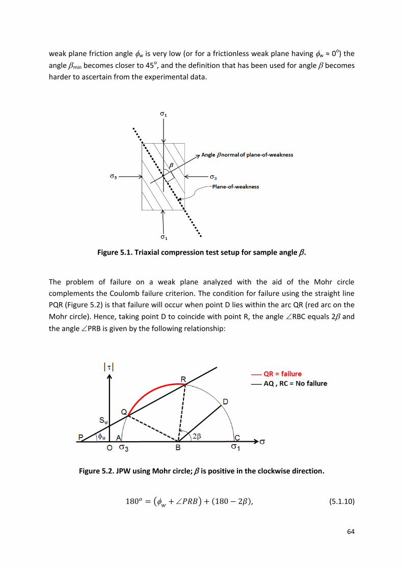
64
weak plane friction angle w is very low (or for a frictionless weak plane having w ≈ 0o) the
angle min becomes closer to 45o, and the definition that has been used for angle becomes
harder to ascertain from the experimental data.
Figure 5.1. Triaxial compression test setup for sample angle .
The problem of failure on a weak plane analyzed with the aid of the Mohr circle
complements the Coulomb failure criterion. The condition for failure using the straight line
PQR (Figure 5.2) is that failure will occur when point D lies within the arc QR (red arc on the
Mohr circle). Hence, taking point D to coincide with point R, the angle RBC equals 2 and
the angle PRB is given by the following relationship:
Figure 5.2. JPW using Mohr circle; is positive in the clockwise direction.
(
) ( ), (5.1.10)

65
. (5.1.11)
Applying the law of sine for triangles, PRB in Figure 5.2 relates to BR and PB as follows:
| | ( ) | | (
), (5.1.12)
where the terms BR and PB refer to the Mohr circle in Figure 5.2 as
| | , (5.1.13)
| | | | | |
. (5.1.14)
Rearranging Eqn. 5.1.12, the JPW criterion takes the form
| | ( ) | | (
). (5.1.15)
Inserting Eqn. 5.1.13 and 5.1.14 into Eqn. 5.1.15 yields
( ) (
)
, (5.1.16)
(
) (
). (5.1.17)
Equation 5.1.17 is the JPW criterion in Eqn. 5.1.9, but with the opposite reference angle .
Equation 5.1.9 assumes clockwise direction for angle on the Mohr-Circle (angle ABQ
increasing clockwise in Figure 5.2), whereas in Eqn. 5.1.17, angle is measured in the
counterclockwise direction (angle CBR increasing counterclockwise in Figure 5.2). Using
the same graphical approach, Eqn. 5.1.17 can be reproduced when D coincides with Q in
Figure 5.2.
To show that Q and R are the limits of the weak plane criterion, the angles CBR = 21 and
CBQ = 22 can be defined as shown in Figure 5.3. To find the relationship between 1 and
2, first find the angles BRQ and BQR as follows:
. (5.1.18)
To determine the angle BQR, subtract angle BRQ, and compute the difference of angles
22 - 21 from 180o, and input to Eqn. 5.1.18:
( ), (5.1.19)
( ) ( )
. (5.1.20)
Using the sine rule for triangles, and based on the angles BRQ and BQR in Eqn. 5.1.18
and 5.1.20, the relationship between angles 1 and 2 is found to be
| | ( ) | | ( ), (5.1.21)

66
Figure 5.3. JPW using Mohr circle; 21 and 22 are positive in the clockwise direction.
since | | | | the angles BQR and BRQ are also equal. By equating Eqn. 5.1.18 and
Eqn. 5.1.20, it follows that
, (5.1.22)
, (5.1.23)
, (5.1.24)
To determine the angle 1 as a function of { }, the angle 1 can be substituted
into Eqn. 5.1.16, after which rearrangement yields
( ) (
)
, (5.1.25)
{[(
) ] }. (5.1.26)
To determine the angle 2 as a function of { }, insert the angle 21 from Eqn.
5.1.23 into Eqn. 5.1.26 to derive the following:
{[(
) ] }. (5.1.27)
Equations 5.1.26 and 5.1.27 (Jaeger et al., 2007, p. 75, Eqn. 3.34 & 3.35) shows the range of
the angle for which sliding will occur on the weak plane within the limit angles
. The corresponding angles 21 and 22 on the Mohr circle in Figure 5.3 show these limit
angles for failure along the weak plane. The intercept point Q and R in Figure 5.3 represents
these respective orientation angles 21 and 22 of the failure envelope in Figure 5.3.
The JPW failure envelope in Figure 5.3 has a minimum within the limits
at
angle min (Figure 5.4). This point defines the inflexion point of the failure envelope defined
by the JPW criterion. By differentiating Eqn. 5.1.17, the minimum value of 1 needed for
failure is found to occur at the angle min that is related to w (Jaeger et al., 2007, p. 74) as
follows:

67
. (5.1.28)
The method of differentiating the Coulomb criterion to find the angle of minimum 1 or m
is the same for the weak plane or intact rock fracture; an example is shown in Appendix C.
An easier method to determine the angle of minimum shear strength occurring at min on
the failure envelope involves using the Mohr circle. From Figure 5.4, the failure envelope
within the limits 1 and 2 is a semicircle, and its midpoint coincides at the lowest strength
of the failure envelope at angle min. The angle 1 and 2 can each be determined as a
function of w (Eqn. 5.1.24 to Eqn. 5.1.27), and the average (midpoint) of the angle 1 and 2
is min, which is
( ) ( ). (5.1.29)
Figure 5.4. JPW model failure envelope.
It is interesting to note that the form of Eqn. 5.1.29 for failure along the weak plane is
similar to the angle o, wherein intact rock fracture occurs as per the Coulomb criterion
(Jaeger et al., 2007, p. 104, Eqn. 4.44 and Eqn. 4.46; Parry, 2000):
( ). (5.1.30)
Equation 5.1.30 has an interesting resemblance to Eqn. 5.1.29, and derives from Eqn. 5.1.28.
To explore the significance of this relationship, consider that the two angles 1 and 2 in
Eqn. 5.1.29 converge (i.e., 1 = 2 = min), in which case Eqn. 5.1.29 reduces to Eqn. 5.1.30 for
isotropic rock. In other words, when 1, 2 andmin coincide, line PQR in Figure 5.3 does not
cut through the Mohr circle. Instead, it touches the Mohr circle, resulting in an isotropic
failure condition (Eqn. 5.1.30). This means that, as the difference between the angles 1 and
2 becomes smaller, strength anisotropy is reduced. By equating Eqn. 5.1.26 and Eqn. 5.1.27
(i.e., 1 = 2), the resulting term is the isotropic failure criterion (Eqn. 5.1.4) with Sw and w
terms. Consequently, when Sw = So and w = o, strength anisotropy vanishes. These

68
relationships between the intact rock and weak plane criteria are possible because both
equations were derived from the Coulomb criterion.
Another demonstration that both Eqn. 5.1.17 and Eqn. 5.1.9 are the same, but with
different reference direction, can be carried out by using the Mohr circle diagram on Figure
5.2. The angle in Eqn. 5.1.17 is defined as increasing “counterclockwise” (21 = angle
CBR). Using the same definition, the complementary angle to 21 is therefore (21 =
angle ABR). Replacing angle 21 with 21 in Eqn. 5.1.17, the denominator becomes
[ (( ) )] = [ ( (
))]. (5.1.31)
Using the trigonometric relationship, ( ) , and inserting
Eqn. 5.1.31 into the denominator of Eqn. 5.1.17, it becomes obvious that Eqn. 5.1.17 and
5.1.9 are the same, but with different reference directions for the angle .
To determine the limits of angle for the JPW equation, manipulation of the equation for
the stress difference (1-3) required to cause failure is necessary. The maximum shear
stress, m, for a plane of weakness gives the stress difference relationship as a function of
and m. Jaeger et al. (2007, p. 74, Eqn. 3.25) expressed Eqn. 5.1.7 with the angle 1 (CBR in
Figure 5.2) as
( )
. (5.1.32)
Multiplying Eqn. 5.1.32 with
results in
(
)
. (5.1.33)
Multiplying Eqn. 5.1.33 with
results in
(
) (
)
. (5.1.34)
Using the trigonometric relationship ( )
into
Eqn. 5.1.34 gives
( ) (
)
, (5.1.35)
(
)
( ). (5.1.36)
Equation 5.1.36 (Jaeger et al., 2007, p. 74, Eqn. 3.26) expressed in terms of principal stresses
are
( ) (
( ))
( ), (5.1.37)
( ) {
(
)} {( )
(
)},

69
( ) {( ) (
)} {
(
)},
[ (
)] [
(
)]
( )
[ ( )
] [ (
)
]
. (5.1.38)
Equation 5.1.38 (Jaeger et al., 2007, p. 74, Eqn. 3.27) further simplified gives
{( )[ ( )]
} (
) , (5.1.39)
{( )[
]
} (
) ,
( )[ ]
. (5.1.40)
Using the trigonometry identity { } in Eqn. 5.1.40 yields
( )[ ( ) ]
,
( )[
]
. (5.1.41)
To simplify the above equation, replace Eqn. 5.1.41 with
( )[
]
,
( )[
]
,
( )[ (
)]
,
( ) (
) { (
)}. (5.1.42)
Equation 5.1.42 (Jaeger et al., 2007, p. 74, Eqn. 3.28) shows the stress difference that is
needed to cause failure as a function of , for a fixed value of 3. From Eqn. 5.1.42, it can be
seen that the stress difference 1 3 approaches infinity or becomes negative when β ≤ w
and β = /2. This means that the failure along the weak plane will only occur for angles
within the limits w < β < /2, as shown in Figure 5.5 (Jaeger et al., 2007, p. 104).
By inserting the principal stress ratio into Eqn. 5.1.38, the stress difference
term as a function of the stress ratio (Jaeger et al., 2007, p. 75, Eqn. 3.2.9) can be
expressed as

70
[ ( )
] [ (
)
]
,
[ ( )
(
)
]
,
[ ( )( ) ( )
]
,
[ (
)( ) ( )
]. (5.1.43)
Figure 5.5. JPW model failure envelope for limit angle w < β < /2.
Equation 5.1.43 (Jaeger et al., 2007, p. 74, Eqn. 3.29) allows a further generalization of the
plane of weakness criterion to determine stress ratio 1/3 in terms of β and w, which is
useful to determine practical values of 1/3 that are required for failure to occur.
5.2 Jaeger plane of weakness model applied to data
Triaxial experiments conducted on the Bossier and Vaca Muerta shales provide the principal
stresses 1, 3 and angle at failure. Using these strength data, anisotropic rock strength
properties o, So, w and Sw are derived for JPW model and compared against experimental
data and evaluated.
In the past, the most common method of determining the strength properties has been by
using the Mohr circle construction (e.g., Donath, 1961; Hoek, 1964; Chenevert and Gatlin,
1964; McLamore and Gray, 1967; Handin, 1969 and Donath et al., 1972). The principal
stresses at failure, 1 and 3, for different angles using graphical construction of the Mohr
circles were used to determine the slope and intercept defining the strength properties o,

71
So, w, and Sw. Jaeger (1960, 1964, 1966 and 1971) however, was more inclined to use m
versus m plots. This is the same as using Mohr circles, but is easily implemented into simple
programs to determine the strength properties o, So, w, and Sw.
Both the methods of Mohr circles and using m versus m can be implemented into a
computer program to determine the strength properties of the rock and weak plane. A
simple approach outlined here shows an example of using linear regression of best-fit
equations using m versus m, which is easily evaluated using commonly available programs
such as Excel.
The linear equation plots of maximum shear strength, m, versus mean normal stress, m, in
Figure 5.6 show the best-fit equations for angles from 0o to 90o. Figure 5.6a shows the plot
for Bossier shale, and Figure 5.6b is for Vaca Muerta shale. The m versus m plot at different
angles gives the slope and intercept that represents the linear Coulomb criterion.
For intact rock fracture, the Coulomb criterion is
. (5.2.1)
From Eqn. 5.2.1, the slope of this equation is
, (5.2.2)
( ). (5.2.3)
The friction angle of the rock, o, determined in Eqn. 5.2.3 is then used to evaluate the
cohesion So, from the intercept Co of the linear Eqn. 5.2.1:
, (5.2.4)
( )
. (5.2.5)
For failure along a weak plane, the JPW criterion is:
(
) [ ( )]. (5.2.6)
To determine the strength properties of a weak plane, the angles where failure occurs only
along the weak plane are used. This normally occurs around angles of 45o to 75o, but may
vary depending on rock type. Distinguishing the samples with weak plane failure is
important, because angles lying outside this range may not be representative of the weak
plane strength properties, w and Sw. The slope mw for m versus m plot at angles 45o, 60o
and 75o (Figure 5.6a) in Eqn. 5.2.6 is
(
), (5.2.7)
( )=
, (5.2.8)

72
Figure 5.6a. Bossier shale m vs. m plots at varying angles to determine best-fit
equation.
Figure 5.6b. Vaca Muerta shale m vs. m plots at varying angles to determine best-fit
equation.
Sw = 1694.8 psi
y = 0.5981x + 2471.2R² = 0.9676(β=90)
y = 0.4811x + 2924.8R² = 1(β=75)
y = 0.504x + 749.37R² = 0.9952(β=60)
y = 0.4572x + 1710.2R² = 0.9949(β=45)
y = 0.4677x + 2326.7R² = 0.9763(β=30)
y = 0.4835x + 4480.8R² = 0.9546(β=0)
0
5,000
10,000
15,000
20,000
25,000
0 5,000 10,000 15,000 20,000 25,000 30,000 35,000
τ m
σm
β=90
β=75
β=60
β=45
β=30
β=0
y = 0.436x + 4733.6R² = 0.9871 (β=90, 80)
y = 0.4438x + 3109.6R² = 0.9788 (β=40,50, 60, 75)
y = 0.476x + 3844.8R² = 0.9903(β=0, 10,15,20)
0
5,000
10,000
15,000
20,000
25,000
30,000
0 10,000 20,000 30,000 40,000 50,000 60,000
m
σm
Vaca Muerta - Calcareous mudstone (Unit: Psi)τm vs σm
β=90
β=50,60,75
β=0, 10, 15, 20,30,40
Linear (β=90)
Linear (β=50,60,75)
Linear (β=0, 10, 15, 20,30,40)

73
( )=
, (5.2.9)
after which dividing Eqn. 5.2.9 by
and rearranging, gives the weak plane friction angle
w as
{( ) ( )}. (5.2.10)
To determine the weak plane cohesion, Sw, the intercept Cw from the linear Eqn. 5.2.6 is
(
), (5.2.11)
( )
. (5.2.12)
The approach described from Eqn. 5.2.1 to 5.2.12 gives the same results using the Mohr
circle construction. This was verified separately in this study.
Despite the ease of using linear equations, this approach does not give strength parameters
representative of the complete data set. The reason is that it is not clear from the strength
data at which angles the intact rock fracture or failure along weak planes occurs. The plots
on Figure 5.6a,b show that the slopes and intercepts for intact rock fracture and failure
along weak planes do not vary significantly. This causes difficulty in distinguishing
representative failure modes and assigning the correct criterion at corresponding angles
This approach results in poor estimation of the strength parameters o, So, w, and Sw at
angles where the failure mode is transitioning (Chapter 4 for definition of the transition
zone) from intact rock fracture to sliding along the weak plane.
An alternative approach to determine the strength parameters representative of the
complete data set is proposed in this study. The same basic input data are used, namely the
strength data at failure, 1, the confining stress 3, and the corresponding angle . Using
this input data, a Matlab code was written to determine the JPW strength parameters that
are most representative of the complete data set (Appendix B1 and B2).
There are two parts to this Matlab code. The first part of the code (Appendix B1) contains
the three input parameters (1, 3 and angle ) and defines the objective function. The
objective function in this case is the failure criterion used for intact rock fracture (Eqn. 5.2.1)
and failure along weak planes (Eqn. 5.2.6). These two equations are applied with input data
obtained experimentally (1, 3 and angle ), for different values of strength parameters
( o,So, w,Sw) described in the main loop code.
The main loop is the second part of the code (Appendix B2) which defines the range of
strength parameters ( o,So, w,Sw) iteratively. For the selected range of strength parameters,
an output strength 1predict is calculated. The difference between the input strength 1 and
output strength 1predict determines the deviation of the model. This deviation between

74
strength data 1 and predicted strength 1predict using the root mean squared error (RMSE),
indicates the deviation of the model prediction from actual data. The RMSE is calculated as
√
∑ ( ) ( )
. (5.2.13)
The combination of strength parameters ( o,So, w,Sw) with the lowest RMSE is then saved as
the best-fit strength parameters for the selected interval.
The above-described process is repeated iteratively until the optimal strength parameters of
the rock are determined. For instance, the first range assigned for cohesion (So and Sw) is
from 0 psi to 95,000 psi, while for the friction angle ( o and w) the range is 0o to 95o. This
broad range used as a first guess covers the strength properties that are applicable for most
rock types, according to data available from the literature. In order to find the best fitting
parameters to within, say, the nearest 1 psi and the nearest 0.1 degree, one could traverse
the entire parameter space in increments of 1 psi and 0.1 degrees. However, this is not
computationally feasible. Instead, the search is first done using increments of 1,000 psi, and
5 degrees. Once the best-fitting parameters are found on this grid, the grid is refined, and
the search is repeated, but over a narrower range that is centered on the parameter values
found in the previous iteration. In this way, the optimum parameters can be found after
about three to five such iterations. The code used to determine the best-fit strength
parameters for Bossier shale are given in Appendices B1 and B2.
A brief explanation on the operations of the Matlab code is described here. Appendix B1 is
defined as the JPW model objective function, and in this code the experimental data (i.e.,
1, 3 and ) are input, followed by the equations that define the Coulomb criterion for
intact rock fracture and JPW criterion for weak plane failure. At the end of the B1 code are
the plot functions that are useful for plotting the fit data for the JPW model with least
RMSE.
The code in Appendix B2 is used to input the Coulomb parameters (i.e., So, w, Sw, w) that
are tested iteratively using the data set and equations defined in B1. The output Coulomb
parameters with least RMSE are then fit to the complete dataset, and the process is
repeated until the Coulomb parameters with lowest RMSE is determined for the dataset
input into B1. The basic concept described here is also applicable for the Pariseau model
Matlab codes in B3 and B4, wherein the Coulomb parameters are replaced by the Pariseau
parameters.

75
5.2.1 Bossier shale data analyzed using the JPW model
The discussion in Section 5.2 shows how the JPW strength properties are determined. The
failure criterion relationship of strength, 1 or m, varies as a function of 3 and angle ,
whereby the JPW model strength is a maximum at angle = 0o or 90o and a minimum at =
45 + w/2. In this section, the Bossier shale experimental data are analyzed using the JPW
model. The JPW model analysis uses the Matlab code described in the earlier section
(Appendices B1 and B2).
The JPW model failure envelope in Figure 5.7 shows the Bossier shale JPW model-predicted
strength, 1 (on the y-axis), versus the angle (on the x-axis) at different confining stresses
3, shown as solid lines. On the same plot, solid squares indicate the experimental data from
triaxial compression tests that were used to determine the JPW model strength properties.
The vertical red dotted line in Figure 5.7 is the theoretical minimum at the angle = 45 +
w/2, while the strength properties for the Bossier shale are summarized in a box at the
bottom right corner of Figure 5.7.
Figure 5.7. Bossier shale fit with the JPW model using RMSE.
For the Bossier shale samples (Figure 5.7), thirty-six triaxial compression tests were
conducted for samples with bedding angles ranging from = 0o to 90o, at confining stresses
of 0 psi, 1,000 psi, 3,000 psi, 6,000 psi and 10,000 psi. All of the samples showed increased
strengths at higher confining stresses. The general strength response shows maximum
strengths at angles of = 0o and 90o, with a minimum strength occurring at approximately
0 10 20 30 40 50 60 70 80 900
0.5
1
1.5
2
2.5
3
3.5
4
4.5
5x 10
4
βmin, 57.0
0
5,000
10,000
15,000
20,000
25,000
30,000
35,000
40,000
45,000
50,000
0 10 20 30 40 50 60 70 80 90
σ1
(p
si)
angle
Jaeger Plane of Weakness - Bossier shale
σ3= 0
σ3= 1,000
σ3= 3,000
σ3= 6,000
σ3= 10,000
JPW σ3 = 0
JPW σ3 = 1,000
JPW σ3 = 3,000
JPW σ3 = 6,000
JPW σ3 = 10,000
βmin
o = 29.0 degSo = 3750 psi
w = 24.0 degSw = 2050 psi

76
60o. The unconfined compressive strength (UCS) showed a significant difference between 0o
and 90o, with the strength at 0o being more than three times the strength at 90o. The reason
for this result is that at = 0o, the sample failed by shear in the sample matrix, whereas at
= 90o, failure occurred due to tensile splitting (Figure 4.1b). At these angles with higher
confining stresses of 1,000–10,000 psi, failure occurs predominantly by shear. Therefore,
the strength response under unconfined conditions does not have the same profile as for
samples under non-zero confining stress. For the samples tested at confining stresses of
1,000–10,000 psi, the strengths at 0o and 90o are not equal, with slightly higher strengths
observed at = 90o. Overall, the compressive strength response shows a smooth change in
strength as a function of with an RMSE value of 4,171 psi.
However, Figure 5.7 for Bossier shale shows a transition zone between about 10o and 35o,
wherein the JPW model overestimates the strength, resulting in an increased RMSE value
for the model prediction. In this regime, the strength of the shale is lower than the strength
of either the shale matrix, or the plane of weakness, which is not consistent with the JPW
conceptual model. In this transition zone, mixed-failure mode occurs due to competition of
shale matrix and weak planes causing an uneven distribution of high stresses, resulting in
shale failure at lower strength than the JPW model prediction. Also, the mixed-failure mode
causes the transition from shear fracture to sliding on a weak plane to occur over a range of
angles <1 and >2, rather than exclusively between 1 and 2, as predicted by the JPW
model; see Figure 5.5 for the definitions of 1 and 2.
In summary, the JPW model for the Bossier shale is mostly consistent with theoretical
predictions. However, the JPW model does not correctly predict the strength in the
transition zone. The JPW model also does not correctly represent the strength predictions at
unconfined conditions. The difference in accuracy between the data and the model is mainly
caused by the poor model predictions in the transition zone 10o < < 35o, where the JPW
model overestimates the strength.
5.2.2 Vaca Muerta shale data analyzed using the JPW model
Figure 5.8 shows the triaxial compression data for the Vaca Muerta shale, along with the
strength properties determined using the JPW criterion. This plot shows the experimental
data from the triaxial compressive strength 1 at varying angles , plotted as solid squares,
while the JPW model is represented by the solid lines.
Twenty-one samples were tested at confining stresses of 0 psi, 1,000 psi, 2,500 psi, 5,000
psi, and 20,000 psi. Most of the samples were tested at a confining stress of 2,500 psi to
obtain the full-failure curve as a function of , while the three compressive strength tests
conducted at 20,000 psi confining pressure were conducted to investigate the strength at
very high confining stresses. Compared to the Bossier shale, the Vaca Muerta shale fit using

77
JPW model has better fit with RMSE of 1,851 psi. All of the Vaca Muerta shale samples show
increased strengths at higher confining stresses, with maximum strengths at = 0o and 90o,
while the lowest strength occurred at = 60o. The strength response for Vaca Muerta shale
samples at angles 10o < < 40o does not show a significant difference in strength from the
value at = 0o, which is different from the Bossier shale, which showed a sharper variation
in strength with angle . One sample showed an unexpectedly higher strength at a confining
stress of 5,000 psi and an angle of = 80o; this was likely due to sample heterogeneity.
Overall, the compressive strength response for the Vaca Muerta shale shows a sharper
change in strength with angle , as compared to the Bossier shale. The Vaca Muerta shale
exhibited a nearly uniform strength in the range of angles 0o< < 40o, and did not show any
transition zone; its behavior was therefore qualitatively consistent with the assumptions of
the JPW model.
Figure 5.8. Vaca Muerta shale fit with the JPW model using RMSE.
5.3 JPW Strength anisotropic ratio (SAR)
Strength anisotropic ratio (SAR) is defined as the ratio of the average strength at the two
angles of = 0o and 90o, divided by the (minimum) strength at angle min = 45 + w/2. In this
section, the SAR value using the JPW criterion (SAR-JPW) is compared against experimental
data to predict strength anisotropy with confining stress 3 using strength parameters
derived from the Coulomb criterion (i.e., o,So, w,Sw).
0 10 20 30 40 50 60 70 80 900
1
2
3
4
5
6
7
8x 10
4
βmin, 58.0
0
10,000
20,000
30,000
40,000
50,000
60,000
70,000
80,000
0 10 20 30 40 50 60 70 80 90
σ1
(p
si)
angle
Jaeger Plane of Weakness - Vaca Muerta
σ3= 0
σ3= 1,000
σ3= 2,500
σ3= 5,000
σ3= 20,000
JPW σ3 = 0
JPW σ3 = 1,000
JPW σ3 = 2,500
JPW σ3 = 5,000
JPW σ3 = 20,000
βmin
o = 27.0 degSo = 4850.0 psi
w = 26.0 degSw = 2650.0 psi

78
The ISRM (1981) defines SAR as the strength perpendicular to the planes of anisotropy
(maximum strength) to the strength in the weakest direction (Saroglou and Tsiambaos,
2007b). Meanwhile, Ramamurthy (1993) only considered the unconfined (UCS) condition,
and defined SAR as the maximum UCS strength over the minimum UCS strength. Neither of
these approaches clearly defines SAR as a function of confining stress, 3.
Combining the ISRM definition with the JPW model, an equation to express SAR at varying
stress levels is proposed in this study. The failure criteria for intact rock fracture, and failure
along the weak plane, are
, (5.3.1)
(
) [ (
)]. (5.3.2)
Figure 5.9 shows the intact rock fracture strength at a (= 0o) and b (= 90o) divided by the
minimum strength for failure along the weak plane at c (min = 45 + w/2). Inserting the
angle min into Eqn. 5.3.2 for the minimum strength, and using the Coulomb Eqn. 5.3.1 for
intact rock fracture, the SAR-JPW is
[
] [
]. (5.3.3)
The denominator of Equation 5.3.3, which is the failure criterion for failure along the weak
plane, resembles the Coulomb criterion for intact rock fracture, because when min = 45 +
w/2 is inserted into Eqn. 5.3.2, ( ) , and the angle disappears from the
equation.
Figure 5.9. SAR defined using the JPW model.
The SAR-JPW in Eqn. 5.3.3 expressed in terms of m and m does not clearly show how
strength, 1, varies with confining stress, 3. By inserting ( ) and
( ) into Eqn. 5.3.1 and 5.3.2, the SAR-JPW of strength 1 can be expressed as a
function of confining stress 3 and strength parameters o, So, w, and Sw as

79
[ ( )
( ) ] (
). (5.3.4)
The Bossier shale SAR data compared to the SAR-JPW value in Figure 5.10 shows that SAR
reduces with increasing confining stress, 3. The SAR-JPW value (solid red line) in Figure 5.10
shows a reducing SAR, but at a lesser rate compared to the actual SAR computed directly
from the data (solid blue line with data points).
Figure 5.10. SAR-JPW plot for Bossier shale.
Figure 5.11. SAR-JPW plot for Vaca Muerta shale.
0.0
0.4
0.8
1.2
1.6
2.0
2.4
2.8
3.2
3.6
0 2,000 4,000 6,000 8,000 10,000
SAR
3 in psi
Bossier shale
SAR data
SAR JPW
Isotropy line
SAR
0.0
0.4
0.8
1.2
1.6
2.0
2.4
2.8
3.2
3.6
0 2,000 4,000 6,000 8,000 10,000 12,000 14,000 16,000 18,000 20,000
SAR
3 in psi
Vaca Muerta
SAR data
SAR JPW
Isotropy line

80
This difference between the SAR-JPW and the SAR computed directly from the experimental
data is consistent with the strength predictions observed for the Bossier shale (Figure 5.7),
whereby the model shows poor fit at unconfined (UCS) stress condition, gradually improving
to a better fit at higher confining stresses. Since the SAR-JPW model is derived from the
Coulomb criterion, the poor fit for the Bossier shale, similar to the JPW model, is expected.
This also means that the SAR-JPW value is less reliable at unconfined conditions, but shows
closer agreement to experimental data at higher confining stresses. This may be due to the
fact that the Bossier shale has high strength anisotropy and is poorly represented by the
JPW criterion, with significant error around the transition zone. The Bossier shale SAR data
and SAR-JPW are also very different because SAR-JPW is derived using averaged Coulomb
parameters over the different stress levels. These averaged parameters are unable to
capture the actual change in high SAR data with varying stress. More experiments for
different types of high SAR shales may be necessary to improve the understanding of this
behavior.
For the Vaca Muerta shale, the SAR-JPW values, compared to data in Figure 5.11, show
better agreement between model and experimental data, with lower SAR at higher
confining stresses. The SAR-JPW (solid red line) shows a good fit to the experimental data
(solid blue line with data points), displaying the reducing trend of SAR at increased confining
stress. This good agreement with SAR-JPW is also observed for the strength predictions of
the Vaca Muerta shale (Figure 5.8), which shows a good fit with the JPW strength model. In
summary, for the Vaca Muerta shale, the SAR-JPW successfully predicts strength anisotropy
from unconfined stress condition to higher confining stress up to 3 = 20,000 psi. This may
be due to the fact that the Vaca Muerta shale has low strength anisotropy, and is
represented reasonably well by the JPW criterion.
5.4 JPW model applied to triaxial extension
For many years, various researchers studied the roles of 2 for failure of isotropic rocks.
Mogi (1967) demonstrated the effect of 2 for Dunham dolomite and Westerly Granite,
observing that the fracture angle for triaxial compression and extension are notably
different. The difference in fracture angle and higher strength for extension than
compression suggests that the role of 2 cannot be ignored. In the same study, Mogi (1967)
also studied the Solenhofen Limestone, observing that compression and extension failure
strength are the same, suggesting that the role of 2 is not significant. However, the
Solenhofen limestone triaxial extension results reported by Mogi had a lower fracture angle
than in compression (Mogi, 2007). This inconsistency is not fully understood when only
principal stresses are evaluated, without having a closer look at the fracture angle .
Pariseau (2012a) explained the importance of a symmetry requirement for failure criteria
and highlighted that since most criteria are plotted as 1 = f(3), this symmetry requirement

81
is often overlooked. The Coulomb criterion satisfies the symmetry requirement and does
not have any deficiencies when the proper reference for failure angle is considered.
For the triaxial extension condition, it is obvious from the Mohr circle in Figure 5.12 that the
difference between triaxial compression and extension is a shift by . This shift by on the
Mohr circle is represented by = /2 on a sample and the JPW failure criterion. Applying
this shift of angle into the JPW failure criterion described in Eqn. 5.1.17 for triaxial
compression, for triaxial extension condition the failure criterion shifted by + /2 is
( ) ( ) . (5.4.1)
Using the trigonometric relationship, ( ) in Eqn. 5.4.1,
the JPW criterion for triaxial extension is
( ) ( ). (5.4.2)
Equation 5.4.2 for triaxial extension has the same magnitude as Eqn. 5.1.17 for triaxial
compression, but in opposite directions. This relationship for compression and extension is
shown graphically on the Mohr circles in Figure 5.12. Theoretically, if the role of 2 in
insignificant, the compression failure envelope on the Mohr circle forms a mirror image
relationship with the extension failure envelope, along the x-axis.
Figure 5.12. Mohr circle for triaxial compression and extension.
To determine the role of 2 for anisotropic rocks with failure along the weak plane, triaxial
compressions experiments were compared to triaxial extension for the Bossier shale and
Vaca Muerta shale. The Bossier shale triaxial compression tests at angles = 30o, 45o and

82
60o at different confining stresses 3 were compared to five triaxial extension samples. The
triaxial compression experiments were conducted at the following confining stresses 3 of 0
psi (UCS), 1,000 psi, 3,000 psi, 6,000 psi, and 10,000 psi. Figures 5.13a, b and c show the
Mohr circle plots for Bossier shale triaxial compression strengths compared against triaxial
extension strengths at the corresponding angles .
Figure 5.13a shows the triaxial extension strengths for 1 =2 = 25,000 psi and 3 = 7,085
psi. Comparing extension data to the Mohr circle for triaxial compression at 3 = 6,000 psi, it
is obvious that the Mohr circle diameters for compression and extension are approximately
the same size. Although only one extension test was made at the angle = 30o, the angle 2
can be estimated using Eqn. 5.1.24, shown as the failure envelope for the extension
strength in Figure 5.13a. For the Bossier shale triaxial compression samples at angle = 30o,
significant discrepancy was also observed from the JPW model, mainly due to the transition
zone effect. However, this transition zone effect did not show any difference in strength,
when compared to extension strength.
Two triaxial extension experiments were made for Bossier shale samples that fail along the
weak plane at angle = 45o, as shown in Figure 5.13b. Comparison between the triaxial
compression and extension at = 45o shows that the Mohr circle diameters in compression
and extension are similar.
Lastly, Figure 5.13c shows another two triaxial extension tests at angle = 60o, compared to
triaxial compression strengths at the same angle. The extensional strength at the lower
stress level shows the same Mohr circle diameter as does the compressive strength at the
same stress level. For the extension test at higher stress levels, interpolating between the
stress levels confirms that the diameter of the Mohr circle in compression and extension
have nearly the same size. The slope and intercept of the samples strength in compression
and extension also do not differ significantly.
For failure along the weak plane at angle = 30o, only one sample was tested under triaxial
extension conditions. Comparison between compression and extension is also possible using
a 1 versus 3 plot (described in Chapter 3). However, by comparing compression and
extension using Mohr circles, the differences in strength are more easily distinguishable. In
summary, using the Mohr circle to compare one triaxial extension sample at = 30o, and
two triaxial extension samples each at = 45o and = 60o, there is a clear trend indicating
that the Bossier shale samples do not have significantly higher strengths in extension tests
than in the compression tests. This means that for the Bossier shales, for samples that fail
along the weak plane, the role of 2 is not significant.

83
Figure 5.13a. Bossier shale triaxial compression and extension at angle = 30o.
Figure 5.13b. Bossier shale triaxial compression and extension at angle = 45o.
y = 0.332x + 1614.2R² = 0.9879
y = -0.3443x - 691.39
R² = 1
-16,000
-12,000
-8,000
-4,000
0
4,000
8,000
12,000
16,000
-5,000 0 5,000 10,000 15,000 20,000 25,000 30,000 35,000 40,000 (psi)
(psi)
= 300β=30 ; σ1 = 6,575 ; σ3 = UCS
β=30 ; σ1 = 13,320 ; σ3 = 1,000
β=30 ; σ1 = 19,365 ; σ3 = 3,000
β=30 ; σ1 = 24,492 ; σ3 = 6,000
β=30 ; σ1 = 36,200 ; σ3 = 10,000
β=30 ; σ1 = 25,000 ; σ3 = 7,085
30 deg compression
30 deg extension
Only one extension data was
available (@ 1=25kpsi), while second point was obtained using the relationships:-
(1+2)/2 = (45+ w/2) and assuming w is the same in compression and extension.
y = 0.462x + 1629.3
R² = 0.9948
y = -0.3911x - 2282.3
R² = 1-16,000
-12,000
-8,000
-4,000
0
4,000
8,000
12,000
16,000
-5,000 0 5,000 10,000 15,000 20,000 25,000 30,000 35,000 40,000 (psi)
(psi)
= 450
β=45 ; σ1 = 5,655 ; σ3 = UCS
β=45 ; σ1 = 8,020 ; σ3 = 1,000
β=45 ; σ1 = 15,680 ; σ3 = 3,000
β=45 ; σ1 = 22,720 ; σ3 = 6,000
β=45 ; σ1 = 32,555 ; σ3 = 10,000
β=45 ; σ1 = 8,020 ; σ3 = 229
β=45 ; σ1 = 25,000 ; σ3 = 7,661
45 deg compression
45 deg extension
Linear (45 deg compression)
Linear (45 deg extension)

84
Figure 5.13c. Bossier shale triaxial compression and extension at angle = 60o.
For the Vaca Muerta shales (Figure 5.14a and b), three triaxial extension experiments were
attempted, at angles = 0o, 90o and 60o. From the two samples tested under triaxial
extension conditions at angles = 0o and 90o, the extension sample at angle = 90o did not
fail in shear, due to end effects (Figure 4.4b), resulting in lower shear strength failure by
splitting. This sample at angle = 90o was excluded from the extension result shown in
Figure 5.14a, and is not included in the analyses described here. Only the sample at angle
= 0o, which sheared sufficiently through the intact rock, shows significantly higher strength
than did the triaxial compression sample. Figure 5.14a shows the Mohr circles for triaxial
compression at angles = 0o and 90o, compared to the triaxial extension at = 0o. The
comparison between the triaxial compression and the triaxial extension at 3 = 1,000 psi
shows that the diameter of the Mohr circle for triaxial extension is approximately 5,000 psi
larger than that for triaxial compression. This means that the sample under triaxial
extension is stronger than under triaxial compression, and hence underscores the
importance of the role of 2 for intact rock failure for the Vaca Muerta shale.
Only one sample was selected for the Vaca Muerta shale triaxial extension test for failure
along the weak plane at angle = 60o. This was mainly done to see if the result observed for
the Bossier shale, indicating an insignificant role of 2, is also observed for Vaca Muerta.
Figure 5.14b shows one triaxial extension sample with principal stresses 1 =2 = 22,619 psi
failed at 3 = 3109 psi, but there are no triaxial compression experiments for 3 close to
3,000 psi for direct comparison. However, the average of the triaxial compression Mohr
circles for 3 = 1,000 psi and 5,000 psi shows that the diameters of the Mohr circles for
triaxial compression and extension are of approximately the same size. This means that the
y = 0.5823x + 875.92
R² = 0.9914
y = -0.4838x - 2079.6
R² = 1
-16,000
-12,000
-8,000
-4,000
0
4,000
8,000
12,000
16,000
-5,000 0 5,000 10,000 15,000 20,000 25,000 30,000 35,000 40,000
(psi)
(psi)
= 600
β=60 ; σ1 = 1,810 ; σ3 = UCS
β=60 ; σ1 = 6,670 ; σ3 = 1,000
β=60 ; σ1 = 13,750 ; σ3 = 3,000
β=60 ; σ1 = 20,330 ; σ3 = 6,000
β=60 ; σ1 = 33,195 ; σ3 = 10,000
β=60 ; σ1 = 25,000 ; σ3 = 7,190
β=60 ; σ1 = 13,320 ; σ3 =2,610
60degrees compression
60 degree extension
Linear (60degrees compression)
Linear (60 degree extension)

85
Figure 5.14a. Vaca Muerta shale triaxial compression and extension at angle = 0o.
Figure 5.14b. Vaca Muerta shale triaxial compression and extension at angle = 60o.
y = 0.5762x + 4353.1
R² = 0.9565
-20,000
-16,000
-12,000
-8,000
-4,000
0
4,000
8,000
12,000
16,000
20,000
-10,000 -5,000 0 5,000 10,000 15,000 20,000 25,000 30,000 35,000 40,000
(psi)
(psi)
= 00 and 900
β=0 ; σ1 = 13,730 ; σ3 = UCS
β=90 ; σ1 = 19,075 ; σ3 = 1,000
β=0 ; σ1 = 20,120 ; σ3 = 1,000
β=90 ; σ1 = 21,845 ; σ3 = 2,500
β=90 ; σ1 = 27,675 ; σ3 = 5,000
β=0 ; σ1 = 30,745 ; σ3 = 5,000
β=90 ; σ1 = 67,000 ; σ3 = 20,000
β=0 ; σ1 = 69,965 ; σ3 = 20,000
βcomp=90 ; σ1 = 25,000 ; σ3 =1,150
beta fracture angleTXC
Linear (beta fractureangle TXC)
y = 0.496x + 2888.9
R² = 0.9962
-25,000
-20,000
-15,000
-10,000
-5,000
0
5,000
10,000
15,000
20,000
25,000
-10,000 0 10,000 20,000 30,000 40,000 50,000 60,000 70,000
(psi)
(psi)
= 600
β=60 ; σ1 = 7,874 ; σ3 = UCS
β=60 ; σ1 = 12,335 ; σ3 = 1,000
β=60 ; σ1 = 23,915 ; σ3 = 5,000
β=60 ; σ1 = 61,000 ; σ3 = 20,000
β=60 ; σ1 = 22,600 ; σ3 =3,109
JPW angle TXC
Linear (JPW angleTXC)

86
Vaca Muerta shale triaxial compression and extension strengths are not significantly
different, which implies that the role of 2 for Vaca Muerta shale that fails along the weak
plane can be ignored. This outcome for Vaca Muerta shale at = 60o also verifies the results
observed for the Bossier shales.
In summary, using Mohr circles to compare the triaxial compression and extension test data,
it can be said that the strength for intact rock failure are much higher for extension tests.
For weak plane failure, strength in compression and extension are not very different. This
means that the role of 2 cannot be ignored for the intact rock failure, whereas for the weak
plane failure, the role of 2 is not significant.
5.5 JPW model applied to data from literature
The Bossier shale evaluation with the JPW model in Section 5.2 shows poorer fits compared
to those obtained for the Vaca Muerta shale. Evaluation of the CT scan and thin section
images shows that the JPW model for Bossier shale had mixed failure modes with lower
strength at the transition zones, while the Vaca Muerta shale showed a good fit using the
JPW model. In this section, similar evaluations for various anisotropic rocks from the
literature are made using the JPW model, but without access to any CT or thin section
images.
The different rock types from the literature used for the JPW model analysis are the Angers
schist (Duveau et al., 1998), Martinsberg slate (Donath, 1964), Austin slate, Green River
Shale-1, Green River Shale-2 (McLamore and Gray, 1967), Quartz Phyllite, Carbona Phyllite,
Micaceous Phyllite (Ramamurthy et al., 1993), Penrhyn slate (Attewell and Sandford, 1974)
and Tournemire shale (Niandou, 1997). All data sets in this study are presented in units of
psi, as this will facilitate comparing strength parameters for different rock types (Appendix
D1).
Table 5.1 outlines the results of analysis for anisotropic rocks from experiments and the
literature, using the JPW model. The first three columns show the source of the data, while
the fourth column is the RMSE (defined in Eqn. 5.2.13) showing the amount of prediction
error for different rock types. The next column is the measured strength divided by the
model prediction (1actual/1predict), which provides a slightly different type of error
measurement, indicating the average deviation of the data from the model. This gives an
approximate error measurement in terms of percentage, when multiplied by 100%.

87
Table 5.1. Summary of various data analyzed using JPW model.
No Rock type Reference RMSE (psi)
1actual
/
1predict
o
(deg) So (psi)
w
(deg) Sw
(psi) SAR
1 Bossier shale
present work 4171 0.961 29.0 3750 24.0 2050 2.017
2 Vaca Muerta shale
present work 1851 1.000 27.0 4850 26.0 2650 1.866
3 Angiers Schist
Duveau et al., 1998
3074 0.949 41.2 5200 8.2 1600 6.206
4 Martinsburg Slate
Donath, 1964
5984 0.982 30.3 7100 16.8 1900 4.836
5 Austin Slate McLamore & Gray, 1967
6385 1.007 22.2 11750 13.6 6550 2.101
6 GreenRiver Shale 1
McLamore & Gray, 1967
2166 0.997 27.8 9800 30.5 6100 1.522
7 GreenRiver Shale 2
McLamore & Gray, 1967
1811 1.004 19.2 6350 18.7 4000 1.602
8 Quartz Phyllite
Ramamurthy et al., 1993
2692 0.991 32.4 3450 25.9 2250 1.746
9 Carbona Phyllite
Ramamurthy et al., 1993
2706 0.994 32.8 3200 28.7 1800 1.932
10 Micaceous Phyllite
Ramamurthy et al., 1993
5240 0.972 35.4 3500 21.4 1500 3.084
11 Penrhyn Slate
Attewell & Sandford, 1974
6018 0.988 35.1 7010 14.7 4970 2.095
12 Tournemire Shale
Niandou et al., 1997
1448 0.982 24.1 1850 20.2 1270 1.568
After the source information, RMSE, and the ratio of 1actual/1predict, the fifth to the eight
columns of Table 5.1 show the Coulomb strength parameters determined using the best-fit
method by calculating the lowest RMSE for the combination of strength parameters for a
specific anisotropic rock type. The details of this approach were described in Section 5.2,
and the complete evaluation for different rock types with strength plots are provided in
Appendix E. The intact rocks strength parameters evaluated in this study are 19.2o < 0 <
41.2o and 1,850 psi < So < 11,750 psi, while the weak plane strength parameters are 8.2o < w
< 30.5o and 1,270 psi < Sw < 6,550 psi. This broad range of anisotropic strength properties
covers a wide range of rock types commonly encountered in the oil and gas industry.
Lastly, in the far right column, the SARs for different rock types are listed. To distinguish the
different anisotropic rock types, the SAR derived from the JPW model at UCS is adopted.
Inputting the 3 = 0 (UCS) condition into Eqn. 5.3.4, the SAR used to distinguish different
rocks types becomes
(
) (
). (5.5.1)

88
Equation 5.5.1 is the SAR derived from the Coulomb criterion with four strength parameters,
distinguishing different rock types. From this point onwards, SAR denotes the strength
anisotropic ratio calculated from Coulomb strength parameters at the 3 = 0 (UCS)
condition. For most rocks, the SAR defined in Eqn. 5.5.1 may not directly correlate with the
strength parameters derived solely from unconfined experiments, because the strength
parameters used here are averaged from experimental data at different confining stress
levels.
Comparing the RMSE and 1actual/1predict of anisotropic rocks from experiments and the
literature shows that the JPW model predicts rock strength reasonably well for most
orientations, but with increased mean error at the transition zones (see Appendix E, Figure
E1 for plot of 1actual/1predict vs. angle ). The transition zone is the angle where the failure
mode changes from shear fracture to sliding failure along the weak plane. At these
transition zones, the shear fracture changes from intact rock fracture to sliding along the
weak plane. Between these two failure modes, the rock fails in mixed modes, and for some
rocks this change is not adequately captured by the Coulomb criterion. The gradual change
in strength at transition zone results in increased RMSE for the JPW model.
Most rocks from the literature shown in Table 5.1 show higher RMSE for rocks having higher
SARs (i.e., Bossier shale, Angers schist, Martinsberg slate, Austin slate, Micaceous Phyllite
and Penrhyn slate). For these rocks with high strength anisotropy, the JPW model probably
has increased RMSE at the transition zones, whereas for the rocks with low SAR (i.e., SAR <
2.0, such as the Vaca Muerta, GRS-1, GRS-2, Quartz Phyllite, Carbona Phyllite and
Tournemire shale), lower RMSE is obtained.
From the evaluation of the various rock types in this study, it is also possible to explore the
possible shapes of the JPW model, which is a function of the four Coulomb parameters So,
o, Sw and w. The difference between So and Sw, and between o and w, determines the
shape of the strength anisotropy as a function of confining stress 3. Increases in Sw and w
generally shift the weak plane circle upwards and closer to the isotropic line. An increase in
Sw will only shift the circle upward, towards the isotropic line, moving along the centerline at
= 45 + w/2. An increase in w only will shift the weak plane circle upward closer to the
isotropic line, and sideways towards = 90o. Therefore, an increase in Sw only shifts the
circle upwards, while an increase in w shifts the circle upwards and sideways. The minimum
of the weak plane circle cannot be less than 45o because min occurs at 45+ w/2, and for
most rocks w is not equal to zero. The angle 1 also cannot be less than w, which was also
shown earlier in this chapter. These are the basics of the JPW model shapes that are a
function the four Coulomb parameters.
The more difficult aspect to understand is the shape of the failure curve for the extreme
cases where there is a significant difference in So, Sw and o, w. For most anisotropic rocks,
where So > Sw and o > o, the angles 1 increases and 2 decreases with increase in

89
confining stress 3. However, for extreme situations, 1 and 2 can also decrease and
increase with increase in 3, and this was seen for the cases presented in Appendix E for the
Angers Schist and Penrhyn Slate. These two anisotropic rocks had the highest difference in
o - w (i.e., Angers Schist o - w = 33o, and Penrhyn Slate o - w = 20.4o). These two cases
are unique, showing a slight decrease in 1, and an increase in 2 at higher confining
stresses. This is a rare scenario and could have been a consequence of the data-fitting
technique; this issue needs to be further explored.
Figure 5.15 shows a plot of the RMSE using the JPW model, against SAR, for different rock
types. In this plot, the different rock types are grouped into four categories: low SAR shales,
Shales and Phyllite, Slates, and Schist. The organic-rich mudstones in this study show higher
RMSE with SAR, while the Slates and Schist generally have higher RMSE. This plot gives a
general idea of expected RMSE for different rock types, and is useful for comparison with
other anisotropic rocks.
Figure 5.15. Summary of JPW model RMSE vs. SAR.
5.6 JPW model using reduced numbers of data sets
In this study, the JPW model applied to different rock types shows that the JPW model
provides a good fit for low SAR rocks, but has a higher mean error for high SAR rocks.
However, this JPW model evaluation for different anisotropic rocks uses significant amount
of triaxial compression data at various confining stress and bedding angles . These data
provide the necessary information to understand the complete strength behavior and to
0
1,000
2,000
3,000
4,000
5,000
6,000
7,000
0 1 2 3 4 5 6 7
RM
SE (
psi
)
SAR
1 Bossier shale
2 Vaca Muerta shale
3 Angers Schist
4 Martinsburg Slate
5 Austin Slate
6 GreenRiver Shale 1
7 GreenRiver Shale 2
8 Quartz Phyllite
9 Carbona Phyllite
10 Micaceous Phyllite
11 Penrhyn Slate
12 Tournemire Shale
Slates
Low SAR shale
Shale and Phyllites
Organic rich mudstones
Schist

90
best calibrate the JPW model. In reality, such extensive experiments with so much data
collected would not always be feasible for practical applications. Therefore, it is useful to
identify the minimum possible number of data that would be necessary to implement the
JPW model, without significantly affecting the accuracy of the fits.
To carry out the reduced data analysis for the JPW model, the data sets from experiments
and the literature are analyzed under three different conditions. The RMSE for the complete
data set at different confining stresses and angles is the base case scenario used for
comparison. The same data set RMSE is then determined with the JPW model at two
confining stress levels, covering the highest and lowest confining stresses. Lastly, the
reduced data RMSE evaluation is made at two confining stress levels, at angles = 0o, 30o,
60o and 90o. The selection of the eight data points based on earlier experimental evidence
from the Bossier and Vaca Muerta shale shows that the main changes in failure modes
occurs at these angles.
The reduced data analysis best-fit parameters are used to determine the JPW model’s
Coulomb strength parameters ( o,So, w,So), and these parameters are then used to
determine the RMSE against the complete data set available for the different rock type.
Figure 5.16 shows the comparison of the JPW model RMSE using the complete data set, the
data obtained at two stress levels at varying angles , and lastly the data obtained at two
stress levels at angles = 0o, 30o, 60o and 90o.
Figure 5.16. JPW model data using reduced data sets for various rock types.
0 1,000 2,000 3,000 4,000 5,000 6,000 7,000 8,000
Tournemire Shale
Penrhyn Slate
Micaceous Phyllite
Carbona Phyllite
Quartz Phyllite
GreenRiver Shale 2
GreenRiver Shale 1
Austin Slate
Martinsburg Slate
Angers Schist
Vaca Muerta shale
Bossier shale
Mean error (psi)
JPW All data (psi)
JPW two stresslevel (psi)
JPW two stresslevel @0,30,60,90deg(psi)

91
The JPW model analysis for the three scenarios of base case and reduced data set in Figure
5.16 shows a general trend of increasing mean errors when using reduced data sets. The
base-case scenario using complete data sets represents the ideal condition and best-fit
scenario for the JPW model at varying confining stress and bedding angles . For the
reduced data set, analysis at two confining stress levels at varying angles shows only a
slight increase in mean error compared to the base case scenario that uses all the data. This
means that although only two confining stress levels were used, the data in between these
two stress levels do not significantly improve the overall model accuracy. However, for the
case of using reduced data at two confining stress levels at angles = 0o, 30o, 60o and 90o,
rock types with high SAR showed higher increase in mean errors. The Angers Schist, for
example, shows more than a two-fold RMSE increase, while the Penrhyn Slate has an
increase of about 25% in mean error, when analyzed using data at angles = 0o, 30o, 60o
and 90o. The main reason for this is that the increased RMSE at the transition zone is not
fully captured by the data at = 30o. This suggests that for anisotropic rocks with high SAR,
the JPW model analyses using reduced numbers of data can be done without significantly
increasing RMSE at two confining stress levels, but needs data at various bedding angles
such as = 0o, 15o, 30o, 45o, 60o, 75o, and 90o. For the case of low SAR rocks, no significant
increase in RMSE was observed for both the reduced data set cases.
In summary, the JPW model analysis using reduced numbers of data shows that for most
anisotropic rock types with low SAR, eight strength values obtained at two confining stress
levels (i.e., four strength data at each stress level) at bedding angles of = 0o, 30o, 60o and
90o, would be sufficient to obtain the failure envelope without causing significant increase in
RMSE. On the other hand, for the case of rocks with high strength anisotropy, fourteen
strength data obtained at two stress levels (i.e., seven strength data at each stress level) and
bedding angles at intervals of 15o (i.e., = 0o, 15o, 30o, 45o, 60o, 75o and 90o) are required
in order to predict the JPW model failure envelope without significantly increasing the
RMSE.

92
6 Pariseau’s Model
6.1 Theory and data-fitting technique
Pariseau (1968) presented a failure model for anisotropic geological media at the 10th AIME
Symposium on Rock Mechanics in a paper entitled “Plasticity Theory for Anisotropic Rocks
and Soils”. Pariseau developed his theory by modifying Hill’s theory for metal plasticity (Hill,
1948). The main new contribution of Pariseau was the modification of Hill’s theory to
account for yielding of geomaterials under hydrostatic stress. Pariseau’s continuum model is
an extension of the Drucker-Prager model that satisfies the symmetry requirements for a
transversely isotropic material. Unlike the plane of weakness model, this model predicts a
smooth, continuous variation of strength with bedding angle .
Although Pariseau’s criterion has been available for more than forty years, few researchers
have attempted to apply it to laboratory data on reservoir rocks. Duveau et al. (1998) used
the Pariseau criterion to assess the strength of the Angers Schist and concluded that this
model is comparable in accuracy to the JPW criterion. Amadei (1983) showed that the five
Pariseau parameters (F, G, U, V and M) can be determined using simplified equations from
unconfined compressive, tensile and torsional strengths, at = 0o, 45o and 90o. However,
Amadei did not use experimental data from different rock types to verify the robustness of
this approach at different confining stresses.
Although Duveau et al. (1988) validated Pariseau’s model for the Angers schist, this model
was never validated for a range of anisotropic rocks. Pariseau’s model has similarities to the
Drucker-Prager model for isotropic rocks (i.e., it uses the stress invariants J2 and I1), as
several researchers have demonstrated (Tsai and Wu, 1971; Smith and Cheatham, 1980a;
Kusabuka et al., 1999). Ong and Roegiers (1993), using Pariseau’s model, showed that high-
strength anisotropic rocks significantly influence the stability of horizontal wells. A similar
study of wellbore stability by Suarez-Rivera et al. (2009) showed that the Pariseau strength
model, combined with an anisotropic elastic rock model, provides more conservative results
than are obtained by using the JPW strength model in combination with an isotropic elastic
model to compute the stresses.
One possible reason for the limited previous use of the Pariseau criterion is that the process
required to determine the rock parameters is not straightforward. Sufficient data
representing the failure envelope are necessary to determine the rock parameters used in
this criterion, and this process involves finding solutions to a global minima problem.
Despite these problems, the Pariseau criterion offers the attractive possibility of being a
continuous failure criterion, as opposed to the “discontinuous” JPW model. The most
exciting prospect of this model is its inclusion of the role of 2. This chapter describes the
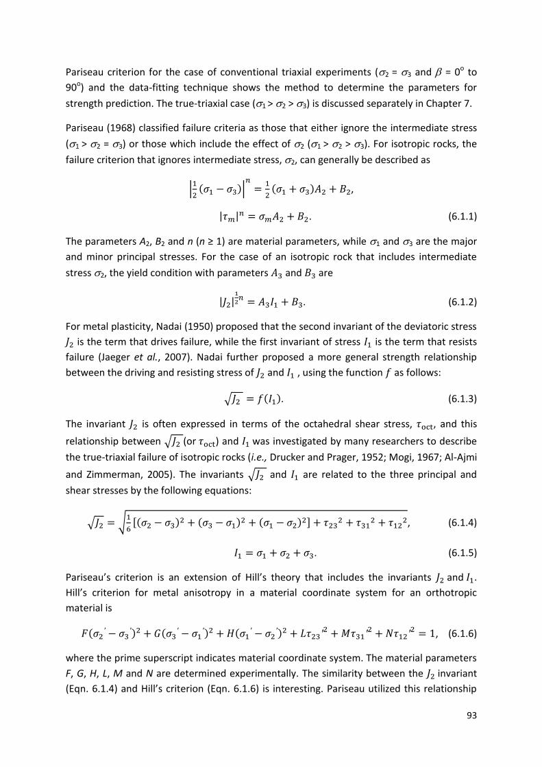
93
Pariseau criterion for the case of conventional triaxial experiments (2 = 3 and = 0o to
90o) and the data-fitting technique shows the method to determine the parameters for
strength prediction. The true-triaxial case (1 > 2 > 3) is discussed separately in Chapter 7.
Pariseau (1968) classified failure criteria as those that either ignore the intermediate stress
(1 > 2 = 3) or those which include the effect of 2 (1 > 2 > 3). For isotropic rocks, the
failure criterion that ignores intermediate stress, 2, can generally be described as
|
( )|
( ) ,
| | . (6.1.1)
The parameters A2, B2 and n (n ≥ 1) are material parameters, while 1 and 3 are the major
and minor principal stresses. For the case of an isotropic rock that includes intermediate
stress 2, the yield condition with parameters and are
| |
. (6.1.2)
For metal plasticity, Nadai (1950) proposed that the second invariant of the deviatoric stress
is the term that drives failure, while the first invariant of stress is the term that resists
failure (Jaeger et al., 2007). Nadai further proposed a more general strength relationship
between the driving and resisting stress of and , using the function as follows:
√ ( ). (6.1.3)
The invariant is often expressed in terms of the octahedral shear stress, , and this
relationship between √ (or ) and was investigated by many researchers to describe
the true-triaxial failure of isotropic rocks (i.e., Drucker and Prager, 1952; Mogi, 1967; Al-Ajmi
and Zimmerman, 2005). The invariants √ and are related to the three principal and
shear stresses by the following equations:
√ √
( ) ( ) ( )
, (6.1.4)
. (6.1.5)
Pariseau’s criterion is an extension of Hill’s theory that includes the invariants and .
Hill’s criterion for metal anisotropy in a material coordinate system for an orthotropic
material is
(
) (
) (
)
, (6.1.6)
where the prime superscript indicates material coordinate system. The material parameters
F, G, H, L, M and N are determined experimentally. The similarity between the invariant
(Eqn. 6.1.4) and Hill’s criterion (Eqn. 6.1.6) is interesting. Pariseau utilized this relationship

94
and proposed a criterion that has a similar form as the Hill’s criterion that includes the
term with parameters U, V and W to account for the yielding of geomaterials under
hydrostatic stress (Amadei, 1983):
| (
) (
) (
)
|
-(
). (6.1.7)
To determine the parameters using experimental data, Eqn. 6.1.7 is changed into the
principal coordinate system using the stress transformation equations. Figure 6.1 shows the
stress system and orientation used in the stress transformation equations. For the triaxial
stress conditions shown in Figure 6.1, the bedding angle is the normal vector of the plane
to 1, while the foliation direction is = 0o because the angle is parallel to 2 = 3 (see
also Figure 7.3 for definition of and for true-triaxial stress system).
Figure 6.1. Stress system in principal coordinate for triaxial compression.
The direction cosines that are needed to transform Eqn. 6.1.7 are (Jaeger et al., 2007, p.34):
( ) ( ),
( ) ( ),
( ) ( ). (6.1.8)
The principal and shear stresses in the material coordinate system are
;
; ; ; ; , (6.1.9)
,
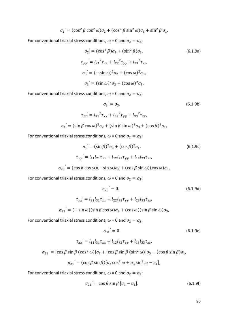
95
( ) ( ) ,
For conventional triaxial stress conditions, = 0 and ;
( ) ( ) . (6.1.9a)
,
( ) ( ) ,
( ) ( ) ,
For conventional triaxial stress conditions, = 0 and :
. (6.1.9b)
,
( ) ( ) ( ) ,
For conventional triaxial stress conditions, = 0 and :
( ) ( ) . (6.1.9c)
,
( )( ) ( )( ) ,
For conventional triaxial stress conditions, = 0 and :
. (6.1.9d)
,
( )( ) ( )( ) ,
For conventional triaxial stress conditions, = 0 and :
. (6.1.9e)
,
( ) ( ) ( ) ,
( ) ,
For conventional triaxial stress conditions, = 0 and :
. (6.1.9f)

96
For transverse isotropy along the bedding plane:
G = H, M = N, V = W, L = 2G + 4F. (6.1.10)
Inserting the parameters in Eqn. 6.1.10 into Pariseau’s equation Eqn. 6.1.7 for the case n = 1
yields
[ ( ) {( )
( )
} ( )
(
)]
[ ( )]. (6.1.11)
Solving Eqn. 6.1.11 with inputs from Eqns. 6.1.9a-f, inserting the principal stresses, and
rearranging the parameters F, G, U, V and M, results in the Pariseau equation in principal
coordinates (Pariseau, 1968, p. 281 Eqn. 26a):
( ) ( )
( ( ) ) ( )
(6.1.12)
6.2 Pariseau model applied to data
The Pariseau criterion (Eqn. 6.1.12) for conventional triaxial stress conditions (1 > 2 = 3)
was described in the previous section, wherein F, G, U, V and M are rock constitutive
parameters determined experimentally. These parameters may be determined by solving
the global minimum problem iteratively, repeated until the parameters that yield the
minimum mean error is determined. Appendices B3 and B4 show the Matlab code used for
the Pariseau model.
In this iterative approach, the initial parameters estimated covers a large interval of possible
solutions that estimates the range of possible values. Based on the estimated parameters,
the RMSE (defined in Chapter 5) is computed, and a narrower interval is then assigned. This
process is repeated until the lowest possible RMSE is obtained.
In the iterative process described above, the initial range of parameters F, G, U, V and M are
estimated. The method described by Amadei (1983) using UCS data provides a reasonably
good first estimate, but needs tensile strength data at angle =0o and 90o. To determine the
Pariseau rock parameters iteratively, it is easier if F, G, U, V and M are each expressed in
terms of strength parameters that have units of stress. This avoids the need to use very
small values of the Pariseau parameters in the calibration process. The parameters F, G, U, V
and M expressed in terms of the strength data in psi are f, g, u, v and m:
;
;
;
;
. (6.1.13)

97
An example of this iterative process is shown in Table G1 of Appendix G. The initial range for
parameters f, g, u, v and m covers a wide range of possible values, and the combination of
these parameters with lowest RMSE is determined as the new reference value for the next
iteration.
For the Matlab code used in this study, one cycle of iteration takes around five minutes, and
with further refinement (finer grid) to increase the accuracy of the model, the process could
increase to 30 minutes or beyond. However, for the accuracy that is needed for the present
purposes, a five-minute cycle was used to analyze all the data sets in this study, to an
accuracy of within 100 psi for all five strength parameters. For all the anisotropic rocks
tested in this study, when the selected grid is finer than 1,000 psi, very little change in RMSE
is observed.
The parameters f, g, u, v and m determined from the iterative process when applied into
equation 6.1.13 determine the rock parameters F, G, U, V and M. The Pariseau rock
parameters are then used in Eqn. 6.1.12 to calculate strength 1 as a function of confining
stress 3 and angle at failure. The physical interpretation of the Pariseau rock parameters
will also be explored in the following sections.
6.2.1 Bossier shale data analyzed using Pariseau’s model
In Chapter 5, the Bossier shale fit using the JPW model showed high RMSE, especially in the
transition zones. In this chapter, the same Bossier shale data set is fit using the Pariseau
model. The parameters F, G, U, V and M determined iteratively are:
Table 6.1. Summary of Pariseau Parameters for Bossier shale.
Parameters F [psi-2] G [psi-2] U [psi-1] V [psi-1] M [psi-2]
Values 2.38E-09 9.07E-09 6.67E-05 4.17E-05 1.11E-07
Inserting these parameters into Eqn. 6.1.12 provides the continuous failure envelopes
shown in Figure 6.2.
For the Bossier shale, the UCS failure envelope at different angles has a poor fit with
experimental data, and is not adequately represented using the Pariseau model. This is
because the sample at = 90o fails in tensile splitting (see the CT scans in Chapter 4),
whereas all the other samples used in this study failed in shear. The strength predicted for
the Bossier shale at angle = 90o is slightly higher than the strength predicted at angle =
0o. This was observed for samples with 3 of 1,000 psi and 10,000 psi, while at 3 of 3,000
psi and 6,000 psi the sample strength are almost the same at angles = 0o and 90o.

98
The Pariseau model for the Bossier shale provides a better fit than does the JPW model,
with RMSE of 3,248 psi, which is lower than the RMSE of the JPW model, which was 4,171
psi. Unlike the JPW model, Pariseau’s model consists of a single equation over the entire
range of angles, representing the complex transition of compressive strength from intact
rock shear fracture, mixed mode, and sliding along weak planes reasonably well. Another
attribute of the Pariseau’s model is that it is able to capture possible strength differences at
= 0o and 90o, while the JPW model assumes that strengths are equal at these angles. In
this regard, it is worth noting that the JPW model contains four adjustable parameters,
whereas Pariseau’s model contains five.
Figure 6.2. Bossier shale failure data fit by Pariseau’s model.
In summary, analysis of the Bossier shale using Pariseau’s model provides a better fit than
does the JPW model. Pariseau’s model also gives a better representation of the compressive
strengths at the transition zone. However, the same Pariseau model parameters determined
at different stress levels are not applicable for unconfined condition at angle = 90o,
because the failure mode is that of tensile splitting, resulting in lower strength.
Another observation from the analysis of the Bossier shale shows that the form of the
failure envelope can be further explored to examine what controls the minimum (for
Bossier shale min this is close to 45o) and the slight strength difference observed at = 0o
and 90o. This will be explored further in the following sections.
0
5,000
10,000
15,000
20,000
25,000
30,000
35,000
40,000
45,000
50,000
0 10 20 30 40 50 60 70 80 90
σ1
(psi
)
3=0
3=1000
3=3000
3=6000
3=10000
σ3 = 0
σ3 = 1,000
σ3 = 3,000
σ3 = 6,000
σ3 = 10,000

99
6.2.2 Vaca Muerta shale data analyzed using Pariseau’s model
Compared to the Bossier shale, the Vaca Muerta shale is less argillaceous, and has lower
strength anisotropy. In this section, the Vaca Muerta shale is fit using Pariseau’s model using
the same approach described earlier. The parameters F, G, U, V and M determined for Vaca
Muerta shale are:
Table 6.2. Summary of Pariseau Parameters for Vaca Muerta shale.
Parameters F [psi-2] G [psi-2] U [psi-1] V [psi-1] M [psi-2]
Values 6.40E-09 4.16E-09 2.99E-05 3.77E-05 4.00E-08
The Vaca Muerta shale data fit using Pariseau’s model gave an RMSE of 2,390 psi, which is
higher than the RMSE obtained using the JPW model. Applying these parameters in Eqn.
6.1.12 provides the failure envelopes shown in Figure 6.3.
The Vaca Muerta shale was tested at confining stresses from 0 psi up to 20,000 psi, and
Pariseau’s model follows the general trend of the failure envelope at all the tested stress
levels. Looking in detail, the difference in RMSE between the Pariseau and JPW model for
the Vaca Muerta shale is mainly due to the increased errors near = 40o, where the smooth
transition zone occurred for the Bossier shale. This transition zone does not occur for Vaca
Muerta, resulting in higher RMSE for Pariseau’s model.
Figure 6.3. Vaca Muerta shale failure data fit using the Pariseau’s model.
0
10,000
20,000
30,000
40,000
50,000
60,000
70,000
80,000
0 10 20 30 40 50 60 70 80 90
σ1
(psi
)
3=0
3=1000
3=2500
3=5000
3=20000
σ3=UCS
σ3 = 1000 psi
σ3 = 2,500 psi
σ3 = 5,000 psi
σ3 = 20,000 psi

100
In summary, the Vaca Muerta shale yields a higher RMSE when analyzed using Pariseau’s
model than with the JPW model. This is despite the fact that Pariseau’s model contains one
more adjustable parameter than does the JPW model. The Vaca Muerta shale has low
strength anisotropy, and does not exhibit any significant transition zone, as had been
observed for the Bossier shale. Based on this comparison, it can be concluded that
Pariseau’s model gives a poorer fit than does the JPW model, for the Vaca Muerta shale.
6.3 Pariseau Strength Anisotropy Ratio (SAR)
The strength anisotropy ratio (SAR) for the JPW model was defined in Section 5.3, where it
was discussed in light of the JPW model. Using the same approach, this section attempts to
quantify SAR using the Pariseau model; the numerical value will be denoted by SAR-
Pariseau. SAR-Pariseau is the ratio of maximum to minimum strength at a specified
confining stress level, as determined by the equation that has been fitted to the laboratory
failure data.
The SAR for Pariseau’s model is used to determine if the model is able to capture the
reducing strength anisotropic behavior of shales at higher stress levels. It is straightforward
to use Pariseau’s failure criterion in Eqn. 6.1.12 to define the SAR equation. According to
Pariseau’s model, unlike the JPW, there can be differences in the maximum strength at
angles = 0o and 90o. From Eqns. 6.3.1 and 6.3.2, the ratio of maximum strength at = 0o
and 90o to minimum strength at min can be determined. For the case of = 0o and 90o, the
strength defined in Eqn. 6.1.12 reduces to the following expressions, respectively:
( ) ( )
( ) ( ) (6.3.1)
( ) ( )
( ) ( ). (6.3.2)
Using Pariseau’s equation, the minimum strength at min can be determined by
differentiating Eqn. 6.1.12, to find that its minimum occurs at an angle given by
[(
)
], (6.3.3)
Similar to the approach used for the SAR-JPW model, using the results from Eqn. 6.3.1, Eqn.
6.3.2 and Eqn. 6.3.3, SAR-Pariseau can be expressed as
[
( ) ( )
( ) ( )]
{
( ( ) ) ( )}
(6.3.4)

101
Equation 6.3.4 cannot be further simplified, and remains a relatively complicated equation,
containing all five Pariseau parameters, {F, G, U, V, M}. Upon further examination, it
becomes clear that the confining stress 3 cancels out from the SAR-Pariseau term in Eqn.
6.3.4. This means that the SAR-Pariseau in Eqn. 6.3.4 would not change as a function of
confining stress 3. Instead, the SAR-Pariseau value is constant with confining stress. Based
on this evidence, it is clear that the SAR-Pariseau parameter is not suitable for determining
the change in strength anisotropy with confining stress. Various other attempts (not
detailed here) to use the Pariseau parameters to determine SAR have also been
unsuccessful. The SAR-Pariseau equation with 3 cancelling highlights the fact that this
mathematical equation is a continuous criterion, whereas the JPW criterion is
discontinuous.
Evaluation of Eqns. 6.3.1 to 6.3.3 provides some interesting information regarding the
physical interpretation of the parameters F, G, U, V and M. Equations 6.3.1 and 6.3.2 at =
0o and 90o is comparable to the intact rock strength behavior, wherein at these angles the
parameter M does not appear. However, at angles 0o < < 90o, parameter M is relevant
with minimum strength defined at angle described in Eqn. 6.3.3. This means that the
parameter M is strongly related to the weak plane strength behavior.
Comparison of Eqn. 6.3.1 and 6.3.2 also shows that the intact rock strength is strongly
influenced by the parameters F and G wherein the denominator 2G in Eqn. 6.3.1 for = 0o
becomes F+G in Eqn. 6.3.2 at = 90o. At these angles, the denominator U at = 0o becomes
V at = 90o, which means that the intact rock strength and strength difference observed for
the Pariseau criterion at angles = 0o and 90o is due to the parameters F, G and U, V. These
four parameters are therefore strongly related to the intact rock strength behavior and the
strength difference observed at = 0o and 90o.
Parameters U and V that represent hydrostatic yielding are not present in Eqn. 6.3.3 where
strength is lowest, but remain relevant terms for strength prediction at all angles . This
means that the parameters U and V relate to both the intact rock and weak plane strength
behavior. Some comparison of Eqn. 6.3.3 from Pariseau’s model and Eqn. 5.1.29 from the
JPW model may also give an interesting relationship between w and parameters M, F, and
G. However, such evaluations for the available data set did not provide any useful
relationship between these two models.
6.4 Pariseau’s model applied to triaxial extension
For the stress condition described in Figure 6.1, Pariseau’s model for triaxial compression
(Eqns. 6.1.7 to 6.1.11) gives the failure criterion shown in Eqn. 6.1.12. For the case of triaxial
extension, the stress condition is different, whereby the major principal stress 1 is the
hydrostatic confinement, while the minor principal stress 3 is the axial stress at failure.

102
Figure 6.4 shows the stresses acting in the triaxial extension system. Introducing this stress
condition into the transformation equation 6.1.9a to 6.1.9f, the principal stresses 1 and 3
are expressed for triaxial extension stress conditions as follows:
( ) ( ) , (6.4.1a)
, (6.4.1b)
( ) ( ) , (6.4.1c)
, (6.4.1d)
, (6.4.1e)
. (6.4.1f)
where again the superscript prime indicates material coordinate system.
Figure 6.4. Stress system in principal coordinates for triaxial extension.
Inserting equation 6.4.1a to 6.4.1f into Pariseau’s equation (Eqn. 6.1.7), the failure criterion
for triaxial extension becomes
( ) ( )
( ( ) ) ( )
(6.4.2)
The extension criterion (Eqn. 6.4.2) is similar to the compression criterion (Eqn. 6.1.12), but
for triaxial extension, 3 replaces 1, and the denominator term contains contributions from
both the U and V parameters.
For the Bossier shale, triaxial extension results for five extension tests in Figure 6.5 show
similar trends to that observed for triaxial compression, with a reasonably good fit for all
five extension data. For the Vaca Muerta shale, only two triaxial extension experimental
data are available, and there is insufficient data to fit using the Pariseau model. Therefore,
for the case where few data is available, the JPW extension model is better suited to analyze

103
the strength properties. The Vaca Muerta extension data was presented earlier using the
JPW model in Chapter 5.
Figure 6.5. Bossier shale triaxial extension data fit using Pariseau failure criterion.
6.5 Pariseau’s model applied to data from literature
The Bossier shale, Vaca Muerta shale and various data sets from literature are analyzed
using Pariseau’s model, with the results summarized in Table 6.3. A summary of all the
Pariseau parameters F, G, U, V and M applied into the failure criterion is shown in Table 6.4.
An overall comparison of the RMSE of all the anisotropic rocks shows that the RMSE
obtained from using Pariseau’s model is lower than the one obtained from the JPW model,
for most of these rocks.
Detailed comparison of the RMSE in Table 6.3 for Pariseau’s model against Table 5.1 for the
JPW model (Chapter 5) shows that the Pariseau model provides a better fit for ten of the
twelve rocks, whereas the JPW model provide a better fit only for the Vaca Muerta shale
(SAR = 1.866) and the Green River Shale-1 (SAR = 1.522). It is also noted that all rocks with
SAR > 2 were fit more closely by the Pariseau model, whereas both shales that were better
fit by the JPW model had SAR < 2. Nevertheless, three rocks with strength anisotropy ratios
of less than 2 were fit more accurately by the Pariseau model. Therefore, the exact range of
SAR for which the Pariseau model or JPW model is better cannot be determined definitively.
Referring to the individual failure surfaces (see Appendix F for analysis of each rock type
using Pariseau’s model), it can be observed that Pariseau’s model seems to be able to
capture more complex failure surfaces for anisotropic rocks, with strengths at an angle =
0
5,000
10,000
15,000
20,000
25,000
30,000
35,000
40,000
45,000
50,000
0 10 20 30 40 50 60 70 80 90
σ1-σ
3(p
si)
1=25000
1=13320;
1=8020
σ1=10,000 psi
σ1=15,000 psi
σ1=25,000 psi
σ1=35,000 psi
σ1=45,000 psi

104
0o that are different from the strength at angle = 90o. This asymmetric strength behavior
at angles = 0o and 90o is observed for the Angers schist, Martinsberg slate, Austin slate,
Micaceous Phyllite and Penrhyn slate. The Pariseau failure envelopes are in general more
representative of the smooth natural change from intact rock fracture to weak plane failure.
The average ratio 1actual/1predict for all data sets using the Pariseau model is close to 1.0,
which means that for all cases the strength prediction is reasonably good.
Table 6.3. Summary of RMSE, SAR and related data using Pariseau’s model.
Evaluation of various rock types categorized based on SAR in Figure 6.6 shows a lower RMSE
using Pariseau’s model compared to the JPW model (Figure 5.15). The plot in Figure 6.6
using Pariseau’s model shows that this suite of anisotropic rocks have RMSE values that
range from 1,070 psi to 5,409 psi, with the highest RMSE obtained for the Martinsberg slate.
The Angers Schist, which has the highest SAR of 6.2, shows an average RMSE of
approximately 2,989 psi. For the Pariseau model RMSE versus SAR plot, less scatter is
observed, whereby the Shales, Phyllite and Slate can be grouped into the lower RMSE while
Martinsberg slate and Angers schist fall in a different region with higher SAR. Compared to
the JPW model (Figure 5.15), Figure 6.6 for the Pariseau model is not able to easily
distinguish different rock types.
No. Rock type References RMSE
(psi)
1actual
/
1predict
f
(psi)
g
(psi)
u
(psi)
v
(psi)
m
(psi) SAR
1 Bossier shale present work 3248 0.951 20500 10500 15000 24000 3000 2.017
2 Vaca Muerta shale
present work 2390 0.981 12500 15500 33500 26500 5000 1.866
3 Angiers Schist
Duveau et al., 1998
2989 0.916 55000 23000 33500 65000 9500 6.206
4 Martinsburg Slate
Donath, 1964
5409 0.919 22000 15000 27000 84500 5500 4.836
5 Austin Slate McLamore & Gray, 1967
4453 0.994 270000 10000 10000 20500 1500 2.101
6 GreenRiver Shale 1
McLamore & Gray, 1967
2818 0.994 210000 16000 18500 57000 3500 1.522
7 GreenRiver Shale 2
McLamore & Gray, 1967
1633 0.994 220000 29500 48000 119000 7500 1.602
8 Quartz Phyllite
Ramamurthy et al., 1993
2273 0.975 18500 8500 10500 21000 3000 1.746
9 Carbona Phyllite
Ramamurthy et al., 1993
2109 0.967 8500 10000 15000 14500 3000 1.932
10 Micaceous Phyllite
Ramamurthy et al., 1993
3284 1.003 26000 7500 9500 14000 1500 3.084
11 Penrhyn Slate
Attewell & Sandford, 1974
3472 0.980 16000 28500 51500 27500 5000 2.095
12 Tournemire Shale
Niandou et al., 1997
1070 0.995 6000 5000 10000 11500 1500 1.568

105
Table 6.4. Summary of F, G, U, V and M analyzed using Pariseau’s model.
Figure 6.6. Summary of Pariseau model RMSE vs. SAR.
0
1,000
2,000
3,000
4,000
5,000
6,000
7,000
0 1 2 3 4 5 6 7
RM
SE (
psi
)
SAR
1 JB - Argilleceous mudstone
2 VM - Calcareous mudstone
3 Angiers Schist
4 Martinsburg Slate
5 Austin Slate
6 GreenRiver Shale 1
7 GreenRiver Shale 2
8 Quartz Phyllite
9 Carbona Phyllite
10 Micaceous Phyllite
11 Penrhyn Slate
12 Tournemire Shale
Slate and Schist
Shale, Phyllite and Slates
No. Rock type References F [psi-2] G [psi-2] U [psi-1] V [psi-1] M [psi-2]
1 Bossier shale present work 2.38E-09 9.07E-09 6.67E-05 4.17E-05 1.11E-07
2 Vaca Muerta shale
present work 6.40E-09 4.16E-09 2.99E-05 3.77E-05 4.00E-08
3 Angiers Schist
Duveau et al., 1998
3.31E-10 1.89E-09 2.99E-05 1.54E-05 1.11E-08
4 Martinsburg Slate
Donath, 1964
2.07E-09 4.44E-09 3.70E-05 1.18E-05 3.31E-08
5 Austin Slate McLamore & Gray, 1967
1.37E-11 1.00E-08 1.00E-04 4.88E-05 4.44E-07
6 GreenRiver Shale 1
McLamore & Gray, 1967
2.27E-11 3.91E-09 5.41E-05 1.75E-05 8.16E-08
7 GreenRiver Shale 2
McLamore & Gray, 1967
2.07E-11 1.15E-09 2.08E-05 8.40E-06 1.78E-08
8 Quartz Phyllite
Ramamurthy et al., 1993
2.92E-09 1.38E-08 9.52E-05 4.76E-05 1.11E-07
9 Carbona Phyllite
Ramamurthy et al., 1993
1.38E-08 1.00E-08 6.67E-05 6.90E-05 1.11E-07
10 Micaceous Phyllite
Ramamurthy et al., 1993
1.48E-09 1.78E-08 1.05E-04 7.14E-05 4.44E-07
11 Penrhyn Slate
Attewell & Sandford, 1974
3.91E-09 1.23E-09 1.94E-05 3.64E-05 4.00E-08
12 Tournemire Shale
Niandou et al., 1997
2.78E-08 4.00E-08 1.00E-04 8.70E-05 4.44E-07

106
6.6 Pariseau model using reduced numbers of data sets
The Pariseau model evaluated above provides a better fit than the JPW model, for most of
the anisotropic rocks analyzed. However, the Pariseau model evaluation was made using
significant amounts of data. In reality, for practical applications, fewer triaxial experiments
are usually conducted to determine the rock strength parameters. It is therefore useful to
identify the least number of data that would be needed in order to be able to use the
Pariseau model, without significantly affecting its accuracy. For the reduced data analysis,
the same anisotropic rock types from experiments and literature described in section 5.6
are used.
The three scenarios for the reduced data analysis are (a) the base case using all data sets, (b)
data obtained at two confining stress levels at varying bedding angles , and (c) data
obtained at two confining stress levels at bedding angles = 0o, 30o, 60o and 90o. Figure 6.7
shows the comparison of the Pariseau model RMSE using the complete data set, data at two
confining stress levels at varying angles , and for the case of two confining stress levels at
angles = 0o, 30o, 60o and 90o.
Figure 6.7. Pariseau model data using reduced data sets for various rock types.
In Figure 6.7, the Pariseau model using the complete data set provides the base case
scenario have the lowest RMSE. For the case of reduced data at two confining stress levels
at varying angles , an increase of RMSE of around 5-20% is observed. The highest increase
0 1,000 2,000 3,000 4,000 5,000 6,000 7,000 8,000
Tournemire Shale
Penrhyn Slate
Micaceous Phyllite
Carbona Phyllite
Quartz Phyllite
GreenRiver Shale 2
GreenRiver Shale 1
Austin Slate
Martinsburg Slate
Angers Schist
Vaca Muerta shale
Bossier shale
Mean error (psi)
Pariseau All data(psi)
Pariseau twostress level (psi)
Pariseau twostress level @0,30,60,90deg(psi)

107
in RMSE for the Martinsburg Slate is about 20%. However, this increase in RMSE must be
viewed in light of the fact that only fourteen data points were used for the reduced data
analysis, compared with the forty-two total data points used in the full analysis for the
Martinsburg slate.
Lastly, for the reduced data analysis using two confining stress levels at bedding angles =
0o, 30o, 60o and 90o, no significant increase in RMSE was observed, and in some cases this
method of fitting gives a lower RMSE than was obtained using data at a larger number of
bedding angles . For low SAR shales such as Vaca Muerta and Green River Shale 2, the
reduced data analysis and the base case scenario have almost the same RMSE, whereas for
most high SAR rocks, the reduced data analysis using two confining stress at bedding angles
= 0o, 30o, 60o and 90o does not show a significant increase in RMSE.
In summary, the Pariseau model reduced data analysis at two confining stress levels and
bedding angles = 0o, 30o, 60o and 90o does not significantly increase the RMSE when
compared to the base case scenario using the complete data set. The reduced data analysis
shows approximately a less than 15% increase in RMSE, compared to the base case scenario.
This reduced data analysis and associated increase in RMSE is especially useful for
determining the minimum number of data required when using Pariseau’s model. This
analysis shows that eight data points, obtained at two confining stress levels and at bedding
angles = 0o, 30o, 60o and 90o, is recommended as the minimum data needed for using
Pariseau’s model.
6.7 Pariseau model sensitivity analysis
The analysis in section 6.5 shows that the Pariseau model is able to represent the failure
behavior of various anisotropic rock types reasonably well. The main parameters used in this
model are the Pariseau rock parameters F, G, U, V and M obtained from fitting the model to
triaxial compression strength data sets. However, the sensitivity of the strength to the
Pariseau rock parameters (F, G, U, V and M) is not obvious. As this parameter may vary for
different rock types, the focus in this section is limited to only organic-rich shales. To
determine how these independent parameters affect the Pariseau model strength
prediction, a sensitivity analysis approach using the Monte Carlo simulation technique is
used.
The Monte Carlo simulation offers an alternative to analytical methods for understanding a
sampling distribution and evaluating its behavior in random samples (Mooney, 1997). To do
this, artificially generated data (in this case confining pressure and angle ) that resemble a
possible actual distribution of parameters F, G, U, V and M are made. The effect that
changing these parameters would have on the strength 1 is determined for each
parameter, and the results are plotted on a tornado chart, as shown in Figure 6.8. The

108
Monte Carlo sensitivity analysis made in this study uses 100,000 randomly generated
parameters computed with a statistical plug-in to Excel called @RISK.
The tornado charts for organic-rich shales in Figure 6.8 shows how strength 1 changes
when the parameters F, G, U, V and M, bedding angle and confining pressure 3 are
assigned within a range of possible values. The rock parameters are assumed to have a
uniform distribution with 10% standard deviation. The confining pressure is the range of
confining pressures for the triaxial experiments made for the individual shale, whereas for
angle the range is between 0o and 90o. For these three randomly assigned sets of input
parameters, the output strength 1 is measured with respect to the five Pariseau rock
parameters.
Figure 6.8. Pariseau rock parameters (F, G, U, V and M) vs. strength 1 sensitivity analysis.
The sensitivity analyses for the four organic-rich shales are shown in Figure 6.8. The Y-axis in
Figure 6.8 shows the Pariseau rock parameters, while the X-axis gives the corresponding
strengths, 1. For the randomly generated Pariseau rock parameters with a uniform
distribution, confining pressure and angle , the corresponding strengths 1 is recorded in
the tornado chart. The mean that the strength values that the tornado chart shows,
correspond to the mean Pariseau parameters, angle and confining pressure. On Figure 6.8,
the left and right fluctuation around the mean of strength 1 corresponds to change in the
Pariseau rock parameters F, G, U, V and M.
22,704
22,816
23,167
23,212
24,192
26,756
26,205
26,030
25,806
24,676
Baseline = 24,425.27
22,5
00
23,0
00
23,5
00
24,0
00
24,5
00
25,0
00
25,5
00
26,0
00
26,5
00
27,0
00
U=
V=
G=
M=
F=
Bossier shale
36,407
37,523
37,947
38,049
38,684
42,762
41,295
40,959
40,757
39,952
Baseline = 39,275.99
36,0
00
37,0
00
38,0
00
39,0
00
40,0
00
41,0
00
42,0
00
43,0
00
V=
U=
M=
G=
F=
Vaca Muerta shale
60,069
61,917
61,599
62,919
65,260
72,680
71,174
70,378
69,426
66,367Baseline = 65,831.15
60,0
00
62,0
00
64,0
00
66,0
00
68,0
00
70,0
00
72,0
00
74,0
00
U=
G=
V=
M=
F=
GRS-1
38,517
39,527
39,770
40,003
40,844
43,978
43,171
42,899
42,496
41,481
Baseline = 41,165.65
38,0
00
39,0
00
40,0
00
41,0
00
42,0
00
43,0
00
44,0
00
U=
G=
M=
V=
F=
GRS-2

109
For the Bossier shale, GRS-1 (Green River Shale-1) and GRS-2 (Green River Shale-2), the
parameter U has the greatest effect on strength 1, whereas for Vaca Muerta shale,
strength is most sensitive to the parameter V. Both U and V are hydrostatic yielding
parameters introduced by Pariseau, and are now seen to be very important components for
the Pariseau strength failure criterion.
The tornado charts also shows that the least influential rock strength parameter is F, for all
four shales presented here. The impact of parameter F on these shales is almost negligible,
and in fact, it could be set to zero without significantly degrading the model’s predictions.
The other rock parameter G seems to be important, and plays a significant role in strength
prediction, although G is not the most influential of the strength parameters. Both F and G
are closely related to the intact rock strength as these two parameters are the main inputs
at angle = 0o and 90o as shown in Eqn. 6.3.1 and 6.3.2.
Lastly, the shale rock strength is also reasonably sensitive to the rock parameter M, which is
the fourth most influential parameter for three of the four shales presented here. The weak
plane strength is related to the rock parameter M, and is significantly more important than
the parameter F, but not as important as parameters U, V or G. This relationship between
weak plane strength and parameter M is also seen by examining Eqn. 6.3.1 and 6.3.2.
In summary, the rock parameter F, G, U, V and M sensitivity analysis shows that the strength
is most sensitive to the parameters U, V and G, and least sensitive to the value of F. Other
attempts to relate the Pariseau rock parameters to Coulomb strength parameters (i.e., So,
o, Sw and w) or to the elastic moduli (Eh, Ev, vh, vv and Gv) of the shales tested in this study
were unsuccessful. Therefore, although a method to determine the Pariseau rock
parameters was developed in this study, further evaluations are necessary to understand
the physical meaning of these parameters. This is important in order to be able to use the
Pariseau criterion for practical applications.

110
7 Failure of Anisotropic Rocks under True-
Triaxial Conditions
7.0 Introduction
Many researchers have done work to understand the role of the intermediate stress 2 on
the strength of isotropic rocks (Drucker and Prager, 1952; Handin et. el., 1967; Mogi, 1967,
1971, 1972, 1973 and 1979; Lade, 1993; Colmenares and Zoback, 2002; Al-Ajmi and
Zimmerman, 2005 and 2006; Haimson, 2009; Ma and Haimson, 2012). The findings from
these studies show that the effect of 2 on the strength of isotropic rocks is generally
significant, and cannot be ignored.
Since the role of 2 in the failure of isotropic rocks was recognized, other researchers
attempted to extend some of these isotropic criteria to anisotropic rocks, but with limited
success (e.g., Tiwari & Rao, 2007; Singh et al., 1998; Zhang and Zhu, 2007; Pei, 2008). Smith
and Cheatham (1980a), on the other hand, conducted true-triaxial experiments on the
Green River Shale and used a J2-I1 type relationship to predict the strength behavior, but
without considering the effect of orientation angle and direction on strength. Therefore,
unlike for the case of isotropic rocks, additional studies need to be done to determine the
role of 2 in the failure of anisotropic rocks.
Most research on strength anisotropy uses the JPW model (Jaeger, 1960) and assumes
conventional triaxial conditions, σ2 = σ3. However, the JPW model can also be applied under
true-triaxial stress conditions (Jaeger, 1964). Although JPW was derived using the Mohr-
Coulomb criterion for intact rock, which itself has limitations under true-triaxial conditions,
once the weak planes are taken into account, the JPW model does treat 2 and 3
differently, so it is worth investigating the applicability of JPW to true-triaxial data.
Pariseau (1968) modified Hill’s theory for metal anisotropy, obtaining a failure criterion for
transversely isotropic rocks that incorporates the effect of σ2. Pariseau’s model claims to be
applicable under true-triaxial conditions because it intrinsically and separately accounts for
the effect of both 2 and 3. However, the applicability of the Pariseau model under true-
triaxial conditions is unknown, and to date untested. Therefore, this chapter aims to
investigate whether or not the JPW and Pariseau models are indeed able to represent the
true-triaxial strength of anisotropic rocks.
In this chapter, both the JPW and Pariseau models will be evaluated using the Chichibu
Schist data (Mogi, 1979) obtained from the literature. Both true-triaxial models will be
described in detail followed by evaluations using the Chichibu Schist data set.

111
7.1 JPW model under true-triaxial conditions
Jaeger (1960, 1964) explained that the conventional triaxial JPW model (when 1 > 2 = 3
or 1 = 2 > 3) can be also be applied under true-triaxial stress conditions (1 > 2 > 3).
Jaeger, however, was not able to validate the model under true-triaxial conditions, possibly
due to the lack of good quality experimental data at that time. In the present study, the JPW
model is tested using true-triaxial data from the Chichibu Schist (Mogi, 1979). In Chapter 5,
the conventional triaxial Mohr circle was used to construct the JPW model. In this section,
the JPW model is described using the true-triaxial Mohr circles. Figure 7.1a shows the stress
vector unit sphere fixed by angles and , whereas Figure 7.1b are the corresponding Mohr
circle representation in three dimensions for determining the shear and normal stress n
acting on a plane.
Figure 7.1. True-triaxial Mohr circle (after Jaeger et al., 2007).
Details of the Mohr circle representation for the true-triaxial stress states shown in Figure
7.1, is referred from Jaeger et al. (2007). Using this true-triaxial Mohr circle, relationships
between the principal stresses and the weak plane orientations can be established to
determine the shear and normal stress n acting on a plane at failure. For the orientations
shown in Figure 7.1, the true-triaxial criterion for stresses acting on a plane can be
determined for bedding angle ( ) and direction ( ). From the
true-triaxial Mohr circles, the intercepts of the family of circles shown in Figure 7.1
determines the shear and normal stress acting on a plane. The family of circles DEF and GEH
in Figure 7.1b are the and n at origins A and B, which vary with angles and . The
equation for the circles DEF and GEH shown to intersect at E in Figure 7.1b are
(a)
(b)

112
[
( )]
( )
( )( ), (7.1.1)
[
( )]
( )
( )( ). (7.1.2)
Simultaneously solving Eqns. 7.1.1 and 7.1.2 provides the intersection point E, which
represents the shear and normal stress , acting on the plane. The normal stress acting
on the plane, written as a function of the principal stresses, bedding angle and foliation
direction is
( ) ( ), (7.1.3)
while the shear stress acting on the plane is
( )( ) { ( ) ( )
( ) ( ) }. (7.1.4)
Equations 7.1.3 and 7.1.4 can be simplified and presented as
, (7.1.5)
whereby, ( ) ( ). (7.1.6)
Inserting Eqn. 7.1.6 into Eqn. 7.1.4 simplifies the shear stress equation to
| | √ ( )( ) {( ) }. (7.1.7)
One quick method to check the validity of this solution is to use the graphical approach and
compare the results against the numerical values of Eqns. 7.1.3 and 7.1.4 (e.g., use fictional
numerical data 1 = 100, 2 = 50 and 3 = 10 at various angles and and compare the
results against the graphical method).
Another way to verify the validity of Eqns. 7.1.3 and 7.1.4 is by applying the conventional
triaxial stress condition of σ2 = σ3 in the true-triaxial equation. This leads the shear and
normal stress in Eqns. 7.1.3 and 7.1.4 to become
( )
( ) , (7.1.8)
| |. (7.1.9)
Equations 7.1.8 and 7.1.9 are the normal and shear stress acting at angle when 2 = 3
that was described for the JPW model earlier in Chapter 5. This verifies that the true-triaxial
JPW criterion is the same as the JPW criterion used for conventional triaxial conditions. It is
also interesting to note that when σ2 = σ3, the angle becomes irrelevant to the normal and
shear stress terms (see Eqns. 7.1.3 and 7.1.4 for comparison).

113
Understanding the true-triaxial JPW criterion may also help to explain other phenomena
that occur when studying the effect of2 on strength. Some rocks are not significantly
influenced by 2, and this has been demonstrated by Mogi (1967) for the Solenhofen
limestone, where compression and extension strengths were almost the same. To
understand how this could possibly occur for some rocks using the true-triaxial Mohr circle,
a condition is examined by setting the parameter that causes the circles GEH and DEF
(Figure 7.1b) to intersect the larger Mohr circle on the 3-1 line (Figure 7.2). Graphically, it
can be shown that this intersection is achieved when + = 90o. As an example, and for
ease of calculation, assume = 60o and = 30o, and insert into Eqns. 7.1.3 and 7.1.4. The
JPW equation for normal and shear stresses at these angles are
( ), (7.1.10)
| | √
( ). (7.1.11)
Figure 7.2. Mohr-circle intercept for = 60o and = 30o (adapted from Jaeger et al., 2007).
The magnitude of the normal n and shear stress from Eqns. 7.1.10 and 7.1.11 that act on
a plane is shown on Figure 7.2 in terms of principal stresses 1 and 3. Figure 7.2 shows that
the normal and shear stress on the plane are represented by the intercept at the 1-3
circle, and from Eqns. 7.1.10 and 7.1.11, this means that shear and normal stress is
independent of 2. Equations 7.1.10 and 7.1.11 show that the 2 term disappears from both
the normal and shear stress equations. This example could possibly explain why some rocks
show more pronounced 2 effect than others, as the shear and normal stress response is
directly influenced by failure angle and foliation direction . Therefore, when + = 90o,

114
an increase or decrease in the 2 strength effect under these conditions does not change n
or , as these terms are immune to 2, as seen from Eqns. 7.1.10 and 7.1.11. Hence, when
the rock failure angles have the properties defined by + = 90o, the role of 2 for the JPW
criterion becomes insignificant. This 2 effect for different combinations of and was also
verified numerically using Eqn. 7.1.3 and Eqn. 7.1.4.
7.2 Pariseau model under true-triaxial conditions
For conventional triaxial conditions (i.e., σ1 > σ2 = σ3), Pariseau’s model was defined for the
angles and foliation direction = 0o (Eqn. 6.1.12). For true-triaxial stress conditions,
where 1 > 2 > 3, the earlier assumption of = 0o used for conventional triaxial conditions
is not applicable. The following approach shows the method that is used to derive the true-
triaxial Pariseau failure criterion. For an orthotropic material, the Pariseau criterion (1968) is
| (
) (
) (
)
|
(
). (7.2.1)
The nine material parameters F, G, H, L, M, N, U, V and W reduce to five parameters
because of symmetry along an axis (transverse isotropy) leading to the following
simplification of G = H, M = N, V = W, L = 2G + 4F. For the true-triaxial Pariseau’s criterion,
the same assumption of transverse isotropy applies, and for the purpose of this study, the
material parameter n = 1 is assumed. For these conditions, Pariseau’s criterion is
[ ( ) {( )
( )
} ( )
(
)]
[ ( )]. (7.2.2)
Equation 7.2.2 is the same as that shown for conventional triaxial condition (2 = 3) in
Chapter 6 (Eqn. 6.1.11), wherein the principal axes of anisotropy are used as the Cartesian
axes of reference. To transform Eqn. 7.2.2 from material coordinates to principal stress
coordinates, the directional cosines are used, as described in Eqn. 6.1.8.
To describe the plane angle and orientation using zenith and longitudinal angles, the angle
is the zenith angle and is the longitudinal angle. However, it is more convenient to specify
the angles and in terms of directional cosines between the material plane and the
principal stress coordinate system. Therefore, the angle is defined in reference to the
normal vector of the plane to the direction of 1, whereas the direction is the angle of the
foliation with respect to the direction of the intermediate principal stress, 2 (i.e., normal
vector of the plane to 3). The definitions of angles and for a transversely isotropic
material are shown in Figure 7.3. The principal and shear stresses in the material coordinate
system uses the denotations described in Eqn. 6.1.9. Using the directional cosines in Eqn.

115
6.1.8, and the notation in Eqn. 6.1.9, the principal stress coordinate system and directional
cosines input into the transformation equations are
,
( ) ( ) . (7.2.3a)
,
Figure 7.3. True-triaxial stress system and orientation in principal coordinates.
( ) ( ) . (7.2.3b)
,
( ) ( ) ( ) (7.2.3c)
,
( )( ) ( )( ) . (7.2.3d)
,
( )( ) ( )( ) . (7.2.3e)
,
( ) . (7.2.3f)

116
Equations 7.2.3a to 7.2.3f are similar to Eqns. 6.1.9a to 6.1.9f, except that now ≠ 0o, and
1 > 2 > 3. The failure criterion for transversely isotropic rocks in principal stress space
represented by Eqn. 7.2.2 is shown in Figure 7.4.
The shape of this parabolic surface is useful when trying to understand a failure criterion
plot (i.e., 1 versus 2) on a plane of 3. A cross section of this parabolic surface would
produce a plot with a curved shape as shown in Figure 7.5.
Figure 7.4. View of parabolic yield condition with transverse isotropy, plot on principal
stress space (from Smith and Cheatham, 1980b).
Figure 7.5. Section view of parabolic yield condition with transverse isotropy, plot on
principal stress space, 1 vs. 2 for fixed 3; (Refer section 7.6 for Mode I, II, III and IV).

117
7.3 Mogi’s Chichibu Schist true-triaxial experiments
This section describes the Chichibu Schist data set (Mogi, 1979) that will be used to validate
the true-triaxial JPW and Pariseau models. The Chichibu Schist is the most complete true-
triaxial experimental data set available on anisotropic rocks from the literature. The
information on the Chichibu Schist used in this study was taken from Mogi (1979),
Kwaśniewski and Mogi (1990) and Kwaśniewski (1993, 2007) and Mogi (2007). Although
Mogi and coworkers worked mostly on isotropic rocks, their interest in the Chichibu Schist
was also to understand the σ2 strength effect for anisotropic rocks (Kwaśniewski, 2007).
Mogi (1979, 2007) reviewed the Martinsburg Slate experiments (Donath, 1964) and
reported that the minimum strength angle min (see Chapter 5 for the definition of min) for
the Martinsburg Slate is not significantly different than the fracture angle of the intact rock,
which was also approximately min = 60o for this rock. Although theoretically this is
inaccurate, in some ways Mogi’s estimate was good enough as a first guess, because the
difference between these two angles is not significant (i.e., for the Martinsburg Slate this
difference is only approximately 7o). This is because intact rock fracture occurs at = 45 +
o/2, and the minimum strength for weak plane failure occurs at = 45 + w/2, the
difference between the two angles is only ( o - w)/2.
The above explanation shaped Mogi’s idea to use samples at angles = 60o, but this does
not describe how strength depends on the failure plane direction . To understand the 2
effect for anisotropic rocks at different angles and , Mogi designed four types of true-
triaxial experiments called Mode I, II, III and IV shown in Figure 7.6. The weak plane
strengths are represented by samples Mode I, II and III at angles = 60o with = 0o, 45o and
90o, while the maximum strength properties was obtained for intact rock samples described
as Mode IV.
Figure 7.6. Chichibu Schist true-triaxial experiments with sample Mode I, II, III and IV
(from Mogi, 2007).

118
These samples with Mode I, II, III and IV represent the lower, mid-level and the upper
strength responses of the anisotropic rocks. At the time that these true-triaxial experiments
were conducted, the 2 effect for anisotropic rocks was relatively unknown. Therefore,
these initial approximate estimates used by Mogi to design the experiments with four
specific modes were innovative and creative.
To elaborate further on Mogi’s experiments and results, some details of the Chichibu Schist
anisotropic rock are described here. The Chichibu Schist is highly anisotropic, with a
macroscopically homogeneous green crystalline schist and dense foliation that originates
from the Chichibu province, Honshu, Japan (Kwaśniewski and Mogi, 1990). This
metamorphic rock with schistose structure has mineral composition (in volume percentage)
of albite (19.4% to 26.4%), epidote (26.8% to 34.3%) calcite (5.1% to 10.1%), chlorite (3.0%
to 5.7%), quartz (3.3% to 4.1%), pyroxene (0.9% to 1.4%) and iron oxides with trace minerals
(2.7% to 3.7%). The Chichibu Schist samples were prepared from quarry outcrops with bulk
density of 2.98 g/cc, and each specimen cut for the experiments was of rectangular shape of
15 mm (W) x 15 mm (L) x 30 mm (H) within an accuracy of ±2 m. The samples were
designed with these dimensions to achieve a slenderness ratio of 2. For the 2 = 3
experiments, the sample dimensions used were slightly different, with sample height of 40.0
mm and slenderness ratio of 2.67.
Mogi conducted forty-six true-triaxial compression tests (1 > 2 >3) and eighteen
conventional triaxial stress experiments (1 > 2 =3) on the Chichibu Schist for samples
under Mode I, II, III and IV. Prior to the true-triaxial experiments, Mogi carried out eighteen
conventional triaxial stress experiments of Mode I, II and IV (Mogi, 2007; p. 167, Figure
3.105) to obtain the baseline intact rock and weak plane strength properties. The eighteen
experiments of weak plane failures in Modes I and II for 2 =3 conditions showed that the
rock strengths were the same for both of these modes. This means that when 2 =3, the
difference in direction did not have any influence on strength. This point was also
described in the discussion of the JPW model in section 7.1. Therefore, for conventional
triaxial stress conditions both Mode I and II gave essentially the same strengths.
Following the conventional triaxial experiments, Mogi then made forty-six true-triaxial
experiments in Mode I, II, III and IV and presented the results of the true-triaxial experiment
as shown in Figure 7.7. This plot shows strength at failure 1 versus intermediate stress 2
for confining stress 3 = 7,252 psi. Sample with Mode I shows very little influence of 2 while
Mode II shows an increased effect of 2 with higher scatter in the data. The sample Mode III
that has 2 facing perpendicular to the weak plane shows a sharp increase in strength with
increased 2, and has much higher strength than Mode I and II. For intact rock strength,
sample Mode IV shows similar strength behavior to isotropic rocks, with strength increasing
initially with 2, and then at a reduced rate until reaching the 1 = 2 extension line. A
summary of the true-triaxial strength data shown in Figure 7.7 is available in Appendix D2.
The solid lines in Figure 7.7 are fit arbitrarily, and do not represent any particular model.

119
An important outcome from the true-triaxial experiments for the Chichibu Schist is the
fracture profiles or failure plane angles observed for the different Mode I, II, III and IV. This
information is especially important for the JPW model, which needs the failure angles (i.e.,
and ) to define the strength properties. Mogi (1979 and 2007) explained that the samples
Mode I, II and III failed along the weak planes, whereas Mode IV fractured through the
intact rock. Kwaśniewski and Mogi (1990) provided further explanation to describe two
samples for Mode III at high intermediate stress 2 that had mixed failure modes. These
samples failed in two planes independent of loading path, resulting in fractures parallel and
oblique to 2. These two samples are excluded from this study because of the mixed failure
modes (see Appendix D2, Samples No. 50 and 51). These two outliers do not affect the
analysis made in this study. Although the fracture profiles and failure planes were briefly
described (Mogi, 2007; Kwaśniewski and Mogi, 1990), a complete side and top view picture
of the fracture profiles, especially for Mode IV, would have been very useful to calibrate the
JPW model of this rock. The fracture angles and necessary for the JPW model
calibrations are described further in the following section.
Figure 7.7. Chichibu Schist true-triaxial strength, 1 vs. 2 for 3 = 7,252 psi for sample
Mode I, II, III and IV (from Mogi, 1979 and 2007).

120
Despite extensive experiments on the Chichibu Schist, Mogi (2007) acknowledged that still
much remains to be understood on the true-triaxial strength behavior of anisotropic rock.
Nevertheless, the Chichibu Schist experiments provide sufficient evidence on the role of 2
on anisotropic rocks, and show that strength is influenced not only by intermediate stress
2, confining stress 3, and bedding angle , but also by the foliation direction . The
Chichibu Schist data set will be applied in the following sections to test and validate the JPW
and Pariseau models.
7.4 JPW model validation using true-triaxial Mogi Chichibu Schist data
The true-triaxial Mohr circle described earlier in this chapter shows how the shear and
normal stress n acting on a plane is determined by the angle , the foliation direction ,
and the principal stresses 1, 2 and 3. For intact rock fracture under conventional triaxial
2 = 3 stress conditions, there is a critical plane at angle = 45 + o/2, at which shear
strength at failure will be first reached as 1 is increased (Brady and Brown, 1993; p. 107).
Alternatively, this critical rock fracture angle,, can also be measured from the failed
sample and input into the Coulomb criterion to determine the and n acting on the failure
plane. For rock failure under true-triaxial stress condition, a similar approach is used and is
described below.
For the JPW criterion under true-triaxial stress conditions, it is not possible to determine the
critical angle and direction where shear failure occurs by solving d1/d=0, due to the
complicated terms for and n in Eqn. 7.1.4 and 7.1.8. Attempts to solve this equation were
unsuccessful, producing long terms that are not useful for practical applications. Therefore,
for intact rock fracture under true-triaxial stress conditions, laboratory measurements of
fracture angle and direction are necessary to determine the intact rock strength
properties for the JPW model. There are two parts to solving this true-triaxial stress
problem, which is firstly for the case of failure along the weak plane, and the second is for
intact rock fracture.
First, for the case of failure along the weak plane under true-triaxial stress conditions, the
JPW criterion described by Eqn. 7.1.3 and 7.1.4 is used, wherein the rock failure plane (i.e.,
and n acting on the weak plane at failure) is predefined by angle and direction , and the
strength properties of this weak plane can be determined using the true-triaxial Mohr
circles according to the Coulomb criterion (Jaeger, 1964, p. 161) shown in Figure 7.8. The
Coulomb plot of vs. n from Eqns. 7.1.3 and 7.1.4 for 1, 2 and 3, and gives a linear
relation, shown as PA in Figure 7.8. This plot is then fit to determine the slope that defines
the weak plane friction angle, w, and intercept represents the weak plane cohesion, Sw.

121
Figure 7.8. JPW criterion under true-triaxial stress conditions (from Jaeger, 1964).
Each point along the line PA gives values of the angles and described in section 7.1. In
other words, the and n acting on a plane for a true-triaxial stress system is determined
from the intercept at point Q, which plots in a straight line PA. For the Chichibu Schist
anisotropic rock, samples of Mode I, II and III failed along the weak planes at angle /
direction = 60o / 0o (Mode I), 60o / 45o (Mode II) and 60o / 90o (Mode III). From these
three Modes, samples with Mode I and II were the most representative of weak plane
failure, while Mode III was not used to determine the plane property, because at this stress
level the failure modes are transitioning and for some cases approaching isotropic strengths.
The versus n plot for Mode I and II representing the weak plane strength properties for
the Chichibu Schist is shown in Figure 7.9.
Figure 7.9. Chichibu Schist true-triaxial data Mode I and II plot of vs. n to determine
strength properties of weak plane (Sw = 4,031.3 psi; w = 30.5o).
y = 0.5899x + 4031.3R² = 0.9257 (Mode I and II)
0
5,000
10,000
15,000
20,000
25,000
30,000
0 5,000 10,000 15,000 20,000 25,000 30,000
(p
si
n (psi
Chichibu Schist polyaxial test (Mode I and II)
=60=0
=60=45

122
The vs. n plot shows best-fit parameters with intercept Sw = 4031.3 psi and slope angle,
w = tan-1(0.5899) = 30.5o. The second part of the data analysis is to determine the strength
properties of the intact rock fracture plane. For true-triaxial stress conditions, the intact rock
fracture plane angle and direction needs to be determined experimentally. This,
however, is not possible using the available data from literature because although some of
the fracture angles are available, the fracture directions are not available. Therefore, for
the Chichibu Schist intact rock fracture angles, the assumption of = 45 + o/2 and = o
was used as an estimate for the Mode IV fracture angles.
For the Chichibu Schist, using the data from Mode IV true-triaxial experiments (1, 2, 3
and angles = 45 + o/2 and direction = o), the best-fit vs. n plot was computed as
shown in Figure 7.10. The intercept of the plot shows that the cohesion of the intact rock So
= 7,309.3 psi and slope angle is o = tan-1(0.8139) = 39.1o.
Figure 7.10. Chichibu Schist true-triaxial data Mode IV plot of vs. n to determine
strength properties of intact rock (So = 7,309.3 psi; o = 39.1o).
Using the strength properties of the weak plane and the intact rock, the Coulomb criterion
can be applied to predict strength 1 as a function of the other two principal stresses 2, 3
and plane orientation defined by angles and .
For failure along the weak plane, the Coulomb criterion is
| |
, (7.4.1)
Linear (all polyaxial data)
y = 0.8139x + 7309.3R² = 0.922 (Mode IV)
0
5,000
10,000
15,000
20,000
25,000
30,000
35,000
0 5,000 10,000 15,000 20,000 25,000 30,000 35,000
(p
si
n (psi
Chichibu Schist polyaxial test (Mode IV)
=0

123
while for intact rock failure the Coulomb criterion is
| |
. (7.4.2)
Solving Eqns. 7.1.3 and 7.1.7 to determine strength 1 is not straightforward because of the
complicated terms in and n. Therefore, a Matlab code with symbolic math function was
used (Appendix B8) to find the strength 1 as a function of the input parameters
( ). (7.4.3)
From the Chichibu Schist true-triaxial experiments, the strength parameters Sw, w, So and o
of the intact rock and weak plane applied to Eqns. 7.4.1 and 7.4.2 respectively, gives 1 as
described in Eqn.7.4.3, and presented in terms of 1 vs. 2 for a fixed value of 3 as shown in
Figure 7.11.
Figure 7.11. JPW model fit for Chichibu Schist true-triaxial data (Mogi, 1979). Plot shows
1 vs. 2 for 3 = 7,252 psi for samples Mode I, II, III and IV.
Figure 7.11 shows the JPW model applied in the true-triaxial stress regime. For samples that
failed along the weak plane, Mode I and II predictions of the plane strength properties were
reasonably good. The JPW model shows an interesting result for Mode I, wherein the
strength 1 reduces with increased stress 2, and with further increase in 2, strength 1
increases again. Experimental results also show that 1 reduces initially before increasing,
87121.13
89072.13
91025.61
92981.4
94939.32
96899.22
98860.97
100824.5
102789.5
104756.1
106724.1
108693.5
110664.1
112635.8
114608.7
116582.5
118557.4
120533.2
0
20,000
40,000
60,000
80,000
100,000
120,000
0 20,000 40,000 60,000 80,000 100,000 120,000
σ1
(psi
)
σ2 (psi)
Mogi Chichibu Schist (3D JPW model) σ1 vs σ2 ; σ3=7,251 psi; σ2>σ3
Mode I
Mode II
Mode III
Mode IV
Mode I true-triaxialβ=60, w=0
Mode II true-triaxialβ=60, w=45
Mode III true-triaxialβ=60, w=90
Mode IV true-triaxialβ=0, w=na
1 = 2

124
which is an interesting and unexpected behavior for the 2 effect. This reduced strength in
1 with increase in 2 is a new response discovered in this study, and the JPW model
captures this behavior. Referring back to Figure 7.2, this weakening effect with increased 2
occurs when + < 90o. For Mode I, = 60o and = 0o, hence + < 90o with strength
profile as shown for Mode I.
One of the most difficult and confusing phenomenon to understand in this study is the
Mode I behavior that shows a “U-shape” strength 1 response with increase of 2. This
behavior is difficult to understand because, for most isotropic rocks, an increase in 2
usually causes an increase in 1. This U-shape strength behavior means that the commonly
understood analogy of driving and resisting failure is not directly applicable. Other
approaches to describe this phenomenon using Mohr circles are also not straightforward
because the principal stresses 1, 2 and angle using the Mohr circle change accordingly,
and the center of the 1-2 circle is not known a priori to predict the 1 strength behavior.
What is certain is that for Mode I, = 60o and = 0o, which means that the and n
intersects the 1, 3 circle, which was described in Section 7.1. Therefore, for the Mode I
case, this phenomenon of U-shape strength 1 response with increase in 2 cannot be
determined directly, even using the graphical method, because 1 is not known a priori. To
understand the Mode I behavior, a rigorous mathematical approach using Matlab codes,
such as that used in this study, is necessary.
For the Mode II strength behavior, the sample shows some increase in strength 1 at higher
intermediate stress 2, and as 2 approaches the extension line where 1 = 2, strength 1
reduces slightly. It is interesting to note that the properties of the plane for Mode I and II
are the same, but the only difference is the direction , which results in significantly higher
strength 1 at around 2 = 30,000 psi. This strengthening effect can be explained using the
JPW model as strength 1 increases with increased intermediate stress 2. This
strengthening 2 effect occurs because + > 90o. For Mode II, = 60o, = 45o and + >
90o.
For the sample in Mode III, the rock fails along the weak plane aligned perpendicular to 2
(i.e., weak plane is facing 2; hence, it fails against intermediate stress 2). This causes the
rock strength 1 to increase rapidly with 2 until reaching the isotropic failure envelope.
When the 2 reaches 20,000 psi, the strength predicted increases rapidly and reaches the
isotropic rock failure line, and from this point onwards, the intact rock fracture model
supersedes the weak plane model. An interesting point is that the Mode III weak plane
property in Figure 7.11 was derived from samples in Mode I and II, because Mode III
samples transitions from weak plane failure to intact rock fracture when approaching 2 =
20,000 psi. This change in failure Mode affects the evaluation of Sw and w of the Mode III
sample. Figure 7.11 also shows that the plane property from Mode I and II was able to
predict the strength behavior of Mode III reasonable well, without using any of the Mode III

125
data to determine Sw and w. This is a good validation of the JPW model for failure along
weak plane. For Mode III, the strengthening effect occurs rapidly with increase in 2
because + > 90o and is higher than the Mode II case. For Mode III, = 60o, = 90o and
+ > 90o.
Lastly, for the samples in Mode IV, the intact rock strength properties So and o for Chichibu
Schist true-triaxial experimental data was determined using Eqn. 7.4.2 (Figure 7.10). Using
the intact rock strength properties, strength 1 is predicted for intact rock fracture under
true-triaxial stress conditions. The Mode IV plot of 1 vs. 2 for intact rock fracture (Figure
7.11) shows increasing strength 1 with increased 2. The Mode IV JPW model shows rock
strength 1 increasing from 2 =3 = 7,252 psi, almost parallels the extension line (1 =2),
and later shows strength reduction at further increased 2 until reaching the extension line.
This is a typical strength response for intact rock fracture of isotropic rocks. The Mode IV
strength is higher than Mode I, II and III because of the higher intact rock strength
properties (i.e., So and o). The strengthening effect of Mode IV (slope of 1 vs. 2) is lower
than the rate of increase seen for Mode III, and almost similar to that of Mode II. This is
because the angle + for Mode IV is closer to the case of Mode II. For Mode IV, the
fracture angle and are estimated to be = 45 + (39.1/2)o, = 39.1o and + > 90o.
Evaluation of the Chichibu Schist Mode I, II, III and IV true-triaxial experimental data using
the JPW model shows that the mean error of the model calculated using RMSE (Eqn. 5.2.13)
is 5,416 psi. This represents about a 10% mean error when compared to the mean strengths
1 of the experimental data shown in Figure 7.11.
7.5 Comparison of JPW model using conventional triaxial against true-triaxial data
From the Chichibu Schist experiments by Mogi (1979), eighteen of the samples were
conventional triaxial experiments (2 = 3). These experiments were used to understand the
strength properties of the weak plane and intact rock under conventional triaxial stress
conditions. The outcome from these experiments was also useful to design the forty-six
samples of Mode I, II, III and IV true-triaxial experiments. For the conventional stress
condition (2 = 3) samples, the JPW model as described in Chapter 5 applies, whereas for
the true-triaxial stress conditions (1 > 2 = 3), the JPW model described in this chapter
applies. These JPW models however are essentially the same, as both models use the
strength properties of the intact rock (So and o) and the weak plane (Sw and w). Therefore,
in this section, the strength properties derived from the 2 = 3 conditions (eighteen
samples) of Mode I, II and IV are compared to the strength properties from the (forty-six
samples) true-triaxial experiments.
The eighteen conventional triaxial experiments of Mode I, II and IV (Appendix D2 for raw
data) plot using maximum shear stress m versus mean normal stress m is shown in Figure

126
7.12. The two linear plots represent the strength properties of the weak plane (Mode I and
II) and intact rock (Mode IV). Comparison of the intact rock and weak plane strength
properties under true-triaxial and conventional triaxial stress conditions are summarized in
Table 7.1.
Figure 7.12. Chichibu Schist conventional triaxial data Mode I, II and IV. Plot of m vs. m
for intact rock (Mode IV) and weak plane (Mode I and II). Intact rock properties So =
5,147.3 psi, o = 40.5o; Weak plane strength properties Sw = 2,608.1 psi, w = 33.7o.
The strength parameter of the intact rock in Table 7.1 shows that the friction angle of o =
40.5o for conventional triaxial conditions is slightly higher than the friction angle for the
true-triaxial experiments, which is o = 39.1o. For cohesion, the opposite is the case:
cohesion for true-triaxial experiments of So = 7,309.3 psi is higher than cohesion for
conventional triaxial experiments of So = 5,147.3 psi. The same trend is observed for the
weak plane strength parameters, where the conventional triaxial friction angle and cohesion
are w = 33.7o and Sw = 2,608.1 psi, while for the true-triaxial condition they are o = 30.5o
and Sw = 4,031.3 psi, respectively.
Table 7.1. Strength parameters derived from true-triaxial and conventional triaxial tests
on Chichibu Schist.
Strength parameters True-triaxial Conventional triaxial
Friction angle intact rock, o 39.1o 40.5o
Cohesion intact rock, So 7309.3 psi 5147.3 psi
Friction angle weak plane, w 30.5o 33.7o
Cohesion weak plane, Sw 4031.3 psi 2608.1 psi
y = 0.6496x + 3913.4R² = 0.9987 (Mode IV ,β=0)
y = 0.5559x + 2174.5R² = 0.99855 (Mode I & II ,β=60)
0
5,000
10,000
15,000
20,000
25,000
30,000
35,000
0 5,000 10,000 15,000 20,000 25,000 30,000 35,000 40,000 45,000
τ m (p
si)
σm (psi)
Chichibu Schist
Mode IV
Mode I & II
Linear (Mode IV)
Linear (Mode I & II)

127
From the strength parameters listed in Table 7.1, it is not directly obvious how the changes
in strength parameters would compare when used to derive a true-triaxial model, because
the friction angle and cohesion seem to vary differently under conventional triaxial and
true-triaxial stress condition. To evaluate these strength parameters, the conventional
triaxial strength parameters in Table 7.1 were used to generate a true-triaxial model, similar
to the method described earlier, for Mode I, II, III and IV. For Mode IV, the same assumption
for fracture plane angle is used to defined the orientation angles = 45 + o/2 and = o,
while for Mode I, II and III angle and direction defines the weak plane orientations.
Figure 7.13 shows the JPW model derived using conventional triaxial strength parameters
compared to true-triaxial strength parameters. The solid lines are the JPW model derived
using true-triaxial strength parameters, while the dashed lines are the JPW model derived
using conventional strength parameters. The two JPW model plots in Figure 7.13 do not
show much difference. The Mode II and IV solid line (JPW from true-triaxial data) shows a
slight difference from the dashed line (JPW from conventional triaxial) as intermediate
stress 2 approaches the 1 = 2 extension line.
Figure 7.13. JPW model fit for Chichibu Schist using conventional triaxial strength
parameters (dashed line); compared to JPW model using true-triaxial strength parameters
(solid line).
51042.54
52850.85
54677.11
56518.96
58374.45
60241.92
62119.97
64007.4
65903.19
67806.46
69716.44
71632.46
73553.94
75480.38
77411.32
79346.37
81285.17
83227.41
0
20,000
40,000
60,000
80,000
100,000
120,000
0 20,000 40,000 60,000 80,000 100,000 120,000
σ1
(psi
)
σ2 (psi)
Mogi Chichibu Schist (3D JPW model) σ1 vs σ2 ; σ3=7,251 psi; σ2>σ3
Mode I
Mode II
Mode III
Mode IV
Mode I true-triaxial
β=60, w=0
Mode II true-triaxial
β=60, w=45
Mode III true-triaxial
β=60, w=90
Mode IV true-triaxial
β=0, w=na
Mode I ; conv.-triaxial
β=60, w=0
Mode II ; conv.-triaxialβ=60, w=45
Mode III ;conv.-triaxialβ=60, w=90
Mode IV ; conv.-triaxialβ=0, w=na
1 = 2

128
Comparing the JPW model in Modes I, II and III for only failure along weak planes, the
parameters derived from conventional triaxial data and true-triaxial data do not show a
significant difference. For the Mode II data fit to the JPW model, the conventional triaxial
strength parameter (dashed line) overestimates the true-triaxial strength by about 10%
when approaching the 1 = 2 line. For the case of intact rock failure, Mode IV conventional
triaxial strength model (dashed line) seems to predict the true-triaxial strength reasonably
well. However, Mode IV conventional triaxial strength (dashed line) shows around 10%
difference compared to the true-triaxial strength (solid line) at low and high levels of 2.
Comparing Mode II and IV data fits shows over-predictions occur close to the triaxial
extension line near 1 = 2. Overall, this analysis shows that for the Chichibu Schist, the JPW
parameters derived from conventional and true-triaxial experiments have almost similar
strengths. Based on these results, for the Chichibu Schist, it is possible to use conventional
triaxial strength parameters to predict strength in the true-triaxial stress regime.
7.6 Pariseau model validation using true-triaxial Mogi Chichibu Schist data
The Pariseau continuum model was described in section 7.2 under true-triaxial stress
conditions. When Eqn. 7.2.2 is transformed to the principal stress coordinate system using
Eqns. 7.2.3a-f, a failure criterion to predict strength 1 as described in Eqn. 7.4.3 is
produced. For the Chichibu Schist data analysis using the Pariseau model, the failure
envelope will be described using a 1 vs. 2 plot for fixed 3, as shown in Figure 7.5.
The Pariseau model, unlike the JPW model, is not related in any explicit way to traditional
rock properties such as friction angle and cohesion. Instead, the Pariseau model uses the
parameters F, G, U, V and M to represent the rock strength properties. To determine these
parameters, data from Chichibu Schist conventional triaxial and true-triaxial experiments
will be used to determine the parameters F, G, U, V and M (Appendix D2). The Pariseau
parameters are determined iteratively, similar to the approach described in section 6.2,
whereby the rock parameters are determined so as to yield the least possible mean error
(i.e., smallest RMSE). Shown in Appendix B5 and B6 is the Matlab code used to determine
the Pariseau parameters iteratively in the true-triaxial stress regime. Once the Pariseau
parameters F, G, U, V and M are determined, the true-triaxial failure envelope of 1 as a
function of 2, 3, and can be determined by inserting the Pariseau parameters into
Eqn. 7.2.2 and Eqns. 7.2.3a-f, using the Matlab code shown in Appendix B7. The Pariseau
model parameters calibrated for the Chichibu Schist are:
Table 7.2. Summary of Pariseau Parameters for Chichibu Schist.
Parameters F [psi-2] G [psi-2] U [psi-1] V [psi-1] M [psi-2]
Values 4.72E-10 4.34E-11 1.25E-05 7.41E-06 1.23E-08
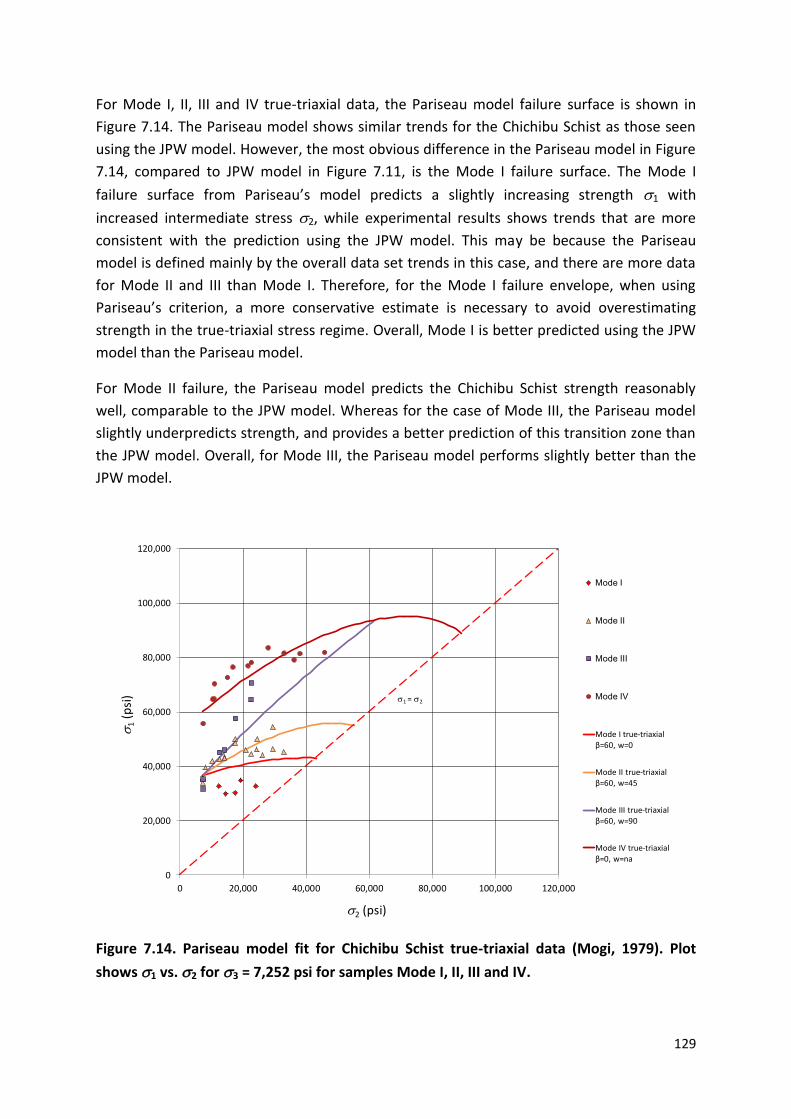
129
For Mode I, II, III and IV true-triaxial data, the Pariseau model failure surface is shown in
Figure 7.14. The Pariseau model shows similar trends for the Chichibu Schist as those seen
using the JPW model. However, the most obvious difference in the Pariseau model in Figure
7.14, compared to JPW model in Figure 7.11, is the Mode I failure surface. The Mode I
failure surface from Pariseau’s model predicts a slightly increasing strength 1 with
increased intermediate stress 2, while experimental results shows trends that are more
consistent with the prediction using the JPW model. This may be because the Pariseau
model is defined mainly by the overall data set trends in this case, and there are more data
for Mode II and III than Mode I. Therefore, for the Mode I failure envelope, when using
Pariseau’s criterion, a more conservative estimate is necessary to avoid overestimating
strength in the true-triaxial stress regime. Overall, Mode I is better predicted using the JPW
model than the Pariseau model.
For Mode II failure, the Pariseau model predicts the Chichibu Schist strength reasonably
well, comparable to the JPW model. Whereas for the case of Mode III, the Pariseau model
slightly underpredicts strength, and provides a better prediction of this transition zone than
the JPW model. Overall, for Mode III, the Pariseau model performs slightly better than the
JPW model.
Figure 7.14. Pariseau model fit for Chichibu Schist true-triaxial data (Mogi, 1979). Plot
shows 1 vs. 2 for 3 = 7,252 psi for samples Mode I, II, III and IV.
0
20,000
40,000
60,000
80,000
100,000
120,000
0 20,000 40,000 60,000 80,000 100,000 120,000
1
(psi
)
2 (psi)
Mode I
Mode II
Mode III
Mode IV
Mode I true-triaxialβ=60, w=0
Mode II true-triaxialβ=60, w=45
Mode III true-triaxialβ=60, w=90
Mode IV true-triaxialβ=0, w=na
1 = 2
Mogi Chichibu Schist (3D Pariseau model)
1 vs 2 ; 3 = 7,251 psi ; 2 > 3

130
For the case of intact rock failure in Mode IV, the Pariseau model prediction is only slightly
higher than the strengths predicted by the JPW model. Referring to Figure 7.14, the strength
prediction in the 1 > 90,000 psi stress regime indicates a reduced 2 strength effect. Due to
lack of experimental data at the higher strength 1 stress regime, the 2 effect at this higher
stress regime is derived based on the trends of 1 < 90,000 psi. To constrain the failure
envelope dependence on 2 at the higher stress level, an extension experiment where 1 =
2 for Mode IV would have been useful. This could provide better information regarding the
1 dependence at higher levels of 2. For the Chichibu Schist, most of the data are at stress
levels of 2 < 40,000 psi. Therefore, rock strength behavior at the lower 2 stress regime is
being used to predict the strength response at the higher 2 stress regime. This may not be
fully representative of the rock strength behavior at the higher 2 stress regimes. Instead,
the Pariseau model prediction could be improved if triaxial extension experiments were
available to constrain the 2 effect in the higher 2 stress regime.
The Pariseau model mean errors measured using the RMSE (see section 6.2 for the
definition of RMSE) for Chichibu Schist is 5,389 psi, which is slightly lower than that
determined for the JPW model, which gives an RMSE of 5,416 psi. Overall, it can be
concluded that both the Pariseau and JPW models predict the true-triaxial strength behavior
of the Chichibu Schist equally well.
7.7 Bossier shale calibration of JPW and Pariseau models using compression and extension
data
In this chapter, the JPW and Pariseau models were validated using the Chichibu Schist true-
triaxial experimental data. Both models were shown to be able to represent the strength
behavior in the true-triaxial stress regime equally well. However, the true-triaxial
experiments used for the Chichibu Schist are still not a common practice for industry
applications, and are largely used only for research purposes. Apart from that, cost and
equipment availability are the other issues that makes it impractical to make true-triaxial
experiments. For this reason, it would be very useful if JPW and Pariseau models
calibrations were made using only conventional triaxial experimental data.
Conventional triaxial equipment, which is standard rock testing equipment, can be used to
test the strength behavior under compressive loading conditions 1 > 2 = 3, and extension
loading conditions 1 = 2 > 3. Using the rock strength behavior at these stress conditions
may be sufficient to calibrate the models in the true-triaxial stress regime 1 > 2 > 3. In
this section, the compression and extension data for the shale samples will be used to
determine if these data are sufficient to calibrate both JPW and Pariseau models in the true-
triaxial stress regime.

131
For the Bossier shale, thirty-six triaxial compression tests were made under various
orientations and confining stresses for failure along the weak plane and intact rock.
However, for the Bossier shale triaxial extension tests, only five experiments were made for
failure along the weak plane. Therefore, for the Bossier shale samples in this study, the
conventional triaxial compression data were used to obtain the intact rock and weak plane
strength properties (i.e., o, So, w and Sw). These strength properties were then applied in
the true-triaxial stress regime to predict the triaxial extension strengths, and compare them
to experimental results at extensional stress conditions 1 = 2 = 25,000 psi and 3 = 7,190
psi (section 5.4 for Bossier shale sample shows extension tests at = 60o).
Figure 7.15a shows the JPW model for Mode I, II, III and IV in the true-triaxial stress regime,
as predicted using triaxial compression strength properties. Mode IV for intact rock strength
shows that triaxial compression and extension strengths are almost the same, with a slight
2 strength effect at intermediate stress levels. The JPW model Mode II and III predictions
shows a more pronounced 2 effect. However, there are no extension data available at
these Modes, and therefore this effect cannot be verified with experimental data.
For the Mode I condition, extension test data was compared with the JPW model that was
calibrated using conventional triaxial experimental data. The purpose of this exercise is to
evaluate whether or not the extension strength could be predicted using the JPW model
calibrated using strength properties from compression data. Figure 7.15a shows that the
JPW model Mode I prediction is slightly higher than the triaxial extension strength obtained
from experimental data at = 60o; 1 = 2 = 25,000 psi and 3 = 7,190 psi.
For the Pariseau model, triaxial compression and extension data were needed to calibrate
the model. These parameters were then applied in the true-triaxial stress regime to predict
the triaxial extension strength of the sample at = 60o, 1 = 2 = 25,000 psi and 3 = 7,190
psi. Figure 7.15b shows the failure modes I, II, III and IV predicted using Pariseau’s model.
The Pariseau model Mode IV shows that true-triaxial failure surface shows a significant 2
effect. This is because there are no extension data available for the intact rock failure under
Mode IV to sufficiently constrain the 2 effect. Alternatively, by introducing the intact rock
strength data in the triaxial extension stress regime, the 2 effect could be reduced,
resulting in a more constrained failure envelope, as that seen in Mode IV of Figure 7.15a for
the JPW model.
The plots in Figure 7.15a and 7.15b for Bossier shale in the true-triaxial stress regime show
that using triaxial compression data to predict extension strength could serve as an
approximate approach to determine the true-triaxial behavior of the Bossier shale.
However, due to lack of extension data for intact Mode IV rock failure, the true-triaxial
strength behavior for intact rock shows a low 2 effect for the JPW model, and a high 2
effect for the Pariseau model. Therefore, extension data of the intact rock are necessary in
order to calibrate the JPW and Pariseau models in the true-triaxial stress regime.

132
Figure 7.15a. JPW model fit for Bossier shale derived using strength parameters from
triaxial compression data. Plot shows 1 vs. 2 for 3 = 7,190 psi for samples Mode I, II, III
and IV.
Figure 7.15b. Pariseau model fit for Bossier shale derived using strength parameters from
triaxial compression and extension data. Plot shows 1 vs. 2 for 3 = 7,190 psi for samples
Mode I, II, III and IV.
0
5,000
10,000
15,000
20,000
25,000
30,000
35,000
40,000
45,000
50,000
0 5,000 10,000 15,000 20,000 25,000 30,000 35,000 40,000 45,000 50,000
σ1
(psi
)
σ2 (psi)
Joseph Bolan (3D Jaeger PoW) σ1 vs σ2 ; σ3=7,190 psi; σ2 > σ3
Triaxial extension
Mode I
Mode II
Mode III
Mode IV
Linear (Extension line)
33878.31 7000 24868.85 7000 24809.08 7000
34271.08 7500 25049.14 7500 25146.06 7500
use normal convention 34656.18 8000 25222.87 8000 25474.56 8000
Only make l = 90- 35033.7 8500 25390.12 8500 25794.71 8500
35403.73 9000 25550.93 9000 26106.59 9000
35766.36 9500 25705.37 9500 26410.29 9500
β σ1 σ3 36121.66 10000 25853.46 10000 26705.87 10000
90 6,140 0 36469.69 10500 25995.25 10500 26993.39 10500
60 1,811 0 36810.52 11000 26130.76 11000 27272.89 11000
45 6,874 0 37144.19 11500 26260.01 11500 27544.4 11500
45 5,653 0 37470.75 12000 26383.01 12000 27807.94 12000
30 6,577 0 37790.24 12500 26499.77 12500 28063.52 12500
0 16,466 0 38102.69 13000 26610.27 13000 28311.12 13000
Input to 3D
Pariseau
Input to 3D Pariseau
Mathlab
Input to 3D Pariseau
Mathlab
b=0; w=90 or 0 b=60; w=0 b=60; w=45
Mode IV Mode I Mode II
0
5,000
10,000
15,000
20,000
25,000
30,000
35,000
40,000
45,000
50,000
0 5,000 10,000 15,000 20,000 25,000 30,000 35,000 40,000 45,000 50,000
σ1
(psi
)
σ2 (psi)
Joseph Bolan (3D Pariseau) σ1 vs σ2 ; σ3=7,190 psi; σ2 > σ3
Triaxial extension
Mode I
Mode II
Mode III
Mode IV
Linear (Extension line)

133
7.8 Vaca Muerta shale calibration of JPW and Pariseau models using compression and
extension data
For the Vaca Muerta shale, twenty-one triaxial compression tests were conducted at
different orientations and confining stresses. For the triaxial extension tests, only two
experiments were successfully made for the intact rock fracture and failure along the weak
plane. For the Vaca Muerta triaxial extension tests of intact rock failure (section 5.4),
comparison of the compression and extension strengths show that the extension test for
intact rock strength is higher than the triaxial compressive strength. Using the Vaca Muerta
intact rock extension test data, the extension strength properties is estimated to be o =
37.6o and So = 3,805.1 psi, which are higher than the triaxial compression strength
parameters. This means that there is a significant 2 effect for the Vaca Muerta intact rock
strength. On the other hand, for failure along the weak plane, the Vaca Muerta Mohr circles
for triaxial compression and extension (section 5.4) show almost the same diameter,
indicating that the strength in compression and extension are the same. Based on this
observation, the strength parameter for failure along the weak plane are assumed to be w
= 26.0o and Sw = 2650 psi.
The JPW model for intact rock and weak plane failure applied in the true-triaxial stress
regime is shown in Figure 7.16a. The JPW model Mode IV intact rock failure envelope
predicts the strength at 1 = 2 = 25,000 psi and 3 = 1,150 psi, showing a significant 2
effect. The 1 strength under triaxial extension conditions is approximately 5,000 psi higher
than in triaxial compression. For modes I, II, and III, the failure envelopes are derived using
the weak plane strength properties. For failure along the weak plane, the Mode I failure
envelope shows an initially reducing 2 effect, which increases again when approaching 1 =
2, before asymptoting along the extension line. The JPW Mode II and Mode III failure
envelope shows higher 2 effects with increased direction .
For the Pariseau model, all the Vaca Muerta shale triaxial compression and extension data
were used to calibrate the model in the true-triaxial stress regime shown in Figure 7.16b.
Comparing the Pariseau model failure envelope to extension data shows that the Mode IV
failure envelope slightly overestimates 1 strength for triaxial extension strength by 2,000
psi. This is reasonable, considering that only one triaxial extension data is available for intact
rock failure. For failure along the weak plane, however, the Mode I failure envelope shows
an insignificant role of 2, while Mode II and III failure envelope shows stronger 2 effect.
For the Pariseau Mode IV failure envelope, the model prediction could be improved by
applying further constrains in calibrating the parameters in the true-triaxial stress regime.

134
Figure 7.16a. JPW model for Vaca Muerta shale using strength parameters from triaxial
compression and extension data. Plot shows 1 vs. 2 for 3 = 1,150 psi for Mode I, II, III
and IV.
Figure 7.16b. Pariseau model for Vaca Muerta shale using strength parameters from
triaxial compression and extension data. Plot shows 1 vs. 2 for 3 = 1,150 psi for Mode I,
II, III and IV.
Triaxial EXTENSION
0
0
5,000
10,000
15,000
20,000
25,000
30,000
0 5,000 10,000 15,000 20,000 25,000 30,000
σ1
(psi
)
σ2 (psi)
Vaca Muerta (3D Jaeger PoW) σ1 vs σ2 ; σ3=1,150 psi; σ2 > σ3
Triaxial extension
Mode I
Mode II
Mode III
Mode IV
Linear (Extension line)
1150 1450 1750 2050 2350 2650 2950 3250 3550
13706.58068 14007.44737 14305.2 14599.89093 14891.56 15180.26 15466.02432 15748.8886 16028.888
use normal convention Mode IV Mode I Mode II
Only make l = 90- 3D Pariseau 3D Pariseau 3D Pariseau
b=0; w=0 b=60; w=0 b=60; w=45
18295.79094 1150 13706.58068 1150 13706.58068 1150
β σ1 σ3 18587.76698 1450 13803.68403 1450 13905.08989 1450
60 7,874 0 18875.09722 1750 13897.64042 1750 14099.52413 1750
0 13,730 0 19157.86468 2050 13988.46653 2050 14289.92527 2050
19436.14666 2350 14076.17626 2350 14476.33015 2350
19710.01517 2650 14160.78074 2650 14658.77085 2650
19979.53722 2950 14242.28838 2950 14837.27481 2950
20244.77511 3250 14320.70496 3250 15011.86503 3250
20505.78675 3550 14396.03359 3550 15182.56018 3550
β σ1 σ3 20762.62587 3850 14468.27476 3850 15349.37469 3850
90 19,075 1,00021015.34222 4150 14537.42632 4150 15512.31883 4150
60 12,335 1,000 21263.98183 4450 14603.48351 4450 15671.39879 4450
0 20,120 1,000 21508.58714 4750 14666.43889 4750 15826.61667 4750
21749.19719 5050 14726.28234 5050 15977.97051 5050
21985.84772 5350 14783.001 5350 16125.45432 5350
22218.57138 5650 14836.57923 5650 16269.05796 5650
β σ1 σ3 22447.39778 5950 14886.99853 5950 16408.76716 5950
90 21,845 2,500 22672.35362 6250 14934.23746 6250 16544.56345 6250
75 19,935 2,500 22893.46277 6550 14978.27154 6550 16676.42398 6550
50 17,010 2,500 23110.74638 6850 15019.07316 6850 16804.32147 6850
40 18,005 2,500 23324.22292 7150 15056.6114 7150 16928.22406 7150
30 20,535 2,500 23533.90827 7450 15090.85194 7450 17048.09506 7450
20 21,950 2,500 23739.81574 7750 15121.75686 7750 17163.89284 7750
15 20,105 2,500 23941.95615 8050 15149.28447 8050 17275.57049 8050
24140.33783 8350 15173.38907 8350 17383.07561 8350
24334.96668 8650 15194.02074 8650 17486.34995 8650
24525.84616 8950 15211.12505 8950 17585.32907 8950
β σ1 σ3 24712.97734 9250 15224.64278 9250 17679.94188 9250
90 27,675 5,000 24896.35884 9550 15234.50954 9550 17770.11021 9550
80 33,640 5,000 Triaxial EXTENSION 25075.98689 9850 15240.65542 9850 17855.74825 9850
0
5,000
10,000
15,000
20,000
25,000
30,000
0 5,000 10,000 15,000 20,000 25,000 30,000
σ1
(psi
)
σ2 (psi)
Vaca Muerta (3D Pariseau) σ1 vs σ2 ; σ3=1,150 psi; σ2 > σ3
Triaxial extension
Mode I
Mode II
Mode III
Mode IV
Linear (Extension line)

135
In summary, comparing Figures 7.15a,b and 7.16a,b, the JPW and Pariseau models were
able to use compression and extension data to predict the true-triaxial strength behavior.
However, additional triaxial extension data (Mode I and IV) would significantly improve the
model calibration. In addition, using only compression and extension test data, the
intermediate stress levels in between compression and extension may not be properly
captured by the models, leading to failure envelopes that do not correctly represent the
actual true-triaxial failure behavior of the rock. Therefore, for JPW and Pariseau models,
true-triaxial experiments are still recommended, while more studies need to be done on
using compression and extension data for calibrating true-triaxial failure models.

136
8 Summary, Conclusions and
Recommendations
8.1 Summary and conclusions
In this chapter, the summary and conclusions of this thesis are described based on the
materials presented from the literature review, the experiments, the JPW and Pariseau
models, and finally the true-triaxial failure criteria. Before summarizing the overall thesis, it
is probably best to start by emphasizing the importance of understanding that shales are
complex natural materials. Organic-rich shales are even more complex because of the
presence of organic matter in the shale fabric, with planes of weakness that significantly
alters its mechanical behavior. Therefore, it is only correct to say that the focus of this study,
although providing a glimpse into the role of organic matter on strength behavior of shales,
does not give a complete picture of the various different textural or compositional effects
that may influence shale strength. To use the JPW or Pariseau models for organic-rich
shales, the user must be able to understand the different failure modes that may exist for
different types of shales.
In the introductory chapter, a mental picture of shales was presented to distinguish shales
by the scale of their discontinuities, texture and composition. The rock matrix that is
composed of discontinuities filled by minerals and sediments forms shales with planes of
weakness. Two key aspects that control the mechanical behavior of shales are texture and
composition. The effect of texture and composition were highlighted using three types of
minerals found predominantly in shales, namely calcite, quartz and clay. Here, shales with
similar composition but different texture result in different shale types. Therefore, it is
important to highlight that discontinuities, texture and composition play a key role in
understanding the mechanical response of shales.
A literature review uncovered many anisotropic rock failure criteria, which is categorized
according to the Duveau et al. (1998) classification as mathematical, empirical or
discontinuous (Table 2.1). Within these three categories of failure criteria, the mathematical
models are not widely used in engineering practice due to their complexity and lack of
experimental validation. As for the empirical criteria, these criteria are mainly extensions of
the isotropic criteria that use various parameters from fitting experimental data, and are
easily modified from existing failure criteria. Lastly, for the discontinuous criteria, most of
these criteria are related to the Coulomb criterion, which combines the failure mechanisms
along the weak plane and intact rock. The relative ease of modifying the Coulomb criterion
for weak plane and intact rock with other empirical or mathematical criterion led various
other combinations for the discontinuous models. Among these many criteria, to date the

137
JPW criterion (discontinuous) is still the industry-preferred model that is commonly used for
anisotropic rocks. This is probably because the JPW criterion originates from the well-known
Coulomb criterion, which is widely used in the industry for isotropic rocks. In this study, the
JPW criterion was presented in detail and tested using data from laboratory and the
literature, which are presented in Chapter 5. As for the Pariseau criterion (mathematical),
although this approach has been available for more than forty years, few researchers have
attempted to apply it to laboratory data. Therefore, the Pariseau criterion was tested
extensively in this study, and the results were presented in Chapter 6.
The laboratory measurements carried out in this study provide a unique understanding of
the strength behavior of the highly anisotropic Bossier shale and poorly laminated Vaca
Muerta Shale. The extensive experiments made on these organic-rich shales were described
in as much detail as possible, so that future studies could benefit from the lessons learned in
this study. An equally important finding from the experiments is that the quality control of
the experiments is paramount for ensuring good results. This is especially important, since
many experimental data are tested and analyzed, and all the data interpreted must be
consistent and as accurate as possible. Any gap or error in the processes used from sample
selection and interpretation would be difficult to correct because retesting or getting a
replacement sample is usually costly or in many cases not possible. Once all the quality
control measures from sample preparations up to data interpretation are followed, the
analysis is straightforward, with fewer uncertainties.
The Bossier shale and Vaca Muerta shale compressive strength tests show that strength
increases at higher confining stress. The compression tests also show that strength is
maximum at bedding angles = 0o and 90o, while the lowest strength was observed for the
samples tested at angle = 60o. The highly laminated Bossier shale showed higher strength
anisotropy compared to the poorly laminated Vaca Muerta shale. Another important
observation from the experimental results is that the UCS strength at angle = 90o is much
lower than at = 0o, which means that UCS values are not representative of the shale
strength behavior under non-zero confining stress. This also means that the Bossier shale
UCS data should not be used for design of wellbore stability analysis. The same condition
could not be verified for the Vaca Muerta shale, due to lack of data at = 90o, but the issue
of unconfined strength is suspected to occur only for highly anisotropic shales such as the
Bossier shale, due to tensile splitting at low confining stresses. Low strength anisotropy
shale such as the Vaca Muerta did not show any tensile splitting behavior at angle = 90o.
Five extension tests were performed for the Bossier shale, while for Vaca Muerta shale only
two extension tests were conducted. All of the extension tests were for failure along the
weak plane, except for one Vaca Muerta sample that was tested for intact rock failure.
Results show that for weak plane failure, there is no significant difference in strength
between the triaxial compression and triaxial extension tests. However, a significant
difference was found between the Vaca Muerta compression and extension tests for intact

138
rock failure. This means that the 2 effect is not significant for failure along the weak plane,
whereas for the intact rock failure the 2 effect is important and cannot be ignored.
However, these experiments do not address the complete true-triaxial stress condition,
which also includes the direction, .
Although the main focus of this study was on strength behavior, the elastic behavior of the
anisotropic shales was very useful as a measure of quality control. For the highly anisotropic
Bossier shale, the Young’s modulus and Poisson’s ratio data showed S-shaped behavior
consistent with the theoretical predictions. However, for the Vaca Muerta shale, although
the theoretical curve shows a similar S-shape, the experimental data shows significant
scatter due to possible sample heterogeneity and competition of isotropic-anisotropic
elastic behavior. This means that some of the Vaca Muerta samples tested behaved in a
transition manner and showed more elastic isotropy and less elastic anisotropic behavior.
Another observation for both the shales tested was that confining pressure affected the
elastic moduli. The Bossier shale elastic moduli increased at higher confining pressures,
whereas for Vaca Muerta shale, this effect of pressure on the elastic moduli was not
detectable, due to significant scatter in the data.
Using CT scans and thin section images, two types of shale fabric were evaluated in this
study. The first is the Bossier shale, which is highly laminated with discontinuous weak
planes, wherein the planes are filled with organic material. The second shale evaluated was
the Vaca Muerta shale, which is slightly different from the Bossier shale, wherein the fabric
arrangement shows poor lamination, and the organic matter is dispersed throughout the
shale matrix. Evaluations of the CT and thin-section images show that the fabric of the
organic matter affects the failure modes and strength behavior of shales. For the Bossier
shale, both CT and thin section images were necessary to evaluate the shale fabric.
However, for the Vaca Muerta shale, the CT scan images provided better information than
the thin section images regarding the failure modes.
Comparison of the Bossier shale pre-test and post-test thin section images shows that for
samples with bedding angles = 0o to 10o and = 90o, failure occurs at a fracture plane
angle consistent with the Coulomb criterion. At angles between 45o < < 75o, the samples
failed predominantly along the weak planes, also consistent with the Coulomb criterion.
However, there is a transition regime of angles lying in the range of about 10o < < 35o,
wherein the failure surface follows an irregular path, and shows a mixed failure mode of
intact rock fracture and weak plane failure. The transition zone with mixed failure modes for
the Bossier shale is a new observation, and was further examined using thin section images.
Thin section images at angles = 15o to 30o show that the sample failure plane occurs
through the intact rock or weak plane lamination, jumping between the two failure modes
with a step-like pattern, wherein the weak planes interact with the matrix shear fractures,
following the path of least resistance. One possible explanation for this behavior is that at
the transition zone, the discontinuous weak planes intersect the shale matrix failure plane,

139
providing an alternative fracture path, resulting in shale strength that is lower than the
matrix rock strength. This mixed-failure mode due to competition of shale matrix and weak
planes is caused by uneven distribution of high stresses at the transition zone, resulting in
shale failure at lower strength than the JPW model prediction. The mixed-failure mode also
causes the transition from shear fracture to sliding on a weak plane to occur over a range of
angles < 1 and > 2, rather than exclusively at 1 and 2, as predicted by the JPW
model.
For the Vaca Muerta shale, a comparison of the pre-test and post-test CT scan images does
not show the presence of a transition zone or mixed failure modes, as was observed for the
Bossier shale. All of the compressive test samples failed in shear through the matrix, or
along a weak plane, in agreement with the JPW model predictions. The failure surfaces and
weak plane laminations were also more easily observed using the CT scan images than in
the thin section images.
Although the JPW model is already well known in the industry, it is difficult to find in the
literature a clear explanation of how this model is derived from the Coulomb criterion. This
was described in detail by deriving the JPW model using the Coulomb criterion equations
and Mohr’s circle. The definition of angle was also discussed in detail, to show that the
same Coulomb criterion is applicable in compression and extension conditions.
The Pariseau continuum model was the other criterion that was described in detail. Both the
JPW and Pariseau models for triaxial compression and extension condition were then fit for
the Bossier shale and Vaca Muerta shales tested in this study. Comparing both models,
Pariseau’s model gives a better fit to the Bossier shale data than does the JPW model, with a
RMSE of 3,248 psi, as compared with 4,171 psi for the JPW model. The difference in
accuracy between the two models is mainly caused by the different model predictions in the
transition zone 10o < < 35o, where the JPW model overestimates strength. For the Vaca
Muerta shale, the Pariseau model provided a poorer fit than did the JPW model, with an
RMSE of 2,390 psi, compared with the JPW model’s RMSE of 1,851 psi. The Vaca Muerta
shale exhibited a nearly uniform strength in the range of angles 0o < < 40o, and did not
show any transition zone; its behavior was therefore more consistent with the assumptions
of the JPW model. In summary, both the JPW and Pariseau models show a reasonable ability
to fit strength data on the Bossier and Vaca Muerta shales. The Bossier shale was a better fit
with the Pariseau model, having an RMSE error smaller by 28%, whereas the JPW model
gave a better fit to the Vaca Muerta shale, with an RMSE error smaller by 29%.
To distinguish the different anisotropic rock types, a method to determine the strength
anisotropy ratio (SAR) was proposed, which can be expressed in terms of the fitting
parameters of the JPW model as follows:
(
) (
) (8.1)

140
The JPW and Pariseau models were then applied to the ten data sets from the literature,
and the two shales tested in this study. The best-fit model with the least RMSE for each
anisotropic rock type was calculated, and is displayed in a bar chart shown in Figure 8.1.
Each column shows the RMSE for both the Pariseau and JPW model, along with the SAR
value derived from the JPW fit.
Figure 8.1. Comparison of JPW and Pariseau models for various anisotropic rocks.
* denotes data from the present study.
Comparison of the RMSE for all the rock types shows that the Pariseau model provides a
better fit for ten of the twelve rocks, whereas the JPW model provided a better fit only for
the Vaca Muerta shale (SAR = 1.87) and the Green River Shale-1 (SAR = 1.52). It can be
noted that all rocks with SAR > 2 fit more closely by the Pariseau model, whereas both
shales that were a better fit with the JPW model had SAR < 2. Nevertheless, three rocks with
SAR < 2 fit more accurately by the Pariseau model; therefore, it seems that no definitive
conclusions can be reached in this regard.
Using the available data from experiments and the literature, the JPW and Pariseau models
were also evaluated using reduced data to determine the minimum number of triaxial
experiments necessary to determine the strength parameters without significantly lowering
the model accuracy. Evaluations of both models show that the Pariseau model gives a lower
Bo
ssie
r s
ha
le *
Vac
a M
uer
ta s
hal
e *
An
gers
Sch
ist
Ma
rtin
sbu
rg S
late
Au
stin
Sla
te
Gre
enR
iver
Sh
ale
-1
Gre
enR
iver
Sh
ale
-2
Qu
art
z P
hyl
lite
Ca
rbo
na
Ph
yllit
e
Mic
ace
ou
s P
hyl
lite
Pen
rhyn
Sla
te
Tou
rnem
ire
Sh
ale
0
1,000
2,000
3,000
4,000
5,000
6,000
7,000
0
1,000
2,000
3,000
4,000
5,000
6,000
7,000
RM
SE (p
si)
Anisotropic rock types
JPW RMSE(psi)
Pariseau RMSE(psi)
SAR
= 1
.87
SAR
= 6
.21
SAR
= 4
.84
SAR
= 2
.10
SAR
= 1
.52
SAR
= 1
.60 SA
R =
1.7
5
SAR
= 1
.93
SAR
= 3
.08
SAR
= 2
.10
SAR
= 1
.57
SAR
= 2
.02

141
RMSE than the JPW model, when evaluated using reduced number of data. The Pariseau
model analysis shows that eight data points, obtained at two confining stress levels and at
bedding angles = 0o, 30o, 60o and 90o, is the recommended minimum data needed for
using Pariseau’s model. This recommendation of minimum numbers of data is also
applicable using JPW models for rocks with low SAR. For the analysis of anisotropic rocks
with high SAR, the JPW model analysis using minimum number of data set will need at least
fourteen triaxial compression data at bedding angles of = 0o, 15o, 30o, 45o, 60o 75o and 90o
at two confining stress levels.
A good understanding of the JPW and Pariseau models was gained from the experimental
work for the Bossier shale and Vaca Muerta shale, and applying these two models for
various anisotropic rocks gave further insight into both models. The experience from using
the JPW and Pariseau models in Chapter 5 and 6, under conventional triaxial stress
conditions, provided the right understanding for applying the same models for true-triaxial
stress conditions. The JPW and Pariseau failure criteria for true-triaxial stress conditions
were described in Chapter 7, and validated using the Chichibu Schist data set published by
Mogi (1979). The Chichibu Schist true-triaxial data fit using the JPW model gave an RMSE of
5,416 psi, whereas the Pariseau model produced an RMSE of 5,389 psi. Overall, it can be
concluded that both Pariseau and JPW models predict the true-triaxial strength behavior of
the Chichibu Schist equally well. An interesting observation from the Mode I true-triaxial
experiments show that 2 decreases initially before increasing, which is an interesting and
unexpected phenomenon for the 2 effect. This reduced strength 1 with increased 2 is a
new response discovered in this study, and the true-triaxial JPW model captures this
behavior. All the Chichibu Schist samples tested under true-triaxial stress conditions with
Mode I, II, III and IV show that strength 1 depends not only on confining pressure 3,
intermediate stress 2 and angle , but also is significantly influenced by the direction
(direction is the angle of the foliation with respect to the direction of the intermediate
principal stress, 2).
8.2 Recommendations
Two types of organic-rich shales, one highly laminated and one poorly laminated, were
tested in this study. The fabric of the organic matter plays a key role in the failure mode of
both shales, as was discovered in this study. The highly laminated Bossier shale with
organic-filled weak planes shows a mixed failure mode, while the dispersed organic matter
in the Vaca Muerta shale with poor laminations showed smaller discrepancies with the
predictions of the JPW model. Further experiments for different types of organic-rich shales
are therefore recommended to uncover other potential failure modes and improve the
model predictions.
142
The Bossier shale and Vaca Muerta shale were tested under conventional triaxial
compression or extension conditions. However, the actual strength behavior of shales under
true-triaxial stress conditions remains untested. Although the JPW and Pariseau true-triaxial
models were validated in this study for the Chichibu Schist, failure behavior of organic-rich
shales under true-triaxial stress condition could be different due to the presence of organic
matter. The influence of the transition zone, organic-filled weak planes and fracture
direction and angle for true-triaxial experiments needs to be further evaluated. Other
failure modes under true-triaxial stress condition, similar to the transition zone for the
Bossier shales, remain to be discovered.
During the triaxial extension experiments, some end effects were observed on the Bossier
shale and Vaca Muerta shales samples, which causes problems in interpreting the results.
For future experiments on organic-rich shales, further studies need to be made to
determine if a different sample dimensions are necessary (i.e., height ratio, smaller sample,
larger samples, etc.) to reduce possible end effect such as that seen for the Vaca Muerta
sample at = 90o. Further evaluations also need to be made to determine if the extension
tests could be affected due to high friction at the contact point between the axial loading
ram and the sample. Improvement in the design of the endcap contact points between
sample and axial loading ram should also be considered.
In view of possible applications on the findings from this study, the JPW and Pariseau
models are recommended to be applied to wellbore stability analysis using actual field data.
To determine the stresses around the wellbore, the anisotropic rock elastic model should be
used to have a better estimate of the near wellbore stresses. Obtaining such field data to be
tested is a time consuming process and needs careful planning and investment. A single case
study may not give clear results, and tests should be done for several wells to have
meaningful results.
In the study of shale fabric analysis, one of the most pertinent questions in the industry is
the relationship, if any, between texture and composition and mechanical behavior.
Textural and compositional information used in the industry quantitatively define shale
petrology for geological characterization. Quantitative geology (i.e., TOC, porosity, density,
volume, etc.) is useful for identification and classification purposes, but has limited use for
determining mechanical behavior. Sone and Zoback (2013a, b) provided equations relating
shale properties such as clay % (vol.), carbonate % (vol.), kerogen % (vol.) and bulk density,
to mechanical properties such as creep, strength and elastic moduli. However, the amounts
of scatter in these relationships are significant and in some cases, there are no clear trends
observed.
For estimating strength properties from the shale fabric, one area that could be explored is
the use of X-Ray technology such as CT (Computed Tomography) scans. In recent years, CT
scans have become standard equipment used in the industry to characterize the internal
features of the rock. Although CT scans provide bulk density quantitatively, most of the

143
textural features are determined qualitatively. Therefore, the use of texture and
composition to determine rock strength is an issue that may not be solved using existing CT
technology. Further development is necessary to measure the shale fabric quantitatively,
and applying additional analysis for estimating strength behavior.
Improvement in CT technology to capture the textural features of the shale fabric needs to
be complemented by further development of digital analysis and numerical methods.
Textural features of the shale fabric captures the actual discontinuities and flaws that exist
in the rock, which is an improvement from the idealized analytical models used in this study.
The advantage of numerical methods is the ability to model complex features in the rock,
which is a limitation for analytical models described in this study. Capturing the actual
textural features in shale fabric and analyzing the rock behavior using numerical simulation
still needs to be supplemented with experimental data that accounts for both textural and
compositional effects. Numerical methods using CT technology and experimental data can
then be used to determine the mechanical behavior of very complex shales, which could
then lead to complete analysis under true-triaxial stress conditions for highly anisotropic
shales. This is an exciting area of research with tremendous potential for future applications.

144
References
Aadnoy, B.S., 1988. Modelling of the stability of highly inclined boreholes in anisotropic rock formations. SPE Drilling Engineering, Vol. 3, p. 259-268.
Aadnoy, B.S., Hareland, G, Kustamsi, A., de Freitas, T., and Hayes, J., 2009. Borehole failure related to bedding plane. In: Proceedings of the 43th US Rock Mechanics Symposium, 28 June – 1 July 2009, Asheville, N. Carolina, paper ARMA 09-106.
Al-Ajmi, A.M. and Zimmerman, R.W., 2005. Relation between the Mogi and the Coulomb failure criteria. Int. J. Rock Mech. Min. Sci., Vol. 42, p. 431-439.
Al-Ajmi, A.M. and Zimmerman, R.W., 2006. Stability analysis of vertical boreholes using the Mogi-Coulomb failure criterion. Int. J. Rock Mech. Min. Sci., Vol. 43, p. 1200-1211.
Allirot, D., Boehler, J.P. and Sawczuk, A., 1977. Irreversible deformations of an anisotropic rock under hydrostatic pressure. Int. J. Rock Mech. Min. Sci., Vol. 14, p. 77-83
Amadei, B., 1983. Rock anisotropy and the theory of stress measurements. (Lecture notes in engineering 2), Springer, Heidelberg.
Amadei, B., 1996. Importance of anisotropy when estimating and measuring in situ stresses in rock. Int. J. Rock Mech. Min. Sci., Vol. 33, no. 3, p. 293-325.
Ashour, H.A., 1988. A compressive strength criterion for anisotropic rock materials. Eng. J. Qatar Univ., Vol. 1, p. 11-21.
Attewell, P.B., and Sandford, M.R., 1974. Intrinsic shear strength of a brittle, anisotropic rock – Part 1. Experimental and mechanical interpretation. Int. J. Rock Mech. Min. Sci., Vol. 11, p. 423-430.
Baker, Jr. E.T., 1995. Stratigraphic Nomenclature and Geological Sections of the Gulf Coastal Plain of Texas. US Geological Survey (Open file report 94-461), Austin, Texas.
Barton, N. and Choubey, V., 1977. The shear strength of rock joints in theory and practice. Rock Mech., Vol. 10, p. 1-54.
Brace, W.F., 1965. Relation of elastic properties of rock to fabric. J. Geophys. Res., Vol. 70, No. 22, p. 5657-5667.
Brady, B.H.G. and Brown, E.T., 1993. Rock mechanics for underground mining. 2nd Ed., Chapman & Hall, London.
Budd, C.H., McLamore, R.T. and Gray, K.E., 1967. Microscopic examination of mechanically deformed oil shale. In: Annual Meeting of the American Institute of Mining, Metallurgical, and Petroleum Engineers, 1–4 October 1967, Houston, Texas, paper SPE 1826, p. 1-23.
Cazacu, O. and Cristescu, N.D., 1999. A paraboloid failure surface for transversely isotropic materials. J. Mech. Mater., Vol. 31, p. 381-393.

145
Chang, C., Zoback, M.D. and Khaksar, A., 2006. Empirical relation between rock strength and physical properties in sedimentary rocks. J. Pet. Sci. Eng., Vol. 51, Issues 3-4, p. 223-237.
Chenevert, M.E. and Gatlin, C., 1964. Mechanical anisotropies of laminated sedimentary rocks. In: Proceedings of the 39th Annual Fall Meeting, Oct. 11–14, Houston, Texas, paper SPE 890, p. 67-77.
Choo, J.W., Kim, H., Jeon, S. and Min, K.B., 2012. Deformation and strength anisotropy of Asan gneiss, Boryeong shale and Yeoncheon schist. Int. J. Rock Mech. Min. Sci., Vol. 50, p. 158-169.
Colmenares, L.B. and Zoback, M.D., 2002. A statistical evaluation of intact rock failure criteria constrained by polyaxial tests data for five different rocks. Int. J. Rock Mech. Min. Sci., Vol. 39, p. 695-729.
Cook, J.M., Goldsmith, G., Audibert, A.M., Bieber, M.T. and Jacqueline, L., 1993. Mud/Shale Interaction: model wellbore studies using x-ray tomography. In: SPE/IADC Drilling Conference, February 23-25, Houston, Texas, paper SPE/IADC 25729.
Corley, B. Garcia, A., Maurer, H.M., Rabinovich, M.B., Zhou, Z., DuBois, P. and Shaw Jr., N., 2010. Study of unusual responses from multiple resistivity tools in the Bossier formation of the Haynesville shale play. In: SPE Annual Technical Conference and Exhibition, 19–22 September 2010, Florence, Italy, paper SPE 134494.
Donath, F.A., 1961. Experimental study of shear failure in anisotropic rocks. Geol. Soc. America Bulletin, Vol. 72, p. 985-990.
Donath, F.A., 1964. Strength variation and deformational behavior of anisotropic rocks; State of Stress in the Earth's Crust. In : Proceedings of the International Conference, 13 June–14 June 1963, Santa Monica, Cal., p. 281-298.
Donath, F.A., Fruth, L.S. and Olsson, W.A., 1972. Experimental study of frictional properties of faults. In: Proceedings of the 14th U.S. Symposium on Rock Mechanics, 23–26 June 1972, University Park, Pennsylvania, paper ARMA 72-0189.
Drucker, D.C. and Prager, W., 1952. Soil mechanics and plastic analysis for limit design. Q. Appl. Math., Vol. 10, no. 2, p. 157-165.
Duveau, G., Shao, J.F. and Henry, J.P., 1998. Assessment of some failure criteria for strongly anisotropic geomaterials. Mech. Cohesive-Frictional Mater., Vol.3, p. 1-26.
Ewy, R.T., Bovberg, C.A. and Stankovic, R.J., 2010. Strength anisotropy of mudstones and shales. In: Proceedings of the 44th US Rock Mechanics Symposium, 27–30 June 2010, Salt Lake City, paper ARMA 10-114.
Fairhurst, C.E. and Hudson, J.A., 1999. ISRM suggested method for complete stress-strain curve for intact rock in uniaxial compression. Int. J. Rock Mech. Min. Sci., Vol. 36, p. 279-289.
Fjaer, E. and Nes, O.M., 2013. Strength anisotropy of Mancos shale. In: Proceedings of the 47th US Rock Mechanics Symposium, 23–26 June 2013, San Francisco, paper ARMA 13-519.
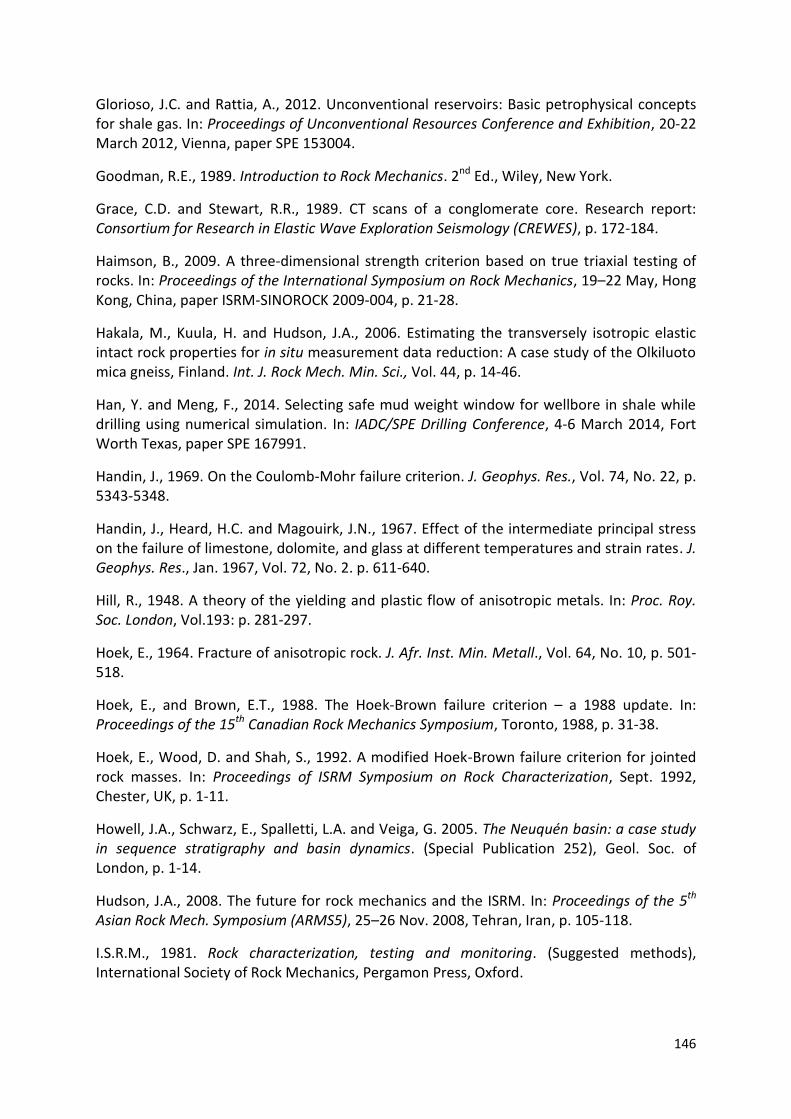
146
Glorioso, J.C. and Rattia, A., 2012. Unconventional reservoirs: Basic petrophysical concepts for shale gas. In: Proceedings of Unconventional Resources Conference and Exhibition, 20-22 March 2012, Vienna, paper SPE 153004.
Goodman, R.E., 1989. Introduction to Rock Mechanics. 2nd Ed., Wiley, New York.
Grace, C.D. and Stewart, R.R., 1989. CT scans of a conglomerate core. Research report: Consortium for Research in Elastic Wave Exploration Seismology (CREWES), p. 172-184.
Haimson, B., 2009. A three-dimensional strength criterion based on true triaxial testing of rocks. In: Proceedings of the International Symposium on Rock Mechanics, 19–22 May, Hong Kong, China, paper ISRM-SINOROCK 2009-004, p. 21-28.
Hakala, M., Kuula, H. and Hudson, J.A., 2006. Estimating the transversely isotropic elastic intact rock properties for in situ measurement data reduction: A case study of the Olkiluoto mica gneiss, Finland. Int. J. Rock Mech. Min. Sci., Vol. 44, p. 14-46.
Han, Y. and Meng, F., 2014. Selecting safe mud weight window for wellbore in shale while drilling using numerical simulation. In: IADC/SPE Drilling Conference, 4-6 March 2014, Fort Worth Texas, paper SPE 167991.
Handin, J., 1969. On the Coulomb-Mohr failure criterion. J. Geophys. Res., Vol. 74, No. 22, p. 5343-5348.
Handin, J., Heard, H.C. and Magouirk, J.N., 1967. Effect of the intermediate principal stress on the failure of limestone, dolomite, and glass at different temperatures and strain rates. J. Geophys. Res., Jan. 1967, Vol. 72, No. 2. p. 611-640.
Hill, R., 1948. A theory of the yielding and plastic flow of anisotropic metals. In: Proc. Roy. Soc. London, Vol.193: p. 281-297.
Hoek, E., 1964. Fracture of anisotropic rock. J. Afr. Inst. Min. Metall., Vol. 64, No. 10, p. 501-518.
Hoek, E., and Brown, E.T., 1988. The Hoek-Brown failure criterion – a 1988 update. In: Proceedings of the 15th Canadian Rock Mechanics Symposium, Toronto, 1988, p. 31-38.
Hoek, E., Wood, D. and Shah, S., 1992. A modified Hoek-Brown failure criterion for jointed rock masses. In: Proceedings of ISRM Symposium on Rock Characterization, Sept. 1992, Chester, UK, p. 1-11.
Howell, J.A., Schwarz, E., Spalletti, L.A. and Veiga, G. 2005. The Neuquén basin: a case study in sequence stratigraphy and basin dynamics. (Special Publication 252), Geol. Soc. of London, p. 1-14.
Hudson, J.A., 2008. The future for rock mechanics and the ISRM. In: Proceedings of the 5th Asian Rock Mech. Symposium (ARMS5), 25–26 Nov. 2008, Tehran, Iran, p. 105-118.
I.S.R.M., 1981. Rock characterization, testing and monitoring. (Suggested methods), International Society of Rock Mechanics, Pergamon Press, Oxford.

147
Islam, M.A., Skalle, P., Al-Ajmi, A.M. and Søreide, O.K., 2010. Stability analysis in shale through deviated boreholes using the Mohr and Mogi-Coulomb failure criteria. In: Proceedings of the 44th US Rock Mechanics Symposium, 27–30 June 2010, Salt Lake City,, paper ARMA 10-432.
Jaeger, J. C., Cook, N.G.W. and Zimmerman, R.W., 2007. Fundamentals of Rock Mechanics, 4th Ed. Blackwell, Oxford.
Jaeger, J.C. and Cook, N.G.W., 1976. Fundamentals of Rock Mechanics. 3rd Ed.Chapman & Hall, London.
Jaeger, J.C., 1960. Shear failure of anisotropic rock. Geol. Mag., Vol. 97 p. 65-72.
Jaeger, J.C., 1962. Elasticity, fracture and flow. 2nd Ed., Methuen, New York.
Jaeger, J.C., 1964. Elasticity, fracture and flow. 2nd Ed. (Reprinted with corrections), Barnes & Noble, New York.
Jaeger, J.C., 1966. Brittle fracture of rocks. In: Proceedings of the 8th US Rock Mechanics Symposium, 15–17 September, Minneapolis, paper ARMA 66-0003.
Jaeger, J.C., 1971. Friction of rocks and stability of rock slopes. Géotechnique 21, No. 2, p. 97-134.
Knopf, E.B., 1957. Petrofabrics in structural geology. In: Proceedings of the 2nd US Rock Mechanics Symposium, 21–24 April 1957, Golden, Colorado, paper ARMA 57-0099.
Kusabuka, M., Takeda, H. and Kojo, H., 1999. Anisotropic yield function for rocks and evaluation of material parameters. In: Proceedings 9th Int. Congress of Rock Mechanics, Paris, 25028 August, , p. 921-924.
Kwaśniewski, M. and Mogi, K., 1990. Effect of the intermediate principal stress on the failure of a foliated anisotropic rock. In: Proceedings of Int. Conf. Mech. Jointed and Faulted Rock, H.P. Rossmanith (Ed.), Balkema, Rotterdam, p. 407-416.
Kwaśniewski, M., 1993. Mechanical behavior of anisotropic rocks. Comprehensive rock engineering. Pergamon Press, Oxford, Vol. 1, p. 285-312.
Kwaśniewski, M., 2007. Mechanical behavior of rocks under true triaxial compression conditions – volumetric strain and dilatancy. Arch. Min. Sci., Vol. 52, No. 3, p. 409–435.
Lade, P.V., 1993. Rock strength criteria: The theories and the evidence. Comprehensive rock engineering. Pergamon Press, Oxford, Vol. 1, p. 255-284.
Lee, H., Ong, S.H., Azeemuddin, M. and Goodman, H., 2012a. A wellbore stability model for formation with anisotropic rock strengths. J. Pet. Sci. Eng., Vol. 96 – 97, p. 109 – 119.
Lee, K-Y. Pietruszczak, S. and Choi, B-H., 2012b. Failure criteria for rocks based on smooth approximations to Mohr-Coulomb and Hoek-Brown failure functions. Int. J. Rock Mech. Min. Sci., Vol. 56 , p. 146-160.

148
Lee, K-Y. and Pietruszczak, S., 2007. Application of critical plane approach to the prediction of strength anisotropy in transversely isotropic rock masses. Int. J. Rock Mech. Min. Sci., Vol. 45, p. 513-523.
Ma, X. and Haimson, B., 2012. True triaxial compression tests on a medium-high porosity sandstone and the effect of the intermediate principal stress on strength and fault angle. In: Proceedings of the 46th US Rock Mechanics Symposium, 24–27 June, Chicago, paper ARMA 2012-182.
McClintock, F.A. and Walsh, J.B., 1962. Friction on Griffith cracks in rocks under pressure. In: Proceedings of the 4th U.S. National Congress on Applied Mech. Berkeley, p. 1015-1021.
McLamore, R.T. and Gray, K.E., 1967. A strength criterion for anisotropic rocks based upon experimental observations. SPE Annual Meeting of the American Institute of Mining, Metallurgical, and Petroleum Engineers, 19–23 February 1967, Los Angeles, paper SPE 1721.
Meyer, J.P., Labuz, J.F. and Lin, Q., 2012. Intermediate stress effect in reverse: strength anisotropy. In: Proceedings of the 46th US Rock Mechanics / Geomechanics Symposium, 24–27 June 2012, Chicago, paper ARMA 12-561.
Mogi, K., 1967. Effect of intermediate principal stress on rock failure. J.Geophys. Res., Vol. 72, p. 5117-5130.
Mogi, K., 1971. Effect of the triaxial stress system on the failure of Dolomite and Limestone. Tectonophysics, Vol. 11, p. 111-127.
Mogi, K., 1972. Fracture and flow of rocks. Tectonophysics, 13 (1-4): p. 541-568.
Mogi, K., 1973. Rock fracture. Annual Rev. Earth Planet. Sci. Vol. 1, p.63-84.
Mogi, K., 1979. Flow and fracture of rocks under general triaxial compression. In: Proceedings of the 4th ISRM Congress, September 2–8, 1979, Montreux, Switzerland, p. 123-131.
Mogi, K., 2007. Experimental rock mechanics.Taylor & Francis. London.
Monreal, F.R., Villar, H.J., Baudino, R., Delpino, D. and Zencich, S., 2009. Modelling an atypical petroleum system: A case study of hydrocarbon generation, migration and accumulation related to igneous intrusions in the Neuquen Basin, Argentina. Mar. Pet. Geol., Vol. 26 p. 590-605.
Monti, L.J, Suarez, M.I., Antony, R. and Vega, L., 2013. Modelling vertical multifractured wells in Vaca Muerta shale oil play. In: Proceedings of the Unconventional Resources Conference, 10–12 April 2013, Woodlands, Texas, paper SPE 164537.
Mooney, C. Z., 1997. Monte Carlo Simulation. Series: Quantitative applications in the social sciences. Sage Publications, No. 07-116.
Mŕoz, Z. and Maciejewski, J., 2011. Critical plane approach to analysis of failure criteria for anisotropic geomaterials. Springer Series in Geomech. and Geoeng., p. 69-89.
Nadai, A., 1950. Theory of flow and fracture of solids, 2nd ed. McGraw-Hill, New York.

149
Narayanasamy, R., Barr, D and Milne, A., 2009. Wellbore instability predictions within the Cretaceous mudstones. In: SPE Offshore Europe Oil & Gas Conference & Exhibition, 8 – 11 September 2009, Aberdeen, UK, paper SPE 124464.
Nasseri, M.H.B., Rao, K.S. and Ramamurthy, T., 2003. Anisotropic strength and deformational behavior of Himalayan schists. Int. J. Rock Mech. Min. Sci., Vol. 40, Issue 1 p. 3-23.
Niandou, H. Shao, J.F., Henry, J.P. and Fourmaintraux, D., 1997. Laboratory investigation of the mechanical behaviour of Tournemire shale. Int. J. Rock Mech. Min. Sci., Vol. 34, Issue 1, Jan. 1997, p. 3-16.
Nova, R., 1980. The failure of transversely isotropic rocks in triaxial compression. Int. J. Rock
Mech. Min. Sci., Vol. 17, Issue 6, December 1980, p. 325–332.
Ong, S.H. and Roegiers, J-C., 1993. Horizontal wellbore collapse in an anisotropic formation. In: The Production Operations Symposium, 21–23 March 1993, Oklahoma City, Oklahoma, paper SPE 25504.
Pariseau, W.G., 1968. Plasticity theory for anisotropic rocks and soils. In: Proceedings of the 10th US Symposium on Rock Mechanics, 20-22 May, Austin, Texas, paper ARMA 68-0267.
Pariseau, W.G., 2012. A symmetry requirement for failure criteria. Int. J. Rock Mech. Min. Sci., Vol. 52 p. 46-49.
Pariseau, W.G., 2012b. Design Analysis in Rock Mechanics, 2nd Ed., Taylor & Francis, London.
Parry, R.H.G., 2000. Shear strength of geomaterials – A brief historical perspective. In: The ISRM International Symposium, November 19–24, 2000, Melbourne, Australia, paper ISRM-IS-2000-041.
Paterson, M.S., 1982. (BIOGRAPHICAL MEMOIRS), John Conrad Jaeger 1907-1979, http://science.org.au/fellows/memoirs/jaeger.html#1. Memoir originally published in Historical Records of Australian Science, vol.5, no.3, 1982.
Pei, J., 2008. Strength of transversely isotropic rocks. PhD Thesis, MIT.
Pietruszczak, S. and Mŕoz, Z., 2001. On failure criteria for anisotropic cohesive-frictional materials. Int. J. Anal. Geomech., 2001; 25: p. 509-524.
Ramamurthy, T. and Arora, V.K., 1994. Strength predictions for jointed rocks in confined and unconfined states. Int. J. Rock Mech. Min. Sci. & Geomech. Vol. 31, No.1, p. 9-22.
Ramamurthy, T., 1993. Strength and modulus response of anisotropic rocks. Comprehensive rock engineering. Pergamon Press, Oxford, Vol. 1, p. 313-329.
Ramamurthy, T., 2001. Shear strength response of some geological materials in triaxial compression. Int. J. Rock Mech. Min. Sci., Vol. 38, Issue 5 2001, p. 683-697.
Ramamurthy, T., Rao, G.V. and Singh, J., 1993. Engineering behavior of phyllites. Eng. Geol., Vol. 33, Issue 3, p. 209-225.

150
Reik, G. and Zakas, M., 1978. Strength and deformation characteristics of jointed media in true triaxial compression. Int. J. Rock Mech. Min. Sci. Vol. 15, p. 295-303.
Rushing, J.A., Newsham, K.E. and Blasingame, T.A., 2008. Rock typing – Keys to understanding productivity in tight gas sands. In: Proceedings of the Unconventional Reservoirs Conference, 10–12 February 2008, Keystone, Colorado, paper SPE 114164.
Santarelli, F.J., Zaho, S., Burrafato, G., Zausa, F. and Giacca, D., 1997. Wellbore-stability analysis made easy and practical. In: SPE/IADC Drilling Conference, 12–15 March 1996, New Orleans, paper SPE 35105.
Saroglou, H. and Tsiambaos, G., 2007a. A modified Hoek-Brown failure criterion for anisotropic intact rock. Int. J. Rock Mech. Min. Sci., Vol. 45 , p. 223-234.
Saroglou, H. and Tsiambaos, G., 2007b. Classification of anisotropic rocks. In: Proceedings of the 11th Congress of ISRM, Taylor Francis, London.
Sheorey, P.R., 1997. Empirical Rock Failure Criteria. Central Mining Research Institute, India. Balkema, Rotterdam.
Singh, R.K.B, Goel, R.K., Mehrotra, V.K., Garg, S.K. and Allu, M.R., 1998. Effect of intermediate principal stress on strength of anisotropic rock mass. Tunneling and Underground Space Tech., Vol. 13, No. 1, p. 71-79.
Smith, M.B. and Cheatham, J.B., 1980a. A Three-dimensional anisotropic yield condition for Green River Shale. J. Energy Resources Tech., Vol. 102, Issue 4, p.184-189.
Smith, M.B. and Cheatham, J.B., 1980b. An anisotropic compacting yield condition applied to porous limestone. Int. J. Rock Mech. Min. Sci., Vol. 17, Issue 3, p. 159-165.
Sone, H. and Zoback, M.D., 2013a. Mechanical properties of shale-gas reservoir rocks – Part 1: Static and dynamic properties and anisotropy. Geophysics, Vol. 78, No. 5, p. D381-D392.
Sone, H. and Zoback, M.D., 2013b. Mechanical properties of shale-gas reservoir rocks – Part 2: Ductile creep, brittle strength, and their relation to the elastic modulus. Geophysics, Vol. 78, No. 5 p. D393-D402.
Spaw, J.M., 2009. Indentification, integration and upscaling of mudrock types – A pathway to unlocking shale plays. In: SPE/EAGE European Unconventional Resources Conference and Exhibition, 20–22 March, 2012, Vienna, paper SPE 153111.
Suarez-Rivera, R. and Fjaer, E., 2012. How important is the poroelastic effect to completion design on tight shales? In: The Proceedings of the 46th US Rock Mechanics / Geomechanics Symposium, 24–27 June 2012. Chicago, paper ARMA 12-657.
Suarez-Rivera, R., Burghardt, J. Stanchits, S. Edelman, E and Surdi, A., 2013. Understanding the effect of rock fabric on fracture complexity for improving completion design and well performance. In: Proceedings of the International Petroleum Technology Conference, 26–28 March 2013. Beijing, paper IPTC 17018.
Suarez-Rivera, R., Deenadayalu, C. and Yang, Y.K., 2009. Unlocking the unconventional oil and gas reservoir: The effect of lamination heterogeneity in wellbore stability and

151
completion of tight gas shale reservoirs. In: Proceedings of the Offshore Technology Conference, 4–7 May, 2009, Houston, paper OTC 20236.
Suarez-Rivera, R., Deenadayalu, C., Chertov, M., Hartanto, R.N., Gathogo, P., Kunjir, R., 2011. Improving horizontal completions on heterogeneous tight shales. In: Canadian Unconventional Resources Conference, 15–17 November, 2011, Alberta, Canada, paper CSUG/SPE 146998.
Tien, Y.M. and Kuo, M.C., 2001. A failure criterion for transversely isotropic rocks. Int. J. Rock Mech. Min. Sci., Vol. 38, Issue 3, p. 399-412.
Tien, Y.M., Kuo, M.C. and Juang, C.H., 2006. An experimental investigation of the failure mechanism of simulated transversely isotropic rocks. Int. J. Rock Mech. Min. Sci., Vol. 43, p. 1163-1181.
Tiwari, R. and Rao, K.S., 2006. Deformability characteristics of a rock mass under true-triaxial stress compression. Geotech. Geol. Eng., Vol. 24, p. 1039-1063.
Tiwari, R. and Rao, K.S., 2007. Response of an anisotropic rock mass under polyaxial stress state. J. Maters. Civ. Eng., Vol. 19, No.5, p. 393-403.
Tsai, S.W. and Wu, E.M., 1971. A General theory of strength for anisotropic materials. J. Comp. Mater., Vol. 5, January 1971, p. 58-80.
Walsh, J.B. and Brace, W. F., 1964. A Fracture criterion for brittle anisotropic rock. J. Geophys. Res., Vol. 69 (16), p. 3449-3456.
Wellington, S.L. and Vinegar, H.J., 1987. X-Ray computerized tomography. J. Pet. Tech., August 1987, p. 885-898.
Wenk, H.R. and Houtte, P.V., 2004. Texture and anisotropy. Rep. Prog. Phys., Vol. 67, p. 1367-1428.
Wong, S-W., Kenter, C.J., Schokkenbroek, H., De Bordes, P. and van Regteren, J., 1993. Optimising shale drilling in the Northern North Sea: Borehole stability considerations. In: SPE Offshore European Conference, 7–10 September 1993, Aberdeen, UK, paper SPE 26736.
Wu, B. and Tan, C.P., 2010. Effect of shale bedding plane failure on wellbore stability – example from analyzing stuck-pipe wells. In: Proceedings of the 44th US Rock Mechanics Symposium, 27–30 June 2010, Salt Lake City, paper ARMA 10-350.
Yoshinaka, R and Yamabe, T., 1981. A strength criterion of rocks and rock masses. In: Proceedings of the ISRM International Symposium on Weak Rock, September 21–24, 1981, Tokyo, paper IS-1981-099.
Zhang, G-Q., 2009. Rock failure with weak planes by self-locking concept. Int. J. Rock Mech. Min. Sci., Vol. 46, Issue 6, p. 974-982.
Zhang, L. and Zhu, H., 2007. Three-dimensional Hoek-Brown strength criterion for rocks. Int. J. Geotech. Geoenv. Eng., Vol. 133, No. 9, p. 1128-1135.

152
Zhao, Q. D., Liu, Z. S. and Qi, L., 1992. Strength criteria for anisotropic rocks and experimental studies. paper SPE 25302.
Zimmerman, R.W., 2010. Some rock mechanics issues in petroleum engineering. In: Proceedings of the ISRM International Symposium, EUROCK 2010, 15–18 June 2010, Lausanne, Switzerland, p. 39-44.

153
A1 Bossier shale experimental data
Bossier Shale – Summary of experimental results
Sample
ID Bulk Density 13 3 Ez a ET1 ET2 vol vzx vzy
angle (g/cm3) (psi) (psi) (psi)
Compression test JBC1-5 0 2.670 16,466 0 2.340E+06 0.011082 -0.004768 -0.018114 -0.0118 0.0983 0.0959
Compression test JBC1-2 30 2.692 6,577 0 1.520E+06 0.005997 -0.000934 -0.006344 -0.001281 0.156 0.1974
Compression test JBC1-3 45 2.684 5,653 0 2.120E+06 0.003785 -0.000369 -0.000273 0.003143 0.1285 0.1579
Compression test JBC1-8 45 2.685 6,874 0 1.960E+06 0.004543 -0.000285 -0.000653 0.003605 0.1036 0.2418
Compression test JBC1-4 60 2.660 1,811 0 1.940E+06 0.001533 -0.000786 -0.000221 0.000526 0.2977 0.0307
Compression test JBC1-6 90 2.667 6,140 0 4.320E+06 0.001147 -0.00255 -0.00166 -0.003063 0.3964 0.0508
Compression test JBC4-5 0 2.647 17,106 1,000 2.250E+06 0.009483 -0.001078 -0.001288 0.007117 0.1297 0.1468
Compression test JBC4-6 30 2.672 12,321 1,000 3.790E+06 0.003553 -0.000825 -0.000862 0.001866 0.2422 0.2482
Compression test JBC4-3 45 2.631 7,021 1,000 2.530E+06 0.00296 -0.000496 -0.000579 0.001885 0.1966 0.1842
Compression test JBC4-4 60 2.642 5,672 1,000 2.960E+06 0.002157 -0.000778 0.000121 0.0015 0.2059 0.1114
Compression test JBC4-1 90 2.649 20,371 1,000 7.160E+06 0.002987 -0.000722 -0.000901 0.001364 0.3241 0.2489
Compression test JBC2-5 0 2.639 27,060 3,000 2.250E+06 0.012693 -0.002143 -0.002531 0.008019 0.1115 0.1468
Compression test JBC2-7 15 2.643 14,103 3,000 2.450E+06 0.006381 -0.001082 -0.00112 0.004179 0.174 0.1783
Compression test JBC2-8 15 2.671 17,956 3,000 4.270E+06 0.005072 -0.001266 -0.000755 0.003051 0.2247 0.2057
Compression test JBC2-2 30 2.638 16,367 3,000 2.290E+06 0.008162 -0.001549 -0.001835 0.004778 0.1586 0.2045
Compression test JBC2-9 30 2.639 14,500 3,000 2.680E+06 0.005726 -0.001229 -0.001354 0.003143 0.2085 0.2226
Compression test JBC2-3 45 2.633 12,678 3,000 3.130E+06 0.004893 -0.001332 -0.001016 0.002545 0.1739 0.2534
Compression test JBC2-4 60 2.663 10,751 3,000 3.050E+06 0.004438 -0.001324 -0.002141 0.000973 0.1748 0.2424
Compression test JBC2-6 75 2.640 16,834 3,000 6.310E+06 0.003222 -0.001047 -0.000575 0.0016 0.2103 0.2028
Compression test JBC2-1 90 2.643 25,988 3,000 6.710E+06 0.005232 0.000243 -0.004581 0.000894 0.2483 0.1910
Compression test JBC7-5 0 2.640 30,951 6,000 2.280E+06 0.01551 -0.003041 -0.003556 0.008913 0.119 0.1549
Compression test JBC7-6 20 2.670 24,920 6,000 4.280E+06 0.006849 -0.002001 -0.001581 0.003267 0.2345 0.2372
Compression test JBC7-2 30 2.649 19,984 6,000 2.510E+06 0.00852 -0.002958 -0.001642 0.00392 0.2018 0.1988
Compression test JBC7-7 30 2.635 17,468 6,000 2.670E+06 0.008164 -0.001306 -0.002828 0.00403 0.2064 0.2392
Compression test JBC7-8 30 2.637 18,026 6,000 2.740E+06 0.00733 -0.001886 -0.003266 0.002178 0.219 0.2608
Compression test JBC7-3 45 2.659 16,722 6,000 2.620E+06 0.007064 -0.001607 -0.001788 0.003669 0.2169 0.2264
Compression test JBC7-4 60 2.667 14,330 6,000 3.780E+06 0.004151 -0.000944 -0.001443 0.001764 0.1938 0.2502
Compression test JBC7-1 90 2.664 31,437 6,000 7.540E+06 0.00504 -0.000657 -0.002314 0.002069 0.2604 0.2114
Compression test JBC5-5 0 2.657 32,614 10,000 2.610E+06 0.014577 -0.003235 -0.004098 0.007244 0.1456 0.2024
Compression test JBC5-8 10 2.671 28,263 10,000 4.210E+06 0.007673 -0.001908 -0.001719 0.004046 0.2388 0.2164
Compression test JBC5-9 15 2.670 32,278 10,000 4.260E+06 0.01024 -0.002801 -0.002447 0.004992 0.2333 0.2157
Compression test JBC5-2 30 2.664 26,198 10,000 2.700E+06 0.012005 -0.003732 -0.003479 0.004794 0.2127 0.2448
Compression test JBC5-3 45 2.669 22,556 10,000 2.940E+06 0.00931 -0.003458 -0.00294 0.002912 0.2792 0.2964
Compression test JBC5-4 60 2.657 23,197 10,000 4.150E+06 0.007123 -0.002771 -0.002826 0.001526 0.2611 0.3067
Compression test JBC5-6 75 2.636 29,812 10,000 7.510E+06 0.005216 -0.001655 -0.002187 0.001374 0.2664 0.3659
Compression test JBC5-1 90 2.642 37,097 10,000 8.190E+06 0.004846 -0.001513 -0.001999 0.001334 0.3594 0.3038
Extension test JBC9-1 45 2.629 7,796 228 3.670E+06 -0.003251137 -0.00018799 0.002717798 -0.000721329 0.1057 0.2820
Extension test JBC3-1 60 2.667 10,709 2,610 3.950E+06 -0.003429535 -0.00016641 0.000776718 -0.002819227 0.1198 0.1808
Extension test JBC6-3 30 2.653 17,923 7,085 5.620E+06 -0.004204611 0.000767473 0.002395817 -0.001041321 0.2409 0.4097
Extension test JBC6-5 45 2.644 17,331 7,661 5.190E+06 -0.005135238 0.000597042 0.003024213 -0.001513983 0.125 0.3866
Extension test JBC6-4 60 2.544 17,817 7,190 4.480E+06 -0.005117522 0.000840627 0.002503805 -0.00177309 0.1597 0.4056
Ev = 2.35E+06
Eh = 6.78E+06
vv= 0.1351
vh= 0.3177
Gsv= 1.45E+06
Triaxial
experiment
type
Average E moduli
strain in (in/in) at failure

154
Bossier Shale – Compression test
13= 16,466
3= 0
E= 2.34E+06
a= 0.011082
ET1= -0.004768
ET2= -0.018114
vol= -0.0118
vzx = 0.0983
vzy = 0.0959
y = 2.34E+06x - 8.69E+03R² = 9.99E-01
0
2000
4000
6000
8000
10000
12000
14000
16000
18000
-0.025 -0.02 -0.015 -0.01 -0.005 0 0.005 0.01 0.015
Axi
al s
tres
s d
iffe
nce
, 1-
3
Strain εa, εET1, εET2, εvol
Axial Stress vs Strain
Triaxial compression JBC 1-5 ( = 00), 3 = UCS
Axial Strain
Radial Strain ET1
Radial Strain ET2
Volumetric Strain
E modulus @ 40-50% of UCS
Peak Strength
y = -0.0983x + 0.0007R² = 0.9882
y = -0.0959x + 0.0002R² = 0.9887
-0.0010
-0.0008
-0.0006
-0.0004
-0.0002
0.0000
0.0002
0.0004
0 0.002 0.004 0.006 0.008
Rad
ial S
train
εE
T1, ε E
T2
Axial Strain εa
Axial strain vs Radial Strain 1
Axial strain vs Radial Strain 2
Slope: Radial Strain ET1 vs Axial Strain
Slope: Radial Strain ET2 vs Axial Strain
Poissons Ratio, (n zy, n zx)
Triaxial compression JBC 1-5 ( = 00), 3 = UCS
Note: Elastic parameter window is > 0.3% (0.6-0.7%) strain as material is linear elastic only at higher stress

155
Bossier Shale – Compression test
13= 6,577
3= 0
E= 1.52E+06
a= 0.005997
ET1= -0.000934
ET2= -0.006344
vol= -0.001281
vzx = 0.1560
vzy = 0.1974
y = 1.52E+06x - 2.49E+03R² = 9.99E-01
0
1000
2000
3000
4000
5000
6000
7000
-0.01 -0.008 -0.006 -0.004 -0.002 0 0.002 0.004 0.006 0.008
Axi
al s
tres
s d
iffe
nce
, 1-
3
Strain εa, εET1, εET2, εvol
Axial Stress vs StrainTriaxial compression JBC 1-2 ( = 300), 3 = UCS
Axial Strain
Radial Strain ET1
Radial Strain ET2
Volumetric Strain
E modulus @ 36-55% of UCS
Peak Strength
Note: Elastic parameter window is > 0.3% (0..-0.4%) strain as material is linear elastic only at higher stress
y = -0.156x + 0.0006R² = 0.9955
y = -0.1974x + 0.0000R² = 0.9918
-0.0010
-0.0008
-0.0006
-0.0004
-0.0002
0.0000
0.0002
0.0004
0 0.002 0.004 0.006
Rad
ial S
train
εE
T1, ε E
T2
Axial Strain εa
Axial strain vs Radial Strain 1
Axial strain vs Radial Strain 2
Slope: Radial Strain ET1 vs Axial Strain
Slope: Radial Strain ET2 vs Axial Strain
Poissons Ratio, (n zy, n zx)
Triaxial compression JBC 1-2 ( = 300), 3 = UCS

156
Bossier Shale – Compression test
13= 5,653
3= 0
E= 2.12E+06
a= 0.003785
ET1= -0.000369
ET2= -0.000273
vol= 0.003143
vzx = 0.1285
vzy = 0.1579
y = 2.12E+06x - 1.82E+03R² = 9.99E-01
0
1000
2000
3000
4000
5000
6000
-0.001 -0.0005 0 0.0005 0.001 0.0015 0.002 0.0025 0.003 0.0035 0.004 0.0045
Axi
al s
tres
s d
iffe
nce
, 1-
3
Strain εa, εET1, εET2, εvol
Axial Stress vs Strain
Triaxial compression JBC 1-3 ( = 450), 3 = UCS
Axial Strain
Radial Strain ET1
Radial Strain ET2
Volumetric Strain
E modulus @ 45-65% of UCS
Peak Strength
Note: Elastic parameter window is < 0.1% (0.20 -0.26%) because non-linear PR out of this strain window.
y = -0.1285x + 0.0005R² = 0.9772
y = -0.1579x + 0.0005R² = 0.9833
-0.0002
-0.0001
0.0000
0.0001
0.0002
0.0003
0 0.001 0.002 0.003
Rad
ial S
train
εE
T1, ε E
T2
Axial Strain εa
Axial strain vs Radial Strain 1
Axial strain vs Radial Strain 2
Slope: Radial Strain ET1 vs Axial Strain
Slope: Radial Strain ET2 vs Axial Strain
Poissons Ratio, (n zy, n zx)
Triaxial compression JBC 1-3 ( = 450), 3 = UCS

157
Bossier Shale – Compression test
13= 6,874
3= 0
E= 1.96E+06
a= 0.004543
ET1= -0.000285
ET2= -0.000653
vol= 0.003605
vzx = 0.1036
vzy = 0.2418
y = -0.1036x + 0.0002R² = 0.9875
y = -0.2418x + 0.0006R² = 0.9935
-0.0010
-0.0008
-0.0006
-0.0004
-0.0002
0.0000
0.0002
0.0004
0 0.001 0.002 0.003 0.004 0.005
Rad
ial S
train
εE
T1, ε E
T2
Axial Strain εa
Axial strain vs Radial Strain 1
Axial strain vs Radial Strain 2
Slope: Radial Strain ET1 vs Axial Strain
Slope: Radial Strain ET2 vs Axial Strain
Poissons Ratio, (n zy, n zx)
Triaxial compression JBC 1-8 ( = 450), 3 = UCS
y = 1.96E+06x - 2.07E+03R² = 9.99E-01
0
1000
2000
3000
4000
5000
6000
7000
8000
-0.001 0 0.001 0.002 0.003 0.004 0.005
Axia
l str
ess d
iffe
nce
, 13
Strain εa, εET1, εET2, εvol
Axial Stress vs Strain
Triaxial compression JBC 1-8 ( = 450), 3 = UCS
Axial Strain
Radial Strain ET1
Radial Strain ET2
Volumetric Strain
E modulus @ 42-70%of UCS
Note: Elastic parameter window is > 0.25 - 0.3% as material is linear elastic at higher stress

158
Bossier Shale – Compression test
13= 1,811
3= 0
E= 1.94E+06
a= 0.001533
ET1= -0.000786
ET2= -0.000221
vol= 0.000526
vzx = 0.2977
vzy = 0.0307
y = 1.94E+06x - 5.06E+02R² = 9.95E-01
0
200
400
600
800
1000
1200
1400
1600
1800
2000
-0.0015 -0.001 -0.0005 0 0.0005 0.001 0.0015 0.002
Axi
al s
tres
s d
iffe
nce
, 1-
3
Strain εa, εET1, εET2, εvol
Axial Stress vs StrainTriaxial compression JBC 1-4 ( = 600), 3 = UCS
Axial Strain
Radial Strain ET2
Radial Strain ET1
Volumetric Strain
E modulus @ 60-70% of UCS
Peak Strength
y = -0.0307x + 0.0004R² = 0.2606
y = -0.2977x + 0.0005R² = 0.9205
-0.0005
-0.0004
-0.0003
-0.0002
-0.0001
0.0000
0.0001
0.0002
0.0003
0.0004
0 0.001 0.002 0.003
Rad
ial S
train
εE
T1, ε E
T2
Axial Strain εa
Axial strain vs Radial Strain 2
Axial strain vs Radial Strain 1
Series4
Series5
Poissons Ratio, (n zy, n zx)
Triaxial compression JBC 1-4 ( = 600), 3 = UCS
Note: * Elastic parameter range is > 50% (60-70% of yield) because of low strain values @ 50% yield (< 0.1% strain window selected from 0.08 to 0.09% ).
* ET1 > ET2

159
Bossier Shale – Compression test
13= 6,140
3= 0
E= 4.32E+06
a= 0.001147
ET1= -0.00255
ET2= -0.00166
vol= -0.003063
vzx = 0.3964
vzy = 0.0508
y = -0.0508x + 7E-05R² = 0.5848
y = -0.3964x - 8E-05R² = 0.9792
-0.0010
-0.0008
-0.0006
-0.0004
-0.0002
0.0000
0.0002
-0.0002 0 0.0002 0.0004 0.0006 0.0008
Rad
ial S
train
εE
T1, ε E
T2
Axial Strain εa
Axial strain vs Radial Strain 1
Axial strain vs Radial Strain 2
Slope: Radial Strain ET1 vs Axial Strain
Slope: Radial Strain ET2 vs Axial Strain
Poissons Ratio, (n zy, n zx)
Triaxial compression JBC 1-6 ( = 900), 3 = UCS
y = 4.32E+06x + 8.61E+02R² = 9.97E-01
0
1000
2000
3000
4000
5000
6000
7000
-0.006 -0.005 -0.004 -0.003 -0.002 -0.001 0 0.001 0.002
Axi
al s
tres
s d
iffe
nce
, 1-
3
Strain εa, εET1, εET2, εvol
Axial Stress vs Strain
Triaxial compression JBC 1-6 ( = 900), 3 = UCS
Axial Strain
Radial Strain ET1
Radial Strain ET2
Volumetric Strain
E modulus @ 10-25%of UCS
Note: εvol shows higher strain laterally that axially. This is comparable to the CT data indicating the material failed by forming parallel lines vertically, hence failure by crushing and not in Mohr-Coulomb criterion.

160
Bossier Shale – Compression test
13= 17,106
3= 1,000
E= 2.25E+06
a= 0.009483
ET1= -0.001078
ET2= -0.001288
vol= 0.007117
vzx = 0.1297
vzy = 0.1468
y = -0.1297x + 0.0002R² = 0.999
y = -0.1468x + 6E-05R² = 0.9993
-0.0010
-0.0008
-0.0006
-0.0004
-0.0002
0.0000
0 0.002 0.004 0.006 0.008 0.01 0.012
Rad
ial S
train
εE
T1, ε E
T2
Axial Strain εa
Axial strain vs Radial Strain 1
Axial strain vs Radial Strain 2
Slope: Radial Strain ET1 vs Axial Strain
Slope: Radial Strain ET2 vs Axial Strain
Poissons Ratio, (n zy, n zx)
Triaxial compression JBC 4-5 ( = 00), 3 = 1,000psi
y = 2.25E+06x - 2.45E+03R² = 1.00E+00
0
2000
4000
6000
8000
10000
12000
14000
16000
18000
-0.002 0 0.002 0.004 0.006 0.008 0.01 0.012
Axi
al s
tres
s d
iffe
nce
, 1-
3
Strain εa, εET1, εET2, εvol
Axial Stress vs Strain
Triaxial compression JBC 4-5 ( = 00), 3 = 1,000psi
Axial Strain
Radial Strain ET1
Radial Strain ET2
Volumetric Strain
E modulus @ 36-50%of Yield
Note: * Elastic parameter range >0.3% strain as linear behavior was achieved at 0.38 - 0.48% axial strain.

161
Bossier Shale – Compression test
13= 12,321
3= 1,000
E= 3.79E+06
a= 0.003553
ET1= -0.000825
ET2= -0.000862
vol= 0.001866
vzx = 0.2422
vzy = 0.2482
y = -0.2422x + 6E-05R² = 0.9995
y = -0.2482x - 1E-05R² = 0.9998
-0.0010
-0.0008
-0.0006
-0.0004
-0.0002
0.0000
0.0002
0 0.001 0.002 0.003 0.004 0.005
Rad
ial S
train
εE
T1, ε E
T2
Axial Strain εa
Axial strain vs Radial Strain 1
Axial strain vs Radial Strain 2
Series4
Slope: Radial Strain ET2 vs Axial Strain
Poissons Ratio, (n zy, n zx)
Triaxial compression JBC 4-6 ( = 300), 3 = 1,000psi
y = 3.79E+06x - 4.28E+02R² = 1.00E+00
0
2000
4000
6000
8000
10000
12000
14000
-0.002 -0.001 0 0.001 0.002 0.003 0.004 0.005
Axi
al s
tres
s d
iffe
nce
, 1-
3
Strain εa, εET1, εET2, εvol
Axial Stress vs Strain
Triaxial compression JBC 4-6 ( = 300), 3 = 1,000psi
Axial Strain
Radial Strain ET1
Radial Strain ET2
Volumetric Strain
E modulus @ 40-70%of Yield

162
Bossier Shale – Compression test
13= 7,021
3= 1,000
E= 2.53E+06
a= 0.00296
ET1= -0.000496
ET2= -0.000579
vol= 0.001885
vzx = 0.1966
vzy = 0.1842
y = -0.1966x + 0.0001R² = 0.9985
y = -0.1842x - 2E-05R² = 0.9989
-0.0006
-0.0005
-0.0004
-0.0003
-0.0002
-0.0001
0.0000
0.0001
0 0.001 0.002 0.003
Rad
ial S
train
εE
T1, ε E
T2
Axial Strain εa
Axial strain vs Radial Strain 1
Axial strain vs Radial Strain 2
Slope: Radial Strain ET1 vs AxialStrain
Slope: Radial Strain ET2 vs AxialStrain
Poissons Ratio, (n zy, n zx)
Triaxial compression JBC 4-3 ( = 450), 3 = 1,000psi
y = 2.53E+06x - 5.43E+01R² = 1.00E+00
0
1000
2000
3000
4000
5000
6000
7000
8000
-0.001 -0.0005 0 0.0005 0.001 0.0015 0.002 0.0025 0.003 0.0035
Axi
al s
tres
s d
iffe
nce
, 1-
3
Strain εa, εET1, εET2, εvol
Axial Stress vs Strain
Triaxial compression JBC 4-3 ( = 450), 3 = 1,000psi
Axial Strain
Radial Strain ET1
Radial Strain ET2
Volumetric Strain
E modulus @ 40-54%of Yield

163
Bossier Shale – Compression test
13= 5,672
3= 1,000
E= 2.96E+06
a= 0.002157
ET1= -0.000778
ET2= 0.000121
vol= 0.0015
vzx = 0.2059
vzy = 0.1114
y = 2.96E+06x + 3.10E+02R² = 9.99E-01
0
1000
2000
3000
4000
5000
6000
-0.002 -0.0015 -0.001 -0.0005 0 0.0005 0.001 0.0015 0.002 0.0025 0.003
Axi
al s
tres
s d
iffe
nce
, 1-
3
Strain εa, εET1, εET2, εvol
Axial Stress vs Strain
Triaxial compression JBC 4-4 ( = 600), 3 = 1,000psi
Axial Strain
Radial Strain ET1
Radial Strain ET2
Volumetric Strain
E modulus @ 50-60%of Yield
Note: * Elastic parameter range is > 50% (60-70% of yield) because of low strain values @ 50% yield (< 0.1% strain window selected from 0.08 to 0.1% ).* ET1 > ET2.* Similar in behavior to JBC 1-4 for Elastic range and ET1 > ET2, and both samples at 60deg.
y = -0.2059x + 0.0000R² = 0.9939
y = -0.1114x + 4E-05R² = 0.9933
-0.0010
-0.0008
-0.0006
-0.0004
-0.0002
0.0000
0.0002
0 0.0005 0.001 0.0015 0.002
Rad
ial S
train
εE
T1, ε E
T2
Axial Strain εa
Axial strain vs Radial Strain 1
Axial strain vs Radial Strain 2
Series4
Series5
Poissons Ratio, (n zy, n zx)
Triaxial compression JBC 4-5 ( = 600), 3 = 1,000psi

164
Bossier Shale – Compression test
13= 20,371
3= 1,000
E= 7.16E+06
a= 0.002987
ET1= -0.000722
ET2= -0.000901
vol= 0.001364
vzx = 0.3241
vzy = 0.2489
y = -0.2489x + 7E-05R² = 0.9993
y = -0.3241x + 8E-05R² = 0.9998
-0.0010
-0.0008
-0.0006
-0.0004
-0.0002
0.0000
0.0002
0 0.001 0.002 0.003 0.004
Rad
ial S
train
εE
T1, ε E
T2
Axial Strain εa
Axial strain vs Radial Strain 1
Axial strain vs Radial Strain 2
Slope: Radial Strain ET1 vs Axial Strain
Slope: Radial Strain ET2 vs Axial Strain
Poissons Ratio, (n zy, n zx)
Triaxial compression JBC 4-1 ( = 900), 3 = 1,000
y = 7.16E+06x - 4.49E+01R² = 1.00E+00
0
5000
10000
15000
20000
25000
-0.002 -0.0015 -0.001 -0.0005 0 0.0005 0.001 0.0015 0.002 0.0025 0.003 0.0035
Axi
al s
tres
s d
iffe
nce
, 1-
3
Strain εa, εET1, εET2, εvol
Axial Stress vs StrainTriaxial compression JBC 4-1 ( = 900), 3 = 1,000
Axial Strain
Radial Strain ET1
Radial Strain ET2
Volumetric Strain
E modulus @ 46-75%of Yield

165
Bossier Shale – Compression test
13= 27,060
3= 3,000
E= 2.25E+06
a= 0.012693
ET1= -0.002143
ET2= -0.002531
vol= 0.008019
vzx = 0.1115
vzy = 0.1468
y = 2.25E+06x - 7.03E+02R² = 1.00E+00
0
5000
10000
15000
20000
25000
30000
-0.004 -0.002 0 0.002 0.004 0.006 0.008 0.01 0.012 0.014
Axi
al s
tres
s d
iffe
nce
, 1-
3
Strain εa, εET1, εET2, εvol
Stress vs StrainTriaxial compression JBC 2-5 ( = 00), 3 = 3,000psi
Axial Strain
Radial Strain ET1
Radial Strain ET2
Volumetric Strain
E modulus 14-22% of Yield
Peak strength
y = -0.1115x + 0.0000R² = 0.9991
y = -0.1468x + 7E-05R² = 0.9994
-0.0010
-0.0008
-0.0006
-0.0004
-0.0002
0.0000
0 0.001 0.002 0.003 0.004
Rad
ial S
train
εE
T1, ε E
T2
Axial Strain εa
Axial strain vs Radial Strain 1
Axial strain vs Radial Strain 2
Slope: Radial Strain ET1 vs Axial Strain
Slope: Radial Strain ET2 vs Axial Strain
Poissons Ratio, (n zy, n zx)
Triaxial compression JBC 2-5 ( = 00), 3 = 3,000psi

166
Bossier Shale – Compression test
13= 14,103
3= 3,000
E= 2.45E+06
a= 0.006381
ET1= -0.001082
ET2= -0.00112
vol= 0.004179
vzx = 0.1740
vzy = 0.1783
y = 2.45E+06x - 6.33E+02R² = 9.99E-01
0
2000
4000
6000
8000
10000
12000
14000
16000
-0.002 -0.001 0 0.001 0.002 0.003 0.004 0.005 0.006 0.007
Axi
al s
tres
s d
iffe
nce
, 1-
3
Strain εa, εET1, εET2, εvol
Stress vs Strain
Triaxial compression JBC 2-7 ( = 150), 3 = 3,000psi
Axial Strain
Radial Strain ET1
Radial Strain ET2
Volumetric Strain
E modulus 30-48% of Yield
Peak strength
y = -0.1740x + 0.0001R² = 0.9989
y = -0.1783x + 6E-05R² = 0.9988
-0.0010
-0.0008
-0.0006
-0.0004
-0.0002
0.0000
0 0.001 0.002 0.003
Rad
ial S
train
εE
T1, ε E
T2
Axial Strain εa
Axial strain vs Radial Strain 1
Axial strain vs Radial Strain 2
Slope: Radial Strain ET1 vs Axial Strain
Slope: Radial Strain ET2 vs Axial Strain
Poissons Ratio, (n zy, n zx)
Triaxial compression JBC 2-7( = 150), 3 = 3,000psi

167
Bossier Shale – Compression test
13= 17,956
3= 3,000
E= 4.27E+06
a= 0.005072
ET1= -0.001266
ET2= -0.000755
vol= 0.003051
vzx = 0.2247
vzy = 0.2057
y = 4.27E+06x + 1.26E+02R² = 1.00E+00
0
2000
4000
6000
8000
10000
12000
14000
16000
18000
20000
-0.003 -0.002 -0.001 0 0.001 0.002 0.003 0.004 0.005 0.006
Axi
al s
tres
s d
iffe
nce
, 1-
3
Strain εa, εET1, εET2, εvol
Stress vs Strain
Triaxial compression JBC 2-8 ( = 150), 3 = 3,000psi
Axial Strain
Radial Strain ET1
Radial Strain ET2
Volumetric Strain
E modulus 26-50% of Yield
Peak strength
y = -0.2247x + 0.0000R² = 0.9997
y = -0.2057x + 2E-05R² = 0.9995
-0.0010
-0.0008
-0.0006
-0.0004
-0.0002
0.0000
0 0.001 0.002 0.003
Rad
ial S
train
εE
T1, ε E
T2
Axial Strain εa
Axial strain vs Radial Strain 1
Axial strain vs Radial Strain 2
Slope: Radial Strain ET1 vs Axial Strain
Slope: Radial Strain ET2 vs Axial Strain
Poissons Ratio, (n zy, n zx)
Triaxial compression JBC 2-8 ( = 150), 3 = 3,000psi

168
Bossier Shale – Compression test
13= 16,367
3= 3,000
E= 2.29E+06
a= 0.008162
ET1= -0.001549
ET2= -0.001835
vol= 0.004778
vzx = 0.1586
vzy = 0.2045
y = 2.29E+06x - 3.51E+02R² = 1.00E+00
0
2000
4000
6000
8000
10000
12000
14000
16000
18000
-0.004 -0.002 0 0.002 0.004 0.006 0.008 0.01
Axi
al s
tres
s d
iffe
nce
, 1-
3
Strain εa, εET1, εET2, εvol
Stress vs StrainTriaxial compression JBC 2-2 ( = 300), 3 = 3,000psi
Axial Strain
Radial Strain ET1
Radial Strain ET2
Volumetric Strain
E modulus 27-40% of Yield
Peak strength
y = -0.1586x + 0.0001R² = 0.9988
y = -0.2045x + 0.0001R² = 0.9993
-0.0010
-0.0008
-0.0006
-0.0004
-0.0002
0.0000
0.0002
0 0.002 0.004 0.006 0.008
Rad
ial S
train
εE
T1, ε E
T2
Axial Strain εa
Axial strain vs Radial Strain 1
Axial strain vs Radial Strain 2
Slope: Radial Strain ET1 vs Axial Strain
Slope: Radial Strain ET2 vs Axial Strain
Poissons Ratio, (n zy, n zx)
Triaxial compression JBC 2-2 ( = 300), 3 = 3,000psi

169
Bossier Shale – Compression test
13= 14,500
3= 3,000
E= 2.68E+06
a= 0.005726
ET1= -0.001229
ET2= -0.001354
vol= 0.003143
vzx = 0.2085
vzy = 0.2226
y = 2.68E+06x + 2.80E+02R² = 1.00E+00
0
2000
4000
6000
8000
10000
12000
14000
16000
-0.003 -0.002 -0.001 0 0.001 0.002 0.003 0.004 0.005 0.006 0.007
Axi
al s
tres
s d
iffe
nce
, 1-
3
Strain εa, εET1, εET2, εvol
Stress vs Strain
Triaxial compression JBC 2-9 ( = 300), 3 = 3,000psi
Axial Strain
Radial Strain ET1
Radial Strain ET2
Volumetric Strain
E modulus 33-50% of Yield
Peak strength
y = -0.2085x + 0.0000R² = 0.9993
y = -0.2226x + 4E-05R² = 0.9995
-0.0010
-0.0008
-0.0006
-0.0004
-0.0002
0.0000
0 0.001 0.002 0.003
Rad
ial S
train
εE
T1, ε E
T2
Axial Strain εa
Axial strain vs Radial Strain 1
Axial strain vs Radial Strain 2
Slope: Radial Strain ET1 vs Axial Strain
Slope: Radial Strain ET2 vs Axial Strain
Poissons Ratio, (n zy, n zx)
Triaxial compression JBC 2-9( = 300), 3 = 3,000psi

170
Bossier Shale – Compression test
13= 12,678
3= 3,000
E= 3.13E+06
a= 0.004893
ET1= -0.001332
ET2= -0.001016
vol= 0.002545
vzx = 0.1739
vzy = 0.2534
y = 3.13E+06x + 2.99E+01R² = 1.00E+00
0
2000
4000
6000
8000
10000
12000
14000
-0.002 -0.001 0 0.001 0.002 0.003 0.004 0.005 0.006
Axi
al s
tres
s d
iffe
nce
, 1-
3
Strain εa, εET1, εET2, εvol
Stress vs Strain
Triaxial compression JBC 2-3 ( = 450), 3 = 3,000psi
Axial Strain
Radial Strain ET1
Radial Strain ET2
Volumetric Strain
E modulus 27-50% of Yield
Peak strength
y = -0.1739x + 0.0001R² = 0.9977
y = -0.2534x - 6E-05R² = 0.9994
-0.0010
-0.0008
-0.0006
-0.0004
-0.0002
0.0000
0 0.001 0.002 0.003 0.004
Rad
ial S
train
εE
T1, ε E
T2
Axial Strain εa
Axial strain vs Radial Strain 1
Axial strain vs Radial Strain 2
Slope: Radial Strain ET1 vs Axial Strain
Slope: Radial Strain ET2 vs Axial Strain
Poissons Ratio, (n zy, n zx)
Triaxial compression JBC 2-3 ( = 450), 3 = 3,000psi

171
Bossier Shale – Compression test
13= 10,751
3= 3,000
E= 3.05E+06
a= 0.004438
ET1= -0.001324
ET2= -0.002141
vol= 0.000973
vzx = 0.1748
vzy = 0.2424
y = 3.05E+06x - 4.83E+01R² = 1.00E+00
0
2000
4000
6000
8000
10000
12000
-0.01 -0.005 0 0.005 0.01 0.015
Axi
al s
tres
s d
iffe
nce
, 1-
3
Strain εa, εET1, εET2, εvol
Stress vs StrainTriaxial compression JBC 2-4 ( = 600), 3 = 3,000psi
Axial Strain
Radial Strain ET1
Radial Strain ET2
Volumetric Strain
E modulus 22-50% of Yield
Peak strength
y = -0.1748x + 0.0000R² = 0.9977
y = -0.2424x + 9E-05R² = 0.9974
-0.0010
-0.0008
-0.0006
-0.0004
-0.0002
0.0000
0.0002
0 0.001 0.002 0.003 0.004
Rad
ial S
train
εE
T1, ε E
T2
Axial Strain εa
Axial strain vs Radial Strain 1
Axial strain vs Radial Strain 2
Slope: Radial Strain ET1 vs Axial Strain
Slope: Radial Strain ET2 vs Axial Strain
Poissons Ratio, (n zy, n zx)
Triaxial compression JBC 2-4 ( = 600), 3 = 3,000psi

172
Bossier Shale – Compression test
13= 16,834
3= 3,000
E= 6.31E+06
a= 0.003222
ET1= -0.001047
ET2= -0.000575
vol= 0.0016
vzx = 0.2103
vzy = 0.2028
y = 6.31E+06x - 4.62E+02R² = 9.99E-01
0
2000
4000
6000
8000
10000
12000
14000
16000
18000
-0.002 -0.001 0 0.001 0.002 0.003 0.004
Axi
al s
tres
s d
iffe
nce
, 1-
3
Strain εa, εET1, εET2, εvol
Stress vs Strain
Triaxial compression JBC 2-6 ( = 750), 3 = 3,000psi
Axial Strain
Radial Strain ET1
Radial Strain ET2
Volumetric Strain
E modulus 17-50% of Yield
Peak strength
y = -0.2103x + 0.0000R² = 0.9941
y = -0.2028x + 2E-05R² = 0.9993
-0.0010
-0.0008
-0.0006
-0.0004
-0.0002
0.0000
0.0002
0 0.001 0.002 0.003
Rad
ial S
train
εE
T1, ε E
T2
Axial Strain εa
Axial strain vs Radial Strain 1
Axial strain vs Radial Strain 2
Slope: Radial Strain ET1 vs Axial Strain
Slope: Radial Strain ET2 vs Axial Strain
Poissons Ratio, (n zy, n zx)
Triaxial compression JBC 2-6 ( = 750), 3 = 3,000psi

173
Bossier Shale – Compression test
13= 25,988
3= 3,000
E= 6.71E+06
a= 0.005232
ET1= 0.000243
ET2= -0.004581
vol= 0.000894
vzx = 0.2483
vzy = 0.1910
y = 6.71E+06x + 1.66E+02R² = 1.00E+00
0
5000
10000
15000
20000
25000
30000
-0.006 -0.004 -0.002 0 0.002 0.004 0.006
Axi
al s
tres
s d
iffe
nce
, 1-
3
Strain εa, εET1, εET2, εvol
Stress vs Strain
Triaxial compression JBC 2-1 ( = 900), 3 = 3,000psi
Axial Strain
Radial Strain ET1
Radial Strain ET2
Volumetric Strain
E modulus 26-50% of Yield
Peak strength
y = -0.1910x + 0.0000R² = 0.9976
y = -0.2483x - 1E-06R² = 0.9975
-0.0010
-0.0008
-0.0006
-0.0004
-0.0002
0.0000
0.0002
0.0004
0 0.001 0.002 0.003 0.004
Rad
ial S
train
εE
T1, ε E
T2
Axial Strain εa
Axial strain vs Radial Strain 1
Axial strain vs Radial Strain 2
Slope: Radial Strain ET1 vs Axial Strain
Slope: Radial Strain ET2 vs Axial Strain
Poissons Ratio, (n zy, n zx)
Triaxial compression JBC 2-1 ( = 900), 3 = 3,000psi

174
Bossier Shale – Compression test
13= 30,951
3= 6,000
E= 2.28E+06
a= 0.01551
ET1= -0.003041
ET2= -0.003556
vol= 0.008913
vzx = 0.1190
vzy = 0.1549
y = 2.28E+06x - 2.99E+02R² = 9.99E-01
0
5000
10000
15000
20000
25000
30000
35000
-0.005 0 0.005 0.01 0.015 0.02
Axi
al s
tres
s d
iffe
nce
, 1-
3
Strain εa, εET1, εET2, εvol
Stress vs StrainTriaxial compression JBC 7-5 ( = 00), 3 = 6,000psi
Axial Strain
Radial Strain ET1
Radial Strain ET2
Volumetric Strain
E modulus 14-21% of Yield
Peak strength
y = -0.1190x + 0.0000R² = 0.9987
y = -0.1549x + 4E-05R² = 0.9983
-0.0010
-0.0008
-0.0006
-0.0004
-0.0002
0.0000
0 0.001 0.002 0.003 0.004
Rad
ial S
train
εE
T1, ε E
T2
Axial Strain εa
Axial strain vs Radial Strain 1
Axial strain vs Radial Strain 2
Slope: Radial Strain ET1 vs Axial Strain
Slope: Radial Strain ET2 vs Axial Strain
Poissons Ratio, (n zy, n zx)
Triaxial compression JBC 7-5 ( = 00), 3 = 6,000psi

175
Bossier Shale – Compression test
13= 24,920
3= 6,000
E= 4.28E+06
a= 0.006849
ET1= -0.002001
ET2= -0.001581
vol= 0.003267
vzx = 0.2345
vzy = 0.2372
y = 4.28E+06x + 3.50E+02R² = 1.00E+00
0
5000
10000
15000
20000
25000
30000
-0.004 -0.002 0 0.002 0.004 0.006 0.008 0.01
Axi
al s
tres
s d
iffe
nce
, 1-
3
Strain εa, εET1, εET2, εvol
Stress vs Strain
Triaxial compression JBC 7-6 ( = 200), 3 = 6,000psi
Axial Strain
Radial Strain ET1
Radial Strain ET2
Volumetric Strain
E modulus 33-50% of Yield
Peak strength
y = -0.2345x + 0.0000R² = 0.9996
y = -0.2372x + 6E-05R² = 0.9996
-0.0010
-0.0008
-0.0006
-0.0004
-0.0002
0.0000
0.0002
0 0.001 0.002 0.003 0.004
Rad
ial S
train
εE
T1, ε E
T2
Axial Strain εa
Axial strain vs Radial Strain 1
Axial strain vs Radial Strain 2
Slope: Radial Strain ET1 vs Axial Strain
Slope: Radial Strain ET2 vs Axial Strain
Poissons Ratio, (n zy, n zx)
Triaxial compression JBC 7-6 ( = 200), 3 = 6,000psi

176
Bossier Shale – Compression test
13= 19,984
3= 6,000
E= 2.51E+06
a= 0.00852
ET1= -0.002958
ET2= -0.001642
vol= 0.00392
vzx = 0.2018
vzy = 0.1988
y = 2.51E+06x + 1.31E+03R² = 1.00E+00
0
5000
10000
15000
20000
25000
-0.006 -0.004 -0.002 0 0.002 0.004 0.006 0.008 0.01
Axi
al s
tres
s d
iffe
nce
, 1-
3
Strain εa, εET1, εET2, εvol
Stress vs Strain
Triaxial compression JBC 7-2 ( = 300), 3 = 6,000psi
Axial Strain
Radial Strain ET1
Radial Strain ET2
Volumetric Strain
E modulus 31-44% of Yield
Peak strength
y = -0.2018x - 0.0000R² = 0.9997
y = -0.1988x - 6E-05R² = 0.9997
-0.0010
-0.0008
-0.0006
-0.0004
-0.0002
0.0000
0 0.001 0.002 0.003 0.004
Rad
ial S
train
εE
T1, ε E
T2
Axial Strain εa
Axial strain vs Radial Strain 1
Axial strain vs Radial Strain 2
Slope: Radial Strain ET1 vs Axial Strain
Slope: Radial Strain ET2 vs Axial Strain
Poissons Ratio, (n zy, n zx)
Triaxial compression JBC 7-2 ( = 300), 3 = 6,000psi
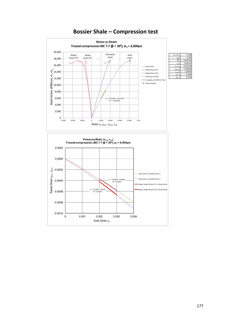
177
Bossier Shale – Compression test
13= 17,468
3= 6,000
E= 2.67E+06
a= 0.008164
ET1= -0.001306
ET2= -0.002828
vol= 0.00403
vzx = 0.2064
vzy = 0.2392
y = 2.67E+06x + 4.87E+02R² = 1.00E+00
0
2,000
4,000
6,000
8,000
10,000
12,000
14,000
16,000
18,000
20,000
-0.006 -0.004 -0.002 0 0.002 0.004 0.006 0.008 0.01
Axi
al s
tres
s d
iffe
nce
, 1-
3
Strain εa, εET1, εET2, εvol
Stress vs Strain
Triaxial compression JBC 7-7 ( = 300), 3 = 6,000psi
Axial Strain
Radial Strain ET1
Radial Strain ET2
Volumetric Strain
E modulus 33-49% of Yield
Peak strength
Radial strain ET2
Radial
strain ET1
y = -0.2064x + 0.0000R² = 0.9995
y = -0.2392x + 6E-05R² = 0.9994
-0.0010
-0.0008
-0.0006
-0.0004
-0.0002
0.0000
0.0002
0 0.001 0.002 0.003 0.004
Rad
ial S
train
εE
T1, ε E
T2
Axial Strain εa
Axial strain vs Radial Strain 1
Axial strain vs Radial Strain 2
Slope: Radial Strain ET1 vs Axial Strain
Slope: Radial Strain ET2 vs Axial Strain
Poissons Ratio, (n zy, n zx)
Triaxial compression JBC 7-7 ( = 300), 3 = 6,000psi
Volumetric
strainAxial
strain

178
Bossier Shale – Compression test
13= 18,026
3= 6,000
E= 2.74E+06
a= 0.00733
ET1= -0.001886
ET2= -0.003266
vol= 0.002178
vzx = 0.2190
vzy = 0.2608
y = 2.74E+06x + 7.00E+02R² = 1.00E+00
0
2000
4000
6000
8000
10000
12000
14000
16000
18000
20000
-0.004 -0.002 0 0.002 0.004 0.006 0.008
Axi
al s
tres
s d
iffe
nce
, 1-
3
Strain εa, εET1, εET2, εvol
Stress vs Strain
Triaxial compression JBC 7-8 ( = 300), 3 = 6,000psi
Axial Strain
Radial Strain ET1
Radial Strain ET2
Volumetric Strain
E modulus 33-49% of Yield
Peak strength
y = -0.2190x + 0.0000R² = 0.9995
y = -0.2608x + 2E-05R² = 0.9996
-0.0010
-0.0008
-0.0006
-0.0004
-0.0002
0.0000
0.0002
0 0.001 0.002 0.003 0.004
Rad
ial S
train
εE
T1, ε E
T2
Axial Strain εa
Axial strain vs Radial Strain 1
Axial strain vs Radial Strain 2
Slope: Radial Strain ET1 vs Axial Strain
Slope: Radial Strain ET2 vs Axial Strain
Poissons Ratio, (n zy, n zx)
Triaxial compression JBC 7-8 ( = 300), 3 = 6,000psi

179
Bossier Shale – Compression test
13= 16,722
3= 6,000
E= 2.62E+06
a= 0.007064
ET1= -0.001607
ET2= -0.001788
vol= 0.003669
vzx = 0.2169
vzy = 0.2264
y = 2.62E+06x + 5.27E+02R² = 1.00E+00
0
2000
4000
6000
8000
10000
12000
14000
16000
18000
20000
-0.004 -0.002 0 0.002 0.004 0.006 0.008
Axi
al s
tres
s d
iffe
nce
, 1-
3
Strain εa, εET1, εET2, εvol
Stress vs Strain
Triaxial compression JBC 7-3 ( = 450), 3 = 6,000psi
Axial Strain
Radial Strain ET1
Radial Strain ET2
Volumetric Strain
E modulus 24-50% of Yield
Peak strength
y = -0.2169x + 0.0001R² = 0.9997
y = -0.2264x + 6E-05R² = 0.9996
-0.0010
-0.0008
-0.0006
-0.0004
-0.0002
0.0000
0 0.001 0.002 0.003 0.004
Rad
ial S
train
εE
T1, ε E
T2
Axial Strain εa
Axial strain vs Radial Strain 1
Axial strain vs Radial Strain 2
Slope: Radial Strain ET1 vs Axial Strain
Slope: Radial Strain ET2 vs Axial Strain
Poissons Ratio, (n zy, n zx)
Triaxial compression JBC 7-3 ( = 450), 3 = 6,000psi

180
Bossier Shale – Compression test
13= 14,330
3= 6,000
E= 3.78E+06
a= 0.004151
ET1= -0.000944
ET2= -0.001443
vol= 0.001764
vzx = 0.1938
vzy = 0.2502
y = 3.78E+06x + 5.63E+02R² = 9.99E-01
0
2000
4000
6000
8000
10000
12000
14000
16000
-0.003 -0.002 -0.001 0 0.001 0.002 0.003 0.004 0.005
Axi
al s
tres
s d
iffe
nce
, 1-
3
Strain εa, εET1, εET2, εvol
Stress vs StrainTriaxial compression JBC 7-4 ( = 600), 3 = 6,000psi
Axial Strain
Radial Strain ET1
Radial Strain ET2
Volumetric Strain
E modulus 24-50% of Yield
Peak strength
y = -0.1938x + 0.0001R² = 0.9987
y = -0.2502x - 0.0001R² = 0.9992
-0.0010
-0.0008
-0.0006
-0.0004
-0.0002
0.0000
0 0.001 0.002 0.003
Rad
ial S
train
εE
T1, ε E
T2
Axial Strain εa
Axial strain vs Radial Strain 1
Axial strain vs Radial Strain 2
Slope: Radial Strain ET1 vs Axial Strain
Slope: Radial Strain ET2 vs Axial Strain
Poissons Ratio, (n zy, n zx)
Triaxial compression JBC 7-4 ( = 600), 3 = 6,000psi

181
Bossier Shale – Compression test
13= 31,437
3= 6,000
E= 7.54E+06
a= 0.00504
ET1= -0.000657
ET2= -0.002314
vol= 0.002069
vzx = 0.2604
vzy = 0.2114
y = 7.54E+06x - 3.15E+02R² = 1.00E+00
0
5000
10000
15000
20000
25000
30000
35000
-0.003 -0.002 -0.001 0 0.001 0.002 0.003 0.004 0.005 0.006
Axi
al s
tres
s d
iffe
nce
, 1-
3
Strain εa, εET1, εET2, εvol
Stress vs Strain
Triaxial compression JBC 7-1 ( = 900), 3 = 6,000psi
Axial Strain
Radial Strain ET1
Radial Strain ET2
Volumetric Strain
E modulus 26-50% of Yield
Peak strength
y = -0.2114x + 0.0000R² = 0.9998
y = -0.2604x + 5E-05R² = 0.9997
-0.0010
-0.0008
-0.0006
-0.0004
-0.0002
0.0000
0 0.001 0.002 0.003 0.004
Rad
ial S
train
εE
T1, ε E
T2
Axial Strain εa
Axial strain vs Radial Strain 1
Axial strain vs Radial Strain 2
Slope: Radial Strain ET1 vs Axial Strain
Slope: Radial Strain ET2 vs Axial Strain
Poissons Ratio, (n zy, n zx)
Triaxial compression JBC 7-1 ( = 900), 3 = 6,000psi

182
Bossier Shale – Compression test
1-3= 32,614
3= 10,000
E= 2.61E+06
a= 0.014577
ET1= -0.003235
ET2= -0.004098
vol= 0.007244
vzx = 0.1456
vzy = 0.2024
y = 2.61E+06x + 1.24E+03R² = 1.00E+00
0
5000
10000
15000
20000
25000
30000
35000
-0.01 -0.005 0 0.005 0.01 0.015 0.02
Axia
l str
ess,
Strain εa, εET1, εET2, εvol
Stress vs Strain
Triaxial compression JBC 5-5 ( = 00), 3 = 10,000psi
Axial Strain
Radial Strain ET1
Radial Strain ET2
Volumetric Strain
E modulus 20-28% of Yield
Peak strength
y = -0.1456x - 0.0000R² = 0.9996
y = -0.2024x - 3E-05R² = 0.9996
-0.0010
-0.0008
-0.0006
-0.0004
-0.0002
0.0000
0.0002
0 0.001 0.002 0.003 0.004
Rad
ial S
train
εE
T1, ε E
T2
Axial Strain εa
Axial strain vs Radial Strain 1
Axial strain vs Radial Strain 2
Slope: Radial Strain ET1 vs Axial Strain
Slope: Radial Strain ET2 vs Axial Strain
Poissons Ratio, (n zy, n zx)
Triaxial compression JBC 5-5 ( = 00), 3 = 10,000psi

183
Bossier Shale – Compression test
1-3= 28,263
3= 10,000
E= 4.21E+06
a= 0.007673
ET1= -0.001908
ET2= -0.001719
vol= 0.004046
vzx = 0.2388
vzy = 0.2164
y = 4.21E+06x + 4.74E+02R² = 1.00E+00
0
5000
10000
15000
20000
25000
30000
-0.004 -0.002 0 0.002 0.004 0.006 0.008 0.01
Axia
l str
ess,
Strain εa, εET1, εET2, εvol
Stress vs StrainTriaxial compression JBC 5-8 ( = 100), 3 = 10,000psi
Axial Strain
Radial Strain ET1
Radial Strain ET2
Volumetric Strain
E modulus 31-46% of Yield
Peak strength
y = -0.2388x + 0.0000R² = 0.9997
y = -0.2164x + 3E-05R² = 0.9996
-0.0010
-0.0008
-0.0006
-0.0004
-0.0002
0.0000
0.0002
0 0.001 0.002 0.003 0.004
Rad
ial S
train
εE
T1, ε E
T2
Axial Strain εa
Axial strain vs Radial Strain 1
Axial strain vs Radial Strain 2
Slope: Radial Strain ET1 vs Axial Strain
Slope: Radial Strain ET2 vs Axial Strain
Poissons Ratio, (n zy, n zx)
Triaxial compression JBC 5-8 ( = 100), 3 = 10,000psi

184
Bossier Shale – Compression test
1-3= 32,278
3= 10,000
E= 4.26E+06
a= 0.01024
ET1= -0.002801
ET2= -0.002447
vol= 0.004992
vzx = 0.2333
vzy = 0.2157
y = 4.26E+06x + 4.38E+01R² = 1.00E+00
0
5000
10000
15000
20000
25000
30000
35000
-0.006 -0.004 -0.002 0 0.002 0.004 0.006 0.008 0.01 0.012
Axia
l str
ess,
Strain εa, εET1, εET2, εvol
Stress vs StrainTriaxial compression JBC 5-9 ( = 150), 3 = 10,000psi
Axial Strain
Radial Strain ET1
Radial Strain ET2
Volumetric Strain
E modulus 26-40% of Yield
Peak strength
y = -0.2333x + 0.0001R² = 0.9998
y = -0.2157x + 4E-05R² = 0.9997
-0.0010
-0.0008
-0.0006
-0.0004
-0.0002
0.0000
0 0.001 0.002 0.003 0.004
Rad
ial S
train
εE
T1, ε E
T2
Axial Strain εa
Axial strain vs Radial Strain 1
Axial strain vs Radial Strain 2
Slope: Radial Strain ET1 vs Axial Strain
Slope: Radial Strain ET2 vs Axial Strain
Poissons Ratio, (n zy, n zx)
Triaxial compression JBC 5-9 ( = 150), 3 = 10,000psi

185
Bossier Shale – Compression test
1-3= 26,198
3= 10,000
E= 2.70E+06
a= 0.012005
ET1= -0.003732
ET2= -0.003479
vol= 0.004794
vzx = 0.2127
vzy = 0.2448
y = 2.70E+06x - 6.97E+02R² = 9.99E-01
0
5000
10000
15000
20000
25000
30000
-0.01 -0.005 0 0.005 0.01 0.015
Axia
l str
ess,
Strain εa, εET1, εET2, εvol
Stress vs Strain
Triaxial compression JBC 5-2 ( = 300), 3 = 10,000psi
Axial Strain
Radial Strain ET1
Radial Strain ET2
Volumetric Strain
E modulus 18-28% of Yield
Peak strength
y = -0.2127x + 0.0001R² = 0.9993
y = -0.2448x + 8E-05R² = 0.9993
-0.0010
-0.0008
-0.0006
-0.0004
-0.0002
0.0000
0 0.001 0.002 0.003 0.004
Rad
ial S
train
εE
T1, ε E
T2
Axial Strain εa
Axial strain vs Radial Strain 1
Axial strain vs Radial Strain 2
Slope: Radial Strain ET1 vs Axial Strain
Slope: Radial Strain ET2 vs Axial Strain
Poissons Ratio, (n zy, n zx)
Triaxial compression JBC 5-2 ( = 300), 3 = 10,000psi

186
Bossier Shale – Compression test
1-3= 22,556
3= 10,000
E= 2.94E+06
a= 0.00931
ET1= -0.003458
ET2= -0.00294
vol= 0.002912
vzx = 0.2792
vzy = 0.2964
y = 2.94E+06x + 9.70E+01R² = 1.00E+00
0
5000
10000
15000
20000
25000
-0.006 -0.004 -0.002 0 0.002 0.004 0.006 0.008 0.01 0.012
Axia
l str
ess,
Strain εa, εET1, εET2, εvol
Stress vs Strain
Triaxial compression JBC 5-3 ( = 450), 3 = 10,000psi
Axial Strain
Radial Strain ET1
Radial Strain ET2
Volumetric Strain
E modulus 26-40% of Yield
Peak strength
y = -0.2792x + 0.0002R² = 0.9992
y = -0.2964x - 1E-06R² = 0.9997
-0.0010
-0.0008
-0.0006
-0.0004
-0.0002
0.0000
0.0002
0 0.001 0.002 0.003 0.004
Rad
ial S
train
εE
T1, ε E
T2
Axial Strain εa
Axial strain vs Radial Strain 1
Axial strain vs Radial Strain 2
Slope: Radial Strain ET1 vs Axial Strain
Slope: Radial Strain ET2 vs Axial Strain
Poissons Ratio, (n zy, n zx)
Triaxial compression JBC 5-3 ( = 450), 3 = 10,000psi

187
Bossier Shale – Compression test
1-3= 23,197
3= 10,000
E= 4.15E+06
a= 0.007123
ET1= -0.002771
ET2= -0.002826
vol= 0.001526
vzx = 0.2611
vzy = 0.3067
y = 4.15E+06x + 9.38E+02R² = 1.00E+00
0
5000
10000
15000
20000
25000
-0.006 -0.004 -0.002 0 0.002 0.004 0.006 0.008 0.01
Axia
l str
ess,
Strain εa, εET1, εET2, εvol
Stress vs Strain
Triaxial compression JBC 5-4 ( = 600), 3 = 10,000psi
Axial Strain
Radial Strain ET1
Radial Strain ET2
Volumetric Strain
E modulus 33-50% of Yield
Peak strength
y = -0.2611x + 0.0001R² = 0.9994
y = -0.3067x - 5E-06R² = 0.9997
-0.0010
-0.0008
-0.0006
-0.0004
-0.0002
0.0000
0 0.001 0.002 0.003 0.004
Rad
ial S
train
εE
T1, ε E
T2
Axial Strain εa
Axial strain vs Radial Strain 1
Axial strain vs Radial Strain 2
Slope: Radial Strain ET1 vs Axial Strain
Slope: Radial Strain ET2 vs Axial Strain
Poissons Ratio, (n zy, n zx)
Triaxial compression JBC 5-4 ( = 600), 3 = 10,000psi

188
Bossier Shale – Compression test
1-3= 29,812
3= 10,000
E= 7.51E+06
a= 0.005216
ET1= -0.001655
ET2= -0.002187
vol= 0.001374
vzx = 0.2664
vzy = 0.3659
y = 7.51E+06x + 2.14E+02R² = 9.99E-01
0
5000
10000
15000
20000
25000
30000
35000
-0.004 -0.003 -0.002 -0.001 0 0.001 0.002 0.003 0.004 0.005 0.006
Axia
l str
ess,
Strain εa, εET1, εET2, εvol
Stress vs Strain
Triaxial compression JBC 5-6 ( = 750), 3 = 10,000psi
Axial Strain
Radial Strain ET1
Radial Strain ET2
Volumetric Strain
E modulus 20-45% of Yield
Peak strength
y = -0.2664x + 0.0000R² = 0.9993
y = -0.3659x + 4E-05R² = 0.9994
-0.0010
-0.0008
-0.0006
-0.0004
-0.0002
0.0000
0.0002
0 0.001 0.002 0.003 0.004
Rad
ial S
train
εE
T1, ε E
T2
Axial Strain εa
Axial strain vs Radial Strain 1
Axial strain vs Radial Strain 2
Slope: Radial Strain ET1 vs Axial Strain
Series5
Poissons Ratio, (n zy, n zx)
Triaxial compression JBC 5-6 ( = 750), 3 = 10,000psi

189
Bossier Shale – Compression test
1-3= 37,097
3= 10,000
E= 8.19E+06
a= 0.004846
ET1= -0.001513
ET2= -0.001999
vol= 0.001334
vzx = 0.3594
vzy = 0.3038
y = 8.19E+06x + 2.41E+03R² = 9.99E-01
0
5000
10000
15000
20000
25000
30000
35000
40000
-0.003 -0.002 -0.001 0 0.001 0.002 0.003 0.004 0.005 0.006
Axia
l str
ess,
Strain εa, εET1, εET2, εvol
Stress vs Strain
Triaxial compression JBC 5-1 ( = 900), 3 = 10,000psi
Axial Strain
Radial Strain ET1
Radial Strain ET2
Volumetric Strain
E modulus 20-28% of Yield
Peak strength
y = -0.3038x - 0.0000R² = 0.9990
y = -0.3594x - 8E-05R² = 0.999
-0.0010
-0.0008
-0.0006
-0.0004
-0.0002
0.0000
0 0.001 0.002 0.003 0.004
Rad
ial S
train
εE
T1, ε E
T2
Axial Strain εa
Axial strain vs Radial Strain 1
Axial strain vs Radial Strain 2
Slope: Radial Strain ET1 vs Axial Strain
Slope: Radial Strain ET2 vs Axial Strain
Poissons Ratio, (n zy, n zx)
Triaxial compression JBC 5-1 ( = 900), 3 = 10,000psi

190
Bossier Shale – Extension test
13= 7,796
3= 228
E= 3.67E+06
a= -0.00325114
ET1= -0.00018799
ET2= 0.002717798
vol= -0.00072133
vzx = 0.1057
vzy = 0.2820
y = -3.67E+06x + 5.42E+02R² = 9.97E-01
0.0
1000.0
2000.0
3000.0
4000.0
5000.0
6000.0
7000.0
8000.0
9000.0
-0.0080 -0.0060 -0.0040 -0.0020 0.0000 0.0020 0.0040 0.0060 0.0080 0.0100 0.0120
Axia
l str
ess d
iff,
-(
1
3
Strain εa, εET1, εET2, εvol
Stress vs StrainTriaxial extension JBC 9-1 ( = 450), 1 = 8,024psi
Axial Strain
Radial Strain ET1
Radial Strain ET2
Volumetric Strain
Peak strength
E modulus
y = -0.1057x - 0.0000R² = 0.8797
y = -0.282x - 4E-06R² = 0.9803
-0.0001
0.0000
0.0001
0.0002
0.0003
0.0004
0.0005
0.0006
0.0007
-0.0025 -0.0020 -0.0015 -0.0010 -0.0005 0.0000
Rad
ial S
train
εE
T1, ε E
T2
Axial Strain εa
Axial strain vs Radial Strain 1
Axial strain vs Radial Strain 2
Slope: Radial Strain ET1 vs Axial Strain
Slope: Radial Strain ET2 vs Axial Strain
Poissons Ratio, (n zy, n zx)
Triaxial compression MUE 9-1 ( = 450), 1 = 8,024psi

191
Bossier Shale – Extension test
13= 10,709
3= 2,610
E= 3.95E+06
a= -0.00342954
ET1= -0.00016641
ET2= 0.000776718
vol= -0.00281923
vzx = 0.1198
vzy = 0.1808
y = -3.95E+06x + 5.56E+01R² = 9.95E-01
0.0
2000.0
4000.0
6000.0
8000.0
10000.0
12000.0
-0.0070 -0.0060 -0.0050 -0.0040 -0.0030 -0.0020 -0.0010 0.0000 0.0010 0.0020
Axia
l str
ess d
iff,
-(
1
3
Strain εa, εET1, εET2, εvol
Stress vs StrainTriaxial extension JBC 3-1 ( = 600), 1 = 13,334psi
Axial Strain
Radial Strain ET1
Radial Strain ET2
Volumetric Strain
E modulus
Peak strength
y = 0.1198x + 0.0000R² = 0.8046
y = -0.1808x - 0.0001R² = 0.8759
-0.0004
-0.0002
0.0000
0.0002
0.0004
0.0006
0.0008
0.0010
-0.0020 -0.0015 -0.0010 -0.0005 0.0000
Rad
ial S
train
εE
T1, ε E
T2
Axial Strain εa
Axial strain vs Radial Strain 1
Axial strain vs Radial Strain 2
Slope: Radial Strain ET1 vs Axial Strain
Slope: Radial Strain ET2 vs Axial Strain
Poissons Ratio, (n zy, n zx)
Triaxial compression MUE 3-1 ( = 600), 1 = 13,334psi

192
Bossier Shale – Extension test
13= 17,923
3= 7,085
E= 5.62E+06
a= -0.00420461
ET1= 0.000767473
ET2= 0.002395817
vol= -0.00104132
vzx = 0.2409
vzy = 0.4097
y = -5.62E+06x + 3.08E+02R² = 9.98E-01
0
2000
4000
6000
8000
10000
12000
14000
16000
18000
20000
-0.0080 -0.0060 -0.0040 -0.0020 0.0000 0.0020 0.0040
Axia
l str
ess d
iff,
-(
1
3
Strain εa, εET1, εET2, εvol
Stress vs StrainTriaxial extension JBC 6-3 ( = 300), 1 = 25,007psi
Axial Strain
Radial Strain ET1
Radial Strain ET2
Volumetric Strain
E modulus
Peak strength
y = -0.2409x - 0.0000R² = 0.9591
y = -0.4097x - 5E-05R² = 0.972
-0.0005
0.0000
0.0005
0.0010
0.0015
0.0020
-0.0020 -0.0015 -0.0010 -0.0005 0.0000
Rad
ial S
train
εE
T1, ε E
T2
Axial Strain εa
Axial strain vs Radial Strain 1
Axial strain vs Radial Strain 2
Slope: Radial Strain ET1 vs Axial Strain
Slope: Radial Strain ET2 vs Axial Strain
Poissons Ratio, (n zy, n zx)
Triaxial compression MUE 6-3 ( = 300), 1 = 25,007psi

193
Bossier Shale – Extension test
13= 17,331
3= 7,661
E= 5.19E+06
a= -0.00513524
ET1= 0.000597042
ET2= 0.003024213
vol= -0.00151398
vzx = 0.125
vzy = 0.3866
y = -5.19E+06x + 2.75E+01R² = 9.78E-01
0.0
2000.0
4000.0
6000.0
8000.0
10000.0
12000.0
14000.0
16000.0
18000.0
20000.0
-0.0100 -0.0080 -0.0060 -0.0040 -0.0020 0.0000 0.0020 0.0040
Axia
l str
ess d
iff,
-(
1
3
Strain εa, εET1, εET2, εvol
Stress vs Strain
Triaxial extension JBC 6-5 ( = 450), 1 = 24,993psi
Axial Strain
Radial Strain ET1
Radial Strain ET2
Volumetric Strain
E modulus
Peak strength
y = -0.1250x - 0.0000R² = 0.5396
y = -0.3866x - 1E-05R² = 0.9126
-0.0005
0.0000
0.0005
0.0010
0.0015
0.0020
-0.0020 -0.0015 -0.0010 -0.0005 0.0000
Rad
ial S
train
εE
T1, ε E
T2
Axial Strain εa
Axial strain vs Radial Strain 1
Axial strain vs Radial Strain 2
Slope: Radial Strain ET1 vs Axial Strain
Slope: Radial Strain ET2 vs Axial Strain
Poissons Ratio, (n zy, n zx)
Triaxial compression MUE 6-5 ( = 450), 1 = 24,993psi

194
Bossier Shale – Extension test
13= 17,817
3= 7,190
E= 4.48E+06
a= -0.00511752
ET1= 0.000840627
ET2= 0.002503805
vol= -0.00177309
vzx = 0.1597
vzy = 0.4056
y = -4.48E+06x + 7.43E+02R² = 9.97E-01
0.0
2000.0
4000.0
6000.0
8000.0
10000.0
12000.0
14000.0
16000.0
18000.0
20000.0
-0.0100 -0.0080 -0.0060 -0.0040 -0.0020 0.0000 0.0020 0.0040
Axia
l str
ess d
iff,
-(
1
3
Strain εa, εET1, εET2, εvol
Stress vs StrainTriaxial extension JBC 6-4 ( = 600), 1 = 25,007psi
Axial Strain
Radial Strain ET1
Radial Strain ET2
Volumetric Strain
E modulus
Peak strength
y = -0.1597x + 0.0000R² = 0.9426
y = -0.4056x + 4E-05R² = 0.9869
-0.0005
0.0000
0.0005
0.0010
0.0015
0.0020
-0.0020 -0.0015 -0.0010 -0.0005 0.0000
Rad
ial S
train
εE
T1, ε E
T2
Axial Strain εa
Axial strain vs Radial Strain 1
Axial strain vs Radial Strain 2
Slope: Radial Strain ET1 vs Axial Strain
Slope: Radial Strain ET2 vs Axial Strain
Poissons Ratio, (n zy, n zx)
Triaxial compression MUE 6-4 ( = 600), 1 = 25,007psi

195
A2 Vaca Muerta shale experimental data
Vaca Muerta Shale – Summary of experimental results
Sample
ID
Bulk
Density 13 3 Ez a ET1 ET2 vol vzx vzy
angle (g/cm3) (psi) (psi) (psi)
Compression test MUE 1-1 0 2.465 13,730 0 2.670E+06 0.006367 -0.000961 -0.001001 0.004405 0.1586 0.1690
Compression test MUE 1-11 60 2.456 7,874 0 3.030E+06 0.0029 -0.003215 -0.000991 -0.001306 0.2207 0.0965
Compression test MUE 1-4 0 2.47 19,118 1,000 2.650E+06 0.008679 -0.001971 -0.001995 0.004713 0.185 0.1877
Compression test MUE 1-9 60 2.434 11,337 1,000 3.770E+06 0.003259 -0.000857 -0.001049 0.001353 0.2568 0.2864
Compression test MUE 1-16 90 2.432 18,073 1,000 3.800E+06 0.00536 -0.005983 -0.000887 -0.00151 0.4195 0.2793
Compression test MUE1-33 15 2.393 17,604 2,500 1.680E+06 0.014801 -0.004027 -0.003228 0.007546 0.2164 0.1346
Compression test MUE 1-22 20 2.46 19,451 2,500 2.300E+06 0.012081 -0.006045 -0.005598 0.000438 0.2617 0.2186
Compression test MUE1-32 30 2.429 18,036 2,500 2.190E+06 0.011023 -0.003189 -0.003514 0.00432 0.2104 0.1996
Compression test MUE1-27 40 2.421 15,507 2,500 2.200E+06 0.009666 -0.003237 -0.002728 0.003701 0.2324 0.1664
Compression test MUE 1-8 50 2.427 14,512 2,500 2.660E+06 0.007998 -0.003035 -0.001751 0.003212 0.2781 0.1666
Compression test MUE1-28 75 2.377 17,433 2,500 3.000E+06 0.008272 -0.002348 -0.003285 0.002639 0.2015 0.3286
Compression test MUE 1-18 90 2.395 19,347 2,500 3.760E+06 0.005929 -0.001725 -0.001769 0.002435 0.2485 0.2599
Compression test MUE 1-2 0 2.464 25,744 5,000 2.120E+06 0.017101 -0.004515 -0.004311 0.008275 0.1998 0.1900
Compression test MUE 1-5 10 2.465 25,629 5,000 2.150E+06 0.017546 -0.004824 -0.003895 0.008827 0.1895 0.1761
Compression test MUE 1-21 40 2.447 24,355 5,000 3.010E+06 0.012017 -0.004343 -0.004881 0.002793 0.2137 0.2071
Compression test MUE 1-10 60 2.451 18,913 5,000 4.100E+06 0.005754 -0.00171 -0.000904 0.00314 0.2408 0.2006
Compression test MUE 1-14 80 2.477 28,639 5,000 4.660E+06 0.007758 -0.002374 -0.00199 0.003394 0.2551 0.2282
Compression test MUE 1-19 90 2.393 22,673 5,000 3.520E+06 0.008917 -0.00215 -0.002433 0.004334 0.2249 0.2256
Compression test MUE 1-3 0 2.464 49,963 20,000 2.350E+06 0.067036 -0.022181 -0.022008 0.022847 0.1605 0.1474
Compression test MUE 1-12 60 2.43 41,119 20,000 3.010E+06 0.058103 -0.021896 -0.037697 -0.00149 0.1909 0.1849
Compression test MUE1-20 90 2.427 47,894 20,000 4.440E+06 0.081562 -0.059534 -0.042261 -0.020233 0.2499 0.203
Extension test MUE 1-24 0 2.454 23,802 1,161 4.740E+06 -0.007755222 0.003801683 0.001848205 -0.002105334 0.2666 0.4501
Extension test MUE 1-25 60 2.458 19,510 3,109 3.250E+06 -0.00820747 0.002294112 0.004119127 -0.001794231 0.2289 0.4239
Ev = 2.45E+06
Eh = 3.88E+06
vv= 0.1748
vh= 0.2420
Gsv= 1.24E+06
Triaxial
experiment
type
Average E moduli
strain in (in/in) at failure

196
Vaca Muerta Shale – Compression test
13= 13,730
3= 0
E= 2.67E+06
a= 0.006367
ET1= -0.000961
ET2= -0.001001
vol= 0.004405
vzx = 0.1586
vzy = 0.1690
y = 2.67E+06x - 1.30E+03R² = 1.00E+00
0
2000
4000
6000
8000
10000
12000
14000
16000
-0.008 -0.006 -0.004 -0.002 0 0.002 0.004 0.006 0.008 0.01
Axia
l str
ess d
iff,
(1
3
Strain εa, εET1, εET2, εvol
Stress vs StrainTriaxial compression MUE 1-1 ( = 00), 3 = UCS
Axial Strain
Radial Strain ET1
Radial Strain ET2
Volumetric Strain
E modulus 40-50% of Yield
Peak strength
y = -0.1586x + 0.0001R² = 0.9993
y = -0.169x + 0.0002R² = 0.9992
-0.0010
-0.0008
-0.0006
-0.0004
-0.0002
0.0000
0.0002
0 0.001 0.002 0.003 0.004
Rad
ial S
train
εE
T1, ε E
T2
Axial Strain εa
Axial strain vs Radial Strain 1
Axial strain vs Radial Strain 2
Slope: Radial Strain ET1 vs Axial Strain
Slope: Radial Strain ET2 vs Axial Strain
Poissons Ratio, (n zy, n zx)
Triaxial compression MUE 1-1 ( = 00), 3 = UCS

197
Vaca Muerta Shale – Compression test
13= 7,874
3= 0
E= 3.03E+06
a= 0.0029
ET1= -0.003215
ET2= -0.000991
vol= -0.001306
vzx = 0.2207
vzy = 0.0965
y = 3.03E+06x - 3.03E+02R² = 1.00E+00
0
1000
2000
3000
4000
5000
6000
7000
8000
9000
-0.004 -0.003 -0.002 -0.001 0 0.001 0.002 0.003 0.004
Axia
l str
ess d
iff,
(1
3
Strain εa, εET1, εET2, εvol
Stress vs StrainTriaxial compression MUE 1-11 ( = 600), 3 = UCS
Axial Strain
Radial Strain ET1
Radial Strain ET2
Volumetric Strain
E modulus 40-50% of Yield
Peak strength
y = -0.2207x + 0.0001R² = 0.9836
y = -0.0965x - 9E-06R² = 0.9685
-0.0010
-0.0008
-0.0006
-0.0004
-0.0002
0.0000
0 0.001 0.002 0.003 0.004
Rad
ial S
train
εE
T1, ε E
T2
Axial Strain εa
Axial strain vs Radial Strain 1
Axial strain vs Radial Strain 2
Slope: Radial Strain ET1 vs Axial Strain
Slope: Radial Strain ET2 vs Axial Strain
Poissons Ratio, (n zy, n zx)
Triaxial compression MUE 1-11 ( = 600), 3 = UCS

198
Vaca Muerta Shale – Compression test
13= 19,118
3= 1,000
E= 2.65E+06
a= 0.008679
ET1= -0.001971
ET2= -0.001995
vol= 0.004713
vzx = 0.1850
vzy = 0.1877
y = 2.65E+06x + 1.27E+03R² = 1.00E+00
0
5000
10000
15000
20000
25000
-0.01 -0.005 0 0.005 0.01 0.015
Axia
l str
ess d
iff,
(1
3
Strain εa, εET1, εET2, εvol
Stress vs StrainTriaxial compression MUE 1-4 ( = 00), 3 = 1,000psi
Axial Strain
Radial Strain ET1
Radial Strain ET2
Volumetric Strain
E modulus 40-50% of Yield
Peak strength
y = -0.1850x + 0.0000R² = 0.9992
y = -0.1877x + 5E-05R² = 0.9996
-0.0010
-0.0008
-0.0006
-0.0004
-0.0002
0.0000
0 0.001 0.002 0.003 0.004
Rad
ial S
train
εE
T1, ε E
T2
Axial Strain εa
Axial strain vs Radial Strain 1
Axial strain vs Radial Strain 2
Slope: Radial Strain ET1 vs Axial Strain
Slope: Radial Strain ET2 vs Axial Strain
Poissons Ratio, (n zy, n zx)
Triaxial compression MUE 1-4 ( = 00), 3 = 1,000psi

199
Vaca Muerta Shale – Compression test
13= 11,337
3= 1,000
E= 3.77E+06
a= 0.003259
ET1= -0.000857
ET2= -0.001049
vol= 0.001353
vzx = 0.2568
vzy = 0.2864
y = 3.77E+06x + 4.77E+02R² = 1.00E+00
0
2000
4000
6000
8000
10000
12000
-0.012 -0.008 -0.004 0 0.004 0.008 0.012
Axia
l str
ess d
iff,
(1
3
Strain εa, εET1, εET2, εvol
Stress vs StrainTriaxial compression MUE 1-9 ( = 600), 3 = 1,000psi
Axial Strain
Radial Strain ET1
Radial Strain ET2
Volumetric Strain
E modulus 40-50% of Yield
Peak strength
y = -0.2568x + 0.0000R² = 0.9983
y = -0.2864x + 3E-05R² = 0.9979
-0.0010
-0.0008
-0.0006
-0.0004
-0.0002
0.0000
0.0002
0 0.001 0.002 0.003
Rad
ial S
train
εE
T1, ε E
T2
Axial Strain εa
Axial strain vs Radial Strain 1
Axial strain vs Radial Strain 2
Slope: Radial Strain ET1 vs Axial Strain
Slope: Radial Strain ET2 vs Axial Strain
Poissons Ratio, (n zy, n zx)
Triaxial compression MUE 1-9 ( = 600), 3 = 1,000psi

200
Vaca Muerta Shale – Compression test
13= 18,073
3= 1,000
E= 3.80E+06
a= 0.00536
ET1= -0.005983
ET2= -0.000887
vol= -0.00151
vzx = 0.2793
vzy = 0.4195
y = 3.80E+06x + 2.25E+03R² = 1.00E+00
0
2000
4000
6000
8000
10000
12000
14000
16000
18000
20000
-0.01 -0.006 -0.002 0.002 0.006 0.01
Axia
l str
ess d
iff,
(1
3
Strain εa, εET1, εET2, εvol
Stress vs StrainTriaxial compression MUE 1-16 ( = 900), 3 = 1,000psi
Axial Strain
Radial Strain ET1
Radial Strain ET2
Volumetric Strain
E modulus 40-50% of Yield
Peak strength
y = -0.4195x + 0.0002R² = 0.9996
y = -0.2793x + 7E-05R² = 0.9989
-0.0015
-0.0013
-0.0011
-0.0009
-0.0007
-0.0005
-0.0003
-0.0001
0 0.001 0.002 0.003 0.004
Rad
ial S
train
εE
T1, ε E
T2
Axial Strain εa
Axial strain vs Radial Strain 1
Axial strain vs Radial Strain 2
Slope: Radial Strain ET1 vs Axial Strain
Slope: Radial Strain ET2 vs Axial Strain
Poissons Ratio, (n zy, n zx)
Triaxial compression MUE 1-16 ( = 900), 3 = 1,000psi

201
Vaca Muerta Shale – Compression test
13= 17,604
3= 2,500
E= 1.68E+06
a= 0.014801
ET1= -0.004027
ET2= -0.003228
vol= 0.007546
vzx = 0.2164
vzy = 0.1346
y = 1.68E+06x + 1.50E+03R² = 1.00E+00
0
2000
4000
6000
8000
10000
12000
14000
16000
18000
20000
-0.01 -0.005 0 0.005 0.01 0.015 0.02
Axia
l str
ess d
iff,
(1
3
Strain εa, εET1, εET2, εvol
Stress vs StrainTriaxial compression MUE 1-33 ( = 150), 3 = 2,500psi
Axial Strain
Radial Strain ET1
Radial Strain ET2
Volumetric Strain
E modulus 40-50% of Yield
Peak strength
y = -0.2164x + 0.0001R² = 0.9999
y = -0.1346x - 3E-05R² = 0.9998
-0.0010
-0.0008
-0.0006
-0.0004
-0.0002
0.0000
0 0.002 0.004 0.006
Rad
ial S
train
εE
T1, ε E
T2
Axial Strain εa
Axial strain vs Radial Strain 1
Axial strain vs Radial Strain 2
Slope: Radial Strain ET1 vs Axial Strain
Slope: Radial Strain ET2 vs Axial Strain
Poissons Ratio, (n zy, n zx)
Triaxial compression MUE 1-33 ( = 150), 3 = 2,500psi

202
Vaca Muerta Shale – Compression test
13= 19,451
3= 2,500
E= 2.30E+06
a= 0.012081
ET1= -0.006045
ET2= -0.005598
vol= 0.000438
vzx = 0.2617
vzy = 0.2186
y = 2.30E+06x + 1.81E+03R² = 1.00E+00
0
5000
10000
15000
20000
25000
-0.01 -0.005 0 0.005 0.01 0.015
Axia
l str
ess d
iff,
(1
3
Strain εa, εET1, εET2, εvol
Stress vs StrainTriaxial compression MUE 1-22 ( = 200), 3 = 2,500psi
Axial Strain
Radial Strain ET1
Radial Strain ET2
Volumetric Strain
E modulus 40-50% of Yield
Peak strength
y = -0.2617x + 0.0002R² = 0.9994
y = -0.2186x + 9E-05R² = 0.9994
-0.0010
-0.0008
-0.0006
-0.0004
-0.0002
0.0000
0 0.001 0.002 0.003 0.004 0.005
Rad
ial S
train
εE
T1, ε E
T2
Axial Strain εa
Axial strain vs Radial Strain 1
Axial strain vs Radial Strain 2
Slope: Radial Strain ET1 vs Axial Strain
Slope: Radial Strain ET2 vs Axial Strain
Poissons Ratio, (n zy, n zx)
Triaxial compression MUE 1-22 ( = 200), 3 = 2,500psi

203
Vaca Muerta Shale – Compression test
13= 18,036
3= 2,500
E= 2.19E+06
a= 0.011023
ET1= -0.003189
ET2= -0.003514
vol= 0.00432
vzx = 0.2104
vzy = 0.1996
y = 2.19E+06x + 1.78E+03R² = 1.00E+00
0
2000
4000
6000
8000
10000
12000
14000
16000
18000
20000
-0.006 -0.004 -0.002 0 0.002 0.004 0.006 0.008 0.01 0.012
Axia
l str
ess d
iff,
(1
3
Strain εa, εET1, εET2, εvol
Stress vs StrainTriaxial compression MUE 1-32 ( = 300), 3 = 2,500psi
Axial Strain
Radial Strain ET1
Radial Strain ET2
Volumetric Strain
E modulus 40-50% of Yield
Peak Strength
y = -0.2104x + 0.0001R² = 0.9997
y = -0.1996x + 1E-05R² = 0.9998
-0.0010
-0.0008
-0.0006
-0.0004
-0.0002
0.0000
0 0.001 0.002 0.003 0.004 0.005
Rad
ial S
train
εE
T1, ε E
T2
Axial Strain εa
Axial strain vs Radial Strain 1
Axial strain vs Radial Strain 2
Slope: Radial Strain ET1 vs Axial Strain
Slope: Radial Strain ET2 vs Axial Strain
Poissons Ratio, (n zy, n zx)
Triaxial compression MUE 1-32 ( = 300), 3 = 2,500psi

204
Vaca Muerta Shale – Compression test
13= 15,507
3= 2,500
E= 2.20E+06
a= 0.009666
ET1= -0.003237
ET2= -0.002728
vol= 0.003701
vzx = 0.2324
vzy = 0.1664
y = 2.20E+06x + 1.53E+03R² = 1.00E+00
0
2000
4000
6000
8000
10000
12000
14000
16000
18000
-0.01 -0.005 0 0.005 0.01 0.015
Axia
l str
ess d
iff,
(1
3
Strain εa, εET1, εET2, εvol
Stress vs StrainTriaxial compression MUE 1-27 ( = 400), 3 = 2,500psi
Axial Strain
Radial Strain ET1
Radial Strain ET2
Volumetric Strain
E modulus 40-50% of Yield
Peak Strength
y = -0.2324x + 0.0002R² = 0.9997
y = -0.1664x + 2E-06R² = 0.9997
-0.0010
-0.0008
-0.0006
-0.0004
-0.0002
0.0000
0.0002
0 0.001 0.002 0.003 0.004 0.005
Rad
ial S
train
εE
T1, ε E
T2
Axial Strain εa
Axial strain vs Radial Strain 1
Axial strain vs Radial Strain 2
Slope: Radial Strain ET1 vs Axial Strain
Slope: Radial Strain ET2 vs Axial Strain
Poissons Ratio, (n zy, n zx)
Triaxial compression MUE 1-27 ( = 400), 3 = 2,500psi

205
Vaca Muerta Shale – Compression test
13= 14,512
3= 2,500
E= 2.66E+06
a= 0.007998
ET1= -0.003035
ET2= -0.001751
vol= 0.003212
vzx = 0.2781
vzy = 0.1666
y = 2.66E+06x + 4.02E+02R² = 1.00E+00
0
2000
4000
6000
8000
10000
12000
14000
16000
-0.006 -0.004 -0.002 0 0.002 0.004 0.006 0.008 0.01
Axia
l str
ess d
iff,
(1
3
Strain εa, εET1, εET2, εvol
Stress vs StrainTriaxial compression MUE 1-8 ( = 500), 3 = 2,500psi
Axial Strain
Radial Strain ET1
Radial Strain ET2
Volumetric Strain
E modulus 40-50% of Yield
Peak strength
y = -0.2781x - 0.0000R² = 0.9999
y = -0.1666x + 0.0001R² = 0.9985
-0.0010
-0.0008
-0.0006
-0.0004
-0.0002
0.0000
0.0002
0 0.001 0.002 0.003 0.004 0.005
Rad
ial S
train
εE
T1, ε E
T2
Axial Strain εa
Axial strain vs Radial Strain 1
Axial strain vs Radial Strain 2
Series4
Slope: Radial Strain ET2 vs Axial Strain
Poissons Ratio, (n zy, n zx)
Triaxial compression MUE 1-8 ( = 500), 3 = 2,500psi

206
Vaca Muerta Shale – Compression test
13= 17,433
3= 2,500
E= 3.00E+06
a= 0.008272
ET1= -0.002348
ET2= -0.003285
vol= 0.002639
vzx = 0.2015
vzy = 0.3286
y = 3.00E+06x + 1.61E+03R² = 1.00E+00
0
2000
4000
6000
8000
10000
12000
14000
16000
18000
20000
-0.006 -0.004 -0.002 0 0.002 0.004 0.006 0.008 0.01
Axia
l str
ess d
iff,
(1
3
Strain εa, εET1, εET2, εvol
Stress vs StrainTriaxial compression MUE 1-28 ( = 750), 3 = 2,500psi
Axial Strain
Radial Strain ET1
Radial Strain ET2
Volumetric Strain
E modulus 40-50% of Yield
Peak Strength
y = -0.2015x + 0.0000R² = 0.9996
y = -0.3286x + 5E-05R² = 0.9999
-0.0010
-0.0008
-0.0006
-0.0004
-0.0002
0.0000
0.0002
0 0.001 0.002 0.003 0.004 0.005
Rad
ial S
train
εE
T1, ε E
T2
Axial Strain εa
Axial strain vs Radial Strain 1
Axial strain vs Radial Strain 2
Slope: Radial Strain ET1 vs Axial Strain
Slope: Radial Strain ET2 vs Axial Strain
Poissons Ratio, (n zy, n zx)
Triaxial compression MUE 1-28 ( = 750), 3 = 2,500psi

207
Vaca Muerta Shale – Compression test
13= 19,347
3= 2,500
E= 3.76E+06
a= 0.005929
ET1= -0.001725
ET2= -0.001769
vol= 2.44E-03
vzx = 0.2599
vzy = 0.2485
y = 3.76E+06x + 1.79E+03R² = 1.00E+00
0
5,000
10,000
15,000
20,000
25,000
-0.006 -0.004 -0.002 0 0.002 0.004 0.006 0.008
Axia
l str
ess d
iff,
(1
3
Strain εa, εET1, εET2, εvol
Stress vs StrainTriaxial compression MUE 1-18 ( = 900), 3 = 2,500psi
Axial Strain
Radial Strain ET1
Radial Strain ET2
Volumetric Strain
E modulus 40-50% of Yield
Peak strength
y = -0.2485x - 0.0000R² = 0.9998
y = -0.2599x - 0.0000R² = 0.9998
-0.0010
-0.0008
-0.0006
-0.0004
-0.0002
0.0000
0 0.001 0.002 0.003 0.004 0.005
Rad
ial S
train
εE
T1, ε E
T2
Axial Strain εa
Axial strain vs Radial Strain 1
Axial strain vs Radial Strain 2
Slope: Radial Strain ET1 vs Axial Strain
Slope: Radial Strain ET2 vs Axial Strain
Poissons Ratio, (n zy, n zx)
Triaxial compression MUE 1-18 ( = 900), 3 = 2,500psi

208
Vaca Muerta Shale – Compression test
13= 25,744
3= 5,000
E= 2.12E+06
a= 0.017101
ET1= -0.004515
ET2= -0.004311
vol= 8.28E-03
vzx = 0.1998
vzy = 0.1900
y = 2.12E+06x + 2.24E+03R² = 1.00E+00
0
5,000
10,000
15,000
20,000
25,000
30,000
-0.01 -0.005 0 0.005 0.01 0.015 0.02 0.025
Axia
l str
ess d
iff,
(1
3
Strain εa, εET1, εET2, εvol
Stress vs StrainTriaxial compression MUE 1-2 ( = 00), 3 = 5,000psi
Axial Strain
Radial Strain ET1
Radial Strain ET2
Volumetric Strain
E modulus 40-50% of Yield
Peak strength
y = -0.1998x + 0.0001R² = 0.9993
y = -0.1900x + 0.0001R² = 0.9997
-0.0010
-0.0008
-0.0006
-0.0004
-0.0002
0.0000
0 0.002 0.004 0.006 0.008
Rad
ial S
train
εE
T1, ε E
T2
Axial Strain εa
Axial strain vs Radial Strain 1
Axial strain vs Radial Strain 2
Slope: Radial Strain ET1 vs Axial Strain
Slope: Radial Strain ET2 vs Axial Strain
Poissons Ratio, (n zy, n zx)
Triaxial compression MUE 1-2 ( = 00), 3 = 5,000psi

209
Vaca Muerta Shale – Compression test
13= 25,629
3= 5,000
E= 2.15E+06
a= 0.017546
ET1= -0.004824
ET2= -0.003895
vol= 8.83E-03
vzx = 0.1895
vzy = 0.1761
y = 2.15E+06x + 2.06E+03R² = 1.00E+00
0
5,000
10,000
15,000
20,000
25,000
30,000
-0.01 -0.005 0 0.005 0.01 0.015 0.02 0.025
Axia
l str
ess d
iff,
(1
3
Strain εa, εET1, εET2, εvol
Stress vs StrainTriaxial compression MUE 1-5 ( = 100), 3 = 5,000psi
Axial Strain
Radial Strain ET1
Radial Strain ET2
Volumetric Strain
E modulus 40-50% of Yield
Peak strength
y = -0.1895x + 0.0001R² = 0.9995
y = -0.1761x + 0.0000R² = 0.9995
-0.0010
-0.0008
-0.0006
-0.0004
-0.0002
0.0000
0 0.002 0.004 0.006 0.008
Rad
ial S
train
εE
T1, ε E
T2
Axial Strain εa
Axial strain vs Radial Strain 1
Axial strain vs Radial Strain 2
Slope: Radial Strain ET1 vs Axial Strain
Slope: Radial Strain ET2 vs Axial Strain
Poissons Ratio, (n zy, n zx)
Triaxial compression MUE 1-5 ( = 100), 3 = 5,000psi

210
Vaca Muerta Shale – Compression test
13= 24,355
3= 5,000
E= 3.01E+06
a= 0.012017
ET1= -0.004343
ET2= -0.004881
vol= 2.79E-03
vzx = 0.2137
vzy = 0.2071
y = 3.01E+06x + 1.67E+03R² = 1.00E+00
0
5,000
10,000
15,000
20,000
25,000
30,000
-0.006 -0.004 -0.002 0 0.002 0.004 0.006 0.008 0.01 0.012 0.014
Axia
l str
ess d
iff,
(1
3
Strain εa, εET1, εET2, εvol
Stress vs StrainTriaxial compression MUE 1-21 ( = 400), 3 = 5,000psi
Axial Strain
Radial Strain ET1
Radial Strain ET2
Volumetric Strain
E modulus 40-50% of Yield
Peak strength
y = -0.2137x + 0.0000R² = 0.9995
y = -0.2071x - 0.0001R² = 0.9992
-0.0010
-0.0008
-0.0006
-0.0004
-0.0002
0.0000
0 0.002 0.004 0.006
Rad
ial S
train
εE
T1, ε E
T2
Axial Strain εa
Axial strain vs Radial Strain 1
Axial strain vs Radial Strain 2
Slope: Radial Strain ET1 vs Axial Strain
Slope: Radial Strain ET2 vs Axial Strain
Poissons Ratio, (n zy, n zx)
Triaxial compression MUE 1-21 ( = 400), 3 = 5,000psi

211
Vaca Muerta Shale – Compression test
13= 18,913
3= 5,000
E= 4.10E+06
a= 0.005754
ET1= -0.00171
ET2= -0.000904
vol= 3.14E-03
vzx = 0.2408
vzy = 0.2006
y = 4.10E+06x + 1.25E+03R² = 1.00E+00
0
2,000
4,000
6,000
8,000
10,000
12,000
14,000
16,000
18,000
20,000
-0.004 -0.002 0 0.002 0.004 0.006 0.008
Axia
l str
ess d
iff,
(1
3
Strain εa, εET1, εET2, εvol
Stress vs StrainTriaxial compression MUE 1-10 ( = 600), 3 = 5,000psi
Axial Strain
Radial Strain ET1
Radial Strain ET2
Volumetric Strain
E modulus 40-50% of Yield
Peak strength
y = -0.2408x + 0.0000R² = 0.9998
y = -0.2006x + 0.0000R² = 0.9995
-0.0010
-0.0008
-0.0006
-0.0004
-0.0002
0.0000
0 0.001 0.002 0.003
Rad
ial S
train
εE
T1, ε E
T2
Axial Strain εa
Axial strain vs Radial Strain 1
Axial strain vs Radial Strain 2
Slope: Radial Strain ET1 vs Axial Strain
Slope: Radial Strain ET2 vs Axial Strain
Poissons Ratio, (n zy, n zx)
Triaxial compression MUE 1-10 ( = 600), 3 = 5,000psi

212
Vaca Muerta Shale – Compression test
13= 28,639
3= 5,000
E= 4.66E+06
a= 0.007758
ET1= -0.002374
ET2= -0.00199
vol= 3.39E-03
vzx = 0.2551
vzy = 0.2282
y = 4.66E+06x + 1.29E+03R² = 1.00E+00
0
5,000
10,000
15,000
20,000
25,000
30,000
35,000
-0.008 -0.006 -0.004 -0.002 0 0.002 0.004 0.006 0.008 0.01 0.012
Axia
l str
ess d
iff,
(1
3
Strain εa, εET1, εET2, εvol
Stress vs StrainTriaxial compression MUE 1-14 ( = 800), 3 = 5,000psi
Axial Strain
Radial Strain ET1
Radial Strain ET2
Volumetric Strain
E modulus 40-50% of Yield
Peak strength
y = -0.2551x + 0.0000R² = 0.9998
y = -0.2282x + 0.0000R² = 0.9996
-0.0010
-0.0008
-0.0006
-0.0004
-0.0002
0.0000
0 0.001 0.002 0.003 0.004 0.005
Rad
ial S
train
εE
T1, ε E
T2
Axial Strain εa
Axial strain vs Radial Strain 1
Axial strain vs Radial Strain 2
Slope: Radial Strain ET1 vs Axial Strain
Slope: Radial Strain ET2 vs Axial Strain
Poissons Ratio, (n zy, n zx)
Triaxial compression MUE 1-14 ( = 800), 3 = 5,000psi
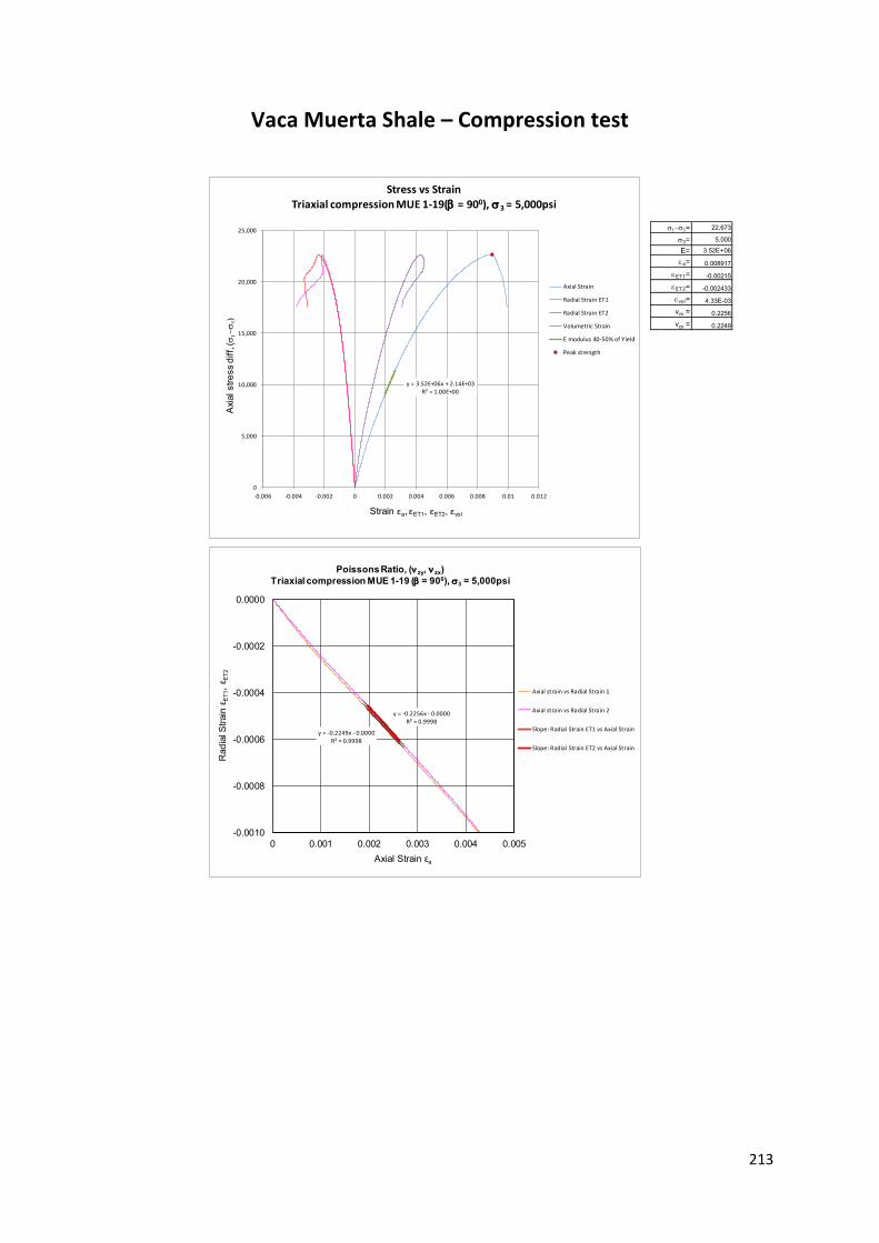
213
Vaca Muerta Shale – Compression test
13= 22,673
3= 5,000
E= 3.52E+06
a= 0.008917
ET1= -0.00215
ET2= -0.002433
vol= 4.33E-03
vzx = 0.2256
vzy = 0.2249
y = 3.52E+06x + 2.14E+03R² = 1.00E+00
0
5,000
10,000
15,000
20,000
25,000
-0.006 -0.004 -0.002 0 0.002 0.004 0.006 0.008 0.01 0.012
Axia
l str
ess d
iff,
(1
3
Strain εa, εET1, εET2, εvol
Stress vs StrainTriaxial compression MUE 1-19( = 900), 3 = 5,000psi
Axial Strain
Radial Strain ET1
Radial Strain ET2
Volumetric Strain
E modulus 40-50% of Yield
Peak strength
y = -0.2249x - 0.0000R² = 0.9998
y = -0.2256x - 0.0000R² = 0.9998
-0.0010
-0.0008
-0.0006
-0.0004
-0.0002
0.0000
0 0.001 0.002 0.003 0.004 0.005
Rad
ial S
train
εE
T1, ε E
T2
Axial Strain εa
Axial strain vs Radial Strain 1
Axial strain vs Radial Strain 2
Slope: Radial Strain ET1 vs Axial Strain
Slope: Radial Strain ET2 vs Axial Strain
Poissons Ratio, (n zy, n zx)
Triaxial compression MUE 1-19 ( = 900), 3 = 5,000psi

214
Vaca Muerta Shale – Compression test
13= 49,963
3= 20,000
E= 2.35E+06
a= 0.067036
ET1= -0.022181
ET2= -0.022008
vol= 2.28E-02
vzx = 0.1605
vzy = 0.1474
y = 2.35E+06x + 2.34E+03R² = 9.98E-01
0
10,000
20,000
30,000
40,000
50,000
60,000
-0.06 -0.04 -0.02 0 0.02 0.04 0.06 0.08 0.1
Axia
l str
ess d
iff,
(1
3
Strain εa, εET1, εET2, εvol
Stress vs StrainTriaxial compression MUE 1-3( = 00), 3 = 5,000psi
Axial Strain
Radial Strain ET1
Radial Strain ET2
Volumetric Strain
E modulus 40-50% of Yield
Peak strength
y = -0.1605x - 0.0000R² = 0.9993
y = -0.1474x - 0.0000R² = 0.9994
-0.0005
-0.0004
-0.0003
-0.0002
-0.0001
0.0000
0 0.001 0.002 0.003 0.004
Rad
ial S
train
εE
T1, ε E
T2
Axial Strain εa
Axial strain vs Radial Strain 1
Axial strain vs Radial Strain 2
Slope: Radial Strain ET1 vs Axial Strain
Slope: Radial Strain ET2 vs Axial Strain
Poissons Ratio, (n zy, n zx)
Triaxial compression MUE 1-3 ( = 00), 3 = 5,000psi

215
Vaca Muerta Shale – Compression test
13= 41,119
3= 20,000
E= 3.01E+06
a= 0.058103
ET1= -0.021896
ET2= -0.037697
vol= -1.49E-03
vzx = 0.1909
vzy = 0.1849
y = 3.01E+06x + 1.15E+03R² = 9.98E-01
0
5,000
10,000
15,000
20,000
25,000
30,000
35,000
40,000
45,000
-0.06 -0.04 -0.02 0 0.02 0.04 0.06 0.08 0.1
Axia
l str
ess d
iff,
(1
3
Strain εa, εET1, εET2, εvol
Stress vs StrainTriaxial compression MUE 1-12( = 600), 3 = 20,000psi
Axial Strain
Radial Strain ET1
Radial Strain ET2
Volumetric Strain
E modulus 40-50% of Yield
Peak strength
y = -0.1909x - 0.0000R² = 0.9997
y = -0.1849x - 0.0000R² = 0.9986
-0.0006
-0.0005
-0.0004
-0.0003
-0.0002
-0.0001
0.0000
0 0.001 0.002 0.003 0.004 0.005
Rad
ial S
train
εE
T1, ε E
T2
Axial Strain εa
Axial strain vs Radial Strain 1
Axial strain vs Radial Strain 2
Slope: Radial Strain ET1 vs Axial Strain
Slope: Radial Strain ET2 vs Axial Strain
Poissons Ratio, (n zy, n zx)
Triaxial compression MUE 1-12 ( = 600), 3 = 20,000psi

216
Vaca Muerta Shale – Compression test
13= 47,894
3= 20,000
E= 4.44E+06
a= 0.081562
ET1= -0.059534
ET2= -0.042261
vol= -2.02E-02
vzx = 0.2030
vzy = 0.2499
y = 4.44E+06x + 5.90E+02R² = 9.96E-01
0
10,000
20,000
30,000
40,000
50,000
60,000
-0.1 -0.08 -0.06 -0.04 -0.02 0 0.02 0.04 0.06 0.08 0.1
Axia
l str
ess d
iff,
(1
3
Strain εa, εET1, εET2, εvol
Stress vs StrainTriaxial compression MUE 1-20 ( = 900), 3 = 20,000psi
Axial Strain
Radial Strain ET1
Radial Strain ET2
Volumetric Strain
Series3
Peak strength
y = -0.2499x - 0.0000R² = 0.9962
y = -0.2030x - 0.0000R² = 0.9933
-0.0005
-0.0004
-0.0003
-0.0002
-0.0001
0.0000
0 0.001 0.002 0.003
Rad
ial S
train
εE
T1, ε E
T2
Axial Strain εa
Axial strain vs Radial Strain 1
Axial strain vs Radial Strain 2
Slope: Radial Strain ET1 vs Axial Strain
Slope: Radial Strain ET2 vs Axial Strain
Poissons Ratio, (n zy, n zx)
Triaxial compression MUE 1-20 ( = 900), 3 = 20,000psi
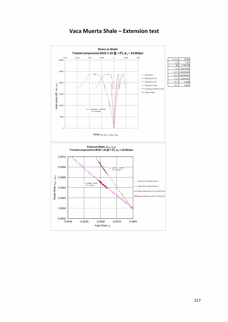
217
Vaca Muerta Shale – Extension test
13= 23,802
3= 1,161
E= 4.74E+06
a= -0.00775522
ET1= 0.003801683
ET2= 0.001848205
vol= -0.00210533
vzx = 0.2666
vzy = 0.4501
y = -4.74E+06x + 1.89E+03R² = 9.92E-01
0
5000
10000
15000
20000
25000
30000
-0.02 -0.015 -0.01 -0.005 0 0.005 0.01A
xia
l str
ess d
iff,
-(
1
3
Strain εa, εET1, εET2, εvol
Stress vs StrainTriaxial compression MUE 1-24 ( = 00), 1 = 24,963psi
Axial Strain
Radial Strain ET1
Radial Strain ET2
Volumetric Strain
E modulus 40-50% of Yield
Peak strength
y = -0.4501x - 0.0000R² = 0.9769
y = -0.2666x - 3E-05R² = 0.9123
-0.0002
0.0000
0.0002
0.0004
0.0006
0.0008
0.0010
-0.0040 -0.0030 -0.0020 -0.0010 0.0000
Rad
ial S
train
εE
T1, ε E
T2
Axial Strain εa
Axial strain vs Radial Strain 1
Axial strain vs Radial Strain 2
Slope: Radial Strain ET1 vs Axial Strain
Slope: Radial Strain ET2 vs Axial Strain
Poissons Ratio, (n zy, n zx)
Triaxial compression MUE 1-24 ( = 00), 3 = 24,963psi

218
Vaca Muerta Shale – Extension test
13= 19,510
3= 3,109
E= 3.25E+06
a= -0.00820747
ET1= 0.002294112
ET2= 0.004119127
vol= -0.00179423
vzx = 0.2289
vzy = 0.4239
y = -3.25E+06x + 2.04E+03R² = 9.97E-01
0
5000
10000
15000
20000
25000
-0.012 -0.01 -0.008 -0.006 -0.004 -0.002 0 0.002 0.004 0.006
Axia
l str
ess d
iff,
-(
1
3
Strain εa, εET1, εET2, εvol
Stress vs StrainTriaxial compression MUE 1-25 ( = 600), 1 = 22,619psi
Axial Strain
Radial Strain ET1
Radial Strain ET2
Volumetric Strain
E modulus 40-50% of Yield
Peak strength
y = -0.2289x - 0.0001R² = 0.9492
y = -0.4239x - 7E-05R² = 0.9837
-0.0002
0.0000
0.0002
0.0004
0.0006
0.0008
0.0010
-0.0040 -0.0030 -0.0020 -0.0010 0.0000
Rad
ial S
train
εE
T1, ε E
T2
Axial Strain εa
Axial strain vs Radial Strain 1
Axial strain vs Radial Strain 2
Slope: Radial Strain ET1 vs Axial Strain
Slope: Radial Strain ET2 vs Axial Strain
Poissons Ratio, (n zy, n zx)
Triaxial compression MUE 1-25 ( = 600), 3 = 22,619psi

219
B1 JPW model objective function
% Matlab code - Objective function (Jaeger plane of weakness for 1 > 2 = 3)
% This Matlab code is used to input strength data, and model RMSE is calculated for the
% combination of strength parameters taken from the main loop (B2). The strength
% parameters with least RMSE is determined from the main Loop (B2) and used to
calculate % strength 1 and plotted against data sets for comparison.
function Error=Objectivefun(x,options); format compact Data = ... [ ... 0 90 6140 0 60 1811 0 45 6874 0 45 5653 0 30 6577 0 0 16466 1000 90 21371 1000 60 6672 1000 45 8021 1000 30 13321 1000 0 18106 3000 90 28988 3000 75 19834 3000 60 13751 3000 45 15678 3000 30 19367 3000 30 17500 3000 15 17103 3000 15 20956 3000 0 30060 6000 90 37437 6000 60 20330 6000 45 22722 6000 30 25984 6000 30 24026 6000 30 23468 6000 20 30920 6000 0 36951 10000 90 47097 10000 75 39812 10000 60 33197 10000 45 32556 10000 30 36198 10000 15 42278 10000 10 38263 10000 0 42614 ]; t = Data(:,2); sig1 = Data(:,3); sig3 = Data(:,1);
So=x(1);

220
fo=x(2); Sw=x(3); fw=x(4);
sig1T= 2*So*((cos(fo*pi/180))./(1-
(sin(fo*pi/180))))+sig3*((1+(sin(fo*pi/180)))./(1-(sin(fo*pi/180))))+0*t;
sig1W=sig3+(2*(Sw+sig3*(tan(fw*pi/180))))./((1-
((tan(fw*pi/180))./(tan(t*pi/180)))).*(sin((2*t)*pi/180)));
for i=1:length(sig1W) if (sig1W(i)<0) sig1W(i)=1.0E50; end end
sig1T=min(sig1T,sig1W);
Error=((1/36)*sum((sig1-sig1T).^2)).^0.5
if (options(1)==1)
%Start plot for sig3=10kpsi tt=0:1:90; sig1_10k= 2*So*((cos(fo*pi/180))./(1-
(sin(fo*pi/180))))+10000*((1+(sin(fo*pi/180)))./(1-(sin(fo*pi/180))))+0*tt; sig1W_10k=10000+(2*(Sw+10000*(tan(fw*pi/180))))./((1-
((tan(fw*pi/180))./(tan(tt*pi/180)))).*(sin((2*tt)*pi/180))); for i=1:length(sig1W_10k); if (sig1W_10k(i)<0); sig1W_10k(i)=1.0E50; end end sig1_10k=min(sig1_10k,sig1W_10k);
%Start plot for sig3=6kpsi sig1_6k= 2*So*((cos(fo*pi/180))./(1-
(sin(fo*pi/180))))+6000*((1+(sin(fo*pi/180)))./(1-(sin(fo*pi/180))))+0*tt; sig1W_6k=6000+(2*(Sw+6000*(tan(fw*pi/180))))./((1-
((tan(fw*pi/180))./(tan(tt*pi/180)))).*(sin((2*tt)*pi/180))); for i=1:length(sig1W_6k); if (sig1W_6k(i)<0); sig1W_6k(i)=1.0E50; end end sig1_6k=min(sig1_6k,sig1W_6k);
%Start plot for sig3=3kpsi sig1_3k= 2*So*((cos(fo*pi/180))./(1-
(sin(fo*pi/180))))+3000*((1+(sin(fo*pi/180)))./(1-(sin(fo*pi/180))))+0*tt; sig1W_3k=3000+(2*(Sw+3000*(tan(fw*pi/180))))./((1-
((tan(fw*pi/180))./(tan(tt*pi/180)))).*(sin((2*tt)*pi/180))); for i=1:length(sig1W_3k); if (sig1W_3k(i)<0); sig1W_3k(i)=1.0E50; end end sig1_3k=min(sig1_3k,sig1W_3k);
%Start plot for sig3=1kpsi

221
sig1_1k= 2*So*((cos(fo*pi/180))./(1-
(sin(fo*pi/180))))+1000*((1+(sin(fo*pi/180)))./(1-(sin(fo*pi/180))))+0*tt; sig1W_1k=1000+(2*(Sw+1000*(tan(fw*pi/180))))./((1-
((tan(fw*pi/180))./(tan(tt*pi/180)))).*(sin((2*tt)*pi/180))); for i=1:length(sig1W_1k); if (sig1W_1k(i)<0); sig1W_1k(i)=1.0E50; end end sig1_1k=min(sig1_1k,sig1W_1k);
%Start plot for sig3=UCS sig1_UCS= 2*So*((cos(fo*pi/180))./(1-
(sin(fo*pi/180))))+0*((1+(sin(fo*pi/180)))./(1-(sin(fo*pi/180))))+0*tt; sig1W_UCS=0+(2*(Sw+0*(tan(fw*pi/180))))./((1-
((tan(fw*pi/180))./(tan(tt*pi/180)))).*(sin((2*tt)*pi/180))); for i=1:length(sig1W_UCS); if (sig1W_UCS(i)<0); sig1W_UCS(i)=1.0E50; end end sig1_UCS=min(sig1_UCS,sig1W_UCS);
plot(t(1:6),sig1(1:6),'r*'); plot(t(7:11),sig1(7:11),'co'); plot(t(12:20),sig1(12:20),'go'); plot(t(21:28),sig1(21:28),'bo'); plot(t(29:36),sig1(29:36),'ro');
hold on; plot (tt,sig1_10k,'-r'); plot (tt,sig1_6k,'-b'); plot (tt,sig1_3k,'-g'); plot (tt,sig1_1k,'-c'); plot (tt,sig1_UCS,'-r'); end
end

222
B2 JPW model main loop
% Matlab code - MainLoop (Jaeger plane of weakness for 1 > 2 = 3)
% This Matlab code is where strength parameters are input iteratively to be used in B1 clc tic
nN=20; Y(1:nN*nN*nN*nN*nN*nN+10)=10^20; for iSo=1:1:nN for ifo=1:1:nN for iSw=1:1:nN for ifw=1:1:nN
So=50*(iSo)+3300; % 3.3k<So<4.3k ; 0.05kpsi No.n fo=0.1*(ifo)+28; % 28.1deg<fo<30deg ; 0.1deg Sw=50*(iSw)+2000; % 2.02k<Sw<3k ; 0.05kpsi fw=0.1*(ifw)+23.5; % 23.6deg<fw<24.5deg ; 0.1deg
% Different intervals applied here
% So=5000*(iSo)-5000; % 0k<So<95k ; 5kpsi No.1 % fo=5*(ifo)-5; % 0deg<fo<95deg ; 5deg % Sw=5000*(iSw)-5000; % 0k<Sw<95k ; 5kpsi % fw=5*(ifw)-5; % 0deg<fw<95deg ; 5deg
xxxx=[So fo Sw fw]; initialStepSize=0.1*abs(xxxx)+100;% changed the step size
index=iSo*nN*nN*nN+ifo*nN*nN+iSw*nN+ifw; X6Dim(index,1:4)=xxxx; Ytmp=Objectivefun(xxxx,[0,0]); Y(index)=Ytmp;
end end end end Ymin=min(Y) indexminAll=find(Y==Ymin, 1 ); indexmin=min(find(Y==Ymin)); Objectivefun(X6Dim(indexmin,1:4),[1,1]);
So=X6Dim(indexmin,1) fo=X6Dim(indexmin,2) Sw=X6Dim(indexmin,3) fw=X6Dim(indexmin,4)
xxxx=[So fo Sw fw]; Objectivefun(xxxx,[1,1]); toc

223
B3 Pariseau model objective function
% Matlab code – Objective function (Pariseau model for 1 > 2 = 3)
% This Matlab code is used to input strength data, and Pariseau model RMSE is calculated.
% The strength parameters F, G, U, V and M determined with least RMSE from the main
Loop % (B4) is then used to calculate strength 1 and this is plotted against data sets for
% comparison
function Error=Objectivefun(x,options); format compact Data = ... [ ... 10000 90 32614 10000 80 28263 10000 75 32278 10000 60 26198 10000 45 22556 10000 30 23197 10000 15 29812 10000 0 37097 6000 90 30951 6000 70 24920 6000 60 19984 6000 60 17468 6000 60 18026 6000 45 16722 6000 30 14330 6000 0 31437 3000 90 27060 3000 75 14103 3000 75 17956 3000 60 16367 3000 60 14500 3000 45 12678 3000 30 10751 3000 15 16834 3000 0 25988 1000 90 17106 1000 60 12321 1000 45 7021 1000 30 5672 1000 0 20371 0 90 16466 0 60 6577 0 45 5653 0 45 6874 0 30 1811 0 0 6140]; t = Data(:,2); sig13 = Data(:,3); sig3 = Data(:,1);
F=1.0/(x(1)*(x(1)));

224
G=1.0/(x(2)*(x(2))); U=1.0/x(3); V=1.0/x(4); M=1.0/(x(5)*(x(5)));
xPos=((F*(sin(t*pi/180)).^4)+G*((cos(t*pi/180)).^4+((cos(2*t*pi/180)).^2))+
0.25*M*((sin(2*t*pi/180))).^2);
Error=((1/36)*sum((sig13-
((1+(U+2*V)*sig3)./((((F*(sin(t*pi/180)).^4)+G*((cos(t*pi/180)).^4+((cos(2*
t*pi/180)).^2))+0.25*M*((sin(2*t*pi/180))).^2)).^0.5... -(U*(cos(t*pi/180)).^2+V*(sin(t*pi/180)).^2)))).^2)).^0.5
if (options(1)>0 & xPos>0) tt=0:1:90;
sig13_10k=((1+(U+2*V)*10000)./((((F*(sin(tt*pi/180)).^4)+G*((cos(tt*pi/180)
).^4+((cos(2*tt*pi/180)).^2))+0.25*M*((sin(2*tt*pi/180))).^2)).^0.5... -(U*(cos(tt*pi/180)).^2+V*(sin(tt*pi/180)).^2)));
sig13_6k=((1+(U+2*V)*6000)./((((F*(sin(tt*pi/180)).^4)+G*((cos(tt*pi/180)).
^4+((cos(2*tt*pi/180)).^2))+0.25*M*((sin(2*tt*pi/180))).^2)).^0.5... -(U*(cos(tt*pi/180)).^2+V*(sin(tt*pi/180)).^2)));
sig13_3k=((1+(U+2*V)*3000)./((((F*(sin(tt*pi/180)).^4)+G*((cos(tt*pi/180)).
^4+((cos(2*tt*pi/180)).^2))+0.25*M*((sin(2*tt*pi/180))).^2)).^0.5... -(U*(cos(tt*pi/180)).^2+V*(sin(tt*pi/180)).^2)));
sig13_1k=((1+(U+2*V)*1000)./((((F*(sin(tt*pi/180)).^4)+G*((cos(tt*pi/180)).
^4+((cos(2*tt*pi/180)).^2))+0.25*M*((sin(2*tt*pi/180))).^2)).^0.5... -(U*(cos(tt*pi/180)).^2+V*(sin(tt*pi/180)).^2)));
sig13_UCS=((1+(U+2*V)*0)./((((F*(sin(tt*pi/180)).^4)+G*((cos(tt*pi/180)).^4
+((cos(2*tt*pi/180)).^2))+0.25*M*((sin(2*tt*pi/180))).^2)).^0.5... -(U*(cos(tt*pi/180)).^2+V*(sin(tt*pi/180)).^2)));
plot(t,sig13,'bo'); hold on; plot (tt,sig13_10k,'rx'); plot (tt,sig13_6k,'g*'); plot (tt,sig13_3k,'bx'); plot (tt,sig13_1k,'go'); plot (tt,sig13_UCS,'r*'); end
end

225
B4 Pariseau model main Loop
% Matlab code - MainLoop (Pariseau model for 1 > 2 = 3)
% This Matlab code is where parameters F, G, U, V and M are input iteratively to use in B3 clear clc tic
nN=12; Y(1:nN*nN*nN*nN*nN*nN+10)=10^12; for iF=1:1:nN for iG=1:1:nN for iU=1:1:nN for iV=1:1:nN for iM=1:1:nN
FinvSqrt=100*(iF)+19900; % 20.0k<F<21.1k ; 0.1kpsi interval No. i-Trials GinvSqrt=100*(iG)+8900; % 9.0k<G<10.1k ; 0.1kpsi interval Uinv=100*(iU)+12400; % 12.5k<U<13.6k ; 0.1kpsi interval Vinv=100*(iV)+20900; % 21.0k<V<22.1k ; 0.1kpsi interval MinvSqrt=100*(iM)+1900; % 2.0<M<3.1k ; 0.1kpsi interval
xxxx=[FinvSqrt GinvSqrt Uinv Vinv MinvSqrt]; initialStepSize=0.1*abs(xxxx)+100;% changed the step size
index=iF*nN*nN*nN*nN+iG*nN*nN*nN+iU*nN*nN+iV*nN+iM; X6Dim(index,1:5)=xxxx; Ytmp=Objectivefun(xxxx,[0,0]); Y(index)=Ytmp;
end end end end end
Ymin=min(Y) indexminAll=find(Y==Ymin, 1 ) indexmin=min(find(Y==Ymin)); Objectivefun(X6Dim(indexmin,1:5),[1,1])
FinvSqrt=X6Dim(indexmin,1) GinvSqrt=X6Dim(indexmin,2) Uinv=X6Dim(indexmin,3) Vinv=X6Dim(indexmin,4) MinvSqrt=X6Dim(indexmin,5) xxxx=[FinvSqrt GinvSqrt Uinv Vinv MinvSqrt]; Objectivefun(xxxx,[1,1])
Toc

226
B5 True-triaxial Pariseau model objective
function
% Matlab code – Objective function (Pariseau model for 1 > 2 > 3)
% This Matlab code is used to input strength data, and Pariseau model RMSE is calculated.
% The strength parameters F, G, U, V and M determined from the main Loop (B6) with
least
% RMSE is then used to calculate strength 1 and plotted against data sets for comparison
function Error=Objectivefun(x,options); format compact Data = ... [ ... 0 0 60 8557 0 0 0 60 10298 0 0 3626 60 22336 3626 0 7252 60 35389 7252 0 10878 60 47572 10878 45 0 60 9572 0 45 0 60 9863 0 45 3626 60 24801 3626 45 7252 60 33794 7252 45 7252 60 35244 7252 45 7252 60 35389 7252 45 10878 60 47137 10878 45 10878 60 48733 10878 0 0 0 21321 0 0 0 0 21611 0 0 3626 0 42641 3626 0 7252 0 55840 7252 0 10878 0 72664 10878 0 7252 60 35389 7252 0 7252 60 32633 12328 0 7252 60 29878 14504 0 7252 60 30168 17550 0 7252 60 34809 19290 0 7252 60 32633 24076 45 7252 60 33794 7252 45 7252 60 35389 7252 45 7252 60 35824 7252 45 7252 60 39595 8122 45 7252 60 42061 10153 45 7252 60 42641 12473 45 7252 60 43511 14069 45 7252 60 43221 14069 45 7252 60 50183 17550 45 7252 60 48588 17550 45 7252 60 46122 20885 45 7252 60 44672 22626 45 7252 60 46267 24221 45 7252 60 50183 24366 45 7252 60 44091 26107

227
45 7252 60 46412 29443 45 7252 60 54534 29443 45 7252 60 45397 32924 90 7252 60 31763 7252 90 7252 60 35389 7252 90 7252 60 45107 12473 90 7252 60 46122 14069 90 7252 60 57580 17550 90 7252 60 64542 22481 90 7252 60 70778 22626 0 7252 0 55840 7252 0 7252 0 64687 10298 0 7252 0 64832 10733 0 7252 0 70488 10878 0 7252 0 72809 14939 0 7252 0 76580 16679 0 7252 0 77015 21466 0 7252 0 78320 22626 0 7252 0 83687 27847 0 7252 0 81656 32924 0 7252 0 79191 36114 0 7252 0 81511 38000 0 7252 0 81946 45832 ];
L = Data (:,1); sig3 = Data(:,2); t = Data(:,3); sig1 = Data(:,4); sig2 = Data(:,5);
F=1.0/(x(1)*(x(1))); G=1.0/(x(2)*(x(2))); U=1.0/x(3); V=1.0/x(4); M=1.0/(x(5)*(x(5)));
xPos=((F*(sin(t*pi/180)).^4)+G*((cos(t*pi/180)).^4+((cos(2*t*pi/180)).^2))+
0.25*M*((sin(2*t*pi/180))).^2);
sig22=(cos(t*pi/180)).^2.*((sig2.*(cos(L*pi/180)).^2)+sig3.*(sin(L*pi/180))
.^2)+sig1.*(sin(t*pi/180)).^2;
sig33 = (((sig2.*(sin(L*pi/180)).^2) + sig3.*((cos(L*pi/180)).^2)));
sig11=(sin(t*pi/180)).^2.*((sig2.*(cos(L*pi/180)).^2)+sig3.*(sin(L*pi/180))
.^2)+sig1.*(cos(t*pi/180)).^2;
sig23 =(cos(t*pi/180)).*(cos(L*pi/180)).*(sin(L*pi/180)).*(sig3-sig2);
sig31 =(sin(t*pi/180)).*(cos(L*pi/180)).*(sin(L*pi/180)).*(sig3-sig2);
sig12=(cos(t.*pi/180)).*(sin(t.*pi/180)).*((sig2.*(cos(L.*pi/180)).^2)+sig3
.*(sin(L.*pi/180)).^2-sig1);
Error=((1/62)*sum((1-(((F*(sig22-sig33).^2+G*((sig33-sig11).^2+(sig11-
sig22).^2)+(2*G+4*F)*sig23.^2+M*(sig31.^2+sig12.^2)).^0.5-
(U*sig11+V*(sig22+sig33))))).^2)).^0.5
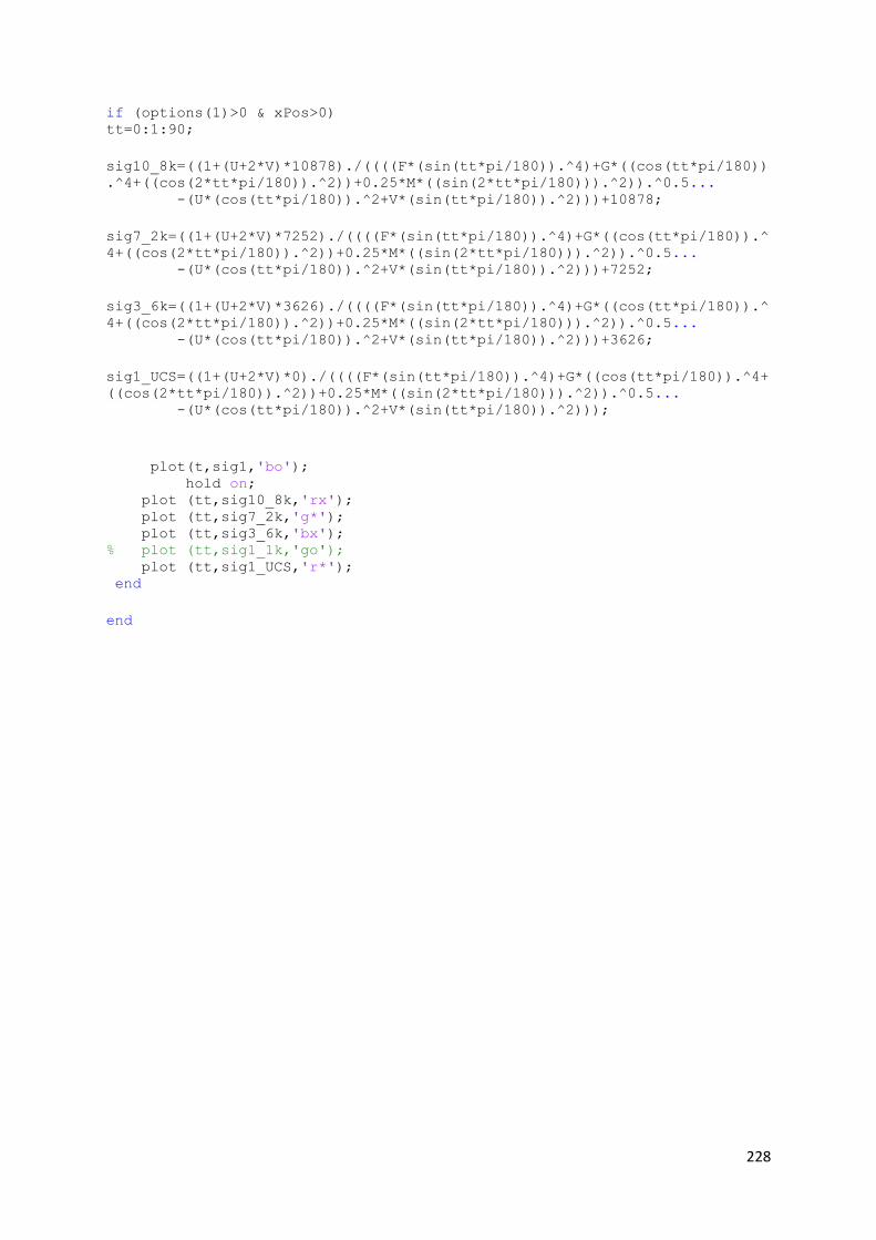
228
if (options(1)>0 & xPos>0) tt=0:1:90;
sig10_8k=((1+(U+2*V)*10878)./((((F*(sin(tt*pi/180)).^4)+G*((cos(tt*pi/180))
.^4+((cos(2*tt*pi/180)).^2))+0.25*M*((sin(2*tt*pi/180))).^2)).^0.5... -(U*(cos(tt*pi/180)).^2+V*(sin(tt*pi/180)).^2)))+10878;
sig7_2k=((1+(U+2*V)*7252)./((((F*(sin(tt*pi/180)).^4)+G*((cos(tt*pi/180)).^
4+((cos(2*tt*pi/180)).^2))+0.25*M*((sin(2*tt*pi/180))).^2)).^0.5... -(U*(cos(tt*pi/180)).^2+V*(sin(tt*pi/180)).^2)))+7252;
sig3_6k=((1+(U+2*V)*3626)./((((F*(sin(tt*pi/180)).^4)+G*((cos(tt*pi/180)).^
4+((cos(2*tt*pi/180)).^2))+0.25*M*((sin(2*tt*pi/180))).^2)).^0.5... -(U*(cos(tt*pi/180)).^2+V*(sin(tt*pi/180)).^2)))+3626;
sig1_UCS=((1+(U+2*V)*0)./((((F*(sin(tt*pi/180)).^4)+G*((cos(tt*pi/180)).^4+
((cos(2*tt*pi/180)).^2))+0.25*M*((sin(2*tt*pi/180))).^2)).^0.5... -(U*(cos(tt*pi/180)).^2+V*(sin(tt*pi/180)).^2)));
plot(t,sig1,'bo'); hold on; plot (tt,sig10_8k,'rx'); plot (tt,sig7_2k,'g*'); plot (tt,sig3_6k,'bx'); % plot (tt,sig1_1k,'go'); plot (tt,sig1_UCS,'r*'); end
end

229
B6 True-triaxial Pariseau model main
loop
% Matlab code - MainLoop (Pariseau model for 1 > 2 > 3) % This Matlab code is where parameters F, G, U, V and M are input iteratively to use in B5
clear clc tic
nN=12; Y(1:nN*nN*nN*nN*nN*nN+10)=10^12; for iF=1:1:nN for iG=1:1:nN for iU=1:1:nN for iV=1:1:nN for iM=1:1:nN
FinvSqrt=-1000*(iF)-34000; % -46k<F<-57k ; 1kpsi interval No. 30 GinvSqrt=2000*(iG)+50000; % 52<G<74k ; 2kpsi interval Uinv=5000*(iU)+75000; % 80k<U<135k ; 5kpsi interval Vinv=5000*(iV)+75000; % 80k<V<135k ; 5kpsi interval MinvSqrt=500*(iM)+8000; % 8.5<M<14k ; 0.5kpsi interval
% FinvSqrt=-1000*(iF)-45000; % -46k<F<-57k ; 1kpsi interval No. 29 % GinvSqrt=2000*(iG)+50000; % 52<G<74k ; 2kpsi interval % Uinv=5000*(iU)+75000; % 80k<U<135k ; 5kpsi interval % Vinv=5000*(iV)+75000; % 80k<V<135k ; 5kpsi interval % MinvSqrt=1000*(iM)+9000; % 10<M<22k ; 1kpsi interval % ….
% iteration…. No. 2 to 29 % ….
% FinvSqrt=20000*(iF-nN/2); % -100k<F<120k ; 20kpsi interval No. 2 % GinvSqrt=10000*(iG)-10000; % 0<G<110k ; 10kpsi interval % Uinv=20000*(iU)-20000; % 0k<U<220k ; 20kpsi interval % Vinv=20000*(iV)-20000; % 0k<V<220k ; 20kpsi interval % MinvSqrt=5000*(iM)-10000; % 0<M<60k ; 5kpsi interval
% FinvSqrt=20000*(iF-nN/2); % -100k<F<120k ; 20kpsi interval No. 1 % GinvSqrt=10000*(iG)-10000; % 0<G<110k ; 10kpsi interval % Uinv=10000*(iU)-10000; % 0k<U<110k ; 5kpsi interval % Vinv=10000*(iV)-10000; % 0k<V<110k ; 5kpsi interval % MinvSqrt=10000*(iM)-10000; % 0<M<100k ; 10kpsi interval
xxxx=[FinvSqrt GinvSqrt Uinv Vinv MinvSqrt]; initialStepSize=0.1*abs(xxxx)+100;% changed the step size
index=iF*nN*nN*nN*nN+iG*nN*nN*nN+iU*nN*nN+iV*nN+iM; X6Dim(index,1:5)=xxxx; Ytmp=Objectivefun(xxxx,[0,0]); Y(index)=Ytmp;
end

230
end end end end
Ymin=min(Y)
indexminAll=find(Y==Ymin, 1 ) indexmin=min(find(Y==Ymin)); Objectivefun(X6Dim(indexmin,1:5),[1,1])
FinvSqrt=X6Dim(indexmin,1) GinvSqrt=X6Dim(indexmin,2) Uinv=X6Dim(indexmin,3) Vinv=X6Dim(indexmin,4) MinvSqrt=X6Dim(indexmin,5) xxxx=[FinvSqrt GinvSqrt Uinv Vinv MinvSqrt]; Objectivefun(xxxx,[1,1])
toc

231
B7 True-triaxial Pariseau model strength
1 prediction
% The Objective of this Matlab code is to determine strength 1 using the parameters F, G,
U, % V and M determined for least RMSE from B5 and B6. The Pariseau model strength 1
is
% determined as a function of 2, 3, and , for defined parameters F, G, U, V and M.
The
% final output is a plot of 1 vs. 2 for defined 3, and
clc; clear all; tic
F=4.7259E-10; G=4.34028E-10; U=0.0000125; V=7.40741E-06; M=1.23457E-08;
firstPass = 1;
for sig2=7.251e3:2e3:150e3
beta=60; % Input angle beta here t=90-beta;
omega=0; % Input angle omega here L=90-omega;
sig3=7252;
sig1 = sym('sig1','positive');
sig22=(cos(t*pi/180)).^2.*((sig2.*(cos(L*pi/180)).^2)+sig3.*(sin(L*pi/180))
.^2)+sig1.*(sin(t*pi/180)).^2;
sig33 = (((sig2*(sin(L*pi/180)).^2) + sig3*((cos(L*pi/180)).^2)));
sig11=(sin(t*pi/180)).^2.*((sig2*(cos(L*pi/180)).^2)+sig3*(sin(L*pi/180)).^
2)+sig1*(cos(t*pi/180)).^2;
sig23 =(cos(t*pi/180)).*(cos(L*pi/180)).*(sin(L*pi/180))*(sig3-sig2);
sig31 =(sin(t*pi/180)).*(cos(L*pi/180)).*(sin(L*pi/180))*(sig3-sig2);

232
sig12=(cos(t*pi/180)).*(sin(t*pi/180)).*((sig2*(cos(L*pi/180)).^2)+sig3*(si
n(L*pi/180)).^2-sig1);
sig1_calc = solve(((F*(sig22-sig33).^2+G*((sig33-sig11).^2+(sig11-
sig22).^2)+(2*G+4*F)*sig23.^2+M*(sig31.^2+sig12.^2)).^0.5-
(U*sig11+V*(sig22+sig33))-1), sig1);
sig1_calc = max(double(sig1_calc))
sig2 if( firstPass == 1) sig2_calc = sig2; sig1_calc_toPlot = sig1_calc; firstPass = 0; else sig2_calc=[sig2_calc,sig2] ; sig1_calc_toPlot = [sig1_calc_toPlot,sig1_calc]; end
plot (sig2_calc,sig1_calc_toPlot,'bx');
title('sig1 vs sig2'); xlabel('sig2'); ylabel('sig1'); axis([0 140e3 0 140e3]);
end
toc

233
B8 True-triaxial JPW model strength 1
prediction
% Matlab code – True-triaxial JPW model
% This Matlab code is used to compute strength 1 using Coulomb strength parameters So,
% o, Sw and w, for defined 3, and
clc tic
beta= 61.4 ;% % Input angle beta here
omega=32.8 ;% % Input angle omega here n=(cos(omega*pi/180));%n=(cos(Lambda*pi/180)) ; n=>omega=w=direction l=(cos(beta*pi/180));%n=(cos(Lambda*pi/180)) ; l=>bedding angle
S=4101.2% "Sw=1694.8"; "So=4101.2";
phi=32.8% "fw=25.8" ; "fo=32.8";
u=(tan(phi*pi/180));%tan phi
firstPass = 1;
for sig2=7212:0.5e3:120e3; sig3=7312; sig1 = sym('sig1','positive'); sig=sig2-(sig2-sig3)*n^2-(sig2-sig1)*l^2; Tau=(n^2*(sig1-sig3)*(sig2-sig3)-(sig1-sig)*(sig2-sig))^0.5; sig1_calc = solve((Tau-S-u*sig), sig1); sig1_calc = max(double(sig1_calc))
sig2 if( firstPass == 1) sig2_calc = sig2; sig1_calc_toPlot = sig1_calc; firstPass = 0; else sig2_calc=[sig2_calc,sig2] ; sig1_calc_toPlot = [sig1_calc_toPlot,sig1_calc]; end
plot (sig2_calc,sig1_calc_toPlot,'bx');
title('sig1 vs sig2'); xlabel('sig2'); ylabel('sig1'); axis([0 120e3 0 120e3]);
end toc

234
C Differentiate Coulomb criterion for min
The Coulomb criterion for shear stress acting along the plane is a function of cohesion S, friction
angle and normal stress n. For shear fracture of rock to occur, the Coulomb criterion needs to be
satisfied, and the mathematical representation of the Coulomb criterion is
| | . C.1.1
The shear and normal stress can be determined using the Mohr circle and expressed as a function of
principal stresses using maximum shear stress m and mean normal stress m as follows
| |, C.1.2
. C.1.3
Replacing the shear and normal stressn into the Coulomb criterion gives the general Coulomb
criterion for shear failure at an arbitrary angle as
(
) [ (
)]. C.1.4
The above eqn. C.1.4 is also the plane of weakness criterion derived by Jaeger (1960) using the
Coulomb criterion. To determine the Coulomb criterion (i.e., angle where minimum shear strength
occurs), Coulomb differentiated the general solution in Eqn. C.1.4 with respect to angle as follows
{(
) [ (
)]}. C.1.5
Since the numerator is a constant, replace this with a new term k:
{( ) [ (
)]}, C.1.6
( ) ( ) ( ) . C.1.7
At minimum shear, the slope of the function m is zero, hence
( ) ( ) ( ) =0. C.1.8
By equating ( ) , the solution for minimum shear occurs at
Alternatively, using trigonometry and rearranging Eqn. C.1.8
( ) ( ) ( ) , C.1.9
( ) ( ) ( ) , C.1.10

235
( ) [(
) ( )] , C.1.11
( ) ( ) ( ) ( ) , C.1.12
( ) ( ) ( ) ( ) . C.1.13
Equation C.1.13 solved for the prescribed condition
( ) , C.1.14
( ⁄ ). C.1.15
Equation C.1.15 is the same equation shown in Jaeger et al. (2007, pg. 104). Using shifts or
periodicity eqn. C.1.15 is
( ( )⁄ ), C.1.16
( ), C.1.17
. C.1.18
The above Coulomb solution is the angle where shear failure of intact rock occurs, and depending on
orientation and periodicity, Eqn. C.1.18 is also sometimes written as
. C.1.19

236
D1 Data from literature - various
anisotropic rocks
Note: 1 and 3 are in units of psi; angle is as defined for triaxial compression tests in
chapter 5
3 β 1 3 β 1 3 β 1 3 β 1 3 β 1
0 0 21,509 508 90 19,245 5,000 90 50,244 1,000 90 36,553 1,000 90 21,556
0 15 10,182 508 75 7,551 5,000 80 39,361 1,000 75 30,060 1,000 80 19,227
0 30 5,279 508 60 3,176 5,000 70 25,072 1,000 70 28,165 1,000 70 16,292
0 45 1,537 508 45 5,733 5,000 60 21,649 1,000 60 23,207 1,000 60 13,559
0 60 1,755 508 30 10,869 5,000 50 24,388 1,000 45 31,649 1,000 50 14,715
0 75 3,713 508 15 18,176 5,000 40 28,262 1,000 30 32,174 1,000 30 17,380
0 90 14,098 508 0 28,478 5,000 30 32,622 1,000 15 31,439 1,000 0 18,677
5,000 20 38,280 1,000 0 33,224
3 β 1 3 β 1 5,000 10 44,585 3 β 1
725 0 35,302 1,523 90 24,200 5,000 0 47,649 3 β 1 5,000 90 29,445
725 15 13,866 1,523 75 11,954 5,000 90 50,090 5,000 80 27,368
725 30 5,482 1,523 60 6,634 3 β 1 5,000 75 46,566 5,000 70 24,635
725 45 3,321 1,523 45 9,194 10,000 90 68,865 5,000 70 42,692 5,000 60 21,499
725 60 3,466 1,523 30 14,598 10,000 80 54,090 5,000 60 37,733 5,000 50 22,756
725 75 8,122 1,523 15 23,131 10,000 70 37,856 5,000 45 43,387 5,000 30 25,724
725 90 27,485 1,523 0 35,060 10,000 60 31,351 5,000 30 44,092 5,000 0 27,273
10,000 50 34,252 5,000 15 44,347
3 β 1 3 β 1 10,000 40 36,505 5,000 0 46,671 3 β 1
1,450 0 34,824 5,076 90 38,479 10,000 30 43,135 10,000 90 40,960
1,450 15 21,296 5,076 75 18,768 10,000 20 48,955 3 β 1 10,000 80 38,479
1,450 30 5,860 5,076 60 12,227 10,000 10 52,504 10,000 90 63,638 10,000 70 34,736
1,450 45 3,814 5,076 45 15,190 10,000 0 60,271 10,000 75 61,103 10,000 60 30,640
1,450 60 4,873 5,076 30 21,277 10,000 70 58,399 10,000 50 32,958
1,450 75 9,645 5,076 15 31,026 3 β 1 10,000 60 53,710 10,000 30 36,633
1,450 90 26,846 5,076 0 48,798 20,000 90 95,243 10,000 45 58,824 10,000 0 38,081
20,000 80 77,873 10,000 30 61,328
3 β 1 3 β 1 20,000 70 60,180 10,000 15 60,953 3 β 1
2,901 0 39,784 7,252 90 51,517 20,000 60 53,351 10,000 0 61,928 15,000 90 51,667
2,901 15 22,930 7,252 75 26,237 20,000 50 53,333 15,000 80 48,782
2,901 30 6,179 7,252 60 18,473 20,000 40 53,477 3 β 1 15,000 70 45,393
2,901 45 8,121 7,252 45 21,170 20,000 30 63,513 15,000 90 78,085 15,000 60 40,438
2,901 60 7,919 7,252 30 27,795 20,000 20 73,063 15,000 75 75,191 15,000 50 42,958
2,901 75 13,895 7,252 15 40,262 20,000 10 78,558 15,000 70 72,936 15,000 30 46,532
2,901 90 34,824 7,252 0 60,070 20,000 0 85,513 15,000 60 68,338 15,000 0 47,929
15,000 45 74,891
3 β 1 3 β 1 3 β 1 15,000 30 74,336 3 β 1
4,351 0 49,371 14,504 90 77,775 30,000 90 120,973 15,000 15 75,311 25,000 90 71,515
4,351 15 20,363 14,504 75 42,859 30,000 80 98,090 15,000 0 76,645 25,000 80 66,560
4,351 30 12,662 14,504 60 33,465 30,000 70 83,477 25,000 70 64,181
4,351 45 8,760 14,504 45 36,974 30,000 60 71,297 3 β 1 25,000 60 58,620
4,351 60 10,602 14,504 30 46,318 30,000 50 68,685 25,000 90 103,921 25,000 50 61,442
4,351 75 17,550 14,504 15 64,485 30,000 40 71,261 25,000 75 99,137 25,000 30 64,108
4,351 90 39,262 14,504 0 87,954 30,000 30 83,244 25,000 70 98,232 25,000 0 67,374
30,000 20 92,144 25,000 60 96,333
3 β 1 3 β 1 30,000 10 100,883 25,000 45 96,768
5,802 0 51,430 29,008 90 108,159 30,000 0 105,567 25,000 30 99,362
5,802 15 27,195 29,008 75 72,841 25,000 15 100,516
5,802 30 14,112 29,008 60 60,732 3 β 1 25,000 0 100,591
5,802 45 11,908 29,008 45 63,560 40,000 90 136,000
5,802 60 12,763 29,008 30 77,249 40,000 80 112,143
5,802 75 20,247 29,008 15 96,774 40,000 70 99,315
5,802 90 48,863 29,008 0 119,154 40,000 60 86,486
40,000 50 84,522
40,000 40 86,289
40,000 30 97,622
40,000 20 108,630
40,000 0 124,162
McLamore & Gray, 1967
Green River Shale -1
McLamore & Gray, 1967
Green River Shale -2Angers Schist
Duveau et al. , 1998 Donath, 1964
Martinsburg Slate
McLamore & Gray, 1967
Austin Slate

237
Note: 1 and 3 are in units of psi; angle is as defined for triaxial compression tests in
chapter 5
3 β 1 3 β 1 3 β 1 3 β 1 3 β 1
0 90 9,512 0 90 9,446 0 90 9,800 0 90 27,167 145.0 90 5,163
0 65 6,795 0 65 5,584 0 75 4,982 0 75 16,432 145.0 70 4,351
0 55 6,585 0 60 5,427 0 60 2,473 0 60 6,354 145.0 60 2,926
0 30 8,624 0 30 7,045 0 0 14,211 0 45 9,092 145.0 45 3,375
0 0 14,739 0 0 11,533 0 30 12,488 145.0 30 3,699
3 β 1 0 15 18,404 145.0 15 4,587
3 β 1 3 β 1 725 90 16,616 0 0 30,235 145.0 15 4,587
725 90 12,119 725 90 12,415 725 75 9,277
725 60 8,356 725 85 14,764 725 60 4,529 3 β 1 3 β 1
725 30 9,715 725 65 8,762 725 20 9,109 1,000 90 29,373 725.2 90 8,722
725 25 14,262 725 30 11,267 725 0 17,946 1,000 75 21,485 725.2 60 5,168
725 0 18,077 725 0 16,747 1,000 60 13,379 725.2 45 5,962
3 β 1 1,000 45 14,803 725.2 30 6,506
3 β 1 3 β 1 2,176 90 25,417 1,000 30 18,308 725.2 0 8,503
2,176 90 20,364 2,176 90 20,650 2,176 75 16,257 1,000 15 24,443
2,176 60 14,719 2,176 60 14,022 2,176 10 20,088 1,000 0 36,383
2,176 30 18,117 2,176 35 14,857 2,176 0 22,967 3 β 1
2,176 20 20,730 2,176 30 18,510 2900.8 90 15,256
2,176 0 25,382 2,176 0 25,921 3 β 1 3 β 1 2900.8 60 12,173
4,351 90 32,282 2,000 90 40,013 2900.8 45 11,305
3 β 1 3 β 1 4,351 75 21,582 2,000 75 29,496 2900.8 0 14,911
4,351 90 28,550 4,351 90 25,852 4,351 60 15,573 2,000 60 18,542
4,351 50 19,822 4,351 90 29,088 4,351 10 28,916 2,000 45 20,404 3 β 1
4,351 40 23,742 4,351 80 28,462 4,351 0 31,652 2,000 30 25,443 5801.5 90 20,886
4,351 30 25,623 4,351 55 20,112 2,000 15 31,139 5801.5 60 16,391
4,351 20 29,073 4,351 25 27,001 3 β 1 2,000 0 45,271 5801.5 45 15,930
4,351 0 32,627 4,351 10 28,931 7,252 90 51,704 5801.5 30 15,753
4,351 0 30079.51 7,252 75 19,946 3 β 1 5801.5 0 19,788
3 β 1 7,252 0 39,313 6,000 90 51,462
7,252 90 39,709 3 β 1 6,000 75 37,002 3 β 1
7,252 85 36,155 7,252 90 36,216 3 β 1 6,000 60 29,662 7251.9 90 23,183
7,252 60 27,008 7,252 60 29,275 10,153 90 63,985 6,000 60 23,856 7251.9 60 18,813
7,252 30 34,064 7,252 50 27,240 10,153 75 37,047 6,000 45 25,280 7251.9 45 18,855
7,252 20 38,716 7,252 30 33,711 10,153 60 26,694 6,000 30 32,510 7251.9 0 22,461
7,252 0 39,709 7,252 25 32,980 10,153 20 36,528 6,000 15 37,440
7,252 0 39,556 10,153 0 46,134 6,000 0 52,557
3 β 1
10,153 90 47,418 3 β 1 3 β 1
10,153 80 42,192 10,153 90 46,423 8,000 90 55,105
10,153 50 35,345 10,153 75 41,256 8,000 75 41,193
10,153 30 40,415 10,153 55 37,447 8,000 60 27,171
10,153 15 45,328 10,153 30 39,847 8,000 45 33,415
10,153 0 47,732 10,153 5 46,893 8,000 30 37,139
8,000 15 43,931
8,000 0 63,321
3 β 1
10,000 90 70,908
10,000 75 50,203
10,000 45 36,948
10,000 30 40,125
10,000 15 50,751
10,000 0 77,919
Niandou et al ., 1974
Tournemire Shale
Ramamurthy et al. , 1993
Carbona Phyllite
Ramamurthy et al. , 1993
Micaceous Phyllite
Attewell & Sandford, 1974
Penrhyn Slate
Ramamurthy et al. , 1993
Quartz Phyllite
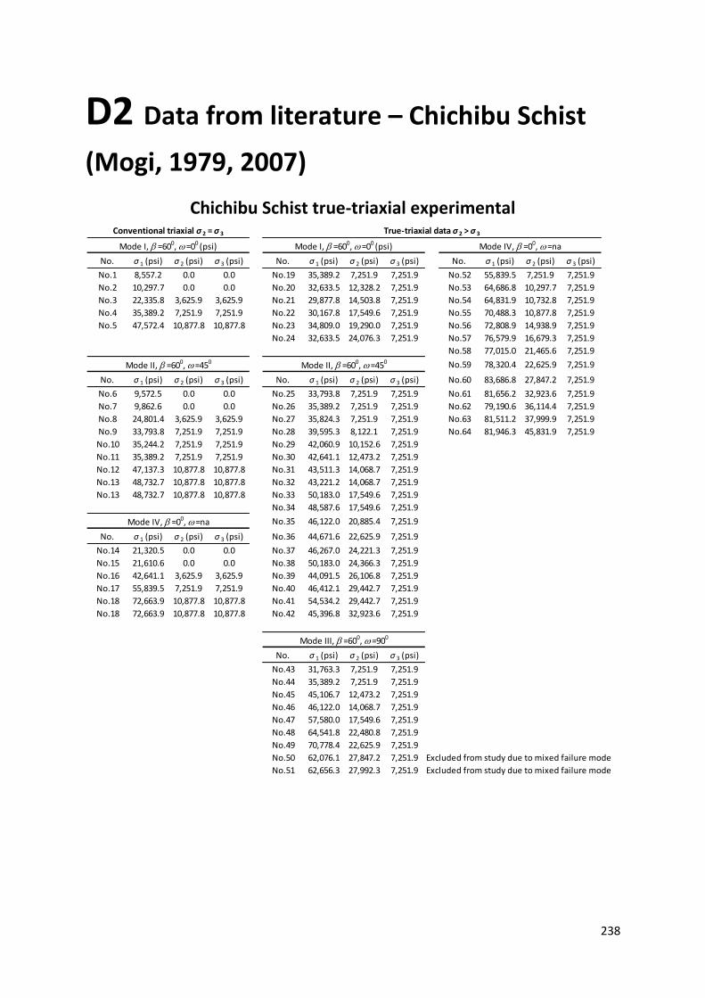
238
D2 Data from literature – Chichibu Schist
(Mogi, 1979, 2007)
Chichibu Schist true-triaxial experimental
No. σ 1 (psi) σ 2 (psi) σ 3 (psi) No. σ 1 (psi) σ 2 (psi) σ 3 (psi) No. σ 1 (psi) σ 2 (psi) σ 3 (psi)
No.1 8,557.2 0.0 0.0 No.19 35,389.2 7,251.9 7,251.9 No.52 55,839.5 7,251.9 7,251.9
No.2 10,297.7 0.0 0.0 No.20 32,633.5 12,328.2 7,251.9 No.53 64,686.8 10,297.7 7,251.9
No.3 22,335.8 3,625.9 3,625.9 No.21 29,877.8 14,503.8 7,251.9 No.54 64,831.9 10,732.8 7,251.9
No.4 35,389.2 7,251.9 7,251.9 No.22 30,167.8 17,549.6 7,251.9 No.55 70,488.3 10,877.8 7,251.9
No.5 47,572.4 10,877.8 10,877.8 No.23 34,809.0 19,290.0 7,251.9 No.56 72,808.9 14,938.9 7,251.9
No.24 32,633.5 24,076.3 7,251.9 No.57 76,579.9 16,679.3 7,251.9
No.58 77,015.0 21,465.6 7,251.9
No.59 78,320.4 22,625.9 7,251.9
No. σ 1 (psi) σ 2 (psi) σ 3 (psi) No. σ 1 (psi) σ 2 (psi) σ 3 (psi) No.60 83,686.8 27,847.2 7,251.9
No.6 9,572.5 0.0 0.0 No.25 33,793.8 7,251.9 7,251.9 No.61 81,656.2 32,923.6 7,251.9
No.7 9,862.6 0.0 0.0 No.26 35,389.2 7,251.9 7,251.9 No.62 79,190.6 36,114.4 7,251.9
No.8 24,801.4 3,625.9 3,625.9 No.27 35,824.3 7,251.9 7,251.9 No.63 81,511.2 37,999.9 7,251.9
No.9 33,793.8 7,251.9 7,251.9 No.28 39,595.3 8,122.1 7,251.9 No.64 81,946.3 45,831.9 7,251.9
No.10 35,244.2 7,251.9 7,251.9 No.29 42,060.9 10,152.6 7,251.9
No.11 35,389.2 7,251.9 7,251.9 No.30 42,641.1 12,473.2 7,251.9
No.12 47,137.3 10,877.8 10,877.8 No.31 43,511.3 14,068.7 7,251.9
No.13 48,732.7 10,877.8 10,877.8 No.32 43,221.2 14,068.7 7,251.9
No.13 48,732.7 10,877.8 10,877.8 No.33 50,183.0 17,549.6 7,251.9
No.34 48,587.6 17,549.6 7,251.9
No.35 46,122.0 20,885.4 7,251.9
No. σ 1 (psi) σ 2 (psi) σ 3 (psi) No.36 44,671.6 22,625.9 7,251.9
No.14 21,320.5 0.0 0.0 No.37 46,267.0 24,221.3 7,251.9
No.15 21,610.6 0.0 0.0 No.38 50,183.0 24,366.3 7,251.9
No.16 42,641.1 3,625.9 3,625.9 No.39 44,091.5 26,106.8 7,251.9
No.17 55,839.5 7,251.9 7,251.9 No.40 46,412.1 29,442.7 7,251.9
No.18 72,663.9 10,877.8 10,877.8 No.41 54,534.2 29,442.7 7,251.9
No.18 72,663.9 10,877.8 10,877.8 No.42 45,396.8 32,923.6 7,251.9
No. σ 1 (psi) σ 2 (psi) σ 3 (psi)
No.43 31,763.3 7,251.9 7,251.9
No.44 35,389.2 7,251.9 7,251.9
No.45 45,106.7 12,473.2 7,251.9
No.46 46,122.0 14,068.7 7,251.9
No.47 57,580.0 17,549.6 7,251.9
No.48 64,541.8 22,480.8 7,251.9
No.49 70,778.4 22,625.9 7,251.9
No.50 62,076.1 27,847.2 7,251.9 Excluded from study due to mixed failure mode
No.51 62,656.3 27,992.3 7,251.9 Excluded from study due to mixed failure mode
True-triaxial data σ 2 > σ 3Conventional triaxial σ 2 = σ 3
Mode IV, =00, =naMode I, =600, =00 (psi)
Mode II, =600, =450
Mode III, =600, =900
Mode I, =600, =00 (psi)
Mode II, =600, =450
Mode IV, =00, =na

239
E JPW model analysis for various
anisotropic rocks
Figure E.1. Plot of the 1 actual / 1 predicted for JPW model
0.00
0.20
0.40
0.60
0.80
1.00
1.20
1.40
1.60
1.80
2.00
0 10 20 30 40 50 60 70 80 90
1
actu
al /
pre
dic
ted
angle
Jaeger Plane of Weakness
1 ratio (actual / predicted) vs
Bossier shale
Vaca Muerta
Angers Schist
Martinsberg Slate
Austin Slate
GRS-1
GRS-2
QuartzPhyllite
CarbonaPhyllite
MicaceousPhyllite
Penrhyn Slate
TournemireShale
0.8 to 1.2 ratio

240
Angle
βσ1
Actualσ3
σ1
Predict(Actual - Predicted)2 Ratio
(Actual/Predicted)
90 6,140 0 12,732 43,460,705 0.482
60 1,811 0 6,372 20,805,340 0.284
45 6,874 0 7,390 266,703 0.930
45 5,653 0 7,390 3,018,672 0.765
30 6,577 0 12,732 37,889,853 0.517
0 16,466 0 12,732 13,939,221 1.293
βσ1
Actualσ3
σ1
Predict(Actual - Predicted)2 Dev in
Ratio
90 21,371 1,000 15,615 33,136,907 1.369
60 6,672 1,000 8,756 4,344,100 0.762
45 8,021 1,000 9,996 3,898,736 0.802
30 13,321 1,000 15,615 5,260,296 0.853
0 18,106 1,000 15,615 6,207,406 1.160
βσ1
Actualσ3
σ1
Predict(Actual - Predicted)2 Dev in
Ratio
90 28,988 3,000 21,379 57,902,153 1.356
75 19,834 3,000 18,377 2,122,188 1.079
60 13,751 3,000 13,524 51,449 1.017
45 15,678 3,000 15,206 223,068 1.031
30 19,367 3,000 21,379 4,046,750 0.906
30 17,500 3,000 21,379 15,043,954 0.819
15 17,103 3,000 21,379 18,281,214 0.800
15 20,956 3,000 21,379 178,636 0.980
0 30,060 3,000 21,379 75,365,775 1.406
βσ1
Actualσ3
σ1
Predict(Actual - Predicted)2 Dev in
Ratio
90 37,437 6,000 30,025 54,940,208 1.247
60 20,330 6,000 20,676 119,763 0.983
45 22,722 6,000 23,021 89,381 0.987
30 25,984 6,000 30,025 16,328,338 0.865
30 24,026 6,000 30,025 35,986,007 0.800
30 23,468 6,000 30,025 42,992,069 0.782
20 30,920 6,000 30,025 801,323 1.030
0 36,951 6,000 30,025 47,971,778 1.231
βσ1
Actualσ3
σ1
Predict(Actual - Predicted)2 Dev in
Ratio
90 47,097 10,000 41,553 30,735,115 1.133
75 39,812 10,000 39,532 78,225 1.007
60 33,197 10,000 30,212 8,910,695 1.099
45 32,556 10,000 33,441 783,797 0.974
30 36,198 10,000 41,553 28,676,818 0.871
15 42,278 10,000 41,553 525,518 1.017
10 38,263 10,000 41,553 10,824,587 0.921
0 42,614 10,000 41,553 1,125,564 1.026
MSE==> 4,171 0.961
Units in psi
0 10 20 30 40 50 60 70 80 900
0.5
1
1.5
2
2.5
3
3.5
4
4.5
5x 10
4
βmin, 57.0
0
5,000
10,000
15,000
20,000
25,000
30,000
35,000
40,000
45,000
50,000
0 10 20 30 40 50 60 70 80 90
σ 1 (
psi)
angle
Jaeger Plane of Weakness - Bossier shale
σ3= 0
σ3= 1,000
σ3= 3,000
σ3= 6,000
σ3= 10,000
JPW σ3 = 0
JPW σ3 = 1,000
JPW σ3 = 3,000
JPW σ3 = 6,000
JPW σ3 = 10,000
βmin
o = 29.0 degSo = 3750 psi
w = 24.0 degSw = 2050 psi

241
Angle
σ3 βσ1
Actual
σ1
Predict(Actual - Predicted)2 Ratio
(Actual/Predicted)
0 60 7,874 8,519 415,109 0.924
0 0 13,730 15,829 4,406,365 0.867
σ3 βσ1
Actual
σ1
Predict(Actual - Predicted)2 Ratio
(Actual/Predicted)
1,000 90 19,075 18,492 340,004 1.032
1,000 60 12,335 11,087 1,558,522 1.113
1,000 0 20,120 18,492 2,650,705 1.088
σ3 βσ1
Actual
σ1
Predict(Actual - Predicted)2 Ratio
(Actual/Predicted)
2,500 90 21,845 22,486 411,280 0.971
2,500 75 19,935 20,304 136,235 0.982
2,500 50 17,010 15,802 1,459,384 1.076
2,500 40 18,005 21,266 10,632,787 0.847
2,500 30 20,535 22,486 3,807,615 0.913
2,500 20 21,950 22,486 287,630 0.976
2,500 15 20,105 22,486 5,670,643 0.894
σ3 βσ1
Actual
σ1
Predict(Actual - Predicted)2 Ratio
(Actual/Predicted)
5,000 90 27,675 29,144 2,156,965 0.950
5,000 80 33,640 29,144 20,217,064 1.154
5,000 60 23,915 21,358 6,537,861 1.120
5,000 40 29,355 29,679 105,240 0.989
5,000 10 30,630 29,144 2,209,204 1.051
5,000 0 30,745 29,144 2,564,287 1.055
σ3 βσ1
Actual
σ1
Predict(Actual - Predicted)2 Ratio
(Actual/Predicted)
20,000 90 67,000 69,088 4,358,742 0.970
20,000 60 61,000 59,876 1,263,062 1.019
20,000 0 69,965 69,088 769,550 1.013
MSE ==> 1,851 1.000
Units in psi
0 10 20 30 40 50 60 70 80 900
1
2
3
4
5
6
7
8x 10
4
βmin, 58.0
0
10,000
20,000
30,000
40,000
50,000
60,000
70,000
80,000
0 10 20 30 40 50 60 70 80 90
σ1
(p
si)
angle
Jaeger Plane of Weakness - Vaca Muerta
σ3= 0
σ3= 1,000
σ3= 2,500
σ3= 5,000
σ3= 20,000
JPW σ3 = 0
JPW σ3 = 1,000
JPW σ3 = 2,500
JPW σ3 = 5,000
JPW σ3 = 20,000
βmin
o = 27.0 degSo = 4850.0 psi
w = 26.0 degSw = 2650.0 psi

242
β1
Actual3
1
Predicted(Actual - Predicted)2 Dev in
Ratio
0 21,509 0 22,927 2,009,538 0.938
15 10,182 0 13,847 13,432,777 0.735
30 5,279 0 4,924 126,257 1.072
45 1,537 0 3,739 4,846,006 0.411
60 1,755 0 4,030 5,177,450 0.435
75 3,713 0 6,657 8,667,590 0.558
90 14,098 0 22,927 77,951,388 0.615
β1
Actual3
1
Predicted(Actual - Predicted)2 Dev in
Ratio
0 35,302 725 26,451 78,344,747 1.335
15 13,866 725 15,476 2,594,294 0.896
30 5,482 725 5,971 238,549 0.918
45 3,321 725 4,708 1,923,160 0.705
60 3,466 725 5,019 2,409,885 0.691
75 8,122 725 7,817 93,078 1.039
90 27,485 725 26,451 1,068,587 1.039
β1
Actual3
1
Predicted(Actual - Predicted)2 Dev in
Ratio
0 34,824 1,450 29,975 23,506,844 1.162
15 21,296 1,450 17,106 17,556,409 1.245
30 5,860 1,450 7,018 1,341,221 0.835
45 3,814 1,450 5,678 3,470,887 0.672
60 4,873 1,450 6,007 1,285,818 0.811
75 9,645 1,450 8,977 446,226 1.074
90 26,846 1,450 29,975 9,788,687 0.896
β1
Actual3
1
Predicted(Actual - Predicted)2 Dev in
Ratio
0 39,784 2,901 37,024 7,618,604 1.075
15 22,930 2,901 20,365 6,581,713 1.126
30 6,179 2,901 9,111 8,600,238 0.678
45 8,121 2,901 7,616 254,398 1.066
60 7,919 2,901 7,984 4,225 0.992
75 13,895 2,901 11,297 6,747,745 1.230
90 34,824 2,901 37,024 4,840,473 0.941
β1
Actual3
1
Predicted(Actual - Predicted)2 Dev in
Ratio
0 49,371 4,351 44,072 28,076,015 1.120
15 20,363 4,351 23,624 10,632,877 0.862
30 12,662 4,351 11,205 2,122,793 1.130
45 8,760 4,351 9,555 631,650 0.917
60 10,602 4,351 9,961 411,333 1.064
75 17,550 4,351 13,617 15,465,568 1.289
90 39,262 4,351 44,072 23,140,402 0.891
β1
Actual3
1
Predicted(Actual - Predicted)2 Dev in
Ratio
0 51,430 5,802 51,121 95,928 1.006
15 27,195 5,802 26,883 96,932 1.012
30 14,112 5,802 13,298 662,221 1.061
45 11,908 5,802 11,494 171,226 1.036
60 12,763 5,802 11,938 681,558 1.069
75 20,247 5,802 15,937 18,579,258 1.270
90 48,863 5,802 51,121 5,096,057 0.956
MSE==> 3,074 0.949
βmin, 49.1
0
10,000
20,000
30,000
40,000
50,000
0 10 20 30 40 50 60 70 80 90
σ1
(p
si)
angle
Jaeger Plane of weakness - Angers Schist (Duveau, 1998)
σ3= 0 psi
σ3= 725 psi
σ3= 1,450 psi
σ3= 2,901 psi
σ3= 4,351 psi
σ3= 5,802 psi
JPW σ3 = 0
JPW σ3 = 725
JPW σ3 = 1,450
JPW σ3 = 2,901
JPW σ3 = 4,351
JPW σ3 = 5,802
βmin
o = 41.2degSo = 5200.0 psi
w = 8.2degSw = 1600.0 psi
0 10 20 30 40 50 60 70 80 900
0.5
1
1.5
2
2.5
3
3.5
4
4.5
5
5.5x 10
4

243
Angle
βσ1
Actualσ3
σ1
Predict(Actual - Predicted)2 Dev in
Ratio
90 19,245 508 26,286 49,574,202 0.732
75 7,551 508 9,444 3,583,173 0.800
60 3,176 508 6,250 9,450,490 0.508
45 5,733 508 6,390 431,482 0.897
30 10,869 508 10,447 178,010 1.040
15 18,176 508 26,286 65,769,231 0.691
0 28,478 508 26,286 4,805,773 1.083
βσ1
Actualσ3
σ1
Predict(Actual - Predicted)2 Dev in
Ratio
90 24,200 1,523 29,369 26,721,748 0.824
75 11,954 1,523 11,793 25,962 1.014
60 6,634 1,523 8,123 2,217,317 0.817
45 9,194 1,523 8,284 828,587 1.110
30 14,598 1,523 12,946 2,728,156 1.128
15 23,131 1,523 29,369 38,915,593 0.788
0 35,060 1,523 29,369 32,388,819 1.194
βσ1
Actualσ3
σ1
Predict(Actual - Predicted)2 Dev in
Ratio
90 38,479 5,076 40,159 2,824,085 0.958
75 18,768 5,076 20,015 1,556,293 0.938
60 12,227 5,076 14,677 6,005,015 0.833
45 15,190 5,076 14,911 77,852 1.019
30 21,277 5,076 21,693 173,235 0.981
15 31026 5,076 40,159 83,403,294 0.773
0 48,798 5,076 40,159 74,631,175 1.215
βσ1
Actualσ3
σ1
Predict(Actual - Predicted)2 Dev in
Ratio
90 51,517 7,252 46,765 22,583,137 1.102
75 26237 7,252 25,050 1,410,714 1.047
60 18,473 7,252 18,690 46,852 0.988
45 21,170 7,252 18,968 4,846,652 1.116
30 27,795 7,252 27,049 557,301 1.028
15 40,262 7,252 46,765 42,285,844 0.861
0 60,070 7,252 46,765 177,024,281 1.285
βσ1
Actualσ3
σ1
Predict(Actual - Predicted)2 Dev in
Ratio
90 77,775 14,504 68,786 80,803,422 1.131
75 42,859 14,504 41,830 1,057,636 1.025
60 33,465 14,504 32,066 1,956,998 1.044
45 36,974 14,504 32,493 20,084,395 1.138
30 46,318 14,504 44,899 2,011,991 1.032
15 64,485 14,504 68,786 18,496,326 0.937
0 87,954 14,504 68,786 367,405,356 1.279
βσ1
Actualσ3
σ1
Predict(Actual - Predicted)2 Dev in
Ratio
90 108,159 29,008 112,827 21,794,284 0.959
75 72,841 29,008 75,392 6,505,944 0.966
60 60,732 29,008 58,817 3,665,630 1.033
45 63,560 29,008 59,542 16,140,750 1.067
30 77,249 29,008 80,601 11,239,280 0.958
15 96774 29,008 112,827 257,727,620 0.858
0 119,154 29,008 112,827 40,029,360 1.056
MSE==> 5,984 0.982
Units in psi
βmin, 53.4
0
20,000
40,000
60,000
80,000
100,000
120,000
0 10 20 30 40 50 60 70 80 90
σ1
(p
si)
angle
Jaeger Plane of weakness - Martinsburg Slate (Donath 1964)
σ3= 508 psi
σ3= 1,523 psi
σ3= 5,076 psi
σ3= 7,252 psi
σ3= 14,504 psi
σ3= 29,008 psi
JPW σ3 = 508
JPW σ3 = 1,523
JPW σ3 = 5,076
JPW σ3 = 7,252
JPW σ3 = 14,504
JPW σ3 = 29,008
βmin
o = 30.3degSo = 7100.psi
w = 16.8degSw = 1900.0 psi

244
Angle
βσ1
Actualσ3
σ1
Predict(Actual - Predicted)2 Ratio
(Actual/Predicted)
90 50,244 5,000 46,045 17,629,539 1.091
80 39,361 5,000 46,045 44,679,139 0.855
70 25,072 5,000 31,475 40,991,812 0.797
60 21,649 5,000 25,829 17,480,443 0.838
50 24,388 5,000 24,772 148,122 0.984
40 28,262 5,000 27,143 1,251,784 1.041
30 32,622 5,000 35,845 10,389,500 0.910
20 38,280 5,000 46,045 60,295,933 0.831
10 44,585 5,000 46,045 2,130,273 0.968
0 47,649 5,000 46,045 2,574,274 1.035
βσ1
Actualσ3
σ1
Predict(Actual - Predicted)2 Ratio
(Actual/Predicted)
90 68,865 10,000 57,118 137,989,618 1.206
80 54,090 10,000 57,118 9,168,189 0.947
70 37,856 10,000 40,602 7,541,521 0.932
60 31,351 10,000 34,077 7,428,952 0.920
50 34,252 10,000 32,855 1,952,888 1.043
40 36,505 10,000 35,595 828,019 1.026
30 43,135 10,000 45,653 6,342,411 0.945
20 48,955 10,000 57,118 66,626,435 0.857
10 52,504 10,000 57,118 21,283,476 0.919
0 60,271 10,000 57,118 9,939,506 1.055
βσ1
Actualσ3
σ1
Predict(Actual - Predicted)2 Ratio
(Actual/Predicted)
90 95,243 20,000 79,264 255,331,184 1.202
80 77,873 20,000 79,264 1,933,808 0.982
70 60,180 20,000 58,856 1,751,972 1.022
60 53,351 20,000 50,571 7,731,139 1.055
50 53,333 20,000 49,019 18,607,189 1.088
40 53,477 20,000 52,498 959,034 1.019
30 63,513 20,000 65,270 3,087,378 0.973
20 73,063 20,000 79,264 38,450,096 0.922
10 78,558 20,000 79,264 497,891 0.991
0 85,513 20,000 79,264 39,051,074 1.079
βσ1
Actualσ3
σ1
Predict(Actual - Predicted)2 Ratio
(Actual/Predicted)
90 120,973 30,000 101,410 382,706,016 1.193
80 98,090 30,000 101,410 11,024,569 0.967
70 83,477 30,000 77,110 40,537,725 1.083
60 71,297 30,000 67,065 17,912,327 1.063
50 68,685 30,000 65,184 12,254,569 1.054
40 71,261 30,000 69,402 3,458,672 1.027
30 83,244 30,000 84,887 2,699,360 0.981
20 92,144 30,000 101,410 85,851,836 0.909
10 100,883 30,000 101,410 277,862 0.995
0 105,567 30,000 101,410 17,280,428 1.041
βσ1
Actualσ3
σ1
Predict(Actual - Predicted)2 Ratio
(Actual/Predicted)
90 136,000 40,000 123,556 154,839,722 1.101
80 112,143 40,000 123,556 130,250,611 0.908
70 99,315 40,000 95,365 15,606,671 1.041
60 86,486 40,000 83,559 8,569,664 1.035
50 84,522 40,000 81,348 10,071,738 1.039
40 86,289 40,000 86,305 272 1.000
30 97,622 40,000 104,503 47,359,891 0.934
20 108,630 40,000 123,556 222,783,655 0.879
0 124,162 40,000 123,556 366,825 1.005
MSE==> 6,385.5 1.007
Units in psi
βmin, 51.8
0
20,000
40,000
60,000
80,000
100,000
120,000
140,000
0 10 20 30 40 50 60 70 80 90
σ1
(p
si)
β= 00 to 900
Jaeger Plane of weakness - Austin Slate(McLamore & Gray1967)
σ3= 5,000 psi
σ3= 10,000 psi
σ3= 20,000 psi
σ3= 30,000 psi
σ3= 40,000 psi
JPW σ3 = 5,000
JPW σ3 = 10,000
JPW σ3 = 20,000
JPW σ3 = 30,000
JPW σ3 = 40,000
βmin
o = 22.2degSo = 11,750.0 psi
w = 13.6degSw = 6550.0 psi

245
Angle
βσ1
Actualσ3
σ1
Predict(Actual - Predicted)2 Dev in
Ratio
90 36,553 1,000 35,239 1,725,483 1.037
75 30,060 1,000 32,771 7,349,399 0.917
70 28,165 1,000 27,492 452,847 1.024
60 23,207 1,000 24,409 1,445,075 0.951
45 31,649 1,000 33,554 3,626,979 0.943
30 32,174 1,000 35,239 9,396,208 0.913
15 31,439 1,000 35,239 14,442,458 0.892
0 33,224 1,000 35,239 4,063,544 0.943
βσ1
Actualσ3
σ1
Predict(Actual - Predicted)2 Dev in
Ratio
90 50,090 5,000 46,231 14,889,938 1.083
75 46,566 5,000 46,231 111,922 1.007
70 42,692 5,000 40,824 3,489,099 1.046
60 37,733 5,000 36,654 1,164,520 1.029
45 43,387 5,000 46,231 8,090,906 0.938
30 44,092 5,000 46,231 4,577,682 0.954
15 44,347 5,000 46,231 3,553,043 0.959
0 46,671 5,000 46,231 193,203 1.010
βσ1
Actualσ3
σ1
Predict(Actual - Predicted)2 Dev in
Ratio
90 63,638 10,000 59,972 13,441,666 1.061
75 61,103 10,000 59,972 1,280,943 1.019
70 58,399 10,000 57,489 828,336 1.016
60 53,710 10,000 51,961 3,059,638 1.034
45 58,824 10,000 59,972 1,317,014 0.981
30 61,328 10,000 59,972 1,840,059 1.023
15 60,953 10,000 59,972 963,711 1.016
0 61,928 10,000 59,972 3,826,670 1.033
βσ1
Actualσ3
σ1
Predict(Actual - Predicted)2 Dev in
Ratio
90 78,085 15,000 73,712 19,125,116 1.059
75 75,191 15,000 73,712 2,188,113 1.020
70 72,936 15,000 73,712 601,203 0.989
60 68,338 15,000 67,268 1,144,547 1.016
45 74,891 15,000 73,712 1,391,049 1.016
30 74,336 15,000 73,712 389,784 1.008
15 75,311 15,000 73,712 2,556,888 1.022
0 76,645 15,000 73,712 8,604,995 1.040
βσ1
Actualσ3
σ1
Predict(Actual - Predicted)2 Dev in
Ratio
90 103,921 25,000 101,192 7,444,201 1.027
75 99,137 25,000 101,192 4,223,410 0.980
70 98,232 25,000 101,192 8,760,379 0.971
60 96,333 25,000 97,882 2,398,965 0.984
45 96,768 25,000 101,192 19,576,145 0.956
30 99,362 25,000 101,192 3,350,341 0.982
15 100,516 25,000 101,192 456,697 0.993
0 100,591 25,000 101,192 360,953 0.994
MSE==> 2,166 0.997
Units in psi
βmin, 60.3
0
20,000
40,000
60,000
80,000
100,000
0 10 20 30 40 50 60 70 80 90
σ1
(p
si)
angle
Jaeger Plane of weakness - GreenRiver1 (McLamore & Gray1967)
σ3= 1,000 psi
σ3= 5,000 psi
σ3= 10,000 psi
σ3= 15,000 psi
σ3= 25,000 psi
JPW σ3 = 1,000
JPW σ3 = 5,000
JPW σ3 = 10,000
JPW σ3 = 15,000
JPW σ3 = 25,000
βmin
o = 27.8 degSo = 9800.0 psi
w = 30.5 degSw = 6100.0 psi

246
Angle
βσ1
Actualσ3
σ1
Predict(Actual - Predicted)2 Dev in
Ratio
90 21,556 1,000 19,851 2,906,787 1.086
80 19,227 1,000 19,851 389,089 0.969
70 16,292 1,000 16,396 10,787 0.994
60 13,559 1,000 13,453 11,287 1.008
50 14,715 1,000 13,306 1,984,861 1.106
30 17,380 1,000 19,851 6,102,233 0.876
0 18677 1,000 19,851 1,377,970 0.941
βσ1
Actualσ3
σ1
Predict(Actual - Predicted)2 Dev in
Ratio
90 29,445 5,000 27,771 2,801,257 1.060
80 27,368 5,000 27,771 162,010 0.986
70 24,635 5,000 25,200 319,040 0.978
60 21,499 5,000 21,339 25,419 1.007
50 22,756 5,000 21,146 2,589,492 1.076
30 25,724 5,000 27,771 4,189,818 0.926
0 27273 5,000 27,771 248,108 0.982
βσ1
Actualσ3
σ1
Predict(Actual - Predicted)2 Dev in
Ratio
90 40,960 10,000 37,671 10,815,726 1.087
80 38,479 10,000 37,671 653,393 1.021
70 34,736 10,000 36,206 2,159,897 0.959
60 30,640 10,000 31,197 310,169 0.982
50 32,958 10,000 30,947 4,043,068 1.065
30 36,633 10,000 37,671 1,078,011 0.972
0 38081 10,000 37,671 167,958 1.011
βσ1
Actualσ3
σ1
Predict(Actual - Predicted)2 Dev in
Ratio
90 51,667 15,000 47,571 16,771,963 1.086
80 48,782 15,000 47,571 1,467,148 1.025
70 45,393 15,000 47,212 3,307,237 0.961
60 40,438 15,000 41,055 380,305 0.985
50 42,958 15,000 40,747 4,885,367 1.054
30 46,532 15,000 47,571 1,080,023 0.978
0 47929 15,000 47,571 128,278 1.008
βσ1
Actualσ3
σ1
Predict(Actual - Predicted)2 Dev in
Ratio
90 71,515 25,000 67,371 17,169,602 1.062
80 66,560 25,000 67,371 658,172 0.988
70 64,181 25,000 67,371 10,179,789 0.953
60 58,620 25,000 60,770 4,625,120 0.965
50 61,442 25,000 60,348 1,196,800 1.018
30 64,108 25,000 67,371 10,652,248 0.952
0 67,374 25,000 67,371 5 1.000
MSE==> 1,811 1.004
Units in psi
βmin, 54.4
0
10,000
20,000
30,000
40,000
50,000
60,000
70,000
80,000
0 10 20 30 40 50 60 70 80 90
σ1
(p
si)
angle
Jaeger Plane of Weakness - GreenRiver2 (McLamore & Gray1967)
σ3= 1,000 psi
σ3= 5,000 psi
σ3= 10,000 psi
σ3= 15,000 psi
σ3= 25,000 psi
JPW σ3 = 1,000
JPW σ3 = 5,000
JPW σ3 = 10,000
JPW σ3 = 15,000
JPW σ3 = 25,000
βmin
o = 19.2 degSo = 6350.0 psi
w = 18.7 degSw = 4000.0 psi

247
Angle
βσ1
Actualσ3
σ1
Predict(Actual - Predicted)2 Dev in
Ratio
90 9,512 0 12,551 9,233,508 0.758
65 6,795 0 7,594 638,741 0.895
55 6,585 0 7,256 449,289 0.908
30 8,624 0 12,551 15,422,776 0.687
0 14,739 0 12,551 4,787,203 1.174
βσ1
Actualσ3
σ1
Predict(Actual - Predicted)2 Dev in
Ratio
90 12,119 725 14,951 8,016,621 0.811
60 8,356 725 9,076 517,751 0.921
30 9,715 725 14,951 27,411,463 0.650
25 14,262 725 14,951 473,998 0.954
0 18,077 725 14,951 9,778,053 1.209
βσ1
Actualσ3
σ1
Predict(Actual - Predicted)2 Dev in
Ratio
90 20,364 2,176 19,749 377,723 1.031
60 14,719 2,176 12,786 3,738,131 1.151
30 18,117 2,176 19,749 2,665,929 0.917
20 20,730 2,176 19,749 961,424 1.050
0 25,382 2,176 19,749 31,721,353 1.285
βσ1
Actualσ3
σ1
Predict(Actual - Predicted)2 Dev in
Ratio
90 28,550 4,351 26,948 2,567,805 1.059
50 19,822 4,351 19,304 268,538 1.027
40 23,742 4,351 25,381 2,686,871 0.935
30 25,623 4,351 26,948 1,754,098 0.951
20 29,073 4,351 26,948 4,515,659 1.079
0 32,627 4,351 26,948 32,252,821 1.211
βσ1
Actualσ3
σ1
Predict(Actual - Predicted)2 Dev in
Ratio
90 39,709 7,252 36,546 10,006,923 1.087
85 36,155 7,252 36,546 152,706 0.989
60 27,008 7,252 25,772 1,527,726 1.048
30 34,064 7,252 36,546 6,157,098 0.932
20 38,716 7,252 36,546 4,710,198 1.059
0 39,709 7,252 36,546 10,006,923 1.087
βσ1
Actualσ3
σ1
Predict(Actual - Predicted)2 Dev in
Ratio
90 47,418 10,153 46,143 1,624,938 1.028
80 42,192 10,153 46,143 15,617,103 0.914
50 35,345 10,153 34,760 341,977 1.017
30 40,415 10,153 46,143 32,819,721 0.876
15 45,328 10,153 46,143 665,600 0.982
0 47,732 10,153 46,143 2,522,703 1.034
MSE==> 2,692 0.991
Units in psi
βmin, 58.0
0
5,000
10,000
15,000
20,000
25,000
30,000
35,000
40,000
45,000
50,000
0 10 20 30 40 50 60 70 80 90
σ1
(p
si)
angle
Jaeger Plane of weakness - Quartz Phyllite (Ramamurthy, 1993)σ3= 0 psi
σ3= 725 psi
σ3= 2,176 psi
σ3= 4,351 psi
σ3= 7,252 psi
σ3= 10,153 psi
JPW σ3 = 0
JPW σ3 = 725
JPW σ3 = 2,176
JPW σ3 = 4,351
JPW σ3 = 7,252
JPW σ3 = 10,153
βmin
o = 36.6degSo = 3122.3psi
w = 27.8degSw = 1532.1 psi

248
Angle
βσ1
Actualσ3
σ1
Predict(Actual - Predicted)2 Dev in
Ratio
90 9,446 0 11,738 5,255,566 0.805
65 5,584 0 6,311 527,748 0.885
60 5,427 0 6,078 423,374 0.893
30 7,045 0 11,738 22,025,399 0.600
0 11,533 0 11,738 42,026 0.983
βσ1
Actualσ3
σ1
Predict(Actual - Predicted)2 Dev in
Ratio
90 12,415 725 14,178 3,107,478 0.876
85 14,764 725 14,178 342,965 1.041
65 8,762 725 8,428 111,847 1.040
30 11,267 725 14,178 8,473,470 0.795
0 16,747 725 14,178 6,598,684 1.181
βσ1
Actualσ3
σ1
Predict(Actual - Predicted)2 Dev in
Ratio
90 20,650 2,176 19,057 2,536,965 1.084
60 14,022 2,176 12,276 3,049,821 1.142
35 14,857 2,176 19,057 17,639,805 0.780
30 18,510 2,176 19,057 299,002 0.971
0 25,921 2,176 19,057 47,111,002 1.360
βσ1
Actualσ3
σ1
Predict(Actual - Predicted)2 Dev in
Ratio
90 25,852 4,351 26,376 273,931 0.980
90 29,088 4,351 26,376 7,356,365 1.103
80 28,462 4,351 26,376 4,351,351 1.079
55 20,112 4,351 18,786 1,758,051 1.071
25 27,001 4,351 26,376 390,293 1.024
10 28,931 4,351 26,376 6,531,200 1.097
0 30,080 4,351 26,376 13,717,688 1.140
βσ1
Actualσ3
σ1
Predict(Actual - Predicted)2 Dev in
Ratio
90 36,216 7,252 36,134 6,709 1.002
60 29,275 7,252 26,737 6,442,488 1.095
50 27,240 7,252 28,929 2,852,741 0.942
30 33,711 7,252 36,134 5,871,101 0.933
25 32,980 7,252 36,134 9,946,047 0.913
0 39,556 7,252 36,134 11,709,974 1.095
βσ1
Actualσ3
σ1
Predict(Actual - Predicted)2 Dev in
Ratio
90 46,423 10,153 45,892 281,653 1.012
75 41,256 10,153 44,646 11,492,288 0.924
55 37,447 10,153 35,550 3,596,953 1.053
30 39,847 10,153 45,892 36,540,386 0.868
5 46,893 10,153 45,892 1,000,684 1.022
MSE==> 2,706 0.994
Units in psi
βmin, 59.4
0
5,000
10,000
15,000
20,000
25,000
30,000
35,000
40,000
45,000
50,000
0 10 20 30 40 50 60 70 80 90
σ1
(p
si)
angle
Jaeger Plane of Weakness - Carbona Phyllite (Ramamurthy et al., 1993) σ3= 0 psi
σ3= 725 psi
σ3= 2,176 psi
σ3= 4,351 psi
σ3= 7,252 psi
σ3= 10,153 psi
JPW σ3 = 0
JPW σ3 = 725
JPW σ3 = 2,176
JPW σ3 = 4,351
JPW σ3 = 7,252
JPW σ3 = 10,153
βmin
o = 32.8 degSo = 3200.0 psi
w = 28.7 degSw = 1800.0 psi

249
Angle
βσ1
Actualσ3
σ1
Predict(Actual - Predicted)2 Dev in
Ratio
90 9,800 0 13,562 14,150,978 0.723
75 4981.9145 0 6,704 2,965,481 0.743
60 2,473 0 4,477 4,018,333 0.552
0 14,211 0 13,562 420,475 1.048
βσ1
Actualσ3 (Actual - Predicted)2 Dev in
Ratio
90 16615.954 725 16,284 109,901 1.020
75 9,277 725 8,699 334,224 1.066
60 4,529 725 6,051 2,315,986 0.748
20 9,109 725 16,284 51,483,756 0.559
0 17,946 725 16,284 2,761,092 1.102
βσ1
Actualσ3
σ1
Predict(Actual - Predicted)2 Dev in
Ratio
90 25,417 2,176 21,729 13,599,355 1.170
75 16,257 2,176 12,690 12,725,608 1.281
10 20,088 2,176 21,729 2,691,781 0.924
0 22,967 2,176 21,729 1,532,034 1.057
βσ1
Actual σ3σ1
Predict (Actual - Predicted)2 Dev in
Ratio
90 32,282 4,351 29,895 5,698,248 1.080
75 21,582 4,351 18,676 8,445,179 1.156
60 15,573 4,351 13,918 2,740,280 1.119
10 28,916 4,351 29,895 958,881 0.967
0 31,652 4,351 29,895 3,087,248 1.059
βσ1
Actualσ3
σ1
Predict(Actual - Predicted)2 Dev in
Ratio
90 51,704 7,252 40,784 119,241,136 1.268
75 19,946 7,252 26,658 45,049,978 0.748
0 39,313 7,252 40,784 2,163,714 0.964
βσ1
Actualσ3
σ1
Predict(Actual - Predicted)2 Dev in
Ratio
90 63985.122 10152.639 51,673 151,590,555 1.238
75 37,047 10,153 34,639 5,796,920 1.070
60 26,694 10,153 26,505 35,788 1.007
20 36,528 10,153 51,673 229,376,036 0.707
0 46,134 10,153 51,673 30,677,623 0.893
MSE ==> 5,240 0.972
Units in psi
βmin, 55.7
0
10,000
20,000
30,000
40,000
50,000
60,000
70,000
0 10 20 30 40 50 60 70 80 90
σ1
(p
si)
angle
Jaeger Plane of weakness - Micaceous Phyllite (Ramamurthy, 1993)σ3= 0 psi
σ3= 725 psi
σ3= 2,176 psi
σ3= 4,351 psi
σ3= 7,252 psi
σ3= 10,153 psi
JPOW σ3 = 0
JPOW σ3 = 725
JPOW σ3 = 2,176
JPOW σ3 = 4,351
JPOW σ3 = 7,252
JPOW σ3 = 10,153
βmin
o = 35.4degSo = 3500.0 psi
w = 21.4 degSw = 1500.0 psi

250
Angle
βσ1
Actualσ3
σ1
Predict(Actual - Predicted)2 Dev in
Ratio
90 27,167 0 26,990 31,595 1.007
75 16,432 0 21,383 24,514,683 0.768
60 6,354 0 13,527 51,449,597 0.470
45 9,092 0 13,475 19,208,985 0.675
30 12,488 0 21,037 73,074,990 0.594
15 18,404 0 26,990 73,716,802 0.682
0 30,235 0 26,990 10,530,357 1.120
βσ1
Actualσ3
σ1
Predict(Actual - Predicted)2 Dev in
Ratio
90 29,373 1,000 30,696 1,750,566 0.957
75 21,485 1,000 23,512 4,107,734 0.914
60 13,379 1,000 15,241 3,466,391 0.878
45 14,803 1,000 15,186 147,172 0.975
30 18,308 1,000 23,147 23,414,259 0.791
15 24,443 1,000 30,696 39,096,125 0.796
0 36,383 1,000 30,696 32,351,189 1.185
βσ1
Actualσ3
σ1
Predict(Actual - Predicted)2 Dev in
Ratio
90 40,013 2,000 34,402 31,482,985 1.163
75 29,496 2,000 25,641 14,865,043 1.150
60 18,542 2,000 16,955 2,518,468 1.094
45 20,404 2,000 16,898 12,292,559 1.207
30 25,443 2,000 25,258 34,349 1.007
15 31,139 2,000 34,402 10,642,144 0.905
0 45,271 2,000 34,402 118,138,858 1.316
βσ1
Actualσ3
σ1
Predict(Actual - Predicted)2 Dev in
Ratio
90 51,462 6,000 49,225 5,001,521 1.045
75 37,002 6,000 34,155 8,100,424 1.083
60 29,662 6,000 23,811 34,239,348 1.246
60 23,856 6,000 23,811 2,065 1.002
45 25,280 6,000 23,743 2,362,968 1.065
30 32,510 6,000 33,699 1,413,992 0.965
15 37,440 6,000 49,225 138,900,178 0.761
0 52,557 6,000 49,225 11,100,945 1.068
βσ1
Actualσ3
σ1
Predict(Actual - Predicted)2 Dev in
Ratio
90 55,105 8,000 56,637 2,347,860 0.973
75 41,193 8,000 38,413 7,726,042 1.072
60 27,171 8,000 27,239 4,621 0.998
45 33,415 8,000 27,165 39,052,565 1.230
30 37,139 8,000 37,920 609,786 0.979
15 43,931 8,000 56,637 161,444,291 0.776
0 63,321 8,000 56,637 44,670,870 1.118
βσ1
Actualσ3
σ1
Predict(Actual - Predicted)2 Dev in
Ratio
90 70,908 10,000 64,049 47,041,025 1.107
75 50,203 10,000 42,670 56,746,504 1.177
45 36,948 10,000 30,588 40,453,611 1.208
30 40,125 10,000 42,141 4,063,702 0.952
15 50,751 10,000 64,049 176,832,921 0.792
0 77,919 10,000 64,049 192,364,306 1.217
MSE==> 6,018 0.988
Units in psi
βmin, 52.4
0
10,000
20,000
30,000
40,000
50,000
60,000
70,000
80,000
0 10 20 30 40 50 60 70 80 90
σ1
(p
si)
angle
Jaeger Plane of weakness - Penrhyn Slate (Attenwell & Sandford, 1974)
σ3= 0 psi
σ3= 1,000 psi
σ3= 2,000 psi
σ3= 6,000 psi
σ3= 8,000 psi
σ3= 10,000 psi
JPW σ3 = 0
JPW σ3 = 1,000
JPW σ3 = 2,000
JPW σ3 = 6,000
JPW σ3 = 8,000
JPW σ3 = 10,000
βmin
o = 35.1 degSo = 7010.0 psi
w = 14.7 degSw = 4970.0 psi
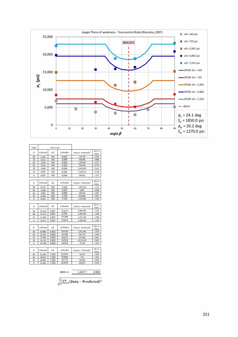
251
Angle
β σ1Actual σ3 σ1Predict (Actual - Predicted)2 Dev in
Ratio
90 5,163 145 6,054 793,720 0.853
70 4,351 145 4,899 300,894 0.888
60 2,926 145 4,026 1,209,987 0.727
45 3,375 145 4,332 916,799 0.779
30 3,699 145 6,054 5,543,874 0.611
15 4,587 145 6,054 2,149,535 0.758
0 6,825 145 6,054 594,851 1.127
β σ1Actual σ3 σ1Predict (Actual - Predicted)2 Dev in
Ratio
90 8,722 725 7,435 1,657,256 1.173
60 5,168 725 5,232 4,087 0.988
45 5,962 725 5,588 140,024 1.067
30 6,506 725 7,435 862,809 0.875
0 8,503 725 7,435 1,140,694 1.144
β σ1Actual σ3 σ1Predict (Actual - Predicted)2 Dev in
Ratio
90 15,256 2,901 12,613 6,987,905 1.210
60 12,173 2,901 9,754 5,847,994 1.248
45 11,305 2,901 10,296 1,017,236 1.098
0 14,911 2,901 12,613 5,283,200 1.182
β σ1Actual σ3 σ1Predict (Actual - Predicted)2 Dev in
Ratio
90 20,886 5,802 19,518 1,871,946 1.070
60 16,391 5,802 15,785 367,179 1.038
45 15,930 5,802 16,574 414,440 0.961
30 15,753 5,802 19,518 14,174,555 0.807
0 19,788 5,802 19,518 73,156 1.014
β σ1Actual σ3 σ1Predict (Actual - Predicted)2 Dev in
Ratio
90 23,183 7,252 22,970 45,376 1.009
60 18,813 7,252 18,800 176 1.001
45 18,855 7,252 19,713 736,642 0.956
0 22,461 7,252 22,970 258,472 0.978
MSE==> 1,447.7 0.982
Units in psi
βmin, 55.1
0
5,000
10,000
15,000
20,000
25,000
0 10 20 30 40 50 60 70 80 90
σ1
(p
si)
angle
Jaeger Plane of weakness - Tournemire Shale (Niandou,1997)σ3= 145 psi
σ3= 725 psi
σ3= 2,901 psi
σ3= 5,802 psi
σ3= 7,252 psi
JPOW σ3 = 145
JPOW σ3 = 725
JPOW σ3 = 2,901
JPOW σ3 = 5,802
JPOW σ3 = 7,252
βmin
o = 24.1 degSo = 1850.0 psi
w = 20.2 degSw = 1270.0 psi

252
F Pariseau model analysis for various
anisotropic rocks
Figure F.1. Plot of the 1 actual / 1 predicted for Pariseau model
0.00
0.20
0.40
0.60
0.80
1.00
1.20
1.40
1.60
1.80
2.00
0 10 20 30 40 50 60 70 80 90
1
actu
al /
pre
dic
ted
Pariseau model
1 ratio (actual / predicted) vs
Bossier shale
Vaca Muerta
Angers Schist
Martinsburg Slate
Austin slate
GRS-1
GRS-2
Quartz Phyllite
Carbona Phyllite
Micaceous Phyllite
Penrhyn slate
Tournemire shale
0.8 to 1.2 ratio

253
3 β1
Actual
1
Predicted(Actual - Predicted)2 Ratio
(Actual/Predicted)
0 90 6,140 15,305 84,001,130 0.401
0 60 1,811 9,073 52,736,672 0.200
0 45 6,874 8,273 1,956,871 0.831
0 45 5,653 8,273 6,863,782 0.683
0 30 6,577 9,262 7,211,607 0.710
0 0 16,466 14,701 3,113,513 1.120
3 β1
Actual
1
Predicted(Actual - Predicted)2 Ratio
(Actual/Predicted)
1,000 90 21,371 18,601 7,672,928 1.149 F = psi-2
1,000 60 6,672 11,434 22,676,189 0.584 G = psi-2
1,000 45 8,021 10,514 6,214,124 0.763 U = psi-1
1,000 30 13,321 11,652 2,786,195 1.143 V = psi-1
1,000 0 18,106 17,907 39,717 1.011 M = psi-2
3 β1
Actual
1
Predicted(Actual - Predicted)2 Ratio
(Actual/Predicted)
3,000 90 28,988 25,193 14,405,373 1.151
3,000 75 19,834 20,556 521,453 0.965
3,000 60 13,751 16,156 5,783,317 0.851
3,000 45 15,678 14,996 465,562 1.046 Mean Error = ==> 3,248 psi
3,000 30 19,367 16,431 8,622,779 1.179
3,000 30 17,500 16,431 1,143,738 1.065
3,000 15 17,103 20,649 12,570,797 0.828
3,000 15 20,956 20,649 94,537 1.015
3,000 0 30,060 24,317 32,980,288 1.236
3 β1
Actual
1
Predicted(Actual - Predicted)2 Ratio
(Actual/Predicted)
6,000 90 37,437 35,080 5,555,898 1.067
6,000 60 20,330 23,239 8,460,557 0.875
6,000 45 22,722 21,718 1,007,060 1.046
6,000 30 25,984 23,599 5,689,929 1.101
6,000 30 24,026 23,599 182,634 1.018
6,000 30 23,468 23,599 17,068 0.994
6,000 20 30,920 26,909 16,086,779 1.149
6,000 0 36,951 33,933 9,109,401 1.089
3 β1
Actual
1
Predicted(Actual - Predicted)2 Ratio
(Actual/Predicted)
10,000 90 47,097 48,263 1,359,632 0.976
10,000 75 39,812 40,269 209,002 0.989
10,000 60 33,197 32,683 264,705 1.016
10,000 45 32,556 30,682 3,511,106 1.061
10,000 30 36,198 33,156 9,253,102 1.092
10,000 15 42,278 40,429 3,420,638 1.046
10,000 10 38,263 43,435 26,747,121 0.881
10,000 0 42,614 46,754 17,137,220 0.911
3,248 0.951
2.38E-09
Mean Error =
9.07E-09
6.67E-05
4.17E-05
1.11E-07
0
5,000
10,000
15,000
20,000
25,000
30,000
35,000
40,000
45,000
50,000
0 10 20 30 40 50 60 70 80 90
σ1
(psi
)
angle
3=0
3=1000
3=3000
3=6000
3=10000
σ3 = 0
σ3 = 1,000
σ3 = 3,000
σ3 = 6,000
σ3 = 10,000
Pariseau - Bossier shale

254
3= β1
Actual
1
Predicted(Actual - Predicted)2 Ratio
(Actual/Predicted)
0 60 7,875 13,229 28,660,667 0.595
0 0 13,730 16,290 6,551,584 0.843 F = psi-2
G = psi-2
3= β1
Actual
1
Predicted(Actual - Predicted)2 Ratio
(Actual/Predicted) U = psi-1
1,000 90 19,075 17,995 1,165,980 1.060 V = psi-1
1,000 60 12,335 15,622 10,803,256 0.790 M = psi-2
1,000 0 20,120 19,005 1,242,629 1.059
3= β1
Actual
1
Predicted(Actual - Predicted)2 Ratio
(Actual/Predicted)
2,500 90 21,845 21,924 6,291 0.996
2,500 75 19,935 20,895 921,035 0.954
2,500 50 17,010 18,616 2,580,183 0.914
2,500 40 18,005 18,692 471,680 0.963
2,500 30 20,535 19,481 1,110,419 1.054 Mean Error = ==> psi
2,500 20 21,950 20,872 1,162,146 1.052
2,500 15 20,105 21,664 2,429,595 0.928
3= β1
Actual
1
Predicted(Actual - Predicted)2 Ratio
(Actual/Predicted)
5,000 90 27,675 28,473 636,570 0.972
5,000 80 33,640 27,869 33,308,447 1.207
5,000 60 23,915 25,195 1,638,119 0.949
5,000 40 29,355 24,567 22,928,938 1.195
5,000 10 30,630 29,026 2,571,678 1.055
5,000 0 30,745 29,868 769,284 1.029
3= β1
Actual
1
Predicted(Actual - Predicted)2 Ratio
(Actual/Predicted)
20,000 90 67,000 67,764 583,809 0.989
20,000 60 61,000 61,094 8,810 0.998
20,000 0 69,965 70,603 406,826 0.991
2,390 0.981
2,390
Mean Error =
6.40E-09
4.16E-09
2.99E-05
3.77E-05
4.00E-08
0
10,000
20,000
30,000
40,000
50,000
60,000
70,000
80,000
0 10 20 30 40 50 60 70 80 90
σ1
(psi
)
3=0
3=1000
3=2500
3=5000
3=20000
σ3=UCS
σ3 = 1000 psi
σ3 = 2,500 psi
σ3 = 5,000 psi
σ3 = 20,000 psi
Pariseau Model (Vaca Muerta shale - Calcareous mudstone)

255
3 β1
Actual
1
Predicted(Actual - Predicted)2 Ratio
(Actual/Predicted)
0 0.0 21,509.1 24,142 6,932,924 0.891
0 15.0 10,181.6 8,838 1,806,320 1.152
0 30.0 5,279.4 4,646 400,837 1.136
0 45.0 1,537.4 3,807 5,150,869 0.404
0 60.0 1,755.0 4,302 6,485,951 0.408
0 75.0 3,713.0 7,366 13,342,864 0.504
0 90.0 14,097.7 19,498 29,160,486 0.723
3 β1
Actual
1
Predicted(Actual - Predicted)2 Ratio
(Actual/Predicted)
725 0.0 35,302.2 28,326 48,665,046 1.246 F = psi-2
725 15.0 13,865.6 10,829 9,220,951 1.280 G = psi-2
725 30.0 5,482.4 6,037 307,673 0.908 U = psi-1
725 45.0 3,321.4 5,078 3,084,222 0.654 V = psi-1
725 60.0 3,466.4 5,643 4,738,450 0.614 M = psi-2
725 75.0 8,122.1 9,146 1,048,811 0.888
725 90.0 27,484.6 23,016 19,965,972 1.194
3 β1
Actual
1
Predicted(Actual - Predicted)2 Ratio
(Actual/Predicted)
1,450 0.0 34,823.6 32,510 5,351,831 1.071
1,450 15.0 21,295.9 12,820 71,834,671 1.661 Mean error= ==> 2,989 psi1,450 30.0 5,859.5 7,428 2,459,996 0.789
1,450 45.0 3,814.5 6,348 6,419,503 0.601
1,450 60.0 4,873.3 6,985 4,458,104 0.698
1,450 75.0 9,645.0 10,927 1,642,732 0.883
1,450 90.0 26,846.5 26,535 97,069 1.012
3 β1
Actual
1
Predicted(Actual - Predicted)2 Ratio
(Actual/Predicted)
2,901 0.0 39,783.8 40,878 1,197,541 0.973
2,901 15.0 22,930.5 16,803 37,545,143 1.365
2,901 30.0 6,178.6 10,210 16,249,444 0.605
2,901 45.0 8,120.7 8,889 590,927 0.914
2,901 60.0 7,919.1 9,668 3,057,638 0.819
2,901 75.0 13,894.6 14,488 351,686 0.959
2,901 90.0 34,823.6 33,572 1,566,060 1.037
3 β1
Actual
1
Predicted(Actual - Predicted)2 Ratio
(Actual/Predicted)
4,351 0.0 49,370.8 49,246 15,539 1.003
4,351 15.0 20,363.3 20,786 178,470 0.980
4,351 30.0 12,661.8 12,991 108,623 0.975
4,351 45.0 8,760.3 11,431 7,130,579 0.766
4,351 60.0 10,602.3 12,351 3,056,876 0.858
4,351 75.0 17,549.6 18,049 249,027 0.972
4,351 90.0 39,261.7 40,609 1,816,115 0.967
3 β1
Actual
1
Predicted(Actual - Predicted)2 Ratio
(Actual/Predicted)
5,802 0.0 51,430.4 57,614 38,239,656 0.893
5,802 15.0 27,194.6 24,768 5,886,053 1.098
5,802 30.0 14,112.2 15,773 2,758,616 0.895
5,802 45.0 11,907.6 13,972 4,260,960 0.852
5,802 60.0 12,763.3 15,034 5,154,310 0.849
5,802 75.0 20,247.3 21,610 1,855,777 0.937
5,802 90.0 48,863.2 47,647 1,480,245 1.026
2,989 0.916
1.37E-11
Mean Error =
4.44E-07
1.00E-08
1.00E-04
4.88E-05
0
10,000
20,000
30,000
40,000
50,000
60,000
0 10 20 30 40 50 60 70 80 90
σ1
(psi
)
β
30
3725
31450
32901
34351
35802
(σ1) @σ3=UCS
(σ1) @σ3=725psi
(σ1) @σ3=1450psi
(σ1) @σ3=2901psi
(σ1) @σ3=4351psi
(σ1) @σ3=5802psi
Pariseau Model (Angers Schist, 1998)

256
3 β1
Actual
1
Predicted(Actual - Predicted)2 Ratio
(Actual/Predicted)
508 90 19,245 23,666 19,543,715 0.813
508 75 7,551 15,475 62,799,283 0.488
508 60 3,176 10,762 57,548,937 0.295
508 45 5,733 9,971 17,961,024 0.575
508 30 10,869 11,992 1,261,185 0.906
508 15 18,176 19,405 1,511,259 0.937
508 0 28,478 30,952 6,121,440 0.920
3 β1
Actual
1
Predicted(Actual - Predicted)2 Ratio
(Actual/Predicted)
1,523 90 24,200 26,685 6,177,991 0.907 F = psi-2
1,523 75 11,954 17,786 34,007,229 0.672 G = psi-2
1,523 60 6,634 12,665 36,370,814 0.524 U = psi-1
1,523 45 9,194 11,805 6,819,408 0.779 V = psi-1
1,523 30 14,598 14,001 356,460 1.043 M = psi-2
1,523 15 23,131 22,056 1,154,935 1.049
1,523 0 35,060 34,602 209,578 1.013
3 β1
Actual
1
Predicted(Actual - Predicted)2 Ratio
(Actual/Predicted)
5,076 90 38,479 37,256 1,494,052 1.033
5,076 75 18,768 25,875 50,505,777 0.725 Mean error= ==> 5,409 psi5,076 60 12,227 19,326 50,396,526 0.633
5,076 45 15,190 18,227 9,221,607 0.833
5,076 30 21,277 21,035 58,804 1.012
5,076 15 31,026 31,336 95,790 0.990
5,076 0 48,798 47,381 2,006,834 1.030
3 β1
Actual
1
Predicted(Actual - Predicted)2 Ratio
(Actual/Predicted)
7,252 90 51,517 43,728 60,670,201 1.178
7,252 75 26,237 30,827 21,066,019 0.851
7,252 60 18,473 23,404 24,308,530 0.789
7,252 45 21,170 22,158 976,406 0.955
7,252 30 27,795 25,341 6,023,319 1.097
7,252 15 40,262 37,018 10,529,049 1.088
7,252 0 60,070 55,205 23,668,173 1.088
3 β 1 1 (Actual - Predicted)2 Ratio
14,504 90 77,775 65,302 155,577,656 1.191
14,504 75 42,859 47,335 20,040,836 0.905
14,504 60 33,465 36,997 12,481,445 0.905
14,504 45 36,974 35,262 2,931,630 1.049
14,504 30 46,318 39,695 43,862,296 1.167
14,504 15 64,485 55,956 72,739,712 1.152
14,504 0 87,954 81,285 44,470,406 1.082
3 β1
Actual
1
Predicted(Actual - Predicted)2 Ratio
(Actual/Predicted)
29,008 90 108,159 108,449 84,270 0.997
29,008 75 72,841 80,352 56,415,113 0.907
29,008 60 60,732 64,185 11,923,877 0.946
29,008 45 63,560 61,471 4,362,916 1.034
29,008 30 77,249 68,403 78,239,394 1.129
29,008 15 96,774 93,834 8,639,899 1.031
29,008 0 119,154 133,445 204,222,415 0.893
5,409 0.919
1.75E-05
8.16E-08
Mean Error =
2.27E-11
3.91E-09
5.41E-05
0
20,000
40,000
60,000
80,000
100,000
120,000
140,000
0 10 20 30 40 50 60 70 80 90
σ1
(psi
)
β
3508
31523
35076
37252
314504
329008
(σ1) @σ3=UCS
(σ1) @σ3=725psi
(σ1) @σ3=1450psi
(σ1) @σ3=2901psi
(σ1) @σ3=4351psi
(σ1) @σ3=5802psi
Pariseau Model (Martinsburg Slate, Donath 1964)

257
3 β1
Actual
1
Predicted(Actual - Predicted)2 Ratio
(Actual/Predicted)
5,000 90 50,244 51,057 662,175 0.984
5,000 80 39,361 43,759 19,347,686 0.899
5,000 70 25,072 34,291 84,978,213 0.731
5,000 60 21,649 29,077 55,182,482 0.745
5,000 50 24,388 27,044 7,054,074 0.902 F = psi-2
5,000 40 28,262 27,342 844,910 1.034 G = psi-2
5,000 30 32,622 29,959 7,090,055 1.089 U = psi-1
5,000 20 38,280 35,475 7,867,081 1.079 V = psi-1
5,000 10 44,585 43,725 739,501 1.020 M = psi-2
5,000 0 47,649 48,835 1,406,469 0.976
3 β1
Actual
1
Predicted(Actual - Predicted)2 Ratio
(Actual/Predicted)
10,000 90 68,865 63,352 30,386,602 1.087
10,000 80 54,090 54,898 653,341 0.985
10,000 70 37,856 43,930 36,897,816 0.862 Mean error= ==> 4,453 psi10,000 60 31,351 37,891 42,767,296 0.827
10,000 50 34,252 35,535 1,645,708 0.964
10,000 40 36,505 35,881 388,443 1.017
10,000 30 43,135 38,912 17,830,657 1.109
10,000 20 48,955 45,302 13,347,956 1.081
10,000 10 52,504 54,859 5,544,101 0.957
10,000 0 60,271 60,778 257,801 0.992
3 β1
Actual
1
Predicted(Actual - Predicted)2 Ratio
(Actual/Predicted)
20,000 90 95,243 87,942 53,298,696 1.083
20,000 80 77,873 77,176 485,693 1.009
20,000 70 60,180 63,209 9,175,726 0.952
20,000 60 53,351 55,518 4,694,287 0.961
20,000 50 53,333 52,518 663,975 1.016
20,000 40 53,477 52,959 268,818 1.010
20,000 30 63,513 56,819 44,810,669 1.118
20,000 20 73,063 64,956 65,729,825 1.125
20,000 10 78,558 77,126 2,050,168 1.019
20,000 0 85,513 84,664 720,071 1.010
3 β1
Actual
1
Predicted(Actual - Predicted)2 Ratio
(Actual/Predicted)
30,000 90 120,973 112,533 71,240,129 1.075
30,000 80 98,090 99,455 1,862,876 0.986
30,000 70 83,477 82,488 979,239 1.012
30,000 60 71,297 73,145 3,414,697 0.975
30,000 50 68,685 69,501 666,763 0.988
30,000 40 71,261 70,037 1,500,139 1.017
30,000 30 83,244 74,725 72,561,744 1.114
30,000 20 92,144 84,610 56,773,225 1.089
30,000 10 100,883 99,394 2,217,041 1.015
30,000 0 105,567 108,551 8,901,983 0.973
3 β1
Actual
1
Predicted(Actual - Predicted)2 Ratio
(Actual/Predicted)
40,000 90 136,000 137,123 1,261,179 0.992
40,000 80 112,143 121,733 91,955,838 0.921
40,000 70 99,315 101,767 6,009,479 0.976
40,000 60 86,486 90,772 18,368,504 0.953
40,000 50 84,522 86,484 3,849,669 0.977
40,000 40 86,289 87,114 681,572 0.991
40,000 30 97,622 92,632 24,895,700 1.054
40,000 20 108,630 104,263 19,068,145 1.042
40,000 0 124,162 132,437 68,475,761 0.938
4,453 0.994
2.07E-11
Mean Error =
1.78E-08
1.15E-09
2.08E-05
8.40E-06
0
20,000
40,000
60,000
80,000
100,000
120,000
140,000
0 10 20 30 40 50 60 70 80 90
σ1
(psi
)
β
35000
310000
320000
330000
340000
(σ1) @σ3=5kpsi
(σ1) @σ3=10kpsi
(σ1) @σ3=20kpsi
(σ1) @σ3=30kpsi
(σ1) @σ3=40kpsi
Pariseau Model (Austin Slate, McLamore & Gray 1967)

258
3 β1
Actual
1
Predicted(Actual - Predicted)2
Ratio
(Actual/Predicted)
1,000 90 36,553 34,414 4,576,811 1.062
1,000 75 30,060 33,432 11,372,361 0.899
1,000 70 28,165 32,854 21,981,420 0.857
1,000 60 23,207 31,810 74,027,970 0.730 F = psi-2
1,000 45 31,649 31,262 149,905 1.012 G = psi-2
1,000 30 32,174 32,149 613 1.001 U = psi-1
1,000 15 31,439 33,719 5,200,502 0.932 V = psi-1
1,000 0 33,224 34,525 1,693,595 0.962 M = psi-2
3 β1
Actual
1
Predicted(Actual - Predicted)2 Ratio
(Actual/Predicted)
5,000 90 50,090 46,053 16,302,308 1.088
5,000 75 46,566 44,847 2,956,250 1.038 Mean error= ==> 2,818 psi5,000 70 42,692 44,136 2,085,389 0.967
5,000 60 37,733 42,854 26,225,299 0.881
5,000 45 43,387 42,181 1,455,506 1.029
5,000 30 44,092 43,271 674,505 1.019
5,000 15 44,347 45,200 728,145 0.981
5,000 0 46,671 46,189 231,967 1.010
3 β1
Actual
1
Predicted(Actual - Predicted)2 Ratio
(Actual/Predicted)
10,000 90 63,638 60,601 9,220,428 1.050
10,000 75 61,103 59,115 3,954,073 1.034
10,000 70 58,399 58,239 25,551 1.003
10,000 60 53,710 56,659 8,696,342 0.948
10,000 45 58,824 55,829 8,971,694 1.054
10,000 30 61,328 57,172 17,270,432 1.073
10,000 15 60,953 59,550 1,968,535 1.024
10,000 0 61,928 60,770 1,340,542 1.019
3 β1
Actual
1
Predicted(Actual - Predicted)2 Ratio
(Actual/Predicted)
15,000 90 78,085 75,150 8,613,168 1.039
15,000 75 75,191 73,383 3,268,123 1.025
15,000 70 72,936 72,342 352,813 1.008
15,000 60 68,338 70,464 4,520,930 0.970
15,000 45 74,891 69,477 29,314,796 1.078
15,000 30 74,336 71,074 10,641,029 1.046
15,000 15 75,311 73,901 1,988,392 1.019
15,000 0 76,645 75,351 1,676,006 1.017
3 β1
Actual
1
Predicted(Actual - Predicted)2 Ratio
(Actual/Predicted)
25,000 90 103,921 104,248 107,107 0.997
25,000 75 99,137 101,920 7,743,890 0.973
25,000 70 98,232 100,549 5,365,021 0.977
25,000 60 96,333 98,074 3,030,494 0.982
25,000 45 96,768 96,773 32 1.000
25,000 30 99,362 98,877 234,484 1.005
25,000 15 100,516 102,602 4,348,389 0.980
25,000 0 100,591 104,512 15,370,449 0.962
2,818 0.994
3.31E-10
Mean Error =
1.11E-08
1.89E-09
2.99E-05
1.54E-05
0
20,000
40,000
60,000
80,000
100,000
120,000
0 10 20 30 40 50 60 70 80 90
σ 1(p
si)
β
31000
35000
310000
315000
325000
(σ1) @σ3=1kpsi
(σ1) @σ3=5kpsi
(σ1) @σ3=10kpsi
(σ1) @σ3=15kpsi
(σ1) @σ3=25kpsi
Pariseau Model (Green River Shale 1, McLamore & Gray 1967)

259
3 β1
Actual
1
Predicted(Actual - Predicted)2 Ratio
(Actual/Predicted)
1,000 90 21,556 20,290 1,601,559 1.062
1,000 80 19,227 19,443 46,900 0.989
1,000 70 16,292 17,752 2,132,171 0.918 F = psi-2
1,000 60 13,559 16,364 7,869,900 0.829 G = psi-2
1,000 50 14,715 15,697 964,372 0.937 U = psi-1
1,000 30 17,380 16,527 727,998 1.052 V = psi-1
1,000 0 18,677 19,530 727,259 0.956 M = psi-2
3 β1
Actual
1
Predicted(Actual - Predicted)2 Ratio
(Actual/Predicted)
5,000 90 29,445 28,706 545,286 1.026
5,000 80 27,368 27,666 88,415 0.989 Mean error= ==> 1,633 psi5,000 70 24,635 25,587 905,459 0.963
5,000 60 21,499 23,882 5,679,865 0.900
5,000 50 22,756 23,061 93,516 0.987
5,000 30 25,724 24,082 2,696,692 1.0685,000 0 27,273 27,771 248,796 0.982
3 β1
Actual
1
Predicted(Actual - Predicted)2 Ratio
(Actual/Predicted)
10,000 90 40,960 39,226 3,005,526 1.04410,000 80 38,479 37,943 287,218 1.01410,000 70 34,736 35,381 415,197 0.98210,000 60 30,640 33,278 6,961,617 0.92110,000 50 32,958 32,267 476,924 1.02110,000 30 36,633 33,525 9,658,119 1.09310,000 0 38,081 38,074 48 1.000
3 β1
Actual
1
Predicted(Actual - Predicted)2 Ratio
(Actual/Predicted)
15,000 90 51,667 49,746 3,688,149 1.03915,000 80 48,782 48,221 315,057 1.01215,000 70 45,393 45,174 47,848 1.00515,000 60 40,438 42,675 5,004,743 0.94815,000 50 42,958 41,473 2,205,216 1.03615,000 30 46,532 42,968 12,700,258 1.08315,000 0 47,929 48,376 199,757 0.991
3 β1
Actual
1
Predicted(Actual - Predicted)2 Ratio
(Actual/Predicted)
25,000 90 71,515 70,786 531,551 1.01025,000 80 66,560 68,777 4,912,226 0.96825,000 70 64,181 64,762 337,399 0.99125,000 60 58,620 61,468 8,115,718 0.95425,000 50 61,442 59,884 2,428,604 1.02625,000 30 64,108 61,855 5,076,565 1.03625,000 0 67,374 68,981 2,583,057 0.977
1,633 0.994Mean Error =
2.07E-11
SAR@ UCS calc = 1.52
3.31E-08
4.44E-09
3.70E-05
1.18E-05
0
10,000
20,000
30,000
40,000
50,000
60,000
70,000
80,000
0 10 20 30 40 50 60 70 80 90
σ1
(psi
)
β
31000
35000
310000
315000
325000
(σ1) @σ3=1kpsi
(σ1) @σ3=5kpsi
(σ1) @σ3=10kpsi
(σ1) @σ3=15kpsi
(σ1) @σ3=25kpsi
Pariseau Model (Green River Shale 2, McLamore & Gray 1967)

260
3 β1
Actual
1
Predicted(Actual - Predicted)2 Ratio
(Actual/Predicted)
0 90 9,512 12,217 7,316,130 0.779
0 65 6,795 9,982 10,157,493 0.681
0 55 6,585 9,355 7,670,334 0.704
0 30 8,624 10,386 3,105,707 0.830
0 0 14,739 14,057 465,432 1.049
3 β1
Actual
1
Predicted(Actual - Predicted)2 Ratio
(Actual/Predicted)
725 90 12,119 14,629 6,301,163 0.828 F = psi-2
725 60 8,356 11,648 10,839,207 0.717 G = psi-2
725 30 9,715 12,545 8,011,936 0.774 U = psi-1
725 25 14,262 13,285 954,072 1.074 V = psi-1
725 0 18,077 16,723 1,834,744 1.081 M = psi-2
3 β1
Actual
1
Predicted(Actual - Predicted)2 Ratio
(Actual/Predicted)
2,176 90 20,364 19,456 825,369 1.047
2,176 60 14,719 15,751 1,063,716 0.935 Mean error= ==> 2,273 psi2,176 30 18,117 16,866 1,564,906 1.074
2,176 20 20,730 18,859 3,500,215 1.099
2,176 0 25,382 22,057 11,050,261 1.151
3 β1
Actual
1
Predicted(Actual - Predicted)2 Ratio
(Actual/Predicted)
4,351 90 28,550 26,694 3,446,278 1.070
4,351 50 19,822 21,285 2,140,784 0.931
4,351 40 23,742 21,759 3,930,853 1.091
4,351 30 25,623 23,345 5,189,975 1.098
4,351 20 29,073 25,923 9,923,734 1.122
4,351 0 32,627 30,058 6,599,466 1.085
3 β1
Actual
1
Predicted(Actual - Predicted)2 Ratio
(Actual/Predicted)
7,252 90 39,709 36,345 11,317,257 1.093
7,252 85 36,155 35,964 36,376 1.005
7,252 60 27,008 30,107 9,604,238 0.897
7,252 30 34,064 31,985 4,325,099 1.065
7,252 20 38,716 35,341 11,392,329 1.096
7,252 0 39,709 40,725 1,033,253 0.975
3 β1
Actual
1
Predicted(Actual - Predicted)2 Ratio
(Actual/Predicted)
10,153 90 47,418 45,996 2,022,750 1.031
10,153 80 42,192 44,278 4,355,098 0.953
10,153 50 35,345 37,319 3,896,831 0.947
10,153 30 40,415 40,624 43,828 0.995
10,153 15 45,328 47,113 3,188,175 0.962
10,153 0 47,732 51,393 13,404,449 0.929
2,273 0.975
2.92E-09
Mean Error =
1.11E-07
1.38E-08
9.52E-05
4.76E-05
0
10,000
20,000
30,000
40,000
50,000
60,000
0 10 20 30 40 50 60 70 80 90
σ1
(psi
)
β
30
3725
32176
34351
37252
310153
(σ1) @σ3=UCS
(σ1) @σ3=725psi
(σ1) @σ3=2176psi
(σ1) @σ3=4351psi
(σ1) @σ3=7252psi
(σ1) @σ3=10,153psi
Pariseau Model (QuartzPhyllite, Ramamurthy et. al. 1993)

261
3 β1
Actual
1
Predicted(Actual - Predicted)2 Ratio
(Actual/Predicted)
0 90 9,446 11,704 5,099,896 0.807
0 65 5,584 9,532 15,586,978 0.586
0 60 5,427 9,109 13,556,160 0.596
0 30 7,045 9,483 5,941,798 0.743
0 0 11,533 13,377 3,399,083 0.862
3 β1
Actual
1
Predicted(Actual - Predicted)2 Ratio
(Actual/Predicted)
725 90 12,415 14,165 3,063,082 0.876 F = psi-2
725 85 14,764 13,999 585,248 1.055 G = psi-2
725 65 8,762 11,671 8,462,008 0.751 U = psi-1
725 30 11,267 11,615 120,722 0.970 V = psi-1
725 0 16,747 16,086 436,158 1.041 M = psi-2
3 β1
Actual
1
Predicted(Actual - Predicted)2 Ratio
(Actual/Predicted)
2,176 90 20,650 19,090 2,434,739 1.082
2,176 60 14,022 15,340 1,735,880 0.914 Mean error= ==> 2,109 psi2,176 35 14,857 15,240 146,228 0.975
2,176 30 18,510 15,879 6,921,401 1.166
2,176 0 25,921 21,507 19,482,014 1.205
3 β1
Actual
1
Predicted(Actual - Predicted)2 Ratio
(Actual/Predicted)
4,351 90 25,852 26,475 387,421 0.9764,351 90 29,088 26,475 6,828,890 1.0994,351 80 28,462 25,458 9,025,005 1.1184,351 55 20,112 21,008 802,292 0.9574,351 25 27,001 23,422 12,808,116 1.1534,351 10 28,931 28,013 844,299 1.0334,351 0 30079.51364 29,637 195,888 1.015
3 β1
Actual
1
Predicted(Actual - Predicted)2 Ratio
(Actual/Predicted)
7,252 90 36,216 36,322 11,230 0.9977,252 60 29,275 29,877 362,412 0.980
7,252 50 27,240 28,737 2,242,406 0.948
7,252 30 33,711 30,805 8,446,308 1.094
7,252 25 32,980 32,310 449,108 1.0217,252 0 39,556 40,477 847,916 0.977
3 β1
Actual
1
Predicted(Actual - Predicted)2 Ratio
(Actual/Predicted)
10,153 90 46,423 46,169 64,511 1.00610,153 75 41,256 42,856 2,560,188 0.96310,153 55 37,447 37,268 31,784 1.00510,153 30 39,847 39,333 264,117 1.01310,153 5 46,893 50,592 13,688,139 0.927
2,109 0.967
1.38E-08
Mean Error =
1.11E-07
1.00E-08
6.67E-05
6.90E-05
0
10,000
20,000
30,000
40,000
50,000
60,000
0 10 20 30 40 50 60 70 80 90
σ1
(psi
)
β
30
3725
32176
34351
37252
310153
(σ1) @σ3=UCS
(σ1) @σ3=725psi
(σ1) @σ3=2176psi
(σ1) @σ3=4351psi
(σ1) @σ3=7252psi
(σ1) @σ3=10,153psi
Pariseau Model (CarbonaPhyllite, Ramamurthy et. al. 1993)

262
3 β1
Actual
1
Predicted(Actual - Predicted)2 Ratio
(Actual/Predicted)
0 90 9,800 14,850 25,495,054 0.660
0 75 4,982 7,552 6,607,356 0.660
0 60 2,473 4,553 4,327,380 0.543
0 0 14,211 12,005 4,865,094 1.184
3 β1
Actual
1
Predicted(Actual - Predicted)2 Ratio
(Actual/Predicted)
725 90 16,616 18,246 2,657,093 0.911 F = psi-2
725 75 9,277 9,636 128,536 0.963 G = psi-2
725 60 4,529 6,097 2,458,726 0.743 U = psi-1
725 20 9,109 7,933 1,383,450 1.148 V = psi-1
725 0 17,946 14,890 9,342,516 1.205 M = psi-2
3 β1
Actual
1
Predicted(Actual - Predicted)2 Ratio
(Actual/Predicted)
2,176 90 25,417 25,041 140,875 1.015
2,176 75 16,257 13,805 6,015,219 1.178 Mean error= ==> 3,283 psi2,176 10 20,088 16,319 14,210,113 1.231
2,176 0 22,967 20,661 5,316,216 1.112
3 β1
Actual
1
Predicted(Actual - Predicted)2 Ratio
(Actual/Predicted)
4,351 90 32,282 35,233 8,703,730 0.9164,351 75 21,582 20,057 2,325,851 1.0764,351 60 15,573 13,819 3,076,805 1.1274,351 10 28,916 23,452 29,855,686 1.2334,351 0 31,652 29,317 5,455,395 1.080
3 β1
Actual
1
Predicted(Actual - Predicted)2 Ratio
(Actual/Predicted)
7,252 90 51,704 48,821 8,309,193 1.0597,252 75 19,946 28,394 71,367,952 0.7027,252 0 39,313 40,858 2,386,273 0.962
3 β1
Actual
1
Predicted(Actual - Predicted)2 Ratio
(Actual/Predicted)
10,153 90 63,985 62,410 2,481,055 1.025
10,153 75 37,047 36,730 100,241 1.009
10,153 60 26,694 26,174 270,777 1.020
10,153 20 36,528 31,651 23,783,186 1.154
10,153 0 46,134 52,399 39,249,725 0.880
3,283 1.003
1.48E-09
Mean Error =
4.44E-07
1.78E-08
1.05E-04
7.14E-05
0
10,000
20,000
30,000
40,000
50,000
60,000
70,000
0 10 20 30 40 50 60 70 80 90
σ1
(psi
)
β
30
3725
32176
34351
37252
310153
(σ1) @σ3=UCS
(σ1) @σ3=725psi
(σ1) @σ3=2176psi
(σ1) @σ3=4351psi
(σ1) @σ3=7252psi
(σ1) @σ3=10,153psi
Pariseau Model (Micaceous Phyllite, Ramamurthy et. al. 1993)

263
3 β1
Actual
1
Predicted(Actual - Predicted)2 Ratio
(Actual/Predicted)
0 90 27,167 28,319 1,326,133 0.959
0 75 16,432 21,092 21,716,800 0.779
0 60 6,354 14,645 68,748,216 0.434
0 45 9,092 12,765 13,490,834 0.712
0 30 12,488 14,315 3,336,125 0.872
0 15 18,404 21,448 9,269,991 0.858
0 0 30,235 33,108 8,256,656 0.913
3 β1
Actual
1
Predicted(Actual - Predicted)2 Ratio
(Actual/Predicted)
1,000 90 29,373 31,928 6,532,745 0.920 F = psi-2
1,000 75 21,485 24,036 6,504,787 0.894 G = psi-2
1,000 60 13,379 16,995 13,074,781 0.787 U = psi-1
1,000 45 14,803 14,942 19,258 0.991 V = psi-1
1,000 30 18,308 16,634 2,803,815 1.101 M = psi-2
1,000 15 24,443 24,425 327 1.001
1,000 0 36,383 37,159 601,371 0.979
3 β1
Actual
1
Predicted(Actual - Predicted)2 Ratio
(Actual/Predicted)
2,000 90 40,013 35,538 20,022,326 1.126
2,000 75 29,496 26,979 6,335,450 1.093
2,000 60 18,542 19,344 644,133 0.959 Mean error= ==> 3,472 psi2,000 45 20,404 17,118 10,797,593 1.192
2,000 30 25,443 18,953 42,120,430 1.342
2,000 15 31,139 27,401 13,973,444 1.136
2,000 0 45,271 41,210 16,492,353 1.099
3 β1
Actual
1
Predicted(Actual - Predicted)2 Ratio
(Actual/Predicted)
6,000 90 51,462 49,976 2,208,347 1.030
6,000 75 37,002 38,753 3,067,916 0.955
6,000 60 29,662 28,742 846,459 1.032
6,000 60 23,856 28,742 23,872,681 0.830
6,000 45 25,280 25,823 294,587 0.979
6,000 30 32,510 28,229 18,328,576 1.152
6,000 15 37,440 39,307 3,485,491 0.9536,000 0 52,557 57,413 23,575,754 0.915
3 β1
Actual
1
Predicted(Actual - Predicted)2 Ratio
(Actual/Predicted)
8,000 90 55,105 57,195 4,366,593 0.963
8,000 75 41,193 44,640 11,886,540 0.923
8,000 60 27,171 33,441 39,316,815 0.812
8,000 45 33,415 30,175 10,493,242 1.107
8,000 30 37,139 32,867 18,251,865 1.130
8,000 15 43,931 45,259 1,764,312 0.971
8,000 0 63,321 65,514 4,810,431 0.967
3 β1
Actual
1
Predicted(Actual - Predicted)2 Ratio
(Actual/Predicted)
10,000 90 70,908 64,413 42,175,547 1.101
10,000 75 50,203 50,527 104,863 0.994
10,000 45 36,948 34,528 5,858,886 1.070
10,000 30 40,125 37,505 6,864,671 1.070
10,000 15 50,751 51,212 212,430 0.991
10,000 0 77,919 73,616 18,516,224 1.058
3,472 0.980
3.91E-09
Mean Error =
4.00E-08
1.23E-09
1.94E-05
3.64E-05
0
10,000
20,000
30,000
40,000
50,000
60,000
70,000
80,000
90,000
0 10 20 30 40 50 60 70 80 90
σ1
(psi
)
β
30
31000
32000
36000
38000
310000
(σ1) @σ3=UCS
(σ1) @σ3=1kpsi
(σ1) @σ3=2kpsi
(σ1) @σ3=6kpsi
(σ1) @σ3=8kpsi
(σ1) @σ3=10kpsi
Pariseau Model (Penrhyn Slate, Attewell & Sandford 1974)

264
3 β1
Actual
1
Predicted(Actual - Predicted)2 Ratio
(Actual/Predicted)
145.0 90 5,163 6,142 958,355 0.841
145.0 70 4,351 5,000 421,692 0.870
145.0 60 2,926 4,413 2,211,319 0.663
145.0 45 3,375 4,078 494,151 0.828
145.0 30 3,699 4,369 448,901 0.847
145.0 15 4,587 5,208 384,453 0.881
145.0 15 4,587 5,208 384,453 0.881
3 β1
Actual
1
Predicted(Actual - Predicted)2 Ratio
(Actual/Predicted) F = psi-2
725.2 90 8,722 7,638 1,174,060 1.142 G = psi-2
725.2 60 5,168 5,645 227,838 0.915 U = psi-1
725.2 45 5,962 5,259 494,284 1.134 V = psi-1
725.2 30 6,506 5,595 829,613 1.163 M = psi-2
725.2 0 8,503 7,281 1,492,828 1.168
3 β1
Actual
1
Predicted(Actual - Predicted)2
Ratio
(Actual/Predicted)
2900.8 90 15,256 13,251 4,022,309 1.151
2900.8 60 12,173 10,266 3,633,227 1.186 Mean Error = ==> 1,070 psi2900.8 45 11,305 9,689 2,611,881 1.167
2900.8 0 14,911 12,715 4,822,362 1.173
3 β1
Actual
1
Predicted(Actual - Predicted)2
Ratio
(Actual/Predicted)
5801.5 90 20,886 20,734 22,955 1.007
5801.5 60 16,391 16,428 1,436 0.998
5801.5 45 15,930 15,595 112,475 1.022
5801.5 30 15,753 16,320 322,088 0.965
5801.5 0 19,788 19,962 30,211 0.991
3 β1
Actual
1
Predicted(Actual - Predicted)2 Ratio
(Actual/Predicted)
7251.9 90 23,183 24,476 1,672,007 0.947
7251.9 60 18,813 19,509 484,987 0.964
7251.9 45 18,855 18,548 94,040 1.017
7251.9 0 22,461 23,585 1,262,395 0.952
1,070 0.995
2.78E-08
Mean Error =
4.00E-081.00E-048.70E-054.44E-07
0
5,000
10,000
15,000
20,000
25,000
30,000
0 10 20 30 40 50 60 70 80 90
σ1
(psi
)
β
31450
37252
329008
358015
372519
(σ1) @σ3=145
(σ1) @σ3=725psi
(σ1) @σ3=2901psi
(σ1) @σ3=5802psi
(σ1) @σ3=7252psi
Pariseau Model (Tournemire Shale, Niandou 1997)

265
G Example of Pariseau model iteration Table G1. Example of Iterative process for Pariseau model
Parameters in psi Interval (Steps)
Errors
(psi) f g u v m
-20,000 20,000 110,000 90,000 10,000
FinvSqrt=20000*(iF-nN/2); % -100k<F<120k ; 20kpsi interval No.1
GinvSqrt=10000*(iG)-10000; % 0<G<110k ; 10kpsi interval
Uinv=10000*(iU)-10000; % 0<U<110k ; 10kpsi interval
Vinv=10000*(iV)-10000; % 0<V<110k ; 10kpsi interval
MinvSqrt=10000*(iM)-10000; % 0<M<110k ; 10kpsi interval
8,626
-10,000 20,000 80,000 20,000 4,000
FinvSqrt=-10000*(iF); % -10k<F<-120k ; 10kpsi interval No.2
GinvSqrt=5000*(iG)-5000; % 0<G<55k ; 5kpsi interval
Uinv=10000*(iU)-10000; % 0<U<110k ; 10kpsi interval
Vinv=10000*(iV)-10000; % 0<V<110k ; 10kpsi interval
MinvSqrt=2000*(iM)-2000; % 0<M<22k ; 2kpsi interval
3,522
-10,000 21,000 95,000 20,000 4,000
FinvSqrt=-5000*(iF)+5000; % 0k<F<-55k ; 5kpsi interval No.3
GinvSqrt=3000*(iG)-3000; % 0<G<33k ; 3kpsi interval
Uinv=5000*(iU)+45000; % 50k<U<105k ; 5kpsi interval
Vinv=5000*(iV)-5000; % 0<V<55k ; 5kpsi interval
MinvSqrt=1000*(iM)-1000; % 0<M<11k ; 1kpsi interval
3,533
-8,000 18,000 100,000 14,000 3,500
FinvSqrt=-2000*(iF)+2000; % 0k<F<-22k ; 2kpsi interval No.4
GinvSqrt=2000*(iG)+10000; % 12k<G<34k ; 2kpsi interval
Uinv=3000*(iU)+70000; % 73k<U<106k ; 3kpsi interval
Vinv=2000*(iV)+10000; % 12k<V<34k ; 2kpsi interval
MinvSqrt=500*(iM)+2000; % 2.5k<M<8k ; 0.5kpsi interval
3,299
-7,000 17,000 82,000 12,000 3,000
FinvSqrt=-1000*(iF)-2000; % -3k<F<-14k ; 1kpsi interval No.5
GinvSqrt=1000*(iG)+11000; % 12k<G<23k ; 1kpsi interval
Uinv=3000*(iU)+70000; % 73k<U<106k ; 3kpsi interval
Vinv=1000*(iV)+7000; % 8k<V<19k ; 1kpsi interval
MinvSqrt=300*(iM)+1500; % 1.8k<M<5.1k ; 0.3kpsi interval
3,205
-7,000 16,500 76,000 12,000 3,000
FinvSqrt=-500*(iF)-5000; % -5.5k<F<-11k ; 1kpsi interval No.6
GinvSqrt=500*(iG)+15000; % 15.5k<G<21k ; 1kpsi interval
Uinv=1000*(iU)+75000; % 76k<U<87k ; 1kpsi interval
Vinv=1000*(iV)+7000; % 8k<V<19k ; 1kpsi interval
MinvSqrt=300*(iM)+1500; % 1.8k<M<5.1k ; 0.3kpsi interval
3,200
-7,000 16,500 71,000 12,000 3,000
FinvSqrt=-500*(iF)-5000; % -5.5k<F<-11k ; 1kpsi interval No.7
GinvSqrt=500*(iG)+15000; % 15.5k<G<21k ; 1kpsi interval
Uinv=1000*(iU)+69000; % 70k<U<81k ; 1kpsi interval
Vinv=1000*(iV)+7000; % 8k<V<19k ; 1kpsi interval
MinvSqrt=300*(iM)+1500; % 1.8k<M<5.1k ; 0.3kpsi interval
3,196
-7,000 17,000 72,000 12,500 3,100
FinvSqrt=-500*(iF)-5000; % -5.5k<F<-11k ; 1kpsi interval No.8
GinvSqrt=500*(iG)+15000; % 15.5k<G<21k ; 0.5kpsi interval
Uinv=500*(iU)+67000; % 67.5k<U<73k ; 0.5kpsi interval
Vinv=500*(iV)+11000; % 11.5k<V<17k ; 0.5kpsi interval
MinvSqrt=200*(iM)+1500; % 1.7k<M<3.9k ; 0.2kpsi interval
3,157