faculty of economics and administrative sciences department of applied statistics survival analysis...

Faculty of Economics and Administrative SciencesDepartment of Applied Statistics

Survival Analysis of Breast Cancer Patients in Gaza Strip

1 -Introduction

Survival analysis has become a popular tool in observational and experimental studies involving follow-up of study participants over time. These studies often experience late arrival and early departure of subjects into and out of the observation period.

Survival analysis techniques allow

for a study to start without all

experimental units enrolled and to

end before all experimental units

have experienced an event.

2- Terminology and Notations:

Survival analysis is a collection of statistical procedures for data analysis for which the outcome variable of interest is time until an event occurs.Survival time can be defined broadly as the time to the occurrence of a given Event.

Time, we mean years, months, weeks, or days from the beginning of follow-up of an individual until an event occurs.

event, we mean death, disease incidence, relapse from remission, recovery (e.g., return to work) or any designated experience of interest that may happen to an individual, Although more than one event may be considered in the same analysis, we will assume that only one event is of designated interest.

Censored Data. Most survival analyses consider a key analytical problem called censoring. In essence, censoring occurs when we have some information about individual survival time, but we don’t know the survival time exactly.

There are generally three reasons why censoring may occur: (1)A person does not experience the event before the

study ends .(2) A person is lost to follow-up during the study

period .(3) A person withdraws from the study because of

death (if death is not the event of interest) or some other reason .

The survivor function S(t) is fundamental to a survival analysis and gives the probability that a person survives longer than some specified time t: that is, S(t) gives the probability that the random variable T exceeds the specified time t.

The hazard function h(t) gives the instantaneous potential per unit time for the event to occur.

4-Kaplan-Meier Survival Analysis (KMSA)4-Kaplan-Meier Survival Analysis (KMSA)

Several methods have been developed for constructing survival curve estimates, the most common methods being the life Table, and

Kaplan-Meier methods .

Kaplan and Meier (1958) were the first who carried out the solution of a problem to estimate the survival curve in a simple way while considering the right censoring.

5- The Log–Rank Test for Comparison 5- The Log–Rank Test for Comparison of two Survival Distributionof two Survival Distribution

The log– rank test is a Nonparametric Method for Comparing Survival distributions and the most popular testing method of comparing the survival of groups .

The problem of comparing survival distributions arises often in biomedical Research . For example a clinical oncologist may be interested in comparing the ability of two or more treatments to prolong life or maintain health.

A statistical test is necessary

These differences can be illustrated by drawing graphs of the estimated survivorship functions, but that gives only a rough idea of the difference between the distributions. It does not reveal whether the differences are significant or merely chance variations

6- Cox Proportional Hazards Model (CPHM)

We have been discussed a most commonly used model in survival data analysis, the Cox (1972) proportional hazards model, and it related statistical inference. This model does not require knowledge of the underlying distribution.

We can say, the Cox proportional hazards model (CPHM) is a “robust” model, so that the results from using the Cox model will closely approximate the results for the correct parametric model. For example, if the correct parametric model is lognormal, then the use of the Cox model typically will give results comparable to those obtained using a lognormal model. Alternatively , if the correct model is exponential, then the Cox model results will closely approximate the results from fitting an exponential model .

The Cox proportional hazards model (CPHM), a popular mathematical model used for analyzing survival data.

8-Case study8-1-Introduction

Cancer disease is considered as one of the main medical problems in the developed and developing countries due to its spreading rate , high costs of medical treatment and high mortality rates . In addition , it needs medical and educational programs like protective programs , early detections programs as well as social , medical and psychological rehabilitation programs for patients .

In this thesis we have been studied the breast cancer incidence in the Gaza Strip and analyses the data using different models of survival analysis. We have been started with Kaplan-Meier estimation of survivorship function (KME) then we have been used the Log–Rank test for Comparison of two survival distributions then applied the Cox Proportional Hazards Model (CPHM) . The data has been analyzed using the R program is obtaining all the results below .

8-2-Cancer morbidity and reported cases .

In 2005, breast cancer occupied the first type of cancer among the Palestinian population (17.3%) with an incidence rate of 7.5 per 100,000 population. Lung cancer occupied the first type of male cancer; which constitute 13.8% of total males, cancer with an incidence rate of 5.2 per 100,000 males. However, Breast Cancer occupied the first type of female cancer (31.4%) with an incidence rate of 15.1 per 100,000 population.

The data for all breast cancer cases in the Gaza Strip were collected from El-shifa hospital. Missing data was obtained from the patients records to complete the data set required for survival analysis.

8-5-Variables of the study 1- Number of patients.

2-Birth date of patients .3-Gender

4-Marital Status .5-Address 6-Smoking 7-Date of the first diagnosis (Incidence) .

8-Date of the end of follow up .9-Status ( death or censoring) .10-First place for the emergence of tumor ( all Histology of Primary) .

11-Laterality : which is breast that contains the histology primary tumor ,( 1=Right , 2= Left )

12-Treatment 1 , surgery ,( 1=given , 2= no given) .

13-Treatment 2 , Radiotherapy ,( 1=given , 2= no given) .14-Treatment 3 ,Chemotherapy ,( 1=given , 2= no given) .

15-Treatment 4 , Hormonal therapy,( 1=given , 2= no given) .

16-Topography code ( all C50) .

8-6-Survival Analysis of the data

Nonparametric or distribution-free methods are quite easy to understand and apply. However they are less efficient than parametric methods when survival times follow a theoretical distribution and more efficient when no suitable theoretical distributions are known for the data.

In addition, the variable time of survival of patients do not follow the normal distribution or any distribution from the exponential family .

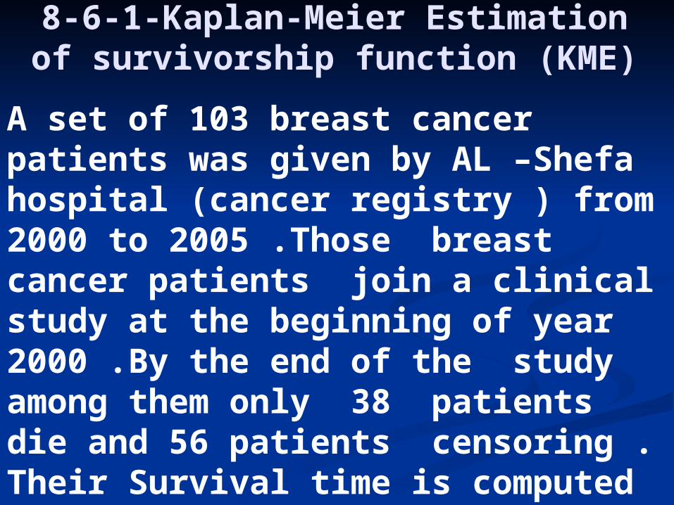
8-6-1-Kaplan-Meier Estimation of survivorship function (KME)

A set of 103 breast cancer patients was given by AL –Shefa hospital (cancer registry ) from 2000 to 2005 .Those breast cancer patients join a clinical study at the beginning of year 2000 .By the end of the study among them only 38 patients die and 56 patients censoring . Their Survival time is computed from time of diagnosis in days . Table (1) below lists the survival times t in days for those cases who die by the end of the study .

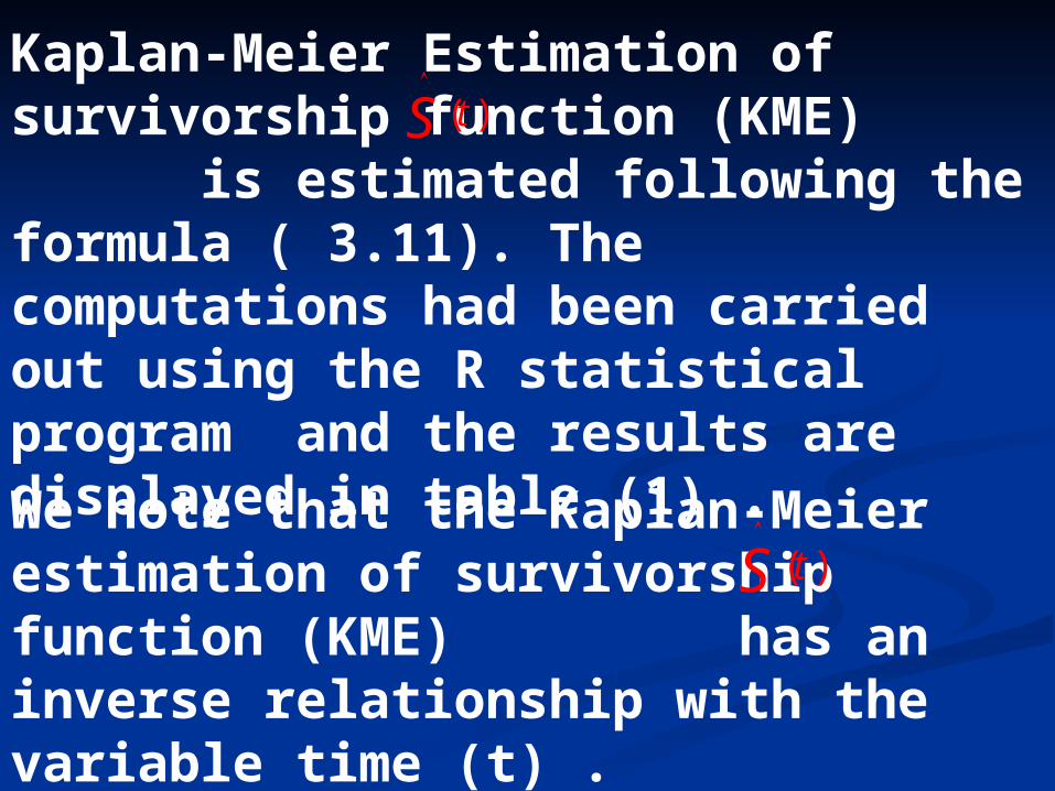
Kaplan-Meier Estimation of survivorship function (KME) is estimated following the formula ( 3.11). The computations had been carried out using the R statistical program and the results are displayed in table (1) .

( )tS

We note that the Kaplan-Meier estimation of survivorship function (KME) has an inverse relationship with the variable time (t) .

( )tS

Similar to other estimators, the standard error (S.E.) of the Kaplan Meier estimator of

gives an indication of the potential error of by formula (3.16) , The confidence interval deserves more attention than just the point estimate . A 95% confidence interval for is estimated by .This also has been calculated using the R program , and the results are illustrated in table (1) .

( )tS

( )tS

( )tS

( )tS

( ) 1.96 . .[ ]( )t S E S tS

Table (1 ),Kaplan-Meier Estimation of survivorship function (KME)

Estimate

NODAYSSTATUSCUMULATIVE PROPORTION SURVIVING AT THE TIME

LOWER 95% CI

UPPER 95% CI

HAZARD

Std. Error

152event.990.0100.9721.0000.0098

272event.981.0140.9541.0000.0196

3221event.971.0170.9391.0000.0296

4281event.961.0190.9250.9990.0396

5355event.951.0210.9110.9940.04976

6447event.942.0230.8980.9880.060

7528event.932.0250.8850.9820.0703

8596event.922.0260.8720.9750.0809

9609event.913.0280.8600.9690.0914

10626event.903.0290.8480.9620.10213

11680event.893.0300.8360.9550.1129

12748event.883.0320.8240.9480.12387

13754event.874.0330.8120.9400.13492

14767event.864.0340.8000.9330.1461

15802event.854.0350.7890.9250.1574

16806event.845.0360.7780.9180.1688

17810event.835.0370.7660.9100.1804

Estimate ( )tS

NODAYSSTATUSCUMULATIVE PROPORTION SURVIVING AT THE TIME

LOWER 95% CI

UPPER 95% CI

HAZARD

Std. Error

18883event.825.0370.7550.9020.1921

19892event.816.0380.7440.8940.2039

20893event.806.0390.7330.8860.21589

21929event.796.0400.7220.8780.2280

22968event.786.0400.7110.8700.2403

231.002E3event.777.0410.7000.8610.2527

241.247E3event.767.0420.6900.8530.2653

251.413E3event.757.0420.6790.8450.2780

261.492E3event.748.0430.6680.8360.2909

271.503E3event.738.0430.6580.8280.30399

281.608E3event.728.0440.6470.8190.3172

291.660E3event.718.0440.6370.8110.3307

301.733E3event.709.0450.6260.8020.3443

311.757E3event.699.0450.6160.7930.3581

321.792E3event.689.0460.6060.7850.372

331.839E3event.679.0460.5940.7750.3878

341.893E3event.667.0470.5810.7650.4055

351.946E3event.653.0480.5660.7540.4261

362.048E3event.622.0550.5230.7390.4749

372.106E3event.574.0680.4550.7250.55495

382.140E3event.492.0960.3360.7210.7091

Estimate ( )tS

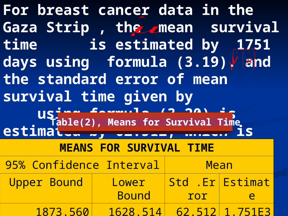
For breast cancer data in the Gaza Strip , the mean survival time is estimated by 1751 days using formula (3.19). and the standard error of mean survival time given by using formula (3.20) is estimated by 62.512, which is indicated in table (2).

V

Table(2), Means for Survival Time

MEANS FOR SURVIVAL TIME

Mean95% Confidence Interval

EstimateStd .ErrorLower BoundUpper Bound

1.751E362.5121628.5141873.560

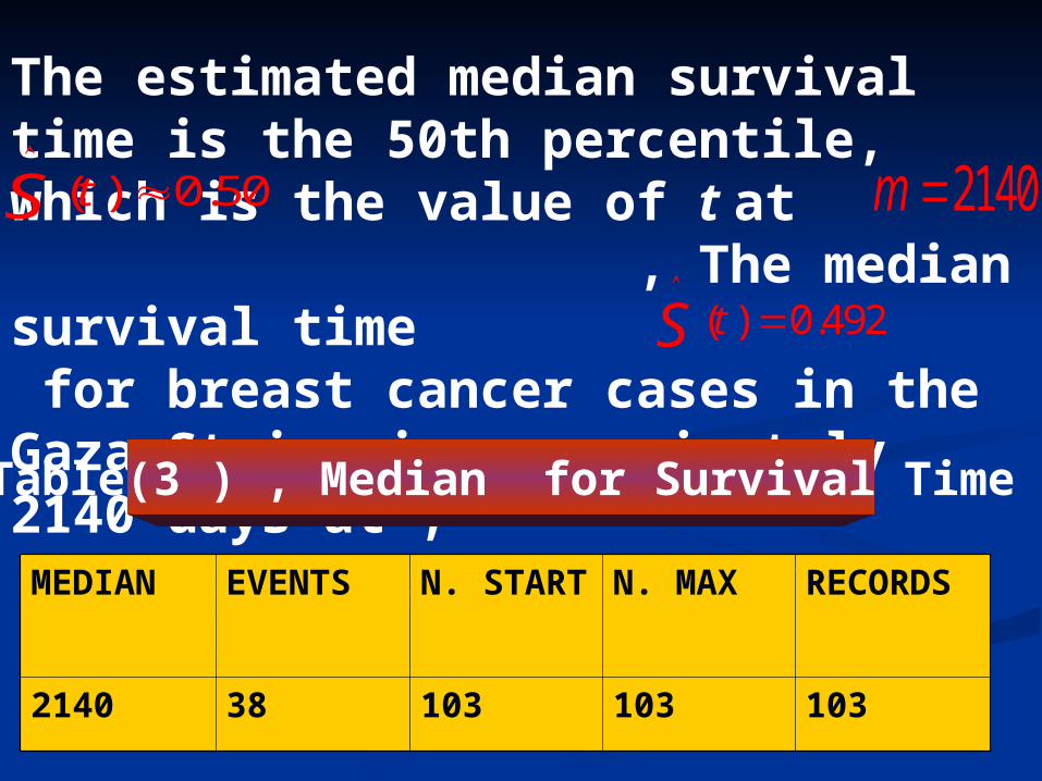
The estimated median survival time is the 50th percentile, which is the value of t at , The median survival time for breast cancer cases in the Gaza Strip is approximately 2140 days at , which is indicated in table (3) below .

( ) 0.50tS

2140m

( ) 0.492tS

Table(3 ) , Median for Survival Time

RECORDSN. MAXN. STARTEVENTSMEDIAN

103103103382140

Theoretically ,the estimator of survival function which is plotted in graph (1) is expected to appears as a step function since it remains constant between two observed exact survival times. However, The most commonly used summary statistic in survival analysis is the median survival time. The median survival time ( =2140 days ) is estimated from the survival curve . The estimated mean survival time( =1751 days ) can be seen to equal the area under the estimated survivorship function as described by formula (3.18).

( )tS

m

Graph (1 ) , Kaplan-Meier estimate of the survivorship function for the data in Table (1) and its 95% confidence intervals .

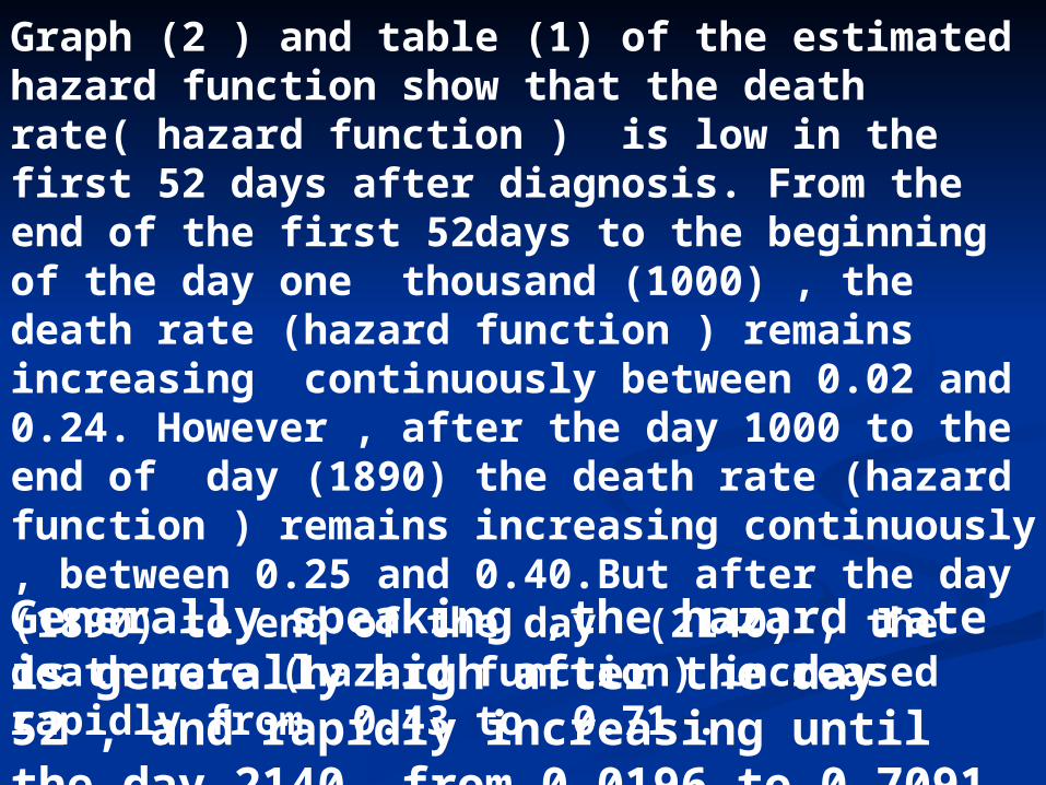
Graph (2 ) and table (1) of the estimated hazard function show that the death rate( hazard function ) is low in the first 52 days after diagnosis. From the end of the first 52days to the beginning of the day one thousand (1000) , the death rate (hazard function ) remains increasing continuously between 0.02 and 0.24. However , after the day 1000 to the end of day (1890) the death rate (hazard function ) remains increasing continuously , between 0.25 and 0.40.But after the day (1890) to end of the day (2140) , the death rate (hazard function) increased rapidly from 0.43 to 0.71 .

Generally speaking ,the hazard rate is generally high after the day 52 , and rapidly increasing until the day 2140 from 0.0196 to 0.7091

Graph (2) Hazard function for breast cancer patients in the Gaza Strip.

8-6-2-The Log–Rank test for Comparison of two Survival Distributions

The problem here is to compare survival times of two groups of patients of breast cancer exposed to four different treatments ( Surgery, Radiotherapy ,Chemotherapy, Hormonal Therapy) by comparing the survivorship function and hazard function of the two groups .

The following survival data for 103 females with breast cancer , contains two groups , the first group contains the patients of ages less than 50 years old and the second group contains patients with ages greater or equal to 50 years old .

Survival times are estimated for both groups from time of diagnosis in days . Table (4) lists the survival times t in days .

Kaplan-Meier Estimation of survivorship function (KME) is computed , in table(4) .

( )tS

( )tS

( )tS

Similar to other estimators, the standard error (S.E.) of the Kaplan Meier estimator of and A 95% confidence interval for is also estimated in table (4) .

( ) 1.96 . .[ ]( )t S E S tS

Table (4) ,Kaplan-Meier Estimation of survivorship function (KME) for two groupsof breast cancer cases in the Gaza Strip.

NODAYSSTATUSCUMULATIVE PROPORTION

SURVIVING AT THE TIME

LOWER 95% CI

UPPER 95% CI

DIFFERENCEHAZARD

Std. Error

1447event0.9710.0290.914161.02784less than 50 0.0299

2528event0.9410.040.86261.0194less than 50 0.061

3609event0.9120.0490.815961.00804less than 50 0.0921

4748event0.8820.0550.77420.9898less than 50 0.1252

5754event0.8530.0610.733440.97256less than 50 0.1592

6767event0.8240.0650.69660.9514less than 50 0.1942

7806event0.7940.0690.658760.92924less than 50 0.231

8883event0.7650.0730.621920.90808less than 50 0.2683

9892event0.7350.0760.586040.88396less than 50 0.310

10893event0.7060.0780.553120.85888less than 50 0.348

11968event0.6760.080.51920.8328less than 50 0.391

121.00E+03event0.6470.0820.486280.80772less than 50 0.435

131.25E+03event0.6180.0830.455320.78068less than 50 0.482

141.61E+03event0.5880.0840.423360.75264less than 50 0.531

151.66E+03event0.5590.0850.39240.7256less than 50 0.582

161.76E+03event0.5290.0860.360440.69756less than 50 0.636

171.79E+03event0.50.0860.331440.66856less than 50 0.6932

Estimate ( )S t

NODAYSSTATUSCUMULATIVE PROPORTION

SURVIVING AT THE TIME

LOWER 95% CI

UPPER 95% CI

DIFFERENCEHAZARD

Std. Error

182.11E+03event0.4170.1040.213160.62084less than 50 0.8755

192.14E+03event0.3120.1190.078760.54524less than 50 1.1632

2052event0.9860.0140.958561.01344greater or equal 500.0146











311.41E+03event0.8260.0460.735840.91616greater or equal 500.19106








Estimate ( )S t

The estimated mean survival time for the first group is 1583 days , and the standard error of the mean survival time is 109.04 .

1

1V

However , the estimated mean survival time or the second group is 1832, and the standard error of the mean survival time is 74.23.

2

2V

Moreover , the estimated mean survival time for all patients is 1751 days and the standard error of the mean survival time for all patients is 62.512 .The above results are illustrated in table (5) below.

V

Table (5) , Means for Survival Time for two groups of breast cancer in the Gaza Strip

DIFERENTMEAN

EstimateStd. Error95% Confidence Interval

Lower BoundUpper Bound

less501.583E3109.0421369.3751796.818

more501.832E374.2331686.6441977.638

Overall1.751E362.5121628.5141873.560

For the remission data, the log–rank statistic computed using formula (3.24), is 6.004 and indicated in table (6) and the corresponding P-value is .014 which indicates that the null hypothesis should be rejected .The null hypothesis being tested is that there is no overall difference between the two survival curves . We can therefore conclude that the first group and the second group are significantly different (KME) survival curves.

Table (6) , Test of equality of survival distributions for the different levels of different by Log Rank test

OVERALL COMPARISONS

Chi-SquaredfSig.

Log Rank (Mantel-Cox)

6.0041.014

Now, plots of the (KME) curves for the first group together with the second group are shown here in the graph (3) below. Notice that the (KME) curve for the second group is consistently higher than the (KME) curve for the first group . These results indicate that the second group , has better survival and better response to treatment than first group .

Moreover, as the number of days increases, the two curves appear to get further apart, which indicate that the effect of treatment on the second group is greater than the effect of treatment on the first group to stay in remission.

Graph (3) , Kaplan-Meier estimate of the survivorship function for the data in table (5.24) for two groups

The graph (4) of the estimated hazard function shows that the death rate for both groups are low in the first 750 days after diagnosis. After 750 days to the end , the death rate remains increasing continuously for both groups , but the first group contains patients with ages less than 50 years old with death rates between ( 0.13 - 0.70) while the second group contains patients with ages greater or equal to 50 years old with death rates between ( 0.14 - 0.40).

The hazard rate is generally high and increase continuously for first and second group , but the hazard rate for the first group is higher than the second group .Notice that the second group contains patients who have ages greater or equal to 50 years old .

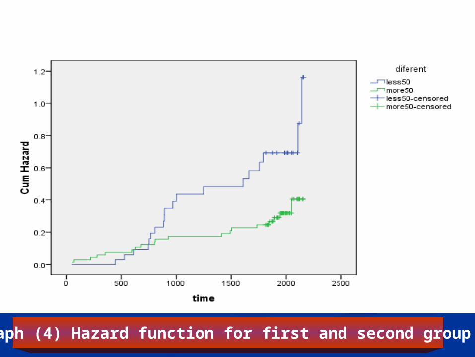
Graph (4) Hazard function for first and second group

8-6-3-Cox Proportional Hazards Model (CPHM)

8-6-3-1-The Formula for the Cox Proportional Hazards Model

We are thus considering a problem involving four explanatory variables as predictors of survival time T, where T denotes days until going out of remission “death” and we label the explanatory variables (two groups of breast cancer patients) , with 34 patients in the first group which contains the patients with ages less than 50 years old and 69 patients in the second group which contains patients who have ages greater or equal to 50 years old .

1X

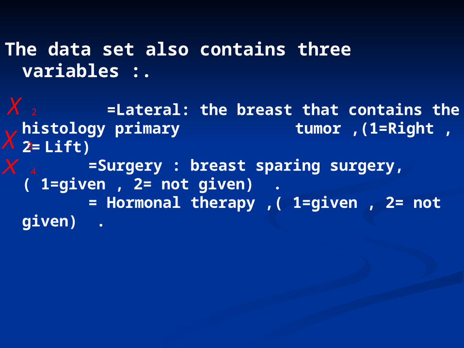
The data set also contains three variables :.

=Lateral: the breast that contains the histology primary tumor ,(1=Right , 2= Lift)

=Surgery : breast sparing surgery, ( 1=given , 2= not given) . = Hormonal therapy ,( 1=given , 2= not given) .

2X

3X4X

The outcome variable for the model is the time in days until a patient goes out of remission (died).

We have been described the final model and their results concerning breast cancer cases in the Gaza Strip.

We now describe final model and their results concerning breast cancer cases in the Gaza Strip

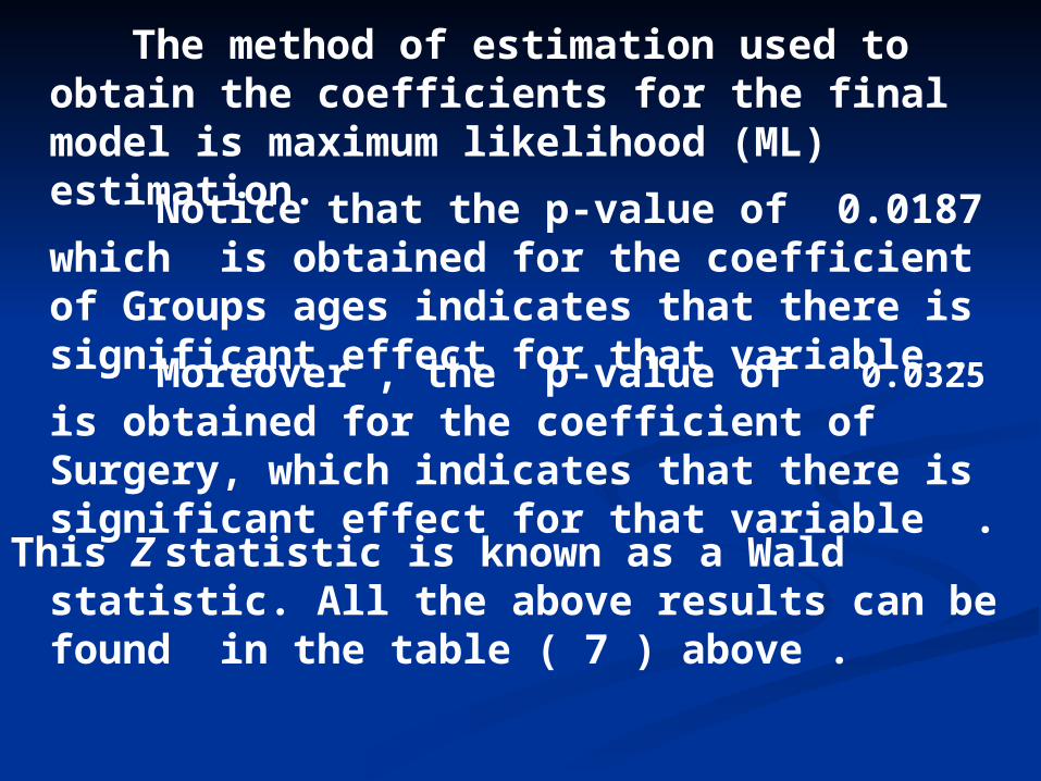
The method of estimation used to obtain the coefficients for the final model is maximum likelihood (ML) estimation.

Notice that the p-value of 0.0187 which is obtained for the coefficient of Groups ages indicates that there is significant effect for that variable .

Moreover , the p-value of 0.0325 is obtained for the coefficient of Surgery, which indicates that there is significant effect for that variable .

This Z statistic is known as a Wald statistic. All the above results can be found in the table ( 7 ) above .

Table(7) Variables in the equation

COEFHRSE(COEF)ZLOWER.95UPPER .95

Groups Ages0.7695-0.46320.3273-2.3510.01810.24390.8798

Surgery-1.0370.35450.48492.139-0.03250.13710.917

likelihood = - 157.9798

( )r

ZP

Finally ,we consider final model for the remission data. The fitted model written in terms of the hazard function using formula (4.1) is given by.

0.77Groups Age-1.04Surgery0

ˆ ˆ( , , ) ( )h t B h t e

8-6-3-2-Adjusted Survival Curves Using the 8-6-3-2-Adjusted Survival Curves Using the (CPHM) (CPHM)

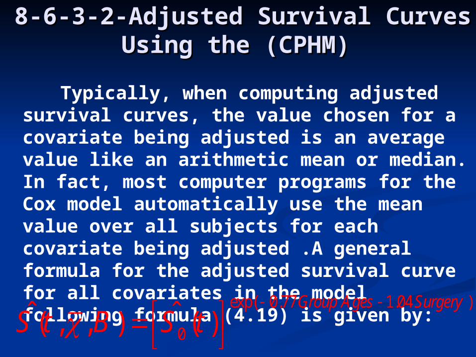
Typically, when computing adjusted survival curves, the value chosen for a covariate being adjusted is an average value like an arithmetic mean or median. In fact, most computer programs for the Cox model automatically use the mean value over all subjects for each covariate being adjusted .A general formula for the adjusted survival curve for all covariates in the model following formula (4.19) is given by:

exp( 0.77 1.04 )

0ˆ ˆ( , , ) ( )

Group Ages Surgery

S t B S t

To obtain the adjusted survival curve, we then substitute the mean values in the formula in the model fitted. The formula and the resulting expression for the adjusted survival curve are shown below and the results of application of the adjusted survival carve are given in the third column of the table (8)

0.0377

0ˆ ˆ( , , ) ( )S t B S t

Table (8) , Adjusted Survival function Using the Cox PH Model

NOTIMESURVIVALS.ELOWER 95% CI

UPPER 95% CI

Baseline Cum Hazard

Baseline survivorship function

Cumulative hazard function

1520.9910.0090.97510.2280.79630.009

2720.9830.0120.9610.4570.63320.017

32210.9740.0150.94710.6880.502780.026

42810.9660.0170.93410.9210.398130.035

53550.9570.0190.9220.9951.1590.313920.044

64470.9490.0210.910.9911.40.246580.053

75280.940.0220.8980.9861.6480.192390.062

85960.9310.0240.8860.981.9020.149210.072

96090.9220.0260.8740.9742.1590.11540.081

106260.9130.0270.8630.9682.4190.0890.091

116800.9040.0280.8510.9622.6810.068510.101

127480.8950.030.840.9562.9450.052590.111

137540.8860.0310.8290.9493.2140.04020.121

147670.8770.0320.8180.9433.4870.030590.131

158020.8680.0330.8070.9363.7630.023210.142

168060.8590.0340.7960.9294.0430.017550.152

178100.850.0350.7850.9224.3250.013230.163

188830.840.0360.7740.9154.6120.009930.174

0( )tH ( )0 tS

( , , )H t x B

NOTIMESURVIVALS.ELOWER 95% CI

UPPER 95% CI

Baseline Cum Hazard

Baseline survivorship function

Cumulative hazard function

198920.8310.0370.7630.9084.9070.007390.185

208930.8220.0380.7520.9015.2130.005440.196

219290.8120.0390.7420.8935.5230.003990.208

229680.8030.0390.7310.8865.8370.002920.22

2310020.7930.040.720.8786.1570.002120.232

2412470.7830.0410.7090.876.4830.001530.244

2514130.7740.0420.6980.8626.8130.00110.257

2614920.7640.0420.6870.8547.1460.000790.269

2715030.7540.0430.6770.8467.4860.000560.282

2816080.7440.0440.6660.8387.8330.00040.295

2916600.7350.0440.6550.838.1870.000280.309

3017330.7250.0450.6440.8228.5470.000190.322

3117570.7150.0460.6340.8138.9120.000130.336

3217920.7050.0460.6230.8059.2859.3E-050.35

3318390.6940.0470.6110.7959.6996.1E-050.365

3418930.6810.0480.5970.78510.23.7E-050.384

3519460.6670.0490.5810.77410.762.1E-050.406

3620480.6390.0550.5460.7611.96.8E-060.448

3721060.5930.0660.4870.74813.869.5E-070.522

3821400.5190.0870.3930.74117.392.8E-080.655

0( )tH ( )0 tS

( , , )H t x B

Graph (5) adjusted survival curves obtained from fitting a Cox model

9-The recommendations

1- We recommend reactivation and rehabilitation of the Cancer Registry Center in Palestine to know the exact oncology cases and its different diagnostic sources in order to define the problem and its spreading reasons .

2- Develop the use of (Ten International Classification ICD10) which is related to diseases , deaths and disabled people . Using such kind of classification required training for doctors, health professionals and data entry persons.

3- We recommend establishing an advanced system for record registry of causes of death on death certificates.

4- Development of cooperation and full coordination between system and information Department and Cancer Registry Center for monitoring and recording of cases of tumors in the Ministry of Health through a sophisticated electronic system.

5- It is important to develop the Cancer Patients data in cancer Registry Center . Furthermore , it is required to improve the cooperation between Ministry of Health and Palestinian Central Bureau of Statistics to minimize the gaps of indicators which depend on the Ministry of health data and estimated indicators of the PCBS which come as a result of health surveys .

6- We recommend applying the Kaplan-Meier Estimation of survivorship function (KME ) and estimated mean survival time for all cancer patient with confidence interval for .( )tS

( )tS

7- We recommend the determination of the relationship between (KME ) and time for all cancer patients and determination of the relationship between hazard ratio and time for all cancer patients, using the statistics program R.

8- A clinical oncologist may be interested in comparing the ability of two or more treatments to prolong life or maintain health for two group from patients ages . Almost invariably, survival times of the different groups vary. Therefore, we recommend using the Log–Rank Test For Comparison of two survival distributions for all cancer patients.

9- We recommend using the Cox proportional hazards model (CPHM), for analyzing survival data , that contain the most important variables as predictors of survival time T, where T denotes days until going out of remission “death or survive”, for all cancer patients in Palestine.

قال رسول الله صلى الله :عليه وسلم

إن الله يحب إذا عمل أحدكم عمال )) .((أن يتقنه

faculty of economics and administrative sciences department of applied statistics survival analysis...

Documents

individual survival

survival distributions

introduction survival

survival analysis techniques

survival analyses

survival of groups

survival curve estimates

data analysis