factors affecting the adoption of wind and solar - … affecting the adoption of wind and ... and...
TRANSCRIPT
Office of Energy Policy and New Uses Office of the Chief Economist
U.S. Department of Agriculture
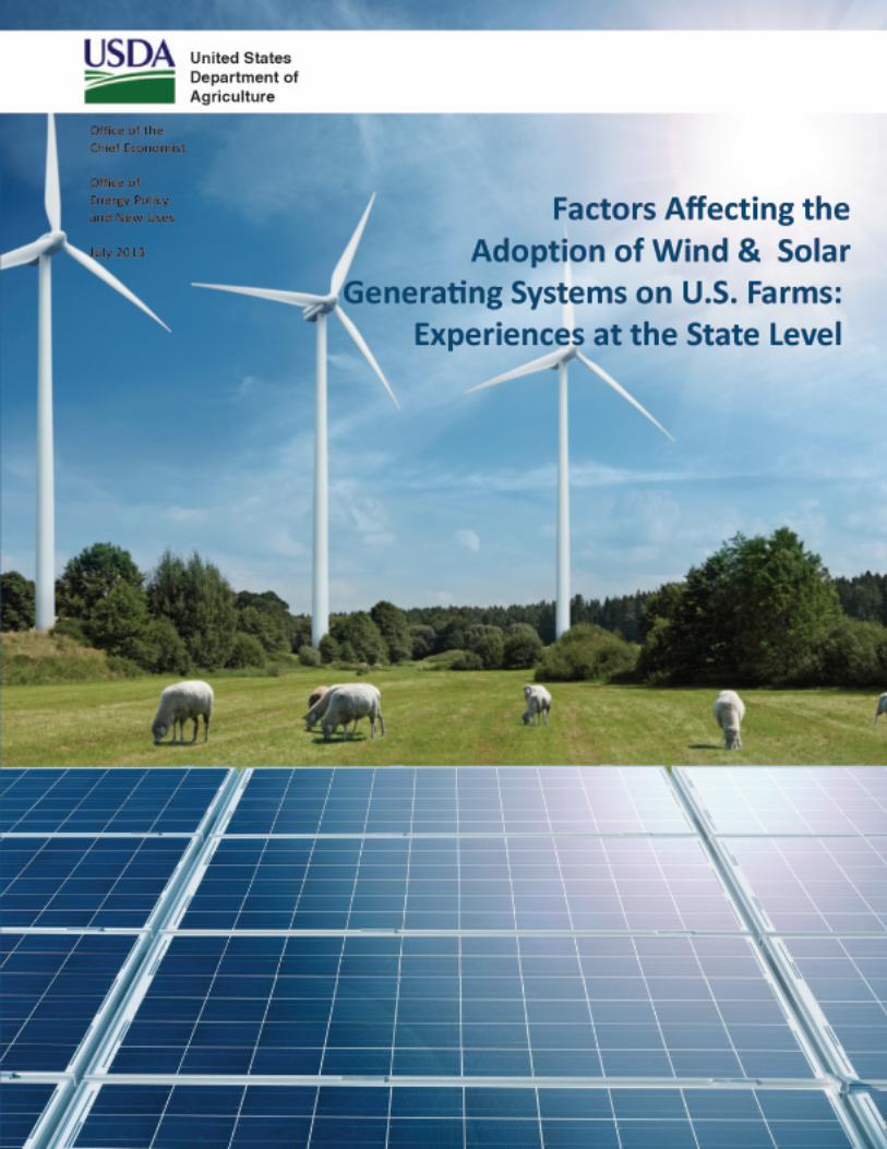
Factors Affecting the Adoption of Wind and
Solar-Power Generating Systems on U.S. Farms:
Experiences at the State Level
Irene M. Xiarchos, Natural Resource Economist and Policy Analyst, Office of Energy Policy and New Uses, Office of the Chief Economist, U.S. Department of Agriculture William Lazarus, Professor and Extension Economist, Department of Applied Economics, University of Minnesota

Contents
Executive Summary
1
Introduction
Literature Review
Solar and Wind Electricity on U.S. Farms
2
5
8
Factors Influencing Solar and Wind System Adoption on Farms
14
Modeling Aggregate Renewable Electricity Adoption
27
Summary and Conclusion
33
References
35
Tables and Figures Tables
Table 1. Farms with Solar Photovoltaic (PV) by State 9
Table 2. Farms with Small Wind by State 10
Table 3. Lowest and Highest Average Installation Cost by State 12
Table 4. Correlation Analysis for Policy Variables With Solar-PV and Small Wind
Adoption Rates
18
Table 5. Test of Means of Solar-Photovoltaic (PV) and Small-Wind Adoption Rates for
Renewable Portfolio Standard (RPS)
19
Table 6. Test of Means of Solar-Photovoltaic (PV) and Small-Wind Adoption Rates for
Net Metering
21
Table 7. Test of Means of Solar-Photovoltaic (PV) and Small-Wind Adoption Rates for
Interconnection
22
Table 8. Select Policy Variables for the U.S. States 24
Table 9. Correlation Analysis for State Agricultural Characteristics with Solar-PV and
Small-Wind Adoption Rates
26
Table 10. Modeling Results for Solar-Photovoltaic (PV) Adoption Rates 30
Table 11. Modeling Results for Small Wind Adoption Rates 31
Table 12. Normality Test for 2005 Logit Transformation Regression Models 32
Figures
Figure 1. Renewable Share of Net Electricity Generation by State (excludes Hydroelectric) 2
Figure 2. State Adoption Shares for Photovoltaic Solar and Small Wind 10
Figure 3. Increase in Electricity Price Required for Residential PV Breakeven at $8/Watt 13
Figure 4. Kernel Density Plots for the Share of Farms with Solar-Photovoltaic (PV) and
Small-Wind Installations Before and After the Logit Transformation
27
Acknowledgements
We appreciate the reviews from Robert Yohansson at USDA’s Office of the Chief
Economist (OCE); Harry Baumes at USDA’s Office of Energy Policy New Uses
(OEPNU); Jan Lewandrowski at USDA’s Climate Change Program Office (CCPO);
Donald Buysse, and Dale Hawks at USDA’s National Agricultural Statistics Service
(NASS); Hansen LeRoy, and Peter Stenberg at USDA’s Economic Research Service
(ERS); Antony Crooks at USDA’s Rural Development (RD); David Buland at USDA’s
Natural Resource Conservation Service (NRCS); and John Hay at the University of
Nebraska. Further contributions we would like to acknowledge include input from
Charlie Hallahan and Allison Borchers at USDA’s Economic Research Service (ERS),
Faye Propsom at USDA’s National Agricultural Statistics Service (NASS), and Antony
Crooks at USDA’s Rural Development (RD). We also appreciate the design assistance
from Jennifer Lohr and Brenda Chapin at USDA’s Office of the Chief Economist (OCE).
Executive Summary 1 |
Executive Summary
The study is the first to examine the role of State-level policies such as net metering and
Renewable Portfolio Standards (RPS), as well as the role of electric cooperatives, on
States’ adoption rates of solar and wind systems on U.S. farms. The study found that
States with higher energy prices, more organic acres per farm, and more Internet
connectivity adopt renewable electricity at higher rates. For solar systems, full farm
ownership and solar resources also have a significant and positive relationship with
adoption rates.
RPS targets are found to increase renewable electricity adoption at the State level. Our
result accords with the literature; however, this is the first study to show an impact at the
distributed-generation scale. Our study does not find a systematic relationship for State
financial instruments, such as rebates, grants, investment tax credits, and production
incentives, at least in the form captured by our policy variables. Similarly, net metering
and interconnection policies do not seem to influence renewable electricity adoption at
the State level. Conversely, electric cooperative prevalence in the State is found to have a
negative relationship to renewable electricity adoption share. The interaction of those
factors highlights the importance of coordinating approaches in policy formulation to
meet Federal and State objectives of increasing renewable energy adoption.
The results of this study can assist States as they further refine and focus their policies to
promote renewable electricity, particularly during an era of declining government
budgets. A more detailed examination of farm-level data from the On-Farm Renewable
Energy Production Survey in combination with policy, institutional, and economic
variables at the State level can provide a fuller and more realistic interpretation of the
State-level determinants of adoption of wind- and solar-energy technologies.
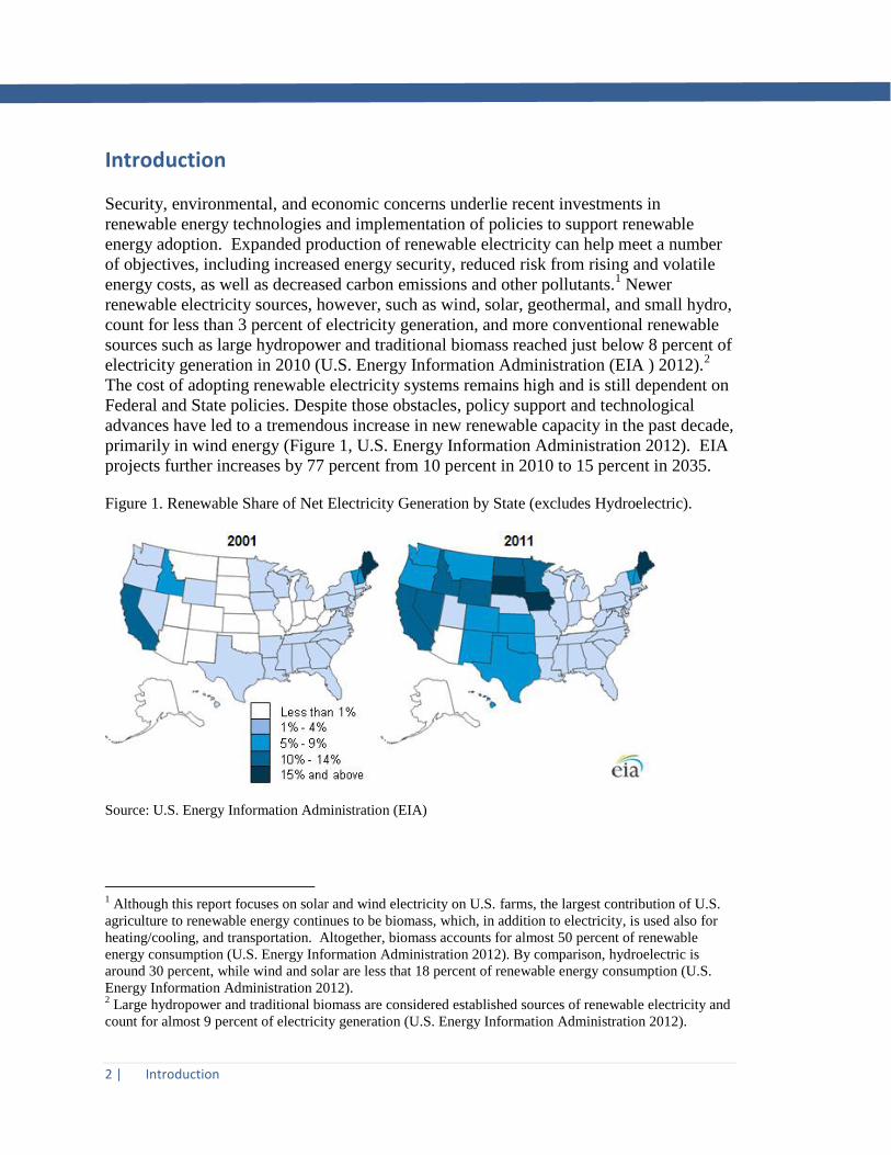
2 | Introduction
Introduction
Security, environmental, and economic concerns underlie recent investments in
renewable energy technologies and implementation of policies to support renewable
energy adoption. Expanded production of renewable electricity can help meet a number
of objectives, including increased energy security, reduced risk from rising and volatile
energy costs, as well as decreased carbon emissions and other pollutants.1 Newer
renewable electricity sources, however, such as wind, solar, geothermal, and small hydro,
count for less than 3 percent of electricity generation, and more conventional renewable
sources such as large hydropower and traditional biomass reached just below 8 percent of
electricity generation in 2010 (U.S. Energy Information Administration (EIA ) 2012).2
The cost of adopting renewable electricity systems remains high and is still dependent on
Federal and State policies. Despite those obstacles, policy support and technological
advances have led to a tremendous increase in new renewable capacity in the past decade,
primarily in wind energy (Figure 1, U.S. Energy Information Administration 2012). EIA
projects further increases by 77 percent from 10 percent in 2010 to 15 percent in 2035.
Figure 1. Renewable Share of Net Electricity Generation by State (excludes Hydroelectric).
Source: U.S. Energy Information Administration (EIA)
1 Although this report focuses on solar and wind electricity on U.S. farms, the largest contribution of U.S.
agriculture to renewable energy continues to be biomass, which, in addition to electricity, is used also for
heating/cooling, and transportation. Altogether, biomass accounts for almost 50 percent of renewable
energy consumption (U.S. Energy Information Administration 2012). By comparison, hydroelectric is
around 30 percent, while wind and solar are less that 18 percent of renewable energy consumption (U.S.
Energy Information Administration 2012). 2 Large hydropower and traditional biomass are considered established sources of renewable electricity and
count for almost 9 percent of electricity generation (U.S. Energy Information Administration 2012).
Introduction 3 |
Wind and solar installations are often located on or close to agricultural land. For that reason,
and because 40 percent of the total U.S. land area is in agriculture, many leading States in
renewable electricity installations are States with large agricultural sectors (National
Agricultural Statistics Service, 2009a).1 Farming operations are also a natural fit for smaller
scale renewable electricity applications. Agricultural producers are actually early adopters of
renewable powered technology due to its convenience for small and remote power needs.
Wind turbines, for example, were used to pump water and for remote electricity generation
since the early 1900s and, in the absence of rural electrification, were widely incorporated in
agriculture operations by 1930.
At the time, agriculture represented the main market for wind energy systems and
continues to present a large market opportunity for sales of small wind systems (less than
100 kilowatts) today (American Wind Energy Association 2011). Stand-alone solar
photo-voltaic (PV) systems were introduced in the 1980s and have become the most
common form of on-farm electricity generation (National Agricultural Statistics Service
2011). Though those off-grid applications represented the majority of renewable energy
use throughout the 1990s, grid-connected systems are now leading the growth in on-farm
systems (Xiarchos and Vick 2011).
The 2009 On-Farm Renewable Energy Production Survey (OFREPS) was the first
national survey of on-farm renewable energy generation. It addressed only distributed
generation of on-farm renewable energy applications owned and operated as part of
individual farm operations.3 It excluded “large wind” systems of 100 kilowatts or more,
which are generally commercial applications often located on farms but operated by other
business entities under wind rights lease agreements with the farm (National Agricultural
Statistics Service 2011).4 The number of small wind systems has almost doubled since
2001 (American Wind Energy Association 2011), while solar power has increased by 146
percent since 2000 (Sherwood 2010).5 The OFREPS survey provides insights about
renewable electricity in agriculture and factors that influence distributed generation.
Following the examples of Menz and Vachon (2006), Adelaja and Hailu (2008), and
Sawyer, et al. (1984), our examination applies specifically to State-level adoption rates of
wind and solar systems for farms and evaluates the State factors that might explain the
3 Distributed generation (DG) is an approach that employs small-scale technologies to produce electricity
close to the end users of power. DG technologies often consist of modular (and sometimes renewable-
energy) generators and provide power onsite with little reliance on the distribution and transmission grid.
DG can often provide lower-cost electricity and higher power reliability and security with fewer
environmental consequences than can traditional power generators. 4 This report focuses on wind and solar installations captured in the OFREPS (available at
http://www.agcensus.usda.gov/Publications/Energy_Production_Survey/). It excludes anaerobic digesters
(also included in the OFREPS), as well as small hydro, and geothermal systems (not examined in the
OFREPS). 5 Until 2009, which frames the study period of the paper, most of the PV installations had been customer
sited. 2010 marks the emergence of the utility sector in PV. The share of utility sector installations rose
from virtually none in 2006 to 15 percent of all installations in 2009 and 32 percent in 2010 (Sherwood
2010).

4 | Introduction
States’ varying adoption rates.6 Our main interest lies in identifying policy and
institutional influences on State-level adoption differences while controlling for State
differences in economics and structural factors in agriculture. The interest on policy
variables is nested in the perceived importance of policy in promoting renewable
electricity technologies until volume-related costs reach parity with fossil-based
technologies. That study is unique in that it focuses on distributed generation on farms,
whereas previous State-level work focused primarily on utility-scale installations (Menz
and Vachon 2006, Adelaja and Hailu 2008, Yin and Powers, 2010, Shrimali and Kniefel
2011). Small-scale renewables have, up to now, mostly been examined at the household
level (Mills and Schleich 2009, Durham et al. 1988, Labay and Kinnear 1981, Willis et
al. 2011).
To identify a range of potential factors that might systematically account for State
variations, bivariate statistical correlation tests are performed in accordance to Sawyer et
al. (1984). Variables that show a significant relationship are used to construct a
parsimonious multivariate representation of those relationships in the absence of multi-
period observations following Menz and Vachon (2006) and Adelaja and Hailu (2008).
Although technology adoption is ultimately an individual farm-level choice, analyzing
State-level variables can help explain underlying State variation and evaluate policy
effectiveness.
6 The term adoption rate herein refers to the proportion of farms in each State that installed renewable
electricity systems on their operation until 2009, based on the OFREPS survey.

Literature Review 5 |
Literature Review
The literature on for renewable electricity varies in at least four ways:
1. Technologies analyzed.
2. Level of aggregation (individual decisionmaker or State-level totals)
examined.
3. Sector (utilities, residential users, or farm operators) evaluated.
4. Analytical methods used to evaluate adoption (ordinary least squares
regression, limited dependent variable regression, other statistical
technique, or simulation).
Analytical methods used in renewable energy adoption research can be characterized as
statistical and non-statistical. Most recent statistical technology adoption research has
focused on total renewable electricity capacity or generation in the State. At aggregate
levels, utility-scale capacity overshadows distributed generation by end-users such as
farmers, and consequently, total renewable electricity capacity represents utility-scale
capacity in those studies. State-level studies face the disadvantage of relying on
secondary data, while studies of individual decisionmakers use data from surveys
designed specifically for that purpose. Also, State-level studies generally involve fewer
degrees of freedom and narrower ranges of values for the variables, so that consequently
they are less likely to find statistically significant results.
Menz and Vachon (2006) was the first State-level evaluation of how utility-scale
renewable electricity capacity relates to State policies. They examined the impact of an
array of government policies in 39 States on wind energy capacity and its growth from
1998-2003 through hierarchical linear regression analysis. They considered renewable
portfolio standards (RPS), generation disclosure, a mandatory green power option, public
benefit funds, and choice of electricity source. Their study was conducted in two parts.
The first part used bivariate variables for the above policies in existence prior to 2003.
The second part used the experience related to each policy expressed as the time since
each policy enactment. They found that both renewable portfolio standards (RPS) and
green power options were positively related to wind power development. Adelaja and
Hailu (2008) furthered the analysis by adding State socioeconomic and political
characteristics in addition to renewable energy policies in the examination of State
differentials in wind industry development. That study found that RPS has a significant
effect on wind development as do the State’s wind potential, economic conditions, and
political structure.
Yin and Powers (2010) evaluated by means of a fixed effects panel model the presence of
an RPS and its stringency (as measured by whether some utilities in the State are exempt
from the RPS, whether existing generation when the RPS is implemented is allowed to
“count” against the RPS, whether utilities can purchase renewable electricity credits from
outside the State to meet part of the RPS, and penalties imposed on non-compliant energy
6 | Literature Review
producers). They found that an RPS that requires additional renewable generation above
that existing at implementation has a positive impact where the mere presence of a
weaker RPS does not. Net metering and interconnection were not found to be effective in
increasing renewable generation, while mandatory green power offerings and greater
imported power had positive and significant impacts.
Shrimali and Kniefel (2011) consider the impact of RPS, government green power
purchasing, and financial incentives along with resource, economic, and political
measures on wind, biomass, geothermal, and solar generation capacity. They used a
fixed-effects model with State-specific time-trends for State-level data from 1991-2007
and found that RPS impact varied by type of renewable and was negative for combined
renewables. It was positive for solar and geothermal and negative for wind and biomass.
They also found that clean energy funds have a significant impact on the share of
renewable energy, while previous literature showed that a related policy, public benefit
funds, was not significant.
Delmas and Montes-Sancho (2011) focused on determinants at the utility rather than the
State level. They found that the RPS has a negative influence on utilities’ decision to
invest in renewable capacity and that investor-owned utilities respond more positively to
RPS mandates than publicly owned utilities. They consider the possibility that renewable
capacity expansion may be due to the natural, social, and policy context in the State
rather than due to the RPS, resulting in “sample selection” bias. They employ a two-
stage Heckman approach with a logit model predicting RPS adoption and then use the
predicted RPS in a Tobit model of capacity.
Adoption of distributed generation for residential and small commercial entities is likely
to differ from utility-scale generation. For example, renewable energy technologies
adopted by farmers usually represent only a small part of the farm business and produce
electricity mainly for consumption on the farm, in contrast to renewable energy
technologies adopted by utilities whose main product is electricity for sale to the public in
the marketplace.
Sawyer et al. (1984) performed a State-level analysis for distributed generation;
specifically, they used a statistical approach to examining how adoption rates for
residential solar installations have varied across States. They conducted bivariate
statistical correlation tests of 11 independent variables with solar adoption rates. They
also found that actual adoption was low even where it was expected to be economically
feasible. They attributed the low adoption rates to consumers being more concerned with
time to pay back the investment rather than the overall life-cycle cost criterion that had
been used in the projections. Anticipating Delmas and Montes-Sancho’s concern about
causation and sample selection bias, Sawyer et al. included an index of regional
differences in cultural attitudes toward adoption of policy innovations and alteration of
established patterns.
At the household level in the residential sector, economic variables shown to impact solar
hot water adoption choices have included solar radiation availability (Mills and Schleich

Literature Review 7 |
2009), electricity rates (Fujii and Mak, 1984; Durham et al., 1988), and State tax credits
(Durham et al. 1988). Demographic variables that positively related to energy-conserving
investments are income, education, age, and household size (Labay and Kinnear 1981,
Fujii and Mak 1984, Dillman et al. 1984, Durham et al. 1988, Long 1993; Walsh 1989,
Sardianou 2007, O’Doherty et al. 2008, Mills and Schleich 2009, Willis et al. 2011).
However results are not homogeneous. For example, Durham et al. (1988) find no
significant impact from income and solar radiation availability.
No regression analyses have come to light that look specifically at renewable electricity
adoption on farms, but two studies have used non-statistical approaches – in particular,
simulation benefit-cost models have been used to analyze the economic feasibility of
adopting the technology from the perspective of the individual farm operation. Solar
photovoltaic technology has been evaluated for crop irrigation (Katzman and Matlin
1978) and to run fans and lighting in poultry barns (Bazen and Brown 2009).
Adoption of sustainable agriculture practices at the farm level involving reduced tillage,
fertilizer, and chemicals has been studied more than adoption of renewable energy
technologies, and those studies may offer insights about what influences the latter.
Knowler and Bradshaw (2007) reviewed 55 such studies conducted in the United States
over 25 years. They found that education, farm size, additional information, labor
availability, networking (with agency, business, or other local individuals), and
willingness to take risks were positively related to adoption. Age tended to be negatively
related, but that depended on the type of practice studied. They found generally a great
deal of discrepancy in the findings from study to study for the variables evaluated.
In addition to the above regression analyses, crosstabs, multivariate nominal scale
analysis, and multiple discriminant function analysis have also been used to test various
hypotheses about consumer decisions to adopt solar energy systems in Maine (Labay and
Kinnear 1981). In that approach, perceived attributes of the product are found to explain
adoption better than commonly used respondent personal characteristics (Ostlund 1974).
Factor analysis has been used to explain technologies as diverse as hybrid corn, tractors,
and beta-blockers (Skinner and Staiger, 2007). The advantage of factor analysis is that a
large number of factors plausibly associated with technology diffusion are assumed to be
linear combinations of a few unobserved factors (representing barriers to adoption) that
are estimated.
8 | Solar and Wind Electricity on U.S. Farms
Solar and Wind Electricity on U.S. Farms
Commercial wind and solar installations are often installed on or close to agricultural
land, and many States with large agricultural sectors are leaders in renewable energy
installations. This report focuses specifically on smaller scale distributed generation in
agriculture.
Wind and solar applications can help farming operations stabilize electricity and energy
expenditures and decrease carbon emissions. Further, off-grid wind and solar systems can
provide the producer with an energy source where electricity transmission is difficult or
impossible. Additionally, it can substitute fuel and gas use for generators on the farm,
reducing transportation and maintenance costs as well as environmental concerns
(Xiarchos and Vick 2011). However, renewable energy adoption remains rare on U.S.
farming operations: the adoption rate is less than 1 percent (National Agricultural
Statistics Service 2011).
The 2009 On-Farm Renewable Energy Production Survey (OFREPS), conducted as an
add-on survey for operations who responded that they had produced some form of
renewable energy on the 2007 Census of Agriculture (National Agricultural Statistics
Service, 2009a), provides the first national observation on farm renewable energy
generation (National Agricultural Statistics Service 2011).7 Data portrayed include the
type, size, cost, incentives, and estimated savings of renewable energy production. In
2009, 8,569 farms were reported to produce renewable energy from solar, wind, or
methane digesters. We focus on renewable electricity from wind and solar. Solar energy
is the most prevalent, generated on 7,968 of the farms in the survey (93 percent of all
farms with renewable energy generation). The prominence of solar technology as a
renewable energy source on farms is not surprising due to its many agricultural
applications, the most important of which are water pumping for irrigation, electric
fences, building lighting, and livestock watering, in descending order (Food and
Agriculture Organization, 2000). The U.S. Department of Agriculture (USDA), National
Agricultural Statistics Service (NASS) showcases the role of solar energy in irrigation in
its Farm and Ranch Land Irrigation Survey (National Agricultural Statistics Service
2004, 2009b).
Solar PV systems are installed in 7,236 farms across the United States and are distributed
in all the States. Top States for PV are California, Texas, Colorado, and Oregon.
California leads the Nation with 25 percent of all farms reporting adoption of a PV
system, while half of the operations generating on-farm solar PV are concentrated in the
western parts of the United States. The number of farms using solar energy ranges widely
from just 4 farms in Delaware to 1,906 operations in California, with an average of 159
and a median of 86 farms per State. In terms of capacity, the concentration of solar
energy production is more pronounced. California represents almost 64 percent of PV
7 Since the sample was drawn from the 2007 census questionnaire, farmers who installed renewable energy
systems for the first time in 2008 and 2009 will not be captured.
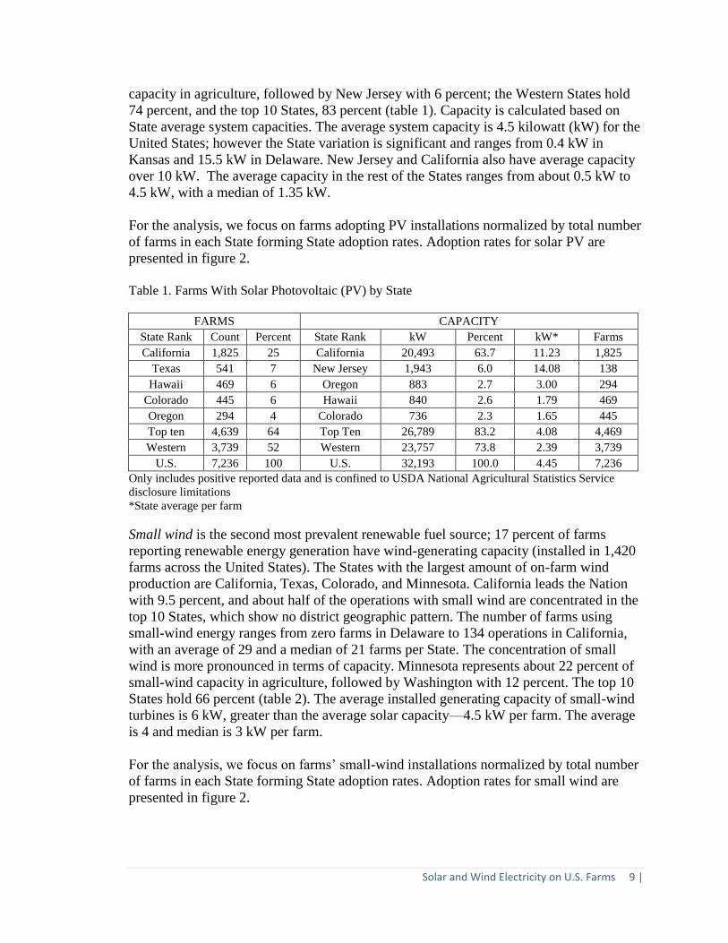
Solar and Wind Electricity on U.S. Farms 9 |
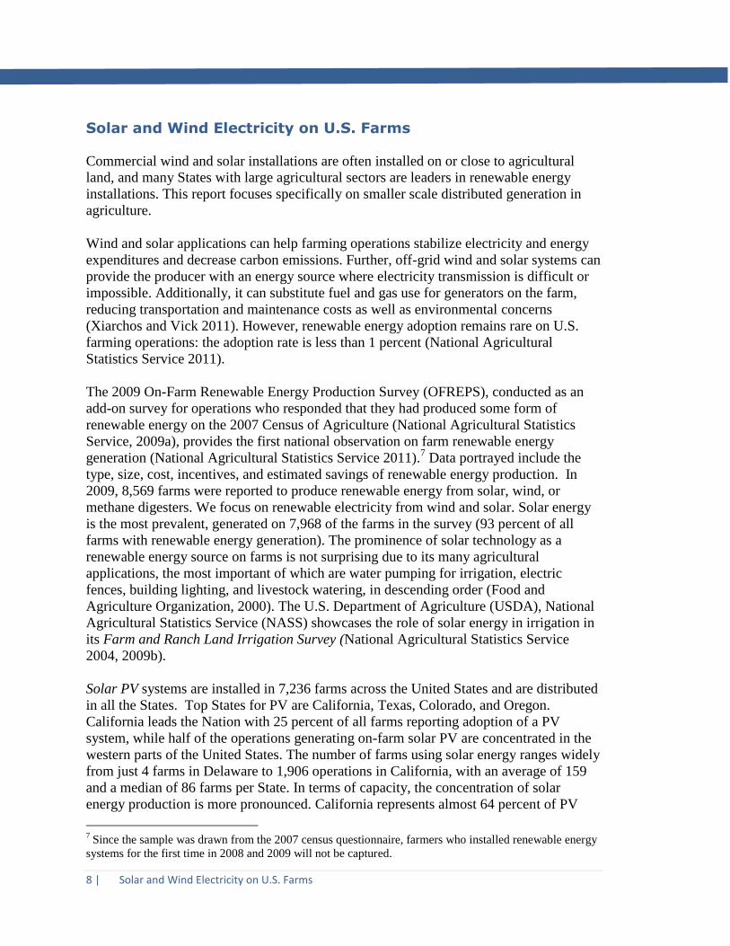
capacity in agriculture, followed by New Jersey with 6 percent; the Western States hold
74 percent, and the top 10 States, 83 percent (table 1). Capacity is calculated based on
State average system capacities. The average system capacity is 4.5 kilowatt (kW) for the
United States; however the State variation is significant and ranges from 0.4 kW in
Kansas and 15.5 kW in Delaware. New Jersey and California also have average capacity
over 10 kW. The average capacity in the rest of the States ranges from about 0.5 kW to
4.5 kW, with a median of 1.35 kW.
For the analysis, we focus on farms adopting PV installations normalized by total number
of farms in each State forming State adoption rates. Adoption rates for solar PV are
presented in figure 2.
Table 1. Farms With Solar Photovoltaic (PV) by State
FARMS CAPACITY
State Rank Count Percent State Rank kW Percent kW* Farms
California 1,825 25 California 20,493 63.7 11.23 1,825
Texas 541 7 New Jersey 1,943 6.0 14.08 138
Hawaii 469 6 Oregon 883 2.7 3.00 294
Colorado 445 6 Hawaii 840 2.6 1.79 469
Oregon 294 4 Colorado 736 2.3 1.65 445
Top ten 4,639 64 Top Ten 26,789 83.2 4.08 4,469
Western 3,739 52 Western 23,757 73.8 2.39 3,739
U.S. 7,236 100 U.S. 32,193 100.0 4.45 7,236
Only includes positive reported data and is confined to USDA National Agricultural Statistics Service
disclosure limitations
*State average per farm
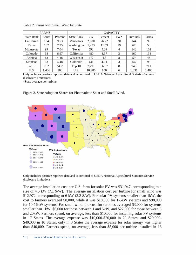
Small wind is the second most prevalent renewable fuel source; 17 percent of farms
reporting renewable energy generation have wind-generating capacity (installed in 1,420
farms across the United States). The States with the largest amount of on-farm wind
production are California, Texas, Colorado, and Minnesota. California leads the Nation
with 9.5 percent, and about half of the operations with small wind are concentrated in the
top 10 States, which show no district geographic pattern. The number of farms using
small-wind energy ranges from zero farms in Delaware to 134 operations in California,
with an average of 29 and a median of 21 farms per State. The concentration of small
wind is more pronounced in terms of capacity. Minnesota represents about 22 percent of
small-wind capacity in agriculture, followed by Washington with 12 percent. The top 10
States hold 66 percent (table 2). The average installed generating capacity of small-wind
turbines is 6 kW, greater than the average solar capacity—4.5 kW per farm. The average
is 4 and median is 3 kW per farm.
For the analysis, we focus on farms’ small-wind installations normalized by total number
of farms in each State forming State adoption rates. Adoption rates for small wind are
presented in figure 2.
10 | Solar and Wind Electricity on U.S. Farms
Table 2. Farms with Small Wind by State
FARMS CAPACITY
State Rank Count Percent State Rank kW Percent kW* Turbines Farms
California 134 9.53 Minnesota 2,880 26.22 20 144 99
Texas 102 7.25 Washington 1,273 11.59 19 67 50
Minnesota 99 7.04 Texas 592 5.39 4 148 102
Colorado 98 6.97 California 480 4.37 3 160 134
Arizona 63 4.48 Wisconsin 472 4.3 8 59 46
Montana 63 4.48 Colorado 441 4.01 3 147 98
Top 10 762 54.2 Top 10 7,291 66.37 8 946 711
U.S. 1,406 100 U.S. 10,986 100 6 1,831 1,406
Only includes positive reported data and is confined to USDA National Agricultural Statistics Service
disclosure limitations
*State average per turbine
Figure 2. State Adoption Shares for Photovoltaic Solar and Small Wind.
Only includes positive reported data and is confined to USDA National Agricultural Statistics Service
disclosure limitations.
The average installation cost per U.S. farm for solar PV was $31,947, corresponding to a
size of 4.5 kW (7.1 $/W). The average installation cost per turbine for small wind was
$12,972, corresponding to 6 kW (2.2 $/W). For solar PV systems smaller than 1kW, the
cost to farmers averaged $8,000, while it was $18,000 for 1-5kW systems and $98,000
for 10-16kW systems. For small wind, the cost for turbines averaged $3,000 for systems
smaller than 1kW, $6,000 for those between 1 and 5kW, and $27,000 for those between 5
and 20kW. Farmers spend, on average, less than $10,000 for installing solar PV systems
in 17 States. The average expense was $10,000-$20,000 in 20 States, and $20,000-
$40,000 in 10 States; only in 3 States the average expense for solar energy was higher
than $40,000. Farmers spend, on average, less than $5,000 per turbine installed in 13

Solar and Wind Electricity on U.S. Farms 11 |
States. The average expense was $5,000-10,000 in 10 States, $10,000-$20,000 in 12
States, and $20,000-$50,000 in 6 States.
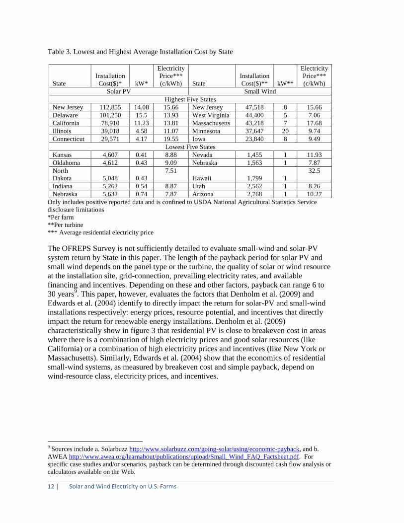
Table 3 shows the States with the highest and lowest installation costs, and the
corresponding average residential electricity prices. There does not seem to be much
correlation between State-level electricity prices and installation costs for small
wind(r=0.02); correlation is more substantial in the case of solar PV (r=0.32). State-level
electricity prices will affect the period of time needed for a farmer to recoup the initial
investment in the renewable system. While the average installation costs are higher in
New Jersey and Delaware relative to Nebraska and Indiana, for example, electricity
prices are also much higher, indicating that over the life of the system, potential savings
could be much higher. The payback period (time to recover initial installation costs) and
potential lifetime savings are two metrics that a farmer may consider in addition to
installation costs when deciding to invest in a renewable system.
Farmers that produced renewable energy on-farm reported savings on their utility bills for
2009 in nearly every State.8 The savings were especially noticeable in New York, with
annual savings over $5,000; Rhode Island and California with annual savings over $4,000;
as well as South Carolina, Vermont, New Jersey, and Arizona with annual savings above
the national average of $2,400. The median utility savings was $1,250; 13 States saved less
than $1,000 in utility bills, 21 between $1,000-2,000, and 15 over $2,000.
The period of time needed for a farmer to recoup the initial investment in the renewable
system will also be influenced by the financial support received. Farmers received
financial support for installing renewable electricity from a number of sources such as
Federal, State, and local government, as well as utilities. The average financial support
received for solar PV was 44 percent of the project cost, slightly lower than the support
for small wind (49 percent).
8 Includes farmers that reported wind turbines, solar panels, and/or methane digesters.
12 | Solar and Wind Electricity on U.S. Farms
Table 3. Lowest and Highest Average Installation Cost by State
State
Installation
Cost($)* kW*
Electricity
Price***
(c/kWh) State
Installation
Cost($)** kW**
Electricity
Price***
(c/kWh)
Solar PV Small Wind
Highest Five States
New Jersey 112,855 14.08 15.66 New Jersey 47,518 8 15.66
Delaware 101,250 15.5 13.93 West Virginia 44,400 5 7.06
California 78,910 11.23 13.81 Massachusetts 43,218 7 17.68
Illinois 39,018 4.58 11.07 Minnesota 37,647 20 9.74
Connecticut 29,571 4.17 19.55 Iowa 23,840 8 9.49
Lowest Five States
Kansas 4,607 0.41 8.88 Nevada 1,455 1 11.93
Oklahoma 4,612 0.43 9.09 Nebraska 1,563 1 7.87
North
Dakota 5,048 0.43
7.51
Hawaii 1,799 1
32.5
Indiana 5,262 0.54 8.87 Utah 2,562 1 8.26
Nebraska 5,632 0.74 7.87 Arizona 2,768 1 10.27
Only includes positive reported data and is confined to USDA National Agricultural Statistics Service
disclosure limitations
*Per farm
**Per turbine
*** Average residential electricity price
The OFREPS Survey is not sufficiently detailed to evaluate small-wind and solar-PV
system return by State in this paper. The length of the payback period for solar PV and
small wind depends on the panel type or the turbine, the quality of solar or wind resource
at the installation site, grid-connection, prevailing electricity rates, and available
financing and incentives. Depending on these and other factors, payback can range 6 to
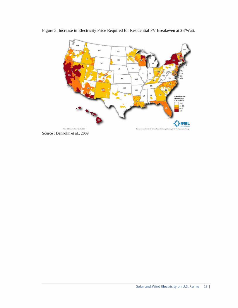
30 years9. This paper, however, evaluates the factors that Denholm et al. (2009) and
Edwards et al. (2004) identify to directly impact the return for solar-PV and small-wind
installations respectively: energy prices, resource potential, and incentives that directly
impact the return for renewable energy installations. Denholm et al. (2009)
characteristically show in figure 3 that residential PV is close to breakeven cost in areas
where there is a combination of high electricity prices and good solar resources (like
California) or a combination of high electricity prices and incentives (like New York or
Massachusetts). Similarly, Edwards et al. (2004) show that the economics of residential
small-wind systems, as measured by breakeven cost and simple payback, depend on
wind-resource class, electricity prices, and incentives.
9 Sources include a. Solarbuzz http://www.solarbuzz.com/going-solar/using/economic-payback, and b.
AWEA http://www.awea.org/learnabout/publications/upload/Small_Wind_FAQ_Factsheet.pdf. For
specific case studies and/or scenarios, payback can be determined through discounted cash flow analysis or
calculators available on the Web.
Solar and Wind Electricity on U.S. Farms 13 |
Figure 3. Increase in Electricity Price Required for Residential PV Breakeven at $8/Watt.
Source : Denholm et al., 2009
14 | Factors Influencing Solar and Wind System Adoption on Farms
Factors Influencing Solar and Wind System Adoption on Farms
A range of potential factors that may account for State variations in renewable electricity
adoption rates on farms is identified and evaluated.10
Descriptive statistics and
correlation analysis are presented.11
Bivariate statistical correlation tests are performed,
and significance is denoted as *** at the 0.01 level, and ** at the 0.05 level and * at the
0.10 level. A multivariate specification is constructed in the next section, following Menz
and Vachon (2006) and Adelaja and Hailu (2008), to account for policy and institutional
influences while controlling for structural and economic factors in the States (Adelaja and
Hailu 2008, Yin and Powers, 2010, Shrimali and Kniefel 2011).12
Even though the rigor
of this analysis is restricted because some of the State characteristics do not necessarily
represent the specific characteristics of the solar adopters, the analysis is pursued in order
to understand adoption at the aggregate State level and to identify policy choices that can
have an impact in renewable electricity technology adoption in the agricultural sector
while accounting for other influences. This paper may also guide further analysis of
farmer adoption behavior at the microdata level and serve as a background for future
interpretations.13
Economic Factors
The influence of economic factors on renewable energy adoption has been examined on
the residential (Mills and Schleich 2009, Fujii and Mak, 1984; Durham et al., 1988) and
State (Adelaja and Hailu 2008) level. We focus on energy prices and resource potential
that directly impact the return for renewable energy installations.
The cost of energy can be an important determinant for the diffusion of solar and wind
energy. The State average electricity and diesel prices (p.electricity and p.diesel)
approximate avoided energy costs when renewable electricity is produced on-farm. The
electricity prices represent prices for residential customers in 2008 (U.S. Energy
Information Administration, 2012a). Diesel prices are computed by subtracting State
taxes from 2008 average regional on-highway (No2) diesel fuel prices (U.S. Energy
Information Administration 2012b; U.S. Energy Information Administration 2009b).
The Pearson’s correlation coefficient for the adoption share of PV (PVAS) is 0.48***
with diesel prices and 0.35** with electricity prices.14
The Pearson’s correlation for the
adoption share of wind (SWAS) is 0.45*** with diesel and 0.35** with electricity prices.
10
Variable abbreviations are summarized in table 13 of the appendix. 11
Descriptive statistics are presented in table 14 of the appendix for select variables. 12
Preliminary correlation analysis provides the basis for variable selection in the multivariate analysis
because of limitations imposed by the small number of observations (Evans and Olson, 2003). 13
Results can guide attention to variables of interest and be compared to future analysis; inferences about
individual adoption impacts, however, are not recommended because of the potential of ecological
inference fallacy (Robinson, 1950). 14
Pearson’s correlation coefficient is a measure of the strength of linear dependence between two variables
that ranges from +1 to -1.
Factors Influencing Solar and Wind System Adoption on Farms 15 |
Solar and wind energy can directly replace electricity for on-grid applications and fossil-
based fuels for off-grid applications. Most of the early adoption of PV on farms was for
off-grid applications like water pumping; however, in the last decade, most PV additions
have been on-grid.
State average electricity and diesel prices are highly correlated (r = 0.73), and
consequently, only one is used in the multivariate analysis. Electricity prices
(p.electricity) vary widely across States, ranging from $6.99/kWh in Idaho and
$19.55/kWh in Connecticut. There is less variation in diesel prices (p.diesel); the
coefficient of variation is 2.8 percent for diesel prices compared to 28.7 percent for
electricity prices. So, it seems likely that even though electricity prices are less closely
correlated with adoption than are diesel fuel prices, the wider variation in electricity
prices makes them a better measure to reflect State-level differences in energy costs.
The economics of a renewable energy installation are also dependent on the resource
potential available for energy production. The more potential there is for energy
production, the faster the payback period is for the initial investment in the renewable
system and the larger potential savings over the life of the system. Therefore, consumers’
adoption behavior might likely be influenced by how “sunny” or “windy” their State is.
We calculate the State resource potential for both wind and solar. The State annual
average for daily solar resource denoted as PV resource was calculated in ArcGIS from
low resolution data (surface cells of approximately 40 km by 40 km in size) developed by
the National Renewable Energy Laboratory’s (NREL’s) Climatological Solar Radiation
Model (National Renewable Energy Laboratory 2009). Arizona has the highest average
State annual solar resource potential at 6.2 kWh/m2/day, and Michigan the lowest at 4.2
kWh/m2/day. The wind resource potential was calculated as an integer from one through
five designating the average State wind classification based on wind-power density at 50
meters. The State averages were calculated in ArcGIS based on low-resolution data (25-
kilometer grid cell resolution) from the national wind-resource assessment of the United
States, first created for the U.S. Department of Energy by the Pacific Northwest
Laboratory (National Renewable Energy Laboratory 2003). Mississippi, with an average
classification of one, has the lowest State average, while Maine, North Dakota, and South
Dakota have the highest, with an average classification of 5. The correlation of the PV-
adoption share is 0.28* with solar resource, while the correlation of the wind-adoption
share with the wind resource of 0.21 is non-significant.
Institutional Factors
The Rural Electrification Act of 1936 led to the formation of numerous cooperatives
tending to rural electrification. As a consequence, farms are often served by electric
cooperatives which are member-owned, private, independent, and non-profit electric
utilities. The percentage of electric customers served by an electric cooperative (% coop)
is included as an indicator of the prevalence of cooperatives in the electricity generation
for each State, based on data available from the U.S. Energy Information Administration
(U.S. Energy Information Administration 2012c). Electric cooperatives have distinct
characteristics that can impact renewable energy adoption by farms. For example, the
16 | Factors Influencing Solar and Wind System Adoption on Farms
high cost of maintaining the infrastructure needed to cover large rural areas can cause
prices for electric cooperatives to be higher. Indicatively, in Kentucky, electric
cooperatives serve an average of eight consumers per mile of electric line, while investor-
owned utilities (IOU) and municipal utilities serve 25 and 60 consumers per mile of
electric line respectively (KAEC). Additionally, electric cooperatives, unlike IOUs, are
not required by the Public Utility Regulatory Policies Act of 1978 (PURPA) to
interconnect with and purchase power at avoided cost from customers with excess onsite
generation. Similarly, many States with net metering, interconnection, and RPS exclude
cooperatives from the regulation. Not surprisingly, the adoption share on farms is
negatively correlated with the share of customers in the State that purchase electricity
from electric cooperatives (r=-0.35** for PV adoption and r=-0.28* for wind adoption).
Policy Factors
Renewable energy policies have been important to the growth of renewable electricity
production in the last decade. However, policies promoting renewable electricity
development vary widely from State to State in formulation and effectiveness. Menz and
Vachon (2006), Adelaja and Hailu (2008), Yin and Powers (2010), and Shrimali and
Kniefel (2011) examined policies expected to impact State-level adoption at the utility-
scale. Our examination is unique as it focuses on policies that can impact State-level
adoption of distributed generation specifically in agriculture. Table 4 shows Pearson’s
correlation for the different policy instruments promoting distributed generation with
solar PV and small-wind adoption rates in agriculture. Table 8 provides a view of the
geographic distribution of such State policies.
RPS
Renewable Portfolio Standards (RPS) require a minimum amount of renewable electricity
sales, or generating capacity, that electricity utilities must achieve according to a
specified schedule of dates and mandates. By December 2009, 29 States and the District
of Columbia had established an RPS.15
The specified target amount and date to meet the
requirements varied by State. Some States also provided specific solar and/or distributed
generation (DG) “set asides.” A “set-aside,” also called a “carve-out,” is a provision
within an RPS that requires utilities to use a specific renewable resource to meet a certain
percentage of their RPS. While RPS policies are designed to encourage utility-scale
investments, those set-aside provisions provide incentives specifically for DG, such as
solar and small-wind. Sixteen States and the District of Columbia have such set-asides
implemented (Database of State Incentives for Renewables & Efficiency, DSIRE).
The RPS variables presented in the study are based on our analysis of DSIRE's
Quantitative RPS Data Project (2009) for December 2009. RPS targets represent a
percentage of retail electricity sales covered by the RPS at the final target date in each
State. We estimate the RPS target for new renewable generation (nr rps target) by
excluding traditional sources like biomass and hydro from our interpretation of the RPS
tiers for each State. Similarly, we identify solar and distributed generation RPS set-aside
15
Two States express their target in terms of installed capacity, while five additional States set a non-
binding renewable energy goal. Those are excluded from the analysis.
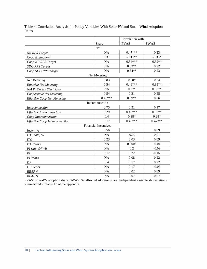
Factors Influencing Solar and Wind System Adoption on Farms 17 |
targets (sdg rps target). We further identify States that exempt cooperatives from the RPS
(coop exemption) and States that have a separate RPS for cooperatives (coop _ rps) as
well as the respective targets that the cooperatives face (coop rps target). New renewable
RPS targets (nr rps target) vary from zero to 33 percent of electricity sales, while
solar/DG RPS targets (sdg rps target) only reach 5 percent. When a separate target is
granted to cooperatives, it is much lower. Correlations with the different RPS indices are
large and significant for solar adoption rates (maximum of 0.54 for coop new RPS
target); they are much smaller for small-wind adoption rates and only significant for coop
new RPS target and coop exemption. As expected, the adoption rates are negatively
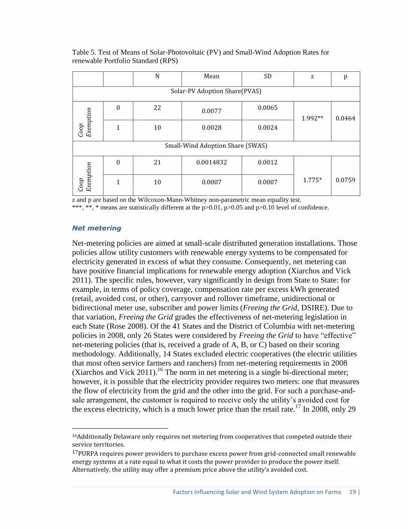
correlated with coop exemptions. We also find that there is a statistically significant
difference in the mean adoption rate of States with a coop exemption relative to those
without one (table 5). The overall and cooperative specific targets are highly correlated
both for new renewables (r=0.79) and solar/DG(r=99), and only one of each is used in the
analysis.
18 | Factors Influencing Solar and Wind System Adoption on Farms
Table 4. Correlation Analysis for Policy Variables With Solar-PV and Small Wind Adoption
Rates
Correlation with
Share PVAS SWAS
RPS
NR RPS Target NA 0.47*** 0.23
Coop Exemption 0.31 -0.39** -0.35*
Coop NR RPS Target NA 0.54*** 0.32**
SDG RPS Target NA 0.33** 0.22
Coop SDG RPS Target NA 0.34** 0.23
Net Metering
Net Metering 0.83 0.28* 0.24
Effective Net Metering 0.54 0.46*** 0.35**
NM P. Excess Electricity NA 0.27* 0.30**
Cooperative Net Metering 0.54 0.21 0.25
Effective Coop Net Metering 0.40*** 0.39** 0.36
Interconnection
Interconnection 0.75 0.21 0.17
Effective Interconnection 0.29 0.47*** 0.37**
Coop Interconnection 0.4 0.28* 0.28*
Effective Coop Interconnection 0.17 0.43*** 0.47***
Financial Incentives
Incentive 0.56 0.1 0.09
ITC rate, % NA -0.02 0.01
ITC 0.23 0.03 0.09
ITC Years NA 0.0008 -0.04
PI rate, $/kWh NA 0.2 -0.09
PI 0.17 0.22 -0.07
PI Years NA 0.08 0.22
DP 0.4 0.17 0.22
DP Years NA 0.17 -0.06
REAP # NA 0.02 0.09
REAP $ NA 0.07 0.07
PVAS: Solar-PV adoption share. SWAS: Small-wind adoption share. Independent variable abbreviations
summarized in Table 13 of the appendix.
Factors Influencing Solar and Wind System Adoption on Farms 19 |
Table 5. Test of Means of Solar-Photovoltaic (PV) and Small-Wind Adoption Rates for
renewable Portfolio Standard (RPS)
N Mean SD z p
Solar-PV Adoption Share(PVAS)
Co
op
E
xem
pti
on
0 22 0.0077 0.0065
1.992** 0.0464
1 10 0.0028 0.0024
Small-Wind Adoption Share (SWAS)
Co
op
E
xem
pti
on
0 21 0.0014832 0.0012
1.775*
0.0759 1 10 0.0007 0.0007
z and p are based on the Wilcoxon-Mann-Whitney non-parametric mean equality test.
***, **, * means are statistically different at the p>0.01, p>0.05 and p>0.10 level of confidence.
Net metering
Net-metering policies are aimed at small-scale distributed generation installations. Those
policies allow utility customers with renewable energy systems to be compensated for
electricity generated in excess of what they consume. Consequently, net metering can
have positive financial implications for renewable energy adoption (Xiarchos and Vick
2011). The specific rules, however, vary significantly in design from State to State: for
example, in terms of policy coverage, compensation rate per excess kWh generated
(retail, avoided cost, or other), carryover and rollover timeframe, unidirectional or
bidirectional meter use, subscriber and power limits (Freeing the Grid, DSIRE). Due to
that variation, Freeing the Grid grades the effectiveness of net-metering legislation in
each State (Rose 2008). Of the 41 States and the District of Columbia with net-metering
policies in 2008, only 26 States were considered by Freeing the Grid to have “effective”
net-metering policies (that is, received a grade of A, B, or C) based on their scoring
methodology. Additionally, 14 States excluded electric cooperatives (the electric utilities
that most often service farmers and ranchers) from net-metering requirements in 2008
(Xiarchos and Vick 2011).16
The norm in net metering is a single bi-directional meter;
however, it is possible that the electricity provider requires two meters: one that measures
the flow of electricity from the grid and the other into the grid. For such a purchase-and-
sale arrangement, the customer is required to receive only the utility’s avoided cost for
the excess electricity, which is a much lower price than the retail rate.17
In 2008, only 29
16Additionally Delaware only requires net metering from cooperatives that competed outside their service territories. 17PURPA requires power providers to purchase excess power from grid-connected small renewable energy systems at a rate equal to what it costs the power provider to produce the power itself. Alternatively, the utility may offer a premium price above the utility’s avoided cost.
20 | Factors Influencing Solar and Wind System Adoption on Farms
States and the District of Columbia offered retail electricity price for the excess
electricity generated.
According to the U.S. Energy Information Administration (2009a, 2010, 2011), the
number of renewable electricity customers in net-metering programs has been steadily
increasing: from 4,472 customers in 2002 to 48,886 customers in 2007, up to 96,506
customers in 2009. The majority of those customers (over 90 percent) are residential.18
Five indicators for net metering are examined: having a net metering regulation, having
an effective net metering regulation, and having the regulation apply to electric
cooperatives in the State (coop net metering and coop effective net metering) as well as
the excess electricity price received in each State based on the net-metering rules (nm p.
excess electricity). Net-metering indicators have lower correlations than effective net-
metering indicators. Low correlation is also found for the estimate of the price received
for excess electricity based on the net-metering rules of each State. Correlation is highest
for effective net metering (r=0.46) and effective coop net metering (r=0.39). Focusing on
those net metering indicators, we find that there is a statistically significant difference in
the mean adoption rate of States with effective net-metering rules relative to those
without effective net-metering rules for PV adoption (table 6). The statistical significance
is highest for effective net metering. For effective cooperative net metering, Wilcoxon’s
rank-sum test of means is statistically significant only at the p>0.10 level of confidence,
while for small wind, Wilcoxon’s rank-sum test of means for adoption rates is
statistically significant only for effective net metering at the 10-percent significance level.
Another observation is that the correlation for cooperative indicators does not differ
substantially from the respective general State indicators.19
Due to the high correlation of
the cooperative and the general State effective net-metering indicators (r=0.74), only the
general State effective net metering is evaluated in the multivariate analysis.
18
Some farms are included in the Energy Information Administration (EIA) “residential” category, while
other farms are classified as commercial customers depending on the utility schedule they qualify for. 19
Wilcoxon’s rank-sum test of means for States with (effective) interconnection by (effective) coop
interconnection further supports that the mean adoption rates of States with (effective) net metering does
not differ significantly for States that exclude electric cooperatives from the regulation (not shown but
available upon request).
Factors Influencing Solar and Wind System Adoption on Farms 21 |
Table 6. Test of Means of Solar-Photovoltaic (PV) and Small-Wind Adoption Rates for Net
Metering
N Mean SD z p
Solar-PV Adoption Share(PVAS)
Eff
ecti
ve
Net
Met
erin
g 0 22 0.0024 0.0025
-2.607***
0.0091 1 26 0.0077 0.0067
Eff
ecti
ve
Co
op
Net
Met
erin
g 0 34 0.0035 0.0042
-1.929*
0.0537 1 14 0.0094 0.0071
Small-Wind Adoption Share(SWAS)
Eff
ecti
ve
Net
Met
erin
g 0 21 0.0005806 0.0006
-1.819*
0.0689 1 25 0.0015 0.0016
Eff
ecti
ve
Co
op
Net
Met
erin
g 0 28 0.0007 0.0007
-1.418
0.1562 1 18 0.0016 0.0018
z and p are based on the Wilcoxon-Mann-Whitney non-parametric mean equality test.
***, **, * means are statistically different at the p>0.01, p>0.05 and p>0.10 level of confidence.
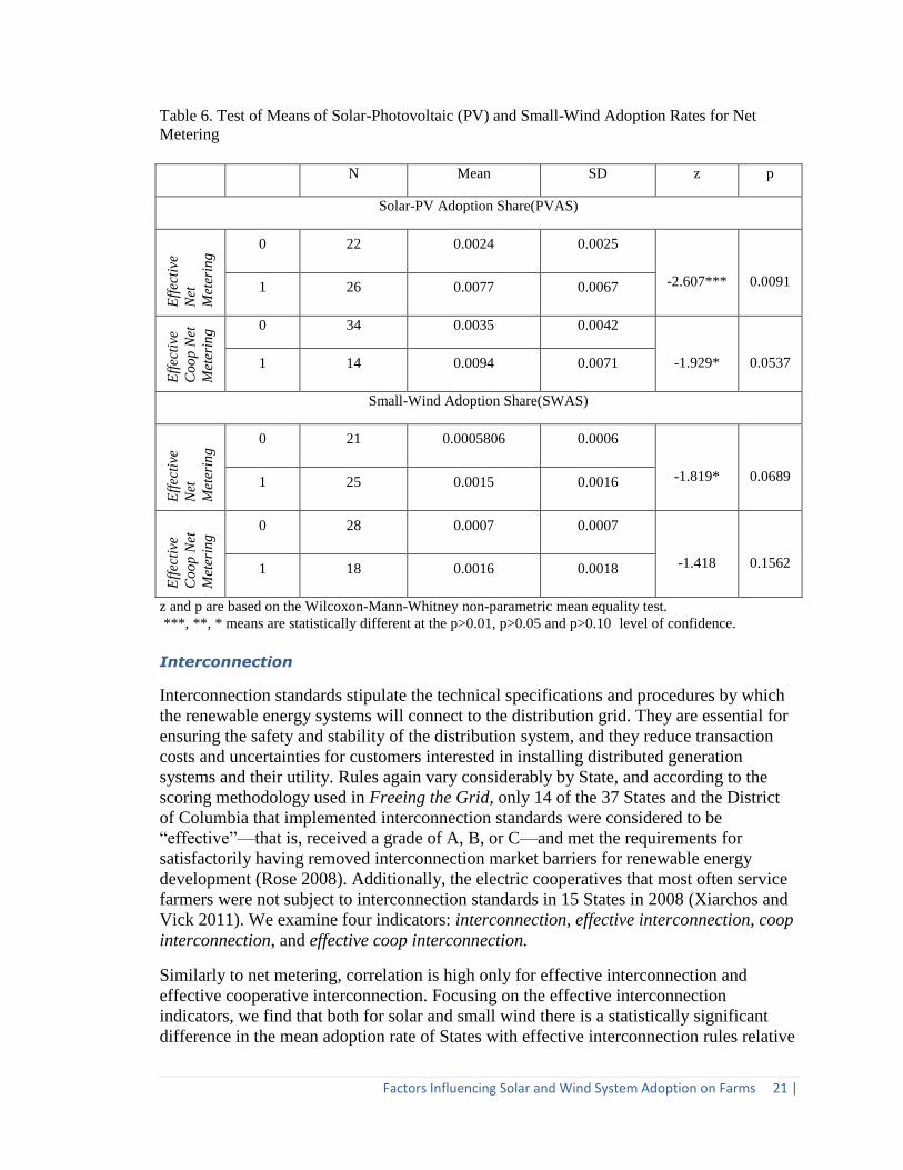
Interconnection
Interconnection standards stipulate the technical specifications and procedures by which
the renewable energy systems will connect to the distribution grid. They are essential for
ensuring the safety and stability of the distribution system, and they reduce transaction
costs and uncertainties for customers interested in installing distributed generation
systems and their utility. Rules again vary considerably by State, and according to the
scoring methodology used in Freeing the Grid, only 14 of the 37 States and the District
of Columbia that implemented interconnection standards were considered to be
“effective”—that is, received a grade of A, B, or C—and met the requirements for
satisfactorily having removed interconnection market barriers for renewable energy
development (Rose 2008). Additionally, the electric cooperatives that most often service
farmers were not subject to interconnection standards in 15 States in 2008 (Xiarchos and
Vick 2011). We examine four indicators: interconnection, effective interconnection, coop
interconnection, and effective coop interconnection.
Similarly to net metering, correlation is high only for effective interconnection and
effective cooperative interconnection. Focusing on the effective interconnection
indicators, we find that both for solar and small wind there is a statistically significant
difference in the mean adoption rate of States with effective interconnection rules relative
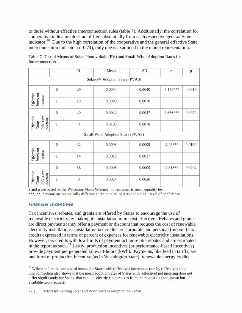
22 | Factors Influencing Solar and Wind System Adoption on Farms
to those without effective interconnection rules (table 7). Additionally, the correlation for
cooperative indicators does not differ substantially from each respective general State
indicator.20
Due to the high correlation of the cooperative and the general effective State
interconnection indicator (r=0.74), only one is examined in the model representation.
Table 7. Test of Means of Solar-Photovoltaic (PV) and Small-Wind Adoption Rates for
Interconnection
N Mean SD z p
Solar-PV Adoption Share (PVAS)
Eff
ecti
ve
Inte
rco
n-
nec
tio
n
0 29 0.0034 0.0040 -3.153*** 0.0016
1 19 0.0080 0.0070
Eff
ecti
ve
Co
op
Inte
rco
n-
nec
tio
n
0 40 0.0042 0.0047 -2.656*** 0.0079
1 8 0.0108 0.0078
Small-Wind Adoption Share (SWAS)
Eff
ecti
ve
Inte
rco
n-
nec
tio
n
0 32 0.0008 0.0009 -2.483** 0.0130
1 14 0.0018 0.0017
Eff
ecti
ve
Co
op
Inte
rco
n-
nec
tio
n
0 38 0.0008 0.0009 -2.318** 0.0204
1 8 0.0024 0.0020
z and p are based on the Wilcoxon-Mann-Whitney non-parametric mean equality test.
***, **, * means are statistically different at the p>0.01, p>0.05 and p>0.10 level of confidence.
Financial Incentives
Tax incentives, rebates, and grants are offered by States to encourage the use of
renewable electricity by making its installation more cost effective. Rebates and grants
are direct payments: they offer a payment or discount that reduces the cost of renewable
electricity installations. Installation tax credits are corporate and personal (income) tax
credits expressed in terms of percent of expenses for renewable electricity installations.
However, tax credits with low limits of payment act more like rebates and are estimated
in the report as such.21
Lastly, production incentives (or performance-based incentives)
provide payment per generated kilowatt-hours (kWh). Payments, like feed in tariffs, are
one form of production incentive (as in Washington State); renewable energy credits
20
Wilcoxon’s rank-sum test of means for States with (effective) interconnection by (effective) coop
interconnection also shows that the mean adoption rates of States with (effective) net metering does not
differ significantly for States that exclude electric cooperatives from the regulation (not shown but
available upon request).
Factors Influencing Solar and Wind System Adoption on Farms 23 |
(RECs) and solar RECs (SRECs) are another (examples include California and
Pennsylvania). Even a tax credit can be a performance-based incentive, like in Nebraska,
where the tax credit offered is based on generated kWhs.
Twenty-seven States were identified to have some State incentive (incentive) that
supported small-scale renewable distributed generation in 2008: 11 had tax credits (ITC);
19 had grant and rebate programs (DP); and 8 had production incentives (PI). Loan
programs can also provide financing for the purchase of renewable energy equipment, but
such programs are not identified for our analysis. Database of State Incentives for
Renewables and Efficiency (DSIRE), individual State programs, and REC markets were
consulted to extract the financial variables examined. We include policy dummy
variables and, when quantitatively comparable, we also include the incentive rates as well
as the years since the policy adoption as measures of policy stringency. A binary variable
is included for having some incentive (incentive) and for each policy separately: ITC, PI,
and DP. For the investment tax credit and the production incentive, we also have each
State’s rate (ITC rate and PI rate) and the years from adoption (ITC years and PI years).
For direct payments, incentives are not easily compatible, so we only include the years
since policy adoption (DP years). We find that correlations with renewable electricity
adoption rates are small and insignificant, not only for the binary variables but also for
the incentive rates and years since enactment, which are examined as measures of policy
stringency. The results are somewhat surprising provided the high upfront capital cost of
renewable energy installations and the potential for those policies to increase cost
effectiveness.
Rural Development’s Renewable Energy Systems and Energy Efficiency Improvement
Program, renamed Rural Energy for America (REAP) in the 2008 Farm Bill, has also
provided some financial support to solar and small-wind installations. Most of the
awards, however, have been for energy efficiency; for example, 74 percent in 2008. From
2001 to 2009, USDA’s Rural Development funded 550 solar and small-wind projects
with a total of over $17.5 million in funds. However, through 2009, awards were
geographically concentrated to only a few States and did not focus on smaller systems
(Xiarchos and Vick 2011). Consequently, State adoption rates for solar and small-wind
are not expected to be highly correlated with the number of REAP awards in the State
(REAP #), or the dollar amount of awards (REAP $). Program changes after 2009 should
make them a more influential factor (Xiarchos and Vick 2011), provided continuation of
program funding in the coming years.
21
For the purposes of this study, we placed tax credits with a limit of $2,000 or less in the “rebates”
category. Tax credits with a limit of more than $2,000 are shown in the “tax credits” category.
24 | Factors Influencing Solar and Wind System Adoption on Farms
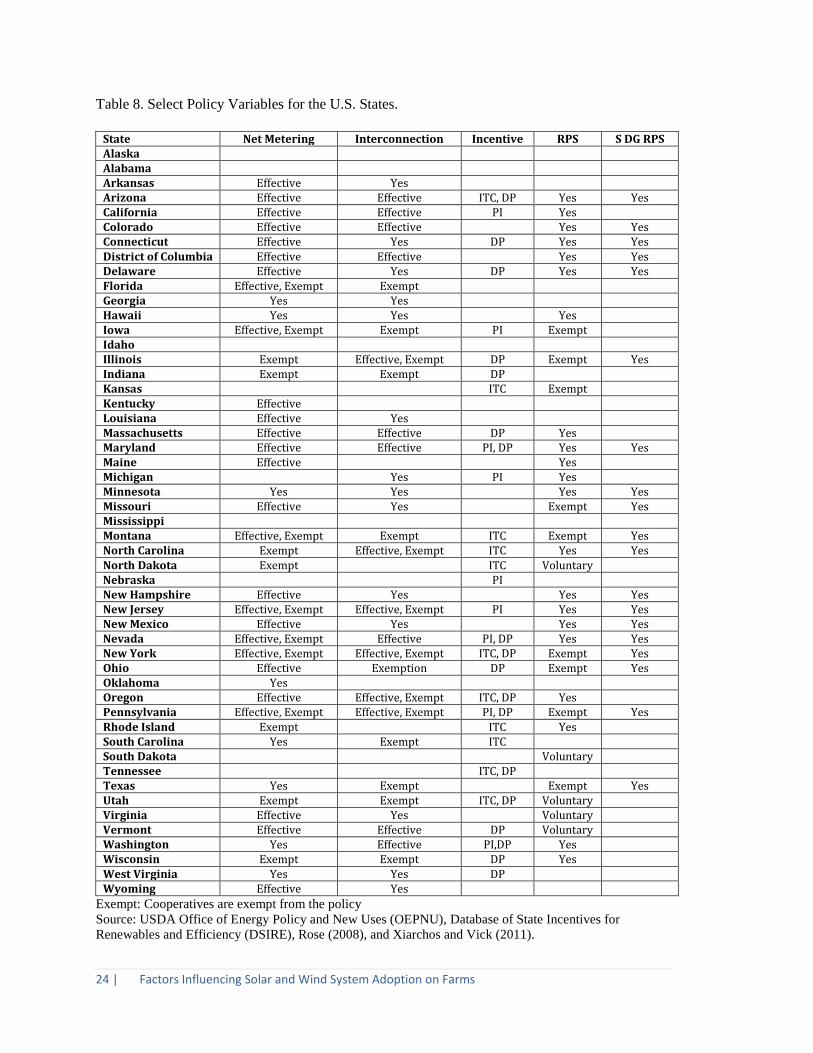
Table 8. Select Policy Variables for the U.S. States.
State Net Metering Interconnection Incentive RPS S DG RPS Alaska
Alabama
Arkansas Effective Yes
Arizona Effective Effective ITC, DP Yes Yes California Effective Effective PI Yes
Colorado Effective Effective
Yes Yes
Connecticut Effective Yes DP Yes Yes District of Columbia Effective Effective
Yes Yes
Delaware Effective Yes DP Yes Yes Florida Effective, Exempt Exempt
Georgia Yes Yes
Hawaii Yes Yes
Yes
Iowa Effective, Exempt Exempt PI Exempt
Idaho
Illinois Exempt Effective, Exempt DP Exempt Yes Indiana Exempt Exempt DP
Kansas
ITC Exempt
Kentucky Effective
Louisiana Effective Yes
Massachusetts Effective Effective DP Yes
Maryland Effective Effective PI, DP Yes Yes Maine Effective
Yes
Michigan
Yes PI Yes
Minnesota Yes Yes
Yes Yes
Missouri Effective Yes
Exempt Yes Mississippi
Montana Effective, Exempt Exempt ITC Exempt Yes North Carolina Exempt Effective, Exempt ITC Yes Yes North Dakota Exempt
ITC Voluntary
Nebraska
PI
New Hampshire Effective Yes
Yes Yes
New Jersey Effective, Exempt Effective, Exempt PI Yes Yes New Mexico Effective Yes
Yes Yes
Nevada Effective, Exempt Effective PI, DP Yes Yes New York Effective, Exempt Effective, Exempt ITC, DP Exempt Yes Ohio Effective Exemption DP Exempt Yes Oklahoma Yes
Oregon Effective Effective, Exempt ITC, DP Yes
Pennsylvania Effective, Exempt Effective, Exempt PI, DP Exempt Yes Rhode Island Exempt
ITC Yes
South Carolina Yes Exempt ITC
South Dakota
Voluntary
Tennessee
ITC, DP
Texas Yes Exempt
Exempt Yes
Utah Exempt Exempt ITC, DP Voluntary
Virginia Effective Yes
Voluntary
Vermont Effective Effective DP Voluntary
Washington Yes Effective PI,DP Yes
Wisconsin Exempt Exempt DP Yes
West Virginia Yes Yes DP
Wyoming Effective Yes
Exempt: Cooperatives are exempt from the policy
Source: USDA Office of Energy Policy and New Uses (OEPNU), Database of State Incentives for
Renewables and Efficiency (DSIRE), Rose (2008), and Xiarchos and Vick (2011).
Factors Influencing Solar and Wind System Adoption on Farms 25 |
State Agricultural Characteristics
Adelaja and Hailu 2008, Yin and Powers 2010, and Shrimali and Kniefel 2011 account
for economic, political, and demographic characteristics. Our analysis focuses in
agriculture, so in addition to such characteristics, we also account for differences in the
agricultural sector of the States. Structural characteristics of the agricultural sector
should have an effect in the resulting renewable electricity adoption rates at the State
level. In this section, we investigate which structural characteristics of the agricultural
sector to include in the multivariate analysis as control variables. Even though most of
the variables can serve as proxies to individual farmer characteristics at the aggregate
level, they are analyzed for representing State conditions that increase the adoption
probability for all farmers in the State. For example, organic acres can indicate a
predisposition in the State’s agricultural sector for addressing environmental concerns.
Another example is share of cattle operations; since a predominant use of renewable
energy systems in agriculture has historically been for water pumping, “ranching” States
with many cattle operations can be expected to have larger adoption rates. All variables
are normalized (as averages by operation or shares in the agricultural sector of the State)
and are extracted from the 2007 Census of Agriculture (National Agricultural Statistics
Service 2009a).
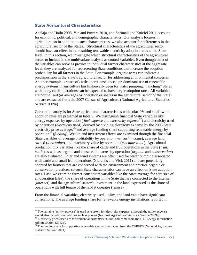
Correlation analysis for State agricultural characteristics with solar-PV and small-wind
adoption rates are presented in table 9. We distinguish financial State variables like
energy expenses by operation ( fuel expense and electricity expense22
) and electricity used
by operation (electricity used), derived by dividing electricity expense by the 2008 State
electricity price average,23
and average funding share supporting renewable energy by
operation24
(funding). Wealth and investment effects are examined through the financial
State variables of average profitability by operation (net cash income), average land
owned (land value), and machinery value by operation (machine value). Agricultural
production mix variables like the share of cattle and fruit operations in the State (fruit,
cattle) as well as organic and conservation acres by operation (organic and conservation)
are also evaluated. Solar and wind systems are often used for water pumping associated
with cattle and small fruit operations (Xiarchos and Vick 2011) and are potentially
adopted by farmers that are concerned with the environment and practice organic or
conservation practices, so such State characteristics can have an effect on State adoption
rates. Last, we examine farmer constituent variables like the State average for acre size of
an operation (size), the share of operations in the State that are connected to the Internet
(internet), and the agricultural sector’s investment in the land expressed as the share of
operations with full tenure of the land it operates (tenure).
From the financial variables, electricity used, utility, and land value have significant
correlations. The average funding share for renewable energy installations reported in
22
The variable “utility expense” is used as a proxy for electricity expense, although the utility expense
would also include other utilities such as phones (National Agricultural Statistics Service 2009a). 23
Electricity prices used are for residential customers in 2008 and come from the U.S. Energy Information
Administration (2012a). 24
The funding share for supporting renewable energy is extracted from the OFREPS (National Agricultural
Statistics Service 2011).
26 | Factors Influencing Solar and Wind System Adoption on Farms
NASS is not correlated with adoption share; this result is in line with the insignificant
correlation for financial policy instruments. Average farm income (representing wealth
and profitability in the State’s agricultural sector), and machine value (representing
wealth as well as capital investment in the State’s agricultural sector) are not correlated
with adoption shares. Average land value, another indicator for wealth, holds a
significant correlation to solar-adoption shares, but not to wind-adoption shares. Fuel
costs are uncorrelated, while electricity cost and electricity use are highly correlated with
adoption rates. Electricity cost and electricity use are highly correlated (r = 0.92) and
consequently only one is used in the multivariate analysis.
The product mix also seems significant. States with a lot of organic production are
significantly correlated with solar and wind adoption rates. The share of cattle operations
in the State is significantly correlated with wind adoption rates, while the share of fruit
operations holds a significant relationship specifically with solar adoption rates. Internet
connection share has a significant correlation with adoption shares, and tenure share has a
significant correlation with the solar PV adoption share. Wind adoption rates are
correlated with less variables (only about half) than solar adoption rates.
Table 9. Correlation Analysis for State Agricultural Characteristics With Solar-PV and Small-
Wind Adoption Rates
PVAS: Solar-PV adoption share. SWAS: Small-wind adoption share.
Independent variable abbreviations summarized in Table 13 of the appendix.
PVAS SWAS
Financial
Fuel Expense 0.23 0.06
Electricity Expense 0.62*** 0.3**
Electricity Used 0.48*** 0.23
Land Value 0.36*** 0.1
Machine Value -0.13 -0.11
Net Cash Income -0.02 -0.11
Funding Share -0.01 -0.09
Product Mix
Conservation Acres 0.02 0.03
Organic Acres 0.6*** 0.68***
Fruit 0.55*** 0.21
Cattle -0.23 -0.33**
Constituent
Internet -0.33** -0.38***
Tenure 0.41*** 0.23
Size 0.22 0.09
Modeling Aggregate Renewable Electricity Adoption 27 |
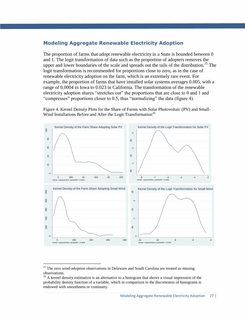
Modeling Aggregate Renewable Electricity Adoption
The proportion of farms that adopt renewable electricity in a State is bounded between 0
and 1. The logit transformation of data such as the proportion of adopters removes the
upper and lower boundaries of the scale and spreads out the tails of the distribution.25
The
logit transformation is recommended for proportions close to zero, as in the case of
renewable electricity adoption on the farm, which is an extremely rare event. For
example, the proportion of farms that have installed solar systems averages 0.005, with a
range of 0.0004 in Iowa to 0.023 in California. The transformation of the renewable
electricity adoption shares “stretches out” the proportions that are close to 0 and 1 and
“compresses” proportions closer to 0.5, thus “normalizing” the data (figure 4).
Figure 4. Kernel Density Plots for the Share of Farms with Solar Photovoltaic (PV) and Small-
Wind Installations Before and After the Logit Transformation26
25
The zero wind-adoption observations in Delaware and South Carolina are treated as missing
observations. 26
A kernel density estimation is an alternative to a histogram that shows a visual impression of the
probability density function of a variable, which in comparison to the discreteness of histograms is
endowed with smoothness or continuity.
02
04
06
08
01
00
Den
sity
0 .005 .01 .015 .02 .025
kernel = epanechnikov, bandwidth = 0.0023
Kernel Density of the Farm Share Adopting Solar PV
.05
.1.1
5.2
.25
.3
Den
sity
-8 -7 -6 -5 -4 -3kernel = epanechnikov, bandwidth = 0.4906
Kernel Density of the Logit Transformation for Solar PV
0
100
200
300
400
500
Den
sity
0 .002 .004 .006 .008kernel = epanechnikov, bandwidth = 0.0005
Kernel Density of the Farm Share Adopting Small Wind
0
.05
.1.1
5.2
.25
Den
sity
-12 -10 -8 -6 -4kernel = epanechnikov, bandwidth = 0.5792
Kernel Density of the Logit Transformation for Small Wind
28 | Modeling Aggregate Renewable Electricity Adoption
The model becomes:
(
)
Aitchison (1986) calls the above transformation the additive logratio transformation and
shows that z will follow a normal distribution, N(μ, σ2), if y follows an additive logistic
normal distribution. Aitchison (1986) proposes testing the appropriateness of the model
(if y is distributed as an additive logistic normal distribution) by testing if z is normally
distributed.
The model is fitted with ordinary least squares (OLS), and its formulation is influenced
from the technology adoption literature. Due to the small number of observations, the
empirical analysis needs to be parsimonious (Evans and Olson, 2003): the determinants
are selected based on the preliminary correlation analysis in the previous section and a
stepwise regression procedure. Results are presented in Table 10 and 11. Model 1
includes factors of interest, while Model 2 includes only those factors that are found to be
significant. The variance inflation factors (VIFs) suggest that multicollinearity does not
pose a problem. The model residuals are normally distributed as supported by the
Shapiro-Wilk, Shapiro-Francia, and Skewness/Kurtosis tests in table 12 at the 1-percent
marginal significance level. Consequently, our data support the distributional
assumptions underlying the logit transformation regression model. We use robust
standard errors, which Kieschnick and McCullough (2003) identify are more trustworthy
for inferring significance with the logit transformation model. The logic transformation is
worth exploring according to Smithson and Verkuilen (2006); it serves our rare event
analysis well, while our data support that modeling approach. However, due to increased
support for using the beta distribution for proportions (Kieschnick and McCullough 2003,
Smithson and Verkuilen (2006), we also run the beta regression and show its results in
tables 10 and 11. The beta regression assumes the dependent variable follows a beta
distribution with two parameters μ and φ:
>0
where
;
The parameters ω and τ are shape parameters (ω pulls the density towards 0 and and τ
toward 1), that are parameterized into a location (mean) μ and a precision φ parameter.
The parameter φ represents dispersion because variance increases as φ decreases: σ=
μ(1- μ)/ φ+1. However, φ is not the sole determinant of dispersion; variance is a function
of both the mean and parameter φ, since the dispersion of a bounded random variable
depends partially on location. Still, the location parameter μ and the precision parameter
φ place no restrictions on each other and can be modeled separately (Smithson and
Verkuilen, 2006). We run the beta regression on the formulation of variables appointed
from the stepwise logit transformation model, and in accordance to Smithson and
Verkuilen (2006), examine impacts of the variables both on the location (μ) and the
dispersion (φ)27
of adoption rates. Explicitly modeling dispersion on explanatory
variables increases the Chi-square for both solar and wind adoption rates. The variables
in the dispersion submodel that maximize the Chi-square are land value for solar
27
The precision factor expressing variance.

Modeling Aggregate Renewable Electricity Adoption 29 |
adoption rates and land value and tenure for wind adoption rates. Slight differences in
the mean results are noted. The beta models pick up significance for some additional
variables to those found significant by the logic transformation regression.
PV adoption rates are positively influenced by economic factors in the State. Higher
electricity prices correspond to higher State adoption rates. Furthermore, solar potential
also accounts for variation in PV adoption rates. Higher radiation is positively related to
increased State-level adoption. Institutional influences also systematically account for
adoption variation. The percentage of State electric customers served by an electric
cooperative is negatively related to PV adoption rates. In terms of policies supporting
renewable electricity, only the solar and distributed generation target has a significant
effect on adoption rates. Correlation analysis already showed a lack of connection
between financial policy instruments and adoption rates, regression analysis further
shows no statistically significant relationship for net-metering and interconnection
policies with State-level adoption shares. Land ownership, Internet connectivity, and
organic practices in agriculture at the State level are also found to have a significant
relationship to adoption rates. The beta regression also picks up a negative relationship
between adoption rates and electricity used in the farm sector.
The picture is similar for small-wind adoption rates. Share of customers served by
electric cooperatives, organic practices, and Internet connectivity in the State have a
systematic link to adoption shares for small wind, while net-metering and interconnection
policies do not. The beta regression further shows a significant systematic positive
relationship with electricity prices. However, some differences arise: adoption rates are
not related to the intensity of the wind resource at the State level or land ownership; the
beta regression also picks up that small-wind adoption rates are systematically related to
the RPS for new renewables in addition to the solar and distributed generation target.
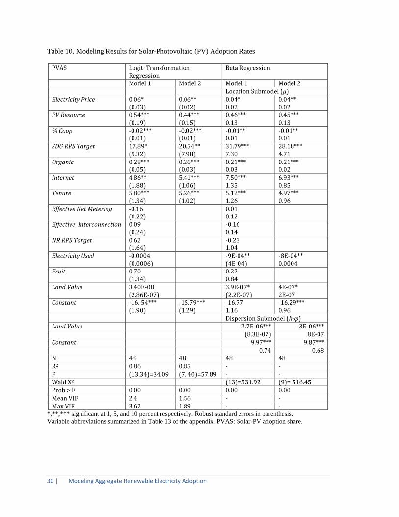
30 | Modeling Aggregate Renewable Electricity Adoption
Table 10. Modeling Results for Solar-Photovoltaic (PV) Adoption Rates
PVAS Logit Transformation Regression
Beta Regression
Model 1 Model 2 Model 1 Model 2 Location Submodel (μ) Electricity Price 0.06* 0.06** 0.04* 0.04** (0.03) (0.02) 0.02 0.02 PV Resource 0.54*** 0.44*** 0.46*** 0.45*** (0.19) (0.15) 0.13 0.13 % Coop -0.02*** -0.02*** -0.01** -0.01** (0.01) (0.01) 0.01 0.01 SDG RPS Target 17.89* 20.54** 31.79*** 28.18*** (9.32) (7.98) 7.30 4.71 Organic 0.28*** 0.26*** 0.21*** 0.21*** (0.05) (0.03) 0.03 0.02 Internet 4.86** 5.41*** 7.50*** 6.93*** (1.88) (1.06) 1.35 0.85 Tenure 5.80*** 5.26*** 5.12*** 4.97*** (1.34) (1.02) 1.26 0.96 Effective Net Metering -0.16 0.01 (0.22) 0.12 Effective Interconnection 0.09 -0.16 (0.24) 0.14 NR RPS Target 0.62 -0.23 (1.64) 1.04 Electricity Used -0.0004 -9E-04** -8E-04** (0.0006) (4E-04) 0.0004 Fruit 0.70 0.22 (1.34) 0.84 Land Value 3.40E-08 3.9E-07* 4E-07* (2.86E-07) (2.2E-07) 2E-07 Constant -16. 54*** -15.79*** -16.77 -16.29*** (1.90) (1.29) 1.16 0.96 Dispersion Submodel (lnφ) Land Value -2.7E-06*** -3E-06*** (8.3E-07) 8E-07 Constant 9.97*** 9.87*** 0.74 0.68 N 48 48 48 48 R2 0.86 0.85 - - F (13,34)=34.09 (7, 40)=57.89 - - Wald Χ2 (13)=531.92 (9)= 516.45 Prob > F 0.00 0.00 0.00 0.00 Mean VIF 2.4 1.56 - - Max VIF 3.62 1.89 - -
*,**,*** significant at 1, 5, and 10 percent respectively. Robust standard errors in parenthesis.
Variable abbreviations summarized in Table 13 of the appendix. PVAS: Solar-PV adoption share.
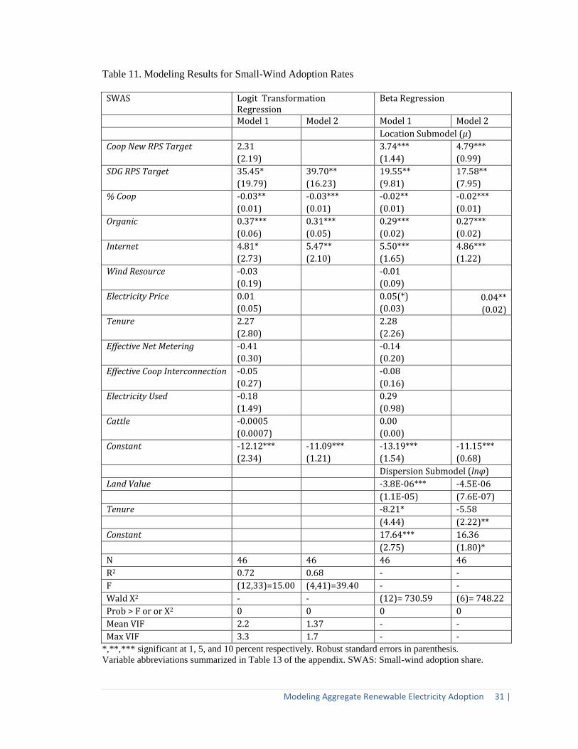
Modeling Aggregate Renewable Electricity Adoption 31 |
Table 11. Modeling Results for Small-Wind Adoption Rates
SWAS Logit Transformation Regression
Beta Regression
Model 1 Model 2 Model 1 Model 2
Location Submodel (μ)
Coop New RPS Target 2.31 3.74*** 4.79***
(2.19) (1.44) (0.99)
SDG RPS Target 35.45* 39.70** 19.55** 17.58**
(19.79) (16.23) (9.81) (7.95)
% Coop -0.03** -0.03*** -0.02** -0.02***
(0.01) (0.01) (0.01) (0.01)
Organic 0.37*** 0.31*** 0.29*** 0.27***
(0.06) (0.05) (0.02) (0.02)
Internet 4.81* 5.47** 5.50*** 4.86***
(2.73) (2.10) (1.65) (1.22)
Wind Resource -0.03 -0.01
(0.19) (0.09)
Electricity Price 0.01 0.05(*) 0.04** (0.05) (0.03) (0.02) Tenure 2.27 2.28
(2.80) (2.26)
Effective Net Metering -0.41 -0.14
(0.30) (0.20)
Effective Coop Interconnection -0.05 -0.08
(0.27) (0.16)
Electricity Used -0.18 0.29
(1.49) (0.98)
Cattle -0.0005 0.00
(0.0007) (0.00)
Constant -12.12*** -11.09*** -13.19*** -11.15***
(2.34) (1.21) (1.54) (0.68)
Dispersion Submodel (lnφ)
Land Value -3.8E-06*** -4.5E-06
(1.1E-05) (7.6E-07)
Tenure -8.21* -5.58
(4.44) (2.22)**
Constant 17.64*** 16.36
(2.75) (1.80)*
N 46 46 46 46
R2 0.72 0.68 - -
F (12,33)=15.00 (4,41)=39.40 - -
Wald Χ2 - - (12)= 730.59 (6)= 748.22
Prob > F or or Χ2 0 0 0 0
Mean VIF 2.2 1.37 - -
Max VIF 3.3 1.7 - -
*,**,*** significant at 1, 5, and 10 percent respectively. Robust standard errors in parenthesis.
Variable abbreviations summarized in Table 13 of the appendix. SWAS: Small-wind adoption share.

32 | Modeling Aggregate Renewable Electricity Adoption
Table 12. Normality Test for 2005 Logit Transformation Regression Models
PVAS SWAS
Statistic Test P value Test P value Skewness/Kurtosis test Χ2 1.41 0.493 4.30 0.12 Shapiro-Wilk W 0.98 0.62 0.96401 0.16 Shapiro-Francia W' 0.99 0.84 0.96346 0.14
PVAS: Solar-PV adoption share. SWAS: Small-wind adoption share
Summary and Concluding Remarks 33 |
Summary and Concluding Remarks
Adoption of solar and wind systems for generating on-farm electricity is not widespread,
but installations on the farm have increased greatly, especially since 2005 following a
trend of increased policy attention and investment in renewable energy. In 2009, policy
support intensified as the American Recovery and Reinvestment Act of 2009 (ARRA)
provided new incentives for the adoption of renewable energy systems, while an accruing
number of States continue to adopt incentives to promote renewable energy installations.
Though technology adoption is ultimately an individual farm-level choice determined by
specific farm-level characteristics, analyzing State-level variables can explain underlying
State variation in adoption rates, evaluate policy effectiveness, and even inform model
formulation of microlevel analysis. Our results suggest that some agricultural
characteristics are found to relate to higher adoption rates: States with more organic acres
per farm and more Internet connectivity have higher renewable electricity adoption rates.
Higher energy price and solar resource have a significant and positive relationship with
solar electricity adoption rates. For wind, economic influences do not appear to exhibit as
strong of a systematic relationship with State adoption rates, with the exception of
electricity price based on the beta regression. There are distinctions between wind and
solar energy, but the differences are not dramatic. For example, tenure is significantly
related to solar energy adoption but not wind adoption. Furthermore, wind energy
adoption is influenced by both new renewable RPS target and solar/DG RPS target, while
solar energy adoption is influenced by the solar/DG RPS target.
Electric cooperative prevalence in the State is found to have a negative relationship to
renewable electricity adoption share, which underlines the importance of policy
formulation. Out of the list of policy variables we considered, the RPS is actually the
only policy variable to show a large and systematic effect on State adoption rates. Our
results agree with Menz and Vachon (2006), Adelaja and Hailu (2008), and Yin and
Powers (2010), who found the RPS to be important for renewable electricity adoption;
however, their results applied to utility-scale renewable electricity adoption, while this is
the first study to show an impact at the distributed-generation scale. While both wind and
solar adoption rates have a significant relationship to the solar/DG RPS, only wind is also
significantly related to the new RPS standard. Our study does not find a systematic
relationship for other State policy instruments, at least in the form captured by our policy
variables. Financial policy instruments like rebates, grants, investment tax credits, and
production incentives do not appear to be correlated to State adoption rates for solar and
wind systems. Multivariate analysis further showed that effective (coop) net-metering
and interconnection fail to reveal a systematic relationship with renewable electricity
adoption rates on farms.
While Yin and Powers (2010) showed that net metering and interconnection were not
effective in increasing renewable generation, their analysis focused on utility capacity,
and we expected that effective net metering might have an impact on distributed

34 | Summary and Concluding Remarks
generation. Performance-based incentives, similarly to net metering, increase the positive
flow of revenues from the renewable electricity system and reduce its payback period.
Tax credits and direct payments, on the other hand, have the potential to reduce the high
upfront capital cost of renewable energy installations that are considered impediments to
adoption. For installation tax credits, the results further contradict the recent experience
with the Federal investment tax credit, which increased to 30 percent under the Energy
Policy Act of 2005 and resulted in a tripling of renewable energy installations between
2005 and 2008 (Sherwood 2010, 2009).
The incentives provided at the State level might indeed not influence adoption rates;
adoption decisions might instead be determined by farmer characteristics. It is also
possible that the effective incentives at the farm level are not sufficiently large to induce
a significant impact. Alternatively, incentive dummies and stringency averages might not
be adequately capturing the prices and incentives farms face. For example, the form of
the direct payments and benefits offered vary substantially from State to State, making a
comparable quantitative representation difficult. Furthermore, the dataset excludes any
incentives provided at the utility or local level, which could play a significant role in
adoption choices. Future examination at a more disaggregate level might provide more
insights.
The lack of systematic impact of those policies on solar and wind system adoption seems
to apply specifically to the agricultural sector, due to the smaller size bounds of
renewable electricity installations used by farmers until 2009 as well as to institutional
limitations. The negative relationship that the cooperative prevalence in electricity
distribution has with solar-PV and small-wind adoption suggests that the institutional
settings for rural energy policies are important determinants in the success of those
policies. It also suggests that USDA’s Rural Development Utilities Programs, which
helps rural utilities expand and keep their technology up to date while promoting rural
infrastructure development, is in a unique position to work with electric cooperatives to
promote distributed generation of renewable energy while increasing green job
opportunities (Rural Development a, b).
The study is the first to examine the role of electric cooperatives on solar and wind
system adoption on farms. It contributes to the literature of policy impacts on States’
renewable energy investment by providing insights on the effect of policies geared
towards distributed generation, specifically on renewable electricity production in
agriculture. Future work that could better categorize the different State policies might
provide better insights on the role of financial policy instruments in promoting small-
wind and solar installations in commercial, residential, as well as farm settings. The
results of this study can assist States as they further refine and focus their policies to
promote renewable electricity most effectively with limited budget resources. A more
detailed examination of farm-level data from OFREPS in combination with the policy,
institutional, and economic State-level variables identified in this report can provide a
fuller and more realistic interpretation of the determinants of adoption of solar and wind
energy generation.
References 35 |
References
Adelaja, S.J., and Y.G. Hailu. 2008. Effects of Renewable Portfolio Standards and Other State
Policies on Wind Industry Development in the US. Mimeo, Michigan State University.
Aitchison, J. 1986. The Statistical Analysis of Compositional Data. Chapman and Hall, New
York, NY.
Bazen, E. and M. Brown. 2009. Feasibility of Solar Technology (Photovoltaic) Adoption: A Case
Study on Tennessee's Poultry Industry. Renewable Energy 34(3).
Database of State Incentives for Renewables & Efficiency. Available at: www.dsireusa.org.
Accessed on April 11, 2011.
Database of State Incentives for Renewables & Efficiency Quantitative RPS Data Project. 2009.
December 2009 Archive. Available at: http://www.dsireusa.org/rpsdata/index.cfm.
Delmas, M. and M. Montes-Sancho. 2011. U.S. State Policies for Renewable Energy: Context
and Effectiveness. Energy Policy. 39(5)
Denholm, P. Margolis, R.M., Ong, S. and B. Roberts. 2009. Breakeven Cost for Residential
Photovoltaics in the United States: Key Drivers and Sensitivities. NREL TP-6A2-46909.
National Renewable Energy Laboratory (NREL), Department of Energy (DOE).
http://www.nrel.gov/docs/fy10osti/46909.pdf (Accessed September 10, 2010)
Dillman, D.A., Roosa, E.A. and J.J. Dillman. 1983. Lifestyle and Home Energy Conservation in
the United States: The Poor Accept Life-style Cutbacks While the Wealthy Invest in
Conservation. Journal of Economic Psychology 3 (Sep).
Durham, C., Colby, B. and M. Longstreth. 1988. The Impact of State Tax Credits and Energy
Prices on Adoption of Solar Energy Systems. Land Economics 64 (4).
Edwards, J.L., Wiser, R.H., Bolinger, M., and T. Forsyth. 2004. Building a Market for Small
Wind: The Break-Even Turnkey Cost of Residential Wind Systems in the United States.
Ernest Orlando LBNL-54865. Lawrence Berkeley National Laboratory (LBNL).
http://emp.lbl.gov/sites/all/files/REPORT%20lbnl%20-%2054865.pdf (Access march 15,
2013)
Evans, J.R. and D.L. Olson. 2003. Statistics, Data Analysis, and Decision Modeling. Prentice-
Hall, Upper Saddle River, NJ.
Food and Agriculture Organization. 2000. Solar Photovoltaics for Sustainable Agriculture and
Rural Development. Environment and Natural Resources Working Paper No. 2. Rome,
Italy: Food and Agriculture Organization. Available at:
http://www.fao.org/sd/EGdirect/EGre0057.htm (Accessed September 14, 2012).
Freeing the Grid. Available at: http://www.gracelinks.org/1179/freeing-the-grid. Accessed on
January 11, 2013.
36 | References
Fujii, E.T., and J. Mak. 1984. A Model of Household Electricity Conservation Behavior, Land
Economics 60.
KAEC. http://www.kaec.org/faq.htm. Accessed on July 1, 2012.
Katzman, M.T., and R.W. Matlin. 1978. Economics of Adopting Solar Energy Systems for Crop
Irrigation. American Journal of Agricultural Economics 60.
Kieschnick, R., and McCullough B.D. 2003. Regression Analysis of Variates Observed on (0, 1):
Percentages, Proportions, and Fractions. Statistical Modeling 3
Knowler, D. and B. Bradshaw. 2007. Farmers’ Adoption of Conservation Agriculture: A Review
and Sybthesis of Recent Research. Food Policy 32.
Labay, D. and T. Kinnear. 1981. Exploring the Consumer Decision Process in the Adoption of
Solar Energy Systems. Journal of Consumer Research 8 (Dec).
Long, J. 1993. An Econometric Analysis of Residential Expenditures on Energy Conservation
and Renewable Energy Sources. Energy Economics 15.
Menz, F.C., and S. Vachon. 2006. The effectiveness of different policy regimes for promoting
wind power: Experiences from the States. Energy Policy 34.
Mills, B.F. and J. Schleich. 2009. Profits or Preferences? Assessing the Adoption of
Residential Solar Thermal Technologies. Energy Policy 37.
National Agricultural Statistics Service. 2011. On-Farm Renewable Energy Production Survey
2009. Washington, DC: U.S. Department of Agriculture.
National Agricultural Statistics Service. 2009a. Census of Agriculture 2007. Washington, DC:
U.S. Department of Agriculture.
National Agricultural Statistics Service. 2009b. Farm and Ranch Land Irrigation Survey 2008.
Washington, DC: U.S. Department of Agriculture.
National Agricultural Statistics Service. 2004. Farm and Ranch Land Irrigation Survey 2003.
Washington, DC: U.S. Department of Agriculture.
National Renewable Energy Laboratory. 2009. Lower 48 PV Low Resolution. U.S. Department of
Energy. Available at: http://www.nrel.gov/gis/data_solar.html. Accessed on April 11,
2012.
National Renewable Energy Laboratory. 2003. Lower 48 Wind Low Resolution. U.S. Department
of Energy. Available at: http://www.nrel.gov/gis/data_wind.html. Accessed on April 11,
2012.
O’Doherty, J., Lyons, S. and R. Tol. 2008. Energy-using Appliances and Energy-saving Features:
Determinants of Ownership in Ireland. Applied Energy 85 (7).
Ostlund, L.E. "Perceived Innovation Attributes as Predictors of Innovativeness." Journal of
Consumer Research 1(1974): 23-29.
References 37 |
Robinson, W.S. 1950. Ecological Correlations and the Behavior of Individuals. American
Sociological Review 15( 3: Jun)
Rose, J. 2008. Freeing the Grid 2008: The Best and Worst Practices in State Net Metering
Policies and Interconnection Procedures. Network for New Energy Choices.
Rural Development. U.S. Department of Agriculture. Available at:
a. http://www.rurdev.usda.gov/utilities_LP.html , and
b. http://www.rurdev.usda.gov/UEP_HomePage.html. Accessed on April 11, 2013.
U.S. Energy Information Administration. 2013. Monthly Energy Review. February 2013.
Avaialable at: http://www.eia.gov/totalenergy/data/monthly/pdf/mer.pdf. Accessed on
March 10, 2013.
U.S. Energy Information Administration. 2012. Electric Power Monthly. March 2012. Available
at: http://www.eia.gov/electricity/monthly/current_year/march2012.pdf. Accessed on July
10, 2012.
U.S. Energy Information Administration. 2012a. Electric Sales, Revenue, and Average Price.
Form EIA-861. Annual Electric Power Industry Report 2008. Available at:
http://www.eia.gov/electricity/sales_revenue_price/. Accessed on July 10, 2012.
U.S. Energy Information Administration. 2012b. Gasoline and Diesel Fuel Update. Full History
Dataset. Washington DC: U.S. Department of Energy.
U.S. Energy Information Administration. 2012c. Form EIA-861 data files. Annual Electric Power
Industry Report 2008. Available at:
http://www.eia.gov/electricity/data/eia861/index.html. Accessed on July 10, 2012.
U.S. Energy Information Administration. 2011. Annual Energy Review 2009. Washington, DC.
Available at: http://www.eia.gov/electricity/annual/. Accessed on July 10, 2012.
U.S. Energy Information Administration. 2010. Annual Energy Review 2008. Washington, DC.
Available at: http://www.eia.gov/electricity/annual/. Accessed on July 10, 2012.
U.S. Energy Information Administration. 2009b. Annual Energy Review 2007. Washington, DC.
Available at: http://www.eia.gov/electricity/annual/. Accessed on July 10, 2012.
U.S. Energy Information Administration. 2009a. Petroleum Marketing Annual 2008. Explanatory
Notes. Washington DC: U.S. Department of Energy.
Sardianou, E. 2007. Estimating Energy Conservation Patterns of Greek Households. Energy
Policy 35.
Sawyer, S.W., A. Sorrentino, and R. M. Wirtshafter. 1984. Solar Energy Adoption Patterns in the
United States. Energy Systems and Policy 8( 2)
Sherwood, L. 2010. U.S. Solar Market Trends 2009. InterState Renewable Energy Council.
Sherwood, L. 2009. U.S. Solar Market Trends 2008. InterState Renewable Energy Council.
38 | References
Shrimali, G., and J. Kniefel. "Are government policies effective in promoting deployment of
renewable electricity resources?" Energy Policy 39(2011): 4726–4741.
Skinner, J., and D. Staiger. 2007. Technology Adoption from Hybrid Corn to Beta-Blockers, ed.
C.M. Hulten, University of Chicago Press and National Bureau of Economic Research
(NBER).
Smithson, M. and J. Verkuilen. 2006. A Better Lemon Squeezer? Maximum Likelihood
Regression with Beta-Distributed Dependent Variables. Psychological Methods 11(1)
Walsh, M. 1989. Energy Tax Credits and Housing Improvement. Energy Economics 11.
Willis, K., Scarpa, R., Gilroy, R., and N. Hamza. 2011. Renewable Energy Adoption in
an Ageing Population: Heterogeneity in Preferences for Micro-generation
Technology Adoption. Energy Policy 39.
Xiarchos, I., and B. Vick. 2011. Solar Energy Use in U.S. Agriculture: Overview and Policy
Issues. Washington, DC: U.S. Department of Agriculture, Office of the Chief Economist,
Office of Energy Policy and New Uses.
Yin, H., and N. Powers. Do State Renewable Portfolio Standards Promote In-State Renewable
Generation? Energy Policy 38(2010): 1140–1149.

Appendix 39 |
Appendix Table 13. Variable Abbreviations
Diesel Price Diesel Price per Gallon
Electricity Price Average Residential Retail Electric Price per Kilowatt Hour
PV Resource Solar potential, (4.2-6.2)
Wind Resource Wind classification, (1-5)
% Coop Percentage of Customers Served by Electric Cooperatives
NR RPS Target Renewable Portfolio Standard Target for New Renewables
Coop Exemption Cooperative exemption from Renewable Portfolio Standard
Coop NR RPS Target Cooperative Specific Renewable Portfolio Standard Target for New Renewables
SDG RPS Target Renewable Portfolio Standard Target for Solar/Distributed Generation
Coop SDG RPS Target Cooperative Specific Renewable Portfolio Standard Target for Solar/Distributed Generation
Net Metering Net Metering Policy, (0,1)
Effective Net Metering Effective Net Metering Policy, (0,1)
NM P. Excess Electricity Net Metering Price for Excess Electricity per Kilowatt Hour
Cooperative Net Metering Net Metering Policy for Cooperatives, (0,1)
Effective Coop Net Metering
Effective Net Metering Policy for Cooperatives, (0,1)
Interconnection Interconnection Policy, (0,1)
Effective Interconnection Effective Interconnection Policy, (0,1)
Coop Interconnection Interconnection Policy for Cooperatives, (0,1)
Effective Coop Interconnection
Effective Interconnection Policy for Cooperatives, (0,1)
Incentive Financial Incentive, (0,1)
ITC Investment Tax Credit, (0,1)
PI Production Incentive, (0,1)
DP Grant and Rebate Program, (0,1)
ITC rate, % Investment Tax Credit Rate, Percent
PI rate, $/kWh Production Incentive Rate per Kilowatt Hour
ITC Years Investment Tax Credit, Years since Enactment
PI Years Production incentive, Years since Enactment
DP Years Grant and Rebate Program, Years since Enactment
REAP # Number of Projects funded by Rural Energy for America Program
REAP $ Dollars distributed to projects funded by Rural Energy for America Program
Fuel Expense Fuel Expense by Operation
Electricity Expense Electricity Expense by Operation
Electricity Used Electricity Used by Operation
Funding Share Funding Share Supporting the Cost of Photovoltaic and Small-Wind Installations
Net Cash Income Net Cash Income by Operation
Land Value Land Value by Operation
Machinery Value Machinery Value by Operation
Organic Organic Acres by Operation
Conservation Conservation Acres by Operation
Fruit Share of Fruit Operations in State
Cattle Share of Cattle Operations in State
Tenure Share of Operations Tenure with Full Tenure of Operated Land
Internet Share of Operations Connected to the Internet
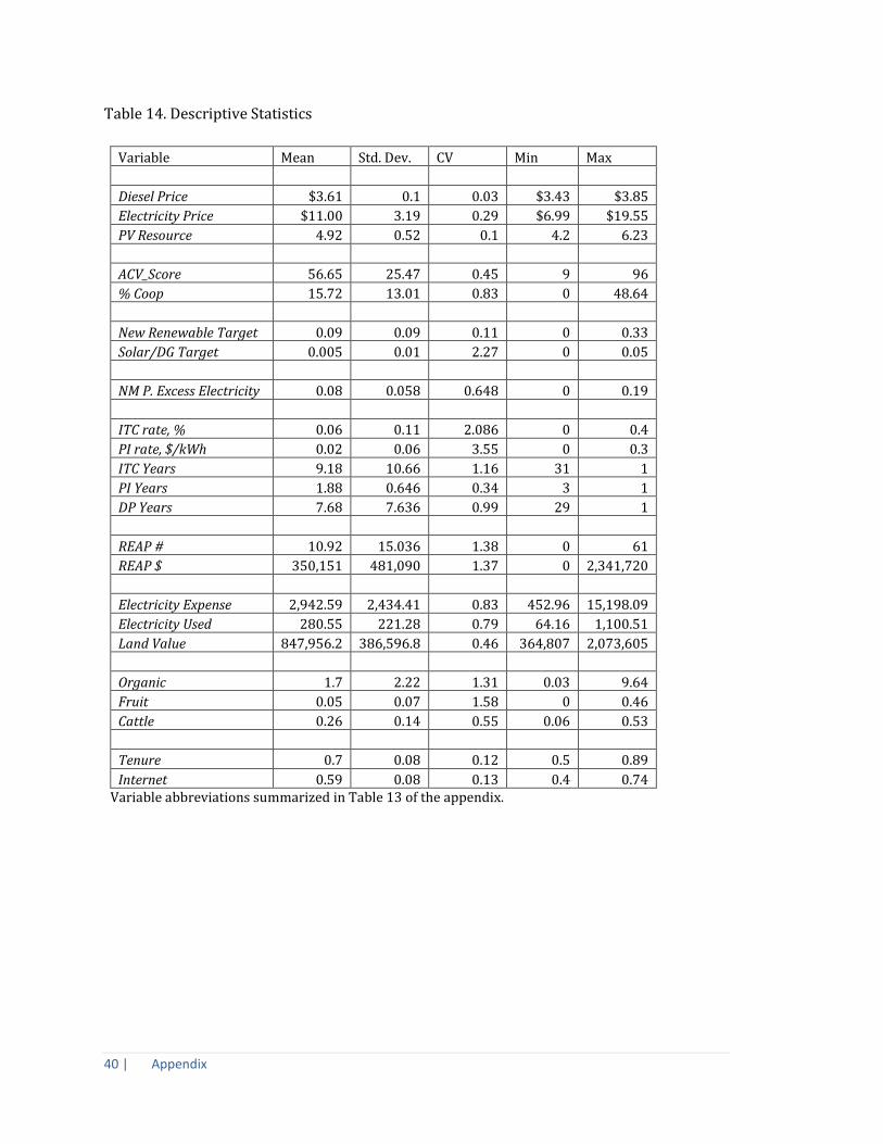
40 | Appendix
Table 14. Descriptive Statistics
Variable Mean Std. Dev. CV Min Max
Diesel Price $3.61 0.1 0.03 $3.43 $3.85
Electricity Price $11.00 3.19 0.29 $6.99 $19.55
PV Resource 4.92 0.52 0.1 4.2 6.23
ACV_Score 56.65 25.47 0.45 9 96
% Coop 15.72 13.01 0.83 0 48.64
New Renewable Target 0.09 0.09 0.11 0 0.33
Solar/DG Target 0.005 0.01 2.27 0 0.05
NM P. Excess Electricity 0.08 0.058 0.648 0 0.19
ITC rate, % 0.06 0.11 2.086 0 0.4
PI rate, $/kWh 0.02 0.06 3.55 0 0.3
ITC Years 9.18 10.66 1.16 31 1
PI Years 1.88 0.646 0.34 3 1
DP Years 7.68 7.636 0.99 29 1
REAP # 10.92 15.036 1.38 0 61
REAP $ 350,151 481,090 1.37 0 2,341,720
Electricity Expense 2,942.59 2,434.41 0.83 452.96 15,198.09
Electricity Used 280.55 221.28 0.79 64.16 1,100.51
Land Value 847,956.2 386,596.8 0.46 364,807 2,073,605
Organic 1.7 2.22 1.31 0.03 9.64
Fruit 0.05 0.07 1.58 0 0.46
Cattle 0.26 0.14 0.55 0.06 0.53
Tenure 0.7 0.08 0.12 0.5 0.89
Internet 0.59 0.08 0.13 0.4 0.74 Variable abbreviations summarized in Table 13 of the appendix.