export incentives, financial constraints, and the (mis...
TRANSCRIPT

Export Incentives, Financial Constraints, and the (Mis)Allocation of Credit:
Micro-Level Evidence from Subsidized Export Loans
Bilal H. Zia*
(World Bank Finance Research Group)**
First Draft: October 2005 (MIT Economics Job Market Paper)
This Draft: December 2006 (Forthcoming, Journal of Financial Economics)
Abstract The provision of subsidized credit to exporting firms is widespread in emerging markets. To what extent are such incentives useful in alleviating financial constraints and promoting firm growth? In terms of efficiency, are more financially constrained firms allocated a greater share of credit? This paper combines an exogenous shock to the supply of subsidized credit with unique loan-level data from the export sector in Pakistan to identify the impact and allocation of such financial incentives. The removal of subsidized credit causes a significant decline in the exports of privately owned firms, while the exports of large, publicly listed, and group network firms are unaffected. Publicly listed firms make no significant adjustments to their balance sheets, and only their profits are reduced, indicating that they are financially unconstrained. Nearly half of all subsidized loans are assigned to such firms, implying a substantial misallocation of credit. Real economic costs of this misallocation in terms of output loss to privately owned firms are estimated to be at least 0.75% of GDP. The analysis also shows that productivity differences cannot explain the heterogeneous effects across firms.
JEL Classifications: F13, G15, G18, G21
* World Bank Finance Research Group, 1818 H Street NW, Washington DC 20433. [email protected]; Tel: 202-458-1433; Fax: 202-522-1155. ** I thank my advisors at MIT, Abhijit Banerjee, Esther Duflo, and Antoinette Schoar for guidance, the State Bank of Pakistan for allowing access to their data and for substantial logistical support. I also thank David Autor, Shawn Cole, Mihir Desai, Todd Gormley, Asim Khwaja, Atif Mian, and an anonymous referee for detailed comments on earlier drafts. Finally, I am grateful to seminar participants at Amsterdam Business School, Federal Reserve Board, Harvard Business School, MIT, Oregon Lundquist Business School, Stockholm School of Economics, and the World Bank for comments and useful discussions. The analysis and conclusions in this paper are my own, as are all errors and omissions.

The provision of subsidized credit to domestic firms is an important policy goal in many emerging
markets, and is particularly widespread in export sectors.1 Several East Asian “miracle” economies –
Japan, Korea, and Taiwan in particular – relied heavily on export credit policies, while enjoying export
growth rates in excess of 20 percent during the latter half of the 20th century (Kokko, 2002). The recent
push towards globalization and WTO led market-oriented reform, however, has called into question the
success of government assisted export promotion, and has prescribed a strict rollback of such policies
worldwide. In light of these developments, it is important to understand the impact of removal of such
financial incentives on the real outcomes of beneficiary firms, especially small privately owned firms that
may otherwise be financially constrained.
This paper addresses two important and related research questions: (a) to what extent is subsidized
credit useful in alleviating financial constraints and promoting firm-level export growth? And (b) how
efficiently is such credit allocated across targeted firms? These questions are interesting not only because
credit subsidies are so common, but also because they can provide insight into the broader issues of
financial development and growth in emerging markets. From a theoretical perspective, Banerjee and
Newman (2004) argue that financial subsidies help correct allocative distortions created by poor credit
markets, and therefore can boost export growth. A direct implication of their model is that for credit
subsidy programs to be efficient, the subsidies should be allocated to financially constrained firms. Yet,
there are several reasons why this may not be the case. Rajan and Zingales (2003), for instance,
emphasize the role of private interest groups in retarding financial development, which in the context of
subsidies would mean capture by firms that have greater influence – typically the large unconstrained
ones. Similarly, Johnson and Mitton (2003) find evidence that firms with strong political connections
benefit from a higher level of subsidies. More generally, papers such as Khwaja and Mian (2005), Dinc
(2005), and Cole (2004) carefully examine how political connections lead to cheaper lending. The
1 Government support for export sectors is well documented in the trade literature (see for instance, Bernard and Jensen, 2001; Das, Roberts, and Tybout, 2004). Export sectors are a major source of foreign currency reserves, contribute significantly to GDP growth, and employ a large share of the domestic workforce.
2

contribution of my paper is that I am able to distinguish which types of firms are financially constrained,
and identify the size and mechanism of the “capture” or misallocation of credit to firms that are otherwise
financially unconstrained.
There are several empirical challenges involved in this analysis. The lack of micro-level data from
emerging markets is a major problem, especially on small privately owned firms for whom these issues
are most relevant. In addition, it is difficult to cleanly identify which types of firms are financially
constrained. The corporate finance literature has traditionally employed the sensitivity of firm investment
to current cash flow, with high sensitivity firms being regarded as financially constrained.2 However, this
approach has been criticized for potential endogeneity issues.3 Recent work has tried alternative routes
such as using oil price changes to look at the outside-industry investment of oil companies (Lamont,
1997), studying systematic relationships between cash savings and cash flow within firms (Almeida, et.
al., 2004), and exploiting non-linear funding rules in pension plans to identify the dependence of
investment on internal financial resources (Rauh, 2006).
My paper identifies financial constraints through an exogenous shock to the supply of subsidized
credit. I take advantage of a unique loan-level panel dataset from the export sector of an emerging market,
Pakistan. The Central Bank of Pakistan provides subsidized loans through the commercial banking sector
to domestic firms that export an eligible set of commodities. The dataset contains detailed loan and export
output information for the entire universe of firms utilizing these subsidies. I exploit an exogenous change
in eligibility that resulted in the subsidies being discontinued for a specific commodity, cotton yarn, and
compare outcomes before and after the policy change for yarn and non-yarn textile firms. Importantly, I
show that the removal of subsidies for yarn firms was uncorrelated with the export performance of these
firms.
2 See Fazzari, Hubbard, and Petersen (1988) for an introduction to this literature; Hubbard (1998) for a detailed survey; Poterba (1988) and Kaplan and Zingales (1997, 2000) for a critique. 3 See for instance, Poterba (1988) and Alti (2003).
3

I find that following the policy change, yarn firms are unable to replace their subsidized credit with
market-rate loans, and their exports fall sharply. However, these results are heterogeneous across different
types of firms. In particular, the total loans and exports of large, publicly listed firms are unaffected by the
removal of credit subsidies, while those of privately owned firms are significantly affected. My analysis
suggests that these differences arise because privately owned firms are financially constrained, while
large, publicly listed firms are unconstrained. Further, within the subset of privately owned firms, I find
that firms that are part of corporate group networks, are larger, or have relationships with multiple banks
are able to overcome their constraints better.
Next, I provide evidence that credit subsidies to publicly listed firms are substantially misallocation.
Using balance sheet data, I show that the additional cost of financing after the removal of credit subsidies
is fully absorbed in the “interest expenses” entry in the profit and loss accounts of these firms. Moreover,
there is no significant change in assets, capital structure, long-term investments, or total sales, rather only
an adjustment in profits. In fact, the magnitude of the decline in profits matches almost one-to-one with
the increase in borrowing costs. These findings suggest that the subsidies simply provided the publicly
listed firms with an opportunity to earn windfall profits. Hence, not only are publicly listed yarn firms
financially unconstrained, but the incentives from export subsidies are infra-marginal for these firms –
that is, they would have borrowed the same amount irrespective of the credit subsidies.
In terms of economic costs, I show that nearly half of the subsidized credit prior to the policy change
is assigned to publicly listed firms, precisely the firms that do not need it. At the same time, I show that a
large majority of privately owned firms are financially constrained in that their exports are highly
sensitive to the removal of subsidized credit. Among privately owned firms, even the more productive
ones are financially constrained, which indicates that the opportunity cost of the misallocated funds is
significant. Using direct export output measures, I estimate the output loss due to this misallocation to be
at least 0.75% of GDP. These results provide compelling evidence of the inefficient “capture” of credit
subsidies by the publicly listed firms.
4

I argue that the exports of privately owned firms decline sharply because they are more financially
constrained than others. An alternative interpretation of these results is that privately owned firms are
simply less productive than other firms, and that exporting is not feasible without subsidized credit.
Removing subsidies for these firms would then be the efficient thing to do. Indeed, Bhagwati (1996) and
others have argued that export subsidies are economically wasteful because they aid in the preservation of
low-quality firms. Recent trade literature, following Melitz (2003), also argues that productivity
differences across firms influence the extensive margin of trade. My paper, however, provides evidence
against this alternative interpretation. First, concentrating on exporting firms is an advantage since these
are typically the better performing firms in the economy.4 Second, prior to the change in subsidy policy,
more than 95% of firms in the dataset (private, listed, and group) supplement their subsidized credit with
some borrowing at regular market rates from banks. This finding suggests that it would be feasible for
firms to continue exporting even without the credit subsidy since their marginal product curves lie above
the market lending rate. Third, I directly test whether productivity differences matter and do not find
evidence that less productive firms are affected more by the removal of subsidies.
In terms of public policy, while I find that export subsidies help alleviate financial constraints, I also
show that a substantial portion of these subsidies are allocated to financially unconstrained firms. The
analysis highlights the risks involved in having a subsidized credit scheme that does not have strict
qualification rules based on observable firm characteristics, and provides insight into what these
characteristics might be. Further, in the spirit of Rajan and Zingales (2003), this paper quantifies the size
and mechanism of the misallocation of credit, and hence identifies a channel of financial and private-
sector underdevelopment in emerging markets.
This paper is organized as follows. The next section describes the export subsidy scheme in Pakistan,
its institutional environment, and the policy change. Section II explains the data, and Section III outlines
the conceptual framework, identification strategy, and empirical specifications. Sections IV and V present
4 See Section VI for evidence and a detailed discussion.
5

results of the empirical analysis. Section VI performs a series of robustness checks, and Section VII
concludes.
I. Institutional Setting and Policy Change Details
A. The Textile Export Sector in Pakistan
The textile industry in Pakistan presents a particularly relevant setting in which to study the effects of
export credit subsidies. The exporting sector of the country is dominated by the textile industry, which
accounts for 67% of Pakistan’s total exports (SBP Annual Report, 2003). These exporters are price-takers
on the international market,5 which allows the quantity effects of subsidy provision to be identified
independent of changes in price. In addition, firms within the textile industry are heavily export-oriented
with more than 70% of industry production sold overseas.
A large proportion of these textile exports are supported by government loan subsidies provided
under the Export Finance Scheme (EFS). EFS accounts for 38% of country-wide exports and 42% of total
exports in the textile sector. Hence, the textile sector accounts for the majority of Pakistan’s exports and is
also the main beneficiary of the government-sponsored subsidy scheme.
B. The Credit Subsidy Scheme in Detail
The Government of Pakistan sponsors and operates the Export Finance Scheme (EFS) through the State
Bank of Pakistan (SBP), which is the central bank of the country. The scheme has been operational since
1973 and provides working capital loans to exporters of eligible commodities at subsidized interest rates.
The scheme works entirely through the formal banking sector, and banks earn a fixed 1.5% spread on the
loans that they provide under EFS. All banks in Pakistan face the same regulatory environment, which
allows the SBP to operate EFS through the entire commercial banking sector of the country.6
5 Pakistani Textiles have a 2% share in the global market.
6

Credit provided under EFS comprises short-term working capital loans with a maturity of 180 days.
Commercial banks extend credit to firms and then receive refinancing from the SBP, which also monitors
and regulates the entire scheme. An original export order is required before a loan can be approved, and
copies of this document are forwarded to the regional SBP field offices at loan signing. At the time of
loan repayment, firms are required to submit their sales invoice along with shipping documents and a
customs appraisal letter. Details provided in these documents are matched with the original export order,
and copies are then forwarded to the SBP.7 Fines are imposed by the SBP if firms fail to provide shipping
documents, even if they are able to repay their loan amounts. Firms with overdue fines are barred from
further EFS borrowing until their fine balances are cleared. The imposition of fines, however, is quite rare
– as summary statistics in Table II (b) show, a fine for late submission is imposed on less than 3% of all
EFS loans, whereas complete non-submission occurs in less than 0.5% of loans.
There is a limit on how much EFS credit any single firm can receive in a year, dependent on its
market valuation. Specifically, private firms are allowed to borrow up to 5 times their capital and
reserves, and publicly listed firms 2 times their capital and reserves. The motivation for these different
limits is that publicly listed firms have access to other forms of financing such as share-holder equity that
are not available to private firms. In addition, each bank is assigned a sanctioned limit by the SBP based
on the size of its equity and reserves, which indicates the maximum amount of EFS credit it can extend.
The size of the EFS subsidy on average is 6 percentage points (i.e., market rate - EFS rate = 6%),
though in recent years it has been much lower. This subsidized rate of interest, by EFS rules, is consistent
across all banks and firms. Figure I plots the time-series trend in EFS rate against the market lending rate
and the 6-monthly Treasury-bill (T-bill) rate. Until very recently, the EFS lending rate was set on an ad-
hoc basis, with some relation to the T-bill rate. Starting in June 2002, however, under pressure from the
6 As of June 2003, there were 6 government-owned, 24 foreign, and 12 private domestic commercial banks in Pakistan, all of which participated in EFS. While there have been efforts to introduce Islamic shariah law in the banking sector, it has not had any substantial functional impact on bank operations. For all practical purposes, banking in Pakistan is in line with international standards, with deposit and lending rates determined by the market. 7 If the shipping date provided in the original export order is beyond the 180 day loan term, then firms are required to submit the shipping documents within 30 days of that date.
7

International Monetary Fund (IMF) to implement more market-oriented policies, the EFS rate was strictly
pegged a few basis points above the T-bill rate.
C. Policy Change Details
Access to EFS loans is not open to all firms. Specifically, SBP maintains a negative list of products not
eligible for subsidized loans. The range of items on this list is quite diverse, from petroleum products and
crude minerals to animal hides and fur skins. Interviews with SBP officials indicate that the motivation
for the negative list is to encourage the export of value-added goods rather than basic raw materials.
A major change in the EFS eligibility criteria was announced by SBP in late 2000 and came into
effect in June, 2001. Specifically, in an attempt to focus more on value-added goods, the SBP decided to
exclude the export of cotton yarn from EFS and added it to the negative list. At the time of the policy
change, yarn spinners occupied a very large fraction of the EFS-supported textile industry – pre-period
loans to yarn spinners comprised on average 30% of all EFS loans to the textile sector. The policy change
was announced, retracted, and a revised version issued through a series of SBP circulars from June to
December, 2000. The initial version called for an immediate cessation of loans for yarn while the revised
version, issued very soon afterwards, allowed the EFS facility to continue until the end of the fiscal year.
The data clearly shows that EFS loans for yarn exports cease abruptly in June, 2001.
My empirical analysis relies on the assumption that the policy change was uncorrelated with prior
export performance of yarn firms. It is, therefore, important to understand whether the policy change was
exogenous. I show later in the paper that this was the case. That is, the growth of yarn exports prior to the
policy change was very similar to that of non-yarn exports.
II. Data and Summary Statistics
This paper brings together three original datasets, two of which were collected specifically for this
research. The first has detailed loan-level credit and output information for all exporting firms operating
under the umbrella of EFS from June, 1998 to June, 2003. The second dataset provides similar detailed
8

loan-level information for total corporate loans given out by banks in all of Pakistan for the same sample
period. Finally, the third dataset consists of detailed annual accounts for all publicly listed firms in
Pakistan for the sample period of interest.
A. Exports Database
The loan-level export database used in this paper provides detailed loan and export output information for
all firms (publicly listed and private) borrowing under EFS. Each row in the database corresponds to a
firm-loan entry. For each of these entries, the dataset provides information on exporter name and location,
importer name and location, exporter industry and commodity type, loan amount, export amount, and
default amount, if any. Overall, the dataset is a panel from 1998 to 2003, comprising 97,937 unique loans
given to 3,122 unique firms over the 5-year period. The textile sector received 50,661 of these loans, and
the sector comprised 1,120 firms. This data constitutes the entire universe of EFS loans and
corresponding exports for the given period.
As discussed earlier, yarn exporters have been excluded from EFS since June, 2001. Since the export
data is only for firms operating within the scheme, these firms disappear from the dataset after this date.
However, data on total exports for yarn and non-yarn textile firms was collected from commercial banks
for the period June, 2000 to June, 2003. Due to less stringent reporting requirements prior to 2000, this
data was not available for earlier years.
Tables I (a) and I (b) present summary statistics for several loan-level variables from the EFS data.
These include pre-period averaged loan amounts, export valuations, and net fines imposed for late
submission of shipping documents. The figures are reported for all firms and also separately for yarn and
other textiles. Table I (b) shows that the average loan amounts for yarn are on average much larger than
those for other textiles, and correspondingly, average exports per loan are also greater for yarn.
9

B. Total Loans Database
The total loans database, like the EFS data, is provided by the SBP and is unique both in terms of its
coverage and detail. It contains yearly information on the entire universe of total corporate bank loans
outstanding in Pakistan for the 5-year panel from 1998 to 2003. The data is at the level of bank,
borrowing firm, and year, and traces the history of lending with information on the amount of loan and
interest outstanding, type of loan (working capital, fixed investment, or other), and any defaults on these
loans. In addition, this data provides names and national tax IDs for the board of directors of all firms.
Since the empirical strategy used in this paper does not exploit differences across banks but rather
differences across firms, the total borrowing and other variables of interest are aggregated to the level of
the firm. Firm-level variables provided in this dataset are matched with EFS firms to create a unified
panel spanning 5 years.8 Panel A of Table I (c) shows brief summary statistics on total loans and default
rates, restricted to the subset of EFS matched firms. Approximately 50% of firms in the dataset have
positive fixed investment loans from banks, but these do not adjust significantly around the EFS policy
change. This is understandable since EFS loans are working capital loans and tied in closely with the
overall working capital portfolio of firms. Hence, the analysis in this paper will focus on working capital
loans. Another aspect to note from the table is that the default rate on loans to exporters is fairly low, with
the 75th percentile corresponding to a firm with zero default.
C. Corporate Sector Financial Accounts
While the EFS and total lending databases provide detailed loan and output information, they do not
contain any firm-level attributes such as size of assets, equity, total sales, or trade credit. This paper
supplements these two datasets with corporate annual accounts data obtained directly from the Securities
and Exchange Commission of Pakistan (SECP). This database consists of audited financial accounts for
8 A name-matching algorithm was used to match firms across the two datasets. This was followed by a series of manual cross checks to ensure that the match was correct. More than 90% of EFS firms were successfully matched.
10

all publicly listed companies for a panel of over 10 years, starting in 1990. These firms are required by
law to file their annual reports with the SECP.
Firms in this dataset are matched with their EFS and total loan information to create a firm-level
dataset with exports, total loans, assets, and liabilities for all publicly listed firms borrowing under EFS.
Panel B of Table I (c) presents summary statistics for some borrowing firm attributes from the corporate
financial accounts data.
III. Conceptual Framework and Identification
A. Conceptual Framework
Access to capital is key to identifying the firm-level response to the removal of subsidized credit. In order
to establish predictions on the effects of financial access constraints on firms, it is important to first
highlight that the Bank Lending Channel in Pakistan is also constrained – that is, credit supply is quite
inelastic. Khwaja and Mian (2006a) exploit an exogenous shift in source funding to show that bank credit
supply in Pakistan is fairly rigid. These findings are very relevant for this paper because once subsidies
are removed, in order to continue lending to firms that were previously being financed through the
Central Bank provided EFS funds, commercial banks would now have to finance them through their own
deposit base. With an inelastic credit supply, however, commercial banks would not be able to
compensate for the removal of subsidies by lending more from their own reserves.
Although this mechanism predicts a lack of loan substitution for all firms, it cannot explain
heterogeneity across firms, in that some firms are able to make this substitution, while others are not. An
important mechanism that can lead to such heterogeneous effects is the simultaneous large upward shift in
interest rates – firms substituting EFS borrowing with regular bank lending would have to pay a
significantly higher interest rate. Several theoretical models in the banking literature, starting from Stiglitz
and Weiss (1981), demonstrate that credit may be rationed in equilibrium if information asymmetries
exist between borrowers and lenders, and that the level of the interest rates charged has direct
implications for the riskiness of loans. Specifically, a higher interest rate may induce only firms with
11

riskier project to demand loans (adverse selection), and similarly may induce mangers to undertake riskier
projects (moral hazard). In order to formalize this concept and generate testable empirical predictions, it is
useful to think in terms of the following very simple, stylized model:9
Firms face a gross production process F(.) and want to make an investment I in a particular project.
Each firm can invest its own resources W in the project, and therefore needs to borrow (I-W). The gross
interest rate for this loan amount is r, and the repayment amount is thus r(I-W). Without loss of generality,
assume that the opportunity cost of investment is zero.
Lets now introduce a moral hazard problem. Since exporting firms produce on the basis of an export
order, the type of moral hazard introduced here is not based on managerial choice that affects the
probability of success of the project, as in Holmstrom and Tirole (1997), but rather is based on the
possibility that firms may renege on the repayment of their bank loans ex post of project completion.
Specifically, assume that firms can expend some resources proportional to their investment, Iα , and
renege on the repayment of their loans. Iα can be thought of as the actual costs associated with reneging
on loan terms, penalties towards future borrowing, or reputation costs associated with default. What is
important for the analysis is that α varies across different types of firms. This assertion can be justified
by way of illustration: firms that are publicly listed on the stock market, for instance, face greater scrutiny
and market discipline, and also face greater reputation costs of default than smaller, less established,
privately-owned firms. Publicly listed firms are also required, by law, to submit balance sheets to the
stock exchange using SECP approved auditors, thus making it more costly to misreport statements. In this
illustration, α will be higher for publicly listed firms than for privately-owned firms.10
Given this setup, firms face the following Incentive Compatibility (IC) constraint:
IIFWIrIF α−≥−− )()()( (1)
9 This formalization draws on previous work by Banerjee (2001) and Holmstrom and Tirole (1997). 10 Similar predictions can be derived comparing firms belonging to corporate groups vs. non-group affiliated firms. This comparison and other similar ones are discussed in detail later in Section IV of the paper.
12

Rewriting (1):
)( α−
≤rrWI (2)
In equilibrium, the amount a firm can borrow will be:
⎟⎟⎟
⎠
⎞
⎜⎜⎜
⎝
⎛
−=⎟
⎠⎞
⎜⎝⎛
−=−=
11)(α
αα
rW
rWWIB (3)
This simple formalization provides the following useful comparative statics:
0>∂∂αB
CS(a)
0<∂∂
rB
CS(b)
02
<∂∂
∂αrB
CS(c)
CS(a) simply states that the amount banks will be willing to lend is an increasing function of α - the
more costly it is for firms to renege on repayment of loans, the more banks will be willing to lend. CS(b)
and CS(c) provide the main predictions of the model. CS(b) states that an increase in interest rates will
result in a decrease in lending by banks because of the moral hazard issue, however, according to CS(c),
this effect will be diminished for firms with higher α ’s. Moreover, these two derivatives combined
predict that lending will decrease more for firms for whom the costs of reneging are low. In the
illustration used above, the prediction of the model will be that lending to privately owned firms will go
down more than to publicly listed firms after an increase in interest rate. Specific to the setting of this
paper, these comparative statics predict that banks will be more willing to substitute EFS credit with
regular deposit-based credit for publicly listed firms as opposed to privately owned firms.
Hence, varying degrees of informational asymmetries across firms can explain why banks may
impose greater lending restrictions on some firms as compared to others following an interest rate
13
increase. This simple intuitive model provides motivation for the empirical methodology and analysis that
follows.
B. Identifying Financial Constraints
If access to credit varies across firms after the subsidies are removed, then the effects on total loans and
export output will be very different for firms that are financially constrained by banks and those that are
not. Specifically, a constrained firm will be unable to fully substitute subsidized credit with regular
market-rate loans once the subsidies are suspended. Total loans and export output will decline.
Conversely, an unconstrained firm will be able to make this substitution as banks will be willing to lend
funds to it at higher market rates. Total loans and export output will remain relatively unaffected.11
Since EFS firms finance their exports through both subsidized and regular market-rate loans, their
loan supply curve is represented by a step-function, i.e., they can borrow up to their EFS limit at lower
rates and then have to pay higher market rates if they want to borrow further. The initial equilibrium with
EFS subsidies is shown separately for unconstrained and constrained firms in panels A1 and B1 of Figure
II. Once the subsidies are taken away, unconstrained firms will be able to substitute all subsidized loans
with market-rate loans. The effect on the loan supply curve, shown in Panel A2 of Figure II, will simply
be that the kink now disappears, and since the intersection point of the marginal product and loan curves
does not change, the total loans and export output for these firms do not change.
The effect on constrained firms is quite different. By definition, these firms are unable to substitute all
subsidized loans with regular rate loans as they are rationed by banks. Hence, total loans and export
output for these firms decline, and by how much depends on how financially constrained these firms are.
Panel B2 of Figure II shows the change in loan supply curve for constrained firms, and is drawn for the
extreme case where no loan substitution is possible. Hence, the fully constrained firms are unable to
substitute any EFS loans with regular bank credit, and are only allowed access to their pre-period level of
11 This methodology parallels that of Banerjee and Duflo (2004), who use the expansion of a directed credit program in India to test for credit constraints.
14

regular bank loans. These sharp predictions provide a framework for evaluating the empirical results that
follow.
C. Empirical Methodology
The institutional setting and eligibility change described in this paper allow for an empirical strategy that
compares outcomes of yarn firms with those of non-yarn firms before and after the policy change. Figure
III first establishes that non-yarn firms are a good comparison group: panel A plots the product level
export growth separately for yarn and non-yarn textiles, and shows that the export growth trends for both
groups shadow each other before the policy change and diverge sharply afterwards.12 Moreover, Panel B
plots the difference between the two growth rates and clearly shows a flat trend prior to policy change and
an immediate differential trend afterwards. This evidence of parallel trends strengthens the identification
as it rules out the possibility that the policy change was enacted precisely in response to poor yarn
exports.13
This paper uses different specifications to identify the total loan and export output effects at the firm-
level. While a difference-in-difference specification is adopted for total loan regressions, this type of
framework is not ideal for the export regressions owing to the differences in composition of data before
and after the policy change. Specifically, the pre-period data consists of only EFS exports, whereas the
post-period data consists of total (EFS + Non-EFS) exports for all firms. This shift in the data will be
absorbed by the post year dummies in a difference-in-difference framework only under the identification
assumption that the ratio of EFS-to-total exports does not significantly vary across yarn and non-yarn
firms. Instead of relying on this strong assumption, it is possible to use a much more flexible specification
that allows the relationship between pre and post exports to independently vary within the regression
framework.
12 I have checked and not found a significant announcement effect. Moreover, yarn exports do not show a significant change exclusive of pre-period trend due to the announcement of EFS policy change in late 2000. 13 Referred to in the labor literature as the Ashenfelter dip, in reference to Ashenfelter and Card (1985) who find that workers entering training programs are precisely the ones experiencing declining wages.
15

The specification for total loan regressions is the following:
(4) itt PostLog εβδα +++= ).() ( 1
iitit Exports Pre AvgLogYarnDummyExports Post
*iit YarnDummyLoansTotal it
where the LHS variable is the log of total loans for firm i in year t. is an
interaction between a yarn dummy (=1 if yarn firm; =0 if non-yarn firm) and a post-period dummy.
( *YarnDummy Post it)
β1 is
the difference-in-difference coefficient of interest and measures the relative impact of EFS policy change
on yarn firms. A full set of firm dummies,αi , absorb all unobserved time-invariant differences across
firms, which implies that β1 is measured using changes within the same firm. The year dummies,δt ,
control for any time-series trends in the data common to all firms, and εit is the error term. Since the
variation in eligibility is at the level of the firm, all standard errors are clustered at the firm level, which
corrects for any time-series correlations in the data.
The specification for export output regressions is the following:
(5) itLog εγ +++= )(.).()( 21 ββ
where first the data is reduced to the firm-post-period level. The LHS variable, , is
the log of post-period exports for each firm i in post period t.
itExports PostLog )(
1β measures the percentage change in
exports of yarn firms relative to the change in exports of non-yarn firms. The interpretation of 1β is
identical to that of a difference-in-difference coefficient, that is, it provides an estimate of the impact of
subsidy removal on the exports of yarn firms relative to non-yarn firms. is the
log of average pre-period exports for each firm i, and
iExports Pre AvgLog )(
2β represents the statistically determined
16

relationship between post and pre period exports.14 The variable, tγ , represents post period year dummies
and εit is the error term.
D. Yarn Ratio Variable Construction
The use of a firm-level yarn indicator dummy in (4) and (5) is not ideal since it does not differentiate
between firms that export very little yarn from those that produce and export only yarn. Figure IV shows
the density of yarn-to-total exports for all firms in the dataset. The shape of the distribution confirms that
while there are many firms that export all yarn and many that export none, there are also many diversified
firms that export some yarn and some of other textiles. The indicator variable treats all diversified firms
as yarn firms even if yarn exports form a very small portion of their total EFS proceeds. In order to
provide a more precise measure of the impact of yarn subsidy removal on firm-level outcomes, this paper
makes use of loan-level information from the pre-period to construct a measure of the proportion of yarn
exported by each firm. This variable is defined as follows:
PREiExportsNon-YarnExportsYarnExportsYarnRatioYarn
, ⎟⎟
⎠
⎞⎜⎜⎝
⎛+
= (6)
where for each firm i, Yarn Ratio is the ratio of their yarn exports to yarn plus non-yarn exports under
EFS in the pre-period.15 Hence, Yarn Ratio will be equal 1 for yarn-only firms, 0 for non-yarn firms, and
will range between 0 and 1 for diversified firms depending on the ratio of their yarn to total exports.
14 In a difference-in-difference framework, is an imposed restriction, whereas in (2) it is allowed to independently vary.
)1( 2 =β
15 The results are robust to alternative measurements of Yarn Ratio, such as using the Yarn Ratio just for 2000-01 – the period immediately preceding the policy change.
17
The main specifications for total loan and export regressions then become:16
(7) itittiit PostYarnRatioLoans TotalLog εβδα +++= )*.()( 1
and
(8) itiitit Exports Pre AvgLogYarnRatioExports PostLog εββγ +++= )(.).()( 21
IV. Results – Main Specifications
A. Average Effects
Table II (a) presents the results of estimating (4) and (7) for all firms in the sample. The results show that
controlling for all firm-level factors and time trends, the relative effect on total working capital loans of
yarn firms is negative and significant. Moreover, relative to non-yarn firms, the loans for yarn firms
decline by 22%. This result is significant at the 1% level. Hence, the average yarn firm is unable to
substitute its EFS lending with regular market-rate loans. Yarn firms are also 10% more likely to exit loan
relationships with banks, as shown in column 3.
Table II (b) shows the results of estimating (5) and (8) for export output, and the effects are very
similar. Relative to non-yarn firms, the exports for yarn firms decline by 31%. This result is significant at
the 1% level. Column 3 presents export output results restricting data to only the intensive margin firms.
Conditional on remaining in the bank loan market, the export output for yarn firms declines by 29%
relative to that of non-yarn firms. This result is also significant at the 1% level. Hence, on average yarn
firms are unable to fully substitute loans, and their exports decline significantly. Figure V plots the year-
16 The empirical specifications using Yarn Ratio can be derived from an indirect production function of the form:
, where Y represents export sales, e represents the shift parameter, and k represents working capital credit. The assumption required to get this form of indirect production function from a Cobb-Douglas technology is that all inputs are purchased using working capital, and in competitive markets. Since what matters for the regressions is the relative Yarn Ratio values across firms (and any monotonic transformation preserves order), the functional form of the indirect production function chosen here is not critical.
αkeY yarnratio= yarnratio
18

by-year coefficients for the loan and export regressions and shows a sharp change in slope immediately
after the subsidies for yarn are removed.
Since the export regressions use total firm-level exports in the post-period, an important concern
about product switching can be addressed. The concern specifically is that after the policy change, yarn
firms reorganized their export portfolio toward an EFS-eligible textile, and used their yarn produce as an
input rather than an export product itself. This scenario implies that firms would have continued to
generate export proceeds comparable to before the subsidies were removed. However, the results find a
significant negative effect using total firm-level exports in the post-period, which suggests that even if
such switching occurred, it did not completely compensate for the removal of subsidies.17
B. Publicly Listed vs. Privately Owned Firms
Although the average results for firms show strong and statistically significant coefficients, there is
considerable variation in these results across different types of firms. In particular, this paper finds that
both total working capital loans and exports for publicly listed firms are unaffected by the removal of
credit subsidies.
As illustrated in the conceptual framework, publicly listed firms are likely to have lower information
asymmetries with banks than privately owned firms. Publicly listed firms are required by law to keep
detailed corporate accounts, which banks can rely on the evaluate credit risk. The importance of corporate
accounts in lending relationships is recognized by the macroeconomics literature on credit constraints.
Bernanke and Gertler (1989) and Greenwald and Stiglitz (1993) develop business cycle models in which
the condition of borrowers’ balance sheets affects the degree of information asymmetry between
borrowers and lenders, and influences the amount of borrowing and investment. Access to audited
balance sheets makes it easier for banks to monitor firm performance and effectively reduces the limit on
17 Data on firm exports differentiated by product is not available for the post-period, so it is not possible to directly test for product switching.
19

the amount of loans available. Further, publicly listed firms are on average larger and more established
than private firms, which enables them to offer greater collateral on their loans.18
As a first step, Table III (a) presents some summary statistics comparing publicly listed and privately
owned firms in the sample, and shows that publicly listed firms are on average much larger in terms of
both exports and total working capital loans. The average listed firm exports four times as much as the
average private firm, while it borrows more than eight times as much from banks. Listed firms are also
less dependent on subsidies than private firms with more than 50% of their borrowing originating outside
of EFS, while this figure is only 35% for private firms. The regression analysis below controls for these
differences in order to identify the independent effect of being publicly listed.
Columns (1) and (5) of Table III (b) first present the results of estimating the following basic
heterogeneity equations:
itit
itittiit
ListedPostYarnRatioPostListedPostYarnRatioLoansTotalLog
εβββδα
+++++=
)**.()*.()*.() (
3
21
(9)
and
iti
iiitit
ExportsAvgLogListedYarnRatioListedYarnRatioExportsPostLog
εβββγ
+++++=
) Pre ()*.().().() ( 321
(10)
The coefficient of interest in both (9) and (10) is the interaction term, 3β . For both loan and export
regressions, these interaction terms are positive and statistically significant. The table shows that while
privately owned yarn firms have large significant effects with a 24% decline in total working capital loans
and 29% drop in exports, these effects are differentially much smaller for publicly listed yarn firms.
18 This finding is consistent with evidence from the corporate finance literature. For instance, Pagano, Panetta, and Zingales (1998) find that publicly listed firms are larger than private firms and that the likelihood of an IPO is increasing in firm size.
20

Moreover, F-tests for the individual effects of publicly listed firms cannot be rejected, indicating that
publicly listed yarn firms behave identically to publicly listed non-yarn firms.
Columns (2)-(4) and (6)-(8) then add a series of additional controls in order to identify the
independent effect of being publicly listed. First, columns (2) and (6) add the interaction of the main
effect with Large to control for size differences between listed and private firms. The coefficient on the
marginal effect of this variable is positive and significant which is consistent with theory as large firms
can offer greater collateral on their loans than smaller firms. Importantly, the marginal effect on the
interaction with Listed remains positive and statistically significant.
Next, columns (3) and (7) add an interaction with Subsidy Dependence, which is the ratio of EFS
loans to total working capital loans for each firm in the pre-period. This is an important control variable
since by EFS rules, publicly listed firms are allowed to borrow only twice their capital and reserves while
privately owned firms are allowed up to five times. Hence, it is important to check whether the publicly
listed effect is in any way mechanical due to listed firms being less dependent on EFS credit.19 The
results, however, show that the marginal effect of being publicly listed remains positive and significant
even after introducing the control for subsidy dependence. The marginal effect of Subsidy Dependence
itself is negative and significant, which is the expected sign, and moreover affirms the relevance of this
variable as a reasonable control for firm indebtedness.
Finally, columns (4) and (8) test whether among firms that are equally dependent on subsidies, does
being publicly listed matter. Empirically, this implies the inclusion of an additional interaction term, that
of the main effect with Subsidy Dependence*Listed. The coefficient on this interaction in both loan and
export regressions is highly positive and significant, which confirms the independent positive effect of
being publicly listed.
19 Ideally, one would also like to add the interaction of the main effect with debt-to-equity ratio, however this data is unavailable for privately owned firms.
21
Overall, these results indicate that publicly listed firms are financially unconstrained as their total
working capital loans and exports remain unchanged, while privately owned firms are significantly
constrained.
C. Heterogeneity Within Privately Owned Firms
The results above show that privately owned firms on average are rationed by banks after the subsidies
are removed. Next, I test whether there is heterogeneity within the subset of privately owned firms. The
motivation for conducting these tests is two-fold: one, I can more precisely identify the types of firms that
are financially constrained, and two, I can restrict the analysis to firms that mechanically were allowed the
same EFS leverage (i.e. five times their capital and reserves).
Apart from access to verifiable performance indicators, banks may be willing to relax lending
constraints for firms that are able provide credible guarantees for their loans. In particular, the corporate
finance literature finds that firms belonging to corporate groups often enjoy better access to credit than
stand-alone firms. Hoshi, Kashyap, and Scharfstein (1991), for instance, show that Japanese firms
belonging to industrial groups have close ties with lenders and that many large banks are in fact their
shareholders. These close connections reduce the information asymmetries between the two and result in
better loan access for the entire group. In addition, Gopalan, Nanda, and Seru (2005) show that Indian
business group firms often provide guarantees for the borrowing of other group members in order to
maintain their good repute with banks, and that such guarantees are acceptable to banks as they can
restrict credit access for the entire group in the case of default.20 Similarly, Khanna and Yafeh (2004)
show that Indian business groups often use intra-group loans to smooth liquidity across member firms.21
A unique aspect of my dataset is that I can directly observe the full names and national tax IDs of the
board of directors of all firms in my sample, and can thus construct a measure of group membership.
20 As in Diamond (1989), reputation concerns imply that group members have an ex ante incentive to avoid default since it results in their being denied future credit. 21 Also, Khanna and Palepu (2000); Van der Molen and Gangopadhyay (2003); and Shin and Park (1999) examine the role of internal capital markets in improving external finance access for group firms.
22

Using data from the pre-period, an indicator variable for group affiliation is created where a firm is
considered “In Group Network” if it has a director in common with at least five other firms. Khwaja and
Mian (2006b) use this definition of groups in Pakistan to impute the value of group social capital, and
show that network membership leads to a significant increase in amount borrowed from banks. In context
of this paper, the empirical prediction will be that firms that are part of a group network will more likely
be able to substitute toward regular bank credit once EFS subsidies are removed.
Table IV (a) first presents summary statistics for In-Network and Out-of-Network firms. In-Network
firms are on average almost twice as large as Out-of-Network firms in terms of export value, EFS loans,
and total working capital loans. The subsidy dependence is only slightly higher for Out-of-Network firms,
while “Yarn Ratio” is almost identical for the two groups. Moreover, in terms of proportion of yarn
production and subsidy dependence, these two groups are more alike as compared to publicly listed firms.
Table IV (b) presents the regression results and shows strong effects of network affiliation. Columns
(1) and (5) both indicate that the proportional decline in working capital loans and exports is very large
and significant for Out-of-Network firms, while for In-Network firms, these effects are significantly
different and close to zero. Columns (2)-(4) and (6)-(8) then conduct heterogeneity tests on additional
margins such as being large and having relationships with multiple banks. Both these margins are also
significant, and thus help identify the heterogeneity in financial constraints: private firms that are not part
of group networks, are smaller, or have fewer bank relationships are more financially constrained.
V. Results – Credit Misallocation and Estimation of Economic Costs
A. How do Unconstrained Firms Absorb the Subsidy Shock?
The results on publicly listed yarn firms show that these types of firms are able to continue exporting at
the same rate as non-yarn firms after the subsidies are removed, and that they manage this by maintaining
the same borrowing level. This latter result is particularly interesting as it provides insight into how these
firms absorb the EFS shock. Tables V-VII use detailed annual accounts data, available only for publicly
listed firms, to explore this mechanism in detail.
23

First, Panel A of Table V finds no significant differential change in assets (as measured by either
fixed or total assets), capital expenditure, shareholder equity, or total sales for publicly listed yarn firms.
There is, however, a significant drop in profits for these firms, indicating that the additional cost of
financing due to higher interest rates on market loans is covered by the profits of these companies. Next,
Panel B of Table V shows regression results for capital structure changes and finds that the shares of
equity, trade credit, and bank debt remain constant across the policy change. This is quite a remarkable
finding – publicly listed yarn firms make no adjustments to either equity or trade credit and are willing
and able to internally bear the additional cost of bank loans, which is not a trivial cost. As Panel A of
Table VI shows, financial interest expenses form the second largest portion of the cost structure, even
more so than administrative expenses. Moreover, Panel B of Table VI finds a 36% increase in financial
costs after the policy change, while other operational costs remain relatively unchanged. Hence, the
absolute increase in production costs is substantial and is fully covered by the profits of these firms.
Estimating the regressions in levels rather than logs indicates that the magnitude of decline in profits
matches almost one-to-one with the increase in financial costs. These results imply that access to EFS was
essentially an opportunity for publicly listed yarn firms to earn windfall profits, and that they were not
financially constrained. Moreover, the financial incentives from the subsidies were infra-marginal for
these firms – that is, they would have borrowed the same amount irrespective of the subsidies.
Table VII uses two additional years of balance sheet data and finds that even in the long run, up to
four years after the policy change, publicly listed firms do not make any adjustments to assets, equity,
long-term investments, or sales, and the long-term effect on profits is still negative and statistically non-
discernable from the short-term effect.
B. Misallocation of Credit
The preceding sections identify two important findings. First, publicly listed yarn firms are financially
unconstrained as their exports are unaffected by the removal of EFS subsidies. These firms make no
significant adjustments to their balance sheets, and subsidies are simply a profit-making opportunity for
24

them. Second, a large number of yarn firms in the exporting sector (i.e., the privately owned firms) are
financially constrained in the sense that their exports are highly sensitive to the removal of EFS subsidies.
These two findings, combined, imply a misallocation of export credit. Moreover, given that there are
constrained firms in the exporting sector that will use the subsidies to increase export production,
allocating these subsidies instead to unconstrained firms that evidently use the funds to earn abnormal
profits is a misallocation of credit. The size of this misallocation is substantial: a simple back-of-the-
envelope calculation shows that in the three sample years prior to the policy change, nearly 44% of all
subsidized loans were awarded to publicly listed firms, which represent only 16% of eligible firms in the
dataset.
Evidence presented in Table VIII indicates that the misallocation of export subsidies is particularly
costly. The table presents the results of a multiple difference analysis based on export productivity, where
export productivity is defined as log of the average ratio of exports to working capital loans in the pre-
period for each firm. Hence, a more productive firm is one that can produce a larger export output for the
same amount of working capital loans, or alternatively can generate the same level of exports using fewer
working capital loans. This is a sensible measure of total firm-level productivity in the context of this
paper because, first, firms in the textile industry and especially firms in the EFS dataset are primarily
export oriented – more than 70% of industry wide production is sold overseas. Second, the main source of
financing for these firms is bank credit – even for the large, publicly listed firms that have access to
shareholder equity, bank loans on average comprise 63% of total capital structure. This figure is likely
much higher for private firms as they do not have access to shareholder equity. These facts illustrate that
exports are the main source of sales revenue for firms in the sample, and also that these exports are
financed primarily through bank loans. The ratio of exports to bank loans, therefore, is a reasonable proxy
for the productivity ratio of sales over working capital.
As Chaney (2005) emphasizes, more productive firms typically accumulate larger internal revenues,
which they can use as insurance against the removal of subsidies. Hence, the adverse effects on export
output should be less severe for these firms. The results, however, show that this is not the case for
25

privately owned firms: in the loan regressions, by including an interaction of Yarn
Ratio*Post*Productivity*Listed, the coefficient on Yarn Ratio*Post*Productivity then represents the
marginal effect of productivity on privately owned firms, and this effect is only slightly positive and
nowhere near statistically significant. The results for export regressions are identical. These results
demonstrate that the opportunity cost of funds allocated to the publicly listed firms is substantial because
even the more productive private firms are unable to maintain their borrowing and export levels without
the subsidies.
C. Estimation of the Real Output Loss
This sub-section provides an estimate of the real economic cost of the misallocation identified above. It is
important to emphasize that the economic cost is being established not in terms of the amount of
subsidized credit provided to publicly listed firms, but rather in terms of the foregone export output that
could have been produced if the same subsidies had been provided to privately owned firms. Specifically,
my results show that publicly listed firms are able to borrow the same amount of money through regular
bank loans as they are with subsidized loans, and that privately owned firms are not. Hence, an accurate
estimate of the economic cost is the shadow value of output with respect to subsidized loans for privately
owned firms, which in the context of this paper is the value of output loss once subsidies are removed.
The unique feature of my dataset is that I observe export output for the entire universe of firms
operating under EFS, and hence can directly impute this cost estimate. Integrating the regression
coefficient on the export regression in column 5 of Table III (b) (i.e. 28.9%) over the pre-period exports
of privately owned firms results in an output loss estimate of Rs. 33.7 billion, or 0.75% of GDP.
This estimate is likely a lower bound of cost since it is based only on textile industry firms that are
part of EFS. Indeed, EFS loans are provided to other industries as well for which I also observe export
output. While calculating a comparative regression coefficient for other industries absent a similar
exogenous shock is not possible, it is useful to provide an approximate upper bound cost estimate where
the export regression coefficient in Table III (b) is integrated over the exports of privately owned firms in
26

all industries. This calculation results in an output loss approximate upper bound of (33.7 + 16.5 = Rs.
50.2 billion), or 1.12% of GDP.
It is worth emphasizing that the misallocation of credit and output loss identified here is with respect
to firms within the exporting sector that are also eligible for EFS financing. Indeed, the opportunity cost
of having an export subsidy program itself may be substantial relative to other sectors of the economy
where government spending could instead be directed. This paper does not attempt to answer this broader
question, as it requires one to estimate the returns to investment for other sectors of the economy, which
cannot be done with the available data.
Nevertheless, the range of output loss estimated above signifies a substantial cost to the economy. In
an independent study, Khwaja and Mian (2005) estimate the cost of rent provision in loans to politically
connected firms in Pakistan to be nearly 2% of GDP. While their estimates are based on the additional
default by politically connected firms over and above the natural default rate, my estimates are based
directly on an outcome variable, export output.22 In the spirit of Rajan and Zingales (2003), these
estimates complement each other in identifying channels of financial and private-sector
underdevelopment in emerging markets.
VI. Alternate Explanations and Robustness Checks
This section discusses some concerns about the evidence presented in the paper and conducts robustness
checks on the main results. Note first that omitted variables at the firm level such as managerial efficiency
or firm "influence" cannot explain the results since these effects are absorbed by the firm-level fixed
effects. Further, the empirical strategy used in this paper accounts for any economy-wide or interaction
effects that do not differentially influence yarn and non-yarn firms.
22 In my limited sample of textile industry exporters, the absolute levels of default are very low – the 75th percentile represents a firm with zero default. Results discussed later in Section VI further show that banks do a good job of screening out defaulting firms even if they are publicly listed. Hence, the overlap between the cost estimates identified in this paper and Khwaja and Mian (2005) is not likely to be significant.
27

A. Productivity Differences or Financial Constraints?
The results presented in this paper identify the types of firms that are financially constrained. It is
important, however, to test whether these heterogeneous effects are influenced by alternative
mechanisms, such as productivity differences across firms.
A large body of trade literature shows that exporting firms perform better than non-exporting firms.
They are consistently larger, more productive, more capital-intensive, and pay higher wages.23 Part of the
reason why we observe this consistent pattern across countries is that entering and operating in export
markets requires firms to undertake large fixed costs, and only the more productive firms are able to cover
these costs and still remain profitable.24 Melitz (2003) uses these empirical findings to motivate a model
of trade with firm heterogeneity, where the fixed costs of exporting directly influence the extensive
margin of trade. Under these conditions, export subsidies that reduce production costs will allow some
relatively unproductive firms to enter export markets that otherwise would not find it profitable to do so.
Removing subsidies will induce these same firms to exit. Hence, fixed costs and productivity differences
can explain why the response to removal of export subsidies may be heterogeneous across firms.
However, an implicit assumption underlying this literature is that firms are uniformly unconstrained
in their access to capital, and that any differences in marginal costs are due to differences in production
technology. This is a very strong assumption, especially in the context of emerging market economies
where many firms are credit rationed despite having very profitable projects. Chaney (2005) incorporates
financial constraints into Melitz’s model and argues that these constraints prevent even some of the
profitable firms from entering export markets.25
23 See Bernard and Jensen (1995), (1999a), (1999b) and Richardson and Rindal (1995) for evidence on US firms; Bernard and Wagner (1998) on German firms; Aw and Hwang (1995) and Aw, Chung, and Roberts (2000) for Taiwanese and South Korean firms; and Clerides, Lach, and Tybout (1998) for Columbian, Mexican, and Moroccan firms. 24 These fixed costs include the cost of learning foreign regulatory environments, and establishing and maintaining shipping and distributional channels. Das, Roberts, and Tybout (2004) estimate the initial export market entry costs to average $300,000 - $500,000 amongst Colombian leather and industrial chemical manufacturers. 25 Specifically, his model predicts that the most productive firms become exporters because they are able to generate sufficient finances from internal resources, while some relatively less productive firms, for whom exporting would still be profitable, cannot enter because of financial constraints.
28

Differentiating between the productivity view and the financial constraints view is empirically
important, and this paper finds evidence in support of the financial constraints view. The empirical setting
of the paper serves as the first piece of evidence: specifically, the data shows that more than 95% of firms
in the EFS sample supplemented their subsidized loans with regular market-rate credit prior to the policy
change, which implies that the marginal product curve for these firms is higher than the market lending
rate. Hence, exporting would still be feasible for these firms without the subsidies. Results presented in
Table VIII serve as the second piece of evidence: I directly test whether productivity differences matter,
and do not find evidence that the less productive firms are significantly more affected by the removal of
subsidies. In addition, the focus of my analysis is to study differences across firms on the intensive
margin – that is, firms that remain in the export market after the subsidies are removed. Indeed, if the
subsidies are essential for firms to cover large fixed costs of exporting, then removing subsidies will
cause a large effect on the extensive margin – that is, firms for whom the fixed costs outweigh the surplus
from exporting will simply exit the export market. An overwhelming majority of firms in the sample,
however, remain in the export market after the subsidies are removed, and the ones that do exit comprise
primarily the 5% that were not supplementing their EFS credit with regular market loans.
B. Are Yarn Firms Simply More Dependent on External Finance?
An important concern regarding the main regression results is that non-yarn textiles may not be a suitable
comparison group. In particular, the large significant effects reported in this paper could be driven by
factors specific to yarn. In a difference-in-difference regression framework, this implies that the time
effects, which are assumed constant for all firms, are in fact not the same for yarn and non-yarn firms. For
instance, if yarn exports require a greater level of bank financing than other textiles, then the subsidy
removal will disproportionately hurt yarn firms.26 This, however, does not seem to be the case. Measures
of external finance dependence reported in Rajan and Zingales (1998) suggest that the opposite may in
29

fact be true – that is, external finance dependence is much lower for yarn spinning than it is for regular
textiles. For unconstrained US firms, their paper reports the dependence ratio, CAPX
CashFlowCAPX −, as -
0.09 for the spinning industry and 0.40 for the textile industry (-0.04 and 0.14 respectively for mature
companies).
Although these differences are large, they represent the external finance dependence for the US
manufacturing sector, which may not be representative of the situation in Pakistan. Using annual accounts
for publicly listed firms in the EFS dataset, this paper constructs the same measures of external finance
dependence as Rajan and Zingales for firms that produce just yarn and those that produce no yarn in the
pre-period. For yarn firms, the average dependence ratio is 0.17, while for non-yarn firms, it is 0.24. The
relative comparison predicted by the Rajan and Zingales measure still holds, though the difference
between the two figures is fairly small. Taken literally, these figures imply that the impact of the subsidy
removal should be slightly lower for yarn firms. The results of this paper, however, show a large
significant impact on yarn firms, which strengthens the argument that these firms are financially
constrained.
C. Is the Domestic Price of Yarn Affected?
Another concern regarding the main regression results is whether the EFS policy change had an effect on
the domestic price of yarn – that is, the domestic price dropped following the policy change. Since yarn is
an input in the production processes of the comparison group which consists of textile manufacturers, a
drop in production costs may mechanically lead to greater output and exports for these firms. This would
imply that the policy change effects identified in this paper are over-estimates.
There is direct evidence that rules out this concern. Figure VI plots the time-series trend of the real
domestic price of cotton yarn matched against that of raw cotton. The figure shows that the two lines
26 The subsidy removal may also disproportionately hurt yarn firms if there is a contemporaneous negative shock that only affected yarn. However, detailed interviews with SBP officials indicate no evidence for such yarn-specific shocks.
30

virtually shadow each other throughout the time-series, indicating that any changes to yarn prices are in
fact induced by changes in price of raw cotton, a direct input into yarn production.
D. Where are the Left-Over EFS Funds Allocated?
Another important concern is regarding the EFS funds that are freed up as a result of yarn firms being
excluded from EFS. Which firms benefit from these left-over funds? Indeed, if the non-yarn textile firms
get allocated extra loans precisely because of the policy change, then again the regression coefficients will
overestimate the true policy effect.
It is possible to empirically test for this concern. Since the EFS dataset provides detailed loan and
export information for other industries apart from textiles, one can directly check whether these other
industries start receiving extra credit allocations following the policy change. Specifically, this paper runs
the following regressions:
ittiit PostYLog εβα ++= .)( 1 (11)
and
(12) itittiit PostsNonTextileYLog εβδα +=++= )*1.()( 2
where in both (11) and (12) refers to either EFS loans or EFS exports. First, specification (11) is run
separately for non-yarn textile firms and non-textile firms in order to estimate the simple differences in
outcomes before and after the policy change for each group.
Yit
27 Next, specification (12) estimates the
relative difference in outcomes (difference-in-difference) between the two groups, and where
is a dummy that equals 1 if firm i belongs to a non-textile industry and equals 0 if the
firm is in textiles and is non-yarn.
)1( =sNonTextile
27 Non-yarn textile firms are firms with Yarn Ratio = 0. Although defining the variable in this manner excludes all diversified firms, I have repeated these regressions by aggregating loan-level data up to the product level, and then comparing loans given to non-yarn textiles and non-textiles before and after the policy change. The results are similar to the ones presented in the paper.
31

The results in Table IX show that the left-over EFS funds are being allocated outside of the textile
industry. The simple before and after differences in EFS loans, shown in columns 1 and 2, are
significantly positive for non-textile firms, and are non-significant and close to zero for non-yarn textiles.
Similar results hold for EFS exports. Further, columns 3 and 6 show results for the difference-in-
difference specifications and find EFS loans to non-textiles increase by 23% more relative to non-yarn
textiles, and exports by 26%.
E. Political Connectedness of Publicly Listed Firms
The results of this paper show that publicly listed firms make no significant changes to their balance
sheets in response to the removal of subsidies. But, these firms may be able to maintain their exports and
bank borrowing simply because their directors have personal connections with banks. Although having
close ties with banks is consistent with lower information asymmetries, it is possible that publicly listed
firms start defaulting more on their loans after the policy change and are nonetheless able to maintain
their credit because of political connections.28 This could explain why there are no adjustments in assets,
investments, or capital structure for these firms.
This paper, however, finds that the default rates for publicly listed firms do not change differentially
between yarn and non-yarn firms after the subsidies are removed. In addition, the absolute levels of
default are very low – the 75th percentile represents a firm with zero default. Even more convincingly, the
paper shows that banks do a good job of screening out defaulting firms even if they are publicly listed.
Interacting an indicator of pre-period default with the other regression variables, the results in Table X
show a very strong negative coefficient on Default*Post and non-significant coefficients on
Default*Post*Listed and Default*Post*Yarn Ratio. These results imply that any firm, publicly listed or
privately owned, yarn or non-yarn, that has defaulted in the past experiences large reductions in its bank
28 Khwaja and Mian (2005) find strong evidence for politically connected loans in Pakistan. They show that such preferential treatment occurs exclusively in government bank borrowing and that the default rate for such “political” firms is differentially high. La Porta, Lopez-de-Silanes, and Zamarripa (2003) present similar findings for related lending in Mexico, and argue that firms that have close ties with banks engage in extensive looting.
32

loans. Figure VII further shows that default screening by banks is not correlated with the EFS policy
change. Firms that defaulted in 1998-99 experience an immediate reduction in loans in 1999-00 and
further reductions in following years.
These findings are consistent with the conceptual framework of this paper. Banks face information
asymmetries when lending to firms, and rely on previous default as an indicator of firm quality. The
default history of all borrowers is directly observable by banks through the Central Bank’s credit register,
and future credit access is restricted for firms that default on their current loan obligations.
VII. Conclusion
This paper uses unique loan-level panel data from Pakistan to investigate the impact and allocation of
subsidized credit on firm-level real outcomes. Exploiting an exogenous change in loan eligibility, I find
that removing a 6 percentage point subsidy from a market lending base of 14 percent leads to a 29 percent
decline in firm exports. However, this result is heterogeneous across different types of firms – exports of
large, publicly listed, and group network firms are unresponsive to the subsidy exclusion, while those of
privately owned firms are highly responsive. Publicly listed firms make no significant adjustments to
assets, equity, capital structure, or long-term investments, and only their profits are reduced. These results
persist over several years, indicating that these firms are financially unconstrained. Nearly 44 percent of
all subsidized loans prior to the policy change are assigned to publicly listed firms, implying a substantial
misallocation of credit. The opportunity cost of these misallocated funds is significant because even the
more productive private firms are financially constrained. Real economic costs in terms of output loss are
estimated to be at least 0.75% of GDP. These results identify a mechanism that contributes to the
persistence of financial and private-sector underdevelopment in emerging market economies.
The results of this paper also reveal an interesting policy tradeoff: the fact that the interest rate
charged on EFS loans is lower than the market rate is a mixed blessing. On the one hand, a lower interest
rate makes it possible for banks to lend to privately owned firms since the incentive problems discussed in
the conceptual framework are less severe at lower interest rates. On the other hand, lower interest rates
33
also attract the unconstrained firms to demand subsidized loans, even though they are able to borrow at
market rates. Regardless of the interest rate, banks will prefer to lend first to firms that can provide more
loan security (i.e., less information asymmetry). Hence, even at the subsidized rates, banks will first serve
all the publicly listed firms before anyone else. This fact is clear from looking at the data – the mean ratio
of EFS loans to capital for publicly listed firms in the sample is almost 2, which indicates that the
program borrowing limits for these firms are indeed binding. Publicly listed firms, therefore, seize an
opportunity to earn windfall profits, and banks are willing to lend to them up to the limit that the program
permits because these are the least informationally opaque borrowers.
This discussion not only indicates a crucial flaw in the design of the subsidy scheme in Pakistan, but
also provides policy implications that are more generalizable. The analysis highlights the risks involved in
having a subsidized credit scheme that does not have strict qualification rules based on observable firm
characteristics, and provides insight into what these firm characteristics might be. Moreover, the results of
this paper suggest that the misallocation of credit may be identifiable.
34

REFERENCES
Almeida, Heitor, Murillo Campello, and Michael Weisbach, 2004, The cash flow sensitivity of cash,
Journal of Finance, 59, 1777-1804.
Alti, Aydogan, 2003, How sensitive is investment to cash flow when financing is frictionless, Journal of
Finance, 58, 707-722.
Ashenfelter, Orley and David Card, 1985, Using the longitudinal structure of earnings to estimate the
effect of training programs, Review of Economics and Statistics, 67, 648-660.
Aw, Bee and A. Hwang, 1995, Productivity and the export market: A firm-level analysis, Journal of
Development Economics, 47, 313-332.
Aw, Bee, Sukkyun Chung, and Mark Roberts, 2000, Productivity and turnover in the export market:
Micro-level evidence from the Republic of Korea and Taiwan (China), World Bank Economic
Review, 14, 65-90.
Ballard, Charles, Don Fullerton, John Shoven, and John Whalley, 1985, A general equilibrium model for
tax policy evaluation, Chicago IL: University of Chicago Press.
Banerjee, Abhijit, 2001, Contracting constraints, Mimeo, MIT.
Banerjee, Abhijit and Andrew Newman, 2004, Inequality, growth and trade policy, Mimeo, MIT.
Banerjee, Abhijit and Esther Duflo, 2004, Do firms want to borrow more? Testing credit constraints using
a directed lending program, Mimeo, MIT.
Bernanke, Ben and Mark Gertler, 1989, Agency costs, net worth, and business fluctuations, American
Economic Review, Vol. 79, 14-31.
Bernard, Andrew and Bradford Jensen, 1995, Exporters, jobs, and wages in U.S. manufacturing, 1976-
1987, Brookings Papers on Economic Activity, Microeconomics, 67-112, Washington, DC.
_________, 1999a, Exceptional exporter performance: cause, effect, or both?” Journal of International
Economics, 47, 1-25.
_________, 1999b, Exporting and productivity, NBER Working Paper No. 7135.
_________, 2001, Why some firms export, Review of Economics and Statistics, 86, No. 2.
35

Bernard, Andrew and Joachim Wagner, 1998, Export entry and exit by German firms, NBER Working
Paper No. 6538.
Bhagwati, Jagdish, 1988, Export-promoting trade strategy: Issues and evidence, Research Observer, 3(1),
January, 27-57.
_________, 1996, The Miracle that did happen: East Asia in comparative perspective, Keynote speech at
the conference on “Government and market: The relevance of the Taiwanese performance to the
development theory and policy,” Cornell University, May 3rd.
Chaney, Thomas, 2005, Liquidity constrained exporters, Working Paper, University of Chicago.
Clerides, Sofronis, Saul Lach, and James Tybout, 1998, Is learning by exporting important? Micro-
dynamic evidence from Colombia, Mexico, and Morocco, Quarterly Journal of Economics, 113, 903-
947.
Cole, Shawn, 2004, Fixing market failures or fixing elections? Agricultural credit in India, Working
Paper, Harvard Business School.
Das, Sanghamitra, Mark Roberts, and James Tybout, 2004, Market entry costs, producer heterogeneity,
and export dynamics, Mimeo, Pennsylvania State University.
Diamond, Douglas, 1989, Reputation acquisition in debt markets, Journal of Political Economy, 97, 828-
862.
Dinc, Serdar, 2005, Politicians and banks: political influences on government-owned banks in emerging
countries, Journal of Financial Economics, 77, 453-479.
Fazzari, Steven, R. Glenn Hubbard and Bruce Petersen, 1988, Financing constraints and corporate
investment, Brookings Papers on Economic Activity, 1, 141-195.
Feldstein, Martin, 1996, How big should government be? NBER Working Paper w5868.
Gangopadhyay, Shubashis, Remco Van der Molen and Robert Lensink, 2003, Business groups, financing
constraints and investment: the case of India, Journal of Development Studies, 40, 93-119.
Gopalan, Radhakrishnan, Vikram Nanda and Amit Seru, 2005, Reputation and spillovers: evidence from
Indian business groups, Working Paper, University of Michigan Ross School of Business.
36

Greenwald, Bruce and Joseph Stiglitz, 1993, Financial market imperfections and business cycles,
Quarterly Journal of Economics, 108, 77-114.
Holmstrom, Bengt, and Jean Tirole, 1997, Financial intermediation, loanable funds, and the real sector,
Quarterly Journal of Economics, 112, 663-691.
Hoshi, Takeo, Anil Kashyap and David Scharfstein, 1991, Corporate structure, liquidity, and investment:
Evidence from Japanese industrial groups, Quarterly Journal of Economics, 106, 33-60.
Hubbard, Glenn, 1998, Capital market imperfections and investment, Journal of Economic Literature, 36,
193-225.
Johnson, Simon, and Todd Mitton, 2003, Cronyism and capital controls: evidence from Malaysia, Journal
of Financial Economics, 67, 351-382.
Kaplan, Stephen and Luigi Zingales, 1997, Do investment-cash flow sensitivities provide useful measures
of financing constraints, Quarterly Journal of Economics, 112, 169-215.
Kaplan, Stephen and Luigi Zingales, 2000, Investment-cash flow sensitivities are not valid measures of
financial constraints, Quarterly Journal of Economics, 115, 707-712.
Khanna, Tarun and Yishay Yafeh, 2005, Business groups and risk sharing around the world, Journal of
Business, forthcoming.
Khanna, Tarun and Krishna Palepu, 2000, Is group affiliation profitable in emerging markets? An
analysis of diversified Indian business groups, Journal of Finance, 55, 867-891.
Khwaja, Asim and Atif Mian, 2005, Do lenders favor politically connected firms? Rent provision in an
emerging financial market, Quarterly Journal of Economics, 120, 1371-1411.
_______________________, 2006a, Tracing the impact of bank liquidity shocks: evidence from an
emerging market, Working Paper, Chicago GSB
_______________________, 2006b, The value of business networks: evidence from bank lending,
Working Paper, Chicago GSB.
Kokko, Ari (2002) “Export-led growth in East Asia: lessons from Europe’s transition economies,”
Working Paper, Stockholm School of Economics.
37

Lamont, Owen, 1997, Cash flow and investment: evidence from internal capital markets, Journal of
Finance, 52, 83-109.
La Porta, Rafael, Florencio Lopez-de-Silanes and Guillermo Zamarripa, 2003, Related lending, Quarterly
Journal of Economics, 118, 231-268.
Melitz, Mark, 2003, The impact of trade on aggregate industry productivity and intra-industry
reallocations, Econometrica, 71, 1695-1725.
Pagano, Marco, Fabio Panetta and Luigi Zingales, 1998, Why do companies go public? An empirical
analysis, Journal of Finance, 53, 27-64.
Poterba, James, 1988, Comment on “Financing constraints and corporate investment”, Brookings Papers
on Economic Activity, 200-204.
Rajan, Raghuram and Luigi Zingales, 1998, Financial dependence and growth, American Economic
Review, 88, 559-586.
_________, 2003, The great reversals: the politics of financial development in the twentieth century,
Journal of Financial Economics, 69, 5-50.
Rauh, Joshua, 2006, Investment and financing constraints: Evidence from the funding of corporate
pension plans, Journal of Finance, 61, 33-71.
Richardson, J. and K. Rindal, 1995, Why exports really matter, The Institute for International Economics,
Washington DC.
State Bank of Pakistan, 1997, Handbook for the export finance scheme – Revised, State Bank of Pakistan
Printing Press, Karachi, Pakistan
_________, 2003, Annual report – Review of the economy, State Bank of Pakistan Printing Press,
Karachi, Pakistan.
Stiglitz, Joseph E. and Andrew Weiss, 1981, Credit rationing in markets with imperfect information,
American Economic Review, 71(3), 393-410.
38

Figure I Interest Rate Trend
0
2
4
6
8
10
12
14
16
18
1990 1991 1992 1993 1994 1995 1996 1997 1998 1999 2000 2001 2002 2003
Market Lending Rate6-Month T-Bill RateEFS Rate
This figure plots the time-series trend in interest rates for the following categories: 1) Regular Market Lending Rate, 2) 6 Monthly Government Treasury Bill Rate, and 3) EFS Lending Rate.
Figure I: Interest Rate Trend

Figure II: Output Response for Constrained and Unconstrained Firms
Panel A2: UNCONSTRAINED FIRM WITHOUT EFS Panel A1: UNCONSTRAINED FIRM WITH EFS
K1 K2 Capital (K)
r(sub)
Marginal Product of Capital (MPK)
r(mkt)
Panel B1: CONSTRAINED FIRM WITH EFS
K*
r(sub)
r(mkt)
Capital (K)
Marginal Product of Capital (MPK)
K1 K* Capital (K)
r(mkt)
r(sub)
Panel B2: FULLY CONSTRAINED FIRM WITHOUT EFS
K2 - K1
r(mkt)
r(sub)
Capital (K)
This figure shows the export output and total loan effects for financially constrained and unconstrained firms following the removal of credit subsidies. K1 is the maximum amount of subsidized credit allowed under the scheme. K* is the optimal level of borrowing, that is, where the marginal product curve intersects the loan supply curve. K2 is the amount of total borrowing by constrained firms, which by definition is less than K*.
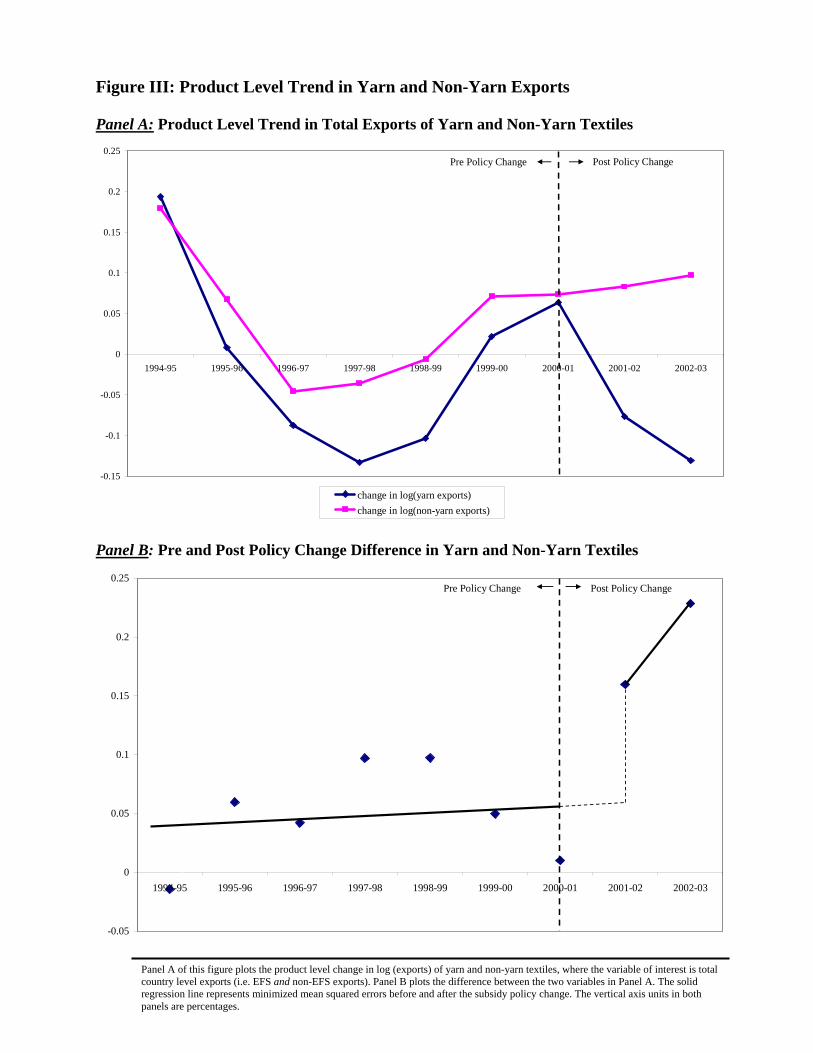
Figure III: Product Level Trend in Yarn and Non-Yarn Exports Panel A: Product Level Trend in Total Exports of Yarn and Non-Yarn Textiles
-0.15
-0.1
-0.05
0
0.05
0.1
0.15
0.2
0.25
1994-95 1995-96 1996-97 1997-98 1998-99 1999-00 2000-01 2001-02 2002-03
change in log(yarn exports)change in log(non-yarn exports)
Pre Policy Change Post Policy Change
Panel B: Pre and Post Policy Change Difference in Yarn and Non-Yarn Textiles
-0.05
0
0.05
0.1
0.15
0.2
0.25
1994-95 1995-96 1996-97 1997-98 1998-99 1999-00 2000-01 2001-02 2002-03
Pre Policy Change Post Policy Change
Panel A of this figure plots the product level change in log (exports) of yarn and non-yarn textiles, where the variable of interest is total country level exports (i.e. EFS and non-EFS exports). Panel B plots the difference between the two variables in Panel A. The solid regression line represents minimized mean squared errors before and after the subsidy policy change. The vertical axis units in both panels are percentages.

Figure IV: Yarn Ratio Density Panel A: Full Sample
01
23
4D
ensi
ty
0 .2 .4 .6 .8 1ty_Yarn Ratio
Panel B: Conditional on being a Yarn Exporter
0.5
11.
5D
ensi
ty
0 .5 1ty_Yarn Ratio
Panel A of this figure plots the density of firm level Yarn Ratio in the pre period, where Yarn Ratio is the ratio of a firm’s yarn exports to its total (yarn + non-yarn) exports in the pre-period. Panel B plots the density restricted to firms that export yarn. The horizontal axis represents Yarn Ratio.

Figure V: Year-by-Year Regression Coefficients for Total Loans and Exports
-0.35-0.3
-0.25-0.2
-0.15-0.1
-0.050
0.050.1
0.150.2
199899 199900 200001 200102 200203
Total LoansExports
Figure V: Year-by-Year Regression Coefficients for Total Loans and Exports
Post Policy ChangePre Policy Change
This figure plots the year-by-year regression coefficients, tβ and jβ respectively, resulting from the following regressions for total loans and exports:
ittittiit YarnRatioLoans TotalLog εδβδα +++= )*.()( where iα and tδ are firm and year dummies respectively, and each tβ is the coefficient of the interaction between Yarn Ratio and the corresponding year
dummy. itε is the error term.
iijiji YarnRatioExportsLogExportsLog εβττ ++=+ .)()( ,, where τ refers to year 1 in the sample (i.e. 1998-99), and j=1,2,3,4 refers to all four subsequent years. jβ is the coefficient on Yarn Ratio for each jth cross-
sectional regression. iε is the error term.

Figure VI: Time Trend for Real Domestic Prices
0
200
400
600
800
1000
1200
1990-91 1991-92 1992-93 1993-94 1994-95 1995-96 1996-97 1997-98 1998-99 1999-00 2000-01 2001-02 2002-03
Real Cotton Price (per 10 kg)Real Yarn Price (per 10 kg)
This figure plots the time-series trend in real prices of yarn and raw cotton, where raw cotton is an input into yarn production. Real prices are calculated by normalizing all year values to 2000-01 prices using the Consumer Price Index for Pakistan.

Figure VIII: Do Banks Screen Out Defaulting Firms?
-0.8
-0.7
-0.6
-0.5
-0.4
-0.3
-0.2
-0.1
0199899 199900 200001 200102 200203
This figure tests if firms that default on their loans in the first sample period (1998-99) are awarded less loans in the following years. The figure plots the regression coefficients, tβ , from the following regression:
ittittiit DefaultTotalLoansLog εδβδα +++= )*.()( where iα and tδ are firm and year dummies, and Default is a firm-level dummy=1 if firms have non-zero defaults on their loans in 1998-
99, and =0 otherwise. tβ are the coefficients on the interaction of Default and year dummies.
Figure VII: Do Banks Screen Out Defaulting Firms?

(1)All SectorsYears Covered 1998-2003Total no. of Unique Loans 97,937 % Loans to Textile Sector 51.73%
Textile SectorNo. of Unique Loans 50,661No. of Unique Firms 1,120No. of Matched Firms* 978
(1) (2) (3) (4) (5)
Mean Std. Dev. Min Max # of loansLoan Amount (Rs.)
Other Textiles 2,509,215 4,070,170 100,000 172,000,000 27,100 Yarn 4,693,878 7,798,886 100,000 110,000,000 8,948
All Textiles 3,051,882 5,336,440 100,000 172,000,000 36,048
Shipment Value (Rs.)Other Textiles 3,090,001 4,364,866 104,701 173,000,000 27,116
Yarn 5,408,996 8,178,908 108,633 116,000,000 8,951 All Textiles 3,666,021 5,654,027 104,701 173,000,000 36,067
Net Fine (Rs.) Other Textiles 184,996 1,025,954 300 20,000,000 750
Yarn 317,847 1,609,918 480 20,000,000 218 All Textiles 214,915 1,183,213 300 20,000,000 968
Net Fine/Shipment Value RatioOther Textiles 0.151 0.735 0.00004 6.714 0.027
Yarn 0.109 0.617 0.00002 7.656 0.024All Textiles 0.142 0.71 0.00002 7.656 0.027
Figures are in Rs. and correspond to loan-level observations in the pre-period (1998-99 to 2000-01).
Table I (b)EFS Data Summary Statistics
Table I (a)EFS Data Description
*This refers to the number of firms successfully matched with the Total Loans database.

Mean Std. Dev.25th
Percentile50th
Percentile75th
Percentile80th
Percentile
Panel A: Total Loans Data (Rs. 000)
Total Working Capital Loans 131,569 776,007 4,604 18,779 104,210 150,681Total Fixed Investment Loans 97,656 228,093 2,179 15,591 114,456 153,216Default Rate (%) 10.3 27.2 0 0 0 2.1
Mean Std. Dev.25th
Percentile50th
Percentile75th
Percentile80th
Percentile
Panel B: Corporate Accounts Data (Rs. 000)Total Assets 771,961 1,776,424 233,200 483,803 811,521 881,232Equity 149,009 624,848 48,361 88,850 134,800 151,400Capital Expenditure 67,877 197,970 3,082 14,243 57,324 77,552Total Sales 976,818 1,523,457 371,453 642,600 1,083,500 1,306,460Profits 27,122 224,832 -7,797 15,058 54,900 70,656
Summary Statistics for Firm-Level Total Loans and Corporate Accounts DataTable I (c)
The total loans data in Panel A comprises all EFS firms, publicly listed and private. The corporate accounts data in Panel B comprises only publicly listed firms. Figures are in Rs. thousands (000) and correspond to firm-level observations in the pre-period (1998-99 to 2000-01).

(1) (2) (3)Log of Total Working
Capital LoansLog of Total Working
Capital Loans Exit?Yarn Dummy * Post -0.187***
(0.060)Yarn Ratio * Post -0.224*** 0.096***
(0.074) (0.029)
Firm FEs YES YES YESYear FEs YES YES YESObservations 4299 4299 4890R-squared 0.922 0.922 0.558
(1) (2) (3)
Log of Post Period Exports
Log of Post Period Exports
Log of Post Period Exports
Yarn Dummy -0.164***(0.049)
Yarn Ratio -0.315*** -0.297***(0.063) (0.074)
Log of Pre Period Average Exports 0.956*** 0.952*** 0.956***(0.016) (0.015) (0.018)
Year FEs YES YES YESObservations 2240 2240 1803R-squared 0.708 0.710 0.686
Table II (b) Effect of EFS Eligibility Change on Export Output
Table II (a) Are Yarn Firms Able to Substitute to Non-Program Loans?
Robust standard errors, clustered at firm-level, are reported in parentheses."Yarn Ratio" refers to the ratio of a firm's yarn exports to its total (yarn and non-yarn) exports in the pre-period under EFS. The pre-period consists of 3 years, 1998-99 to 2000-01, and the post-period consists of 2 years, 2001-02 and 2002-03. In Columns (1) and (2), data is restricted to intensive margin firms. Column (3) reports regression results on the entire sample, where Exit is a dummy=1 if a firm stops borrowing from banks in the post-period, and =0 otherwise. * significant at 10%; ** significant at 5%; *** significant at 1%
Robust standard errors, clustered at firm-level, are reported in parentheses. "Yarn Ratio" refers to the ratio of a firm's yarn exports to its total (yarn and non-yarn) exports in the pre-period under EFS. The pre-period consists of 3 years, 1998-99 to 2000-01, and the post-period consists of 2 years, 2001-02 and 2002-03. All loans in the pre-period (1998-99 to 2000-01) are averaged at the firm level. The regressions are run on all post periods (2001-02 and 2002-03), and include time dummies for the two post periods. In Column (3), data is restricted to intensive margin firms. * significant at 10%; ** significant at 5%; *** significant at 1%

(1) (2)Mean Std. Dev.
Publicly Listed FirmsExport Value (Rs. 000) 176,145 312,627
EFS Loan Amount (Rs. 000) 152,660 276,781Total Working Capital Loan Amount (Rs. 000) 402,252 977,378
Ratio of EFS to Total Working Capital Loans 0.46 0.37Default Rate (%) 5.32 14.54No. of Banks 7.68 7.12
Yarn Ratio 0.50 0.41Yarn Ratio | Yarn 0.67 0.34
No. of Firms 158
Privately Owned FirmsExport Value (Rs. 000) 45,474 101,251
EFS Loan Amount (Rs. 000) 36,542 82,738Total Working Capital Loan Amount (Rs. 000) 53,911 213,837
Ratio of EFS to Total Working Capital Loans 0.65 0.36Default Rate (%) 7.61 24.34No. of Banks 2.19 2.67
Yarn Ratio 0.18 0.32Yarn Ratio | Yarn 0.45 0.38
No. of Firms 820
Table III (a) Comparing Publicly Listed and Privately Owned Firms
This table presents summary statistics for the three sample years in the pre-policy change period (1998-99 - 2000-01), separately for publicly listed firms and private firms. "Yarn Ratio | Yarn" refers to the average "Yarn Ratio" only for firms that export yarn; all non-yarn firms are excluded.

(1) (2) (3) (4) (5) (6) (7) (8)
Yarn Ratio * Post -0.244** -0.366*** -0.274** -0.233**(0.104) (0.119) (0.117) (0.117)
Yarn Ratio * Post * Listed 0.173** 0.157** 0.149* 0.056(0.078) (0.080) (0.083) (0.092)
Yarn Ratio * Post * Large 0.281** 0.216* 0.207*(0.118) (0.115) (0.114)
Yarn Ratio * Post * Subsidy Dependence -0.136* -0.197**(0.079) (0.084)
Yarn Ratio * Post * Subsidy Dependence * Listed 0.314***
(0.122)
Yarn Ratio -0.289*** -0.387*** -0.299*** -0.254**(0.090) (0.098) (0.104) (0.107)
Yarn Ratio * Listed 0.286* 0.277* 0.272* 0.101(0.155) (0.156) (0.159) (0.161)
Yarn Ratio * Large 0.322* 0.278* 0.234**(0.174) (0.167) (0.104)
Yarn Ratio * Subsidy Dependence -0.201** -0.263**(0.094) (0.103)
Yarn Ratio * Subsidy Dependence * Listed 0.389***(0.131)
Log of Pre Period Average Exports 0.961*** 0.980*** 0.913*** 0.908***(0.019) (0.020) (0.022) (0.022)
Firm FEs YES YES YES YESYear FEs YES YES YES YES YES YES YES YES
Observations 4299 4299 4299 4299 1803 1803 1803 1803R-squared 0.922 0.924 0.923 0.923 0.687 0.692 0.708 0.708
Log of Total Working Capital Loans
Testing for Heterogeneous Effects: Publicly Listed vs. Privately Owned FirmsTable III (b)
Log of Post Period Exports
Robust standard errors, clustered at firm-level, are reported in parentheses. "Yarn Ratio" refers to the ratio of a firm's yarn exports to its total (yarn and non-yarn) exports in the pre-period under EFS. The pre-period consists of 3 years, 1998-99 to 2000-01, and the post-period consists of 2 years, 2001-02 and 2002-03. "Listed" is a dummy=1 for firms that are publicly listed in the pre-period; "Large" is a dummy =1 for firms in the top quartile of the size distribution in the pre-period; "Subsidy Dependence" is the ratio of EFS loans to total working capital loans for each firm in the pre-period. The Loan regressions in Columns (1) - (4) are run on a panel of 5 years, and include all interactions of regressors with year dummies. For Export regressions in Columns (5)-(8), all loans in the pre-period (1998-99 to 2000-01) are averaged at the firm level and the regressions are run on all post periods (2001-02 and 2002-03). These regressions also include all regressors independently and interacted with year dummies for the two post periods. The sample in all columns is restricted to intensive margin firms. * significant at 10%; ** significant at 5%; *** significant at 1%

(1) (2)Mean Std. Dev.
Firms in Group NetworksExport Value (Rs. 000) 68,311 131,467
EFS Loan Amount (Rs. 000) 55,291 103,566Total Working Capital Loan Amount (Rs. 000) 79,987 193,159
Ratio of EFS to Total Working Capital Loans 0.63 0.40Default Rate (%) 7.69 22.38No. of Banks 3.98 4.72
Yarn Ratio 0.19 0.34Yarn Ratio | Yarn 0.45 0.39
No. of Firms 328
Firms not in Group NetworksExport Value (Rs. 000) 33,919 79,448
EFS Loan Amount (Rs. 000) 27,045 68,091Total Working Capital Loan Amount (Rs. 000) 31,483 99,642
Ratio of EFS to Total Working Capital Loans 0.81 0.31Default Rate (%) 8.91 25.01No. of Banks 1.70 1.19
Yarn Ratio 0.16 0.31Yarn Ratio | Yarn 0.44 0.37
No. of Firms 492
Table IV (a) Private Firm Heterogeneity: Comparing In-Network and Out-of-Network Firms
This table presents summary statistics for the three sample years in the pre-policy change period (1998-99 - 2000-01), separately for privately owned firms that are part of a group network and those that are not. A firm is "In-Network" if it has a board of director in common with at least 5 other firms. "Yarn Ratio | Yarn" refers to the average "Yarn Ratio" only for firms that export yarn; all non-yarn firms are excluded.

(1) (2) (3) (4) (5) (6) (7) (8)
Yarn Ratio * Post -0.479*** -0.397*** -0.369*** -0.492***(0.140) (0.142) (0.093) (0.110)
Yarn Ratio * Post * In Group Network 0.502** 0.459**(0.211) (0.223)
Yarn Ratio * Post * Multiple Lenders 0.401* 0.362*(0.209) (0.205)
Yarn Ratio * Post * Large 0.304* 0.276(0.181) (0.233)
Yarn Ratio -0.433*** -0.447*** -0.385*** -0.542***(0.111) (0.140) (0.103) (0.119)
Yarn Ratio * In Group Network 0.385*** 0.362**(0.189) (0.179)
Yarn Ratio * Multiple Lenders 0.481** 0.365*(0.209) (0.215)
Yarn Ratio * Large 0.355** 0.282*(0.147) (0.168)
Log of Pre Period Average Exports 0.951*** 0.960*** 0.961*** 0.970***(0.023) (0.022) (0.023) (0.023)
Firm FEs YES YES YES YES
Year FEs YES YES YES YES YES YES YES YES
Observations 3579 3579 3579 3579 1498 1498 1498 1498
R-squared 0.893 0.893 0.893 0.894 0.632 0.641 0.633 0.645
Table IV (b)Private Firm Heterogeneity: Testing for Characteristics of Financial Constraints
Log of Total Working Capital Loans Log of Post Period Exports
Robust standard errors, clustered at firm-level, are reported in parentheses. "Yarn Ratio" refers to the ratio of a firm's yarn exports to its total (yarn and non-yarn) exports in the pre-period under EFS. The pre-period consists of 3 years, 1998-99 to 2000-01, and the post-period consists of 2 years, 2001-02 and 2002-03. "In Group Network" is a dummy=1 for firms that have a director in common with at least 5 other firms in the pre-period; "Multiple Lenders" is a dummy=1 for firms that borrow from more than one bank in the pre-period; "Large" is a dummy =1 for firms in the top quartile of the size distribution in the pre-period. The Loan regressions in Columns (1) - (4) are run on a panel of 5 years, and include all interactions of regressors with year dummies. For Export regressions in Columns (5)-(8), all loans in the pre-period (1998-99 to 2000-01) are averaged at the firm level and the regressions are run on all post periods (2001-02 and 2002-03). These regressions also include all regressors independently and interacted with year dummies for the two post periods. The sample in all columns is restricted to privately owned intensive margin firms. * significant at 10%; ** significant at 5%; *** significant at 1%

(1) (2) (3) (4) (5) (6)
Log of Fixed Assets
Log of Total Assets CAPX Equity
Log of Total Sales Profits
Panel A: Balance Sheet Changes
Yarn Ratio * Post 0.07 -0.094 -0.13 -0.081 -0.085 -0.171*(0.094) (0.175) (0.103) (0.155) (0.103) (0.099)
Firm FEs YES YES YES YES YES YESYear FEs YES YES YES YES YES YESAssets * Post YES YES YES YESObservations 691 691 383 691 691 691R-squared 0.93 0.937 0.532 0.875 0.947 0.564
(1) (2) (3)
Equity ShareTrade Credit
ShareBank Debt
Share
Panel B: Capital Structure Changes
Yarn Ratio * Post -0.025 0.013 0.038(0.036) (0.037) (0.035)
Firm FEs YES YES YESYear FEs YES YES YESAssets * Post YES YES YESObservations 691 227 691R-squared 0.735 0.521 0.816
Table VBalance Sheet and Capital Structure Changes for Publicly Listed Firms
Robust standard errors, clustered at firm-level, are reported in parentheses. "Yarn Ratio" refers to the ratio of a firm's yarn exports to its total (yarn and non-yarn) exports in the pre-period under EFS. The pre-period consists of 3 years, 1998-99 to 2000-01, and the post-period consists of 2 years, 2001-02 and 2002-03. In Panel A, dependent variables in Columns (3), (4), and (6) are normalized by pre-period average total assets. In Panel B, "Equity Share" refers to the share of equity in total capital (equity + trade credit + bank debt). The same definition applies for "Trade Credit Share" and "Bank Debt Share". "Assets * Post" is an interaction term between "Log of Pre-period Total Assets" and the "Post" dummy. Data is for publicly listed firms only. * significant at 10%; ** significant at 5%; *** significant at 1%

Table VIAnalysis of the Profit and Loss Account
(1) (2) (3) (4)
Mean Std. Dev. Min Max
Panel A: Summary Statistics
Manufacturing Costs (Rs. Millions) 827.00 1200.00 5.51 14300.00Financial Charges (Rs. Millions) 72.50 210.00 0.06 3220.00Administrative & Selling Expenses (Rs. Millions) 45.50 97.30 0.03 1070.00Taxes (Rs. Millions) 11.30 17.90 0.07 149.00Total Cost (Rs. Millions) 841.00 1400.00 6.32 17500.00Interest Exps / Total Cost 0.13 0.19 0.02 0.84Total Sales (Rs. Millions) 977.00 1520.00 6.66 16500.00Net Profit (Rs. Millions) 27.10 225.00 -8.13 1200.00
(1) (2) (3) (4)Log of Manf.
CostsLog of Fin.
CostsLog of Admin.
CostsLog of Wages
per Emp.
Panel B: Where is the Cost Adjustment Coming From?Yarn Ratio * Post 0.089 0.355* -0.065 -0.052
(0.117) (0.210) (0.104) (0.170)
Firm FEs YES YES YES YESYear FEs YES YES YES YESAssets * Post YES YES YES YESObservations 691 691 691 691R-squared 0.947 0.885 0.972 0.795Robust standard errors, clustered at firm-level, are reported in parentheses. "Yarn Ratio" refers to the ratio of a firm's yarn exports to its total (yarn and non-yarn) exports in the pre-period under EFS. The pre-period consists of 3 years, 1998-99 to 2000-01, and the post-period consists of 2 years, 2001-02 and 2002-03. In Panel B, "Log of Financial Costs" refers to the Log of interest expenses on bank debt. "Assets * Post" is an interaction term between "Log of Pre-period Total Assets" and the "Post" dummy. Data is for publicly listed firms only. * significant at 10%; ** significant at 5%; *** significant at 1%

Table VIIShort-Term vs. Long-Term Impact for Publicly Listed Firms
(1) (2) (3) (4) (5) (6) (7)
Log of Fixed Assets
Log of Total Assets
Long-Term Investments Equity Issued Dividends
Log of Total Sales Profits
Yarn Ratio * Post1 0.072 -0.099 -0.038 0.04 -0.019 -0.062 -0.171*(0.099) (0.173) (0.024) (0.081) (0.045) (0.105) (0.096)
Yarn Ratio * Post2 0.049 -0.04 -0.01 0.089 0.004 -0.035 -0.133(0.244) (0.231) (0.075) (0.129) (0.057) (0.182) (0.114)
Firm FEs YES YES YES YES YES YES YESYear FEs YES YES YES YES YES YES YESAssets * Post1 YES YES YES YES YESAssets * Post2 YES YES YES YES YESObservations 871 871 209 871 338 871 871R-squared 0.885 0.864 0.904 0.915 0.816 0.902 0.467Robust standard errors, clustered at firm-level, are reported in parentheses. "Yarn Ratio" refers to the ratio of a firm's yarn exports to its total (yarn and non-yarn) exports in the pre-period under EFS. The pre-period consists of 3 years, 1998-99 to 2000-01, and the post-period consists of 4 years, 2001-02 to 2004-05. "Post1" is a dummy=1 for only the two immediate post-periods, 2001-02 and 2002-3, and measures the short-term impact"Post2" is a dummy=1 for only the two final post periods, 2003-04 and 2004-05, and measures the long-term impact . Dependent variables in Columns (4), (5), and (7) are normalized by pre-period average total assets. "Assets * Post1" is an interaction term between "Log of Pre-period Total Assets" and the "Post1" dummy. "Assets * Post2" is an interaction term between "Log of Pre-period Total Assets" and the "Post2" dummy. Data is for publicly listed firms only. * significant at 10%; ** significant at 5%; *** significant at 1%
.

(1) (2)Log of Total Working
Capital LoansLog of Post Period
Exports
Yarn Ratio * Post -0.248**(0.107)
Yarn Ratio * Post * Listed 0.166**(0.082)
Yarn Ratio * Post * Productivity 0.047(0.081)
Yarn Ratio * Post * Productivity * Listed 0.095(0.099)
Yarn Ratio -0.293***(0.092)
Yarn Ratio * Listed 0.288*(0.159)
Yarn Ratio * Productivity 0.056(0.063)
Yarn Ratio * Productivity * Listed 0.154(0.117)
Log of Pre Period Average Exports 0.913***(0.022)
Firm FEs YESYear FEs YES YES
Observations 4299 1803R-squared 0.928 0.704
Does Export Productivity Matter?Table VIII
Robust standard errors, clustered at firm-level, are reported in parentheses. "Yarn Ratio" refers to the ratio of a firm's yarn exports to its total (yarn and non-yarn) exports in the pre-period under EFS. The pre-period consists of 3 years, 1998-99 to 2000-01, and the post-period consists of 2 years, 2001-02 and 2002-03. "Productivity" is log of the ratio of EFS exports to working capital loans for each firm in the pre-period. The Loan regression in Column (1) is run on a panel of 5 years, and includes all interactions of regressors with year dummies. For the Export regression in Column (2), all loans in the pre-period (1998-99 to 2000-01) are averaged at the firm level and the regression is run on all post periods (2001-02 and 2002-03). This regression also includes all regressors independently and interacted with year dummies for the two post periods. The sample in all columns is restricted to intensive margin firms. * significant at 10%; ** significant at 5%; *** significant at 1%

(1) (2) (3) (4) (5) (6)
Non-Yarn Textile Firms
Non-Textile Firms
All Sample Firms
Non-Yarn Textile Firms
Non-Textile Firms
All Sample Firms
(NonTextile=1) * Post 0.234* 0.261**(0.126) (0.127)
Post Dummy 0.042 0.242*** 0.064 0.288***(0.117) (0.063) (0.111) (0.059)
Firm FEs YES YES YES YES YES YESYear FEs YES YESObservations 1518 5170 6688 1518 5170 6688R-squared 0.809 0.854 0.845 0.797 0.845 0.836
Table IXIs There Cross-Industry Redistribution of EFS Funds?
Log of EFS Loans Log of EFS Exports
Robust standard errors, clustered at firm-level, are reported in parentheses. Data in all columns is restricted to non-textile firms and textile firms that are non-yarn (i.e. firms with yarn ratio =0). Columns 1 and 4 report results for non-yarn textile firms, while columns 2 and 5 report results for non-textile firms. "(NonTextile=1)" is a dummy = 1 if the firm is non-textile, and is = 0 if the firm is textile AND non-yarn. The pre-period consists of 3 years, 1998-99 to 2000-01, and the post-period consists of 2 years, 2001-02 and 2002-03. * significant at 10%; ** significant at 5%; *** significant at 1%

(1) (2)Log of Total Working
Capital LoansLog of Post Period
Exports
Yarn Ratio * Post -0.240**(0.119)
Yarn Ratio * Post * Listed 0.171**(0.084)
Pre-Default * Post -0.313***(0.081)
Pre-Default * Post * Listed 0.046(0.162)
Pre-Default * Post * Yarn Ratio 0.031(0.207)
Pre-Default * Post * Yarn Ratio * Listed 0.08(0.285)
Yarn Ratio -0.260**(0.104)
Yarn Ratio * Listed 0.249**(0.113)
Pre-Default -0.318***(0.087)
Pre-Default * Listed 0.079(0.182)
Yarn Ratio * Pre-Default 0.013(0.212)
Yarn Ratio * Pre-Default * Listed 0.13(0.333)
Log of Pre Period Average Exports 0.961***(0.021)
Firm FEs YESYear FEs YES YES
Observations 4299 1803R-squared 0.919 0.677
Do Banks Screen Out Defaulting Firms?Table X
Robust standard errors, clustered at firm-level, are reported in parentheses. "Yarn Ratio" refers to the ratio of a firm's yarn exports to its total (yarn and non-yarn) exports in the pre-period under EFS. The pre-period consists of 3 years, 1998-99 to 2000-01, and the post-period consists of 2 years, 2001-02 and 2002-03. "Pre-Default" is a dummy =1 if a firm has positive default on its loans in the pre-period. The Loan regression in Column (1) is run on a panel of 5 years, and includes all interactions of regressors with year dummies. For the Export regression in Column (2), all loans in the pre-period (1998-99 to 2000-01) are averaged at the firm level and the regression is run on all post periods (2001-02 and 2002-03). This regression also includes all regressors independently and interacted with year dummies for the two post periods. The sample in all columns is restricted to intensive margin firms. * significant at 10%; ** significant at 5%; *** significant at 1%