export diversification and output volatility: comparative ... · export diversification and output...

1

Export diversification and output volatility: comparative firm-level

evidence

Urška Čede1, Bogdan Chiriacescu

2, Péter Harasztosi

3, Tibor Lalinsky

4, Jaanika Meriküll

5

22.05.2015

Abstract: The literature shows that openness to trade improves long-term growth but equally

that it may increase exposure to high volatility. In this vein, our paper investigates whether

diversification at the firm level lowers the output volatility of the firms, using data for

Estonia, Hungary, Romania, Slovakia and Slovenia over the last boom-bust cycle. The

instrumental variable technique is used to estimate the effect of endogenously treated

diversification on the volatility of sales growth. The results show that the effect of export

diversification on output volatility is statistically significant and economically large.

Exporters that are more diversified by one standard deviation experience smaller output

volatility of one fifth to four fifth of a standard deviation. The effect of the diversification in

products is somewhat larger than the effect of diversification in destination markets, and the

diversification effect decreased during the Great Recession. This decrease is related to the

large and correlated negative shocks in all destination markets.

Keywords: export diversification, volatility of sales, business cycle, Europe

JEL codes: F14, F43, O57

Acknowledgement

The authors are grateful to Luca David Opromolla, Karsten Staehr, participants of the

presentations held in Bratislava, Frankfurt and Brno for their insightful comments; Robin

Hazlehurst for excellent language editing, and for the financial support from Estonian

Research Council Grant IUT20-49.

1 Bank of Slovenia; Slovenska 35, 1505 Ljubljana, Slovenia; [email protected].

2 National Bank of Romania; 25 Lipscani Street, Sector 3, 030031 Bucharest, Romania;

[email protected]. 3 The Central Bank of Hungary; 1054 Szabadság tér 8/9, 1850 Budapest, Hungary; [email protected].

4 National Bank of Slovakia; Imricha Karvasa 1, 813 25 Bratislava, Slovakia, [email protected].

5 Bank of Estonia and University of Tartu; Estonia pst 13, 15095 Tallinn, Estonia;

[email protected].

2

1. Introduction

Since the influential work by Ramey and Ramey (1995), many empirical studies have been

concerned that higher volatility can lead to lower growth. In the global economy, the issue

often translates to the view in academic and policy discussions that openness to international

trade leads to higher GDP volatility. This view hinges on the two assumptions that openness

to trade increases specialisation and that GDP volatility is dominantly led by sector specific

shocks. Indeed, Bejan (2006) and Haddad et al. (2013) show that openness to trade does not

necessarily increase growth volatility if the export basket is diversified.

The second assumption was called into question by several empirical studies (e.g. Koren and

Tenreyro (2007)) showing that country-specific shocks, shocks common to all sectors in a

given country, are at least as important as sector-specific shocks. Subsequently, Caselli et al.

(2012) highlighted how the sign and size of the effect of exporting on GDP volatility depends

on the volatility of shocks in the trading partners and the correlation between those and the

shock affecting the domestic economy. In particular, higher volatility arises when foreign

markets are more volatile than the domestic market and when there is a high correlation

between country-specific shocks.

While macro level studies are more abundant, empirical evidence on exporting and volatility

at the firm level is scarce and inconclusive. In this paper we study the relationship between

export diversification and output volatility at the firm level using comparative micro-data

from five countries. Our contribution to the literature is threefold. First, unlike the previous

studies we address the endogeneity of diversification in the volatility equation. Second, we

apply an identical methodology to large representative firm-level databases from five

countries. Data for manufacturing firms from Estonia, Hungary, Romania, Slovakia and

Slovenia have been used. These five countries form a good case study because they have all

experienced fast growth and high volatility, but they have different diversification patterns.

Third, we test whether the effect of diversification on volatility has changed over the business

cycle. The time period analysed covers the last business cycle of 2004-2012 for most of the

sample countries. There are rich dynamics in firm sales during this time, making it possible to

study the effect of diversification on volatility over the boom and bust period.

Our results show that export diversification has a strong negative effect on firm-level output

volatility, meaning that exporting more types of products or serving more markets leads to

higher stability for firm sales. Exporters that are more diversified by one standard deviation

have lower volatility by one fifth to four fifth of a standard deviation. The diversification

effects are the strongest in Romania and the weakest in Hungary. There is also evidence that

the diversification of products has a stronger effect on volatility than the diversification of

destination markets, and that the diversification effect is weaker for larger firms. Our results

are robust to the different sets of instruments applied. The second result from our study is that

the negative effect of diversification on volatility decreased during the recession that followed

the global financial crisis. This result is most likely related to the common negative shock that

occurred in all destination markets during the recession.

Our paper adds to the growing evidence on the granular nature of aggregate growth volatility,

e.g., Gabaix (2011), which has shed light on the importance of the firm heterogeneity that lies

behind the macro aggregates. In this vein, di Giovanni et al. (2014) analyse the link between

export diversification and volatility by applying the Melitz (2003) model of heterogeneous

firms with export entry costs. Di Giovanni et al. (2014) study the role of firms in the business

3

cycle by disentangling the role of country, sector and firm-specific shocks. They argue that

synchronisation of the business cycles of destination countries, or cross-sector correlation due

to input-output linkages, increases aggregate volatility, whereas diversification across markets

and sectors reduces the aggregate volatility. Similarly, firm-level co-movement of sales and

the higher volatility of larger firms are factors in the higher contributions by firm-specific

shocks to aggregate volatility. Kramarz et al. (2014) find similar results by examining

networks.

Our paper is more closely linked to the empirical studies, although the evidence on the

contribution of firm-level openness is still ambiguous. On the one hand, Buch et al. (2009)

argue that exporters have lower output volatility and that this effect stems mostly from the

extensive and not from the intensive margin. On the other hand, Vannoorenberghe (2012)

finds that a large export share is related to lower export volatility. He also shows that the sales

to domestic and foreign markets are negatively correlated, indicating the simultaneity of the

diversification decision and volatility. Evidence also points to the importance of firm size.

Vannoorenberghe et al. (2014) study the effect of export diversification on volatility and find

the pattern to be different for small and large firms; export diversification is related to higher

volatility in small firms and to lower volatility in large firms. The main channel behind high

export volatility for small firms is that smaller firms occasionally export to new markets.

The paper is organised as follows. The next section provides a background for the study by

presenting a theoretical model motivating the empirical specification and the characteristics of

sample countries. The third section describes the empirical specification and the data. The

fourth section presents the results together with a number of robustness tests, and the last

section summarises the results.

2. Background of the study

2.1 Theoretical setting

This section presents a simple theoretical model to show how various shocks can affect firms’

volatility of output. We build on Buch et al. (2009), who consider a neoclassical model where

firms maximise profits in an exogenous environment. Firm i produces output Yit using the

Cobb-Douglas production function with constant returns to scale and with domestic labour Lit

and domestic capital Kit as inputs:

𝑌𝑖𝑡 = 𝐴𝑖𝑡𝐿𝑖𝑡𝛼 𝐾𝑖𝑡

1−𝛼 (1)

where α denotes the labour share and Ait is the parameter capturing technology. Unlike in

Buch et al. (2009) we allow productivity shocks to be firm-specific and not common to all the

firms in the country. This extension does not change the main outcome of the theoretical

model, but is in line with our empirical specification where total factor productivity is

measured at the firm level. The firm sells λi share of output domestically and exports the rest.

The firm can sell to one or more foreign markets k and the sum of each foreign market share,

∑ 𝜆𝑘𝑖∗𝐾

𝑘=1 , equals 1-λi. Firm profits are defined as:

𝜋𝑖𝑡 = [𝑝𝑡𝜆𝑖 + ∑ (𝑝𝑘𝑡∗ − 𝑐𝑘𝑡)𝜆𝑘𝑖

∗𝐾𝑘=1 ]𝑌𝑖𝑡 − 𝑤𝑡𝐿𝑖𝑡 − 𝑟𝑡𝐾𝑖𝑡 (2)

4

The prices of the product in the domestic market pt and in foreign markets 𝑝𝑘𝑡∗ are given to the

firm and so is the exporting cost per unit of product for each destination market, ckt. The firm

finds the optimal demand for labour given that the market shares, λi and 𝜆𝑘𝑖∗ , and capital, Kit,

are fixed in the short run. Taking the first-order condition from (2) and solving for labour

yields:

𝐿𝑖𝑡𝐷 = (

𝑤𝑡

[𝑝𝑡𝜆𝑖+∑ (𝑝𝑘𝑡∗ −𝑐𝑘)𝜆𝑘𝑖

∗𝐾𝑘=1 ]𝛼𝐴𝑖𝑡

)

1

𝛼−1= (

𝑤𝑡

𝑑𝑖𝑡𝛼𝐴𝑖𝑡)

−𝜂𝐷

(3)

where 𝑑𝑖𝑡 = [𝑝𝑡𝜆𝑖 + ∑ (𝑝𝑘𝑡∗ − 𝑐𝑘)𝜆𝑘𝑖

∗𝐾𝑘=1 ] denotes demand conditions in domestic and foreign

markets and -ηD = 1/(α-1) denotes the value of the labour demand elasticity. The labour

supply is given by 𝐿𝑡𝑆 = 𝑤𝑡

𝜂𝑆

, and then solving for equilibrium wages and equilibrium

employment gives 𝐿 = (𝑑𝛼𝐴)𝜂𝐷𝜂𝑆

𝜂𝐷+𝜂𝑆. Substituting optimal demand for labour in the production

function and taking logarithms gives:

𝑙𝑛�̅� = 𝛽0 + 𝛽1𝑙𝑛�̅� + 𝛽2𝑙𝑛�̅� + 𝛽3𝑙𝑛�̅� (4)

where 𝛽0 = 𝛼[𝜂𝐷𝜂𝑆/(𝜂𝐷 + 𝜂𝑆)]𝑙𝑛𝛼,

𝛽1 = 1 + 𝛼[𝜂𝐷𝜂𝑆/(𝜂𝐷 + 𝜂𝑆)], 𝛽2 = 𝛼[𝜂𝐷𝜂𝑆/(𝜂𝐷 + 𝜂𝑆)], 𝛽3 = 1 − 𝛼.

Variables with bars denote equilibrium values. Given the state of equilibrium, summarised in

equation (4), let us assume the firm faces random technology, demand and capital cost shocks,

𝛾𝐴 , 𝛾𝑑 and 𝛾𝐾 respectively. The time subscripts are suppressed from here on. Let us define

these shocks as 𝐴 = �̅�𝑒𝛾𝐴, 𝑑 = �̅�𝑒𝛾𝑑 = �̅�𝑒𝛾𝑝𝜆+∑ 𝛾𝑝𝑘

∗ −𝑐𝑘𝜆𝑘

∗𝑘

, and 𝐾 = �̅�𝑒𝛾𝐾 , where the demand

shock depends on the domestic and foreign demand shocks. The firm-specific shocks to A and

K are not correlated with each other or with the demand shock 𝜌(𝛾𝑑, 𝛾𝐴) = 0, 𝜌(𝛾𝑑, 𝛾𝐾) = 0,𝜌(𝛾𝐴, 𝛾𝐾) = 0, while the demand shocks of production markets can be correlated, but are not

perfectly correlated −1 < |𝜌(𝛾𝑝, 𝛾𝑝𝑘∗ )| < 1 for every foreign market k and −1 <

|𝜌 (𝛾𝑝𝑗∗ , 𝛾𝑝𝑘

∗ )| < 1 for every foreign market k ≠ j. The output with random shocks is given by:

𝑌 = exp (𝛽0 + 𝛽1 (ln(�̅�) + 𝛾𝐴) + 𝛽2(ln(�̅�) + 𝛾𝑑) + 𝛽3(ln (�̅�) + 𝛾𝐾)) (5)

and deriving the respective expressions of output with random shocks over the equilibrium

output, we obtain the following results for output growth:

ln (𝑌

�̅�) = 𝛽0 + 𝛽1 (ln(�̅�) + 𝛾𝐴) + 𝛽2(ln(�̅�) + 𝛾𝑑) + 𝛽3(ln (�̅�) + 𝛾𝐾) − (𝛽0 + 𝛽1ln (�̅�) +

𝛽2ln (�̅�) + 𝛽3ln (�̅�)) = 𝛽1𝛾𝐴 + 𝛽2𝛾𝑑 + 𝛽3𝛾𝐾 (6)

The variance of the output growth is then given by:

5

𝑉𝑎𝑟 (𝑙𝑛 (�̂�

𝑌)) = 𝛽1

2𝑉𝑎𝑟(𝛾𝐴) + 𝛽22 [𝜆2𝑉𝑎𝑟(𝛾𝑝) + ∑ 𝜆𝑘

∗ 2𝑉𝑎𝑟(𝛾𝑝𝑘

∗ )𝑘

] + 𝛽32𝑉𝑎𝑟(𝛾𝑘)

+ 𝛽22 [∑ 𝜆𝜆𝑘

∗

𝑘𝐶𝑜𝑣(𝛾𝑝, 𝛾𝑝𝑘

∗ ) + ∑ 𝜆𝑘∗ 𝜆𝑗

∗

𝑘≠𝑗𝐶𝑜𝑣(𝛾𝑝𝑘

∗ , 𝛾𝑝𝑗∗)]

(7)

If a firm is producing for one market only, be it domestic or foreign, the variance of output

depends on three components: variance of productivity shocks, variance of demand shocks in

the market, and variance of shocks to capital. If a firm is producing for more than one market,

more than three components enter the output volatility equation, and this case adds variance to

the demand shocks in all the markets and the covariance between the demand shocks for all

the markets. Each additional market decreases output volatility because of the diversification

effect in the covariance terms, but can increase volatility because of the high variance of

demand shocks in additional markets.

The relationship between diversification of markets and volatility can be positive or negative,

depending on the volatility of the markets served by a firm and the covariance of shocks

between the markets. We cannot disentangle the diversification and composition effects

empirically, but these mechanisms help us to understand and explain the effect of

diversification on volatility in the empirical section.

2.2. Volatility and openness at the country level

There are a large number of studies examining the link between openness and volatility using

industry or country-level data. The main mechanism behind the positive relationship between

openness and volatility is claimed to be more specialisation accompanied by openness. Rodrik

(1998) argues that trade reduces aggregate risk for a country as the world market is less

volatile than a single economy, but it also increases the specialisation that leads to

concentration of products and increases aggregate risks. He shows that product concentration

is positively correlated with growth volatility. Di Giovanni and Levchenko (2009) show that

industries more open to trade have higher volatility, but weaker correlation between industry

growth and aggregate growth. They show that the main mechanism behind the positive

correlation of openness and volatility is the higher specialisation of more open countries.

Haddad et al. (2013) demonstrate that trade diversification alters the relationship between

openness and growth volatility. Very open economies have lower volatility when their exports

are diversified and the diversification of products has a stronger effect on volatility than the

diversification of markets.

In addition to the diversification effect, the smaller size of the domestic market and the

structure of exports towards less volatile markets can reduce the volatility from openness.

Caselli et al. (2012) develop a model where the effect of openness on volatility depends on the

size of the country, the variance of productivity shocks from other countries and the

covariance of domestic and foreign productivity shocks.

The following explanation provides a comparative background of the sample countries in

terms of openness and volatility. All the countries are small, open economies from the upper

middle and high-income group of countries according to the World Bank definition. The

countries share common institutional features as they were all part of the communist world

6

before the 1990s and switched to market economic reforms in the late 1980s or early 1990s.

Although the speed and scope of the reforms have been different, their current level of

institutional development is relatively similar. All these countries became WTO members in

the 1990s and EU members in 2004 or 2007, and by 2015 three of them had joined the euro

zone.6

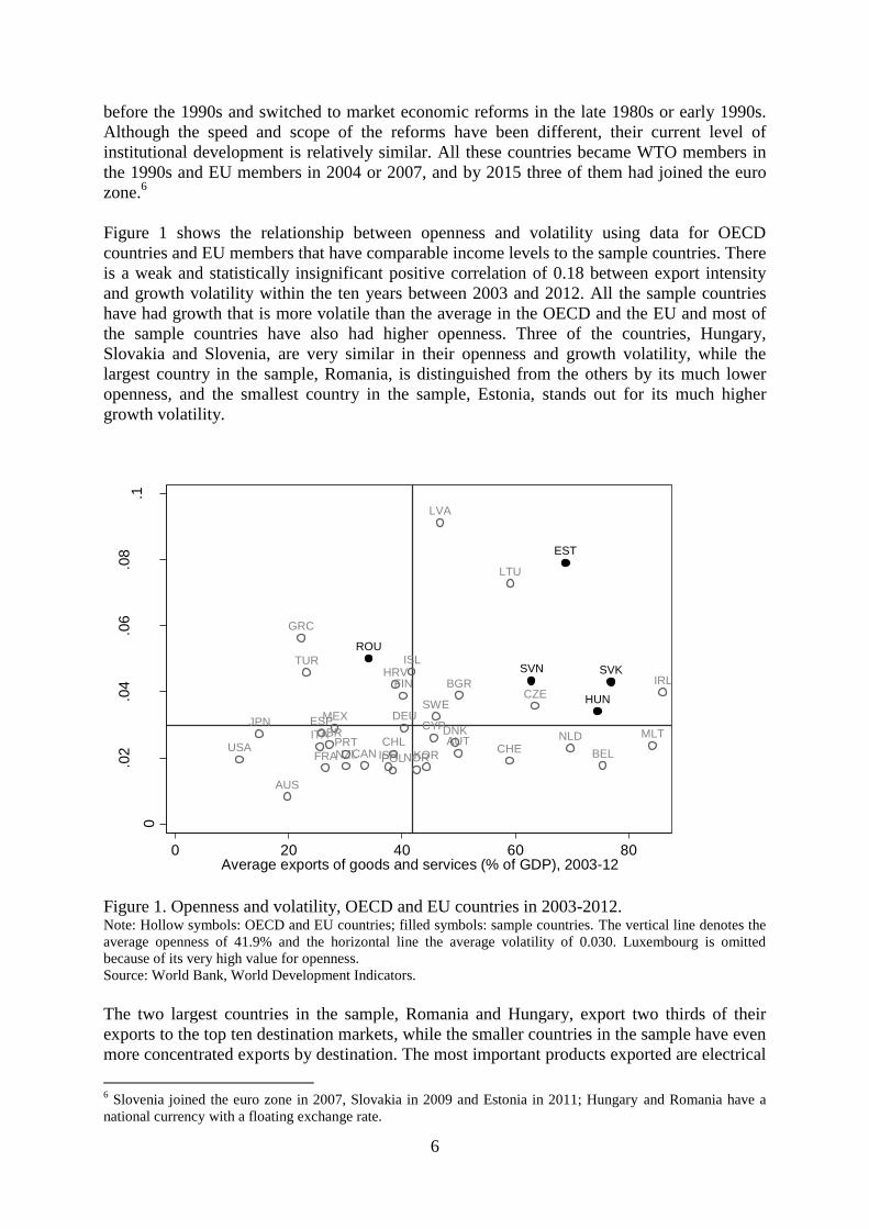
Figure 1 shows the relationship between openness and volatility using data for OECD

countries and EU members that have comparable income levels to the sample countries. There

is a weak and statistically insignificant positive correlation of 0.18 between export intensity

and growth volatility within the ten years between 2003 and 2012. All the sample countries

have had growth that is more volatile than the average in the OECD and the EU and most of

the sample countries have also had higher openness. Three of the countries, Hungary,

Slovakia and Slovenia, are very similar in their openness and growth volatility, while the

largest country in the sample, Romania, is distinguished from the others by its much lower

openness, and the smallest country in the sample, Estonia, stands out for its much higher

growth volatility.

Figure 1. Openness and volatility, OECD and EU countries in 2003-2012. Note: Hollow symbols: OECD and EU countries; filled symbols: sample countries. The vertical line denotes the

average openness of 41.9% and the horizontal line the average volatility of 0.030. Luxembourg is omitted

because of its very high value for openness.

Source: World Bank, World Development Indicators.

The two largest countries in the sample, Romania and Hungary, export two thirds of their

exports to the top ten destination markets, while the smaller countries in the sample have even

more concentrated exports by destination. The most important products exported are electrical

6 Slovenia joined the euro zone in 2007, Slovakia in 2009 and Estonia in 2011; Hungary and Romania have a

national currency with a floating exchange rate.

AUS

AUTBEL

BGR

CANCHL

HRV

CYP

CZE

DNK

FIN

FRA

DEU

GRC

ISL

IRL

ISR

ITAJPN

KOR

LVA

LTU

MLT

MEX

NLD

NZL NORPOL

PRT

ESP

SWE

CHE

TUR

GBR

USA

EST

HUN

ROU

SVKSVN

0

.02

.04

.06

.08

.1

St. d

ev. of G

DP

gro

wth

(an

nu

al)

, 20

03

-12

0 20 40 60 80Average exports of goods and services (% of GDP), 2003-12

7

machinery, vehicles and machinery, and mechanical applications, which make up more than

half of the exported products in Hungary and Slovakia and up to one third in Estonia and

Slovenia. Aggregated country-level data show that Slovakia and Estonia have the most

concentrated exports geographically and are exposed to concentrated risks from neighbouring

countries from Central Europe in Slovakia’s case or from Scandinavia and Russia for Estonia.

The covariance of shocks from destination markets is high as all the sample countries have a

strong focus on trade within the EU internal market and within the euro area. There is also a

strong common component of shocks from destination markets as the four Central European

sample countries have Germany as the main export destination that takes one fifth to one

quarter of their exports.

Given these findings it is suggested that the main factors behind higher volatility in the

sample countries are high export concentration and strong correlation of shocks across the

destination markets. The sample countries’ trade is also concentrated in products such as

transport equipment that are subject to high volatility from global sectoral shocks (see Koren

and Tenreyro (2007) for the list of sectors with more volatility from global sectoral shocks).

As a stabilising effect to foreign trade, the sample countries export mostly to high-income

countries with less volatile growth. There is some cross-country variation in the

diversification of exports in the sample countries, as the larger countries Romania and

Hungary are less exposed to volatility risk from concentrated exports. Last but not least, the

openness to trade is not necessarily the main factor behind high volatility as the domestic

markets have also been highly volatile during recent decades. The sample countries have

experienced a severe credit boom-bust cycle in asset prices (Bakker and Gulde (2010)).

3. Data and empirical specification

3.1. Empirical specification

There are two major challenges in our empirical specification. First, it is difficult to measure

volatility on firm-level data with yearly frequency. Given that firms in the sample countries

are relatively young, the panel specification where one observation in the time dimension

would be defined by a four or five-year interval would leave very many firms out of the panel.

This attrition problem is not an issue in country-level or industry-level studies, but is of high

relevance in firm-level studies. In order to keep as many firms as possible in the sample and

keep the sample representative of the population, we propose a specification based on a cross-

section where the volatility of output is computed over a four-year period.

The second challenge is related to the endogeneity of the diversification decision in the output

volatility equation. The endogeneity can originate from an omitted variable like an

unobserved productivity shock that affects both volatility and diversification or from the

simultaneity of volatility and diversification as firms can diversify their production in order to

reduce the expected volatility of output. We address the endogeneity issue by introducing a

specification that is strict in the chronological sequence of the diversification and volatility

decision, and by applying the instrumental variable technique. The volatility in the period

between time t+1 and time t+4 is dependent on the diversification decision in time t so that

the unobserved productivity shock from the same period cannot affect both diversification and

volatility. As the diversification decision in time t can still depend on the expected volatility,

the diversification is instrumented by firm characteristics related to the potential for

internationalisation such as firm size, age, export share and foreign ownership.

8

Given these concerns in the empirical specification, we cannot test the theoretical

specification in equation (8) empirically one to one, but we aim to model the effect of the

same variables as in equation (9) on output volatility. The following simultaneous system is

estimated:

titsti

tititti

ensitycapital

ionconcentratortTFPvolatility

,,,3

,2,104...1,

)int_log(

_exp)log(

(8)

titstititi

titititi

uensitycapitalTFPforeign

shareortageemploymentionconcentratort

,,,6,5,4

,3,2,10,

)int_log()log(

_exp)log()log(_exp

(9)

The variable volatilityi,t+1…t+4 denotes the standard deviation of real turnover growth over four

years and is dependent on total factor productivity, export concentration, capital per employee

and NACE 2-digit industry dummies. The export concentration depends in turn on variables

related to potential for internationalisation, firm employment, firm age, share of exports in

turnover, and foreign ownership. The model is overidentified as one endogenous variable is

instrumented by four instruments. All the explanatory variables are from period t, while the

volatility is from period t+1 to t+4. Equations (8) and (9) are estimated simultaneously using

2SLS. Export concentration is measured by the Herfindahl index of export shares of products

or markets; two separate models are estimated for the relationship between the concentration

of products or destination markets and volatility. The estimations are run only for

manufacturing firms as the trade data cover the export of products and not services. We

expect the coefficient β2 > 0 if firms with more concentrated exports have higher volatility.

Equation (8) is also estimated by OLS and we expect β22SLS

> β2OLS

because export

concentration and the potential to be more diversified are negatively correlated, contributing

to downward bias in the OLS estimates. The intuition is that firms with high potential for

internationalisation can also achieve more stable sales growth.

The empirical trade literature suggests that firm productivity, size and age are the important

factors behind the export decision and trade diversification. More productive firms are more

likely to enter export status and are able to cover their fixed costs by serving additional

markets (Melitz (2003)). Larger firms are more likely to be more diversified in terms of trade

because entry costs take a smaller part of their total sales, while older firms are more likely to

be more diversified because they have more exporting experience. In addition, we add export

share, as firms that are more dependent on foreign markets in their sales could also look more

eagerly for options for diversification. The foreign ownership dummy controls for the tighter

integration of multinationals into global value chains and their potentially better access to

foreign markets. We also test for the role of a set of various additional instruments such as the

share of high and medium-tech products in exports and firms' potential for diversification.

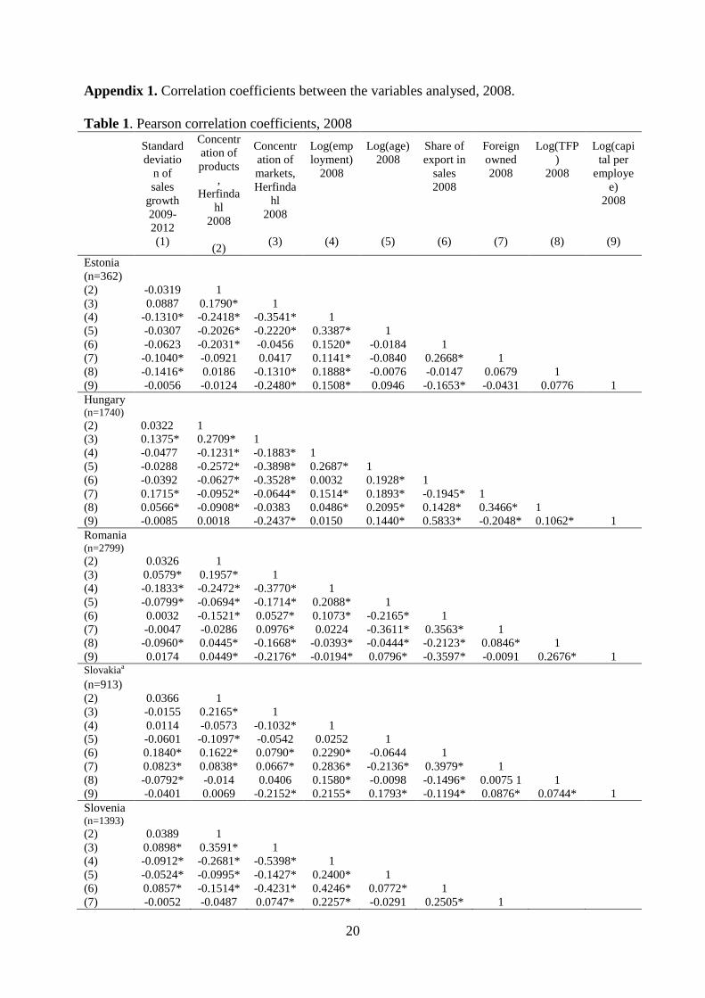
Appendix 1 presents the correlation coefficients of the variables analysed. These descriptive

correlations support our specification. Size, age and export share are usually strongly

correlated with export diversification and less strongly correlated with volatility. The total

factor productivity is usually strongly negatively correlated with volatility and less strongly

related to the diversification of trade. It is also notable that the correlation between the

diversification of products and the diversification of destination markets is relatively weak.

9

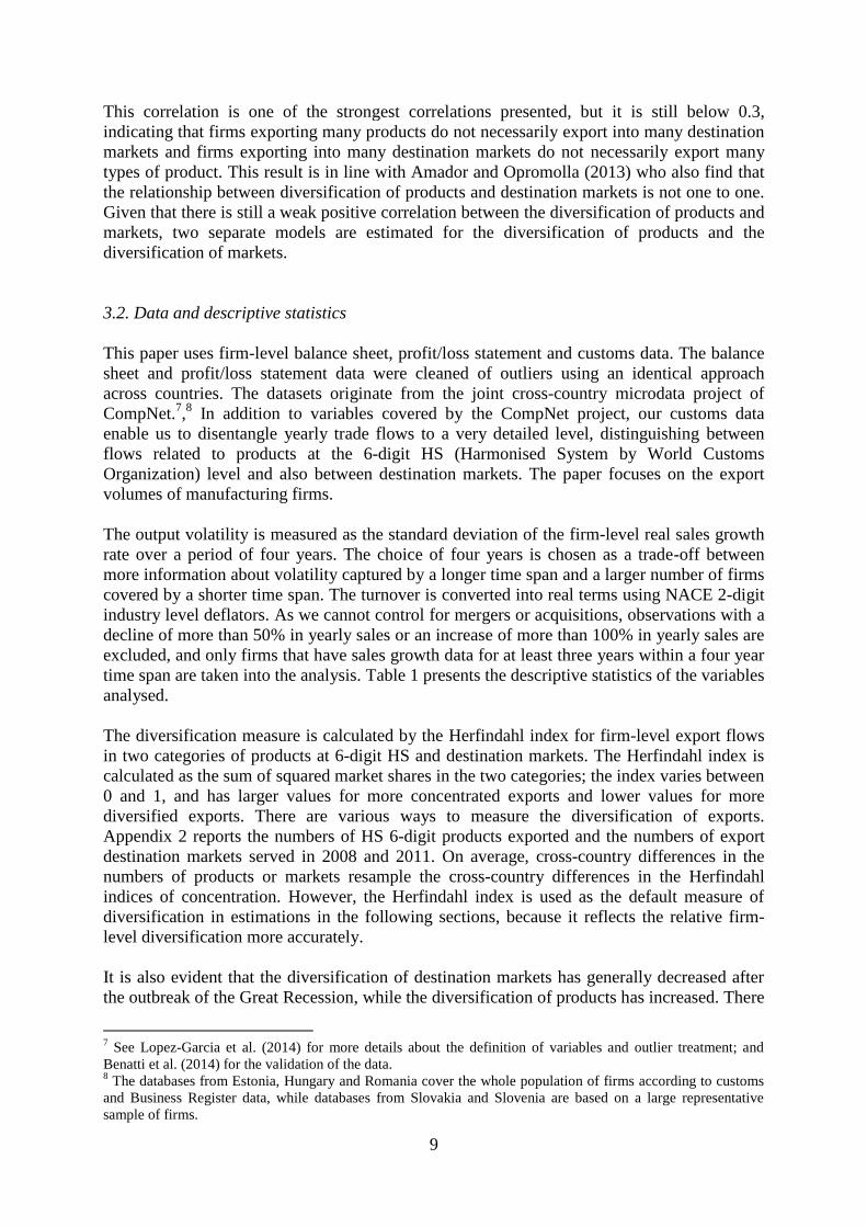
This correlation is one of the strongest correlations presented, but it is still below 0.3,

indicating that firms exporting many products do not necessarily export into many destination

markets and firms exporting into many destination markets do not necessarily export many

types of product. This result is in line with Amador and Opromolla (2013) who also find that

the relationship between diversification of products and destination markets is not one to one.

Given that there is still a weak positive correlation between the diversification of products and

markets, two separate models are estimated for the diversification of products and the

diversification of markets.

3.2. Data and descriptive statistics

This paper uses firm-level balance sheet, profit/loss statement and customs data. The balance

sheet and profit/loss statement data were cleaned of outliers using an identical approach

across countries. The datasets originate from the joint cross-country microdata project of

CompNet.7,8 In addition to variables covered by the CompNet project, our customs data

enable us to disentangle yearly trade flows to a very detailed level, distinguishing between

flows related to products at the 6-digit HS (Harmonised System by World Customs

Organization) level and also between destination markets. The paper focuses on the export

volumes of manufacturing firms.

The output volatility is measured as the standard deviation of the firm-level real sales growth

rate over a period of four years. The choice of four years is chosen as a trade-off between

more information about volatility captured by a longer time span and a larger number of firms

covered by a shorter time span. The turnover is converted into real terms using NACE 2-digit

industry level deflators. As we cannot control for mergers or acquisitions, observations with a

decline of more than 50% in yearly sales or an increase of more than 100% in yearly sales are

excluded, and only firms that have sales growth data for at least three years within a four year

time span are taken into the analysis. Table 1 presents the descriptive statistics of the variables

analysed.

The diversification measure is calculated by the Herfindahl index for firm-level export flows

in two categories of products at 6-digit HS and destination markets. The Herfindahl index is

calculated as the sum of squared market shares in the two categories; the index varies between

0 and 1, and has larger values for more concentrated exports and lower values for more

diversified exports. There are various ways to measure the diversification of exports.

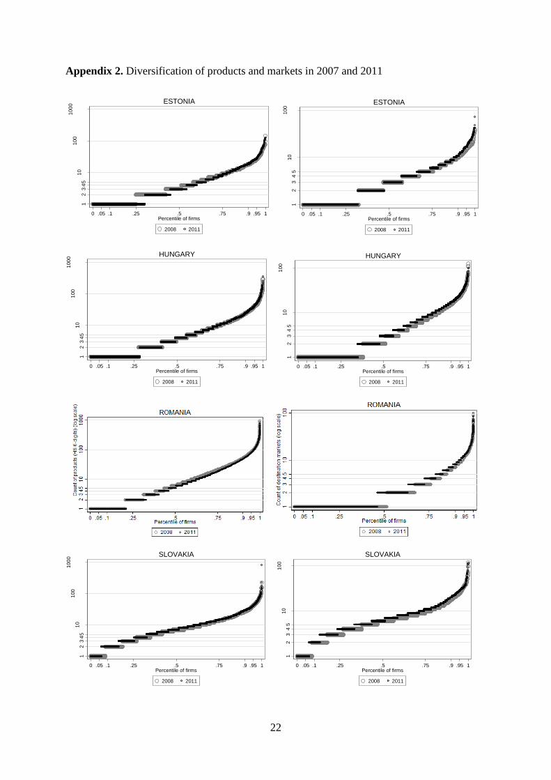
Appendix 2 reports the numbers of HS 6-digit products exported and the numbers of export

destination markets served in 2008 and 2011. On average, cross-country differences in the

numbers of products or markets resample the cross-country differences in the Herfindahl

indices of concentration. However, the Herfindahl index is used as the default measure of

diversification in estimations in the following sections, because it reflects the relative firm-

level diversification more accurately.

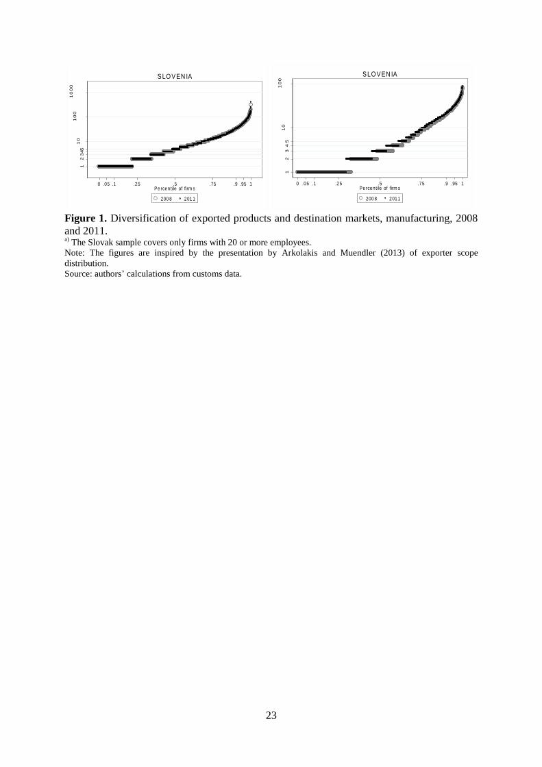
It is also evident that the diversification of destination markets has generally decreased after

the outbreak of the Great Recession, while the diversification of products has increased. There

7 See Lopez-Garcia et al. (2014) for more details about the definition of variables and outlier treatment; and

Benatti et al. (2014) for the validation of the data. 8 The databases from Estonia, Hungary and Romania cover the whole population of firms according to customs

and Business Register data, while databases from Slovakia and Slovenia are based on a large representative

sample of firms.

10

are noticeable differences across the sample countries, as Estonian, Hungarian and Slovenian

firms are diversified relatively little, with around one quarter to one third of firms exporting

just one product or to one country, while Slovak firms are much more diversified, as only

10% of firms export one product or to one destination. The higher diversification in Slovakia

is probably related to the characteristics of the sample, as only firms with 20 or more

employees are covered. Exports by Romanian firms are more concentrated in destination

markets, with up to half of firms exporting to only one country. Romania also has the highest

concentration in the sample of destination markets at the aggregate level, see Section 2.2.

The sample firms are more volatile and more concentrated in terms of exports than the data in

previous studies show (Buch et al. (2009) and Vannoorenberghe et al. (2014)). The main

advantage of our database is that unlike previous studies we also cover small firms and use

data that cover the whole population of firms or a large representative sample of the whole

population of firms. The firms in our sample are relatively small9 and young. At the same

time they have high international openness, as the export share in the sales of firms is up to

50% on average and the share of foreign owned firms is as high as 50% on average in some of

the sample countries (Table 1).

Table 1. Descriptive statistics of the variables analysed; volatility of real sales growth rate

covers the period 2009-2012 and other variables cover 2008 Estonia

(n=362)

Hungary

(n=1740)

Romania

(n=2799)

Slovakiaa

(n=913)

Slovenia

(n=1393)

Standard deviation of sales growth: mean 0.259 0.237 0.230 0.251 0.218

standard deviation 0.131 0.130 0.129 0.159 0.120

Herfindahl index of HS6 products: mean 0.702 0.692 0.688 0.596 0.673


Herfindahl index of markets: mean 0.703 0.649 0.781 0.520 0.663


Employment: mean 54.4 4.498* 193.0 229.0 66.9

standard deviation 76.6 1.0627* 457.3 591.6 167.3

Age: mean 11.4 1.382* 12.9 11.4 2.571*

standard deviation 4.6 0.471* 5.2 5.1 0.547*

Export share in sales: mean 0.545 0.476 0.574 0.519 0.330


Share of foreign owned firms (base: domestic):

mean 0.296 0.444 0.499 0.451 0.067


Log(TFP): mean 1.436 1.154 -0.019 1.359

standard deviation 0.656 0.707 1.446 0.540

Log(capital per employee): mean 1.187 1.7349 0.940 1.944 2.528

standard deviation 1.202 1.237 1.338 0.988 1.090 a)

The Slovak sample covers only firms with 20 or more employees.

Notes: Foreign owned firms are defined as a binary variable where majority foreign owned firms take the value

"1" and the rest "0". All the monetary variables are in thousands of euros and in prices of 2005. * Denotes

variables in logarithms.

Source: authors’ calculations from customs data.

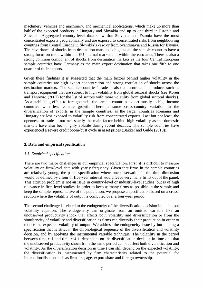
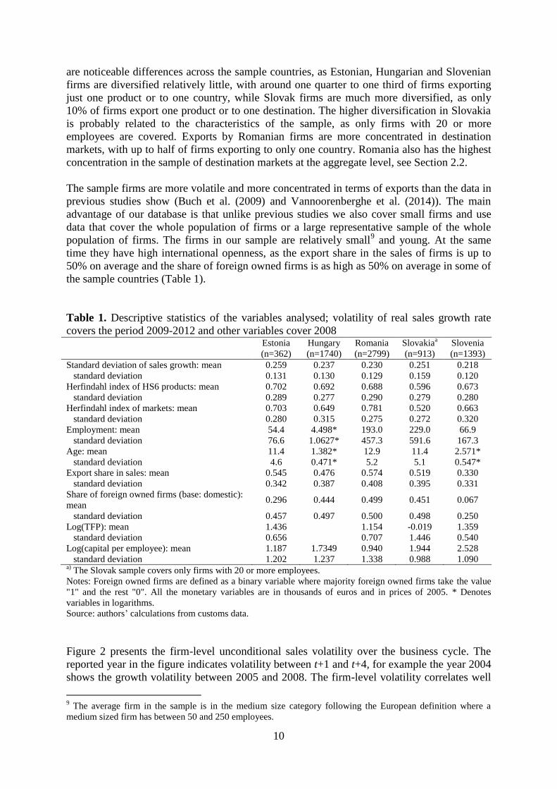
Figure 2 presents the firm-level unconditional sales volatility over the business cycle. The

reported year in the figure indicates volatility between t+1 and t+4, for example the year 2004

shows the growth volatility between 2005 and 2008. The firm-level volatility correlates well

9 The average firm in the sample is in the medium size category following the European definition where a

medium sized firm has between 50 and 250 employees.

11

with the business cycle; the volatility was low during the years of fast growth between 2005

and 2008 and increased substantially during the Great Recession in 2009. These dynamics are

captured by low volatility in 2004 and by increased volatility since 2005 in the figure. The

unconditional volatility of exporting firms is more strongly correlated with the business cycle

than the volatility of non-exporters is. The volatility of domestic firms is more stable over

time and has different dynamics in different countries. For example, Estonian and Hungarian

domestic firms faced increased volatility during the recession because of the large drop in

domestic demand, while Slovakian domestic firms have had lower volatility during the

recession as the drop in domestic demand was modest for them (see Bakker and Gulde (2010)

for an overview of the dynamics of domestic demand in CEE countries).

.16

.18

.2.2

2.2

4.2

6

Me

dia

n s

tan

da

rd d

evia

tion

of firm

sa

les g

row

th

2004 2005 2006 2007 2008

No export

Below median diversified export

Above median diversified export

ESTONIA

.16

.18

.2.2

2.2

4.2

6

Me

dia

n s

tan

da

rd d

evia

tion

of firm

sa

les g

row

th

2004 2005 2006 2007 2008

No export



ESTONIA

.16

.18

.2.2

2.2

4.2

6

Me

dia

n s

tan

da

rd d

evia

tion

of firm

sa

les g

row

th

2004 2005 2006 2007 2008

No export



HUNGARY

.16

.18

.2.2

2.2

4.2

6

Me

dia

n s

tan

da

rd d

evia

tion

of firm

sa

les g

row

th

2004 2005 2006 2007 2008

No export



HUNGARY

.16

.18

.2.2

2.2

4.2

6

Me

dia

n s

tan

da

rd d

evia

tion

of firm

sa

les g

row

th

2004 2005 2006 2007 2008

No export



ROMANIA

.16

.18

.2.2

2.2

4.2

6

Me

dia

n s

tan

da

rd d

evia

tion

of firm

sa

les g

row

th

2004 2005 2006 2007 2008

No export



ROMANIA

12

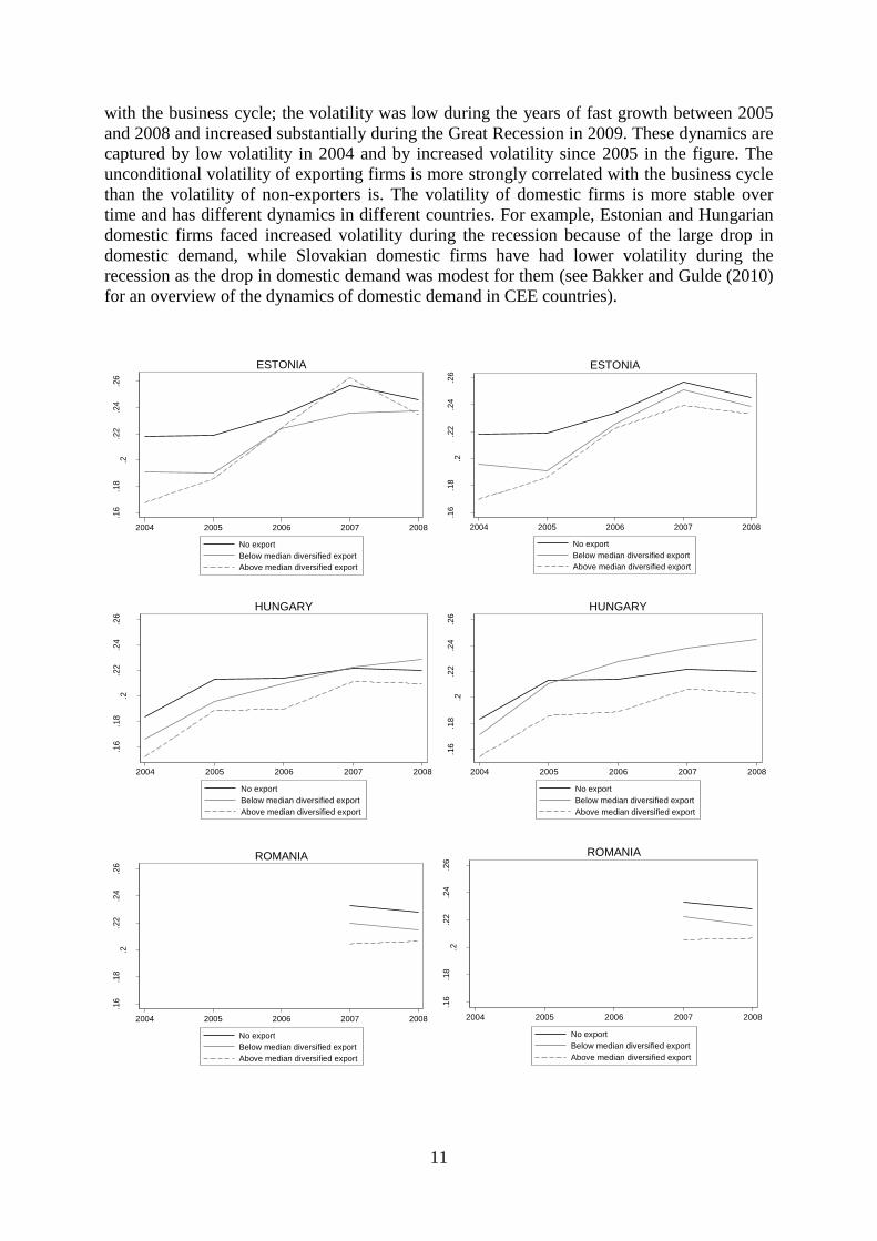
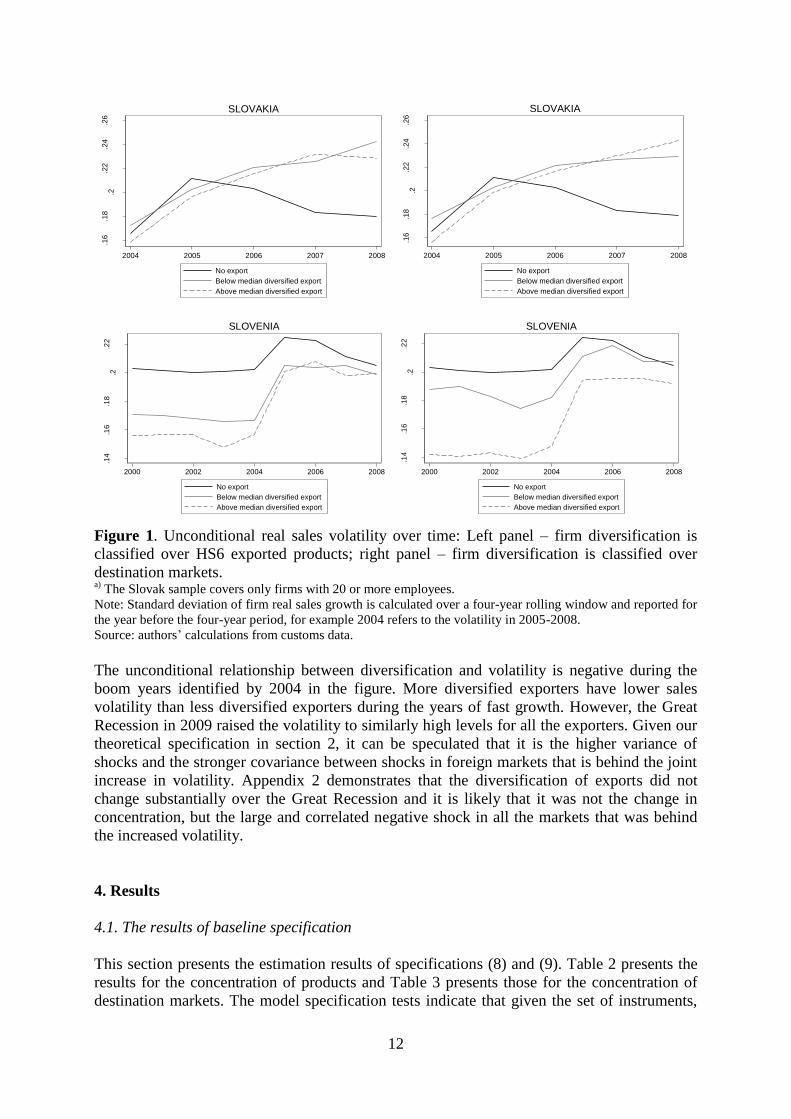
Figure 1. Unconditional real sales volatility over time: Left panel – firm diversification is

classified over HS6 exported products; right panel – firm diversification is classified over

destination markets. a)


Note: Standard deviation of firm real sales growth is calculated over a four-year rolling window and reported for

the year before the four-year period, for example 2004 refers to the volatility in 2005-2008.


The unconditional relationship between diversification and volatility is negative during the

boom years identified by 2004 in the figure. More diversified exporters have lower sales

volatility than less diversified exporters during the years of fast growth. However, the Great

Recession in 2009 raised the volatility to similarly high levels for all the exporters. Given our

theoretical specification in section 2, it can be speculated that it is the higher variance of

shocks and the stronger covariance between shocks in foreign markets that is behind the joint

increase in volatility. Appendix 2 demonstrates that the diversification of exports did not

change substantially over the Great Recession and it is likely that it was not the change in

concentration, but the large and correlated negative shock in all the markets that was behind

the increased volatility.

4. Results

4.1. The results of baseline specification

This section presents the estimation results of specifications (8) and (9). Table 2 presents the

results for the concentration of products and Table 3 presents those for the concentration of

destination markets. The model specification tests indicate that given the set of instruments,

.16

.18

.2.2

2.2

4.2

6

Me

dia

n s

tan

da

rd d

evia

tion

of firm

sa

les g

row

th

2004 2005 2006 2007 2008

No export



SLOVAKIA

.16

.18

.2.2

2.2

4.2

6

Me

dia

n s

tan

da

rd d

evia

tion

of firm

sa

les g

row

th

2004 2005 2006 2007 2008

No export



SLOVAKIA.1

4.1

6.1

8.2

.22

Med

ian s

tand

ard

devia

tion

of firm

sa

les g

row

th

2000 2002 2004 2006 2008

No export



SLOVENIA

.14

.16

.18

.2.2

2

Med

ian s

tand

ard

devia

tion

of firm

sa

les g

row

th

2000 2002 2004 2006 2008

No export



SLOVENIA

13

the exogeneity of diversification is rejected for most of the regressions. This test relies heavily

on the validity of the instruments, but the tests of overidentifying restrictions are less

encouraging and the validity of the instruments is rejected for Hungary, Romania and

Slovenia. The results of the specification tests differ across timespans and countries (see

Appendix 3), for example estimations from around 2005 show the validity of instruments for

all the sample countries. Given that the coefficients are also rather similar for all the countries,

we maintain an identical specification across countries.

The instruments applied are usually strongly correlated with the concentration in the first

stage, indicating that the weak instrument problem is not substantial. The first-stage equation

for concentration shows that larger and older firms and firms with higher export intensity

have more diversified exports of products, while the total factor productivity and capital

intensity that enter the volatility equation usually have a weaker correlation with

diversification. Foreign-owned firms have more concentrated exports than domestic firms in

terms of destination markets, but not in terms of products exported. It can be speculated that

foreign-owned firms are integrated with business groups by specialisation in destination

markets and not by specialisation in products.

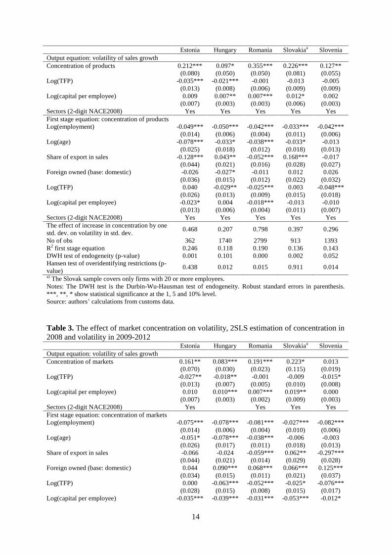
The output equation demonstrates that the concentrations of products and destination markets

have a strong positive effect on volatility. The size of the effect is large, as higher

concentration of one standard deviation is related to higher volatility of 0.2 to 0.8 of a

standard deviation. Romanian firms benefit more from higher diversification, while the

Hungarian firms benefit less. Coefficients for the remaining explanatory variables also have

the expected signs in the output equation; more productive firms have lower volatility and

more capital intensive firms have higher volatility. In line with the theory, more productive

firms enjoy a larger scope for internal adjustments. The positive relationship between capital

intensity and volatility can be related to lower adjustment costs for capital than for labour.

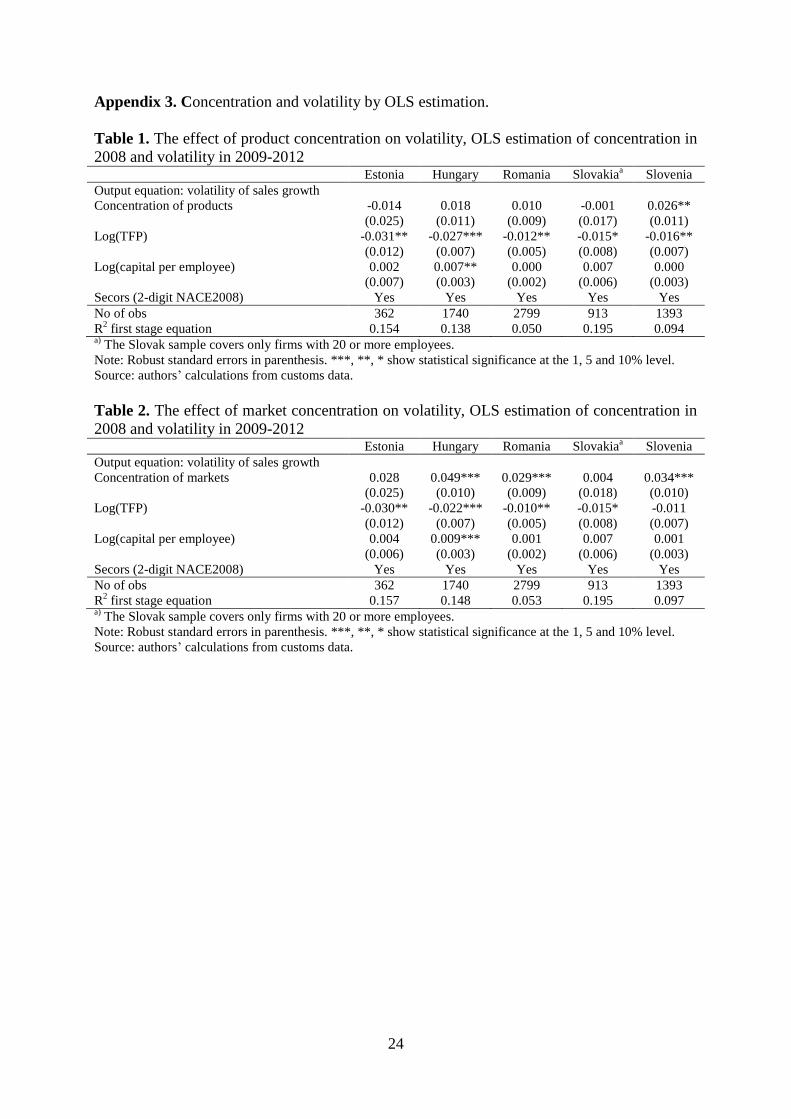
As expected, the 2SLS coefficient for concentration is much larger than the coefficient from

OLS. We proposed in the section on the empirical specification that an inability to control for

the potential for internationalisation in OLS biases the effect of concentration on volatility

downwards (see Appendix 3 for OLS results).

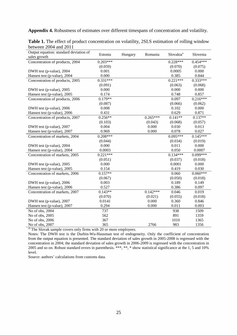
It is also evident that the diversification of products has a stronger effect on volatility than the

diversification of destination markets. Appendix 4 demonstrates that this regularity holds

throughout the business cycle and is not related to the time period over the Great Recession

presented in Tables 2 and 3. However, the effect of diversification on volatility decreased

during the recession in all the sample countries (see Appendix 4). This finding is in line with

our theoretical specification in Section 2.1. The covariance of shocks in all the markets

increased due to the joint global shock in all the markets, and the contribution of the

diversification component to volatility weakened. In other words, both the unconditional and

conditional effects of diversification on volatility decreased during the recession.

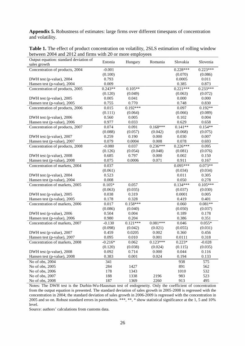
Appendix 5 tests whether the diversification effect is different for larger firms. The negative

relationship between diversification and volatility also holds for larger firms, but is smaller in

size and less frequently statistically significant.

Table 2. The effect of product concentration on volatility, 2SLS estimation of concentration

in 2008 and volatility in 2009-2012

14

Estonia Hungary Romania Slovakiaa Slovenia

Output equation: volatility of sales growth

Concentration of products 0.212*** 0.097* 0.355*** 0.226*** 0.127**

(0.080) (0.050) (0.050) (0.081) (0.055)

Log(TFP) -0.035*** -0.021*** -0.001 -0.013 -0.005

(0.013) (0.008) (0.006) (0.009) (0.009)

Log(capital per employee) 0.009 0.007** 0.007*** 0.012* 0.002

(0.007) (0.003) (0.003) (0.006) (0.003)

Sectors (2-digit NACE2008) Yes Yes Yes Yes Yes

First stage equation: concentration of products

Log(employment) -0.049*** -0.050*** -0.042*** -0.033*** -0.042***

(0.014) (0.006) (0.004) (0.011) (0.006)

Log(age) -0.078*** -0.033* -0.038*** -0.033* -0.013

(0.025) (0.018) (0.012) (0.018) (0.013)

Share of export in sales -0.128*** 0.043** -0.052*** 0.168*** -0.017

(0.044) (0.021) (0.016) (0.028) (0.027)

Foreign owned (base: domestic) -0.026 -0.027* -0.011 0.012 0.026

(0.036) (0.015) (0.012) (0.022) (0.032)

Log(TFP) 0.040 -0.029** -0.025*** 0.003 -0.048***

(0.026) (0.013) (0.009) (0.015) (0.018)

Log(capital per employee) -0.023* 0.004 -0.018*** -0.013 -0.010

(0.013) (0.006) (0.004) (0.011) (0.007)


The effect of increase in concentration by one

std. dev. on volatility in std. dev. 0.468 0.207 0.798 0.397 0.296

No of obs 362 1740 2799 913 1393

R2 first stage equation 0.246 0.118 0.190 0.136 0.143

DWH test of endogeneity (p-value) 0.001 0.101 0.000 0.002 0.052

Hansen test of overidentifying restrictions (p-

value) 0.438 0.012 0.015 0.911 0.014

a) The Slovak sample covers only firms with 20 or more employees.

Notes: The DWH test is the Durbin-Wu-Hausman test of endogeneity. Robust standard errors in parenthesis.

***, **, * show statistical significance at the 1, 5 and 10% level.


Table 3. The effect of market concentration on volatility, 2SLS estimation of concentration in

2008 and volatility in 2009-2012 Estonia Hungary Romania Slovakia

a Slovenia


Concentration of markets 0.161** 0.083*** 0.191*** 0.223* 0.013

(0.070) (0.030) (0.023) (0.115) (0.019)

Log(TFP) -0.027** -0.018** -0.001 -0.009 -0.015*

(0.013) (0.007) (0.005) (0.010) (0.008)

Log(capital per employee) 0.010 0.010*** 0.007*** 0.019** 0.000

(0.007) (0.003) (0.002) (0.009) (0.003)

Sectors (2-digit NACE2008) Yes Yes Yes Yes

First stage equation: concentration of markets

Log(employment) -0.075*** -0.078*** -0.081*** -0.027*** -0.082***

(0.014) (0.006) (0.004) (0.010) (0.006)

Log(age) -0.051* -0.078*** -0.038*** -0.006 -0.003

(0.026) (0.017) (0.011) (0.018) (0.013)

Share of export in sales -0.066 -0.024 -0.059*** 0.062** -0.297***

(0.044) (0.021) (0.014) (0.029) (0.028)

Foreign owned (base: domestic) 0.044 0.090*** 0.068*** 0.066*** 0.125***

(0.034) (0.015) (0.011) (0.021) (0.037)

Log(TFP) 0.000 -0.063*** -0.052*** -0.025* -0.076***

(0.028) (0.015) (0.008) (0.015) (0.017)

Log(capital per employee) -0.035*** -0.039*** -0.031*** -0.053*** -0.012*

15

(0.013) (0.006) (0.004) (0.010) (0.006)


The effect of increase in concentration by one

std. dev. on volatility in std. dev. 0.355 0.201 0.407 0.391 0.035

No of obs 362 1740 2799 913 1393



Hansen test of overidentifying restrictions (p-

value) 0.092 0.063 0.001 0.194 0.001


Notes: The DWH test is the Durbin-Wu-Hausman test of endogeneity. Robust standard errors in parenthesis.

***, **, * show statistical significance at the 1, 5 and 10% level.


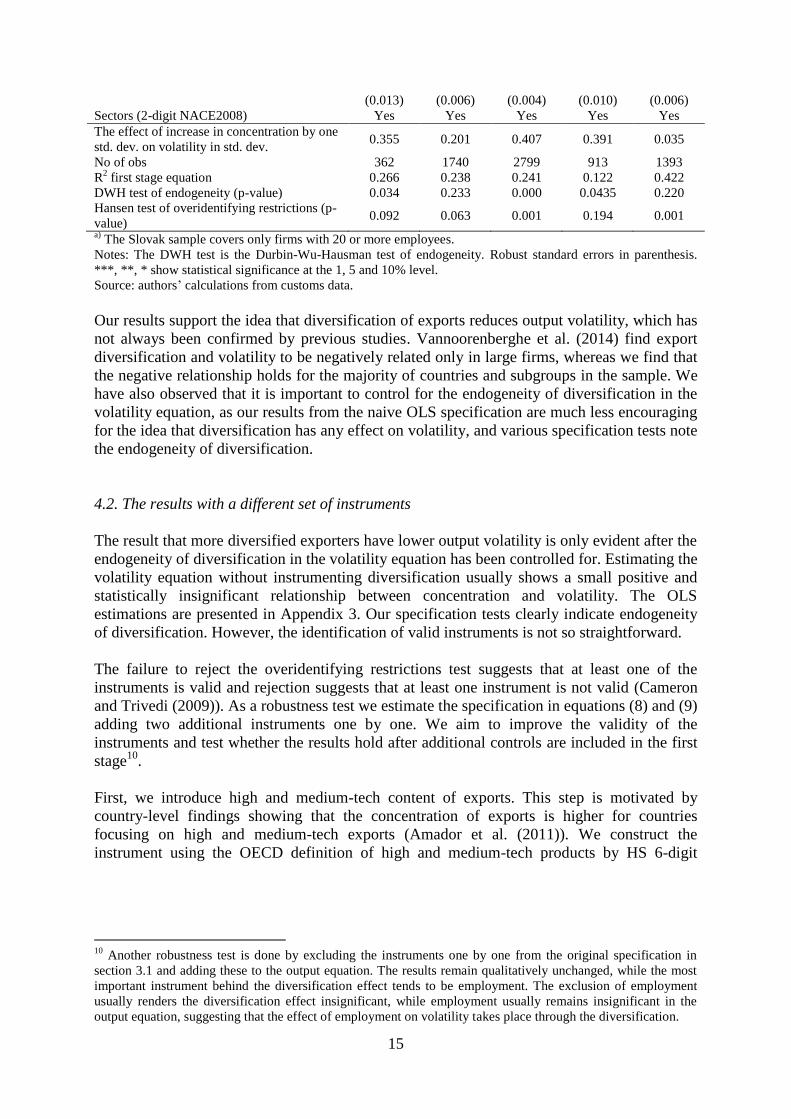
Our results support the idea that diversification of exports reduces output volatility, which has

not always been confirmed by previous studies. Vannoorenberghe et al. (2014) find export

diversification and volatility to be negatively related only in large firms, whereas we find that

the negative relationship holds for the majority of countries and subgroups in the sample. We

have also observed that it is important to control for the endogeneity of diversification in the

volatility equation, as our results from the naive OLS specification are much less encouraging

for the idea that diversification has any effect on volatility, and various specification tests note

the endogeneity of diversification.

4.2. The results with a different set of instruments

The result that more diversified exporters have lower output volatility is only evident after the

endogeneity of diversification in the volatility equation has been controlled for. Estimating the

volatility equation without instrumenting diversification usually shows a small positive and

statistically insignificant relationship between concentration and volatility. The OLS

estimations are presented in Appendix 3. Our specification tests clearly indicate endogeneity

of diversification. However, the identification of valid instruments is not so straightforward.

The failure to reject the overidentifying restrictions test suggests that at least one of the

instruments is valid and rejection suggests that at least one instrument is not valid (Cameron

and Trivedi (2009)). As a robustness test we estimate the specification in equations (8) and (9)

adding two additional instruments one by one. We aim to improve the validity of the

instruments and test whether the results hold after additional controls are included in the first

stage10

.

First, we introduce high and medium-tech content of exports. This step is motivated by

country-level findings showing that the concentration of exports is higher for countries

focusing on high and medium-tech exports (Amador et al. (2011)). We construct the

instrument using the OECD definition of high and medium-tech products by HS 6-digit

10

Another robustness test is done by excluding the instruments one by one from the original specification in

section 3.1 and adding these to the output equation. The results remain qualitatively unchanged, while the most

important instrument behind the diversification effect tends to be employment. The exclusion of employment

usually renders the diversification effect insignificant, while employment usually remains insignificant in the

output equation, suggesting that the effect of employment on volatility takes place through the diversification.

16

classification.11

We calculate the instrument at the firm level as the share of high and

medium-tech products in total exports.

Second, we introduce an instrument capturing potential for diversification. The instrument is

calculated by multiplying the firm’s share of exports in the total exports of the sample country

to a particular destination market by the difference between total imports to that destination

market and the imports from the sample country. The results of this multiplication are

summed for all the destination markets where the firm is exporting. The export structure is

taken from 2006, while the import structure comes from 200812

. The idea of the instrument is

to capture firms that are capable of exporting a larger share to large markets, because in these

cases exports are expected to be less concentrated as large markets are served by many firms

(Arkolakis and Muendler (2013)), and having a larger share in these markets shows the firm’s

potential ability to exceed entry costs to other markets or with other products.

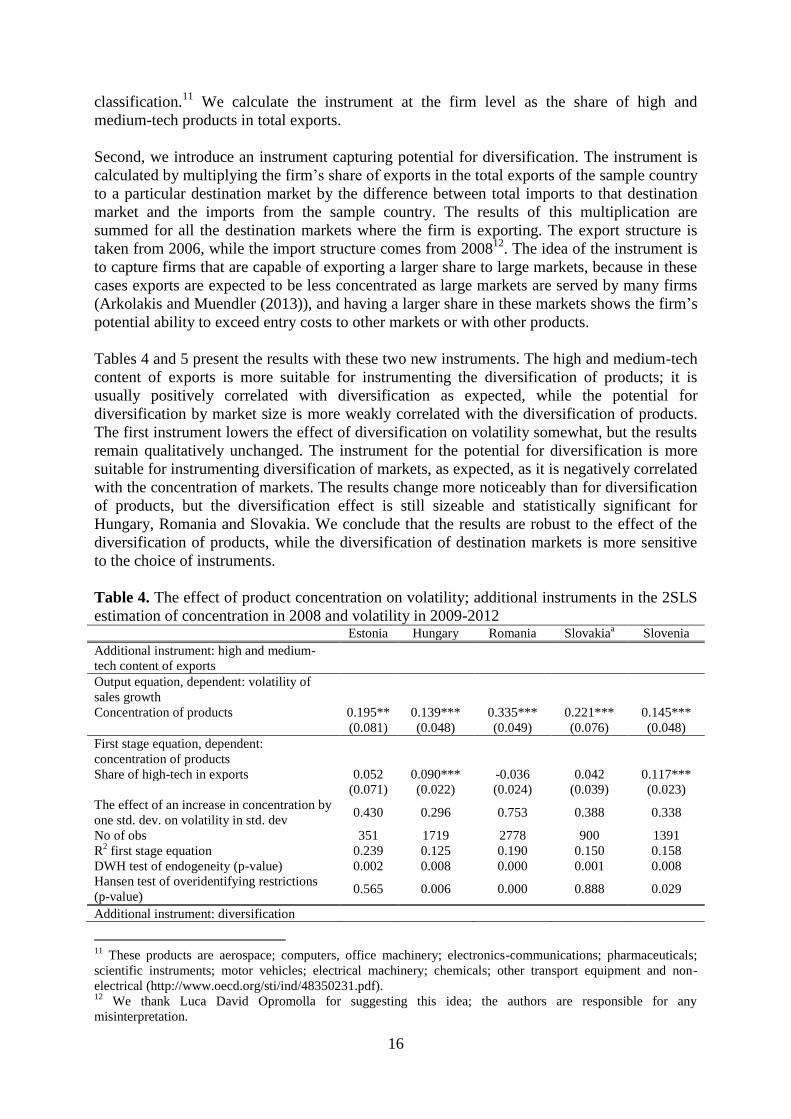
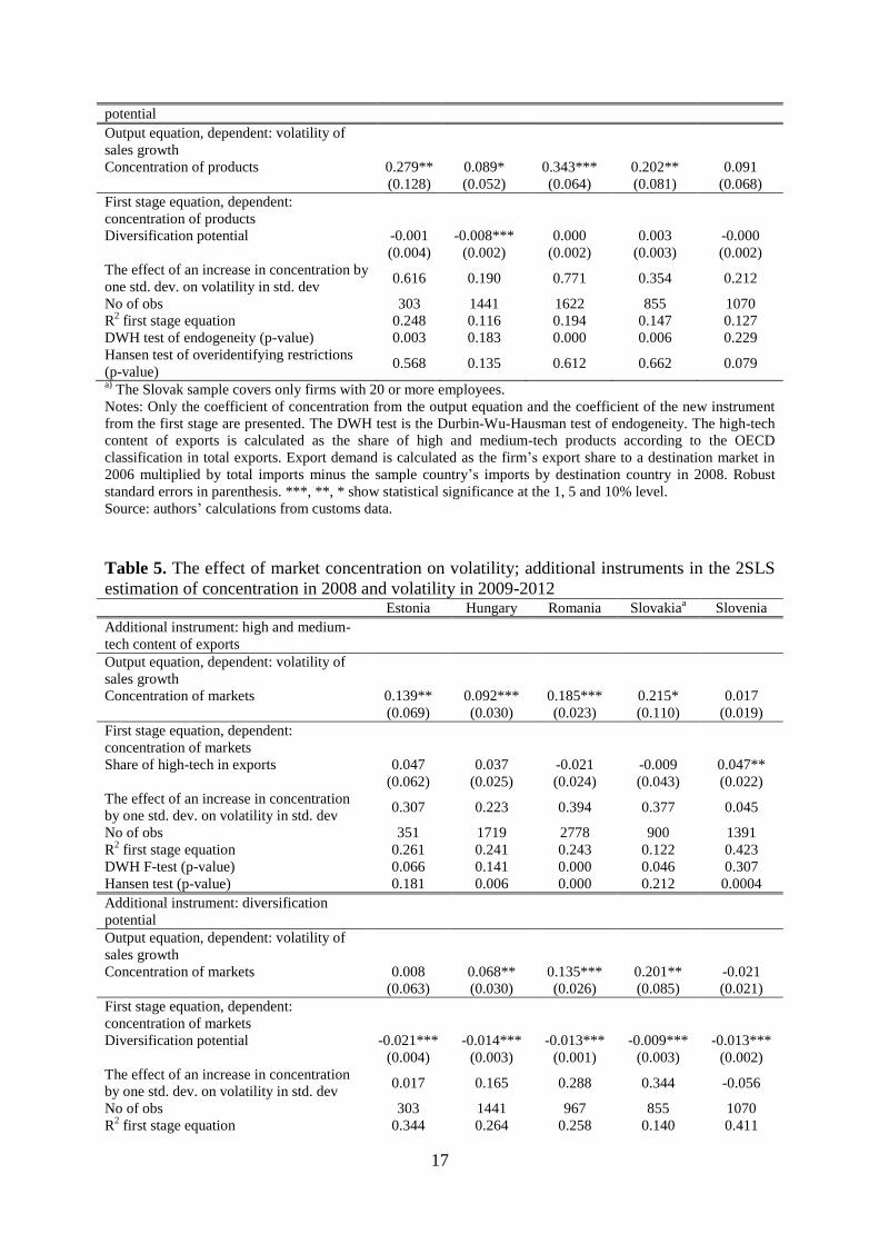
Tables 4 and 5 present the results with these two new instruments. The high and medium-tech

content of exports is more suitable for instrumenting the diversification of products; it is

usually positively correlated with diversification as expected, while the potential for

diversification by market size is more weakly correlated with the diversification of products.

The first instrument lowers the effect of diversification on volatility somewhat, but the results

remain qualitatively unchanged. The instrument for the potential for diversification is more

suitable for instrumenting diversification of markets, as expected, as it is negatively correlated

with the concentration of markets. The results change more noticeably than for diversification

of products, but the diversification effect is still sizeable and statistically significant for

Hungary, Romania and Slovakia. We conclude that the results are robust to the effect of the

diversification of products, while the diversification of destination markets is more sensitive

to the choice of instruments.

Table 4. The effect of product concentration on volatility; additional instruments in the 2SLS

estimation of concentration in 2008 and volatility in 2009-2012 Estonia Hungary Romania Slovakia

a Slovenia

Additional instrument: high and medium-

tech content of exports

Output equation, dependent: volatility of

sales growth

Concentration of products 0.195** 0.139*** 0.335*** 0.221*** 0.145***

(0.081) (0.048) (0.049) (0.076) (0.048)

First stage equation, dependent:

concentration of products

Share of high-tech in exports 0.052 0.090*** -0.036 0.042 0.117***

(0.071) (0.022) (0.024) (0.039) (0.023)

The effect of an increase in concentration by

one std. dev. on volatility in std. dev 0.430 0.296 0.753 0.388 0.338

No of obs 351 1719 2778 900 1391



Hansen test of overidentifying restrictions

(p-value) 0.565 0.006 0.000 0.888 0.029

Additional instrument: diversification

11

These products are aerospace; computers, office machinery; electronics-communications; pharmaceuticals;

scientific instruments; motor vehicles; electrical machinery; chemicals; other transport equipment and non-

electrical (http://www.oecd.org/sti/ind/48350231.pdf). 12

We thank Luca David Opromolla for suggesting this idea; the authors are responsible for any

misinterpretation.

17

potential


sales growth

Concentration of products 0.279** 0.089* 0.343*** 0.202** 0.091

(0.128) (0.052) (0.064) (0.081) (0.068)


concentration of products

Diversification potential -0.001 -0.008*** 0.000 0.003 -0.000

(0.004) (0.002) (0.002) (0.003) (0.002)

The effect of an increase in concentration by

one std. dev. on volatility in std. dev 0.616 0.190 0.771 0.354 0.212

No of obs 303 1441 1622 855 1070



Hansen test of overidentifying restrictions

(p-value) 0.568 0.135 0.612 0.662 0.079


Notes: Only the coefficient of concentration from the output equation and the coefficient of the new instrument

from the first stage are presented. The DWH test is the Durbin-Wu-Hausman test of endogeneity. The high-tech

content of exports is calculated as the share of high and medium-tech products according to the OECD

classification in total exports. Export demand is calculated as the firm’s export share to a destination market in

2006 multiplied by total imports minus the sample country’s imports by destination country in 2008. Robust

standard errors in parenthesis. ***, **, * show statistical significance at the 1, 5 and 10% level.


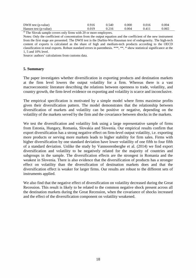
Table 5. The effect of market concentration on volatility; additional instruments in the 2SLS

estimation of concentration in 2008 and volatility in 2009-2012 Estonia Hungary Romania Slovakia

a Slovenia

Additional instrument: high and medium-

tech content of exports


sales growth

Concentration of markets 0.139** 0.092*** 0.185*** 0.215* 0.017

(0.069) (0.030) (0.023) (0.110) (0.019)


concentration of markets

Share of high-tech in exports 0.047 0.037 -0.021 -0.009 0.047**

(0.062) (0.025) (0.024) (0.043) (0.022)

The effect of an increase in concentration

by one std. dev. on volatility in std. dev 0.307 0.223 0.394 0.377 0.045

No of obs 351 1719 2778 900 1391


DWH F-test (p-value) 0.066 0.141 0.000 0.046 0.307

Hansen test (p-value) 0.181 0.006 0.000 0.212 0.0004

Additional instrument: diversification

potential


sales growth

Concentration of markets 0.008 0.068** 0.135*** 0.201** -0.021

(0.063) (0.030) (0.026) (0.085) (0.021)


concentration of markets

Diversification potential -0.021*** -0.014*** -0.013*** -0.009*** -0.013***

(0.004) (0.003) (0.001) (0.003) (0.002)

The effect of an increase in concentration

by one std. dev. on volatility in std. dev 0.017 0.165 0.288 0.344 -0.056

No of obs 303 1441 967 855 1070


18

DWH test (p-value) 0.916 0.540 0.000 0.016 0.004

Hansen test (p-value) 0.019 0.216 0.004 0.411 0.065 a)


Notes: Only the coefficient of concentration from the output equation and the coefficient of the new instrument

from the first stage are presented. The DWH test is the Durbin-Wu-Hausman test of endogeneity. The high-tech

content of exports is calculated as the share of high and medium-tech products according to the OECD

classification in total exports. Robust standard errors in parenthesis. ***, **, * show statistical significance at the

1, 5 and 10% level.


5. Summary

The paper investigates whether diversification in exporting products and destination markets

at the firm level lowers the output volatility for a firm. Whereas there is a vast

macroeconomic literature describing the relations between openness to trade, volatility, and

country growth, the firm-level evidence on exporting and volatility is scarce and inconclusive.

The empirical specification is motivated by a simple model where firms maximise profits

given their diversification pattern. The model demonstrates that the relationship between

diversification of markets and volatility can be positive or negative, depending on the

volatility of the markets served by the firm and the covariance between shocks in the markets.

We test the diversification and volatility link using a large representative sample of firms

from Estonia, Hungary, Romania, Slovakia and Slovenia. Our empirical results confirm that

export diversification has a strong negative effect on firm-level output volatility, i.e. exporting

more products or serving more markets leads to higher stability for firm sales. Firms with

higher diversification by one standard deviation have lower volatility of one fifth to four fifth

of a standard deviation. Unlike the study by Vannoorenberghe et al. (2014) we find export

diversification and volatility to be negatively related for the majority of countries and

subgroups in the sample. The diversification effects are the strongest in Romania and the

weakest in Slovenia. There is also evidence that the diversification of products has a stronger

effect on volatility than the diversification of destination markets does and that the

diversification effect is weaker for larger firms. Our results are robust to the different sets of

instruments applied.

We also find that the negative effect of diversification on volatility decreased during the Great

Recession. This result is likely to be related to the common negative shock present across all

the destination markets during the Great Recession, when the covariance of shocks increased

and the effect of the diversification component on volatility weakened.

19

References

Arkolakis, C.; Muendler, M.-A. (2013) Exporters and Their Products: A Collection of

Empirical Regularities. CESifo Economic Studies, 59(2), 223–248.

Amador, J.; Cabral, S.; Maria, J., R. (2011) A Simple Cross-Country Index of Trade

Specialization. Open Economies Review, 22, 447-461.

Amador, J.; Opromolla, L., D. (2013) Product and destination mix in export markets. Review

of World Economics, 149, 23-53.

Bakker, B., B.; Gulde, A.-M. (2010) The Credit Boom in the EU New Member States: Bad

Luck or Bad Policies? IMF Working Paper WP/10/130.

Bejan, M. (2006) Trade Openness and Output Volatility, MPRA Paper no 2759.

Benatti, N.; Lamarche, P.; Perez-Duarte, S. (2014) Initial Quality Report of the CompNet

WS2 data. ECB Directorate General Statistics.

Buch, C., M.; Döpke, J.; Strotmann, H. (2009) Does Export Openness Increase Firm-level

Output Volatility? The World Economy, 32(4), 531-551.

Cameron, A., C.; Trivedi, P., K. (2009) Microeconometrics Using Stata, Stata Press.

Caselli, F.; Koren, M.; Lisicky, M.; Tenreyro, S. (2012) Diversification through Trade. mimeo

at: http://milanlisicky.cz/index_files/Diversification_through_Trade.pdf

Di Giovanni, J.; Levchenko A. (2009) Trade Openness and Volatility. The Review of

Economics and Statistics, 91(3), 558-585.

Di Giovanni, J.; Levchenko, A., A.; Méjean, I. (2014) Firms, Destinations, and Aggregate

Fluctuations. Econometrica, 82(4), 1303–1340.Gabaix, X. (2011) The Granular Origins of

Aggregate Fluctuations. Econometrica, 79(3), 733-772.

Haddad, M.; Lim, J., J.; Pancaro, C.; Saborowski, C. (2013) Trade openness reduces growth

volatility when countries are well diversified. Canadian Journal of Economics, 46(2), 765–

790.

Koren, M.; Tenreyro, S. (2007) Volatility and Development. The Quarterly Journal of

Economics, 122(1), 243-287.

Lopez-Carcia et al. (2014) Micro-based evidence of EU competitiveness: the CompNet

database. ECP Working Paper no. 1634.

Kose, M., A.; Prasad, E., S.; Terrones, M., E. (2006) How do trade and financial integration

affect the relationship between growth and volatility? Journal of International Economics, Vol

69, pp. 176– 202.

Kramarz, F.; Martin, J.; Méjean, I. (2014) Diversification in the Small and in the Large:

Evidence from Trade Networks, mimeo at:

https://www.economicdynamics.org/meetpapers/2014/paper_663.pdf.

[http://econ.duke.edu/events/archive/2014/04/02/labor-and-development-seminar-series-54]

Melitz, M., J (2003) The impact of trade on intra-industry reallocations and aggregate

industry productivity. Econometrica, Vol. 71(6), pp. 1695–1725.

Ramey, G.; Ramey, V., A. (1995) Cross-Country Evidence on the Link Between Volatility

and Growth. The American Economic Review, Vol. 85(5), pp. 1138-1151.

Rodrik, D. (1998) Why Do More Open Economies Have Bigger Governments? Journal of

Political Economy, 106(5), 997-1032.

Vannoorenberghe, G. (2012) Firm-level volatility and exports. Journal of International

Economics, 86, 57-67.

Vannoorenberghe, G.; . Wang, Z.; Yu, Z. (2014) Volatility and Diversification of Exports:

Firm-Level Theory and Evidence. CESifo Working Paper No. 4916, 40 p.

20

Appendix 1. Correlation coefficients between the variables analysed, 2008.

Table 1. Pearson correlation coefficients, 2008

Standard

deviatio

n of

sales

growth

2009-

2012

(1)

Concentr

ation of

products

,

Herfinda

hl

2008

(2)

Concentr

ation of

markets,

Herfinda

hl

2008

(3)

Log(emp

loyment)

2008

(4)

Log(age)

2008

(5)

Share of

export in

sales

2008

(6)

Foreign

owned

2008

(7)

Log(TFP

)

2008

(8)

Log(capi

tal per

employe

e)

2008

(9)

Estonia

(n=362)

(2) -0.0319 1

(3) 0.0887 0.1790* 1

(4) -0.1310* -0.2418* -0.3541* 1

(5) -0.0307 -0.2026* -0.2220* 0.3387* 1

(6) -0.0623 -0.2031* -0.0456 0.1520* -0.0184 1

(7) -0.1040* -0.0921 0.0417 0.1141* -0.0840 0.2668* 1

(8) -0.1416* 0.0186 -0.1310* 0.1888* -0.0076 -0.0147 0.0679 1

(9) -0.0056 -0.0124 -0.2480* 0.1508* 0.0946 -0.1653* -0.0431 0.0776 1

Hungary (n=1740)

(2) 0.0322 1

(3) 0.1375* 0.2709* 1

(4) -0.0477 -0.1231* -0.1883* 1

(5) -0.0288 -0.2572* -0.3898* 0.2687* 1

(6) -0.0392 -0.0627* -0.3528* 0.0032 0.1928* 1

(7) 0.1715* -0.0952* -0.0644* 0.1514* 0.1893* -0.1945* 1

(8) 0.0566* -0.0908* -0.0383 0.0486* 0.2095* 0.1428* 0.3466* 1

(9) -0.0085 0.0018 -0.2437* 0.0150 0.1440* 0.5833* -0.2048* 0.1062* 1

Romania (n=2799)

(2) 0.0326 1

(3) 0.0579* 0.1957* 1

(4) -0.1833* -0.2472* -0.3770* 1

(5) -0.0799* -0.0694* -0.1714* 0.2088* 1

(6) 0.0032 -0.1521* 0.0527* 0.1073* -0.2165* 1

(7) -0.0047 -0.0286 0.0976* 0.0224 -0.3611* 0.3563* 1

(8) -0.0960* 0.0445* -0.1668* -0.0393* -0.0444* -0.2123* 0.0846* 1

(9) 0.0174 0.0449* -0.2176* -0.0194* 0.0796* -0.3597* -0.0091 0.2676* 1 Slovakiaa

(n=913)

(2) 0.0366 1

(3) -0.0155 0.2165* 1

(4) 0.0114 -0.0573 -0.1032* 1

(5) -0.0601 -0.1097* -0.0542 0.0252 1

(6) 0.1840* 0.1622* 0.0790* 0.2290* -0.0644 1

(7) 0.0823* 0.0838* 0.0667* 0.2836* -0.2136* 0.3979* 1

(8) -0.0792* -0.014 0.0406 0.1580* -0.0098 -0.1496* 0.0075 1 1

(9) -0.0401 0.0069 -0.2152* 0.2155* 0.1793* -0.1194* 0.0876* 0.0744* 1

Slovenia (n=1393)

(2) 0.0389 1

(3) 0.0898* 0.3591* 1

(4) -0.0912* -0.2681* -0.5398* 1

(5) -0.0524* -0.0995* -0.1427* 0.2400* 1

(6) 0.0857* -0.1514* -0.4231* 0.4246* 0.0772* 1

(7) -0.0052 -0.0487 0.0747* 0.2257* -0.0291 0.2505* 1

21

(8) -0.1001* -0.1411* -0.2796* 0.3480* 0.0306 0.0861* 0.1494* 1

(9) -0.0204 -0.0200 -0.0696* 0.0481 0.1649* 0.0245 -0.0195 0.0734* 1 a)


Note: * denotes statistical significance at the 5% level.

22

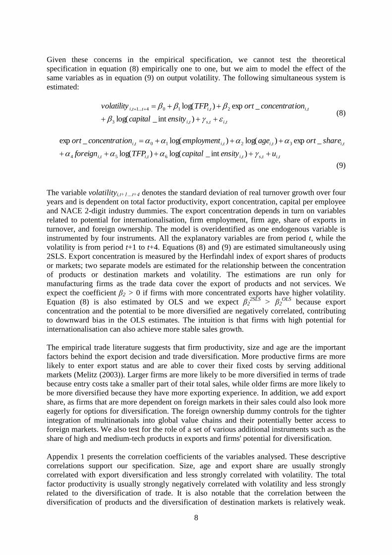
Appendix 2. Diversification of products and markets in 2007 and 2011

12

34

51

01

00

100

0

Cou

nt o

f pro

du

cts

, H

S 6

-dig

its (

log s

cale

)

0 .05 .1 .25 .5 .75 .9 .95 1Percentile of firms

2008 2011

ESTONIA

12

34

51

01

00

Cou

nt o

f de

stina

tion

ma

rkets

(lo

g s

ca

le)


2008 2011

ESTONIA

12

34

51

01

00

100

0

Cou

nt o

f pro

du

cts

, H

S 6

-dig

its (

log s

cale

)


2008 2011

HUNGARY

12

34

51

01

00

Cou

nt o

f de

stina

tion

ma

rkets

(lo

g s

ca

le)


2008 2011

HUNGARY

12

34

51

01

00

100

0

Cou

nt o

f pro

du

cts

, H

S 6

-dig

its (

log s

cale

)


2008 2011

SLOVAKIA

12

34

51

01

00

Cou

nt o

f de

stina

tion

ma

rkets

(lo

g s

ca

le)


2008 2011

SLOVAKIA

23

Figure 1. Diversification of exported products and destination markets, manufacturing, 2008

and 2011. a)


Note: The figures are inspired by the presentation by Arkolakis and Muendler (2013) of exporter scope

distribution. Source: authors’ calculations from customs data.

12

345

10

10

01

00

0

Co

un

t o

f p

rod

uc

ts (

SIT

C 5

-dig

its) (

log

sc

ale

)

0 .05 .1 .25 .5 .75 .9 .95 1Pe rcentile of firm s

200 8 201 1

SLO VEN IA

12

34

51

01

00

Co

un

t o

f d

es

tin

ati

on

ma

rke

ts (

log

sc

ale

)

0 .05 .1 .25 .5 .75 .9 .95 1Pe rcentile of firm s

200 8 201 1

SLOVEN IA

24

Appendix 3. Concentration and volatility by OLS estimation.

Table 1. The effect of product concentration on volatility, OLS estimation of concentration in


a Slovenia


Concentration of products -0.014 0.018 0.010 -0.001 0.026**

(0.025) (0.011) (0.009) (0.017) (0.011)

Log(TFP) -0.031** -0.027*** -0.012** -0.015* -0.016**

(0.012) (0.007) (0.005) (0.008) (0.007)

Log(capital per employee) 0.002 0.007** 0.000 0.007 0.000

(0.007) (0.003) (0.002) (0.006) (0.003)

Secors (2-digit NACE2008) Yes Yes Yes Yes Yes

No of obs 362 1740 2799 913 1393



Note: Robust standard errors in parenthesis. ***, **, * show statistical significance at the 1, 5 and 10% level.


Table 2. The effect of market concentration on volatility, OLS estimation of concentration in


a Slovenia


Concentration of markets 0.028 0.049*** 0.029*** 0.004 0.034***

(0.025) (0.010) (0.009) (0.018) (0.010)

Log(TFP) -0.030** -0.022*** -0.010** -0.015* -0.011

(0.012) (0.007) (0.005) (0.008) (0.007)

Log(capital per employee) 0.004 0.009*** 0.001 0.007 0.001

(0.006) (0.003) (0.002) (0.006) (0.003)

Secors (2-digit NACE2008) Yes Yes Yes Yes Yes

No of obs 362 1740 2799 913 1393



Note: Robust standard errors in parenthesis. ***, **, * show statistical significance at the 1, 5 and 10% level.


25

Appendix 4. Robustness of estimates over different timespans of concentration and volatility.

Table 1. The effect of product concentration on volatility, 2SLS estimation of rolling window

between 2004 and 2011 Output equation: standard deviation of

sales growth Estonia Hungary Romania Slovakia

a Slovenia

Concentration of products, 2004 0.203*** 0.228*** 0.454***

(0.059) (0.070) (0.075)

DWH test (p-value), 2004 0.001 0.0005 0.000

Hansen test (p-value), 2004 0.000 0.385 0.844

Concentration of products, 2005 0.331*** 0.221*** 0.333***

(0.091) (0.063) (0.068)

DWH test (p-value), 2005 0.000 0.000 0.000


Concentration of products, 2006 0.179** 0.097 0.216***

(0.087) (0.066) (0.062)

DWH test (p-value), 2006 0.008 0.102 0.000


Concentration of products, 2007 0.256** 0.265*** 0.141** 0.137**

(0.103) (0.043) (0.068) (0.057)

DWH test (p-value), 2007 0.004 0.000 0.030 0.013

Hansen test (p-value), 2007 0.969 0.000 0.078 0.027

Concentration of markets, 2004 0.208*** 0.095*** 0.145***

(0.044) (0.034) (0.019)

DWH test (p-value), 2004 0.000 0.011 0.000


Concentration of markets, 2005 0.221*** 0.134*** 0.099***

(0.051) (0.037) (0.018)

DWH test (p-value), 2005 0.000 0.0001 0.000


Concentration of markets, 2006 0.157** 0.060 0.060***

(0.067) (0.050) (0.018)

DWH test (p-value), 2006 0.003 0.189 0.149


Concentration of markets, 2007 0.143** 0.142*** 0.046 0.019

(0.070) (0.021) (0.055) (0.018)

DWH test (p-value), 2007 0.0141 0.000 0.360 0.846


No of obs, 2004 737 938 1509

No of obs, 2005 562 891 1359

No of obs, 2006 367 1010 1365

No of obs, 2007 365 2766 983 1356 a)


Notes: The DWH test is the Durbin-Wu-Hausman test of endogeneity. Only the coefficient of concentration

from the output equation is presented. The standard deviation of sales growth in 2005-2008 is regressed with the

concentration in 2004; the standard deviation of sales growth in 2006-2009 is regressed with the concentration in

2005 and so on. Robust standard errors in parenthesis. ***, **, * show statistical significance at the 1, 5 and 10%

level.


26

Appendix 5. Robustness of estimates: large firms over different timespans of concentration

and volatility.

Table 1. The effect of product concentration on volatility, 2SLS estimation of rolling window

between 2004 and 2012 and firms with 20 or more employees Output equation: standard deviation of

sales growth Estonia Hungary Romania Slovakia Slovenia

Concentration of products, 2004 -0.001 0.228*** 0.223***

(0.100) (0.070) (0.086)

DWH test (p-value), 2004 0.793 0.0005 0.011


Concentration of products, 2005 0.243** 0.105** 0.221*** 0.233***

(0.120) (0.049) (0.063) (0.072)

DWH test (p-value), 2005 0.005 0.041 0.000 0.000


Concentration of products, 2006 0.015 0.192*** 0.097 0.192**

(0.111) (0.064) (0.066) (0.089)

DWH test (p-value), 2006 0.560 0.005 0.102 0.004


Concentration of products, 2007 0.074 0.091 0.168*** 0.141** 0.154**

(0.088) (0.057) (0.042) (0.068) (0.075)

DWH test (p-value), 2007 0.259 0.190 0.000 0.030 0.007

Hansen test (p-value), 2007 0.079 0.0004 0.008 0.078 0.693

Concentration of products, 2008 -0.080 0.037 0.236*** 0.226*** 0.095

(0.126) (0.054) (0.048) (0.081) (0.076)

DWH test (p-value), 2008 0.685 0.797 0.000 0.002 0.150


Concentration of markets, 2004 0.037 0.095*** 0.073**

(0.061) (0.034) (0.034)

DWH test (p-value), 2004 0.523 0.011 0.305


Concentration of markets, 2005 0.105* 0.057 0.134*** 0.105***

(0.063) (0.035) (0.037) (0.030)

DWH test (p-value), 2005 0.038 0.319 0.0001 0.005


Concentration of markets, 2006 0.017 0.158*** 0.060 0.081**

(0.086) (0.040) (0.050) (0.037)

DWH test (p-value), 2006 0.504 0.004 0.189 0.178


Concentration of markets, 2007 -0.130 0.121*** 0.081*** 0.046 0.055*

(0.098) (0.042) (0.021) (0.055) (0.031)

DWH test (p-value), 2007 0.459 0.0205 0.002 0.360 0.456


Concentration of markets, 2008 -0.216* 0.062 0.123*** 0.223* -0.028

(0.120) (0.038) (0.024) (0.115) (0.035)

DWH test (p-value), 2008 0.092 0.714 0.000 0.044 0.116


No of obs, 2004 341 938 575

No of obs, 2005 284 1427 891 562

No of obs, 2006 178 1343 1010 532

No of obs, 2007 188 1338 2196 983 523

No of obs, 2008 187 1369 2260 913 495

Notes: The DWH test is the Durbin-Wu-Hausman test of endogeneity. Only the coefficient of concentration

from the output equation is presented. The standard deviation of sales growth in 2005-2008 is regressed with the

concentration in 2004; the standard deviation of sales growth in 2006-2009 is regressed with the concentration in

2005 and so on. Robust standard errors in parenthesis. ***, **, * show statistical significance at the 1, 5 and 10%

level.


export diversification and output volatility: comparative ... · export diversification and output...

Documents