exploring data · 2018. 11. 20. · exploring data . 6 . strata variables and nested strata strata ...

Exploring Data

This guide describes the facilities in SPM® to gain initial insights about a dataset by viewing and generating descriptive statistics.

2

© 2018 by Minitab Inc. All rights reserved.

Minitab®, SPM®, SPM Salford Predictive Modeler®, Salford Predictive Modeler®, Random Forests®, CART®, TreeNet®, MARS®, RuleLearner®, and the Minitab logo are registered trademarks of Minitab, Inc. in the United States and other countries. Additional trademarks of Minitab, Inc. can be found at www.minitab.com. All other marks referenced remain the property of their respective owners.

www.minitab.com

Salford Predictive Modeler® Exploring Data

3

Introduction to Exploring Data SPM® is a comprehensive set of tools to produce predictive, descriptive, and analytical models from datasets of any size, complexity, or organization. In many cases, though, you need to gain better understanding of the data first. The typical challenges an analyst faces when working with an unfamiliar dataset are:

• The quality of the data is not known. No matter how reputable a source of the data is it might still require data cleaning.

• Data dictionary not available or incomplete. The primary role of Variable Name is to identify a column of data. We would like it to convey the purpose and nature of the data too but this might be quite hard to achieve in many cases. Data Technologies (e.g. RDMS) are quite good at enforcing the identity of the column but are pretty indifferent to the descriptive power of the name of a variable.

These challenges usually occur at the beginning of the analysis. In SPM we made sure you have tools to get up and running with new data as soon as possible. Once a dataset is loaded you can browse raw data and obtain simple and elaborate statistics in both tabular and graphical forms.

Opening and Viewing Raw Data

Once you open a dataset, for example, using the Open button on the toolbar , data exploring features become available. In this chapter we will work with sample dataset SAMPLE.CSV supplied as part of the SPM installation. It is located in the Sample Data folder. Please refer to general SPM documentation about the ways to bring your data into SPM.

To browse raw data select View>View Data from the View menu.

You may simply click on the button in the toolbar.

As a result, the View Data window will appear.


4

This display is tailored to handle large amounts of data. The grid works in so-called “Virtual Mode”. Only current “page” of data and some cached pages are retained in memory and the dataset is queried for more pages on demand. Sometimes querying the dataset multiple times is not what you want. A good example is browsing

content from an RDBMS (SQL Server, Oracle etc). If data access latency is too large, consider extracting the data into a local file in, for example, CSV format before browsing.

Vertical scroll bar has special features to access pages of data. The buttons allow you, from top to bottom to ♦ Jump to the beginning of dataset.

♦ Jump one page up.

♦ Move one record up.

♦ Move one record down.

♦ Jump one page down.

♦ Jump to the end of the dataset.

There is a thumb-bar on the vertical scroll bar in the View Data window.

Descriptive Statistics To examine descriptive statistics of the currently open dataset, select View>Descriptive Stats… from the

View menu. You can also use the toolbar button.

As a result, the Descriptive Stats Setup window will appear.


5

The window is already configured to obtain detailed Descriptive Statistics of all of the variables in the dataset. You can press the OK button right away. The defaults are configured so that computations finish in reasonable time for small to mid-sized datasets. For this run we will use most of the features and explain the controls along the way.

Selecting Variables

The Variable Selection grid allows configuring which variables are included in the computation.

Limiting number of variables to compute by excluding ones you are not interested in can speed up computation. This is especially handy when there are variables with very high number of levels (hundreds and thousands).

To facilitate navigation through the list of variables you can sort them Alphabetically or in File Order. Search functionality is accessible through mouse right-click menu of the grid. Use the Select checkbox under the Include column to set and reset multiple checkboxes at once.

Variables can also be assigned special roles.


6

Strata variables and nested strata

STRATA <variable>

In addition to full dataset Descriptive Stats, you can request stats for sub-samples identified by levels of a specific variable. In our current dataset variable T defines Learn and Test partitions for analysis. Let’s mark T as a Strata variable.

If you have more than one variable listed on the STRATA command, you can specify whether you want nested results with the following option:

STATS <varlist> / NESTED = YES|NO

Weight variable

WEIGHT <variable>

By default each observation is accounted for only once in Descriptive Statistics computations, but you can assign any positive integer or fractional weight to each observation via a Weight variable. Let’s specify W as a weight variable.

As a result your Variable Selection should look as follows

Pre-defined Variable List Filters

There’s an alternative way to quickly select a category of variables. The Filter group of controls allows you to quickly request

• Only Character variables

• Only Numeric variables.


7

This setting overrides the selections made in the Variable Selection grid.

Configuring computation process

Computation of Descriptive Statistics can become quite resource-intensive on large and complex datasets. You can tailor the process to get the information you need in an acceptable time.

For our Sample.csv analysis, please select Detailed Stats and set both Max. distinct values to track and Max. distinct values to display to 9997.

Below each computation process configuration setting is described in more details. Note: the STATS command was formerly named DATAINFO.

Fast Stats (or Brief)

STATS <varlist> / FAST = YES

Sometimes all you need is a quick lookup of some numeric statistics (minimum, maximum, mean). Combined with the variable selection feature, you can get this information quickly.

Detailed Stats

STATS <varlist> / FAST = NO

In this mode the full set of descriptive statistics is computed. This could be quite performance-intensive even if you select just a few variables with a high number of levels and the dataset is large. There are additional controls to tailor the computation process in this mode.

Max. distinct values to track

DISCRETE MAX=<n,n>

This setting allows you to limit the number of slots to track distinct values for a variable. If a variable has more than n levels then frequency information on first n levels encountered will be available in UI. Such Frequency Tables will be labeled incomplete in the GUI.

Lowering the limit can save significant computation resources, especially when you don’t care about tabulation for continuous variables with many distinct levels.

Max. distinct values to display

STATS <varlist> / N=<n>


8

This setting limits how many levels will be displayed in the resulting frequency table. In contrast to Max. distinct values to track, this parameter has no effect on the construction of the frequency table for a specific variable. If Max. distinct values to track is greater than the number of levels large enough but Max. distinct values to display is smaller, you will get all of the stats derived from the frequency table (e.g. number of distinct values) but frequency tables themselves will be printed incomplete. But, also in contrast to Max. distinct values to track, n most frequent levels will be displayed.

Lower the limit if you do want all of the information on continuous and high-level categorical variables, but you don’t need to see full frequency tables in the results window. Showing frequencies for all distinct levels of continuous variables in a large dataset could easily exhaust UI resources.

Separate display for most and least common values

STATS <varlist> / EXTREMES = <n>

Some variables with many levels, both continuous and categorical in nature, might have a significant number of observations sharing the same value. While a full frequency table would be expensive to compute and in many cases useless, these most frequent levels might provide some useful insight. This setting allows specifying a cap on how many most and least common values to track.

Saving Descriptive Stats

Let’s save the descriptive stats for our dataset. For this, check Save to Grove checkbox and specify a file name. Your Descriptive Stats dialog should look like this:

Click OK to start the computation.

The following controls configure how results of Descriptive Stats computation are saved.

Details to Classic Output

STATS <varlist> / SILENT = NO

When this setting is ON, the Classic Output window will contain all Descriptive Stats in textual form. This might be useful if you need to compare descriptive stats for several datasets.


9

Save to Grove

GROVE "<File name>"

Just like other SPM analysis methods, Descriptive Stats can save the results into a Grove file. You can open this file in the GUI at any time to access Descriptive Stats without recomputing them.

Note: Descriptive Stats can also be saved post-computation via the Save Grove button in the resulting window.

Browsing Descriptive Stats

Once the computation is done, or if you open a Grove file containing previously computed results, you will see the Descriptive Stats window. Here’s what the results window looks like for our example:

Note the Full/Brief switch in the top right corner.

Descriptive Stats in Brief Mode

By default, the display is in Brief mode. You can quickly get an idea of ♦ How much of the data is missing?

♦ How many distinct values each column has?

♦ What are the range and the mean in each column?

♦ What are the boundaries of specific percentiles?

Note that some variables (e.g. X2, X4) have “Many Values” as the number of distinct levels. This means these variables have too many levels to tabulate given how the run was configured. The maximal number of levels for a frequency table is configured in the Descriptive Stats Setup dialog. If full tabulation is not available some of the stats are zero or empty.


10

Since we specified the Strata variable, these stats are available both for the overall dataset and for each stratum (T=0 and T=1 sheets in this particular example).

You can use the Find drop-down on the top pane to lookup a variable by name. To do this, either

♦ Select a variable from the drop-down list. Variables are always sorted in File Order.

♦ Start typing a variable name into the box. As you type, the grid will reposition itself to the variable that starts with the sub-string you typed.

The Sort drop-down allows resorting variables in the grid, either Alphabetically or in File Order. Navigation tools are quite helpful when the list of variables is large. Other controls on the bottom pane of the window allow you to

♦ Specify Precision of the numbers in the grid.

♦ Let the grid figure out the precision by checking the Auto checkbox.

♦ Align content of the cells in the grid.

♦ Choose the displayed Strata.

♦ Generate Graphs.

♦ View Commands of the SPM session.

♦ Score the descriptive statistics.

♦ Save the contents of the descriptive statistics by clicking Save Grove.

Descriptive Stats in Full Mode

Now, let’s switch to Full mode.


11

In this mode, Descriptive Stats for a variable are organized in vertical sections. Each variable occupies a column. You can use the Find and Sort drop-down menus to navigate to a specific variable. For example, type X1 into the Find box. As a result you should now see X1 in the left-most column.


12

Continue to type in X10. Now the grid scrolled to X10.

Buttons and near the title of each section allow you to expand and collapse the content. Buttons

in the top left corner of the grid are helpful to collapse or expand all the sections.

This display can also be used to get a quick idea about a particular statistic or group of statistics across all the variables. A convenient way to do this is to expand just the section of interest and scroll through all the variables.

The following sections are available.


13

Descriptive

This section contains an extended set of descriptive stats computed by the engine. There are quite a few of them in addition to ones displayed in Brief mode. This section contains the following stats: ♦ N

♦ N Missing

♦ N = 0

♦ N <> 0 (not equal to)

♦ N Distinct Values

♦ Mean

♦ Std. Deviation

♦ Skewness

♦ Coefficient Variation

♦ Conditional Mean

♦ Sum of Weights

♦ Sum

♦ Variance

♦ Kurtosis

♦ Std. Error Mean

Note that we don’t have Median and Range in the list. The reason is these values are more conveniently represented by the sections below.


14

Location

This section helps you understand the location of the variable on the number line. The relevant stats are grouped together: ♦ Mean

♦ Median

♦ Range

Variability

This section contains stats to describe the dispersion of the variable. It contains the following stats: ♦ Std. Deviation

♦ Variance

♦ Interquartile range

Quantiles

This section allows you to assess probability distribution of the variable by showing most important percentiles.

Frequency Tables


15

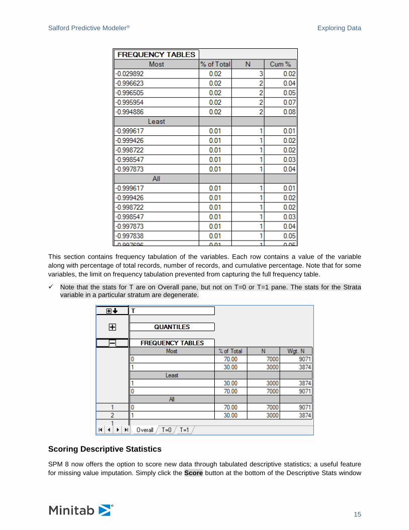
This section contains frequency tabulation of the variables. Each row contains a value of the variable along with percentage of total records, number of records, and cumulative percentage. Note that for some variables, the limit on frequency tabulation prevented from capturing the full frequency table.

Note that the stats for T are on Overall pane, but not on T=0 or T=1 pane. The stats for the Strata variable in a particular stratum are degenerate.

Scoring Descriptive Statistics

SPM 8 now offers the option to score new data through tabulated descriptive statistics; a useful feature for missing value imputation. Simply click the Score button at the bottom of the Descriptive Stats window


16

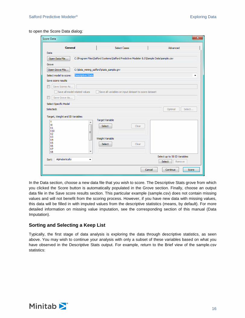
to open the Score Data dialog:

In the Data section, choose a new data file that you wish to score. The Descriptive Stats grove from which you clicked the Score button is automatically populated in the Grove section. Finally, choose an output data file in the Save score results section. This particular example (sample.csv) does not contain missing values and will not benefit from the scoring process. However, if you have new data with missing values, this data will be filled in with imputed values from the descriptive statistics (means, by default). For more detailed information on missing value imputation, see the corresponding section of this manual (Data Imputation).

Sorting and Selecting a Keep List

Typically, the first stage of data analysis is exploring the data through descriptive statistics, as seen above. You may wish to continue your analysis with only a subset of these variables based on what you have observed in the Descriptive Stats output. For example, return to the Brief view of the sample.csv statistics:


17

Sort the variable list by ascending distinct values by clicking once on the N Distinct column:

This ability to sort the variable list can be extended to all columns in this window. Now, let’s say you only wish to continue the analysis with variables that have very few distinct levels. Highlight the top 6 variables, right-click, and select New Keep List:


18

This action opens a new notepad with a KEEP statement followed by the selected variables. From here, it’s simple to submit this window to tell SPM which variables you’d like included in the analysis. You can confirm the variable selection by opening the Model Setup window.

Exploring Frequency Distributions

You can explore Frequency Distributions of variables in a graphical form. Select Explore>Frequency Distribution from the Explore menu.

As a result, the Generate Charts dialog will appear:


19

Note that the Level(s) column is not populated by default. To obtain level information, full Descriptive Stats have to be computed. This is a potentially lengthy operation. By skipping it, you can proceed directly to requesting charts for the variables of interest.

You can bring in level information by clicking the Scan Data for Levels button. This will run Descriptive Stats for all variables and populate the Level(s) column. Variable Levels Threshold control will become available to filter out variables with too many levels.


20

Since Frequency Distribution is powered by the Descriptive Stats results, you can always navigate from Descriptive Stats to a Generate Charts window via right-clicking or by clicking the Graphs button at the bottom of the window:

The controls in the Generate Charts window allow you to specify a group of charts you’re interested in seeing in a single display. You can specify Workspace Label for the group for better reference. If a variable has more than Max Bins levels, the values get binned and a histogram is displayed. Otherwise the chart will show a full frequency distribution. A variable selection grid lets you specify variables of interest.


21

Let’s request Frequency Distribution plots for all variables in the dataset. You can select the entire column and mark the Select checkbox above to select all individual variables. Once a selection is made, the Generate Charts button will be enabled.

As a result you will see a Frequency Distribution window:

Histograms are incomplete for variables with too many levels (e.g. X10 on the screenshot above). This is due to the cap on number of levels to tabulate during Descriptive Stats. Generate charts dialog uses default caps to ensure acceptable performance. You can configure your Descriptive Stats run and then request a Frequency Distribution display from it.

The Generate Charts window that you used to configure the run is still available. It keeps track of all chart groups produced and provides an easy way to navigate to each of them via the right-hand side navigation panel.


22

The Frequency Distribution window shows up to four plots at the same time. If there are more than four plots, you can scroll up and down to get to a plot of interest. The Goto Variable drop-down box is a handy way to navigate to a variable by name. You can make the Y-axis scale the same for all charts using the Same Scale button. These are just a few of the controls on the lower tool panel of the window:

Variables treated as continuous are displayed as histograms. For categorical variables, a full frequency table is displayed. By default, the decision on whether a variable is continuous or categorical comes from the SPM engine. The Treat Vars As group of controls lets you override this. In addition to the default, you can opt to treat all variables as either Continuous or Categorical. The dataset we are examining contains quite a few variables with large numbers of levels. If you request to treat them as Categorical, the Frequency Distribution will try to plot each individual level. If you navigate to X1 and click Categorical you might see something like this:


23

It is apparent that usability of these charts is limited. To improve this, you can switch the X-Axis drop-down box from All Values to Zoomed. Now you can scroll each chart horizontally and explore the levels of interest:

Let’s switch Treat Vars As back to Auto and navigate to X9. Since X9 and X10 are continuous, Binning controls determine how the levels are binned.


24

Now let’s reduce Binning number down to 5.

You can also switch between the following Bins Presets: ♦ For Custom preset, the Number of Bins slider defines the number of bins for all continuous

variables. This is the default.

♦ For Optimal preset, the number of bins is determined individually for each variable. This is useful when looking side-by-side at variables with radically different distributions.

Let’s switch back to Optimal number of bins. Note that you’re seeing essentially the same histogram for X9. Note that the left-most 6 bins are obscured by much more populated ones to the right. Let’s truncate 50% of levels using the Truncate Right control. As a result you can now see the left side of the distribution in more details.

Sometimes it is convenient to use an alternative chart type for a histogram. For each chart type, there’s a button in the Chart Type group of controls. For example, here is the same screenshot with chart type changed to Dot.


25

Exploring Correlated Variables

To compute correlations among the variables in a dataset, select Explore>Correlation from the menu or

click the shortcut in the toolbar. The Correlation Setup window will appear:

As with the Descriptive Stats setup, you have a variable selection grid with the ability to sort either alphabetically or in file order. Options to the right include: ♦ Correlation type allows for different computation measures. These include

• Sum of cross products

• Covariance

• Pearson’s product-moment


26

• Normal Euclidean distances

• Skewness

• Variance

• Spearman’s rank-order

• Kendal Tau-b rank-order

• Positive matching dichotomous

• Jaccard’s dichotomous

• Simple matching dichotomous

• Anderberg’s dichotomous

• Tanimoto’s dichotomous

• City Block distances

• All possible matrices (may be very time consuming)

♦ Speed up compute time by only using the first N records

♦ Size of printed matrices

♦ Filtering by variable type

♦ Saving correlation results to a file and/or grove

Continue with the default values by clicking OK.

Tabs with the designated correlation measure(s) will be displayed with a matrix of color-coded values. Darker red indicates a strong negative correlation, white indicates little to no correlation, and darker


27

purple indicates a strong positive correlation. Options at the bottom of the window include adjusting precision and disabling color-coding. Also reported is the largest absolution correlation present in the table and the number of records deleted. The correlation feature uses strict listwise deletion for missing data; any record with any missing variables will be omitted.

exploring data · 2018. 11. 20. · exploring data . 6 . strata variables and nested strata strata ...

Documents