exploratory methods for choosing power transformations

Exploratory Methods for Choosing Power TransformationsAuthor(s): John D. Emerson and Michael A. StotoSource: Journal of the American Statistical Association, Vol. 77, No. 377 (Mar., 1982), pp. 103-108Published by: American Statistical AssociationStable URL: http://www.jstor.org/stable/2287775 .

Accessed: 14/06/2014 10:16

Your use of the JSTOR archive indicates your acceptance of the Terms & Conditions of Use, available at .http://www.jstor.org/page/info/about/policies/terms.jsp

.JSTOR is a not-for-profit service that helps scholars, researchers, and students discover, use, and build upon a wide range ofcontent in a trusted digital archive. We use information technology and tools to increase productivity and facilitate new formsof scholarship. For more information about JSTOR, please contact [email protected].

.

American Statistical Association is collaborating with JSTOR to digitize, preserve and extend access to Journalof the American Statistical Association.

http://www.jstor.org

This content downloaded from 195.78.108.60 on Sat, 14 Jun 2014 10:16:42 AMAll use subject to JSTOR Terms and Conditions

http://www.jstor.org/action/showPublisher?publisherCode=astata

http://www.jstor.org/stable/2287775?origin=JSTOR-pdf

http://www.jstor.org/page/info/about/policies/terms.jsp


Exploratory Methods for Choosing Power

Transformations JOHN D. EMERSON and MICHAEL A. STOTO*

Power transformations can often simplify the task of de- scribing behavior in data that consist of positive meas- urements or counts. Tukey's diagnostic techniques based on two-dimensional plots are useful in searching for a suitable transformation in two types of data structures: multiple batches at different levels, and two-way tables. To these, we add plots for finding transformations in two other structures: a single batch, and y versus x. The basis for plots that indicate transformations for symmetrizing and for straightening is explored using second-order series approximations. For all four techniques, when the plot is roughly linear with slope 1 - p, the power of a transformation indicated by the plot is p. Each plot indicates whether any power transformation can be effective in achieving a desired objective.

KEY WORDS: Exploratory data analysis: Transforma- tion plots; Additivity; Symmetry; Linear regression.

1. INTRODUCTION

The objectives of data transformation include the following:

1. attaining additivity in two-way tables, 2. stabilizing spread for several parallel data sets at

different levels (as in one-way analysis of variance), 3. increasing symmetry in a single set of data, and 4. straightening a relationship between y and x (as in

linear regression).

Tukey (1977) discusses geometric techniques for finding power transformations appropriate for the first two objectives. These plots, the diagnostic plot and the spread- vs.-level plot, are summarized in Table 6. Tukey (1949), Snedecor and Cochran (1967, Sec. 11.19), and Leinhardt and Wasserman (1979) use series expansions to motivate these plots.

In this article we introduce analogous techniques whose primary objectives are symmetrizing or straight-

* John D. Emerson is Associate Professor, Department of Mathe- matics, Middlebury College, Middlebury, VT 05753. Michael A. Stoto is Assistant Professor, Kennedy School of Government, Harvard Uni- versity, Cambridge, MA 02138. This work was supported by the Na- tional Science Foundation through grant SOC75-15702. The work was done while the first author was on leave from Middlebury College. His leave at the Sidney Farber Cancer Institute and the Harvard School of Public Health was supported in part by the National Cancer Institute, DHEW, through grant CA-23415. The authors gratefully acknowledge suggestions from David Hoaglin, Frederick Mosteller, Anita Parunak, Judith Strenio, and John Tukey. The authors thank the referees and the editors for helpful comments on earlier versions of the manuscript.

ening, and we use series approximations to guide us to these techniques. Like the diagnostic plot and spread- vs.-level plot, the plots developed indicate whether a simple power transformation can achieve its objective: if the plot is nearly straight, a power transformation will be effective. Otherwise, a more complicated approach may be needed. The new plots are natural companions to the diagnostic plot and spread-vs.-level plot, because for each plot the indicated power is again given by one- minus-slope and because it results from a series approximation.

The family of power transformations considered here is defined by

( =p(y) ApyP + Bp (p * 0) (1.1)

- Aolny + Bo (p = 0). We choose the constants to satisfy two conditions:

1. 4p(M) = M, where M is the median of y, and 2. d?' (A) = 1, where the prime denotes the derivative.

This choice ensures that the transformations are monotone increasing and that they minimally change the data near the median. Thus the transformed data are "matched" to the original data set. A linear relationship exists between the transformations specified here and those stud- ied by Box and Cox (1964).

2. TRANSFORMATION PLOT FOR SYMMETRY

We define a batch as a collection of numbers or points, possibly, but not necessarily, a random sample. Let y', Y2, . ., Yn represent the data in a batch with median M. For convenience of expression, we ignore the constants in (1.1) and use yP in derivations throughout the paper; p = 0 is understood to represent a log transformation and is not explicitly included in the development.

We seek a power, p, for which the transformed batch, Y1P, Y2, . . . , YnP, is approximately symmetric. Let yq and y -q denote the lower and upper qth quantiles: thus, for 0 < q < I, (100q) percent of the batch is below yq and an equal part is above YI-qq

If the transformed batch is perfectly symmetric, then for all quantiles we have

YqP + Y-q4 = Mp. (2.1) 2

? Journal of the American Statistical Association March 1982, Volume 77, Number 377

Theory and Methods Section

103



104 Journal of the American Statistical Association, March 1982

The expressions on the left are sometimes called midsummaries. For p * 0, a second-order Taylor-series expansion of yqP and Yi qP about M gives (except for a minus sign throughout if p < 0):

yqP ~MP+pMp-1(yq -M)

Yqp -q MP + PMP - I(Yq - -M) + - _ MP-2(yq _ M)2

2

and

Yi -qp- MP + PMP '(YI -q - M)

2 (p-_1) Mp2(yi -q - M)2.

After substituting these into (2.1) and rearranging, we obtain

Yq + YI-q M 2 (2.2)

(- p) (YI-q - M)2 + (M - Yq)2 4M

Note that, because we are dealing with nonnegative meas- urements or counts, M must be positive.

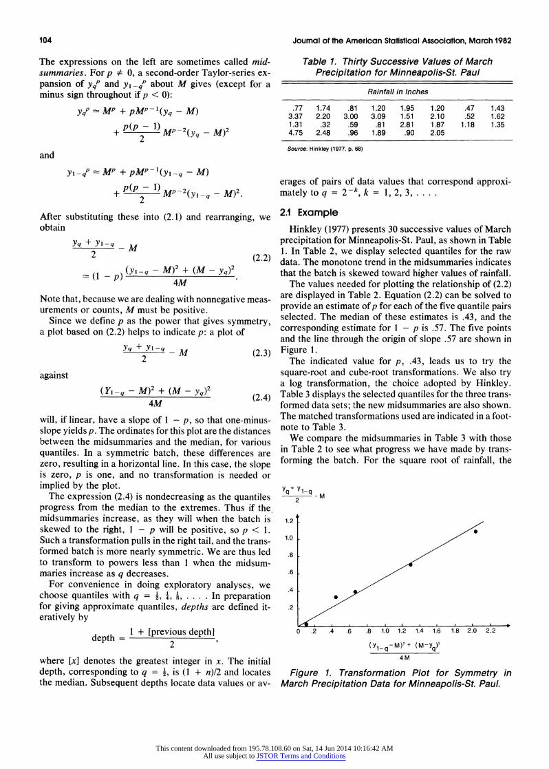
Since we define p as the power that gives symmetry, a plot based on (2.2) helps to indicate p: a plot of

Yq + YI-q _ M (2.3) 2

against

(Yl-q - M)2 + (M - Yq)2 (2.4) 4M

will, if linear, have a slope of 1 - p, so that one-minus- slope yields p. The ordinates for this plot are the distances between the midsummaries and the median, for various quantiles. In a symmetric batch, these differences are zero, resulting in a horizontal line. In this case, the slope is zero, p is one, and no transformation is needed or implied by the plot.

The expression (2.4) is nondecreasing as the quantiles progress from the median to the extremes. Thus if the midsummaries increase, as they will when the batch is skewed to the right, 1 - p will be positive, so p < 1. Such a transformation pulls in the right tail, and the transformed batch is more nearly symmetric. We are thus led to transform to powers less than 1 when the midsum- marnes increase as q decreases.

For convenience in doing exploratory analyses, we choose quantiles with q = '2,, 48, .... In preparation for giving approximate quantiles, depths are defined it- eratively by

depth = 1 + [previous depth] 2

where [x] denotes the greatest integer in x. The initial depth, corresponding to q = -, is (1 + n)l2 and locates the median. Subsequent depths locate data values or av-

Table 1. Thirty Successive Values of March Precipitation for Minneapolis-St. Paul

Rainfall in Inches

.77 1.74 .81 1.20 1.95 1.20 .47 1.43 3.37 2.20 3.00 3.09 1.51 2.10 .52 1.62 1.31 .32 .59 .81 2.81 1.87 1.18 1.35 4.75 2.48 .96 1.89 .90 2.05

Source: Hinkley (1977, p. 68)

erages of pairs of data values that correspond approximately to q = 2-k, k = 1, 2, 3 ....

2.1 Example

Hinkley (1977) presents 30 successive values of March precipitation for Minneapolis-St. Paul, as shown in Table 1. In Table 2, we display selected quantiles for the raw data. The monotone trend in the midsummaries indicates that the batch is skewed toward higher values of rainfall.

The values needed for plotting the relationship of (2.2) are displayed in Table 2. Equation (2.2) can be solved to provide an estimate of p for each of the five quantile pairs selected. The median of these estimates is .43, and the corresponding estimate for 1 - p is .57. The five points and the line through the origin of slope .57 are shown in Figure 1.

The indicated value for p, .43, leads us to try the square-root and cube-root transformations. We also try a log transformation, the choice adopted by Hinkley. Table 3 displays the selected quantiles for the three transformed data sets; the new midsummaries are also shown. The matched transformations used are indicated in a foot- note to Table 3.

We compare the midsummaries in Table 3 with those in Table 2 to see what progress we have made by trans- forming the batch. For the square root of rainfall, the

Yq+ y1-q

2

1.2

1.0

.8

.6

.4

.2

0 .2 .4 .6 .8 1.0 1.2 1.4 1.6 1.8 2.0 2.2

(yl-q-M)2 + (M-yq)2

4M

Figure 1. Transformation Plot for Symmetry in March Precipitation Data for Minneapolis-St. Paul.



Emerson and Stoto: Exploratory Methods 105

Table 2. Computations for the Transformation Plot for Symmetry in the Rainfall Example

yq + Yi-q _ M (Yi-q - M)2 + (M - yq)2 Quantile Depth Yq Midsummary Yi - q 2 4M Estimate of p

1/2 15.5 (1.47) 1.47 (1.47) (0) (0) 1/4 8 .90 1.50 2.10 .03 .12 .76 1/8 4.5 .68 1.79 2.91 .32 .46 .29 1/16 2.5 .50 1.86 3.23 .39 .69 .43 1/32 1.5 .40 2.23 4.06 .76 1.34 .43

1 .32 2.54 4.75 1.07 2.05 .48

midsummaries no longer increase monotonically as we pass from the median toward the extremes. But since all but one midsummary are above the median for the transformed batch, a slightly stronger transformation may do even better. The cube-root transformation performs very well for symmetry; it gives two midsummaries below the median, and three above the median. The log transformation is too strong, as indicated by the strong decreasing trend in the midsummaries. Were we to consider only values of p of the form k/2 for k an integer, we would prefer the square-root transformation to the log transformation, and for most purposes it achieves adequate symmetry.

2.2 Background and Further Remarks

Box and Cox (1964) use maximum likelihood estimation to determine the power of a transformation that would yield variables satisfying a normal-errors additive linear model; see also Draper and Hunter (1969). Hinkley (1975) indicates reservations one might have about their methods because of computational difficulties, sensitivity to outliers, and potential nonrobustness under deviations of the transformed data from normality. He proposes instead the estimation of p by symmetrizing the sample quantiles corresponding to tail probabilities q and 1 - q.

As a quick choice of power transformation for symmetry, Hinkley (1977) suggests the selection of a power to make the expression

sample (mean-median) sample scale

close to zero in the transformed scale. He notes that,

while the method is inefficient, it is not sensitive to outliers and it is robust when the sample interquartile range is used as the scale measure. Leinhardt and Wasserman (1979) propose a method for symmetrizing the quartiles around the median; their method, like ours, uses series expansions to derive an expression for the approximate power of a transformation. The parametric method of Box and Cox, Hinkley's quick method, and the method of Leinhardt and Wasserman all lead approximately to p = 4 for the rainfall data. Hinkley selects logey as a natural choice for transformation, although his quick method indicates a virtual tie between taking logs and taking square roots (Hinkley 1977, Table 2).

The transformation plot described and illustrated here is similar in spirit to a general and more complex method of Hinkley (1975) that also considers the symmetrizing of several sample quantiles simultaneously. The use of several quantiles enhances efficiency, although Hinkley notes that high efficiency can be gained only through use of extreme observations, with an accompanying increase in sensitivity to outliers. Thus our method shares with Hinkley's more complex scheme both advantages and disadvantages as compared to the likelihood approach taken by Box and Cox.

We emphasize that our primary purpose is not to provide a theoretically attractive competitor to the methods of other investigators. Instead, we provide a graphical method for exploratory analysis that is calculable without a computer, visually informative, and sufficiently flexible to be able to go as far into the tails of the data as cir- cumstances seem to warrant. It is also self-diagnostic in the sense that the transformation plot tells whether all

Table 3. Selected Quantiles and Midsummaries for Transformed Data

Square Root Cube Root Log

q Depth Low Mid High Low Mid High Low Mid High

1/2 15.5 1.470 1.470 1.469 1/4 8 .830 1.416 2.002 .805 1.416 2.027 .749 1.372 1.994 1/8 4.5 .542 1.603 2.663 .464 1.529 2.594 .324 1.398 2.471 1/16 2.5 .236 1.562 2.887 .128 1.460 2.792- - .132 1.247 2.626 1/32 1.5 .047 1.723 3.398 -1.106 1.561 3.227 -.486 1.228 2.942

1 - .098 1.859 3.815 - .287 1.647 3.580 - .771 1.212 3.194

NOTE: The following transformations, matched at the median, were used: 41/2 (y) - 2 (1.47y)112 - 1.47 41/3 (y) - 3 (1.47)213y1/3 - 2.94

4o(y) = 1.47 In y + 1.47 (1 - ln(1.47))




points lead to the same p, and thus whether any power transformation is able to achieve the objective of interest.

3. TRANSFORMATION PLOT FOR STRAIGHTENING

Let (xi, yi), (x2, Y2), . . . , (Xn, Yn) represent n paired observations on two variables, x and y. We consider the problem of choosing a transformation for y: we seek a power transformation, yP, such that the points (xl, y1P), (x2, Y2P), , (xn, YnP) fall approximately on a straight fine. In search of p, we desire to construct a simple plot which will be nearly linear with slope approximately 1 - p.

Let MX and My denote the respective medians, and suppose that the data follow the relationship

yP - MyP = K(x - Mx). (3.1)

As before, p = 0 corresponds to the logarithm and is omitted from the development.

The simplest form of (3.1) is

y - My = C(x - Mx) (3.2)

We fit such a model to the raw data as a first step, and obtain a value for C. When the residuals indicate a systematic departure from this linear fit, we consider trans- forming y.

If p is nonzero and we define z = yP and r = lip, then the median My is approximately M/r, with exact equality when n is odd. We obtain

y = Zr Mzr + r(Mz)r-1 (z -MZ) (3.3)

2

+ (1 - p)r Mzr-2 (Z -M)2 2

by expanding Zr in a Taylor series around Mz and em- ploying a second-order approximation. Using (3.1) and (3.3), we equate C with rKMylMz, the coefficient of the linear term in (3.3), to obtain

y My + C(x - MX) + 2MI C2 (x - Mx)2.

The numerical estimate for C is obtained by first fitting (3.2) to the raw data. This gives

Y - My - C(x - MX) (l _ P)C(x -34

where only 1 - p is unknown. The approximation given by (3.4) suggests plotting C2(x

- MX)2I2My on the horizontal axis and y - My - C(x - Mx) on the vertical axis. If the plot is nearly linear, then one minus the slope of a line fitted to this plot is the power for the suggested transformation.

One may ask whether it is appropriate to use (3.2) to produce the value for C in (3.4), and if so, how this is to be done. The slope of the tangent line to the quadratic in (3.4) at the median Mx is C. Thus the quadratic in (3.4) is constructed so that its tangent line at Mx has slope equal to that of a line fitted to the data and constrained to go through (Mr, Mi). In practice (Mr, My) need not

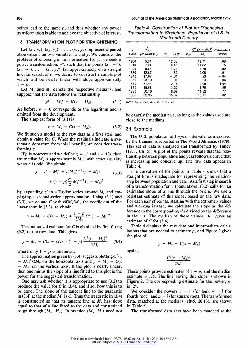
Table 4. Construction of Plot for Diagnosing Transformation to Straighten; Population of U.S. in

Nineteenth Century

y x Pop C2 (x - Mx)2 Estimated

Date (millions) y - my - C (x - Mx) 2My Slope

1800 5.31 12.63 18.71 .68 1810 7.24 8.46 11.32 .75 1820 9.64 4.76 5.78 .82 1830 12.87 1.89 2.08 .91 1840 17.07 -.01 .23 -.04 1850 23.19 .01 .23 .04 1860 31.44 2.16 2.08 1.04 1870 38.58 3.20 5.78 .55 1880 50.16 8.68 11.32 .77 1890 62.95 15.37 18.71 .82

NOTE: MX = 1845, My = 20.13, C = .61

be exactly the median pair, as long as the values used are close to the medians.

3.1 Example

The U.S. population at 10-year intervals, as measured by the Census, is reported in The World Almanac (1978). This set of data is analyzed and transformed by Tukey (1977, Ch. 5). A plot of the points reveals that the relationship between population and year follows a curve that is increasing and concave up. The raw data appear in Table 4.

The curvature of the points in Table 4 shows that a straight line is inadequate for representing the relationship between population and year. As a first step in search of a transformation for y (population), (3.2) calls for an estimated slope of a line through the origin. We use a resistant estimate of this slope, based on the raw data. For each pair of points, starting with the extreme x values and working inward, we calculate the slope as the difference in the corresponding y's divided by the difference in the x's. The median of these values, .61, gives an estimate of C for (3.4).

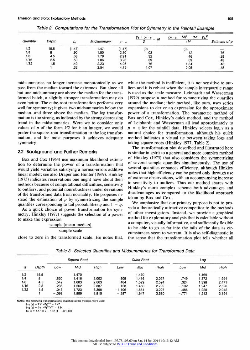
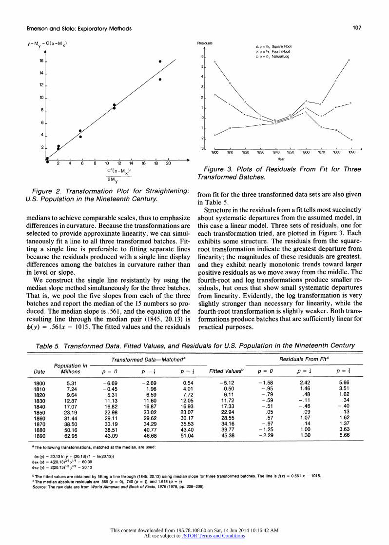
Table 4 displays the raw data and intermediate calculations that are needed to estimate p, and Figure 2 gives the plot of

y - - C(x - MX)

against

C2(X _ MX)2

2My

These points provide estimates of 1 - p, and the median estimate is .76. The line having this slope is shown in Figure 2. The corresponding estimate for the power, p, is .24.

We consider the powers p = 0 (for log), p = X (for fourth root), and p = 2 (for square root). The transformed data, matched at the medians (1845, 20.13), are shown in Table 5.

The transformed data sets have been matched at the



Emerson and Stoto: Exploratory Methods 107

16

14

12

10

8

6

40

2

2 4 6 8 10 12 14 16 18 20

C2(x-M )2

2My

Figure 2. Transformation Plot for Straightening: U.S. Population in the Nineteenth Century.

medians to achieve comparable scales, thus to emphasize differences in curvature. Because the transformations are selected to provide approximate linearity, we can simultaneously fit a line to all three transformed batches. Fit- ting a single line is preferable to fitting separate lines because the residuals produced with a single line display differences among the batches in curvature rather than in level or slope.

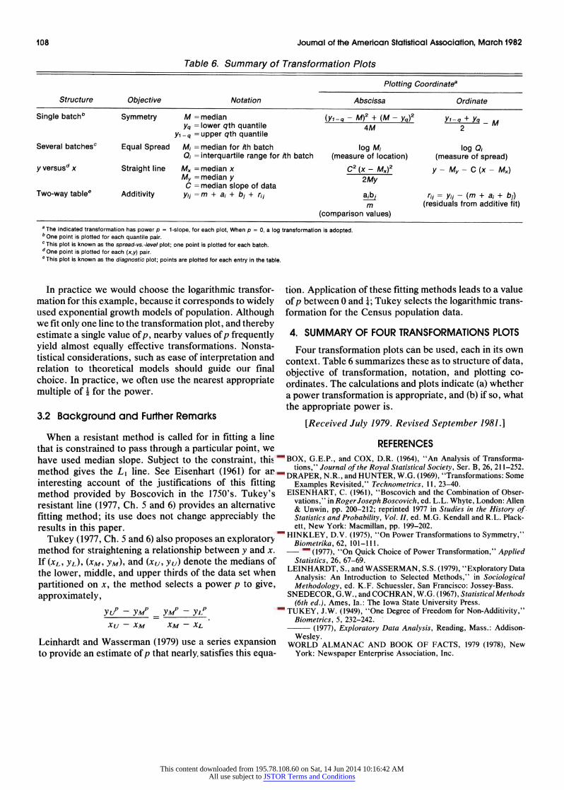
We construct the single line resistantly by using the median slope method simultaneously for the three batches. That is, we pool the five slopes from each of the three batches and report the median of the 15 numbers so produced. The median slope is .561, and the equation of the resulting line through the median pair (1845, 20.13) is +(y) = .561x - 1015. The fitted values and the residuals

Residuals Ap = 1/2, Square Root x p = 1/4, Fourth Root

6 o p = 0, Natural Log

A A~~~~~~~~~~~~

5 \/

0 x\-> HA^,= A 1 o-

0

2

3 L I I I I

1800 1810 1820 1830 1840 1850 1860 1870 1880 1890

Year

Figure 3. Plots of Residuals From Fit for Three Transformed Batches.

from fit for the three transformed data sets are also given in Table 5.

Structure in the residuals from a fit tells most succinctly about systematic departures from the assumed model, in this case a linear model. Three sets of residuals, one for each transformation tried, are plotted in Figure 3. Each exhibits some structure. The residuals from the square- root transformation indicate the greatest departure from linearity; the magnitudes of these residuals are greatest, and they exhibit nearly monotonic trends toward larger positive residuals as we move away from the middle. The fourth-root and log transformations produce smaller residuals, but ones that show small systematic departures from linearity. Evidently, the log transformation is very slightly stronger than necessary for linearity, while the fourth-root transformation is slightly weaker. Both transformations produce batches that are sufficiently linear for practical purposes.

Table 5. Transformed Data, Fitted Values, and Residuals for U.S. Population in the Nineteenth Century

Transformed Data-Matcheda Residuals From Fitc Population in

Date Millions p=O p= p = a Fitted Valuesb p p== 4 2

1800 5.31 -6.69 -2.69 0.54 -5.12 -1.58 2.42 5.66 1810 7.24 -0.45 1.96 4.01 0.50 -.95 1.46 3.51 1820 9.64 5.31 6.59 7.72 6.11 -.79 .48 1.62 1830 12.87 11.13 11.60 12.05 11.72 -.59 -.11 .34 1840 17.07 16.82 16.87 16.93 17.33 -.51 -.46 -.40 1850 23.19 22.98 23.02 23.07 22.94 .05 .09 .13 1860 31.44 29.11 29.62 30.17 28.55 .57 1.07 1.62 1870 38.50 33.19 34.29 35.53 34.16 -.97 .14 1.37 1880 50.16 38.51 40.77 43.40 39.77 -1.25 1.00 3.63 1890 62.95 43.09 46.68 51.04 45.38 -2.29 1.30 5.66

aThe following transformations, matched at the median, are used:

4o (y) = 20.13 In y + (20.13) (1 - ln(20.13))

,1/4 (y) = 4(20.13)314 y"4 - 60.39

+1/2 (y) = 2(20.13)112 y1"2 - 20.13

bThe fitted values are obtained by fitting a line through (1845, 20.13) using median slope for three transformed batches. The line is f(x) = 0.561 x - 1015.

cThe median absolute residuals are .869 (p = 0), .740 (p = )), and 1.618 (p = 1) Source: The raw data are from World Almanac and Book of Facts, 1979 (1978, pp. 208-209).




Table 6. Summary of Transformation Plots

Plotting Coordinatea

Structure Objective Notation Abscissa Ordinate

Single batchb Symmetry M =median (Yigq - M)2 + (M - yq)2 Yi-q + Yq - M yq= lower qth quantile 4M 2

Yi-q =upper qth quantile Several batchesc Equal Spread Mi =median for ith batch log Mj log Qj

Q0 = interquartile range for ith batch (measure of location) (measure of spread) y versusdx Straight line MX =median x C2 (x - MX)2 y - - C (x - Mx)

My =median y My C = median slope of data

Two-way tablee Additivity y,j = m + a, + bj + rij a,b1 r,j = yij - (m + a, + bj) m (residuals from additive fit)

(comparison values)

a The indicated transformation has power p = 1-slope, for each plot, When p = 0, a log transformation is adopted. b One point is plotted for each quantile pair. c This plot is known as the spread-vs.-level plot; one point is plotted for each batch. d One point is plotted for each (xy) pair. e This plot is known as the diagnostic plot; points are plotted for each entry in the table.

In practice we would choose the logarithmic transformation for this example, because it corresponds to widely used exponential growth models of population. Although we fit only one line to the transformation plot, and thereby estimate a single value of p, nearby values of p frequently yield almost equally effective transformations. Nonsta- tistical considerations, such as ease of interpretation and relation to theoretical models should guide our final choice. In practice, we often use the nearest appropriate multiple of 2 for the power.

3.2 Background and Further Remarks

When a resistant method is called for in fitting a line that is constrained to pass through a particular point, we have used median slope. Subject to the constraint, this method gives the LI line. See Eisenhart (1961) for an interesting account of the justifications of this fitting method provided by Boscovich in the 1750's. Tukey's resistant line (1977, Ch. 5 and 6) provides an alternative fitting method; its use does not change appreciably the results in this paper.

Tukey (1977, Ch. 5 and 6) also proposes an exploratory method for straightening a relationship between y and x. If (XL, YL), (XM, YM), and (xu, y.u) denote the medians of the lower, middle, and upper thirds of the data set when partitioned on x, the method selects a power p to give, approximately,

y up -YMP _ YMP - YLP

XU - XM XM - XL

Leinhardt and Wasserman (1979) use a series expansion to provide an estimate of p that nearly, satisfies this equa-

tion. Application of these fitting methods leads to a value of p between 0 and 1; Tukey selects the logarithmic transformation for the Census population data.

4. SUMMARY OF FOUR TRANSFORMATIONS PLOTS

Four transformation plots can be used, each in its own context. Table 6 summarizes these as to structure of data, objective of transformation, notation, and plotting co- ordinates. The calculations and plots indicate (a) whether a power transformation is appropriate, and (b) if so, what the appropriate power is.

[Received July 1979. Revised September 1981.]

REFERENCES BOX, G.E.P., and COX, D.R. (1964), "An Analysis of Transforma-

tions," Journal of the Royal Statistical Society, Ser. B, 26, 211-252. DRAPER, N.R., and HUNTER, W.G. (1969), "Transformations: Some

Examples Revisited," Technometrics, 11, 23-40. EISENHART, C. (1961), "Boscovich and the Combination of Obser-

vations," in Roger Joseph Boscovich, ed. L.L. Whyte, London: Allen & Unwin, pp. 200-212; reprinted 1977 in Studies in the History of Statistics and Probability, Vol. II, ed. M.G. Kendall and R.L. Plack- ett, New York: Macmillan, pp. 199-202.

HINKLEY, D.V. (1975), "On Power Transformations to Symmetry," Biometrika, 62, 101-111.

(1977), "On Quick Choice of Power Transformation," Applied Statistics, 26, 67-69.

LEINHARDT, S., and WASSERMAN, S.S. (1979), "Exploratory Data Analysis: An Introduction to Selected Methods," in Sociological Methodology, ed. K.F. Schuessler, San Francisco: Jossey-Bass.

SNEDECOR, G.W., and COCHRAN, W.G. (1967), Statistical Methods (6th ed.), Ames, Ia.: The Iowa State University Press.

TUKEY, J.W. (1949), "One Degree of Freedom for Non-Additivity," Biometrics, 5, 232-242.

(1977), Exploratory Data Analysis, Reading, Mass.: Addison- Wesley.

WORLD ALMANAC AND BOOK OF FACTS, 1979 (1978), New York: Newspaper Enterprise Association, Inc.



exploratory methods for choosing power transformations

Documents