Exploratory Analysis of Suburban Land Coverand Population Density in the U.S.A.

Francesca Pozzi 1 and Christopher Small 2

1CIESINColumbia University

Palisades, NY 10964 USAfpozzi@ciesin.columbia.edu

2Lamont Doherty Earth ObservatoryColumbia University

Palisades, NY 10964 USAsmall@LDEO.columbia.edu

Reprinted from:

IEEE/ISPRS joint Workshop on Remote Sensing and Data Fusion over Urban Areas,Paper 35

Rome, Italy8-9 November, 2001

Copyright © 2001 IEEE. Reprinted from IEEE/ISPRS joint Workshop on RemoteSensing and Data Fusion over Urban Areas. This material is posted here with permission ofthe IEEE. Internal or personal use of this material is permitted. However, permission toreprint/republish this material for advertising or promotional purposes or for creating newcollective works for resale or redistribution must be obtained from the IEEE by sending ablank email message to pubs-permissions@ieee.org. By choosing to view this document,you agree to all provisions of the copyright laws protecting it.

1

Exploratory Analysis of Suburban Land Cover andPopulation Density in the U.S.A.

Francesca Pozzi, Christopher Small

Abstract— The objective of this study is to investigate theconsistency of “suburban” population densities and landcovers. We analyzed population density, extracted fromthe census, and vegetation abundance, derived from Land-sat imagery, taking six cities in the U.S.A. as contrastingexamples. Combining population density and areal vege-tation abundance estimates yields univariate and bivariatedistributions for the two variables. We quantify the rela-tionship between population density and vegetation fractionin Atlanta, Chicago, Los Angeles, New York, Phoenix andSeattle. A bimodal distribution of population density inthe U.S.A. suggests that it may be possible to characterize“suburban” areas on the basis of population density between100 and 10,000 people/km2. The maximum areal vegetationcover diminishes linearly with the Log10 of population den-sity in cities with large density ranges.

Keywords— Suburban, Population Density, VegetationFraction, Land Cover

I. Introduction

Suburban areas in the U.S.A.are often perceived as thegreener “residential areas on the outskirts of a city or alarge town” [1], socially and economically dependent onlarge cities. Suburbs have been given consideration in thepast decade, given the close connections with cities andthe negative consequences associated with urban sprawl.These consequences include loss of agricultural land andnatural vegetation, increased traffic congestion and associ-ated degradation of air quality.

According to the U.S.Census Bureau [2], between 1995and 1996 more than 2 million people moved from U.S.A.cities and from non-metropolitan areas into the “suburbs”.In the same report suburbs are defined as “all territorywithin an Metropolitan Statistical Areas (MSA) but out-side of a central city”. Although this definition is intuitiveand easily understandable, there appears to be no consis-tent or formal characterization of suburban areas in termsof physical or socioeconomic characteristics.

In recent years, many authors have considered the re-lationship between population characteristics and environ-mental variables, but their interests and goals are differentfrom the ones presented in this paper. Examples are [3],[4], [5], where the authors presented studies of integrationof population and land cover for quality of life assessmentor improvement of land cover classification. Studies [6]and [7] considered population and vegetation to better un-derstand urban dynamics. Other authors analyzed landcover change related to population change and its impacts

F. Pozzi is a research associate at the Center for International EarthScience Information Network (CIESIN) of Columbia University. E-mail: fpozzi@ciesin.columbia.edu

C. Small is a researcher at the Lamont Doherty Earth Observatoryof Columbia University. E-mail: small@LDEO.columbia.edu

on the surrounding natural areas [8]. Approaches more fo-cused on the correlation between socioeconomic variables,such as population count and housing density, and landcover are presented in [9] and [10].

The above mentioned studies focused mainly on the in-tegration of population and land cover data and on singlecase studies. To our knowledge, no study has yet been per-formed to examine the demographic and land cover char-acteristics of suburban areas and their consistency acrossdifferent physiographic environments.

The purpose of this paper is to investigate the questionof whether suburban areas can be defined based on demo-graphic and physical characteristics, specifically populationdensity and vegetation cover. Based on the expectationthat suburban areas are greener than urban centers, andthat the predominant suburban land cover is vegetation,we attempt to quantify the extent to which suburban ar-eas are vegetated in different U.S.A. cities. We considersuburban areas based on population density and on appar-ent spectral reflectance using Landsat data to quantify therelationship between the two variables looking at the citiesof Atlanta, Chicago, Los Angeles, New York, Phoenix andSeattle.

II. Data

Given the purpose of the study, the six cities we consid-ered present very different characteristics, in terms of geo-graphic location and spatial structure and dynamics. Wechose cities located in a temperate climate, both in a de-ciduous forest biome (New York, Chicago, Atlanta) and inan evergreen forest biome (Seattle) and cities located in anarid or semi-arid climate (Los Angeles and Phoenix). Wealso included cities that have been among the most fast-growing of the past decades in the U.S.A. (Phoenix andSeattle), and cities that have experienced rapid growth inthe past and now are characterized by large population(New York, Chicago, Los Angeles).

A. Population Density

We calculated population density from the 1990 U.S.Census Bureau population counts at the block level, thelowest in the U.S. census structural hierarchy. These dataare available separately as spatial data (Topologically In-tegrated Geographic Encoding and Referencing system -TIGERr) and tabular data (Summary Tape Files-STFs)for each county in the U.S.A.. In this study we consideredpopulation density, expressed in persons/km2. For eachcity we selected one or more counties containing the Cen-tered Business District (CBD) and the surrounding sub-

2

urbs. This resulted in the selection of the following coun-ties, for which we then created a smaller subset concordantwith Landsat coverage (area reported in parenthesis):• Atlanta: DeKalb and Fulton (900 km2);• Chicago: Cook (950 km2);• Los Angeles: Los Angeles (3100 km2);• New York Metropolitan Area: Bronx, Kings, NewYork, Queens, Richmond, Bergen, Essex, Hudson, Passaic,Nassau, Rockland, Westchester (2000 km2);• Phoenix: Maricopa (4700 km2);• Seattle: King (3200 km2).

B. Vegetation Fraction

The characteristic spatial scale and the spectral variabil-ity of urban and suburban land cover poses serious prob-lems for traditional image classification algorithms. In ar-eas where the reflectance spectra of the land cover varyappreciably at scales comparable to, or smaller than, theGround Instantaneous Field Of View (GIFOV) of mostsatellite sensors, the spectral reflectance of a individualpixel will generally not resemble the reflectance of a singleland cover class but rather a mixture of the reflectances oftwo or more classes present within the GIFOV. Becausethey are combinations of spectrally distinct land covertypes, mixed pixels in urban areas are frequently misclas-sified as other land cover classes. Similarly, the definitionof an “urban” spectral class will usually incorporate pixelsof other non-urban classes.

If an urban area contains significant amounts of vege-tation then the reflectance spectra measured by the sen-sor will be influenced by the reflectance characteristics ofthe vegetation. Macroscopic combinations of homogeneous“endmember” materials within the GIFOV produce a com-posite reflectance spectrum that can often be described asa linear combination of the spectra of the endmembers [11].If mixing between the endmember spectra is predominantlylinear and the endmembers are known a priori, it may bepossible to “unmix” individual pixels by estimating thefraction of each endmember in the composite reflectanceof a mixed pixel [12], [13].

Analysis of Landsat TM imagery suggests that the spec-tral reflectance of many urban areas can be described aslinear mixing of three distinct spectral endmembers [14],[15]. Principal component analysis of urban reflectanceconsistently yield eigenvalue distributions suggesting thatthe majority of scene variance is contained within a two di-mensional mixing plane. The triangular distribution in themixing space defined by the principal components bears asimilarity to the well known Tasseled Cap distribution dis-covered by [16]. The feature space distributions are similarin the sense that both contain a vegetation endmemberthat is distinct from a mixing continuum between high andlow albedo endmembers.

The spectral endmembers determined for the areas inves-tigated here correspond to low albedo (e.g. water, shadow,roofing), high albedo (e.g. cloud, sand, roofing) and veg-etation. The strong visible absorption and infrared re-flectance that is characteristic of vegetation is sufficiently

distinct from the spectrally flat reflectance of the low andhigh albedo endmembers to allow the three components tobe “unmixed” by inverting a simple three component lin-ear mixing model [14]. The result of the unmixing is aset of fraction images showing the areal percentages, givenas fractions between 0 and 1, of each endmember presentwithin each pixel. Analysis of Landsat, Ikonos and AVIRISimagery of several urban/suburban areas shows that athree component linear mixing model provides stable, con-sistent estimates of vegetation fraction for both constrainedand unconstrained inversions using three different endmem-ber selection methods [15]. Vegetation fraction estimatesderived from Landsat TM data were validated with aeralvegetation fractions calculated from 2 m aerial photogra-phy and generally showed agreement to within 10% [14]The vegetation fraction estimates given here were derivedfrom Landsat TM and validated with Ikonos MSI imagery.

III. Analysis and Results

The first step of the analysis was to quantify the distribu-tion of population density across the entire United Statesto estimate whether rural, urban and suburban areas areclearly discernible based on population density. The dis-tribution of people as a function of population density forthe U.S.A. in 1990 is bimodal (Figure 1) [17]. The modesrepresent the spatially concentrated settlements near citiesand the spatially dispersed settlements farther from cities.The larger mode has a distinct break in slope near 10,000people/km2, and a short, high density tail. This tail corre-sponds to the high density cores of large cities. For the pur-poses of this study we consider suburban areas to be char-acterized by population density between 100 and 10,000people/km2.

To perform the study on the six cities, spatial and tab-ular data from the Census were initially aggregated basedon the block numeric codes for each county. The result-ing vector layers were then projected to UTM coordinates,

Fig. 1. Histogram of the Population Density for the U.S.A., showingalso the distribution for Eastern U.S.A. (East of the 90 ◦ W, blackline) and for Western U.S.A.(grey line).

3

Fig. 2. Population Density and Vegetation Fraction at full resolution for part of New York Metropolitan Area. Black areas represent nodata for population density and no vegetation (water) for the vegetation fraction.

rasterized to a 30 m grid and coregistered to the Landsatdata. To quantify the relationship between population den-sity and vegetation fraction, we produced bivariate distri-butions of people and land area as functions of populationdensity and vegetation fraction. The bivariate populationdistributions are shown with population density and vege-tation fraction for each city in Figure 3. We then summedthe bivariate distributions to produce marginal distribu-tions of people as functions of population density and veg-etation fraction for each city (Figure 4).

IV. Discussion

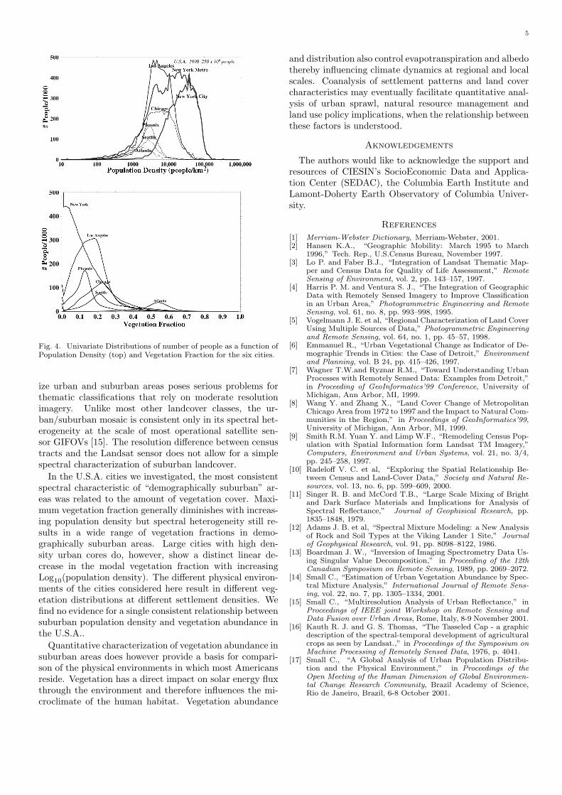
In the six cities we studied there appears to be a patternfor suburban areas, both in terms of population density andvegetation fractions. The population density histograms,calculated for the counties listed in II-A, show the subur-ban peak characteristic of the entire U.S.A. with Atlantaand New York at the extremes (Figure 4. The vegetationfraction histograms also show a consistent pattern, withpeaks varying between about 0.1 and 0.55. The cities withlarge urban core also present a smaller peak for vegetationfractions less than 0.01. Prominent exceptions are Atlanta,which has a symmetric distribution centered on higher val-ues (0.5 to 0.6) and New York, which has a long tailedmonotonic distribution, with a peak at less than 0.1.

The differences between the physiographic environmentsand the urban structures for the six cities are such thatthe peaks of the bivariate histograms are spread acrossa range of population densities and vegetation fractions.Nonetheless a consistent sub-linear relationship is seen forthe largest cities (New York, Chicago and Los Angeles).These three cities have similar density distributions, with

comparable peak values and with vegetation fractions lin-early decreasing with Log10(Population Density). Phoenixand Seattle have the most similar population density dis-tributions, but their vegetation fraction distributions aredifferent, due to their arid and humid climates. The bi-variate distributions for these two cities are more isotropicthan the larger cities, with Phoenix containing large inhab-ited unvegetated areas and Seattle characterized by largeuninhabited and densely vegetated areas. Atlanta, on theother hand, presents a more uniform distribution, with lit-tle variations in either vegetation fraction and populationdensity.

V. Conclusions

The objective of this study was to investigate the consis-tency of “suburban” settlement patterns, based on the rela-tionship between population density and land cover amongdifferent cities in the U.S.A.. The principal conclusion ofthis study is that the population density distribution in theU.S.A. may provide a demographic basis for distinguishingurban, suburban and rural areas. The block level popula-tion density distribution for the entire U.S.A. shows twodistinct modes corresponding to moderate density (100 to10,000 people/km2) settlements surrounding higher den-sity urban cores and to low density settlements (less than100 people/km2) dispersed throughout the country. Thehigh density (more than 10,000 people/km2) cores corre-spond to a distinct tail delineated by a break in slope onthe moderate density ”suburban” mode. This demographicclassification would place 71% of Americans in suburbanareas, 25% in rural areas and 3% in urban areas in 1990.

The wide variety of land use classes that character-

4

Fig. 3. Spatial Distributions of Population and Vegetation. Combining population density with vegetation fraction yields a demographicclassification, where rural population densities are shown in blue, urban in red and suburban in green. Different shades of green correspondto different amounts of vegetation. Note the similarity of the peaks in the bivariate distributions for Chicago, New York and Los Angeles.Full resolution images are available at www.LDEO.columbia.edu/˜ small/Urban.html

5

Fig. 4. Univariate Distributions of number of people as a function ofPopulation Density (top) and Vegetation Fraction for the six cities.

ize urban and suburban areas poses serious problems forthematic classifications that rely on moderate resolutionimagery. Unlike most other landcover classes, the ur-ban/suburban mosaic is consistent only in its spectral het-erogeneity at the scale of most operational satellite sen-sor GIFOVs [15]. The resolution difference between censustracts and the Landsat sensor does not allow for a simplespectral characterization of suburban landcover.

In the U.S.A. cities we investigated, the most consistentspectral characteristic of “demographically suburban” ar-eas was related to the amount of vegetation cover. Maxi-mum vegetation fraction generally diminishes with increas-ing population density but spectral heterogeneity still re-sults in a wide range of vegetation fractions in demo-graphically suburban areas. Large cities with high den-sity urban cores do, however, show a distinct linear de-crease in the modal vegetation fraction with increasingLog10(population density). The different physical environ-ments of the cities considered here result in different veg-etation distributions at different settlement densities. Wefind no evidence for a single consistent relationship betweensuburban population density and vegetation abundance inthe U.S.A..

Quantitative characterization of vegetation abundance insuburban areas does however provide a basis for compari-son of the physical environments in which most Americansreside. Vegetation has a direct impact on solar energy fluxthrough the environment and therefore influences the mi-croclimate of the human habitat. Vegetation abundance

and distribution also control evapotranspiration and albedothereby influencing climate dynamics at regional and localscales. Coanalysis of settlement patterns and land covercharacteristics may eventually facilitate quantitative anal-ysis of urban sprawl, natural resource management andland use policy implications, when the relationship betweenthese factors is understood.

Aknowledgements

The authors would like to acknowledge the support andresources of CIESIN’s SocioEconomic Data and Applica-tion Center (SEDAC), the Columbia Earth Institute andLamont-Doherty Earth Observatory of Columbia Univer-sity.

References

[1] Merriam-Webster Dictionary, Merriam-Webster, 2001.[2] Hansen K.A., “Geographic Mobility: March 1995 to March

1996,” Tech. Rep., U.S.Census Bureau, November 1997.[3] Lo P. and Faber B.J., “Integration of Landsat Thematic Map-

per and Census Data for Quality of Life Assessment,” RemoteSensing of Environment, vol. 2, pp. 143–157, 1997.

[4] Harris P. M. and Ventura S. J., “The Integration of GeographicData with Remotely Sensed Imagery to Improve Classificationin an Urban Area,” Photogrammetric Engineering and RemoteSensing, vol. 61, no. 8, pp. 993–998, 1995.

[5] Vogelmann J. E. et al, “Regional Characterization of Land CoverUsing Multiple Sources of Data,” Photogrammetric Engineeringand Remote Sensing, vol. 64, no. 1, pp. 45–57, 1998.

[6] Emmanuel R., “Urban Vegetational Change as Indicator of De-mographic Trends in Cities: the Case of Detroit,” Environmentand Planning, vol. B 24, pp. 415–426, 1997.

[7] Wagner T.W.and Ryznar R.M., “Toward Understanding UrbanProcesses with Remotely Sensed Data: Examples from Detroit,”in Proceeding of GeoInformatics’99 Conference, University ofMichigan, Ann Arbor, MI, 1999.

[8] Wang Y. and Zhang X., “Land Cover Change of MetropolitanChicago Area from 1972 to 1997 and the Impact to Natural Com-munities in the Region,” in Proceedings of GeoInformatics’99,University of Michigan, Ann Arbor, MI, 1999.

[9] Smith R.M. Yuan Y. and Limp W.F., “Remodeling Census Pop-ulation with Spatial Information form Landsat TM Imagery,”Computers, Environment and Urban Systems, vol. 21, no. 3/4,pp. 245–258, 1997.

[10] Radeloff V. C. et al, “Exploring the Spatial Relationship Be-tween Census and Land-Cover Data,” Society and Natural Re-sources, vol. 13, no. 6, pp. 599–609, 2000.

[11] Singer R. B. and McCord T.B., “Large Scale Mixing of Brightand Dark Surface Materials and Implications for Analysis ofSpectral Reflectance,” Journal of Geophisical Research, pp.1835–1848, 1979.

[12] Adams J. B. et al, “Spectral Mixture Modeling: a New Analysisof Rock and Soil Types at the Viking Lander 1 Site,” Journalof Geophysical Research, vol. 91, pp. 8098–8122, 1986.

[13] Boardman J. W., “Inversion of Imaging Spectrometry Data Us-ing Singular Value Decomposition,” in Proceeding of the 12thCanadian Symposium on Remote Sensing, 1989, pp. 2069–2072.

[14] Small C., “Estimation of Urban Vegetation Abundance by Spec-tral Mixture Analysis,” International Journal of Remote Sens-ing, vol. 22, no. 7, pp. 1305–1334, 2001.

[15] Small C., “Multiresolution Analysis of Urban Reflectance,” inProceedings of IEEE joint Workshop on Remote Sensing andData Fusion over Urban Areas, Rome, Italy, 8-9 November 2001.

[16] Kauth R. J. and G. S. Thomas, “The Tasseled Cap - a graphicdescription of the spectral-temporal development of agriculturalcrops as seen by Landsat.,” in Proceedings of the Symposium onMachine Processing of Remotely Sensed Data, 1976, p. 4041.

[17] Small C., “A Global Analysis of Urban Population Distribu-tion and the Physical Environment,” in Proceedings of theOpen Meeting of the Human Dimension of Global Environmen-tal Change Research Community, Brazil Academy of Science,Rio de Janeiro, Brazil, 6-8 October 2001.