experiment of design
TRANSCRIPT

Introduction to Design and Analysis of Experiments with the SAS
System
(Stat 7010 Lecture Notes)
Asheber AbebeDiscrete and Statistical Sciences
Auburn University

ii

Contents
1 Completely Randomized Design 11.1 Introduction . . . . . . . . . . . . . . . . . . . . . . . . . . . . . . . . . . . . . . . . . . . . . . 11.2 The Fixed Effects Model . . . . . . . . . . . . . . . . . . . . . . . . . . . . . . . . . . . . . . . 2
1.2.1 Decomposition of the Total Sum of Squares . . . . . . . . . . . . . . . . . . . . . . . . 21.2.2 Statistical Analysis . . . . . . . . . . . . . . . . . . . . . . . . . . . . . . . . . . . . . . 31.2.3 Comparison of Individual Treatment Means . . . . . . . . . . . . . . . . . . . . . . . . 5
1.3 The Random Effects Model . . . . . . . . . . . . . . . . . . . . . . . . . . . . . . . . . . . . . 101.4 More About the One-Way Model . . . . . . . . . . . . . . . . . . . . . . . . . . . . . . . . . . 18
1.4.1 Model Adequacy Checking . . . . . . . . . . . . . . . . . . . . . . . . . . . . . . . . . 181.4.2 Some Remedial Measures . . . . . . . . . . . . . . . . . . . . . . . . . . . . . . . . . . 23
2 Randomized Blocks 252.1 The Randomized Complete Block Design . . . . . . . . . . . . . . . . . . . . . . . . . . . . . 25
2.1.1 Introduction . . . . . . . . . . . . . . . . . . . . . . . . . . . . . . . . . . . . . . . . . 252.1.2 Decomposition of the Total Sum of Squares . . . . . . . . . . . . . . . . . . . . . . . . 262.1.3 Statistical Analysis . . . . . . . . . . . . . . . . . . . . . . . . . . . . . . . . . . . . . . 272.1.4 Relative Efficiency of the RCBD . . . . . . . . . . . . . . . . . . . . . . . . . . . . . . 292.1.5 Comparison of Treatment Means . . . . . . . . . . . . . . . . . . . . . . . . . . . . . . 302.1.6 Model Adequacy Checking . . . . . . . . . . . . . . . . . . . . . . . . . . . . . . . . . 302.1.7 Missing Values . . . . . . . . . . . . . . . . . . . . . . . . . . . . . . . . . . . . . . . . 36
2.2 The Latin Square Design . . . . . . . . . . . . . . . . . . . . . . . . . . . . . . . . . . . . . . 382.2.1 Statistical Analysis . . . . . . . . . . . . . . . . . . . . . . . . . . . . . . . . . . . . . . 392.2.2 Missing Values . . . . . . . . . . . . . . . . . . . . . . . . . . . . . . . . . . . . . . . . 412.2.3 Relative Efficiency . . . . . . . . . . . . . . . . . . . . . . . . . . . . . . . . . . . . . . 412.2.4 Replicated Latin Square . . . . . . . . . . . . . . . . . . . . . . . . . . . . . . . . . . . 42
2.3 The Graeco-Latin Square Design . . . . . . . . . . . . . . . . . . . . . . . . . . . . . . . . . . 482.4 Incomplete Block Designs . . . . . . . . . . . . . . . . . . . . . . . . . . . . . . . . . . . . . . 51
2.4.1 Balanced Incomplete Block Designs (BIBD’s) . . . . . . . . . . . . . . . . . . . . . . . 512.4.2 Youden Squares . . . . . . . . . . . . . . . . . . . . . . . . . . . . . . . . . . . . . . . . 552.4.3 Other Incomplete Designs . . . . . . . . . . . . . . . . . . . . . . . . . . . . . . . . . . 55
3 Factorial Designs 573.1 Introduction . . . . . . . . . . . . . . . . . . . . . . . . . . . . . . . . . . . . . . . . . . . . . . 573.2 The Two-Factor Factorial Design . . . . . . . . . . . . . . . . . . . . . . . . . . . . . . . . . . 59
3.2.1 The Fixed Effects Model . . . . . . . . . . . . . . . . . . . . . . . . . . . . . . . . . . . 603.2.2 Random and Mixed Models . . . . . . . . . . . . . . . . . . . . . . . . . . . . . . . . . 70
3.3 Blocking in Factorial Designs . . . . . . . . . . . . . . . . . . . . . . . . . . . . . . . . . . . . 753.4 The General Factorial Design . . . . . . . . . . . . . . . . . . . . . . . . . . . . . . . . . . . . 79
iii

iv CONTENTS
4 2k and 3k Factorial Designs 834.1 Introduction . . . . . . . . . . . . . . . . . . . . . . . . . . . . . . . . . . . . . . . . . . . . . . 834.2 The 2k Factorial Design . . . . . . . . . . . . . . . . . . . . . . . . . . . . . . . . . . . . . . . 83
4.2.1 The 22 Design . . . . . . . . . . . . . . . . . . . . . . . . . . . . . . . . . . . . . . . . 834.2.2 The 23 Design . . . . . . . . . . . . . . . . . . . . . . . . . . . . . . . . . . . . . . . . 864.2.3 The General 2k Design . . . . . . . . . . . . . . . . . . . . . . . . . . . . . . . . . . . . 894.2.4 The Unreplicated 2k Design . . . . . . . . . . . . . . . . . . . . . . . . . . . . . . . . . 90
4.3 The 3k Design . . . . . . . . . . . . . . . . . . . . . . . . . . . . . . . . . . . . . . . . . . . . 99
5 Repeated Measurement Designs 1015.1 Introduction . . . . . . . . . . . . . . . . . . . . . . . . . . . . . . . . . . . . . . . . . . . . . . 101
5.1.1 The Mixed RCBD . . . . . . . . . . . . . . . . . . . . . . . . . . . . . . . . . . . . . . 1015.2 One-Way Repeated Measurement Designs . . . . . . . . . . . . . . . . . . . . . . . . . . . . . 103
5.2.1 The Huynh-Feldt Sphericity (S) Structure . . . . . . . . . . . . . . . . . . . . . . . . . 1045.2.2 The One-Way RM Design : (S) Structure . . . . . . . . . . . . . . . . . . . . . . . . . 1045.2.3 One-way RM Design : General . . . . . . . . . . . . . . . . . . . . . . . . . . . . . . . 107
5.3 Two-Way Repeated Measurement Designs . . . . . . . . . . . . . . . . . . . . . . . . . . . . . 109
6 More on Repeated Measurement Designs 1296.1 Trend Analyses in One- and Two-way RM Designs . . . . . . . . . . . . . . . . . . . . . . . . 129
6.1.1 Regression Components of the Between Treatment SS (SSB) . . . . . . . . . . . . . . 1296.1.2 RM Designs . . . . . . . . . . . . . . . . . . . . . . . . . . . . . . . . . . . . . . . . . . 134
6.2 The Split-Plot Design . . . . . . . . . . . . . . . . . . . . . . . . . . . . . . . . . . . . . . . . 1406.3 Crossover Designs . . . . . . . . . . . . . . . . . . . . . . . . . . . . . . . . . . . . . . . . . . 1466.4 Two-Way Repeated Measurement Designs with Repeated Measures on Both Factors . . . . . 151
7 Introduction to the Analysis of Covariance 1577.1 Simple Linear Regression . . . . . . . . . . . . . . . . . . . . . . . . . . . . . . . . . . . . . . 157
7.1.1 Estimation : The Method of Least Squares . . . . . . . . . . . . . . . . . . . . . . . . 1577.1.2 Partitioning the Total SS . . . . . . . . . . . . . . . . . . . . . . . . . . . . . . . . . . 1587.1.3 Tests of Hypotheses . . . . . . . . . . . . . . . . . . . . . . . . . . . . . . . . . . . . . 158
7.2 Single Factor Designs with One Covariate . . . . . . . . . . . . . . . . . . . . . . . . . . . . . 1627.3 ANCOVA in Randomized Complete Block Designs . . . . . . . . . . . . . . . . . . . . . . . . 1667.4 ANCOVA in Two-Factor Designs . . . . . . . . . . . . . . . . . . . . . . . . . . . . . . . . . . 1707.5 The Johnson-Neyman Technique: Heterogeneous Slopes . . . . . . . . . . . . . . . . . . . . . 174
7.5.1 Two Groups, One Covariate . . . . . . . . . . . . . . . . . . . . . . . . . . . . . . . . . 1747.5.2 Multiple Groups, One Covariate . . . . . . . . . . . . . . . . . . . . . . . . . . . . . . 180
8 Nested Designs 1818.1 Nesting in the Design Structure . . . . . . . . . . . . . . . . . . . . . . . . . . . . . . . . . . . 1818.2 Nesting in the Treatment Structure . . . . . . . . . . . . . . . . . . . . . . . . . . . . . . . . . 185

Chapter 1
Completely Randomized Design
1.1 Introduction
Suppose we have an experiment which compares k treatments or k levels of a single factor. Suppose we have nexperimental units to be included in the experiment. We can assign the first treatment to n1 units randomlyselected from among the n, assign the second treatment to n2 units randomly selected from the remainingn−n1 units, and so on until the kth treatment is assigned to the final nk units. Such an experimental designis called a completely randomized design (CRD).
We shall describe the observations using the linear statistical model
yij = µ + τi + εij , i = 1, · · · , k, j = 1, · · · , ni , (1.1)
where
• yij is the jth observation on treatment i,
• µ is a parameter common to all treatments (overall mean),
• τi is a parameter unique to the ith treatment (ith treatment effect), and
• εij is a random error component.
In this model the random errors are assumed to be normally and independently distributed with mean zeroand variance σ2, which is assumed constant for all treatments. The model is called the one-way classificationanalysis of variance (one-way ANOVA).
The typical data layout for a one-way ANOVA is shown below:
Treatment1 2 · · · ky11 y21 yk1
y11 y21 yk1
......
...y1n1 y2n2 yknk
The model in Equation (1.1) describes two different situations :
1. Fixed Effects Model : The k treatments could have been specifically chosen by the experimenter. Thegoal here is to test hypotheses about the treatment means and estimate the model parameters (µ, τi,and σ2). Conclusions reached here only apply to the treatments considered and cannot be extendedto other treatments that were not in the study.
1

2 CHAPTER 1. COMPLETELY RANDOMIZED DESIGN
2. Random Effects Model : The k treatments could be a random sample from a larger population oftreatments. Conclusions here extend to all the treatments in the population. The τi are randomvariables; thus, we are not interested in the particular ones in the model. We test hypotheses aboutthe variability of τi.
Here are a few examples taken from Peterson : Design and Analysis of Experiments:
1. Fixed : A scientist develops three new fungicides. His interest is in these fungicides only.
Random : A scientist is interested in the way a fungicide works. He selects, at random, three fungicidesfrom a group of similar fungicides to study the action.
2. Fixed : Measure the rate of production of five particular machines.
Random : Choose five machines to represent machines as a class.
3. Fixed : Conduct an experiment to obtain information about four specific soil types.
Random : Select, at random, four soil types to represent all soil types.
1.2 The Fixed Effects Model
In this section we consider the ANOVA for the fixed effects model. The treatment effects, τi, are expressedas deviations from the overall mean, so that
k∑
i=1
τi = 0 .
Denote by µi the mean of the ith treatment; µi = E(yij) = µ + τi, i = 1, · · · , k. We are interested intesting the equality of the k treatment means;
H0 : µ1 = µ2 = · · · = µk
HA : µi 6= µj for at least one i, j
An equivalent set of hypotheses is
H0 : τ1 = τ2 = · · · = τk = 0HA : τi 6= 0 for at least one i
1.2.1 Decomposition of the Total Sum of Squares
In the following let n =∑k
i=1 ni. Further, let
yi. =1ni
ni∑
j=1
yij , y.. =1n
k∑
i=1
ni∑
j=1
yij
The total sum of squares (corrected) given by
SST =k∑
i=1
ni∑
j=1
(yij − y..)2 ,
measures the total variability in the data.The total sum of squares, SST , may be decomposed as

1.2. THE FIXED EFFECTS MODEL 3
k∑
i=1
ni∑
j=1
(yij − y..)2 =k∑
i=1
ni(yi. − y..)2 +k∑
i=1
ni∑
j=1
(yij − yi.)2
The proof is left as an exercise.We will write
SST = SSB + SSW ,
where SSB =∑k
i=1 ni(yi.−y..)2 is called the between treatments sum of squares and SSW =∑k
i=1
∑ni
j=1(yij−yi.)2 is called the within treatments sum of squares.
One can easily show that the estimate of the common variance σ2 is SSW /(n− k).Mean squares are obtained by dividing the sum of squares by their respective degrees of freedoms as
MSB = SSB/(k − 1), MSW = SSW /(n− k) .
1.2.2 Statistical Analysis
Testing
Since we assumed that the random errors are independent, normal random variables, it follows by Cochran’sTheorem that if the null hypothesis is true, then
F0 =MSB
MSW
follows an F distribution with k− 1 and n− k degrees of freedom. Thus an α level test of H0 rejects H0
if
F0 > Fk−1,n−k(α) .
The following ANOVA table summarizes the test procedure:
Source df SS MS F0
Between k − 1 SSB MSB F0 = MSB/MSW
Within (Error) n− k SSW MSW
Total n− 1 SST
Estimation
Once again consider the one-way classification model given by Equation (1.1). We now wish to estimate themodel parameters (µ, τi, σ
2). The most popular method of estimation is the method of least squares (LS)which determines the estimators of µ and τi by minimizing the sum of squares of the errors
L =k∑
i=1
ni∑
j=1
ε2ij =k∑
i=1
ni∑
j=1
(yij − µ− τi)2 .
Minimization of L via partial differentiation provides the estimates µ = y.. and τi = yi. − y.., fori = 1, · · · , k.
By rewriting the observations as
yij = y.. + (yi. − y..) + (yij − yi.)
one can easily observe that it is quite reasonable to estimate the random error terms by
eij = yij − yi. .
These are the model residuals.

4 CHAPTER 1. COMPLETELY RANDOMIZED DESIGN
Alternatively, the estimator of yij based on the model (1.1) is
yij = µ + τi ,
which simplifies to yij = yi.. Thus, the residuals are yij − yij = yij − yi..An estimator of the ith treatment mean, µi, would be µi = µ + τi = yi..Using MSW as an estimator of σ2, we may provide a 100(1− α)% confidence interval for the treatment
mean, µi,
yi. ± tn−k(α/2)√
MSW /ni .
A 100(1− α)% confidence interval for the difference of any two treatment means, µi − µj , would be
yi. − yj. ± tn−k(α/2)√
MSW (1/ni + 1/nj)
We now consider an example from Montgomery : Design and Analysis of Experiments.
Example
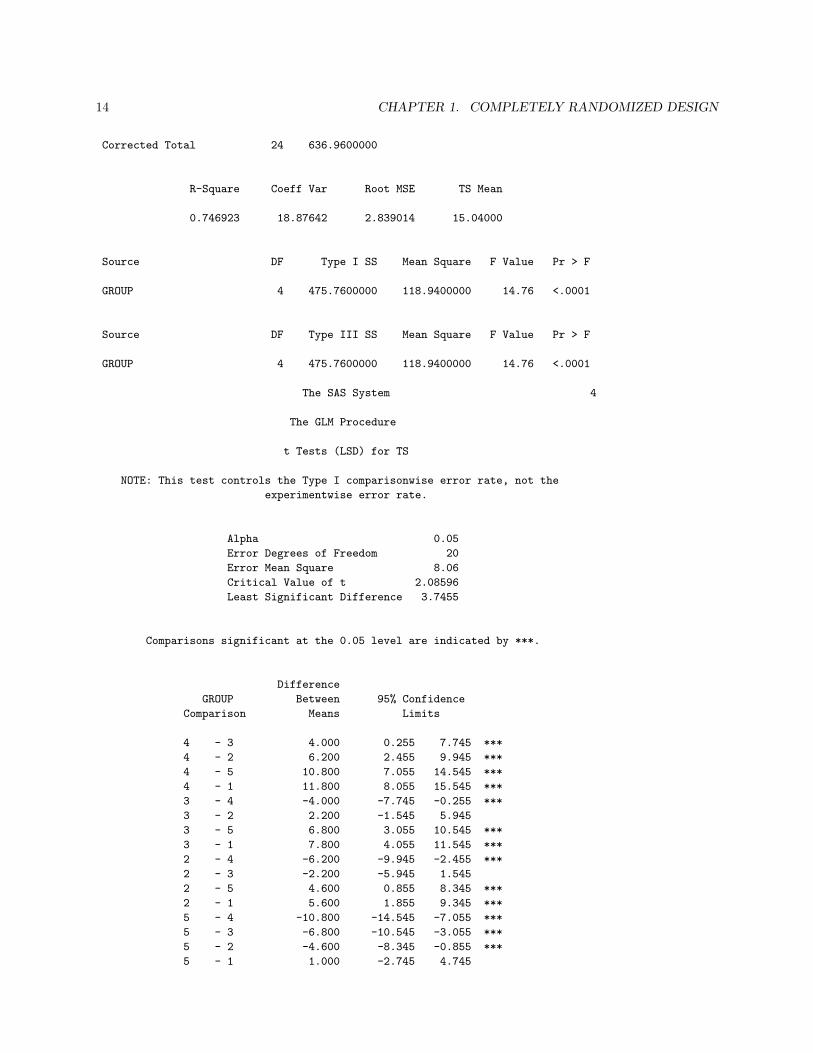
The tensile strength of a synthetic fiber used to make cloth for men’s shirts is of interest to a manufacturer.It is suspected that the strength is affected by the percentage of cotton in the fiber. Five levels of cottonpercentage are considered: 15%, 20%, 25%, 30% and 35%. For each percentage of cotton in the fiber,strength measurements (time to break when subject to a stress) are made on five pieces of fiber.
15 20 25 30 357 12 14 19 77 17 18 25 10
15 12 18 22 1111 18 19 19 159 18 19 23 11
The corresponding ANOVA table is
Source df SS MS F0
Between 4 475.76 118.94 F0 = 14.76Within (Error) 20 161.20 8.06Total 24 636.96
Performing the test at α = .01 one can easily conclude that the percentage of cotton has a significanteffect on fiber strength since F0 = 14.76 is greater than the tabulated F4,20(.01) = 4.43.
The estimate of the overall mean is µ = y.. = 15.04. Point estimates of the treatment effects are
τ1 = y1. − y.. = 9.80− 15.04 = −5.24τ2 = y2. − y.. = 15.40− 15.04 = 0.36τ3 = y3. − y.. = 17.60− 15.04 = −2.56τ4 = y4. − y.. = 21.60− 15.04 = 6.56τ5 = y5. − y.. = 10.80− 15.04 = −4.24
A 95% percent CI on the mean treatment 4 is
21.60± (2.086)√
8.06/5 ,
which gives the interval 18.95 ≤ µ4 ≤ 24.25.

1.2. THE FIXED EFFECTS MODEL 5
1.2.3 Comparison of Individual Treatment Means
Suppose we are interested in a certain linear combination of the treatment means, say,
L =k∑
i=1
liµi ,
where li, i = 1, · · · , k, are known real numbers not all zero.The natural estimate of L is
L =k∑
i=1
liµi =k∑
i=1
liyi. .
Under the one-way classification model (1.1), we have :
1. L follows a N(L, σ2∑k
i=1 l2i /ni),
2. L−L√MSW (
Pki=1 l2i /ni)
follows a tn−k distribution,
3. L± tn−k(α/2)√
MSW (∑k
i=1 l2i /ni),
4. An α-level test of
H0 : L = 0HA : L 6= 0
is ∣∣∣∣∣L√
MSW (∑k
i=1 l2i /ni)
∣∣∣∣∣ > tn−k(α/2) .
A linear combination of all the treatment means
φ =k∑
i=1
ciµi
is known as a contrast of µ1, · · · , µk if∑k
i=1 ci = 0. Its sample estimate is
φ =k∑
i=1
ciyi. .
Examples of contrasts are µ1 − µ2 and µ1 − µ.Consider r contrasts of µ1, · · · , µk, called planned comparisons, such as,
φi =k∑
s=1
cisµs withk∑
s=1
cis = 0 for i = 1, · · · , r ,
and the experiment consists ofH0 : φ1 = 0 · · · H0 : φr = 0
HA : φ1 6= 0 · · · HA : φr 6= 0

6 CHAPTER 1. COMPLETELY RANDOMIZED DESIGN
Example
The most common example is the set of all(k2
)pairwise tests
H0 : µi = µj
HA : µi 6= µj
for 1 ≤ i < j ≤ k of all µ1, · · · , µk. The experiment consists of all(k2
)pairwise tests. An experimentwise
error occurs if at least one of the null hypotheses is declared significant when H0 : µ1 = · · · = µk is knownto be true.
The Least Significant Difference (LSD) Method
Suppose that following an ANOVA F test where the null hypothesis is rejected, we wish to test H0 : µi = µj ,for all i 6= j. This could be done using the t statistic
t0 =yi. − yj.√
MSW (1/ni + 1/nj)
and comparing it to tn−k(α/2). An equivalent test declares µi and µj to be significantly different if |yi.−yj.| >LSD, where
LSD = tn−k(α/2)√
MSW (1/ni + 1/nj) .
The following gives a summary of the steps.
Stage 1 : Test H0 : µ1 = · · · = µk with F0 = MSB/MSW .
• if F0 < Fk−1,n−k(α), then declare H0 : µ1 = · · · = µk true and stop.
• if F0 > Fk−1,n−k(α), then go to Stage 2.
Stage 2 : Test
H0 : µi = µj
HA : µi 6= µj
for all(k2
)pairs with
|tij | = |yi. − yj.|√MSW (1/ni + 1/nj)
• if |tij | < tn−k(α/2), then accept H0 : µi = µj .
• if |tij | > tn−k(α/2), then reject H0 : µi = µj .
Example
Consider the fabric strength example we considered above. The ANOVA F -test rejected H0 : µ1 = · · · = µ5.The LSD at α = .05 is
LSD = t20(.025)√
MSW (1/5 + 1/5) = 2.086
√2(8.06)
5= 3.75 .
Thus any pair of treatment averages that differ by more than 3.75 would imply that the corresponding pair ofpopulation means are significantly different. The
(52
)= 10 pairwise differences among the treatment means
are

1.2. THE FIXED EFFECTS MODEL 7
y1. − y2. = 9.8− 15.4 = −5.6∗
y1. − y3. = 9.8− 17.6 = −7.8∗
y1. − y4. = 9.8− 21.6 = −11.8∗
y1. − y5. = 9.8− 10.8 = −1.0y2. − y3. = 15.4− 17.6 = −2.2y2. − y4. = 15.4− 21.6 = −6.2∗
y2. − y5. = 15.4− 10.8 = 4.6∗
y3. − y4. = 17.6− 21.6 = −4.0∗
y3. − y5. = 17.6− 10.8 = 6.8∗
y4. − y5. = 21.6− 10.8 = 10.8∗
Using underlining the result may be summarized as
y1. y5. y2. y3. y4.
9.8 10.8 15.4 17.6 21.6
As k gets large the experimentwise error becomes large. Sometimes we also find that the LSD fails tofind any significant pairwise differences while the F -test declares significance. This is due to the fact thatthe ANOVA F -test considers all possible comparisons, not just pairwise comparisons.
Scheffe’s Method for Comparing all Contrasts
Often we are interested in comparing different combinations of the treatment means. Scheffe (1953) hasproposed a method for comparing all possible contrasts between treatment means. The Scheffe methodcontrols the experimentwise error rate at level α.
Consider the r contrasts
φi =k∑
s=1
cisµs withk∑
s=1
cis = 0 for i = 1, · · · , r ,
and the experiment consists ofH0 : φ1 = 0 · · · H0 : φr = 0
HA : φ1 6= 0 · · · HA : φr 6= 0
The Scheffe method declares φi to be significant if
|φi| > Sα,i ,
where
φi =k∑
s=1
cisys.
and
Sα,i =√
(k − 1)Fk−1,n−k(α)
√√√√MSW
k∑s=1
(c2is/ni) .
Example
As an example, consider the fabric strength data and suppose that we are interested in the contrasts
φ1 = µ1 + µ3 − µ4 − µ5
andφ2 = µ1 − µ4 .

8 CHAPTER 1. COMPLETELY RANDOMIZED DESIGN
The sample estimates of these contrasts are
φ1 = y1. + y3. − y4. − y5. = 5.00
andφ2 = y1. − y4. = −11.80 .
We compute the Scheffe 1% critical values as
S.01,1 =√
(k − 1)Fk−1,n−k(.01)
√√√√MSW
k∑s=1
(c21s/n1)
=√
4(4.43)√
8.06(1 + 1 + 1 + 1)/5= 10.69
and
S.01,2 =√
(k − 1)Fk−1,n−k(.01)
√√√√MSW
k∑s=1
(c22s/n2)
=√
4(4.43)√
8.06(1 + 1)/5= 7.58
Since |φ1| < S.01,1, we conclude that the contrast φ1 = µ1 + µ3 − µ4 − µ5 is not significantly differentfrom zero. However, since |φ2| > S.01,2, we conclude that φ2 = µ1 − µ2 is significantly different from zero;that is, the mean strengths of treatments 1 and 4 differ significantly.
The Tukey-Kramer Method
The Tukey-Kramer procedure declares two means, µi and µj , to be significantly different if the absolutevalue of their sample differences exceeds
Tα = qk,n−k(α)
√MSW
2
( 1ni
+1nj
),
where qk,n−k(α) is the α percentile value of the studentized range distribution with k groups and n − kdegrees of freedom.
Example
Reconsider the fabric strength example. From the studentized range distribution table, we find thatq4,20(.05) = 4.23. Thus, a pair of means, µi and µj , would be declared significantly different if |yi. − yj.|exceeds
T.05 = 4.23
√8.062
(15
+15
)= 5.37 .
Using this value, we find that the following pairs of means do not significantly differ:
µ1 and µ5
µ5 and µ2
µ2 and µ3
µ3 and µ4
Notice that this result differs from the one reported by the LSD method.

1.2. THE FIXED EFFECTS MODEL 9
The Bonferroni Procedure
We start with the Bonferroni Inequality. Let A1, A2, · · · , Ak be k arbitrary events with P (Ai) ≥ 1 − α/k.Then P (A1 ∩A2 ∩ · · · ∩Ak) ≥ 1− α.
The proof of this result is left as an exercise.We may use this inequality to make simultaneous inference about linear combinations of treatment means
in a one-way fixed effects ANOVA set up.Let L1, L2, · · · , Lr be r linear combinations of µ1, · · · , µk where Li =
∑kj=1 lijµj and Li =
∑kj=1 lij yj.
for i = 1, · · · , r.A (1− α)100% simultaneous confidence interval for L1, · · · , Lr is
Li ± tn−k
( α
2r
)√√√√MSW
k∑
j=1
l2ij/nj .
for i = 1, · · · , r.A Bonferroni α-level test of
H0 : µ1 = µ2 = · · · = µk
is performed by testingH0 : µi = µj vs. HA : µi 6= µj
with
tij|yi. − yj.|√
MSW (1/ni + 1/nj)> tn−k
(α
2(k2
))
,
for 1 ≤ i < j ≤ k.There is no need to perform an overall F -test.
Example
Consider the tensile strength example considered above. We wish to test
H0 : µ1 = · · · = µ5
at .05 level of significance. This is done using
t20(.05/(2 ∗ 10)) = t20(.0025) = 3.153 .
So the test rejects H0 : µi = µj in favor of HA : µi 6= µj if |yi. − yj.| exceeds
3.153√
MSW (2/5) = 5.66 .
Exercise : Use underlining to summarize the results of the Bonferroni testing procedure.
Dunnett’s Method for Comparing Treatments to a Control
Assume µ1 is a control mean and µ2, · · · , µk are k − 1 treatment means. Our purpose here is to find a setof (1− α)100% simultaneous confidence intervals for the k − 1 pairwise differences comparing treatment tocontrol, µi − µ1, for i = 2, · · · , k.
Dunnett’s method rejects the null hypothesis H0 : µi = µ1 at level α if
|yi. − y1.| > dk−1,n−k(α)√
MSW (1/ni + 1/n1) ,
for i = 2, · · · , k.The value dk−1,n−k(α) is read from a table.

10 CHAPTER 1. COMPLETELY RANDOMIZED DESIGN
Example
Consider the tensile strength example above and let treatment 5 be the control. The Dunnett critical valueis d4,20(.05) = 2.65. Thus the critical difference is
d4,20(.05)√
MSW (2/5) = 4.76
So the test rejects H0 : µi = µ5 if|yi. − y5.| > 4.76 .
Only the differences y3. − y5. = 6.8 and y4. − y5. = 10.8 indicate any significant difference. Thus weconclude µ3 6= µ5 and µ4 6= µ5.
1.3 The Random Effects Model
The treatments in an experiment may be a random sample from a larger population of treatments. Ourpurpose is to estimate (and test, if any) the variability among the treatments in the population. Such amodel is known as a random effects model. The mathematical representation of the model is the same asthe fixed effects model:
yij = µ + τi + εij , i = 1, · · · , k, j = 1, · · · , ni ,
except for the assumptions underlying the model.
Assumptions
1. The treatment effects, τi, are a random sample from a population that is normally distributed withmean 0 and variance σ2
τ , i.e. τi ∼ N(0, σ2τ ).
2. The εij are random errors which follow the normal distribution with mean 0 and common variance σ2.
If the τi are independent of εij , the variance of an observation will be
Var(yij) = σ2 + σ2τ .
The two variances, σ2 and σ2τ are known as variance components.
The usual partition of the total sum of squares still holds:
SST = SSB + SSW .
Since we are interested in the bigger population of treatments, the hypothesis of interest is
H0 : σ2τ = 0
versusHA : σ2
τ > 0 .
If the hypothesis H0 : σ2τ = 0 is rejected in favor of HA : σ2
τ > 0, then we claim that there is a significantdifference among all the treatments.
Testing is performed using the same F statistic that we used for the fixed effects model:
F0 =MSB
MSW
An α-level test rejects H0 if F0 > Fk−1,n−k(α).
The estimators of the variance components are
σ2 = MSW

1.3. THE RANDOM EFFECTS MODEL 11
andσ2
τ =MSB −MSW
n0,
where
n0 =1
k − 1
[k∑
i=1
ni −∑k
i=1 n2i∑k
i=1 ni
].
We are usually interested in the proportion of the variance of an observation, Var(yij), that is the resultof the differences among the treatments:
σ2τ
σ2 + σ2τ
.
A 100(1− α)% confidence interval for σ2τ/(σ2 + σ2
τ ) is(
L
1 + L,
U
1 + U
),
where
L =1n0
(MSB
MSW
1Fk−1,n−k(α/2)
− 1
),
and
U =1n0
(MSB
MSW
1Fk−1,n−k(1− α/2)
− 1
).
The following example is taken from from Montgomery : Design and Analysis of Experiments.
Example
A textile company weaves a fabric on a large number of looms. They would like the looms to be homogeneousso that they obtain a fabric of uniform strength. The process engineer suspects that, in addition to the usualvariation in strength within samples of fabric from the same loom, there may also be significant variationsin strength between looms. To investigate this, he selects four looms at random and makes four strengthdeterminations on the fabric manufactured on each loom. The data are given in the following table:
ObservationsLooms 1 2 3 4
1 98 97 99 962 91 90 93 923 96 95 97 954 95 96 99 98
The corresponding ANOVA table is
Source df SS MS F0
Between (Looms) 3 89.19 29.73 15.68Within (Error) 12 22.75 1.90Total 15 111.94
Since F0 > F3,12(.05), we conclude that the looms in the plant differ significantly.The variance components are estimated by
σ2 = 1.90
andσ2
τ =29.73− 1.90
4= 6.96 .

12 CHAPTER 1. COMPLETELY RANDOMIZED DESIGN
Thus, the variance of any observation on strength is estimated by σ2 + σ2τ = 8.86. Most of this variability
(about 6.96/8.86 = 79%) is attributable to the difference among looms. The engineer must now try to isolatethe causes for the difference in loom performance (faulty set-up, poorly trained operators, . . . ).
Lets now find a 95% confidence interval for σ2τ/(σ2 + σ2
τ ). From properties of the F distribution wehave that Fa,b(α) = 1/Fb,a(1 − α). From the F table we see that F3,12(.025) = 4.47 and F3,12(.975) =1/F12,3(.025) = 1/5.22 = 0.192. Thus
L =14
[(29.731.90
)(1
4.47
)− 1
]= 0.625
and
U =14
[(29.731.90
)(1
0.192
)− 1
]= 20.124
which gives the 95% confidence interval
(0.625/1.625 = 0.39 , 20.124/21.124 = 0.95) .
We conclude that the variability among looms accounts for between 39 and 95 percent of the variance in theobserved strength of fabric produced.
Using SAS
The following SAS code may be used to analyze the tensile strength example considered in the fixed effectsCRD case.
OPTIONS LS=80 PS=66 NODATE;
DATA MONT;
INPUT TS GROUP@@;
CARDS;
7 1 7 1 15 1 11 1 9 1
12 2 17 2 12 2 18 2 18 2
14 3 18 3 18 3 19 3 19 3
19 4 25 4 22 4 19 4 23 4
7 5 10 5 11 5 15 5 11 5
;
/* print the data */
PROC PRINT DATA=MONT;
RUN;
QUIT;
PROC GLM;
CLASS GROUP;
MODEL TS=GROUP;
MEANS GROUP/ CLDIFF BON TUKEY SCHEFFE LSD DUNNETT(’5’);
CONTRAST ’PHI1’ GROUP 1 0 1 -1 -1;
ESTIMATE ’PHI1’ GROUP 1 0 1 -1 -1;
CONTRAST ’PHI2’ GROUP 1 0 0 -1 0;
ESTIMATE ’PHI2’ GROUP 1 0 0 -1 0;
RUN;
QUIT;
A random effects model may be analyzed using the RANDOM statement to specify the random factor:PROC GLM DATA=A1;
CLASS OFFICER;MODEL RATING=OFFICER;RANDOM OFFICER;
RUN;

1.3. THE RANDOM EFFECTS MODEL 13
SAS Output
The SAS System 1
Obs TS GROUP
1 7 1
2 7 1
3 15 1
4 11 1
5 9 1
6 12 2
7 17 2
8 12 2
9 18 2
10 18 2
11 14 3
12 18 3
13 18 3
14 19 3
15 19 3
16 19 4
17 25 4
18 22 4
19 19 4
20 23 4
21 7 5
22 10 5
23 11 5
24 15 5
25 11 5
The SAS System 2
The GLM Procedure
Class Level Information
Class Levels Values
GROUP 5 1 2 3 4 5
Number of observations 25
The SAS System 3
The GLM Procedure
Dependent Variable: TS
Sum of
Source DF Squares Mean Square F Value Pr > F
Model 4 475.7600000 118.9400000 14.76 <.0001
Error 20 161.2000000 8.0600000
14 CHAPTER 1. COMPLETELY RANDOMIZED DESIGN
Corrected Total 24 636.9600000
R-Square Coeff Var Root MSE TS Mean
0.746923 18.87642 2.839014 15.04000
Source DF Type I SS Mean Square F Value Pr > F
GROUP 4 475.7600000 118.9400000 14.76 <.0001
Source DF Type III SS Mean Square F Value Pr > F
GROUP 4 475.7600000 118.9400000 14.76 <.0001
The SAS System 4
The GLM Procedure
t Tests (LSD) for TS
NOTE: This test controls the Type I comparisonwise error rate, not the
experimentwise error rate.
Alpha 0.05
Error Degrees of Freedom 20
Error Mean Square 8.06
Critical Value of t 2.08596
Least Significant Difference 3.7455
Comparisons significant at the 0.05 level are indicated by ***.
Difference
GROUP Between 95% Confidence
Comparison Means Limits
4 - 3 4.000 0.255 7.745 ***
4 - 2 6.200 2.455 9.945 ***
4 - 5 10.800 7.055 14.545 ***
4 - 1 11.800 8.055 15.545 ***
3 - 4 -4.000 -7.745 -0.255 ***
3 - 2 2.200 -1.545 5.945
3 - 5 6.800 3.055 10.545 ***
3 - 1 7.800 4.055 11.545 ***
2 - 4 -6.200 -9.945 -2.455 ***
2 - 3 -2.200 -5.945 1.545
2 - 5 4.600 0.855 8.345 ***
2 - 1 5.600 1.855 9.345 ***
5 - 4 -10.800 -14.545 -7.055 ***
5 - 3 -6.800 -10.545 -3.055 ***
5 - 2 -4.600 -8.345 -0.855 ***
5 - 1 1.000 -2.745 4.745

1.3. THE RANDOM EFFECTS MODEL 15
1 - 4 -11.800 -15.545 -8.055 ***
1 - 3 -7.800 -11.545 -4.055 ***
1 - 2 -5.600 -9.345 -1.855 ***
1 - 5 -1.000 -4.745 2.745
The SAS System 5
The GLM Procedure
Tukey’s Studentized Range (HSD) Test for TS
NOTE: This test controls the Type I experimentwise error rate.
Alpha 0.05
Error Degrees of Freedom 20
Error Mean Square 8.06
Critical Value of Studentized Range 4.23186
Minimum Significant Difference 5.373
Comparisons significant at the 0.05 level are indicated by ***.
Difference
GROUP Between Simultaneous 95%
Comparison Means Confidence Limits
4 - 3 4.000 -1.373 9.373
4 - 2 6.200 0.827 11.573 ***
4 - 5 10.800 5.427 16.173 ***
4 - 1 11.800 6.427 17.173 ***
3 - 4 -4.000 -9.373 1.373
3 - 2 2.200 -3.173 7.573
3 - 5 6.800 1.427 12.173 ***
3 - 1 7.800 2.427 13.173 ***
2 - 4 -6.200 -11.573 -0.827 ***
2 - 3 -2.200 -7.573 3.173
2 - 5 4.600 -0.773 9.973
2 - 1 5.600 0.227 10.973 ***
5 - 4 -10.800 -16.173 -5.427 ***
5 - 3 -6.800 -12.173 -1.427 ***
5 - 2 -4.600 -9.973 0.773
5 - 1 1.000 -4.373 6.373
1 - 4 -11.800 -17.173 -6.427 ***
1 - 3 -7.800 -13.173 -2.427 ***
1 - 2 -5.600 -10.973 -0.227 ***
1 - 5 -1.000 -6.373 4.373
The SAS System 6
The GLM Procedure
Bonferroni (Dunn) t Tests for TS
NOTE: This test controls the Type I experimentwise error rate, but
it generally

16 CHAPTER 1. COMPLETELY RANDOMIZED DESIGN
has a higher Type II error rate than Tukey’s for all pairwise comparisons.
Alpha 0.05
Error Degrees of Freedom 20
Error Mean Square 8.06
Critical Value of t 3.15340
Minimum Significant Difference 5.6621
Comparisons significant at the 0.05 level are indicated by ***.
Difference
GROUP Between Simultaneous 95%
Comparison Means Confidence Limits
4 - 3 4.000 -1.662 9.662
4 - 2 6.200 0.538 11.862 ***
4 - 5 10.800 5.138 16.462 ***
4 - 1 11.800 6.138 17.462 ***
3 - 4 -4.000 -9.662 1.662
3 - 2 2.200 -3.462 7.862
3 - 5 6.800 1.138 12.462 ***
3 - 1 7.800 2.138 13.462 ***
2 - 4 -6.200 -11.862 -0.538 ***
2 - 3 -2.200 -7.862 3.462
2 - 5 4.600 -1.062 10.262
2 - 1 5.600 -0.062 11.262
5 - 4 -10.800 -16.462 -5.138 ***
5 - 3 -6.800 -12.462 -1.138 ***
5 - 2 -4.600 -10.262 1.062
5 - 1 1.000 -4.662 6.662
1 - 4 -11.800 -17.462 -6.138 ***
1 - 3 -7.800 -13.462 -2.138 ***
1 - 2 -5.600 -11.262 0.062
1 - 5 -1.000 -6.662 4.662
The SAS System 7
The GLM Procedure
Scheffe’s Test for TS
NOTE: This test controls the Type I experimentwise error rate, but
it generally
has a higher Type II error rate than Tukey’s for all pairwise comparisons.
Alpha 0.05
Error Degrees of Freedom 20
Error Mean Square 8.06
Critical Value of F 2.86608
Minimum Significant Difference 6.0796
Comparisons significant at the 0.05 level are indicated by ***.

1.3. THE RANDOM EFFECTS MODEL 17
Difference
GROUP Between Simultaneous 95%
Comparison Means Confidence Limits
4 - 3 4.000 -2.080 10.080
4 - 2 6.200 0.120 12.280 ***
4 - 5 10.800 4.720 16.880 ***
4 - 1 11.800 5.720 17.880 ***
3 - 4 -4.000 -10.080 2.080
3 - 2 2.200 -3.880 8.280
3 - 5 6.800 0.720 12.880 ***
3 - 1 7.800 1.720 13.880 ***
2 - 4 -6.200 -12.280 -0.120 ***
2 - 3 -2.200 -8.280 3.880
2 - 5 4.600 -1.480 10.680
2 - 1 5.600 -0.480 11.680
5 - 4 -10.800 -16.880 -4.720 ***
5 - 3 -6.800 -12.880 -0.720 ***
5 - 2 -4.600 -10.680 1.480
5 - 1 1.000 -5.080 7.080
1 - 4 -11.800 -17.880 -5.720 ***
1 - 3 -7.800 -13.880 -1.720 ***
1 - 2 -5.600 -11.680 0.480
1 - 5 -1.000 -7.080 5.080
The SAS System 8
The GLM Procedure
Dunnett’s t Tests for TS
NOTE: This test controls the Type I experimentwise error for
comparisons of all
treatments against a control.
Alpha 0.05
Error Degrees of Freedom 20
Error Mean Square 8.06
Critical Value of Dunnett’s t 2.65112
Minimum Significant Difference 4.7602
Comparisons significant at the 0.05 level are indicated by ***.
Difference
GROUP Between Simultaneous 95%
Comparison Means Confidence Limits
4 - 5 10.800 6.040 15.560 ***
3 - 5 6.800 2.040 11.560 ***
2 - 5 4.600 -0.160 9.360
1 - 5 -1.000 -5.760 3.760

18 CHAPTER 1. COMPLETELY RANDOMIZED DESIGN
The SAS System 9
The GLM Procedure
Dependent Variable: TS
Contrast DF Contrast SS Mean Square F Value Pr > F
PHI1 1 31.2500000 31.2500000 3.88 0.0630
PHI2 1 348.1000000 348.1000000 43.19 <.0001
Standard
Parameter Estimate Error t Value Pr > |t|
PHI1 -5.0000000 2.53929124 -1.97 0.0630
PHI2 -11.8000000 1.79555005 -6.57 <.0001
1.4 More About the One-Way Model
1.4.1 Model Adequacy Checking
Consider the one-way CRD model
yij = µ + τi + εij , i = 1, · · · , k, j = 1, · · · , ni ,
where it is assumed that εij ∼i.i.d. N(0, σ2). In the random effects model, we additionally assume thatτi ∼i.i.d. N(0, σ2
τ ) independently of εij .Diagnostics depend on the residuals,
eij = yij − yij = yij − yi.
The Normality Assumption
The simplest check for normality involves plotting the empirical quantiles of the residuals against the expectedquantiles if the residuals were to follow a normal distribution. This is known as the normal QQ-plot. Otherformal tests for normality (Kolmogorov-Smirnov, Shapiro-Wilk, Anderson-Darling, Cramer-von Mises) mayalso be performed to assess the normality of the residuals.
Example
The following SAS code and partial output checks the normality assumption for the tensile strength exampleconsidered earlier. The results from the QQ-plot as well as the formal tests (α = .05) indicate that theresiduals are fairly normal.
SAS Code
OPTIONS LS=80 PS=66 NODATE; DATA MONT; INPUT TS GROUP@@; CARDS; 7
1 7 1 15 1 11 1 9 1 12 2 17 2 12 2 18 2 18 2 14 3 18 3 18 3 19 3
19 3 19 4 25 4 22 4 19 4 23 4 7 5 10 5 11 5 15 5 11 5 ;
TITLE1 ’STRENGTH VS. PERCENTAGE’; SYMBOL1 V=CIRCLE I=NONE;
PROC GPLOT DATA=MONT; PLOT TS*GROUP/FRAME; RUN; QUIT;

1.4. MORE ABOUT THE ONE-WAY MODEL 19
PROC GLM;
CLASS GROUP;
MODEL TS=GROUP;
OUTPUT OUT=DIAG R=RES P=PRED;
RUN;
QUIT;
PROC SORT DATA=DIAG;
BY PRED;
RUN;
QUIT;
TITLE1 ’RESIDUAL PLOT’;
SYMBOL1 V=CIRCLE I=SM50;
PROC GPLOT DATA=DIAG;
PLOT RES*PRED/FRAME;
RUN;
QUIT;
PROC UNIVARIATE DATA=DIAG NORMAL;
VAR RES;
TITLE1 ’QQ-PLOT OF RESIDUALS’;
QQPLOT RES/NORMAL (L=1 MU=EST SIGMA=EST);
RUN;
QUIT;
Partial Output
The UNIVARIATE Procedure
Variable: RES
Moments
N 25 Sum Weights 25
Mean 0 Sum Observations 0
Std Deviation 2.59165327 Variance 6.71666667
Skewness 0.11239681 Kurtosis -0.8683604
Uncorrected SS 161.2 Corrected SS 161.2
Coeff Variation . Std Error Mean 0.51833065
Basic Statistical Measures
Location Variability
Mean 0.00000 Std Deviation 2.59165
Median 0.40000 Variance 6.71667
Mode -3.40000 Range 9.00000
Interquartile Range 4.00000
NOTE: The mode displayed is the smallest of 7 modes with a count of 2.

20 CHAPTER 1. COMPLETELY RANDOMIZED DESIGN
Tests for Location: Mu0=0
Test -Statistic- -----p Value------
Student’s t t 0 Pr > |t| 1.0000
Sign M 2.5 Pr >= |M| 0.4244
Signed Rank S 0.5 Pr >= |S| 0.9896
Tests for Normality
Test --Statistic--- -----p Value------
Shapiro-Wilk W 0.943868 Pr < W 0.1818
Kolmogorov-Smirnov D 0.162123 Pr > D 0.0885
Cramer-von Mises W-Sq 0.080455 Pr > W-Sq 0.2026
Anderson-Darling A-Sq 0.518572 Pr > A-Sq 0.1775

1.4. MORE ABOUT THE ONE-WAY MODEL 21
Constant Variance Assumption
Once again there are graphical and formal tests for checking the constant variance assumption. The graphicaltool we shall utilize in this class is the plot of residuals versus predicted values. The hypothesis of interest is
H0 : σ21 = σ2
2 = · · · = σ2k
versusHA : σ2
i 6= σ2j for at least one pair i 6= j .
One procedure for testing the above hypothesis is Bartlett’s test. The test statistic is
B0 = 2.3026q
c
where
q = (n− k) log10 MSW −k∑
i=1
(ni − 1) log10 S2i

22 CHAPTER 1. COMPLETELY RANDOMIZED DESIGN
c = 1 +1
3(k − 1)
(k∑
i=1
( 1ni − 1
)− 1
n− k
)
We reject H0 if
B0 > χ2k−1(α)
where χ2k−1(α) is read from the chi-square table.
Bartlett’s test is too sensitive deviations from normality. So, it should not be used if the normalityassumption is not satisfied.
A test which is more robust to deviations from normality is Levene’s test. Levene’s test proceeds bycomputing
dij = |yij −mi| ,
where mi is the median of the observations in group i, and then running the usual ANOVA F -test using thetransformed observations, dij , instead of the original observations, yij .
Example
Once again we consider the tensile strength example. The plot of residuals versus predicted values (seeabove) indicates no serious departure from the constant variance assumption. The following modification tothe proc GLM code given above generates both Bartlett’s and Levene’s tests. The tests provide no evidencethat indicates the failure of the constant variance assumption.
Partial SAS Code
PROC GLM;
CLASS GROUP;
MODEL TS=GROUP;
MEANS GROUP/HOVTEST=BARTLETT HOVTEST=LEVENE;
RUN;
QUIT;
Partial SAS Output
The GLM Procedure
Levene’s Test for Homogeneity of TS Variance
ANOVA of Squared Deviations from Group Means
Sum of Mean
Source DF Squares Square F Value Pr > F
GROUP 4 91.6224 22.9056 0.45 0.7704
Error 20 1015.4 50.7720
Bartlett’s Test for Homogeneity of TS Variance
Source DF Chi-Square Pr > ChiSq
GROUP 4 0.9331 0.9198

1.4. MORE ABOUT THE ONE-WAY MODEL 23
1.4.2 Some Remedial Measures
The Kruskal-Wallis Test
When the assumption of normality is suspect, we may wish to use nonparametric alternatives to the F -test.The Kruskal-Wallis test is one such procedure based on the rank transformation.
To perform the Kruskal-Wallis test, we first rank all the observations, yij , in increasing order. Say theranks are Rij . The Kruskal-Wallis test statistic is
KW0 =1S2
[k∑
i=1
R2i.
ni− n(n + 1)2
4
]
where Ri. is the sum of the ranks of group i, and
S2 =1
n− 1
[k∑
i=1
ni∑
j=1
R2ij −
n(n + 1)2
4
]
The test rejects H0 : µ1 = · · · = µk if
KW0 > χ2k−1(α) .
Example
For the tensile strength data the ranks, Rij , of the observations are given in the following table:
15 20 25 30 352.0 9.0 11.0 20.5 2.02.0 14.0 16.5 25.0 5.0
12.5 9.5 16.5 23.0 7.07.0 16.5 20.5 20.5 12.54.0 16.5 20.5 24.0 7.0
Ri. 27.5 66.0 85.0 113.0 33.5
We find that S2 = 53.03 and KW0 = 19.25. From the chi-square table we get χ24(.01) = 13.28. Thus we
reject the null hypothesis and conclude that the treatments differ.The SAS procedure NPAR1WAY may be used to obtain the Kruskal-Wallis test.
OPTIONS LS=80 PS=66 NODATE;
DATA MONT;
INPUT TS GROUP@@;
CARDS;
7 1 7 1 15 1 11 1 9 1
12 2 17 2 12 2 18 2 18 2
14 3 18 3 18 3 19 3 19 3
19 4 25 4 22 4 19 4 23 4
7 5 10 5 11 5 15 5 11 5
;
PROC NPAR1WAY WILCOXON;
CLASS GROUP;
VAR TS;
RUN;
QUIT;

24 CHAPTER 1. COMPLETELY RANDOMIZED DESIGN
The NPAR1WAY Procedure
Wilcoxon Scores (Rank Sums) for Variable TS
Classified by Variable GROUP
Sum of Expected Std Dev Mean
GROUP N Scores Under H0 Under H0 Score
---------------------------------------------------------------------
1 5 27.50 65.0 14.634434 5.50
2 5 66.00 65.0 14.634434 13.20
3 5 85.00 65.0 14.634434 17.00
4 5 113.00 65.0 14.634434 22.60
5 5 33.50 65.0 14.634434 6.70
Average scores were used for ties.
Kruskal-Wallis Test
Chi-Square 19.0637
DF 4
Pr > Chi-Square 0.0008
Variance Stabilizing Transformations
There are several variance stabilizing transformations one might consider in the case of heterogeneity ofvariance (heteroscedasticity). The common transformations are
√y, log(y), 1/y, arcsin(
√y), 1/
√y .
A simple method of choosing the appropriate transformation is to plot log Si versus log yi. or regresslog Si versus log yi.. We then choose the transformation depending on the slope of the relationship. Thefollowing table may be used as a guide:
Slope Transformation0 No Transformation1/2 Square root1 Log3/2 Reciprocal square root2 Reciprocal
A slightly more involved technique of choosing a variance stabilizing transformation is the Box-Coxtransformation. It uses the maximum likelihood method to simultaneously estimate the transformationparameter as well as the overall mean and the treatment effects.

Chapter 2
Randomized Blocks, Latin Squares,and Related Designs
2.1 The Randomized Complete Block Design
2.1.1 Introduction
In a completely randomized design (CRD), treatments are assigned to the experimental units in a completelyrandom manner. The random error component arises because of all the variables which affect the dependentvariable except the one controlled variable, the treatment. Naturally, the experimenter wants to reduce theerrors which account for differences among observations within each treatment. One of the ways in whichthis could be achieved is through blocking. This is done by identifying supplemental variables that are usedto group experimental subjects that are homogeneous with respect to that variable. This creates differencesamong the blocks and makes observations within a block similar. The simplest design that would accomplishthis is known as a randomized complete block design (RCBD). Each block is divided into k subblocks of equalsize. Within each block the k treatments are assigned at random to the subblocks. The design is ”complete”in the sense that each block contains all the k treatments.
The following layout shows a RCBD with k treatments and b blocks. There is one observation pertreatment in each block and the treatments are run in a random order within each block.
Treatment 1 Treatment 2 · · · Treatment k
Block 1 y11 y21 · · · yk1
Block 2 y12 y22 · · · yk2
Block 3 y13 y23 · · · yk3
......
......
Block b y1b y2b · · · ykb
The statistical model for RCBD is
yij = µ + τi + βj + εij , i = 1, · · · , k, j = 1, · · · , b (2.1)
where
• µ is the overall mean,
• τi is the ith treatment effect,
• βj is the effect of the jth block, and
• εij is the random error term associated with the ijth observation.
25

26 CHAPTER 2. RANDOMIZED BLOCKS
We make the following assumptions concerning the RCBD model:
• ∑ki=1 τi = 0,
• ∑bj=1 βj = 0, and
• εij ∼i.i.d N(0, σ2).
We are mainly interested in testing the hypotheses
H0 : µ1 = µ2 = · · · = µk
HA : µi 6= µj for at least one pair i 6= j
Here the ith treatment mean is defined as
µi =1b
b∑
j=1
(µ + τi + βj) = µ + τi
Thus the above hypotheses may be written equivalently as
H0 : τ1 = τ2 = · · · = τk = 0HA : τi 6= 0 for at least one i
2.1.2 Decomposition of the Total Sum of Squares
Let n = kb be the total number of observations. Define
yi. =1b
b∑
j=1
yij , i = 1, · · · , k
y.j =1k
k∑
i=1
yij , j = 1, · · · , b
y.. =1n
k∑
i=1
b∑
j=1
yij =1k
k∑
i=1
yi. =1b
b∑
j=1
y.j
One may show that
k∑
i=1
b∑
j=1
(yij − y..)2 = b
k∑
i=1
(yi. − y..)2 + k
b∑
j=1
(y.j − y..)2
+k∑
i=1
b∑
j=1
(yij − yi. − y.j + y..)2
Thus the total sum of squares is partitioned into the sum of squares due to the treatments, the sum ofsquares due to the blocking, and the sum of squares due to error.
Symbolically,SST = SSTreatments + SSBlocks + SSE
The degrees of freedom are partitioned accordingly as
(n− 1) = (k − 1) + (b− 1) + (k − 1)(b− 1)

2.1. THE RANDOMIZED COMPLETE BLOCK DESIGN 27
2.1.3 Statistical Analysis
Testing
The test for equality of treatment means is done using the test statistic
F0 =MSTreatments
MSE
where
MSTreatments =SSTreatments
k − 1and MSE =
SSE
(k − 1)(b− 1).
An α level test rejects H0 ifF0 > Fk−1,(k−1)(b−1)(α) .
The ANOVA table for RCBD is
Source df SS MS F -statistic
Treatments k − 1 SSTreatments MSTreatments F0 =MSTreatments
MSE
Blocks b− 1 SSBlocks MSBlocks FB =MSBlocks
MSE
Error (k − 1)(b− 1) SSE MSE
Total n− 1 SST
Since there is no randomization of treatments across blocks the use of FB = MSBlocks/MSE as a testfor block effects is questionable. However, a large value of FB would indicate that the blocking variable isprobably having the intended effect of reducing noise.
Estimation
Estimation of the model parameters is performed using the least squares procedure as in the case of thecompletely randomized design. The estimators of µ, τi, and βj are obtained via minimization of the sum ofsquares of the errors
L =k∑
i=1
b∑
j=1
ε2ij =k∑
i=1
b∑
j=1
(yij − µ− τi − βj)2 .
The solution is
µ = y..
τi = yi. − y.. i = 1, · · · , k
βj = y.j − y.. j = 1, · · · , b
From the model in (2.1), we can see that the estimated values of yij are
yij = µ + τi + βj
= y.. + yi. − y.. + y.j − y..
= yi. + y.j − y..
Example
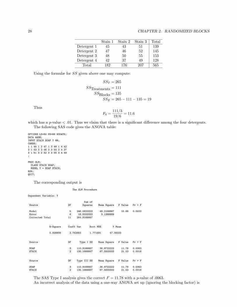
An experiment was designed to study the performance of four different detergents for cleaning clothes. Thefollowing ”cleanliness” readings (higher=cleaner) were obtained using a special device for three differenttypes of common stains. Is there a significant difference among the detergents?
28 CHAPTER 2. RANDOMIZED BLOCKS
Stain 1 Stain 2 Stain 3 TotalDetergent 1 45 43 51 139Detergent 2 47 46 52 145Detergent 3 48 50 55 153Detergent 4 42 37 49 128
Total 182 176 207 565
Using the formulæ for SS given above one may compute:
SST = 265SSTreatments = 111
SSBlocks = 135SSE = 265− 111− 135 = 19
Thus
F0 =111/319/6
= 11.6
which has a p-value < .01. Thus we claim that there is a significant difference among the four detergents.The following SAS code gives the ANOVA table:
OPTIONS LS=80 PS=66 NODATE;DATA WASH;INPUT STAIN SOAP Y @@;CARDS;1 1 45 1 2 47 1 3 48 1 4 422 1 43 2 2 46 2 3 50 2 4 373 1 51 3 2 52 3 3 55 3 4 49;
PROC GLM;CLASS STAIN SOAP;MODEL Y = SOAP STAIN;
RUN;QUIT;
The corresponding output is
The GLM Procedure
Dependent Variable: Y
Sum ofSource DF Squares Mean Square F Value Pr > F
Model 5 246.0833333 49.2166667 15.68 0.0022Error 6 18.8333333 3.1388889Corrected Total 11 264.9166667
R-Square Coeff Var Root MSE Y Mean
0.928908 3.762883 1.771691 47.08333
Source DF Type I SS Mean Square F Value Pr > F
SOAP 3 110.9166667 36.9722222 11.78 0.0063STAIN 2 135.1666667 67.5833333 21.53 0.0018
Source DF Type III SS Mean Square F Value Pr > F
SOAP 3 110.9166667 36.9722222 11.78 0.0063STAIN 2 135.1666667 67.5833333 21.53 0.0018
The SAS Type I analysis gives the correct F = 11.78 with a p-value of .0063.An incorrect analysis of the data using a one-way ANOVA set up (ignoring the blocking factor) is

2.1. THE RANDOMIZED COMPLETE BLOCK DESIGN 29
PROC GLM;CLASS SOAP;MODEL Y = SOAP;
RUN;QUIT;
The corresponding output is
The GLM Procedure
Dependent Variable: Y
Sum ofSource DF Squares Mean Square F Value Pr > F
Model 3 110.9166667 36.9722222 1.92 0.2048Error 8 154.0000000 19.2500000Corrected Total 11 264.9166667
Notice that H0 is not rejected indicating no significant difference among the detergents.
2.1.4 Relative Efficiency of the RCBD
The example in the previous section shows that RCBD and CRD may lead to different conclusions. Anatural question to ask is ”How much more efficient is the RCBD compared to a CRD?” One way to definethis relative efficiency is
R =(dfb + 1)(dfr + 3)(dfb + 3)(dfr + 1)
· σ2r
σ2b
where σ2r and σ2
b are the error variances of the CRD and RCBD, respectively, and dfr and dfb are thecorresponding error degrees of freedom. R is the increase in the number of replications required if a CRDto achieve the same precision as a RCBD.
Using the ANOVA table from RCBD, we may estimate σ2r and σ2
b as
σ2b = MSE
σ2r =
(b− 1)MSBlocks + b(k − 1)MSE
kb− 1
Example
Consider the detergent example considered in the previous section. From the ANOVA table for the RCBDwe see that
MSE = 3.139, dfb = (k − 1)(b− 1) = 6, dfr = kb− k = 8
Thus
σ2b = MSE = 3.139
σ2r =
(b− 1)MSBlocks + b(k − 1)MSE
kb− 1=
(2)(67.58) + (3)(3)(3.139)12− 1
= 14.86
The relative efficiency of RCBD to CRD is estimated to be
R =(dfb + 1)(dfr + 3)(dfb + 3)(dfr + 1)
· σ2r
σ2b
=(6 + 1)(8 + 3)(14.86)(6 + 3)(8 + 1)(3.139)
= 4.5
This means that a CRD will need about 4.5 as many replications to obtain the same precision as obtainedby blocking on stain types.
30 CHAPTER 2. RANDOMIZED BLOCKS
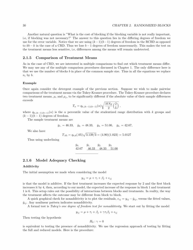
Another natural question is ”What is the cost of blocking if the blocking variable is not really important,i.e, if blocking was not necessary?” The answer to this question lies in the differing degrees of freedom weuse for the error variable. Notice that we are using (k−1)(b−1) degrees of freedom in the RCBD as opposedto kb− k in the case of a CRD. Thus we lose b− 1 degrees of freedom unnecessarily. This makes the test onthe treatment means less sensitive, i.e, differences among the means will remain undetected.
2.1.5 Comparison of Treatment Means
As in the case of CRD, we are interested in multiple comparisons to find out which treatment means differ.We may use any of the multiple comparison procedures discussed in Chapter 1. The only difference here isthat we use the number of blocks b in place of the common sample size. Thus in all the equations we replaceni by b.
Example
Once again consider the detergent example of the previous section. Suppose we wish to make pairwisecomparisons of the treatment means via the Tukey-Kramer procedure. The Tukey-Kramer procedure declarestwo treatment means, µi and µj , to be significantly different if the absolute value of their sample differencesexceeds
Tα = qk,(k−1)(b−1)(α)
√MSE
2
(2b
),
where qk,(k−1)(b−1)(α) is the α percentile value of the studentized range distribution with k groups and(k − 1)(b− 1) degrees of freedom.
The sample treatment means are
y1. = 46.33, y2. = 48.33, y3. = 51.00, y4. = 42.67,
We also haveT.05 = q4,6(.05)
√3.139/3 = (4.90)(1.023) = 5.0127
Thus using underlining
y4. y1. y2. y3.
42.67 46.33 48.33 51.00
2.1.6 Model Adequacy Checking
Additivity
The initial assumption we made when considering the model
yij = µ + τi + βj + εij
is that the model is additive. If the first treatment increases the expected response by 2 and the first blockincreases it by 4, then, according to our model, the expected increase of the response in block 1 and treatment1 is 6. This setup rules out the possibility of interactions between blocks and treatments. In reality, the waythe treatment affects the outcome may be different from block to block.
A quick graphical check for nonadditivity is to plot the residuals, eij = yij − yij , versus the fitted values,yij . Any nonlinear pattern indicates nonadditivity.
A formal test is Tukey’s one degree of freedom test for nonadditivity. We start out by fitting the model
yij = µ + τi + βj + γτiβj + εij
Then testing the hypothesisH0 : γ = 0
is equivalent to testing the presence of nonadditivity. We use the regression approach of testing by fittingthe full and reduced models. Here is the procedure:

2.1. THE RANDOMIZED COMPLETE BLOCK DESIGN 31
• Fit the modelyij = µ + τi + βj + εij
• Let eij and yij be the residual and the fitted value, respectively, corresponding to observation ij inresulting from fitting the model above.
• Let zij = y2ij and fit
zij = µ + τi + βj + εij
• Let rij = zij − zij be the residuals from this model.
• Regress eij on rij , i.e, fit the modeleij = α + γrij + εij
Let γ be the estimated slope.
• The sum of squares due to nonadditivity is
SSN = γ2k∑
i=1
b∑
j=1
r2ij
• The test statistic for nonadditivity is
F0 =SSN/1
(SSE − SSN )/[(k − 1)(b− 1)− 1]
Example
The impurity in a chemical product is believed to be affected by pressure. We will use temperature as ablocking variable. The data is given below.
PressureTemp 25 30 35 40 45100 5 4 6 3 5125 3 1 4 2 3150 1 1 3 1 2
The following SAS code is used.
Options ls=80 ps=66 nodate;
title "Tukey’s 1 DF Nonadditivity Test";
Data Chemical;
Input Temp @;
Do Pres = 25,30,35,40,45;
Input Im @;
output;
end;
cards;
100 5 4 6 3 5
125 3 1 4 2 3
150 1 1 3 1 2
;
proc print;
run;
quit;
proc glm;
class Temp Pres;
model Im = Temp Pres;

32 CHAPTER 2. RANDOMIZED BLOCKS
output out=out1 predicted=Pred;
run;
quit;
/* Form a new variable called Psquare. */
Data Tukey;
set out1;
Psquare = Pred*Pred;
run;
quit;
proc glm;
class Temp Pres;
model Im = Temp Pres Psquare;
run;
quit;
The following is the corresponding output.
Tukey’s 1 DF Nonadditivity Test
The GLM Procedure
Dependent Variable: Im
Sum ofSource DF Squares Mean Square F Value Pr > F
Model 7 35.03185550 5.00455079 18.42 0.0005
Error 7 1.90147783 0.27163969
Corrected Total 14 36.93333333
R-Square Coeff Var Root MSE Im Mean
0.948516 17.76786 0.521191 2.933333
Source DF Type I SS Mean Square F Value Pr > F
Temp 2 23.33333333 11.66666667 42.95 0.0001Pres 4 11.60000000 2.90000000 10.68 0.0042Psquare 1 0.09852217 0.09852217 0.36 0.5660
Source DF Type III SS Mean Square F Value Pr > F
Temp 2 1.25864083 0.62932041 2.32 0.1690Pres 4 1.09624963 0.27406241 1.01 0.4634Psquare 1 0.09852217 0.09852217 0.36 0.5660
Thus F0 = 0.36 with 1 and 7 degrees of freedom. It has a p-value of 0.5660. Thus we have no evidenceto declare nonadditivity.
Normality
The diagnostic tools for the normality of the error terms are the same as those use in the case of the CRD. Thegraphic tools are the QQ-plot and the histogram of the residuals. Formal tests like the Kolmogorov-Smirnovtest may also be used to assess the normality of the errors.
Example
Consider the detergent example above. The following SAS code gives the normality diagnostics.

2.1. THE RANDOMIZED COMPLETE BLOCK DESIGN 33
OPTIONS LS=80 PS=66 NODATE;
DATA WASH;
INPUT STAIN SOAP Y @@;
CARDS;
1 1 45 1 2 47 1 3 48 1 4 42
2 1 43 2 2 46 2 3 50 2 4 37
3 1 51 3 2 52 3 3 55 3 4 49
;
PROC GLM;
CLASS STAIN SOAP;
MODEL Y = SOAP STAIN;
MEANS SOAP/ TUKEY LINES;
OUTPUT OUT=DIAG R=RES P=PRED;
RUN;
QUIT;
PROC UNIVARIATE NOPRINT;
QQPLOT RES / NORMAL (L=1 MU=0 SIGMA=EST);
HIST RES / NORMAL (L=1 MU=0 SIGMA=EST);
RUN;
QUIT;
PROC GPLOT;
PLOT RES*SOAP;
PLOT RES*STAIN;
PLOT RES*PRED;
RUN;
QUIT;
The associated output is (figures given first):

34 CHAPTER 2. RANDOMIZED BLOCKS
Tukey’s Studentized Range (HSD) Test for Y
NOTE: This test controls the Type I experimentwise error rate, but it generallyhas a higher Type II error rate than REGWQ.
Alpha 0.05Error Degrees of Freedom 6Error Mean Square 3.138889Critical Value of Studentized Range 4.89559Minimum Significant Difference 5.0076
Means with the same letter are not significantly different.
TukeyGroupi
ng Mean N SOAP
A 51.000 3 3AA 48.333 3 2A
B A 46.333 3 1BB 42.667 3 4
RCBD Diagnostics
The UNIVARIATE ProcedureFitted Distribution for RES
Parameters for Normal Distribution
Parameter Symbol Estimate
Mean Mu 0Std Dev Sigma 1.252775
Goodness-of-Fit Tests for Normal Distribution
Test ---Statistic---- -----p Value-----
Cramer-von Mises W-Sq 0.01685612 Pr > W-Sq >0.250Anderson-Darling A-Sq 0.13386116 Pr > A-Sq >0.250
Th QQ-plot and the formal tests do not indicate the presence of nonnormality of the errors.

2.1. THE RANDOMIZED COMPLETE BLOCK DESIGN 35
Constant Variance
The tests for constant variance are the same as those used in the case of the CRD. One may use formaltests, such as Levene’s test or perform graphical checks to see if the assumption of constant variance issatisfied. The plots we need to examine in this case are residuals versus blocks, residuals versus treatments,and residuals versus predicted values.
The plots below (produced by the SAS code above) suggest that there may be nonconstant variance. Thespread of the residuals seems to differ from detergent to detergent. We may need to transform the valuesand rerun the analsis.

36 CHAPTER 2. RANDOMIZED BLOCKS
2.1.7 Missing Values
In a randomized complete block design, each treatment appears once in every block. A missing observationwould mean a loss of the completeness of the design. One way to proceed would be to use a multipleregression analysis. Another way would be to estimate the missing value.
If only one value is missing, say yij , then we substitute a value
y′ij =kTi. + bT.j − T..
(k − 1)(b− 1)
where
• Ti. is the total for treatment i,
• T.j is the total for block j, and
• T.. is the grand total.
We then substitute y′ij and carry out the ANOVA as usual. There will, however, be a loss of one degreeof freedom from both the total and error sums of squares. Since the substituted value adds no practicalinformation to the design, it should not be used in computations of means, for instance, when performingmultiple comparisons.
When more than one value is missing, they may be estimated via an iterative process. We first guessthe values of all except one. We then estimate the one missing value using the procedure above. We thenestimate the second one using the one estimated value and the remaining guessed values. We proceed toestimate the rest in a similar fashion. We repeat this process until convergence, i.e. difference betweenconsecutive estimates is small.
If several observations are missing from a single block or a single treatment group, we usually eliminatethe block or treatment in question. The analysis is then performed as if the block or treatment is nonexistent.
Example
Consider the detergent comparison example. Suppose y4,2 = 37 is missing. Note that the totals (without37) are T4. = 91, T.2 = 139, T.. = 528. The estimate is
y′4,2 =4(91) + 3(139)− 528
6= 42.17

2.1. THE RANDOMIZED COMPLETE BLOCK DESIGN 37
Now we just plug in this value and perform the analysis. We then need to modify the F value by handusing the correct degrees of freedom. The following SAS code will perform the RCBD ANOVA.
OPTIONS LS=80 PS=66 NODATE;
DATA WASH;
INPUT STAIN SOAP Y @@;
CARDS;
1 1 45 1 2 47 1 3 48 1 4 42
2 1 43 2 2 46 2 3 50 2 4 .
3 1 51 3 2 52 3 3 55 3 4 49
;
/* Replace the missing value with the estimated
value. */
DATA NEW;
SET WASH;
IF Y = . THEN Y = 42.17;
RUN;
QUIT;
PROC GLM;
CLASS STAIN SOAP;
MODEL Y = SOAP STAIN;
RUN;
QUIT;
The following is the associated SAS output.
The SAS System
The GLM Procedure
Dependent Variable: Y
Sum ofSource DF Squares Mean Square F Value Pr > F
Model 5 179.6703750 35.9340750 39.30 0.0002
Error 6 5.4861167 0.9143528
Corrected Total 11 185.1564917
R-Square Coeff Var Root MSE Y Mean
0.970370 2.012490 0.956218 47.51417
Source DF Type I SS Mean Square F Value Pr > F
SOAP 3 71.9305583 23.9768528 26.22 0.0008STAIN 2 107.7398167 53.8699083 58.92 0.0001
Source DF Type III SS Mean Square F Value Pr > F
SOAP 3 71.9305583 23.9768528 26.22 0.0008STAIN 2 107.7398167 53.8699083 58.92 0.0001
So, the correct F value is
F0 =71.93/35.49/5
= 21.84
which exceeds the tabulated value of F3,5(.05) = 5.41.

38 CHAPTER 2. RANDOMIZED BLOCKS
2.2 The Latin Square Design
The RCBD setup allows us to use only one factor as a blocking variable. However, sometimes we have twoor more factors that can be controlled.
Consider a situation where we have two blocking variables, row and column hereafter, and treatments.One design that handles such a case is the Latin square design. To build a Latin square design for ptreatments, we need p2 observations. These observations are then placed in a p× p grid made up of, p rowsand p columns, in such a way that each treatment occurs once, and only once, in each row and column.
Say we have 4 treatments, A,B,C, and D and two factors to control. A basic 4× 4 Latin square designis
ColumnRow 1 2 3 4
1 A B C D2 B C D A3 C D A B4 D A B C
The SAS procedure Proc PLAN may be used in association with Proc TABULATE to generatedesigns, in particular the Latin square design. The following SAS code gives the above basic 4× 4 design.
OPTIONS LS=80 PS=66 NODATE;TITLE ’A 4 BY 4 LATIN SQUARE DESIGN’;
PROC PLAN SEED=12345;FACTORS ROWS=4 ORDERED COLS=4 ORDERED /NOPRINT;TREATMENTS TMTS=4 CYCLIC;OUTPUT OUT=LAT44
ROWS NVALS=(1 2 3 4)COLS NVALS=(1 2 3 4)TMTS NVALS=(1 2 3 4);
RUN;QUIT;
PROC TABULATE;CLASS ROWS COLS;VAR TMTS;TABLE ROWS, COLS*TMTS;
RUN;QUIT;
-------------------------------------------------------
A 4 BY 4 LATIN SQUARE DESIGN
______________________________________| | COLS || |___________________|| | 1 | 2 | 3 | 4 || |____|____|____|____|| |TMTS|TMTS|TMTS|TMTS|| |____|____|____|____|| |Sum |Sum |Sum |Sum ||__________________|____|____|____|____||ROWS | | | | ||__________________| | | | ||1 | 1| 2| 3| 4||__________________|____|____|____|____||2 | 2| 3| 4| 1||__________________|____|____|____|____||3 | 3| 4| 1| 2||__________________|____|____|____|____||4 | 4| 1| 2| 3||__________________|____|____|____|____|

2.2. THE LATIN SQUARE DESIGN 39
The statistical model for a Latin square design is
yijk = µ + αi + τj + βk + εijk
i = 1, · · · , p
j = 1, · · · , p
k = 1, · · · , p
where
• µ is the grand mean,
• αi is the ith block 1 (row) effect,
• τj is the jth treatment effect,
• βk is the kth block 2 (column) effect, and
• εijk ∼i.i.d. N(0, σ2).
There is no interaction between rows, columns, and treatments; the model is completely additive.
2.2.1 Statistical Analysis
The total sum of squares, SST , partitions into sums of squares due to columns, rows, treatments, and error.An intuitive way of identifying the components is (since all the cross products are zero)
yijk = y...+ (yi.. − y...)+ (y.j. − y...)+ (y..k − y...)+ (yijk − yi.. − y.j. − y..k + 2y...)
= µ + αi + τj + βk + eijk
We haveSST = SSRow + SSTrt + SSCol + SSE
where
SST =∑∑ ∑
(yijk − y...)2
SSRow = p∑
(yi.. − y...)2
SSTrt = p∑
(y.j. − y...)2
SSCol = p∑
(y..k − y...)2
SSE =∑∑ ∑
(yijk − yi.. − y.j. − y..k + 2y...)2
Thus the ANOVA table for the Latin square design is
Source df SS MS F -statistic
Treatments p− 1 SSTrt MSTrt F0 = MST rtMSE
Rows p− 1 SSRow MSRow
Columns p− 1 SSCol MSCol
Error (p− 2)(p− 1) SSE MSE
Total p2 − 1 SST
The test statistic for testing for no differences in the treatment means is F0. An α level test rejects nullhypothesis if F0 > Fp−1,(p−2)(p−1)(α).
Multiple comparisons are performed in a similar manner as in the case of RCBD. The only difference isthat b is replaced by p and the error degrees of freedom becomes (p− 2)(p− 1) instead of (k − 1)(b− 1).

40 CHAPTER 2. RANDOMIZED BLOCKS
Example
Consider an experiment to investigate the effect of four different diets on milk production of cows. Thereare four cows in the study. During each lactation period the cows receive a different diet. Assume that thereis a washout period between diets so that previous diet does not affect future results. Lactation period andcows are used as blocking variables.
A 4× 4 Latin square design is implemented.
CowPeriod 1 2 3 4
1 A=38 B=39 C=45 D=412 B=32 C=37 D=38 A=303 C=35 D=36 A=37 B=324 D=33 A=30 B=35 C=33
The following gives the SAS analysis of the data.
OPTIONS LS=80 PS=66 NODATE;
DATA NEW;INPUT COW PERIOD DIET MILK @@;
CARDS;1 1 1 38 1 2 2 32 1 3 3 35 1 4 4 332 1 2 39 2 2 3 37 2 3 4 36 2 4 1 303 1 3 45 3 2 4 38 3 3 1 37 3 4 2 354 1 4 41 4 2 1 30 4 3 2 32 4 4 3 33
;RUN;QUIT;
PROC GLM;CLASS COW DIET PERIOD;MODEL MILK = DIET PERIOD COW;MEANS DIET/ LINES TUKEY;
RUN;QUIT;
-------------------------------------------------Dependent Variable: MILK
Sum ofSource DF Squares Mean Square F Value Pr > F
Model 9 242.5625000 26.9513889 33.17 0.0002
Error 6 4.8750000 0.8125000
Corrected Total 15 247.4375000
R-Square Coeff Var Root MSE MILK Mean
0.980298 2.525780 0.901388 35.68750
Source DF Type I SS Mean Square F Value Pr > F
DIET 3 40.6875000 13.5625000 16.69 0.0026PERIOD 3 147.1875000 49.0625000 60.38 <.0001COW 3 54.6875000 18.2291667 22.44 0.0012
Source DF Type III SS Mean Square F Value Pr > F
DIET 3 40.6875000 13.5625000 16.69 0.0026PERIOD 3 147.1875000 49.0625000 60.38 <.0001COW 3 54.6875000 18.2291667 22.44 0.0012
Tukey’s Studentized Range (HSD) Test for MILK
Alpha 0.05

2.2. THE LATIN SQUARE DESIGN 41
Error Degrees of Freedom 6Error Mean Square 0.8125Critical Value of Studentized Range 4.89559Minimum Significant Difference 2.2064
Means with the same letter are not significantly different.
Tukey Grouping Mean N DIET
A 37.5000 4 3AA 37.0000 4 4
B 34.5000 4 2BB 33.7500 4 1
Thus there diet has a significant effect (p-value=0.0026) on milk production. The Tukey-Kramer multiplecomparison procedure indicates that diets C and D do not differ significantly. The same result holds fordiets A and B. All other pairs are declared to be significantly different.
2.2.2 Missing Values
Missing values are estimated in a similar manner as in RCBD’s. If only yijk is missing, it is estimated by
y′ijk =p(Ti.. + T.j. + T..k)− 2T...
(p− 1)(p− 2)
where Ti.., T.j., T..k, and T... are the row i, treatment j, column k, and grand totals of the available observa-tions, respectively.
If more than one value is missing, we employ an iterative procedure similar to the one in RCBD.
2.2.3 Relative Efficiency
The relative efficiency of the Latin square design with respect to other designs is considered next.The estimated relative efficiency of a Latin square design with respect to a RCBD with the rows omitted
and the columns as blocks is
R(Latin, RCBDcol) =MSRow + (p− 1)MSE
pMSE
Similarly, the estimated relative efficiency of a Latin square design with respect to a RCBD with thecolumns omitted and the rows as blocks is
R(Latin, RCBDrow) =MSCol + (p− 1)MSE
pMSE
Furthermore, the estimated relative efficiency of a Latin square design with respect to a CRD
R(Latin, CRD) =MSRow + MSCol + (p− 1)MSE
(p + 1)MSE
For instance, considering the milk production example, we see that if we just use cows as blocks, we get
R(Latin, RCBDcows) =MSPeriod + (p− 1)MSE
pMSE=
49.06 + 3(.8125)4(.8125)
= 15.85
Thus a RCBD design with just cows as blocks would cost about 16 times as much as the present Latinsquare design to achieve the same sensitivity.

42 CHAPTER 2. RANDOMIZED BLOCKS
2.2.4 Replicated Latin Square
Replication of a Latin square is done by forming several Latin squares of the same dimension. This may bedone using
• same row and column blocks
• new rows and same columns
• same rows and new columns
• new rows and new columns
Examples
The following 3×3 Latin square designs are intended to illustrate the techniques of replicating Latin squares.
same rows; same columns :
1 2 3 replication1 A B C2 B C A 13 C A B
1 2 31 C B A2 B A C 23 A C B
1 2 31 B A C2 A C B 33 C B A
different rows; same columns :
1 2 3 replication1 A B C2 B C A 13 C A B
1 2 34 C B A5 B A C 26 A C B
1 2 37 B A C8 A C B 39 C B A
different rows; different columns :

2.2. THE LATIN SQUARE DESIGN 43
1 2 3 replication1 A B C2 B C A 13 C A B
4 5 64 C B A5 B A C 26 A C B
7 8 97 B A C8 A C B 39 C B A
Replication increases the error degrees of freedom without increasing the number of treatments. However,it adds a parameter (or parameters) in our model, thus increasing the complexity of the model.
The analysis of variance depends on the type of replication.
Replicated Square
This uses the same rows and columns and different randomization of the treatments within each square. Thestatistical model is
yijkl = µ + αi + τj + βk + ψl + εijkl
i = 1, · · · , p
j = 1, · · · , p
k = 1, · · · , p
l = 1, · · · , r
where r is the number of replications. Here ψl represents the effect of the lth replicate. The associatedANOVA table is
Source df SS MS F -statistic
Treatments p− 1 SSTrt MSTrt F0 = MST rtMSE
Rows p− 1 SSRow MSRow
Columns p− 1 SSCol MSCol
Replicate r − 1 SSRep MSRep
Error (p− 1)[r(p + 1)− 3] SSE MSE
Total rp2 − 1 SST
where
SST =∑∑ ∑∑
(yijkl − y....)2
SSTrt = np
p∑
j=1
(y.j.. − y....)2
SSRow = np
p∑
i=1
(yi... − y....)2
SSCol = np
p∑
k=1
(y..k. − y....)2
SSRep = p2r∑
l=1
(y...l − y....)2
and SSE is found by subtraction.
44 CHAPTER 2. RANDOMIZED BLOCKS
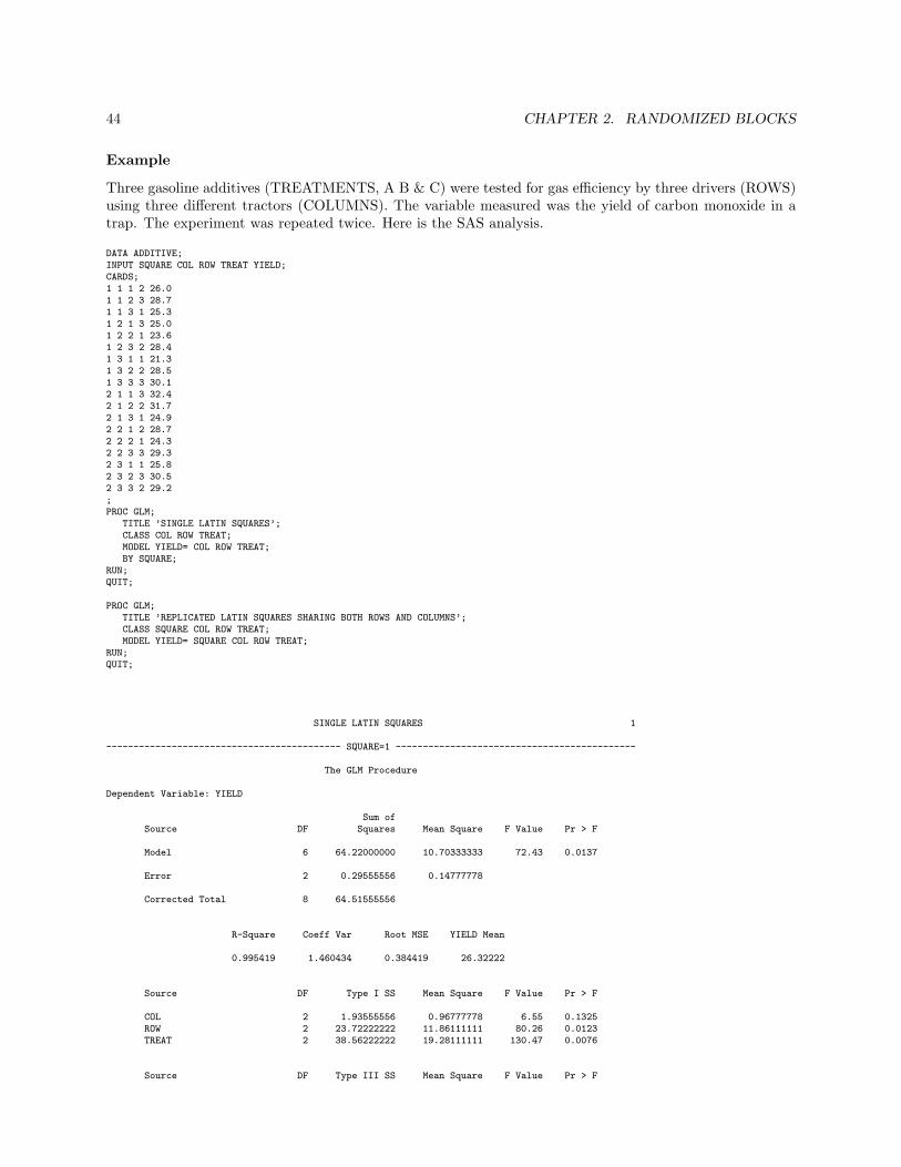
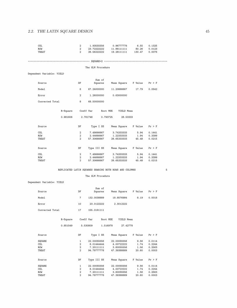
Example
Three gasoline additives (TREATMENTS, A B & C) were tested for gas efficiency by three drivers (ROWS)using three different tractors (COLUMNS). The variable measured was the yield of carbon monoxide in atrap. The experiment was repeated twice. Here is the SAS analysis.
DATA ADDITIVE;INPUT SQUARE COL ROW TREAT YIELD;CARDS;1 1 1 2 26.01 1 2 3 28.71 1 3 1 25.31 2 1 3 25.01 2 2 1 23.61 2 3 2 28.41 3 1 1 21.31 3 2 2 28.51 3 3 3 30.12 1 1 3 32.42 1 2 2 31.72 1 3 1 24.92 2 1 2 28.72 2 2 1 24.32 2 3 3 29.32 3 1 1 25.82 3 2 3 30.52 3 3 2 29.2;PROC GLM;
TITLE ’SINGLE LATIN SQUARES’;CLASS COL ROW TREAT;MODEL YIELD= COL ROW TREAT;BY SQUARE;
RUN;QUIT;
PROC GLM;TITLE ’REPLICATED LATIN SQUARES SHARING BOTH ROWS AND COLUMNS’;CLASS SQUARE COL ROW TREAT;MODEL YIELD= SQUARE COL ROW TREAT;
RUN;QUIT;
SINGLE LATIN SQUARES 1
------------------------------------------- SQUARE=1 --------------------------------------------
The GLM Procedure
Dependent Variable: YIELD
Sum ofSource DF Squares Mean Square F Value Pr > F
Model 6 64.22000000 10.70333333 72.43 0.0137
Error 2 0.29555556 0.14777778
Corrected Total 8 64.51555556
R-Square Coeff Var Root MSE YIELD Mean
0.995419 1.460434 0.384419 26.32222
Source DF Type I SS Mean Square F Value Pr > F
COL 2 1.93555556 0.96777778 6.55 0.1325ROW 2 23.72222222 11.86111111 80.26 0.0123TREAT 2 38.56222222 19.28111111 130.47 0.0076
Source DF Type III SS Mean Square F Value Pr > F
2.2. THE LATIN SQUARE DESIGN 45
COL 2 1.93555556 0.96777778 6.55 0.1325ROW 2 23.72222222 11.86111111 80.26 0.0123TREAT 2 38.56222222 19.28111111 130.47 0.0076
------------------------------------------- SQUARE=2 --------------------------------------------
The GLM Procedure
Dependent Variable: YIELD
Sum ofSource DF Squares Mean Square F Value Pr > F
Model 6 67.24000000 11.20666667 17.79 0.0542
Error 2 1.26000000 0.63000000
Corrected Total 8 68.50000000
R-Square Coeff Var Root MSE YIELD Mean
0.981606 2.781748 0.793725 28.53333
Source DF Type I SS Mean Square F Value Pr > F
COL 2 7.48666667 3.74333333 5.94 0.1441ROW 2 2.44666667 1.22333333 1.94 0.3399TREAT 2 57.30666667 28.65333333 45.48 0.0215
Source DF Type III SS Mean Square F Value Pr > F
COL 2 7.48666667 3.74333333 5.94 0.1441ROW 2 2.44666667 1.22333333 1.94 0.3399TREAT 2 57.30666667 28.65333333 45.48 0.0215
REPLICATED LATIN SQUARES SHARING BOTH ROWS AND COLUMNS 5
The GLM Procedure
Dependent Variable: YIELD
Sum ofSource DF Squares Mean Square F Value Pr > F
Model 7 132.0038889 18.8576984 8.19 0.0018
Error 10 23.0122222 2.3012222
Corrected Total 17 155.0161111
R-Square Coeff Var Root MSE YIELD Mean
0.851549 5.530809 1.516978 27.42778
Source DF Type I SS Mean Square F Value Pr > F
SQUARE 1 22.00055556 22.00055556 9.56 0.0114COL 2 8.01444444 4.00722222 1.74 0.2244ROW 2 7.20111111 3.60055556 1.56 0.2563TREAT 2 94.78777778 47.39388889 20.60 0.0003
Source DF Type III SS Mean Square F Value Pr > F
SQUARE 1 22.00055556 22.00055556 9.56 0.0114COL 2 8.01444444 4.00722222 1.74 0.2244ROW 2 7.20111111 3.60055556 1.56 0.2563TREAT 2 94.78777778 47.39388889 20.60 0.0003

46 CHAPTER 2. RANDOMIZED BLOCKS
Replicated Rows
In this instance the rows of different squares are independent but the columns are shared; i.e different rowsbut same columns. Thus, the treatment effect may be different for each square. The statistical model inshows this by nesting row effects within squares. The model is
yijkl = µ + αi(l) + τj + βk + ψl + εijkl
i = 1, · · · , p
j = 1, · · · , p
k = 1, · · · , p
l = 1, · · · , r
where αi(l) represents the effect of row i nested within replicate (square) l.The associated ANOVA table is
Source df SS MS F -statistic
Treatments p− 1 SSTrt MSTrt F0 = MST rtMSE
Rows r(p− 1) SSRow MSRow
Columns p− 1 SSCol MSCol
Replicate r − 1 SSRep MSRep
Error (p− 1)[rp− 2] SSE MSE
Total rp2 − 1 SST
Example
We will reanalyze the previous example; this time assuming we have six different drivers.
DATA ADDITIVE;INPUT SQUARE COL ROW TREAT YIELD;CARDS;1 1 1 2 26.01 1 2 3 28.71 1 3 1 25.31 2 1 3 25.01 2 2 1 23.61 2 3 2 28.41 3 1 1 21.31 3 2 2 28.51 3 3 3 30.12 1 4 3 32.42 1 5 2 31.72 1 6 1 24.92 2 4 2 28.72 2 5 1 24.32 2 6 3 29.32 3 4 1 25.82 3 5 3 30.52 3 6 2 29.2;
PROC GLM;TITLE ’REPLICATED LATIN SQUARES SHARING ONLY COLUMNS’;CLASS SQUARE COL ROW TREAT;MODEL YIELD= SQUARE COL ROW(SQUARE) TREAT;
RUN;QUIT;
REPLICATED LATIN SQUARES SHARING ONLY COLUMNS 7
The GLM Procedure
Dependent Variable: YIELD
Sum ofSource DF Squares Mean Square F Value Pr > F
Model 9 150.9716667 16.7746296 33.18 <.0001
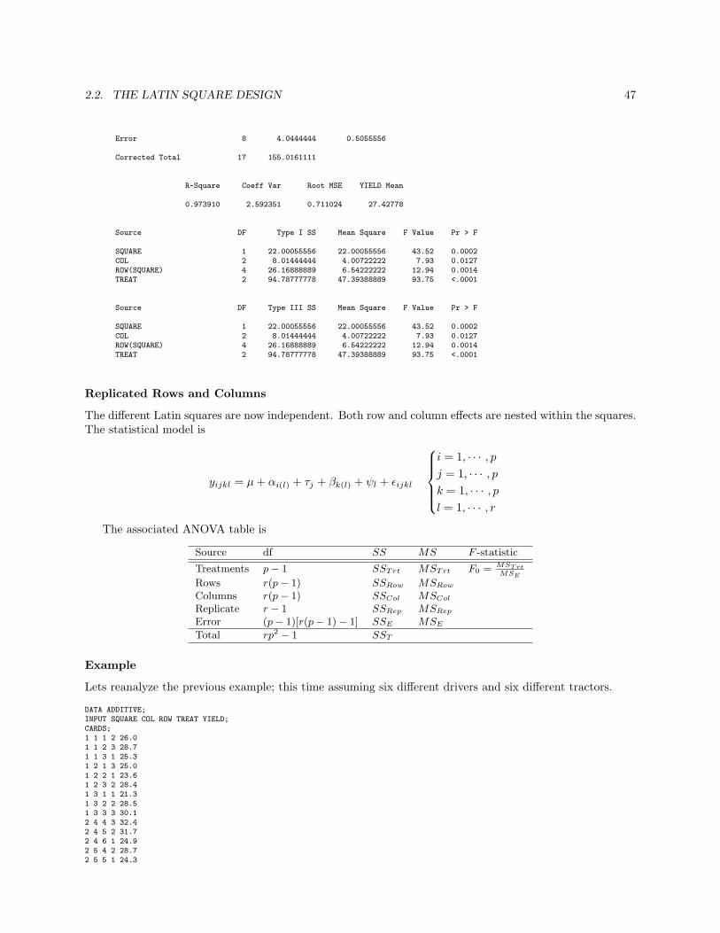
2.2. THE LATIN SQUARE DESIGN 47
Error 8 4.0444444 0.5055556
Corrected Total 17 155.0161111
R-Square Coeff Var Root MSE YIELD Mean
0.973910 2.592351 0.711024 27.42778
Source DF Type I SS Mean Square F Value Pr > F
SQUARE 1 22.00055556 22.00055556 43.52 0.0002COL 2 8.01444444 4.00722222 7.93 0.0127ROW(SQUARE) 4 26.16888889 6.54222222 12.94 0.0014TREAT 2 94.78777778 47.39388889 93.75 <.0001
Source DF Type III SS Mean Square F Value Pr > F
SQUARE 1 22.00055556 22.00055556 43.52 0.0002COL 2 8.01444444 4.00722222 7.93 0.0127ROW(SQUARE) 4 26.16888889 6.54222222 12.94 0.0014TREAT 2 94.78777778 47.39388889 93.75 <.0001
Replicated Rows and Columns
The different Latin squares are now independent. Both row and column effects are nested within the squares.The statistical model is
yijkl = µ + αi(l) + τj + βk(l) + ψl + εijkl
i = 1, · · · , p
j = 1, · · · , p
k = 1, · · · , p
l = 1, · · · , r
The associated ANOVA table is
Source df SS MS F -statistic
Treatments p− 1 SSTrt MSTrt F0 = MST rtMSE
Rows r(p− 1) SSRow MSRow
Columns r(p− 1) SSCol MSCol
Replicate r − 1 SSRep MSRep
Error (p− 1)[r(p− 1)− 1] SSE MSE
Total rp2 − 1 SST
Example
Lets reanalyze the previous example; this time assuming six different drivers and six different tractors.
DATA ADDITIVE;INPUT SQUARE COL ROW TREAT YIELD;CARDS;1 1 1 2 26.01 1 2 3 28.71 1 3 1 25.31 2 1 3 25.01 2 2 1 23.61 2 3 2 28.41 3 1 1 21.31 3 2 2 28.51 3 3 3 30.12 4 4 3 32.42 4 5 2 31.72 4 6 1 24.92 5 4 2 28.72 5 5 1 24.3
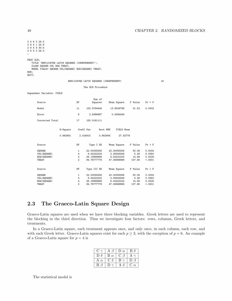
48 CHAPTER 2. RANDOMIZED BLOCKS
2 5 6 3 29.32 6 4 1 25.82 6 5 3 30.52 6 6 2 29.2;
PROC GLM;TITLE ’REPLICATED LATIN SQUARES (INDEPENDENT)’;CLASS SQUARE COL ROW TREAT;MODEL YIELD= SQUARE COL(SQUARE) ROW(SQUARE) TREAT;
RUN;QUIT;
REPLICATED LATIN SQUARES (INDEPENDENT) 16
The GLM Procedure
Dependent Variable: YIELD
Sum ofSource DF Squares Mean Square F Value Pr > F
Model 11 152.3794444 13.8526768 31.52 0.0002
Error 6 2.6366667 0.4394444
Corrected Total 17 155.0161111
R-Square Coeff Var Root MSE YIELD Mean
0.982991 2.416915 0.662906 27.42778
Source DF Type I SS Mean Square F Value Pr > F
SQUARE 1 22.00055556 22.00055556 50.06 0.0004COL(SQUARE) 4 9.42222222 2.35555556 5.36 0.0350ROW(SQUARE) 4 26.16888889 6.54222222 14.89 0.0029TREAT 2 94.78777778 47.39388889 107.85 <.0001
Source DF Type III SS Mean Square F Value Pr > F
SQUARE 1 22.00055556 22.00055556 50.06 0.0004COL(SQUARE) 4 9.42222222 2.35555556 5.36 0.0350ROW(SQUARE) 4 26.16888889 6.54222222 14.89 0.0029TREAT 2 94.78777778 47.39388889 107.85 <.0001
2.3 The Graeco-Latin Square Design
Graeco-Latin squares are used when we have three blocking variables. Greek letters are used to representthe blocking in the third direction. Thus we investigate four factors: rows, columns, Greek letters, andtreatments.
In a Graeco-Latin square, each treatment appears once, and only once, in each column, each row, andwith each Greek letter. Graeco-Latin squares exist for each p ≥ 3, with the exception of p = 6. An exampleof a Graeco-Latin square for p = 4 is
C γ A β D α B δD δ B α C β A γA α C δ B γ D βB β D γ A δ C α
The statistical model is

2.3. THE GRAECO-LATIN SQUARE DESIGN 49
yijkl = µ + αi + τj + βk + ψl + εijkl
i = 1, · · · , p
j = 1, · · · , p
k = 1, · · · , p
l = 1, · · · , p
where ψl is the effect of the lth Greek letter.The associated ANOVA table is
Source df SS MS F -statistic
Treatments p− 1 SSTrt MSTrt F0 = MST rtMSE
Greek letters p− 1 SSG MSG
Rows p− 1 SSRow MSRow
Columns p− 1 SSCol MSCol
Error (p− 1)(p− 3) SSE MSE
Total p2 − 1 SST
where
SST =∑∑ ∑∑
(yijkl − y....)2
SSTrt = p
p∑
j=1
(y.j.. − y....)2
SSRow = p
p∑
i=1
(yi... − y....)2
SSCol = p
p∑
k=1
(y..k. − y....)2
SSG = p
r∑
l=1
(y...l − y....)2
and SSE is found by subtraction.The following example is taken from Petersen : Design and Analysis of Experiments (1985).
Example
A food processor wanted to determine the effect of package design on the sale of one of his products. Hehad five designs to be tested : A,B, C,D, E. There were a number of sources of variation. These included:(1) day of the week, (2) differences among stores, and (3) effect of shelf height. He decided to conducta trial using a Graeco-Latin square design with five weekdays corresponding to the row classification, fivedifferent stores assigned to the column classification, and five shelf heights corresponding to the Greek letterclassification. The following table contains the results of his trial.
StoreDay 1 2 3 4 5Mon E α (238) C δ (228) B γ (158) D ε (188) A β (74)Tue D δ (149) B β (220) A α (92) C γ (169) E ε (282)Wed B ε (222) E γ (295) D β (104) A δ (54) C α (213)Thur C β (187) A ε (66) E δ (242) B α (122) D γ (90)Fri A γ (65) D α (118) C ε (279) E β (278) B γ (176)
The following is the SAS analysis.

50 CHAPTER 2. RANDOMIZED BLOCKS
OPTIONS LS=80 PS=66 NODATE;DATA GL;INPUT ROW COL TRT GREEK Y;CARDS;1 1 5 1 2381 2 3 4 2281 3 2 3 1581 4 4 5 1881 5 1 2 742 1 4 4 1492 2 2 2 2202 3 1 1 922 4 3 3 1692 5 5 5 2823 1 2 5 2223 2 5 3 2953 3 4 2 1043 4 1 4 543 5 3 1 2134 1 3 2 1874 2 1 5 664 3 5 4 2424 4 2 1 1224 5 4 3 905 1 1 3 655 2 4 1 1185 3 3 5 2795 4 5 2 2785 5 2 4 176;
PROC GLM;CLASS ROW COL TRT GREEK;MODEL Y = ROW COL TRT GREEK;
RUN;QUIT;
The SAS System 2
The GLM Procedure
Dependent Variable: Y
Sum ofSource DF Squares Mean Square F Value Pr > F
Model 16 131997.8400 8249.8650 8.92 0.0019
Error 8 7397.9200 924.7400
Corrected Total 24 139395.7600
R-Square Coeff Var Root MSE Y Mean
0.946929 17.64304 30.40954 172.3600
Source DF Type I SS Mean Square F Value Pr > F
ROW 4 6138.5600 1534.6400 1.66 0.2510COL 4 1544.9600 386.2400 0.42 0.7919TRT 4 115462.1600 28865.5400 31.21 <.0001GREEK 4 8852.1600 2213.0400 2.39 0.1366
Source DF Type III SS Mean Square F Value Pr > F
ROW 4 6138.5600 1534.6400 1.66 0.2510COL 4 1544.9600 386.2400 0.42 0.7919TRT 4 115462.1600 28865.5400 31.21 <.0001GREEK 4 8852.1600 2213.0400 2.39 0.1366

2.4. INCOMPLETE BLOCK DESIGNS 51
There are highly significant differences in mean sales among the five package designs.
2.4 Incomplete Block Designs
Some experiments may consist of a large number of treatments and it may not be feasible to run all thetreatments in all the blocks. Designs where only some of the treatments appear in every block are known asincomplete block designs.
2.4.1 Balanced Incomplete Block Designs (BIBD’s)
In a BIBD setup, each block is selected in a balanced manner so that any pair of treatments occur togetherthe same number of times as any other pair. Suppose there are k treatments and b blocks. Each block canhold a treatments, where a < k.
One way to construct a BIBD is by using(ka
)blocks and assigning different combination of treatments
to every block. The following two examples illustrate this procedure.
Examples
Consider three treatments, A, B, and C where two treatments are run in every block. There are(32
)= 3
ways of choosing 2 out of three. Thus using three blocks
block1 2 3A - AB B -- C C
Now consider five treatments, A, B,C, D, and E where 3 treatments appear per block. We use 10 blocks.
block1 2 3 4 5 6 7 8 9 10A - - - A A A - A A- B B - B B - B B -C - C C C - - C - CD D - D - D D D - -- E E E - - E - E E
Usually, however, BIBD’s may be obtained using fewer than(ka
)blocks.
Statistical Analysis
We begin by introducing some notation.
• Let r be the number of blocks in which each treatment appears.
• Let λ be the number of times each pair of treatments appear together in the same block.
Thus the total sample size is ab = kr. We can also show that λ(k − 1) = r(a − 1) and thus λ =r(a− 1)/(k − 1).
The statistical model is
yij = µ + τi + βj + εij
{i = 1, · · · , k
j = 1, · · · , b
with the same assumptions as the RCBD model.

52 CHAPTER 2. RANDOMIZED BLOCKS
We partition the total sum of squares in the usual manner; into sum of square due to treatments, blocks,and error. The difference here is that the sum of squares due to treatments needs to be adjusted forincompleteness. Thus, we have
SST = SSTrt(adj) + SSBlocks + SSE
where
• SST =∑k
i=1
∑bj=1(yij − y..)2
• SSBlocks = k∑b
j=1(y.j − y..)2
• Let Ti. and T.j be the ith treatment and the jth block totals, respectively, and
φij =
{1 if trt i in block j
0 otherwise.
Let
Qi = Ti. − 1a
b∑
j=1
φijT.j
The quantity Qi is the ith treatment total minus the average of the block totals containing treatmenti. Now
SSTrt(adj) =a
∑ki=1 Q2
i
λk
• SSE = SST − SSTrt(adj) − SSBlocks.
The corresponding ANOVA table is
Source df SS MS F -statistic
Treatments k − 1 SSTrt(adj) MSTrt(adj) F0 =MSTrt(adj)
MSE
Blocks b− 1 SSBlocks MSBlocks
Error kr − k − b + 1 SSE MSE
Total kr − 1 SST
Estimates of the model are
µ = y.., τi =aQi
λk, βj =
rQ′j
λb,
where
Q′j = T.j − 1r
k∑
i=1
φijTi.
Multiple Comparisons
The standard error of the adjusted treatment i mean, τi, is√
aMSE
λk.
Thus individual as well as simultaneous inference may be made concerning the treatment means. Forinstance, we declare treatment i and j to be significantly different, while making all pairwise comparisons,with MEER=α, if |τi − τj | exceeds
Bonferroni: tkr−k−b+1
(α
2(k2
))√
MSE2a
λk
and
Tukey:qk,kr−k−b+1(α)√
2
√MSE
2a
λk.
The following example is taken from em Montgomery: Design and Analysis of Experiments.

2.4. INCOMPLETE BLOCK DESIGNS 53
Example
A chemical engineer thinks that the time of reaction for a chemical process is a function of the type ofcatalyst employed. Four catalysts are being investigated. The experimental procedure consists of selectinga batch of raw material, loading the pilot plant, applying each catalyst in a separate run of the pilot plant,and observing the reaction time. Since variations in the batches of raw material may affect the performanceof the catalysts, the engineer decides to use batches of raw materials as blocks. However, each batch is onlylarge enough to permit three catalysts to be run. The following table summarizes the results.
Block (Batch)Treatment (Catalyst) 1 2 3 4
1 73 74 - 712 - 75 67 723 73 75 68 -4 75 - 72 75
Thus k = 4, r = 3, a = 3, λ = 2, b = 4. This is known as a symmetric design since k = b.The following SAS code is used to analyze the above data.
OPTIONS LS=80 PS=66 NODATE;
DATA CHEM;
INPUT CATALYST BATCH TIME;
CARDS;
1 1 73
1 2 74
1 4 71
2 2 75
2 3 67
2 4 72
3 1 73
3 2 75
3 3 68
4 1 75
4 3 72
4 4 75
;
PROC GLM;
CLASS CATALYST BATCH;
MODEL TIME = CATALYST BATCH;
LSMEANS CATALYST / TDIFF PDIFF ADJUST=BON STDERR;
LSMEANS CATALYST / TDIFF ADJUST=TUKEY;
CONTRAST ’1 VS 2’ CATALYST 1 -1 0 0;
ESTIMATE ’1 VS 2’ CATALYST 1 -1 0 0;
RUN;
QUIT;
The associated SAS output is
The SAS System 52
The GLM Procedure
Dependent Variable: TIME
Sum ofSource DF Squares Mean Square F Value Pr > F
Model 6 77.75000000 12.95833333 19.94 0.0024

54 CHAPTER 2. RANDOMIZED BLOCKS
Error 5 3.25000000 0.65000000
Corrected Total 11 81.00000000
R-Square Coeff Var Root MSE TIME Mean
0.959877 1.112036 0.806226 72.50000
Source DF Type I SS Mean Square F Value Pr > F
CATALYST 3 11.66666667 3.88888889 5.98 0.0415BATCH 3 66.08333333 22.02777778 33.89 0.0010
Source DF Type III SS Mean Square F Value Pr > F
CATALYST 3 22.75000000 7.58333333 11.67 0.0107BATCH 3 66.08333333 22.02777778 33.89 0.0010
The SAS System 53
The GLM ProcedureLeast Squares Means
Adjustment for Multiple Comparisons: Bonferroni
Standard LSMEANCATALYST TIME LSMEAN Error Pr > |t| Number
1 71.3750000 0.4868051 <.0001 12 71.6250000 0.4868051 <.0001 23 72.0000000 0.4868051 <.0001 34 75.0000000 0.4868051 <.0001 4
Least Squares Means for Effect CATALYSTt for H0: LSMean(i)=LSMean(j) / Pr > |t|
Dependent Variable: TIME
i/j 1 2 3 4
1 -0.35806 -0.89514 -5.191831.0000 1.0000 0.0209
2 0.358057 -0.53709 -4.833781.0000 1.0000 0.0284
3 0.895144 0.537086 -4.296691.0000 1.0000 0.0464
4 5.191833 4.833775 4.2966890.0209 0.0284 0.0464
The SAS System 54
The GLM ProcedureLeast Squares Means
Adjustment for Multiple Comparisons: Tukey-Kramer
LSMEANCATALYST TIME LSMEAN Number
1 71.3750000 12 71.6250000 23 72.0000000 34 75.0000000 4
Least Squares Means for Effect CATALYSTt for H0: LSMean(i)=LSMean(j) / Pr > |t|
Dependent Variable: TIME
i/j 1 2 3 4
1 -0.35806 -0.89514 -5.191830.9825 0.8085 0.0130
2 0.358057 -0.53709 -4.83378

2.4. INCOMPLETE BLOCK DESIGNS 55
0.9825 0.9462 0.01753 0.895144 0.537086 -4.29669
0.8085 0.9462 0.02814 5.191833 4.833775 4.296689
0.0130 0.0175 0.0281
The SAS System 55
The GLM Procedure
Dependent Variable: TIME
Contrast DF Contrast SS Mean Square F Value Pr > F
1 VS 2 1 0.08333333 0.08333333 0.13 0.7349
StandardParameter Estimate Error t Value Pr > |t|
1 VS 2 -0.25000000 0.69821200 -0.36 0.7349
We may see from the output that F0 = 11.67 with a p-value of 0.0107. Thus we declare the catalysts tobe significantly different.
Both the Bonferroni and the Tukey-Kramer procedures give us
y1. y2. y3. y4.
71.375 71.625 72.000 75.000
2.4.2 Youden Squares
These are incomplete Latin squares, in which the number of columns is not equal to the number of rows.The following example shows a Youden square with 5 treatments, 4 columns, and 5 rows.
ColumnRow 1 2 3 4
1 A B C D2 B C D E3 C D E A4 D E A B5 E A B C
A Youden square may be considered as a symmetric BIBD with rows corresponding to blocks and eachtreatment occurring exactly once in each position of the block.
2.4.3 Other Incomplete Designs
There are other incomplete designs that will not be discussed here. These include the partially balancedincomplete block design and lattice designs such as square, cubic, and rectangular lattices.

56 CHAPTER 2. RANDOMIZED BLOCKS

Chapter 3
Factorial Designs
3.1 Introduction
This chapter focuses on the study of the effects of two or more factors using factorial designs. A factorialdesign is a design in which every combination of the factors is studied in every trial (replication). Forexample, we may have two factors A and B, say, with a and b levels, respectively. Each replicate in atwo-factor factorial design will contain all the a× b treatment combinations.
The effect of factor A is the change in response due to a chang in the level of A. For instance, consider atwo factor experiment in which the two factors A and B have two levels each. Then the experiment is runonce. The following is the resulting output.
B1 B2
A1 30 20A2 40 30
The average effect of factor A is then
40 + 302
− 30 + 202
= 10
Thus, increasing factor A from level 1 to level 2 causes an increase of 10 units in the response. This is knowas the main effect of factor A. In a similar fashion, the main effect of B is
40 + 302
− 30 + 202
= 10
In this case there is no interaction since the effect of factor A is the same at all levels of B:
40− 30 = 10 and 30− 20 = 10
Sometimes the effect of the first factor may depend on the level of the second factor under consideration.The following table shows two interacting factors.
B1 B2
A1 20 25A2 40 10
The effect of factor A at the first level of B is
40− 20 = 20 ,
and at the second level10− 25 = −15 .
The effect of A depends on the level of B chosen. The following plots, known as profile plots, display thetwo situations.
57

58 CHAPTER 3. FACTORIAL DESIGNS
Factor A
Res
pons
e
B1
B2
A2A1
Factor A
Res
pons
e
B2
B1
A2A1
The following example taken from Montgomery : Design and Analysis of Experiments considers twofactors, each with 3 levels, and the experiment repeated 4 times.
Example
The maximum output voltage of a particular battery is thought to be influenced by the material used inthe plates and the temperature in the location at which the battery is installed. Four batteries are tested ateach combination of plate material and temperature, and all 36 tests are run in random order. The resultsare shown below.
TemperatureMaterial 15 65 80
1 130, 155, 74, 180 34, 40, 80, 75 20, 70, 82, 582 150, 188, 159, 126 136, 122, 106, 115 25, 70, 58, 453 138, 110, 168, 160 174, 120, 150, 139 96, 104, 82, 60

3.2. THE TWO-FACTOR FACTORIAL DESIGN 59
As the following profile plot shows the interaction between temperature and material type may be sig-nificant. We will perform formal statistical tests to determine whether the interaction is significant in thenext section.
The profile plot is constructed using the average response for each cell.
40 50 60 70 80 90
050
100
150
Temperature
Avera
ge O
utput
Volta
ge
Type 1Type 2
Type 3
3.2 The Two-Factor Factorial Design
We shall now study the statistical properties of the two-factor design. Let the factors be A and B each witha and b levels. Suppose the experiment is run n times at each combination of the levels of A and B. Thefollowing table displays the data arrangement of such an experiment.
Factor BFactor A 1 2 · · · b
1 y111, · · · , y11n y121, · · · , y12n y1b1, · · · , y1bn
2 y211, · · · , y21n y221, · · · , y22n y2b1, · · · , y2bn
...a ya11, · · · , ya1n ya21, · · · , ya2n yab1, · · · , yabn
The statistical model is
yijk = µ + τi + βj + (τβ)ij + εijk,
i = 1, · · · , a
j = 1, · · · , b
k = 1, · · · , n
(3.1)
where µ is the overall mean, τi is the effect of the ith level of factor A, βj is the effect of the jth level offactor B, (τβ)ij is the effect of the interaction between the ith level of factor A and the jth level of factorB, and εijk is the random error associated with the kth replicate in cell (i, j).

60 CHAPTER 3. FACTORIAL DESIGNS
3.2.1 The Fixed Effects Model
The fixed effects model is given by (3.1) along with the assumptions
a∑
i=1
τi =b∑
j=1
βj =a∑
i=1
(τβ)ij =b∑
j=1
(τβ)ij = 0 .
and εijk ∼iid N(0, σ2).
Estimation
The estimators of the model parameters are obtained via the least squares procedure. They are
µ = y...
τi = yi.. − y..., i = 1, · · · , a
βj = y.j. − y..., j = 1, · · · , b
(τβ)ij = yij. − yi.. − y.j. + y...,
{i = 1, · · · , a
j = 1, · · · , b
Using the model in (3.1), we can easily see that the observation yijk is estimated by
yijk = µ + τi + βj + (τβ)ij = yij.
Thus, every observation in cell (i, j) is estimated by the cell mean. The model residuals are obtained as
eijk = yijk − yijk = yijk − yij.
Inference
In the two-factor fixed effects model, we are interested in the hypothesesA main effect:
H0 : τ1 = · · · = τa = 0HA : at least one τi 6= 0
B main effect:
H0 : β1 = · · · = βb = 0HA : at least one βj 6= 0
AB interaction effect:
H0 : (τβ)11 = · · · = (τβ)ab = 0HA : at least one (τβ)ij 6= 0
The following is the two-factor fixed effects ANOVA table:
Source df SS MS F -statistic
A a− 1 SSA MSA FA = MSAMSE
B b− 1 SSB MSB FB = MSBMSE
AB (a− 1)(b− 1) SSAB MSAB FAB = MSABMSE
Error ab(n− 1) SSE MSE
Total abn− 1 SST

3.2. THE TWO-FACTOR FACTORIAL DESIGN 61
where
SSA = bn
a∑
i=1
(yi.. − y...)2
SSB = an
b∑
j=1
(y.j. − y...)2
SSAB = n
a∑
i=1
b∑
j=1
(yij. − yi.. − y.j. + y...)2
SSE =a∑
i=1
b∑
j=1
n∑
k=1
(yijk − yij.)2
SST =a∑
i=1
b∑
j=1
n∑
k=1
(yijk − y...)2
We then declare the A, B, or AB effect to be significant if FA > Fa−1,ab(n−1)(α), FB > Fb−1,ab(n−1)(α),or FAB > F(a−1)(b−1),ab(n−1)(α), respectively.
Example
Consider the battery life experiment given above and assume that the material type and temperatures underconsideration are the only ones we are interested in. The following SAS code may be used to produce thetwo-factor factorial ANOVA table along with an interaction plot (given above).
OPTIONS PS=66 LS=80 NODATE;
DATA BATTERY;INPUT MAT TEMP LIFE;DATALINES;
1 1 1301 1 155
...
3 3 60;
PROC GLM;CLASS MAT TEMP;MODEL LIFE=MAT TEMP MAT*TEMP;
RUN;QUIT;
PROC MEANS NOPRINT;VAR LIFE;BY MAT TEMP;OUTPUT OUT=OUTMEAN MEAN=MN;
RUN;QUIT;
SYMBOL I=JOIN;PROC GPLOT;
PLOT MN*TEMP=MAT;RUN;QUIT;
The corresponding SAS output is
Dependent Variable: LIFE
Sum ofSource DF Squares Mean Square F Value Pr > F
Model 8 59416.22222 7427.02778 11.00 <.0001

62 CHAPTER 3. FACTORIAL DESIGNS
Error 27 18230.75000 675.21296
Corrected Total 35 77646.97222
R-Square Coeff Var Root MSE LIFE Mean
0.765210 24.62372 25.98486 105.5278
Source DF Type I SS Mean Square F Value Pr > F
MAT 2 10683.72222 5341.86111 7.91 0.0020TEMP 2 39118.72222 19559.36111 28.97 <.0001MAT*TEMP 4 9613.77778 2403.44444 3.56 0.0186
Source DF Type III SS Mean Square F Value Pr > F
MAT 2 10683.72222 5341.86111 7.91 0.0020TEMP 2 39118.72222 19559.36111 28.97 <.0001MAT*TEMP 4 9613.77778 2403.44444 3.56 0.0186
Therefore, we declare that both main effects as well as the interaction effect are significant.
Multiple Comparisons
The manner in which we perform multiple comparisons is dependent on whether or not the interaction effectis significant. In the case where the interaction between factors A and B is not significant, we may comparethe means of factor A pooled over all levels of factor B (yi..’s) and the means of factor B pooled over alllevels of factor A (y.j.’s). On the other hand, if the interaction between A and B is significant, we need tocompare the means of one factor within each level of the other factor (yij.’s).
The following example shows the need for comparing the means of one factor within each level of theother.
BA 1 2 yi..
1 10, 20, 30 30, 40, 50 30y11. = 20 y12. = 40
2 40, 50, 60 0, 10, 20 30y21. = 50 y22. = 10
y.j. 35 25 y... = 30

3.2. THE TWO-FACTOR FACTORIAL DESIGN 63
Factor A
Res
pons
e
B1
B2
A2A1
The interaction plot shows that factor A may have an effect on the response; however, y2.. − y1.. = 0.Notice that within each level of B, the effect of A is nonzero;
y21. − y11. = 30, y22. − y12. = −30 .
Generally, when interaction is not present, we use the following standard errors in our comparisons ofmeans:
SE(yi.. − yi′..) =
√2MSE
nb
and
SE(y.j. − y.j′.) =
√2MSE
na
Thus, for example, the a factor A means may be compared via the Tukey-Kramer procedure as : declareτi to be significantly different from τi′ if
|yi.. − yi′..| >qa,ab(n−1)(α)√
2
√2MSE
nb.
Similarly, we declare βj to be significantly different from βj′ if
|y.j. − y.j′.| >qb,ab(n−1)(α)√
2
√2MSE
na.
When interaction is present we use the ab cell means. The standard errors are
SE(yij. − yi′j′.) =
√2MSE
n,
where (i, j) 6= (i′, j′).The Tukey-Kramer method declares τi to be significantly different from τi′ in level j of factor B if
|yij. − yi′j.| >qab,ab(n−1)(α)√
2
√2MSE
n.
The following SAS code provides the Tukey-Kramer intervals for the battery life example consideredabove.

64 CHAPTER 3. FACTORIAL DESIGNS
PROC GLM;CLASS MAT TEMP;MODEL LIFE=MAT TEMP MAT*TEMP;LSMEANS MAT | TEMP /TDIFF ADJUST=TUKEY;
RUN;QUIT;
----------------------------------------------------------------
Adjustment for Multiple Comparisons: Tukey
LSMEANMAT LIFE LSMEAN Number
1 83.166667 12 108.333333 23 125.083333 3
Least Squares Means for Effect MATt for H0: LSMean(i)=LSMean(j) / Pr > |t|
Dependent Variable: LIFE
i/j 1 2 3
1 -2.37236 -3.951320.0628 0.0014
2 2.372362 -1.578960.0628 0.2718
3 3.951318 1.5789560.0014 0.2718
Adjustment for Multiple Comparisons: Tukey
LSMEANTEMP LIFE LSMEAN Number
1 144.833333 12 107.583333 23 64.166667 3
Least Squares Means for Effect TEMPt for H0: LSMean(i)=LSMean(j) / Pr > |t|
Dependent Variable: LIFE
i/j 1 2 3
1 3.51141 7.6041270.0044 <.0001
2 -3.51141 4.0927170.0044 0.0010
3 -7.60413 -4.09272<.0001 0.0010
Adjustment for Multiple Comparisons: Tukey
LSMEANMAT TEMP LIFE LSMEAN Number
1 1 134.750000 11 2 57.250000 21 3 57.500000 32 1 155.750000 42 2 119.750000 52 3 49.500000 63 1 144.000000 73 2 145.750000 83 3 85.500000 9
Least Squares Means for Effect MAT*TEMP
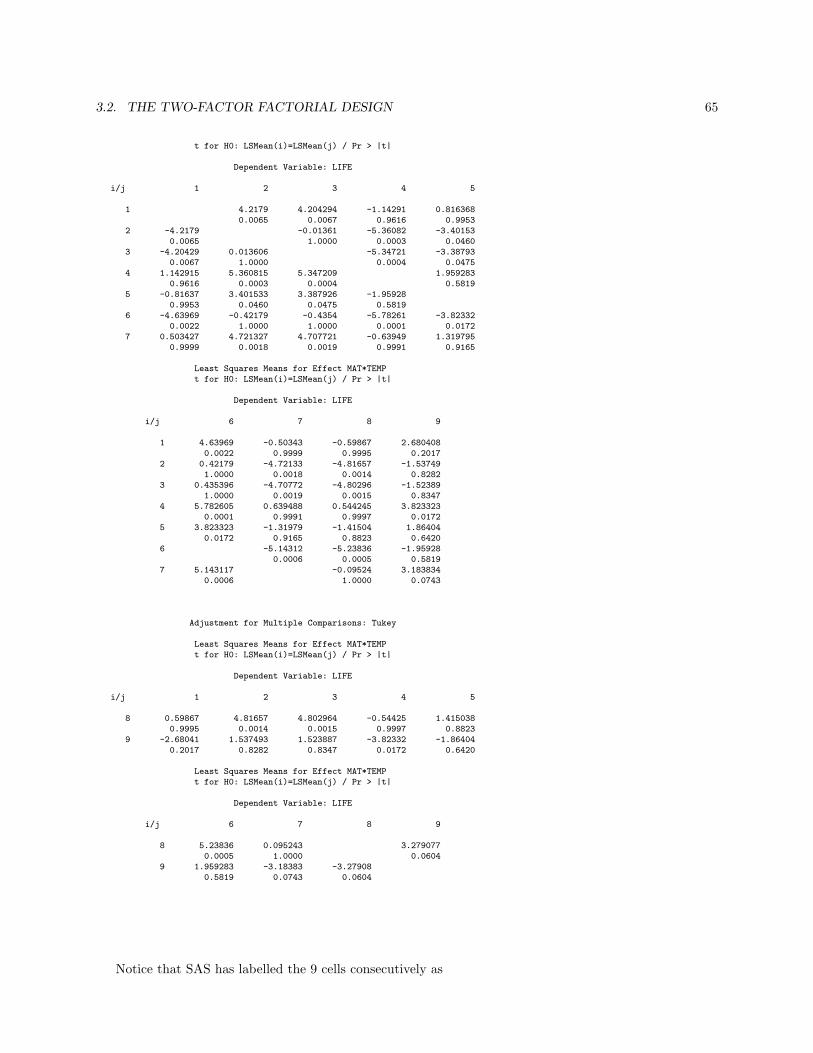
3.2. THE TWO-FACTOR FACTORIAL DESIGN 65
t for H0: LSMean(i)=LSMean(j) / Pr > |t|
Dependent Variable: LIFE
i/j 1 2 3 4 5
1 4.2179 4.204294 -1.14291 0.8163680.0065 0.0067 0.9616 0.9953
2 -4.2179 -0.01361 -5.36082 -3.401530.0065 1.0000 0.0003 0.0460
3 -4.20429 0.013606 -5.34721 -3.387930.0067 1.0000 0.0004 0.0475
4 1.142915 5.360815 5.347209 1.9592830.9616 0.0003 0.0004 0.5819
5 -0.81637 3.401533 3.387926 -1.959280.9953 0.0460 0.0475 0.5819
6 -4.63969 -0.42179 -0.4354 -5.78261 -3.823320.0022 1.0000 1.0000 0.0001 0.0172
7 0.503427 4.721327 4.707721 -0.63949 1.3197950.9999 0.0018 0.0019 0.9991 0.9165
Least Squares Means for Effect MAT*TEMPt for H0: LSMean(i)=LSMean(j) / Pr > |t|
Dependent Variable: LIFE
i/j 6 7 8 9
1 4.63969 -0.50343 -0.59867 2.6804080.0022 0.9999 0.9995 0.2017
2 0.42179 -4.72133 -4.81657 -1.537491.0000 0.0018 0.0014 0.8282
3 0.435396 -4.70772 -4.80296 -1.523891.0000 0.0019 0.0015 0.8347
4 5.782605 0.639488 0.544245 3.8233230.0001 0.9991 0.9997 0.0172
5 3.823323 -1.31979 -1.41504 1.864040.0172 0.9165 0.8823 0.6420
6 -5.14312 -5.23836 -1.959280.0006 0.0005 0.5819
7 5.143117 -0.09524 3.1838340.0006 1.0000 0.0743
Adjustment for Multiple Comparisons: Tukey
Least Squares Means for Effect MAT*TEMPt for H0: LSMean(i)=LSMean(j) / Pr > |t|
Dependent Variable: LIFE
i/j 1 2 3 4 5
8 0.59867 4.81657 4.802964 -0.54425 1.4150380.9995 0.0014 0.0015 0.9997 0.8823
9 -2.68041 1.537493 1.523887 -3.82332 -1.864040.2017 0.8282 0.8347 0.0172 0.6420
Least Squares Means for Effect MAT*TEMPt for H0: LSMean(i)=LSMean(j) / Pr > |t|
Dependent Variable: LIFE
i/j 6 7 8 9
8 5.23836 0.095243 3.2790770.0005 1.0000 0.0604
9 1.959283 -3.18383 -3.279080.5819 0.0743 0.0604
Notice that SAS has labelled the 9 cells consecutively as

66 CHAPTER 3. FACTORIAL DESIGNS
1 2 34 5 67 8 9
We use underlining to summarize the results.Temperature within Material:
Material = 1 y12. y13. y11.
57.25 57.50 134.75
Material = 2 y23. y22. y21.
49.50 119.75 155.75
Material = 3 y33. y31. y32.
85.5 144.00 145.75
Material within Temperature:
Temperature = 1 y11. y31. y21.
134.75 144.00 155.75
Temperature = 2 y12. y22. y32.
57.25 119.75 145.75
Temperature = 3 y23. y13. y33.
49.50 57.50 85.5
Model Diagnostics
Diagnostics are run the usual way via residual analysis. Recall that the residuals for the two-factor factorialmodel are given by
eijk = yijk − yij.
Graphical checks for equality of variances as well as unusual observations are plots of residuals versus
• yij.,
• factor A, and
• factor B.
The graphical check for normality is the QQ-plot of the residuals. For the battery life example thefollowing SAS code may be used to produce the required plots.
PROC GLM;CLASS MAT TEMP;MODEL LIFE=MAT TEMP MAT*TEMP;OUTPUT OUT=DIAG R=RES P=PRED;
RUN;QUIT;
SYMBOL V=CIRCLE;PROC UNIVARIATE NOPRINT;
QQPLOT RES / NORMAL (L=1 MU=0 SIGMA=EST);HIST RES / NORMAL (L=1 MU=0 SIGMA=EST);
RUN;QUIT;
PROC GPLOT;PLOT RES*MAT;PLOT RES*TEMP;PLOT RES*PRED;
RUN;QUIT;

3.2. THE TWO-FACTOR FACTORIAL DESIGN 67
Formal tests for normality indicate no deviation from normality. The QQ-plot shows no signs of non-normality. The residual plots show a mild deviation from constant variance. We may need to transform thedata.
Goodness-of-Fit Tests for Normal Distribution
Test ---Statistic---- -----p Value-----
Cramer-von Mises W-Sq 0.05586092 Pr > W-Sq >0.250Anderson-Darling A-Sq 0.34769847 Pr > A-Sq >0.250
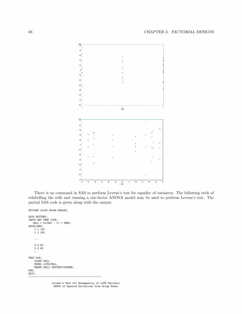
68 CHAPTER 3. FACTORIAL DESIGNS
There is no command in SAS to perform Levene’s test for equality of variances. The following trick ofrelabelling the cells and running a one-factor ANOVA model may be used to perform Levene’s test. Thepartial SAS code is given along with the output.
OPTIONS LS=80 PS=66 NODATE;
DATA BATTERY;INPUT MAT TEMP LIFE;
CELL = 3*(MAT - 1) + TEMP;DATALINES;
1 1 1301 1 155
...
3 3 823 3 60;
PROC GLM;CLASS CELL;MODEL LIFE=CELL;MEANS CELL/ HOVTEST=LEVENE;
RUN;QUIT;--------------------------------------------------
Levene’s Test for Homogeneity of LIFE VarianceANOVA of Squared Deviations from Group Means

3.2. THE TWO-FACTOR FACTORIAL DESIGN 69
Sum of MeanSource DF Squares Square F Value Pr > FCELL 8 5407436 675929 1.48 0.2107Error 27 12332885 456774

70 CHAPTER 3. FACTORIAL DESIGNS
3.2.2 Random and Mixed Models
We shall now consider the case where the levels of factor A or the levels of factor B are randomly chosenfrom a population of levels.
The Random Effects Model
In a random effects model the a levels of factor A and the b levels of factor B are random samples frompopulations of levels. The statistical model is the same as the one given in (3.1) where τi, βj , (τβ)ij , and εijk
are randomly sampled from N(0, σ2τ ), N(0, σ2
β),N(0, σ2τβ), and N(0, σ2) distributions, respectively. Thus, the
variance of any observation isV ar(yijk) = σ2
τ + σ2β + σ2
τβ + σ2
The hypotheses of interest areA main effect:
H0 : σ2τ = 0
HA : σ2τ 6= 0
B main effect:
H0 : σ2β = 0
HA : σ2β 6= 0
AB interaction effect:
H0 : σ2τβ = 0
HA : σ2τβ 6= 0
The ANOVA table needs some modifications. This is seen examining the expected mean squares.
E(MSA) = σ2 + nσ2τβ + bnσ2
τ
E(MSB) = σ2 + nσ2τβ + anσ2
β
E(MSAB) = σ2 + nσ2τβ
E(MSE) = σ2
Therefore, the two-factor random effects ANOVA table is:
Source df SS MS F -statistic
A a− 1 SSA MSA FA = MSAMSAB
B b− 1 SSB MSB FB = MSBMSAB
AB (a− 1)(b− 1) SSAB MSAB FAB = MSABMSE
Error ab(n− 1) SSE MSE
Total abn− 1 SST
From the expected mean squares, we get the estimates of the variance components as
σ2 = MSE
σ2τβ =
MSAB −MSE
n
σ2τ =
MSA −MSAB
bn
σ2β =
MSB −MSAB
an

3.2. THE TWO-FACTOR FACTORIAL DESIGN 71
Example
Consider the battery life example once again. This time assume that the material types and temperaturesare randomly selected out of several possibilities. We may then use the RANDOM statement in PROCGLM of SAS to analyze the data as a random effects model. Here are the SAS code and associated output.
OPTIONS LS=80 PS=66 NODATE;
DATA BATTERY;INPUT MAT TEMP LIFE;DATALINES;
1 1 1301 1 155.......
3 3 60;
PROC GLM;CLASS MAT TEMP;MODEL LIFE=MAT TEMP MAT*TEMP;RANDOM MAT TEMP MAT*TEMP / TEST;
RUN;QUIT;
---------------------------------------------------------
The GLM Procedure
Source Type III Expected Mean Square
MAT Var(Error) + 4 Var(MAT*TEMP) + 12 Var(MAT)
TEMP Var(Error) + 4 Var(MAT*TEMP) + 12 Var(TEMP)
MAT*TEMP Var(Error) + 4 Var(MAT*TEMP)
The GLM ProcedureTests of Hypotheses for Random Model Analysis of Variance
Dependent Variable: LIFE
Source DF Type III SS Mean Square F Value Pr > F
MAT 2 10684 5341.861111 2.22 0.2243TEMP 2 39119 19559 8.14 0.0389
Error: MS(MAT*TEMP) 4 9613.777778 2403.444444
Source DF Type III SS Mean Square F Value Pr > F
MAT*TEMP 4 9613.777778 2403.444444 3.56 0.0186
Error: MS(Error) 27 18231 675.212963
Notice that variability among material types is the only factor that is not significant.The estimates of the components of variance are (values in parentheses are percent contributions of the
components)
σ2 = MSE = 675.21 (24.27%)
σ2τβ =
MSAB −MSE
n=
2403.44− 675.214
= 432.06 (15.53%)
σ2τ =
MSA −MSAB
bn=
5341.86− 2403.4412
= 244.87 (8.80%)
σ2β =
MSB −MSAB
an=
19559− 2403.4412
= 1429.58 (51.39%)

72 CHAPTER 3. FACTORIAL DESIGNS
Mixed Models
Let us now consider the case where one factor is fixed and the other is random. Without loss of generality,assume that factor A is fixed and factor B is random. When a factor is random, its interaction with anyother factor is also random.
The statistical model, once again, has the same form given in (3.1). This time we assume that
• τi are fixed effects such that∑
τi = 0,
• βj ∼iid N(0, σ2β), (τβ)ij ∼iid N(0, a−1
a σ2τβ), and εijk ∼iid N(0, σ2).
The hypotheses of interest are
H0 : τ1 = · · · = τa = 0, H0 : σ2β = 0, H0 : σ2
τβ = 0
The expected mean squares are given by
E(MSA) = σ2 + nσ2τβ +
bn∑
τ2i
a− 1E(MSB) = σ2 + anσ2
β
E(MSAB) = σ2 + nσ2τβ
E(MSE) = σ2
The fixed factor effects are estimated the usual way as
µ = y..., τi = yi.. − y...
and the variance components are estimated as
σ2 = MSE , σ2τβ =
MSAB −MSE
n, and σ2
β =MSB −MSE
an
The ANOVA table for the mixed model is
Source df SS MS F -statistic
A (fixed) a− 1 SSA MSA FA = MSAMSAB
B (random) b− 1 SSB MSB FB = MSBMSE
AB (a− 1)(b− 1) SSAB MSAB FAB = MSABMSE
Error ab(n− 1) SSE MSE
Total abn− 1 SST
Example
Consider the battery life example and assume that temperature is a random factor while material type is afixed factor. We use PROC MIXED in SAS to generate the output. PROC GLM does not provide thecorrect analysis!
OPTIONS LS=80 PS=66 NODATE;
DATA BATTERY;INPUT MAT TEMP LIFE;DATALINES;
1 1 1301 1 155.......
3 3 60;
PROC MIXED COVTEST;CLASS MAT TEMP;

3.2. THE TWO-FACTOR FACTORIAL DESIGN 73
MODEL LIFE=MAT;RANDOM TEMP MAT*TEMP;
RUN;QUIT;
-----------------------------------------------------------------------
The Mixed Procedure
Model Information
Data Set WORK.BATTERYDependent Variable LIFECovariance Structure Variance ComponentsEstimation Method REMLResidual Variance Method ProfileFixed Effects SE Method Model-BasedDegrees of Freedom Method Containment
Class Level Information
Class Levels Values
MAT 3 1 2 3TEMP 3 1 2 3
Dimensions
Covariance Parameters 3Columns in X 4Columns in Z 12Subjects 1Max Obs Per Subject 36Observations Used 36Observations Not Used 0Total Observations 36
Iteration History
Iteration Evaluations -2 Res Log Like Criterion
0 1 352.412588551 1 327.91147422 0.00000000
Convergence criteria met.
Covariance Parameter Estimates
Standard ZCov Parm Estimate Error Value Pr Z
TEMP 1429.66 1636.09 0.87 0.1911MAT*TEMP 432.06 427.35 1.01 0.1560Residual 675.21 183.77 3.67 0.0001
Fit Statistics
-2 Res Log Likelihood 327.9AIC (smaller is better) 333.9AICC (smaller is better) 334.7BIC (smaller is better) 331.2
The Mixed Procedure
Type 3 Tests of Fixed Effects
Num DenEffect DF DF F Value Pr > F
MAT 2 4 2.22 0.2243

74 CHAPTER 3. FACTORIAL DESIGNS
From the output we observe that the fixed effect (MAT) is not significant. Neither of the random effectsare significant (p-values of 0.1911 and 0.1560).
Proc Mixed uses the restricted maximum likelihood (REML) technique to estimate the variance compo-nents. In a balanced design the REML method gives identical estimates as those obtained using the expectedmean squares. When there is imbalance, however, the results are not the same.
Exercise: For this example, show that the estimates of the variance components obtained here are identicalto those using the expected mean squares.

3.3. BLOCKING IN FACTORIAL DESIGNS 75
3.3 Blocking in Factorial Designs
Blocking may be implemented in factorial designs using the same principles. In a randomized block design,every block contains all possible treatment combinations.
The statistical model for a two-factor blocked factorial design with 1 replication per block is
yijk = µ + τi + βj + (τβ)ij + δk + εijk
where i = 1, · · · , a, j = 1, · · · , b, and k = 1, · · · , n. δk is the effect of the kth block.The model assumes that treatment-block interactions are negligible. The ANOVA table for a random
effects model is
Source df SS MS F -statisticA a− 1 SSA MSA FA = MSA
MSAB
B b− 1 SSB MSB FB = MSB
MSAB
AB (a− 1)(b− 1) SSAB MSAB FAB = MSAB
MSE
Blocks n− 1 SSBlocks MSBlocksError (ab− 1)(n− 1) SSE MSE
Total abn− 1 SST
where
SSBlocks = ab
n∑
k=1
(y..k − y...)2 .
Example
An agronomist wanted to study the effect of different rates of phosphorous fertilizer on two types of broadbean plants. He thought that the plant types might respond differently to fertilization; so, he decided to doa factorial experiment with two factors:
1. Plant type (T ) at two levels
• T1 = short, bushy• T2 = tall, erect
2. Phosphorous rate (P ) at three levels
• P1 = none• P2 = 25kg/ha
• P3 = 50kg/ha
Using the full factorial set of combinations he had six treatments:
T1P1, T1P2, T1P3, T2P1, T2P2, T2P3
He conducted the experiment using a randomized block design with four blocks of six plots each. Thefield layout and the yield in kg/ha are shown below:
BLOCKI II III IV
T2P2(8.3) T2P1(11.2) T1P2(17.6) T1P3(18.9)T2P1(11.0) T2P2(10.5) T1P1(14.3) T2P2(12.8)T1P1(11.5) T2P3(16.7) T2P1(12.1) T2P3(17.5)T2P3(15.7) T1P2(17.6) T1P3(18.2) T2P1(12.6)T1P3(18.2) T1P1(13.6) T2P3(16.6) T1P2(18.1)T1P2(17.1) T1P3(17.6) T2P2(9.1) T1P1(14.5)

76 CHAPTER 3. FACTORIAL DESIGNS
The data layout is (observations in a cell are in increasing block order I, II, III, IV)
PhosphorousType P1 P2 P3
T1 11.5, 13.6, 14.3, 14.5 17.1, 17.6, 17.6, 18.1 18.2, 17.6, 18.2, 18.9T2 11.0, 11.2, 12.1, 12.6 8.3, 10.5, 9.1, 12.8 15.7, 16.7, 16.6, 17.5
The following SAS code and output give the analysis.
3.3. BLOCKING IN FACTORIAL DESIGNS 77
OPTIONS LS=80 PS=66 NODATE;
DATA FERT;INPUT TYPE PH BLOCK YIELD;DATALINES;
1 1 1 11.51 1 2 13.61 1 3 14.31 1 4 14.51 2 1 17.11 2 2 17.61 2 3 17.61 2 4 18.11 3 1 18.21 3 2 17.61 3 3 18.21 3 4 18.92 1 1 11.02 1 2 11.22 1 3 12.12 1 4 12.62 2 1 8.32 2 2 10.52 2 3 9.12 2 4 12.82 3 1 15.72 3 2 16.72 3 3 16.62 3 4 17.5
;
PROC GLM;CLASS TYPE PH BLOCK;MODEL YIELD=BLOCK TYPE|PH;
RUN;QUIT;

78 CHAPTER 3. FACTORIAL DESIGNS
-------------------------------------------------
The GLM Procedure
Dependent Variable: YIELD
Sum ofSource DF Squares Mean Square F Value Pr > F
Model 8 234.7000000 29.3375000 50.72 <.0001
Error 15 8.6762500 0.5784167
Corrected Total 23 243.3762500
R-Square Coeff Var Root MSE YIELD Mean
0.964350 5.195813 0.760537 14.63750
Source DF Type I SS Mean Square F Value Pr > F
BLOCK 3 13.32125000 4.44041667 7.68 0.0024TYPE 1 77.40041667 77.40041667 133.81 <.0001PH 2 99.87250000 49.93625000 86.33 <.0001TYPE*PH 2 44.10583333 22.05291667 38.13 <.0001
Source DF Type III SS Mean Square F Value Pr > F
BLOCK 3 13.32125000 4.44041667 7.68 0.0024TYPE 1 77.40041667 77.40041667 133.81 <.0001PH 2 99.87250000 49.93625000 86.33 <.0001TYPE*PH 2 44.10583333 22.05291667 38.13 <.0001
The interaction between plant type and phosphorous level is significant. This means that all comparisonsof means of one factor would have to be done within the levels of the other factor. Different plant typesrespond differently to different levels of the fertilizer. Short, bushy plants seem to show their greatest yieldincrease with the first increment of added phosphorous, while tall, erect plants seem to show no yield increasewith 25kg/ha of phosphorous.
Blocking seems to be working here judging from the corresponding F value. The efficiency needs to beinvestigated further.
The main effects are also significant. The rates of phosphorous fertilizer and the type of plant both affectyield significantly.

3.4. THE GENERAL FACTORIAL DESIGN 79
A Factorial Experiment with Two Blocking Factors
This is dealt with by implementing a Latin square design in a similar manner as one factor experiments.The only difference here is that every factor combination is considered to be a treatment. To illustrate this,consider a two-factor factorial experiment with 3 levels of factor A and 2 levels of factor B. We will useLatin letters to represent the 3× 2 = 6 treatment combinations.
A B TreatmentA1 B1 AA1 B2 BA2 B1 CA2 B2 DA3 B1 EA3 B2 F
We then form the 6× 6 basic Latin square cyclically as
ColumnRow 1 2 3 4 5 6
1 A B C D E F2 B C D E F A3 C D E F A B3 D E F A B C3 E F A B C D3 F A B C D E
We then randomize the rows and the columns.In general, consider two factors : factor A with a levels and factor B with b levels. The statistical model
is
yijkl = µ + τi + βj + γk + δl + (τβ)ij + εijkl
where
• τi, i = 1, · · · , a is the effect of the ith level of factor A,
• βj , j = 1, · · · , b is the effect of the jth level of factor B,
• γk and δl, k, l = 1, · · · , ab, are the effects of the kth row and the lth column, respectively.
3.4 The General Factorial Design
Consider an experiment in which we have t factors F1, · · · , Ft with f1, · · · , ft levels, respectively. Thestatistical model is
yi1i2···itl = µ + τ1i1+ τ2i2
+ · · ·+ τtit
+ (τ1τ2)i1i2 + · · · (τt−1τt)it−1it
+ · · ·+ (τ1τ2 · · · τt)i1i2···it + εi1i2···itl
where i1 = 1, · · · , f1; i2 = 1, · · · , f2, etc.A special case is the 3 factor factorial design with factors A, B, and C with levels a, b, and c, respectively.
We need two or more replications to be able to test for all possible interactions. The statistical model is
yijkl = µ + τi + βj + γk + (τβ)ij + (τγ)ik + (βγ)jk + (τβγ)ijk + εijkl
where i = 1, · · · , a; j = 1, · · · , b; k = 1, · · · , c; and l = 1, · · · , n.Considering a fixed effects model, the ANOVA table is

80 CHAPTER 3. FACTORIAL DESIGNS
Source df SS MS F -statistic
A a− 1 SSA MSA FA = MSAMSE
B b− 1 SSB MSB FB = MSBMSE
C c− 1 SSC MSC FC = MSCMSE
AB (a− 1)(b− 1) SSAB MSAB FAB = MSABMSE
AC (a− 1)(c− 1) SSAC MSAC FAC = MSACMSE
BC (b− 1)(c− 1) SSBC MSBC FBC = MSBCMSE
ABC (a− 1)(b− 1)(c− 1) SSABC MSABC FABC = MSABCMSE
Error abc(n− 1) SSE MSE
Total abcn− 1 SST
The following example is taken from Montgomery : Design and Analysis of Experiments
Example
A soft drink bottler is studying the effect of percent carbonation (A), operating pressure (B), and line speed(C) on the volume of beverage packaged in each bottle. Three levels of A, two levels of B and two levels ofC are considered to set up a 3× 2× 2 factorial experiment. This experiment is run twice and the deviationsfrom the target volume are recorded. The data are given below.
Pressure (B)25 psi 30 psi
Line Speed (C) Line Speed (C)Carbonation (A) 200 250 200 250
10 -3, -1 -1, 0 -1, 0 1, 112 0, 1 2, 1 2, 3 6, 514 5, 4 7, 6 7, 9 10, 11
We will use SAS to analyze the data. The SAS code and output are as follows:
OPTIONS LS=80 PS=66 NODATE;DATA BOTTLE;INPUT CARB PRES SPEED VOL;CARDS;
1 1 1 -31 1 1 -11 1 2 -11 1 2 01 2 1 -11 2 1 01 2 2 11 2 2 12 1 1 02 1 1 12 1 2 22 1 2 12 2 1 22 2 1 32 2 2 62 2 2 53 1 1 53 1 1 43 1 2 73 1 2 63 2 1 73 2 1 93 2 2 103 2 2 11
;
PROC GLM;CLASS CARB PRES SPEED;MODEL VOL = CARB|PRES|SPEED;
RUN;

3.4. THE GENERAL FACTORIAL DESIGN 81
QUIT;
-------------------------------------------------------------
Sum ofSource DF Squares Mean Square F Value Pr > F
Model 11 328.1250000 29.8295455 42.11 <.0001Error 12 8.5000000 0.7083333Corrected Total 23 336.6250000
Source DF Type I SS Mean Square F Value Pr > F
CARB 2 252.7500000 126.3750000 178.41 <.0001PRES 1 45.3750000 45.3750000 64.06 <.0001CARB*PRES 2 5.2500000 2.6250000 3.71 0.0558SPEED 1 22.0416667 22.0416667 31.12 0.0001CARB*SPEED 2 0.5833333 0.2916667 0.41 0.6715PRES*SPEED 1 1.0416667 1.0416667 1.47 0.2486CARB*PRES*SPEED 2 1.0833333 0.5416667 0.76 0.4869
As we can see, none of the interactions is significant. However, all the main effects appear to be significant.One may perform multiple comparisons at the highest level of the factors. As an example we will run theTukey-Kramer procedure on factor A. PROC GLM of SAS is modified as follows:
PROC GLM;CLASS CARB PRES SPEED;MODEL VOL = CARB|PRES|SPEED;LSMEANS CARB/PDIFF ADJUST=TUKEY;
RUN;QUIT;---------------------------------------------------------------
Adjustment for Multiple Comparisons: Tukey
LSMEANCARB VOL LSMEAN Number
1 -0.50000000 12 2.50000000 23 7.37500000 3
Least Squares Means for effect CARBPr > |t| for H0: LSMean(i)=LSMean(j)
Dependent Variable: VOL
i/j 1 2 31 <.0001 <.00012 <.0001 <.00013 <.0001 <.0001
Thus, all pairwise comparisons comparisons of the levels of factor A, percent carbonation, are significantlydifferent at MEER = 0.05.

82 CHAPTER 3. FACTORIAL DESIGNS

Chapter 4
2k and 3k Factorial Designs
4.1 Introduction
Often we consider general factorial designs with k factors each with 2 levels, denoted by + and −. Thisinvolves a 2×2×· · ·×2 = 2k factorial experiment. This is known as a 2k factorial design. A similar situationwhere each of the k factors has three levels (0, 1, 2) is known as a 3k factorial design.
4.2 The 2k Factorial Design
This is particularly useful in the early stages of an experiment as a factor screening mechanism, i.e. toidentify important factors. Every interaction term has only 1 degree of freedom. We shall consider specialcases where k = 2, 3 before looking at the general 2k factorial design.
4.2.1 The 22 Design
Let A and B denote the two factors of interest with two levels (”low (−)” and ”high (+)”) each. There are22 = 4 treatments designated as:
Treatment A B(1) − −a + −b − +ab + +
The presence of a letter indicates that the factor is at a high level. The absence of letter indicates thefactor is at a low level. The symbol (1) is used to represent the treatment where every factor is at a lowlevel.
As an example consider an experiment where the time a chemical reaction takes is investigated. The twofactors of interest are reactant concentration (A at 15% (−) and 25% (+)) and catalyst (B with absence (−)and presence (+)). The experiment is replicated three times.
Factor ReplicateA B Treatment 1 2 3 Total− − (1) 28 25 27 80+ − a 36 32 32 100− + b 18 19 23 60+ + ab 31 30 29 90
83

84 CHAPTER 4. 2K AND 3K FACTORIAL DESIGNS
Let y(A+) denote the mean of the response where factor A is at high level. A similar notation is use forall the other means. For example, y(A−B+) is the mean of the response in the case where factor A is at lowlevel and factor B is at high level.
We can now define the main effects of a factor. The main effect of A is
y(A+)− y(A−)
This is equivalent to
12{y(A+B+) + y(A+B−)} − 1
2{y(A−B+) + y(A−B−)} = 8.33
Using the treatment means, this may be given as a contrast with coefficients (−.5, .5,−.5, .5).Similarly, the main effect of B is given by
y(B+)− y(B−)
which is equivalent to
12{y(A+B+) + y(A−B+)} − 1
2{y(A+B−) + y(A−B−)} = −5.00
Now the contrast coefficients are (−.5,−.5, .5, .5).The AB interaction effect is the average difference between the effect of A at the high level of B and the
effect of A at the low level of B
12{y(A+B+)− y(A−B+)} − 1
2{y(A+B−)− y(A−B−)} = 1.67
Using the treatment means, the contrast coefficients become (.5,−.5,−.5, .5).The sum of squares for each factor and the interaction may be obtained in a very simple manner. Let n
be the number of replicates in the study.
SSA = n× (Main effect of A)2
SSB = n× (Main effect of B)2
SSAB = n× (Interaction effect of AB)2
The total sum of squares is defined as usual
SST =2∑
i=1
2∑
j=1
n∑
k=1
(yijk − y...)2
and the error sum of squares is obtained by subtraction as
SSE = SST − SSA − SSB − SSAB .
For the example above these yield
SSA = 208.33, SSB = 75.00, SSAB = 8.33, SST = 323.00, SSE = 31.34
The ANOVA table is
Source df SS MS F -statistic
A 1 SSA = 208.33 MSA = 208.33 FA = MSAMSE
= 53.15
B 1 SSB = 75.00 MSB = 75.00 FB = MSBMSE
= 19.13
AB 1 SSAB = 8.33 MSAB = 8.33 FAB = MSABMSE
= 2.13
Error 4(n− 1) = 8 SSE = 31.34 MSE = 3.92
Total 4n− 1 = 11 SST = 323.00

4.2. THE 2K FACTORIAL DESIGN 85
Using SAS
OPTIONS LS=80 PS=66 NODATE;DATA BOTTLE;INPUT A B Y @@;CARDS;
-1 -1 28 -1 -1 25 -1 -1 271 -1 36 1 -1 32 1 -1 32-1 1 18 -1 1 19 -1 1 231 1 31 1 1 30 1 1 29
;
PROC GLM;CLASS A B;MODEL Y = A|B;
RUN;QUIT;
-----------------------------------------------
Source DF Type I SS Mean Square F Value Pr > F
A 1 208.3333333 208.3333333 53.19 <.0001B 1 75.0000000 75.0000000 19.15 0.0024A*B 1 8.3333333 8.3333333 2.13 0.1828
One may use a multiple regression model to estimate the effects in a 22 design. This is done by formingtwo variables (x1, x2) as
A− x1 = −.5A+ x1 = .5B− x2 = −.5B+ x2 = .5
and fitting the regression model
y = β0 + β1x1 + β2x2 + β12(2x1x2) + ε .
The estimated model coefficient are now
β0 = y...
β1 = Main effect of A
β2 = Main effect of B
β12 = AB Interaction effect
Using SAS
OPTIONS LS=80 PS=66 NODATE;DATA BOTTLE;INPUT A B Y @@;X1 = A/2;X2 = B/2;X1X2 = 2*X1*X2;CARDS;
-1 -1 28 -1 -1 25 -1 -1 271 -1 36 1 -1 32 1 -1 32-1 1 18 -1 1 19 -1 1 231 1 31 1 1 30 1 1 29
;
PROC GLM;MODEL Y = X1 X2 X1X2;
RUN;QUIT;
----------------------------------------

86 CHAPTER 4. 2K AND 3K FACTORIAL DESIGNS
Dependent Variable: Y
Sum ofSource DF Squares Mean Square F Value Pr > F
Model 3 291.6666667 97.2222222 24.82 0.0002
Error 8 31.3333333 3.9166667
Corrected Total 11 323.0000000
R-Square Coeff Var Root MSE Y Mean
0.902993 7.196571 1.979057 27.50000
Source DF Type I SS Mean Square F Value Pr > F
X1 1 208.3333333 208.3333333 53.19 <.0001X2 1 75.0000000 75.0000000 19.15 0.0024X1X2 1 8.3333333 8.3333333 2.13 0.1828
StandardParameter Estimate Error t Value Pr > |t|
Intercept 27.50000000 0.57130455 48.14 <.0001X1 8.33333333 1.14260910 7.29 <.0001X2 -5.00000000 1.14260910 -4.38 0.0024X1X2 1.66666667 1.14260910 1.46 0.1828
4.2.2 The 23 Design
In this subsection we consider 3-factor factorial experiments each with two levels. This setup uses a total of23 = 8 experiments that are represented as
Treatment A B C Treatment A B C(1) − − − c − − +a + − − ac + − +b − + − bc − + +c − c + abc + + +
The following table gives the contrast coefficients for calculating the effects.
Factorial EffectsTreatment I A B AB C AC BC ABC
(1) 1/4 -1/4 -1/4 1/4 -1/4 1/4 1/4 -1/4a 1/4 1/4 -1/4 -1/4 -1/4 -1/4 1/4 1/4b 1/4 -1/4 1/4 -1/4 -1/4 1/4 -1/4 1/4ab 1/4 1/4 1/4 1/4 -1/4 -1/4 -1/4 -1/4c 1/4 -1/4 -1/4 1/4 1/4 -1/4 -1/4 1/4ac 1/4 1/4 -1/4 -1/4 1/4 1/4 -1/4 -1/4bc 1/4 -1/4 1/4 -1/4 1/4 -1/4 1/4 -1/4abc 1/4 1/4 1/4 1/4 1/4 1/4 1/4 1/4
For example, the main effect of A is
14[−y(A−B−C−) + y(A+B−C−)− y(A−B+C−) + y(A+B+C−)
−y(A−B−C+) + y(A+B−C+)− y(A−B+C+) + y(A+B+C+)]
The sum of squares areSSeffect = 2n(effect)2
Consider the bottling experiment in Chapter 3. With only the first two levels of factor A, the data is
4.2. THE 2K FACTORIAL DESIGN 87
Pressure (B)25 psi 30 psi
Line Speed (C) Line Speed (C)Carbonation (A) 200 250 200 250
10 (1): -3, -1 c: -1, 0 b: -1, 0 bc: 1, 112 a: 0, 1 ac: 2, 1 ab: 2, 3 abc: 6, 5
The SAS analysis is given below:
OPTIONS LS=80 PS=66 NODATE;DATA BOTTLE;INPUT A B C VOL;CARDS;
-1 -1 -1 -3-1 -1 -1 -1-1 -1 1 -1-1 -1 1 0-1 1 -1 -1-1 1 -1 0-1 1 1 1-1 1 1 11 -1 -1 01 -1 -1 11 -1 1 21 -1 1 11 1 -1 21 1 -1 31 1 1 61 1 1 5
;
PROC GLM;CLASS A B C;MODEL VOL = A|B|C;
RUN;QUIT;
---------------------------------------------------
Sum ofSource DF Squares Mean Square F Value Pr > F
Model 7 73.00000000 10.42857143 16.69 0.0003Error 8 5.00000000 0.62500000
Corrected Total 15 78.00000000
R-Square Coeff Var Root MSE VOL Mean0.935897 79.05694 0.790569 1.000000
Source DF Type I SS Mean Square F Value Pr > F
A 1 36.00000000 36.00000000 57.60 <.0001B 1 20.25000000 20.25000000 32.40 0.0005A*B 1 2.25000000 2.25000000 3.60 0.0943C 1 12.25000000 12.25000000 19.60 0.0022A*C 1 0.25000000 0.25000000 0.40 0.5447B*C 1 1.00000000 1.00000000 1.60 0.2415A*B*C 1 1.00000000 1.00000000 1.60 0.2415
To employ multiple regression, one may consider the following coding:
A− x1 = −.5A+ x1 = .5B− x2 = −.5B+ x2 = .5C− x3 = −.5C+ x3 = .5

88 CHAPTER 4. 2K AND 3K FACTORIAL DESIGNS
The regression model is
y = β0 + β1x1 + β2x2 + β3x3 + β12(2x1x2) + β13(2x1x3)
+β23(2x2x3) + β123(4x1x2x3) + ε
Once again, the estimate of the regression coefficients correspond to the effects of the factors. Forexample, β12 is the AB interaction effect. Considering the bottling experiment, the following SAS code isan implementation the regression approach.OPTIONS LS=80 PS=66 NODATE;DATA BOTTLE;INPUT A B C VOL;X1 = A/2;X2 = B/2;X3 = C/2;X1X2 = 2*X1*X2;X1X3 = 2*X1*X3;X2X3 = 2*X2*X3;X1X2X3 = 4*X1*X2*X3;CARDS;
-1 -1 -1 -3-1 -1 -1 -1-1 -1 1 -1-1 -1 1 0-1 1 -1 -1-1 1 -1 0-1 1 1 1-1 1 1 11 -1 -1 01 -1 -1 11 -1 1 21 -1 1 11 1 -1 21 1 -1 31 1 1 61 1 1 5
;
PROC REG;MODEL VOL = X1 X2 X3 X1X2 X1X3 X2X3 X1X2X3;
RUN;QUIT;
---------------------------------------------------Dependent Variable: VOL
Analysis of Variance
Sum of MeanSource DF Squares Square F Value Pr > F
Model 7 73.00000 10.42857 16.69 0.0003Error 8 5.00000 0.62500Corrected Total 15 78.00000
Root MSE 0.79057 R-Square 0.9359Dependent Mean 1.00000 Adj R-Sq 0.8798Coeff Var 79.05694
Parameter Estimates
Parameter StandardVariable DF Estimate Error t Value Pr > |t|
Intercept 1 1.00000 0.19764 5.06 0.0010X1 1 3.00000 0.39528 7.59 <.0001X2 1 2.25000 0.39528 5.69 0.0005X3 1 1.75000 0.39528 4.43 0.0022X1X2 1 0.75000 0.39528 1.90 0.0943X1X3 1 0.25000 0.39528 0.63 0.5447X2X3 1 0.50000 0.39528 1.26 0.2415X1X2X3 1 0.50000 0.39528 1.26 0.2415

4.2. THE 2K FACTORIAL DESIGN 89
One may obtain sums of squares using
SS = 2n(effect)2 .
For example, in the bottling experiment,
SSA = 2× 2× 32 = 36 .
4.2.3 The General 2k Design
Consider k factors F1, · · · , Fk each with 2 levels. Suppose the experiment is replicated n times. There arek =
(k1
)main effects,
(k2
)two-factor interaction effects,
(k3
)three-factor interaction effects, . . . ,
(kk
)= 1
k-factor interaction. Each main effect as well as interaction effect has one degree of freedom. Thus the sumof the degrees of freedom due to the factors (main and interaction) is
k∑
i=1
(k
i
)= 2k − 1
and the total degrees of freedom are 2kn− 1. Thus we get the error degrees of freedom to be
(2kn− 1)− (2k − 1) = 2k(n− 1) .
The partial ANOVA table for the 2k design is
Source df SS
k main effectsF1 1 SSF1
F1 1 SSF1
......
...Fk 1 SSFk�
k2
�two-factor interactions
F1F2 1 SSF1F2
F1F3 1 SSF1F3
......
...Fk−1Fk 1 SSFk−1Fk
......
...�kk
�= 1 k-factor interaction
F1F2 · · ·Fk 1 SSF1F2···Fk
Error 2k(n− 1) SSE
Total 2kn− 1 SST
We denote the 2k treatments using the standard notation, i.e.
(1), f1, · · · , f1 . . . fk .
As always contrasts are of interest since they represent factor effects. We will use contrast coefficients±21−k to linearly combine the 2k cell means. For instance, in the 22 design (k = 2), the coefficients are±21−2 = ±2−1 = ±1/2. Similarly, in the 23 design, the coefficients become ±1/4 as expected.
The sums of squares are nowSSeffect = n× 2k−2 × (effect)2 .
We will use the regression approach to estimate the effects. We will now create k variables x1, · · · , xk
each taking values ±1/2 depending on whether the corresponding factor is at high or low level. We then fitthe regression equation
y = β0 + β1x1 + · · ·+ βkxk + β12(2x1x2) + · · ·+ βk−1,k(2xk−1xk) + . . .

90 CHAPTER 4. 2K AND 3K FACTORIAL DESIGNS
+β12···k(2k−1x1x2 · · ·xk) + ε .
The multiplier is obtained as2(number of factors in interaction−1) .
Now the estimates, β’s, are the effects of the corresponding factor.
4.2.4 The Unreplicated 2k Design
Since the number of factor level combinations in a 2k design may be large, it is often impossible to findenough subjects to replicate the design. In such a situation it is impossible to estimate the error; which inturn means that hypotheses cannot be tested. An approach is to ignore some high-order interactions, i.e.assume that interactions with three or higher factors do not exist. Another approach is to use a QQ-plot toidentify the significant factors.
The following example, taken from Petersen : Design and Analysis of Experiments, illustrates theseapproaches.
Example
A research chemist wanted to study the effect of a number of factors on the yield of a new high-impactplastic. The plastic is produced by mixing resin with an extender in a solvent. The process takes place in aheated reaction vat. The materials are allowed to react for a period of time, and the plastic settles to thebottom of the vat, filtered on a screen, and dried.
The chemist worked in a laboratory that contained 32 experimental vats and a filter and dryer with eachvat. He knew that he could run one trial per day in each vat. He decided to study five factors using a singlereplication of a 25 design. He selected the following factors:
• A = reaction temperature : 300◦C, 150◦C
• B = reaction time : 4hr, 2hr
• C = filter pressure : 1atm, 2atm
• D = drying temperature : 200◦C, 100◦C
• E = resin/extender ratio : 2/1, 1/1
The following table gives the results:
A B C D E Yield
-1 -1 -1 -1 -1 2461 -1 -1 -1 -1 303-1 1 -1 -1 -1 2761 1 -1 -1 -1 336-1 -1 1 -1 -1 2581 -1 1 -1 -1 344-1 1 1 -1 -1 2651 1 1 -1 -1 313-1 -1 -1 1 -1 2491 -1 -1 1 -1 310-1 1 -1 1 -1 3181 1 -1 1 -1 363-1 -1 1 1 -1 2121 -1 1 1 -1 249-1 1 1 1 -1 2831 1 1 1 -1 219-1 -1 -1 -1 1 3791 -1 -1 -1 1 326-1 1 -1 -1 1 3441 1 -1 -1 1 349-1 -1 1 -1 1 3891 -1 1 -1 1 359-1 1 1 -1 1 2831 1 1 -1 1 363

4.2. THE 2K FACTORIAL DESIGN 91
-1 -1 -1 1 1 3131 -1 -1 1 1 336-1 1 -1 1 1 3701 1 -1 1 1 336-1 -1 1 1 1 3221 -1 1 1 1 352-1 1 1 1 1 3671 1 1 1 1 374
We will fit the following regression model to estimate the effects:
y = β0 + β1x1 + · · ·+ β12345(24x1x2x3x4x5) + ε
We save the above data as it is in a file called chem.dat, without the line which contains the names ofthe variables, and we call the file using the SAS command infile. The following code gives the analysis:
OPTIONS LS=80 PS=66 NODATE;
DATA CHEM;
INFILE "C:\ASH\S7010\SAS\CHEM.DAT";
INPUT A B C D E YIELD;
RUN;
QUIT;
DATA CHEM2;
SET CHEM;
AB=A*B; AC=A*C; AD=A*D; AE=A*E;
BC=B*C; BD=B*D; BE=B*E;
CD=C*D; CE=C*E;
DE=D*E;
ABC=A*B*C; ABD=A*B*D; ABE=A*B*E; ACD=A*C*D; ACE=A*C*E; ADE=A*D*E;
BCD=B*C*D; BCE=B*C*E; BDE=B*D*E;
CDE=C*D*E;
ABCD = A*B*C*D; ABCE=A*B*C*E; ABDE=A*B*D*E; ACDE=A*C*D*E;
BCDE = B*C*D*E;
ABCDE=A*B*C*D*E;
RUN;
QUIT;
PROC REG;
MODEL YIELD = A B C D E
AB AC AD AE BC BD BE CD CE DE
ABC ABD ABE ACD ACE ADE BCD BCE BDE CDE
ABCD ABCE ABDE ACDE BCDE
ABCDE;
RUN;
QUIT;
-----------------------------------------------------
The SAS System 61
The REG ProcedureModel: MODEL1
Dependent Variable: YIELD
Analysis of Variance
Sum of MeanSource DF Squares Square F Value Pr > F
Model 31 73807 2380.86694 . .Error 0 0 .

92 CHAPTER 4. 2K AND 3K FACTORIAL DESIGNS
Corrected Total 31 73807
Root MSE . R-Square 1.0000Dependent Mean 315.81250 Adj R-Sq .Coeff Var .
Parameter Estimates
Parameter StandardVariable DF Estimate Error t Value Pr > |t|
Intercept 1 315.81250 . . .A 1 11.18750 . . .B 1 6.62500 . . .C 1 -6.31250 . . .D 1 -5.00000 . . .E 1 31.81250 . . .AB 1 -2.00000 . . .AC 1 0.93750 . . .AD 1 -4.62500 . . .AE 1 -9.43750 . . .BC 1 -7.75000 . . .BD 1 11.31250 . . .BE 1 -6.00000 . . .CD 1 -7.25000 . . .CE 1 9.81250 . . .DE 1 3.62500 . . .ABC 1 -1.25000 . . .ABD 1 -10.31250 . . .ABE 1 7.50000 . . .ACD 1 -6.25000 . . .ACE 1 8.18750 . . .ADE 1 6.12500 . . .BCD 1 3.31250 . . .BCE 1 2.75000 . . .BDE 1 3.56250 . . .CDE 1 11.25000 . . .ABCD 1 -1.93750 . . .ABCE 1 6.62500 . . .ABDE 1 -5.18750 . . .ACDE 1 3.12500 . . .BCDE 1 2.93750 . . .ABCDE 1 0.81250 . . .
The estimates of the effects are now the parameter estimate multiplied by 2. For instance, the ABE effectis 2 ∗ 7.5 = 15.

4.2. THE 2K FACTORIAL DESIGN 93
We will now analyze the data ignoring 3 and higher factor interactions. The following partial SAS codefollows the one given above.
PROC GLM;CLASS A B C D E AB AC AD AE BC BD BE CD CE DE;MODEL YIELD = A B C D E AB AC AD AE BC BD BE CD CE DE;RUN;QUIT;
----------------------------------------------------------Dependent Variable: YIELD
Sum ofSource DF Squares Mean Square F Value Pr > F
Model 15 55913.37500 3727.55833 3.33 0.0111Error 16 17893.50000 1118.34375
Corrected Total 31 73806.87500
Source DF Type I SS Mean Square F Value Pr > F
A 1 4005.12500 4005.12500 3.58 0.0767B 1 1404.50000 1404.50000 1.26 0.2790C 1 1275.12500 1275.12500 1.14 0.3015D 1 800.00000 800.00000 0.72 0.4101E 1 32385.12500 32385.12500 28.96 <.0001AB 1 128.00000 128.00000 0.11 0.7395AC 1 28.12500 28.12500 0.03 0.8760AD 1 684.50000 684.50000 0.61 0.4454AE 1 2850.12500 2850.12500 2.55 0.1300BC 1 1922.00000 1922.00000 1.72 0.2084BD 1 4095.12500 4095.12500 3.66 0.0737BE 1 1152.00000 1152.00000 1.03 0.3252CD 1 1682.00000 1682.00000 1.50 0.2378CE 1 3081.12500 3081.12500 2.76 0.1164DE 1 420.50000 420.50000 0.38 0.5484
Source DF Type III SS Mean Square F Value Pr > F
A 1 4005.12500 4005.12500 3.58 0.0767B 1 1404.50000 1404.50000 1.26 0.2790C 1 1275.12500 1275.12500 1.14 0.3015D 1 800.00000 800.00000 0.72 0.4101E 1 32385.12500 32385.12500 28.96 <.0001AB 1 128.00000 128.00000 0.11 0.7395AC 1 28.12500 28.12500 0.03 0.8760AD 1 684.50000 684.50000 0.61 0.4454AE 1 2850.12500 2850.12500 2.55 0.1300BC 1 1922.00000 1922.00000 1.72 0.2084BD 1 4095.12500 4095.12500 3.66 0.0737BE 1 1152.00000 1152.00000 1.03 0.3252CD 1 1682.00000 1682.00000 1.50 0.2378CE 1 3081.12500 3081.12500 2.76 0.1164DE 1 420.50000 420.50000 0.38 0.5484
The only significant factor appears to be resin/extender ratio.Let us now plot the QQ-plot of the effects in the full model in an effort to identify the important factors.
The following SAS code that provides the QQ-plot continues the above:
PROC REG OUTEST=EFFECTS;MODEL YIELD = A B C D EAB AC AD AE BC BD BE CD CE DEABC ABD ABE ACD ACE ADE BCD BCE BDE CDEABCD ABCE ABDE ACDE BCDEABCDE;RUN;QUIT;
DATA EFFECTS;SET EFFECTS;DROP YIELD INTERCEPT _RMSE_;
RUN;

94 CHAPTER 4. 2K AND 3K FACTORIAL DESIGNS
QUIT;
PROC TRANSPOSE DATA=EFFECTS OUT=EFFECTS;RUN;QUIT;
DATA EFFECTS;SET EFFECTS;EFFECT = COL1*2;DROP COL1;
RUN;QUIT;
PROC SORT DATA=EFFECTS;BY EFFECT;
RUN;QUIT;
PROC RANK DATA=EFFECTS NORMAL=BLOM;VAR EFFECT;RANKS RANKEFF;
RUN;QUIT;
GOPTION COLORS=(NONE);SYMBOL V=CIRCLE;
PROC GPLOT;PLOT RANKEFF*EFFECT=_NAME_;
RUN;QUIT;

4.2. THE 2K FACTORIAL DESIGN 95

96 CHAPTER 4. 2K AND 3K FACTORIAL DESIGNS
Once again the only variable that appears to be significant is resin/extender ratio.The following example is taken from Montgomery : Design and Analysis of Experiments.
Example
A chemical product is produced in a pressure vessel. A factorial experiment was conducted in the pilot plantto study the factors thought to influence the filtration rate of this product. The four factors are temperature(A), pressure (B), reactant concentration (C), and stirring rate (D). The data are given below:
A0 A1
B0 B1 B0 B1
C0 C1 C0 C1 C0 C1 C0 C1
D0 45 68 48 80 71 60 65 65D1 43 75 45 70 100 86 104 96
This is an unreplicated 24 design. We start by drawing the QQ plot of the effects to identify the potentiallysignificant factors.
OPTIONS LS=80 PS=66 NODATE;DATA FILTER;INPUT A B C D Y;CARDS;
-1 -1 -1 -1 45-1 -1 -1 1 43-1 -1 1 -1 68-1 -1 1 1 75-1 1 -1 -1 48-1 1 -1 1 45-1 1 1 -1 80-1 1 1 1 701 -1 -1 -1 711 -1 -1 1 1001 -1 1 -1 601 -1 1 1 861 1 -1 -1 651 1 -1 1 1041 1 1 -1 651 1 1 1 96
;RUN;QUIT;
DATA FILTER2;SET FILTER;AB=A*B; AC=A*C; AD=A*D; BC=B*C; BD=B*D; CD=C*D;ABC=A*B*C; ABD=A*B*D; ACD=A*C*D; BCD=B*C*D;ABCD = A*B*C*D;RUN;QUIT;
PROC REG OUTEST=EFFECTS;MODEL Y = A B C DAB AC AD BC BD CDABC ABD ACD BCDABCD;RUN;QUIT;
DATA EFFECTS;SET EFFECTS;DROP Y INTERCEPT _RMSE_;
RUN;QUIT;
PROC TRANSPOSE DATA=EFFECTS OUT=EFFECTS;RUN;QUIT;
DATA EFFECTS;SET EFFECTS;

4.2. THE 2K FACTORIAL DESIGN 97
EFFECT = COL1*2;DROP COL1;
RUN;QUIT;
PROC SORT DATA=EFFECTS;BY EFFECT;
RUN;QUIT;
PROC RANK DATA=EFFECTS NORMAL=BLOM;VAR EFFECT;RANKS RANKEFF;
RUN;QUIT;
GOPTION COLORS=(NONE);SYMBOL V=CIRCLE;
PROC GPLOT;PLOT RANKEFF*EFFECT=_NAME_;
RUN;QUIT;

98 CHAPTER 4. 2K AND 3K FACTORIAL DESIGNS

4.3. THE 3K DESIGN 99
The QQ-plot identifies A,C, D,AC, AD as significant. Thus, ignoring factor B and any interactionsinvolving factor B we run the analysis. This means the resulting analysis is a 23 design with factors A,C, Dand 2 replications. The following partial SAS code performs the analysis.
PROC GLM DATA=FILTER;CLASS A C D;MODEL Y = A|C|D;
RUN;QUIT;
------------------------------------------------------------
Dependent Variable: Y
Sum ofSource DF Squares Mean Square F Value Pr > F
Model 7 5551.437500 793.062500 35.35 <.0001Error 8 179.500000 22.437500
Corrected Total 15 5730.937500
Source DF Type I SS Mean Square F Value Pr > F
A 1 1870.562500 1870.562500 83.37 <.0001C 1 390.062500 390.062500 17.38 0.0031A*C 1 1314.062500 1314.062500 58.57 <.0001D 1 855.562500 855.562500 38.13 0.0003A*D 1 1105.562500 1105.562500 49.27 0.0001C*D 1 5.062500 5.062500 0.23 0.6475A*C*D 1 10.562500 10.562500 0.47 0.5120
4.3 The 3k Design
We now consider the analysis of a k-factor factorial design where each factor has 3 levels: 0 (low), 1(intermediate), and 2 (high). We now have 3k treatments which we denote by k digit combinations of0, 1, and 2 instead of the standard notation (1), a, b, ab, . . .. For example, for a 32 design the treatments are00, 10, 20, 01, 11, 21, 02, 12, 22. The treatment 01, for instance, is the combination of the low level of factorA and the intermediate level of factor B. Computations of effects and sums of squares are direct extensionsof the 2k case.
The ANOVA table for a 3k design with n replications is

100 CHAPTER 4. 2K AND 3K FACTORIAL DESIGNS
Source df SS
k main effectsF1 2 SSF1
F1 2 SSF1
......
...Fk 2 SSFk�
k2
�two-factor interactions
F1F2 4 SSF1F2
F1F3 4 SSF1F3
......
...Fk−1Fk 4 SSFk−1Fk�
k3
�three-factor interactions
F1F2F3 8 SSF1F2F3
F1F2F4 8 SSF1F2F4
......
...Fk−2Fk−1Fk 8 SSFk−2Fk−1Fk
......
...�kk
�= 1 k-factor interaction
F1F2 · · ·Fk 2k SSF1F2···Fk
Error 3k(n− 1) SSE
Total 3kn− 1 SST

Chapter 5
Repeated Measurement Designs
5.1 Introduction
Sometimes we take observations repeatedly on the same experimental subjects under several treatments.Such observations are rarely independent as they are measured on the same subject. These designs areextensions of the randomized complete block design where blocks are random.
5.1.1 The Mixed RCBD
Consider a single factor experiment with a levels of the factor, say A. Suppose we have a blocking variableB that is random. This situation is sometimes referred to as the one-way repeated measurement design.
We assume that a random sample of b blocks (subjects) is available from a large population of blocks(subjects). Each of the a levels of factor A is observed with each subject. Let yij be the observation on leveli of A for the jth subject.
The statistical model for the mixed randomized complete block design is
yij = µ + τi + βj + εij ,
{i = 1, · · · , a
j = 1, · · · , b
where
• ∑ai=1 τi = 0,
• β1, · · · , βb is a random sample from a N(0, σ2β) distribution,
• εij are ab iid N(0, σ2) random variables, and
• all the b + ab random variables (blocks and errors) are independent.
Under these conditions, one obtainsV ar(yij) = σ2 + σ2
β
andCov(yij , yi′j) = σ2
β , for i 6= i′ .
Thus,
ρ =σ2
β
σ2 + σ2β
is the common correlation of measurements made on the same subject for any pair of distinct treatment Alevels, i and i′. All variances of observations are equal within a block and all covariances within a block areequal. The variance-covariance matrix of observations on each subject y′j = (y1j , · · · , yaj) is
101

102 CHAPTER 5. REPEATED MEASUREMENT DESIGNS
Σ =
σ11 σ12 · · · σ1a
σ21 σ22 · · · σ2a
......
...σa1 σa2 · · · σaa
Under the assumptions of the mixed RCBD Σ satisfies compound symmetry. Compound symmetry (CS)is the case where all variances are equal and all covariances are equal:
Σ =
σ2y ρσ2
y · · · ρσ2y
ρσ2y σ2
y · · · ρσ2y
......
...ρσ2
y ρσ2y · · · σ2
y
where σ2y = σ2 + σ2
β .
α-level Tests
Recalling the situation in the mixed two factor analysis, we have
1. An α-level test of H0 : τ1 = · · · = τa = 0 is
MSA
MSAB> Fa−1,(a−1)(b−1)(α)
2. An α-level test of H0 : τi = τi′ is
|yi. − yi′.|√2MSAB
b
> t(a−1)(b−1)(α/2)
3. An α-level simultaneous Tukey-Kramer test of H0 : τi = τi′ for 1 ≤ i < i′ ≤ a is
|yi. − yi′.|√2MSAB
b
>qa,(a−1)(b−1)(α)√
2
4. An α-level simultaneous Dunnett test of H0 : τi = τ1 for 2 ≤ i ≤ a, where level 1 of a is control, is
|yi. − yi′.|√2MSAB
b
> da−1,(a−1)(b−1)(α)
5. An α-level test of H0 : σ2β = 0 is
MSB
MSAB> Fb−1,(a−1)(b−1)(α)
It can be shown that these tests remain valid for a more general variance-covariance, Σ, structure calledthe Huynh-Feldt sphericity (S) structure. RCBD’s that satisfy the (S) condition are known as one-wayrepeated measurement (RM) designs. It is recommended that all mixed RCBD’s be analyzed as one-wayRM designs since we can test for the (S) condition in a similar manner as Levene’s test.
5.2. ONE-WAY REPEATED MEASUREMENT DESIGNS 103
5.2 One-Way Repeated Measurement Designs
The major difference between the mixed RCBD and the one-way RM design is in the conceptualization of a’block’. In many cases the ’block’ is a human or an animal and all the a levels of A are observed on the samesubject. The a levels of A may be a different drugs, or a different dosages of the same drug, or measurementsof the same drug at the same dosage level over a period of a times, say t1, · · · , ta. In all these cases the drug(dosage) mean responses are to be compared for these a levels. That is, a test of
H0 : τ1 = · · · = τa = 0
is needed.
Usually, the subjects are assumed to be randomly selected from a population of subjects. Hence, thesubject factor (B) will be considered random in RM designs.
The major difference between mixed RCBD’s and RM designs is that in RM designs the levels of factorA cannot be observed simultaneously. The following example illustrates a typical RM design.
Example
Suppose three drugs D1, D2, and D3 are to be compared with respect to suppression of enzyme X, which isproduced and secreted by the liver. Assume each of n = 6 subjects is to be observed with each of the threedrugs.
Subject 1 takes the drugs in the order D1, D2, D3. It is assumed that D1 is administered and then enzymeX measured (y11). After the effect of D1 is worn-off, D2 is administered and enzyme X measured, etc. Notethat y11, y21, y31 for subject 1 cannot be obtained simultaneously.
This raises another issue to be considered and controlled in RM designs. This is the order effect. If allthe six subjects are treated with D1 followed by D2 followed by D3, then how can one distinguish observeddifferences between D1, D2, and D3 from the fact that the drugs were given in the order (D1, D2, D3)? Arethese differences due to true differences between the drugs or the order in which they are observed?
In RM designs, it is important to control the possible order effects. In the above example, this may bedone as follows.
Consider three orders: (D1, D2, D3), (D2, D3, D1), (D3, D1, D2) and randomly assign two subjects toeach order. The following table is one possible randomization:
subject order1 D1 D2 D3
2 D2 D3 D1
3 D1 D2 D3
4 D3 D1 D2
5 D3 D1 D2
6 D2 D3 D1
Note that each drug is observed first by two subjects, second by two subjects, and third by two subjects.
In certain RM designs the order effect is impossible to eliminate. For example, let t1 < t2 < · · · < ta bea times and let τi be the effect of the drug D at time ti. Assume the drug, D, is given to all subjects at thesame dosage level. The following is an example for a = 4;

104 CHAPTER 5. REPEATED MEASUREMENT DESIGNS
i ti time description1 t1 start of enzyme X baseline measured prior
study to administration of drug D
2 t2 Day 1 enzyme X measured 1 day afteradministration of drug D
3 t3 Day 3 enzyme X measured 3 days afteradministration of drug D
4 t4 Day 7 enzyme X measured 7 days afteradministration of drug D
Hence, measurements are made on each subject a = 4 times in the same order. With this type of design,observations observed closer together in time are more highly correlated than observations further apart intime. This correlation structure violates the (CS) structure assumed under the mixed RCBD.
The more general (S) structure for Σ is now introduced.
5.2.1 The Huynh-Feldt Sphericity (S) Structure
The Huynh-Feldt sphericity structure is given by
σii′ =
{2γi + δ if i = i′
γi + γi′ if i 6= i′
Of course, for j 6= j′, Cov(yij , yi′j′) = 0, i.e. observations taken on different subjects are independent.The (S) structure implies the following (prove!):
1. All pairwise comparisons of treatments have the same variance
V ar(yi. − yi′.) =2δ
b.
2. The variance of any sample contrast φ =∑a
i=1 ciyi.,∑
ci = 0, is free of γ1, · · · , γa. It is given by
V ar(φ) =δ
b
a∑
i=1
c2i .
3. The covariance between any two contrasts, φc =∑a
i=1 ciyi. and φd =∑a
i=1 diyi., say, is free ofγ1, · · · , γa. It is given by
Cov(φc, φd) =δ
b
a∑
i=1
cidi .
5.2.2 The One-Way RM Design : (S) Structure
The statistical model for the one way RM design under the (S) structure is
yij = µ + τi + βj + εij
where
• ∑ai=1 τi = 0,
• the b subjects are a random sample from a population of subjects following a normal distribution with

5.2. ONE-WAY REPEATED MEASUREMENT DESIGNS 105
1. E(yij) = µ + τi
2. The variance-covariance matrix of the observations on the same subject, y′j = (y1j , · · · , yaj),satisfies the (S) condition.
Under the one-way RM model where Σ satisfies the (S) condition we have
1. an α-level test of H0 : τ1 = · · · = τa = 0 is
MSA/MSAB > Fa−1,(a−1)(b−1)(α) ;
2. an α-level test of H0 : τi = τi′ is
|yi. − yi′.|√2MSAB
b
> t(a−1)(b−1)(α/2) ;
3. a set of (1− α)100% Tukey-Kramer confidence intervals for all(a2
)pairwise comparisons τi − τi′ is
(yi. − yi′.) ± qa,(a−1)(b−1)(α)
√MSAB
b,
i.e. a test of H0 : τi = τi′ at MEER=α is
|yi. − yi′.|√2MSAB
b
>qa,(a−1)(b−1)(α)√
2;
and
4. a set of (1− α)100% Dunnet confidence intervals for all a− 1 comparisons τi − τ1 (treatments versuscontrol) is
(yi. − y1) ± da−1,(a−1)(b−1)(α)
√2MSAB
b,
i.e. a test of H0 : τi = τ1 at MEER=α is
|yi. − y1|√2MSAB
b
> da−1,(a−1)(b−1)(α) .
These results depend on the (S) condition. Actually, in the one-way RM design, for all the tests to holda necessary and sufficient condition is that Σ satisfies the (S) condition. For the proof of this, please see
Huynh, H. and Feldt, L. S. (1970), ”Conditions under which the mean square ratios in therepeated measurements designs have exact F distributions”, Journal of the American StatisticalAssociation, 65, 1582-1589.
The following example is taken from Mike Stoline’s class notes.
Example
In a pre-clinical trial pilot study b = 6 dogs are randomly selected and each dog is given a standard dosage ofeach of 4 drugs D1, D2, D3, and D4. These drugs are compounds that are chemically quite similar and each ishypothesized to be effective in the stabilization of the heart function. Four measures of the stabilization of theheart function are obtained for each dog for each drug type, assuming the effect of previously-administereddrugs have worn off. These measures are differences between rates measured immediately prior the injectionof the drug and rates measured one hour after injection in all cases. The order effect was partially removedby selecting one of the four drug orders below for each dog:

106 CHAPTER 5. REPEATED MEASUREMENT DESIGNS
drug order order of administration1 D3, D4, D1, D2
2 D2, D3, D4, D1
3 D4, D1, D2, D3
4 D1, D2, D3, D4
The data are (a large entry indicates high stabilization of heart-rate)
Drug LevelDog D1 D2 D3 D4
1 2.6 4.6 5.2 4.22 3.9 5.1 6.3 5.03 4.2 5.8 7.1 5.84 2.4 3.9 5.1 4.05 3.3 5.2 6.3 3.86 3.9 5.5 5.2 4.5
Assuming that the (S) condition is satisfied, we may use the following SAS code to perform the ANOVAF -test as well as follow-up Tukey-Kramer analysis.
OPTIONS LS=80 PS=66 NODATE;DATA RM1;INPUT DOG DRUG Y @@;CARDS;
1 1 2.6 1 2 4.6 1 3 5.2 1 4 4.22 1 3.9 2 2 5.1 2 3 6.3 2 4 5.03 1 4.2 3 2 5.8 3 3 7.1 3 4 5.84 1 2.4 4 2 3.9 4 3 5.1 4 4 4.05 1 3.3 5 2 5.2 5 3 6.3 5 4 3.86 1 3.9 6 2 5.5 6 3 5.2 6 4 4.5
;
PROC GLM;CLASS DRUG DOG;MODEL Y=DRUG DOG;LSMEANS DRUG/PDIFF ADJUST=TUKEY;
RUN;QUIT;
---------------------------------------------------------
Sum ofSource DF Squares Mean Square F Value Pr > F
Model 8 28.20166667 3.52520833 22.71 <.0001Error 15 2.32791667 0.15519444
Corrected Total 23 30.52958333
Source DF Type III SS Mean Square F Value Pr > F
DRUG 3 19.30458333 6.43486111 41.46 <.0001DOG 5 8.89708333 1.77941667 11.47 0.0001
Adjustment for Multiple Comparisons: Tukey
LSMEANDRUG Y LSMEAN Number
1 3.38333333 12 5.01666667 23 5.86666667 34 4.55000000 4
Least Squares Means for effect DRUGPr > |t| for H0: LSMean(i)=LSMean(j)
Dependent Variable: Y

5.2. ONE-WAY REPEATED MEASUREMENT DESIGNS 107
i/j 1 2 3 4
1 <.0001 <.0001 0.00062 <.0001 0.0095 0.21343 <.0001 0.0095 0.00024 0.0006 0.2134 0.0002
Thus, there is a significant difference among the four drugs (F = 41.46, p-value < .0001). From theTukey-Kramer procedure, we get the following:
• Drug 3 is superior to all other drugs.
• Drug 1 is inferior to the other drugs.
• Drugs 2 and 4 are the same.
5.2.3 One-way RM Design : General
An estimate of the departure of Σ from the (S) structure is
e =a2(σ· − σ··)2
(a− 1)[∑∑
σ2ij − 2a
∑σ2
j + a2σ2··]
where
• σ·· is the mean of all a2 entries of Σ.
• σ· is the mean of the diagonal entries of Σ.
• σj is the mean of row j entries of Σ.
The value of e satisfies 1/(a− 1) ≤ e ≤ 1.0. The (S) condition is satisfied if and only if e = 1.0.The question now is ”How can it be determined whether Σ satisfies (S), i.e. e = 1?” The answer to this
question is the Huynh-Feldt modification of the Mauchly (1940) test for sphericity.Whenever the (S) condition is not met we use the Greenhouse-Geisser (G-G) e-adjusted test of
H0 : τ1 = · · · = τa = 0
given byMSA
MSAB> F(a−1)e,(a−1)(b−1)e(α) .
The G-G e-adjusted test reduces to the usual F -test if e = 1. Hence, in this class, we will always use theG-G e-adjusted test regardless of the result of Mauchly’s test.
Example
We will reconsider the dogs’ heart-rate example once more. The following SAS code produces Mauchly’stest as well as the G-G e-adjusted F -test.
OPTIONS LS=80 PS=66 NODATE;DATA RM2;INPUT D1 D2 D3 D4;CARDS;
2.6 4.6 5.2 4.23.9 5.1 6.3 5.04.2 5.8 7.1 5.82.4 3.9 5.1 4.03.3 5.2 6.3 3.83.9 5.5 5.2 4.5
;
PROC GLM;MODEL D1-D4 = /NOUNI;

108 CHAPTER 5. REPEATED MEASUREMENT DESIGNS
REPEATED DRUG/PRINTE NOM;RUN;QUIT;
----------------------------------------------------
Sphericity Tests
Mauchly’sVariables DF Criterion Chi-Square Pr > ChiSq
Transformed Variates 5 0.1627138 6.7586721 0.2392Orthogonal Components 5 0.426476 3.1720748 0.6735
The GLM ProcedureRepeated Measures Analysis of Variance
Univariate Tests of Hypotheses for Within Subject Effects
Source DF Type III SS Mean Square F Value Pr > F
DRUG 3 19.30458333 6.43486111 41.46 <.0001Error(DRUG) 15 2.32791667 0.15519444
Adj Pr > FSource G - G H - F
DRUG <.0001 <.0001Error(DRUG)
Greenhouse-Geisser Epsilon 0.7576Huynh-Feldt Epsilon 1.4225
Thus the test for H0 : e = 1 is not rejected using Mauchly’s criterion (p-value = 0.6735). The G-Gestimate of e is e = 0.7576. The G-G e-adjusted test for H0 : τ1 = τ1 = τ3 = τ4 = 0 is rejected with p-value< .0001.
Follow-up t-tests may be performed without assuming equality of variances. This is done using PROCMEANS in SAS to get pairwise t-test statistics.
OPTIONS LS=80 PS=66 NODATE;DATA RM2;INPUT D1 D2 D3 D4;D12 = D2-D1;D13 = D3-D1;D14 = D4-D1;D23 = D3-D2;D24 = D4-D2;D34 = D4-D3;CARDS;
2.6 4.6 5.2 4.23.9 5.1 6.3 5.04.2 5.8 7.1 5.82.4 3.9 5.1 4.03.3 5.2 6.3 3.83.9 5.5 5.2 4.5
;
PROC MEANS N MEAN STDERR T PRT;VAR D12 D13 D14 D23 D24 D34;
RUN;QUIT;
--------------------------------------------
The MEANS Procedure
Variable N Mean Std Error t Value Pr > |t|--------------------------------------------------------------------D12 6 1.6333333 0.1173788 13.92 <.0001D13 6 2.4833333 0.2522124 9.85 0.0002D14 6 1.1666667 0.2108185 5.53 0.0026D23 6 0.8500000 0.2513298 3.38 0.0196D24 6 -0.4666667 0.2472066 -1.89 0.1177

5.3. TWO-WAY REPEATED MEASUREMENT DESIGNS 109
D34 6 -1.3166667 0.2535306 -5.19 0.0035--------------------------------------------------------------------
Once again the only drugs that are not significantly different are D2 and D4.
5.3 Two-Way Repeated Measurement Designs
In this section we will consider the two-way RM model with repeated measures on one factor. We will definethe model for the general unbalanced cased but we will confine our attention to the balanced case as it is themost common design. Let A be the between-subject factor with a fixed levels and B be the within-subject(repeated) factor with b levels. A random sample of ni subjects are selected and assigned to the ith level ofA. The b levels of B are observed for each subject in each A group. This is known as the classic two-wayRM design.
The layout for the classic two-way RM design looks like the following:
Treatments (B)Groups Group
(A) subjects 1 · · · b MeansS1 y111 y1b1
1...
... · · · ... y1..
Sn1 y11n1 y1bn1
S1 y211 y2b1
2...
... · · · ... y2..
Sn2 y21n2 y2bn2
......
......
...
S1 ya11 yab1
a...
... · · · ... ya..
Sna ya1na yabna
Treatment Means y.1. · · · y.b. y...
This is a very widely used design. Between group comparisons involve distinct subjects and hence aresimilar to such comparisons in the single factor CRD model. Within treatment comparisons involve the samesubjects and are analyzed similarly to the one-way RM design.
Sometimes it is important to consider an unbalanced case. For instance, suppose the groups are 3 clinicsserving different subjects in different cities. Suppose that two of the three clinics serve cities that are medium-sized while the third clinic is serving a large metropolitan population. Suppose that the third clinic servicesa population that is four times as large as the other two. The recommended sample sizes are : n1 = n2 = nand n3 = 4n.
The classic two-way RM model is
yijk = µ + τi + βj + (τβ)ij + πk(i) + (βπ)jk(i) + εijk,
i = 1, . . . , a
j = 1, . . . , b
k = 1, . . . , ni
where
• τi is the ith group effect (∑
i τi = 0)
• βj is the jth treatment effect (∑
j βj = 0)

110 CHAPTER 5. REPEATED MEASUREMENT DESIGNS
• (τβ)ij is the interaction of the ith group and the jth treatment (∑
i(τβ)ij =∑
j(τβ)ij = 0)
• πk(i) is the random effect of subject k nested within group i. The N =∑a
i=1 ni πk(i) random variablesare assumed to follow a N(0, σ2
π) distribution.
• (βπ)jk(i) is the random joint interaction effect of subject k and treatment j nested within group i.(βπ)’s are assumed to satisfy
1. (βπ)jk(i) follows a N(0, b−1b σ2
βπ).
2. Cov((βπ)jk(i), (βπ)j′k(i)) = −σ2βπ
b for j 6= j′.
3. Cov((βπ)jk(i), (βπ)j′k′(i′)) = 0 if k 6= k′ or i 6= i′.
• εijk is a random error term which is assumed to follow a N(0, σ2) distribution.
• The πk(i), (βπ)jk(i), and εijk are mutually independent.
Note that the variables (βπ)jk(i) have a (CS) structure similar to the (CS) structure of (τβ)ij in themixed two factor model:
yijk = µ + τi + βj + (τβ)ij + εijk
where τi is fixed and βj is random. In this model we have
V ar((τβ)ij) =a− 1
aσ2
τβ and Cov((τβ)ij , (τβ)i′j) =−σ2
τβ
a.
Let N =∑a
i=1 ni, df1 = N − a, and df2 = (N − a)(b− 1). Further, let
MS1 =a∑
i=1
ni∑
k=1
b(yi.k − yi..)2
df1
and
MS2 =a∑
i=1
b∑
j=1
ni∑
k=1
(yijk − yi.k − yij. + yi..)2
df2.
The ANOVA table for the classic two-way RM design is
Source of variation df MS E(MS) FBetween Subjects N − 1
A a− 1 MSA σ2 + bσ2π +
bPa
i=1 niτ2i
a−1MSA/MS1
Subjects within groups df1 MS1 σ2 + bσ2π
Within Subjects N(b− 1)
B b− 1 MSB σ2 + σ2βπ +
NPa
i=1 β2i
b−1MSB/MS2
AB (a− 1)(b− 1) MSAB σ2 + σ2βπ +
Pai=1
Pbj=1 ni(τβ)2ij
(a−1)(b−1)MSAB/MS2
B× Subjects within groups df2 MS2 σ2 + σ2βπ
Comparisons of means may be in order if the main effects are significant. If the interaction effect is notsignificant, then we have the following α-level tests:
1. A test of H0 : τi = τi′ is|yi.. − yi′..|√
MS1b
(1ni
+ 1ni′
) > tdf1(α/2)

5.3. TWO-WAY REPEATED MEASUREMENT DESIGNS 111
2. A test of H0 : βj = βj′ is|y.j. − y.j′.|√
2MS2a2
(∑ai=1
1ni
) > tdf2(α/2)
One may make simultaneous comparisons by making the appropriate adjustments in the above tests.If the AB interaction effect is significant, comparisons of the means of one factor needs to be performed
within the levels of the other factor. Let µij be the mean of cell (i, j). The estimator of µij is yij..Since
V ar(yij. − yij′.) =2MS2
ni
the α-level test of H0 : µij = µij′ (comparison of treatments j and j′ within Group i)
|yij. − yij′.|√2MS2
ni
> tdf2(α/2) .
The comparison of groups i and i′ is, however, slightly more problematic since
V ar(yij. − yi′j.) =( 1
ni+
1ni′
)(σ2 + σ2
π +b− 1
bσ2
βπ
)=:
( 1ni
+1
ni′
)M
and M cannot be unbiasedly estimated by either MS1 or MS2. However,
MS3 =(df1)(MS1) + (df2)(MS2)
df1 + df2
is an unbiased estimate of M . Using the Satterthwaite approximation formula, we get the degrees of freedomassociated with MS3 as
df3 =[(df1)(MS1) + (df2)(MS2)]2
(df1)(MS1)2 + (df2)(MS2)2
Thus an α-level test of H0 : µij = µi′j is
|yij. − yij′.|√MS3
(1ni
+ 1ni′
) > tdf3(α/2) .
For the balanced case, i.e. n1 = n2 = · · · = na = n, N = na and the ANOVA table is
Source of variation df MS FBetween Subjects N − 1
A (Groups) a− 1 MSA FA = MSA/MS1
Subjects within groups a(n− 1) MS1
Within Subjects N(b− 1)
B b− 1 MSB FB = MSB/MS2
AB (a− 1)(b− 1) MSAB FAB = MSAB/MS2
B× Subjects within groups a(n− 1)(b− 1) MS2
Comparisons of means in the balanced case are summarized in the following table:
Parameter Estimator Standard Error of Estimator df
τi − τi′ yi.. − yi′..
√2MS1
bn df1
βj − βj′ y.j. − y.j′.
√2MS2
an df2
µij − µij′ yij. − yij′.
√2MS2
n df2
µij − µi′j yij. − yi′j.
√2MS3
n df3

112 CHAPTER 5. REPEATED MEASUREMENT DESIGNS
In the balanced case MS3 and df3 are given by
MS3 =MS1 + (b− 1)MS2
b
and
df3 =a(n− 1)[MS1 + (b− 1)MS2]2
MS21 + (b− 1)MS2
2
The following example is taken from Milliken and Johnson : The Analysis of Messy Data (Vol 1)
Example
An experiment involving d drugs was conducted to study each drug effect on the heart rate of humans. Afterthe drug was administered, the heart rate was measured every five minutes for a total of t times. At the startof the study, n female human subjects were randomly assigned to each drug. The following table containsresults from one such study.
DRUG
Person AX23 BWW9 CONTROLwithindrug T1 T2 T3 T4 T1 T2 T3 T4 T1 T2 T3 T4
1 72 86 81 77 85 86 83 80 69 73 72 742 78 83 88 81 82 86 80 84 66 62 67 733 71 82 81 75 71 78 70 75 84 90 88 874 72 83 83 69 83 88 79 81 80 81 77 725 66 79 77 66 86 85 76 76 72 72 69 706 74 83 84 77 85 82 83 80 65 62 65 617 62 73 78 70 79 83 80 81 75 69 69 688 69 75 76 70 83 84 78 81 71 70 65 65
The following SAS code performs the analyses:
OPTIONS LS=80 PS=66 NODATE;DATA RM;
INPUT S @;DO A=1,2,3;
DO B = 1,2,3,4;INPUT Y @@;OUTPUT;
END;END;
CARDS;1 72 86 81 77 85 86 83 80 69 73 72 742 78 83 88 81 82 86 80 84 66 62 67 733 71 82 81 75 71 78 70 75 84 90 88 874 72 83 83 69 83 88 79 81 80 81 77 725 66 79 77 66 86 85 76 76 72 72 69 706 74 83 84 77 85 82 83 80 65 62 65 617 62 73 78 70 79 83 80 81 75 69 69 688 69 75 76 70 83 84 78 81 71 70 65 65
;
PROC SORT DATA=RM;BY A B S;
RUN;QUIT;
PROC MEANS MEAN NOPRINT;VAR Y;BY A B;OUTPUT OUT=OUTMEAN MEAN=YM;
RUN;QUIT;

5.3. TWO-WAY REPEATED MEASUREMENT DESIGNS 113
GOPTIONS DISPLAY;PROC GPLOT DATA=OUTMEAN;
PLOT YM*B=A;SYMBOL1 V=DIAMOND L=1 I=JOIN CV=BLUE;SYMBOL2 V=TRIANGLE L=1 I=JOIN CV=BLACK;SYMBOL3 V=CIRCLE L=1 I=JOIN CV=ORANGE;TITLE3 ’DRUG BY TIME’;
RUN;QUIT;
TITLE1 ’HEART RATE DATA’;PROC GLM DATA=RM;
CLASS A B S;MODEL Y = A S(A) B A*B B*S(A);TEST H=A E=S(A);TEST H=B A*B E=B*S(A);LSMEANS A*B;
RUN;QUIT;
--------------------------------------------------------------------------------
Dependent Variable: Y
Sum ofSource DF Squares Mean Square F Value Pr > F
Model 95 4907.489583 51.657785 . .Error 0 0.000000 .
Corrected Total 95 4907.489583
Source DF Type III SS Mean Square F Value Pr > F
A 2 1315.083333 657.541667 . .S(A) 21 2320.156250 110.483631 . .B 3 282.614583 94.204861 . .A*B 6 531.166667 88.527778 . .B*S(A) 63 458.468750 7.277282 . .
Tests of Hypotheses Using the Type III MS for S(A) as an Error Term
Source DF Type III SS Mean Square F Value Pr > F
A 2 1315.083333 657.541667 5.95 0.0090
Tests of Hypotheses Using the Type III MS for B*S(A) as an Error Term
Source DF Type III SS Mean Square F Value Pr > F
B 3 282.6145833 94.2048611 12.95 <.0001A*B 6 531.1666667 88.5277778 12.16 <.0001
--------------------------------------------------------------------------------
Least Squares Means
A B Y LSMEAN
1 1 70.50000001 2 80.50000001 3 81.00000001 4 73.12500002 1 81.75000002 2 84.00000002 3 78.62500002 4 79.75000003 1 72.75000003 2 72.37500003 3 71.50000003 4 71.2500000
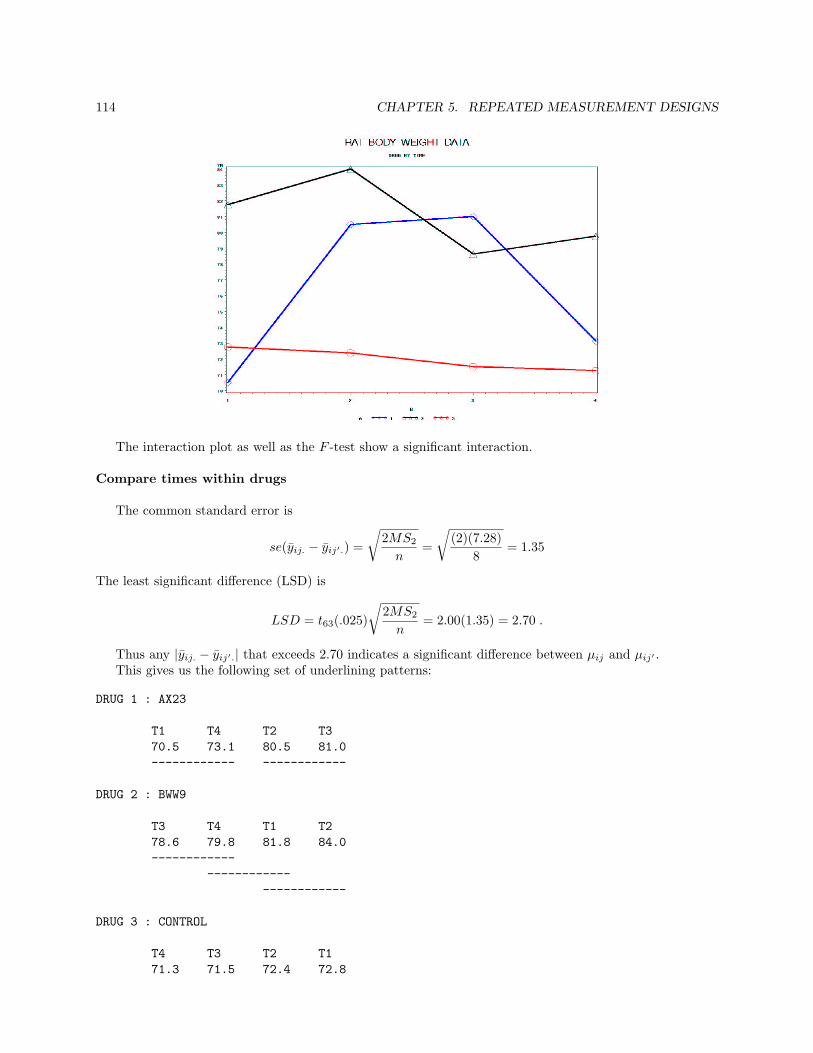
114 CHAPTER 5. REPEATED MEASUREMENT DESIGNS
The interaction plot as well as the F -test show a significant interaction.
Compare times within drugs
The common standard error is
se(yij. − yij′.) =
√2MS2
n=
√(2)(7.28)
8= 1.35
The least significant difference (LSD) is
LSD = t63(.025)
√2MS2
n= 2.00(1.35) = 2.70 .
Thus any |yij. − yij′.| that exceeds 2.70 indicates a significant difference between µij and µij′ .This gives us the following set of underlining patterns:
DRUG 1 : AX23
T1 T4 T2 T370.5 73.1 80.5 81.0------------ ------------
DRUG 2 : BWW9
T3 T4 T1 T278.6 79.8 81.8 84.0------------
------------------------
DRUG 3 : CONTROL
T4 T3 T2 T171.3 71.5 72.4 72.8

5.3. TWO-WAY REPEATED MEASUREMENT DESIGNS 115
----------------------------
Compare drugs within times
The common standard error is
se(yij. − yij′.) =
√2MS3
n=
√2(MS1 + (b− 1)MS2)
nb=
√2(110.5 + (3)(7.28))
(2)(8)= 2.876
with
df3 =a(n− 1)[MS1 + (b− 1)MS2]2
MS21 + (b− 1)MS2
2
=3(7)[110.5 + (3)(7.28)]2
(110.5)2 + (3)(7.28)2= 29.7 ≈ 30
The least significant difference (LSD) is
LSD = t30(.025)
√2MS3
n= 2.042(2.876) = 5.87 .
Thus any |yij. − yi′j.| that exceeds 5.87 indicates a significant difference between µij and µi′j .This gives us the following set of underlining patterns:
TIME 1AX23 CONTROL BWW970.5 72.8 81.75--------------
TIME 2CONTROL AX23 BWW972.4 80.5 84.0
------------
TIME 3CONTROL BWW9 AX2371.5 78.6 81.0
------------
TIME 4CONTROL AX23 BWW971.3 73.1 79.8----------------
The following example taken from Milliken and Johnson illustrates how SAS can be used to make com-parisons of means in the absence of a significant interaction.
Example
This experiment involved studying the effect of a dose of a drug on the growth of rats. The data set consistsof the growth of 15 rats, where 5 rats were randomly assigned to each of the 3 doses of the drug. The weightswere obtained each week for 4 weeks.

116 CHAPTER 5. REPEATED MEASUREMENT DESIGNS
WeekDose Rat 1 2 3 4
1 1 54 60 63 742 69 75 81 903 77 81 87 944 64 69 77 835 51 58 62 71
2 1 62 71 75 812 68 73 81 913 94 102 109 1124 81 90 95 1045 64 69 72 78
3 1 59 63 66 752 56 66 70 813 71 77 84 804 59 64 69 765 65 70 73 77
The SAS code and output are given below:
OPTIONS LS=80 PS=66 NODATE;DATA RM1;
DO A=1,2,3;DO S=1,2,3,4,5;
DO B = 1,2,3,4;INPUT Y @@;OUTPUT;
END;END;
END;CARDS;54 60 63 7469 75 81 9077 81 87 9464 69 77 8351 58 62 7162 71 75 8168 73 81 9194 102 109 11281 90 95 10464 69 72 7859 63 66 7556 66 70 8171 77 84 8059 64 69 7665 70 73 77;
PROC SORT DATA=RM1;BY A B S;
RUN;QUIT;
PROC MEANS MEAN NOPRINT;VAR Y;BY A B;OUTPUT OUT=OUTMEAN MEAN=YM;
RUN;QUIT;
GOPTIONS DISPLAY;PROC GPLOT DATA=OUTMEAN;
PLOT YM*B=A;SYMBOL1 V=DIAMOND L=1 I=JOIN CV=BLUE;SYMBOL2 V=TRIANGLE L=1 I=JOIN CV=BLACK;SYMBOL3 V=CIRCLE L=1 I=JOIN CV=ORANGE;

5.3. TWO-WAY REPEATED MEASUREMENT DESIGNS 117
TITLE3 ’DOSE BY TIME’;RUN;QUIT;
TITLE1 ’RAT BODY WEIGHT DATA’;PROC GLM DATA=RM1;
CLASS A B S;MODEL Y = A S(A) B A*B B*S(A);TEST H=A E=S(A);TEST H=B A*B E=B*S(A);LSMEANS A/PDIFF E=S(A);LSMEANS B/PDIFF E=B*S(A);
RUN;QUIT;
----------------------------------------------------------
Dependent Variable: Y
Sum ofSource DF Squares Mean Square F Value Pr > F
Model 59 10440.18333 176.95226 . .
Error 0 0.00000 .
Corrected Total 59 10440.18333
Source DF Type III SS Mean Square F Value Pr > F
A 2 2146.433333 1073.216667 . .S(A) 12 5405.500000 450.458333 . .B 3 2678.183333 892.727778 . .A*B 6 32.366667 5.394444 . .B*S(A) 36 177.700000 4.936111 . .
Tests of Hypotheses Using the Type III MS for S(A) as an Error Term
Source DF Type III SS Mean Square F Value Pr > F
A 2 2146.433333 1073.216667 2.38 0.1345
Tests of Hypotheses Using the Type III MS for B*S(A) as an Error Term
Source DF Type III SS Mean Square F Value Pr > F
B 3 2678.183333 892.727778 180.86 <.0001A*B 6 32.366667 5.394444 1.09 0.3854
The GLM ProcedureLeast Squares Means
Standard Errors and Probabilities Calculated Using the Type III MSfor S(A) as
an Error Term
LSMEANA Y LSMEAN Number
1 72.0000000 12 83.6000000 23 70.0500000 3
Least Squares Means for effect APr > |t| for H0: LSMean(i)=LSMean(j)
Dependent Variable: Y
i/j 1 2 3
1 0.1095 0.77642 0.1095 0.06643 0.7764 0.0664

118 CHAPTER 5. REPEATED MEASUREMENT DESIGNS
Least Squares MeansStandard Errors and Probabilities Calculated Using the Type III MS for B*S(A)
as an Error Term
LSMEANB Y LSMEAN Number
1 66.2666667 12 72.5333333 23 77.6000000 34 84.4666667 4
Least Squares Means for effect BPr > |t| for H0: LSMean(i)=LSMean(j)
Dependent Variable: Y
i/j 1 2 3 4
1 <.0001 <.0001 <.00012 <.0001 <.0001 <.00013 <.0001 <.0001 <.00014 <.0001 <.0001 <.0001
Since there is no significant interaction, the means of A and B can be compared at the highest level.Using the output from LSMEANS one obtains the following underlining patterns:
DOSES : D3 D1 D270.1 72.0 83.6--------------------
WEEKS : W1 W2 W3 W466.3 72.5 77.6 84.5
Two-Way RM Design : General Case
So far, we have considered the analysis of the classic two-way RM design under the assumption that the (S)condition is satisfied for each level of A. Here we consider the analysis of a two-way RM design where the(S) condition may not hold.

5.3. TWO-WAY REPEATED MEASUREMENT DESIGNS 119
The analysis strategy will be as follows:
1. Test the B main effect and the AB interaction effect using the G-G e-adjusted F -test.
2. Run a complete one-way ANOVA of the the levels of A within each level of B. That is, for level j ofB, we test H0 : µ1j = · · · = µaj and make multiple comparisons of means using the data
A1 · · · i · · · a
y1j1 · · · yij1 · · · yaj1
......
...y1jn1 · · · yijni
· · · yajna
3. Run a complete one-way RM analysis of the levels of B within each level of A using the G-G e-adjusted one-way RM F -tests followed by multiple comparisons of means. That is, for level i of A, wetest H0 : µi1 = · · · = µib using the data
BSubject 1 · · · j · · · a
1 yi11 · · · yij1 · · · yib1
......
......
k yi1k · · · yijk · · · yibk
......
......
ni yi1ni · · · yijni · · · yibni
Example
We will revisit the body weight of rats data considered above. The following SAS code is used to get thetests for B and AB effects.
OPTIONS LS=80 PS=66 NODATE;DATA RM3;INPUT A Y1 Y2 Y3 Y4;CARDS;1 54 60 63 741 69 75 81 901 77 81 87 941 64 69 77 831 51 58 62 712 62 71 75 812 68 73 81 912 94 102 109 1122 81 90 95 1042 64 69 72 783 59 63 66 753 56 66 70 813 71 77 84 803 59 64 69 763 65 70 73 77;
TITLE1 ’RAT BODY WEIGHT DATA : 2’;PROC GLM DATA=RM3;
CLASS A;MODEL Y1-Y4 = A;REPEATED B 4/ PRINTE;
RUN;QUIT;
--------------------------------------------------------------SELECTED OUTPUT--------------------------------------------------------------
RAT BODY WEIGHT DATA : 2 117

120 CHAPTER 5. REPEATED MEASUREMENT DESIGNS
Sphericity Tests
Mauchly’sVariables DF Criterion Chi-Square Pr > ChiSq
Transformed Variates 5 0.0459293 33.031436 <.0001Orthogonal Components 5 0.3345438 11.740697 0.0385
The GLM ProcedureRepeated Measures Analysis of Variance
Tests of Hypotheses for Between Subjects Effects
Source DF Type III SS Mean Square F Value Pr > F
A 2 2146.433333 1073.216667 2.38 0.1345Error 12 5405.500000 450.458333
RAT BODY WEIGHT DATA : 2 118
The GLM ProcedureRepeated Measures Analysis of Variance
Univariate Tests of Hypotheses for Within Subject Effects
Source DF Type III SS Mean Square F Value Pr > F
B 3 2678.183333 892.727778 180.86 <.0001B*A 6 32.366667 5.394444 1.09 0.3854Error(B) 36 177.700000 4.936111
Adj Pr > FSource G - G H - F
B <.0001 <.0001B*A 0.3811 0.3846Error(B)
Greenhouse-Geisser Epsilon 0.6058Huynh-Feldt Epsilon 0.8269
Using the G-G e-adjusted tests one observes that the AB interaction effect is not significant while the Bmain effect is significant both at α = .05. Mauchly’s test for the (S) condition is significant indicating thatthe analyses run earlier may not be the appropriate ones.
We now run one-way RM analyses of B within each level of A.
PROC SORT DATA=RM3;BY A;
RUN;QUIT;
PROC GLM DATA=RM3;MODEL Y1-Y4=/NOUNI;REPEATED B 4/PRINTE;BY A;
RUN;QUIT;
-----------------------------------------------------------------SELECTED OUTPUT-----------------------------------------------------------------
RAT BODY WEIGHT DATA : 2 119
------------------------------------- A=1 --------------------------------------
Sphericity Tests
Mauchly’sVariables DF Criterion Chi-Square Pr > ChiSq
Transformed Variates 5 0.1626147 4.9445682 0.4227Orthogonal Components 5 0.27398 3.5244612 0.6197

5.3. TWO-WAY REPEATED MEASUREMENT DESIGNS 121
The GLM ProcedureRepeated Measures Analysis of Variance
Univariate Tests of Hypotheses for Within Subject Effects
Source DF Type III SS Mean Square F Value Pr > F
B 3 1023.600000 341.200000 284.33 <.0001Error(B) 12 14.400000 1.200000
Adj Pr > FSource G - G H - F
B <.0001 <.0001Error(B)
Greenhouse-Geisser Epsilon 0.6286Huynh-Feldt Epsilon 1.1713
------------------------------------- A=2 --------------------------------------
Sphericity Tests
Mauchly’sVariables DF Criterion Chi-Square Pr > ChiSq
Transformed Variates 5 0.0706227 7.2149884 0.2051Orthogonal Components 5 0.3812237 2.6252267 0.7575
The GLM ProcedureRepeated Measures Analysis of Variance
Univariate Tests of Hypotheses for Within Subject Effects
Source DF Type III SS Mean Square F Value Pr > F
B 3 1014.000000 338.000000 78.00 <.0001Error(B) 12 52.000000 4.333333
Adj Pr > FSource G - G H - F
B <.0001 <.0001Error(B)
Greenhouse-Geisser Epsilon 0.6370Huynh-Feldt Epsilon 1.2055
------------------------------------- A=3 --------------------------------------
Sphericity Tests
Mauchly’sVariables DF Criterion Chi-Square Pr > ChiSq
Transformed Variates 5 0.0055188 14.15447 0.0147Orthogonal Components 5 0.052686 8.0126045 0.1555
The GLM ProcedureRepeated Measures Analysis of Variance
Univariate Tests of Hypotheses for Within Subject Effects
Source DF Type III SS Mean Square F Value Pr > F
B 3 672.9500000 224.3166667 24.19 <.0001Error(B) 12 111.3000000 9.2750000
Adj Pr > FSource G - G H - F
B 0.0021 0.0004Error(B)
Greenhouse-Geisser Epsilon 0.4800

122 CHAPTER 5. REPEATED MEASUREMENT DESIGNS
Huynh-Feldt Epsilon 0.6772
Sphericity is satisfied in all the three cases. The repeated factor B is also significant in all the cases.Thus, we may compare the means of B using the MSE as a denominator. In the situation where the (S)condition is not satisfied in one or more of the groups, one uses Welch t-tests, as shown in the last exampleof Section 5.2, to compare the means of B in the particular group which does not satisfy the (S) condition.
The following SAS code re-creates the data as A, B, S, Y columns and runs:
• the one-way ANOVA for the factor A within each level of B;
• comparisons of the A means for each level of B; and
• comparisons of the B means within each level of A.
DATA RM4;SET RM3;ARRAY Z Y1-Y4;DO B=1,2,3,4;
S = _N_;Y = Z(B);OUTPUT;
END;DROP Y1-Y4;
RUN;QUIT;
PROC SORT DATA=RM4;BY B;
RUN;QUIT;
PROC GLM DATA=RM4;CLASS A;MODEL Y=A;LSMEANS A/PDIFF;BY B;
RUN;QUIT;
PROC SORT DATA=RM4;BY A;
RUN;QUIT;
PROC GLM DATA=RM4;CLASS B S;MODEL Y=B S;LSMEANS B/ PDIFF;BY A;
RUN;QUIT;
-------------------------------------------------------------SELECTED OUTPUT-------------------------------------------------------------
RAT BODY WEIGHT DATA : 2 140
------------------------------------- B=1 --------------------------------------The GLM Procedure
Dependent Variable: Y
Sum ofSource DF Squares Mean Square F Value Pr > F
Model 2 428.133333 214.066667 1.93 0.1876Error 12 1330.800000 110.900000

5.3. TWO-WAY REPEATED MEASUREMENT DESIGNS 123
Corrected Total 14 1758.933333
Source DF Type III SS Mean Square F Value Pr > F
A 2 428.1333333 214.0666667 1.93 0.1876
The GLM ProcedureLeast Squares Means
LSMEANA Y LSMEAN Number
1 63.0000000 12 73.8000000 23 62.0000000 3
Least Squares Means for effect APr > |t| for H0: LSMean(i)=LSMean(j)
Dependent Variable: Y
i/j 1 2 3
1 0.1309 0.88312 0.1309 0.10183 0.8831 0.1018
------------------------------------- B=2 --------------------------------------The GLM Procedure
Dependent Variable: Y
Sum ofSource DF Squares Mean Square F Value Pr > F
Model 2 538.533333 269.266667 2.41 0.1319Error 12 1341.200000 111.766667
Corrected Total 14 1879.733333
Source DF Type III SS Mean Square F Value Pr > F
A 2 538.5333333 269.2666667 2.41 0.1319
The GLM ProcedureLeast Squares Means
LSMEANA Y LSMEAN Number
1 68.6000000 12 81.0000000 23 68.0000000 3
Least Squares Means for effect APr > |t| for H0: LSMean(i)=LSMean(j)
Dependent Variable: Y
i/j 1 2 3
1 0.0884 0.93002 0.0884 0.07573 0.9300 0.0757
------------------------------------- B=3 --------------------------------------The GLM Procedure
Dependent Variable: Y
Sum ofSource DF Squares Mean Square F Value Pr > F

124 CHAPTER 5. REPEATED MEASUREMENT DESIGNS
Model 2 587.200000 293.600000 2.15 0.1589Error 12 1636.400000 136.366667
Corrected Total 14 2223.600000
Source DF Type III SS Mean Square F Value Pr > F
A 2 587.2000000 293.6000000 2.15 0.1589
The GLM ProcedureLeast Squares Means
LSMEANA Y LSMEAN Number
1 74.0000000 12 86.4000000 23 72.4000000 3
Least Squares Means for effect APr > |t| for H0: LSMean(i)=LSMean(j)
Dependent Variable: Y
i/j 1 2 3
1 0.1190 0.83212 0.1190 0.08243 0.8321 0.0824
------------------------------------- B=4 --------------------------------------The GLM Procedure
Dependent Variable: Y
Sum ofSource DF Squares Mean Square F Value Pr > F
Model 2 624.933333 312.466667 2.94 0.0913Error 12 1274.800000 106.233333
Corrected Total 14 1899.733333
The GLM ProcedureLeast Squares Means
LSMEANA Y LSMEAN Number
1 82.4000000 12 93.2000000 23 77.8000000 3
Least Squares Means for effect APr > |t| for H0: LSMean(i)=LSMean(j)
Dependent Variable: Y
i/j 1 2 3
1 0.1235 0.49392 0.1235 0.03593 0.4939 0.0359
RAT BODY WEIGHT DATA : 2 152
------------------------------------- A=1 --------------------------------------The GLM Procedure
Dependent Variable: Y
Sum of

5.3. TWO-WAY REPEATED MEASUREMENT DESIGNS 125
Source DF Squares Mean Square F Value Pr > F
Model 7 2733.600000 390.514286 325.43 <.0001Error 12 14.400000 1.200000
Corrected Total 19 2748.000000
Source DF Type III SS Mean Square F Value Pr > F
B 3 1023.600000 341.200000 284.33 <.0001S 4 1710.000000 427.500000 356.25 <.0001
The GLM ProcedureLeast Squares Means
LSMEANB Y LSMEAN Number
1 63.0000000 12 68.6000000 23 74.0000000 34 82.4000000 4
Least Squares Means for effect BPr > |t| for H0: LSMean(i)=LSMean(j)
Dependent Variable: Y
i/j 1 2 3 4
1 <.0001 <.0001 <.00012 <.0001 <.0001 <.00013 <.0001 <.0001 <.00014 <.0001 <.0001 <.0001
------------------------------------- A=2 --------------------------------------The GLM Procedure
Dependent Variable: Y
Sum ofSource DF Squares Mean Square F Value Pr > F
Model 7 4326.800000 618.114286 142.64 <.0001Error 12 52.000000 4.333333
Corrected Total 19 4378.800000
Source DF Type III SS Mean Square F Value Pr > F
B 3 1014.000000 338.000000 78.00 <.0001S 4 3312.800000 828.200000 191.12 <.0001
The GLM ProcedureLeast Squares Means
LSMEANB Y LSMEAN Number
1 73.8000000 12 81.0000000 23 86.4000000 34 93.2000000 4
Least Squares Means for effect BPr > |t| for H0: LSMean(i)=LSMean(j)
Dependent Variable: Y
i/j 1 2 3 4
1 0.0001 <.0001 <.00012 0.0001 0.0015 <.00013 <.0001 0.0015 0.00024 <.0001 <.0001 0.0002

126 CHAPTER 5. REPEATED MEASUREMENT DESIGNS
------------------------------------- A=3 --------------------------------------The GLM Procedure
Dependent Variable: Y
Sum ofSource DF Squares Mean Square F Value Pr > F
Model 7 1055.650000 150.807143 16.26 <.0001Error 12 111.300000 9.275000
Corrected Total 19 1166.950000
Source DF Type III SS Mean Square F Value Pr > F
B 3 672.9500000 224.3166667 24.19 <.0001S 4 382.7000000 95.6750000 10.32 0.0007
The GLM ProcedureLeast Squares Means
LSMEANB Y LSMEAN Number
1 62.0000000 12 68.0000000 23 72.4000000 34 77.8000000 4
Least Squares Means for effect BPr > |t| for H0: LSMean(i)=LSMean(j)
Dependent Variable: Y
i/j 1 2 3 4
1 0.0089 0.0002 <.00012 0.0089 0.0414 0.00033 0.0002 0.0414 0.01594 <.0001 0.0003 0.0159
Using underlining to summarize the results
Group(A) B levels--------- --------------
1 B1 B2 B3 B42 B1 B2 B3 B43 B1 B2 B3 B4
Treatment(B) A levels------------ ------------------
1 A3 A1 A2------------------
2 A3 A1 A2------------------
3 A3 A1 A2------------------
4 A3 A1 A2----------
----------

5.3. TWO-WAY REPEATED MEASUREMENT DESIGNS 127

128 CHAPTER 5. REPEATED MEASUREMENT DESIGNS

Chapter 6
More on Repeated MeasurementDesigns
In this chapter we will further investigate one- and two-way repeated measurement designs. Since RM designsusually involve a time factor, one may be interested in the pattern of the response variable over time. Thus,we shall consider trend analysis in one- and two-way RM designs as our first section. Later sections considerspecial cases of the two-way RM design.
6.1 Trend Analyses in One- and Two-way RM Designs
6.1.1 Regression Components of the Between Treatment SS (SSB)
Often the treatments in an experiment consist of levels of a quantitative variable. For instance, in a one-wayCRD model, the treatments may be several dosages of the same drug. One is usually interested in developingan equation for a curve that describes the dose-response relationship. This may be used to find the optimaldosage level. To this end we want to consider applications of regression procedures within the ANOVAframework.
As an illustration, consider the fabric strength experiment considered in Chapter 1. The treatmentconsists of five different levels of cotton percentages and the response is the strength of the fabric produced.Each percentage of cotton is randomly assigned to five randomly selected experimental units. This is theusual CRD framework that is represented by the model
yij = µ + τi + εij , i = 1, · · · , 5, j = 1, · · · , 5 ,
where our interest lies in testing
H0 : τ1 = τ2 = · · · = τ5 = 0HA : τi 6= 0 for at least one i
which is tested using F0 = MSB/MSW .We can get more insight into the nature of the relationship of the response, y, and the levels of the
treatment variable, x, if we consider a regression type relationship between x and y; i.e
y = f(x) + ε
For example, one may consider the simple linear regression model
y = β0 + β1x + ε
and testH0 : β1 = 0
to determine if the response is linearly related to the levels of the treatment.
129

130 CHAPTER 6. MORE ON REPEATED MEASUREMENT DESIGNS
Partitioning SSB
The variability in the response that is explained by the treatment may now be partitioned into that due tothe linear regression and that due to the remainder that cannot be explained by the regression model. Thus,
SSB = SSR + SSL
where SSR is the sum of squares due to the linear regression and SSL is the sum of squares due to lack offit (i.e failure of the linear regression to describe the relationship between x and y).
The ANOVA table for the CRD is
Source df SS MS F0
Between k − 1 SSB MSB F0 = MSB/MSW
Linear Regression 1 SSR MSR FR = MSR/MSW
Lack of Fit k − 2 SSL MSL FL = MSL/MSW
Within (Error) n− k SSW MSW
Total n− 1 SST
One may obtain SSR by fitting an ordinary linear regression model of y on x. This, however, seemsto be the hard way as the F values may have to be computed by hand. An easier way is to find a set ofcoefficients to define a contrast among the treatment means. To use this approach we may define contrastsusing the deviations of the treatment levels from the treatment mean as our contrast coefficients. Withoutloss of generality, assume that we have a balanced CRD model where r represents the number of replicationsper treatment level. Assume also that we have k treatment levels. Then
φR =k∑
i=1
(xi − x)µi
is a contrast (∑k
i=1(xi − x) = 0) whose estimator is
φR =k∑
i=1
(xi − x)yi
From φR we get
SSR =rφ2
R∑ki=1(xi − x)2
andSSL = SSB − SSR .
The F ratios in the above ANOVA table are used to test the following hypotheses:
1. F0 is a test statistic for testingH0 : τ1 = · · · = τk = 0 ,
the hypothesis that all the treatment means are the same against the alternative that at least two aredifferent.
2. FR is a test statistic for testingH0 : β1 = 0 ,
the hypothesis that there is no linear relationship between the response and the levels of the treatmentagainst the alternative that there is a significant linear relationship.
3. FL is the test statistic for testingH0 : E(y) = β0 + β1x ,
the hypothesis that the simple linear regression model describes the data against the alternative thata simple linear model is not sufficient.

6.1. TREND ANALYSES IN ONE- AND TWO-WAY RM DESIGNS 131
Orthogonal Polynomials
The fitting of curves within the ANOVA framework can be greatly simplified if
1. the design is balanced; and,
2. the treatment levels are equally spaced.
In such a case we may replace (xi − x) by a simple set of multipliers known as orthogonal polynomialcoefficients. These coefficients are extensively tabulated but we will use Proc IML in SAS to generatethem. These coefficients enable us to partition SSB into orthogonal linear, quadratic, cubic, quartic, etc.components each with one degree of freedom. This means that SSB can be completely decomposed usinga polynomial of degree k − 1 with no lack of fit term. The usual procedure is to fit successive terms of thepolynomial starting with the linear term until lack of fit becomes non-significant. This is very widely usedin practice even though it sometimes entail premature stopping.
Assume that cij , i = 1, . . . , k−1, j = 1, . . . , k be the ith order polynomial coefficient for the jth treatmentlevel. Then
Li =k∑
j=1
cij yj
is the contrast of means associated with the ith order term of the polynomial, and
S2i =
rL2i∑k
j=1 c2ij
is the 1 df sum of squares associated with the ith term.Proc IML in SAS may be used to generate orthogonal polynomial coefficients. For instance, consider a
case where the treatment has k = 4 levels, say, 10, 20, 30, 40, and 50. The orthogonal polynomial coefficientsfor all four terms of the polynomial
y = β0 + β1x + β11x2 + β111x
3 + β1111x4
are computed as
proc iml;x={10 20 30 40 50};xp=orpol(x,4);print xp;run;quit;
The output is
0.4472136 -0.632456 0.5345225 -0.316228 0.11952290.4472136 -0.316228 -0.267261 0.6324555 -0.4780910.4472136 3.588E-18 -0.534522 1.86E-16 0.71713720.4472136 0.3162278 -0.267261 -0.632456 -0.4780910.4472136 0.6324555 0.5345225 0.3162278 0.1195229
The first column represents the intercept term.Note that in SAS the treatment levels need not be equally spaced. For example
proc iml;x={0 25 75 100};xp=orpol(x,3);print xp;run;quit;

132 CHAPTER 6. MORE ON REPEATED MEASUREMENT DESIGNS
gives
0.5 -0.632456 0.5 -0.3162280.5 -0.316228 -0.5 0.63245550.5 0.3162278 -0.5 -0.6324560.5 0.6324555 0.5 0.3162278
The following code and associated plot show how the contrast coefficients are related to the polynomialterms.
Title1 "Orthogonal Polynomials";Title2 "5 Equallyspaced Levels";Data Five;Length Trend $9;Input Trend @;Do X=4,5,6,7,8;Input Coef @;Output;End;Datalines;linear -0.632456 -0.316228 1.969E-17 0.3162278 0.6324555quadratic 0.5345225 -0.267261 -0.534522 -0.267261 0.5345225cubic -0.316228 0.6324555 6.501E-17 -0.632456 0.3162278quartic 0.1195229 -0.478091 0.7171372 -0.478091 0.1195229;
proc print;run;quit;
Proc GPlot Data=Five;Plot Coef*X=Trend / VAxis=Axis1;Axis1 Label=(A=90 "Coefficient") Order=(-1 To 1 By .1);Symbol1 C=Black V=Triangle L=1 I=Spline;Symbol2 C=Black V=Square L=1 I=Spline;Symbol3 C=Black V=Diamond L=1 I=Spline;Symbol4 C=Black V=Circle L=1 I=Spline;Run;Quit;

6.1. TREND ANALYSES IN ONE- AND TWO-WAY RM DESIGNS 133
EXAMPLE: An experiment was conducted to determine the effect of storage temperature on potency ofan antibiotic. Fifteen samples of the antibiotic were obtained and three samples, selected at random, werestored at each of five temperatures. After 30 days of storage the samples were tested for potency. The resultsare given below:
Temperature10◦ 30◦ 50◦ 70◦ 90◦
62 26 16 10 1355 36 15 11 1157 31 23 18 9
The contrast coefficients in the following code were generated using Proc IML in SAS.
data potency;input temp pot @@;cards;
10 62 10 55 10 5730 26 30 36 30 3150 16 50 15 50 2370 10 70 11 70 1890 13 90 11 90 9
;
proc glm;class temp;model pot = temp;contrast ’linear’ temp -0.632456 -0.316228 1.969E-17 0.3162278 0.6324555;contrast ’quadratic’ temp 0.5345225 -0.267261 -0.534522 -0.267261 0.5345225;contrast ’cubic’ temp -0.316228 0.6324555 6.501E-17 -0.632456 0.3162278;contrast ’quartic’ temp 0.1195229 -0.478091 0.7171372 -0.478091 0.1195229;
run; quit;
proc glm;model pot=temp temp*temp;output out=quadmod p=p;
run;

134 CHAPTER 6. MORE ON REPEATED MEASUREMENT DESIGNS
quit;
proc gplot data=quadmod;plot p*temp/ vaxis=axis1;axis1 label=(A=90 "Y");symbol1 c=black V=square L=1 I=spline;
run;quit;
The following is the ANOVA table that is produced by SAS:
Source DF Type I SS Mean Square F Value Pr > F
temp 4 4520.400000 1130.100000 70.63 <.0001linear 1 3763.199609 3763.199609 235.20 <.0001quadratic 1 720.859329 720.859329 45.05 <.0001cubic 1 36.300220 36.300220 2.27 0.1629quartic 1 0.042866 0.042866 0.00 0.9597
Error 10 160.000000 16.000000Corrected Total 14 4680.400000
Over the 30 day storage period used in this study temperature had a highly significant effect on thepotency of the antibiotic (P < .0001). The linear and quadratic terms are the only significant trend com-ponents. So we will fit a quadratic model using SAS’ Proc GLM. Over the temperature range 10◦ to 90◦,potency may be described by the equation
y = 71.80− 1.60x + .01x2
where y is the expected potency and x is the 30-day storage temperature.The issue of trend analysis involving more than one independent variable, and response surface method-
ology in general, will be investigated in a greater detail in a later chapter.
6.1.2 RM Designs
Consider those cases where the within subject factor, denoted by B hereafter, involves b time measurementsat times t1 < t2 < . . . < tb. Let φ =
∑bi=1 cjµ.j or φ =
∑bi=1 cjµij be a polynomial contrast of the main B
means or the simple B means specific to Group i, respectively. Let φ1, φ2, . . . , φb−1 be the b− 1 orthogonalpolynomial contrasts, where φi is degree i.
One may use the POLYNOMIAL transformation option of SAS to obtain trend analysis. In the followingwe will consider two examples: one- and two-way RM designs.
The following is due to Michael Stoline, Personal Communication.
Example : One-way RM Design
In a small pilot clinical trial dose-response drug study, a pharmaceutical company research team is concernedwith the quickness that a new drug can sedate a person so that they can go to sleep. A sample b = 8 peopleis selected from a population of insomniacs, who have no medically-diagnosed physical or mental disease orsymptoms, which may cause or explain the insomnia. A Likert scale is used to determine ease in going tosleep. The scale used in the study is:

6.1. TREND ANALYSES IN ONE- AND TWO-WAY RM DESIGNS 135
Scale Time to go to sleep (in minutes)1 < 102 10− 203 20− 404 > 40
Each of the subjects in the insomniac population has chronic sleep difficulties, and each consistently scoresa value of 4 in their daily evaluation of time required to go to sleep, using the above instrument. A standarddosage of the new drug is administered daily to each of the eight subjects under the care of a physician.Sleep difficulty, in the above Likert scale, is measured for each patient after one, two, four, and eight weeks.The goal of the study is to assess the relationship of the ease of going to sleep as a function of the length oftime under medication. In particular we would like to test the significance of the linear quadratic and cubicorthogonal trend components of sleep difficulty as a function of time. The data are given below:
Sleep Difficulty ScaleSubject 1 week 2 weeks 4 weeks 8 weeks
1 4 2 2 12 2 2 1 13 2 2 2 24 4 3 3 25 3 2 1 16 3 1 2 17 1 1 2 18 2 2 1 2
The following SAS code is used to perform orthogonal trend analysis.
DATA RM1;
INPUT B1 B2 B3 B4;
CARDS;
4 2 2 1
2 2 1 1
2 2 2 2
4 3 3 2
3 2 1 1
3 1 2 1
1 1 2 1
2 2 1 2
;
TITLE ’ONE-WAY RM TREND’; PROC GLM DATA=RM1;
MODEL B1-B4 = / NOUNI;
REPEATED TIME 4 (1 2 4 8) POLYNOMIAL / PRINTM SUMMARY;
RUN; QUIT;
The related output is
-------------------------------------------------------------------------------
TIME_N represents the nth degree polynomial contrast for TIME
M Matrix Describing Transformed Variables
B1 B2 B3 B4
TIME_1 -.5128776445 -.3263766829 0.0466252404 0.7926290870
TIME_2 0.5296271413 -.1059254283 -.7679593549 0.3442576419
TIME_3 -.4543694674 0.7951465679 -.3975732840 0.0567961834
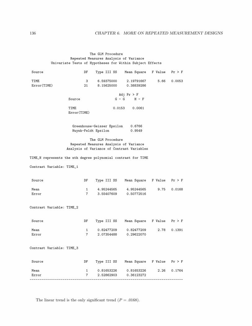
136 CHAPTER 6. MORE ON REPEATED MEASUREMENT DESIGNS
The GLM Procedure
Repeated Measures Analysis of Variance
Univariate Tests of Hypotheses for Within Subject Effects
Source DF Type III SS Mean Square F Value Pr > F
TIME 3 6.59375000 2.19791667 5.66 0.0053
Error(TIME) 21 8.15625000 0.38839286
Adj Pr > F
Source G - G H - F
TIME 0.0153 0.0061
Error(TIME)
Greenhouse-Geisser Epsilon 0.6766
Huynh-Feldt Epsilon 0.9549
The GLM Procedure
Repeated Measures Analysis of Variance
Analysis of Variance of Contrast Variables
TIME_N represents the nth degree polynomial contrast for TIME
Contrast Variable: TIME_1
Source DF Type III SS Mean Square F Value Pr > F
Mean 1 4.95244565 4.95244565 9.75 0.0168
Error 7 3.55407609 0.50772516
Contrast Variable: TIME_2
Source DF Type III SS Mean Square F Value Pr > F
Mean 1 0.82477209 0.82477209 2.78 0.1391
Error 7 2.07354488 0.29622070
Contrast Variable: TIME_3
Source DF Type III SS Mean Square F Value Pr > F
Mean 1 0.81653226 0.81653226 2.26 0.1764
Error 7 2.52862903 0.36123272
-------------------------------------------------------------------------------
The linear trend is the only significant trend (P = .0168).
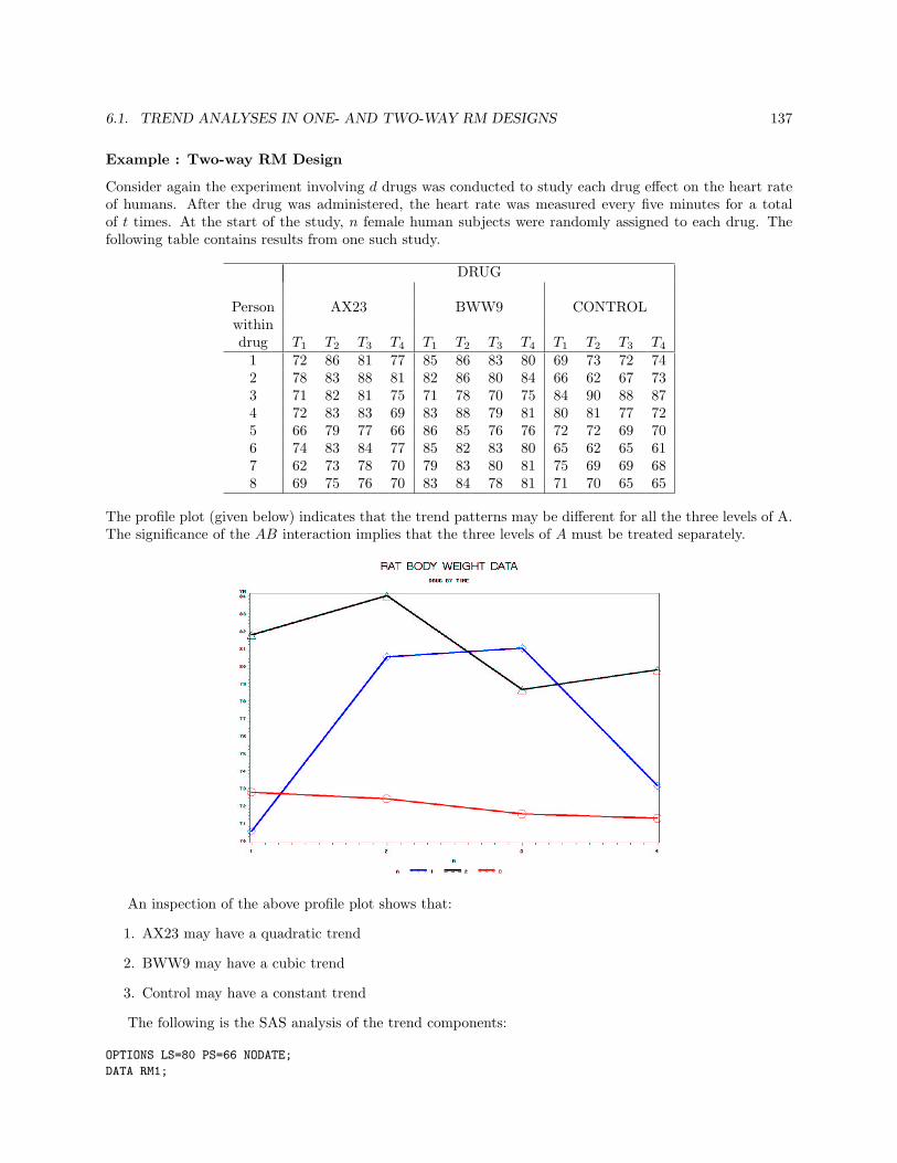
6.1. TREND ANALYSES IN ONE- AND TWO-WAY RM DESIGNS 137
Example : Two-way RM Design
Consider again the experiment involving d drugs was conducted to study each drug effect on the heart rateof humans. After the drug was administered, the heart rate was measured every five minutes for a totalof t times. At the start of the study, n female human subjects were randomly assigned to each drug. Thefollowing table contains results from one such study.
DRUG
Person AX23 BWW9 CONTROLwithindrug T1 T2 T3 T4 T1 T2 T3 T4 T1 T2 T3 T4
1 72 86 81 77 85 86 83 80 69 73 72 742 78 83 88 81 82 86 80 84 66 62 67 733 71 82 81 75 71 78 70 75 84 90 88 874 72 83 83 69 83 88 79 81 80 81 77 725 66 79 77 66 86 85 76 76 72 72 69 706 74 83 84 77 85 82 83 80 65 62 65 617 62 73 78 70 79 83 80 81 75 69 69 688 69 75 76 70 83 84 78 81 71 70 65 65
The profile plot (given below) indicates that the trend patterns may be different for all the three levels of A.The significance of the AB interaction implies that the three levels of A must be treated separately.
An inspection of the above profile plot shows that:
1. AX23 may have a quadratic trend
2. BWW9 may have a cubic trend
3. Control may have a constant trend
The following is the SAS analysis of the trend components:
OPTIONS LS=80 PS=66 NODATE;
DATA RM1;

138 CHAPTER 6. MORE ON REPEATED MEASUREMENT DESIGNS
INPUT A Y1 Y2 Y3 Y4 @@;
CARDS;
1 72 86 81 77 2 85 86 83 80 3 69 73 72 74
1 78 83 88 81 2 82 86 80 84 3 66 62 67 73
1 71 82 81 75 2 71 78 70 75 3 84 90 88 87
1 72 83 83 69 2 83 88 79 81 3 80 81 77 72
1 66 79 77 66 2 86 85 76 76 3 72 72 69 70
1 74 83 84 77 2 85 82 83 80 3 65 62 65 61
1 62 73 78 70 2 79 83 80 81 3 75 69 69 68
1 69 75 76 70 2 83 84 78 81 3 71 70 65 65
;
TITLE1 ’HEART RATE DATA : TREND’;
PROC SORT DATA=RM1;
BY A;
RUN;
QUIT;
PROC GLM DATA=RM1;
CLASS A;
MODEL Y1-Y4 = /NOUNI;
REPEATED B 4 POLYNOMIAL/ PRINTM SUMMARY;
BY A;
RUN;
QUIT;
Selected output
------------------------------------- A=1 --------------------------------------
B_N represents the nth degree polynomial contrast for B
Contrast Variable: B_1
Source DF Type III SS Mean Square F Value Pr > F
Mean 1 28.05625000 28.05625000 4.37 0.0748
Error 7 44.89375000 6.41339286
Contrast Variable: B_2
Source DF Type III SS Mean Square F Value Pr > F
Mean 1 639.0312500 639.0312500 109.86 <.0001
Error 7 40.7187500 5.8169643
Contrast Variable: B_3
Source DF Type III SS Mean Square F Value Pr > F
Mean 1 0.50625000 0.50625000 0.10 0.7564
Error 7 34.04375000 4.86339286
------------------------------------- A=2 --------------------------------------
Contrast Variable: B_1
Source DF Type III SS Mean Square F Value Pr > F

6.1. TREND ANALYSES IN ONE- AND TWO-WAY RM DESIGNS 139
Mean 1 51.75625000 51.75625000 5.18 0.0570
Error 7 69.99375000 9.99910714
Contrast Variable: B_2
Source DF Type III SS Mean Square F Value Pr > F
Mean 1 2.53125000 2.53125000 2.16 0.1855
Error 7 8.21875000 1.17410714
Contrast Variable: B_3
Source DF Type III SS Mean Square F Value Pr > F
Mean 1 79.80625000 79.80625000 11.65 0.0112
Error 7 47.94375000 6.84910714
------------------------------------- A=3 --------------------------------------
Contrast Variable: B_1
Source DF Type III SS Mean Square F Value Pr > F
Mean 1 11.5562500 11.5562500 0.62 0.4566
Error 7 130.2937500 18.6133929
Contrast Variable: B_2
Source DF Type III SS Mean Square F Value Pr > F
Mean 1 0.03125000 0.03125000 0.00 0.9511
Error 7 54.21875000 7.74553571
Contrast Variable: B_3
Source DF Type III SS Mean Square F Value Pr > F
Mean 1 0.50625000 0.50625000 0.13 0.7332
Error 7 28.14375000 4.02053571
The results match our prior expectations:
1. AX23 - quadratic
2. BWW9 - cubic
3. Control - No trend

140 CHAPTER 6. MORE ON REPEATED MEASUREMENT DESIGNS
6.2 The Split-Plot Design
In some multi-factor designs that involve blocking, we may not be able to completely randomize the orderof runs within each block. This results in a design known as the split-plot design which is a generalization ofthe RCBD (or a subset of the classic two-way RM design, as we shall see later).
We shall only consider the simplest split-plot design that involves two factors and an incomplete block.There are two sizes of experimental units: whole plots are the larger units and subplots or split-plots arethe smaller units. The levels of one factor are assigned at random to large experimental units within blocksof such units. The large units are then divided into smaller units, and the levels of the second factor areassigned at random to the small units within the larger units.
An agronomist may be interested in the effect of tillage treatments and fertilizers on yield. Tillagemachinery requires large plots while fertilizers can be applied to small plots. One such experiment considersthree methods of seedbed preparation (S1, S2, S3) as a whole-plot factor and four rates of nitrogen fertilizerapplied by hand (N0, N1, N2, N3) as the subplot factor. The analysis is divided into two parts: whole plotand subplot. The three methods of land preparation are applied to the whole plots in random order. Theneach plot is divided into four subplots and the four different fertilizers are applied in random order.
Whole PlotsS3 S1 S2 S1 S3 S2
N3 N2 N0 N3 N0 N1
N2 N3 N3 N2 N1 N0
N1 N0 N2 N0 N3 N3
N0 N1 N1 N1 N2 N2
The statistical model associated with the split-plot design is
yijk = µ + τi + εij + βj + (τβ)ij + eijk,
i = 1, · · · , a
j = 1, · · · , b
k = 1, · · · , r
where µ + τi + εij is the whole plot part of the model and βj + (τβ)ij + eijk is the subplot part. Here a isthe number of levels of the whole plot factor, b is the number of levels of the subplot factor, and r is thenumber of times a whole plot factor is repeated. Notice that our design restricts the number of whole plotsto be a multiple of a. We may have unequal number of repetitions of the whole plot factor if the number ofwhole plots is not a multiple of a.
The ANOVA table for this split-plot design is
Source of Variation dfWhole Plot Analysis
A a− 1Error(Whole Plot) a(r − 1)
Subplot AnalysisB b− 1AB (a− 1)(b− 1)Error(Subplot) a(b− 1)(r − 1)
Notice that the ANOVA table looks like a two-way RM design ANOVA where the whole plot analysishere corresponds to the between subject analysis of the RM design and the subplot analysis corresponds tothe within subject analysis of the RM design.
The following example is taken from Milliken and Johnson.

6.2. THE SPLIT-PLOT DESIGN 141
Example
The following data are taken from an experiment where the amount of dry matter was measured on wheatplants grown in different levels of moisture and different amounts of fertilizer. There where 48 different peatpots and 12 plastic trays; 4 pots could be put into each tray. The moisture treatment consisted of adding10, 20, 30, or 40 ml of water per pot per day to the tray, where the water was absorbed by the peat pots.The levels of moisture were randomly assigned to the trays. The levels of fertilizer were 2, 4, 6, or 8 mg perpot. The four levels of fertilizer were randomly assigned to the four pots in each tray so that each fertilizeroccurred once in each tray. The wheat seeds were planted in each pot and after 30 days the dry matter ofeach pot was measured.
Level of Level of FertilizerMoisture Tray 2 4 6 8
1 3.3458 4.3170 4.5572 5.879410 2 4.0444 4.1413 6.5173 7.3776
3 1.97584 3.8397 4.4730 5.11804 5.0490 7.9419 10.7697 13.5168
20 5 5.91310 8.5129 10.3934 13.91576 6.95113 7.0265 10.9334 15.27507 6.56933 10.7348 12.2626 15.7133
30 8 8.29741 8.9081 13.4373 14.95759 5.27853 8.6654 11.1372 15.633210 6.8393 9.0842 10.3654 12.5144
40 11 6.4997 6.0702 10.7486 12.503412 4.0482 3.8376 9.4367 10.2811
The data was placed in a file called ”split2.dat” in the following format:
moist fert tray yield10 2 1 3.345810 2 2 4.044410 2 3 1.9758410 4 1 4.317010 4 2 4.141310 4 3 3.8397
...
40 8 10 12.514440 8 11 12.503440 8 12 10.2811
The following SAS code uses two ways (PROC GLM and PROC MIXED) to perform the split-plotanalysis.
OPTIONS LINESIZE=80 PAGESIZE=37; /* SPLIT PLOT MJ 24.2 */DATA EXPT;
INFILE ’C:\ASH\S7010\SAS\SPLIT2.DAT’ FIRSTOBS=2;INPUT MOIST FERT TRAY YIELD;
RUN;QUIT;
PROC GLM; /* SPLIT PLOT USING GLM */CLASS TRAY FERT MOIST;MODEL YIELD = MOIST TRAY(MOIST) FERT MOIST*FERT / SS1;RANDOM TRAY(MOIST) / TEST; /* TESTS USING RANDOM STATEMENT */TEST H = MOIST E = TRAY(MOIST); /* TESTS USING TEST STATEMENT */MEANS MOIST / LSD E = TRAY(MOIST); /* MEANS OK FOR BALANCED DATA */

142 CHAPTER 6. MORE ON REPEATED MEASUREMENT DESIGNS
MEANS FERT / LSD;LSMEANS MOIST*FERT / PDIFF STDERR OUT=LSM; /* SAVE LS MEANS DATASET */
RUN;QUIT;
PROC PLOT DATA=LSM; /* INTERACTION PLOTS FROM GLM */PLOT LSMEAN*FERT=MOIST;PLOT LSMEAN*MOIST=FERT;
RUN;QUIT;
PROC MIXED DATA=EXPT; /* SPLIT PLOT USING MIXED */CLASS TRAY FERT MOIST;MODEL YIELD = MOIST | FERT;RANDOM TRAY(MOIST);
RUN;QUIT;
----------------------------------------------------------------Sum of
Source DF Squares Mean Square F Value Pr > F
Model 23 631.5513647 27.4587550 36.51 <.0001Error 24 18.0513405 0.7521392
Corrected Total 47 649.6027051
Source DF Type I SS Mean Square F Value Pr > F
moist 3 269.1895496 89.7298499 119.30 <.0001tray(moist) 8 27.2515182 3.4064398 4.53 0.0019fert 3 297.0540027 99.0180009 131.65 <.0001fert*moist 9 38.0562942 4.2284771 5.62 0.0003
Plot of LSMEAN*moist. Symbol is value of fert.
LSMEAN |17.5 |
||| 8
15.0 || 8||
12.5 | 6| 8|| 6
10.0 | 6| 4|| 4
7.5 || 2| 8 2 4| 2
5.0 | 6| 4|| 2
2.5 |------------------------------------------------------------
10 20 30 40
The Mixed Procedure
Type 3 Tests of Fixed Effects
Num DenEffect DF DF F Value Pr > F
moist 3 8 26.34 0.0002fert 3 24 131.65 <.0001fert*moist 9 24 5.62 0.0003

6.2. THE SPLIT-PLOT DESIGN 143
We may add grouping in the split-plot design to reduce the whole plot variability. Consider once againthe land preparation and fertilizers example. Now a block of land is divided into three whole-plots and thethree methods of land preparation are applied to the plots in random order. Then each plot is divided intofour subplots and the four different fertilizers are applied in random order. This is done (replicated) for twoblocks of land. The following table shows the experimental plan:
BlockI II
S3 S1 S2 S1 S3 S2
N3 N2 N0 N3 N0 N1
N2 N3 N3 N2 N1 N0
N1 N0 N2 N0 N3 N3
N0 N1 N1 N1 N2 N2
The following rearrangement of the above table shows that a split-plot design is analyzed as a classictwo-way RM design with blocks treated as ”subjects”:
S1 S2 S3
I II I II I IIN2 N3 N0 N1 N3 N0
N3 N2 N3 N0 N2 N1
N0 N0 N2 N3 N1 N3
N1 N1 N1 N2 N0 N2
The model for such designs is
yijk = µ + τi + βj + eij } whole plot part of the model+ πk + (τπ)ik + εijk} subplot part of the model
where τi is the effect of the ith level of the whole plot factor, βj is the effect of the jth block, and πk is theeffect of the kth level of the subplot factor.
The ANOVA table for this split-plot design is
Source of Variation dfReplication r − 1A a− 1Error(Whole Plot) (a− 1)(r − 1)B b− 1AB (a− 1)(b− 1)Error(Subplot) a(b− 1)(r − 1)
One final note here is that there is no appropriate error term to test for significance of replication effect.
Example
Two varieties of wheat (B) are grown in two different fertility regimes (A). The field was divided into twoblocks with four whole plots. Each of the four fertilizer levels was randomly assigned to one whole plotwithin a block. Each whole plot was divided into two subplots, and each variety of wheat was randomlyassigned to one subplot within each whole plot.
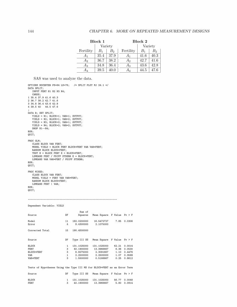
144 CHAPTER 6. MORE ON REPEATED MEASUREMENT DESIGNS
Block 1Variety
Fertility B1 B2
A1 35.4 37.9A2 36.7 38.2A3 34.8 36.4A4 39.5 40.0
Block 2Variety
Fertility B1 B2
A1 41.6 40.3A2 42.7 41.6A3 43.6 42.8A4 44.5 47.6
SAS was used to analyze the data.
OPTIONS NOCENTER PS=64 LS=76; /* SPLIT PLOT MJ 24.1 */DATA SPLIT;
INPUT FERT N1 N2 N3 N4;CARDS;
1 35.4 37.9 41.6 40.32 36.7 38.2 42.7 41.63 34.8 36.4 43.6 42.84 39.5 40 44.5 47.6;DATA B; SET SPLIT;
YIELD = N1; BLOCK=1; VAR=1; OUTPUT;YIELD = N2; BLOCK=1; VAR=2; OUTPUT;YIELD = N3; BLOCK=2; VAR=1; OUTPUT;YIELD = N4; BLOCK=2; VAR=2; OUTPUT;DROP N1--N4;
RUN;QUIT;
PROC GLM;CLASS BLOCK VAR FERT;MODEL YIELD = BLOCK FERT BLOCK*FERT VAR VAR*FERT;RANDOM BLOCK BLOCK*FERT;TEST H = BLOCK FERT E = BLOCK*FERT;LSMEANS FERT / PDIFF STDERR E = BLOCK*FERT;LSMEANS VAR VAR*FERT / PDIFF STDERR;
RUN;QUIT;
PROC MIXED;CLASS BLOCK VAR FERT;MODEL YIELD = FERT VAR VAR*FERT;RANDOM BLOCK BLOCK*FERT;LSMEANS FERT | VAR;
RUN;QUIT;
--------------------------------------------------------------
Dependent Variable: YIELD
Sum ofSource DF Squares Mean Square F Value Pr > F
Model 11 182.0200000 16.5472727 7.85 0.0306Error 4 8.4300000 2.1075000
Corrected Total 15 190.4500000
Source DF Type III SS Mean Square F Value Pr > F
BLOCK 1 131.1025000 131.1025000 62.21 0.0014FERT 3 40.1900000 13.3966667 6.36 0.0530BLOCK*FERT 3 6.9275000 2.3091667 1.10 0.4476VAR 1 2.2500000 2.2500000 1.07 0.3599VAR*FERT 3 1.5500000 0.5166667 0.25 0.8612
Tests of Hypotheses Using the Type III MS for BLOCK*FERT as an Error Term
Source DF Type III SS Mean Square F Value Pr > F
BLOCK 1 131.1025000 131.1025000 56.77 0.0048FERT 3 40.1900000 13.3966667 5.80 0.0914

6.2. THE SPLIT-PLOT DESIGN 145
We may reorganize the ANOVA table in the output as
Source DF SS Mean Square F Value Pr > F
BLOCK 1 131.1025000 131.1025000FERT 3 40.1900000 13.3966667 5.80 0.0914BLOCK*FERT=Error(Whole plot) 3 6.9275000 2.3091667VAR 1 2.2500000 2.2500000 1.07 0.3599VAR*FERT 3 1.5500000 0.5166667 0.25 0.8612Error(Subplot) 4 8.4300000 2.1075000
There is no significant difference among fertilizers. If this test were significant, them multiple comparisonswould have to be carried out to determine the significant differences. A slight modification of the SAS codeabove will provide the necessary tests. This is left as an exercise.

146 CHAPTER 6. MORE ON REPEATED MEASUREMENT DESIGNS
6.3 Crossover Designs
A crossover design is a two-way RM design in which the order (A) of administration of the repeated levelsof a single factor (B) is accounted for as a between subject factor in the design. Hence, a crossover design isa basic one-way RM design on the levels of B that has been analyzed as a two way RM design to account forthe order or sequence effect caused by the fact that the B levels are given one at a time in different orders.
A Latin square type design approach is used in the construction of the order effects so that each level jof B occurs equally often as the ith observation for i = 1, · · · , b.
We will only consider the two-period crossover design as an illustration. Here the repeated factor B hastwo levels b1 and b2 which are observed in the order b1, b2 by subjects in sequence level 1 (a1) and in theorder b2, b1 by subjects in sequence level 2 (a2) as shown below:
Period: CSequence: A c1 c2
a1 b1 b2
a2 b2 b1
There are three factors: sequence A (a1 and a2), period C (c1 and c2), and treatment B (b1 and b2) in theexperiment. Let βj be the jth treatment effect, j = 1, 2, and γk be the kth period effect, k = 1, 2. Further, letτ1 be the effect on the second observation if b1 is observed first and τ2 be the effect on the second observationif b2 is observed first. Thus τ1 and τ2 are the carry-over effects observed in the second observation wheneverb1 and b2 are observed first, respectively. Let Yijk be the random variable which represents the observationcorresponding to sequence i, treatment j and period k. The following table gives the observations:
Period: CSequence: A c1 c2 Meana1 = (b1, b2) Y111 Y122 Y1..
a2 = (b2, b1) Y221 Y212 Y2..
Mean Y..1 Y..2
The model incorporates carry-over effects in the second observations but not in the observations madefirst.
E(Y111) = µ + β1 + γ1 E(Y221) = µ + β2 + γ1
E(Y122) = µ + τ1 + β2 + γ2 E(Y212) = µ + τ2 + β1 + γ2
One can show that
E(Y1.. − Y2..) =τ1 − τ2
2
E(Y.1. − Y.2.) = (β1 − β2)− τ1 − τ2
2E(Y111 − Y221) = β1 − β2
E(Y..1 − Y..2) = E
(Y111 − Y122
2− Y212 − Y221
2
)= (τ1 − τ2)− τ1 + τ2
2
The last expression shows that the AB and C effects are identical, i.e. AB and C are confounded.If there is no sequence effect (H0 : τ1 = τ2), then
A : E(Y1.. − Y2..) =τ1 − τ2
2= 0
B : E(Y.1. − Y.2.) = (β1 − β2)
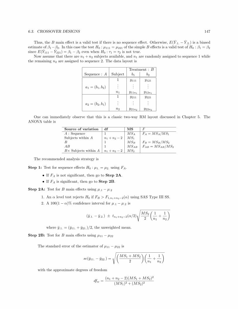
6.3. CROSSOVER DESIGNS 147
Thus, the B main effect is a valid test if there is no sequence effect. Otherwise, E(Y.1. − Y.2.) is a biasedestimate of β1−β2. In this case the test H0 : µ111 = µ221 of the simple B effects is a valid test of H0 : β1 = β2
since E(Y111 − Y221) = β1 − β2 even when H0 : τ1 = τ2 is not true.Now assume that there are n1 + n2 subjects available, and n1 are randomly assigned to sequence 1 while
the remaining n2 are assigned to sequence 2. The data layout is
Treatment : BSequence : A Subject b1 b2
1 y111 y121
a1 = (b1, b2)...
......
n1 y11n1 y12n1
1 y211 y221
a2 = (b2, b1)...
......
n2 y21n2 y22n2
One can immediately observe that this is a classic two-way RM layout discussed in Chapter 5. TheANOVA table is
Source of variation df MS F
A : Sequence 1 MSA FA = MSA/MS1
Subjects within A n1 + n2 − 2 MS1
B 1 MSB FB = MSB/MS2
AB 1 MSAB FAB = MSAB/MS2
B× Subjects within A n1 + n2 − 2 MS2
The recommended analysis strategy is
Step 1: Test for sequence effects H0 : µ1. = µ2. using FA.
• If FA is not significant, then go to Step 2A.
• If FA is significant, then go to Step 2B.
Step 2A: Test for B main effects using µ.1 − µ.2
1. An α level test rejects H0 if FB > F1,n1+n2−2(α) using SAS Type III SS.
2. A 100(1− α)% confidence interval for µ.1 − µ.2 is
(y.1. − y.2.) ± tn1+n2−2(α/2)
√MS2
2
(1n1
+1n2
)
where y.1. = (y11. + y21.)/2, the unweighted mean.
Step 2B: Test for B main effects using µ11 − µ22
The standard error of the estimator of µ11 − µ22 is
se(y11. − y22.) =
√(MS1 + MS2
2
)(1n1
+1n2
)
with the approximate degrees of freedom
dfw =(n1 + n2 − 2)(MS1 + MS2)2
(MS1)2 + (MS2)2
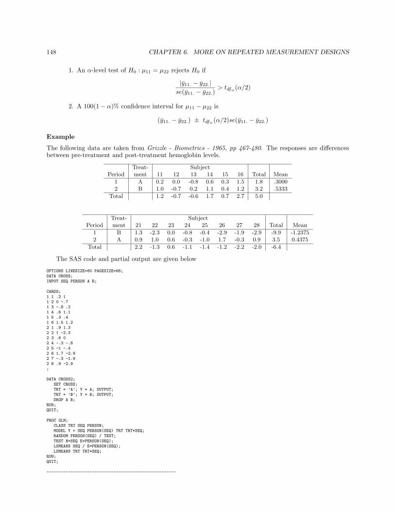
148 CHAPTER 6. MORE ON REPEATED MEASUREMENT DESIGNS
1. An α-level test of H0 : µ11 = µ22 rejects H0 if
|y11. − y22.|se(y11. − y22.)
> tdfw(α/2)
2. A 100(1− α)% confidence interval for µ11 − µ22 is
(y11. − y22.) ± tdfw(α/2)se(y11. − y22.)
Example
The following data are taken from Grizzle - Biometrics - 1965, pp 467-480. The responses are differencesbetween pre-treatment and post-treatment hemoglobin levels.
Treat- SubjectPeriod ment 11 12 13 14 15 16 Total Mean
1 A 0.2 0.0 -0.8 0.6 0.3 1.5 1.8 .30002 B 1.0 -0.7 0.2 1.1 0.4 1.2 3.2 .5333
Total 1.2 -0.7 -0.6 1.7 0.7 2.7 5.0
Treat- SubjectPeriod ment 21 22 23 24 25 26 27 28 Total Mean
1 B 1.3 -2.3 0.0 -0.8 -0.4 -2.9 -1.9 -2.9 -9.9 -1.23752 A 0.9 1.0 0.6 -0.3 -1.0 1.7 -0.3 0.9 3.5 0.4375
Total 2.2 -1.3 0.6 -1.1 -1.4 -1.2 -2.2 -2.0 -6.4
The SAS code and partial output are given below
OPTIONS LINESIZE=80 PAGESIZE=66;DATA CROSS;INPUT SEQ PERSON A B;
CARDS;1 1 .2 11 2 0 -.71 3 -.8 .21 4 .6 1.11 5 .3 .41 6 1.5 1.22 1 .9 1.32 2 1 -2.32 3 .6 02 4 -.3 -.82 5 -1 -.42 6 1.7 -2.92 7 -.3 -1.92 8 .9 -2.9;
DATA CROSS2;SET CROSS;TRT = ’A’; Y = A; OUTPUT;TRT = ’B’; Y = B; OUTPUT;DROP A B;
RUN;QUIT;
PROC GLM;CLASS TRT SEQ PERSON;MODEL Y = SEQ PERSON(SEQ) TRT TRT*SEQ;RANDOM PERSON(SEQ) / TEST;TEST H=SEQ E=PERSON(SEQ);LSMEANS SEQ / E=PERSON(SEQ);LSMEANS TRT TRT*SEQ;
RUN;QUIT;
------------------------------------------------------

6.3. CROSSOVER DESIGNS 149
Dependent Variable: Y
Sum ofSource DF Squares Mean Square F Value Pr > F
Model 15 27.96583333 1.86438889 1.50 0.2435Error 12 14.94416667 1.24534722
Corrected Total 27 42.91000000
Source DF Type III SS Mean Square F Value Pr > F
SEQ 1 4.57333333 4.57333333 3.67 0.0794PERSON(SEQ) 12 12.00666667 1.00055556 0.80 0.6446TRT 1 3.56297619 3.56297619 2.86 0.1165TRT*SEQ 1 6.24297619 6.24297619 5.01 0.0449
Tests of Hypotheses for Mixed Model Analysis of Variance
Dependent Variable: Y
Source DF Type III SS Mean Square F Value Pr > F* SEQ 1 4.573333 4.573333 4.57 0.0538
Error 12 12.006667 1.000556Error: MS(PERSON(SEQ))* This test assumes one or more other fixed effects are zero.
Least Squares Means
SEQ Y LSMEAN
1 0.416666672 -0.40000000
Least Squares Means
TRT Y LSMEAN
A 0.36875000B -0.35208333
TRT SEQ Y LSMEAN
A 1 0.30000000A 2 0.43750000B 1 0.53333333B 2 -1.23750000
Using SAS Type III analysis we get the following summary for α = .05 and α = .10 (for illustrativepurposes):
α = .05 : Sequence effects are not significant (p-value = .0538). Analyze treatment effects using y.1. = .3688and y.2. = −.3521. The difference is not significant (p-value = .1165). Therefore, there are no treatmenteffects at α = .05 level of significance.
α = .10 : Sequence effects are significant (p-value = .0538). Analyze treatment effects at time period 1 usingy11. = .3000 and y22. = −1.2375. We have
se(y11. − y22.) =
√(16
+18
)1.000 + 1.245
2= 0.572 ,
and
dfw =12(1 + 1.245)2
(1)2 + (1.245)2= 23.7 ≈ 24 .
Therefore, the t-statistic is.3000− (−1.2375)
.572= 2.69

150 CHAPTER 6. MORE ON REPEATED MEASUREMENT DESIGNS
which has a two-sided p-value of 0.0128.
Thus, the difference is significant at α = .10. Therefore, there are treatment effects at α = .10 level ofsignificance.

6.4. TWO-WAY REPEATED MEASUREMENT DESIGNS WITH REPEATED MEASURES ON BOTH FACTORS151
6.4 Two-Way Repeated Measurement Designs with Repeated Mea-sures on Both Factors
Consider a design where factors B and C are within subject factors with levels b and c, respectively. Assumethat a random sample of n subjects are observed on each of the bc crossed levels of B and C. The followingtable gives the data layout of such designs.
Treatments (B)B1 Bb
Subjects C1 · · · Cc · · · C1 · · · Cc
1 y111 y1c1 yb11 ybc1
......
......
...
n y11n y1cn yb1n ybcn
The statistical model for such designs is
yjkl = µ + βj + γk + (βγ)jk + Sl + (βS)jl + (γS)kl + (βγS)jkl + ejkl
for j = 1, . . . , b, k = 1, . . . , c, and l = 1, . . . , n, where
Fixed Effects :
• βj and γk ate the Bj and Ck main effects and
• (βγ)jk is the BjCk interaction effect.
Random Effects :
• Sl ∼ N(0, σ21) = subject l effect
• (βS)jl ∼ N(0, d2σ22) = Bj by subject l interaction.
• (γS)kl ∼ N(0, d3σ23) = Ck by subject l interaction.
• (βγS)jkl ∼ N(0, d4σ24) = Bj by Ck by subject l interaction.
• ejkl ∼ N(0, σ2).
We assume that the random effects interactions satisfy some (CS) conditions while all other randomvariables are assumed to be independent. One should notice that the ejkl are confounded with (βγS)jkl andhence cannot be estimated.
The following table contains the expected MS for the two-way RM design with repeated measures onboth factors. These are used in the construction of F tests.
Source df MS E(MS)Between Subjects
Subjects (S) n− 1 MSS σ2 + bcσ21
Within SubjectsB b− 1 MSb σ2 + cσ2
2 + ncb−1
∑β2
j
B × S (b− 1)(n− 1) MS1 σ2 + cσ22
C c− 1 MSc σ2 + bσ23 + nb
c−1
∑γ2
k
C × S (c− 1)(n− 1) MS2 σ2 + bσ23
BC (b− 1)(c− 1) MSbc σ2 + σ24 + n
(b−1)(c−1)
∑∑(βγ)jk
BC × S (b− 1)(c− 1)(n− 1) MS3 σ2 + σ24
The following ANOVA table gives the F tests to test for main effects:

152 CHAPTER 6. MORE ON REPEATED MEASUREMENT DESIGNS
Source df MS FBetween Subjects
Subjects (S) n− 1 MSS
Within SubjectsB b− 1 MSb Fb = MSb/MS1
B × S (b− 1)(n− 1) = df1 MS1
C c− 1 MSc Fc = MSc/MS2
C × S (c− 1)(n− 1) = df2
BC (b− 1)(c− 1) MSbc Fbc = MSbc/MS3
BC × S (b− 1)(c− 1)(n− 1) = df3 MS3
Mean comparisons are made using the following standard errors:
Parameter Estimate Standard Error dfMain Effects
βj − βj′ yj.. − yj′..
√2MS1
cn df1
γk − γk′ y.k. − y.k′.
√2MS2
bn df2
Simple Main Effects
µjk − µj′k yjk. − yj′k.
√2n
(df1MS1+df3MS3)(df1+df3
df4
µjk − µjk′ yjk. − yjk′.
√2n
(df2MS2+df3MS3)(df2+df3
df5
The degrees of freedoms for the simple main effects are approximated using Satterthwaite approximationformulae:
df4 =(df1MS1 + df3MS3)2
df1(MS1)2 + df3(MS3)2
df5 =(df2MS2 + df3MS3)2
df2(MS2)2 + df3(MS3)2
Three sphericity conditions corresponding to Fb, Fc, and Fbc need to be checked. If the (S) conditionis not satisfied, then G-G e-adjusted F tests followed by paired t tests for mean comparisons need to beperformed.
The generic SAS Proc GLM code for analyzing two-way repeated measurement designs with repeatedmeasures on both subjects is
PROC GLM;MODEL Y11 Y12 ... Ybc = / NOUNI;REPEATED B b, C c;
The following is part of an example taken from Milliken and Johnson, The Analysis of Messy Data, Vol. I.The attitiudes of families were measured every six months for three time periods. The data were obtained
for seven families, each family consisting of a son, father, and mother. The data are given as follows:
PersonSon Father Mother
Family T1 T2 T3 T1 T2 T3 T1 T2 T3
1 12 11 14 18 19 22 16 16 192 13 13 17 18 19 22 16 16 193 12 13 16 19 18 22 17 16 204 18 18 21 23 23 26 23 22 265 15 14 16 15 15 19 17 17 206 6 6 10 15 16 19 18 19 217 16 17 18 17 17 21 18 20 23

6.4. TWO-WAY REPEATED MEASUREMENT DESIGNS WITH REPEATED MEASURES ON BOTH FACTORS153
The SAS analysis of the data is given as follows:
DATA RM;
INPUT Y1-Y9;
CARDS;
12 11 14 18 19 22 16 16 19
13 13 17 18 19 22 16 16 19
12 13 16 19 18 22 17 16 20
18 18 21 23 23 26 23 22 26
15 14 16 15 15 19 17 17 20
6 6 10 15 16 19 18 19 21
16 17 18 17 17 21 18 20 23
;
PROC GLM;
MODEL Y1--Y9 = / NOUNI;
REPEATED B 3, C 3/ PRINTE NOM;
RUN;
QUIT;
DATA RM2;
SET RM;
ARRAY Z Y1--Y9;
DO I=1 TO 9;
Y = Z[I];
S = _N_;
IF (MOD(I,3) = 0) THEN DO;
B = ROUND(I/3);
C = ROUND(I/B);
OUTPUT;
END;
ELSE DO;
B = FLOOR(I/3) + 1;
C = MOD(I,3);
OUTPUT;
END;
END;
DROP Y1-Y9;
RUN;
QUIT;
PROC GLM DATA = RM2;
CLASS S B C;
MODEL Y = B|C|S;
TEST H=B E=B*S;
TEST H=C E=C*S;
TEST H=B*C E=B*C*S;
LSMEANS B/ PDIFF E=B*S;
LSMEANS C/PDIFF E=C*S;
LSMEANS B*C/PDIFF E=B*C*S;
RUN;
QUIT;
Some selected output from a run of the above program is:
Sphericity Tests(B)

154 CHAPTER 6. MORE ON REPEATED MEASUREMENT DESIGNS
Mauchly’s
Variables DF Criterion Chi-Square Pr > ChiSq
Transformed Variates 2 0.6961315 1.8110836 0.4043
Orthogonal Components 2 0.8660974 0.7187896 0.6981
Sphericity Tests(C)
Mauchly’s
Variables DF Criterion Chi-Square Pr > ChiSq
Transformed Variates 2 0.947328 0.2705497 0.8735
Orthogonal Components 2 0.6578854 2.0936229 0.3511
Sphericity Tests(BC)
Mauchly’s
Variables DF Criterion Chi-Square Pr > ChiSq
Transformed Variates 9 0.0508148 13.159756 0.1555
Orthogonal Components 9 0.0948413 10.403681 0.3188
The GLM Procedure
Repeated Measures Analysis of Variance
Univariate Tests of Hypotheses for Within Subject Effects
Adj Pr > F
Source DF Type III SS Mean Square F Value Pr > F G - G H - F
B 2 350.3809524 175.1904762 14.35 0.0007 0.0012 0.0007
Error(B) 12 146.5079365 12.2089947
Greenhouse-Geisser Epsilon 0.8819
Huynh-Feldt Epsilon 1.2212
Adj Pr > F
Source DF Type III SS Mean Square F Value Pr > F G - G H - F
C 2 144.8571429 72.4285714 258.28 <.0001 <.0001 <.0001
Error(C) 12 3.3650794 0.2804233
Greenhouse-Geisser Epsilon 0.7451
Huynh-Feldt Epsilon 0.9348
Adj Pr > F
Source DF Type III SS Mean Square F Value Pr > F G - G H - F
B*C 4 1.33333333 0.33333333 0.82 0.5262 0.4780 0.5237
Error(B*C) 24 9.77777778 0.40740741

6.4. TWO-WAY REPEATED MEASUREMENT DESIGNS WITH REPEATED MEASURES ON BOTH FACTORS155
LSMEAN
B Y LSMEAN Number
1 14.0952381 1
2 19.1904762 2
3 19.0000000 3
Least Squares Means for effect B
Pr > |t| for H0: LSMean(i)=LSMean(j)
Dependent Variable: Y
i/j 1 2 3
1 0.0005 0.0007
2 0.0005 0.8627
3 0.0007 0.8627
LSMEAN
C Y LSMEAN Number
1 16.2857143 1
2 16.4285714 2
3 19.5714286 3
Least Squares Means for effect C
Pr > |t| for H0: LSMean(i)=LSMean(j)
Dependent Variable: Y
i/j 1 2 3
1 0.3992 <.0001
2 0.3992 <.0001
3 <.0001 <.0001
LSMEAN
B C Y LSMEAN Number
1 1 13.1428571 1
1 2 13.1428571 2
1 3 16.0000000 3
2 1 17.8571429 4
2 2 18.1428571 5
2 3 21.5714286 6
3 1 17.8571429 7
3 2 18.0000000 8
3 3 21.1428571 9

156 CHAPTER 6. MORE ON REPEATED MEASUREMENT DESIGNS
Least Squares Means for effect B*C
Pr > |t| for H0: LSMean(i)=LSMean(j)
Dependent Variable: Y
i/j 1 2 3 4 5 6 7 8 9
1 1.0000 <.0001 <.0001 <.0001 <.0001 <.0001 <.0001 <.0001
2 1.0000 <.0001 <.0001 <.0001 <.0001 <.0001 <.0001 <.0001
3 <.0001 <.0001 <.0001 <.0001 <.0001 <.0001 <.0001 <.0001
4 <.0001 <.0001 <.0001 0.4106 <.0001 1.0000 0.6791 <.0001
5 <.0001 <.0001 <.0001 0.4106 <.0001 0.4106 0.6791 <.0001
6 <.0001 <.0001 <.0001 <.0001 <.0001 <.0001 <.0001 0.2212
7 <.0001 <.0001 <.0001 1.0000 0.4106 <.0001 0.6791 <.0001
8 <.0001 <.0001 <.0001 0.6791 0.6791 <.0001 0.6791 <.0001
9 <.0001 <.0001 <.0001 <.0001 <.0001 0.2212 <.0001 <.0001
The following is a summary of the results:
1. The (S) condition is satisfied for all three tests B, C, and BC.
2. The BC(Person by Time) interaction is not significant (P = 0.5262).
3. The BC interaction is not significant (P = 0.5262).
4. The B(Person) main effect is significant (P = .0007)
5. Comparison of B(Person) means
B1 B3 B214.1 19.0 19.2
--------------
6. The C(Time) main effect is significant (P < .0001)
7. Comparison of C(Time) means
C1 C2 C316.3 16.4 19.6--------------

Chapter 7
Introduction to the Analysis ofCovariance
Analysis of covariance (ANCOVA) methods combine regression and ANOVA techniques to investigate therelationship of a response variable with a set of ’treatments’ as well as other additional ’background’ variables.
7.1 Simple Linear Regression
Let y be a measured response variable that is believed to depend on a predictor x up to a random error;that is,
y = f(x) + ε; .
In a data setting, suppose we have n experimental units giving rise to observations (x1, y1), (x2, y2), · · · , (xn, yn).Then our model becomes
yi = f(xi) + εi, i = 1, 2, · · · , n .
In this chapter we will focus our attention to situations where y depends on x in a linear fashion; that is,
f(x) = β0 + β1x ,
where β0 is the intercept and β1 is the slope. In a data setting,
yi = β0 + β1xi + εi, i = 1, 2, · · · , n ,
where β0 and β1 are unknown. We will assume that the random errors, εi, are independent random variableswith mean 0 and constant variance σ2.
Our goal is to estimate and make inferences about the unknown regression coefficients, β0 and β1.
7.1.1 Estimation : The Method of Least Squares
The least squares (LS) estimators β0 and β1 of β0 and β1, respectively, are the values of β0 and β1 thatminimize
L(β0, β1) =n∑
i=1
ε2i =
n∑
i=1
(yi − β0 − β1xi)2 .
Thus the observation yi is estimated by the fitted value
yi = β0 + β1xi .
In other words, the method of least squares gives the least possible sum of squared residuals, yi − yi.Using differential calculus, we get the LS estimators as
157

158 CHAPTER 7. INTRODUCTION TO THE ANALYSIS OF COVARIANCE
β1 =Sxy
Sxx, and β0 = y − β1x ,
where
Sxy =n∑
i=1
(xi − x)(yi − y) and Sxx =n∑
i=1
(xi − x)2 .
7.1.2 Partitioning the Total SS
Similar to ANOVA models, the total sum of squares∑
(yi − y)2 partitions into smaller variabilities: thevariability in the response explained by the regression model and the unexplained variability. This is doneas
n∑
i=1
(yi − y)2 =n∑
i=1
(yi − y)2 +n∑
i=1
(yi − y)2
i.e.,SST = SSR + SSE .
Here SSR represents the sum of squares due to regression while SST and SSE are the familiar SS’s due tototal and error, respectively. As before the degrees of freedom for SST partitions into regression df and errordf as
n− 1 = 1 + (n− 2) .
7.1.3 Tests of Hypotheses
One very important question is ”Does x truly influence y?”. Since this is under an assumption of a linearrelationship, another way to pose the question will be ”Is there a significant linear relationship between xand y?” In terms of statistical hypotheses, we are interested in testing
H0 : β1 = 0HA : β1 6= 0
The rejection of H0 indicates that there is a significant linear relationship between x and y. It does not,however, imply that the model is ”good”.
Using the partition of the total variability, one may set up an ANOVA table as follows:
Source df SS MS FRegression 1 SSR MSR = SSR/1 F = MSR/MSE
Residual n− 2 SSE MSE = SSE/(n− 2)
Total n− 1 SST
We reject the null if the F -test is significant at the desired level of significance.
Example
Let X be the length (cm) of a laboratory mouse and let Y be its weight (gm). Consider the data for X andY given below.
X Y16 3215 2620 4013 2715 30

7.1. SIMPLE LINEAR REGRESSION 159
17 3816 3421 4322 6423 4524 4618 39
The following SAS code is used to perform the simple linear regression.
DATA SLR;
INPUT X Y;
CARDS;
16 32
15 26
20 40
13 27
15 30
17 38
16 34
21 43
22 64
23 45
24 46
18 39
;
SYMBOL V=CIRCLE I=NONE;
PROC GPLOT;
TITLE1 ’SCATTER PLOT OF Y VS X’;
PLOT Y*X;
RUN;
QUIT;
PROC GLM;
TITLE1 ’REGRESSION OF Y ON X’;
MODEL Y = X;
OUTPUT OUT=REGOUT R=R P=P;
RUN;
QUIT;
SYMBOL V=CIRCLE I=R;
PROC GPLOT DATA=SLR;
TITLE1 ’SCATTER PLOT OF Y VS X OVERLAYED WITH REGRESSION FIT’;
PLOT Y*X;
RUN;
QUIT;
PROC GPLOT DATA=REGOUT;
TITLE1 ’RESIDUAL PLOT’;
PLOT R*P;
RUN;
QUIT;
Selected output from SAS is given below:

160 CHAPTER 7. INTRODUCTION TO THE ANALYSIS OF COVARIANCE
Dependent Variable: Y
Sum of
Source DF Squares Mean Square F Value Pr > F
Model 1 813.763823 813.763823 21.36 0.0009
Error 10 380.902844 38.090284
Corrected Total 11 1194.666667
R-Square Coeff Var Root MSE Y Mean
0.681164 15.96138 6.171733 38.66667
Source DF Type I SS Mean Square F Value Pr > F
X 1 813.7638231 813.7638231 21.36 0.0009
Source DF Type III SS Mean Square F Value Pr > F
X 1 813.7638231 813.7638231 21.36 0.0009
Standard
Parameter Estimate Error t Value Pr > |t|
Intercept -5.428909953 9.70503506 -0.56 0.5882
X 2.405213270 0.52036911 4.62 0.0009

7.1. SIMPLE LINEAR REGRESSION 161
The fitted regression line isy = −5.43 + 2.41x
The length of a mouse is significantly linearly related to the weight of a mouse (P = 0.0009). From thescatter plot and the fitted line, one observes that the relationship between length and weight is an increasingrelationship.
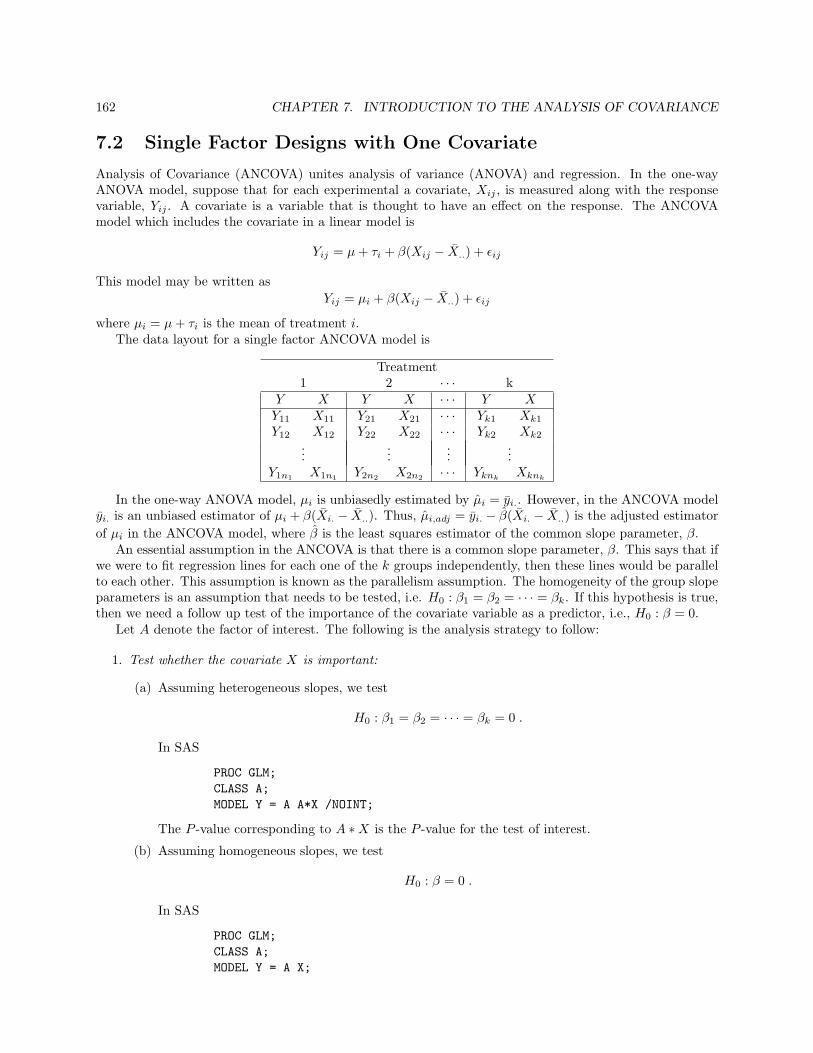
162 CHAPTER 7. INTRODUCTION TO THE ANALYSIS OF COVARIANCE
7.2 Single Factor Designs with One Covariate
Analysis of Covariance (ANCOVA) unites analysis of variance (ANOVA) and regression. In the one-wayANOVA model, suppose that for each experimental a covariate, Xij , is measured along with the responsevariable, Yij . A covariate is a variable that is thought to have an effect on the response. The ANCOVAmodel which includes the covariate in a linear model is
Yij = µ + τi + β(Xij − X..) + εij
This model may be written asYij = µi + β(Xij − X..) + εij
where µi = µ + τi is the mean of treatment i.The data layout for a single factor ANCOVA model is
Treatment1 2 · · · k
Y X Y X · · · Y XY11 X11 Y21 X21 · · · Yk1 Xk1
Y12 X12 Y22 X22 · · · Yk2 Xk2
......
......
Y1n1 X1n1 Y2n2 X2n2 · · · YknkXknk
In the one-way ANOVA model, µi is unbiasedly estimated by µi = yi.. However, in the ANCOVA modelyi. is an unbiased estimator of µi + β(Xi. − X..). Thus, µi,adj = yi. − β(Xi. − X..) is the adjusted estimatorof µi in the ANCOVA model, where β is the least squares estimator of the common slope parameter, β.
An essential assumption in the ANCOVA is that there is a common slope parameter, β. This says that ifwe were to fit regression lines for each one of the k groups independently, then these lines would be parallelto each other. This assumption is known as the parallelism assumption. The homogeneity of the group slopeparameters is an assumption that needs to be tested, i.e. H0 : β1 = β2 = · · · = βk. If this hypothesis is true,then we need a follow up test of the importance of the covariate variable as a predictor, i.e., H0 : β = 0.
Let A denote the factor of interest. The following is the analysis strategy to follow:
1. Test whether the covariate X is important:
(a) Assuming heterogeneous slopes, we test
H0 : β1 = β2 = · · · = βk = 0 .
In SAS
PROC GLM;CLASS A;MODEL Y = A A*X /NOINT;
The P -value corresponding to A ∗X is the P -value for the test of interest.
(b) Assuming homogeneous slopes, we test
H0 : β = 0 .
In SAS
PROC GLM;CLASS A;MODEL Y = A X;

7.2. SINGLE FACTOR DESIGNS WITH ONE COVARIATE 163
If both are non-significant, then the covariate X is not needed. If either one of the tests is significant,the we use the ANCOVA model. Go to Step 2.
2. Test whether there is a common slope:We test
H0 : β1 = β2 = · · · = βk
using
PROC GLM;CLASS A;MODEL Y = A X A*X;
The P -value of interest corresponds to the A ∗X term.
(a) If the test is significant, then we follow a Johnson-Neyman analysis. This will be addressed in alater section.
(b) If the test is not significant, then we perform the ANCOVA analysis. Using SAS
PROC GLM;CLASS A;MODEL Y = A X;
fits the classic ANCOVA model
Yij = µ + τi + β(Xij − X..) + εij
and tests H0 : τ1 = τ2 = · · · = τk = 0.Follow-up pairwise comparisons (H0 : τi = τj) may be performed by including
LSMEANS A/PDIFF;
in the preceding SAS code.
The following example is adapted from Snedecor and Cochran (1967) (See also SAS Online Documenta-tion).
Example
Ten patients are selected for each treatment (Drug), and six sites on each patient are measured for leprosybacilli. The variables in the study are
• Drug - two antibiotics (A and D) and a control (F)
• PreTreatment - a pre-treatment score of leprosy bacilli
• PostTreatment - a post-treatment score of leprosy bacilli
The covariate (a pretreatment score) is included in the model for increased precision in determining theeffect of drug treatments on the posttreatment count of bacilli.
The following is the SAS code used to analyze the data. It is given along with a partial output.
DATA DRUGTEST;input DRUG $ PRE POST @@;CARDS;
A 11 6 A 8 0 A 5 2 A 14 8 A 19 11A 6 4 A 10 13 A 6 1 A 11 8 A 3 0D 6 0 D 6 2 D 7 3 D 8 1 D 18 18

164 CHAPTER 7. INTRODUCTION TO THE ANALYSIS OF COVARIANCE
D 8 4 D 19 14 D 8 9 D 5 1 D 15 9F 16 13 F 13 10 F 11 18 F 9 5 F 21 23F 16 12 F 12 5 F 12 16 F 7 1 F 12 20
;
PROC GLM;CLASS DRUG;MODEL POST = DRUG DRUG*PRE / NOINT;
RUN;QUIT;
PROC GLM;CLASS DRUG;MODEL POST = DRUG PRE DRUG*PRE;
RUN;QUIT;
PROC GLM;CLASS DRUG;MODEL POST = DRUG PRE;MEANS DRUG;LSMEANS DRUG/ STDERR PDIFF TDIFF;
RUN;QUIT;
---------------------------------------------------------------------------
Dependent Variable: POSTSum of
Source DF Squares Mean Square F Value Pr > FDRUG 3 2165.900000 721.966667 43.58 <.0001PRE*DRUG 3 597.542048 199.180683 12.02 <.0001Error 24 397.557952 16.564915Total 30 3161.000000
Dependent Variable: POSTSum of
Source DF Squares Mean Square F Value Pr > FDRUG 2 293.6000000 146.8000000 8.86 0.0013PRE 1 577.8974030 577.8974030 34.89 <.0001PRE*DRUG 2 19.6446451 9.8223226 0.59 0.5606Error 24 397.557952 16.564915Total 29 1288.700000
Dependent Variable: POSTSum of
Source DF Squares Mean Square F Value Pr > FDRUG 2 293.6000000 146.8000000 9.15 0.0010PRE 1 577.8974030 577.8974030 36.01 <.0001

7.2. SINGLE FACTOR DESIGNS WITH ONE COVARIATE 165
Error 26 417.202597 16.046254Total 29 1288.700000
Level of -------------POST------------ -------------PRE-------------DRUG N Mean Std Dev Mean Std Dev
A 10 5.3000000 4.64399254 9.3000000 4.76211904D 10 6.1000000 6.15449249 10.0000000 5.24933858F 10 12.3000000 7.14998057 12.9000000 3.95671019
Standard LSMEANDRUG POST LSMEAN Error Pr > |t| NumberA 6.7149635 1.2884943 <.0001 1D 6.8239348 1.2724690 <.0001 2F 10.1611017 1.3159234 <.0001 3
Least Squares Means for Effect DRUGt for H0: LSMean(i)=LSMean(j) / Pr > |t|
Dependent Variable: POST
i/j 1 2 3
1 -0.0607 -1.826460.9521 0.0793
2 0.060704 -1.800110.9521 0.0835
3 1.826465 1.8001120.0793 0.0835
An observation is that the results of MEANS and LSMEANS are quite different. LSMEANS gives theadjusted means while MEANS gives the raw means. Here is a summary of the results:
1. Is the covariate important?
(a) The hypothesis H0 : β1 = β2 = β3 = 0 is rejected (F = 12.02, P < 0.0001).
(b) The hypothesis H0 : β = 0 is rejected (F = 36.01, P < 0.0001).
Thus, the covariate is important and needs to be included in the model.
2. Do we have a common slope?We fail to reject the hypothesis H0 : β1 = β2 = β3 (F = 0.59, P = 0.5606). Thus, the assumption of acommon slope is a valid assumption.
The test for treatment effects, H0 : τ1 = τ2 = τ3 = 0, is significant (F = 9.15, P = 0.0010).
None of the pairwise differences is significant at α = .05.

166 CHAPTER 7. INTRODUCTION TO THE ANALYSIS OF COVARIANCE
7.3 ANCOVA in Randomized Complete Block Designs
We will consider the case where a single covariate is observed along with the response in a RCBD. Theanalysis of such a design proceeds in the same manner as the single factor design considered above.
The statistical model for the RCBD ANCOVA is
Yij = µ + τi + γj + β(Xij − X..) + εij
where i = 1, · · · , k, j = 1, · · · , n, and γj is the effect of the jth block of n blocks.Let A denote the factor of interest and B be the blocking factor. The following is the analysis strategy
to follow:
1. Test whether the covariate X is important:
(a) Assuming heterogeneous slopes, we test
H0 : β1 = β2 = · · · = βk = 0 .
In SAS
PROC GLM;CLASS A;MODEL Y = A B A*X /NOINT;
The P -value corresponding to A ∗X is the P -value for the test of interest.
(b) Assuming homogeneous slopes, we test
H0 : β = 0 .
In SAS
PROC GLM;CLASS A;MODEL Y = A B X;
If both are non-significant, then the covariate X is not needed. If either one of the tests is significant,the we use the ANCOVA model. Go to Step 2.
2. Test whether there is a common slope:We test
H0 : β1 = β2 = · · · = βk
using
PROC GLM;CLASS A;MODEL Y = A B X A*X;
The P -value of interest corresponds to the A ∗X term.
(a) If the test is significant, then we follow a Johnson-Neyman type analysis.
(b) If the test is not significant, then we perform the ANCOVA analysis. Using SAS
PROC GLM;CLASS A;MODEL Y = A B X;

7.3. ANCOVA IN RANDOMIZED COMPLETE BLOCK DESIGNS 167
fits the RCBD ANCOVA model
Yij = µ + τi + γj + β(Xij − X..) + εij
and tests H0 : τ1 = τ2 = · · · = τk = 0.Follow-up pairwise comparisons (H0 : τi = τj) may be performed by including
LSMEANS A/PDIFF;
in the preceding SAS code.
The following example is taken from Wishart (1949).
Example
Yields for 3 varieties of a certain crop in a randomized complete block design with 4 blocks are considered.The variables of interest are
• X = yield of a plot in a previous year
• Y = yield on the same plot for the experimental year
The data are as follows:
VarietiesBlock A B C1 X 54 51 57
Y 64 65 72
2 X 62 64 60Y 68 69 70
3 X 51 47 46Y 54 60 57
4 X 53 50 41Y 62 66 61
The SAS analysis of the data is as follows:
DATA CROP;INPUT A $ B Y X;CARDS;
A 1 64 54A 2 68 62A 3 54 51A 4 62 53B 1 65 51B 2 69 64B 3 60 47B 4 66 50C 1 72 57C 2 70 60C 3 57 46C 4 61 41
;
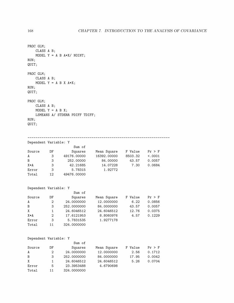
168 CHAPTER 7. INTRODUCTION TO THE ANALYSIS OF COVARIANCE
PROC GLM;CLASS A B;MODEL Y = A B A*X/ NOINT;
RUN;QUIT;
PROC GLM;CLASS A B;MODEL Y = A B X A*X;
RUN;QUIT;
PROC GLM;CLASS A B;MODEL Y = A B X;LSMEANS A/ STDERR PDIFF TDIFF;
RUN;QUIT;
-----------------------------------------------------------------------Dependent Variable: Y
Sum ofSource DF Squares Mean Square F Value Pr > FA 3 49176.00000 16392.00000 8503.32 <.0001B 3 252.00000 84.00000 43.57 0.0057X*A 3 42.21685 14.07228 7.30 0.0684Error 3 5.78315 1.92772Total 12 49476.00000
Dependent Variable: YSum of
Source DF Squares Mean Square F Value Pr > FA 2 24.0000000 12.0000000 6.22 0.0856B 3 252.0000000 84.0000000 43.57 0.0057X 1 24.6046512 24.6046512 12.76 0.0375X*A 2 17.6121953 8.8060976 4.57 0.1229Error 3 5.7831535 1.9277178Total 11 324.0000000
Dependent Variable: YSum of
Source DF Squares Mean Square F Value Pr > FA 2 24.0000000 12.0000000 2.56 0.1712B 3 252.0000000 84.0000000 17.95 0.0042X 1 24.6046512 24.6046512 5.26 0.0704Error 5 23.3953488 4.6790698Total 11 324.0000000

7.3. ANCOVA IN RANDOMIZED COMPLETE BLOCK DESIGNS 169
Least Squares Means
Standard LSMEANA Y LSMEAN Error Pr > |t| Number
A 60.9302326 1.1778789 <.0001 1B 65.0000000 1.0815579 <.0001 2C 66.0697674 1.1778789 <.0001 3
Least Squares Means for Effect At for H0: LSMean(i)=LSMean(j) / Pr > |t|
Dependent Variable: Y
i/j 1 2 3
1 -2.54501 -2.868580.0516 0.0351
2 2.545014 -0.668980.0516 0.5332
3 2.868582 0.6689750.0351 0.5332
The covariate X does not appear to be very important (P = 0.0684 for heterogeneous slopes and P =0.0704 for a single slope). However, we will keep it in the analysis for the sake of illustration. Besides, withP -values close to 0.05, this is the conservative route to follow.
The test for the equality of slopes is not rejected (P = 0.1229). Thus, the assumption of a common slopeis justified.
The test for treatment effect is not significant. Hence, we fail to detect any difference in yield among the3 different crop varieties after adjusting for yield differences of the previous year.
The results of the pairwise testing are summarized below using underlining.
Group A B C60.9302326 65.0000000 66.0697674
--------------------------

170 CHAPTER 7. INTRODUCTION TO THE ANALYSIS OF COVARIANCE
7.4 ANCOVA in Two-Factor Designs
We will start by recalling the balanced two-factor fixed effects analysis of variance model
yijk = µ + τi + γj + (τγ)ij + εijk,
i = 1, . . . , a
j = 1, . . . , b
k = 1, . . . , n
wherea∑
i=1
τi =b∑
j=1
γj =a∑
i=1
(τγ)ij =b∑
j=1
(τγ)ij = 0 .
and εijk ∼iid N(0, σ2).We shall consider the case where a covariate xijk is observed along with the response for each experimental
unit. The corresponding two-factor fixed effects ANCOVA model is
yijk = µ + τi + γj + (τγ)ij + β(xijk − x...) + εijk,
i = 1, . . . , a
j = 1, . . . , b
k = 1, . . . , n
under the same assumptions.As in the one-way model, the means µi., µ.j , and µij are estimated by the adjusted means
µi. = yi.. − β(xi.. − x...)
µ.j = y.j. − β(x.j. − x...)
µij = yij. − β(xij. − x...)
The major assumption, once again, is the homogeneity of the slopes. If that assumption is not satisfied,then our model may be written as
yijk = µ + τi + γj + (τγ)ij + βij(xijk − x...) + εijk,
i = 1, . . . , a
j = 1, . . . , b
k = 1, . . . , n
under the same assumptions as above. Thus, the hypothesis
H0 : β11 = . . . = βab = β
is of interest. We may use the one-way ANCOVA methods to perform the test by rewriting the model as
ysk = µs + βs(xsk − x...) + εsk,
{s = 1, . . . , ab
k = 1, . . . , n
which is obtained by ”rolling-out” the cells into one big vector as
(i,j) (1,1) (1,2) · · · (a, b-1) (a,b)s 1 2 · · · ab - 1 ab
The correspondence between s and (i, j) is according to the formula
s = b(i− 1) + j .
The analysis of two-way ANCOVA is performed as follows:
1. Test for the homogeneity of the slopes.
2. If the slopes are not heterogeneous, test main and simple effects using the adjusted means. If the slopesare heterogeneous, use a Johnson-Neyman analysis.
The following example is taken from Neter, Kutner, Nachtsheim, and Wasserman. Applied Linear Sta-tistical Models.

7.4. ANCOVA IN TWO-FACTOR DESIGNS 171
Example
A horticulturist conducted an experiment to study the effects of flower variety (factor A) and moisture level(factor B) on yield of salable flowers (Y ). Because the plots were not of the same size, the horticulturistwished to use plot size (X) as the concomitant variable. Six replications were made for each treatment. Thedata are presented below:
Factor BB1 (low) B2 (high)
Factor A Yi1k Xi1k Yi2k Xi2k
A1 (variety LP) 98 15 71 1060 4 80 1277 7 86 1480 9 82 1395 14 46 264 5 55 3
A2 (variety WB) 55 4 76 1160 5 68 1075 8 43 265 7 47 387 13 62 778 11 70 9
The following SAS code is used to analyze the above example. A partial output is given following thecode:
DATA FLOWERS;INPUT A B Y X @@;C = 2*(A-1)+B;CARDS;
1 1 98 15 1 2 71 101 1 60 4 1 2 80 121 1 77 7 1 2 86 141 1 80 9 1 2 82 131 1 95 14 1 2 46 21 1 64 5 1 2 55 32 1 55 4 2 2 76 112 1 60 5 2 2 68 102 1 75 8 2 2 43 22 1 65 7 2 2 47 32 1 87 13 2 2 62 72 1 78 11 2 2 70 9
;
PROC GLM;TITLE1 ’HOMOGENEITY OF SLOPES’;CLASS C;MODEL Y = C X C*X;
RUN;QUIT;
PROC GLM;TITLE1 ’TWO-WAY ANCOVA’;

172 CHAPTER 7. INTRODUCTION TO THE ANALYSIS OF COVARIANCE
CLASS A B;MODEL Y = A B A*B X;LSMEANS A B A*B / STDERR PDIFF TDIFF;
RUN;QUIT;
-----------------------------------------------------------------------------HOMOGENEITY OF SLOPES
Dependent Variable: Y
Sum ofSource DF Squares Mean Square F Value Pr > FC 3 87.399785 29.133262 4.29 0.0212X 1 3703.309097 3703.309097 544.87 <.0001X*C 3 10.733375 3.577792 0.53 0.6704Error 16 108.747808 6.796738Total 23 5086.000000
TWO-WAY ANCOVADependent Variable: Y
Sum ofSource DF Squares Mean Square F Value Pr > FA 1 96.601826 96.601826 15.36 0.0009B 1 323.849473 323.849473 51.50 <.0001A*B 1 16.042244 16.042244 2.55 0.1267X 1 3994.518817 3994.518817 635.21 <.0001Error 19 119.481183 6.288483Total 23 5086.000000
Least Squares Means
Standard H0:LSMEAN=0 H0:LSMean1=LSMean2A Y LSMEAN Error Pr > |t| t Value Pr > |t|1 72.0423387 0.7304444 <.0001 3.92 0.00092 67.9576613 0.7304444 <.0001
Standard H0:LSMEAN=0 H0:LSMean1=LSMean2B Y LSMEAN Error Pr > |t| t Value Pr > |t|1 73.6807796 0.7246356 <.0001 7.18 <.00012 66.3192204 0.7246356 <.0001
Standard LSMEANA B Y LSMEAN Error Pr > |t| Number1 1 76.5423387 1.0283916 <.0001 11 2 67.5423387 1.0283916 <.0001 22 1 70.8192204 1.0242739 <.0001 32 2 65.0961022 1.0365780 <.0001 4
Least Squares Means for Effect A*B

7.4. ANCOVA IN TWO-FACTOR DESIGNS 173
t for H0: LSMean(i)=LSMean(j) / Pr > |t|
Dependent Variable: Y
i/j 1 2 3 4
1 6.216274 3.937098 7.781373<.0001 0.0009 <.0001
2 -6.21627 -2.25426 1.662999<.0001 0.0362 0.1127
3 -3.9371 2.254261 3.9370980.0009 0.0362 0.0009
4 -7.78137 -1.663 -3.9371<.0001 0.1127 0.0009
Thus
1. The parallelism hypothesisH0 : β11 = β12 = β21 = β22 = β
is not rejected (P = 0.6704). The ANCOVA model with a common slope is valid.
2. Comparisons of means results:
(a) The AB interaction effect fails to be significant (P = 0.1267). We may compare A and B meansat the main effect level.
(b) The A main effect is significant (P = 0.0009).
(c) The B main effect is significant (P < 0.0001).
(d) The hypothesis H0 : β = 0 is rejected (P < 0.0001). Thus the inclusion of the covariate is justified.
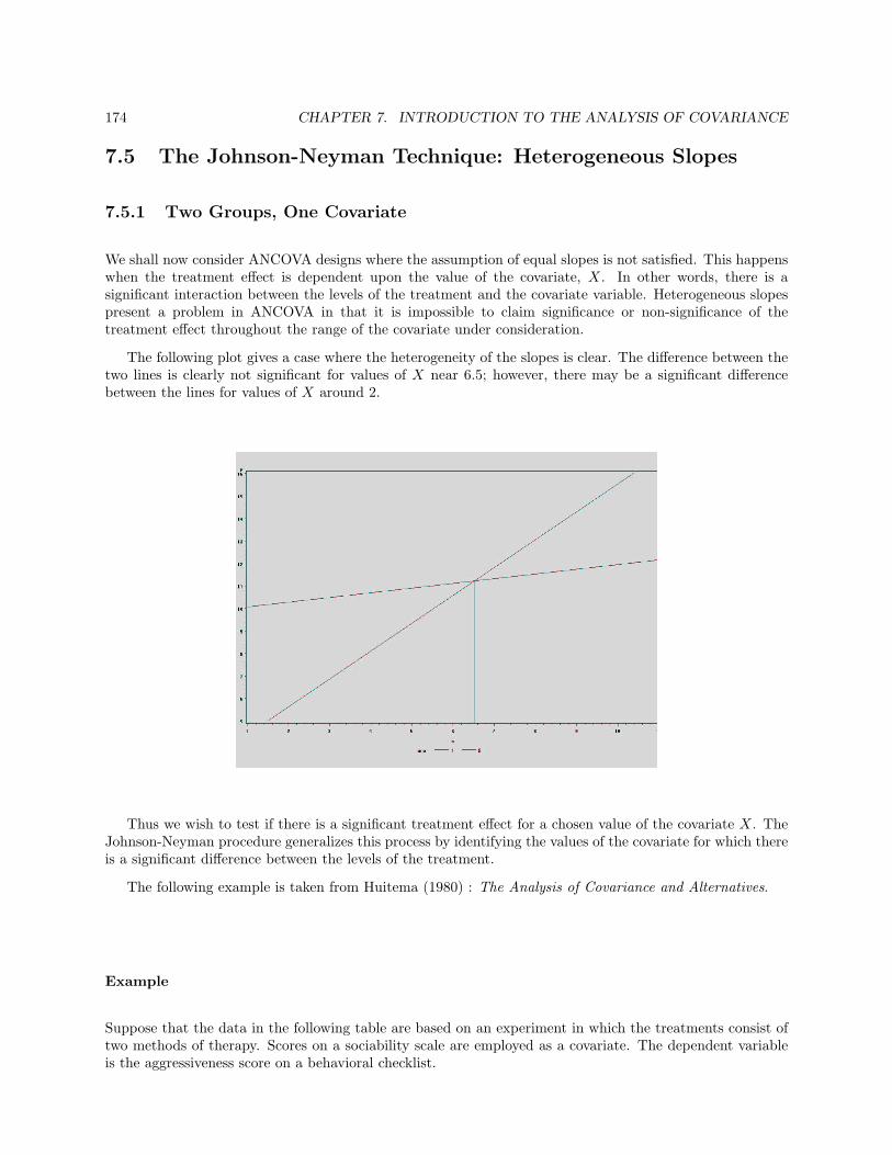
174 CHAPTER 7. INTRODUCTION TO THE ANALYSIS OF COVARIANCE
7.5 The Johnson-Neyman Technique: Heterogeneous Slopes
7.5.1 Two Groups, One Covariate
We shall now consider ANCOVA designs where the assumption of equal slopes is not satisfied. This happenswhen the treatment effect is dependent upon the value of the covariate, X. In other words, there is asignificant interaction between the levels of the treatment and the covariate variable. Heterogeneous slopespresent a problem in ANCOVA in that it is impossible to claim significance or non-significance of thetreatment effect throughout the range of the covariate under consideration.
The following plot gives a case where the heterogeneity of the slopes is clear. The difference between thetwo lines is clearly not significant for values of X near 6.5; however, there may be a significant differencebetween the lines for values of X around 2.
Thus we wish to test if there is a significant treatment effect for a chosen value of the covariate X. TheJohnson-Neyman procedure generalizes this process by identifying the values of the covariate for which thereis a significant difference between the levels of the treatment.
The following example is taken from Huitema (1980) : The Analysis of Covariance and Alternatives.
Example
Suppose that the data in the following table are based on an experiment in which the treatments consist oftwo methods of therapy. Scores on a sociability scale are employed as a covariate. The dependent variableis the aggressiveness score on a behavioral checklist.

7.5. THE JOHNSON-NEYMAN TECHNIQUE: HETEROGENEOUS SLOPES 175
Therapy 1 Therapy 1X Y X Y1 10 1 52 10 1.5 62 11 2.5 63 10 3.5 74 11 4.5 85 11 4.5 95 10 5 96 11 6 96 11.5 6 10.57 12 7 118 12 7 12.58 11 7.5 12.59 11 8 1410 12.5 9 14.511 12 10 16
Using SAS, we get the following two regression lines:
The slopes are heterogeneous. The following SAS code may be used to fit the heterogeneous slopeANCOVA and test for significance of the difference between the two methods of therapy on a case by casebasis. A partial output is given following the code.
data jn;input grp x y;cards;
1 1 101 2 101 2 111 3 101 4 111 5 111 5 101 6 11

176 CHAPTER 7. INTRODUCTION TO THE ANALYSIS OF COVARIANCE
1 6 11.51 7 121 8 121 8 111 9 111 10 12.51 11 122 1 52 1.5 62 2.5 62 3.5 72 4.5 82 4.5 92 5 92 6 92 6 10.52 7 112 7 12.52 7.5 12.52 8 142 9 14.52 10 16
;
goptions reset=symbol;symbol1 c=black v=dot l=1 i=r;symbol2 c=black v=square l=1 i=r;
proc gplot;plot y*x=grp;
run;quit;
PROC GLM DATA=JN;CLASS GRP;MODEL Y = GRP X GRP*X;LSMEANS GRP/ AT X=5 PDIFF;LSMEANS GRP/ AT X=6.5 PDIFF TDIFF;LSMEANS GRP/ AT X=6.7 PDIFF TDIFF;LSMEANS GRP/ AT X=8 PDIFF TDIFF;
RUN;QUIT;
--------------------------------------------------------------------------Sum of
Source DF Squares Mean Square F Value Pr > Fgrp 1 64.1707155 64.1707155 152.79 <.0001x 1 117.7551731 117.7551731 280.37 <.0001x*grp 1 59.5963693 59.5963693 141.90 <.0001Error 26 10.9199841 0.4199994

7.5. THE JOHNSON-NEYMAN TECHNIQUE: HETEROGENEOUS SLOPES 177
Total 29 176.9666667
Least Squares Means at x=5H0:LSMean1=
LSMean2grp y LSMEAN Pr > |t|1 10.8997955 <.00012 9.3402754
Least Squares Means at x=6.5H0:LSMean1=LSMean2
grp y LSMEAN t Value Pr > |t|1 11.2126789 0.07 0.94612 11.1957508
Least Squares Means at x=6.7H0:LSMean1=LSMean2
grp y LSMEAN t Value Pr > |t|1 11.2543967 -0.74 0.46362 11.4431475
Least Squares Means at x=8H0:LSMean1=LSMean2
grp y LSMEAN t Value Pr > |t|1 11.5255624 -4.89 <.00012 13.0512261
Thus, there is a significant difference between the two methods of therapy for an individual with asociability scale of 5 (P < 0.0001), while we fail to find a significant treatment effect for an individual witha sociability scale of 6.5 (P = 0.9461).
Let the regression lines fitted individually for groups 1 and 2 be Y1 = α1 + β1X1 and Y2 = α2 + β2X2,respectively. Let X1 and X2 be the sample means of the covariate associated with the two groups while
SXX1 =n1∑
i=1
(X1i − X1)2, and SXX2 =n2∑
i=1
(X2i − X2)2
where n1 and n2 are the respective sample sizes.We can identify the lower and upper limits, XL and XU , of the region of non-significance on X using the
following formulæ:
XL =−B −√B2 −AC
A
XU =−B +
√B2 −AC
A
where
A = −d
(1
SXX1
+1
SXX2
)+ (β1 − β2)2
B = d
(X1
SXX1
+X2
SXX2
)+ (α1 − α2)(β1 − β2)
C = −d
(1n1
+1n2
+X2
1
SXX1
+X2
2
SXX2
)+ (α1 − α2)2

178 CHAPTER 7. INTRODUCTION TO THE ANALYSIS OF COVARIANCE
Hered = (tn1+n2−4(α/2))2s2
p
where
s2p =
(n1 − 2)s21 + (n2 − 2)s2
2
n1 + n2 − 4
is the pooled variance. The values of s21 and s2
2 represent the error mean of squares when the two individualregression lines are fit.
Example
Consider the preceding example. The following SAS code can be used to compute the quantities in theformula.
PROC SORT;BY GRP;
RUN;QUIT;
PROC MEANS MEAN CSS N;VAR X;BY GRP;
RUN;QUIT;
PROC GLM DATA=JN;MODEL Y = X;BY GRP;
RUN;QUIT;
/* Get t value squared from the T-table*/DATA T;
TVAL = TINV(.975, 26);TVAL = TVAL*TVAL;
RUN;QUIT;
PROC PRINT DATA=T;RUN;QUIT;
---------------------------------------------------------------------------------------------------------------------------- grp=1 ---------------------------
Analysis Variable : x
Mean Corrected SS N
5.8000000 130.4000000 15
--------------------------------------------- grp=2 ---------------------------Analysis Variable : x

7.5. THE JOHNSON-NEYMAN TECHNIQUE: HETEROGENEOUS SLOPES 179
Mean Corrected SS N
5.5333333 99.2333333 15
--------------------------------------------- grp=1 ---------------------------Sum of
Source DF Squares Mean Square F Value Pr > Fx 1 5.67361963 5.67361963 19.62 0.0007Error 13 3.75971370 0.28920875Total 14 9.43333333
StandardParameter Estimate Error t Value Pr > |t|Intercept 9.856850716 0.30641368 32.17 <.0001x 0.208588957 0.04709414 4.43 0.0007
--------------------------------------------- grp=2 ---------------------------------------------Sum of
Source DF Squares Mean Square F Value Pr > Fx 1 151.8397296 151.8397296 275.68 <.0001Error 13 7.1602704 0.5507900Total 14 159.0000000
StandardParameter Estimate Error t Value Pr > |t|Intercept 3.155357743 0.45460081 6.94 <.0001x 1.236983540 0.07450137 16.60 <.0001
Obs TVAL1 4.22520
We may now compute XL and XU . A summary the quantities needed is
Group 1 Group 2n1 = 15 n2 = 15X1 = 5.8 X2 = 5.533
SXX1 = 130.4 SXX2 = 99.23α1 = 9.857 α2 = 3.155β1 = 0.209 β2 = 1.237s21 = 0.289 s2
2 = 0.551t26(.025) = 4.225

180 CHAPTER 7. INTRODUCTION TO THE ANALYSIS OF COVARIANCE
The values of s2p, d, A,B, and C are computed as
s2p =
(13 ∗ 0.289) + (13 ∗ 0.551)26
= 0.42
d = 4.225 ∗ 0.42 = 1.7745
A = −(1.7745) ∗(
1130.4
+1
99.23
)+ (0.209− 1.237)2 = 1.0253
B = 1.7745 ∗(
5.8130.4
+5.53399.23
)+ (9.857− 3.155) ∗ (0.209− 1.237) = −6.712
C = −(1.7745) ∗(
115
+115
+5.82
130.4+
5.5332
99.23
)+ (9.857− 3.155)2 = 43.675
These give
XL =−B −√B2 −AC
A=
6.712− 0.5331.0253
= 6.03
XU =−B +
√B2 −AC
A=
6.712 + 0.5331.0253
= 7.07
Thus, using α = 0.05, the region of non-significance is (6.03 , 7.07). For subjects with sociability scorebetween 6.03 and 7.07, we fail to detect a difference between the two methods of therapy. Method 1 appearsto be superior for subjects with sociability score below 6.03, while method 2 seems to work better for subjectsabove the sociability score of 7.07
7.5.2 Multiple Groups, One Covariate
Two procedures extending the Johnson-Neyman strategy to incorporate several groups were proposed byPotthoff(1964). We shall consider the simpler of the two which uses the above technique along with aBonferroni correction. The idea is to make all pairwise comparisons using the Bonferroni technique.
Let a be the number of groups under consideration. There are(a2
)= a(a − 1)/2 possible pairwise
comparisons. One compares each pair of groups using a Johnson-Neyman procedure at level α/(a2
). If the
specific value of X is known, this may be done at once using the BONFERRONI adjustment of LSMEANSin SAS. However, to determine regions of non-significance with simultaneous confidence α, one uses theformulægiven above.
The lower and upper limits for comparing groups r and s, XL(r, s) and XU (r, s), for 1 ≤ r < s ≤ a are:
XL(r, s) =−Brs −
√B2
rs −ArsCrs
Ars
XU (r, s) =−Brs +
√B2
rs −ArsCrs
Ars
where
Ars = −d
(1
SXXr
+1
SXXs
)+ (βr − βs)2
Brs = d
(Xr
SXXr
+Xs
SXXs
)+ (αr − αs)(βr − βs)
Crs = −d
(1nr
+1ns
+X2
r
SXXr
+X2
s
SXXs
)+ (αr − αs)2 .
Here
d =[t(Pa
i=1 ni−2a)
(α
a(a− 1)
)]2
s2p where s2
p =∑a
i=1(ni − 2)s2i∑a
i=1 ni − 2a.

Chapter 8
Nested Designs
We have already seen some examples of nesting in the analysis of repeated measurement models as wellas split-plot designs. Nested designs, or hierarchical designs, are used in experiments where it is difficultor impossible to measure response on the experimental unit. Instead, smaller sampling units (subsamples)are selected from each experimental unit on which the response is measured. Another instance of nestinginvolves two or more factors in which one or more of the factors are nested within the other structurally.
8.1 Nesting in the Design Structure
The type of nesting where there are two or more sizes of experimental units is known as nesting in thedesign structure. These involve smaller sampling units obtained via subsampling. This subsampling processintroduces a new source of variability due to the subsamples within the experimental units in our model inaddition to the variation among the experimental units.
As an illustration, consider a situation where a the treatments are several diets that are taken by humansin a completely randomized manner. The response is the level of a certain hormone in the blood of a subject’sbody. Since it is difficult to measure the level of the hormone in all of the blood of an individual, we takeseveral blood samples from each individual and measure the hormone in each sample. The experimentalerror now consists of the variability among the blood samples per individual and the variability among theindividuals themselves.
Suppose we are interested in comparing the a levels of factor A. Assume there are r subjects availablefor each level of A. Responses are measured on n subsamples for each subject. The data layout looks likethe following:
181

182 CHAPTER 8. NESTED DESIGNS
TreatmentUnit Sample 1 2 · · · a
1 1 y111 y211 · · · ya11
2 y112 y212 · · · ya12
......
......
n y11n y21n · · · ya1n
2 1 y121 y221 · · · ya21
2 y122 y222 · · · ya22
......
......
n y12n y22n · · · ya2n
......
......
...
r 1 y1r1 y2r1 · · · yar1
2 y1r2 y2r2 · · · yar2
......
......
n y1rn y2rn · · · yarn
The statistical model for a one-way CRD with subsampling is
yijk = µ + τi + εj(i) + δk(ij)
where i = 1, . . . , a, j = 1, . . . , r, k = 1, . . . , n. Here µ is the overall mean, τi is the effect of level i of thetreatment, εj(i) is the random variation of the jth experimental unit on the ith treatment, and δk(ij) is therandom variation of the kth sampling unit within the jth unit on the ith treatment.
We assume that the random errors follow normal distributions with mean 0 and constant variances, i.e.
εj(i) ∼ N(0, σ2) and δk(ij) ∼ N(0, σ2δ ) .
One can show that the expected mean squares are those given in the following table:
Source MS E(MS)Treatment MSA σ2
δ + nσ2 + (rn∑
τ2i )/(a− 1)
Experimental Error MSE σ2δ + nσ2
Sampling Error MSS σ2δ
Using the expected MS, we find the following ANOVA table
Source df MS FTreatment a− 1 MSA FA = MSA/MSE
Experimental Error a(r − 1) MSE FE = MSE/MSS
Sampling Error ar(n− 1)Total prn− 1
The following example is taken from Peterson: Design and Analysis of Experiments.
Example
A chemist wanted to measure the ability of three chemicals to retard the spread of fire when used to treatplywood panels. He obtained 12 panels and sprayed 4 of the panels with each of the three chemicals. He thencut two small pieces from each panel and measured the time required for each to be completely consumedin a standard flame. The data is given as follows:

8.1. NESTING IN THE DESIGN STRUCTURE 183
ChemicalPanel Sample A B C
1 1 10.3 4.4 3.12 9.8 4.7 3.3
2 1 5.8 2.7 6.52 5.4 1.6 5.4
3 1 8.7 4.6 5.12 10.0 4.0 7.5
4 1 8.9 5.6 5.62 9.4 3.4 4.2
The SAS analysis of the data is given as follows. It is followed by the output.
DATA NEW;INPUT TRT PANEL SUB RESP;CARDS;
1 1 1 10.32 1 1 4.43 1 1 3.11 1 2 9.82 1 2 4.73 1 2 3.31 2 1 5.82 2 1 2.73 2 1 6.51 2 2 5.42 2 2 1.63 2 2 5.41 3 1 8.72 3 1 4.63 3 1 5.11 3 2 10.02 3 2 4.03 3 2 7.51 4 1 8.92 4 1 5.63 4 1 5.61 4 2 9.42 4 2 3.43 4 2 4.2
;
PROC GLM;CLASS TRT PANEL SUB;MODEL RESP=TRT PANEL(TRT);TEST H=TRT E=PANEL(TRT);
RUN;QUIT;
------------------------------------------------------------------------
Dependent Variable: RESP

184 CHAPTER 8. NESTED DESIGNS
Sum ofSource DF Squares Mean Square F Value Pr > F
Model 11 137.1633333 12.4693939 16.79 <.0001Error 12 8.9100000 0.7425000
Corrected Total 23 146.0733333
Source DF Type III SS Mean Square F Value Pr > F
TRT 2 93.63083333 46.81541667 63.05 <.0001PANEL(TRT) 9 43.53250000 4.83694444 6.51 0.0019
Tests of Hypotheses Using the Type III MS for PANEL(TRT) as an Error Term
Source DF Type III SS Mean Square F Value Pr > F
TRT 2 93.63083333 46.81541667 9.68 0.0057
Thus, there were highly significant differences among the three chemicals in their ability to retard thespread of fire (P = 0.0057). There is also a significant difference among the panels treated alike (P = 0.0019).
Mean comparisons can be made by using SAS’ LSMEANS with the appropriate error term.
LSMEANS TRT / PDIFF E=PANEL(TRT);
The corresponding output is
LSMEANTRT RESP LSMEAN Number
1 8.53750000 12 3.87500000 23 5.08750000 3
i/j 1 2 31 0.0022 0.01202 0.0022 0.29883 0.0120 0.2988
Thus there is a significant difference between treatment A and the remaining two. Thus, treatment Aappears to be the most effective fire retardant.

8.2. NESTING IN THE TREATMENT STRUCTURE 185
8.2 Nesting in the Treatment Structure
Consider two factors, A and B. The levels of factor B are nested within the levels of factor A if each levelof B occurs with only one level of A. In this case B needs to have more levels than A. The data has thefollowing format:
BA 1 2 3 4 5 6 71 X X2 X X X3 X X
Assuming that factor A has a levels and the nested factor B has a total of b levels with mi levels appearingwith level i if A. Further assume that there are ni replications for each level of B nested within level i ofA. In the above representation a = 3,m1 = 2,m2 = 3,m3 = 2, b =
∑mi = 7. A more general case that will
not be considered here is the case of unequal replications for each B nested within A.The statistical model for this case is
yijk = µ + τi + βj(i) + εijk,
i = 1, 2, . . . , a
j = 1, 2, . . . , mi
k = 1, 2, . . . , ni
where yijk is the observed response from the kth replication of level j of B within level i of A, µ is the overallmean, τi is the effect of the ith level of A, βj(i) is the effect of the jth level of B contained within level i ofA, and εijk ∼ N(0, σ2) are random errors.
Note that, in contrast to nesting in the design structure, there is only one error term. In the currentcase, the sampling unit and the experimental unit coincide.
The total sum of squares decomposes into component sum of squares in a natural way. Let N =∑ai=1 mini be the total number of observations. Then we have
SST = SSA + SSB(A) + SSE
where (given with the associated df)
SST =a∑
i=1
mi∑
j=1
ni∑
k=1
(yijk − y...)2 , df = N − 1
SSA =a∑
i=1
mini(yi.. − y...)2 , df = a− 1
SSB(A) =a∑
i=1
mi∑
j=1
ni(yij. − yi..)2 , df =a∑
i=1
(mi − 1) = b− a
SSE =a∑
i=1
mi∑
j=1
nj(i)∑
k=1
(yijk − yij.)2 , df =a∑
i=1
mi(ni − 1) = N − b
The following ANOVA table may be used to test if there are any treatment differences. The correct F isderived using the expected mean squares. This is left as an exercise.
Source df MS FA a− 1 MSA FA = MSA/MSB(A)
B(A) b− a MSB(A) FB(A) = MSB(A)/MSE
Error N − b MSE
Total N − 1
The following example is taken from Milliken and Johnson :The Analysis of Messy Data, Vol I.

186 CHAPTER 8. NESTED DESIGNS
Example
Four chemical companies produce insecticides in the following manner:
• Company A produces three insecticides,
• Companies B and C produce two insecticides each,
• Company D produces four insecticides, and
• no company produces an insecticide exactly like that of another.
The treatment structure is a two-way with the data given as follows:
InsecticideCompany 1 2 3 4 5 6 7 8 9 10 11
A 151 118 131135 132 137137 135 121
B 140 151152 132133 139
C 96 84108 8794 82
D 79 67 90 8374 78 81 8973 63 96 94
Thus in this example
a = 4, b = 11, m1 = 3,m2 = m3 = 2,m4 = 4, n1 = n2 = n3 = n4 = 3
The following SAS code (given with edited output) may be used to analyze the data:
data insect;input A $ B Y @@;cards;A 1 151 A 2 118 A 3 131A 1 135 A 2 132 A 3 137A 1 137 A 2 135 A 3 121B 4 140 B 5 151B 4 152 B 5 132B 4 133 B 5 139C 6 96 C 7 84C 6 108 C 7 87C 6 94 C 7 82D 8 79 D 9 67 D 10 90 D 11 83D 8 74 D 9 78 D 10 81 D 11 89D 8 73 D 9 63 D 10 96 D 11 94;
proc glm;class A B;model y = A B(A);test H=A E=B(A);

8.2. NESTING IN THE TREATMENT STRUCTURE 187
run;quit;
--------------------------------------------------------------------------Sum of
Source DF Squares Mean Square F Value Pr > F
A 3 22813.29545 7604.43182 35.47 0.0001B(A) 7 1500.58333 214.36905 3.74 0.0081Error 22 1260.00000 57.27273Total 32 25573.87879
Thus there are significant differences among the companies (P = 0.0001) and there are significant differ-ences among the insecticides produced by the same company (P = 0.0081).