Electronic copy available at: http://ssrn.com/abstract=1360817

Expected Returns to Angel Investors

Ramon P. DeGennaro CBA Professor of Finance

The University of Tennessee Knoxville, TN 37922

rdegenna@utk.edu 865-974-1726

and Visiting Scholar

Federal Reserve Bank of Atlanta

Gerald P. Dwyer, Jr. Vice President, Federal Reserve Bank of Atlanta

1000 Peachtree St. Atlanta, GA 30309-4470

Phone: 404-498-7095 Gerald.P.Dwyer@atl.frb.org

and Visiting Professor

University of Carlos III, Madrid

March 7, 2009

Abstract

Angel investors invest billions of dollars in thousands of entrepreneurial projects annually. What returns do these investors expect to achieve? Previous research has calculated realized internal rates of return on angel investments, and this is an important contribution. However, internal rates of return are subject to misinterpretation due to nonlinearities and statistical biases. Perhaps more important, though, realized internal rates of return do not drive financial decisions. Rather, expected returns drive financial decisions. We use a new data set to estimate expected returns. Our estimate of an equally weighted average of expected returns is about 58 percent annually. This is comparable to the expected return on venture capital investments. Preliminary and not for quotation. The views expressed here are the authors’ and not necessarily those of the Federal Reserve Bank of Atlanta or the Federal Reserve System. The authors thank The Ewing Marion Kauffman Foundation for providing the data and Rob Wiltbank for help clarifying some of the data’s features. They also thank participants at The Ewing Marion Kauffman Foundation and the Federal Reserve Bank of Cleveland Pre-Conference on Entrepreneurial Finance for helpful comments. Any errors are the authors’ responsibility.

Electronic copy available at: http://ssrn.com/abstract=1360817

1

I. Introduction

Shane (2009) defines an angel investor as a person who provides capital to a private

business, owned and operated by someone else who is not a friend or family member. Acting as

informal venture capitalists, angels invest billions of dollars in thousands of fledgling companies

annually. What returns to these angels expect to receive on their investments? Although previous

work has explored realized returns, this paper is the first to obtain estimates of expected returns

on angel investments.

Until recently, research on the returns to investments by angel investors and angel groups

has been quite limited because suitably large data sets simply have not been available. For

example, Goldfarb, Hoberg, Kirsch and Triantis (2008, hereafter GHKT) have just 32 angel-only

investments in their study of private equity. This is no longer the case. The Angel Investor

Performance Project (AIPP) has recently produced the newest and by far the most extensive

database available on angel investments. Our paper uses these data to explore the expected

returns on angel investments. Our paper is similar in spirit to Cochrane (2005), who estimates the

returns on venture capital investments, and to Barnhart and Dwyer (2008), who estimate the

returns to investors in stock in new industries. It differs from Wiltbank (2005) and Wiltbank et

al. (2008) because we develop estimates of expected returns rather than realized returns. Thus,

our paper combines these strands of the literature by estimating expected returns on angel

investments.

The distinction between realized internal rates of return and expected returns is critical.

Put simply, realized internal rates of return do not drive financial decisions. Rather, expected

returns drive financial decisions. Our research provides estimates of expected returns.

Electronic copy available at: http://ssrn.com/abstract=1360817

2

II. Prior Literature

Angel investors and their investments are not well understood. Part of the reason for this

is that individual investments tend to be small and informal, so there is little or no documentation

or data. But another reason is that practitioners and academics have not reached a consensus

regarding the definition of an angel investor. Shane (2008, 2009) provides a wealth of

institutional details – far too many to list here – along with a good review of angel investors and

their investments. Shane shows how the lack of consensus leads to wildly divergent conclusions

about the size and nature of the angel market. This makes a study of previous research

problematic because not all researchers are focusing on the same investors and their investments.

Still, it is worth reviewing some important studies that bear on our work.

Wiltbank et al. (2008) report that angel investors invest their capital directly in early-

stage ventures, in many more businesses than do formal venture capital firms, and usually in

much smaller dollar amounts. They also note that angel investors are often the first outsiders to

supply equity capital to entrepreneurs trying to build a business, even before formal venture

capital is obtained. Formal venture capitalists invested less than 2 percent of the total capital in

seed-stage companies during the last ten years.

Wiltbank and Boeker (2007a) also report an important and perhaps inevitable trend:

individual investors increasingly are forming angel investor groups. They list several advantages

to group membership and investment, including shared expertise, diversification and the ability

to bargain with entrepreneurs from a stronger position. According to the Angel Capital Education

Foundation, about 10,000 accredited angel investors belonged to 265 angel groups as of 2007.

Shane (2005) reports the results of four focus groups arranged by Federal Reserve Banks.

Perhaps the most important point is that angel investors are diverse in their backgrounds, their

3

motivations for investing and their investment approaches. Not surprisingly, their investments

are also diverse. Shane suggests several avenues for future research but concludes that there is

little that Federal Reserve Banks can do to foster angel investments.

Mason and Harrison (2002) and Wiltbank (2005) are among the first to explore the

returns on angel investments. Mason and Harrison use data from the United Kingdom while

Wiltbank uses data on U.S. angel investors. Their results are broadly consistent, dominated by a

large proportion of projects that return less than their investment and a few spectacular successes

that return more – and sometimes much more -- than double their investment. Compared to UK

returns, U.S. returns have more returns that are less than the investment and more that are above

100 percent.

Mason and Harrison’s (2002) and Wiltbank’s (2005) studies of returns on angel

investments contrast with much of the other literature on angel investors, which deals with

management strategies. For example, Wiltbank et al. (2008) study 121 angel investors who made

1,038 new venture investments. They distinguish between prediction and control strategies.

Investors who use prediction strategies attempt to predict events and position themselves to

capitalize on them. In contrast, investors who use control strategies focus on the subset of events

that they believe they can control and optimize accordingly. As Sarasvathy (2001) notes, to the

extent that investors can control events, they have no need to predict them. Wiltbank et al.

(2008) report that angels who use prediction strategies tend to make significantly larger venture

investments. Angels who use control strategies have fewer failures.

GHKT (2008) study the data from the failed law firm of Brobeck, Phleger & Harrison

(hereafter Brobeck). The data contain 182 Series A deals (presumably seed- or early-stage

financing), with initial investment dates ranging from 1993-2002. Of the 182, there are only 32

4

angel-only deals. GHKT report four main results. First, if the capital requirements are small, then

the deal can be angel-only, venture capital-only, or mixed. Larger deals require venture capital

participation. Second, in Series A deals, angels almost always take preferred shares. Deals with

angels have weaker control rights, even after controlling for size, age and other variables that

might affect risk. Third, among smaller deals, angel-only deals fail the least often. However, that

could trace to what GHKT call "inactive" firms. These firms have not officially failed but are

essentially dead. Fourth, large deals that are venture capital-only tend to be more successful than

large mixed deals. They speculate that some deals should be angel-only but require too much

financing to exclude venture capital.

GHKT’s study requires a major qualification: they treat angel groups as venture capital

firms. They say that there are "a small number" of such deals. They add their results are robust to

the classification of investor classes. Still, their conclusions may not apply to angel groups.

Moskowitz and Vissing-Jorgensen (2002) study the returns on private equity investment.

They report that returns are no larger and may very well be smaller than returns on public equity

portfolios. This is true despite far less diversification and much higher variance of returns. This

suggests that the private equity premium puzzle (which suggests that private equity pays too

little) is the opposite of the public equity premium puzzle (which suggests that public equity pays

too much). For an investor with a relative risk-aversion coefficient of 2, private equity held the

way it is actually held must return 10 percent more than public equity portfolios to offer fair

compensation for the level of risk borne. Moskowitz and Vissing-Jorgensen report that the

shortfall is about $460,000 during the working life of an entrepreneur. They suggest six possible

reasons why entrepreneurs might accept this apparently suboptimal risk-return tradeoff. These

5

are optimal contracting and moral hazard, higher risk tolerance, other pecuniary benefits,

nonpecuniary benefits, skewness preference and overoptimism.

Our paper is similar in spirit to Cochrane (2005), who examines the distribution of

returns on venture capital investments from 1987 through June 2000. He finds that his sample of

venture capital investments has expected proportional returns that are on the order of 50 percent

per year. He concludes that venture capital investments and the smallest NASDAQ stocks have

roughly similar returns and return volatilities during his sample period. Barnhart and Dwyer

(2008) show that expected returns to investors in stocks in new industries are positive and

approximate those of market returns. Ex post returns reflect infrequent but very large gains and

frequent but smaller losses, and the payoffs are broadly consistent with a log-normal distribution

of expected returns.

III. Data

This paper uses data from the AIPP at www.kauffman.org/aipp. Wiltbank and Boeker

(2007a) report that this file contains data from 86 angel groups totaling 539 investors which had

made 3097 investments. Exits had been achieved for 1137 of those investments. Not all of these

investors provided data for the variables we need, so there are only 603 useable investments in

the data rather than 1137, and many of these have missing values for several variables. Wiltbank

and Boeker provide evidence that nonresponse bias is not likely a problem, though. They discuss

this and other problems with survey data but provide evidence that the data from the AIPP are

relatively free of such problems. In particular, they conjecture that the most likely source of bias

is that respondents would tend to report good investment outcomes and neglect poor outcomes.

However, Wiltbank and Boeker report that the response rate is uncorrelated with the base

multiple, defined as the dollar amount of cash inflows divided by the dollar amount of cash

6

outflows. At least by this measure, there is no evidence that angels tend to report only good

investment outcomes.

Still, the potential for bias remains. Shane (2009) says that the AIPP angels are not

representative of angels in general because they are all members of angels groups and all are

accredited investors. In addition, the AIPP investments are all equity, whereas Shane (2009)

finds that 40 percent of the dollar value of angle investments is debt. Clearly, debt investments

would have lower expected returns than the AIPP data. We attack these potential problems along

several dimensions. First, we compare the return multiples from the AIPP to other reported

measures. We find that for the most part the AIPP numbers are similar to those that other

researchers have reported. Second, we compare other AIPP variables, such as the proportion of

IPOs, buyouts and failures, to other datasets. To the extent that these variables are correlated

with returns, then small deviations between the AIPP and other reported values suggest that bias

in the AIPP is not too large, at least compared to the bias, if any, in the comparison data.

Because these tests are lengthy and somewhat tedious, we include them in Appendix I.

Here we provide a brief summary. In general, we find some evidence of bias, but the evidence is

far from overwhelming. In fact, most of our tests argue against bias. The most convincing

evidence of bias is the high percentage of AIPP investments that result in an IPO, which

probably inflates the reported performance of the angel groups that participated in the AIPP.1

However, implied internal rates of return and return multiples are comparable with figures from

other sources, especially on a value-weighted basis. In addition, the data survive several checks

designed to detect bias. For example, we might expect larger deals to be less prone to bias

1 A recent paper by Ball, Chiu and Smith (2008) identifies forces that drive the choice between venture capital exits by IPO or by acquisition. Such forces could drive angel exits, too, and these could account for the differences between the exit proportions of Band of Angels and the AIPP dataset. We have no way to control for these factors.

7

because survey respondents are more likely to remember those deals correctly, and though they

may still lie, such inflated results are more likely to be detected. This should reduce the

incentives to report only successful deals. We find, though, that multiples from deals larger than

the median do not differ statistically from those below the median. Similarly, we believe that

deals with more than one angel group member are more likely to be reported accurately, yet only

one test using the number of coinvestors supports the claim that the returns data are biased high.

Finding little evidence of bias does not mean that the AIPP data are representative of

angel investments in general. In fact, we are sure that they are not. This is because the angel

groups which participated in the study are not a representative sample of all angel investors.

Aside from the advantages that members of groups enjoy, the types of investments differ. For

example, Shane (2009) reports that many angel investments are debt, whereas all of the deals in

the AIPP are equity. Angel investors who are members of groups tend to fair much better than

those who are not. Our results, therefore, apply only to angel investors in groups.

The AIPP dataset’s financial variables are the key for our purposes. Because the AIPP

reports information about initial investments, intermediate cash flows and exit values, we are

able to compute both total returns and internal rates of return. From these, we can then estimate

expected returns.

Figure 1 diagrams the potential cashflows between the angel investor and the

entrepreneur. Flows above the horizontal time line represent cash flows from the entrepreneur to

the angel investor. Flows below the line represent cash flows from the angel investor to the

entrepreneur. The AIPP data set contains the dollar amount and year of the initial investment for

all 603 projects we use. Of these 603, a total of 434 are exited and 169 are not exited. If the

project is exited then the observation contains the year of exit and 414 exited projects report exit

8

cash (the dollar amount of the exit cash may be zero; the remaining exit cash values are missing).

Investments in the project made after the initial investment are called followon investments. The

AIPP calls the first of these followon investments follow1invest and the second follow2invest. In

both cases the data contain the dollar amount and date of these investments. The AIPP reports

the sum of any subsequent angel investments in that project as followxinvest. The dollar amount

is available for followxinvest but not the year or years of investment. This occurs nine times in

the 603 observations. Midcash is the dollar amount of any cashflows from the project to the

angel investor before the exit date. The AIPP does not report the year of these cashflows, either.

This occurs 78 times. However, we know that followxinvest occurs after follow2invest and before

the project is exited (or, if not exited, before the end of the dataset in 2007). We also know that

midcash payments occur between the year of the initial investment and the year of exit (or, if not

exited, before the end of the dataset in 2007).2

Most previous work on angel investments uses base multiples. This has the advantage of

simplicity but ignores the opportunity cost of capital for intermediate cashflows. We use these

base multiples in our calculations of expected returns but we also estimate expected returns after

adjusting intermediate cashflows for the opportunity cost of capital. We do this by discounting

these cashflows from the year in which they occur to the year of the initial investment at the

riskfree rate.3

This does not mean that the investor would choose to invest in a riskfree asset if this

angel investment were not available. Using the riskfree rate may seem strange given that angel

investments are risky. That line of reasoning, though, confuses angel investments with portfolios

2 Projects with followon investments or midcash flows tend to be a bit longer than those without. Investments with midcash payment last an average of 4.7 years compared to 3.3 years for those with no midcash payments (t-statistic = 3.6). Projects with one followon investment last 4.2 years versus 3.4 years for those without (t-statistic = 3.1).

9

that will be used to invest in angel projects in the future. We assume that the angel investor sets

aside an amount equal to

* rtPVfollow1invest follow1invest e−= (0.1) where r = the continuously compounded one-month Treasury bill rate (from CRSP) and t is the

time between the initial investment and the followon investment. We compute PVfollow2invest

in a similar manner. We provide details of the present value calculations in Appendix II.

IV. Estimation of Expected Returns

The purpose of our paper is to estimate the expected returns on angel investments. This is

not as simple as it might seem. Though the computation of internal rates of return from actual

investments is straightforward, the calculations are more subtle and complex in the context of

expected returns and different project lives. For angel investments in Wiltbank and Boeker’s

(2007b) data, internal rates of return are on the order of 27 percent annually. Expected returns

may well be similar to these actual returns, although this is not inevitable or even especially

likely.

Of course, nothing requires average ex post internal rates of return and expected returns

to be at all similar. In fact, the deviation between them can be quite large. We illustrate this with

the data on stock in personal computer firms used in Barnhart and Dwyer (2008). An investor’s

average payoff from investing a dollar in all personal computer firms is $14.53 from 1983

through 2006. Despite this, the average internal rate of return is -9.1 percent. How can

investments with positive payoffs have negative returns? Basically, the divergence arises because

the two averages are not linearly related. The average payoff (or average cumulative value) is

3 This will appear in the next revision. Given the small differences between the multiples in Table 1 and their present value counterparts we expect little or no change in the results.

10

1

N

ii

r

F

Nμ ==

∑

where rμ is the average payoff across the N firms and Fi is the cumulative value for firm i. The

average internal rate of return is

1

1 1i

NT

ii

F

F

Nμ == −

∑

where Ti is the number of years from start to finish of the investment. The nonlinear operation of

taking the Tith root means that the relationship between these two averages is not at all simple.

The roots taken matter partly because the investments’ durations differ. They also matter because

taking a root is a nonlinear operation, which implies that Jensen’s inequality comes into play.

While the internal rates of return calculated by Wiltbank and Boeker (2007a) are far from

negative, the use of the arithmetic average of internal rates of return involves similar

misestimation of expected returns due to the variability of internal rates of return across firms.

A second complication involves comparing these estimates to benchmarks. One obvious

benchmark for the average internal rate of return is the average annual return on stocks. The

average internal rate of return in Wiltbank and Boeker (2007a) weights each investment the same

whether it exists for a year or for six years. If one is interested in the expected return in a typical

angel investment for a year, the returns should be weighted by the number of years the

investment was ongoing. In effect, there is a reverse survivor bias; that is, there is an expiring

bias. Firms that expire receive disproportionate weight in a simple average.

Maximum likelihood is a natural way to estimate the expected return from angel

investments. Barnhart and Dwyer (2008) derive a maximum likelihood estimator of the expected

11

return from investing. This estimator of the expected return given lognormal payoffs is the

average log return plus one-half of the variance of the log return. We adopt Barnhart and

Dwyer’s approach (with an important extension noted below) to model angel investments. To do

this, we begin with standard Brownian motion,

( ) / ( ) ( )dV t V t dt dB tμ σ= +

where V(t) is the cumulative value at t, μ is the expected return, σ is the underlying return

volatility and B(t) is a standard Wiener process. Ito’s lemma implies that

2ln ( ) ( 0.5 ) ( )( )

d V t dt dB tdt dB t

μ σ σα σ

= − += +

These equations indicate that 20.5μ α σ= + , where α is the continuously compounded

return. Tsay (2002), Gourieroux and Jasiak (2001), and Campbell, Lo and MacKinlay (1996)

give the maximum likelihood estimators of these parameters, which are

1

1 T

tt

rT

α∧

=

= ∑

2 2

1

1 [ ]T

tt

rT

σ α∧ ∧

=

= −∑

21( )2

μ α σ∧ ∧ ∧

= +

where 1

ln ,N

t t ii

r V T T=

= Δ =∑ and t = 1, ..., T. The index t spans all return-years, so that an

observation is the log return for a year for a firm. Barnhart and Dwyer (2008) provide details.

Angel investments frequently have gross returns of zero and net returns of -100 percent,

which complicates the analysis of expected returns. The standard diffusion model does not allow

for gross returns of zero; a process following the log normal distribution never reaches zero. In

12

addition, zero is an absorbing barrier. If the value of the angel investment goes to zero, it can

never become positive.4

What is a simple way of allowing for gross returns of zero? The probability of total

failure can be estimated by the fraction of projects that have gross returns of zero and net returns

of -1. Let this probability be p. Then the probability of a nonzero return is (1-p) and the expected

gross return nR can be estimated by

2(0) (1 )exp( .5 )nR p p μ σ= + − + . (0.2) We estimate the parameters μ and σ from the investments that have positive gross returns (and

net returns greater than -1).

For projects with high variances, the expected return is affected substantially by the

variability of returns. In addition, it is reasonable to think that an investor invests more in

projects that have a higher probability of doing well and less in projects that are less promising

(Cochrane 2005). This has potentially large effects on the estimated return.

The AIPP data only include angel investors in groups. As a result, any inferences are

limited to returns to angel investors involved in investing groups. While this is a limitation in one

respect, it may make it possible for future research to estimate expected returns by group and

determine whether there are any skill differences across groups, which is an interesting question

in itself.

V. A First Look at the Data

Table 1 reports sample statistics for key variables for the 603 investments available.

Missing values are fairly common but we can glean a sense of the nature of angel investments

4 It might seem that a value of zero could become positive, but in all the examples we have constructed, this is due to failure to allow for the positive value of some continuation option.

13

from these sample statistics. The variable Total Invested is the dollar amount the angel investor

invests in the project. This value is never more than $5.1 million and the mean is only about

$155,000. In some sense even this number is misleadingly large, because the data are skewed to

the right. The median amount invested is only $49,000. These are quite small investments even

by venture capital standards; Cochrane (2005) reports an average of $6.7 million per round in his

sample.

The variable Total Cash Out is the dollar amount that a project returned to the angel

investor. This ranges from zero to $33 million and is heavily skewed to the right, with a mean of

$477,486 and a median of only $40,833. The value of Base Multiple, which equals the total cash

returned divided by the total amount invested, has a mean of 8.31 for the full sample, with a

median of zero and a range from zero to 1332.8! For exited investments the multiples are larger,

because exitcash is zero for nonexited investments, even though some will pay off eventually.

The mean base multiple is 11.54 and the median is 0.97. The top part of Table 2 gives the

distribution of Base Multiple for exited investments. Almost a third of the investments (139 out

of 434) return nothing and over half (226 out of 434) return no more than their investment. This

is offset by a relatively small number of large or even enormous returns. About 15 percent of the

angel investments in the sample return at least five times their investment (63 out of 434) and

just over five percent return at least 20 times their investment (23 out of 434). The bottom part of

Table 2 gives similar information for the PV Base Multiples, which are similar to Base Multiples

except that the followon investments and midcash payments, if any, are discounted for the

opportunity cost of capital. Because of the short investment horizon of most angel investments

and the low interest rates during the life of most projects the adjustment is small and there is little

to choose between the two measures.

14

The mean values for the base multiples given above are equally weighted averages. Of

course, this tends to overweight smaller projects and underweight large ones. This proves to be

important. The global multiple for the full sample of 603 projects – the sum of all cash inflows

divided by the sum of all outflows – is only 2.24. This is only a bit more than a quarter as big as

the equally weighted average of 8.31. For the sample of exited investments the global multiple is

2.64. This is a bit less than a quarter of the equally weighted average multiple of 11.54. In our

sample, small angel investments tend to have higher multiples than large investments.

Figure 2 and Figure 3 plot the distribution of Base Multiple. The base multiple is a useful

way of summarizing the underlying data on these investments, in part because it is a commonly

used metric in the industry and in part because it does summarize the payoffs adjusted for the

scale of the investments. Figure 2 gives the distribution for all nonmissing values of Base

Multiple. The strong right skew is obvious. Figure 2 is dominated by a relatively large number of

projects with payoffs near zero. A tiny proportion of projects have very high payoffs. Figure 3

shows the same distribution but truncates it on the right by dropping projects for which Base

Multiple is greater than 10. The right-handed skew remains obvious.5

Annual Multiple in Table 1 is the Base Multiple divided by the number of years the

investment was held. The equally weighted average annual multiple for the full sample is 2.29,

providing a rough estimate of 229 percentage points for the equally weighted average annual

gross return during the life of the project (129 percentage points net return). The range is from

zero to 480, meaning that the best performing investment by this measure returned an

astonishing 48,000 percent per year annually! Of course, many investments are short-term, so the

dollar amount gained is less impressive than the annual percentage return suggests. In addition,

5 Hamilton (2000) reports that self-employed individuals’ earnings are also skewed to the right.

15

many investments return less than the amount invested, and often they return nothing. The

median annual multiple, in fact, is zero. For the sample of exited investments the values are

higher. The mean annual multiple is 3.18 and the median is 0.26.

Calculating a value-weighted annual gross return is not straightforward because the

holding periods differ across investments. The value-weighted base multiple of the full sample of

603 investments is 2.24 and for the 434 exited investments, the figure is 2.64. One way to

compute the value-weighted average for the years the investments were held is to compute the

total amount invested in each project, divide by the total invested in all projects, multiply each

quotient by the years held and sum the 434 results. The result is 3.39 years. The implied IRR in

this case is only 33 percent, which is probably not too different from the expected returns on

other risky equity portfolios during the sample period. This is especially likely given that these

434 investments have all exited. Cumming and Walz (2004) report that private equity funds

overvalue their nonexited investments, which suggests that excluding nonexited investments

might inflate the implied IRR.

These results are consistent with Cochrane (2005), who finds that venture capital

investments are very highly skewed, with many losers and a few projects with large and even

huge returns. Wiltbank and Boeker’s (2007b) analysis suggests a similar conclusion.

The average exited project in Table 1 lasts 3.6 years (we treat values of less than one year

-- recorded in the data as zero -- as having lasted one-half year) and the median is only 3.0 years.

The data support the conventional wisdom that angel investments tend to be fairly short-term.

The data also support the conventional wisdom that members of angel investor groups are

seasoned investors with extensive business experience. The angel investors who participated in

the AIPP have been making angel investments for an average of about 11.3 years. This masks a

16

broad range of experience, though. The angel investors in the data have as little as one year’s

experience as angels to as many as 49 years. Those with entrepreneurial experience average over

14 years of entrepreneurial experience and those with experience in the particular industry in

which they invested have an average of 5.8 years in that industry. On average the angels in our

dataset have founded 2.89 companies during their careers. Those who worked in companies with

over 500 employees did so for an average of 13.7 years. They average just over 16 angel

investments each and on average have exited from about 7.0 investments.

The mean percent of their individual wealth that angels invest in angel investments is

13.2 percent, with a median of 10 percent. This is a non-trivial proportion. Angel investors spend

a mean amount of about 65.5 hours on due diligence per investment, with a median of only 15

hours. The data mildly suggest that angel investors in groups tend to invest more time on due

diligence as the amount of the investment increases but the result is not statistically significant.

The correlation between due diligence and the initial investment is only 0.04 (p-value 0.56) and

between diligence and the total investment it is only 0.05 (p-value 0.47). What does attract the

angel investor’s attention is the percentage of his wealth that he invests in angel investments. The

correlation between the amount of due diligence and the percentage of the angel’s wealth

invested is 0.14 (p-value 0.03). Angel investors apparently take extra care to evaluate projects if

they are likely to be disproportionately invested in startup and early-stage companies relative to

the rest of the market portfolio.

Table 3 shows that many angels have advanced degrees. Of the 297 angels who reported

their academic degrees, 71 had bachelors degrees, 168 had masters degrees, 19 held law degrees

and 29 had earned a Ph.D.

17

How do these angels exit from their investments? Table 4 gives the answer. Of the 434

exits for which data are available, 121 have the unhappy result that the firm ceases operation.

Selling the firm is by far the most common way that angels earn a return; in 188 cases another

company buys the firm and in an additional 21 cases other investors buy the firm. About a

quarter as many firms – 57 in all – exited by means of an initial public offering.

VI. Expected Returns: Preliminary Estimates

In this section we present results using two classes of angel investments. In the first case

we use the simplest type of investment in the dataset. These are exited projects with a single cash

outflow and at most a single cash inflow (which may be zero). Because of their simplicity these

are likely to be among the most accurate estimates possible given the sample. However, they are

also likely to be among the least representative because they are all exited and had no

complications that entailed additional cashflows. In the second set of results we provide

estimates for the entire sample.

The AIPP dataset contains 284 investments with a single cash outflow and at most a

single cash inflow. Of these, 96 projects returned nothing. Our estimate of the probability of zero

return is, therefore, about 33 percent. As estimates of total failure go, this is a large number. The

average log return for the 188 projects that return positive values is -0.0701. This is roughly

consistent with Cochran’s (2005) estimate for venture capital investments and with Barnhart and

Dwyer’s (2008) estimates of returns on investments in the personal computer industry. In

particular, these authors report that in a model of expected returns similar to Equation (0.2) mean

log returns are negative and expected returns are entirely due to the standard deviation of return.

In our sample of 284 exited projects with a single outflow and a single inflow, the annual

standard deviation is 194.3 percent per year. Allowing for the firms with zero return, we can

18

compute our preliminary estimate of expected annual returns on angel investments using

Equation (0.2):

2*(0) (1 )*exp( .5 )nR p p μ σ= + − +

= (0.338*(0)) + (1-0.338) * exp(-0.070 + 0.5*1.9432) = 4.07,

which is a gross return of 407 percent per year, or 307 percent net of investment.

This surely overestimates the expected return on the entire sample. First, this calculation

excludes projects that have not yet exited. These nonexited projects almost surely include a mix

of projects similar to the ones we include and projects that are having difficulty and will produce

lower returns. Second, we have omitted projects with intermediate cashflows. Such intermediate

cashflows are almost always additional financing rounds, which may be signals of trouble.

It is important to realize that this expected return is the expected return per investment,

measuring the expected return from randomly investing a dollar in any of these projects. A

value-weighted estimate of expected returns is almost surely lower. To get an idea of how

important this is, we repeat the calculation after excluding three tiny investments with enormous

multiples. Two of these investments are just $1000 with multiples of 704 and 1333. Another is

an investment of $10,000 (even this is only 6.5 percent of the mean investment) with a multiple

of 900. No other observations have multiples close to these, so in addition to inflating the

equally-weighted mean return, they have a large influence on the variance in any test that

weights equally, and the variance dominates the calculation of the expected returns. Dropping

these three small investments reduces the estimated net expected return over 25 percent, to 228

percent annually from 307 percent.

Obtaining an estimate for the full data set involves two additional types of observations.

The first are exited projects with intermediate cashflows. Handling these is straightforward. The

19

second type of observation is nonexited projects. Handling these observations is more complex

because it involves estimating of the duration of the project (Years Held until exit) as well as the

cashflows at exit. We discuss each of these types of observations in turn.

Handling exited projects with intermediate cashflows is conceptually no different from

projects with no intermediate cashflows. We compute annual multiples as we did for the results

in Table 5. We can then estimate Equation (0.2) as we do for the projects without intermediate

cashflows.

Nonexited projects are more complex. Nonexited projects may or may not be different

from exited projects. For example, a project that began only a few weeks ago cannot reasonably

be expected to have exited. But nonexited projects that are more than a year or two old might

well be different. Cumming and Walz (2004) find that private equity funds overvalue nonexited

projects, suggesting that nonexited angel investments probably perform poorly compared to a

sample of exited investments. Cumming (2008) finds that the nature of control rights is an

important determinant of the type of eventual exit for venture capital investments, which in turn

might provide information on the returns at exit. This is a promising extension for our work;

unfortunately, the AIPP do not contain data on control rights. We instead adopt a two-stage

procedure to estimate return of nonexited projects. The first stage is to estimate the duration of

the project. Second, given this estimated duration, we must estimate the amount of cash returned

to the angel investor at exit.

These two stages require four-steps. In Step 1 we estimate Years Held using exited

observations, obtaining coefficients that we will use in Step 3. In Step 2 we estimate Base

Multiple using exited observations, obtaining a second set of coefficients that we will use in Step

4. In Step 3 we construct estimates of Years Held for nonexited investments using the

20

coefficients from the regression in Step 1. In Step 4 we use these estimates of Years Held along

with the coefficients from the regression in Step 2 to calculate estimates of Base Multiple for

nonexited projects. We can then apply the same approach to estimate expected returns as we did

for nonexited projects with no intermediate cashflows.

Data constraints restrict our options because we can only use explanatory variables that

are available for all or nearly all observations for both exited and nonexited projects. We express

Years Held as:

i i i i iAdjYears Held Inityear VCinvestment Binaryfollowonα β γ δ ε= + + + + , (0.3)

where Adj Years Heldi equals Years Heldi unless Years Heldi = 0, in which case Adj Years Heldi

= 0.5, Inityeari is the year in which project i was initially funded, VCinvestmenti equals one if the

project received venture capital investment and zero otherwise, and binaryfollowoni = 1 if project

i received followon funding and zero otherwise. We expect 0β < because the later a project

begins, the less time it is likely to have been held by the time the data were collected. We expect

the sign of γ to be positive because projects that attract venture capital are more likely to be

successful and must have lasted at least long enough to have attracted such investment. The same

reasoning applies to followon investments and the associated coefficient,δ . Projects that have

attracted a followon investment have survived at least long enough to have attracted that

investment. Therefore, we expect 0δ > .

The results from estimating Equation (0.3) are in Table 6. All coefficients are of the

expected sign, the regression F-value is 63.5 and the adjusted R2 is over 30 percent. The

coefficients suggest that the model works better for projects that are of average duration than

projects with extremely long durations. The coefficients on the binary values for venture capital

investment and followon investments are 0.72 and 0.97, meaning that even a project that attracts

21

both of these additional sources of capital is only expected to last 1.7 years longer than it would

without these investments before exiting. The coefficient on the year of the initial investment is

-0.37. This is more likely to have a larger effect. To see this, consider two projects, one

beginning in 2000 and the other beginning in 2006. Because Equation (0.3) is estimated with

only exited investments and the data end in 2007, the former project could last up to seven years

while the latter could last at most one year. The difference in the initial year of funding is six

years, though, and the regression predicts that this would make a difference of only about 2.2

years. This is possible, of course; nothing requires the project begun in 2000 to last for more than

three or four years. These calculations do suggest, though, that the estimated duration of long

projects is likely to be biased low.

In Step 2 we estimate Base Multiple using exited observations. Again, we are constrained

to using explanatory variables that are available for all or nearly all observations for both exited

and nonexited projects. We express Base Multiple for exited investments as:

,i i i i iBaseMultiple AdjYears Held Inityear Binaryfollowonα β γ δ ε= + + + + (0.4) where Base Multiplei is the Base Multiple of investment i, Years Heldi is the number of years that

investment i was held, Inityeari is the year that project i was funded, and Binaryfollowoni equals

1 if investment i obtained followon funding and zero otherwise. We expect 0β > because the

longer a project lasts the larger the total (not annual) return tends to be. The sign of γ is

uncertain; we expect the correlation between Inityear and Base Multiple to be negative because

projects that begin later tend to have less time to earn large total returns but in a regression that

also includes Years Held that argument loses force. Inityear may retain explanatory power if

Base Multiples tend to increase or decrease throughout the sample, though. The sign of δ is also

uncertain. Conceivably, followon investments are associated with milestones in the company’s

22

development (such as the development of a working prototype). If so, then 0δ > . If investors

make a large proportion of followon investments in attempts to rescue projects that have gone

awry, then 0δ < . In our dataset most investments with followon funding fail, so δ is probably

negative.

The results from estimating Equation (0.4) are in Table 7. The coefficient on Years Held

is 6.00, which is positive as expected. The estimates of γ is -3.56 and the estimate of δ is -13.9,

though δ is insignificant at conventional levels (t-ratio = -1.49; this insignificance may trace to

the variable’s use in Equation (0.3) as well as in Equation (0.4)). The model says that each

additional year that the project lasts increases the base multiple by six; that projects started later

in the dataset have lower base multiples; and to the extent that the coefficient on followon

funding is reliable, projects that receive followon funding have much lower Base Multiples. The

regression F-value is a highly significant 21.85 and the adjusted R2 is almost 13 percent.

In Step 3 we construct estimates of Years Held for nonexited investments using the

coefficients from the regression in Step 1:

( ) = 747.40 0.37 * 0.72* 0.97 * ,

i i

i i

AdjYearsHeld NonExited InityearVCinvestment Binaryfollowon

+ −

+ +

where we have rounded the coefficients for clarity. Because of nine missing observations venture

capital investments we have 160 estimates of iAdjYearsHeld NonExited . These are our

estimates of the duration of the investments that have not exited by the time the data were

collected. The estimates for iAdjYearsHeld NonExited range from 0.17 years through 5.01

years, with a mean of 1.00 years. Because many exited projects lasted longer than this, it

23

suggests that our approach handles shorter-duration projects better than longer-duration ones. On

the positive side, we take heart that none of the estimated durations are negative.

To the extent that a better approach is available, the most promising probably involves a

transformation of Years Held. Tests using exited investments show that Years Held is more

likely to be distributed log-logistically rather than normally.6 To the extent that the regression

errors in Equation (0.3) are homoskedastic, though, the estimates are the best linear unbiased

estimates available given our data. Other possibilities are nonlinear regressions and replacing

Inityear in Equation (0.4) with binary variables for individual years.

Step 4 uses iAdjYearsHeld NonExited to construct estimates of Base Multiple for

nonexited investments:

= 7120.25 + 6.00*

+ (-3.56)* + (-13.91)*i i

i i

BaseMultiple NonExited AdjYearsHeld NonExitedInityear Binaryfollowon

(0.5)

where the coefficients (rounded for brevity in the text) are from Equation (0.4).

We now have a series of estimated Base Multiples for nonexited projects. Equation (0.2),

though, uses annualized Base Multiples to estimate expected returns. We annualize

iBaseMultiple NonExited by dividing by the number of years that the project has been held

by the time the data were collected. Along with the annual multiples from exited projects, these

estimated annual multiples from Equation (0.5) give us a complete series of annual multiples to

input to Equation (0.2).

Some caveats are in order. The most important is that the estimates of annual multiples

for nonexited projects are often negative. Strictly speaking, this is impossible because it implies a

6 We thank Lin Ge for her help with these tests.

24

negative total return. Given limited liability, this cannot be. One interpretation is that our method

is flawed, and there is no way to rule this out. We naturally favor a different interpretation. We

believe that a negative estimate of the annual multiple is the data’s way of telling us that these

projects have extremely high probabilities of ultimately failing or may have already failed. The

angel investor, though, has not yet officially exited the project. GHKT (2008) refer to these as

inactive firms. With limited liability there is, after all, little or no cost if the angel delays writing

off the investment and instead allows an entrepreneur to continue to try to resurrect a hopeless

project.

The second caveat is that iAdjYearsHeld NonExited is usually less than the time

between the investment and the end of the dataset. According to our model, these projects

should have exited but have not. This is consistent with our interpretation that these projects are

likely to have failed but have not officially been written down to zero and exited. As a practical

matter this is immaterial for the estimate of expected returns because the annual multiple is zero

regardless of the project’s duration in such cases.

Table 8 contains the results. The annual estimated gross annual return of 407 percent for

the simplest exited project falls to 158 percent for the entire dataset. After deducting the

investment for all projects (both successes and failures) we obtain an expected net return of 58

percent annually. This is an equally weighted average.

We believe that this estimate is reasonable. Certainly, it falls within the range of Shane

(2009), Preston (2007) and Maine Angels (2008). In addition, it mirrors Cochrane’s reported 59

percent for venture capital investments.

VII. Summary

Angel investors collectively make extremely large investments in start-up firms. In many

25

cases they are the first outsiders to provide equity to new businesses. Research on angel investors

has lagged, though, because large data sets have been unavailable or proprietary. The Angel

Investor Performance Project now offers the opportunity to conduct research that previously has

been impossible.

Previous research has calculated realized internal rates of return on angel investments.

Although this is an important contribution, internal rates of return are subject to misinterpretation

due to nonlinearities and statistical biases. Perhaps more important, though, realized internal

rates of return do not drive financial decisions. Rather, expected returns drive financial decisions.

Our results suggest that angel investors earn returns that are similar, at least in broad

measure, to the returns on venture capital investments and on new industries. For the simplest

types of exited investments (those with a single cash outflow and a single cash inflow, which

may be zero) estimated net returns are on average large (307 percent per year for an average

holding period of 3.29 years) and heavily skewed to the right. Because this estimate is an equal-

weighted average it can be heavily influenced by small investments. Indeed, dropping three tiny

investments with enormous return multiples reduces the estimate of expected net return to 228

percent.

For the entire sample the expected net returns are much smaller even if we include the

three small investments with enormous return multiples. Our estimate of expected annual

arithmetic net returns is 57.8 percent per year. This is quite close to Cochrane’s (2005) estimate

of 59 percent for venture capital.

26

References

Ball, Eric R., Chiu, Hsin-Hui and Smith, Richard L., Exit Choices of Venture-Backed Firms: IPO v. Acquisition (November 13, 2008). Available at SSRN: http://ssrn.com/abstract=1301288.

Barnhart, Cora, and Gerald P. Dwyer, Jr. 2008. “Returns to Investors in Stock in New

Industries.” Unpublished paper, Federal Reserve Bank of Atlanta. Campbell, John Y., Andrew W. Lo and A. Craig MacKinlay. 1996. The Econometrics of

Financial Markets. Princeton: Princeton University Press. Cochrane, John H. 2005. “The Risk and Return of Venture Capital.” Journal of Financial

Economics 75 (January), pp. 3-52. Cumming, Douglas. Contracts and Exits in Venture Capital Finance. 2008. Review of Financial

Studies 21, no. 5, 1947-1982. Cumming, Douglas J. and Walz, Uwe. Private Equity Returns and Disclosure Around the

World. EFA 2004 Maastricht. Available at SSRN: http://ssrn.com/abstract=514105. Goldfarb, Brent, Gerard Hoberg, David Kirsch, and Alexander Triantis. “Does Angel

Participation Matter? An Analysis of Early Venture Financing.” University of Maryland Working Paper. 2008.

Gourieroux, Christian, and Joann Jasiak. 2001. Financial Econometrics. Princeton: Princeton

University Press. Hamilton, Barton H. "Does Entrepreneurship Pay? An Empirical Analysis of the Returns to Self-

Employment." Journal of Political Economy, June 2000, 108(3), pp. 604-31 Malkiel, Burton and Atanu Saha. “Hedge Funds: Risk and Return,” Financial Analysts Journal,

Vol. 61, No. 6, November/December 2005. Mason, C. M. and Harrison, R. T. (1996). Informal Venture Capital: A Study of the Investment

Process, the Post-Investment Experience and Investment Performance. Entrepreneurship and Regional Development 8: 105-125.

Mason, C. M. and Harrison, R. T. (2002). “Is It Worth It? The Rates of Return from Informal

Venture Capital Investments.” Journal of Business Venturing, 17, pp. 211–236. Moskowitz, Tobias J. and Annette Vissing-Jorgensen. “The Returns to Entrepreneurial

Investment: A Private Equity Premium Puzzle?” The American Economic Review 92, No. 4 (Sept. 2002), 745-778.

27

Preston, Susan L. Angel Financing for Entrepreneurs: Early-Stage Funding for Long-Term Success. Jossey-Bass, 2007.

Reynolds, Paul D. (2007). Entrepreneurship in the United States: The Future is Now. Boston,

Kluwer Academic. Sarasvathy, S. D. 2001. “Causation and Effectuation: Toward a Theoretical Shift from Economic

Inevitability to Entrepreneurial Contingency.” Academy of Management Review 26, 243-263.

Shane, Scott A. “Angel Investing: A Report Prepared for the Federal Reserve Banks of Atlanta,

Cleveland, Kansas City, Philadelphia and Richmond.” (October 1, 2005). Available at SSRN: http://ssrn.com/abstract=1142687.

Shane, Scott A. “Angel Groups: An Examination of the Angel Capital Association Survey.”

(January 1, 2008). Available at SSRN: http://ssrn.com/abstract=1142645. Shane, Scott A. Fool's Gold? The Truth Behind Angel Investing in America. Oxford University

Press, 2009. New York. Tsay, Ruey. 2002. Analysis of Financial Time Series. New York: John Wiley & Sons, Inc. Wiltbank, Robert. 2005. “Investment Practices and Outcomes of Information Angel Investors.”

Venture Capital 7 (October), pp. 343-57. Wiltbank, Robert and Warren Boeker. 2007a. “Returns to Angel Investors in Groups. Ewing

Marion Kauffman Foundation and Angel Capital Education Foundation. November 2007.” 16 pages.

Wiltbank, Robert, and Warren Boeker. 2007b. “Angel Investor Performance Project: Data

Overview.” 2007 Kauffman Symposium on Entrepreneurship and Innovation Data. Wiltbank, Robert, Stuart Read, Nicholas Dew and Saras D. Sarasvathy. “Prediction and Control

Under Uncertainty: Outcomes in Angel Investing.” Forthcoming, Journal of Business Venturing, 2008.

28

Appendix I: Are the Data Biased? Researchers who study stock returns for publicly traded companies are fortunate in that returns data are plentiful. This is not so for angel investments. As is true for other private investments, transactions data are at best difficult to find and potentially unreliable if indeed they can be found. In this section we identify potential problems with the AIPP data, compare values for available returns and other characteristics with other data sources, and speculate on the effect of any biases that may be embedded in the data. The first problem that users of survey data face is nonresponse bias. Not all people asked to complete a survey do so, and those who complete the survey may differ systematically from those who do not. Wiltbank and Boeker (2007a) report that the response rate of the AIPP is uncorrelated with the return measure, called the base multiple. This argues against the claim that the data are biased and that angels tend to report only good investment outcomes. Shane (2009), though, remains cautious. Referring to the AIPP, he says, "...we need to treat studies of the performance of angel investments with extreme caution." One reason for this is that the survey is of angel groups, not the universe of angel investors. Members of angel groups are not representative of angels in general; Shane reports that members of groups tend to be more successful than individual angels. In addition to selection bias, he notes that a sample of exited investments probably overweights established angels because younger groups tend to have fewer exits. Malkiel and Saha (2005), who study hedge fund returns using the TASS database (1995-2003), face two additional problems related to selection bias. The first is backfill bias (sometimes called incubation bias) and the second is survivorship bias. The idea behind backfill bias is that selection bias is compounded when those who report the data backfill the data on these funds that have done well. This is because hedge funds that have survived tend to have had good results in the years before the recording period, too. In the case of TASS, there is a related bias: Some funds may have reported data to another service previously. When those funds start reporting to TASS they might not report all of the data that they gave to the previous service. Malkiel and Saha say that the difference between backfilled returns and contemporaneous returns is over 500 basis points, which is statistically significant. Neither of these additional sources of bias is likely to apply to the AIPP, though. The AIPP base multiples that we use are total returns on individual investments, not annual returns on funds. As such, they are not subject to backfill bias. Survivorship bias arises because returns in the database for any period are those of surviving funds. Funds that fail do not report data. This biases reported returns up. Malkiel and Saha are able to obtain the previous returns from some defunct funds and find that the difference between surviving funds and defunct funds is over 830 basis points, which is statistically significant. The AIPP may well be subject to survivorship bias. If so, then the return multiples are probably too high. To check this, we compare the return multiples and implied internal rates of return in the AIPP to those reported by other sources. What do others say are the returns on angel investments? Ideally, we could compare our estimates of expected returns to what other researchers have reported. Unfortunately, this is not possible. To our knowledge, our paper is the first to provide estimates of expected returns derived from reported transactions prices. The few

29

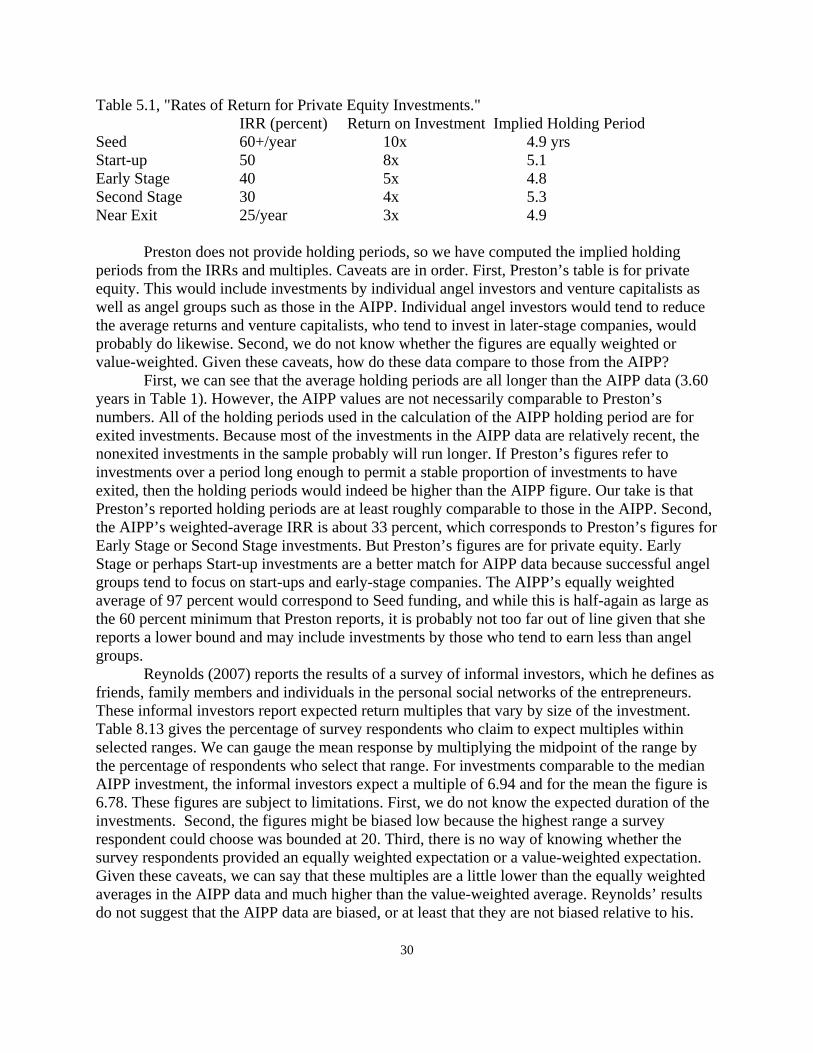
available estimates of expected returns come from surveys, and most focus on investment multiples or internal rates of return. Still, we can compare some of those values to those from our data. If the AIPP data are comparable to what others report, then we can probably conclude that any bias is small – or at least, no worse than any bias in the other data sources. We begin with base multiples and IRRs. The equally weighted average of the base multiples in our sample of 603 investments is 8.31. This means that the average project returns 8.31 times the total amount invested in the projects. Of course, non exited projects have returned little or nothing so far, so the equally weighted average of the 434 exited projects is higher -- 11.54. The average investment period is 3.6 years. This implies an IRR of 97 percent for the exited projects -- again, equally weighted. How does this compare to what others have reported? Shane (2009, p. 193) says that, "Given the failure rate of angel investments, successful angels target a thirty times multiple on their invested capital in five years.” A multiple of 30 over a five-year period implies an IRR of 97.4 percent, which is remarkably close to the 97 percent IRR in our data. This does beg the questions of whether or not the survey respondents are answering a question that makes the two figures comparable, and whether the AIPP respondents are “successful angels” or whether they are more or less “successful.” There is no way to know. Another question is whether respondents who said they expect an implied IRR of 97.4 percent meant that they expect individual investments to earn an average of 97.4 percent, or whether they meant that they expect the total return on all of their investments to be 97.4 percent. Put differently, did they report an equally weighted average or did they report a value-weighted average? The close correspondence between the AIPP’s implied IRR of 97 percent and the “successful angels’” implied IRR of 97.4 percent suggests that they reported an equally weighted average. Still, computing the comparable value-weighted average from the AIPP data is worthwhile. The value-weighted base multiple of the full sample of 603 investments is 2.24, which is a bit more than a quarter of the equally weighted average. For the 434 exited investments, the figure is 2.64, which is a bit less than a quarter of the equally weighted average. The value-weighted average for the years the investments were held is 3.39 (obtained by computing the total amount invested in each project, dividing by the total invested in all projects, multiplying each quotient by the years held, then summing the 434 results). The implied IRR in this case is only 33 percent, which is probably not too different from the expected returns on other risky equity portfolios during the sample period. This is especially true given that these 434 investments have all exited and probably will have done better than the nonexited investments in the AIPP, which would reduce the implied IRR. Based on these calculations derived from base multiples, we conclude that if the AIPP data are biased at all, then the bias does not appear to be extreme. What other numbers in the AIPP dataset can we compare? Preston (2007, page 92) gives IRRs and multiples for private equity. We reproduce Table 5.1 below:

30

Table 5.1, "Rates of Return for Private Equity Investments." IRR (percent) Return on Investment Implied Holding Period Seed 60+/year 10x 4.9 yrs Start-up 50 8x 5.1 Early Stage 40 5x 4.8 Second Stage 30 4x 5.3 Near Exit 25/year 3x 4.9 Preston does not provide holding periods, so we have computed the implied holding periods from the IRRs and multiples. Caveats are in order. First, Preston’s table is for private equity. This would include investments by individual angel investors and venture capitalists as well as angel groups such as those in the AIPP. Individual angel investors would tend to reduce the average returns and venture capitalists, who tend to invest in later-stage companies, would probably do likewise. Second, we do not know whether the figures are equally weighted or value-weighted. Given these caveats, how do these data compare to those from the AIPP? First, we can see that the average holding periods are all longer than the AIPP data (3.60 years in Table 1). However, the AIPP values are not necessarily comparable to Preston’s numbers. All of the holding periods used in the calculation of the AIPP holding period are for exited investments. Because most of the investments in the AIPP data are relatively recent, the nonexited investments in the sample probably will run longer. If Preston’s figures refer to investments over a period long enough to permit a stable proportion of investments to have exited, then the holding periods would indeed be higher than the AIPP figure. Our take is that Preston’s reported holding periods are at least roughly comparable to those in the AIPP. Second, the AIPP’s weighted-average IRR is about 33 percent, which corresponds to Preston’s figures for Early Stage or Second Stage investments. But Preston’s figures are for private equity. Early Stage or perhaps Start-up investments are a better match for AIPP data because successful angel groups tend to focus on start-ups and early-stage companies. The AIPP’s equally weighted average of 97 percent would correspond to Seed funding, and while this is half-again as large as the 60 percent minimum that Preston reports, it is probably not too far out of line given that she reports a lower bound and may include investments by those who tend to earn less than angel groups. Reynolds (2007) reports the results of a survey of informal investors, which he defines as friends, family members and individuals in the personal social networks of the entrepreneurs. These informal investors report expected return multiples that vary by size of the investment. Table 8.13 gives the percentage of survey respondents who claim to expect multiples within selected ranges. We can gauge the mean response by multiplying the midpoint of the range by the percentage of respondents who select that range. For investments comparable to the median AIPP investment, the informal investors expect a multiple of 6.94 and for the mean the figure is 6.78. These figures are subject to limitations. First, we do not know the expected duration of the investments. Second, the figures might be biased low because the highest range a survey respondent could choose was bounded at 20. Third, there is no way of knowing whether the survey respondents provided an equally weighted expectation or a value-weighted expectation. Given these caveats, we can say that these multiples are a little lower than the equally weighted averages in the AIPP data and much higher than the value-weighted average. Reynolds’ results do not suggest that the AIPP data are biased, or at least that they are not biased relative to his.

31

This is especially persuasive given that at least most of Reynolds’ informal investors are not members of groups and we know that such investors tend to earn less than angel groups. Additional information about expected returns can be gleaned from the information that angel groups provide to prospective entrepreneurs. For example, the website of Maine Angels, an angel group in Portland, ME (visited December 11, 2008), says that it typically funds between $100,000 and $2 million, and that, "Candidate companies should also have a high potential for growth and profitability, can provide at least 35% of annual return of investment within five to seven years and have a strategically planned and viable exit." All of the AIPP data are from a period before 2008, so to the extent that expectations shifted between the time of the investments in the AIPP projects and the end of 2008, these data may not be comparable. Still, the mean investment in the AIPP data is $154,730 (median $49,000), and 80 percent of the investments are between about $15,000 through about $300,000. Given that these figures are in nominal dollars, the AIPP data, being earlier, should be smaller, though not by enough to make these investment sizes comparable. A better explanation for the size disparity could be that the Maine Angels’ website may refer to the total investment by the entire group. The AIPP data are investments made by individual investors (though the individuals are members of a group). In short, the (individual) AIPP investments are smaller than the average Maine Angel group investment, and the value-weighted AIPP investment tends to return a bit less than the lower bound of Maine Angel’s expected amount (33 percent vs. 35 percent). Based on this, there is no evidence that the returns on the AIPP data are biased high. We can also compare the AIPP data on IPOs to those reported by other data sources. IPOs are the gold standard for angel investments, providing the extraordinarily high returns that catch the public’s eye. Band of Angels is perhaps the most famous angel group in the United States. According to Band of Angels’ website (visited March 1, 2009), Band of Angels has had nine IPOs out of 209 investments. This is only 4.3 percent. In contrast, the AIPP data have 57 IPOs out of 603 investments, or 9.5 percent. On the one hand, this is twice as high, but on the other hand, it is at least within an order of magnitude. Moreover, the fraction of buyouts – probably the second most profitable type of angel exit -- tilts the other way. Band of Angels has had 45 “profitable acquisitions,” or 21.5 percent of its investments exit via buyout while the corresponding AIPP figure is much lower, 14.4 percent (57/603). What does this tell us? It seems surprising that the investors in the AIPP would have a higher figure than Band of Angels, and this stands as the strongest evidence that the returns in the AIPP data are biased high. The much lower fraction of exits through buyouts, though, casts some doubt on the conclusion that the returns are biased high. Goldfarb, Hoberg, Kirsch and Triantis (2008, hereafter, GHKT) use the records of a failed law firm (Brobeck, Phleger & Harrison; hereafter, Brobeck). Unfortunately, their results are not directly comparable to the AIPP because GHKT include angel groups with venture capital firms. GHKT say that they conduct robustness checks and their main results are not sensitive to the way that they classify investments as venture capital, angel, founder or family. Still, this means that we cannot directly compare specific figures from GHKT's angel data with the AIPP data because the AIPP is from groups and GHKT bury their groups with venture deals. But neither can we compare the AIPP data with the GHKT’s venture capital results because those figures are dominated by venture capital deals. We can argue that GHKT’s angels, who are not members of groups, should be less successful than the investors in the AIPP (Shane, 2009). They probably conduct less due diligence and have lower returns than the investments in the AIPP data. This is especially true if some of Brobeck’s deals are loans rather than equity,

32

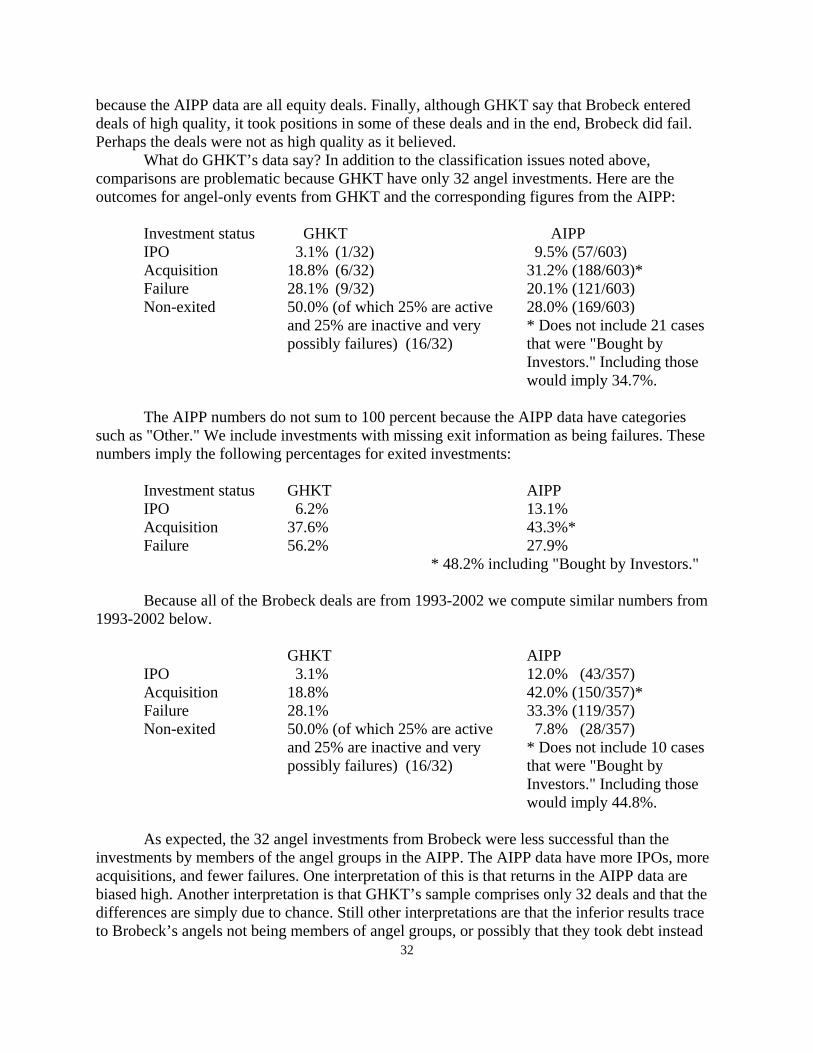
because the AIPP data are all equity deals. Finally, although GHKT say that Brobeck entered deals of high quality, it took positions in some of these deals and in the end, Brobeck did fail. Perhaps the deals were not as high quality as it believed. What do GHKT’s data say? In addition to the classification issues noted above, comparisons are problematic because GHKT have only 32 angel investments. Here are the outcomes for angel-only events from GHKT and the corresponding figures from the AIPP: Investment status GHKT AIPP IPO 3.1% (1/32) 9.5% (57/603) Acquisition 18.8% (6/32) 31.2% (188/603)* Failure 28.1% (9/32) 20.1% (121/603) Non-exited 50.0% (of which 25% are active 28.0% (169/603) and 25% are inactive and very * Does not include 21 cases possibly failures) (16/32) that were "Bought by Investors." Including those would imply 34.7%. The AIPP numbers do not sum to 100 percent because the AIPP data have categories such as "Other." We include investments with missing exit information as being failures. These numbers imply the following percentages for exited investments: Investment status GHKT AIPP IPO 6.2% 13.1% Acquisition 37.6% 43.3%* Failure 56.2% 27.9% * 48.2% including "Bought by Investors." Because all of the Brobeck deals are from 1993-2002 we compute similar numbers from 1993-2002 below. GHKT AIPP IPO 3.1% 12.0% (43/357) Acquisition 18.8% 42.0% (150/357)* Failure 28.1% 33.3% (119/357) Non-exited 50.0% (of which 25% are active 7.8% (28/357) and 25% are inactive and very * Does not include 10 cases possibly failures) (16/32) that were "Bought by Investors." Including those would imply 44.8%. As expected, the 32 angel investments from Brobeck were less successful than the investments by members of the angel groups in the AIPP. The AIPP data have more IPOs, more acquisitions, and fewer failures. One interpretation of this is that returns in the AIPP data are biased high. Another interpretation is that GHKT’s sample comprises only 32 deals and that the differences are simply due to chance. Still other interpretations are that the inferior results trace to Brobeck’s angels not being members of angel groups, or possibly that they took debt instead

33

of equity, or the deals were bad and contributed to the firm’s failure. If any of these is true, then the superior performance of the AIPP investors is unsurprising. We can also check whether the AIPP data are comparable to other data along dimensions other than returns. For example, GHKT (2008) says that about 18.8 percent of angels in angel-only deals had previously invested in the same company while Mason and Harrison (1996) report 25 percent. The percentage of investments with followon funding in the AIPP, which is 20.2 percent (122/603 deals), falls between these two figures. This suggests that the data in the AIPP are comparable at least along this dimension, and Cochran (2005) reports that venture capital investments that receive followon funding tend to have done well. If the AIPP data are biased, then we would expect them to have a higher proportion of followon investments. However, they do not. Unless the deals in GHKT or Mason and Harrison are biased, this stands as evidence that the AIPP data are relatively free of bias. The number of coinvestors provides another avenue by which to gain insight. Investments made with a coinvestor are probably less prone to bias because the survey respondent is more likely to be caught reporting biased results. There is, after all, at least one other person who knows about the project (even if he invests different amounts or at different times). In our data this comparison is problematic because there are many missing values for coinvestors. Still, it is worth doing. We find that t-tests show that the base multiple is insignificantly different between investments with coinvestors and those without. The same is true for annual multiples. When we regress the base multiple on the number of coinvestors, though, we obtain a significantly negative coefficient (-0.49, t-ratio = -2.44). This is consistent with selection bias in the data, which is being mitigated on deals with many coinvestors because the survey respondents are more likely to be caught reporting false data. This evidence of bias vanishes with annual multiples, though; the estimated coefficient (statistically insignificant) even reverses sign. This suggests that the regression is simply measuring the relation between the number of coinvestors and the duration of projects rather than between the number of coinvestors and the total return multiple. We also have deal size. It seems reasonable that larger deals are more likely to be remembered correctly. This alone would not eliminate intentional bias, but it would tend to eliminate unconscious bias. People may still lie, but they are less likely to remember only the good deals if the deals are large. Goldfarb, Hoberg, Kirsch and Triantis (2008) suggest that more sophisticated investors are more likely to do larger deals, too. Arguably, these sophisticated investors are less biased, or perhaps more likely to fear posting inflated results on the AIPP surveys but smaller figures on, say, their tax returns. To check this, we compute multiples on investments that are larger than the median and compare them with investments smaller than the median. The results show very marginal significance, with investments below the median having higher multiples. Although this is consistent with bias, the evidence is tenuous. In fact, after allowing for the statistically different variances between the groups, the p-value rises above 0.05. The significant result traces to three very small investments with huge multiples. Two investments of $1000 have base multiples of approximately 704 and 1333, and one investment of $10,000 had a base multiple of 900. The combines investment in these three projects is only about 8 percent of the mean investment in a single project. If we delete these three tiny observations, then the results do not even approach conventional significance levels. For annual multiples the results are similar but even less supportive of bias. None of the tests using annual multiples reveals a statistically significant difference between large and small investments.

34

Summary What then, does the evidence say regarding bias in the AIPP data? Based on the high percentage of investments that resulted in an IPO, we conclude that the data probably do contain some biases that inflate the reported performance of the angel groups that participated in the AIPP. However, the evidence of bias is hardly overwhelming. First, the fraction of sales tilts the other way. Second, implied internal rates of return and return multiples are comparable with figures from other sources, especially on a value-weighted basis. Finally, the data survive several checks designed to detect bias. The percentage of followon investments in the AIPP data, which are correlated with higher returns at least on venture deals, lies between comparable figures that other researchers report. Multiples from deals that are larger than the median do not differ statistically from those that are smaller than the median, and only one test using the number of coinvestors supports the claim that the returns data are biased high. Even if the AIPP data are free of bias, this does not mean that they are representative of angel investments in general. This is because the angel groups which participated in the study are far from representative of all angel investors. Aside from the advantages that members of groups enjoy, the types of investments differ. For example, Shane (2009) reports that many angel investments are debt, whereas all of the deals in the AIPP are equity. Angel investors who are members of groups tend to fare much better than those who are not.

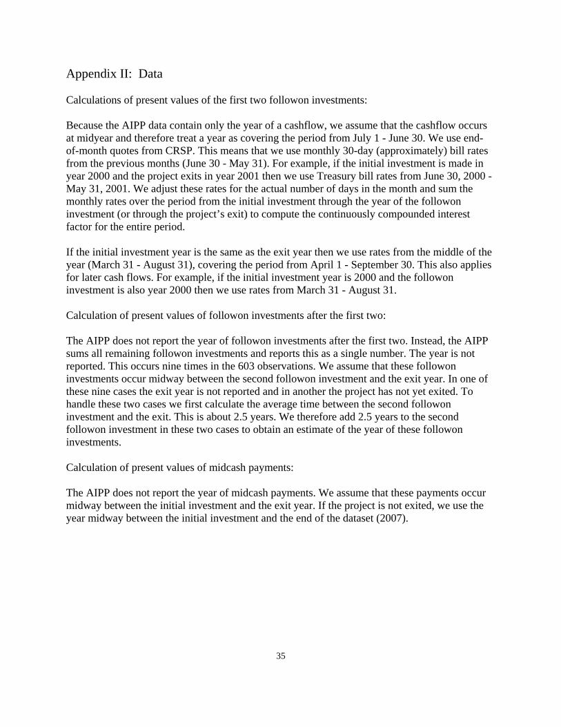
35

Appendix II: Data Calculations of present values of the first two followon investments: Because the AIPP data contain only the year of a cashflow, we assume that the cashflow occurs at midyear and therefore treat a year as covering the period from July 1 - June 30. We use end-of-month quotes from CRSP. This means that we use monthly 30-day (approximately) bill rates from the previous months (June 30 - May 31). For example, if the initial investment is made in year 2000 and the project exits in year 2001 then we use Treasury bill rates from June 30, 2000 - May 31, 2001. We adjust these rates for the actual number of days in the month and sum the monthly rates over the period from the initial investment through the year of the followon investment (or through the project’s exit) to compute the continuously compounded interest factor for the entire period. If the initial investment year is the same as the exit year then we use rates from the middle of the year (March 31 - August 31), covering the period from April 1 - September 30. This also applies for later cash flows. For example, if the initial investment year is 2000 and the followon investment is also year 2000 then we use rates from March 31 - August 31. Calculation of present values of followon investments after the first two: The AIPP does not report the year of followon investments after the first two. Instead, the AIPP sums all remaining followon investments and reports this as a single number. The year is not reported. This occurs nine times in the 603 observations. We assume that these followon investments occur midway between the second followon investment and the exit year. In one of these nine cases the exit year is not reported and in another the project has not yet exited. To handle these two cases we first calculate the average time between the second followon investment and the exit. This is about 2.5 years. We therefore add 2.5 years to the second followon investment in these two cases to obtain an estimate of the year of these followon investments. Calculation of present values of midcash payments: The AIPP does not report the year of midcash payments. We assume that these payments occur midway between the initial investment and the exit year. If the project is not exited, we use the year midway between the initial investment and the end of the dataset (2007).

36

Table 1

Sample Statistics

Number nonmissing Mean Median Standard

Deviation Minimum Maximum

Total Invested ($) 603 154,730 49,000 424,006 1000 5,100,000Total Cash Out ($) 430 477,486 40,833 2,169,970 0 33,000,000Base Multiple (X) Full sample 603 8.31 0 73.44 0 1332.8 Exited only 434 11.54 0.97 86.38 0 1332.8PV Base Multiple (X) Full Sample 603 8.34 0 73.46 0 1332.8 Exited only 434 11.59 0.97 86.40 0 1332.8Annual Multiple (X) Full Sample 603 2.29 0 20.91 0 480 Exited only 434 3.18 0.26 24.60 0 480PV Annual Multiple (X) Full Sample 603 2.29 0 20.91 0 480 Exited only 434 3.18 0.26 24.60 0 480Years Held 424 3.60 3.0 3.21 0.5 35Years Invested 306 11.33 8.0 9.97 1 49Years Entrepreneur 265 14.30 13.0 10.30 0 49Years Experience 252 5.81 0 9.68 0 47Number Companies 265 2.89 2.0 3.66 0 23Years Worked Large 263 13.70 12.0 10.78 0 40Total Investments 351 16.11 9.0 19.21 1 63Total Exits 377 6.97 2.0 12.94 0 42Total Wealth Held (%) 248 13.21 10.0 15.71 1 90Diligence (hours) 243 65.51 15.0 338.65 0 5000

Total Invested Total dollar amount invested in a specific project. Total Cash Out Total dollar amount returned by a specific project. Base Multiple Total cash returned divided by total cash invested. We treat the four exited

investments with missing exitcash as having returned zero. PV Base Multiple Similar to Base Multiple except that the followon investments and

midcash payments, if any, are discounted by netting out the riskless rate. Annual Multiple Base Multiple divided by Years Held. PV Annual Multiple PV Base Multiple divided by Years Held. Years Held Years between the angel investor’s initial investment in the venture and

exit from the venture. If the holding period is less than a year, then we treat the holding period as 0.5 years.

Years Invested Years that the angel investor has been investing.

37

Years Entrepreneur Years that the angel investor has been an entrepreneur. Years Experience Years of work experience the angel investor has in industries related to

this venture. Number Companies Number of firms the angel investor has founded. Years Worked Large Angel investor’s years of work experience in firms with more than 500

employees. Total Investments Total number of angel investments that the respondent has made. Total Exits Total number of angel investment exits that the respondent has

experienced. Total Wealth Held Percentage of angel’s personal wealth held in angel investments. Diligence Number of hours due diligence the angel investor conducted prior to

making the investment. Note: Of the 603 observations, 434 are exited investments and 169 are nonexited.

38

Table 2

Distribution of Base Multiples

Base Multiple Range 0 0.01-1.0

1.01-2.0

2.01-5.0

5.01-20.0 >20.0 Total

Number within Range 139 87 34 111 40 23 434 PV Base Multiple Range 0 0.01-

1.0 1.01-2.0

2.01-5.0

5.01-20.0 >20.0 Total

Number within Range 139 84 37 111 40 23 434 Base Multiples are the total dollar amount that the project returns divided by the total dollar amount invested in the project. The table includes only data for exited projects. A total of 434 projects have been exited and 169 have not yet been exited. In this table we treat five observations with all inflows as zero or missing as having returned nothing. PV Base Multiples are similar to Base Multiples except that the followon investments and midcash payments, if any, are discounted by netting out the riskless rate.

Table 3

Education Level of Angel Investors in the AIPP

Bachelors Masters JD Ph.D. Other Number Missing

Number Nonmissing

(Total Number) Number 71 168 19 29 10 306 297 (603) Highest degree attained by angel investors who reported this information. Of the 603 observations, 434 projects have been exited and 169 have not yet been exited.

39

Table 4

Exit Data

Exit Type

Ceased Operation

Bought by Another

Firm

Bought by

Investors IPO Other Number

Missing

Number Nonmissing

(Total) Number 121 188 21 57 10 37 397 (434)

The table contains the reasons given for exiting projects in the Angel Investor Performance Project dataset. We report data for only exited investments in this table (434 projects).

Table 5 Expected Returns

2*(0) (1 )*exp( .5 )nR p p μ σ= + − + (0.2)

Total observations

Observations with missing

data

Observations with

nonmissing data

Average annual log

return

Annual standard deviation

Estimate of expected annual

gross (net) returns

284 96 188 -0.0701 1.943 407% (307%)

281* 96 185 -0.1434 1.870 328% (228%) The table contains estimates of expected returns for projects with a single cash investment and a single (possibly zero) cash inflow. We estimate the probability of a zero cash inflow p as the number of observations with zero returns divided by the total number of observations (here, this equals 96/284 or 33.8 percent). * This line of the table reports results after dropping three very small investments (total of $12,000, which is less than 8 percent of the mean of a single investment) with extremely high returns (base multiples between 700 and 1333).

40

Table 6

i i i i iAdjYears Held Inityear VCinvestment Binaryfollowonα β γ δ ε= + + + + (0.3)

Variable Estimated coefficient

(t-ratio)

Constant 747.40 (12.53)**

Inityear -0.37 (-13.47) **

VCinvestment 0.72 (2.51)*

Binaryfollowon 0.97 (3.11)**

The sample is all 424 exited investments. Adjusted R-Square = 0.3071. * indicates significance at the 5% level. F-value = 63.50** ** indicates significance at the 1% level.

Table 7

i i i i iBaseMultiple Years Held Inityear Binaryfollowonα β γ δ ε= + + + + (0.4)

Variable Estimated coefficient

(t-ratio)

Constant 7120.25 (3.57)**

Years Held 6.00 (4.08) **

Inityear -3.56 (3.58)*

Binaryfollowon -13.91 (-1.49)

The sample is all 424 exited investments. Adjusted R-Square = 0.1288. * indicates significance at the 5% level. F-value = 21.85** ** indicates significance at the 1% level.

41

Table 8 Expected Returns

2*(0) (1 )*exp( .5 )nR p p μ σ= + − + (0.2)

Total observations

Observations with missing

data

Observations with

nonmissing data

Average annual log

return

Annual standard deviation

Estimate of expected annual

gross (net) returns

603 15 588 -0.3388 1.710 158% (58%) The table contains estimates of expected returns for projects. For exited projects we use annual multiples calculated from the AIPP data. For nonexited projects we compute estimates of the projects’ duration and use these to estimate annual returns. See the text for details. We estimate the probability of a zero cash inflow p as the number of observations with zero returns divided by the total number of observations (here, this equals 48.7 percent).

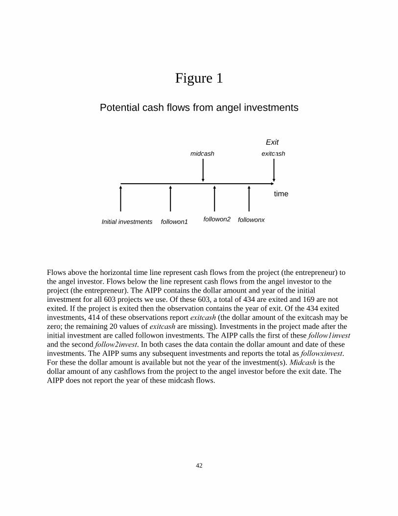
42

Figure 1

Potential cash flows from angel investments

Exitmidcash exitcash

time

Initial investments followon1 followon2 followonx

Flows above the horizontal time line represent cash flows from the project (the entrepreneur) to the angel investor. Flows below the line represent cash flows from the angel investor to the project (the entrepreneur). The AIPP contains the dollar amount and year of the initial investment for all 603 projects we use. Of these 603, a total of 434 are exited and 169 are not exited. If the project is exited then the observation contains the year of exit. Of the 434 exited investments, 414 of these observations report exitcash (the dollar amount of the exitcash may be zero; the remaining 20 values of exitcash are missing). Investments in the project made after the initial investment are called followon investments. The AIPP calls the first of these follow1invest and the second follow2invest. In both cases the data contain the dollar amount and date of these investments. The AIPP sums any subsequent investments and reports the total as followxinvest. For these the dollar amount is available but not the year of the investment(s). Midcash is the dollar amount of any cashflows from the project to the angel investor before the exit date. The AIPP does not report the year of these midcash flows.

43

Number of projects

The distribution of BaseMutiple, which is the total cash received divided by the total cash invested. Figure 2 uses all exited projects with usable data. A very small number of projects with huge returns distort the scale.

44

Number of projects

The distribution of BaseMutiple, which is the total cash received divided by the total cash invested. Figure 3 uses all exited projects with usable data and with gross returns less than or equal to 10 times the investment.