1

32nd International North Sea Flow Measurement Workshop 21-24 October 2014

Expanded Knowledge on Orifice Meter Response to Wet Gas Flows

Richard Steven, Colorado Engineering Experiment Station Inc. Josh Kinney, Colorado Engineering Experiment Station Inc.

Babajide Adejuyigbe, BP Exploration Operating Company, Ltd. Kim Lewis, DP Diagnostics LLC

1. INTRODUCTION

With orifice plate flow meters being one of the most widely used flow meters in the natural gas production industry it is inevitable that they are often used in wet natural gas flow applications. In 2011 BP, ConocoPhillips (CoP) and CEESI released a comprehensive paper (Steven et al [1]) on the known performance of the orifice meter to wet gas flow conditions. This paper described the performance of 2” through 4” orifice meters across a wide range of wet natural gas flow conditions. However, as with all gas meter types, there are still significant unknowns regards the performance of orifice meters with wet gas flow. In this paper three of these unknowns are addressed:

• The public knowledge of orifice meter wet gas performance includes an understanding of gas with a light hydrocarbon liquid and / or water. In this paper a rare 4”, 0.683 beta ratio orifice meter data set is discussed that includes the effects of wax in the hydrocarbon liquid and / or MEG being present.

• The publicly available orifice meter wet gas flow data set is largely confined to the nominal diameter (Ф) range 2”≤ Ф ≤ 4”. In this paper massed CEESI 8” orifice meter multiphase wet gas flow data is discussed.

• Orifice meter wet gas correction factors require the liquid flow rate be supplied from an external source. Traditionally the liquid flow rate is metered by periodic spot check techniques. An unnoticed change in the liquid flow rate between such checks induces a gas flow rate prediction bias. A real time qualitative liquid loading monitoring system is therefore useful. In this paper the DP meter diagnostic system ‘Prognosis’ (e.g. Skelton [2]) is analysed with wet gas orifice meter data to investigate its on line liquid loading monitoring capability.

2 THE DEFINITION OF WET GAS FLOW PARAMETERS

In this paper a wet gas flow is defined to be any two-phase (liquid and gas) flow where the Lockhart-Martinelli parameter (XLM) is less or equal to 0.3, i.e. XLM ≤ 0.3. This definition covers any combination of gaseous and liquid components. That is, the liquid can be a liquid hydrocarbon, water or a mix of liquid hydrocarbon and water. Other liquids and substances such as MEG / methanol, wax etc. may also be present.

l

g

g

totall

LM

m

mX

ρρ

.

,

.

= --- (1)

The Lockhart-Martinelli parameter (equation 1) is a non-dimensional expression

of the relative amount of liquid with the gas. Note that gm.

& totallm ,

.

are the gas

and liquid mass flow rates respectively (where totallm ,

.

is the sum of the individual

2

liquid component flows), while ρg & ρl are the average bulk gas and liquid

densities respectively.

The gas to liquid density ratio ( lgDR ρρ= ) is a non-dimensional expression of

pressure. The gas densiometric Froude numbers (gFr ), shown as equation 2, is a

non-dimensional expressions of the gas flow rate. Note that ‘g’ is the gravitational constant, ‘D’ is the meter inlet diameter and ‘A’ is the meter inlet cross sectional area.

( )glg

g

ggDA

mFr

ρρρ −= 1

.

---- (2)

With one single liquid component a wet gas has one liquid density. With multiphase wet gas flow there is two (or more) liquid densities. In this case the liquid density used to calculate the gas to liquid density ratio and the gas densiometric Froude number is the average liquid density.

“Water cut” is the ratio of the water to total liquid volume flow rates when the fluid is at standard conditions. In this paper “water to liquid mass ratio” (or ‘WLRm’) is defined as the ratio of the water mass flow rate to total liquid mass flow rates. As this paper discusses mixtures of water, hydrocarbon liquid and

MEG, the WLRm is calculated here by equation 3, where wm.

, hclm.

& MEGm.

are the

mass flow rates of water, hydrocarbon liquid and MEG respectively.

MEGhclw

w

m

mmm

mWLR

...

.

++= --- (3)

It is common engineering assumption to consider the liquid components

homogenously mixed. The homogenous liquid phase density ( hom,lρ ) is calculated

by equation 4, where wρ , hclρ and MEGρ are the water, hydrocarbon liquid and

MEG densities1 respectively. For multiphase wet gas flows it is this liquid mixture density that is used to calculate the wet gas flow parameters.

+

+

=MEGHCLwhclMEGwwMEGhcl

whclwtotall

l

mmm

m

...

,

.

hom,

ρρρρρρ

ρρρρ --- (4)

Equation 5 shows the orifice meter single phase gas mass flow equation. E & At are the velocity of approach and minimum cross sectional area respectively (both geometric constants), dC is the discharge coefficient, ε is expansibility and ∆Pg is

the traditionally read differential pressure (DP). The liquid induced gas flow rate prediction error is often called an “over-reading”, denoted here as “OR”. The traditional DP read when the flow is wet (∆Ptp) is different to that which would be read if that gas flowed alone (∆Pg). The result is an erroneous, or “apparent”, gas

mass flow rate prediction, apparentgm.

(see Equation 5a). Note that apparentgm.

, tpε

and tpdC , are the apparent (incorrect) gas mass flow rate prediction, the gas

1 The authors consider wet gas flow fluid properties to be information supplied to the flow computer from external means. Fluid property information is assumed to be correct. Whereas this is standard practice when discussing multiphase / wet gas flow metering, it is recognized that the supply of accurate fluid properties in field applications is a difficult challenge for operators.

3

ggdtg PCEAm ∆= ρε 2.

--- (5) tpgtpdtptapparentg PCEAm ∆= ρε 2,

.

--- (5a)

g

tp

g

tp

d

tpdtp

g

Apparentg

P

P

P

P

C

C

m

mOR

∆∆

≅∆∆

==ε

ε ,

.

.

--- (6)

%100*1%100*1%.

.

−

∆∆

≅

−=g

tp

g

Apparentg

P

P

m

mOR --- (6a)

expansibility and the discharge coefficient found respectively when applying the

wet gas differential pressure. (For many flow conditions εε dtptpd CC ≈, .) The over-

reading is expressed either as a ratio (equation 6) or percentage (equation 6a) comparison of the apparent to actual gas mass flow rate. Correction of this over-reading is the basis for orifice meter wet gas correlations. 3. ORIFICE METER MULTIPHASE WET GAS FLOW CORRECTION FACTOR

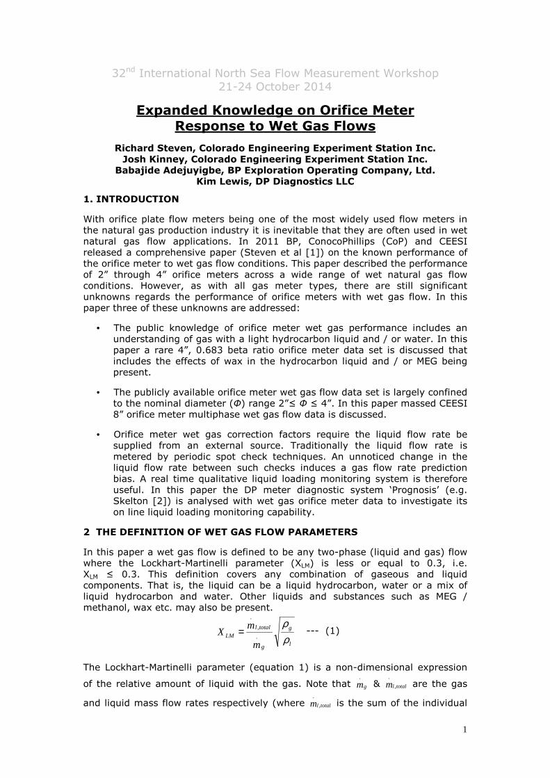
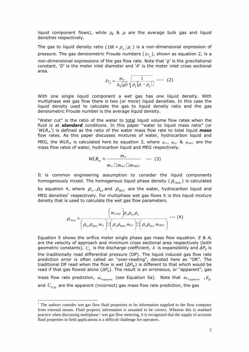
By 2011 CEESI, BP and CoP had gathered a massed orifice meter wet gas flow data set (of the range 2” ≤ D ≤ 4”) from multiple owners, tested at different facilities over many years. Figures 1, 2 & 3 show some of the orifice meters under test.

Fig 1. 2” Orifice Meter at CEESI Fig 2. 4” Orifice Meter at TUVNEL 2” multiphase wet gas flow facility. 4” two phase wet gas flow facility.

Fig 3. 4” Orifice Meter at CEESI 4” multiphase wet gas flow facility.

4

2

,

..

1 LMLM

apparentgg

XCX

mm

++= --- (7)

n

g

l

n

l

gC

+

=

ρρ

ρρ

--- (8)

( )mtransitiong WLRFr *2.05.1 += -- (9)

( )( ){ }mWLRA −−+= exp*1.04.0# -- (10)

2

,

#

2

1

−

=transitiong

stratFr

An -- (11)

stratnn = for transitiongg FrFr ,≤ -- (12a)

2

#

2

1

−

=gFr

An for transitiongg FrFr ,> -- (12b)

Note that ∞→Frg then 21→n as required

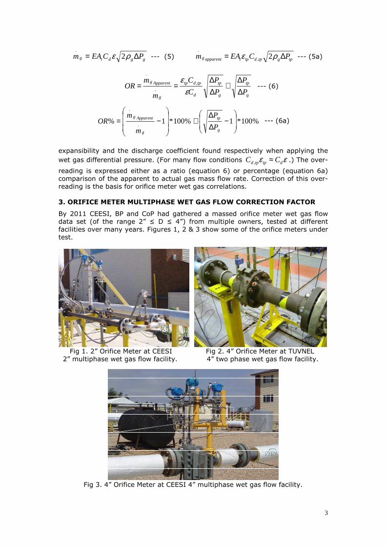
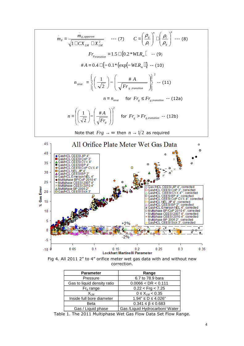
Fig 4. All 2011 2” to 4” orifice meter wet gas data with and without new

correction.

Parameter Range Pressure 6.7 to 78.9 bara

Gas to liquid density ratio 0.0066 < DR < 0.111 Frg range 0.22 < Frg < 7.25

XLM 0 ≤ XLM < 0.35 Inside full bore diameter 1.94” ≤ D ≤ 4.026”

Beta 0.341 ≤ β ≤ 0.683 Gas / Liquid phase Gas /Liquid Hydrocarbon/ Water

Table 1. The 2011 Multiphase Wet Gas Flow Data Set Flow Range.

5

Table 1 shows the range of the 2011 data set. Not all the maximum or minimum parameters were tested together. Analysis of this massed data set of 1656 wet gas flow points led to a 2” to 4” orifice meter wet gas correction factor reproduced here as equation set 7 through 12b. Figure 4 shows both this uncorrected data, and the data corrected for known liquid flow rates. For precisely known liquid flow rate inputs this correction factor has a 2% uncertainty to 95% confidence.

4. A UNIQUE 4”, 0.683β ORIFICE METER WET GAS FLOW DATA SET

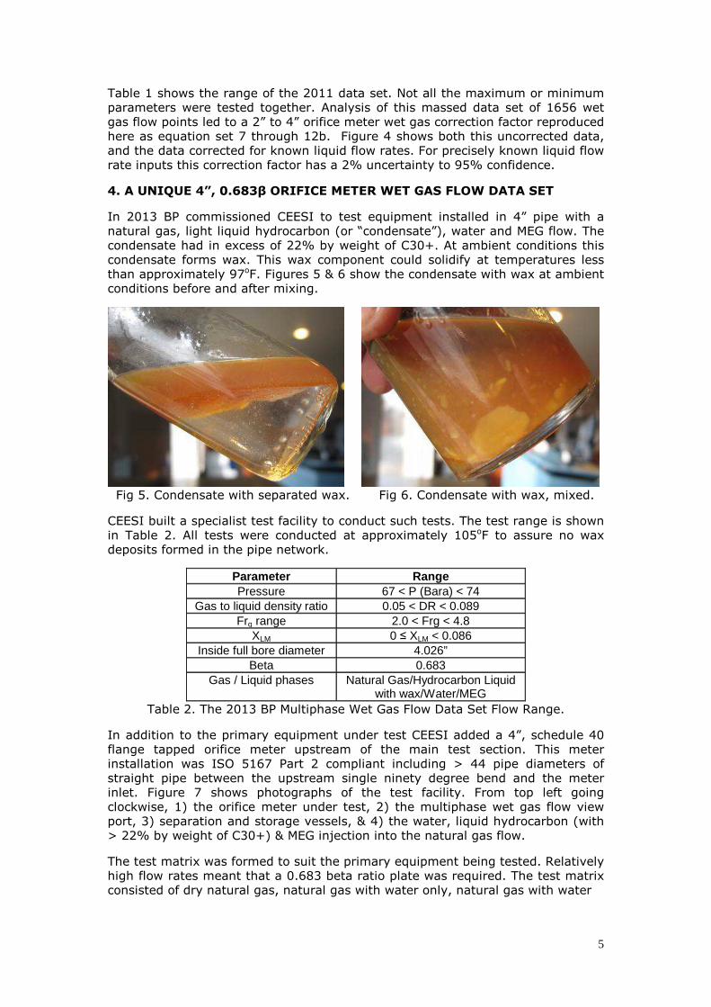
In 2013 BP commissioned CEESI to test equipment installed in 4” pipe with a natural gas, light liquid hydrocarbon (or “condensate”), water and MEG flow. The condensate had in excess of 22% by weight of C30+. At ambient conditions this condensate forms wax. This wax component could solidify at temperatures less than approximately 97oF. Figures 5 & 6 show the condensate with wax at ambient conditions before and after mixing.

Fig 5. Condensate with separated wax. Fig 6. Condensate with wax, mixed.

CEESI built a specialist test facility to conduct such tests. The test range is shown in Table 2. All tests were conducted at approximately 105oF to assure no wax deposits formed in the pipe network.

Parameter Range Pressure 67 < P (Bara) < 74

Gas to liquid density ratio 0.05 < DR < 0.089 Frg range 2.0 < Frg < 4.8

XLM 0 ≤ XLM < 0.086 Inside full bore diameter 4.026”

Beta 0.683 Gas / Liquid phases Natural Gas/Hydrocarbon Liquid

with wax/Water/MEG Table 2. The 2013 BP Multiphase Wet Gas Flow Data Set Flow Range.

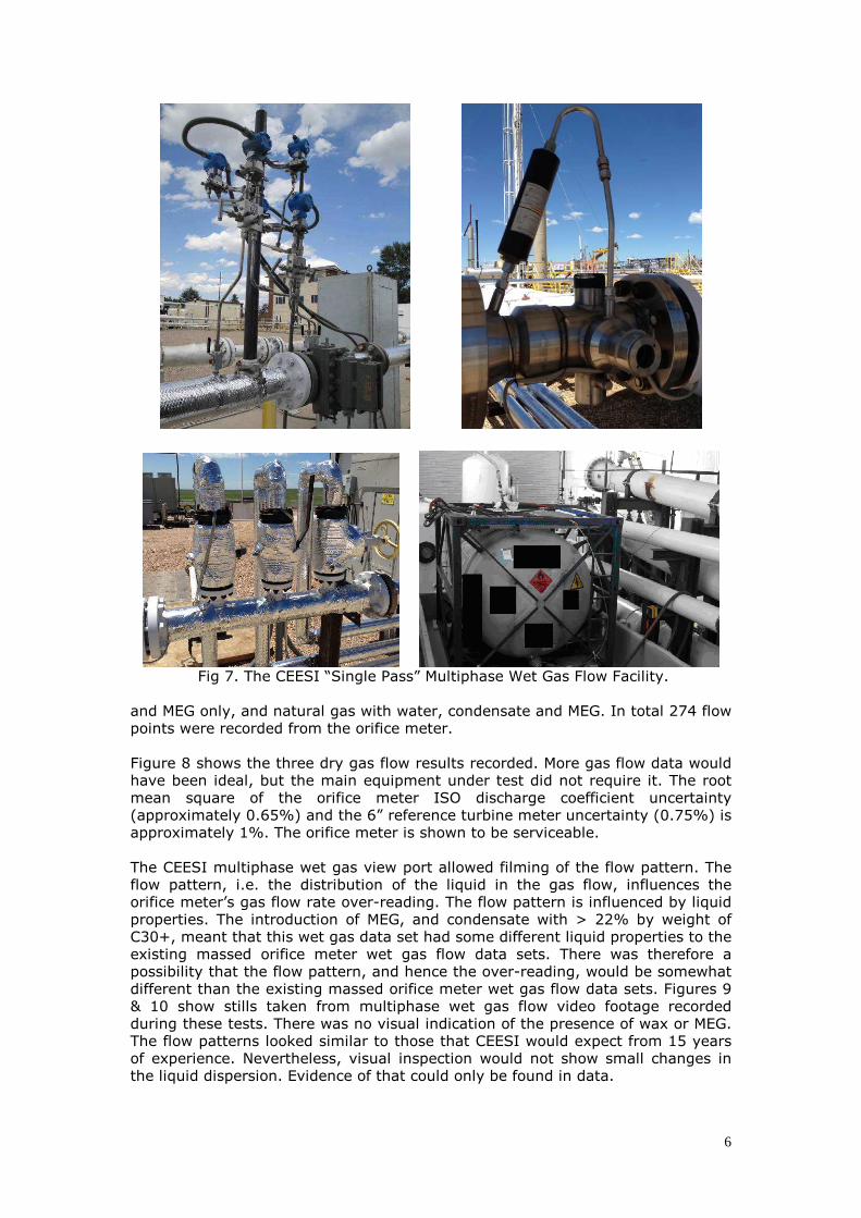
In addition to the primary equipment under test CEESI added a 4”, schedule 40 flange tapped orifice meter upstream of the main test section. This meter installation was ISO 5167 Part 2 compliant including > 44 pipe diameters of straight pipe between the upstream single ninety degree bend and the meter inlet. Figure 7 shows photographs of the test facility. From top left going clockwise, 1) the orifice meter under test, 2) the multiphase wet gas flow view port, 3) separation and storage vessels, & 4) the water, liquid hydrocarbon (with > 22% by weight of C30+) & MEG injection into the natural gas flow.

The test matrix was formed to suit the primary equipment being tested. Relatively high flow rates meant that a 0.683 beta ratio plate was required. The test matrix consisted of dry natural gas, natural gas with water only, natural gas with water

6

Fig 7. The CEESI “Single Pass” Multiphase Wet Gas Flow Facility.

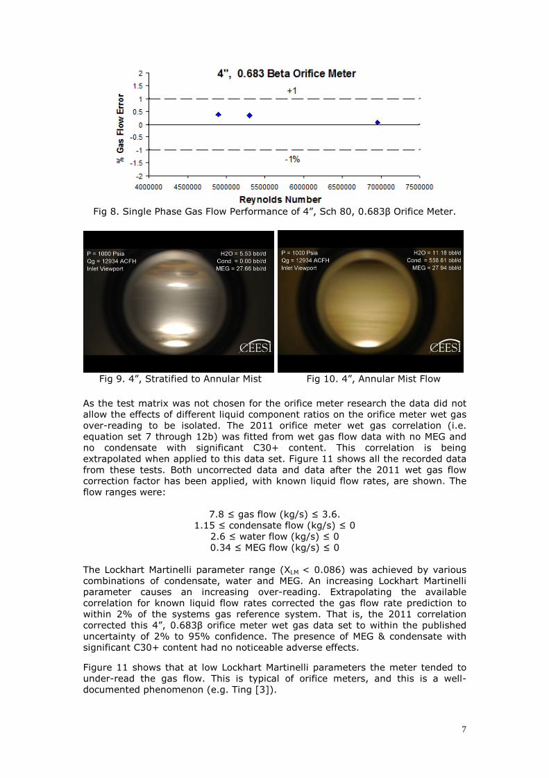
and MEG only, and natural gas with water, condensate and MEG. In total 274 flow points were recorded from the orifice meter. Figure 8 shows the three dry gas flow results recorded. More gas flow data would have been ideal, but the main equipment under test did not require it. The root mean square of the orifice meter ISO discharge coefficient uncertainty (approximately 0.65%) and the 6” reference turbine meter uncertainty (0.75%) is approximately 1%. The orifice meter is shown to be serviceable. The CEESI multiphase wet gas view port allowed filming of the flow pattern. The flow pattern, i.e. the distribution of the liquid in the gas flow, influences the orifice meter’s gas flow rate over-reading. The flow pattern is influenced by liquid properties. The introduction of MEG, and condensate with > 22% by weight of C30+, meant that this wet gas data set had some different liquid properties to the existing massed orifice meter wet gas flow data sets. There was therefore a possibility that the flow pattern, and hence the over-reading, would be somewhat different than the existing massed orifice meter wet gas flow data sets. Figures 9 & 10 show stills taken from multiphase wet gas flow video footage recorded during these tests. There was no visual indication of the presence of wax or MEG. The flow patterns looked similar to those that CEESI would expect from 15 years of experience. Nevertheless, visual inspection would not show small changes in the liquid dispersion. Evidence of that could only be found in data.

7

Fig 8. Single Phase Gas Flow Performance of 4”, Sch 80, 0.683β Orifice Meter.

Fig 9. 4”, Stratified to Annular Mist Fig 10. 4”, Annular Mist Flow

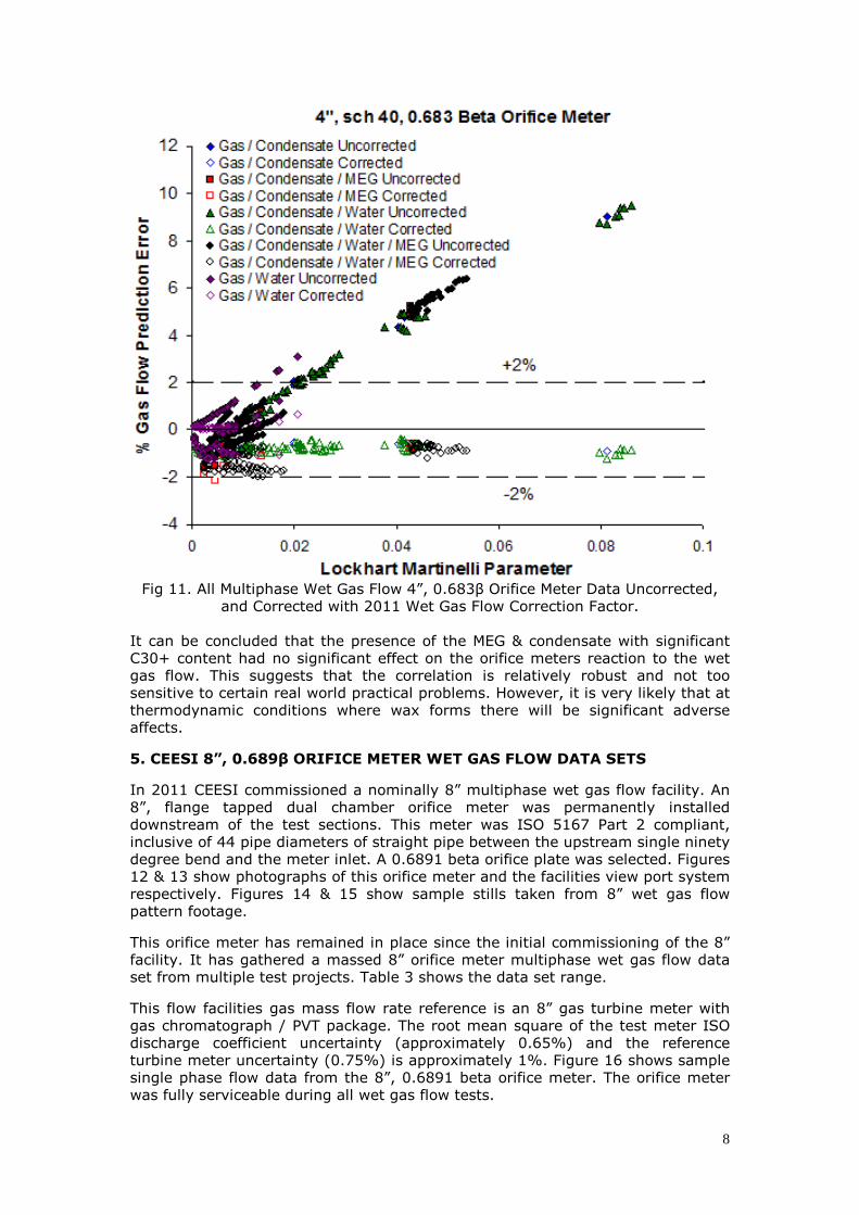
As the test matrix was not chosen for the orifice meter research the data did not allow the effects of different liquid component ratios on the orifice meter wet gas over-reading to be isolated. The 2011 orifice meter wet gas correlation (i.e. equation set 7 through 12b) was fitted from wet gas flow data with no MEG and no condensate with significant C30+ content. This correlation is being extrapolated when applied to this data set. Figure 11 shows all the recorded data from these tests. Both uncorrected data and data after the 2011 wet gas flow correction factor has been applied, with known liquid flow rates, are shown. The flow ranges were:

7.8 ≤ gas flow (kg/s) ≤ 3.6. 1.15 ≤ condensate flow (kg/s) ≤ 0

2.6 ≤ water flow (kg/s) ≤ 0 0.34 ≤ MEG flow (kg/s) ≤ 0

The Lockhart Martinelli parameter range (XLM < 0.086) was achieved by various combinations of condensate, water and MEG. An increasing Lockhart Martinelli parameter causes an increasing over-reading. Extrapolating the available correlation for known liquid flow rates corrected the gas flow rate prediction to within 2% of the systems gas reference system. That is, the 2011 correlation corrected this 4”, 0.683β orifice meter wet gas data set to within the published uncertainty of 2% to 95% confidence. The presence of MEG & condensate with significant C30+ content had no noticeable adverse effects.

Figure 11 shows that at low Lockhart Martinelli parameters the meter tended to under-read the gas flow. This is typical of orifice meters, and this is a well-documented phenomenon (e.g. Ting [3]).

8

Fig 11. All Multiphase Wet Gas Flow 4”, 0.683β Orifice Meter Data Uncorrected,

and Corrected with 2011 Wet Gas Flow Correction Factor. It can be concluded that the presence of the MEG & condensate with significant C30+ content had no significant effect on the orifice meters reaction to the wet gas flow. This suggests that the correlation is relatively robust and not too sensitive to certain real world practical problems. However, it is very likely that at thermodynamic conditions where wax forms there will be significant adverse affects.

5. CEESI 8”, 0.689β ORIFICE METER WET GAS FLOW DATA SETS

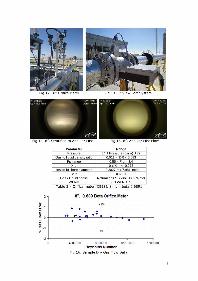
In 2011 CEESI commissioned a nominally 8” multiphase wet gas flow facility. An 8”, flange tapped dual chamber orifice meter was permanently installed downstream of the test sections. This meter was ISO 5167 Part 2 compliant, inclusive of 44 pipe diameters of straight pipe between the upstream single ninety degree bend and the meter inlet. A 0.6891 beta orifice plate was selected. Figures 12 & 13 show photographs of this orifice meter and the facilities view port system respectively. Figures 14 & 15 show sample stills taken from 8” wet gas flow pattern footage.

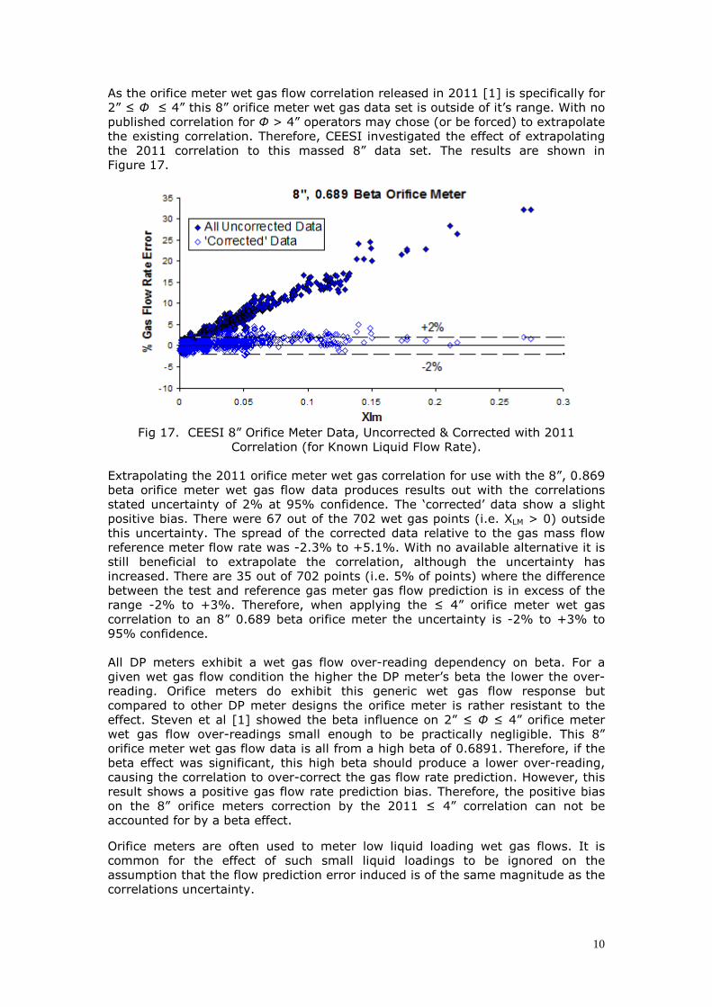
This orifice meter has remained in place since the initial commissioning of the 8” facility. It has gathered a massed 8” orifice meter multiphase wet gas flow data set from multiple test projects. Table 3 shows the data set range.

This flow facilities gas mass flow rate reference is an 8” gas turbine meter with gas chromatograph / PVT package. The root mean square of the test meter ISO discharge coefficient uncertainty (approximately 0.65%) and the reference turbine meter uncertainty (0.75%) is approximately 1%. Figure 16 shows sample single phase flow data from the 8”, 0.6891 beta orifice meter. The orifice meter was fully serviceable during all wet gas flow tests.

9

Fig 12. 8” Orifice Meter. Fig 13. 8” View Port System.

Fig 14. 8”, Stratified to Annular Mist Fig 15. 8”, Annular Mist Flow

Parameter Range Pressure 14 ≤ Pressure (bar a) ≤ 77

Gas to liquid density ratio 0.011 < DR < 0.083 Frg range 0.55 < Frg < 3.4

XLM 0 ≤ Xlm < 0.275 Inside full bore diameter 0.2027 m ( 7.981 inch)

Beta 0.6891 Gas / Liquid phase Natural gas / Exxsol D80 / Water

WLRm 0 ≤ WLR ≤ 1 Table 3 – Orifice meter, CEESI, 8 inch, beta 0.6891

Fig 16. Sample Dry Gas Flow Data.

10

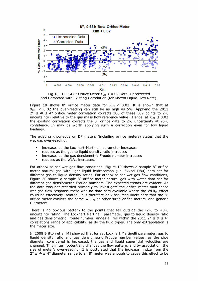
As the orifice meter wet gas flow correlation released in 2011 [1] is specifically for 2” ≤ Ф ≤ 4” this 8” orifice meter wet gas data set is outside of it’s range. With no published correlation for Ф > 4” operators may chose (or be forced) to extrapolate the existing correlation. Therefore, CEESI investigated the effect of extrapolating the 2011 correlation to this massed 8” data set. The results are shown in Figure 17.

Fig 17. CEESI 8” Orifice Meter Data, Uncorrected & Corrected with 2011

Correlation (for Known Liquid Flow Rate). Extrapolating the 2011 orifice meter wet gas correlation for use with the 8”, 0.869 beta orifice meter wet gas flow data produces results out with the correlations stated uncertainty of 2% at 95% confidence. The ‘corrected’ data show a slight positive bias. There were 67 out of the 702 wet gas points (i.e. XLM > 0) outside this uncertainty. The spread of the corrected data relative to the gas mass flow reference meter flow rate was -2.3% to +5.1%. With no available alternative it is still beneficial to extrapolate the correlation, although the uncertainty has increased. There are 35 out of 702 points (i.e. 5% of points) where the difference between the test and reference gas meter gas flow prediction is in excess of the range -2% to +3%. Therefore, when applying the ≤ 4” orifice meter wet gas correlation to an 8” 0.689 beta orifice meter the uncertainty is -2% to +3% to 95% confidence. All DP meters exhibit a wet gas flow over-reading dependency on beta. For a given wet gas flow condition the higher the DP meter’s beta the lower the over-reading. Orifice meters do exhibit this generic wet gas flow response but compared to other DP meter designs the orifice meter is rather resistant to the effect. Steven et al [1] showed the beta influence on 2” ≤ Ф ≤ 4” orifice meter wet gas flow over-readings small enough to be practically negligible. This 8” orifice meter wet gas flow data is all from a high beta of 0.6891. Therefore, if the beta effect was significant, this high beta should produce a lower over-reading, causing the correlation to over-correct the gas flow rate prediction. However, this result shows a positive gas flow rate prediction bias. Therefore, the positive bias on the 8” orifice meters correction by the 2011 ≤ 4” correlation can not be accounted for by a beta effect.

Orifice meters are often used to meter low liquid loading wet gas flows. It is common for the effect of such small liquid loadings to be ignored on the assumption that the flow prediction error induced is of the same magnitude as the correlations uncertainty.

11

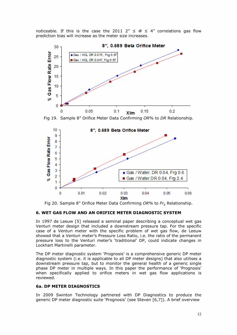
Fig 18. CEESI 8” Orifice Meter XLM < 0.02 Data, Uncorrected

and Corrected with Existing Correlation (for Known Liquid Flow Rate).

Figure 18 shows 8” orifice meter data for XLM < 0.02. It is shown that at XLM < 0.02 the over-reading can still be as high as 5%. Applying the 2011 2” ≤ Ф ≤ 4” orifice meter correlation corrects 306 of these 309 points to 2% uncertainty (relative to the gas mass flow reference value). Hence, at XLM ≤ 0.02 the existing correlation corrects the 8” orifice data to 2% uncertainty at 95% confidence. In may be worth applying such a correction even for low liquid loadings.

The existing knowledge on DP meters (including orifice meters) states that the wet gas over-reading:

• increases as the Lockhart-Martinelli parameter increases • reduces as the gas to liquid density ratio increases • increases as the gas densiometric Froude number increases • reduces as the WLRm increases.

For otherwise set wet gas flow conditions, Figure 19 shows a sample 8” orifice meter natural gas with light liquid hydrocarbon (i.e. Exxsol D80) data set for different gas to liquid density ratios. For otherwise set wet gas flow conditions, Figure 20 shows a sample 8” orifice meter natural gas with water data set for different gas densiometric Froude numbers. The expected trends are evident. As the data was not recorded primarily to investigate the orifice meter multiphase wet gas flow response there was no data sets available where the WLRm effect could be effectively isolated. It is therefore only assumed likely here that the 8” orifice meter exhibits the same WLRm as other sized orifice meters, and generic DP meters.

There is no obvious pattern to the points that fell outside the -2% to +3% uncertainty rating. The Lockhart Martinelli parameter, gas to liquid density ratio and gas densiometric Froude number ranges all fell within the 2011 2” ≤ Ф ≤ 4” correlations range of applicability, as do the fluid types. The only extrapolation is the meter size.

In 2008 Britton et al [4] showed that for set Lockhart Martinelli parameter, gas to liquid density ratio and gas densiometric Froude number values, as the pipe diameter considered is increased, the gas and liquid superficial velocities are changed. This in turn potentially changes the flow pattern, and by association, the size of meter’s over-reading. It is postulated that the increase in size from the 2” ≤ Ф ≤ 4” diameter range to an 8” meter was enough to cause this effect to be

12

noticeable. If this is the case the 2011 2” ≤ Ф ≤ 4” correlations gas flow prediction bias will increase as the meter size increases.

Fig 19. Sample 8” Orifice Meter Data Confirming OR% to DR Relationship.

Fig 20. Sample 8” Orifice Meter Data Confirming OR% to Frg Relationship.

6. WET GAS FLOW AND AN ORIFICE METER DIAGNOSTIC SYSTEM

In 1997 de Leeuw [5] released a seminal paper describing a conceptual wet gas Venturi meter design that included a downstream pressure tap. For the specific case of a Venturi meter with the specific problem of wet gas flow, de Leeuw showed that a Venturi meter’s Pressure Loss Ratio, i.e. the ratio of the permanent pressure loss to the Venturi meter’s ‘traditional’ DP, could indicate changes in Lockhart Martinelli parameter.

The DP meter diagnostic system ‘Prognosis’ is a comprehensive generic DP meter diagnostic system (i.e. it is applicable to all DP meter designs) that also utilises a downstream pressure tap, but to monitor the general health of a generic single phase DP meter in multiple ways. In this paper the performance of ‘Prognosis’ when specifically applied to orifice meters in wet gas flow applications is reviewed.

6a. DP METER DIAGNOSTICS

In 2009 Swinton Technology partnered with DP Diagnostics to produce the generic DP meter diagnostic suite ‘Prognosis’ (see Steven [6,7]). A brief overview

13

Fig 21. Orifice meter with instrumentation sketch and pressure fluctuation graph.

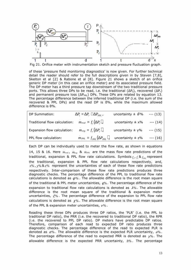
of these ‘pressure field monitoring diagnostics’ is now given. For further technical detail the reader should refer to the full descriptions given in by Steven [7,8], Skelton et al [2] & Rabone et al [8]. Figure 21 shows a sketch of an orifice generic DP meter (in this case an orifice meter) and its associated pressure field. The DP meter has a third pressure tap downstream of the two traditional pressure ports. This allows three DPs to be read, i.e. the traditional (∆Pt), recovered (∆Pr) and permanent pressure loss (∆PPPL) DPs. These DPs are related by equation 13. The percentage difference between the inferred traditional DP (i.e. the sum of the recovered & PPL DPs) and the read DP is δ%, while the maximum allowed difference is θ%.

DP Summation: PPLrt PPP ∆+∆=∆ , uncertainty ± θ % --- (13)

Traditional flow calculation: ( )tttrad Pfm ∆=.

, uncertainty ± x% --- (14)

Expansion flow calculation: ( )rr Pfm ∆=exp

.

, uncertainty ± y% --- (15)

PPL flow calculation: ( )PPLPPLPPL Pfm ∆=.

, uncertainty ± z% --- (16)

Each DP can be individually used to meter the flow rate, as shown in equations

14, 15 & 16. Here tradm.

, exp

.

m & PPLm.

are the mass flow rate predictions of the

traditional, expansion & PPL flow rate calculations. Symbolstf ,

rf &PPLf represent

the traditional, expansion & PPL flow rate calculations respectively, and,

%x , %y & %z represent the uncertainties of each of these flow rate predictions

respectively. Inter-comparison of these flow rate predictions produces three diagnostic checks. The percentage difference of the PPL to traditional flow rate calculations is denoted as %ψ . The allowable difference is the root mean square

of the traditional & PPL meter uncertainties, %φ . The percentage difference of the

expansion to traditional flow rate calculations is denoted as %λ . The allowable

difference is the root mean square of the traditional & expansion meter uncertainties, %ξ . The percentage difference of the expansion to PPL flow rate

calculations is denoted as %χ . The allowable difference is the root mean square

of the PPL & expansion meter uncertainties, %ν .

Reading these three DPs produces three DP ratios, the ‘PLR’ (i.e. the PPL to traditional DP ratio), the PRR (i.e. the recovered to traditional DP ratio), the RPR (i.e. the recovered to PPL DP ratio). DP meters have predictable DP ratios. Therefore, comparison of each read to expected DP ratio produces three diagnostic checks. The percentage difference of the read to expected PLR is denoted as %α . The allowable difference is the expected PLR uncertainty, %a .

The percentage difference of the read to expected PRR is denoted as %γ . The

allowable difference is the expected PRR uncertainty, %b . The percentage

14

difference of the read to expected RPR is denoted as %η . The allowable difference

is the expected RPR uncertainty, %c .

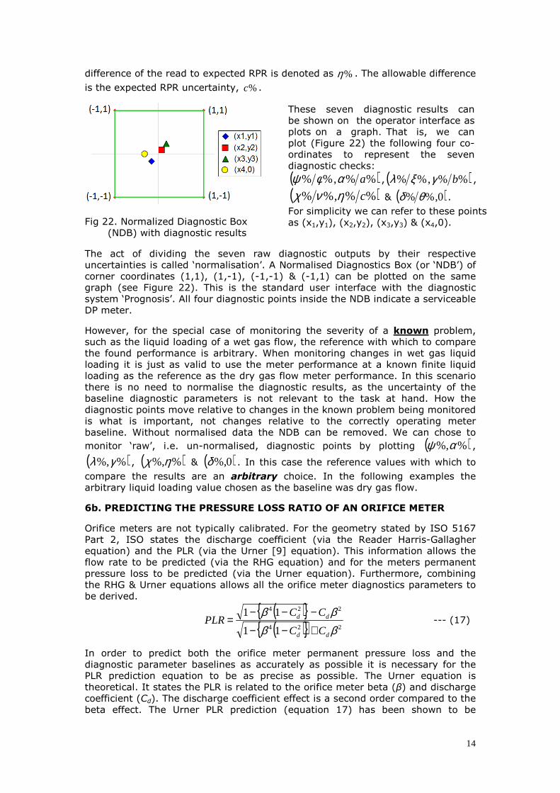
Fig 22. Normalized Diagnostic Box (NDB) with diagnostic results

These seven diagnostic results can be shown on the operator interface as plots on a graph. That is, we can plot (Figure 22) the following four co-ordinates to represent the seven diagnostic checks:

( )%%,%% aαφψ , ( )%%,%% bγξλ ,

( )%%,%% cηνχ & ( )0,%% θδ .

For simplicity we can refer to these points as (x1,y1), (x2,y2), (x3,y3) & (x4,0).

The act of dividing the seven raw diagnostic outputs by their respective uncertainties is called ‘normalisation’. A Normalised Diagnostics Box (or ‘NDB’) of corner coordinates (1,1), (1,-1), (-1,-1) & (-1,1) can be plotted on the same graph (see Figure 22). This is the standard user interface with the diagnostic system ‘Prognosis’. All four diagnostic points inside the NDB indicate a serviceable DP meter.

However, for the special case of monitoring the severity of a known problem, such as the liquid loading of a wet gas flow, the reference with which to compare the found performance is arbitrary. When monitoring changes in wet gas liquid loading it is just as valid to use the meter performance at a known finite liquid loading as the reference as the dry gas flow meter performance. In this scenario there is no need to normalise the diagnostic results, as the uncertainty of the baseline diagnostic parameters is not relevant to the task at hand. How the diagnostic points move relative to changes in the known problem being monitored is what is important, not changes relative to the correctly operating meter baseline. Without normalised data the NDB can be removed. We can chose to

monitor ‘raw’, i.e. un-normalised, diagnostic points by plotting ( )%%,αψ ,

( )%%,γλ , ( )%%,ηχ & ( )0%,δ . In this case the reference values with which to

compare the results are an arbitrary choice. In the following examples the arbitrary liquid loading value chosen as the baseline was dry gas flow.

6b. PREDICTING THE PRESSURE LOSS RATIO OF AN ORIFICE METER

Orifice meters are not typically calibrated. For the geometry stated by ISO 5167 Part 2, ISO states the discharge coefficient (via the Reader Harris-Gallagher equation) and the PLR (via the Urner [9] equation). This information allows the flow rate to be predicted (via the RHG equation) and for the meters permanent pressure loss to be predicted (via the Urner equation). Furthermore, combining the RHG & Urner equations allows all the orifice meter diagnostics parameters to be derived.

( ){ }( ){ } 224

224

11

11

ββββ

dd

dd

CC

CCPLR

+−−

−−−= --- (17)

In order to predict both the orifice meter permanent pressure loss and the diagnostic parameter baselines as accurately as possible it is necessary for the PLR prediction equation to be as precise as possible. The Urner equation is theoretical. It states the PLR is related to the orifice meter beta (β) and discharge coefficient (Cd). The discharge coefficient effect is a second order compared to the beta effect. The Urner PLR prediction (equation 17) has been shown to be

15

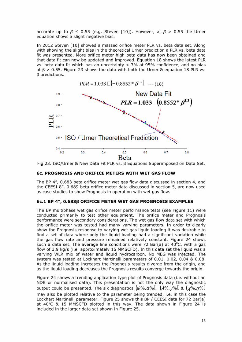
accurate up to β ≤ 0.55 (e.g. Steven [10]). However, at β > 0.55 the Urner equation shows a slight negative bias.

In 2012 Steven [10] showed a massed orifice meter PLR vs. beta data set. Along with showing the slight bias in the theoretical Urner prediction a PLR vs. beta data fit was presented. More orifice meter high beta data has now been obtained and that data fit can now be updated and improved. Equation 18 shows the latest PLR vs. beta data fit which has an uncertainty < 3% at 95% confidence, and no bias at β > 0.55. Figure 23 shows the data with both the Urner & equation 18 PLR vs. β predictions.

( )5.1*8552.0033.1 β−+=PLR --- (18)

Fig 23. ISO/Urner & New Data Fit PLR vs. β Equations Superimposed on Data Set. 6c. PROGNOSIS AND ORIFICE METERS WITH WET GAS FLOW

The BP 4”, 0.683 beta orifice meter wet gas flow data discussed in section 4, and the CEESI 8”, 0.689 beta orifice meter data discussed in section 5, are now used as case studies to show Prognosis in operation with wet gas flow. 6c.1 BP 4”, 0.683β ORIFICE METER WET GAS PROGNOSIS EXAMPLES

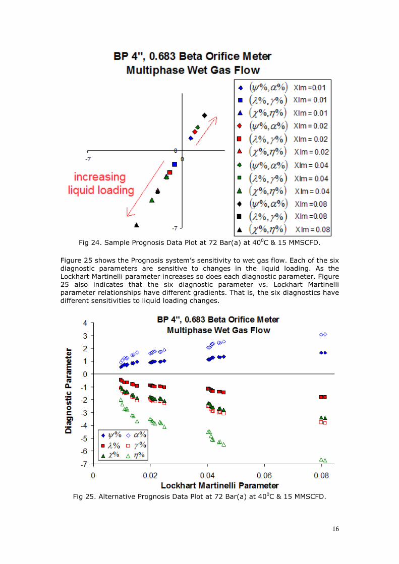
The BP multiphase wet gas orifice meter performance tests (see Figure 11) were conducted primarily to test other equipment. The orifice meter and Prognosis performance were secondary considerations. The wet gas flow data set with which the orifice meter was tested had many varying parameters. In order to clearly show the Prognosis response to varying wet gas liquid loading it was desirable to find a set of data where only the liquid loading had a significant variation while the gas flow rate and pressure remained relatively constant. Figure 24 shows such a data set. The average line conditions were 72 Bar(a) at 400C, with a gas flow of 3.9 kg/s (i.e. approximately 15 MMSCFD). In this data set the liquid was a varying WLR mix of water and liquid hydrocarbon. No MEG was injected. The system was tested at Lockhart Martinelli parameters of 0.01, 0.02, 0.04 & 0.08. As the liquid loading increases the Prognosis results diverge from the origin, and as the liquid loading decreases the Prognosis results converge towards the origin.

Figure 24 shows a trending application type plot of Prognosis data (i.e. without an NDB or normalised data). This presentation is not the only way the diagnostic

output could be presented. The six diagnostics ( )%%,αψ , ( )%%,γλ & ( )%%,ηχ

may also be plotted relative to the parameter being trended, i.e. in this case the Lockhart Martinelli parameter. Figure 25 shows this BP / CEESI data for 72 Bar(a) at 400C & 15 MMSCFD plotted in this way. The data shown in Figure 24 is included in the larger data set shown in Figure 25.

16

Fig 24. Sample Prognosis Data Plot at 72 Bar(a) at 400C & 15 MMSCFD.

Figure 25 shows the Prognosis system’s sensitivity to wet gas flow. Each of the six diagnostic parameters are sensitive to changes in the liquid loading. As the Lockhart Martinelli parameter increases so does each diagnostic parameter. Figure 25 also indicates that the six diagnostic parameter vs. Lockhart Martinelli parameter relationships have different gradients. That is, the six diagnostics have different sensitivities to liquid loading changes.

Fig 25. Alternative Prognosis Data Plot at 72 Bar(a) at 400C & 15 MMSCFD.

17

There are dedicated wet gas meter designs that use a Venturi meter in particular, coupled with the PLR vs. Lockhart Martinelli parameter in particular to make a wet gas liquid loading monitor. The PLR vs. Lockhart Martinelli parameter relationship

for this orifice meter is shown in Prognosis via %α . For the case of applying

Prognosis to orifice meters, whereas the parameter %α is clearly sensitive to

liquid loading, it is not the most sensitive, and therefore not the most useful of the orifice meter diagnostic parameters for monitoring liquid loading. The most sensitive, and therefore most useful of the orifice meter diagnostic parameters for

monitoring liquid loading are the DP ratios related to the recovered DP, i.e. %γ &

%η . These two parameters are not only more sensitive to small changes in

orifice meter liquid loading than the other parameters (including %α , i.e. the

PLR), but also continue to see changes in liquid loading until higher Lockhart Martinelli parameters, when the other parameters have gradually become insensitive to the increasing amounts of liquid. 6c.2 CEESI 8”, 0.683β ORIFICE METER WET GAS PROGNOSIS EXAMPLES

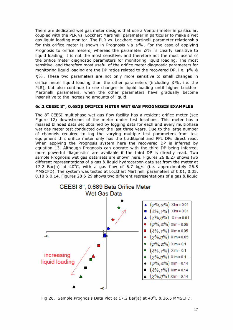
The 8” CEESI multiphase wet gas flow facility has a resident orifice meter (see Figure 12) downstream of the meter under test locations. This meter has a massed blinded data set obtained by logging data for each and every multiphase wet gas meter test conducted over the last three years. Due to the large number of channels required to log the varying multiple test parameters from test equipment this orifice meter only has the traditional and PPL DPs direct read. When applying the Prognosis system here the recovered DP is inferred by equation 13. Although Prognosis can operate with the third DP being inferred, more powerful diagnostics are available if the third DP is directly read. Two sample Prognosis wet gas data sets are shown here. Figures 26 & 27 shows two different representations of a gas & liquid hydrocarbon data set from the meter at 17.2 Bar(a) at 400C, with a gas flow of 6.7 kg/s (i.e. approximately 26.5 MMSCFD). The system was tested at Lockhart Martinelli parameters of 0.01, 0.05, 0.10 & 0.14. Figures 28 & 29 shows two different representations of a gas & liquid

Fig 26. Sample Prognosis Data Plot at 17.2 Bar(a) at 400C & 26.5 MMSCFD.

18

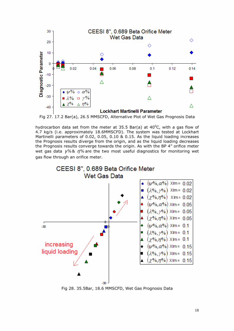
Fig 27. 17.2 Bar(a), 26.5 MMSCFD, Alternative Plot of Wet Gas Prognosis Data

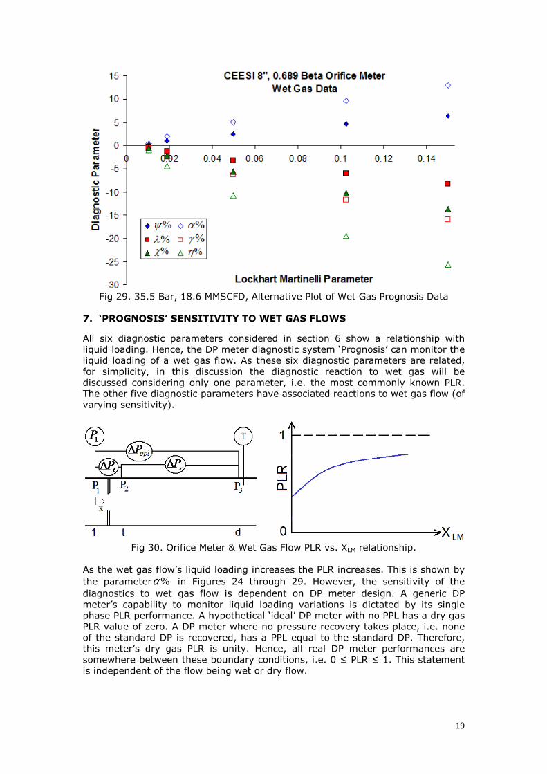
hydrocarbon data set from the meter at 35.5 Bar(a) at 400C, with a gas flow of 4.7 kg/s (i.e. approximately 18.6MMSCFD). The system was tested at Lockhart Martinelli parameters of 0.02, 0.05, 0.10 & 0.15. As the liquid loading increases the Prognosis results diverge from the origin, and as the liquid loading decreases the Prognosis results converge towards the origin. As with the BP 4” orifice meter

wet gas data %γ & %η are the two most useful diagnostics for monitoring wet

gas flow through an orifice meter.

Fig 28. 35.5Bar, 18.6 MMSCFD, Wet Gas Prognosis Data

19

Fig 29. 35.5 Bar, 18.6 MMSCFD, Alternative Plot of Wet Gas Prognosis Data

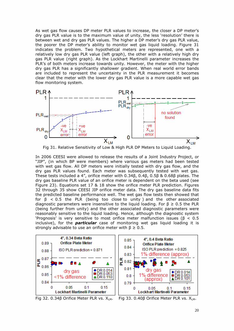
7. ‘PROGNOSIS’ SENSITIVITY TO WET GAS FLOWS

All six diagnostic parameters considered in section 6 show a relationship with liquid loading. Hence, the DP meter diagnostic system ‘Prognosis’ can monitor the liquid loading of a wet gas flow. As these six diagnostic parameters are related, for simplicity, in this discussion the diagnostic reaction to wet gas will be discussed considering only one parameter, i.e. the most commonly known PLR. The other five diagnostic parameters have associated reactions to wet gas flow (of varying sensitivity).

Fig 30. Orifice Meter & Wet Gas Flow PLR vs. XLM relationship.

As the wet gas flow’s liquid loading increases the PLR increases. This is shown by

the parameter %α in Figures 24 through 29. However, the sensitivity of the

diagnostics to wet gas flow is dependent on DP meter design. A generic DP meter’s capability to monitor liquid loading variations is dictated by its single phase PLR performance. A hypothetical ‘ideal’ DP meter with no PPL has a dry gas PLR value of zero. A DP meter where no pressure recovery takes place, i.e. none of the standard DP is recovered, has a PPL equal to the standard DP. Therefore, this meter’s dry gas PLR is unity. Hence, all real DP meter performances are somewhere between these boundary conditions, i.e. 0 ≤ PLR ≤ 1. This statement is independent of the flow being wet or dry flow.

20

As wet gas flow causes DP meter PLR values to increase, the closer a DP meter’s dry gas PLR value is to the maximum value of unity, the less ‘resolution’ there is between wet and dry gas PLR values. The higher a DP meter’s dry gas PLR value, the poorer the DP meter’s ability to monitor wet gas liquid loading. Figure 31 indicates the problem. Two hypothetical meters are represented, one with a relatively low dry gas PLR value (left graph), the other with a relatively high dry gas PLR value (right graph). As the Lockhart Martinelli parameter increases the PLR’s of both meters increase towards unity. However, the meter with the higher dry gas PLR has a significantly shallower gradient. When real world error bands are included to represent the uncertainty in the PLR measurement it becomes clear that the meter with the lower dry gas PLR value is a more capable wet gas flow monitoring system.

Fig 31. Relative Sensitivity of Low & High PLR DP Meters to Liquid Loading.

In 2006 CEESI were allowed to release the results of a Joint Industry Project, or “JIP”, (in which BP were members) where various gas meters had been tested with wet gas flow. All DP meters were initially tested with dry gas flow, and the dry gas PLR values found. Each meter was subsequently tested with wet gas. These tests included a 4”, orifice meter with 0.34β, 0.4β, 0.5β & 0.68β plates. The dry gas baseline PLR value of an orifice meter is dependent on the beta used (see Figure 23). Equations set 17 & 18 show the orifice meter PLR prediction. Figures 32 through 35 show CEESI JIP orifice meter data. The dry gas baseline data fits the predicted baseline performance well. The wet gas flow tests then showed that for β < 0.5 the PLR (being too close to unity ) and the other associated diagnostic parameters were insensitive to the liquid loading. For β ≥ 0.5 the PLR (being further from unity) and the other associated diagnostic parameters were reasonably sensitive to the liquid loading. Hence, although the diagnostic system ‘Prognosis’ is very sensitive to most orifice meter malfunction issues (β < 0.5 inclusive), for the particular case of monitoring wet gas liquid loading it is strongly advisable to use an orifice meter with β ≥ 0.5.

Fig 32. 0.34β Orifice Meter PLR vs. XLM. Fig 33. 0.40β Orifice Meter PLR vs. XLM.

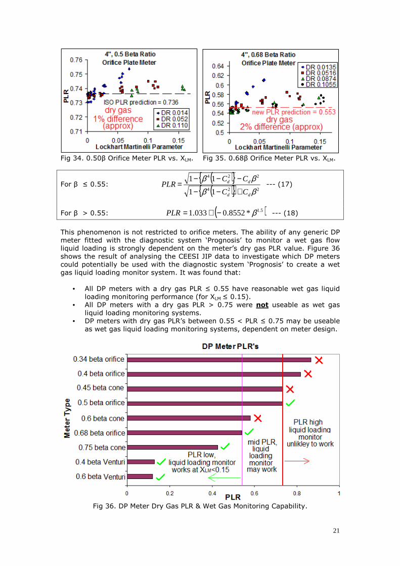
21

Fig 34. 0.50β Orifice Meter PLR vs. XLM. Fig 35. 0.68β Orifice Meter PLR vs. XLM.

For β ≤ 0.55: ( ){ }( ){ } 224

224

11

11

ββββ

dd

dd

CC

CCPLR

+−−

−−−= --- (17)

For β > 0.55: ( )5.1*8552.0033.1 β−+=PLR --- (18)

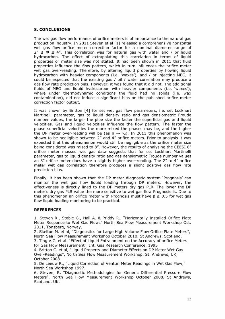
This phenomenon is not restricted to orifice meters. The ability of any generic DP meter fitted with the diagnostic system ‘Prognosis’ to monitor a wet gas flow liquid loading is strongly dependent on the meter’s dry gas PLR value. Figure 36 shows the result of analysing the CEESI JIP data to investigate which DP meters could potentially be used with the diagnostic system ‘Prognosis’ to create a wet gas liquid loading monitor system. It was found that:

• All DP meters with a dry gas PLR ≤ 0.55 have reasonable wet gas liquid loading monitoring performance (for XLM ≤ 0.15).

• All DP meters with a dry gas PLR > 0.75 were not useable as wet gas liquid loading monitoring systems.

• DP meters with dry gas PLR’s between 0.55 < PLR ≤ 0.75 may be useable as wet gas liquid loading monitoring systems, dependent on meter design.

Fig 36. DP Meter Dry Gas PLR & Wet Gas Monitoring Capability.

22

8. CONCLUSIONS The wet gas flow performance of orifice meters is of importance to the natural gas production industry. In 2011 Steven et al [1] released a comprehensive horizontal wet gas flow orifice meter correction factor for a nominal diameter range of 2” ≤ Ф ≤ 4”. This correlation was for natural gas with water and / or liquid hydrocarbon. The effect of extrapolating this correlation in terms of liquid properties or meter size was not stated. It had been shown in 2011 that fluid properties influence the flow pattern, which in turn influences the orifice meter wet gas over-reading. Therefore, by altering liquid properties by flowing liquid hydrocarbon with heavier components (i.e. ‘waxes’), and / or injecting MEG, it could be expected that the existing gas / oil / water correlation may produce a gas flow rate prediction bias. However, it was found that it did not. The additional fluids of MEG and liquid hydrocarbon with heavier components (i.e. ‘waxes’), where under thermodynamic conditions the fluid had no solids (i.e. wax contamination), did not induce a significant bias on the published orifice meter correction factor output.

It was shown by Britton [4] for set wet gas flow parameters, i.e. set Lockhart Martinelli parameter, gas to liquid density ratio and gas densiometric Froude number values, the larger the pipe size the faster the superficial gas and liquid velocities. Gas and liquid velocities influence the flow pattern. The faster the phase superficial velocities the more mixed the phases may be, and the higher the DP meter over-reading will be (as n → ½). In 2011 this phenomenon was

shown to be negligible between 2” and 4” orifice meters. Prior to analysis it was expected that this phenomenon would still be negligible as the orifice meter size being considered was raised to 8”. However, the results of analysing the CEESI 8” orifice meter massed wet gas data suggests that for set Lockhart Martinelli parameter, gas to liquid density ratio and gas densiometric Froude number values an 8” orifice meter does have a slightly higher over-reading. The 2” to 4” orifice meter wet gas correlation therefore produces a slight positive gas flow rate prediction bias.

Finally, it has been shown that the DP meter diagnostic system ‘Prognosis’ can monitor the wet gas flow liquid loading through DP meters. However, the effectiveness is directly lined to the DP meters dry gas PLR. The lower the DP meter’s dry gas PLR value the more sensitive to wet gas flow Prognosis is. Due to this phenomenon an orifice meter with Prognosis must have β ≥ 0.5 for wet gas flow liquid loading monitoring to be practical. REFERENCES

1. Steven R., Stobie G., Hall A. & Priddy R., “Horizontally Installed Orifice Plate Meter Response to Wet Gas Flows” North Sea Flow Measurement Workshop Oct. 2011, Tonsberg, Norway. 2. Skelton M. et al, “Diagnostics for Large High Volume Flow Orifice Plate Meters”, North Sea Flow Measurement Workshop October 2010, St Andrews, Scotland. 3. Ting V.C. et al. “Effect of Liquid Entrainment on the Accuracy of orifice Meters for Gas Flow Measurement”, Int. Gas Research Conference, 1995 4. Britton C. et al, “Liquid Property and Diameter Effects on DP Meter Wet Gas Over-Readings”, North Sea Flow Measurement Workshop, St. Andrews, UK, October 2008 5. De Leeuw R., "Liquid Correction of Venturi Meter Readings in Wet Gas Flow," North Sea Workshop 1997. 6. Steven, R. “Diagnostic Methodologies for Generic Differential Pressure Flow Meters”, North Sea Flow Measurement Workshop October 2008, St Andrews, Scotland, UK.

23

7. Steven, R. “Significantly Improved Capabilities of DP Meter Diagnostic Methodologies”, North Sea Flow Measurement Workshop October 2009, Tonsberg, Norway. 8. Rabone, “Operator Experience with DP Meter Diagnostics”, North Sea Flow Measurement Workshop Oct. 2012, St Andrews, Scotland. 9. Urner, G., “Pressure loss of orifice plates according to ISO 5167”, Flow Measurement and Instrumentation, 8, March 1997, pp. 39-41 10. Steven R. et al, “Differential Pressure Meters – A Cabinet of Curiosities (and Some Alternative Views on Accepted DP Meter Axioms)”, North Sea Flow Measurement Workshop Oct. 2012, St Andrews, Scotland.