Exit Polls, Turnout, and Bandwagon Voting:

Evidence from a Natural Experiment

Rebecca B. Morton, Daniel Muller, Lionel Page, and Benno Torgler∗

February 5, 2013

Abstract

We exploit a voting reform in France to estimate the causal effect of

exit poll information on turnout and bandwagon voting. Before the change

in legislation, individuals in some French overseas territories voted after

the election result had already been made public via exit poll information

from mainland France. We estimate that knowing the exit poll informa-

tion decreases voter turnout by about 12 percentage points. Our study is

the first clean empirical design outside of the laboratory to demonstrate

the effect of such knowledge on voter turnout. Furthermore, we find that

exit poll information significantly increases bandwagon voting; that is,

voters who choose to turn out are more likely to vote for the expected

winner.

∗Morton: Department of Politics, New York University (e-mail: rebecca.morton@nyu.edu).

Muller and Page: School of Economics and Finance, Queensland University of Technology

and QuBE (e-mail: d3.mueller@qut.edu.au and lionel.page@qut.edu.au). Torgler: School of

Economics and Finance, Queensland University of Technology and EBS Business School, ISBS,

EBS Universitat fur Wirtschaft und Recht and CREMA – Center for Research in Economics,

Management and the Arts and QuBE (e-mail: benno.torgler@qut.edu.au). We thank Pauline

Grosjean, Arye Hillman, Bjorn Kauder, Jeffrey M. Wooldridge and participants of the 5th

Australasian Public Choice Conference for helpful discussions and Malka Guillot for excellent

research assistance.

1

1 Introduction

“A Californian plans to vote after work in what she believes to be

a close presidential election. (She has little interest in the race for

congressman for her district, although it is closer.) The day is rainy

and as she approaches the polling place she sees a long line. On

the radio she hears that one presidential candidate has a substantial

lead in other states. She says why bother and turns her car around

and drives home.”

Sudman (1986, p. 332)

In August, 2009, exit poll results for key regional elections in Germany were

leaked on Twitter before voting ended. These polls showed that Chancellor

Angela Merkel’s conservative party had much less support than in previous

elections. Wolfgang Bosbach, deputy parliamentary head of Merkel’s Christian

Union bloc, said that the leaked results “damaged democracy” and a spokesman

for the pro-business Free Democrats, Merkel’s preferred coalition partner, com-

mented that the leaks were “unacceptable.” In addition, such reporting is

against the German law with a fine of up to 50,000 euros, so German election of-

ficials immediately began to investigate whether the Twitter messages violated

the law.1 The German case is not unusual: a survey of 66 countries world-

wide finds that of the 59 that permit exit polls during an election, 41 prohibit

publication of the results until after all voting has concluded (see Spangenberg

(2003)).

Yet in recent 21st century elections, incidents similar to the 2009 Twitter

controversy in Germany abound. In 2007, the websites of several Swiss and

Belgium newspapers crashed when French citizens attempted to access exit poll

results during an election and in the 2012 French presidential election, results

were also available online while voting was still in progress.2 Countries with

multiple time zones like France, the United States, Canada or Russia, in which

1See Carter (2009).2See Sayare (2012).

2

voting takes place at different times in different regions face particular difficul-

ties.3 The notorious reporting on Floridian exit poll results in the 2000 United

States presidential election occurred while voters in the western part of the

state and the rest of the nation were still voting. In 2004 leaked US presidential

exit poll results were commonly discussed among voters while east coast voters

were still going to the ballot booths.4 With the proliferation of Twitter, Face-

book, and other social media worldwide, the ability of governments to control

and limit leaked exit polls both inside and outside their countries is becoming

increasingly difficult.

Despite the growing tendency for voters to learn exit polls results while an

election is still ongoing, observational data-based research on the effects of such

information on voting behavior is limited and inconclusive. One possible natural

setting for exploring this issue is the so-called West Coast effect in the U.S.; that

is, the release of early East Coast election returns before the polls close on the

West Coast due to the fact that the presidential election takes place in three

different continental time zones. The debate over this effect emerged in the early

1960s after the introduction of sophisticated computer models, improved survey

techniques for predicting election results, and rapid access to media information.

The first set of related studies, however, which explored the 1964 presidential

election, showed barely any West Coast effect (see for example McAllister and

Studlar (1991)).

A second set of major studies focused on the 1980 election,5 in which pre-

election polls indicated a close election between Reagan and Carter, but Carter

3The United States does not prohibit the reporting of exit poll results, so elections are

often publicly decided before voters in Alaska and Hawaii have voted, and sometimes while

voting in California and other western states is still ongoing. In Canada polls close at the

same time across the country to reduce the potential of leaked results. In India, although the

country is not subject to the same time zone issues, voting is conducted at different times in

different regions for security reasons and reporting early results is illegal.4See Best and Krueger (2012) for a review.5It should be noted that other elections between 1964 and 1980 have also been explicitly

analyzed. For example, Tuchman and Coffin (1971) explore the influence of election night

television broadcasts on the close 1968 election but find no evidence that it affected voting.

3

conceded defeat even before the polls closed in the west.6 However, although

these researchers used a richer set of data (aggregated data on various elections,

regional, data or congressional districts, or better survey data), they produced

mixed results. For example, Jackson (1983), using a pool of 1981 persons inter-

viewed before and after the election, found some evidence that media coverage

of exit polls in the 1980 U.S. presidential election did lead to a reduction in

turnout. However, the survey data used in his and a number of similar studies

of the 2000 election have been strongly criticized as unreliable (see the review

in Frankovic (2001)7).

Despite this lack of conclusive observational evidence on exit polls’ effects

on subsequent voter choices, however, a few laboratory studies, do suggest that

information about early voting can have significant effects on voter behavior.

These studies indicate that later voters’ choices appear to be influenced by

information about early voting. More specifically, later voters with the same

preferences who have learned early voter choices make different turnout decisions

(see Battaglini, Morton, and Palfrey (2007)) or vote for different candidates (see

Hung and Plott (2001), Morton and Williams (1999) and Morton and Williams

(2001)) than they would have done without that information.

If, as the experimental evidence suggests, later voters are indeed so influ-

enced by early voting results, then the advent of increasing social media reports

6NBC was also strongly criticized for declaring Ronald Reagan the President of the United

States at 8:15PM eastern standard time based on its own computer projections: “Articles,

reports, and letters were written describing how voting lines outside polling places disappeared,

how turnout decreased over prior years, and how voters stayed home after it became apparent

that their favored candidates had already won or lost” (Leonardo (1983, p. 297)). Criticism

also emerged that national voter turnout decreased to 53.95% (the rate since 1948, see Dubois

(1983)). All this criticism led to a congressional hearing, journalistic commentary, private

studies, and a task force report, as well as the proposition of remedial bills to regulate either

poll closing times or the timing of network election predictions, but no action was taken once

interest began disappearing (Leonardo (1983), Carpini (1984)).7Frankovic, Kathleen, “Part Three: Historical Perspective,” in Linda Mason, Kathleen

Frankovic, and Kathleen Hall Jamieson, CBS News Coverage of Election Night 2000: Inves-

tigation, Analysis, Recommendations, January 2001.

4

of election results through exit polls can lead to fundamental changes in the

way voters behave. It may thus have important consequences for how democ-

racy works in many countries. Most obviously, candidates and political parties

may have incentives to manipulate the reported results in order to seek advan-

tages. But even if the results are accurately reported, other serious effects might

occur. For example, if later voters are less likely to participate or have a ten-

dency to engage in bandwagon voting, then the candidates preferred by earlier

voters may be more likely to win elections. To the extent that the timing of the

voter participation decision is exogenous and depends on voter characteristics

such as income, ethnicity or other factors that arguably affect voter preferences,

then voters may be unequally represented even though their votes are theo-

retically equal. At the same time, to the extent that the timing of voting is

endogenous, candidates and political parties will have an incentive to engage in

strategic manipulation of the factors that influence when individuals choose to

participate, much like the strategic manipulation in the timing of presidential

primaries in the United States.8 Hence, given that the election process is fun-

damentally changing with social media reporting of exit poll results, whether

later voters’ choices are influenced is an important empirical question for many

countries in which such information has historically not been available.9

In this paper, we make use of a unique natural experiment to address the

question whether later voters behavior is affected by exit poll information about

earlier voter choices. Specifically, we exploit a 2005 voting reform in France to

estimate the causal effect of exit poll information on turnout and bandwagon (or

underdog) voting. Before the change in legislation, individuals in French west-

ern overseas territories voted after the mainland election results were already

known via exit polls. This reform creates an exogenous variation in information

for a well identified group of voters and provides therefore the setting for a nat-

ural experiment to study the effect of exit poll information on voters behavior.

8See Morton and Williams (1999) for a discussion of these manipulations.9 Thompson (2004) presents additional normative and philosophical arguments against the

revelation of such information to later voters.

5

Such an approach has two advantages. First, relative to existing studies on the

West Coast effect, our natural experimental setting allows us to eliminate lots of

the possible caveats in the analysis of the causal effect of information by provid-

ing a counterfactual situation (same constituencies with and without exit poll

information). Second, our study does not suffer for the possible concern about

the ecological validity of the results, a criticism often raised about laboratory

experiments.

Using this voting reform to study the effect of exit poll information, we

find evidence that the public knowledge about such polls not only decreases

turnout by about 10 percentage points, but also increases bandwagon voting.

We therefore conclude that exit polls can indeed have consequential effects on

voter behavior and that the advent of social media reporting on exit poll in-

formation may fundamentally change the democratic process in many countries

where such information was previously unavailable.

In the next section, we review the relevant theoretical literature on informa-

tion and voting behavior. Section 3 then outlines our empirical research design

and the natural experiment, Section 4 presents our results regarding the effect

on turnout, Section 5 addresses robustness concerns and Section 6 presents the

results on the Bandwagon effect. We conclude and discuss the implications of

our analysis in Section 7.

2 The Role of Exit Poll Information in Voting

Choices: Theory and Experimental Evidence

When individuals know the results from earlier voting as in leaked exit polls,

voting becomes sequential in nature. In the case of complete information about

the choices before voters but incomplete information about other participants’

preferences, learning the results of earlier decisions simply provides later par-

ticipants with information about the likelihood that their vote may be pivotal.

It is thus straightforward to show that if voting is costly (even if the costs are

6

minimal), learning that one’s own decision will not affect the outcome implies

that a rational individual should abstain. If however, a voter learns instead that

the election is extremely close and the probability of being pivotal is high, then

later voters may actually participate at greater rates than they would if voting

were simultaneous and they had less precise information about other voter’s

choices.

If voters have private information about the choices before them in an elec-

tion, then early voting results not only reveal the extent to which individual

choice may be pivotal but may also provide later voters with insights into the

information held by early voters about the choices. As shown by Battaglini

(2005), when voting is costly the set of equilibria in sequential private infor-

mation voting games are disjoint from those in which voting is simultaneous.

That is, later voters’ choices will be influenced by the results of early voting.

Battaglini, Morton, and Palfrey (2007) also find support for these qualitative

theoretical predictions in laboratory elections using a three-voter game; in par-

ticular, they find significant evidence of strategic abstention by later voters.

Other results, however, are at variance with theory – they find that early voters

tend to participate more than theoretically predicted, whereas later voters ab-

stain more, sometimes even when their votes could be pivotal. They conclude

that, as predicted, although sequential voting tends to be more informationally

and economically efficient than simultaneous voting, later voters benefit at the

expense of early voters, so there is a cost in terms of equity. Nevertheless, they

find no evidence of later voters ignoring their private information and engaging

in bandwagon or underdog voting.

Callander (2007) considers the comparison of simultaneous and sequential

voting under asymmetric information when voters receive utility from conform-

ing to the majority (voting for the winner) independent of the utility they de-

rive from whether the winner is their own best choice. Specifically, he derives

an equilibrium under sequential voting in which voters engage in bandwagon

voting (voting for the leading candidate) even though their private information

may suggest that the leading candidate is not their own best choice. He finds

7

that such bandwagon voting may occur even when later voters’ choices are not

pivotal and the outcome is already decided (because of the additional utility

voters receive from the act of voting for the winning candidate). This argument

is supported by earlier work by Hung and Plott (2001), which provides experi-

mental evidence of conformity voting when subjects are rewarded for doing so.

Presumably, if voters similarly receive utility from voting for an underdog can-

didate (or are rewarded for doing so in an experiment), then later voters may

also engage in underdog voting even when they previously believed the leading

candidate to be their own best choice.

Hence, both theory and the experimental evidence suggests that if the act

of voting is costly, when later voters learn from exit poll information that their

decision is unlikely to be pivotal, they are more likely to abstain. If, however,

they receive utility from the act of voting for either the winner or the underdog

(independent of whether the winner is their own best choice), then such exit poll

information may lead them to engage in either bandwagon or underdog voting,

respectively.

Our natural experiment allows us to evaluate the extent to which exit poll

information affects the turnout of later voters and whether later voters are more

likely to engage in either bandwagon or underdog voting.

3 The Natural Experiment: Institutional Back-

ground and Empirical Strategy

3.1 The French Electoral System

France is one of the few countries in Europe to have a presidential system.

The French president is directly elected by the citizens via a two-round runoff

system. In the first round a large number of candidates can participate.10

If one candidate receives more than 50% of the votes in the first round he

10To be eligible to run, a candidate must gather 500 signatures from local politicians such

as town councilors.

8

or she is declared the winner. Such an immediate victory, however, has only

happened once since the beginning of the Fifth Republic, in 1958.11 Usually,

the two candidates that receive the most votes participate in a second round to

determine the winner.

This two-round runoff system model is also used in most other elections in

France with some variation. The French parliamentary elections differ slightly

in the sense that the two-round runoff elections within each constituency allow

more than two candidates to participate in the second round.12 In practice,

however, although a few second rounds are disputed by three candidates, most

involve only two.

Balloting traditionally takes place on a Sunday. French electoral law pro-

hibits exit poll publication until the close of voting in mainland France (Bale

(2002)) and bans publication, broadcasting and commenting on opinion polls

for the day before and the day of the election (Saturday and Sunday). The

electoral law also stipulates that the official campaign has to stop for these last

two days.13

When a French presidential election is held, it is always the only contest on

the ballot, which stands in contrast to, for example, U.S. elections, in which bal-

lots include local, congressional and senatorial posts, and even local propositions

and initiatives. The French case thus allows us to measure turnout for presi-

dential elections only, meaning that the turnout measured is not confounded by

effects from other elections.

During the day of the election, the release of exit polls is therefore not allowed

11This presidential election was the first one of the Fifth Republic. De Gaulle had overseen

the design of the new constitution and was seen as having saved France from a potential

military coup by the many army generals opposed to the process of Algerian independence.

In these dramatic circumstances, De Gaulle won the election with more than 78% of the votes.12In order to participate in the second round, candidates must gather a minimum proportion

of registered voters in the constituency, currently 12.5%. In presidential elections, however,

there are always exactly two candidates in the second round.13The law was initially voted in in 1977. At that time, the publication and broadcasting

of opinion polls were banned for one week before each of the two rounds of voting. It was

changed in 2002 to limit this interdiction to the last two days before the results.

9

until after the closure of the last polling booth in mainland France, on Sunday

at 8:00PM CET.14 At exactly 8:00PM, TV channels release highly precise early

estimations of the final results. These are based on large exit polls and on the

first results from the majority of polling booths, which close at 6:00PM.15

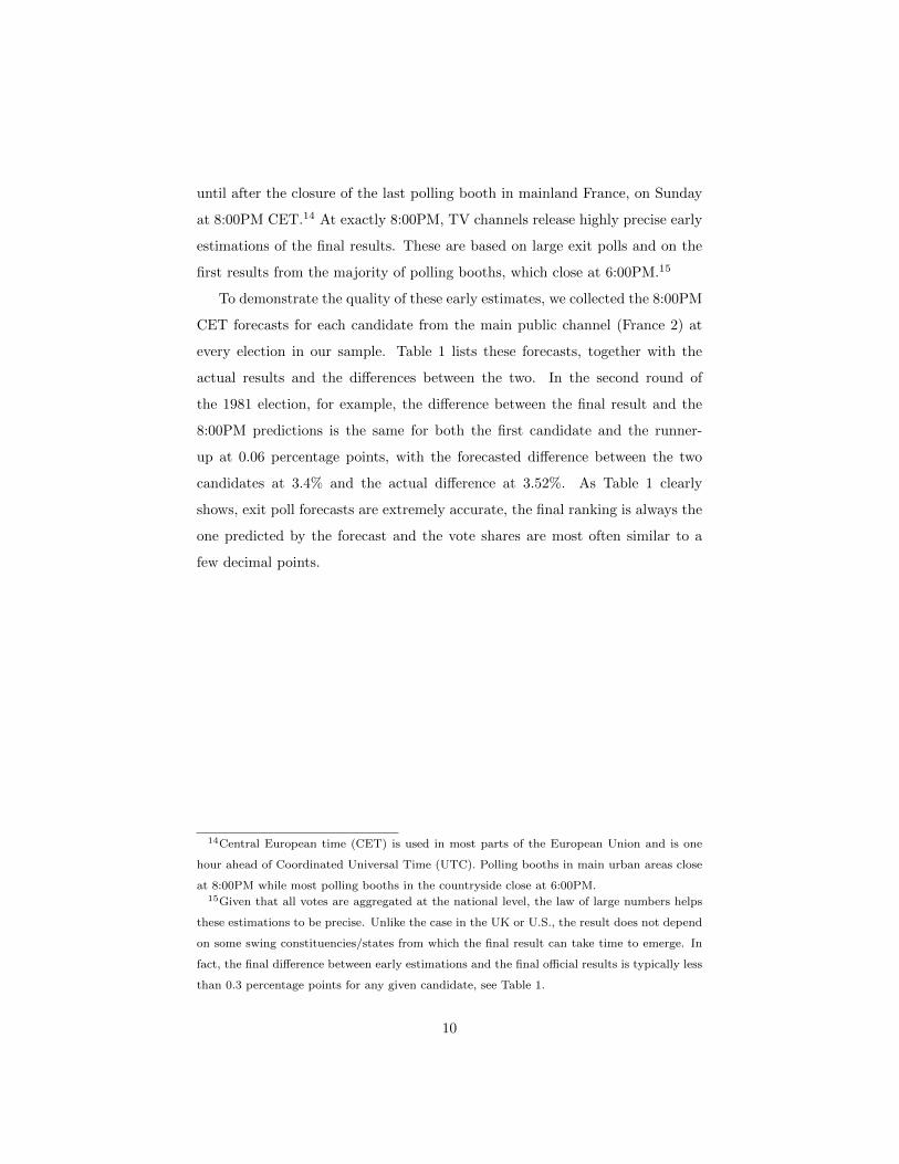
To demonstrate the quality of these early estimates, we collected the 8:00PM

CET forecasts for each candidate from the main public channel (France 2) at

every election in our sample. Table 1 lists these forecasts, together with the

actual results and the differences between the two. In the second round of

the 1981 election, for example, the difference between the final result and the

8:00PM predictions is the same for both the first candidate and the runner-

up at 0.06 percentage points, with the forecasted difference between the two

candidates at 3.4% and the actual difference at 3.52%. As Table 1 clearly

shows, exit poll forecasts are extremely accurate, the final ranking is always the

one predicted by the forecast and the vote shares are most often similar to a

few decimal points.

14Central European time (CET) is used in most parts of the European Union and is one

hour ahead of Coordinated Universal Time (UTC). Polling booths in main urban areas close

at 8:00PM while most polling booths in the countryside close at 6:00PM.15Given that all votes are aggregated at the national level, the law of large numbers helps

these estimations to be precise. Unlike the case in the UK or U.S., the result does not depend

on some swing constituencies/states from which the final result can take time to emerge. In

fact, the final difference between early estimations and the final official results is typically less

than 0.3 percentage points for any given candidate, see Table 1.

10

Fir

stca

nd

idat

eS

econ

dca

nd

idate

Th

ird

can

did

ate

Diff

piv

ota

lca

nd

idate

s

Yea

rR

oun

dF

orec

ast

Res

ult

Diff

Fore

cast

Res

ult

Diff

Fore

cast

Res

ult

Diff

Fore

cast

Res

ult

Diff

1981

128

.328

.32

-0.0

225.2

25.8

5-0

.65

17.9

18

-0.1

7.3

7.8

50.5

5

251

.751

.76

-0.0

648.3

48.2

40.0

6-

--

3.4

3.5

20.1

2

1988

134

.434

.10.3

019.5

19.9

4-0

.44

16.5

16.5

5-0

.05

33.3

90.3

9

253

.954

.02

-0.1

246.1

45.9

80.1

2-

--

7.8

8.0

40.2

4

1995

123

.423

.30.1

20

20.8

4-0

.84

18.5

18.5

8-0

.08

1.5

2.2

60.7

6

252

52.6

4-0

.64

48

47.3

60.6

4-

--

45.2

81.2

8

2002

120

19.8

80.1

21

17

16.8

60.1

416

16.1

8-0

.18

10.6

8-0

.32

282

.182

.21

-0.1

117.9

17.7

90.1

1-

--

64.2

64.4

20.2

2

2007

129

.631

.18

-1.5

825.1

25.8

7-0

.77

18.7

18.5

70.1

36.4

7.3

0.9

0

253

53.0

6-0

.06

47

46.9

40.0

6-

--

66.1

20.1

2

2012

128

.428

.63

-0.2

325.5

27.1

8-1

.68

20

17.9

2.1

5.5

9.2

83.7

8

251

.951

.64

0.2

648.1

48.3

6-0

.26

--

-3.8

03.2

8-0

.52

Tab

le1:

For

ecas

tsas

pre

sente

dby

Fra

nce

’sm

ain

pu

bli

cT

Vch

an

nel

Fra

nce

2at

8:0

0P

M.

All

nu

mb

ers

are

inp

erce

nta

ge

poin

ts.

“Piv

otal

can

did

ates

”re

fers

toth

efi

rst

an

dse

con

dca

nd

idate

inth

ese

con

dro

un

dan

dth

ese

con

dan

dth

eth

ird

can

did

ate

in

the

firs

tro

un

d.

11

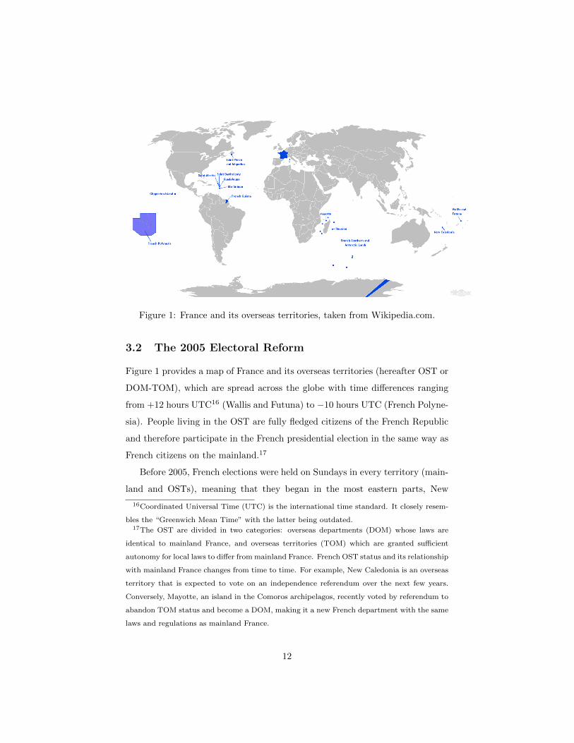
Figure 1: France and its overseas territories, taken from Wikipedia.com.

3.2 The 2005 Electoral Reform

Figure 1 provides a map of France and its overseas territories (hereafter OST or

DOM-TOM), which are spread across the globe with time differences ranging

from +12 hours UTC16 (Wallis and Futuna) to −10 hours UTC (French Polyne-

sia). People living in the OST are fully fledged citizens of the French Republic

and therefore participate in the French presidential election in the same way as

French citizens on the mainland.17

Before 2005, French elections were held on Sundays in every territory (main-

land and OSTs), meaning that they began in the most eastern parts, New

16Coordinated Universal Time (UTC) is the international time standard. It closely resem-

bles the “Greenwich Mean Time” with the latter being outdated.17The OST are divided in two categories: overseas departments (DOM) whose laws are

identical to mainland France, and overseas territories (TOM) which are granted sufficient

autonomy for local laws to differ from mainland France. French OST status and its relationship

with mainland France changes from time to time. For example, New Caledonia is an overseas

territory that is expected to vote on an independence referendum over the next few years.

Conversely, Mayotte, an island in the Comoros archipelagos, recently voted by referendum to

abandon TOM status and become a DOM, making it a new French department with the same

laws and regulations as mainland France.

12

Caledonia, Wallis and Futuna, and then moved progressively across the more

westerly territories as the opening time for polling booths arrived (typically be-

tween 8:00AM and 9:00AM). As a result, the territories located to the west of

the French mainland (e.g. the Caribbean, Guiana) and in the Pacific (French

Polynesia) voted partially or completely after mainland France.

Because the mainland accounts for approximately 96% of the total French

population,18 in national ballots like presidential elections, the result on the

mainland almost certainly determines the overall election result. This setting

is therefore different from that of the U.S., where the number of electoral votes

determined by California can empirically decide the outcome of a close contest.

Table 1 shows that in most cases the result is fully determined once the

mainland results are known. Voters in overseas territories west of mainland

France only represent around 1.5% of the French electorate. The predicted

difference between the two “pivotal candidates” (the first versus the runner-up

in the second round and the second versus the third candidate in the first round)

given by exit polls is almost always below 1.5%.

To illustrate this point further, Table 2 shows the number of votes by which

the runner-up was ahead of the third candidate in mainland France in the first

round and the voting edge of the first versus the second candidate in the second

round, respectively. It also gives the number of registered voters in the western

OSTs and the corresponding difference between both measures for each election

in our sample. As is apparent, in only two elections would it have been math-

ematically possible for the western OST to make a difference: the first rounds

of 1995 and 2002. In 1995, the difference is so large that changing the result

would have required at least 95% of the registered voters in the west to vote for

the third candidate and the remaining 5% not to vote for the second candidate.

Such a scenario seems extremely unlikely. Moreover, in this election, both can-

didates were moderate conservatives, giving limited incentives for voters to try

and change the outcome. The case is somewhat different, however, for the first

round of 2002. Here if the difference between the second and third candidates

182.7 million citizens in the OST versus 63.1 million in mainland France.

13

Year Round Voting Edge on the Registered Voters in the Difference

mainland Western OST

1981 1 2,293 470 1,822

2 1, 247 470 776

1988 1 995 556 439

2 2, 405 556 1, 849

1995 1 644 675 −30

2 1, 486 675 810

2002 1 254 756 −502

2 19, 605 754 18, 851

2007 1 2, 520 826 1, 694

2 2, 200 826 1, 374

2012 1 3, 232 869 2, 363

2 1, 027 870 157

Table 2: Vote differences between the two pivotal candidates (2nd versus 3rd

in first round, 1st versus 2nd in second round) on the mainland and in the east

compared to the number of registered voters in the western OST. Numbers are

in 1, 000 votes.

in OST voting was approximately 33% of registered voters, then the outcome

of the election would be affected by choices made in the OST. Although such

a figure still seems quite unlikely, it is at least not completely impossible with

evident consequences for voter turnout. In Section 5, therefore, we conduct

robustness checks to show that our estimates remain unchanged by this event.

As a result of this geographical distribution, before 2005 voters in the ter-

ritories to the west of mainland France had access to information about the

presidential election results while voting booths were still open, while French

Polynesia and the territories off the American continent had precise informa-

tion on election results by 9:00AM and 2:00PM, respectively. Hence, most

14

voters probably knew who would win the election before voting. In fact, in

2002, the defeated presidential candidate Lionel Jospin resigned from his office

before people in the western OST had even voted.

This situation was in conflict with the country’s tradition of ensuring that

voting days are free of campaigning and polls in order to allow every citizen to

vote with the same information. Hence, in 2005, the voting order was changed.

All the territories to the west of mainland France had their voting day changed

to Saturday and became the first, instead of the last, territories to vote. The ter-

ritories affected by this change were French Polynesia, St. Pierre and Miquelon,

Guadeloupe, French Guiana and Martinique.

3.3 Other Reforms and Relevant Events

Any analysis of the effect of a policy change over a given period needs to ensure

that the observed changes in the variable of interest cannot be explained by

other policy changes or events happening during the same period. In our case,

four potentially relevant events happened over the period studied that warrant

discussion. First, in 2002, the duration of the presidential mandate was reduced

from seven to five years, which may have affected the overall turnout at the

national level. There seems to be no reason, however, why it should affect

turnout differently in the OST relative to the mainland, and it is a priori even

less likely that it would affect turnout differently in the OST to the west and

east of mainland France.

Second, 2002 saw the first candidate from an OST (Guiana) participating

in the first round of the presidential election, which could have led to a higher

turnout in Guiana in this specific election. We control for this concern by

including a dummy variable indicating Guiana in the first round of 2002 in the

estimations (see Section 5.1).

Third, 2002 was also the first year in which a candidate from the far-right

reached the second round, a totally unexpected event that created a political

shock in the country. As the majority of the population in the overseas territories

15

are not ethnically White, they are likely to be averse to this party’s political

objectives. We address this concern more closely in Section 5.2; we find no

empirical evidence that this event affects our conclusions.

Finally, the last decade has seen the growth of the Internet, making access

to information easier. Hence, in practice, early estimations of the election re-

sults are produced by polling companies as early as 5:00PM CET on the day of

the election. In the 1980s, the laws preventing publication of early polls were

easy to uphold because the only media able to report such early results would

be punished severely for doing so. More recently, however, Belgian and Swiss

newspapers have begun posting early estimations on their websites during elec-

tion day but as they are based outside of France, even though French speaking,

they are not bound to respect French electoral law. Unlike the early 2000s when

access to the Internet was limited, by the 2007 and 2012 elections the spread of

online election result information after 5:00PM had grown substantially, leading

to a debate about the usefulness of a law which could be barely enforced. We

allow for nonlinear time trends in our estimations to control for such changes

over time.

3.4 Data

Our primary data set comprises French presidential election results, especially

turnout for first and second election rounds from 1981 onwards (1981, 1988,

1995, 2002, 2007, and 2012).19 Although we organize the data at the depart-

mental level to make group sizes as comparable as possible, the population sizes

still vary from around 4, 000 in St. Pierre and Miquelon to about 1.8 mil-

lion in the Nord department. The OST each serve as one subdivision in the

19The data were collected from the French ministry of Internal Affairs and from the

www.politiquemania.com website, which provides easily accessible information about French

elections at the local level. Given the large amount of information to be retrieved, it was

impossible to make use of official French ministry data that are not downloadable. We did,

however, compare random samples from the data we received with the official numbers and

found that in every case they were exactly the same.

16

analysis.20 There are four OST subdivisions in the east and five in the west,

which in addition to the 96 departments on the mainland comprise a total of

105 such subdivisions in France. The subdivisions we refer to as “treated” are

French Polynesia, Saint Pierre and Miquelon, Guadeloupe, French Guiana, and

Martinique.21

In order to conduct robustness checks, we use similar data from French

parliamentary elections, taken directly from the French Ministry of Internal

Affairs, which are also arranged on the departmental level and span a period

from 1997 to 2012. In parliamentary elections - unlike presidential elections -

voters elect representatives in their local constituencies, independent from the

results of mainland voting. Although the overall outcome of the parliamentary

elections is in most cases decided on mainland France, the uncertainty about

the identity of the local MP has not yet been resolved when voters in the OST

vote. Hence, if the 2005 reform has a causal effect on voting behavior in the

OST to the west of mainland France, this effect should be primarily evident in

presidential elections and less so in parliamentary elections. In fact we do not

find any significant effect on turnout in parliamentary elections, which increases

confidence that we actually identify the causal parameter of interest (see Section

5).

3.5 Empirical Strategy

To assess the impact of knowing the election outcome on voter turnout, we

estimate equations of the following form

Yst = α+ ηt+ δ1[t≥2005] + λ1[s∈TG] + β1[t≥2005]1[s∈TG] + γXst + εst , (1)

20For simplicity, we consider both TOMs and DOMs to be geographical units similar to

French departments even if, formally, only DOMs are “departments”.21Saint Martin and Saint Barthelemy split from Guadeloupe in 2007 to become separate

OST. We nevertheless count their results and population in the 2012 elections jointly with

Guadeloupe to be consistent over the whole sample. The population of these two territories

combined represents 8.5% of the Guadeloupe population.

17

where TG indicates the treated OST (i.e. the OST to the west of mainland

France) and Yst the turnout by subdivision s in year t. 1[.] represents the indi-

cator function and X a vector of controls; β, the coefficient on the interaction

of the treatment group and the time dummy, is the difference-in-difference esti-

mator (DID) of the causal effect of interest. As controls we use time trends, a

dummy indicating second round elections and a dummy for OST.

Although splitting up the French mainland into departments helps to mit-

igate concerns about the differing sizes of the underlying voting populations

for each observation, these differences might still be an issue in our analysis.

To tackle this concern, we apply weighted least squares to equation (1) using

the number of registered voters in each department as weights. Bertrand, Duflo,

and Mullainathan (2004) also show that standard errors in DID frameworks that

rely on long time series are susceptible to autocorrelation, which might lead to

overconfidence in the precision of the point estimates. To assess the reliability

of our standard error estimates, therefore, we also implement two procedures

suggested to work well in this situation. First, we block bootstrap standard

errors on the department level and second, we collapse the sample into a pre-

and post-period.

Finally, we estimate specifications that allow for different trends in turnout

in different geographical areas of France. Specifically, we define three geograph-

ical areas: mainland France and the eastern and western OST, which we de-

note by g ∈ {1, 2, 3}. We estimate separate linear and quadratic time trends

for each of these territories, which is sometimes labeled as a “random trend

model” (Wooldridge (2001, p. 315)) and basically boils down to a difference-in-

difference-in-difference type approach where previous periods are used as pre-

program tests. Empirically, this approach implies that we replace ηt in equation

(1) by ηgt and ηgt2. Allowing the different territories to be on different time

trends over the whole sample period is an effective tool for examining whether

the treatment effect we estimate in fact only captures different trajectories of

turnout for the three territories. As it turns out the results are very similar to

the simple DID–model.

18

4 Results

Figure 2 illustrates the evolution of presidential election turnout averaged by

year for all three territories – the mainland and the western and eastern OST.22

Here, turnout trends seem to be reasonably parallel before the legislative change,

and the increase in turnout is visibly larger in the treated OST between the 2002

and 2007 elections. In 2007, however, there is a distinct increase in turnout in all

parts of France, after which, the time trends again seem to follow a parallel path.

Two factors could potentially have contributed to this surge. First, the 2002

election was marked by the unexpected first-round elimination of the moderate

left candidate in favor of the candidate from the far right party (Section 3.3 for

a discussion). This outcome led to intense public discussion on the importance

of voting by those who feared the far right could do as well again. Second,

the 2007 election saw two polarizing candidates: Segolene Royal and Nicolas

Sarkozy, which could also have driven up turnout. Besides showing a jump in

2007 for all three territories, Figure 2 also clearly shows that turnout in the

western OST increased more relative to the other territories in the west.

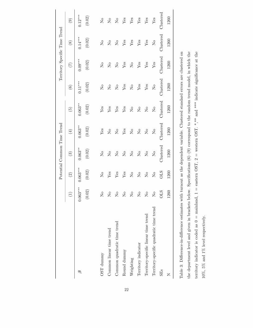
Table 3 displays the results of the baseline DID estimates and the random

trend model (in columns (6)-(9)). In the baseline DID regressions, the point esti-

mate is stable around 6.3 percentage points and significantly different from zero

across all specifications and the standard errors are almost unaffected by clus-

tering (columns (3) to (9)), implying that knowing the election results decreases

turnout by about 6 percentage points. In columns (6) and (7) we estimate the

basic random trend models and find that the point estimates increase somewhat

to 9 and 11 percentage points respectively. In columns (8) and (9) we estimate

the same territory-specific trend model using the size of the population in the

departments as weights. Doing so again results in slight increases in the treat-

ment coefficient to about 12 to 14 percentage points. Our preferred specification

is column (9) which includes territory specific linear and quadratic time trends,

a dummy indicating the election round and weighting. Here we estimate a treat-

22Hence turnout is also averaged over the two rounds by territory g, and year.

19

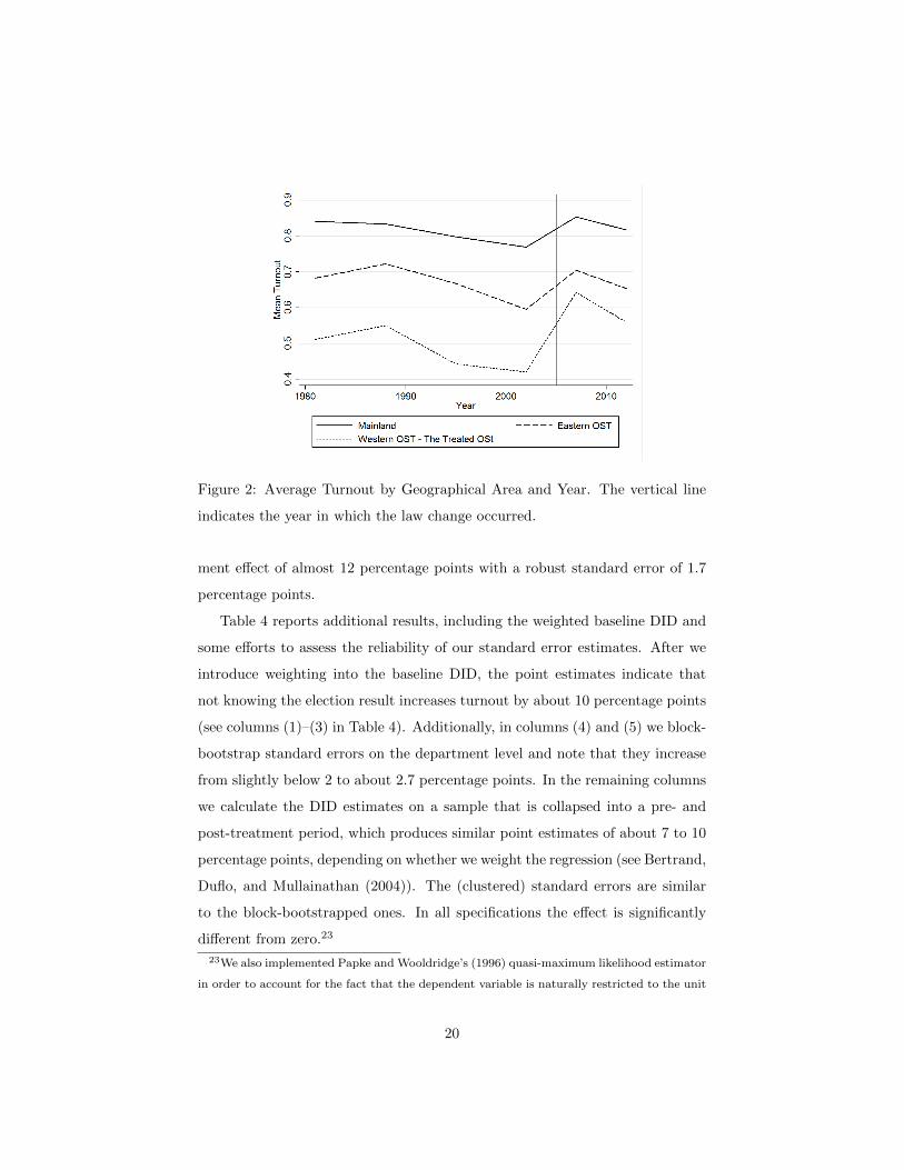
Figure 2: Average Turnout by Geographical Area and Year. The vertical line

indicates the year in which the law change occurred.

ment effect of almost 12 percentage points with a robust standard error of 1.7

percentage points.

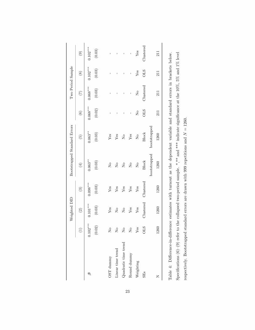
Table 4 reports additional results, including the weighted baseline DID and

some efforts to assess the reliability of our standard error estimates. After we

introduce weighting into the baseline DID, the point estimates indicate that

not knowing the election result increases turnout by about 10 percentage points

(see columns (1)–(3) in Table 4). Additionally, in columns (4) and (5) we block-

bootstrap standard errors on the department level and note that they increase

from slightly below 2 to about 2.7 percentage points. In the remaining columns

we calculate the DID estimates on a sample that is collapsed into a pre- and

post-treatment period, which produces similar point estimates of about 7 to 10

percentage points, depending on whether we weight the regression (see Bertrand,

Duflo, and Mullainathan (2004)). The (clustered) standard errors are similar

to the block-bootstrapped ones. In all specifications the effect is significantly

different from zero.23

23We also implemented Papke and Wooldridge’s (1996) quasi-maximum likelihood estimator

in order to account for the fact that the dependent variable is naturally restricted to the unit

20

In sum, in all specifications, the point estimate remains remarkably stable

and quite precisely estimated. For our preferred specification, we report an in-

crease in turnout from not knowing the election result of 12 percentage points.

Moreover, concerns about autocorrelation and different population sizes under-

lying each observation do not seem to matter.

interval. In this approach the conditional mean of the dependent variable is specified as a logit

function and the log likelihood as Bernoulli distributed. Since the Bernoulli likelihood is part

of the linear exponential function family, a quasi-maximum likelihood estimator is consistent

even when the Bernoulli distribution is misspecified. This result goes back to Gourieroux,

Monfort, and Trognon (1984). We cluster the standard errors in all cases on the department

level and find that the results are very much in line with earlier findings: not knowing the

election results has a significant positive impact on turnout.

21

Pote

nti

al

Com

mon

Tim

eT

ren

dT

erri

tory

Sp

ecifi

cT

ime

Tre

nd

(1)

(2)

(3)

(4)

(5)

(6)

(7)

(8)

(9)

β0.

063∗∗∗

0.0

63∗∗∗

0.063∗∗

0.0

63∗∗

0.063∗∗

0.1

1∗∗∗

0.09∗∗∗

0.14∗∗∗

0.1

2∗∗∗

(0.0

2)

(0.0

2)

(0.0

2)

(0.0

2)

(0.0

2)

(0.0

2)

(0.0

2)

(0.0

2)

(0.0

2)

OS

Td

um

my

No

No

No

Yes

Yes

No

No

No

No

Com

mon

lin

ear

tim

etr

end

No

Yes

No

No

Yes

No

No

No

No

Com

mon

qu

adra

tic

tim

etr

end

No

Yes

No

No

Yes

No

No

No

No

Rou

nd

du

mm

yN

oY

esN

oY

esY

esY

esY

esY

esY

es

Wei

ghti

ng

No

No

No

No

No

No

No

Yes

Yes

Ter

rito

ryin

dic

ator

No

No

No

No

No

Yes

Yes

Yes

Yes

Ter

rito

ry-s

pec

ific

lin

ear

tim

etr

end

No

No

No

No

No

Yes

Yes

Yes

Yes

Ter

rito

ry-s

pec

ific

qu

adra

tic

tim

etr

end

No

No

No

No

No

No

Yes

No

Yes

SE

sO

LS

OL

SC

lust

ered

Clu

ster

edC

lust

ered

Clu

ster

edC

lust

ered

Clu

ster

edC

lust

ered

N1260

1260

1260

1260

1260

1260

1260

1260

1260

Tab

le3:

Diff

eren

ce-i

n-d

iffer

ence

esti

mate

sw

ith

turn

ou

tas

the

dep

end

ent

vari

ab

le.

Clu

ster

edst

an

dard

erro

rsare

clu

ster

edon

the

dep

artm

ent

leve

lan

dgi

ven

inb

rack

ets

bel

ow.

Sp

ecifi

cati

on

s(6

)–(9

)co

rres

pon

dto

the

ran

dom

tren

dm

od

el,

inw

hic

hth

e

terr

itor

yin

dic

ator

isco

ded

as0

=m

ain

lan

d,

1=

east

ern

OS

T,

2=

wes

tern

OS

T.

*,*

*an

d***

ind

icate

sign

ifica

nce

at

the

10%

,5%

and

1%le

vel

resp

ecti

vely

.

22

Wei

ghte

dD

IDB

oots

trapp

edSta

ndard

Err

ors

Tw

oP

erio

dSam

ple

(1)

(2)

(3)

(4)

(5)

(6)

(7)

(8)

(9)

β0.1

02∗∗

∗0.1

01∗∗

∗0.0

98∗∗

∗0.0

63∗∗

0.0

63∗∗

0.0

68∗∗

∗0.0

68∗∗

∗0.1

02∗∗

∗0.1

02∗∗

∗

(0.0

2)

(0.0

3)

(0.0

3)

(0.0

3)

(0.0

3)

(0.0

2)

(0.0

3)

(0.0

3)

(0.0

3)

OST

dum

my

No

Yes

Yes

No

Yes

--

--

Lin

ear

tim

etr

end

No

No

Yes

No

Yes

--

--

Quadra

tic

tim

etr

end

No

No

Yes

No

No

--

--

Round

dum

my

No

Yes

Yes

No

Yes

--

--

Wei

ghti

ng

Yes

Yes

Yes

No

No

No

No

Yes

Yes

SE

sO

LS

Clu

ster

edC

lust

ered

Blo

ckB

lock

OL

SC

lust

ered

OL

SC

lust

ered

boots

trapp

edb

oots

trapp

ed

N1260

1260

1260

1260

1260

211

211

211

211

Tab

le4:

Diff

eren

ce-i

n-d

iffer

ence

esti

mate

sw

ith

turn

ou

tas

the

dep

end

ent

vari

ab

lean

dst

an

dard

erro

rsin

bra

cket

sb

elow

.

Sp

ecifi

cati

ons

(6)–

(9)

refe

rto

the

coll

ap

sed

two-p

erio

dsa

mp

le.

*,*

*an

d***

ind

icate

sign

ifica

nce

at

the

10%

,5%

an

d1%

leve

l

resp

ecti

vely

.B

oot

stra

pp

edst

and

ard

erro

rsare

dra

wn

wit

h999

rep

etit

ion

san

dN

=1260.

23

5 Robustness Checks

5.1 Pseudo-estimates and the Candidate from French Guiana

In order to check for robustness, we first calculate pseudo DID estimates us-

ing 1994 as the year in which reform was implemented (excluding post–2005

observations)24 and secondly (falsely) using the eastern OST as a treatment

group (on the full sample). In neither case do we find any significant coefficient

estimate (and hence the results are not reported here).

The first-time appearance in the first round of the 2002 election of a candi-

date from French Guiana might have led to an overly increased turnout in this

subdivision. As a consequence, our estimates might be biased since Guiana is

one of the treated territories. As the 2002 election is before the 2005 reform,

this bias would create a downward bias on the estimated effect of the reform on

the change in turnout. Given that we observe an increase in turnout following

the reform, the existence of a Guiana candidate in 2002 can only make our es-

timate conservative (meaning that the effect of exit poll information can only

be higher than the one estimated and not lower). In any case, we control for a

possible bias due to this event by including a dummy indicating Guiana in the

first round of 2002. As expected, we find a positive and significant coefficient on

this dummy. Nevertheless, all results from Table 3 remain literally unchanged

(and are thus not reported here), indicating that this event has no impact on

our estimates.

5.2 “Le Pen Elections”

In Section 3.3, we expressed concern that the anomalous result in the first

round of 2002 - in which right-wing candidate Jean-Marie Le Pen surprisingly

made it into the second round - might have impacted our results. First, we

24We prefer not to conduct this test on a sample that overlaps with 2005 since in this case

the treatment effect might potentially affect the pseudo-estimate. On the other hand, we only

observe four elections at two time points after the law changed. Hence it seems reasonable to

split the pre-treatment period into half and run this same test on that sample.

24

argue that this event is likely to downward bias our estimates, meaning that

we are presumably estimating lower bounds of the actual effect of knowing the

exit polls on turnout. Such is the case because the closeness of the election

is likely to increase turnout more in the west, which on average has better

information when voting, than in the eastern parts of France. As a result, the

DID estimates tend to be smaller than in the counterfactual case without this

highly polarizing candidate. Second, we replicate the regressions from Tables

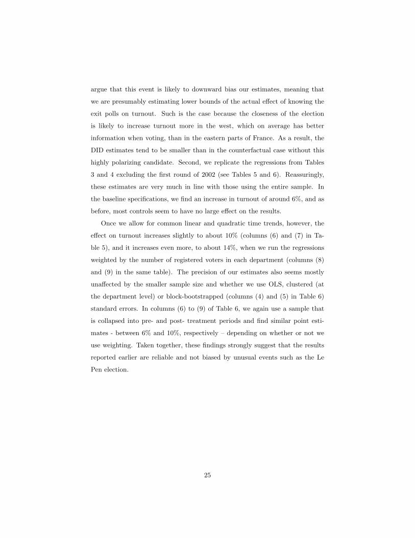
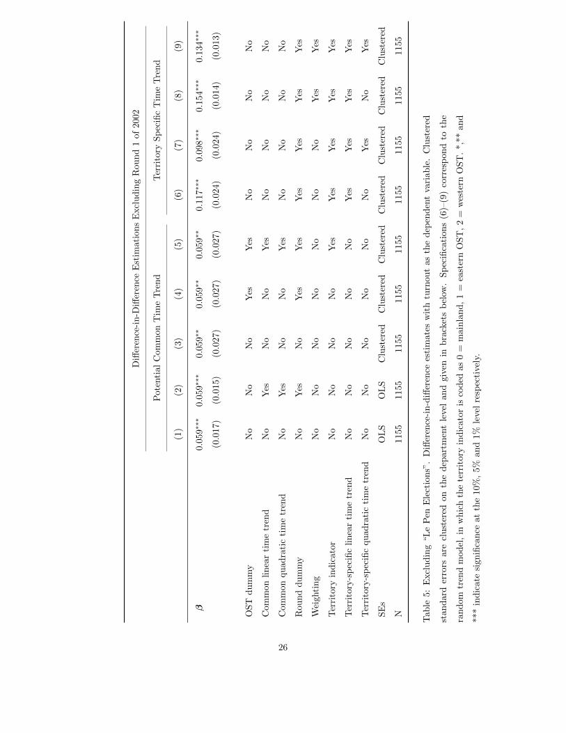
3 and 4 excluding the first round of 2002 (see Tables 5 and 6). Reassuringly,

these estimates are very much in line with those using the entire sample. In

the baseline specifications, we find an increase in turnout of around 6%, and as

before, most controls seem to have no large effect on the results.

Once we allow for common linear and quadratic time trends, however, the

effect on turnout increases slightly to about 10% (columns (6) and (7) in Ta-

ble 5), and it increases even more, to about 14%, when we run the regressions

weighted by the number of registered voters in each department (columns (8)

and (9) in the same table). The precision of our estimates also seems mostly

unaffected by the smaller sample size and whether we use OLS, clustered (at

the department level) or block-bootstrapped (columns (4) and (5) in Table 6)

standard errors. In columns (6) to (9) of Table 6, we again use a sample that

is collapsed into pre- and post- treatment periods and find similar point esti-

mates - between 6% and 10%, respectively – depending on whether or not we

use weighting. Taken together, these findings strongly suggest that the results

reported earlier are reliable and not biased by unusual events such as the Le

Pen election.

25

Diff

eren

ce-i

n-D

iffer

ence

Est

imati

ons

Excl

ud

ing

Rou

nd

1of

2002

Pote

nti

al

Com

mon

Tim

eT

ren

dT

erri

tory

Sp

ecifi

cT

ime

Tre

nd

(1)

(2)

(3)

(4)

(5)

(6)

(7)

(8)

(9)

β0.

059∗∗∗

0.0

59∗∗∗

0.059∗∗

0.0

59∗∗

0.059∗∗

0.117∗∗∗

0.098∗∗∗

0.1

54∗∗∗

0.134∗∗∗

(0.0

17)

(0.0

15)

(0.0

27)

(0.0

27)

(0.0

27)

(0.0

24)

(0.0

24)

(0.0

14)

(0.0

13)

OS

Td

um

my

No

No

No

Yes

Yes

No

No

No

No

Com

mon

lin

ear

tim

etr

end

No

Yes

No

No

Yes

No

No

No

No

Com

mon

qu

adra

tic

tim

etr

end

No

Yes

No

No

Yes

No

No

No

No

Rou

nd

du

mm

yN

oY

esN

oY

esY

esY

esY

esY

esY

es

Wei

ghti

ng

No

No

No

No

No

No

No

Yes

Yes

Ter

rito

ryin

dic

ator

No

No

No

No

Yes

Yes

Yes

Yes

Yes

Ter

rito

ry-s

pec

ific

lin

ear

tim

etr

end

No

No

No

No

No

Yes

Yes

Yes

Yes

Ter

rito

ry-s

pec

ific

qu

adra

tic

tim

etr

end

No

No

No

No

No

No

Yes

No

Yes

SE

sO

LS

OL

SC

lust

ered

Clu

ster

edC

lust

ered

Clu

ster

edC

lust

ered

Clu

ster

edC

lust

ered

N1155

1155

1155

1155

1155

1155

1155

1155

1155

Tab

le5:

Excl

ud

ing

“Le

Pen

Ele

ctio

ns”

.D

iffer

ence

-in

-diff

eren

cees

tim

ate

sw

ith

turn

ou

tas

the

dep

end

ent

vari

ab

le.

Clu

ster

ed

stan

dar

der

rors

are

clust

ered

onth

ed

epart

men

tle

vel

and

giv

enin

bra

cket

sb

elow

.S

pec

ifica

tion

s(6

)–(9

)co

rres

pon

dto

the

ran

dom

tren

dm

od

el,

inw

hic

hth

ete

rrit

ory

ind

icato

ris

cod

edas

0=

main

lan

d,

1=

east

ern

OS

T,

2=

wes

tern

OS

T.

*,*

*an

d

***

ind

icat

esi

gnifi

can

ceat

the

10%

,5%

an

d1%

leve

lre

spec

tive

ly.

26

Diff

eren

ce-i

n-D

iffer

ence

Est

imati

ons

Excl

udin

gR

ound

1of

2002

Wei

ghte

dD

IDB

oots

trapp

edSta

ndard

Err

ors

Tw

oP

erio

dSam

ple

(1)

(2)

(3)

(4)

(5)

(6)

(7)

(8)

(9)

β0.0

99∗∗

∗0.0

99∗∗

∗0.0

96∗∗

∗0.0

59∗∗

0.0

59∗∗

0.0

63∗∗

0.0

63∗∗

0.1

0∗∗

∗0.1

0∗∗

∗

(0.0

19)

(0.0

27)

(0.0

26)

(0.0

30)

(0.0

30)

(0.0

32)

(0.0

28)

(0.0

31)

(0.0

27)

OST

dum

my

No

Yes

Yes

No

Yes

--

--

Lin

ear

tim

etr

end

No

No

Yes

No

Yes

--

--

Quadra

tic

tim

etr

end

No

No

Yes

No

No

--

--

Round

dum

my

No

Yes

Yes

No

Yes

--

--

Wei

ghti

ng

Yes

Yes

Yes

No

No

No

No

Yes

Yes

SE

sO

LS

Clu

ster

edC

lust

ered

Blo

ckB

lock

OL

SC

lust

ered

OL

SC

lust

ered

boots

trapp

edb

oots

trapp

ed

N1155

1155

1155

1155

1155

211

211

211

211

Tab

le6:

Excl

ud

ing

“Le

Pen

Ele

ctio

ns”

.D

iffer

ence

-in

-Diff

eren

cees

tim

ate

sw

ith

turn

ou

tas

the

dep

end

ent

vari

ab

lean

dst

an

dard

erro

rsin

bra

cket

sb

elow

.S

pec

ifica

tion

s(6

)–(9

)re

fer

toth

eco

llap

sed

two-p

erio

dsa

mp

le.

*,*

*an

d***

ind

icate

sign

ifica

nce

at

the

10%

,5%

and

the

1%le

vel

resp

ecti

vely

.B

oots

trap

ped

stan

dard

erro

rsare

dra

wn

wit

h999

rep

etit

ion

san

dN

=1260.

27

5.3 Testing for Territory Specific Shocks on Turnout

A threat to the validity of our difference-in-difference estimates is differing time

paths for turnout in the territories versus the mainland in the absence of treat-

ment. We can credibly test for this concern by allowing for different linear and

quadratic time trends for the three territories (see Table 3). In our case, it is even

possible to go one step further by using turnout data on parliamentary elections

in France to re-estimate the same difference-in-difference models as in Section

3.5. Although these elections are national we would expect no treatment effect

because in each subdivision voters choose between different candidates who are

seeking the position as their local representative. Therefore, the result on the

mainland does not influence who will represent an OST district in the national

parliament.25 We can therefore test for territory-specific turnout shocks that

could potentially confound our estimates because such shocks, if they exist, are

likely to also affect other elections. While directly testing for these concerns is

essentially infeasible in DID models, our unique setting allows for this possibility.

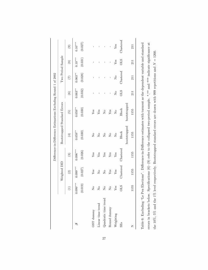
Table 7, which summarizes the results using the parliamentary data, shows

similar standard errors but much smaller coefficient estimates. Hence, given

that no estimated coefficients are significantly different from zero at the 10%

level and all are also much lower in absolute terms, OST-specific shocks do not

seem to be a concern. This finding assures us that we are indeed identifying the

causal effect of interest and not other time-variant shocks. As in Section 3.5, we

also introduce weighting but again find no significant point estimates. Figure 3

summarizes the turnout trends at these parliamentary elections by territory.

25It might be the case that voters in the OST care whether their local representative is a

member of a party of influence in the parliament and in that case results in the mainland may

affect their voting behavior. We assume that these concerns, if they exist, are not large.

28

No Common Time Trends Linear and Quadratic Time Trend

(1) (2) (3) (4) (5) (6)

β 0.02 0.02 0.02 0.02 0.02 0.01

(0.02) (0.03) (0.03) (0.02) (0.03) (0.03)

OST dummy No No Yes No Yes Yes

Round Dummy No No Yes Yes Yes Yes

Weighting No No No No No Yes

SEs OLS Clustered Clustered OLS Clustered Clustered

N 838 838 838 838 838 838

Table 7: Pseudo difference-in-difference estimates analogous to earlier tables

before with parliamentary election turnout as the dependent variable. Standard

errors are given in brackets below. The sample includes parliamentary elections

from 1997 to 2012. *,** and *** indicate significance at the 10%, 5% and 1%

level respectively.

29

Figure 3: Average turnout by territory and year for the parliamentary elec-

tions. The vertical line indicates the year in which the law changed. No over-

proportional increase in turnout is apparent in the western OST.

6 Estimating Potential Bandwagon Effects

In political science, the “bandwagon effect” refers to the phenomena where

people might vote for a candidate just because he or she is likely to win the

election.26 Although this effect attracted lots of attention among scholars, it

turned out to be quite difficult to provide empirical evidence. An opposite effect,

the “underdog” effect, where voters tend to favor the disadvantaged candidate,

26For a discussion of the psychological aspects of a bandwagon effect or impersonal influ-

ence, see, for example Kenney and Rice (1994) or Mutz (1997). Information can also affect

confidence in a voting decision (Matsusaka (1995)). An electoral momentum has also been

found in early presidential primaries (candidates performing well in Iowa or New Hampshire

receive a future primary voter boost, as discussed in Morton and Williams (1999) and Morton

and Williams (2001)). As reviewed previously, Callander (2007) provides a formal model of

bandwagon voting. See also the experimental evidence of bandwagon voting in Hung and

Plott (2001). Schmitt-Beck (1996) also refers to consensus heuristic. If a multitude of voters

are behind one of the candidates, people take the choice of others as an indicator of political

quality of the candidate.

30

has also been discussed as a possibility.27

The French natural experiment, however, provides a unique setting for ex-

amining such effects in that prior to the 2005 reform, voters in the western OST

knew the winner when they went to the polls. Our identification strategy thus

relies on estimating the impact of the leading presidential candidate’s voting

edge, as compared to that of the runner-up on the mainland (and in the eastern

OST), on the vote difference in the western OST. To determine this impact, we

estimate the following equation

∆s,t = α+ β∆mainland,t + γ1[t>2005] + δ∆mainland,t ∗ 1[t>2005] + εs,t, (2)

where ∆mainland,t ∈ [0, 1] is the normalized difference of votes between the can-

didate with the most votes and the runner–up at time t on the mainland (and

in the eastern OST) and ∆s,t ∈ [−1, 1] is the same difference in the western

departments at time t. We use only the vote difference in the western OST as

the left-hand variable in this estimation since the non-treated departments con-

tribute to ∆mainland,t. Our approach minimizes endogeneity concerns because

the regressors are predetermined. 1[.] once again denotes the indicator function.

Essentially, equation (2) estimates a pre- and post-2005 slope, in which the pa-

rameter of interest, δ, indicates the difference between both coefficients. This

approach allows us to test for a bandwagon effect using simple t-tests on δ. If

such an effect exists, we would expect δ to be significantly different from zero. A

negative δ would indicate that the results in west OSTs are less correlated with

mainland results after the reform (without exit poll information) than before

the reform (with exit poll information). Thus a negative parameter indicates a

bandwagon effect, where voters in western OST tended to follow the announced

mainland results before the reform. On the contrary, a positive δ indicates an

underdog effect with western OST voters voting less for the mainland favourite

27West (1991, p.153) discusses the case of Walter Mondale and Gary Hart in the 1984 US

presidential nominating process to illustrate the underdog effect. Mondale had a lead over

Hart. Hart then applied the strategy of “do not let the powerbrokers tell you the race is over.”

This strategy helped Hart to attract substantial amount of voter support, losing at the end

but performing much better than anticipated.

31

before the reform than after.

Our estimates are summarized in Table 8. We estimate equation (2) via

OLS and find a pre- treatment slope coefficient of 1.17, which is statistically

significant different from zero at the 1% level. We also find a large negative

slope coefficient of −4.05 for the post-2005 period. The difference δ between

both coefficients is therefore negative (−5.22) and statistically significant at the

10% level using ordinary clustered, and bootstrapped standard error estimates

(middle of Table 8) in the t-test. We also conduct a test of the equality of the

pre- and post-2005 slope coefficients (bottom of Table 8), which rejects equality

at the 1% level. Both coefficients, when taken alone, are statistically different

from zero, indicating that the positive relation when voters know who will win

turns negative after the law changes.

We also estimate the same equation excluding observations where the vote

edge from the mainland was larger than 20 percentage points (first round of

1988 and second round of 2002). Visual inspection of the raw data suggests

that these observations could be driving our estimates. Nevertheless, the last

column of Table 8 shows that such outlier observations are not a problem. The

point estimates and standard errors increase somewhat but all estimates are still

significant in all cases. Figure 4, which plots the fitted and raw ∆treated,st versus

∆mainland,t relation separately before and after 2005, confirms this conclusion

graphically.

Overall, these results clearly suggest that election results in western OSTs

were more positively correlated with the mainland results before the reform

when western OST voters could find out the winner in mainland results before

voting. In practice, the candidate ahead in mainland France was more likely to

win in western OSTs before the reform (when voters had access to information

on the identity of the leader on the mainland) than after the reform (when voters

no longer had access to such information). To our knowledge, the evidence we

have provided is the best from the field so far which demonstrates the existence

of a bandwagon effect.

32

Full Sample Excluding Outliers

Pre-2005 slope estimate 1.18∗∗∗ 7.45

(0.29) (4.71)

Post-2005 slope estimate −4.04∗ −4.04

(2.89) (3.07)

Difference δ −5.22 -11.49

Corresponding standard errors:

OLS (2.91)∗ (5.62)∗∗

Clustered by department (2.04)∗ (3.78)∗∗

Bootstrapped (1.23)∗∗∗ (5.76)∗∗

Block bootstrapped by department (1.73)∗∗∗ (3.31)∗∗∗

χ2 test of equality χ2 = 16.57∗∗∗ χ2 = 3.74∗

P value < 0.01 0.053

N 60 50

Table 8: Estimating equation (2) with ∆treated,st as the dependent variable.

Several standard error estimates are given for the t-test of H0 : the difference

in pre- and post-2005 slopes is zero. *,** and *** indicate significance for this

t-test at the 10%, 5% and 1% level, respectively.

33

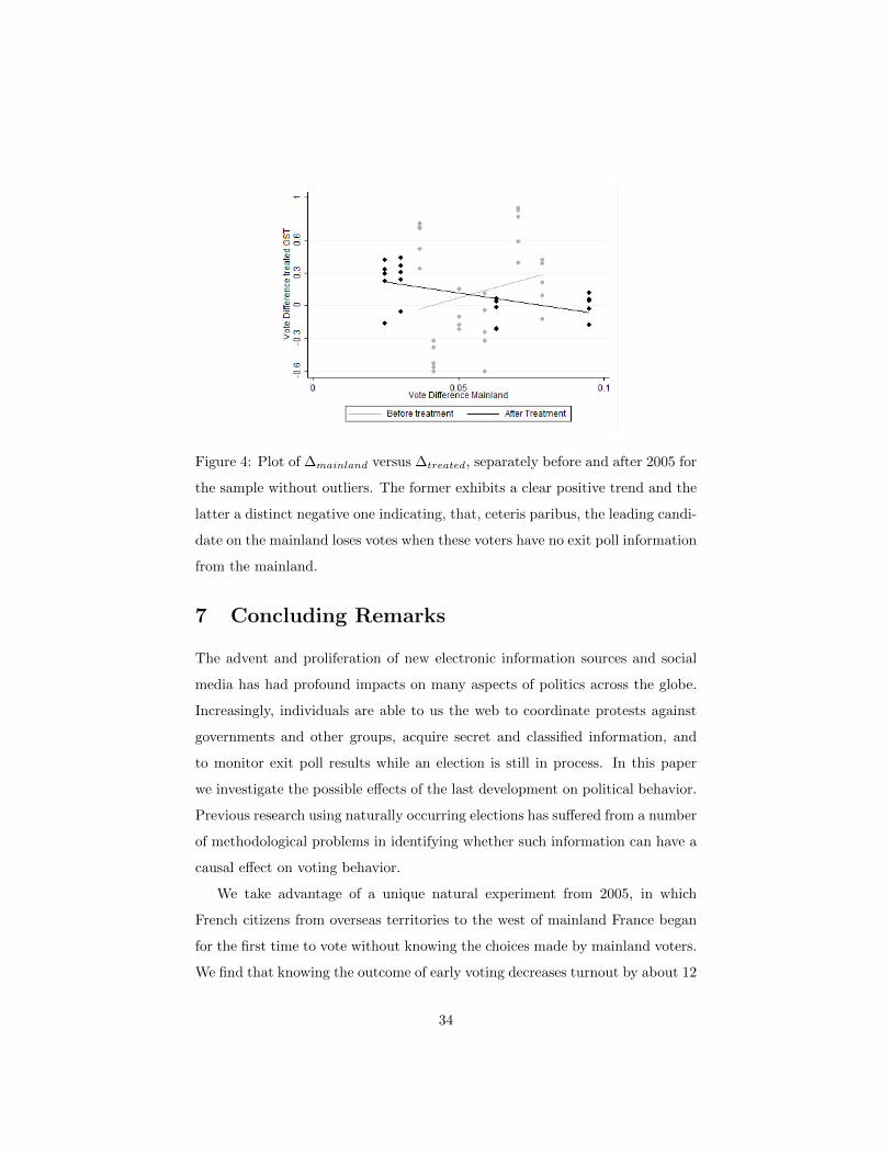
Figure 4: Plot of ∆mainland versus ∆treated, separately before and after 2005 for

the sample without outliers. The former exhibits a clear positive trend and the

latter a distinct negative one indicating, that, ceteris paribus, the leading candi-

date on the mainland loses votes when these voters have no exit poll information

from the mainland.

7 Concluding Remarks

The advent and proliferation of new electronic information sources and social

media has had profound impacts on many aspects of politics across the globe.

Increasingly, individuals are able to us the web to coordinate protests against

governments and other groups, acquire secret and classified information, and

to monitor exit poll results while an election is still in process. In this paper

we investigate the possible effects of the last development on political behavior.

Previous research using naturally occurring elections has suffered from a number

of methodological problems in identifying whether such information can have a

causal effect on voting behavior.

We take advantage of a unique natural experiment from 2005, in which

French citizens from overseas territories to the west of mainland France began

for the first time to vote without knowing the choices made by mainland voters.

We find that knowing the outcome of early voting decreases turnout by about 12

34

percentage points in our preferred specification. We also find empirical support

for bandwagon voting in which later voters, if they participate, are more likely

to vote for the expected winner.

Our results suggest that when voters can access exit poll results during

an election voting behavior is significantly affected. These effects on voting

behavior (lower participation and a bandwagon effect) provide advantages to

candidates and political parties favored by early voters, which do not exist in

the absence of the information. If later voters differ from early voters in terms

of demographics and ideological preferences, then we would also expect such

information to have an effect on the types of public policies chosen by elected

officials as well. Candidates and political parties, moreover, have an incentive

to manipulate the timing of voting and the type and accuracy of information

revealed through exit polls. Concerns about the effects of exit polls on elections

as expressed by many government officials, candidates, and party leaders and

calls for restrictions on such information are thus strongly supported by our

results.

References

Bale, T. (2002): “Restricting the broadcast and publication of pre-election

and exit polls: some selected examples,” Representation, 39(1), 15–22.

Battaglini, M. (2005): “Sequential voting with abstention,” Games and Eco-

nomic Behavior, 51(2), 445 – 463.

Battaglini, M., R. Morton, and T. Palfrey (2007): “Efficiency, eq-

uity, and timing of voting mechanisms,” American Political Science Review,

101(03), 409–424.

Bertrand, M., E. Duflo, and S. Mullainathan (2004): “How Much

Should We Trust Differences-In-Differences Estimates?,” Quarterly Journal

of Economics, 119(1), 249–275.

35

Best, S., and B. Krueger (2012): Exit Polls: Surveying the American Elec-

torate, 1927-2010. CQ Press.

Callander, S. (2007): “Bandwagons and momentum in sequential voting,”

Review of Economic Studies, 74(3), 653 – 684.

Carpini, M. (1984): “Scooping the voters? The consequences of the networks

early call of the 1980 presidential race,” Journal of Politics, 46(3), 866–885.

Carter, R. (2009): “German politicians livid at Twitter vote leak,” Agence

France Presse – English.

Dubois, P. (1983): “Election night projections and voter turnout in the west:

A Note on the Hazards of Aggregate Data Analysis,” American Politics Re-

search, 11(3), 349–364.

Gourieroux, C., A. Monfort, and A. Trognon (1984): “Pseudo Maxi-

mum Likelihood Methods: Theory,” Econometrica, 52(3), pp. 681 – 700.

Hung, A. A., and C. R. Plott (2001): “Information Cascades: Replication

and an Extension to Majority Rule and Conformity-Rewarding Institutions,”

American Economic Review, 91(5), pp. 1508 – 1520.

Jackson, J. (1983): “Election night reporting and voter turnout,” American

Journal of Political Science, 27(4), 615 – 635.

Kenney, P., and T. Rice (1994): “The psychology of political momentum,”

Political Research Quarterly, 47(4), 923–938.

Leonardo, S. (1983): “Restricting the Broadcast of Election-Day Projections:

A Justifiable Protection of the Right to Vote,” University of Dayton Law

Review, 9, 297.

Matsusaka, J. (1995): “Explaining voter turnout patterns: An information

theory,” Public Choice, 84(1), 91–117.

36

McAllister, I., and D. Studlar (1991): “Bandwagon, underdog, or projec-

tion? Opinion polls and electoral choice in Britain, 1979-1987,” Journal of

Politics, 53(3), 720–741.

Morton, R., and K. Williams (1999): “Information asymmetries and simul-

taneous versus sequential voting,” American Political Science Review, 93(1),

51–67.

Morton, R., and K. Williams (2001): Learning by voting: Sequential choices

in presidential primaries and other elections. University of Michigan Press.

Mutz, D. (1997): “Mechanisms of momentum: does thinking make it so?,”

Journal of Politics, 59(1), 104–125.

Papke, L., and J. Wooldridge (1996): “Econometric Methods for Fractional

Response Variables with an Application to 401 (K) Plan Participation Rates,”

Journal of Applied Econometrics, 11, 619–632.

Sayare, S. (2012): “French Media Question Election Reporting Rules,” New

York Times.

Schmitt-Beck, R. (1996): “Mass media, the electorate, and the bandwagon.

A study of communication effects on vote choice in Germany,” International

Journal of Public Opinion Research, 8(3), 266–291.

Spangenberg, F. (2003): “The freedom to publish opinion poll results: Report

on a worldwide update,” Amsterdam: Foundation for Information.

Sudman, S. (1986): “Do exit polls influence voting behavior?,” Public Opinion

Quarterly, 50(3), 331–339.

Thompson, D. (2004): “Election time: normative implications of temporal

properties of the electoral process in the United States,” American Political

Science Review, 98(01), 51–63.

Tuchman, S., and T. Coffin (1971): “The influence of election night televi-

sion broadcasts in a close election,” Public Opinion Quarterly, 35(3), 315–326.

37

West, D. (1991): “Polling effects in election campaigns,” Political Behavior,

13(2), 151–163.

Wooldridge, J. (2001): Econometric analysis of cross section and panel data.

MIT press.

38