Exact Inference on Multiple exponentialpopulations under A Joint Type-II

Progressive Censoring Scheme

Shuvashree Mondal∗, Debasis Kundu †

Abstract

Recently Mondal and Kundu [13] introduced a Type-II progressive censoring schemefor two populations. In this article we extend the above scheme for more than twopopulations. The aim of this paper is to study the statistical inference under the multisample Type-II progressive censoring scheme, when the underlying distributions areexponential. We derive the maximum likelihood estimators (MLEs) of the unknownparameters when they exist and find out their exact distributions. The stochasticmonotonicity of the MLEs has been established and this property can be used toconstruct exact confidence intervals of the parameters via pivoting the cumulativedistribution functions of the MLEs. The distributional properties of the ordered failuretimes are also obtained. The Bayesian analysis of the unknown model parameters hasbeen provided. We assume a very flexible gamma-Dirichlet prior and it turns outto be a conjugate prior also, when the sample sizes are equal. The performances ofthe different methods have been examined by extensive Monte Carlo simulations. Weanalyze two data sets for illustrative purpose. Finally we conclude the paper with someopen problems.

Key Words and Phrases: Type-II censoring scheme; progressive censoring scheme; joint

progressive censoring scheme; maximum likelihood estimator; confidence interval; bootstrap

confidence interval; simulation algorithm; conjugate prior.

AMS Subject Classifications: 62N01, 62N02, 62F10.

∗Department of Mathematics and Statistics, Indian Institute of Technology Kanpur, Pin 208016, India.†Department of Mathematics and Statistics, Indian Institute of Technology Kanpur, Pin 208016, India.

Corresponding author. E-mail: kundu@iitk.ac.in, Phone no. 91-512-2597141, Fax no. 91-512-2597500.

1

2

1 Introduction

In any life testing experiment censoring is inevitable, mainly to optimize cost and time. In the

literature an extensive amount of work has been done on different censoring schemes, specially

on single sample. Recently, Balakrishnan and Rasouli [5] introduced a Type-II censoring

scheme for two samples and provided the inference procedures of the unknown parameters

when the lifetime distributions are exponential. Ashour and Abo-Kasem [1] considered

Weibull populations under the joint Type-II censoring scheme proposed by Balakrishnan

and Rasouli [5]. Balakrishnan and Su [6] extended the results of Balakrishnan and Rasouli

[5] for multi sample cases.

Rasouli and Balakrishnan [20] introduced a joint Type-II progressive censoring scheme

and provided the likelihood and Bayesian inferences on two exponential populations under

the proposed scheme. From now onwards we call this scheme as a JPC-1 scheme. Parsi et al.

[17] studied likelihood inference under the JPC-1 scheme when the underlying distributions

are Weibull. Mondal and Kundu [14] provided order restricted inference of two Weibull

populations under the JPC-1 scheme. Balakrishnan et al. [7] extended the results of Rasouli

and Balakrishnan [20] for more than two populations.

Recently, Mondal and Kundu [13] introduced a new joint Type-II progressive censor-

ing scheme. It is observed that the scheme proposed by Mondal and Kundu [13] can be

implemented quite easily in practice and analytically it is more tractable than the scheme

proposed by Rasouli and Balakrishnan [20]. From now onwards the joint Type-II progressive

censoring scheme proposed by Mondal and Kundu [13] will be named as a JPC-2 scheme.

The JPC-2 scheme is a generalization of the self reallocated design (SRD), originally pro-

posed by Srivastava [21]. Mondal and Kundu [13] studied the inference on two exponential

distributions under the JPC-2 scheme. In this paper we extend the results of Mondal and

3

Kundu [13] for more than two populations.

The results under the two sample JPC-2 scheme are generalized for multi sample cases

when the underlying distributions are exponential. In this paper we derive maximum likeli-

hood estimators (MLEs) of the unknown parameters whenever they exist and provide their

exact distributions. Under the multi sample JPC-2 scheme, we obtain the distributional

properties of the censored order statistics and these results can be used for interval esti-

mation and for generating samples for the simulation experiment. Under the JPC-2 scheme

stochastic monotonicity of the MLEs can be established, hence exact confidence intervals can

be obtained via pivoting the cumulative distribution function (CDF) of the MLEs. Since,

exact confidence intervals are difficult to compute numerically, we propose to use bootstrap

confidence intervals of the parameters.

We further consider the Bayesian inference of the model parameters. We consider a

very flexible gamma-Dirichlet prior as a joint prior of the parameters. It turns out to be

a conjugate prior when the sample sizes are equal and in that case the Bayes estimators

based on the squared error loss function can be derived explicitly. Otherwise, we rely on the

importance sample technique to compute the Bayes estimates and the associated credible

intervals. We perform extensive simulation experiment to compare different methods and

the analyses of two data sets have been performed for illustrative purposes.

The main contribution of the present manuscript is two fold. First of all, we have extended

the classical inference of the two sample case of Mondal and Kundu [13] to multi sample

case. The main theoretical results of two sample case are based on Lemma 1 and Theorem 1

of Mondal and Kundu [13]. In the present manuscript those two results have been extended

in Lemma 3.2.1 and Theorem 3.2.1, respectively. Lemma 3.2.2 of the present manuscript is

purely a new result and that provides more insight about the behavior of the joint CDF of

the MLEs. But the major contribution of this present manuscript is the Bayesian inference

4

under a fairly general set of priors. Since, the construction of the exact confidence intervals

are quite complicated in practice, the Bayesian inference seems to be a natural choice, in

which finite sample inference can be obtained quite conveniently. The Bayesian inference was

not developed for the two sample case, and the present development can be easily applied

for the two sample case also.

Rest of the paper is organized as follows. In Section 2 we provide notations and briefly

discuss the JPC-2 scheme. In Section 3 the MLEs are derived along with their exact dis-

tributions and also we provide distributional properties of the censored order statistics. We

construct exact and bootstrap confidence interval in Section 4. In Section 5 we provide the

Bayes estimates and the associated credible intervals. In Section 6 simulation experiments

are performed along with real data analyses. Finally, we conclude the paper in Section 7.

2 Notation, Model Description and Model assump-

tion

2.1 Notation

CDF : Cumulative distribution function.

d= : equality in distribution.

HPD : Highest posterior density.

i.i.d : Independent and identically distributed.

MGF : Moment generated function.

MLE : Maximum likelihood estimator.

PDF: Probability density function.

∀h: Means for h = 1, . . . , H.

5

D(a1, a2, . . . , aH) : Multivariate Dirichlet distribution with PDF:

1

B(a1, a2, . . . , aH)

H∏h=1

xah−1h ; where xh > 0, ∀h,

H∑h=1

xh = 1,

B(a1, a2, . . . , aH) =

H∏h=1

Γ(ah)

Γ(a)and ah > 0, ∀h, a =

H∑h=1

ah.

Exp(θ) : Exponential distribution with PDF:

1

θe−

xθ ; x > 0, λ > 0.

GA(β, λ): Gamma distribution with PDF:

λβ

Γ(β)xβ−1e−λx; x > 0, λ, β > 0.

Mult(k, p1, p2, . . . , pH) : Multinomial distribution with probability mass function

P (K = r) = P (K1 = r1, K2 = r2, . . . , KH = rH) =k!

r1!r2! · · · rH !pr11 × pr22 × · · · × p

rHH ;

H∑h=1

rh = k, rh ∈ {1, 2, . . . , k} ,H∑h=1

ph = 1, ph ∈ [0, 1], ∀h.

Through out the paper it is assumed that the ‘small’ letter is the sample version of the

‘capital’ letter, and it should be clear from the context.

2.2 Model Description and Model assumption

Suppose we have H different populations. We draw independent samples of size nh from

the population h and call it as the sample h (Sam-h), ∀h. Let k ≤ min{n1, . . . , nH} be

the number of failures to be observed in the experiment and R1, . . . , Rk−1 are non-negative

integers satisfyingk−1∑i=1

(Ri + 1) < min{n1, . . . , nH}.

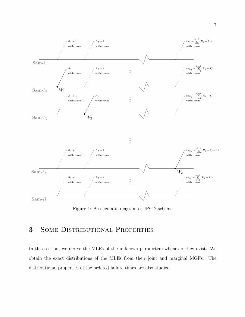
Under the JPC-2 scheme all the samples are put on a test simultaneously. Suppose

the first failure occurs at W1 from Sam-h1, then we remove R1 units randomly from the

6

remaining (nh1 − 1) units of Sam-h1 and we remove randomly R1 + 1 units each from the

remaining (H − 1) samples at W1. Next, suppose the second failure occurs from Sam-h2 at

W2. We remove R2 units from the remaining (nh2 − R1 − 2) surviving units of Sam-h2 and

R2 + 1 units each from the remaining surviving units from the rest of the (H − 1) samples.

We continue the experiment until the k-th failure occurs. At the k-th failure time point Wk,

we stop the experiment, see Mondal and Kundu [13] for details.

Under the JPC-2 scheme, along with W1, . . .Wk, we introduce another set of random

variables Zih, i = 1, . . . , k; ∀h, where Zih = 1, if i-th failure occurs from Sam-h and 0,

otherwise. Let Kh denote total number of failures coming from Sam-h. Under the JPC-2

scheme, the data set consists of (W,Z), where

W Z

W1 ( Z11, . . . , Z1H )...Wk ( Zk1,. . . , ZkH ).

HereH∑h=1

Zih = 1,k∑i=1

Zih = Kh andH∑h=1

k∑i=1

Zih =H∑h=1

Kh = k. In Figure 1 we provide a

schematic diagram of the JPC-2.

7

Sam-1

Sam-h1

Sam-h2

Sam-hk

Sam-H

R1 + 1

withdrawn

R1

withdrawn

W1

R1 + 1

withdrawn

R1 + 1

withdrawn

R1 + 1

withdrawn

R2 + 1

withdrawn

R2 + 1

withdrawn

R2

withdrawn

W2

R2 + 1

withdrawn

R2 + 1

withdrawn

(n1 −k−1∑j=1

(Rj + 1))

withdrawn

(nh1−

k−1∑j=1

(Rj + 1))

withdrawn

(nh2−

k−1∑j=1

(Rj + 1))

withdrawn

(nhk−

k−1∑j=1

(Rj + 1)− 1)

withdrawn

Wk

(nH −k−1∑j=1

(Rj + 1))

withdrawn

Figure 1: A schematic diagram of JPC-2 scheme

3 Some Distributional Properties

In this section, we derive the MLEs of the unknown parameters whenever they exist. We

obtain the exact distributions of the MLEs from their joint and marginal MGFs. The

distributional properties of the ordered failure times are also studied.

8

3.1 Maximum Likelihood Estimators

We assume that all the H populations are exponentially distributed. The sample from the

h-th population X1,h, X2,h, . . . , Xnh,h are i.i.d random variables from Exp(θh), ∀h.

For a given sampling scheme n1, n2, . . . , nH , k, R1, R2, . . . , Rk−1 and for the sample (w, z)

the likelihood function can be written as

L(θ1, . . . , θH |w, z) = C( H∏h=1

1

θkhh

)e−

H∑h=1

Ah(w)

θh , (1)

where

C =k∏i=1

( H∑h=1

(nh −i−1∑j=1

(Rj + 1))zih

),

Ah(w) =k−1∑i=1

(Ri + 1)wi + (nh −k−1∑i=1

(Ri + 1))wk, ∀h.

From (1), the MLE of θh is obtained as

θ̂h =Ah(w)

kh, ∀h.

It is clear that MLEs exist only when Kh > 0, ∀h. Hence (θ̂1, θ̂2, . . . , θ̂H) are conditional

MLEs conditioning on the eventM = {K = (K1, . . . , KH) :H∏h=1

Kh 6= 0} . We have used the

following usual convention that0∑i=1

ai = 0, for any arbitrary ai.

3.2 Exact Distribution of MLEs

We derive the exact distributions of MLEs from their joint and marginal MGFs. The fol-

lowing lemma is needed for further development.

Lemma 3.2.1 Let K = (K1, . . . , KH), r = (r1, . . . , rH) with rh ∈ {0, 1, . . . , k} andH∑h=1

rh =

k. Here Kh denotes the total number of failures from Sam-h, ∀h, as mentioned before.

9

Then,

P (K = r) =∑

z∈Q(r)

k∏i=1

( H∑h=1

(nh −i−1∑j=1

(Rj + 1))zih

)( H∏h=1

θrhh

)( k∏i=1

H∑h=1

(nh−i−1∑j=1

(Rj+1))

θh

) , (2)

where

Q(r) ={uk×H : u =

u11, . . . , u1H...

uk1, . . . , ukH

;uih ∈ {0, 1};

k∑i=1

uih = rh, ∀h;H∑h=1

uih = 1, for i = 1, . . . , k}.

Proof: See in the Appendix A.

Special Case: From (2) it is clear that when n1 = n2 = · · · = nH ,

P (K = r) =k!

r1!r2! · · · rH !pr11 × pr22 × · · · × p

rHH ,

where

ph =1θh

H∑l=1

1θl

.

Based on the conditioning on the event M, the joint MGF is given below.

Theorem 3.2.1 Let θ̂ = (θ̂1, . . . , θ̂H) and t = (t1, . . . , tH). Then the joint MGF of θ̂

conditioning on the event M, is obtained as

Mθ̂(t) =∑r∈S∗

P ∗r

k∏i=1

(1− αi,1

r1

t1 −αi,2r2

t2 − · · · −αi,HrH

tH

)−1

(3)

where

P ∗r =P (K = r)

P (M), αi,h =

(nh −i−1∑j=1

(Rj + 1))

H∑l=1

(nl−i−1∑j=1

(Rj+1))

θl

,

S∗ = {r = (r1, r2, . . . , rH) :H∏h=1

rh 6= 0,H∑h=1

rh = k}.

10

Proof: See in the Appendix A.

From the joint MGF, the joint CDF of θ̂ can be derived and we state the result in the

following lemma.

Lemma 3.2.2 The joint CDF of θ̂ can be obtained as

P (θ̂ ≤ x) =∑r∈S∗

P ∗r × P (G(r) ≤ x),

where G(r) is explicitly defined in Appendix A.

Proof: See in Appendix A.

Note that G(r) has a singular distribution function. Therefore, the joint PDF of θ̂ will

not exist. We derive the marginal MGFs and hence marginal PDFs.

Corollary 3.2.1 The marginal MGF of θ̂h, conditioning on the event M is given as

Mθ̂h(t) =

∑r∈S∗

P ∗r

k∏i=1

(1− αi,h

rht

)−1

. (4)

Special Case: When n1 = n2 = . . . = nH , αi,h = (H∑l=1

1θl

)−1 = α (say), ∀i = 1, . . . , k and

∀h. Therefore, the termk∏i=1

(1− αi,h

rht)−1

is turned out to be(1− α

rht)−k

.

Theorem 3.2.2 The marginal PDF of θ̂h, conditioning on the event M, is given as

fθ̂h(t) =∑r∈S∗

P ∗r × gYh,rh (t). (5)

If n1 = · · · = nH ,

gYh,rh (t) =rh

αkΓ(k)tk−1e−

rhαt; t > 0,

11

and otherwise

gYh,rh (t) =( k∏i=1

rhαi,h

)×

k∑i=1

e− rhαi,h

t∏kj=1,j 6=i

(rhαj,h− rh

αi,h

) ; t > 0.

Remark: gYh,rh (·) is the PDF of Yh,rh . When n1 = n2 = . . . = nH , Yh,rh follows GA(k, αrh

).

Therefore, for equal sample sizes, the distributions of the MLEs are the mixture of the gamma

distributions. Otherwise, all αi,h are distinct and Yh,rh =k∑i=1

U(i)h,rh

where U(i)h,rh∼ Exp(

αi,hrh

)

and they are independently distributed.

Then, P (θ̂h > t|M) is obtained as

P (θ̂h > t|M) =

∑r∈S∗

P ∗r ×∫∞t

rhαkΓ(k)

xk−1e−rhαxdx; t > 0 if n1 = . . . = nH

∑r∈S∗

P ∗r ×( k∏i=1

rhαi,h

)×

k∑i=1

(αi,hrh

)e− rhtαi,h∏k

j=1,j 6=i(rhαj,h− rhαi,h

); t > 0 otherwise.

Corollary 3.2.2 When n1 = n2 = . . . = nH ,

E(θ̂h) =∑r∈S∗

P ∗r ×kα

rh,

E(θ̂2h) =

∑r∈S∗

P ∗r ×k(k + 1)α2

r2h

.

E(θ̂h1 , θ̂h2) =∑r∈S∗

P ∗r ×k(k + 1)α2

rh1rh2.

Otherwise,

E(θ̂h) =∑r∈S∗

P ∗r ×( k∑i=1

αi,hrh

),

E(θ̂2h) =

∑r∈S∗

P ∗r ×(

2k∑i=1

(αi,hrh

)2

+k∑

i=1,i 6=j

αi,hαj,hrh2

).

E(θ̂h1 , θ̂h2) =∑r∈S∗

P ∗r ×(

2k∑i=1

(αi,h1αi,h2rh1rh2

) +k∑

i=1,i 6=j

αi,h1αj,h2rh1rh2

).

12

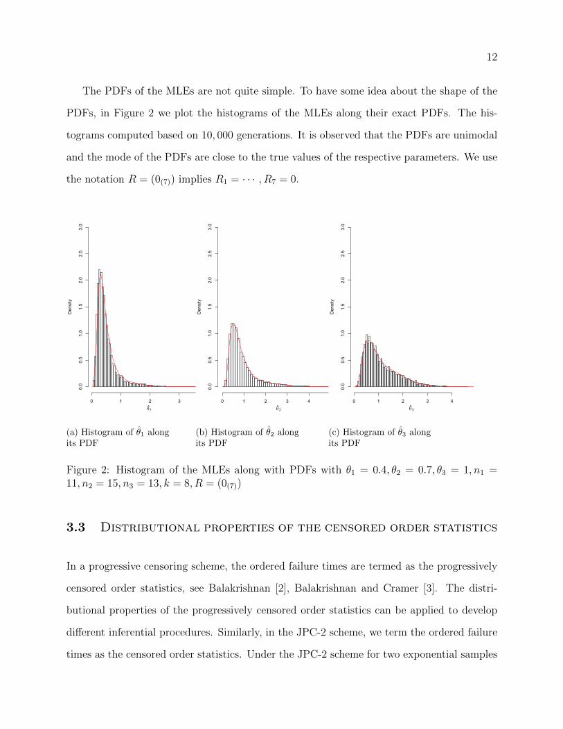
The PDFs of the MLEs are not quite simple. To have some idea about the shape of the

PDFs, in Figure 2 we plot the histograms of the MLEs along their exact PDFs. The his-

tograms computed based on 10, 000 generations. It is observed that the PDFs are unimodal

and the mode of the PDFs are close to the true values of the respective parameters. We use

the notation R = (0(7)) implies R1 = · · · , R7 = 0.

Den

sity

0 1 2 3 4

0.0

0.5

1.0

1.5

2.0

2.5

3.0

q̂1

(a) Histogram of θ̂1 alongits PDF

Den

sity

0 1 2 3 4 5

0.0

0.5

1.0

1.5

2.0

2.5

3.0

q̂2

(b) Histogram of θ̂2 alongits PDF

Den

sity

0 1 2 3 4

0.0

0.5

1.0

1.5

2.0

2.5

3.0

q̂3

(c) Histogram of θ̂3 alongits PDF

Figure 2: Histogram of the MLEs along with PDFs with θ1 = 0.4, θ2 = 0.7, θ3 = 1, n1 =11, n2 = 15, n3 = 13, k = 8, R = (0(7))

3.3 Distributional properties of the censored order statistics

In a progressive censoring scheme, the ordered failure times are termed as the progressively

censored order statistics, see Balakrishnan [2], Balakrishnan and Cramer [3]. The distri-

butional properties of the progressively censored order statistics can be applied to develop

different inferential procedures. Similarly, in the JPC-2 scheme, we term the ordered failure

times as the censored order statistics. Under the JPC-2 scheme for two exponential samples

13

we obtained the distributional properties of the censored order statistics, see in Mondal and

Kundu [13]. Here we extend those results for the general case.

Theorem 3.3.1 The censored order statistics W1 ≤ W2 ≤ . . . ≤ Wk have the following

distributional properties.

Wid=

i∑j=1

Vj

where Vj ∼ Exp( 1Ej

) and Ej =H∑h=1

(nh−j−1∑s=1

(Rs+1))

θh.

Proof: See in Appendix A.

This result can used for constructing confidence intervals and also to generate sample for

a JPC-2 scheme.

4 Construction of Confidence Intervals

4.1 Exact Confidence Intervals

The exact confidence interval of a real valued parameter θ can be obtained using the CDF

of a statistic T only if Pθ(T > t) is an increasing function of θ for any fixed t see for example

Casella and Berger [9], Lehmann and Romano [12]. Once this monotonicity assumption is

satisfied, a 100(1− γ)% confidence interval of θ can be obtained by solving Pθ(T > t) = γ1

and Pθ(T > t) = 1−γ2 where γ1+γ2 = γ. If the solutions exist, the monotonicity assumption

guarantees the uniqueness of the solutions of the above two equations.

In the JPC-2 scheme for exponential populations, the CDF of θ̂h can be obtained in

explicit form ∀h. As discussed above, the exact confidence interval can be obtained via

pivoting the CDF of θ̂h if the stochastic monotonicity property is satisfied. The following

lemma provides the necessary assumption of the monotonicity of Pθh(θ̂h > t), ∀h.

14

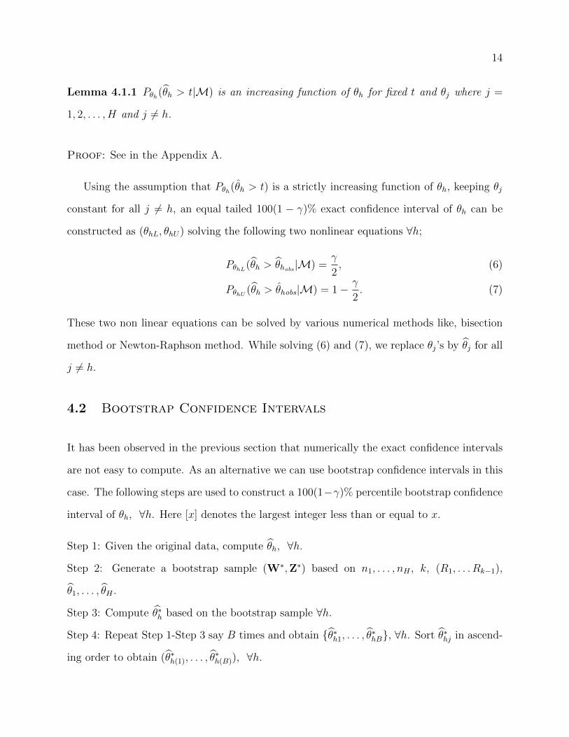
Lemma 4.1.1 Pθh(θ̂h > t|M) is an increasing function of θh for fixed t and θj where j =

1, 2, . . . , H and j 6= h.

Proof: See in the Appendix A.

Using the assumption that Pθh(θ̂h > t) is a strictly increasing function of θh, keeping θj

constant for all j 6= h, an equal tailed 100(1 − γ)% exact confidence interval of θh can be

constructed as (θhL, θhU) solving the following two nonlinear equations ∀h;

PθhL(θ̂h > θ̂hobs|M) =γ

2, (6)

PθhU (θ̂h > θ̂hobs|M) = 1− γ

2. (7)

These two non linear equations can be solved by various numerical methods like, bisection

method or Newton-Raphson method. While solving (6) and (7), we replace θj’s by θ̂j for all

j 6= h.

4.2 Bootstrap Confidence Intervals

It has been observed in the previous section that numerically the exact confidence intervals

are not easy to compute. As an alternative we can use bootstrap confidence intervals in this

case. The following steps are used to construct a 100(1−γ)% percentile bootstrap confidence

interval of θh, ∀h. Here [x] denotes the largest integer less than or equal to x.

Step 1: Given the original data, compute θ̂h, ∀h.

Step 2: Generate a bootstrap sample (W∗,Z∗) based on n1, . . . , nH , k, (R1, . . . Rk−1),

θ̂1, . . . , θ̂H .

Step 3: Compute θ̂∗h based on the bootstrap sample ∀h.

Step 4: Repeat Step 1-Step 3 say B times and obtain {θ̂∗h1, . . . , θ̂∗hB}, ∀h. Sort θ̂∗hj in ascend-

ing order to obtain (θ̂∗h(1), . . . , θ̂∗h(B)), ∀h.

15

Step 5: A 100(1 − γ)% bootstrap-p confidence interval of θh, ∀h, can be obtained as(θ̂∗h([ γ

2B]), θ̂

∗h([(1− γ

2)B])

).

5 Bayesian Analysis

In the previous section we have seen that exact confidence interval of the unknown parameters

cannot be obtained explicitly. Moreover, for any function of the parameters, it may not be

possible to construct the exact confidence interval. Hence, Bayesian analysis seems to be a

natural choice. Here we make the following re-parameterization λh = 1θh

, ∀h and we denote

λ = (λ1, λ2 . . . , λH).

5.1 Prior Assumption

Based on the idea of Pena and Gupta [18] it is assumed that( λ1

H∑h=1

λh

,λ2

H∑h=1

λh

, . . .λHH∑h=1

λh

)∼ D(a1, a2, . . . , aH),

H∑h=1

λh ∼ GA(a0, b0)

and they are independently distributed.

The joint PDF of λ is obtained as

π(λ|a0, b0, a1, a2, . . . , aH) ∝ (H∏h=1

λah−1h )(

H∑h=1

λh)

(a0−H∑h=1

ah)

e−b0

H∑h=1

λh, (8)

where the normalizing constant isba00

Γ(a0)B(a1,a2,...,aH).

We call this prior as the gamma-Dirichlet (GD(a0, b0, a1, a2, . . . , aH)) prior. When all the

sample sizes are equal, it is reduced to a conjugate prior. The hyper parameters namely a0,

b0, a1, a2,. . . , aH play important roles on the shape of the prior densities and on the mutual

dependence of λ′hs. WhenH∑h=1

ah = a0, λhs are mutually independent. Moreover, any two

16

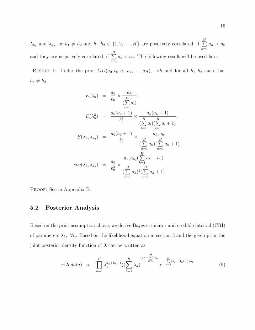
λh1 and λh2 for h1 6= h2 and h1, h2 ∈ {1, 2, . . . , H} are positively correlated, ifH∑h=1

ah > a0

and they are negatively correlated, ifH∑h=1

ah < a0. The following result will be used later.

Result 1: Under the prior GD(a0, b0, a1, a2, . . . , aH), ∀h and for all h1, h2 such that

h1 6= h2,

E(λh) =a0

b0

× ah

(H∑l=1

al)

,

E(λ2h) =

a0(a0 + 1)

b20

× ah(ah + 1)

(H∑l=1

al)(H∑l=1

al + 1)

,

E(λh1λh2) =a0(a0 + 1)

b20

× ah1ah2

(H∑h=1

ah)(H∑h=1

ah + 1)

.

cov(λh1λh2) =a0

b20

×ah1ah2(

H∑h=1

ah − a0)

(H∑h=1

ah)2(H∑h=1

ah + 1)

.

Proof: See in Appendix B.

5.2 Posterior Analysis

Based on the prior assumption above, we derive Bayes estimator and credible interval (CRI)

of parameters λh, ∀h. Based on the likelihood equation in section 3 and the given prior the

joint posterior density function of λ can be written as

π(λ|data) ∝ (H∏h=1

λah+kh−1h )(

H∑h=1

λh)

(a0−H∑h=1

ah)

e−

H∑h=1

(b0+Ah(w))λh(9)

17

5.2.1 Special case

When n1 = n2 = · · · = nH , all Ah(w) are equal and we denote A1(w) = · · · , AH(w) = B(w).

The joint posterior density of λ is obtained as

π(λ|data) ∼ GD(a0 + k, b0 +B(w), a1 + k1, a2 + k2, · · · , aH + kH).

Hence, in this case it turns out to be a conjugate prior. Therefore, the Bayes estimate of λh

based on the squared error loss function can be obtained as

λ̂hB = E(λh|data) =(a0 + k)

(b0 +B(w))× (ah + kh)

(H∑l=1

al + k)

.

The posterior variance and covariance are

V (λh|data) =(a0 + k)(ah + kh)

(b0 +B(w))2(H∑l=1

al + k)

×[(a0 + k + 1)(ah + kh + 1)

(H∑l=1

al + k + 1)

− (a0 + k)(ah + kh)

(H∑l=1

al + k)

]

and

cov(λh1 , λh2|data) =(a0 + k)

(b0 +B(w))2 ×(ah1 + kh1)(ah2 + kh2)(

H∑h=1

ah − a0)

(H∑h=1

ah + k)2(H∑h=1

ah + k + 1)

,

respectively. It is possible to provide a joint credible set of λ based on the following lemma.

Lemma 5.2.1 λ ∼ GD(a0 + k, b0 +B(w), a1 + k1, a2 + k2, . . . , aH + kH), if and only if

( λ1

H∑h=1

λh

,λ2

H∑h=1

λh

, . . .λHH∑h=1

λh

)∼ D(a1 + k1, a2 + k2, . . . , aH + kH),

H∑h=1

λh ∼ GA(a0 + k, b0 +B(w)) and they are independently distributed.

Proof: See in Appendix B.

18

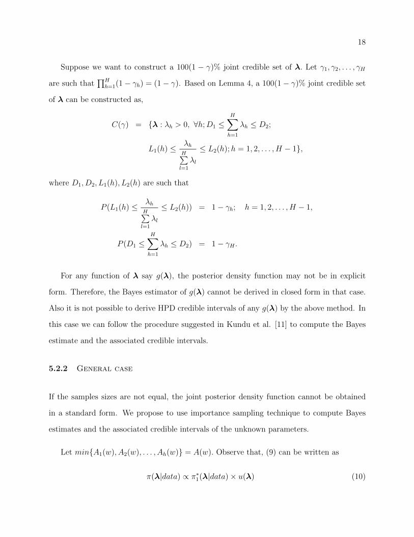
Suppose we want to construct a 100(1 − γ)% joint credible set of λ. Let γ1, γ2, . . . , γH

are such that∏H

h=1(1− γh) = (1− γ). Based on Lemma 4, a 100(1− γ)% joint credible set

of λ can be constructed as,

C(γ) = {λ : λh > 0, ∀h;D1 ≤H∑h=1

λh ≤ D2;

L1(h) ≤ λhH∑l=1

λl

≤ L2(h);h = 1, 2, . . . , H − 1},

where D1, D2, L1(h), L2(h) are such that

P (L1(h) ≤ λhH∑l=1

λl

≤ L2(h)) = 1− γh; h = 1, 2, . . . , H − 1,

P (D1 ≤H∑h=1

λh ≤ D2) = 1− γH .

For any function of λ say g(λ), the posterior density function may not be in explicit

form. Therefore, the Bayes estimator of g(λ) cannot be derived in closed form in that case.

Also it is not possible to derive HPD credible intervals of any g(λ) by the above method. In

this case we can follow the procedure suggested in Kundu et al. [11] to compute the Bayes

estimate and the associated credible intervals.

5.2.2 General case

If the samples sizes are not equal, the joint posterior density function cannot be obtained

in a standard form. We propose to use importance sampling technique to compute Bayes

estimates and the associated credible intervals of the unknown parameters.

Let min{A1(w), A2(w), . . . , Ah(w)} = A(w). Observe that, (9) can be written as

π(λ|data) ∝ π∗1(λ|data)× u(λ) (10)

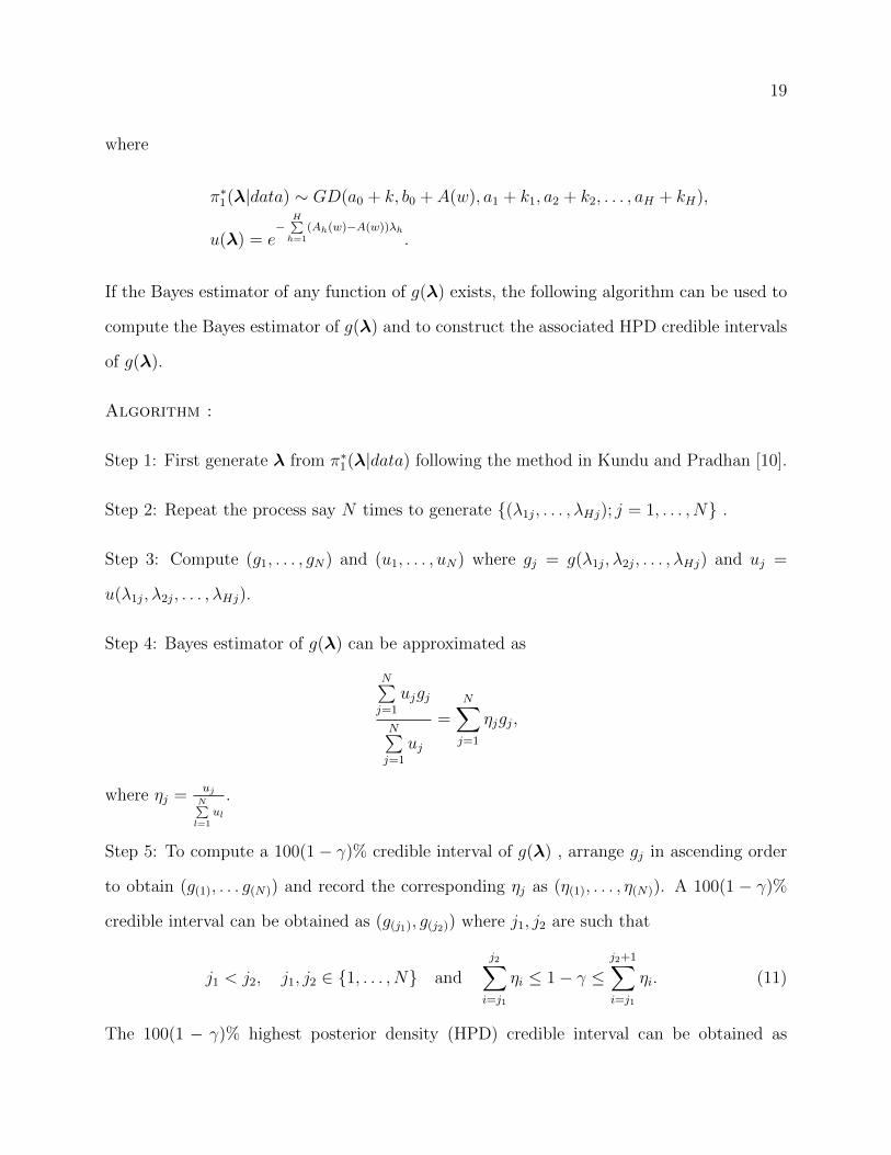
19

where

π∗1(λ|data) ∼ GD(a0 + k, b0 + A(w), a1 + k1, a2 + k2, . . . , aH + kH),

u(λ) = e−

H∑h=1

(Ah(w)−A(w))λh.

If the Bayes estimator of any function of g(λ) exists, the following algorithm can be used to

compute the Bayes estimator of g(λ) and to construct the associated HPD credible intervals

of g(λ).

Algorithm :

Step 1: First generate λ from π∗1(λ|data) following the method in Kundu and Pradhan [10].

Step 2: Repeat the process say N times to generate {(λ1j, . . . , λHj); j = 1, . . . , N} .

Step 3: Compute (g1, . . . , gN) and (u1, . . . , uN) where gj = g(λ1j, λ2j, . . . , λHj) and uj =

u(λ1j, λ2j, . . . , λHj).

Step 4: Bayes estimator of g(λ) can be approximated as

N∑j=1

ujgj

N∑j=1

uj

=N∑j=1

ηjgj,

where ηj =ujN∑l=1

ul

.

Step 5: To compute a 100(1− γ)% credible interval of g(λ) , arrange gj in ascending order

to obtain (g(1), . . . g(N)) and record the corresponding ηj as (η(1), . . . , η(N)). A 100(1 − γ)%

credible interval can be obtained as (g(j1), g(j2)) where j1, j2 are such that

j1 < j2, j1, j2 ∈ {1, . . . , N} and

j2∑i=j1

ηi ≤ 1− γ ≤j2+1∑i=j1

ηi. (11)

The 100(1 − γ)% highest posterior density (HPD) credible interval can be obtained as

20

(g(j∗1 ), g(j∗2 )), such that g(j∗2 )−g(j∗1 ) ≤ g(j2)−g(j1) and j∗1 , j∗2 satisfying (11) for all j1, j2 satisfying

(11).

6 Simulation study and Data Analysis

6.1 Simulation study

In this section we perform some simulation experiments to see how the proposed methods

work for different sample sizes and for different parameter values. We consider five exponen-

tial populations with mean θ1 = 0.3, θ2 = 0.4 θ3 = 0.5, θ4 = 0.6 and θ5 = .7. Different sample

sizes (n1, n2, n3, n4, n5), different effective sample size k and different choices of R1, . . . , Rk−1

are considered. We use the following notation to denote a particular JPC-2 censoring scheme,

for fixed k = 10 and R = (5, 0(18)) indicates R1 = 5 and R2 = · · · = R19 = 0.

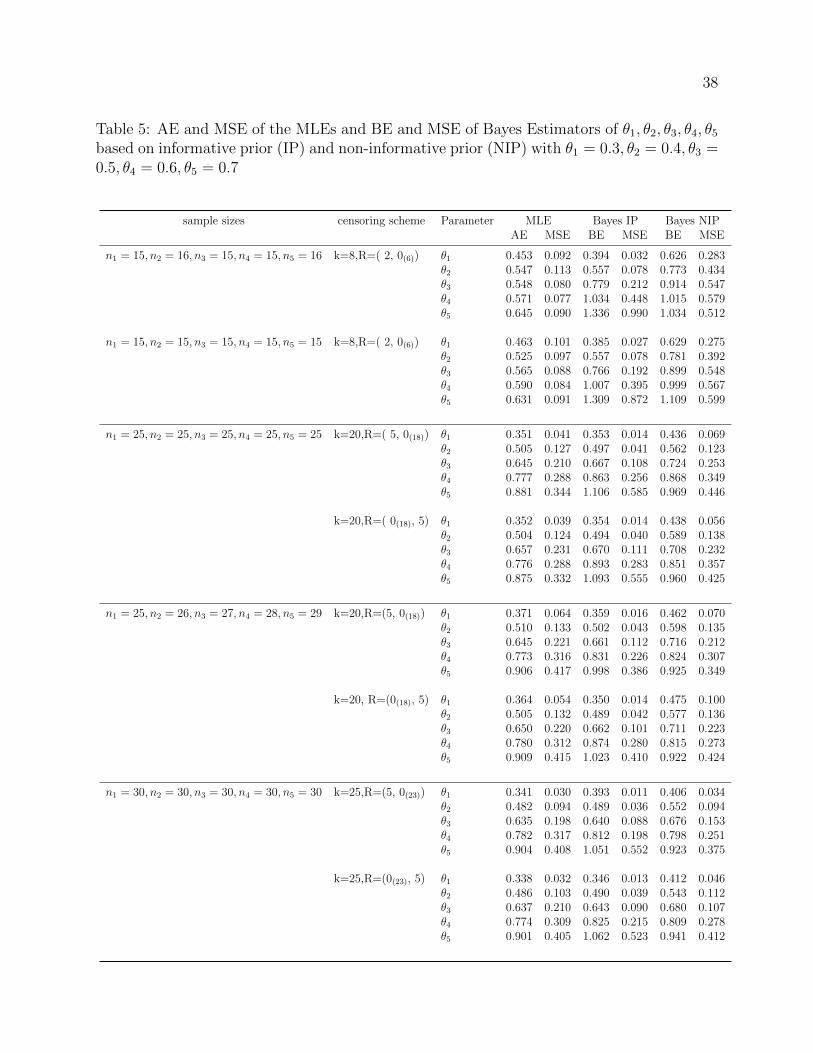
In each case, we compute the MLEs of the parameters. In Table 5 we record the average

estimates (AEs) and the corresponding mean squared errors (MSEs) of the MLEs based on

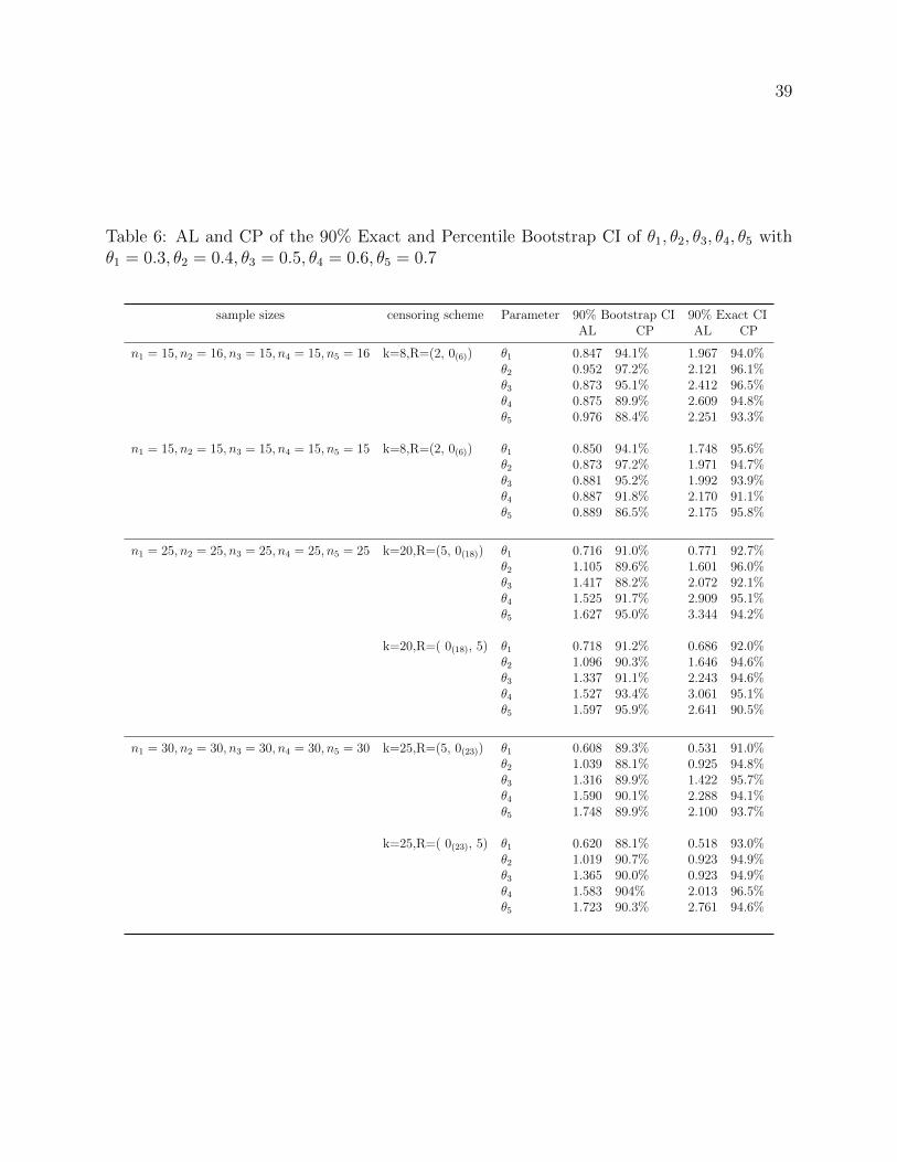
10, 000 replications. We also construct 90% exact and bootstrap confidence intervals. In

Table 6 we report the average length (AL) and the corresponding coverage percentage (CP)

of those intervals based on 1000 replications. For bootstrap interval estimation, for each

replication we have used 1000 re-samplings.

In Bayesian analysis we compute the Bayes estimates based on the squared error loss

function and the associated HPD and symmetric credible intervals both for informative and

non-informative priors. For informative prior we set a0 = 1, b0 = 0.091, a1 = 5, a2 = 3.7, a3 =

3, a4 = 2.5, a5 = 2.142. These values are chosen by equating the prior expectations with the

true values of the parameters so that prior variance of θhs exist for h = 1, 2, 3, 4, 5. In case

of non-informative priors, we have assumed that a0 = b0 = 0 and a1 = a2 = a3 = a4 = a5 =

2.005. Note that we have chosen ah > 2 for h = 1, 2, 3, 4, 5, as it ensures the existence of the

21

posterior variance of θh for h = 1, 2, 3, 4, 5.

In Table 5 we compute the average Bayes estimates (BE) and corresponding MSEs based

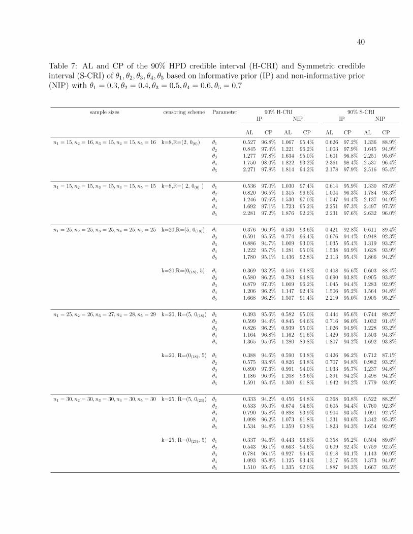
on 1000 samples both for informative and non-informative priors. We record the AL and

the CP of the 90% HPD and symmetric credible intervals both for informative and non-

informative priors in Table 7. These figures are computed based on 1000 replications.

It is observed that both MLEs and Bayes estimates are biased estimates, and the biases

are positive. Though for the small effective sample size k, the MLEs perform better in terms

of the average bias and the MSE than the non-informative prior based Bayes estimators, for

moderate to large values of k, they perform more or less similar. Another important point

is that, though for θ1, θ2, θ3, θ4, the informative prior based Bayes estimators perform better

than the non-informative prior based Bayes estimators and the MLEs in terms of the average

bias and the MSEs, but for θ5 which is the largest among five parameters, the performance of

informative prior based Bayes estimators is sometimes worse than the other two estimators.

In interval estimation the bootstrap intervals are performing better than the exact confi-

dence intervals in terms of the average lengths. For exact intervals the CPs always exceed the

nominal levels. But to find out the exact confidence intervals, we need to solve two non-linear

equations (6) and (7). Depending upon the choice of sample sizes, effective sample size, the

censoring scheme and the maximum likelihood estimates, the solution of these two equations

may not exist. Again for moderate to large values of sample sizes, when all the sample sizes

are not equal, solving these two equations becomes computationally challenging. But the

bootstrap confidence intervals have no such issues and can be derived conveniently.

Both for informative and non-informative priors, HPD credible intervals provide shorter

lengths than the corresponding symmetric CRIs. All the cases CPs are very close to the nom-

inal level. From these extensive simulation experiments, the effect of the hyper parameters

22

are also quite clear. It is observed that in case of the informative priors the biases, MSEs

and the length of the credible intervals are also smaller compared to the non-informative

priors.

6.2 Data Analysis

In this section we present the analyses of two real data sets for illustrative purposes.

Example 1. Nelson [15] ( Chapter-1, Table 1.1) provided the data, containing the times

to breakdown of an insulating fluid between electrodes recorded at seven different voltages.

For illustrative purposes we choose the breakdown times at voltage 32 KV, 34 KV, 36 KV

and 38 KV. The data are presented below for easy reference.

Data set 1 (Breakdown at 32 KV): 0.27, 0.40, 0.69, 0.79, 2.75, 3.91, 9.88, 13.95, 15.93, 27.80,

53.24, 82.85, 89.29, 100.58, 215.10.

Data set 2 (Breakdown at 34 KV): 0.19, 0.78,0.96, 1.31, 2.78, 3.16, 4.15, 4.67, 4.85, 6.50,

7.35, 8.01, 8.27, 12.06, 31.75, 32.52,33.91, 36.71, 72.89.

Data set 3 (Breakdown at 36 KV): 0.35, 0.59 , 0.96, 0.99, 1.69, 1.97, 2.07, 2.58, 2.71,2.90,

3.67, 3.99, 5.35, 13.77, 25.50.

Data set 4 (Breakdown at 38 KV): 0.09, 0.39, 0.47, 0.73, 0.74, 1.13, 1.40, 2.38.

Here H = 4 and n1 = 15, n2 = 19, n3 = 15, n4 = 8. It is observed that the exponential

distribution fits the data sets quite well.

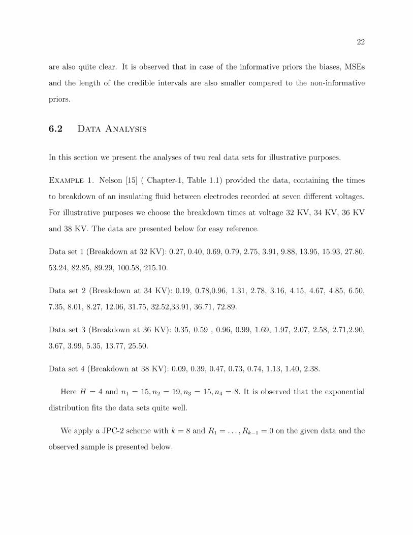
We apply a JPC-2 scheme with k = 8 and R1 = . . . , Rk−1 = 0 on the given data and the

observed sample is presented below.

23

Table 1: JPC-2 sample (example 1)

W Z

0.09 ( 0, 0,0,1 )0.19 ( 0, 1,0,0 )0.27 ( 1, 0,0,0 )0.35 ( 0, 0,1,0)0.40 ( 1, 0,0,0 )0.47 ( 0, 0,0,1 )0.69 ( 1, 0,0,0 )0.74 ( 0, 0,0,1 )

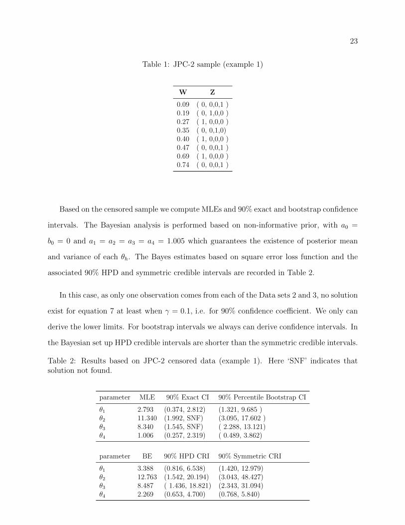
Based on the censored sample we compute MLEs and 90% exact and bootstrap confidence

intervals. The Bayesian analysis is performed based on non-informative prior, with a0 =

b0 = 0 and a1 = a2 = a3 = a4 = 1.005 which guarantees the existence of posterior mean

and variance of each θh. The Bayes estimates based on square error loss function and the

associated 90% HPD and symmetric credible intervals are recorded in Table 2.

In this case, as only one observation comes from each of the Data sets 2 and 3, no solution

exist for equation 7 at least when γ = 0.1, i.e. for 90% confidence coefficient. We only can

derive the lower limits. For bootstrap intervals we always can derive confidence intervals. In

the Bayesian set up HPD credible intervals are shorter than the symmetric credible intervals.

Table 2: Results based on JPC-2 censored data (example 1). Here ‘SNF’ indicates thatsolution not found.

parameter MLE 90% Exact CI 90% Percentile Bootstrap CI

θ1 2.793 (0.374, 2.812) (1.321, 9.685 )θ2 11.340 (1.992, SNF) (3.095, 17.602 )θ3 8.340 (1.545, SNF) ( 2.288, 13.121)θ4 1.006 (0.257, 2.319) ( 0.489, 3.862)

parameter BE 90% HPD CRI 90% Symmetric CRI

θ1 3.388 (0.816, 6.538) (1.420, 12.979)θ2 12.763 (1.542, 20.194) (3.043, 48.427)θ3 8.487 ( 1.436, 18.821) (2.343, 31.094)θ4 2.269 (0.653, 4.700) (0.768, 5.840)

24

Example 2:

Nelson [15] (Chapter 10 , Table 4.1) presented times to breakdown in minutes of an

insulating fluid subjected to high voltage stress. The breakdown times were presented in six

groups and each group is of size 10. For our analysis purpose we choose group 1, 2 and 3

and exponential distribution fits the data sets quite well.

Group 1: 0.31, 0.66, 1.54, 1.70, 1.82, 1.89, 2.17, 2.24, 4.03, 9.99.

Group 2: 0.00, 0.18, 0.55, 0.66, 0.71, 1.30, 1.63, 2.17, 2.75, 10.60.

Group 3: 0.49, 0.64 ,0.82 ,0.93 ,1.08, 1.99, 2.06, 2.15, 2.57, 4.75.

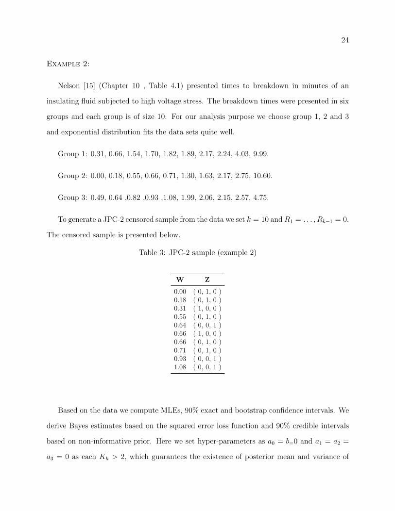
To generate a JPC-2 censored sample from the data we set k = 10 andR1 = . . . , Rk−1 = 0.

The censored sample is presented below.

Table 3: JPC-2 sample (example 2)

W Z

0.00 ( 0, 1, 0 )0.18 ( 0, 1, 0 )0.31 ( 1, 0, 0 )0.55 ( 0, 1, 0 )0.64 ( 0, 0, 1 )0.66 ( 1, 0, 0 )0.66 ( 0, 1, 0 )0.71 ( 0, 1, 0 )0.93 ( 0, 0, 1 )1.08 ( 0, 0, 1 )

Based on the data we compute MLEs, 90% exact and bootstrap confidence intervals. We

derive Bayes estimates based on the squared error loss function and 90% credible intervals

based on non-informative prior. Here we set hyper-parameters as a0 = b=0 and a1 = a2 =

a3 = 0 as each Kh > 2, which guarantees the existence of posterior mean and variance of

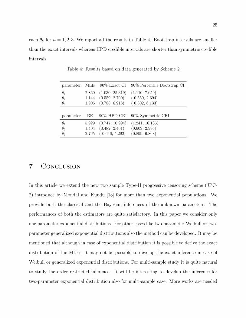
25

each θh for h = 1, 2, 3. We report all the results in Table 4. Bootstrap intervals are smaller

than the exact intervals whereas HPD credible intervals are shorter than symmetric credible

intervals.

Table 4: Results based on data generated by Scheme 2

parameter MLE 90% Exact CI 90% Percentile Bootstrap CI

θ1 2.860 (1.030, 25.319) (1.110, 7.659)θ2 1.144 (0.559, 2.700) ( 0.550, 2.694)θ3 1.906 (0.788, 6.918) ( 0.802, 6.133)

parameter BE 90% HPD CRI 90% Symmetric CRI

θ1 5.929 (0.747, 10.994) (1.241, 16.136)θ2 1.404 (0.482, 2.461) (0.609, 2.995)θ3 2.765 ( 0.646, 5.292) (0.899, 6.868)

7 Conclusion

In this article we extend the new two sample Type-II progressive censoring scheme (JPC-

2) introduce by Mondal and Kundu [13] for more than two exponential populations. We

provide both the classical and the Bayesian inferences of the unknown parameters. The

performances of both the estimators are quite satisfactory. In this paper we consider only

one parameter exponential distributions. For other cases like two-parameter Weibull or two-

parameter generalized exponential distributions also the method can be developed. It may be

mentioned that although in case of exponential distribution it is possible to derive the exact

distribution of the MLEs, it may not be possible to develop the exact inference in case of

Weibull or generalized exponential distributions. For multi-sample study it is quite natural

to study the order restricted inference. It will be interesting to develop the inference for

two-parameter exponential distribution also for multi-sample case. More works are needed

26

in those directions.

Acknowledgements:

The authors would like to thank two unknown reviewers and also the associate editor for

many constructive suggestions which have helped to improve the paper significantly. Part

of the work of the second author has been supported by a grant from the Department of

Science and Technology, Government of India, No. MTR/2018/000179.

Appendix A

Proof of lemma 3.2.1:

If d1, . . . , dk > 0, then

∞∫0

∞∫w1

. . .

∞∫wk−1

e−

k∑i=1

diwidwk . . . dw2dw1 =

1

dk(dk + dk−1) · · · (dk + dk−1 + · · ·+ d1). (12)

P (K = r) =∑

z∈Q(r)

∞∫0

∞∫w1

. . .

∞∫wk−1

L(θ1, θ2, . . . , θH |w, z)dwk . . . dw2dw1

=∑

z∈Q(r)

C( H∏h=1

1

θrhh

) ∞∫0

∞∫w1

. . .

∞∫wk−1

e−

H∑h=1

Ah(w)

θh dwk . . . dw2dw1

=∑

z∈Q(r)

C( H∏h=1

1

θrhh

) ∞∫0

∞∫w1

. . .

∞∫wk−1

e−

k∑i=1

aiwidwk . . . dw2dw1,

where ai =H∑h=1

(Ri+1)θh

for i = 1, . . . , k − 1 and ak =H∑h=1

(nh−k−1∑i=1

(Ri+1))

θh.

27

Using(12)

P (K = r) =∑

z∈Q(r)

C( H∏h=1

1

θrhh

) 1

ak(ak + ak−1) · · · (ak + ak−1 + · · ·+ a1)

=∑

z∈Q(r)

C( H∏h=1

1

θrhh

) 1(∏ki=1

H∑h=1

(nh−i−1∑j=1

(Rj+1))

θh

) .

Substituting C =∏k

i=1

( H∑h=1

(nh −i−1∑j=1

(Rj + 1))zih

),

P (K = r) =∑

z∈Q(r)

∏ki=1

( H∑h=1

(nh −i−1∑j=1

(Rj + 1))zih

)(∏H

h=1 θrhh

)(∏ki=1

H∑h=1

(nh−i−1∑j=1

(Rj+1))

θh

) .

Proof of Theorem 3.2.1:

Mθ̂(t)) = E(etθ̂|M

)=

∑r∈S∗

E(etθ̂|K = r)P (K = r|M)

=∑

z∈Q(r)

∑r∈S∗

E(etθ̂|Z = z,K = r)P (Z = z|K = r)P (K = r|M)

=1

P (M)

∑z∈Q(r)

∑r∈S∗

C( H∏h=1

1

θrhh

) ∞∫0

∞∫w1

. . .

∞∫wk−1

e−

k∑i=1

biwidwk . . . dw2dw1

where

bi =H∑h=1

(Ri + 1)

θh− t1

(Ri + 1)

r1

− t2(Ri + 1)

r2

− · · · − tH(Ri + 1)

rH∀ i = 1, . . . , k − 1,

bk =H∑h=1

(nh −k−1∑i=1

(Ri + 1))

θh− t1

(n1 −k−1∑i=1

(Ri + 1))

r1

− t2(n2 −

k−1∑i=1

(Ri + 1))

r2

− · · · − tH(nH −

k−1∑i=1

(Ri + 1))

rH.

28

Using(12) we obtain

Mθ̂(t)) =1

P (M)

∑z∈Q(r)

∑r∈S∗

C( H∏h=1

1

θrhh

) 1

bk(bk + bk−1) · · · (bk + bk−1 + · · ·+ b1)

=1

P (M)

∑z∈Q(r)

∑r∈S∗

C( H∏h=1

1

θrhh

)×

1

∏ki=1

( H∑h=1

(nh−i−1∑j=1

(Rj+1))

θh− t1

(n1−i−1∑j=1

(Rj+1))

r1· · · − tH

(nH−i−1∑j=1

(Rj+1))

rH

)=

1

P (M)

∑z∈Q(r)

∑r∈S∗

C( H∏h=1

1

θrhh

) 1

∏ki=1

( H∑h=1

(nh−i−1∑j=1

(Rj+1))

θh

) ×1

∏ki=1

(1− t1

(n1−i−1∑j=1

(Rj+1))

r1

(H∑h=1

(nh−i−1∑j=1

(Rj+1))

θh

) − · · · − tH (nH−i−1∑j=1

(Rj+1))

rH

(H∑h=1

(nh−i−1∑j=1

(Rj+1))

θh

))

Substituting C =∏k

i=1

( H∑h=1

(nh −i−1∑j=1

(Rj + 1))zih

),

Mθ̂(t))) =1

P (M)

∑z∈Q(r)

∑r∈S∗

k∏i=1

( H∑h=1

(nh −i−1∑j=1

(Rj + 1))zih

)×

( H∏h=1

1

θrhh

) 1

∏ki=1

( H∑h=1

(nh−i−1∑j=1

(Rj+1))

θh

) ×1

∏ki=1

(1− t1

(n1−i−1∑j=1

(Rj+1))

r1

(H∑h=1

(nh−i−1∑j=1

(Rj+1))

θh

) − · · · − tH (nH−i−1∑j=1

(Rj+1))

rH

(H∑h=1

(nh−i−1∑j=1

(Rj+1))

θh

))

=1

P (M)

∑r∈S∗

P (K = r)k∏i=1

(1− t1

αi,1r1

− · · · − tHαi,HrH

)−1

.

Proof of Lemma 3.2.2:

29

Let V= (a1U, . . . , aHU) where U ∼ Exp(1) and t =(t1, . . . , tH), x = (x1, . . . , xH). Then

the MGF of V is obtained as

MV(t) = (1− a1t1 − . . .− aHtH)−1

and the CDF is

FV(x) = 1− e− min

1≤h≤H(xhah

).

Clearly, V follows a singular distribution and we denote it by F (a1, . . . , aH).

Let Vi(r) ∼ F (αi,1r1, · · · , αi,H

rH) independently for i = 1, . . . , k and ∀ r = (r1, . . . , rH) ∈ S∗.

We define

G(r) =k∑i=1

Vi(r). (13)

Then the MGF of G(r) is

k∏i=1

(1− αi,1

r1

t1 −αi,2r2

t2 − · · · −αi,HrH

tH)−1

Therefore, the result follows.

The joint CDF of G(r) can be obtained as

P (G(r) < x)

= P( k∑i=1

Vi(r) ≤ x)

= P( k∑i=1

αi,1r1

Ui ≤ x1, . . . ,k∑i=1

αi,HrH

Ui ≤ xH

)

=

minh

(xhαk,hrh

)∫0

P( k−1∑i=1

αi,1r1

Ui ≤ x1 −αk,1r1

uk, . . . ,k−1∑i=1

αi,HrH

Ui ≤ xH −αk,HrH

uk

)e−ukduk

30

=

minh

(xhαk,hrh

)∫0

minh

(xh−

αk,hrh

ukαk−1,hrh

)∫0

P( k−2∑i=1

αi,1r1

Ui ≤ x1 −αk,1r1

uk −αk−1,1

r1

uk−1, , . . . ,

k−2∑i=1

αi,HrH

Ui ≤ xH −αk,HrH

uk −αk−1,H

rHuk−1

)e−uk−1e−ukduk−1duk

...

=

minh

(xhαk,hrh

)∫0

minh

(xh−

αk,hrh

ukαk−1,hrh

)∫0

. . .

minh

(xh−

k∑i=3

αi,hrh

ui

α2,hrh

)∫0

P(α1,1

r1

U1 ≤ x1 −k∑i=2

αi,1r1

ui, . . . ,

α1,H

rHU1 ≤ xH −

k∑i=2

αi,HrH

ui

)e−u2 · · · e−ukdu2 · · · duk

=

minh

(xhαk,hrh

)∫0

minh

(xh−

αk,hrh

ukαk−1,hrh

)∫0

. . .

minh

(xh−

k∑i=3

αi,hrh

ui

α2,hrh

)∫0

(1− e

−minh

(xh−

k∑i=2

αi,huirh

α1,hrh

))e−u2 · · · e−ukdu2 · · · duk.

31

Proof of Theorem 3.3.1:

E(etWj) =∑

z∈Q(r)

∑r∈S

E(etWj |Z = z,K = r)P (Z = z|K = r)

=∑

z∈Q(r)

∑r∈S

C( H∏h=1

1

θrhh

) ∞∫0

∞∫w1

. . .

∞∫wk−1

etwje−

H∑h=1

Ah(w)

θh dwk . . . dw2dw1

=∑

z∈Q(r)

∑r∈S

C( H∏h=1

1

θrhh

) ∞∫0

∞∫w1

. . .

∞∫wk−1

e−{ k∑i=1,i 6=j

aiwi+a′jwj

}dwk . . . dw2dw1

=∑

z∈Q(r)

∑r∈S

C( H∏h=1

1

θrhh

)×

1

ak

1

(ak + ak−1)· · · 1

(ak + ak−1 + · · ·+ aj+1)

1

(ak + ak−1 + · · ·+ aj+1 + a′j)· · · ×

1

(ak + ak−1 + · · ·+ aj+1 + a′j + aj−1 + · · ·+ a1)

=∑

z∈Q(r)

∑r∈S

C( H∏h=1

1

θrhh

) 1

ak(ak + ak−1) · · · (ak + ak−1 + · · ·+ aj+1 + aj)· · · ×

1

(ak + ak−1 + · · ·+ aj+1 + aj + aj−1 + · · · a1)×

(ak + ak−1 + · · ·+ aj+1 + aj) · · · (ak + ak−1 + · · ·+ aj+1 + aj + aj−1 + · · ·+ a1)

(ak + ak−1 + · · ·+ aj+1 + a′j) · · · (ak + ak−1 + · · ·+ aj+1 + a′j + aj−1 + · · ·+ a1)

=∑

z∈Q(r)

∑r∈S

C( H∏h=1

1

θrhh

) 1

∏ki=1

( H∑h=1

(nh−i−1∑j=1

(Rj+1))

θh

) ×(ak + ak−1 + · · ·+ aj+1 + aj) · · · (ak + ak−1 + · · ·+ aj+1 + aj + aj−1 + · · ·+ a1)

(ak + ak−1 + · · ·+ aj+1 + a′j) · · · (ak + ak−1 + · · ·+ aj+1 + a′j + aj−1 + · · ·+ a1)

=∑r∈S

P (K = r)(ak + ak−1 + · · ·+ aj) · · · (ak + ak−1 + · · ·+ aj + aj−1 + · · ·+ a1)

(ak + ak−1 + · · ·+ aj − t) · · · (ak + ak−1 + · · ·+ aj − t+ aj−1 + · · ·+ a1)

=1(

1− t(ak+ak−1+···+aj)

)· · ·(1− t

(ak+ak−1+···+aj+aj−1+···+a1)

)=

1

(1− t

H∑h=1

(nh−j−1∑i=1

(Ri+1))

θh

)· · · 1

(1− tH∑h=1

nh)

θh

)

=

j∏l=1

(1− t

H∑h=1

(nh−l−1∑i=1

(Ri+1))

θh

)−1

.

32

Here S = {r = (r1, r2, . . . , rH) : rh ∈ {0, 1, . . . , k}, ∀h;H∑h=1

rh = k} is the support of K =

(K1, K2, . . . , KH). and a′j = aj − t.

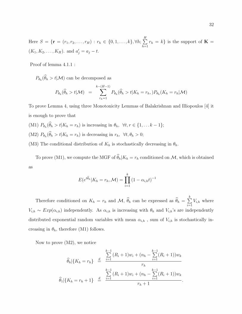
Proof of lemma 4.1.1 :

Pθh(θ̂h > t|M) can be decomposed as

Pθh(θ̂h > t|M) =

k−(H−1)∑rh=1

Pθh(θ̂h > t|Kh = rh, )Pθh(Kh = rh|M)

To prove Lemma 4, using three Monotonicity Lemmas of Balakrishnan and Illiopoulos [4] it

is enough to prove that

(M1) Pθh(θ̂h > t|Kh = rh) is increasing in θh, ∀t, r ∈ {1, . . . k − 1};

(M2) Pθh(θ̂h > t|Kh = rh) is decreasing in rh, ∀t, θh > 0;

(M3) The conditional distribution of Kh is stochastically decreasing in θh.

To prove (M1), we compute the MGF of θ̂h|Kh = rh conditioned onM, which is obtained

as

E(etθ̂h|Kh = rh,M) =k∏i=1

(1− αi,ht)−1

Therefore conditioned on Kh = rh and M, θ̂h can be expressed as θ̂h =k∑i=1

Vi,h where

Vi,h ∼ Exp(αi,h) independently. As αi,h is increasing with θh and Vi,h’s are independently

distributed exponential random variables with mean αi,h , sum of Vi,h is stochastically in-

creasing in θh, therefore (M1) follows.

Now to prove (M2), we notice

θ̂h|{Kh = rh}d=

k−1∑i=1

(Ri + 1)wi + (nh −k−1∑i=1

(Ri + 1))wk

rh

θ̂1|{Kh = rh + 1} d=

k−1∑i=1

(Ri + 1)wi + (nh −k−1∑i=1

(Ri + 1))wk

rh + 1.

33

Hence for all t and for θh > 0, Pθh(θ̂h > t|Kh = rh) is decreasing in rh.

(M3) can be proved showing that Kh has monotone likelihood ratio property with respect

to θh. For θh < θh′

Pθh(Kh = rh|M)

Pθh′(Kh = rh|M)∝(θh′θh

)rh↑ rh.

Appendix B

Proof of lemma 5.2.1:

If part:

Let X1, X2, . . . Xn be non-negative random variables such thatn∑i=1

Xi ∼ GA(a0, b0),

(X1n∑i=1

Xi

,X1n∑i=1

Xi

, . . . ,Xnn∑i=1

Xi

) ∼ D(a1, a2, . . . , an) and they are independently distributed.

We use the following notations,

T =n∑i=1

Xi; Yi =Xin∑i=1

Xi

for i = 1, . . . , n− 1.

Then the joint distribution of T, Y1, . . . , Yn−1 can be written as

fY1,...,Yn−1,T (t, y1, · · · , yn−1) ∝n−1∏i=1

yai−1i (1−

n−1∑i=1

yi)an−1ta0−1e−b0t.

Now the Xi’s can be written as

Xi = TYi for i = 1, . . . , n− 1, and Xn = T (1−n−1∑i=1

Yi).

To derive the joint distribution of (X1, . . . , Xn), we find out the Jacobian J where

J−1 =

∂X1

∂Y1

∂X1

∂Y2. . . ∂X1

∂Yn−1

∂X1

∂T∂X2

∂Y1

∂X2

∂Y2. . . ∂X2

∂Yn−1

∂X2

∂T...

... · · · ......

∂Xn∂Y1

∂Xn∂Y2

. . . ∂Xn∂Yn−1

∂Xn∂T

=

T 0 . . . 0 Y1

0 T . . . 0 Y2...

−T −T −T (1−n−1∑i=1

Yi)

.

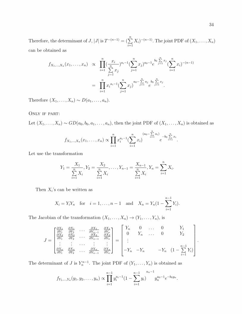
34

Therefore, the determinant of J , |J | is T−(n−1) = (n∑i=1

Xi)−(n−1). The joint PDF of (X1, . . . , Xn)

can be obtained as

fX1,...,Xn(x1, . . . , xn) ∝n∏i=1

(xin∑j=1

xj

)ai−1(n∑j=1

xj)a0−1e

b0n∑j=1

xj(n∑i=1

xi)−(n−1)

=n∏i=1

xiai−1(

n∑j=1

xj)a0−

n∑j=1

ajeb0

n∑j=1

xj.

Therefore (X1, . . . , Xn) ∼ D(a1, . . . , an).

Only if part:

Let (X1, . . . , Xn) ∼ GD(a0, b0, a1, . . . , an), then the joint PDF of (X1, . . . , Xn) is obtained as

fX1,...,Xn(x1, . . . , xn) ∝n∏i=1

xai−1i (

n∑i=1

xi)

(a0−n∑i=1

ai)

e−b0

n∑i=1

xi.

Let use the transformation

Y1 =X1n∑i=1

Xi

, Y2 =X2n∑i=1

Xi

, . . . , Yn−1 =Xn−1n∑i=1

Xi

, Yn =n∑i=1

Xi.

Then Xi’s can be written as

Xi = YiYn for i = 1, . . . , n− 1 and Xn = Yn(1−n−1∑i=1

Yi).

The Jacobian of the transformation (X1, . . . , Xn)→ (Y1, . . . , Yn), is

J =

∂X1

∂Y1

∂X1

∂Y2. . . ∂X1

∂Yn−1

∂X1

∂Yn∂X2

∂Y1

∂X2

∂Y2. . . ∂X2

∂Yn−1

∂X2

∂Yn...

... · · · ......

∂Xn∂Y1

∂Xn∂Y2

. . . ∂Xn∂Yn−1

∂Xn∂Yn

=

Yn 0 . . . 0 Y1

0 Yn . . . 0 Y2...

−Yn −Yn −Yn (1−n−1∑i=1

Yi)

.

The determinant of J is Y n−1n . The joint PDF of (Y1, . . . , Yn) is obtained as

fY1,...,Yn(y1, y2, . . . , yn) ∝n−1∏i=1

yai−1i (1−

n−1∑i=1

yi)

an−1

ya0−1n e−b0yn .

35

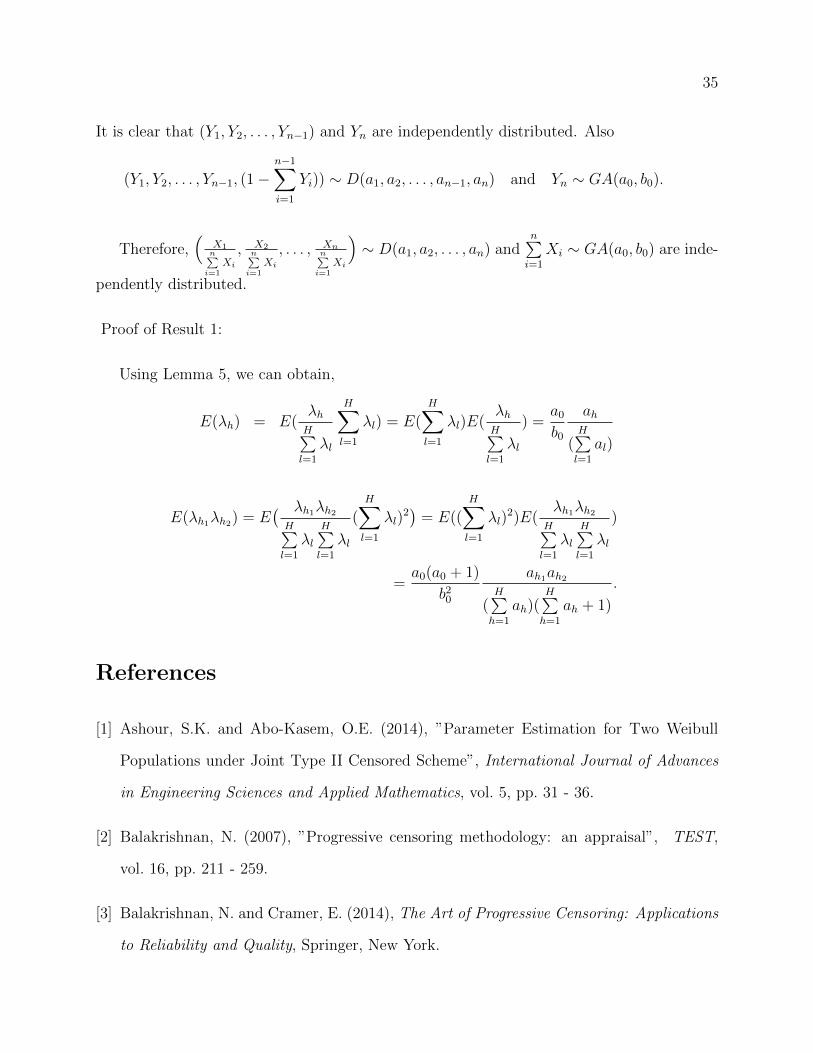
It is clear that (Y1, Y2, . . . , Yn−1) and Yn are independently distributed. Also

(Y1, Y2, . . . , Yn−1, (1−n−1∑i=1

Yi)) ∼ D(a1, a2, . . . , an−1, an) and Yn ∼ GA(a0, b0).

Therefore,(

X1n∑i=1

Xi

, X2n∑i=1

Xi

, . . . , Xnn∑i=1

Xi

)∼ D(a1, a2, . . . , an) and

n∑i=1

Xi ∼ GA(a0, b0) are inde-

pendently distributed.

Proof of Result 1:

Using Lemma 5, we can obtain,

E(λh) = E(λhH∑l=1

λl

H∑l=1

λl) = E(H∑l=1

λl)E(λhH∑l=1

λl

) =a0

b0

ah

(H∑l=1

al)

E(λh1λh2) = E( λh1λh2H∑l=1

λlH∑l=1

λl

(H∑l=1

λl)2)

= E((H∑l=1

λl)2)E(

λh1λh2H∑l=1

λlH∑l=1

λl

)

=a0(a0 + 1)

b20

ah1ah2

(H∑h=1

ah)(H∑h=1

ah + 1)

.

References

[1] Ashour, S.K. and Abo-Kasem, O.E. (2014), ”Parameter Estimation for Two Weibull

Populations under Joint Type II Censored Scheme”, International Journal of Advances

in Engineering Sciences and Applied Mathematics, vol. 5, pp. 31 - 36.

[2] Balakrishnan, N. (2007), ”Progressive censoring methodology: an appraisal”, TEST,

vol. 16, pp. 211 - 259.

[3] Balakrishnan, N. and Cramer, E. (2014), The Art of Progressive Censoring: Applications

to Reliability and Quality, Springer, New York.

36

[4] Balakrishnan, N. and Iliopoulos, G. (2009), ”Stochastic monotonicity of the MLE of

exponential mean under different censoring schemes”, Annals of the Institute of Statistical

Mathematics, vol. 61, pp. 753 - 772.

[5] Balakrishnan, N. and Rasouli, A. (2008), ”Exact likelihood inference for two exponential

populations under joint Type-II censoring”, Computational Statistics & Data Analysis,

vol. 52, pp. 2725 - 2738.

[6] Balakrishnan, N. and Su, F. (2015), ”Exact likelihood inference for k exponential pop-

ulations under joint type-II censoring”, Communications in Statistics - Simulation and

Computation, vol. 44, pp. 591 - 613.

[7] Balakrishnan N., Su F. and Liu K. Y. (2015), ”Exact Likelihood Inference for k Expo-

nential Populations Under Joint Progressive Type-II Censoring”, Communications in

Statistics - Simulation and Computation, vol. 44, pp. 902 - 923.

[8] Bartholmew, D. (1963), ”The sampling distribution of an estimate arising in life-testing”.

Technometrics, vol. 5, pp. 361 - 372.

[9] Casella, G., Berger, R. L. (2002). Statistical inference (2nd ed.) Boston: Duxbury Press.

[10] Kundu, D. and Pradhan, B. (2011), ”Bayesian analysis of progressively censored com-

peting risks data”, Sankhya B , vol. 73, pp. 276 - 296.

[11] Kundu, D., Samanta, D., Ganguly, A. and Mitra, S.(2013), ”Bayesian Analysis of Dif-

ferent Hybrid and Progressive Life Tests”, Communications in Statistics - Simulation

and Computation, vol. 42, pp. 2160 - 2173.

[12] Lehmann, E.L. and Romano, J.P. (2005), Testing Statistical Hypotheses Springer Texts

in Statistics, New York, Chapter-3.

37

[13] Mondal, S. and Kundu, D. (2018), ”A new two sample Type-II progres-

sive censoring scheme”, Communications in Statistics - Theory and Methods,

DOI:10.1080/03610926.2018.1472781.

[14] Mondal, S. and Kundu, D.(2017), ”Point and Interval Estimation of Weibull Parameters

Based on Joint Progressively Censored Data”, Sankhya B, DOI:10.1007/s13571-017-

0134-1.

[15] Nelson, W. (1982), Applied Life Data Analysis, John Wiley & Sons, New York.

[16] Parsi, S. and Bairamov, I. (2009), ”Expected values of the number of failures for two

populations under joint Type-II progressive censoring”, Computational Statistics & Data

Analysis, vol. 53, pp. 3560 - 3570.

[17] Parsi S., Ganjali M. and Sanjari F. N. (2011), ”Conditional Maximum Likelihood and

Interval Estimation for Two Weibull Populations under Joint Type-II Progressive Cen-

soring”, Communications in Statistics - Theory and Methods, vol. 40, pp. 2117 - 2135.

[18] Pena, E. A. and Gupta, A. K. (1990), ”Bayes estimation for the Marshall-Olkin expo-

nential distribution”, Journal of the Royal Statistical Society, vol. 52, pp. 379 - 389.

[19] Proschan, F. (1963), ”Theoretical explanation of observed decreasing failure rate”,

Technometrics, vol. 15, pp. 375 - 383.

[20] Rasouli, A. and Balakrishnan, N. (2010), “Exact likelihood inference for two exponential

populations under joint progressive type-II censoring”, Communications in Statistics -

Theory and Methods, vol. 39, pp. 2172 - 2191.

[21] Srivastava, J.N. (1987), “More efficient and less time-consuming censoring design for

testing”, Journal of Statistical Planning and Inference, vol. 16, 389 - 413.

38

Table 5: AE and MSE of the MLEs and BE and MSE of Bayes Estimators of θ1, θ2, θ3, θ4, θ5

based on informative prior (IP) and non-informative prior (NIP) with θ1 = 0.3, θ2 = 0.4, θ3 =0.5, θ4 = 0.6, θ5 = 0.7

sample sizes censoring scheme Parameter MLE Bayes IP Bayes NIPAE MSE BE MSE BE MSE

n1 = 15, n2 = 16, n3 = 15, n4 = 15, n5 = 16 k=8,R=( 2, 0(6)) θ1 0.453 0.092 0.394 0.032 0.626 0.283θ2 0.547 0.113 0.557 0.078 0.773 0.434θ3 0.548 0.080 0.779 0.212 0.914 0.547θ4 0.571 0.077 1.034 0.448 1.015 0.579θ5 0.645 0.090 1.336 0.990 1.034 0.512

n1 = 15, n2 = 15, n3 = 15, n4 = 15, n5 = 15 k=8,R=( 2, 0(6)) θ1 0.463 0.101 0.385 0.027 0.629 0.275θ2 0.525 0.097 0.557 0.078 0.781 0.392θ3 0.565 0.088 0.766 0.192 0.899 0.548θ4 0.590 0.084 1.007 0.395 0.999 0.567θ5 0.631 0.091 1.309 0.872 1.109 0.599

n1 = 25, n2 = 25, n3 = 25, n4 = 25, n5 = 25 k=20,R=( 5, 0(18)) θ1 0.351 0.041 0.353 0.014 0.436 0.069θ2 0.505 0.127 0.497 0.041 0.562 0.123θ3 0.645 0.210 0.667 0.108 0.724 0.253θ4 0.777 0.288 0.863 0.256 0.868 0.349θ5 0.881 0.344 1.106 0.585 0.969 0.446

k=20,R=( 0(18), 5) θ1 0.352 0.039 0.354 0.014 0.438 0.056θ2 0.504 0.124 0.494 0.040 0.589 0.138θ3 0.657 0.231 0.670 0.111 0.708 0.232θ4 0.776 0.288 0.893 0.283 0.851 0.357θ5 0.875 0.332 1.093 0.555 0.960 0.425

n1 = 25, n2 = 26, n3 = 27, n4 = 28, n5 = 29 k=20,R=(5, 0(18)) θ1 0.371 0.064 0.359 0.016 0.462 0.070θ2 0.510 0.133 0.502 0.043 0.598 0.135θ3 0.645 0.221 0.661 0.112 0.716 0.212θ4 0.773 0.316 0.831 0.226 0.824 0.307θ5 0.906 0.417 0.998 0.386 0.925 0.349

k=20, R=(0(18), 5) θ1 0.364 0.054 0.350 0.014 0.475 0.100θ2 0.505 0.132 0.489 0.042 0.577 0.136θ3 0.650 0.220 0.662 0.101 0.711 0.223θ4 0.780 0.312 0.874 0.280 0.815 0.273θ5 0.909 0.415 1.023 0.410 0.922 0.424

n1 = 30, n2 = 30, n3 = 30, n4 = 30, n5 = 30 k=25,R=(5, 0(23)) θ1 0.341 0.030 0.393 0.011 0.406 0.034θ2 0.482 0.094 0.489 0.036 0.552 0.094θ3 0.635 0.198 0.640 0.088 0.676 0.153θ4 0.782 0.317 0.812 0.198 0.798 0.251θ5 0.904 0.408 1.051 0.552 0.923 0.375

k=25,R=(0(23), 5) θ1 0.338 0.032 0.346 0.013 0.412 0.046θ2 0.486 0.103 0.490 0.039 0.543 0.112θ3 0.637 0.210 0.643 0.090 0.680 0.107θ4 0.774 0.309 0.825 0.215 0.809 0.278θ5 0.901 0.405 1.062 0.523 0.941 0.412

39

Table 6: AL and CP of the 90% Exact and Percentile Bootstrap CI of θ1, θ2, θ3, θ4, θ5 withθ1 = 0.3, θ2 = 0.4, θ3 = 0.5, θ4 = 0.6, θ5 = 0.7

sample sizes censoring scheme Parameter 90% Bootstrap CI 90% Exact CIAL CP AL CP

n1 = 15, n2 = 16, n3 = 15, n4 = 15, n5 = 16 k=8,R=(2, 0(6)) θ1 0.847 94.1% 1.967 94.0%θ2 0.952 97.2% 2.121 96.1%θ3 0.873 95.1% 2.412 96.5%θ4 0.875 89.9% 2.609 94.8%θ5 0.976 88.4% 2.251 93.3%

n1 = 15, n2 = 15, n3 = 15, n4 = 15, n5 = 15 k=8,R=(2, 0(6)) θ1 0.850 94.1% 1.748 95.6%θ2 0.873 97.2% 1.971 94.7%θ3 0.881 95.2% 1.992 93.9%θ4 0.887 91.8% 2.170 91.1%θ5 0.889 86.5% 2.175 95.8%

n1 = 25, n2 = 25, n3 = 25, n4 = 25, n5 = 25 k=20,R=(5, 0(18)) θ1 0.716 91.0% 0.771 92.7%θ2 1.105 89.6% 1.601 96.0%θ3 1.417 88.2% 2.072 92.1%θ4 1.525 91.7% 2.909 95.1%θ5 1.627 95.0% 3.344 94.2%

k=20,R=( 0(18), 5) θ1 0.718 91.2% 0.686 92.0%θ2 1.096 90.3% 1.646 94.6%θ3 1.337 91.1% 2.243 94.6%θ4 1.527 93.4% 3.061 95.1%θ5 1.597 95.9% 2.641 90.5%

n1 = 30, n2 = 30, n3 = 30, n4 = 30, n5 = 30 k=25,R=(5, 0(23)) θ1 0.608 89.3% 0.531 91.0%θ2 1.039 88.1% 0.925 94.8%θ3 1.316 89.9% 1.422 95.7%θ4 1.590 90.1% 2.288 94.1%θ5 1.748 89.9% 2.100 93.7%

k=25,R=( 0(23), 5) θ1 0.620 88.1% 0.518 93.0%θ2 1.019 90.7% 0.923 94.9%θ3 1.365 90.0% 0.923 94.9%θ4 1.583 904% 2.013 96.5%θ5 1.723 90.3% 2.761 94.6%

40

Table 7: AL and CP of the 90% HPD credible interval (H-CRI) and Symmetric credibleinterval (S-CRI) of θ1, θ2, θ3, θ4, θ5 based on informative prior (IP) and non-informative prior(NIP) with θ1 = 0.3, θ2 = 0.4, θ3 = 0.5, θ4 = 0.6, θ5 = 0.7

sample sizes censoring scheme Parameter 90% H-CRI 90% S-CRIIP NIP IP NIP

AL CP AL CP AL CP AL CP

n1 = 15, n2 = 16, n3 = 15, n4 = 15, n5 = 16 k=8,R=(2, 0(6)) θ1 0.527 96.8% 1.067 95.4% 0.626 97.2% 1.336 88.9%θ2 0.845 97.4% 1.221 96.2% 1.003 97.9% 1.645 94.9%θ3 1.277 97.8% 1.634 95.0% 1.601 96.8% 2.251 95.6%θ4 1.750 98.0% 1.822 93.2% 2.361 98.4% 2.537 96.4%θ5 2.271 97.8% 1.814 94.2% 2.178 97.9% 2.516 95.4%

n1 = 15, n2 = 15, n3 = 15, n4 = 15, n5 = 15 k=8,R=( 2, 0(6) ) θ1 0.536 97.0% 1.030 97.4% 0.614 95.9% 1.330 87.6%θ2 0.820 96.5% 1.315 96.6% 1.004 96.3% 1.784 93.3%θ3 1.246 97.6% 1.530 97.0% 1.547 94.4% 2.137 94.9%θ4 1.692 97.1% 1.723 95.2% 2.251 97.3% 2.497 97.5%θ5 2.281 97.2% 1.876 92.2% 2.231 97.6% 2.632 96.0%

n1 = 25, n2 = 25, n3 = 25, n4 = 25, n5 = 25 k=20,R=(5, 0(18)) θ1 0.376 96.9% 0.530 93.6% 0.421 92.8% 0.611 89.4%θ2 0.591 95.5% 0.774 96.4% 0.676 94.4% 0.948 92.3%θ3 0.886 94.7% 1.009 93.0% 1.035 95.4% 1.319 93.2%θ4 1.222 95.7% 1.281 95.0% 1.538 93.9% 1.628 93.9%θ5 1.780 95.1% 1.436 92.8% 2.113 95.4% 1.866 94.2%

k=20,R=(0(18), 5) θ1 0.369 93.2% 0.516 94.8% 0.408 95.6% 0.603 88.4%θ2 0.580 96.2% 0.783 94.8% 0.690 93.8% 0.905 93.8%θ3 0.879 97.0% 1.009 96.2% 1.045 94.4% 1.283 92.9%θ4 1.206 96.2% 1.147 92.4% 1.506 95.2% 1.564 94.8%θ5 1.668 96.2% 1.507 91.4% 2.219 95.0% 1.905 95.2%

n1 = 25, n2 = 26, n3 = 27, n4 = 28, n5 = 29 k=20, R=(5, 0(18)) θ1 0.393 95.6% 0.582 95.0% 0.444 95.6% 0.744 89.2%θ2 0.599 94.4% 0.845 94.6% 0.716 96.0% 1.032 91.4%θ3 0.826 96.2% 0.939 95.0% 1.026 94.9% 1.228 93.2%θ4 1.164 96.8% 1.162 91.6% 1.429 93.5% 1.503 94.3%θ5 1.365 95.0% 1.280 89.8% 1.807 94.2% 1.692 93.8%

k=20, R=(0(18), 5) θ1 0.388 94.6% 0.590 93.8% 0.426 96.2% 0.712 87.1%θ2 0.575 93.8% 0.826 93.8% 0.707 94.8% 0.982 93.2%θ3 0.890 97.6% 0.991 94.0% 1.033 95.7% 1.237 94.8%θ4 1.186 96.0% 1.208 93.6% 1.391 94.2% 1.498 94.2%θ5 1.591 95.4% 1.300 91.8% 1.942 94.2% 1.779 93.9%

n1 = 30, n2 = 30, n3 = 30, n4 = 30, n5 = 30 k=25, R=(5, 0(23)) θ1 0.333 94.2% 0.456 94.8% 0.368 93.8% 0.522 88.2%θ2 0.533 95.0% 0.674 94.6% 0.605 94.4% 0.760 92.3%θ3 0.790 95.8% 0.898 93.9% 0.904 93.5% 1.091 92.7%θ4 1.098 96.2% 1.073 91.8% 1.331 93.6% 1.342 95.3%θ5 1.534 94.8% 1.359 90.8% 1.823 94.3% 1.654 92.9%

k=25, R=(0(23), 5) θ1 0.337 94.6% 0.443 96.6% 0.358 95.2% 0.504 89.6%θ2 0.543 96.1% 0.663 94.6% 0.609 92.4% 0.759 92.5%θ3 0.784 96.1% 0.927 96.4% 0.918 93.1% 1.143 90.9%θ4 1.093 95.8% 1.125 93.4% 1.317 95.5% 1.373 94.0%θ5 1.510 95.4% 1.335 92.0% 1.887 94.3% 1.667 93.5%