Exact Cardinality Query Optimization for Optimizer Testing Surajit Chaudhuri

surajitc@microsoft.com Vivek Narasayya

viveknar@microsoft.com Ravi Ramamurthy

ravirama@microsoft.com

ABSTRACT

The accuracy of cardinality estimates is crucial for obtaining a

good query execution plan. Today‟s optimizers make several

simplifying assumptions during cardinality estimation that can

lead to large errors and hence poor plans. In a scenario such as

query optimizer testing it is very desirable to obtain the “best”

plan, i.e., the plan produced when the cardinality of each relevant

expression is exact. Such a plan serves as a baseline against which

plans produced by using the existing cardinality estimation

module in the query optimizer can be compared. However,

obtaining all exact cardinalities by executing appropriate sub-

expressions can be prohibitively expensive. In this paper, we

present a set of techniques that makes exact cardinality query

optimization a viable option for a significantly larger set of

queries than previously possible. We have implemented this

functionality in Microsoft SQL Server and we present results

using the TPC-H benchmark queries that demonstrate their

effectiveness.

1. INTRODUCTION Query optimizers rely on a cost model to choose an appropriate

query execution plan for a query. A key parameter of cost

estimation is the cardinality of sub-expressions of the query

considered during optimization. Obtaining accurate cardinality

estimates for these sub-expressions can be crucial for finding a

good query execution plan.

In an effort to keep the optimization time low, today‟s query

optimizers trade accuracy of cardinality estimation and hence

quality of execution plan. The time needed for query optimization

is kept low by using estimation techniques such as histograms to

obtain cardinalities of expressions. However, these estimation

techniques can lead to estimation errors. For example, it is well

known [14] that cardinality estimation errors can grow

exponentially in the number of joins in a query. This can cause the

optimizer to pick a plan that is significantly worse than the plan

that uses exact cardinalities for the sub-expressions. It is important

to understand to what extent the plan quality is affected by errors

in cardinality estimation. To do so, we need to obtain the “best”

plan (i.e. plan obtained using exact cardinalities) even if query

optimization time is considerably larger. Indeed, there are

important scenarios in query optimizer testing where the presence

of the best plan can be extremely valuable.

First, such a plan serves as a benchmark against which plans

produced by the current optimizer (using its built-in cardinality

estimation module) can be compared. Second, it can also help

narrow down the cause of a plan quality problem. For example,

consider the case of a particular transformation rule in the

optimizer [12]. Suppose that the rule was expected to improve the

efficiency of a particular query but in reality did not. Today it is

difficult to know if this was due to poor cardinality estimation or a

different problem (e.g. issues in the search strategy or other cost

parameters). Being able to obtain the plan without any cardinality

estimation errors can help resolve the above question. Third, once

exact cardinalities are available, we can analyze whether the plan

obtained when using exact cardinalities for all expressions is

identical to the plan obtained when using exact cardinalities for

only a subset of sub-expressions e.g., for leaf (i.e. single-table)

expressions. Such analysis could be useful in isolating classes of

expressions for which estimation errors can have a significant

impact on plan quality.

In this paper, we study the exact cardinality query optimization

problem, i.e. optimizing the query using the exact cardinality for

each relevant expression. A relevant expression is one whose

cardinality is required during optimization. Since the time for

exact cardinality query optimization can be significant, improving

its efficiency can be valuable. Specifically, the natural approach

of executing one query per relevant expression to obtain its

cardinality can be prohibitively expensive since: (a) there can be a

large number of relevant expressions for a query, and (b) the total

time taken to execute all these queries can be significant.

Example 1. Consider the following query on the TPC-H database.

SELECT … FROM Lineitem, Orders, Customer

WHERE l_orderkey = o_orderkey

AND o_custkey = c_custkey

AND l_shipdate > „2008-01-01‟

AND l_receiptdate < „2008-02-01‟

AND l_discount < 0.05

AND o_orderpriority = „HIGH‟

AND c_mktsegment = „AUTOMOBILE‟

Suppose we have single column indexes on (l_shipdate) and

(l_receipdate) in the database. The expressions whose

cardinalities are considered by a typical query optimizer consist of

the following 6 single-table expressions and 3 join expressions.

For simplicity, we do not indicate the predicates in the join

expressions:

(1) (l_shipdate > „2008-01-01‟)

(2) (l_receiptdate < „2008-02-01‟)

(3) (l_shipdate > „2008-01-01‟ AND l_receiptdate < „2008-02-

01‟)

Permission to copy without fee all or part of this material is granted provided

that the copies are not made or distributed for direct commercial advantage, the VLDB copyright notice and the title of the publication and its date

appear, and notice is given that copying is by permission of the Very Large

Database Endowment. To copy otherwise, or to republish, to post on servers

or to redistribute to lists, requires a fee and/or special permissions from the

publisher, ACM.

VLDB ’09, August 24-28, 2009, Lyon, France.

Copyright 2009 VLDB Endowment, ACM 000-0-00000-000-0/00/00.

(4) (l_shipdate > „2008-01-01‟ AND l_receiptdate < „2008-02-

01‟ AND l_discount < 0.05)

(5) (o_orderpriority = „HIGH‟)

(6) (c_mktsegment = „AUTOMOBILE‟)

(7) (Customer Orders)

(8) (Orders Lineitem)

(9) (Lineitem Orders Customer)

Thus, the naïve approach for exact cardinality query optimization

requires executing1 each of the above nine expressions to obtain

the respective cardinalities and this can be expensive.

In this paper, we propose the exact cardinality query optimization

problem and present techniques that can significantly reduce the

time taken for such optimization. We leverage the key observation

that when an expression is executed, we can obtain cardinalities of

other related expressions as a byproduct. This is because each

physical operator in an execution plan can output its cardinality at

the end of execution, and the sub-tree rooted at an operator in the

plan also corresponds to a relevant sub-expression. Thus, in order

to compute the accurate values of all the required cardinalities for

the query, we only need to execute a subset of relevant

expressions of the query such that their execution results in

obtaining the complete set of all relevant cardinalities. We refer to

this as the Covering Queries optimization.

The exact cardinality query optimization functionality in general,

can also be invoked with a workload (i.e. set of queries) as input.

Indeed, in query optimizer testing, it is common to use a workload

of benchmark queries and real world customer queries. In such

cases, we need to obtain the exact cardinalities for the relevant

expressions of all the queries in the workload. While the

technique of materializing common sub-expressions to speed up

execution has been studied in the context of multi-query

optimization problem (MQO), e.g. [18][19], the fact that we are

interested only in the cardinalities (and not the actual results) of

expressions, offers unique opportunities that cannot be leveraged

in a general MQO setting. Specifically, as we will show, we can

take full advantage of common sub-expressions in the workload

but without the need for materialization and thus gain advantage

over known techniques in MQO. In particular, we leverage the

CASE statement in SQL which allows multiple count expressions

to be computed over a relation in a single pass without

materialization.

We have prototyped the exact cardinality query optimization

functionality in Microsoft SQL Server. This includes the Covering

Queries optimization as well as our technique for obtaining

cardinalities of common sub-expressions using appropriate CASE

queries. We have evaluated the effectiveness of our techniques on

TPC-H benchmark queries [22]. Our experiments demonstrate

significant speedups using our techniques relative to the baseline

approach of executing each relevant expression. While not the

main focus of the paper, we also show a few examples of

analytics for query optimizer testing that are possible once exact

cardinalities of relevant expressions are available.

The rest of the paper is structured as follows. In Section 2, we

describe the exact cardinality query optimization problem and

outline the architecture of our solution. Sections 3 and 4

1 Note that we only need to execute a COUNT(*) query

corresponding to each expression

respectively present the key technical ideas of Covering Queries

optimization and generation of CASE queries for a workload to

speed up exact cardinality query optimization. Section 5 presents

results of our experimental evaluation and we discuss related

work in Section 6.

2. PROBLEM STATEMENT

2.1 Preliminaries Query optimizer: A key input to the cost model of a query

optimizer is the cardinality of relevant logical sub-expressions2 of

the query. The query optimizer considers a set of sub-expressions

of the given query during optimization. In this paper, we use

Microsoft SQL Server, whose optimizer is based on the Cascades

framework [12] which maintains a memo data structure. Each

node in the memo is a group, which represents a logical

expression. Expressions in the memo are related to one another by

parent-child relationships, which indicate that the child is an input

to the parent expression. We present our techniques in the context

of an optimizer based on the Cascades framework [12], but the

techniques are potentially applicable to other optimizer

architectures as well.

Relevant Expressions for a Query: For any input query, the

optimizer considers a set of plans S. For any plan P S, there is a

set of logical expressions LE(P) whose cardinalities are necessary

for deriving the cost of plan P. The set of relevant expressions of a

query is defined to be the union of LE(P) over all plans in S. Note

that the set of relevant expressions for the same query could

potentially be different for different optimizers. For the Cascades

framework [12], the relevant expressions would be the set of

groups in the memo that correspond to relational expressions. For

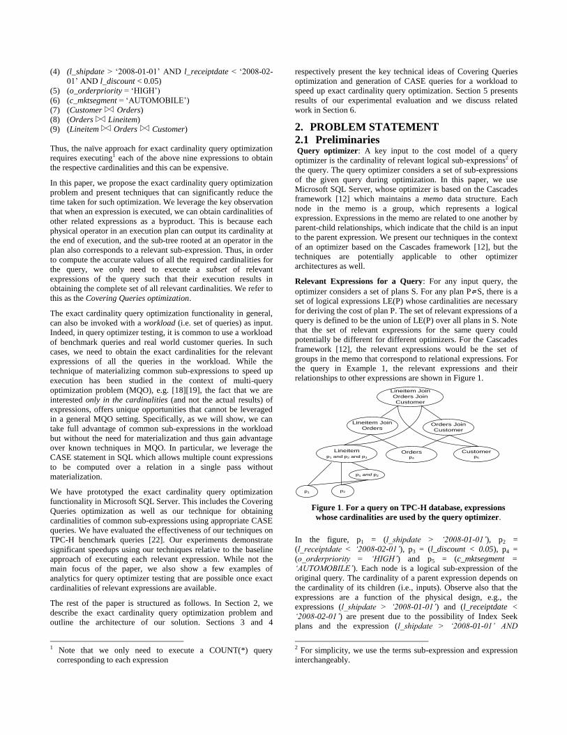
the query in Example 1, the relevant expressions and their

relationships to other expressions are shown in Figure 1.

Lineitem

p1 and p2 and p3

Orders Join

Customer

Lineitem Join

Orders

Customerp5

Ordersp4

Lineitem Join

Orders Join

Customer

p1 and p2

p1 p2

In the figure, p1 = (l_shipdate > ‘2008-01-01’), p2 =

(l_receiptdate < ‘2008-02-01’), p3 = (l_discount < 0.05), p4 =

(o_orderpriority = ‘HIGH’) and p5 = (c_mktsegment =

‘AUTOMOBILE’). Each node is a logical sub-expression of the

original query. The cardinality of a parent expression depends on

the cardinality of its children (i.e., inputs). Observe also that the

expressions are a function of the physical design, e.g., the

expressions (l_shipdate > ‘2008-01-01’) and (l_receiptdate <

‘2008-02-01’) are present due to the possibility of Index Seek

plans and the expression (l_shipdate > ‘2008-01-01’ AND

2 For simplicity, we use the terms sub-expression and expression

interchangeably.

Figure 1. For a query on TPC-H database, expressions

whose cardinalities are used by the query optimizer.

l_receiptdate < ‘2008-02-01’) is present due to the possibility of

an Index Intersection plan.

Observe that the above notion of relevant sub-expressions that

correspond to groups in the memo applies for any query,

including complex queries (e.g. with nested sub-queries).

Cardinality Estimation: Today‟s query optimizers rely on

summary statistics such as a histogram of the column values and

the number of distinct values in a column. Since DBMSs do not

typically maintain multi-column statistics or statistics on views,

when an expression has multiple predicates, optimizers resort to

simplifying assumptions such as independence between predicates

and containment (for joins) to estimate expression cardinality. As

a consequence, the errors in cardinality estimation can become

significant [14] leading to poor choice of execution plan.

Cardinality-optimal Plan: For a given query optimizer, one

important reason for suboptimal plan choices is inaccurate

cardinality estimates. We refer to the execution plan obtained

when the exact cardinality is used for each relevant expression as

the cardinality-optimal plan for the query.

Workload: For a given query Q, we denote the set of all relevant

expressions for the query by RQ. We define a workload W to be a

set of SQL queries. The set of relevant expressions for a workload

is the union of relevant expressions of all queries in the workload,

i.e. RW = Q W RQ.

Exact Cardinality Query Optimization Problem: The goal of

the exact cardinality query optimization problem is to find the

cardinality-optimal plan as quickly as possible. Note that the

output is required to be the cardinality-optimal plan. The problem

can be extended to take as input a workload of queries W and

return the cardinality-optimal plan for all the queries in the

workloads.

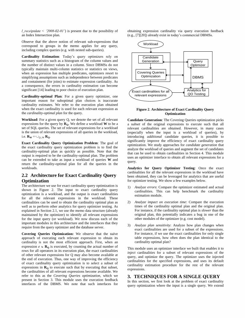
2.2 Architecture for Exact Cardinality Query

Optimization The architecture we use for exact cardinality query optimization is

shown in Figure 2. The input to exact cardinality query

optimization is a workload, and the output is exact cardinalities

for all the relevant expressions in the workload. These

cardinalities can be used to obtain the cardinality optimal plan as

well as to perform other analytics for query optimizer testing. As

explained in Section 2.1, we use the memo data structure (already

maintained by the optimizer) to identify all relevant expressions

for the input query (or workload). We now discuss each of the

important modules in this architecture and the interfaces that they

require from the query optimizer and the database server.

Covering Queries Optimization: We observe that the naïve

approach of executing each relevant expression to obtain its

cardinality is not the most efficient approach. First, when an

expression e RQ is executed, by counting the actual number of

rows for all operators in its execution plan, the exact cardinalities

of other relevant expressions for Q may also become available at

the end of execution. Thus, one way of improving the efficiency

of exact cardinality query optimization is to select a subset of

expressions in RQ to execute such that by executing that subset,

the cardinalities of all relevant expressions become available. We

refer to this as the Covering Queries optimization, which we

present in Section 3. This module uses the execution feedback

interfaces of the DBMS. We note that such interfaces for

obtaining expression cardinality via query execution feedback

(e.g., [7][20]) already exist in today‟s commercial DBMSs.

Workload

Candidate

Generation

Covering Queries

Optimization

Exact cardinalities for all

relevant expressions

Analytics for

QO Testing

DBMS

Query

Optimizer

Candidate Generation: The Covering Queries optimization picks

a subset of the original expressions to execute such that all

relevant cardinalities are obtained. However, in many cases

(especially when the input is a workload of queries), by

introducing additional candidate queries, it is possible to

significantly improve the efficiency of exact cardinality query

optimization. We study approaches for candidate generation that

analyze the workload of queries and augment the set of candidates

that can be used to obtain cardinalities in Section 4. This module

uses an optimizer interface to obtain all relevant expressions for a

query.

Analytics for Query Optimizer Testing: Once the exact

cardinalities for all the relevant expressions in the workload have

been obtained, they can be leveraged for analytics that are useful

for optimizer testing. We show a few examples below.

1) Analyze errors: Compare the optimizer estimated and actual

cardinalities. This can help benchmark the cardinality

estimation module.

2) Analyze impact on execution time: Compare the execution

times of the cardinality optimal plan and the original plan.

For instance, if the cardinality optimal plan is slower than the

original plan, this potentially indicates a bug in one of the

other modules of the optimizer (e.g. cost model).

3) Analyze plan sensitivity: Analyze how plan changes when

exact cardinalities are used for a subset of the expressions.

For instance, if we use the exact cardinalities for only single

table expressions, how often does the plan identical to the

cardinality optimal plan?

This module uses an optimizer interface we built that enables it to

inject cardinalities for a subset of relevant expressions of the

query, and optimize the query. The optimizer uses the injected

cardinalities for the specified expressions, and uses its default

cardinality estimation procedure for the rest of the relevant

expressions.

3. TECHNIQUES FOR A SINGLE QUERY In this section, we first look at the problem of exact cardinality

query optimization where the input is a single query. We extend

Figure 2. Architecture of Exact Cardinality Query

Optimization

our techniques to work for a workload of queries in Section 4. As

discussed earlier, the goal of the exact cardinality query

optimization problem is to obtain the cardinalities of all relevant

expressions as quickly as possible. The naïve approach is to

execute each expression in RQ and thus obtain its cardinality.

However, we observe that as a by-product of executing an

expression e in RQ, we can in fact obtain the cardinalities of other

expressions in RQ as well. Thus, we potentially do not need to

execute all expressions in RQ in order to obtain cardinalities of all

expressions in RQ.

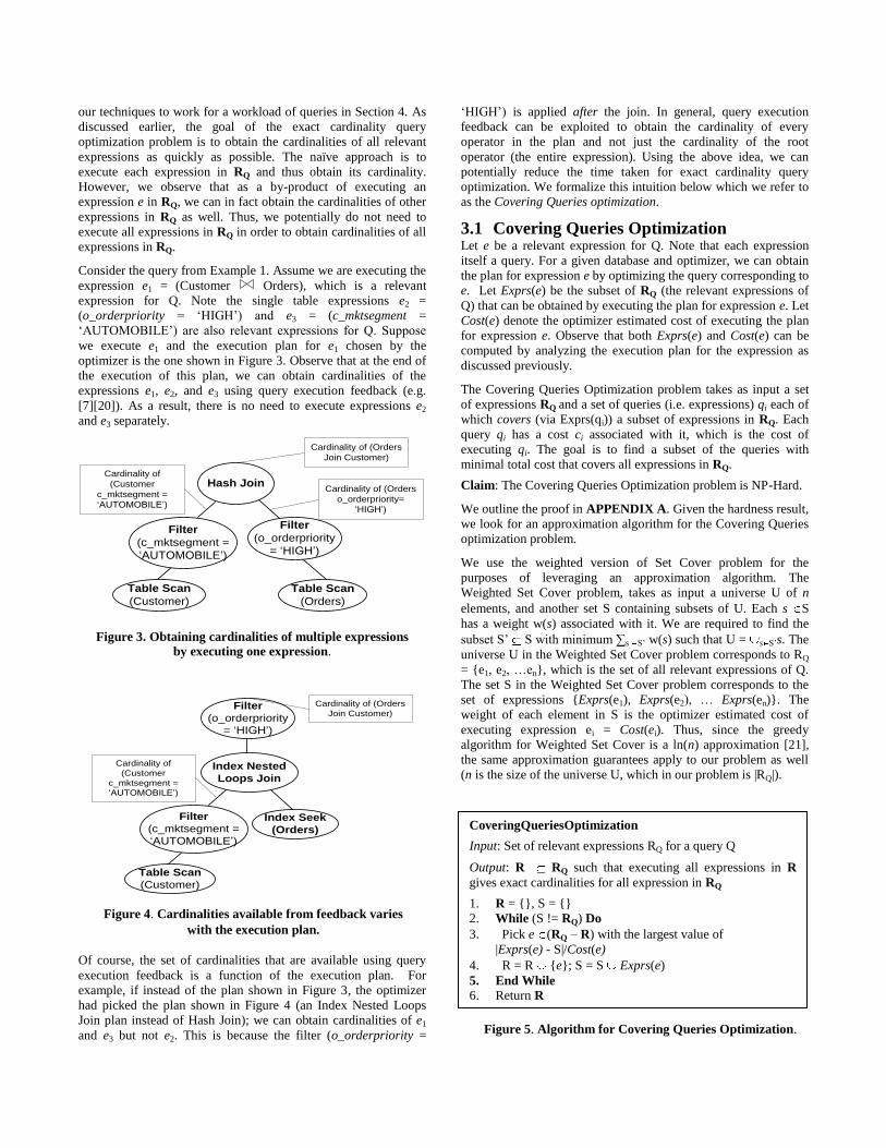
Consider the query from Example 1. Assume we are executing the

expression e1 = (Customer Orders), which is a relevant

expression for Q. Note the single table expressions e2 =

(o_orderpriority = „HIGH‟) and e3 = (c_mktsegment =

„AUTOMOBILE‟) are also relevant expressions for Q. Suppose

we execute e1 and the execution plan for e1 chosen by the

optimizer is the one shown in Figure 3. Observe that at the end of

the execution of this plan, we can obtain cardinalities of the

expressions e1, e2, and e3 using query execution feedback (e.g.

[7][20]). As a result, there is no need to execute expressions e2

and e3 separately.

Table Scan

(Customer)

Table Scan

(Orders)

Hash Join

Filter

(c_mktsegment =

‘AUTOMOBILE’)

Filter

(o_orderpriority

= ‘HIGH’)

Cardinality of (Orders

o_orderpriority=

‘HIGH’)

Cardinality of

(Customer

c_mktsegment =

‘AUTOMOBILE’)

Cardinality of (Orders

Join Customer)

Table Scan

(Customer)

Index Seek

(Orders)

Index Nested

Loops Join

Filter

(c_mktsegment =

‘AUTOMOBILE’)

Filter

(o_orderpriority

= ‘HIGH’)

Cardinality of

(Customer

c_mktsegment =

‘AUTOMOBILE’)

Cardinality of (Orders

Join Customer)

Of course, the set of cardinalities that are available using query

execution feedback is a function of the execution plan. For

example, if instead of the plan shown in Figure 3, the optimizer

had picked the plan shown in Figure 4 (an Index Nested Loops

Join plan instead of Hash Join); we can obtain cardinalities of e1

and e3 but not e2. This is because the filter (o_orderpriority =

„HIGH‟) is applied after the join. In general, query execution

feedback can be exploited to obtain the cardinality of every

operator in the plan and not just the cardinality of the root

operator (the entire expression). Using the above idea, we can

potentially reduce the time taken for exact cardinality query

optimization. We formalize this intuition below which we refer to

as the Covering Queries optimization.

3.1 Covering Queries Optimization Let e be a relevant expression for Q. Note that each expression

itself a query. For a given database and optimizer, we can obtain

the plan for expression e by optimizing the query corresponding to

e. Let Exprs(e) be the subset of RQ (the relevant expressions of

Q) that can be obtained by executing the plan for expression e. Let

Cost(e) denote the optimizer estimated cost of executing the plan

for expression e. Observe that both Exprs(e) and Cost(e) can be

computed by analyzing the execution plan for the expression as

discussed previously.

The Covering Queries Optimization problem takes as input a set

of expressions RQ and a set of queries (i.e. expressions) qi each of

which covers (via Exprs(qi)) a subset of expressions in RQ. Each

query qi has a cost ci associated with it, which is the cost of

executing qi. The goal is to find a subset of the queries with

minimal total cost that covers all expressions in RQ.

Claim: The Covering Queries Optimization problem is NP-Hard.

We outline the proof in APPENDIX A. Given the hardness result,

we look for an approximation algorithm for the Covering Queries

optimization problem.

We use the weighted version of Set Cover problem for the

purposes of leveraging an approximation algorithm. The

Weighted Set Cover problem, takes as input a universe U of n

elements, and another set S containing subsets of U. Each s S

has a weight w(s) associated with it. We are required to find the

subset S‟ S with minimum ∑s S‟ w(s) such that U = s S‟s. The

universe U in the Weighted Set Cover problem corresponds to RQ

= {e1, e2, …en}, which is the set of all relevant expressions of Q.

The set S in the Weighted Set Cover problem corresponds to the

set of expressions {Exprs(e1), Exprs(e2), … Exprs(en)}. The

weight of each element in S is the optimizer estimated cost of

executing expression ei = Cost(ei). Thus, since the greedy

algorithm for Weighted Set Cover is a ln(n) approximation [21],

the same approximation guarantees apply to our problem as well

(n is the size of the universe U, which in our problem is |RQ|).

Figure 4. Cardinalities available from feedback varies

with the execution plan.

Figure 5. Algorithm for Covering Queries Optimization.

CoveringQueriesOptimization

Input: Set of relevant expressions RQ for a query Q

Output: R RQ such that executing all expressions in R

gives exact cardinalities for all expression in RQ

1. R = {}, S = {}

2. While (S != RQ) Do

3. Pick e (RQ – R) with the largest value of

|Exprs(e) - S|/Cost(e)

4. R = R {e}; S = S Exprs(e)

5. End While

6. Return R

Figure 3. Obtaining cardinalities of multiple expressions

by executing one expression.

In Figure 5, we outline our algorithm for the Covering Queries

Optimization problem for the case of a single query, which uses

the greedy heuristic for Weighted Set Cover. Note that for the

single query case, the set of queries is initialized to the set of

relevant expressions RQ. We discuss how we can augment this set

for the workload case by generating additional candidates in

Section 4. In Step 4 we pick the expression with the largest ratio

of |Exprs(e) – S| / Cost(e); thus the numerator only counts

expressions that can be obtained by executing e that are not

already in S. The above algorithm outputs a set of expressions R

such that by executing those expressions we can obtain exact

cardinalities for all relevant expressions of Q. Our experiments

(Section 5) show that the Covering Queries Optimization can

significantly reduce the time needed for exact cardinality query

optimization.

4. TECHNIQUES FOR A WORKLOAD OF

QUERIES Commercial query optimizers are typically tested using a wide

variety of workloads that include well known benchmarks (such

as TPC-H) as well as real world workloads obtained from

customers. Recall from Section 2 that we define a workload W as

a set of SQL queries; and the set of relevant expressions for a

workload is the union of relevant expressions of all queries in the

workload, i.e. RW = Q W RQ. The Covering Queries algorithm,

presented in Section 3 for the case of a single query, can be

generalized in a straightforward manner for a workload. The

algorithm in Figure 5 can be used with RW as input and would

find a subset to execute such that we obtain cardinalities of all

expressions in RW. Note that this extension of the algorithm can

be quite effective for cases where multiple queries share identical

relevant expressions. However, this approach has limitations as

illustrated by the following example.

Example 2. Consider the following two similar (but not identical)

relevant expressions e1 and e2:

e1 = SELECT … FROM Lineitem

WHERE l_discount < 0.05 and

l_shipdate < ‘1998-01-01’

e2 = SELECT … FROM Lineitem

WHERE l_discount < 0.15 and

l_shipdate < ‘1997-01-01’

Since these expressions are not identical, the Covering Queries

algorithm would need to execute both expressions e1 and e2. This

example points to an opportunity to improve the performance of

exact cardinality query optimization by exploiting commonality

across relevant expressions for the workload. Many benchmark

and real world workloads consist of “templatized” queries that are

identical except for constants in the selection conditions. For such

workloads, leveraging commonality of relevant expressions across

queries in the workload can be very important.

4.1 Motivating use of CASE statement for

obtaining multiple expression cardinalities One way to exploit commonality across relevant expressions for a

workload is to use materialized views. Physical database design

tools in most commercial DBMSs (e.g. [2][3][24]) can

recommend appropriate materialized views for a workload.

However, such tools were designed to optimize performance of

workloads without accounting for the cost of materializing these

structures or the time taken to tune the workload as part of their

optimization. While these assumptions are reasonable for the

physical design problem, applying such tools directly can be

inappropriate for our problem.

We observe that the exact cardinality query optimization problem

for a workload is related to the multi-query optimization problem

(e.g. [18][19]) for the set RW. In multi-query optimization, a set of

common sub-expressions is first materialized, and the queries are

then executed using the materialized sub-expressions. Speedup in

execution can occur since the common sub-expression needs to be

executed (and materialized) only once; but can be reused for

executing multiple queries in RW. In the context of Example 2,

using the above approach, we could potentially materialize a sub-

expression such as:

SELECT l_shipdate, l_discount

FROM Lineitem

WHERE l_discount < 0.15 and l_shipdate <

‘1998-01-01’

The two relevant expressions e1 and e2 of Example 2 could then

be rewritten to use the materialized result.

However, we observe that in our problem, the expressions in RW

have a specific property. Since we require the cardinality of

relevant expressions, we only need the count of the number of

rows in the result of the expression (and do not need the actual

result of the expression). For this class of expressions, we

observe that it is possible to obtain cardinalities of multiple

expressions without need for materialization. In particular, we

leverage the fact that the CASE construct in SQL allows

computing multiple expressions on a relation in a single pass. For

example, the cardinalities of e1 and e2 in Example 2 can be

obtained using the following query that uses the CASE construct.

SELECT SUM(a) as card1, SUM(b) as card2

FROM

(

SELECT a = CASE when (l_discount < 0.05

and l_shipdate< ‘1998-01-01’) then

1 else 0 end,

b = CASE when (l_discount < 0.15

and l_shipdate < ‘1997-01-01’) then

1 else 0 end

FROM Lineitem

WHERE l_discount < 0.15 and

l_shipdate < ‘1998-01-01’

)

In certain cases (e.g. if executing each of the relevant expressions

requires a Scan of the Lineitem table), the new query may

execute faster than the combined execution times of e1 and e2. The

above example shows why CASE queries can be an effective

mechanism for obtaining cardinalities of relevant expressions.

We note that there has also been work on multi-query

optimization where materialization is not required [8]. However,

this assumes the availability of an execution engine that can

support DAG plans (to facilitate reuse of sub-expressions). Such

support is typically not available in most commercial DBMS

systems today, including Microsoft SQL Server. Furthermore,

these techniques have not been extended to queries with Group-

By as we do in this paper. In the context of optimizer testing, an

important aspect of using CASE queries is that they can be

executed using the traditional demand-driven iterator model that

are already supported by all major DBMSs. For the above reasons,

in this paper we focus on using CASE queries for exploiting

commonality across relevant expressions for a workload. It is an

interesting area of future work to study how to combine the use of

CASE queries with selective materialization for our problem.

Moreover observe that the techniques in Section 4, though

presented for COUNT queries, can be generalized to other

aggregate functions such as SUM. It is therefore interesting to

examine how these techniques can be effectively exploited by

existing approaches for MQO for the above class of queries.

Recall that we want to augment the set of relevant expressions RW

with candidate CASE queries. Our overall approach then runs the

original Covering Queries algorithm using the augmented set. In

Section 4.2, we first discuss the mechanism for generating a

candidate CASE query that can obtain cardinalities of a set of

relevant expressions belonging to the class of Select-Project-Join-

Group-By (SPJG) expressions. In Section 4.3, we present our

method for deciding which candidates to select in addition to RW.

Finally, in Section 4.4 we present our overall algorithm for exact

cardinality query optimization for a workload.

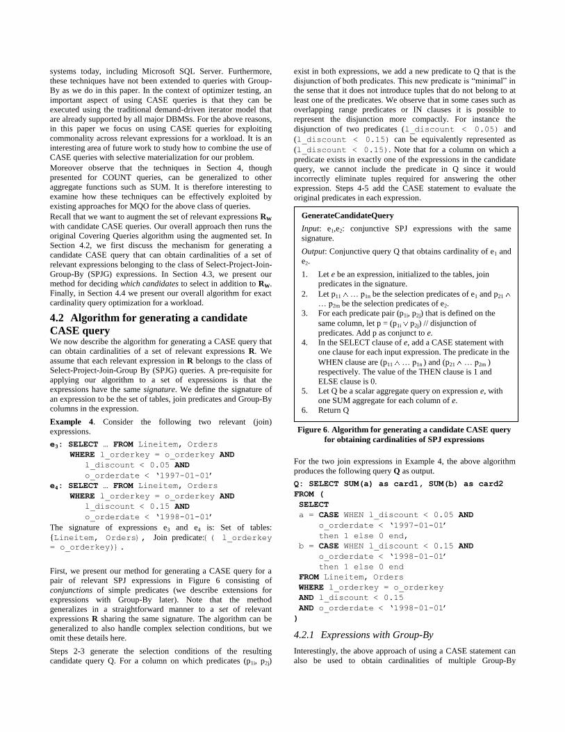
4.2 Algorithm for generating a candidate

CASE query We now describe the algorithm for generating a CASE query that

can obtain cardinalities of a set of relevant expressions R. We

assume that each relevant expression in R belongs to the class of

Select-Project-Join-Group By (SPJG) queries. A pre-requisite for

applying our algorithm to a set of expressions is that the

expressions have the same signature. We define the signature of

an expression to be the set of tables, join predicates and Group-By

columns in the expression.

Example 4. Consider the following two relevant (join)

expressions.

e3: SELECT … FROM Lineitem, Orders

WHERE l_orderkey = o_orderkey AND

l_discount < 0.05 AND

o_orderdate < ‘1997-01-01’

e4: SELECT … FROM Lineitem, Orders

WHERE l_orderkey = o_orderkey AND

l_discount < 0.15 AND

o_orderdate < ‘1998-01-01’

The signature of expressions e3 and e4 is: Set of tables:

{Lineitem, Orders}, Join predicate:{( l_orderkey = o_orderkey)}.

First, we present our method for generating a CASE query for a

pair of relevant SPJ expressions in Figure 6 consisting of

conjunctions of simple predicates (we describe extensions for

expressions with Group-By later). Note that the method

generalizes in a straightforward manner to a set of relevant

expressions R sharing the same signature. The algorithm can be

generalized to also handle complex selection conditions, but we

omit these details here.

Steps 2-3 generate the selection conditions of the resulting

candidate query Q. For a column on which predicates (p1i, p2j)

exist in both expressions, we add a new predicate to Q that is the

disjunction of both predicates. This new predicate is “minimal” in

the sense that it does not introduce tuples that do not belong to at

least one of the predicates. We observe that in some cases such as

overlapping range predicates or IN clauses it is possible to

represent the disjunction more compactly. For instance the

disjunction of two predicates (l_discount < 0.05) and

(l_discount < 0.15) can be equivalently represented as

(l_discount < 0.15). Note that for a column on which a

predicate exists in exactly one of the expressions in the candidate

query, we cannot include the predicate in Q since it would

incorrectly eliminate tuples required for answering the other

expression. Steps 4-5 add the CASE statement to evaluate the

original predicates in each expression.

For the two join expressions in Example 4, the above algorithm

produces the following query Q as output.

Q: SELECT SUM(a) as card1, SUM(b) as card2

FROM (

SELECT

a = CASE WHEN l_discount < 0.05 AND

o_orderdate < ‘1997-01-01’

then 1 else 0 end,

b = CASE WHEN l_discount < 0.15 AND

o_orderdate < ‘1998-01-01’

then 1 else 0 end

FROM Lineitem, Orders

WHERE l_orderkey = o_orderkey

AND l_discount < 0.15

AND o_orderdate < ‘1998-01-01’

)

4.2.1 Expressions with Group-By

Interestingly, the above approach of using a CASE statement can

also be used to obtain cardinalities of multiple Group-By

GenerateCandidateQuery

Input: e1,e2: conjunctive SPJ expressions with the same

signature.

Output: Conjunctive query Q that obtains cardinality of e1 and

e2.

1. Let e be an expression, initialized to the tables, join

predicates in the signature.

2. Let p11 … p1n be the selection predicates of e1 and p21

… p2m be the selection predicates of e2.

3. For each predicate pair (p1i, p2j) that is defined on the

same column, let p = (p1i p2j) // disjunction of

predicates. Add p as conjunct to e.

4. In the SELECT clause of e, add a CASE statement with

one clause for each input expression. The predicate in the

WHEN clause are (p11 … p1n ) and (p21 … p2m )

respectively. The value of the THEN clause is 1 and

ELSE clause is 0.

5. Let Q be a scalar aggregate query on expression e, with

one SUM aggregate for each column of e.

6. Return Q

Figure 6. Algorithm for generating a candidate CASE query

for obtaining cardinalities of SPJ expressions

expressions. We first give an example to illustrate this, and then

describe the necessary extensions to the algorithm of Figure 6.

Example 5. Consider the following two relevant SPJG

expressions. Observe that both expressions have the same

signature, i.e. set of tables, join predicates and Group-By columns.

e1: SELECT o_orderpriority FROM Orders

WHERE o_orderdate between

‘1998-09-01’ and ‘1999-01-01’

GROUP BY o_orderpriority

e2: SELECT o_orderpriority FROM Orders

WHERE o_orderdate between

‘1996-01-01’ and ‘1998-01-01’

GROUP BY o_orderpriority

We can obtain cardinalities of both e1 and e2 using the query Q

below.

Q: SELECT SUM(a1) as card1, SUM(b1)as card2

FROM (

SELECT

a1 = CASE when (q1 > 0)then 1 else 0 end,

b1 = CASE when (q2 > 0)then 1 else 0 end

FROM (

SELECT o_orderpriority,

SUM(a) as q1,SUM(b) as q2

FROM (

SELECT o_orderpriority,

a = CASE when (o_orderdate between

'1998-09-01' and ‘1999-01-01’) then 1

else 0 end,

b = CASE when (o_orderdate between

'1996-01-01' and '1998-01-01') then 1

else 0 end

FROM (

SELECT o_orderpriority, o_orderdate

FROM Orders

WHERE o_orderdate between

'1996-01-01' and '1999-01-01'

GROUP BY o_orderpriority, o_orderdate

))

GROUP BY o_orderpriority

)

)

From the structure of query Q, we note a couple of points. First,

the innermost SELECT statement needs to generate a more

“finer” grouping (by including the selection columns in the

GROUP BY clause) than either e1 or e2. This is because the

selection column(s) are required in the CASE clause. Second,

unlike the algorithm for SPJ expressions, for SPJG expressions we

require two nested CASE queries. The inner CASE query

computes a row for each group that is in the result of either e1 or

e2 (or both). However, recollect that we need to find the number of

groups in e1 and e2 respectively. Thus, the outer CASE query is

necessary to ensure that we do not incorrectly count a group that

occurs exclusively in e1 as part of e2 (or vice versa). Despite the

fact that Q is more complex than either e1 or e2, it can potentially

be more efficient than the combined cost of executing both e1 and

e2. For example, if both e1 and e2 scan the (large) Orders table,

the Q could be more efficient since it would need to scan

Orders only once.

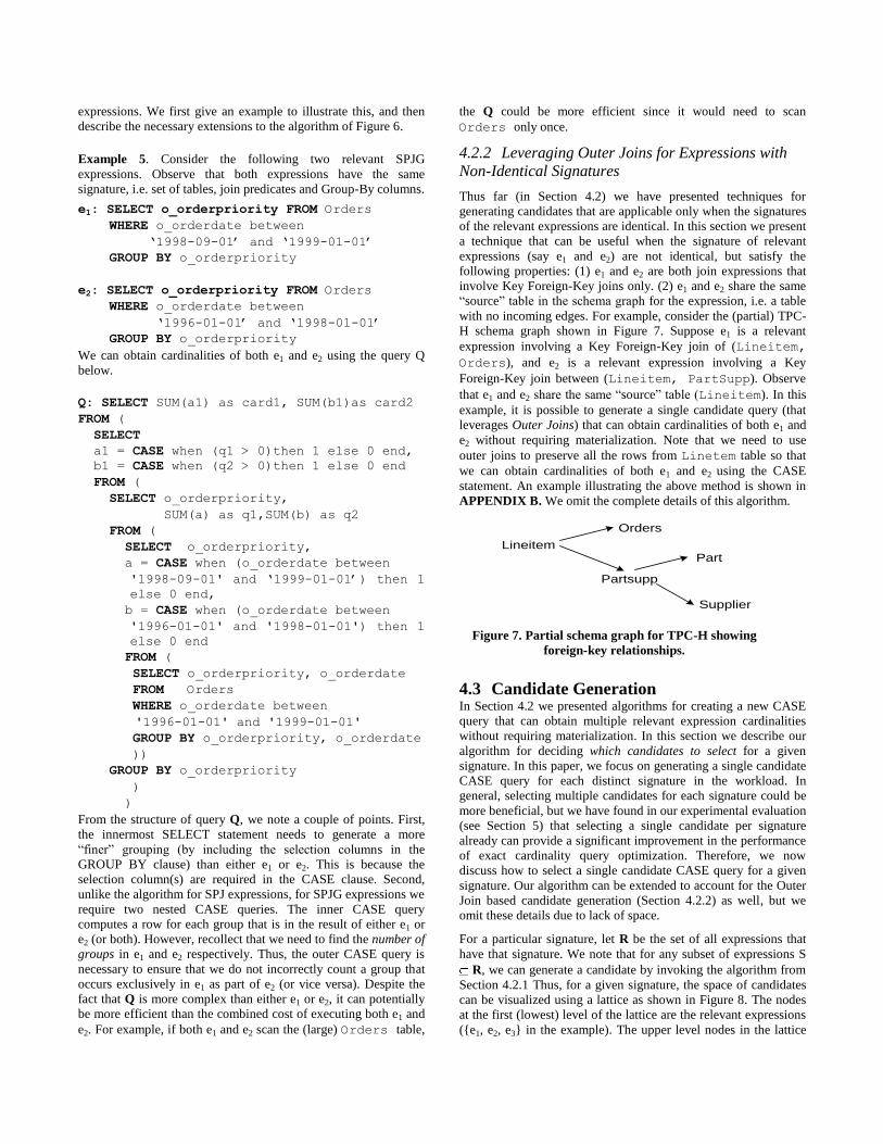
4.2.2 Leveraging Outer Joins for Expressions with

Non-Identical Signatures

Thus far (in Section 4.2) we have presented techniques for

generating candidates that are applicable only when the signatures

of the relevant expressions are identical. In this section we present

a technique that can be useful when the signature of relevant

expressions (say e1 and e2) are not identical, but satisfy the

following properties: (1) e1 and e2 are both join expressions that

involve Key Foreign-Key joins only. (2) e1 and e2 share the same

“source” table in the schema graph for the expression, i.e. a table

with no incoming edges. For example, consider the (partial) TPC-

H schema graph shown in Figure 7. Suppose e1 is a relevant

expression involving a Key Foreign-Key join of (Lineitem,

Orders), and e2 is a relevant expression involving a Key

Foreign-Key join between (Lineitem, PartSupp). Observe

that e1 and e2 share the same “source” table (Lineitem). In this

example, it is possible to generate a single candidate query (that

leverages Outer Joins) that can obtain cardinalities of both e1 and

e2 without requiring materialization. Note that we need to use

outer joins to preserve all the rows from Linetem table so that

we can obtain cardinalities of both e1 and e2 using the CASE

statement. An example illustrating the above method is shown in

APPENDIX B. We omit the complete details of this algorithm.

LineitemPart

Partsupp

Orders

Supplier

4.3 Candidate Generation In Section 4.2 we presented algorithms for creating a new CASE

query that can obtain multiple relevant expression cardinalities

without requiring materialization. In this section we describe our

algorithm for deciding which candidates to select for a given

signature. In this paper, we focus on generating a single candidate

CASE query for each distinct signature in the workload. In

general, selecting multiple candidates for each signature could be

more beneficial, but we have found in our experimental evaluation

(see Section 5) that selecting a single candidate per signature

already can provide a significant improvement in the performance

of exact cardinality query optimization. Therefore, we now

discuss how to select a single candidate CASE query for a given

signature. Our algorithm can be extended to account for the Outer

Join based candidate generation (Section 4.2.2) as well, but we

omit these details due to lack of space.

For a particular signature, let R be the set of all expressions that

have that signature. We note that for any subset of expressions S

R, we can generate a candidate by invoking the algorithm from

Section 4.2.1 Thus, for a given signature, the space of candidates

can be visualized using a lattice as shown in Figure 8. The nodes

at the first (lowest) level of the lattice are the relevant expressions

({e1, e2, e3} in the example). The upper level nodes in the lattice

Figure 7. Partial schema graph for TPC-H showing

foreign-key relationships.

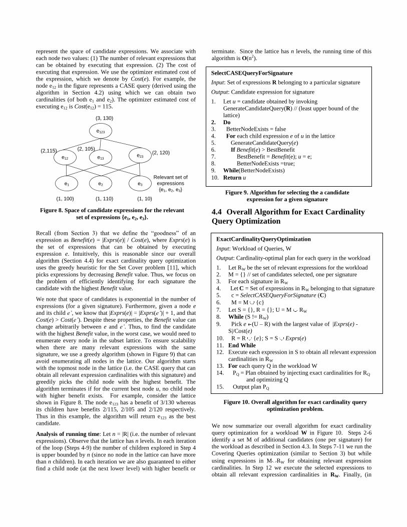
represent the space of candidate expressions. We associate with

each node two values: (1) The number of relevant expressions that

can be obtained by executing that expression. (2) The cost of

executing that expression. We use the optimizer estimated cost of

the expression, which we denote by Cost(e). For example, the

node e12 in the figure represents a CASE query (derived using the

algorithm in Section 4.2) using which we can obtain two

cardinalities (of both e1 and e2). The optimizer estimated cost of

executing e12 is Cost(e12) = 115.

e123

e12 e13e23

e1 e2 e3

Relevant set of

expressions

{e1, e2, e3}

(1, 100) (1, 110) (1, 10)

(2,115) (2, 105)(2, 120)

(3, 130)

Recall (from Section 3) that we define the “goodness” of an

expression as Benefit(e) = |Exprs(e)| / Cost(e), where Exprs(e) is

the set of expressions that can be obtained by executing

expression e. Intuitively, this is reasonable since our overall

algorithm (Section 4.4) for exact cardinality query optimization

uses the greedy heuristic for the Set Cover problem [11], which

picks expressions by decreasing Benefit value. Thus, we focus on

the problem of efficiently identifying for each signature the

candidate with the highest Benefit value.

We note that space of candidates is exponential in the number of

expressions (for a given signature). Furthermore, given a node e

and its child e’, we know that |Exprs(e)| = |Exprs(e’)| + 1, and that

Cost(e) > Cost(e’). Despite these properties, the Benefit value can

change arbitrarily between e and e’. Thus, to find the candidate

with the highest Benefit value, in the worst case, we would need to

enumerate every node in the subset lattice. To ensure scalability

when there are many relevant expressions with the same

signature, we use a greedy algorithm (shown in Figure 9) that can

avoid enumerating all nodes in the lattice. Our algorithm starts

with the topmost node in the lattice (i.e. the CASE query that can

obtain all relevant expression cardinalities with this signature) and

greedily picks the child node with the highest benefit. The

algorithm terminates if for the current best node u, no child node

with higher benefit exists. For example, consider the lattice

shown in Figure 8. The node e123 has a benefit of 3/130 whereas

its children have benefits 2/115, 2/105 and 2/120 respectively.

Thus in this example, the algorithm will return e123 as the best

candidate.

Analysis of running time: Let n = |R| (i.e. the number of relevant

expressions). Observe that the lattice has n levels. In each iteration

of the loop (Steps 4-9) the number of children explored in Step 4

is upper bounded by n (since no node in the lattice can have more

than n children). In each iteration we are also guaranteed to either

find a child node (at the next lower level) with higher benefit or

terminate. Since the lattice has n levels, the running time of this

algorithm is O(n2).

4.4 Overall Algorithm for Exact Cardinality

Query Optimization

.

We now summarize our overall algorithm for exact cardinality

query optimization for a workload W in Figure 10. Steps 2-6

identify a set M of additional candidates (one per signature) for

the workload as described in Section 4.3. In Steps 7-11 we run the

Covering Queries optimization (similar to Section 3) but while

using expressions in M RW for obtaining relevant expression

cardinalities. In Step 12 we execute the selected expressions to

obtain all relevant expression cardinalities in RW. Finally, (in

Figure 10. Overall algorithm for exact cardinality query

optimization problem.

ExactCardinalityQueryOptimization

Input: Workload of Queries, W

Output: Cardinality-optimal plan for each query in the workload

1. Let RW be the set of relevant expressions for the workload

2. M = {} // set of candidates selected, one per signature

3. For each signature in RW

4. Let C = Set of expressions in RW belonging to that signature

5. c = SelectCASEQueryForSignature (C)

6. M = M {c}

7. Let S = {}, R = {}; U = M RW

8. While (S != RW)

9. Pick e (U – R) with the largest value of |Exprs(e) -

S|/Cost(e)

10. R = R {e}; S = S Exprs(e)

11. End While

12. Execute each expression in S to obtain all relevant expression

cardinalities in RW

13. For each query Q in the workload W

14. PQ = Plan obtained by injecting exact cardinalities for RQ

and optimizing Q

15. Output plan PQ

Figure 9. Algorithm for selecting the a candidate

expression for a given signature

Figure 8. Space of candidate expressions for the relevant

set of expressions {e1, e2, e3}.

SelectCASEQueryForSignature

Input: Set of expressions R belonging to a particular signature

Output: Candidate expression for signature

1. Let u = candidate obtained by invoking

GenerateCandidateQuery(R) // (least upper bound of the

lattice)

2. Do

3. BetterNodeExists = false

4. For each child expression e of u in the lattice

5. GenerateCandidateQuery(e)

6. If Benefit(e) > BestBenefit

7. BestBenefit = Benefit(e); u = e;

8. BetterNodeExists =true;

9. While(BetterNodeExists)

10. Return u

Steps 13-15) for each query in the workload, we inject the exact

cardinalities for all relevant expressions for that query and obtain

the cardinality-optimal plan for that query. As we demonstrate in

our experiments (Section 5) candidate generation can significantly

improve the effectiveness of the Covering Queries optimization.

5. IMPLEMENTATION AND

EXPERIMENTS Implementation: We have implemented a prototype of Exact

Cardinality Query Optimization on Microsoft SQL Server. The

extensions were as described in the architecture outlined in Figure

2. We implemented the Covering Queries Optimization (Section

3) as well as the Candidate Generation techniques presented in

Section 4. Our experiments were run on a machine with an AMD

Opteron processor (2.40 GHz, 8 GB RAM).

Databases and Queries: We use the TPC-H benchmark [22]

(both the 1GB version and the 10GB version). The original data

generator [22] does not introduce any skew in the data. Thus, in

addition to the original benchmark database, we also use a data

generator that introduces a skewed distribution (a Zipfian

distribution with a skew factor of Z = 1) for each column

independently in a relation [6]. We use a workload consisting of

all queries having two or more joins.

The goals of our experiments are:

Evaluate the effectiveness of the Covering Queries algorithm

(Section 3) for the case of a single query compared to the

baseline strategy of executing each relevant expression.

For the case of a workload, evaluate the importance of the

Candidate Generation techniques (Section 4) for reducing the

execution time compared to the approach of using Covering

Queries for one query at a time.

Show some examples of analytics for optimizer testing that

are enabled once exact cardinalities are available.

5.1 Effectiveness of Techniques for Single

Query As mentioned above we use a workload of queries from the TPC-

H benchmark [22]. The number of relevant expressions (|RQ|) for

queries varied from 6 (for a few of the simpler queries) to 30. For

the 1GB version of the benchmark, for most queries, the time

taken to obtain all cardinalities (by executing their corresponding

expressions) is in the order of a few minutes. The corresponding

number for the 10GB version varies from 10s of minutes to over

an hour for some queries.

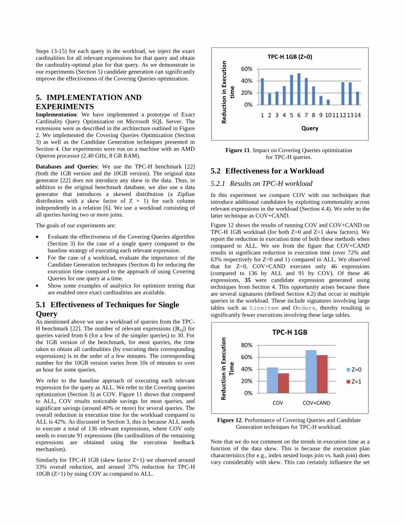
We refer to the baseline approach of executing each relevant

expression for the query as ALL. We refer to the Covering queries

optimization (Section 3) as COV. Figure 11 shows that compared

to ALL, COV results noticeable savings for most queries, and

significant savings (around 40% or more) for several queries. The

overall reduction in execution time for the workload compared to

ALL is 42%. As discussed in Section 3, this is because ALL needs

to execute a total of 136 relevant expressions, where COV only

needs to execute 91 expressions (the cardinalities of the remaining

expressions are obtained using the execution feedback

mechanism).

Similarly for TPC-H 1GB (skew factor Z=1) we observed around

33% overall reduction, and around 37% reduction for TPC-H

10GB (Z=1) by using COV as compared to ALL.

5.2 Effectiveness for a Workload

5.2.1 Results on TPC-H workload

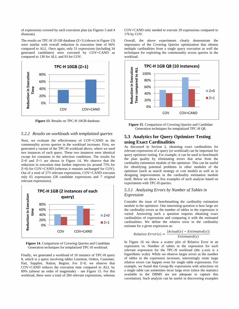
In this experiment we compare COV with our techniques that

introduce additional candidates by exploiting commonality across

relevant expressions in the workload (Section 4.4). We refer to the

latter technique as COV+CAND.

Figure 12 shows the results of running COV and COV+CAND on

TPC-H 1GB workload (for both Z=0 and Z=1 skew factors). We

report the reduction in execution time of both these methods when

compared to ALL. We see from the figure that COV+CAND

results in significant reduction in execution time (over 72% and

63% respectively for Z=0 and 1) compared to ALL. We observed

that for Z=0, COV+CAND executes only 46 expressions

(compared to 136 by ALL and 91 by COV). Of these 46

expressions, 35 were candidate expression generated using

techniques from Section 4. This opportunity arises because there

are several signatures (defined Section 4.2) that occur in multiple

queries in the workload. These include signatures involving large

tables such as Lineitem and Orders, thereby resulting in

significantly fewer executions involving these large tables.

Note that we do not comment on the trends in execution time as a

function of the data skew. This is because the execution plan

characteristics (for e.g., index nested loops join vs. hash join) does

vary considerably with skew. This can certainly influence the set

0%

20%

40%

60%

1 2 3 4 5 6 7 8 9 1011121314

Re

du

ctio

n in

Exe

cuti

on

ti

me

Query

TPC-H 1GB (Z=0)

0%

20%

40%

60%

80%

COV COV+CAND

Re

du

ctio

n in

Exe

cuti

on

Ti

me

TPC-H 1GB

Z=0

Z=1

Figure 11. Impact on Covering Queries optimization

for TPC-H queries.

Figure 12. Performance of Covering Queries and Candidate

Generation techniques for TPC-H workload.

of expressions covered by each execution plan (as Figures 3 and 4

illustrate).

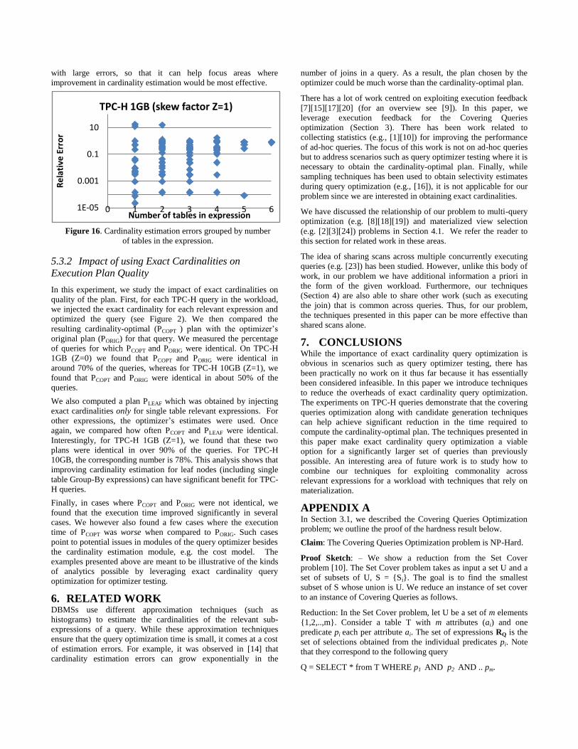
The results on TPC-H 10 GB database (Z=1) (shown in Figure 13)

were similar with overall reduction in execution time of 66%

compared to ALL. Once again, only 51 expressions (including 34

generated candidates) were executed by COV+CAND as

compared to 130 for ALL and 93 for COV.

5.2.2 Results on workloads with templatized queries

Next, we evaluate the effectiveness of COV+CAND as the

commonality across queries in the workload increases. First, we

generated a variant of the TPC-H workload above, where we used

two instances of each query. These two instances were identical

except for constants in the selection conditions. The results for

Z=0 and Z=1 are shown in Figure 14. We observe that the

reduction in execution time further improves (to around 75% for

Z=0) for COV+CAND (whereas it remains unchanged for COV).

Out of a total of 273 relevant expressions, COV+CAND executes

only 65 expressions (58 candidate expressions and 7 original

relevant expressions).

Finally, we generated a workload of 10 instance of TPC-H query

8, which is a query involving tables Lineitem, Orders, Customer,

Part, Supplier, Nation, Region. For Z=0, we observe that

COV+CAND reduces the execution time compared to ALL by

89% (almost an order of magnitude) – see Figure 15. For this

workload, there were a total of 284 relevant expressions, whereas

COV+CAND only needed to execute 29 expressions compared to

176 by COV.

Overall, the above experiments clearly demonstrate the

importance of the Covering Queries optimization that obtains

multiple cardinalities from a single query execution as well the

techniques for exploiting the commonality across queries in the

workload.

5.3 Analytics for Query Optimizer Testing

using Exact Cardinalities As discussed in Section 2, obtaining exact cardinalities for

relevant expressions of a query (or workload) can be important for

query optimizer testing. For example, it can be used to benchmark

the plan quality by eliminating errors that arise from the

cardinality estimation module of the optimizer. This can be useful

for identifying potential problems in other modules of the

optimizer (such as search strategy or cost model) as well as in

designing improvements in the cardinality estimation module

itself. Below we show a few examples of such analysis based on

experiments with TPC-H queries.

5.3.1 Analyzing Errors by Number of Tables in

Expression

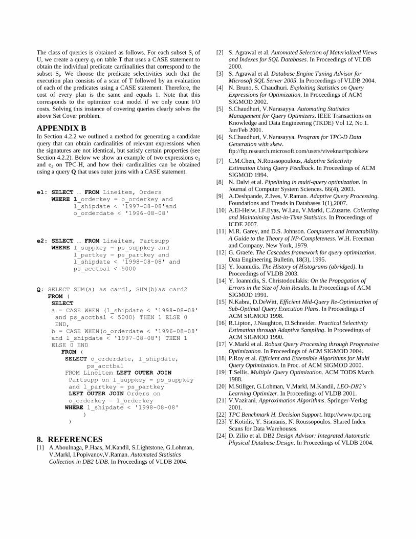
Consider the issue of benchmarking the cardinality estimation

module in the optimizer. One interesting question is how large are

the cardinality errors as the number of tables in the expression is

varied. Answering such a question requires obtaining exact

cardinalities of expressions and comparing it with the estimated

cardinalities. We define the relative error in the cardinality

estimate for a given expression as:

In Figure 16 we show a scatter plot of Relative Error in an

expression vs. Number of tables in the expression for each

relevant expression for the TPC-H workload (the y-axis is a

logarithmic scale). While we observe larger errors as the number

of tables in the expression increases, interestingly some large

relative errors can happen even for single table expressions. For

example, we found that Group-By expressions with selections on

a single table can sometimes incur large error (since the statistics

available in the DBMS are not adequate to capture this

correlation). Such analysis can be useful in discovering examples

0%

20%

40%

60%

80%

COV COV+CANDRe

du

ctio

n in

Exe

cuti

on

Ti

me

TPC-H 10GB (Z=1)

0%

20%

40%

60%

80%

COV COV+CAND

Re

du

ctio

n in

Exe

cuti

on

ti

me

TPC-H 1GB (2 instances of each query)

Z=0

Z=1

0%

20%

40%

60%

80%

100%

COV COV+CAND

Re

du

ctio

n in

Exe

cuti

on

Ti

me

co

mp

are

d t

o A

LL

TPC-H 1GB Q8 (10 instances)

Z=0

Z=1

Figure 14. Comparison of Covering Queries and Candidate

Generation techniques for templatized TPC-H workload.

Figure 15. Comparison of Covering Queries and Candidate

Generation techniques for templatized TPC-H Q8.

Figure 13. Results on TPC-H 10GB database.

with large errors, so that it can help focus areas where

improvement in cardinality estimation would be most effective.

5.3.2 Impact of using Exact Cardinalities on

Execution Plan Quality

In this experiment, we study the impact of exact cardinalities on

quality of the plan. First, for each TPC-H query in the workload,

we injected the exact cardinality for each relevant expression and

optimized the query (see Figure 2). We then compared the

resulting cardinality-optimal (PCOPT ) plan with the optimizer‟s

original plan (PORIG) for that query. We measured the percentage

of queries for which PCOPT and PORIG were identical. On TPC-H

1GB (Z=0) we found that PCOPT and PORIG were identical in

around 70% of the queries, whereas for TPC-H 10GB (Z=1), we

found that PCOPT and PORIG were identical in about 50% of the

queries.

We also computed a plan PLEAF which was obtained by injecting

exact cardinalities only for single table relevant expressions. For

other expressions, the optimizer‟s estimates were used. Once

again, we compared how often PCOPT and PLEAF were identical.

Interestingly, for TPC-H 1GB (Z=1), we found that these two

plans were identical in over 90% of the queries. For TPC-H

10GB, the corresponding number is 78%. This analysis shows that

improving cardinality estimation for leaf nodes (including single

table Group-By expressions) can have significant benefit for TPC-

H queries.

Finally, in cases where PCOPT and PORIG were not identical, we

found that the execution time improved significantly in several

cases. We however also found a few cases where the execution

time of PCOPT was worse when compared to PORIG. Such cases

point to potential issues in modules of the query optimizer besides

the cardinality estimation module, e.g. the cost model. The

examples presented above are meant to be illustrative of the kinds

of analytics possible by leveraging exact cardinality query

optimization for optimizer testing.

6. RELATED WORK DBMSs use different approximation techniques (such as

histograms) to estimate the cardinalities of the relevant sub-

expressions of a query. While these approximation techniques

ensure that the query optimization time is small, it comes at a cost

of estimation errors. For example, it was observed in [14] that

cardinality estimation errors can grow exponentially in the

number of joins in a query. As a result, the plan chosen by the

optimizer could be much worse than the cardinality-optimal plan.

There has a lot of work centred on exploiting execution feedback

[7][15][17][20] (for an overview see [9]). In this paper, we

leverage execution feedback for the Covering Queries

optimization (Section 3). There has been work related to

collecting statistics (e.g., [1][10]) for improving the performance

of ad-hoc queries. The focus of this work is not on ad-hoc queries

but to address scenarios such as query optimizer testing where it is

necessary to obtain the cardinality-optimal plan. Finally, while

sampling techniques has been used to obtain selectivity estimates

during query optimization (e.g., [16]), it is not applicable for our

problem since we are interested in obtaining exact cardinalities.

We have discussed the relationship of our problem to multi-query

optimization (e.g. [8][18][19]) and materialized view selection

(e.g. [2][3][24]) problems in Section 4.1. We refer the reader to

this section for related work in these areas.

The idea of sharing scans across multiple concurrently executing

queries (e.g. [23]) has been studied. However, unlike this body of

work, in our problem we have additional information a priori in

the form of the given workload. Furthermore, our techniques

(Section 4) are also able to share other work (such as executing

the join) that is common across queries. Thus, for our problem,

the techniques presented in this paper can be more effective than

shared scans alone.

7. CONCLUSIONS While the importance of exact cardinality query optimization is

obvious in scenarios such as query optimizer testing, there has

been practically no work on it thus far because it has essentially

been considered infeasible. In this paper we introduce techniques

to reduce the overheads of exact cardinality query optimization.

The experiments on TPC-H queries demonstrate that the covering

queries optimization along with candidate generation techniques

can help achieve significant reduction in the time required to

compute the cardinality-optimal plan. The techniques presented in

this paper make exact cardinality query optimization a viable

option for a significantly larger set of queries than previously

possible. An interesting area of future work is to study how to

combine our techniques for exploiting commonality across

relevant expressions for a workload with techniques that rely on

materialization.

APPENDIX A In Section 3.1, we described the Covering Queries Optimization

problem; we outline the proof of the hardness result below.

Claim: The Covering Queries Optimization problem is NP-Hard.

Proof Sketch: – We show a reduction from the Set Cover

problem [10]. The Set Cover problem takes as input a set U and a

set of subsets of U, S = {Si}. The goal is to find the smallest

subset of S whose union is U. We reduce an instance of set cover

to an instance of Covering Queries as follows.

Reduction: In the Set Cover problem, let U be a set of m elements

{1,2,..,m}. Consider a table T with m attributes (ai) and one

predicate pi each per attribute ai. The set of expressions RQ is the

set of selections obtained from the individual predicates pi. Note

that they correspond to the following query

Q = SELECT * from T WHERE p1 AND p2 AND .. pm.

1E-05

0.001

0.1

10

0 1 2 3 4 5 6

Re

lati

ve E

rro

r

Number of tables in expression

TPC-H 1GB (skew factor Z=1)

Figure 16. Cardinality estimation errors grouped by number

of tables in the expression.

The class of queries is obtained as follows. For each subset Si of

U, we create a query qi on table T that uses a CASE statement to

obtain the individual predicate cardinalities that correspond to the

subset Si. We choose the predicate selectivities such that the

execution plan consists of a scan of T followed by an evaluation

of each of the predicates using a CASE statement. Therefore, the

cost of every plan is the same and equals 1. Note that this

corresponds to the optimizer cost model if we only count I/O

costs. Solving this instance of covering queries clearly solves the

above Set Cover problem.

APPENDIX B In Section 4.2.2 we outlined a method for generating a candidate

query that can obtain cardinalities of relevant expressions when

the signatures are not identical, but satisfy certain properties (see

Section 4.2.2). Below we show an example of two expressions e1

and e2 on TPC-H, and how their cardinalities can be obtained

using a query Q that uses outer joins with a CASE statement.

e1: SELECT … FROM Lineitem, Orders

WHERE l_orderkey = o_orderkey and

l_shipdate < '1997-08-08'and

o_orderdate < '1996-08-08'

e2: SELECT … FROM Lineitem, Partsupp

WHERE l_suppkey = ps_suppkey and

l_partkey = ps_partkey and

l_shipdate < '1998-08-08' and

ps_acctbal < 5000

Q: SELECT SUM(a) as card1, SUM(b)as card2

FROM (

SELECT

a = CASE WHEN (l_shipdate < '1998-08-08'

and ps_acctbal < 5000) THEN 1 ELSE 0

END,

b = CASE WHEN(o_orderdate < '1996-08-08'

and l_shipdate < '1997-08-08') THEN 1

ELSE 0 END

FROM (

SELECT o_orderdate, l_shipdate,

ps_acctbal

FROM Lineitem LEFT OUTER JOIN

Partsupp on l_suppkey = ps_suppkey

and l_partkey = ps_partkey

LEFT OUTER JOIN Orders on

o_orderkey = l_orderkey

WHERE l_shipdate < '1998-08-08'

)

)

8. REFERENCES [1] A.Aboulnaga, P.Haas, M.Kandil, S.Lightstone, G.Lohman,

V.Markl, I.Popivanov,V.Raman. Automated Statistics

Collection in DB2 UDB. In Proceedings of VLDB 2004.

[2] S. Agrawal et al. Automated Selection of Materialized Views

and Indexes for SQL Databases. In Proceedings of VLDB

2000.

[3] S. Agrawal et al. Database Engine Tuning Advisor for

Microsoft SQL Server 2005. In Proceedings of VLDB 2004.

[4] N. Bruno, S. Chaudhuri. Exploiting Statistics on Query

Expressions for Optimization. In Proceedings of ACM

SIGMOD 2002.

[5] S.Chaudhuri, V.Narasayya. Automating Statistics

Management for Query Optimizers. IEEE Transactions on

Knowledge and Data Engineering (TKDE) Vol 12, No 1.

Jan/Feb 2001.

[6] S.Chaudhuri, V.Narasayya. Program for TPC-D Data

Generation with skew.

ftp://ftp.research.microsoft.com/users/viveknar/tpcdskew

[7] C.M.Chen, N.Roussopoulous, Adaptive Selectivity

Estimation Using Query Feedback. In Proceedings of ACM

SIGMOD 1994.

[8] N. Dalvi et al. Pipelining in multi-query optimization. In

Journal of Computer System Sciences. 66(4), 2003.

[9] A.Deshpande, Z.Ives, V.Raman. Adaptive Query Processing.

Foundations and Trends in Databases 1(1),2007.

[10] A.El-Helw, I.F.Ilyas, W.Lau, V.Markl, C.Zuzarte. Collecting

and Maintaining Just-in-Time Statistics. In Proceedings of

ICDE 2007.

[11] M.R. Garey, and D.S. Johnson. Computers and Intractability.

A Guide to the Theory of NP-Completeness. W.H. Freeman

and Company, New York, 1979.

[12] G. Graefe. The Cascades framework for query optimization.

Data Engineering Bulletin, 18(3), 1995.

[13] Y. Ioannidis. The History of Histograms (abridged). In

Proceedings of VLDB 2003.

[14] Y. Ioannidis, S. Christodoulakis: On the Propagation of

Errors in the Size of Join Results. In Proceedings of ACM

SIGMOD 1991.

[15] N.Kabra, D.DeWitt, Efficient Mid-Query Re-Optimization of

Sub-Optimal Query Execution Plans. In Proceedings of

ACM SIGMOD 1998.

[16] R.Lipton, J.Naughton, D.Schneider. Practical Selectivity

Estimation through Adaptive Sampling. In Proceedings of

ACM SIGMOD 1990.

[17] V.Markl et al. Robust Query Processing through Progressive

Optimization. In Proceedings of ACM SIGMOD 2004.

[18] P.Roy et al. Efficient and Extensible Algorithms for Multi

Query Optimization. In Proc. of ACM SIGMOD 2000.

[19] T.Sellis. Multiple Query Optimization. ACM TODS March

1988.

[20] M.Stillger, G.Lohman, V.Markl, M.Kandil, LEO-DB2’s

Learning Optimizer. In Proceedings of VLDB 2001.

[21] V.Vazirani. Approximation Algorithms. Springer-Verlag

2001.

[22] TPC Benchmark H. Decision Support. http://www.tpc.org

[23] Y.Kotidis, Y. Sismanis, N. Roussopoulos. Shared Index

Scans for Data Warehouses.

[24] D. Zilio et al. DB2 Design Advisor: Integrated Automatic

Physical Database Design. In Proceedings of VLDB 2004.