evaluation(u) university unlsiidwst/l-hm hhf0hh10hl- … · station (wes) undertook the design and...
TRANSCRIPT

91tf 4N FAST TRIAXIAL SNEAR DEVICE EVALUATION(U) UNIVERSITY OF UEJI~h NA CECSI RRL ACENTRAL FLORIDA ORLANDO DEPT OF CIVIL ENGINEERING AND
ENVIROW ~ ~ ~ /f I/SL SCECSN ARLLJNOUNLSIIDWST/l-hm hhF0hh10hl-~l-ENOhMONEu
Emhhhmhhhhhu
-ILI, -
L6L.~ .-O .
111IL25 .4-.
A."
I.'Nfl I' ,jj j J

TECHNICAL REPORT SL-88-2
FAST TRIAXIAL SHEAR DEVICE EAUTOof EVALUATION
by
o William F. Carroll
0Department of Civil Engineeringand Environmental SciencesUniversity of Central Florida
Orlando, Florida 32816
0,T
i ill :LECTE h
c.YD
January 1988Final Report
Approved For Public Release Distribution Unlimited
*%
40
S',,,,,DEPARTMENT OF THE ARMYUS Army Corps of EngineersWashington, DC 20314-1000 S
C,,, ij,, Project No. 4A161102AT22, Task BO, Work Unit 005
Moilorret b, Structures Laboratory
LABORATORY US Army Engineer Waterways Experiment StationPO Box 631, Vicksburg, Mississippi 39180-06311 88 2 29 U54
UnclassifiedSECURITY CLASSIFICATION OF THIS PAGEF
REPORT DOCUMENTATION PAGE OB10074. 1
la REPORT SECURITY CLASSIFICATION lb RESTRICTIVE MARIKIN,.SUnclassified2a. SECURITY CLASSIFICATION AUTHORITY J DSTRIOBUTION/AVALABILITY OF REPORT
Approved for public release; distribution2b. DECLASSIFICATION / DOWNGRADING SCHEDULE unlimited.
4. PERFORMING ORGANIZATION REPORT NUMBER(S) S MONITORING ORGANIZATION REPORT NUMBER(S)
Technical Report SL-88-2
6a. NAME OF PERFORMING ORGANIZATION 6b OFFICE SYMBOL 7a NAME OF MONITORING ORGANIZATION
University of Central Florida (Ifcaj USAEWES
6c. ADDRESS (City, State. and ZIP Code) 7b ADDRESS(ty, State. and ZIP Code)
Orlando, FL 32816 Po Box 631Vicksburg, MS 39180-0631
8.. NAME OF FUNDING/SPONSORING -Bb OFFICE SYMBOL 9 PROCUREMENT INSTRUMENT IDENTIFICATION NUMBERORGANIZATION (If applicable)
US Army Corps of EngineersSc. ADDRESS (City, State, and ZIP Code) 10 SOURCE OF FUNDING NUMBERS20 Massachusetts Ave., N.W. PROGRAM PROJECT ASK WORK UNIT
ELEMENT NO NO NO ACCESSION NOWashington, DC 20314-1000 4A61102AT22 BO 005"
11 TITLE (Include Security Classification)
Fast Triaxial Shear Device Evaluation
12 PERSONAL AUTHOR(S)Carroll, William F.13a TYPE OF REPORT 13b TIME COVERED 14 DATE OF REPORT (Year. Month, Day) 15 PAGE COUNTFinal report FROM _ TO January 1988 9916. SUPPLEMENTARY NOTATIONAvailable from National Technical Information Service, 5285 Port Royal Road,Springfield, VA 22161.17. COSATI CODES 18. SUBJECT TERMS (Continue on reverse if necessary and identify by block number)
FIELD GROUP SUB-GROUP Dynamic soil properties Shear strengthLoading rate effects Stress-strainOne-dimensional wave analyses Triaxial shear tests
19 ABSTRACT (Continue on reverse if necessary and identify by block number)
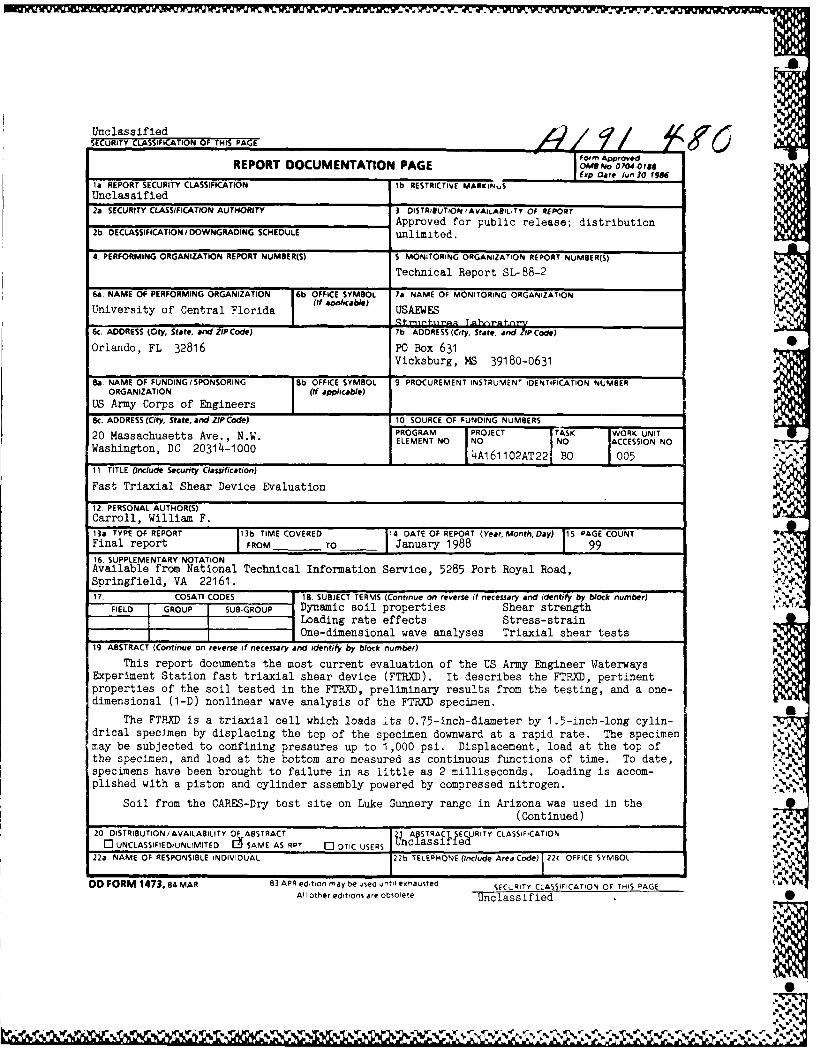
This report documents the most current evaluation of the US Army Engineer WaterwaysExperiment Station fast triaxial shear device (FTRXD). It describes the FTRXD, pertinentproperties of the soil tested in the FTRXD, preliminary results from the testing, and a one-dimensional (1-D) nonlinear wave analysis of the FTRXD specimen.
The FTRXD is a triaxial cell which loads its 0.75-inch-diameter by 1.5-inch-long cylin-drical specimen by displacing the top of the specimen downward at a rapid rate. The specimenmay be subjected to confining pressures up to 1 ,000 psi. Displacement, load at the top ofthe specimen, and load at the bottom are measured as continuous functions of time. To date,specimens have been brought to failure in as little as 2 milliseconds. Loading is accom-plished with a piston and cylinder assembly powered by compressed nitrogen.
Soil from the CARES-Dry test site on Luke Gunnery range in Arizona was used in the(Continued)
20 DISTRIBUTION/ AVAILABILITY OF ABSTRACT AI STRACTIECRTY CLASSIFICATIONC UNCLASSIFIEDIUNLIMITED ff SAME AS RPT C OTIC USERS Uncassif e
22a NAME OF RESPONSIBLE INDIVIDUAL 22b TELEPHONE (Include Area Code) 22c OFFICE SYMBOL
DD FORM 1473, 84 MAR 83 APR edition may be used untI eiausted SECLRITY CLASSIFICATION OF THIS PAGE 1011
All other editions are obsolete Unclassified 0
I o15-~~~- ,r 5. %-- W~ ~Vr , ,.. (~
. ~ ~ . S.
M.I M I .-. . .~fF ....l V
UnclassifiedSWECURITY CLASSIFICATION OF THIS PAGE_
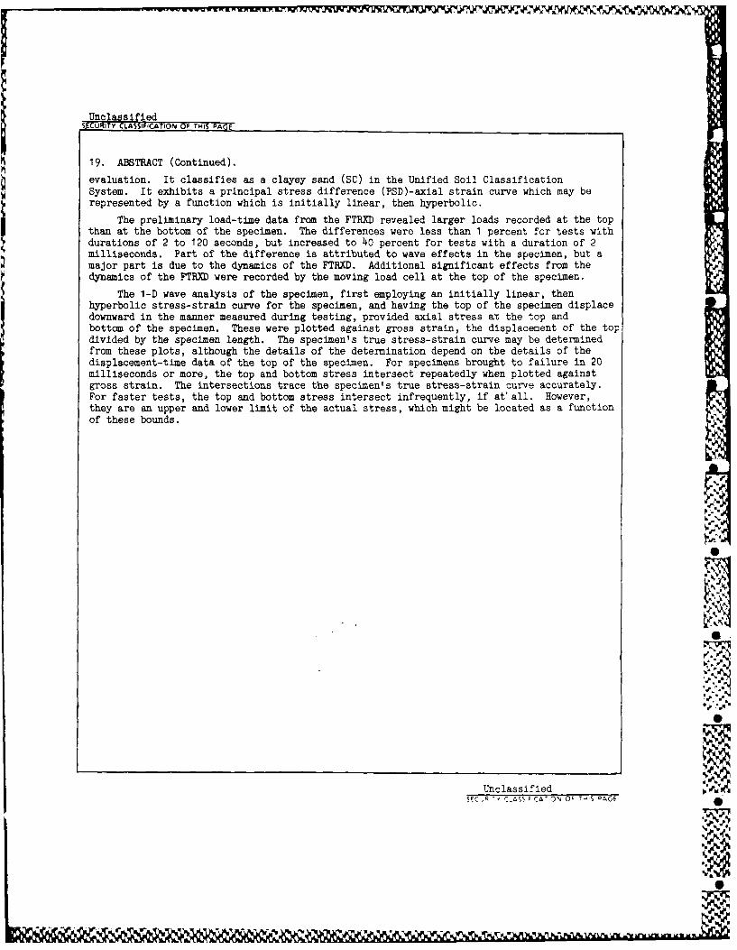
19. ABSTRACT (Continued).
evaluation. It classifies as a clayey sand (SC) in the Unified Soil ClassificationSystem. It exhibits a principal stress difference (PSD)-axial strain curve which may berepresented by a function which is initially linear, then hyperbolic.
The preliminary load-time data from the FTRXD revealed larger loads recorded at the topthan at the bottom of the specimen. The differences were less than I percent for tests withdurations of 2 to 120 seconds, but increased to 40 percent for tests with a duration of 2milliseconds. Part of the difference is attributed to wave effects in the specimen, but amajor part is due to the dynamics of the FTRXD. Additional significant effects from thedynamics of the FTRXD were recorded by the moving load cell at the top of the specimen.
The 1-D wave analysis of the specimen, first employing an initially linear, thenhyperbolic stress-strain curve for the specimen, and having the top of the specimen displacedownward in the manner measured during testing, provided axial stress at the top andbottom of the specimen. These were plotted against gross strain, the displacement of the topdivided by the specimen length. The specimen's true stress-strain curve may be determinedfrom these plots, although the details of the determination depend on the details of thedisplacement-time data of the top of the specimen. For specimens brought to failure in 20milliseconds or more, the top and bottom stress intersect repeatedly when plotted againstgross strain. The intersections trace the specimen's true stress-strain curve accurately.For faster tests, the top and bottom stress intersect infrequently, if at' all. However,they are an upper and lower limit of the actual stress, which might be located as a functionof these bounds.
4S
UnclassifiedSE_-C CLASS CA- OP T'S O •AE
.Op

PREFACE
The Geomechanics Division of the Structures Laboratory (SL) at the US
Army Engineer Waterways Experiment Station (WES) designed and constructed a
fast triaxial shear device (FTRXD) and is currently evaluating it under the
sponsorship of the Office, Chief of Engineers, US Army, as a part of Project
4A161102AT22, Task BO, Work Unit 005, "Constitutive Properties for Natural
Earth and Manmade Materials."A.
The investigation was conducted under the general supervision of Mr.
Bryant Mather, Chief, SL. Mr. John Q. Ehrgott, Geomechanics Division (GD), SL,
was responsible for development and evaluation of the FTRXD under the general
direction of Dr. J. G. Jackson, Jr., Chief, GD, SL. Performance tests were
conducted by Mr. Toney K. Cummins, GD, SL. Numerical evaluation of the FTRXD
was undertaken by Dr. William F. Carroll, Professor of Engineering at the
University of Central Florida (UCF) in Orlando, FL, under an Intergovernmental
Personnel Act agreement with WES. This report, prepared by Dr. Carroll, docu-
ments the first phase of the evaluation of the FTRXD.
Dr. David R. Jenkins is Chairman, Department of Civil Engineering and
Environmental Sciences at UCF, and Dr. Robert D. Kersten is Dean of the
College of Engineering.
COL Dwayne G. Lee, CE, is Commander and Director of WES, and Dr. Robert
W. Whalin is Technical Director.
0
Di--t
.0
Dist j~r .1, .~.~l
-A TS R&

CONTENTS
Page
PREFACE ............................................................. i
CONVERSION FACTORS, NON-SI TO SI (METRIC) UNITS OF MEASUREMENT ...... iii
CHAPTER 1 INTRODUCTION ........................................... 1
1.1 BACKGROUND ................................. .............. 11.2 PURPOSE AND SCOPE ......... .................................. 11.3 EVALUATION OF THE FAST TRIAXIAL SHEAR DEVICE ................ 1
CHAPTER 2 THE FAST TRIAXIAL SHEAR DEVICE (FTRXD) ..................... 5
2.1 THE APPARATUS ............................................. 5
2.2 THE LOADING ASSEMBLY ...................................... 52.3 THE BASE .................................................... 62.4 THE SPECIMEN CHAMBER ...................................... 6
2.5 THE PRESSURIZATION SYSTEM ................................... 6
2.6 THE LOAD CELLS ...................................... ...... 72.7 THE KAMAN GAGE .............................................. 7
2.8 THE DATA RECORDING SYSTEM ................................. 8
CHAPTER 3 SELECTED PROPERTIES OF THE CARES-DRY SOIL ................. 13 S
3.1 DESCRIPTION ............................................... 13
3.2 'STANDARD TRIAXIAL SHEAR (STRX) TESTING ..................... 1-33.3 FAST TRIAXIAL SHEAR DEVICE (FTRXD) SLOW TESTING ........... 14 -3.4 THE LINEAR-HYPERBOLIC STRESS-STRAIN CURVE .................. 14
CHAPTER 4 PRELIMINARY DYNAMIC TEST RESULTS FROM THE FTRXD .......... 254I...
4.1 INTRODUCTION .............................................. 254.2 LOAD-TIME DATA................. .25 '"
4.3 DISPLACEMENT-TIME DATA .................................... 264.4 DYNAMIC STRESS-STRAIN DATA ............. 29
CHAPTER 5 THE ONE-DIMENSIONAL FTRXD SPECIMEN MODEL .................. 39
5.1 BACKGROUND ................................................ 39
5.2 THE ONE-DIMENSIONAL WAVE EQUATION ........................... 405.3 THE ONE-DIMENSIONAL LINEAR-HYPERBOLIC WAVE EQUATION ....... 425.4 THE FINITE DIFFERENCE GRID .................................. 435.5 THE FINITE DIFFERENCE ALGORITHM ............................. 45
5.6 INITIAL VALUES AND BOUNDARY CONDITIONS ..................... 465.7 FINITE DIFFERENCE DISPLACEMENTS ............................. 485.8 FINITE DIFFERENCE STRAINS AND STRESSES ..................... 505.9 DIMENSIONLESS VARIABLES AND PARAMETERS .................... 51 ,5.10 UPPEA PEDESTAL VELOCITY LIMIT ............................... 535.11 PROGRAM FTSP .............................................. 55
5.12 SPECIMEN TOP, BOTTOM, AND GROSS STRESS .................... 56
CHAPTER 6 SUMMARY, CONCLUSIONS, AND RECOMMENDATIONS .............. 75
REFERENCES ........................................................... 79
APPENDIX A PROGRAM FTSP (FORTRAN 77) ............................... Al
APPENDIX B SAMPLE DATA RUN FROM PROGRAM FTSP ........................ BI
%lf
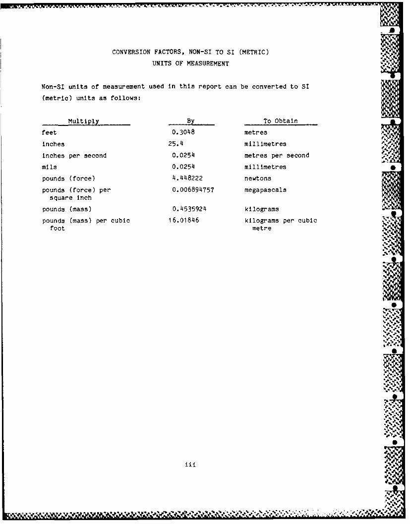
CONVERSION FACTORS, NON-SI TO SI (METRIC)
UNITS OF MEASUREMENT )
Non-SI units ofa measurement used in this report can be converted to SI
(metric) units as follows:
Multiply By To Obtain
feet 0.3048 metres
inches 25.4 millimetres
inches per second 0.0254 metres per second
mi is 0.0254 millimetres
pounds (force) 4.448222 newtons
pounds (force) per 0.006894757 megapascalssquare inch
pounds (mass) 0.4535924 kilograms
pounds (mass) per cubic 16.01846 kilograms per cubic '
foot metre
4
* %
%.Jq-%- %,
.,.p
FAST TRIAXIAL SHEAR DEVICE EVALUATION
CHAPTER I 1
INTRODUCTION
1.1 BACKGROUND
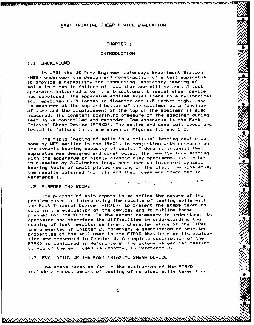
In 1981 the US Army Engineer Waterways Experiment. Station(WES) undertook the design and construction of a test apparatusto provide a capability for conducting laboratory testing ofsoils in times to failure of less than one millisecond. A testapparatus patterned after the traditional triaxial shear devicewas developed. The apparatus applies axial loads to a cylindricalsoil specimen 0.75 inches in diameter and 1.5-inches high. Loadis measured at the top and bottom of the specimen as a functionof time and the displacement of the top of the specimen is alsomeasured. The constant confining pressure on the specimen duringtesting is controlled and recorded. The apparatus is the FastTriaxial Shear Device (FTRXD). The device and some soil specimenstested to failure in it are shown on Figures 1.1 and 1.2.
The rapid loading of soils in a triaxial testing device was Avg
done by WES earlier in the 1960's in conjuction with research onthe dynamic bearing capacity of soils. A dynamic triaxial testapparatus was designed and constructed. The results from testingwith the apparatus on highly plastic clay specimens, 1.4 inchesin diameter by 3.0-inches long, were used to interpret dynamic p.
bearing tests of small plates resting on the clay. The apparatus,
the results obtained from it, and their uses are described inReference 1.
1.2 PURPOSE AND SCOPE I
The purpose of this report is to define the nature of theproblem posed in interpreting the results of testing soils withthe Fast Triaxial Device (FTRXD), to present the steps taken todate in the evaluation of the device, and to outline thoseplanned for the future. To the extent necessary to understand itsoperation and therefore the difficulties in understanding themeaning of test results, pertinent characteristics of the FTRXDare presented in Chapter 2. Moreover, a description of selected e..properties of the soil used in the FTRXD that bear on its evalua-tion are presented in Chapter 3. A complete description of theFTRXD is contained in Reference 2. The extensive earlier testingby WES of the soil used is reported in Reference 3.
1.3 EVALUATION OF THE FAST TRIAXIAL SHEAR DEVICE
The steps taken so far in the evaluation of the FTRXDinclude a modest amount of testing of remolded soils taken from "
I
- ---- ,.-. --- a-- -------- - -,-a

tfte CARES-Dry test site located at Luke Bombing and Gunnery Rangein Arizona and examination of the results of this testing. Theseresults are described in Chapter 4.
An analytical study of a model of the soil specimen as aninitial value-boundary value problem was undertaken to assess theextent of inertial effects on stress at the top and bottom of themodel specimen. A purpose of this study was also to evaluate"gross stress", the stress that is realized when the displacementof the top of the specimen divided by the specimen length isentered as strain into the soil's constitutive relationship. Thepremise of this analysis is that the behavior of the specimenduring rapid testing could be described satisfactorily asone-dimensional wave phenomena in a continuous medium exhibiting.1
realistic, nonlinear, uniaxial stress-strain characteristics. Theinitial values and boundary conditions employed were analyticalrepresentations of the measured conditions during testing. Thisanalysis is presented in Chapter 5. 0
Where inertial effects within the soil specimen are notoverriding, the FTRXD with a soil specimen in it has been modeledas a two degree of freedom lumped mass system. A nonlinear springelement and damper represent the soil specimen; linear springs,dampers, and lumped masses represent the remainder of the device.This modeling work is incomplete and will not be presented inthis report; it will be the subject of a later report.
Future plans call for modifications to the FTRXD for im-proved control of the boundary conditions for the system andimproved measurement of them. Further testing on the CARES-Dryremolded soil and other different soil types will be necessary torefine and validate conclusions drawn from the analytical studiesof the FTRXD. Moreover, to more clearly define the very rapid endof the testing spectrum, further analysis of the soil specimen asan initial value-boundary value problem employing two-dimensionalaxisymmetric wave phenomena with non-linear constitutive behaviorwill be necessary.
' r
N0

Fig 1.1, The Fast Triaxial Device (FTRXD)
mo
ALA
0C
r I'r

.1.............................
A
pMhI"p
P'Iv
Fig 1.2, Failed FTRXD CARES-Dry Specimens
.1~
Am
*1~
I-
~*1~
S
S
I.'.I'.
0
'pSPECIMEAI DATE_________
'p
S
V'p
'p~
0
I.'p.'
-'p....
'4 1~ V~Vd .r'? .~.J J J ,.~ ~ ~ ~ m'.PN ~..............................

p0
CHAPTER 2 lip,
THE FAST TRIAXIAL SHEAR DEVICE (FTRXD) .-81
2.1 THE APPARATUS
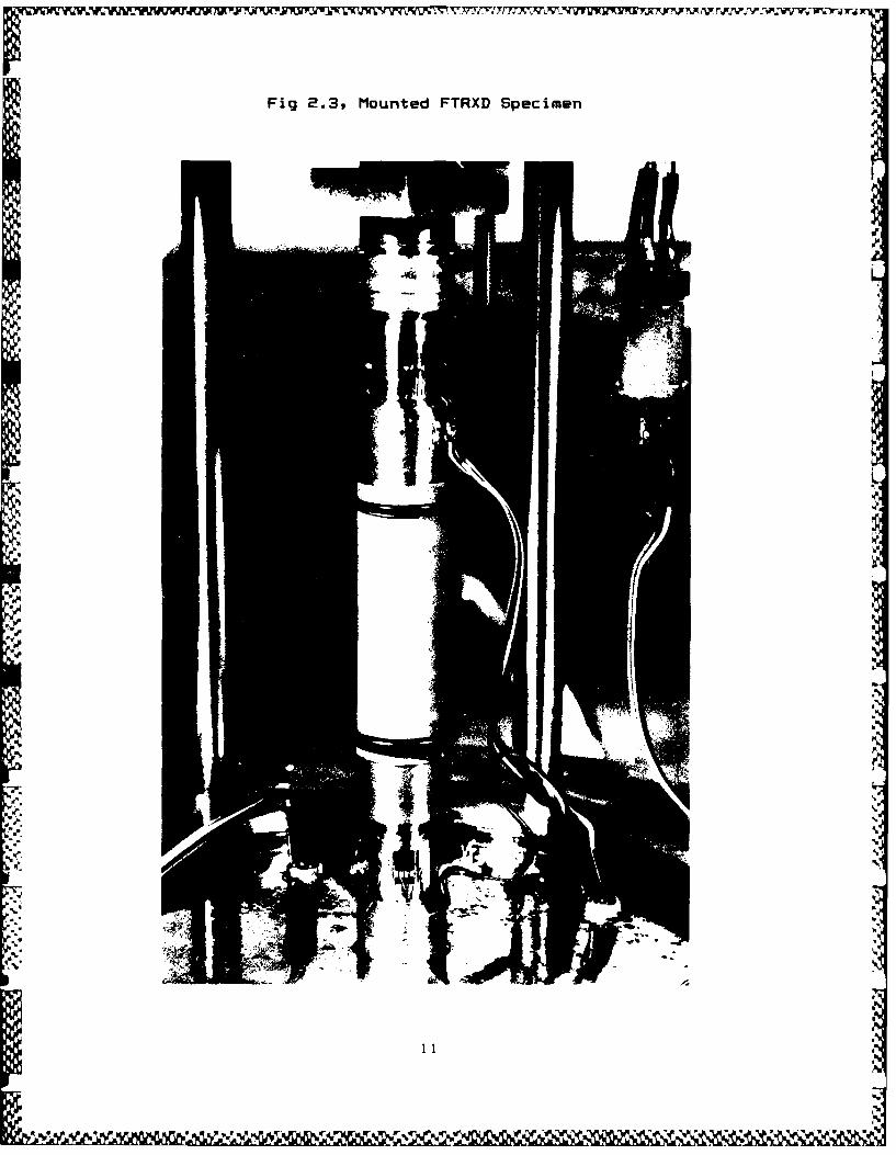
The FTRXD is a triaxial soil testing device. It consists ofa loading assembly, a base, a specimen chamber, a pressurizationsystem, upper and lower load cells, a Kaman gage, and a datarecording system. Schematics of it are on Figures 2.1 and 2.2,photographs are on Figures 1.1 and 2.3, and Reference 2 providesmore complete details.
2.2 THE LOADING ASSEMBLY "4
The loading a-sembly is a piston-cylinder arrangement. Thepiston consists o, a 4.0-inch-diameter steel piston to which isrigidly attached a 0.75-inch-diameter by 7.125-inch-long steel
ram. The piston-ram has a mass of 1100 grams; the mass of the ramalone is about 405 grams. Initially the piston is positioned withits ram in contact with the upper load cell which in turn is incontact with the top of the soil specimen. The chamber in the
cylinder above the piston is pressurized to a pre-determinedlevel using compressed nitrogen. For the slower tests - thodv i-which failure occurs in 20 milliseconds or more - the chamber in :%the cylinder below the piston is filled with oil and sealed untilthe test is initiated. For faster tests, this chamber containsair and is open to the atmosphere, and the piston and ram areheld in position by a tubular shear pin. .
The loading assembly is activated for the slower tests by ..
the rapid ipening of a solenoid valve in the lower chamber of thecylinder which allows the oil to escape. The ability to control ..- ,
the magnitude of the pressure in the upper chamber and the rapidopening of the valve releasing the oil from the lower chamber, •provides a measure of control of the rate and magnitude of theload pulse impressed on the soil specimen. The presence of theoil in the lower chamber flowing from the chamber as the specimenis loaded causes a characteristic shape in the load pulse anddamps undesirable vibrations in the system during testing.
The oil in the lower chamber does not permit the system inits present configuration to bring a specimen to failure in lessthan 20 milliseconds. For faster tests, therefore, there is nooil in the lower chamber. The loading assembly is activated byapplying sufficient pressure in the upper chamber to shear the e
tubular shear pin holding the piston and ram in place. The result.0is a rapid application of load to the soil specimen. A variety oftubular shear pins are available in both aluminum and plastic andwith several different wall thicknesses. The rate of loading is pINincreased by applying higher pressure in the upper chamber abovethe piston and this is made possible by employing strongertubular shear pins.
5
ON0

2.3 THE BASE ..
The base is a steel disk which serves to support the cham-
ber, the lower load cell, and eight studs which in turn supportthe loading assembly.
2.4 THE SPECIMEN CHAMBER
The specimen chamber surrounds the soil specimen and con-
tains fluid subjected to the pressure which equals the confiningpressure for the test. There is a steel or plexiglas chamber for
tests with high or low confining pressures. When testing with the
plexiglas chamber, a wire mesh cylinder is placed around the
plexiglas to serve as a safety shield. The chamber is sealed tothe base and the loading assembly by O-rings and held in place by
the eight studs which also support the weight of the loading Sassembly.
2.5 THE PRESSURIZATION SYSTEM
Compressed nitrogen is the source of pressure used to drivethe piston and ram downward which loads the soil specimen during
testing. It is also used to apply the constant confining pressureto the soil specimen. Two different arrangements are employed:one for the slower tests (times to failure greater than 20
milliseconds) when oil is in the lower chamber of the cylinder
below the piston, and one for the faster tests with no oil in
this lower chamber. A schematic of the pressurization system is
shown in Figure 2.2.
In both arrangements, the confining pressure is applied tothe specimen chamber as pressurized nitrogen over oil and the
chamber is sealed until the test is completed. After the test,
this pressure and the system applying it are used to drain the
specimen chamber of the oil. We.
In the slow test arrangement, pressurized nitrogen is
applied to the oil in the accumulator forcing it into the lower
chamber of the loading assembly cylinder. This provides an
ability to carefully control the positioning of the piston and 0ram and to set it for testing by sealing the lower chamber of the
cylinder. Once this lower chamber is sealed, the pressure on theoil in the accumulator is relieved. Pressure is then introduced -j-
into the upper chamber of the loading assembly above the piston.The test is initiated by the rapid opening of the solenoid valve
to the lower chamber so the oil can return to the accumulator.
In the fast test arrangement, the lower chamber of the
cylinder is left open to the atmosphere. The piston and ram areadjusted manually and set for testing by emplacing the tubularshear pin. Pressure is introduced into the upper chamber above
the ,ston and the test is initiated when the tubular pin shears.
8% a0%% -.. ..
..-. * *.**..* ?~ *'-:-.- * ~. - %

2.6 THE LOAD CELLS
The load cells used in the FTRXD were designed and built atWES. There are four matched pairs of load cells. Each pair
consists of two essentially identical load cells - one which isplaced above the soil specimen during testing (the upper loadcell: ULC) and the other below the soil specimen (the lower loadcell: LLC). The differences between the ULC and LLC are only inthe manner in which they attach to the loading assembly and base.There are four pairs to permit testing with load ranges of 500,
1000, 2500, and 10000 pounds. A photograph of a specimeninstalled between an upper and a lower load cell is shown onFigure 2.3. "
The load cells are stainless-steel cylinders loaded along
their axes. The central part of the load cells are hollow cylin- eders about 0.6-inches long with 0.6 inches for their outerdiameters (the 500-pound set has an outer diameter of 0.575inches). The inner diameters of each set differ to permit in-creasing wall t iicknesses for the increasing load ranges. The 500-and 1000-pound sets have inner diameters of 9/16 inches, the 2500-
pound set's is 1/2 inches, and the 10,000-pound set's is 1/4inches. Two pairs of strain gages are mounted on the outside
surface of each hollow cylindrical part. Each strain gage of the .
pair is located at the midpoint of the cylindrical axis anddiametrically opposite of its mate. One pair is oriented along 0.,
the axis of the cylinder and the other at right angles to i-t. The .four strain gages are equally spaced around the circumference of Kthe load cell. P
A solid cylindrical piece of stainless steel is an integralpart of each load cell and is located between the hollow cylin-
drical part and the soil specimen. It is 0.75 inches in diameterand about 0.5-inches long - a 35 to 40 gram mass. This solidpiece serves as a pedestal directly in contact with the soil
specimen. At the other end of the hollow part are stainless-steelpieces which permit the load cells to be engaged by the loadingassembly (ULC) or attached to the base (LLC).
The 500 and 1000-pound load cells have natural periods ofabout 0.11 and 0.07 milliseconds respectively.
2.7 THE KAMAN GAGE
The displacement of the moving piston and ram with respect
to the fixed part of the loading assembly is measured with theKaman gage and its cantilever target. The Kaman gage is the
KD2300 series displacement measuring system manufactured by KamanMeasuring Systems. It is a variable impedance transducer and is
attached to the stationary underside of the loading assembly. Its Itarget is an aluminum bar 0.385-inches thick by 1.0-inches widerigidly attached to the moving ram as a cantilever. The •cantilever extends 1.625 inches from the edge of the ram to a S
7
% ,:.. "IC

region directly under the Kaman gage. The target for the gage,therefore, is an aluminum surface about 1.625 inches by 1.0 .
inches in plan and 0.385-inches thick. Eddy currents induced inthe moving target result in variations in the impedance in the
Kaman gage. Since the strength of the impedance variationsdepends on the distance between Kaman gage and the target, the
displacement of the target, and therefore of the ram, is sensedand measured. The linear range of the Kaman gage is 300 mils andits static frequency response is 50KHz at -3dB. The manufacturer
also suggests its transient response is 0.01 milliseconds with noovershoot.o
The Kaman gage is designed to perform under static pressures
to 20,000 psi. Confining pressures in the FTRXD are not intended
to exceed 1000 psi. The gage's ability to perform under highpressures and to sense accurately displacements up to 0.1 inches
occurring well within the sub-millisecond range was reported inReference 4. Preliminary analysis of displacement data recordedduring testing with the FTRXD indicates that the Kaman gage can
measure displacement variations at least this fast, meaning its
response time is considerably less than 0.1 milliseconds. Thenatural period in the fundamental mode of the cantilever target,
however, is from 0.20 to 0.30 milliseconds, depending on how the
rigidity of its attachment to the ram is viewed.
2.8 THE DATA RECORDING SYSTEM
An AD509J amplifier was used to generate an excitation
circuit through the Kaman gage and the strain gages of the load
cells. The signals produced by these gages during testing werethus amplified and could be recorded. The AD509J is a high-speed
amplifier exhibiting response times of less than 0.001milliseconds.
A Rascal Stole 7DS tape recorder made a continuous recordof load and displacement data during testing. Magnetic taperecording was employed to obtain high resolution load and .4
displacement data during the very rapid testing. At its toprecording speed of 60 inches/second, the recorder has a time base
error of less than 0.0015 milliseconds and an interchannel time
displacement error of less than 0.0007 milliseconds.
.
S
6 %
BS
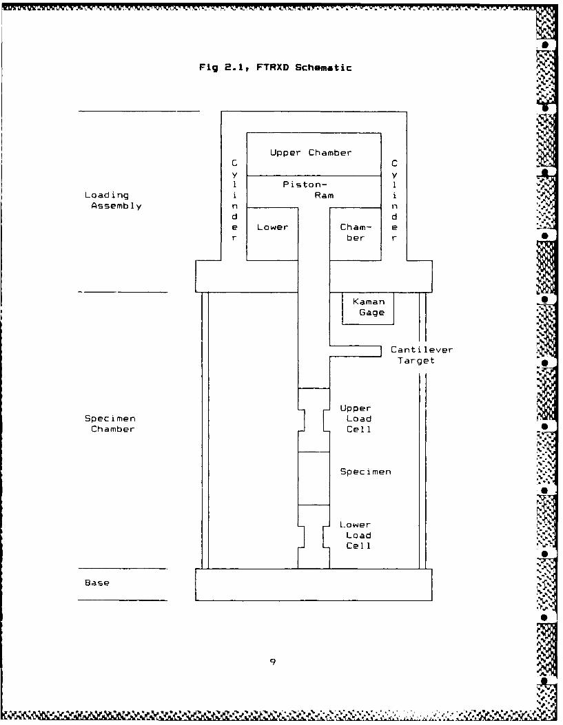
Fig 2.1p FTRXD Schematic %
Upper ChamberC C
y y1 Piston- 1
Loading i Ram iAssembly n n
d de Lower Cham- er ber r
Kaman IGage
CantileverTarget
UpperSpecimen LoadChamber Cell
Specimen
.. .%
Lower
LoadCell
Base , I
9 .P

TV%
,.i
Fig 2.2, FTRXD Pressurization Schematic
(G) (G)V
(X) (G)
(G) (G)
R.
RV
LoadCylinder
( RV ) RV RV () RV I.V
Chamber
Accum- SV Lowerulator X) Chamber
N N FastI I Triaxial
T T CellR R0 0 VG G M- X) - "' .
E EN N
Oi l -Can- s
ister ,
V - Ball Valve
R - Pressure Regulator ARV - Regulating ValveSV - Solenoid ValveP - Pressure Gage
100
101
'AS
~rA '~.A ?~ ~N ~ Vf t17~X'. x.~ ~'d U A~'~ ~ ~ !~) !~ 'V.~ JW JW ~
- Fig 2.3, Mounted FTRXD Specimen
Pr
I
a
a/V.
a-
a
9%
'9
*1*V.9'.,
a-' S.VS.
.9'
9t
a- a
11 9
a-P 9%
'9%
V * 4 ~ W\9q .~' ' .. VI9
-. ' a-
CHAPTER 3
SELECTED PROPERTIES OF THE CARES-DRY SOIL
3.1 DESCRIPTION 1
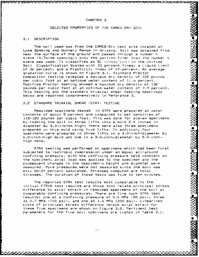
The so", used was from the CARES-Dry test site located atLuke Bombing and Gunnery Range in Arizona. Soil was obtained fromnear the surface of the ground and passed through a number 4sieve (4.76-mm opening); only the portion finer than the number 4sieve was used. It classifies as SC (clayey s-nd) in the UnifiedSoil Classification System with 33 percent fines, a Liquid Limitof 36 percent, and a Plasticity Index of 19 percent. An averagegradation curve is shown on Figure 3.1. Standard Proctor
compaction testing revealed a maximum dry density of 122 poundsper cubic foot at an optimum water content of 11.6 percent.Modified Proctor testing showed a maximum dry density of 132pounds per cubic foot at an optimum water content of 7.9 percent.This testing and the standard triaxial shear testing described
below are reported comprehensively in Reference 3.
3.2 STANDARD TRIAXIAL SHEAR (STRX) TESTING
Remolded specimens tested in STRX were prepared at water %
contents of about 5 percent and compacted to wet densities of118-120 pounds per cubic foot. This was done for eleven specimensby rodding the soil in three lifts into a mold 2.0 inches in
diameter by 5.0-inches high; there were also three specimensprepared in this mold using five lifts. In addition, fourspecimens were prepared in three lifts in a 3.0-inch-diameter by6.0-inch-high mold and one in a 3.0-inch-diameter by 5.0-inch- :
high mold.
STRX testing was performed on specimens which had been first
subjected to isotropic compression under an equal all-around Aconfining pressure. With the confining pressure held constant onthe specimen, axial load was applied to the specimen and theconsequent changes in the specimen's height and diameter weremeasured. Pore pressures were not measured since the soil wasonly 26-29 percent saturated. Stresses computed are totalstresses. The duration of these tests was five to ten minutes. 0
The reported STRX test results most comparable to the
initial FTRXD test results are those that relate principal stress 'difference to axial strain in remolded specimens of the soil atcomparable confining pressures. There are five such STRX testresults: one at a confining pressure of 0.4 MPa (50 psi), three
at 0.7 MPa (100 psi), and one at 1.4 MPa (200 psi). Linearizedplots of principal stress difference versus axial strain forthese five specimens are shown on Figure 3.2. Pertinent test
parameters for the five soil specimens are listed in Table 3.1.e e

3.3 FAST TRIAXIAL SHEAR DEVICE (FTRXD) SLOW TESTING
The soil used initially in the FTRXD was remolded CARES-Dry
soil prepared as 0.75-inch-diameter by 1.5-inch-high specimens,rodded into a suitably sized mold in three to five lifts.Specimen wet densities were 112-119 pounds per cubic foot andtheir water contents were 0.0-4.3 percent. Because these
specimens were smaller than the specimens used in the STRXtesting, only soil passing the number 8 sieve (2.36-mm opening)was used.
Slow testing in the FTRXD was done in much the same manner
as for STRX testing. A constant confining pressure was applied,
the specimen wa loaded axially, and measurement was made ofaxial load and change in the height of the specimen (see Chap 2).The confining pressures employed were 50, 100, and 200 pounds persquare inch and pore pressures were not measured. In the results
reported here for six specimens, test durations were 120 seconds
and 1.2 seconds. Plots of principal stress difference versusaxial strain for these six tests are shown on Figures 3.3 and3.4. Pertinent test parameters for the six specimens are listed
in Table 3.2.
The stress-strain curve for the specimen tested at a
confining pressure of 200 pounds per square inch with a test
duration of 1.2 seconds showed values of principal stress
difference of about one-half of what was expected. The shape of
the curve, however, was as expected. This curve is plotted with u
its principal stress difference values doubled. All of the plots
on Figure 3.3 are pairs of principal stress difference curvesreflecting the readings from both the upper and lower load cells
in the FTRXD. The upper load cell readings consistently plotabove the lower load cell readings in each pair. Though the
difference is small (less than 1.0 percent), it appears to be
larger in the tests completed in 1.2 seconds than those completedin 120 seconds.
3.4 THE LINEAR-HYPERBOLIC STRESS-STRAIN CURVE
Examination of the "static" plots of principal stressdifference (PSD) versus axial strain for the CARES-Dry soil(Figures 3.2 to 3.4) reveals a characteristic shape of the -
curves. They are relatively linear for stress levels up to 20-60%
of the maximum principal stress difference (peak PSD). Thereafter
they exhibit a smooth, non-linear trace with decreasing slope.Some of the curves achieve a peak PSD where their slopes arezero, prior to reaching 15% axial strain. Some do not, however,
especially those at the higher confining pressures. Increasing
confining pressure appears to increase the values of PSD atcorresponding axial strains and to increase the slope of the .k
curves. It also seems to cause the peak PSD to occur at largeraxial strains, or not at all prior to reaching 15% axial strain.These characteristics are not atypical for many soils which
14
41
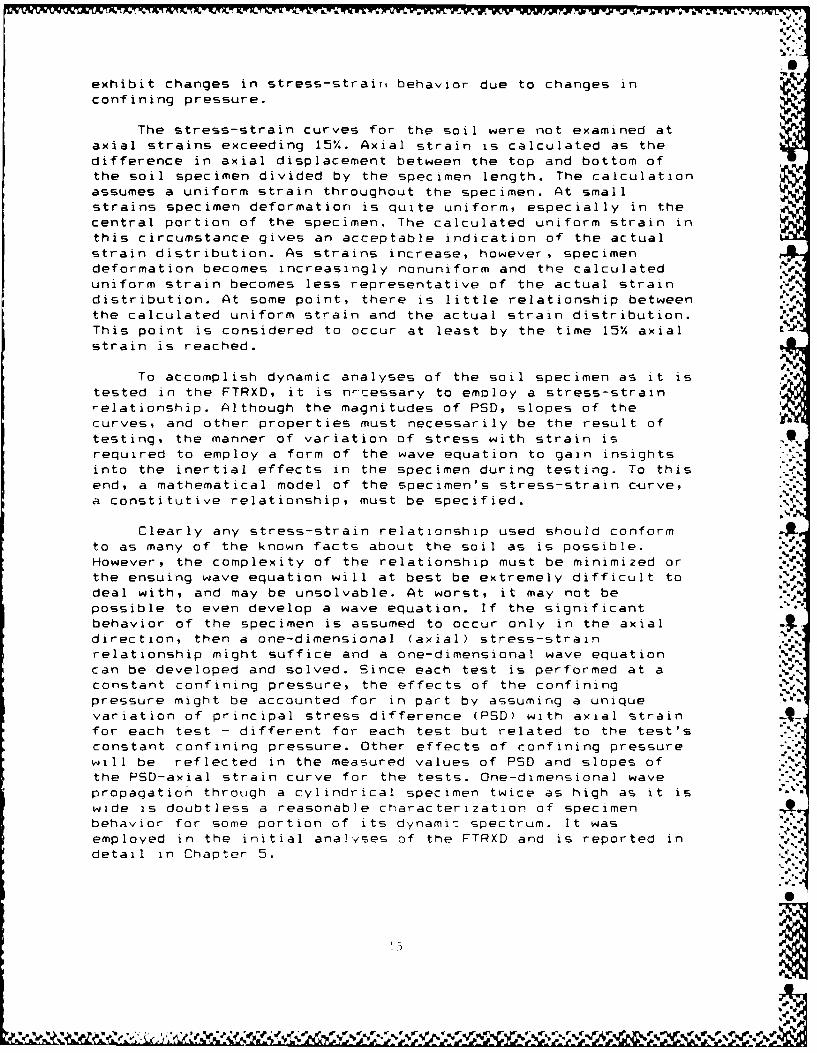
exhibit changes in stress-strairt behavior due to changes inconfining pressure.
The stress-strain curves for the soil were not examined ataxial strains exceeding 15%. Axial strain is calculated as the
difference in axial displacement between the top and bottom ofthe soil specimen divided by the specimen length. The calculationassumes a uniform strain throughout the specimen. At small
strains specimen deformation is quite uniform, especially in thecentral portion of the specimen. The calculated uniform strain inthis circumstance gives an acceptable indication of the actualstrain distribution. As strains increase, however, specimendeformation becomes increasingly nonuniform and the calculateduniform strain becomes less representative of the actual straindistribution. At some point, there is little relationship between
the calculated uniform strain and the actual strain distribution.This point is considered to occur at least by the time 15% axial
strain is reached.
To accomplish dynamic analyses of the soil specimen as it istested in the FTRXD, it is n-cessary to employ a stress-strainrelationship. Although the magnitudes of PSD, slopes of the
curves, and other properties must necessarily be the result oftesting, the manner of variation of stress with strain isrequired to employ a form of the wave equation to gain insightsinto the inertial effects in the specimen during testing. To thisend, a mathematical model of the specimen's stress-strain c-urve,a constitutive relationship, must be specified.
Clearly any stress-strain relationship used should conformto as many of the known facts about the soil as is possible.
However, the complexity of the relationship must be minimized orthe ensuing wave equation will at best be extremely difficult todeal with, and may be unsolvable. At worst, it may not bepossible to even develop a wave equation. If the significantbehavior of the specimen is assumed to occur only in the axialdirection, then a one-dimensional (axial) stress-strainrelationship might suffice and a one-dimensional wave equationcan be developed and solved. Since each test is performed at aconstant confining pressure, the effects of the confiningpressure might be accounted for in part by assuming a uniquevariation of principal stress difference (PSD) with axial strain-4.
for each test - different for each test but related to the test'sconstant confining pressure. Other effects of confining pressure
will be reflected in the measured values of PSD and slopes ofthe PSD-axial strain curve for the tests. One-dimensional wavepropagation through a cylindrical specimen twice as high as it iswide is doubtless a reasonable characterization of specimenbehavior for some portion of its dynamic spectrum. It wasemployed in the initial analyses of the FTRXD and is reported in
detail in Chapter 5.
.* ..

The nature of the experimental PSD-axial strain curves forthe CARES-Dry soil suggests that to describe them in one-dimensional (axial) loading, several parameters are required .
The initial linearity of the curves requires two. The subsequentsmooth nonlinear yielding of the curves with decreasing slopesrequires at least two more parameters. Accounting for the peakPSD when it occurs would require still another. Of the manymathematical functions possible, what was selected and used was asimple straight line for the initial part of the curve from theorigin to a stress level designated the maximum linear stress(MLS). The remainder of the curve was portrayed as a two
parameter hyperbola which smoothly connected to the initialstraight line portion with the initial slope of the hyperbola
equal to the slope of the straight line portion. The hyperbolacontinues to rise with decreasing slopes approaching an upperlimiting stress as strain increases indefinitely. Foridentification, the function is called linear-hyperbolic.
Only three parameters are required to define this functionalrepresentation of stress versus strain. Since the slopes of thelinear part and the initial slope of the hyperbolic part are thesame one parameter is eliminated, and since a peak PSD is notdirectly accounted for another is eliminated also. Of the severalsets of three parameters which could be used, the set chosen was:
- the maximum linear stress (MLS),
- the corresponding maximum linear strain (EL), and- the upper limiting stress (MS).
These three parameters are relatively easy to determinedirectly from an experimental plot of PSD versus axial strain andprovide a good measure of flexibility in fitting a broad range ofexperimental curves. Moreover, the initial linear part lendsitself to an easy beginning for a wave propagation analysis.Figures 3.5 and 3.6 illustrate the linear-hyperbolicstress-strain function. Shown are two sets of four differentcurves. The first set (Figure 3.5) reflects a modest range of .stress levels (MS=400-800 psi; MLS=25, 50, 75, and 100% of MS).The maximum linear strain was arbitrarily set at 2%. The four %
resulting curves exhibit a broad range of curve shapes from thesmoothly yielding lower curve (MLS=100 psi, EL=2%, MS=400 psi) to
the elasto-plastic upper curve (MLS=800 psi, EL=2%, MS=800 psi).The second set (Figure 3.6) illustrates the magnitude of changeof curve shapes that can be effected by varying the parameter ELalone. Comparing the two sets of curves to one another (Figures
3.5 and 3.6), the corresponding stresses in each set of curvesare the same while the maximum linear strains differ.
On Figure 3.7 is reproduced the experimental principalstress difference versus axial strain curve obtained using theupper load cell during FTRXD test RDCFS14 (see Figure 3.3 also).Fitting of the linear-hyperbolic function to this experimental %curve is illustrated on Figure 3.8. The fitting was accomplished
6

by selecting values of the three parameters (MLS, EL, and MS)from a visual examination of the experimental curve. These values
were then used to calculate linear-hyperbolic stress-strainvalues and plot the results. Visual examination of Figure 3.8suggests that the linear-hyperbolic stress-strain plot is anacceptable representation of the experimental curve. The centerlinear-hyperbolic plot seems to be the best fit of the three
h A more refined curve fitting process is certainly possible.
However, first the on-going wave analyses of the test specimen orthe analyses of the test apparatus system should validate theusefulness of the linear-hyperbolic function as representative ofsoil stress-strain behavior. One approach to the curve fitting
process is to define criteria for fitting the mathematicalfunctions to the experimental curves, and then automate theprocess using system identification techniques.
17.
17
* ~ * .~ W %t~r ~ IN

TABLE 3.1
Test Parameters for STRX Testing of Five CARES-Dry Specimens
Test Confining Wet Water Number Mold TestNumber Pressure Density Content of Lifts Size Duration
RDX-TXC-10 50 psi 119 pcf 5.0% 3 2 x 5 5-10RDX-TXC-11 100 psi 119 pcf 4.9% 5 2 x 5 minRDX-TXC-12 100 psi 119 pcf 5.0% 5 2 x 5 doRDX-TXC-13 100 psi 119 pcf 4.9% 5 2 x 5 doRDX-TXC-01 200 psi 119 pcf 5.1% 3 3 x 6 do
TABLE 3.2
Test Parameters for FTRXD Slow Testing of Six CARES-Dry Specimens S%i
Test Confining Wet Water Number Mold Te'stNumber Pressure Density Content of Lifts Size Duration
RDCFS1O 50 psi 113 pcf 4.0% 3-5 0.75 x 1.5 120 sec ,RDCFS14 100 psi 113 pcf 3.8% 3-5 0.75 x 1.5 120 secRDCFS18 200 psi 113 pcf 4.4% 3-5 0.75 x 1.5 120 5ecRDCFS36 50 psi 119 pcf *4.0% 3-5 0.75 x 1.5 1.2 secRDCFS40 100 psi 118 pcf *4.0% 3-5 0.75 x 1.5 1.2 secRDCFS43 200 psi 119 pcf *4.0% 3-5 0.75 x 1.5 1.2 sec
batch value: specimens contaminated by posttest leakage
18
- . -,,S',p%"

.A .
D
Fig 3.1, CARES-Dry Average Grain Size Distriburion
I,6T I MW ,f 6 IOE II I I SW WWMU vol
c - a 3 1 14 1 1 300 4 Io 0 I M 10 M
! it
I I [
IID
s -- - - %
-0 i 0 1 30 i 04 0If
- -s n C fT OR CLY
_ "-ro&NVI L P P1 REMOLDED CARES-DRY SAND
G. - 2.6R
(Average of 3 Data Sets)
GRADATION CURVES __ _
,.,
,£
.5.-
,
16*
Nt19

Fig 3.2, STRESS-STRAIN TEST DATA U
goo DURATiON 5 MIN: RDX-TXC 10, 11, 12,13t,
200 pvt
500-I.
La 400-
100 pal r
40
200 CONFINING PRESSURFE 50 pal
IL 100-
0 1 2 3 4 5 5 7 8 9 10 11 12 13 14 15 15
AXIAL STRAIN ~
20 .~*
Fig 3.3, STRESS-STRAIN TEST DATADURATION 120 SEC RDFCS 10, 14, 18
700-
,. 500
Ii
o 500z
' : Ia1 CONFINING PRESS URE
400
La 300
LL 200-Uz z psiC" 100 -
0-0 2 4 6 8 10 12 14 16
AXIAL STRAIN (%)
Fig 3.4, STRESS-STRAIN TEST DATA
DURATION = 1.2 SEC : RDCFS 38, 40, 4-3700-
.'4. ,--- - -'-
PSDx2 'c1 CP=-Z 500 _
u 500
'-U z. .. -'-U----, - - -
z
ctw CONFINING PRESSU1RE 100 pal
'U. _
4W --
-~-A ~--~ 50 rsi
2200
zCL 100-
0 2 4 5 8 10 12 14 15 18
AXIAL STRAN (M)

Fig 3.5, LINEAR-HYPERBOLIC FUNCTIONSTRESS-STRAIN RELATIONSHIPS
ML.S800 pl. EL!'2.0 X MS=800 pal
-rap
700-
___ ~MLS2!45 psl. ELLO N. M5=500 pal 9...500-
ML"250 pal. ELM2,0 %. MS=
~400-v?
U ___..,_ _--,---"-'9'--
,Jog M..MS=100 pal. EL=2.( "--M------ iwu
200_
100-
o -- e
0 2 4 5 8 10 12 14
STRAIN (N)
Fig 3.6, LINEAR -HYPERBOLIC FUNCTION~oo -STRESS-STRAIN RELATIONSHIPS
sm % %
500 .%
700-
00 //=.'9 ,, E.- 5.0 %. MS=6oo p,'
l//25 palsz~ .EL-- 1.0 %, MS-5oo pa %'0)
0 2 4 6 a 10 12 14 0
STRAIN (%)
22

Fig 3.7, STRESS-STRAIN TEST DATAUPPER LOAD CE.L, TEST RDCIS14
4W0
..5-
3W -
z/61 250-6.La.
J.
5 100-z,
04
2o
0 z 4 5 8 10 1z 14
AXIAL STRAIN ( )
Fig 3.8, TEST & LIN-HYP STRESS-STRAINUPPER LOAD CELL, TEST RDCFS14400 -,
350 p,
Lal 300-uz
% 25 EXPERIMENTALLa.
MLS-2.00 pa, EI-1.4 , MS-400 pal
( 200 MLS=150 pal, EL-1.0 l, MS=425 palMLS-O0 p , EL0.8 , MS 450 pl
1- 150..I.
5 100
zI.
5O,
0 1 T I I I I I I I I
0 2 4 5 8 10 12 14
AXIAL STRAIN C )
23
• " " b, ** ," "," ", , " ",'- , "," "," • "" ", -" ",". -"" ",",' "'" "" "''- ."" "- . ".".", -" ' "" " ","',

CHAPTER 4
PRELIMINARY DYNAMIC TEST RESULTS FROM THE FTRXD
4.1 INTRODUCTION -,
Dynamic tests are those run rapidly enough to begin to causeinertial effects to occur in the specimen, and consequently tomake wave analyses of the specimen of interest. For these
purposes, the dynamic tests were identified as those in which thetest duration was 30 milliseconds or less. The test duration wasconsidered over when an axial strain of 15% was reached in the
specimen. Seven such tests are described here to illustrate thenature of the dynamic test results. Four of the tests werecompleted in 28 milliseconds and three in 2 milliseconds.
Confining pressures of 50, 100, and 200 psi were imposed in boththe 28-millisecond and 2-millisecond duration tests.
4.2 LOAD-TIME DATA
Figures 4.1 through 4.4 show measured load versus time for
the four 28-millisecond duration tests with results from both the i
upper and lower load cells. The confining pressure used is Sindicated and is the only experimental quantity that differs
among the four tests; it is 50 psi for test RDCFS49 (Figure 4.1),100 psi for test RDCFS52 (Figure 4.2), and 200 psi for both. testsRDCFS56 and 57 (Figures 4.3 and 4.4). For some reason, the
magnitudes of upper and lower load readings in these latter twotests was recorded as about one-half of what was expected, just .
as occurred in the slow test on the FTRXD at a confining pressureof 200 psi (see Figure 3.4). Other testing of the CARES-Dry soil
at confining pressures of 50, 100, and 200 psi are the basis forexpecting the load values in these three tests at a confiningpressure of 200 psi to be much higher. The load recorded in all
four tests by the upper load cell was about 12 to 15 percent S
higher than for the lower load cell. Recall that this phenomenonwas also evident, but less pronounced, in the slow tests withdurations of 120 and 1.2 seconds. .
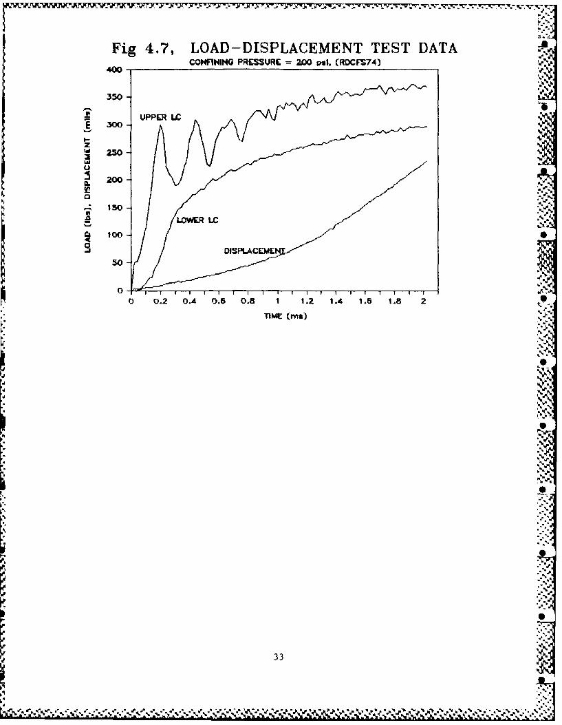
Figures 4.5 through 4.7 show measured load versus time for
the three 2-millisecond duration tests. Confining pressures of 050, 100, and 200 psi were employed on these tests, RDCFS69, 72,and 74 respectively (Figures 4.5, 4.6, and 4.7). The conduct ofthese very rapid tests precluded the use of oil in the lower
chamber of the load cylinder to control and damp the motion of
the piston-ram assembly. In test RDCFS69 (Figure 4.5) where the A
confining pressure was 50 psi, the resistance which the specimencould offer to oppose the loosely controlled motion of the ramseems to have been obscured by the motion of the ram. Thereadings from the upper load cell (which moves with the ram)reflect this strongly. The readings from the stationary lower
load cell are more predictable. The situation is similar, but
25
d
less pronounced in test RDCFS72 (Figure 4.6) where the confiningpressure was 100 psi and the specimen stronger. In test RDCFS74(Figure 4.7) where the confining pressure was 200 psi, thereadings from the upper load cell show a variation one mightanticipate in a very rapid test, while the stationary lower loadcell shows a smooth variation, similar to what was exhibited inthe slower tests. Note the magnitudes of the load cell readingsin this test are about what one might expect rather than halfthat much. Also note the upper load cell readings, at least intest RDCFS74 (Figure 4.7), are on the order of 40 percent higherthan those for the lower load cell. The discrepancy between theupper and lower load cell readings was consistent from the veryslow to the very rapid tests. The upper load cell always readhigher values. The discrepancy also increased significantly fromabout 1 percent for the slow tests to 40 percent for the veryrapid tests.
4.3 DISPLACEMENT-TIME DATA
The measured variation with time of the displacement of the
top of the specimen during the seven dynamic tests is shown onFigures 4.1 through 4.7 along with the load-time variationdiscussed above. The displacement variation is not linear; itcurves upward with increasing slope - more severely the morerapid the test. Displacement-time variation of the top of the
specimen is essential to the wave analysis of the specimen. It is %
taken as the boundary condition at the top of the specimen -sothat displacements, strain, stress, and load can be calculatedthroughout the specimen. Moreover, the displacement versus timedata must permit the calculation of velocities and accelerationswith reasonable accuracy since acceleration and perhaps velocitywill appear in any form of the wave equation employed. One way toachieve this calculation ability is to fit a mathematicalfunction to the displacement data, and then differentiate the
function to obtain velocities and acceleration. Measured velocityand acceleration data along with measured displacement data wouldbe the best approach, but this was not possible at the time thesetests were run.
In tests RDCFS49, 52, 56, and 57 (Figures 4.1 through 4.4),the variation of displacement with time is smooth with anincreasing slope throughout the duration of the test. The curves ,
approach a straight line during the latter part of each test.This variation suggests a function whose slope or velocity beginsat an initial value of zero and then increases smoothly to alimiting value. One might expect such a variation in the FTRXDsince these and all the slower tests were run with oil in thelower chamber of the load cylinder. During the conduct of thetests the piston-ram was initially at rest, the upper chamber of .the load cylinder was under pressure, and the oil in the lowerchamber was under pressure. The test was initiated by rapidlyopening a valve in the lower chamber connecting it to theaccumulator at atmospheric pressure, while maintaining the
26
pressure in the upper chamber. Thus the oil was forced out of the
lower chamber through the opened valve. The piston-ram movedunder the influence of the constant upper chamber pressure andthe lower chamber oil flowing back to the accumulator. The ramtherefore started from rest, its velocity increasing butapproaching a limit since the rate at which the oil could passthrough the opened valve was limited.
A simple mathematical function describing a smoothlyincreasing velocity which approaches an upper limit is a two-
parameter hyperbola. Figure 4.8 shows a plot of the two-parameterhyperbola (velocity), its integral (displacement), and its firstderivative (acceleration). The two parameters needed to definethe curve are its initial slope and its limiting value. Theinitial slope (Ao) is the initial acceleration and its limitingvalue (Vo) is the terminal velocity. Another useful calculated
parameter is the characteristic time (To), which is the ratioVo/Ao. The hyperbola can easily be fitted to the velocity 0variation with time, if good velocity data is available andvaries as described. The fitting procedure is to plot the
reciprocal of velocity versus the reciprocal of time. The resultis a straight line for the hyperbolic function. The slope of thisline is the reciprocal of the initial acceleration (Ao); the
intercept of the line on the 1/V axis is the reciprocal of theterminal velocity (Vo). If the experimental velocity data also
plots as a straight line on these reciprocal axes, the hyperbolicfit is achieved by reading the slope and intercept of the
experimental line.
On Figure 4.9 is reproduced the plot of measureddisplacement versus time of the top of the specimen in testRDCFS56 (see also Figure 4.3). The data were reported at 0.3-millisecond intervals. The displacement was differentiatednumerically with a 3-point central difference expression on a 0.6-millisecond time increment to obtain velocities at intervals of
0.3 milliseconds. The result is also shown on Figure 4.9. Theoscillating nature of the calculated velocity is not easy tointerpret. It probably reflects the effects of dynamics in theFTRXD system, innaccuracies in recording the displacement data,
and the details of the numerical process used in differentiation.Higher order difference expressions and corresponding larger time
increments were tried. They smooth the peaks and valleys of the Soscillations some, but they also seem to change the overall shape
of the velocity-time curve. This overall shape of the velocity 0
curve is apparent on Figure 4.9, and could be represented "o
approximately by the two-parameter hyperbola.
Figure 4.10 repeats the motion data of Figure 4.9 and also S
shows the comparable motion described by a two-parameterhyperbola. The velocity data derived from the experimentaldisplacement data was not good enough to permit fitting thehyperbola to it using a reciprocal axes plot. Consequently, thelimiting velocity, Vo, was estimated by examining the slope of
27 '
o.

the overall displacement plot in the latter part of the testduration. The characteristic time, To, was obtained by tryingseveral values and selecting the one that produced the best .visual fit of both velocity and displacement. The result is shownon Figure 4.10. As with fitting of the linear-hyperbolic functionto stress-strain data, a more refined fitting procedure for the
upper pedestal motion of the FTRXD could be developed. However it
should be justified by the motion data, the wave analyses of thespecimen, and the analyses of the FTRXD system. Moreover, theaddition of accelerometers or other motion measuring devices to
the upper pedestal may be necessary to validate both themathematical functions used and the procedures followed to fit
them to the motion data.
Figure 4.11 repeats the data of Figure 4.10, but adds
acceleration data. Differentiating the measured displacementtwice to obtain acceleration data required smoothing the velocitydata first. The smoothing procedure was to average the elevenvelocity values nearest each time value (the velocity value at
the time value with the five velocity values immediately beforeand after). These eleven values included about one period ofobserved oscillation on each side of the time value. The smoothedvelocity-time variation was then differentiated to obtain
accelerations in the same manner that the displacement-timevariation was differentiated earlier to obtain velocities. Theacceleration data is less meaningful than the velocity data and
affected by the same unknown factors, even more strongly. The
overall variation of acceleration, however, does seem to followthe fitted hyperbolic acceleration which is plotted through it.
Figures 4.5 through 4.7 show the variation of the
displacement of the top of the specimen with time during the veryrapid tests RDCFS69, 72, AND 74. In these very rapid tests the
displacement curves turn up more sharply than in the slower .
tests, especially during the latter part of each test. Recall
that to achieve test durations of two milliseconds, oil could notbe used in the lower chamber of the load cylinder. Consequentlythe motion of the ram in these tests is not restricted by the
flow of oil through a valve.
Figures 4.12 and 4.13 show the results of an analysis of themotion of the top of the specimen during the very rapid testRDCFS74. As with the data from the slower test RDCFS56 (Figures
4.9 though 4.11), the displacement data and the results ofdifferentiating it to obtain velocities are shown. Oscillations
are again present, but the overall variation of velocity withtime is apparent. Clearly in these very rapid tests, a two-
parameter hyperbola cannot be used to describe the motion. The -velocity was smoothed by averaging the thirteen values ofvelocity nearest each time value. The data were reported at time
intervals of 0.02 milliseconds so that the six velocity values on
each side of the time value included approximately one period ofthe observed oscillations. The smoothed velocity variation was
28

"4.
then differentiated to obtain accelerations in the same manner aswas done earlier. Displacement, velocity, and acceleration dataare shown on Figure 4.13. It is worth noting that the calculatedaccelerations are large. The initial spike at 0.05 millisecondsis 2200 g's. The calculated acceleration reaches values of 400
g's several times during the test, and sustains them from about0.9 to 1.4 milliseconds. At this stage in the project no attemptwas made to fit a mathematical function to the motion data of thevery rapid tests. The initial wave analyses used to model these
tests were based on an assumed constant acceleration of the upperpedestal through out the test, which leads to an upward curvingparabolic displacement-time variation.
4.4 DYNAMIC STRESS-STRAIN DATA
The experimentally calculated values of stress versus strain
for the dynamic tests are shown on Figures 4.14 and 4.15. Sincethe stress was calculated from the load cell readings, itnecessarily includes the effects of inertial forces in the
specimen and the dynamics of the FTRXD, if they are present. When 4.
these effects are significant, they will mask the stress-strainproperties of the specimen on experimental plots such as these.
For the tests with a duration of 28 milliseconds (Figure4.14), the relationships are very similar to all of the slower
tests. The differences in the upper and lower load cell readingsare noticeably larger than they were in the slower tests, a-nd themagnitudes of principal stress difference are larger also. These
curves can be represented by the linear-hyperbolic functionequally as well as the slower tests can be, though clearly themagnitudes of the parameters MLS, EL, AND MS would differ. Itwould appear that the 28-millisecond duration and slower tests on
0.75-inch-diameter by 1.5-inch-high specimens of the CARES-Drysoil are not significantly affected by specimen inertia or thedynamics of the FTRXD.
The tests of 2-millisecond duration (Figure 4.15) also show
a similar manner of variation of stress with strain - that is onewhich can be reasonably represented by the linear-hyperbolic
function - when the effects of inertia and system dynamics can bescreened. Figure 4.15 shows the plots of stress and strain for
the very rapid tests using only the stationary lower load cell.For test RDCFS74 at a confining pressure of 200 psi, the curve isremarkably similar to stress-strain curves of slower tests.Recall at this high confining pressure the specimen was strong
enough to not be dominated by the loosely controlled motion ofthe piston and ram. The very rapid tests at lower confiningpressures are also shown on Figure 4.15. Stress and strain doesnot track so well for these tests since the overpowering motionof the piston and ram is evident. Attempting to calculate stress
directly from the upper load cell readings is not meaningful. Themoving upper load cell clearly registered significant inertialeffects of its motion as well as that of the rest of the FTRXD. ".
29
-M I (PF ~ V/Vv W '%V b~~~~. -.

ow -I WT. WT -%r-, -,wv%
Fig 4.1, LOAD-DISPLACEMENT TEST DATACONFINNG PRESSURE = 50 pIl, (RDCF349)32O0
300-
280-
.,250-
240'
i. 220-,2 200
180
IL 150-
o 10 12 16 20 24 2/
20-
TIME UmP) LC
Fig 4.2, LOAD-DISPLACEMENT TEST DATA
CONFINING PRESSURE = 100 pal, (RDCFM52)
300 p
280-
S250-
E 240 -
- 220-z
0. 160-i. 1._60 -, UPPER L WE C/,"
" 't.•; b.
o 140 p E .C
-~120-
- 100"
0 0-0 ISPLACEMENT- 60 •
40-
20-
0- ,
0 4 8 12 16 20 24 28TIME (mes)
300
% %p.

Fig 4.3, LOAD-DISPLACEMENT TEST DATACONFINING PRESSURE = 200 pi, (RDCFWS)
300 /
ao
240220-z
1 200-aL
v o -S 140 . "
. 120 U
=1 100
20 6
40
20'4 '
0 4 8 12 15 20 24 28
TIME (me)
Fig 4.4, LOAD -DISPLACEMENT TEST DATA300-CONFINING PRESSURE 200 pel, (RDCFS57)
280-
.!240-
220-
z 200-
S180-ha
u~140-
.100-'a%
O 50 SPLACEMENT
40-
20 .,
0 4 a 12 18 20 24 28
TIME (me)
31
Z.*'e*0*~

Fig 4.5, LOAD-DISPLACEMENT TEST DATACONFINING PRESSURE = 50 Pal, (RDCF39)
UPPER LC
, 500
IM-
z 400La3°
200
'1001
DI SPLACEMENT
0 0.2 0.4 0,5 0,8 1 '12 114 1 .8 "'
~* 300__-.',
Fig 4.6, LOAD -DISPLACEMENT TEST DATACONFINING PRESURE 100 pal. (RDCFS372)
240-
220-.D 200 >'.5.
-l 100 .,-i'
DISLACMEN
'-a UPPER LC ,
: 120- R' ,
80-
so -- DISPLACEMENT "•"
20 - .. ,
0 0.2 0.4 0.5 0.8 1 1:2 1.4 1.5 1.8 2
,IME " .)
2202
L,%, Ld I ..
*1 I ..
Fig 4.7, LOAD-DISPLACEMENT TEST DATACONFINING PRESSURE 2.00 pi, (RDCF74)
400-
UPPER LIC
z" 250-La
a. 200-
).150,-~ LOWER LC
.'..
~100-0a DISPLACEME
50
61
I~
, 33>

Fig 4.8, HYPERBOLIC UPPER PED. MOTION-o = 10.0 Ip.; To =2.0 me
14 . V --VT/(TO+T)
13- D!EVOT-VOTOLN(1 +T/TO)
12- A=V To/(To+T)"2E 10 -
Am .e ad,'.
IL %
0. 7-J 5LiiL
2L -
4-2-
0 2 4 5 a 10 12 14 15 18 20
TIME (Me)
Fig 4.9, UPPER PEDESTAL VELOCITYTEST RDCFS56
40-
35- CONFINING PRESSURE = 200 pal
30-'._1
ACEM E]T/ 1Z. - .
.j 25
S 20-
10
5-
0 I I jr I
0 4 8 12 15 20 24 z
TIME (e
34
-~r [ m s ) .I
S.*% -- w% .% %'f~ I - C~.~~v..\*a. .. N a
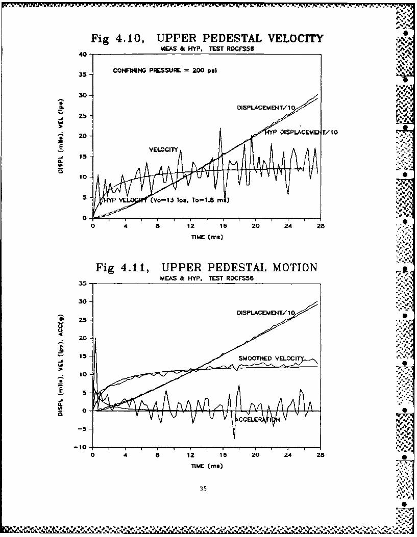
Fig 4.10, UPPER PEDESTAL VELOCITYMEAS & HYP, TEST RDCFS,,
40-
35 CONFINING PRISSURE = 200 pal
30-
DISPLACEMENT/1 0
- '~20YP DISPLACEMFJt T/10
10-
HYP YE (Vo=13 Ips, To=1.5 m )
0 4 8 12 15 20 24 28
TIME (M~e)
Fig 4.11, UPPER PEDESTAL MOTIONMEAS & HYP, TEST RDCF'S56
35- "-
30 5
O 25
20-
- 15- SMOOTHED VE.I'
10p- , ." '
55
CL
-50
0 4 8 12 15 20 24 28
TIME (Me)
35
.%'
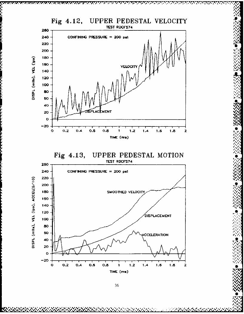
Fig 4.12, UPPER PEDESTAL VELOCITY260 -TEST
RDCFS74
240- CONFINING PRESSURE =200 pil
220o -
20
.j VELOCITY
>. 140-
120-
E 100-
IL
40-
20- PL.AC MENT
0-
0 0. . . . 1.2 1.4 15 .8 2S
TIME (Mea)
Fig 4.13, UPPER PEDESTAL MOTIONTEST RDCFS74
250-
240- CONFINING PRESSURE =200 pal
S220-
200--
L' 180- SMOOTHED VELOCITY
~150
140-A.
.- 120-DISPLACEMENT
Lii 100-
-~80-
E ~ CCELERATION40 S
20-
-20-
0 0.2 0.4 0.5 0.8 1 1.2 1.4 1.5 1.8 2
TIME Cn
36

Fig 4.14, STRESS-STRAIN TEST DATADURATION = 28 me . RDCF 49, 52, 5.
800-
500- t
w 50-CONFINING PRESSUIRE -"100 pal400 /
wr
300 50 PIl..'.
Id / I I 1
o 2 4 5 8 10 12 14 15
AXIAL STRAIN (%) ".,'
Fig 4.15, STRESS-STRAIN TEST DATA,, ;DURATION = 2 me: RDCF 69, 72 74.
700 /% ".
z
IxLd %
u 400-
.. Ip l,.,' a.,
300.
200z
IL 100 /
0 2 4 5 8 10 12 14 15
AXIAL STRAIN ( ) p
70- -3

CHAPTER 5
THE ONE-DIMENSIONAL FTRXD SPECIMEN MODEL
S5.1 BACKGROUND
The FTRXD soil specimen is a right circular cylinder whoseheight is twice its diameter. For static or slow testing, it isassumed to be a differential element of soil exhibiting load and Adeformation characteristics which can be measured and relateddirectly to its stress-strain properties. Displacements, strainand stress are assumed to be uniform throughout the specimen. Thelonger the cylinder is in proportion to its diameter, the lessare the effects of end restraint of the specimen by the testapparatus on the assumed uniform stress and strain distributionwithin the specimen. On the other hand, the longer the specimenis, the more likely is the occurrence of buckling. A height todiameter ratio of 2.0 is usually taken as the compromise thatwill lead to satisfactory static or slow test results. Fordynamic testing an additional consideration is that the longerthe specimen is in relation to the product of its propagationvelocity and test duration, the more noticeable will be the
inertial or wave effects.
The cylindrical soil specimen is failed in shear by %compressing it axially. The specimen shape and testing action .naturally lead to a one-dimensional view of phenomena occurring
during testing. Most triaxial tests are run at a constant lateralconfining pressure so that the application of axial compressiveloads causes one to presume the presence of a controlling
uniaxial stress: the difference between the axial stress and thelateral confining pressure or principal stress difference (PSD).The relationship between PSD and axial strain is what static andslow triaxial testing measures directly. This relationship was
discussed in Chapters 3 and 4 and its representation by thelinear-hyperbolic function described. When triaxial testing is
dynamic, that is when inertial effects and wave phenomena areevident, the specimen can no longer be considered a differentialelement of the soil. The FTRXD attempts to measure the initialvalues and boundary conditions of the specimen. Further analysisis necessary to ascertain any constitutive relationship betweenPSD and axial strain.
There are decades of experience in static or slow triaxial
testing of.soils in which this one-dimensional approach has beenemployed with good success. There is considerable more recent
experience in which one-dimensional wave analyses of triaxial
specimens have been accomplished. These employ a resonant or
standing wave of stress and strain along the axis of the specimenat very low levels of stress and strain. They are carried outwith either compressive or torsional loading and measure eitherrod or shear wave velocities, depending on the loading. They also D
39 Ia'N
a.N
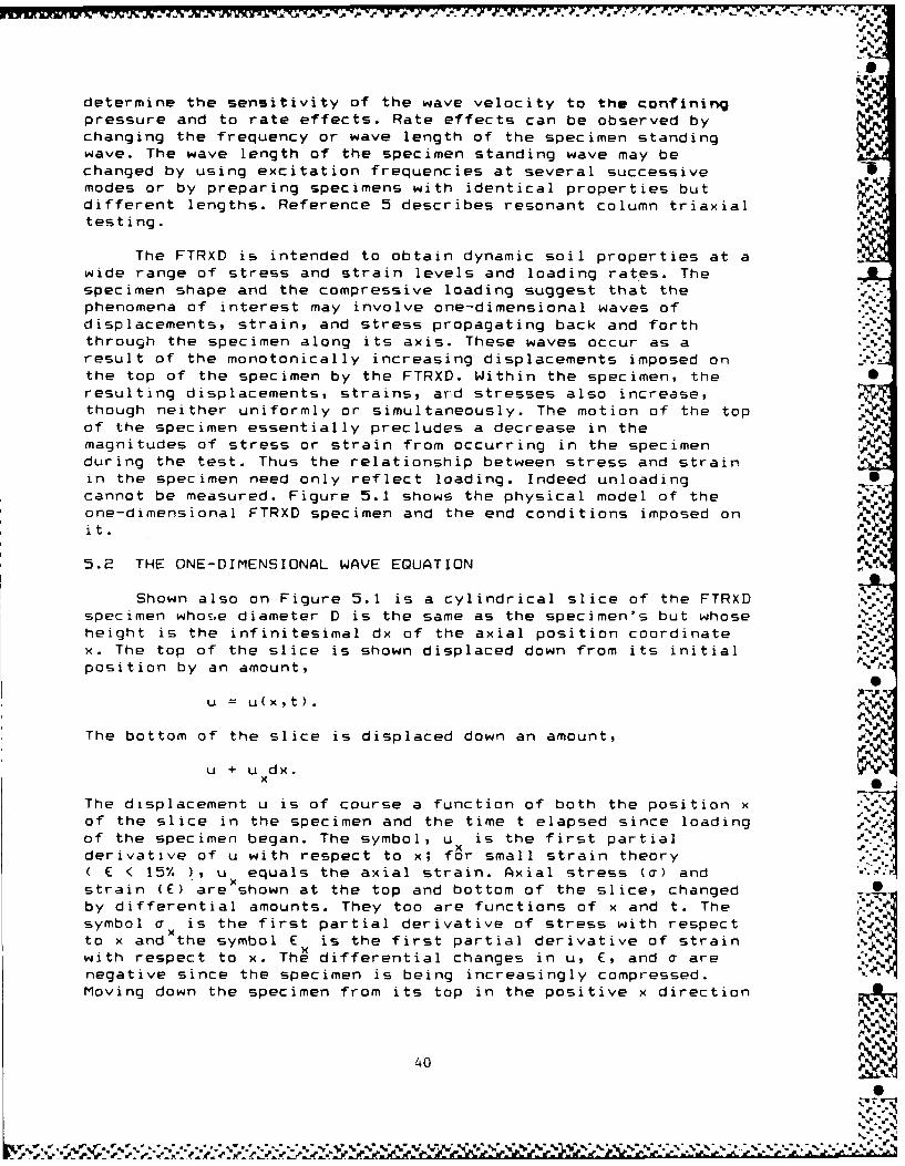
determine the sensitivity of the wave velocity to the confiningpressure and to rate effects. Rate effects can be observed bychanging the frequency or wave length of the specimen standingwave. The wave length of the specimen standing wave may bechanged by using excitation frequencies at several successivemodes or by preparing specimens with identical properties butdifferent lengths. Reference 5 describes resonant column triaxialtesting.
The FTRXD is intended to obtain dynamic soil properties at awide range of stress and strain levels and loading rates. Thespecimen shape and the compressive loading suggest that thephenomena of interest may involve one-dimensional waves of
displacements, strain, and stress propagating back and forththrough the specimen along its axis. These waves occur as aresult of the monotonically increasing displacements imposed onthe top of the specimen by the FTRXD. Within the specimen, the Sresulting displacements, strains, ard stresses also increase,
though neither uniformly or simultaneously. The motion of the top -'
of the specimen essentially precludes a decrease in themagnitudes of stress or strain from occurring
in the specimen
during the test. Thus the relationship between stress and strain .in the specimen need only reflect loading. Indeed unloadingcannot be measured. Figure 5.1 shows the physical model of theone-dimensional FTRXD specimen and the end conditions imposed on M
i t.
5.2 THE ONE-DIMENSIONAL WAVE EQUATION
Shown also on Figure 5.1 is a cylindrical slice of the FTRXDspecimen whoEe diameter D is the same as the specimen's but whose --
height is the infinitesimal dx of the axial position coordinatex. The top of the slice is shown displaced down from its initialposition by an amount,
u = u(x,t).
The bottom of the slice is displaced down an amount,
u + u dx.
The displacement u is of course a function of both the position x '5.
of the slice in the specimen and the time t elapsed since loading
of the specimen began. The symbol, u is the first partial ,..
derivative of u with respect to x; for small strain theoryE < 15% ), u equals the axial strain. Axial stress (a) andx
strain (E) are shown at the top and bottom of the slice, changedby differential amounts. They too are functions of x and t. Thesymbol a is the first partial derivative of stress with respect
to x and the symbol E is the first partial derivative of strain ilwith respect to x. The differential changes in u, E, and a arenegative since the specimen is being increasingly compressed.
Moving down the specimen from its top in the positive x direction
40 0
N

and recalling that the top of the specimen is displaced downwardduring loading while the bottom remains fixed, displacementswithin the specimen decrease and stress and strain becomeincreasingly compressive or negative.
Applying Newton's Second Law to the slice,
(o+u dx)(nD2/4) - a(vD 2 /4) = (gAdx)utt or
x gutt
The symbol u is the second partial derivative of u with respectto the time t it is the acceleration of the slice. The symbol g
is the mass density of the slice and the specimen; it is taken as
constant.
The constitutive relationship is the functional relationship
between stress and strain,
a f(E) so that (5.2)
= (df/dE)(E ) = (f E)(u ) or
= E u where (5.3)X XX
E (=df/dE =da/dE) is the first derivative of f(E) with respectto E; it is the slope of the stress-strain relationship, or thetangent modulus, and is a function of E. The symbol u is thesecond partial derivative of u with respect to x. _
Combining equations 5.1 and 5.3,
(E/g) u = u . (5.4)x x tt
Examining the kinematics of the specimen and slice,
du = (dE)(dx) = (dv)(dt). (5.5) '
The term du is the change in the displacement from the top to thebottom of the slice (through dx) during the time period dt. Thesymbol v is the velocity of the slice during displacement anddeformation; it is equal to the first partial derivative of uwith respect to the time t. The term dv is the change in the
velocity from the top of the slice to its bottom (through dx)during the time dt while the term dE is the change in the axialstrain through dx occurring during dt. Substituting the
appropriate derivatives and differentials into equation 5.5,
(E dx)(dx) = (v dt)(dt) orx t
(E )(dx/dt)(dx/dt) = (v ) or %x t
(u ) (dx/dt)2 = (ut) orx x t t
41
" "
W "IV % -- ----
~~~ a" £1 - Z, q'r%:.jP % 'r % ;1r ~ " ' ~ l' V~--

C2 = U (5.6) .,r
x x t tThe symbol C (=dx/dt) is used for the first derivative of the
position x of the slice (where the differential changes ordisturbances occur) with respect to time. It is the propagationvelocity of the disturbances in the specimen. Comparing equation5.4 with equation 5.6,
C2 = Elg. (5.7)
Equation 5.6 is the one-dimensional wave equation where C isthe rod wave velocity. When C is constant, E must be constant '.
dimensional Hooke's Law ( a = EE ). When the linear-hyperbolic
constitutive relationship is in effect, E is a function of strainonce the maximum linear stress o. (MLS) and corresponding maximumlinear strain E (EL) are reacheA. The propagation velocity inthe specimen, therefore, is a function of strain (equation 5.7)also. Equation 5.6, then, becomes the one-dimensional 6
linear-hyperbolic wave equation.
5.3 THE ONE-DIMENSIONAL LINEAR-HYPERBOLIC WAVE EQUATION
Figure 5.2 illustrates the linear-hyperbolic stress-strainfunction discussed in Chapter 3 and shown on Figures 3.5 and 3.6.The cur've plotted on Figure 5.2 is the lowest of the four plottedon Figure 3.5. The equations defining it are,
= E E when E < E and (5.8a) •01
(E-E(_)= when E > E (5.8b)
(I/E )+(I/o )(E-El) '0 h1*. 4
where, •= axial stress, E = axial strain, %
a' = maximum linear stress (MLS),
a = maximum stress (MS),max
ah= maximum hyperbolic stress (MS-MLS),
El = maximum linear strain (EL), and
E = slope of the linear part of the function andWo initial slope of the hyperbolic part.
When E<€I'E
da/dE = E = E and0
C2 = C2 E/g
42
me ep0

Substituting into equations 5.4 or 5.6,
(C)2 u u (5.9)0 xx tt
Equation 5.9 is the linear one-dimensional wave equation.
When E>E 1 (l/E
da/dE = E = 0 so that,[(1/E )+(l/ h )(E-E 1)J2
(a /E )2h 0 o -
E/E h(5.10)EI 0o [ (( h /E )+(E-E )]2 -. 5
Recalling equation 5.4,
(E/g) u = u andxx t
(1IE )(E/g) u = (1/E ) u . (5.11)0 xx 0 tt
Substituting equation 5.10 into 5.11,
(a hE ) 2u = (g/E ) u (5.12)
[(r /E )+(E-E )]2 0 tt
Rearranging and recalling that
C 2 = E /g and that E u
the linear-hyperbolic one-dimensional wave equation for E>Ei may .be written,
u• uxx ut t 'xx .____=____(5.13)
[(a /E )+(u -E )]2 CC a /E ]2h o x 1 o h o
40 5.4 THE FINITE DIFFERENCE GRID
Equations 5.9 and 5.13,
ut
for E< E u - tt (5.9)
(C 2~
0u u
xx (C )
for E>E (5.13)1I ((h /E )+(u - I )] 2 [C a /E 2
h o x 1 oh 0N
are a system of second order two-dimensional partial differentialequations. They are linear for strains (u ) less than E , and
x 1
43
%0

nonlinear for strains greater than E . They can be solved 1%14numerically for displacements, u(xptf, by replacing the partialderivatives of u(xt) with respect to x and t with finite
difference expressions.
Central difference expressions are convenient, accurate, andwell-suited to the wave equation. Three-point formulas are thesimplest possible when second derivatives are present and they
provide suitable accuracy as long as the finite difference grid
is sufficiently fine. The grid is made up of points in the x-tspace which are equally spaced in each coordinate direction. Thedifference between any two successive points in the x direction,
Xmmand x M 1 is the spatial increment Sx. Similarly, thedifference between any two successive points in the timedirection, t and tn, is the time increment St. The index m
refers to position anb the index n to time. Thus, ,
xm = (m-l)&x, m=1,2,3, ......
t = (n-l)&t, n=1,2,3, ......n
The central difference expressions are centered" on the point(x ,t ) in x-t space, and are identified and located by thei n2ces (m,n). Three such expressions are required,
u - Um+l ,n Um-l ,n ...a)x 26x
u -2 u + u
u - m+ln m,n m-1,n (5.14b)x x2
um,n.l -2 u + um n l m 9n M .-u (514c)ut t " •
The terms subscripted by the indices m and n are the values of
the displacements at the corresponding five points identified inx-t space by the indices as,
(m-, n)
(mn-1) - (m n) - (mn+l)
x (m+ ,n)
-
44
SqS - ~ ~ ? % % I - -w -. 4P 'P 5 -4.' .

The times of the initial arrivals of the incident andreflected waves at a point in the specimen are determined by theinitial propagation velocity C of the specimen and the distance
the waves have propagated through the specimen to reach the
point. These times of arrival plot as straight lines in x-t space .
with slopes equal to C , or in dimensionless (x/h)-(C t/h) spacewith slopes equal to one. The symbol h is the height of the
specimen. Figure 5.3 illustrates the dimensionless (x/h)-(C t/h)
space in which Sx has been set equal to C at and both are equalto 0.10. The horizontal lines of points define position lineswithin the specimen (x=x ) which begin at the initial times ofmarrival of the incident wave. The vertical lines of points are
time lines (t=t ) which also plot only after the initial arrival
of the incident wave. The sloping lines are the plots of initialtimes of arrival of the incident and reflected waves at pointsthroughout the specimen. Only three traverses of the initialarrivals of waves are shown: the incident wave first propagating
down through the specimen; the first reflected wave propagatingback up through the specimen after reflecting off its bottom; and
*the second reflected wave propagating back down through thespecimen after reflecting off its top. The tic marks shown locate
the points (x ,t ) which may be identified with theirM
corresponding ingices (m,n). Figure 5.3 is referred to as the
finite difference grid.
5.5 THE FINITE DIFFERENCE ALGORITHM
Substituting the difference expressions (equations 5.14)into the linear 1D wave equation (equation 5.9) results in,
u r -2u +U u -2u +uC ln m,n m-,n m,n+l m,n mn-lC 2 =o0r 6,
0 5x2 &t2 .
C Stu 0 )2 (u 2 u +u + 2u - um.nm,n+l -m+lon- mon+m-l,n mon m,n-I l,
(5.15a)
Equation 5.15a can used to calculate the displacement at grid %
point (m,n+l) provided that the displacements are known at grid
points (m,n), (m+l,n), (m-l,n), and (m,n-l). With respect to Npoint (m,n+l), these four points each are located at it, aboveand below it by an amount Sx, and earlier than it by amounts St
or 26t as illustrated below.
45 N 'f % NN %4N N -W '
%
t 1 t t n5n-i n+ n+l S.
_+ + +_______ t 1
x r-I (m-1,n)
xrn + (mn-1) - (m n) - (m,n+l)
"m+1 (m+Jn)
x .
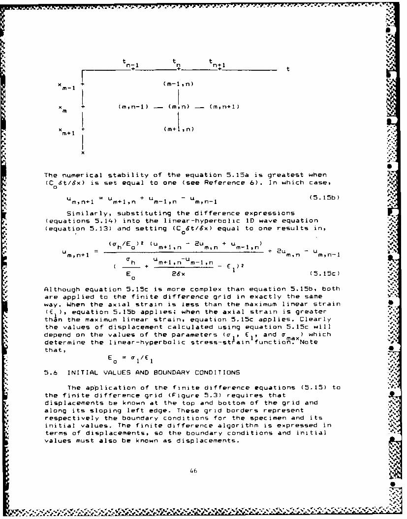
The numerical stability of the equation 5.15a is greatest when(C 0 t/Sx) is set equal to one (see Reference 6). In which case,o
u -+ n u (515b)m,n+1 m+l,n Um-l,n m,n-
Similarly, substituting the difference expressions(equations 5.14) into the linear-hyperbolic ID wave equation(equation 5.13) and setting (C ot/Sx) equal to one results in, "4
* 0
(a/E)2 (u- + u Weum,n+1 h 0 um+l,n -rn ,n M-mn + 2umn - m,n-1
h + m-,n m-),n E )2
E 26x (5.15c)o %%Although equation 5.15c is more complex than equation 5.15b, both
are applied to the finite difference grid in exactly the sameway. When the axial strain is less than the maximum linear strain(EI), equation 5.15b applies; when the axial strain is greaterthan the maximum linear strain, equation 5.15c applies. Clearlythe values of displacement calculated using equation 5.15c willdepend on the values of the parameters (a,' E., and amax ) whichdeterrine the linear-hyperbolic stress-strain function. Note "',
that,E /- /%
o l 1
5.6 INITIAL VALUES AND BOUNDARY CONDITIONS 1
The application of the finite difference equations (5.15) tothe finite difference grid (Figure 5.3) requires thatdisplacements be known at the top and bottom of the grid andalong its sloping left edge. These grid borders representrespectively the boundary conditions for the specimen and itsinitial values. The finite difference algorithm is expressed in kterms of displacements, so the boundary conditions and initialvalues must also be known as displacements.
46k "L
S..
,.-- _ -.-. .-.-.-.-.- , ---. , .- ,. -, , .-.- ,. *' w .',. . .,? %. . v %.*,, , ... . .. ?' i . *r. .,-,r%, -, ., %.
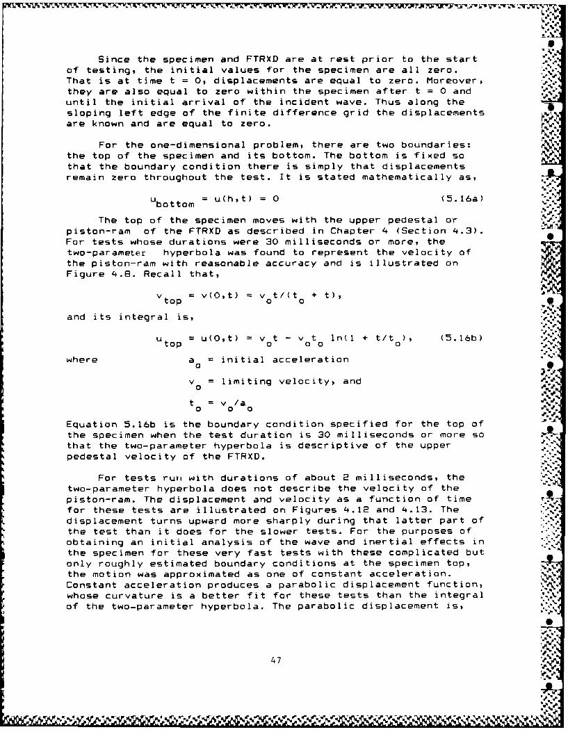
Since the specimen and FTRXD are at rest prior to the startof testing, the initial values for the specimen are all zero.That is at time t = 0, displacements are equal to zero. Moreover, .
they are also equal to zero within the specimen after t = 0 anduntil the initial arrival of the incident wave. Thus along thesloping left edge of the finite difference grid the displacementsare known and are equal to zero.
For the one-dimensional problem, there are two boundaries:the top of the specimen and its bottom. The bottom is fixed so Vthat the boundary condition there is simply that displacements
remain zero throughout the test. It is stated mathematically as,
% ~Ub to = u(h,t) = 0 (5.16a) ..
The top of the specimen moves with the upper pedestal or .vpiston-ram of the FTRXD as described in Chapter 4 (Section 4.3).For tests whose durations were 30 milliseconds or more, thetwo-parameter hyperbola was found to represent the velocity of
the piston-ram with reasonable accuracy and is illustrated on
Figure 4.8. Recall that,
vto p = v(O,t) = v t/(to + t),
and its integral is,
u = u(O,t) = Vot - v t ln(1 + t/to), (5.16b)top o 0 0 0
where a = initial acceleration
v = limiting velocity, ando
t 0= V0 /aa% o o 0'
Equation 5.16b is the boundary condition specified for the top ofthe specimen when the test duration is 30 milliseconds or more sothat the two-parameter hyperbola is descriptive of the upperpedestal velocity of the FTRXD.
For tests ruti with durations of about 2 milliseconds, thetwo-parameter hyperbola does not describe the velocity of the
piston-ram. The displacement and velocity as a function of time -
for these tests are illustrated on Figures 4.12 and 4.13. The
displacement turns upward more sharply during that latter part ofthe test than it does for the slower tests. For the purposes ofobtaining an initial analysis of the wave and inertial effects inthe specimen for these very fast tests with these complicated butonly roughly estimated boundary conditions at the specimen top,the motion was approximated as one of constant acceleration.Constant acceleration produces a parabolic displacement function,whose curvature is a better fit for these tests than the integral
of the two-parameter hyperbola. The parabolic displacement is,
47

utop u(O,t) = (a t2)/2 = (v t2)/(2t ) (5.16c)0o0 0
where a = constant acceleration,o A N w
0Av = velocity of the specimen top at the time
0the incident wave first reaches thebottom of the specimen,
t = time at which v is reached.0 0
Equation 5.1bc is the boundary condition specified for the top ofthe specimen for the very short duration tests in which equation5.16b is not satisfactory. Note the constants v and t are
0useful constants which are descriptive of the upper peaestalmotion, but which have different interpretations for equation5.16c than for equation 5.16b.
The upper pedestal motion of the FTRXD (boundary conditionof the top of the specimen) is an essential part of the analysis.Different results are obtained if the upper pedestal motionchanges. In describing the results of analyses of the FTRXDspecimens later in this chapter, the corresponding upper pedestalmotions will be illustrated also.
5.7 FINITE DIFFERENCE DISPLACEMENTS
The finite difference algorithm (equations 5.15) may bie %viewed as a pattern in the x-t space of the finite difference
grid. When the displacements at the four grid points shown belowat times t and t are known, the displacement at the grid point * ..at time t can be calculated. The calculations would be started
4
1 2 3 4 5 n
+ 1,3) _- + + -
2 + (2,2) - (23) - (2,4) +
3 (3 3) + +
4 +. +
m x
by centering the pattern on grid point (2,3), which has spacetime coordinates (Sx,26t). The displacement at (1,3) is knownfrom the boundary condition at the top of the specimen; the %
displacements at (2,2) and (3,3) are known from the initialvalues in the specimen. What is missing is the value of thedisplacement at grid point (2,3). Indeed, all the displacements
48
%0
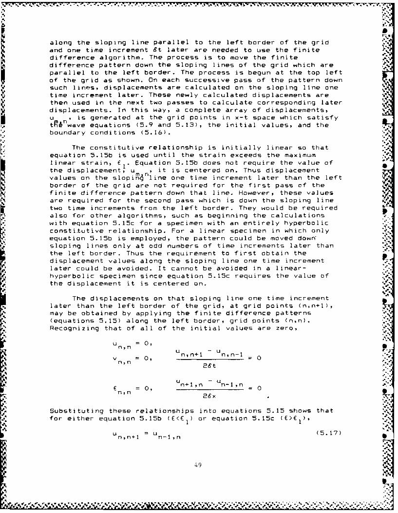
along the sloping line parallel to the left border of the grid
and one time increment St later are needed to use the finitedifference algorithm. The process is to move the finitedifference pattern down the sloping lines of the grid which are
parallel to the left border. The process is begun at the top left
of the grid as shown. On each successive pass of the pattern down
such lines, displacements are calculated on the sloping line one
time increment later. These newly calculated displacements arethen used in the next two passes to calculate corresponding later
displacements. In this way, a complete array of displacements,
u , is generated at the grid points in x-t space which satisfy
tpLnwave equations (5.9 and 5.13), the initial values, and the
boundary conditions (5.16). '1'
The constitutive relationship is initially linear so thatequation 5.15b is used until the strain exceeds the maximum ..
linear strain, E Equation 5.15b does not require the value of- 1*
the displacement, u , it is centered on. Thus displacement
values on the slopinline one time increment later than the left
border of the grid are not required for the first pass of the
finite difference pattern down that line. However, these valuesare required for the second pass which is down the sloping line
two time increments from the left border. They would be requiredalso for other algorithms, such as beginning the calculationswith equation 5.15c for a specimen with an entirely hyperbolic
constitutive relationship. For a linear specimen in which onlyequation 5.15b is employed, the pattern could be moved down"
sloping lines only at odd numbers of time increments later than
the left border. Thus the requirement to first obtain the
displacement values along the sloping line one time increment
later could be avoided. It cannot be avoided in a linear-
hyperbolic specimen since equation 5.15c requires the value ofthe displacement it is centered on.
The displacements on that sloping line one time increment
later than the left border of the grid, at grid points (n,n+l),may be obtained by applying the finite difference patterns
(equations 5.15) along the left border, grid points (n,n).%: Recognizing that of all of the initial values are zero,
u =0,n,n •,u - u a.,
v =0O, n,n+1 n,n-1 = 0 'n,n
u -u
~n~nn=n+1 n,nEU1n+l,n n-l,n 0f
Substituting these relationships into equations 5.15 shows that
for either equation 5.15b (E<Ei) or equation 5.15c (E>Ei),
= u (5.17)n,n+1 n-l,n
49
r' W orv*** .1 r''.VV~ % W........

I'
Equation 5.17 is the starting equation for the finite differencealgorithm. It states that the displacements along that slopingline one time increment later than the left border of the grid .
are each equal to the displacement of the top of the specimen onetime increment after it begins to move. -
5.8 FINITE DIFFERENCE STRAINS AND STRESSES
The algorithm and starting equation, equations 5.15 and A5.17, are the basic tools required to obtain the solution to the %wave equation, the array of displacements, u , in the x-t spaceI mnof the finite difference grid. However, the m gnitude of thestrain at each step in the calculations must be monitored todetermine whether the linear or hyperbolic part of the specimen'sstress-strain relationship is in effect. That is, strain E mustbe calculated and compared to the maximum linear strain l andequation 5.15b or 5.15c invoked as appropriate. 1.
In general, strain may be calculated with the three-pointcentral difference expression (equation 5.14a) used to developthe finite difference algorithm (equations 5.15), or
u -um+ln m-,n (5. b)
m,n 2&x
The displacements at (m+l,n) and (m-l,n) are known just prior toemploying the algorithm to calculate the displacement at (m,n+l).The algorithm is center-based also, centered on (mn). Thus E mCnis calculated (equation 5.14b), compared to EI, and equation m5.15b or 5.15c used as appropriate. 1
The array of displacements, u, once generated, is neededto calculate the strain at a pointm n the specimen as a functionof time. The stress at that point as a function of time then maybe calculated using the specimen's stress-strain relationship(equations 5.8). The stresses at the top and bottom of thespecimen are the ones most directly related to the force measuredby the upper and lower load cells of the FTRXD. Therefore thestrains at the top and bottom of the specimen must be calculatedfrom the displacement array to obtain these stresses.
At the very top and bottom of the specimen, centraldifference expressions cannot be used for the strain calculation.Instead, forward difference expressions, focussed on the gridpoints at x = 0 (m=l), are neccessary for the strain at the top.Backward difference expressions, focussed on the grid points atx = h, are necessary for the strain at the bottom. Since centraldifference expressions are more accurate than forward or backwarddifference expressions, four-point forward and backwardexpressions were employed in an effort to maintain the same levelof accuracy that the algorithm possesses. •.
50 %
%S

*, Referring to the finite difference grid (Figure 5.3), thestrain finite difference expressions were not allowed to extendover the sloping lines which mark the initial arrivals of theincident and reflected waves. The displacements and strainsimmediately adjacent to either side of these lines can differsignificantly, especially if the specimen has been loaded with a
pulse approaching the severity of a step pulse. Thus near thegrid points where the sloping lines intersect the top and bottom
*i of the grid, the four point forward and backward differenceexpressions could not be used. At the first grid point on either
side of the intersections, two-point formulas were used; at thesecond grid point on either side of the intersections, three-point formulas were used. At the other points on the top andbottom of the grid, the four-point expressions were used. Thetwo, three, and four-point forward and backward differenceexpressions employed were (Reference 6),
x1 x2 x3 x4
&x u (x1 -1 1 - -x I
Sx u (x ) 1 -i - -
x u(x) -3/2 2 -1/2Sx u (x) 1/2 -2 3/2 -
x3
Gienth u (x ) -11/6 3 -3/2 1/3 (51%S x u x (x1) -1/3 3/2 -3 11/6 (5.1)N
5.9 DIMENSIONLESS VARIABLES AND PARAMETERS
Given the three parameters required to define the linear-hyperbolic constitutive relationship of the specimen (E , a , and
E ), the specimen length (h) to identify the geometric sizemoftIe specimen, the mass density of the specimen (g) to quantifyinertia in the specimen, and the two parameters (v and t ) todefine the upper pedestal motion or boundary condiTions o the
specimen, direct calculation of displacements using equations
5.15 will produce an entire array of displacements in x-tspace for each set of values of these seven parameters. If eachparameter were to assume only four values, 16384 such arraysmight be calculated. For finite difference grid points separatedspatially by one-tenth of a specimen length, each displacementarray might contain 4000 displacement values (lOxlOx40). Theresult, of course, would be an enormous volume of displacementdata. However, combining the sevenI parameters into dimensionlessgroupings and setting the finite difference grid so that Sxequals C 0't, reduces the number of parameters to three so that0
the number of arrays will be reduced to a small fraction of thenumber that would be required otherwise (64 vs 16384). That is,only three dimensionless parameters would be required todetermine dimensionless displacements in dimensionless space andtime.
51 4k
S...

x s..t,: ; ..- _ - :, -.' &×, := - '- - .- . . - *V . . -. . -.- . . : .- - A
Dimensionless space z is taken as the ratio of the spatial Ncoordinate x to the specimen length h. Dimensionless time T istaken as the ratio of elapsed time t to the time required for theinitial wave to propagate the length of the specimen. Thus,
z - x/h and (5.19)
= C t/h where (5.20)
C = 4(E /g) ando o
E T= /o 1 l
The upper pedestal displacement for a hyperbolic upper pedestalvelocity was seen earlier to be,
U to p v t - v t ln(l + t/t ) (5.16b)
or, U = T T 0 In( + i /) where (5.21a)
dt to0 0Udt =(U top/h) (Co/vo)
= C t /h, So o o .
t v /a,o o 0
v = limiting upper pedestal velocity, and
a = initial upper pedestal acceleration. 0o
For constant upper pedestal acceleration,
u = (V t2)/(2to) (5.16c)top o 0
or, U = -r2/2 where again (5.21b) S
u = (u /h)(C /v ), butdt top 0 0
v = a h/C , and.0
a.
a = constant upper pedestal acceleration. •
Consistent with equations 5.21 dimensionless displacement is,
Ud = (u/h)(Co/Vo). (5.22)d 0 0
Dimensionless strain is determined as,
E (u u )/z -z) ord d2 dl 2 1
(u /h u /h)(C /v )/(x /h x /h)2 1 0 0 2 1
Ed " (C /Vo) (5.23) S
52 P, % wS..'
5e,., ,- ; .- y j & 4 2..A.wa'4' ~.* * '.""
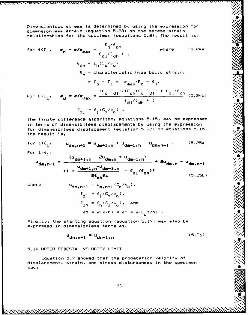
Dimtensionless stress is determined by using the expression for
dimensionless strain (equation 5.23) on the stress-strain
relationships for the specimen (equations 5.8). The result is,
E d/E dhfor o< w wradh where (5.24a)frd "max =E /E + 1
dl dh -
E dh = h (Co0 /V)
E = characteristic hyperbolic strain,
E -E o /E -E0 1 max 0 1
(E - E )/(E +E - E + E~ /EF d dl dh d dl + Cdl dh (52.
For E>E l , rd iq/Wqx = /E (5.24b) Cdl /dh + 1
S=E (C /vdl 1 0 0
' F
The finite difference algorithm, equations 5.15, may be expressed
in term tof dim nP 4 dp1Ptm~nti hy wnq thP P~prerion 'Nfor dimensionless displacement (equation 5.22) on equations 5.15. %.9
The result is,
for E< , Udmn+l = Udm+lpn + Udm19n Udmpn-l (5,5a
For C>E , . 'WU - Eu +u )
- (Udm+ln dmn dm_1 ,n _2u--
dmn+l dmon dmyn--U -Udml pn dm-1,n /Ed).
h+2 EdZ dl dh (5.25b)
where U dm,n+l m n+ (C a o/ 0
C = E (C /V),dl 1 o o
Cdh Ch (Co/v ), and %
6z = 6(x/h) = 6T = (C t/h) . •a
Finally, the starting equation (equation 5.17) may also beexpressed in dimensionless terms as,
Uu( 5.2P6)".,_,Udnvn+l Udn-lyn
5.10 UPPER PEDESTAL VELOCITY LIMIT
Equation 5.7 showed that the propagation velocity ofdisplacement, strain, and stress disturbances in the specimen
was, S
53
% %-
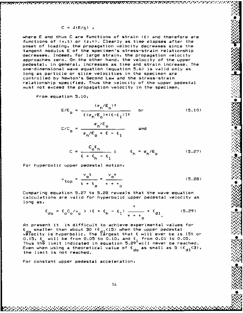
~I.%
C = 4(E/g) , ..
where E and thus C are functions of strain (E) and therefore are
functions of (xt) or (zr). Clearly as time elapses after theonset of loading, the propagation velocity decreases since thetangent modulus E of the specimen's stress-strain relationship
decreases. Indeed, for large strain, the propagation velocityapproaches zero. On the other hand, the velocity of the upperpedestal, in general, increases as time and strain increase. Theone-dimensional wave equation (equation 5.6) is valid only aslong as particle or slice velocities in the specimen are
controlled by Newton's Second Law and the stress-strainrelationship specified. Thus the velocity of the upper pedestalnust not exceed the propagation velocity in the specimen.
From equation 5.10,0(ah/E ) 2
E/E = o ________ or (5.10)
0 [(a /E )+(E-E )]2h o 1
a h /E 0
C/C = o and 0crh/E o + E'E
C o E ..
C oh h = h/E (5.27)
h 1
For hyperbolic upper pedestal motion,
v t v i
v t 0 (5.28)
t + t 0 + S
Comparing equation 5.27 to 5.28 reveals that the wave equationcalculations are valid for hyperbolic upper pedestal velocity aslong as, 'A
E = IC /v > (E + Ch - E 1) + Edl (5.29)do 00 o h 1 + T
0%
At present it is difficult to achieve experimental values for
C smaller than about 30 (E <15) when the upper pedestaldl % .1veocity is'hyperbolic. The Vargest that E will ever be is 15% or
0.15, E will be from 0.05 to 0.10, and E from 0.01 to 0.05. 0o 1
Thus the limit indicated in equation 5.29 will never be reached.Even when using a theoretical value of Edo as small as 5 ( dl<3),the limit is not reached. d
For constant upper pedestal acceleration,
54
40

v top a t =v . (5.30)
Comparing equation 5.27 to 5.30 reveals that the wave equationcalculations are valid for constant upper pedestal accelerationas long as, -
E E C /v > (E +E E +E(.1do o o + h - l T + Edl (5.31)
To date, experimental values of E of about 20 have beenachieved with a constant upper pegestal acceleration. Smallervalues might also be possible. A theoretical value as small as 5(with a constant acceleration of about lO0Og and E = 2.5) isuseful to illustrate the limitation imposed by equa ion 5.31.Taking the largest reasonable E (=0.15), E (=0.10), and the
0corresponding E (=0.05), the wave equation calculations would bevalid until at least a dimensionless time T of about 12. Howeverfor these test conditions, that 15% failure strain will bereached in a dimensionless time of about T=8 so that again thelimit expressed in equation 5.31 will not be reached.
5.11 PROGRAM FTSP 'a?
The one-dimensional linear-hyperbolic wave equation was 0solved in dimensionless terms employing equations 5.21, 5.25, and5.26. Dimensionless strain and stress at the top and bottom of -'the specimen were calculated from the resulting dimensionlessdisplacements using equations 5.23 and 5.24.
To compare the calculated top and bottom stress, whichaccounts for one-dimensional inertial effects in the specimen,with the stress usually derived from triaxial testing, a third
astress, termed gross stress was also calculated. Gross stress isthe stress obtained when the displacement of the top of thespecimen divided by the length of the specimen is entered asstrain into the specimen's constitutuve relationship. The strain Sso used is termed gross strain. Gross stress and strain wereobtained in dimensionless form using equations 5.21, 5.22, 5.23,and 5.24.
The equations were coded for solution on a computer in AFORTRAN (F77) as Program FTSP. A complete listing of Program FTSP 0is contained in Appendix A. The code runs interactively with aminimum amount of input required from the keyboard. The boundary- 'conditions are established by providing a value for Tr , one ofthe three dimensionless parameters. ',
T = C t /h = 0, for a step velocity and linearly0 O0 0increasing displacement of the
the upper pedestal,
'o > 0, for hyperbolic upper pedestal velocity, and0
T 1000 for a constant upper pedestal acceleration. 00
55V
I % -W
*t W 'r~~
The finite difference grid is defined by specifying thenumber of increments which the specimen length is divided into
and the duration over which the calculations will be made.Specifying the number of increments allows the calculation of Sz
and ST. The duration is set by stating the maximum even integervalue of T. For slow tests (duration = 28 milliseconds) in whichS(=C t/h) was about 125 at E=15%, good numerical accuracy wasachieved with Sz=0.10. Rapid tests (duration = 2 milliseconds),in which T was about 9 at E=15%, required 6z=O.05 to achievesatisfactory numerical results.
Finally, values for the remaining two dimensionless
parameters, t (= E C /v ) and a/ la (= MLDS), are entered.
The program tngenerates an array mf imensionless displace-ments in dimensionless space and time, and calculates the
dimensionless top, bottom, and gross stress and strain.
Program FTSP was compiled with the Microsoft FORTRANCompiler (version 3.3) both with and without a math coprocessor.With the coprocessor, the compilied code requires 295 kilobytes
of random access memory and takes 1-3 minutes for one data run onan IBM PC/XT. Without the coprocessor, 302 kilobytes of random
access memory are required and a data run takes 7-15 minutes. Thebulk of the random access memory requirement occurs because FTSPis written to accomodate up to 50 increments in a specimen length(Sz=0.02) and up to 1000 dimensionless time steps (maxT=10006z).
A sample run from Program FTSP is contained in Appendix B.In this run, •
0 = C t /h 5.0,
Edo C /v = 10.0,
1(l max MLDS = 0.25,
S z = ST = 0.05, and -'
max T = 40.0
5.12 SPECIMEN TOP, BOTTOM, AND GROSS STRESS -..
Figures 5.4 through 5.20 are plots of the top, bottom, andgross stress data generated by Program FTSP and illustrations ofthe details of the upper pedestal motion used. The plots attempt
to portay a spectrum of specimen behavior as the values of thedimensionless parameters change. Five values of 0 were used tovary the upper pedestal boundary conditions. These were,
T= 0.0 step velocity pulse, "V..o e rl= 5.0 extremely rapid hyperbolic velocity,- 10.0 very rapid hyperbolic velocity, .
= 20.0 rapid hyperbolic velocity, and= 1000 extremely rapid constant acceleration. S
56

Six values of Ed were used to reflect a range of ,constitutive behavior of the specimen from soft to stiff relativeto the rapidity with which the specimen is loaded. These were,
E = 5.0do-10.0
= 20.0 p= 30.0
40.0
In general for a given test rate (v ), the stiffer specimens havehigher values of C (E C /v ) than the softer specimens do.
do 00a 0
Only one value of a./c (= MLDS = 0.25) was used. Thisparameter essentially relecT the overall shape of the specimenstress-strain curve which translates directly into the overallshape of stress-time or stress-gross strain plots.
Figures 5.4 to 5.7 show the stress-time and stress-grossstrain behavior of a FTRXD specimen subjected to a step velocitypulse of upper pedestal motion. The motion is simple; the top ofthe specimen displaces linearly with time so that plots of stressversus time are identical with plots of stress versus grossstrain. The step velocity pulse, however, is a very severe d%
loading of the specimen in the initial phases of the test. Itrequires an enormous acceleration for a very short time at thebeginning of the test. Consequently, significant inertialeffects occur at the arrival of the incident wave and eachreflected wave at each point in the specimen. Though the stepvelocity pulse cannot be achieved presently in the FTRXD, it isincluded here because it illustrates clearly the differences inthe top, bottom, and gross stress due to inertial effects.
On Figures 5.5, 5.6, and 5.7 the gross stress plots as asmooth linear-hyperbolic stress-strain curve. The stress at the -N
top of the specimen jumps instantaneously to a value comensuratewith the step loading and a wave propagates into the specimen.The disturbance propagated is a change in strain proportional tothe step velocity imposed on the specimen top. The change instrain may be interpreted as a change in stress using thespecimen's constitutive relationship.
The stress at the bottom must await the arrival of theincident wave (at 7=1.0). Because it is reflected off the rigidstationary lower pedestal, the stress at the bottom of the .
specimen jumps instantaneously at T=1.0 to a value equal to twicethe value of the stress change in the incident wave. A similar Sevent occurs at the top of the specimen when this first reflectedwave arrives there (at T=2.0) and is reflected off the rigiddownward moving upper pedestal. The stress at the top thenincreases instantaneously by an amount equal to twice the value J,
of the stress change in the incident wave so that stress
57%-
,%.

at. the top now becomes equal to three times the value of the %stress change in the wave. The process repeats at each subsequent V
initial arrival of the wave at the top and bottom of the %d
specimen, increasing the stress there each time by an amountequal to twice the value of the stress disturbance in the wave. -s
In the early part of the test when stress varies linearlywith strain, the process is clear and simple and is illustratedon Figures 5.5, 5.6, and 5.7. When stress and strain begin their -nonlinear relationship, the stress change in the wave as aconsequence of the strain change is progressively smaller, inconformity with the nonlinear stress-strain relationship. Thesmaller stress change means that less resistance can be offerred
to the inertial forces so that the severe step pulse on itsarrival causes an overshoot and minor oscillation as it reflects.These phenomena are evident in the figures. The smaller stress
change also means that the stresses at the top and bottomincrease by progressively smaller amounts on each reflection.This latter result causes the stress-time and stress-gross strainto display a nonlinear shape characteristic of the specimen'sstress-strain relationship.
Clearly in a test with a large enough step velocity pulseimposed to cause failure (E=15%) to occur within just a few wave
traverses of the specimen (say T=10), the top, bottom, and grossstress. would differ greatly. However if the top and bottom
stresses were carefully plotted, a curve drawn through the 'theirintersections would trace the specimen's actual stress-strain
relationship quite reliably. Such plots could be made by plottingupper and lower load cell readings divided by an appropriate areaagainst the gross strain (upper pedestal displacement divided bythe specimen length).
If the specimen were more slowly loaded so that failure didnot occur until after many traverses of the wave, the differences
among top, bottom, and gross stress would be insignificant, andperhaps not discernible. Then either the upper or lower load cellreadings divided by the specimen area and plotted against thegross strain could be used directly as the specimen's stress-strain relationship.
The overshoot and minor oscillation observed with the step
velocity pulse on each reflection after the stress and strainlevels in the specimen became high enough to exhibit a nonlinearrelationship, technically invalidate the data displayed. The
finite difference algorithm and Program FTSP have no provisionfor stress-strain unloading. This is because except for the step S
pulse, unloading was not anticipated and never observed.Moreover, this unloading (the oscillations) with the step pulseis thought to have little effect on the important aspects of theanalysis. An unloading routine could be incorporated into ProgramFTSP, but it would enlarge the memory requirements for the code
.0
and increase its computation time. It does not appear to bejustified at this time.
Figures 5.8 through 5.15 show the top, bottom, and grossstress in specimens subjected to hyperbolic upper pedestal -velocities. The Figures 5.8 to 5.11 are for T =5.0, the fastest
0hyperbolic loading of a specimen shown. A hyperbolic upper Vpedestal velocity with a characteristic time t =0.9 millisecondimposed on a 1.5-inch-long specimen whose rod wave velocity is700 ft/sec would have T =5.0. At t=0.9 milliseconds half itslimiting velocity would0be reached; three-quarters of itslimiting velocity would be reached by t=2.7 milliseconds. Evenso, the top, bottom, and gross stress-time plots shown are muchless severe than they were for the step pulse. There is noovershoot and the differences among the top, bottom, and grossstress are much less.
Figure 5.10 shows the first quarter of Figure 5.9 expandedfor closer observation of the early part of the loading.Differences among top, bottom, and gross stress are evident and %perhaps would need to be accounted for. To observe stress-grossstrain behavior, Figure 5.11 graphs the second highest curve ofFigure 5.10 (do =10.0) as stress versus gross strain. Gross
stress plots as a linear-hyperbolic function as expected whiletop and bottom stress oscillate in a minor way above and below
it. Because the velocity of the upper pedestal and thus thestrain and stress changes in the propagating wave are nonli'near,the top and bottom stress oscillations about the gross stressline are not symmetric as they were for the step velocity pulse.Nonetheless, a trace of the intersections of the top and bottomstress still provide a good representation of the specimen's
actual stress.
Figures 5.12 and 5.13 are for T =10. The curve for E =30 onFigure 5.13 corresponds to the 28-millisecond duration tesas runon the FTRXD and shown on Figures 4.1 to 4.4, 4.9 to 4.11, and4.14. Clearly within the one-dimensional model of the specimen,there is little difference in the values of top, bottom, or gross
stress. The differences evident on Figures 4.1 to 4.4 and 4.14 inupper and lower load cell readings are probably not attributableto inertial or wave effects within the specimen. Instead, theyare more likely the result of the dynamic behavior of the FTRXDas an assemblage of deformable components possessing mass and theinstrumentation employed during testing.
Figures 5.14 and 5.15 portray the behavior of a specimenwhose upper pedestal velocity has T =20.0. From the point of viewof wave propagtion, these results are essentially static.
The truly dynamic tests were those run rapidly enough toshow significant inertial and wave effects. The fastest tests runto date were those whose durations were about 2 milliseconds. The ."
results of these tests are shown on Figures 4.5 to 4.7, 4.12,
5 '
0-

_-F. W*. vr w'iwL 0- 0. -_ PUJ -V rv -r
4,13, and 4.15. The upper pedestal motion of these tests wascomplex and could be only roughly estimated (Chapter 4, Figures4.12 and 4.13). Consequently, constant acceleration of the upperpedestal, a simple approximation of this motion, was used for theanalytical study of the inertial effects in the sample under veryrapid loading. Figures 5.16 through 5.20 show the results of this
study. Since only one parameter is needed to define the upperpedestal boundary condition instead of two, only twodimensionless parameters are required for the stress-time datainstead of three. These are a /a (= MLDS = 0.25) and E (E C /v = 5, 10, 20, 30, 40, 1 5W Note that for constant00 0upper pedestal acceleration, v is the velocity of the upper
pedestal at the instant that tee initial wave reaches the bottom J,of the specimen; it is not a limiting velocity as in the case ofhyperbolic upper pedestal velocity.
The curves for Edo =20 are the closest approximation for the2-millisecond duration tests run on 1.5-inch-long specimens ofthe CARES-Dry soil. These are replotted on Figures 5.18 and 5.19to T=10, the dimensionless time at which E is approximately 15%for constant upper pedestal accelerations of 300 to 400g (seeFigure 5.16). Examination of Figure 4.13 suggests that the •2-millisecond duration tests might be approximated using constant %upper pedestal accelerations of from 300 to 400g.
Gross stress plots as a smooth curve between top and bottomstress as expected, and as the linear-hyperbolic function on thestress-gross strain plots of Figure 5.19. There are cleardifferences among the three stresses. Top stress plots entirelyabove gross stress and bottom stress entirely below it. The onlyexceptions appear to be at T=2 and 7=4 where all three stressescome together.
Figure 5.20 shows the curves for E =5 plotted to T=8. A S1.5-inch-long specimen whose rod wave veocity is 700 ft/sec and rwhich is subjected to a 1200g constant acceleration of its top,might possess E =5. In addition, C=15% would be reached in about
do1 millisecond or T=8 and v =83 in/sec. The differences among top,0
bottom, and gross stress are clearly much greater for this muchmore rapidly loaded specimen. Nonetheless, gross stress plotsagainst gross strain as a linear-hyperbolic function, the correctconstitutive relationship for the specimen. It is bounded by top '1stress above it and bottom stress below it as it was in Figure5.19. Though neither top or bottom stress by themselves representthe specimen's constitutive relationship well, some functionalcombination of the two could be found which would. No attempt wasmade to find such a functional relationship since it is not clearyet whether constant acceleration for the upper pedestal is themost reasonable representation of the upper pedestal boundaryconditions for the very rapid tests. 1
The clear differences between the upper and lower load cellreadings and the significant oscillations in the upper load cell
i
.,
Jq,
60. Z:W

readings as shown on Figure 4.7 for the 2-millisecond duration
test, RDCFS74, cannot be explained from the specimen's dynamic
behavior alone. They presumably reflect the dynamic response of
the FTRXD itself and perhaps the instrumentation employed.
%, %
6 , ',.- s
,-A,_
,*7S'
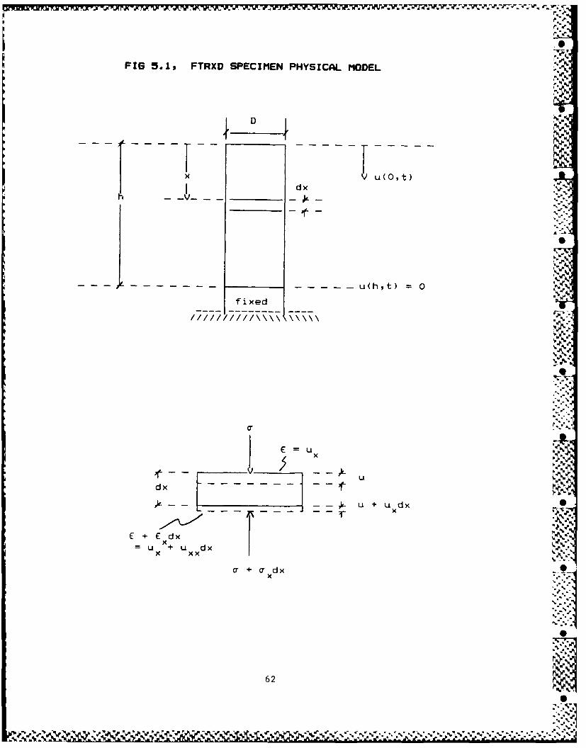
FIG 5.1, FTRXD SPECIMEN PHYSICAL MODEL -
x dx u(Ost)
- - -- - - -__ - - uht
A
E u x
kVdx
-- u u+ udxx
E + E dx=U x + u x~
*+ a dxx
62
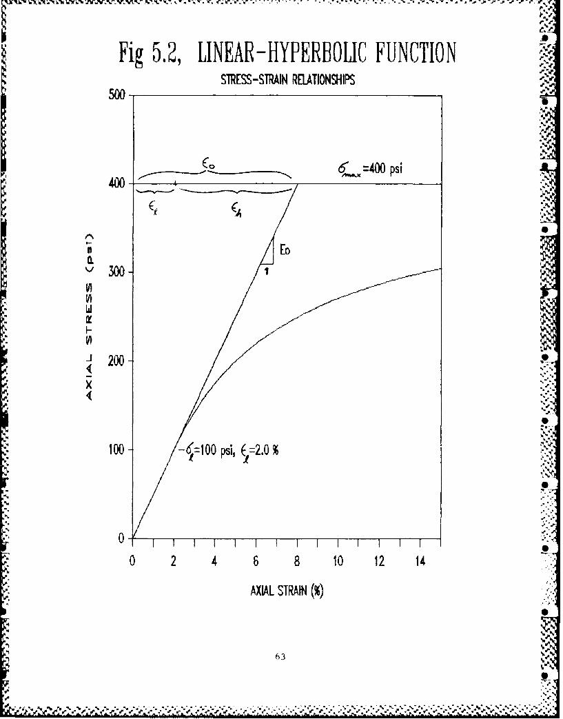
For;..
ig 5.2, LINEAR-HYPERBOLIC FUNCTIONSTRESS-STRAIN RELATIONSHIPS .0
500-
60., =400 psi
400* ______
n' EoLA/h"
-'200-
100 -6%100 pd, 20 %
AXIA STRAI (%)
63
X.::F-

f. r
44-
Q + + + + + + + bf
+ + + 4 + +
+ + + ++ +
+ + + ++ + + +
['1 N
+
C )r
d. 6 I'e
+ 4X- + O I~ + +1+ + + +4hi
Z64'

Fig 5.4, UPPER PEDESTAL MOTIONHYPERBOUC DIMENSIONL... PI,TS40 I ' r,
Coio/h 0.0 35-s30 - (=15X.t V0------ IIp e
o" .- %-t
25 (--15%t, Y0-=50QI/'/
_ 20o(=19C vo= lip*-- ,.-.,° 7
15 DISPLACE MENTi -.. ''E- VELOCITYxl 1
10-
9.
0 10 20 30 40i,--
TIMIE (C01/11) or' GROSS STRAIN ((Cc/Vo) ,. w
Fig 5.5, TOP, BOTTOM, & GROSS STRESS ,CotO/h =0.0 MLDS =0.2."5'
O 15 -ISPA"EMNT0.9
-, VOflC, i 1
0.8- (oco/Vo=5
0.7-
:~'.4
0. -. % ".,
(A 0.6 - -"
" 0.5- I
w4 0.4 -.
C,,/- =00.0-MLDS-, 0.2
z0.
U) 0. -
\ 0.2
U).: ...0.14
U) 0
0 10 20 30 40 0
TIME (COt/h) or GROSS STRAIN ((Co/Vo)
U)1
65I
0.55U)
U)\| ~

Fig 5.69 TOP STRESS & GROSS STRESS otI
0. (C/Vrn5 CQIQh =0.0 MLD' = 0.2Z5 40.
10 J0,0
2000.5 .0 MD =02
11 -4
0.4-0
0 .
'-0.5-
TIM (CIh .GOS TAN(~/b
0.4
(A 0.3 "1in
1. 0.25S
a4ul 0.4 -
0 02 0400
0-0
0, 10 20-..- 30 40-.-.
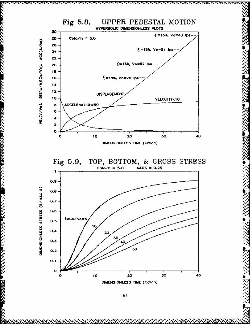
Fig 5. 8, UPPER PEDESTAL MOTIONHYPERBOUC DIMENSION' ESS PLOTS
za 2- Cole/h 5.0 f=15%. Vo=43 ia-
S 25-
L) 24- E=15%, o=51 Ips--
1 2(A 20 PLACEME
al ACEL.ERnOCx5
61>
12
0 DI0P20CEM0 40
0.7-.
(A 10 2 04
C0/ = 0 MD .
i 0.3-4
z2 0 .7 - 5 0
0.10.5
0z '
0 0.20304DIESOLS TM Cth
z6i %]

Fig 5.10, TOP, BOTTOM, & GROSS STRESS07Coto/h 5. ML S O
0.5-
.t 0.3-
0.
% 0.3
0zU),/ 0.2 MD 02
LA'
LAIo/ 0..025- 02
(A 0.5-
0< 0.35 0
w 0.31
0.25 -1
U) 00 34
DIESOLS RS TAN2C/o
~ 0.15
ez

Fig 5412, UPPER PEDESTAL MOTIONHYPERBOUC DIMENSIONLESS PLOTS
24-
0- 22- Coo/h =10.0 4 Ve%5 Ip-
20 £1s~.vo=63 1ps--
A 15- =1 50 Vo=75 lp-- 7
14-
S 12- f=15%, Vo=101 lpv -
In DISPLACEMENT
VELOCI1'Vx 1 . .
6- \ACEERTp.x
4-
> 2
010 20 30 40
DIMENSIONLESS IME (Col/h) I.p
Fig 5.18, TOP, BOTTOM, & GROSS STRESSCotlo/h =10.0 MLDS =0.25
1-
0.IhL
U\ 0.7-
U) 0.5 - o
S0.5-(AU)
w 0.4 -EoCoAo=5
0u0.3-2
z 32 0.2 -
0.1 :yI0 10 20 30 4 0
DIMENSIONLESS TIME CCoi/h)
69 p
p o

Fig 5.14, UPPER PEDESTAL MOTION A
HYPERBOUC DIMENIONIS PLDTS15 0-
150- o -0 -/h 20.0 =I v0=8 1p
4140-
.13 = =9 Ia-. -Io Az j.' ¢:o 120 A
C=15, vo=1 1 -,--
110-
100- E =I" Vo-13 IP.-
go-
70 /5a DISPILACEMENT
50- VELOCITYx5O
40 S
~30-20 "
10 ~ LRATIONxSO0
0 20 40 50 80 100 120 140 150 180 200 S
DIMENSIONLESS TIME (Cot/h)
% ,,
Fig 5.15, TOP, BOTTOM, & GROSS STRESSCoto/h = 20.0 MLDS 0.25
0.9 (EOco/vo=5
0.820
4 0.70
0.7-
0.5La
U' 0.5 -
1 0.4- ON.
z0.3 -
z
2 0.2-
0.1
0 - 1 F I-I I I I I I 1 l I I I I I II
O 20 40 50 80 100 120 140 150 180 200
DIMENSIONLESS TIME (Co-/h)
700
~ ~I* .~yI.%.X~ -~V V ~ .~.. . .NO -

Fig 5.16, UPPER PEDESTAL MOTIONPARABOLIC DIMENSIONLESS PLO0TS
20ig- NOTE: Vo Is mool a Ilmrnng vtellty
0 Is5 Yo = A)(h/Co)17- A* ConO4ant
O 15 VELOCITY
14-
12 -,
11 - ACCELERATIONx 1010- (=15% Ao~lg--
7-,
E=I56 Ao=143g--"
5- =IW~ Ao=187g-
21 .7 ElaK AOM400- -- DISPLACEMENT/20
'I 2 4 5 0 1 1~4 1'5 185 20
DIMENSIONLESS IME (Co&I/')
Fig 5.17, TOP, BOTTOM, & GROSS STRESSU.P. ACCEL =A* MLDS =0.25
1.-
tA 0.8 E oCo/Vo=s
(A 0.6-U) ."
'- 0.5-
CA
0.4-z
FA 0...'.
z
0.2 0
0.1
0 2 4 6 8 10- 1 12 114 i6 18 20
DIMENSIONLESS TIME (ColA,)
71
%a
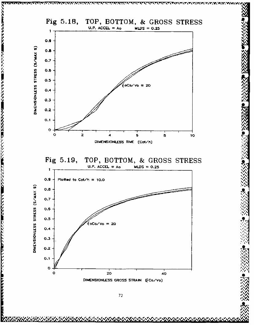
Fig 5.18, TOP, BOTTOM, & GROSS STRESSU.P. ACCEL = Ao MLDS = 0,25
0.9
0.5
_ 0.7
t - 0 .1 -
0 . 5 E c ek v o 2 0
0 pzLaA
2 0.2-
0 100 2 4 5 5 10 F .
DIMENSIONLSS TIME (Cet/9)
Fig 5.19, TOP, BOTTOM, & GROSS STRESSU.P. ACCEL = Ao MLDS = 0.25 .:
0.9 - Plotted to Cot/h - 10.0
0.8 -
\ 0.7
0.5-
U- 0.5- 0.
U) oCo/Vo 2-
w~ 0.4-
-- z0
" ~ i 0-3v
z0.2-
0.1 %I
0 20 40
DIMENSIONLESS GROSS STRAIN (kCo/Vo)
72J IL

Fig 5.20, TOP, BOTTOM, & GROSS STRESSU.P. ACCE. = A* MLDS = 0.25
0.'%
\p 0 .87 .,.... .... ....---- BOTTOM--
\ 0.7---- srom
0,1
i
wl~ 0.5-I/t,, _J.
0,
0,4 Coco/yo = 5 -.-
z_ 0.3
LAIS0.2-
0.1 - Plotted to Cot/h 8.0
I
0 4 8 12 15 20 24 28 32
DIMENSIONLESS GROSS STRAIN ((Co/Vo) %
..-.,
:.-
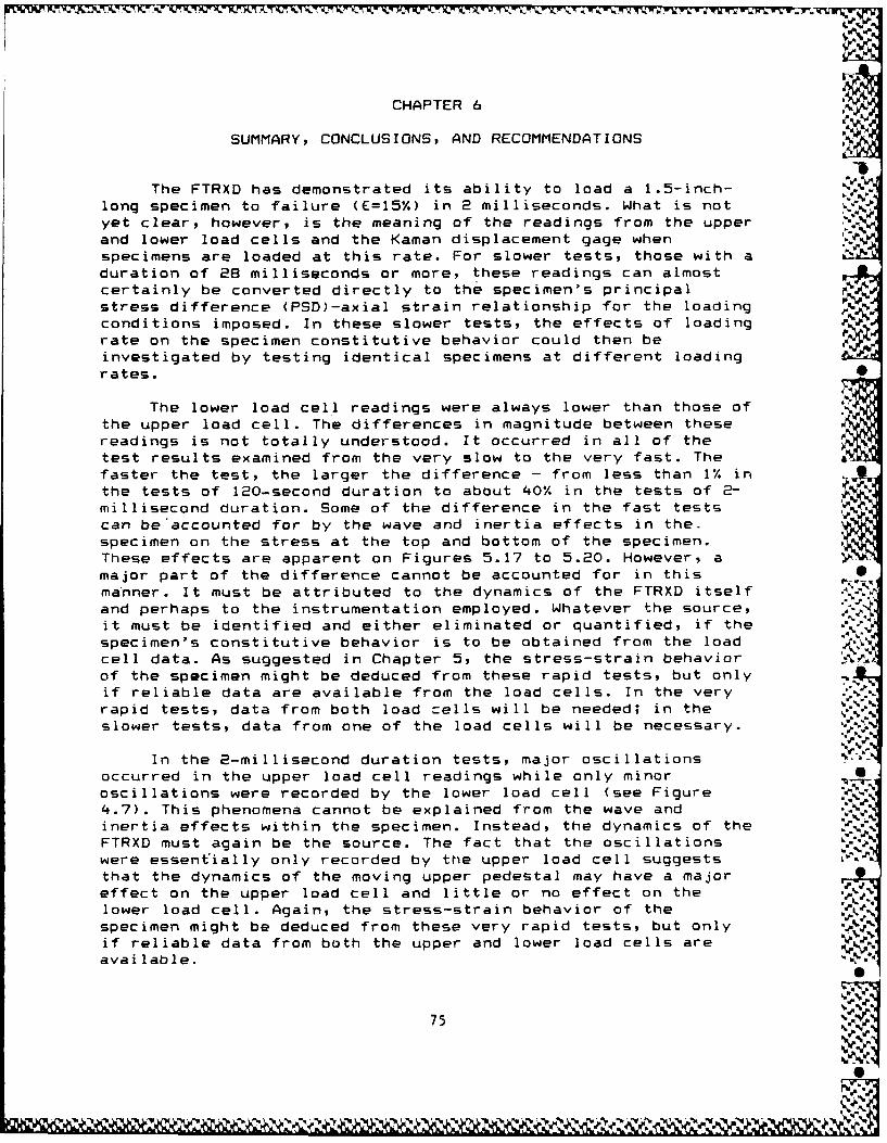
CHAPTER 6
SUMMARY, CONCLUSIONS, AND RECOMMENDATIONS
The FTRXD has demonstrated its ability to load a 1.5-inch- N.
long specimen to failure (E=15%) in 2 milliseconds. What is notyet clear, however, is the meaning of the readings from the upperand lower load cells and the Kaman displacement gage when ..4
specimens are loaded at this rate. For slower tests, those with a
duration of 28 milliseconds or more, these readings can almostcertainly be converted directly to the specimen's principalstress difference (PSD)-axial strain relationship for the loadingconditions imposed. In these slower tests, the effects of loadingrate on the specimen constitutive behavior could then beinvestigated by testing identical specimens at different loading
rates.
The lower load cell readings were always lower than those ofthe upper load cell. The differences in magnitude between thesereadings is not totally understood. It occurred in all of thetest results examined from the very slow to the very fast. The
faster the test, the larger the difference - from less than 1% inthe tests of 120-second duration to about 40% in the tests of 2-millisecond duration. Some of the difference in the fast testscan be accounted for by the wave and inertia effects in the.specimen on the stress at the top and bottom of the specimen.These effects are apparent on Figures 5.17 to 5.20. However, amajor part of the difference cannot be accounted for in this
manner. It must be attributed to the dynamics of the FTRXD itselfand perhaps to the instrumentation employed. Whatever the source,it must be identified and either eliminated or quantified, if thespecimen's constitutive behavior is to be obtained from the loadcell data. As suggested in Chapter 5, the stress-strain behaviorof the specimen might be deduced from these rapid tests, but onlyif reliable data are available from the load cells. In the veryrapid tests, data from both load =ells will be needed; in theslower tests, data from one of the load cells will be necessary.
In the 2-millisecond duration tests, major oscillationsoccurred in the upper load cell readings while only minoroscillations were recorded by the lower load cell (see Figure4.7). This phenomena cannot be explained from the wave andinertia effects within the specimen. Instead, the dynamics of theFTRXD must again be the source. The fact that the oscillationswere essentially only recorded by the upper load cell suggeststhat the dynamics of the moving upper pedestal may have a majoreffect on the upper load cell and little or no effect on thelower load cell. Again, the stress-strain behavior of thespecimen might be deduced from these very rapid tests, but onlyif reliable data from both the upper and lower load cells areavailable. ,--
75%W.
IP
-Y ~ .~ wxJ.
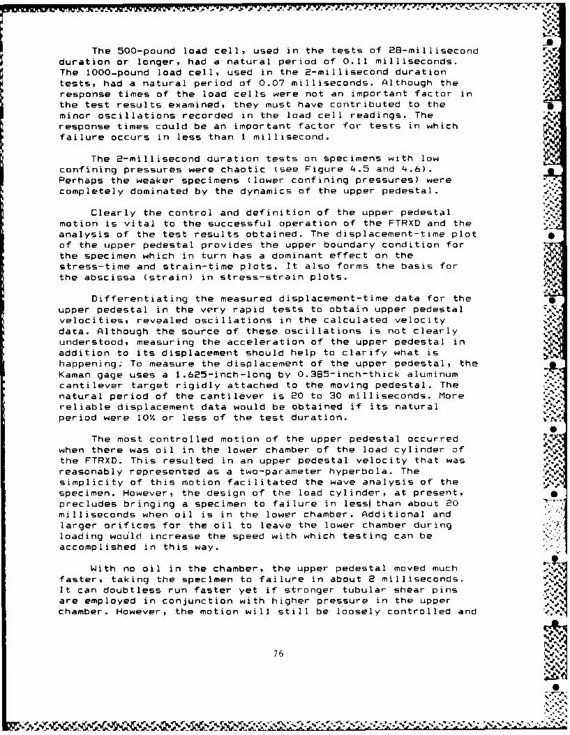
JVJ-
The 500-pound load cell, used in the tests of 28-millisecondduration or longer, had a natural period of 0.11 milliseconds.The 1000-pound load cell, used in the 2-millisecond durationtests, had a natural period of 0.07 milliseconds. Although theresponse times of the load cells were not an important factor inthe test results examined, they must have contributed to theminor oscillations recorded in the load cell readings. Theresponse times could be an important factor for tests in whichfailure occurs in less than 1 millisecond.
The 2-millisecond duration tests on specimens with lowconfining pressures were chaotic (see Figure 4.5 and 4.6).Perhaps the weaker specimens (lower confining pressures) werecompletely dominated by the dynamics of the upper pedestal.
Clearly the control and definition of the upper pedestalmotion is vital to the successful operation of the FTRXD and theanalysis of the test results obtained. The displacement-time plotof the upper pedestal provides the upper boundary condition forthe specimen which in turn has a dominant effect on thestress-time and strain-time plots. It also forms the basis forthe abscissa (strain) in stress-strain plots.
Differentiating the measured displacement-time data for theupper pedestal in the very rapid tests to obtain upper pedestal Z
velocities, revealed oscillations in the calculated velocitydata. Although the source of these oscillations is not clearlyunderstood, measuring the acceleration of the upper pedestal inaddition to its displacement should help to clarify what is
happening. To measure the displacement of the upper pedestal, theKaman gage uses a 1.625-inch-long by 0.385-inch-thick aluminumcantilever target rigidly attached to the moving pedestal. Thenatural period of the cantilever is 20 to 30 milliseconds. Morereliable displacement data would be obtained if its naturalperiod were 10% or less of the test duration.
The most controlled motion of the upper pedestal occurredwhen there was oil in the lower chamber of the load cylinder of %the FTRXD. This resulted in an upper pedestal velocity that wasreasonably represented as a two-parameter hyperbola. Thesimplicity of this motion facilitated the wave analysis of thespecimen. However, the design of the load cylinder, at present,precludes bringing a specimen to failure in lessi than about 20milliseconds when oil is in the lower chamber. Additional andlarger orifices for the oil to leave the lower chamber duringloading would increase the speed with which testing can be i".i1accomplished in this way.
With no oil in the chamber, the upper pedestal moved muchfaster, taking the specimen to failure in about 2 milliseconds.It can doubtless run faster yet if stronger tubular shear pins Iare employed in conjunction with higher pressure in the upperchamber. However, the motion will still be loosely controlled and
76 %*o

complex. It must be recorded definitively so that relevantboundary conditions for a wave analysis of the specimen can beemployed. Clearly in faster tests, the dynamics of the FTRXD willbe even more important and must be understood.
Several recommendations regarding the evaluation of theFTRXD are in order:
1. Install an accelerometer in the upper pedestal at the point ofthe Kaman gage cantilever target so that both the displacementand acceleration data of the upper pedestal may be obtained. Theaccelerometer must be able to record accelerations accurately andwithstand very large acceleration "spikes. "
2. Install a cantilever target for the Kaman gage with a naturalperiod of 0.1 milliseconds or less. The shorter and the thickerit is, the better. An aluminum cantilever of the same general 0shape as the present one but 1.25 inches thick should possess anatural period of less than 0.1 milliseconds.
3. Modify the load cylinder so that oil in its lower chamber can
be expelled faster during testing. More and symmetricallypositioned orfices of larger diameter would be desirable.Recognizing the need to open the orifices simultaneously and veryrapidly, more than one orifice may be impractical. As a minimum,the present orifice might be doubled in diameter. If simultaneity
of openings can be achieved, additional orfices will be a great
improvement.
4. Conduct a detailed examination of the load cells, their %calibration, their response times, and the manner of recordingdata from them. The purpose of this study would be to eitherverify that the difference in upper and lower load cell readings
is not caused by the load cells themselves, or if it is, toidentify and remove the source or quantify its effects. The studycould also assess the limitations of the load cells in terms of
their response times. "1
5. Conduct a detailed dynamic analysis of the FTRXD as anassemblage of deformable components possessing mass. Such an Vanalysis has been begun by the author. The FTRXD was modeled as a 9two degree of freedom system with a linear-hyperbolic masslessspring representing the soil specimen, and lumped masses andlinear springs representing the remainder of the system. Themodel shows promise, but needs refinement. Better excitation data(displacement-time or force-time) might be employed, mass mightbe added to the nonlinear spring, and the analysis might beextended to more than two degrees of freedom. The purpose of theanalysis would be to ascertain what the upper and lower loadcells should read during the very fast tests, to provide insightsinto when and how the dynamics of the upper pedestal can dominatethe effects of the soil element, and to suggest ways to improvethe FTRXD so that more usable test data may be obtained. S
77 .
-6rD-JA - - *- -

6. Conduct a series of rapid tests with the FTRXD on a wellestablished soil, such as CARES-Dry soil, prepared in specimenswhose lengths vary from 1.5 to 3 inches and whose diametersremain at 0.75 inches. The purpose of the testing would be tovalidate the modifications to the FTRXD suggested above, :o
validate better the one-dimensional wave analysis of the specimendescribed in Chapter 5, to investigate the effect of specimenstrength (confining pressure) on the dynamic response of theFTRXD, and to validate and complement the dynamic analysis of theFTRXD as recommended above.
7. Conduct a two-dimensional axisymmetric wave analysis of thespecimen initially as a linear elastic material. The purpose of .
this analysis would be to define the limits of the validity ofthe one-dimensional wave analysis. As required, it would beextended to a specimen possessing a postulated nonlinearconstitutive relationship which reflects the yielding and shearfailure anticipated in the triaxial testing of soils.
8. Conduct a series of rapid tests with the FTRXD on a variety ofsoils prepared in specimen sizes from 1.5 to 4 inches. The FTRXDwould first be modified to accomodate specimens with diameters of1.0 inch. The purpose of the testing would be to validate theanalyses of the FTRXD and to assess its utility in testing avariety of soils for their engineering properties at very rapidloading rates.
78
AL JPL Z" I.,

REFERENCES ,
1. Carroll, William F., 1963, "Vertical Displacements of SpreadFootings on Clay: Static and Impulsive Loadings," DynamicBearing Capacity of Soils, Report 5, Technical Report 3-599,US Army Engineer Waterways Experiment Station, Vicksburg, MS.
2. Cummins, Tony K., 1982, "Description of a Fast TriaxialShear Device," Draft Report to the Defense Nuclear Agency,US Army Engineer Waterways Experiment Station, Vicksburg, MS.
3. Cargile, James D., 1984, "Geotechnical Investigation for theCARES-Dry Site: Laboratory Test Results," Report to theAir Force Ballistic Missile Office/ENSN, US Army Engineer -.
Waterways Experiment Station, Vicksburg, MS. -.
4. Farr, John Vail, 1986, "Loading Rate Effects on the One- 0
Dimensional Compressibility of Four Partially SaturatedSoils, "Dissertation submitted in partial fulfillment of therequirements for the degree of Doctor of Philosophy (CivilEngineering), University of Michigan, Ann Arbor, MI.
5. Richart, F.E. jr., Hall, J.R. jr., and Woods, R.D., SVibrations of Soils and Foundations, Prentice Hall, Inc.,(Englewood Cliffs, NJ: 1970).
6. Davis, Julian, Finite-Difference Methods in Dynamics ofContinuous Media, Macmillan Publishing Co.. Inc.,(New York: 1986). -
..'.4.%.
.-
~~79 "0% -
'-P .".
*. "A

APPENDIX A
PROGRAM FTSP (FORTRAN 77)
%
% 0]
LlAl
~'% V %. %~ .~ ~ *% %'...O%. *-

C PROGRAM FTSP BY WF CARROLL, PROFESSOR, DEPT CEES, UCF
CC THIS CODE SOLVES A 1D NON-LINEAR WAVE EQUATION FOR NORMAL STRAINC AND STRESS AT THE TOP AND BOTTOM OF A TRIAXIAL SPECIMEN WHEN ITS
C UPPER PEDESTAL TRAVELS WITH A CONSTANT OR HYPERBOLIC VELOCITY ORC WITH CONSTANT ACCELERATION AND ITS STRESS-STRAIN RELATIONSHIP IS
C INITIALLY LINEAR AND THEN HYPERBOLIC.C THE SOLUTION IS A FINITE DIFFERENCE ONE.CC THE VARIABLES ARE DIMENSIONLESS:
C CTH - DIMENSIONLESS TIME (TIME TIMES INITIAL PROPAGATIONC VELOCITY (C) DIVIDED BY SPECIMEN LENGTH (H))
C CTOH - DIMENSIONLESS CHARACTERISTIC UPPER PEDESTAL TIME;C CTOH=C*TO/H WHERE TO=VO/AO:C TO - CHARACTERISTIC U.P. TIMEC VO - LIMITING U.P. VELOCITY
C AO - INITIAL U.P. ACCELERATIONC CTOH = 0 YIELDS A CONSTANT U.P. VELOCITY
C = 1000 YIELDS A CONSTANT U.P. ACCELERATIONC 1000>CTOH>O YIELDS HYPERBOLIC U.P. VELOCITIES
C CVO - C DIVIDED BY VO.C UHCVO - DISPLACEMENT DIVIDED BY H AND MULTIPLIED BY CVO.C ECVO - STRAIN MULTIPLIED BY CVO; IT ALSO INCLUDES STRESS SC DIVIDED BY THE MAX STRESS (MAX LINEAR STRESS PLUS
C MAX HYPERBOLIC STRESS).C NSS - NUMBER OF INCREMENTS IN THE SPECIMEN LENGTH (H).
C NCTH - MAX NUMBER OF TIMES THE WAVE TRAVERSES H.C AB - RATIO OF MAX HYPERBOLIC STRESS (I/B) TO INIT SLOPE (1/A)
C FOR A HYPERBOLIC STRESS-STRAIN RELATIONSHIP, AB IS A 0C CHARACTERISTIC STRAIN FOR A PURELY HYPERBOLIC MEDIUM. .
C D - AB MULTIPLIED BY CVO.C SL - MAX LINEAR DIMENSIONLESS STRESS.C EL - MAX LINEAR STRAIN.C EO - SUM OF EL AND AB, A CHARACTERISTIC STRAIN FOR AC LINEAR-HYPERBOLIC MEDIUM.
DE - EO TIMES CVO.
COMMON /CINIT/ NSSNCTH,NTS1,DCTH,CTOH,DE,D,SL,EL,CF :4.1COMMON /CU/ UHCVO(52,1052),ECVO(7,1052)
OPEN(9,FILE='FTSP.PRN',STATUS='NEW')
ALL INIT 5S DALG
.- STRAIN
F -, ,ATUS='KEEP'
., ::,'_']
I'1. -
:-1:,
'. K~l
'p.................................................-....~*,- '

SUBROUTINE INITCOMMON /CINIT/ NSS,NCTH,NTS1,DCTH,CTOH,DE,D,SL,EL,CFCOMMON /CU/ UHCVO(52,1052),ECVO(7,1052)..WRITE(*, 100)
100 FORMAT(//1X,'ENTER THE CTO/H FOR UPPER PEDESTAL MOTION'!@8X,'0 FOR CONSTANT U.P. VELOCITY, OR'/@8X11>0 FOR HYPERBOLIC U.P.VELOCITY, OR'/@BX,'1000 FOR CONSTANT U.P. ACCELERATION'//)READ(*,*) CTOHWRITE(*, 110) 5
110 FORMAT(//1X,'ENTER: THE NR OF INCREMENTS PER SPECIMEN',@1X,'LENGTH (NSI)'/@15X,'(MAX IS 50 AND MIN IS 4)'/@BX,'THE MAX EVEN INTEGER VALUE OF CT/H'!@15X,'(MAX IS 1000/NSI)'/@8X,'THE SUM OF EL AND AB (=E0) MULTIPLIED BY CVO, AND'!@8X,'THE MAX LINEAR DIMENSIONLESS STRESS (MLDS)'//)READ(*,*) NSS,NCTH,DE,SLANSS=NSSDCTH=1 ./ANSS .
NTS 1=NSS*NCTH+ 1D=DE*( 1-SL)EL=SL*DECF=1 ./(1 .+EL/D)DO 120 N=1,NTS1
* DO 120 M=1,NSS+lOHCVO(M,N)=0.
*120 CONTINUECTH=0.DO 140 N=2,NTS1
*CTH=CTH+DCTH w:
IF(CTOH .LE. .00001) THEN
GO TO 130END IFIF(CTOH .GT. 999.9 .AND. CTOH .LT. 1000.1) THENUHCVO( 1,N)=.5*CTH**2
GO TO 130END IFUHCVO( 1,N)=CTH-CTOH*ALOG( 1.+CTH/CTOH) 5'
130 ECVO(1,N)=CTHECVO(4,N)=UHCVO( 1,N)IF(ECVO(4,N) .LE. EL) ECVO(7,N)=CF*ECVO(4,N)/D p %5~
IF(ECVO(4,N) .GT. EL) THEN%ECVO(7,N)=CF*((EL/D)+(ECVO(4,N)-EL)/(D.ECVO(4,N)-EL) I
ENDIF140 CONTINUE 0
RETURN NEND
55e
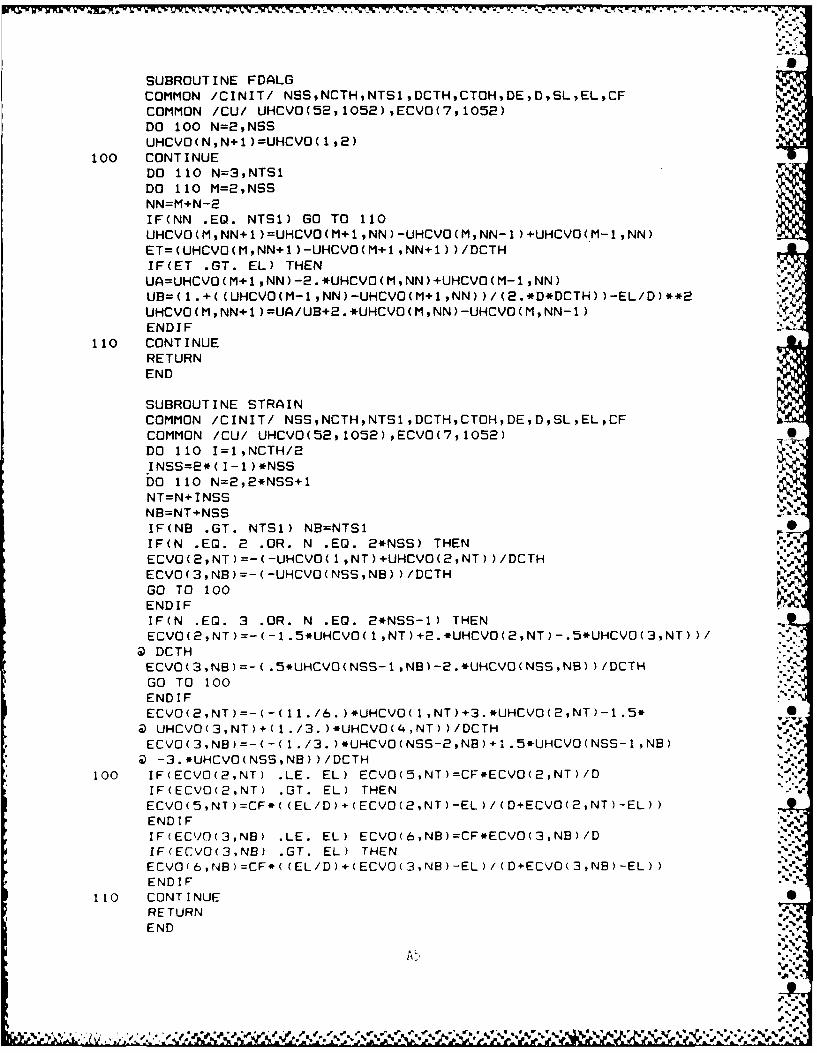
- - . . - - - K. - . t C .a . .
SUBROUTINE FDALGCOMMON /CINIT/ NSSNCTH,NTSI ,DCTH,CTOH,DE,D,SL,ELCFCOMMON /CU/ UHCVO(52,1052),ECVO(7,1052)DO 100 N=2,NSSUHCVO(N,N-1 )UHCVO( 1,2)
100 CONTINUEDO 110 N=3,NTS1DO 110 M=2,NSSNN=M+N-2IF(NN .EQ. NTS1) GO TO 110UHCVO(M,NN+1 )UHCVO(M+1 ,NN)-UHCVO(M,NN-1 )+UHCVO(.M-1 ,NN)ET=(UHCVO(MNN+1)-UHCVO(M'1,NN+1))/DCTHIF(ET .GT. EL) THENUA=UHCVO(M+1 ,NN)-2.*UHCVO(M,NN)+UHCVO(M-1 ,NN)UB=(l.4-((UHCVO(M-1,NN)-UHCVO(M+1,NN))/(2.*D*DCTH))-EL/D)**2UHCVO(M,NN.1 )=UA/UB+2.*UHCVO(M,NN)-UHCVO(M,NN-1)ENDIF
110 CONTINUERETURNEND
SUBROUTINE STRAINCOMMON /CINIT/ NSS,NCTH,NTS1,DCTHCTOH,DE,D,SL,EL,CFCOMMON /CU/ UHCVO(52,1052),ECVO(7,1052)DO 110 I=1,NCTH/2INSS=2*( I-i )*NSSDO 110 N=2,2*NSS+1NT=N+INSSNB=NT+NSS
IF(NB .GT. NTS1) NB=NTS1IF(N .EQ. 2 .OR. N .EQ. 2*NSS) THENECVO(2,NT)=-(-UHCVO(1,NT)+UHCVO(2,NT))/DCTHECVO(3,NB)=-(-UHCVO(NSS,NB))/DCTHGO TO 100ENDIFIF(N .EQ. 3 .OR. N .EQ. 2*NSS-1) THENECVO(2,NT)=-(-1.5*UHCVO(1,NT)+2.*UHCVO(2,NT)-.5*UHCVO(3,NT))/ -
@ DCTHECVO(3,NB)=-(.5*UHCVO(NSS-1,NB)-2.*UHCVO(NSS,NB))/DCTHGO TO 100END IFECVO (2, NT)=--(11 ./6. )*UHCVO (1 ,NT) +3. *UHCVO (2, NT) -1 5*@ UHCVO(3,NT)+(l./3.)*UHCVO(4,NT))/DCTHECVO(3,NB)=-(-( 1.13. )*UHCVO(NSS-2,NB)+i .5*UHCVO(NSS-1 ,NB)@ -3.*UHCVO(NSS,NB))/DCTH
100 IF(ECVO(2,NT) .LE. EL) ECVO(5,NT)=CF*ECVO(2,NT)/DIF(ECVO(2,NT) .GT. EL) THENECVO(5,NT)=CF*((EL/D)+(ECVO(2,NT)-EL)/(D+ECVO(2,NT)-EL))END IFIF(ECkJO(3,NB) .LE. EL) ECVO(6,NB)=CF*ECVO(3,NB)/DIF(ECVO(3,NB) .GT. EL) THENECVOt6,N4B)=CF*( (EL/D)+(ECVO(3,NB)-EL)/(D+ECVO(3,NB)-EL)) '
END IF
110 CONTINUERETURNEND
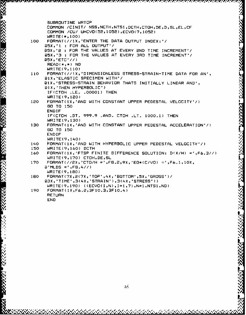
SUBROUTINE WRTOPCOMMON /CINIT/ NSSNCTHNTS1,DCTH,CTOHDED,SL,EL,CFCOMMON /CU/ UHCVO(52,1052),ECVO(7,1052)WRITE(*,100)
100 FORMAT(//IX,'ENTER THE DATA OUTPUT INDEX:'/
@5X,'1 : FOR ALL OUTPUT'/@5X,'2 : FOR THE VALUES AT EVERY 2ND TIME INCREMENT'/
@5X,'3 : FOR THE VALUES AT EVERY 3RD TIME INCREMENT'/@5X,'ETC'//)
READ(*,*) NDWRITE(9,110)
110 FORMAT(//!X,'DIMENSIONLESS STRESS-STRAIN-TIME DATA FOR AN',@IX,'ELASTIC SPECIMEN WITH'/@lX,'STRESS-STRAIN BEHAVIOR THATS INITIALLY LINEAR AND',@IX,'THEN HYPERBOLIC')IF(CTOH .LE. .00001) THENWRITE(9,120)
120 FORMAT(1X,'AND WITH CONSTANT UPPER PEDESTAL VELOCITY'/)GO TO 150
ENDIFIF(CTOH .GT. 999.9 .AND. CTOH .LT. 1000.1) THENWRITE(9,130)
130 FORMAT(1X,'AND WITH CONSTANT UPPER PEDESTAL ACCELERATION'/)GO TO 150
ENDIFWRITE(9,140)
140 FORMAT(1X,'AND WITH HYPERBOLIC UPPER PEDESTAL VELOCITY'/)150 WRITE(9,160) DCTH160 FORMAT(1X,'FTSP FINITE DIFFERENCE SOLUTION: D(X/H) =',F6.3//)
WRITE(9,170) CTOH,DE,SL170 FORMAT(//2X,'CTO/H =',F8.2,9X,'EO*(C/VO) =',F6.1,1OX,
@ 'MLDS =',F8.4//)
WRITE(9,180)
180 FORMAT(7X,2(7X,'TOP',4X,'BOTTOM',5X,'GROSS')/
@3X,'TIME',3(4X,'STRAIN'),3(4X,'STRESS'))WRITE(9,190) ((ECVO(I,N),I=1,7),N=1,NTS1,ND)
190 FORMAT(1X,F6.2,3FI0.3,3FI0.4)RETURN
END
%40
A6S

APPENDIX B
SAMPLE DATA RUN FROM
PROGRAM FTSP (FORTRAN 77)
Hyperbolic Upper Pedestal Motion,
C t /h = 5.00 0
Linear-Hyperbolic Stress-Strain, .
q T max = MLDS = 0.25 A9
E = 10.0
N
0
.B11
4 1%

DIMENSIONLESS STRESS-STRAIN-TIME DATA FOR AN ELASTIC SPECIMEN WITH
STRESS-STRAIN BEHAVIOR THATS INITIALLY LINEAR AND THEN HYPERBOLIC
AND WITH HYPERBOLIC UPPER PEDESTAL VELOCITY
FTSP FINITE DIFFERENCE SOLUTION: D(X/H) = 0.050
CTO/H = 5.00 EO*(C/VO) = 10.0 MLDS = 0.2500
TOP BOTTOM GROSS TOP BOTTOM GROSS 0 ,
TIME STRAIN STRAIN STRAIN STRESS STRESS STRESS
0.00 0.000 0.000 0.000 0.0000 0.0000 0.00000.20 0.038 0.000 0.004 0.0038 0.0000 0.0004
0.40 0.074 0.000 0.015 0.0074 0.0000 0.0015
0.60 0.107 0.000 0.033 0.0107 0.0000 0.0033 S
0.80 0.138 0.000 0.058 0.0138 0.0000 0.0058
1.00 0.167 0.000 0.088 0.0167 0.0000 0.008
1.20 0.194 0.077 0.124 0.0194 0.0077 0.0124
1.40 0.219 0.148 0.166 0.0219 0.0148 0.0166
1.60 0.242 0.214 0.212 0.0242 0.0214 0.0212
1.80 0.265 0.276 0.263 0.0265 0.0276 0.0263 0
2.00 0.286 0.333 0.318 0.0286 0.0333 0.0318
2.20 0.382 0.387 0.377 0.0382 0.0387 0.0377
2.40 0.472 0.437 0.440 0.0472 0.0437 0.0440 . .,
2.60 0.556 0.485 0.506 0.0556 0.0485 0.0506
2.80 0.635 0.529 0.577 0.0635 0.0529 0.0577
3.00 0.708 0.571 0.650 0.0708 0.0571 0.0650
3.20 0.777 0.688 0.727 0.0777 0.0688 0.0727
3.40 0.842 0.797 0.806 0.0642 0.0797 0.0806
3.60 0.903 0.898 0.66 0.0903 0.0898 0.0888o~o .3.80 0.961 0.994 0.973 0.0961 0.0994 0.0973
4.00 1.016 1.083 1.061 0.1016 0.1083 0.1061
4.20 1.145 1.168 1.151 0.1145 0.1168 0.1151
4.40 1.265 1.247 1.244 0.1265 0.1247 0.1244
4.60 1.378 1.322 1.338 0.1378 0.1322 0.1338
4.80 1.484 1.393 1.435 0.1464 0.1393 0.1435
5.00 1.583 1.460 1.534 0.1583 0.1460 0.1534
5.20 1.677 1.601 1.635 0.1677 0.1601 0.1635
5.40 1.766 1.733 1.738 0.1766 0.1733 0.1738
5.60 1.850 1.857 1.843 0.1850 0.1857 0.1843
5.80 1.930 1.973 1.949 0.1930 0.1973 0,1949
6.00 2.006 2.083 2.058 0.2006 0.2083 0.2058
6.20 2.155 2.187 2.168 0.2155 0.2187 0.2168
6.40 2.294 2.285 2.279 0.2294 0.2285 0.2279
6.60 2.426 2.379 2.392 0.2426 0.2379 0.2392
6.80 2.550 2.467 2.507 0.2549 0.2467 0.2507
7.00 2.667 2.551 2.623 0.2663 0.2551 0.2621
7.20 2.778 2.708 2.740 0.2768 0.2702 0.2733 V.
7.40 2.884 2.854 2.859 0.2866 0.2838 0.2842
7.60 2.985 2.993 2.979 0.2956 0.2963 0.2950
B3
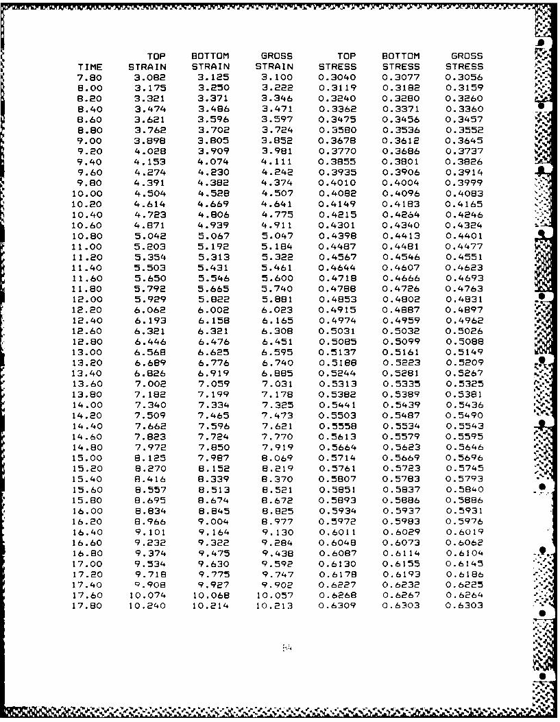
TOP BOTTOM GROSS TOP BOTTOM GROSS
TIME STRAIN STRAIN STRAIN STRESS STRESS STRESS7.80 3.082 3.125 3.100 0.3040 0.3077 0.30568.00 3.175 3.250 3.222 0.3119 0.3182 0.31598.20 3.321 3.371 3.346 0.3240 0.3280 0.3260
8.40 3.474 3.486 3.471 0.3362 0.3371 0.33606.60 3.621 3.596 3.597 0.3475 0.3456 0.3457
8.80 3.762 3.702 3.724 0.3580 0.3536 0.35529.00 3.898 3.805 3.852 0.3678 0.3612 0.3645
9.20 4.028 3.909 3.961 0.3770 0.3686 0.37379.40 4.153 4.074 4.111 0.3855 0.3801 0.3826
9.60 4.274 4.230 4.242 0.3935 0.3906 0.39149.80 4.391 4.382 4.374 0.4010 0.4004 0.3999
10.00 4.504 4.528 4.507 0.4082 0.4096 0.4083
10.20 4.614 4.669 4.641 0.4149 0.4183 0.416510.40 4.723 4.806 4.775 0.4215 0.4264 0.4246
10.60 4.871 4.939 4.911 0.4301 0.4340 0.432410.80 5.042 5.067 5.047 0.4398 0.4413 0.4401
11.00 5.203 5.192 5.184 0.4487 0.4481 0.447711.20 5.354 5.313 5.322 0.4567 0.4546 0.455111.40 5.503 5.431 5.461 0.4644 0.4607 0.462311.60 5.650 5.546 5.600 0.4718 0.4666 0.469311.80 5.792 5.665 5.740 0.4768 0.4726 0.4763
12.00 5.929 5.822 5.881 0.4853 0.4802 0.483112.20 6.062 6.002 6.023 0.4915 0.4887 0.489712.40 6.193 6.158 6.165 0.4974 0.4959 0.496212.60 6.321 6.321 6.308 0.5031 0.5032 0.502612.80 6.446 6.476 6.451 0.5085 0.5099 0.5088
13.00 6.568 6.625 6.595 0.5137 0.5161 0.5149
13.20 6.689 6.776 6.740 0.5188 0.5223 0.520913.40 6.826 6.919 6.8B5 0.5244 0.5281 0.5267
13.60 7.002 7.059 7.031 0.5313 0.5335 0.532513.80 7.182 7.199 7.178 0.5382 0.5389 0.5381
14.00 7.340 7.334 7.325 0.5441 0.5439 0.5436 PIP14.20 7.509 7.465 7.473 0.5503 0.5487 0.5490
14.40 7.662 7.596 7.621 0.5558 0.5534 0.554314.60 7.823 7.724 7.770 0.5613 0.5579 0.559514.80 7.972 7.850 7.919 0.5664 0.5623 0.5646
15.00 8.125 7.987 8.069 0.5714 0.5669 0.5696 .1%15.20 8.270 8.152 8.219 0.5761 0.5723 0.574515.40 8.416 8.339 8.370 0.5807 0.5783 0.5793
15.60 8.557 8.513 8.521 0.5851 0.5837 0.5840 •15.80 8.695 8.674 6.672 0.5893 0.5886 0.5886
16.00 8.834 8.845 8.825 0.5934 0.5937 0.593116.20 8.966 9.004 8.977 0.5972 0.5983 0.5976
16.40 9.101 9.164 9.130 0.6011 0.6029 0.601916.60 9.232 9.322 9.284 0.6048 0.6073 0.606216.80 9.374 9.475 9.438 0.6087 0.6114 0.6104 -17.00 9.534 9.630 9.592 0.6130 0.6155 0.614517.20 9.718 9.775 9.747 0.6178 0.6193 0.618617.40 9.908 9.927 9.902 0.6227 0.6232 0.622517.60 10.074 10.068 10.057 0.6268 0.6267 0.6264
17.80 10.240 10.214 10.213 0.6309 0.6303 0.6303
%
%1~
.6.'

;%- .{ - - - a .. . . . .,..-. . .. -.... b :. _ - -, - .
ATOP BOTTOM GROSS TOP BOTTOM GROSS
TIME STRAIN STRAIN STRAIN STRESS STRESS STRESS18.00 10.413 10.352 10.370 0.6351 0.6336 0.634018.20 10.579 10.493 10.526 0.6389 0.6369 0.637718.40 10.737 10.629 10.684 0.6426 0.6401 0.641318.60 10.903 10.769 10.841 0.6463 0.6433 0.644918.80 11.060 10.912 10.999 0.6497 0.6465 0.648419.00 11.214 11.073 11.157 0.6531 0.6500 0.651919.20 11.373 11.251 11.315 0.6564 0.6539 0.655219.40 11.521 11.444 11.474 0.6595 0.6579 0.658619.60 11.674 11.627 11.633 0.6627 0.6617 0.661819.80 11.822 11.797 11.793 0.6656 0.6651 0.665020.00 11.967 11.962 11.953 0.6685 0.6684 0.668220.20 12.114 12.139 12.113 0.6713 0.6718 0.671320.40 12.256 12.310 12.273 0.6740 0.6750 0.674420.60 12.399 12.471 12.434 0.6767 0.6780 0.677420.80 12.543 12.635 12.595 0.6794 0.6810 0.680321.00 12.688 12.802 12.757 0.6820 0.6840 0.683221.20 12.849 12.961 12.918 0.6849 0.6868 0.686121.40 13.020 13.116 13.080 0.6878 0.6895 0.688921.60 13.212 13.280 13.243 0.6911 0.6923 0.691721.80 13.403 13.431 13.405 0.6943 0.6948 0.694422.00 13.589 13.585 13.568 0.6974 0.6973 0.697122.20 13.759 13.739 13.731 0.7002 0.6998 0.699722.40 13.927 13.889 13.894 0.7028 0.7022 0.702322.60 14.103 14.035 14.058 0.7055 0.7045 0.704822.80 14.280 14.187 14.222 0.7082 0.7068 0.707423.00 14.451 14.332 14.386 0.7108 0.7090 0.709823.20 14.613 14.478 14.551 0.7132 0.7112 0.712323.40 14.779 14.631 14.715 0.7156 0.7135 0.714723.60 14.951 14.784 14.880 0.7181 0.7157 0.717123.80 15.112 14.951 15.045 0.7203 0.7181 0.719424.00 15.271 15.133 15.211 0.7225 0.7206 0.721724.20 15.432 15.322 15.376 0.7247 0.7232 0.723924.40 15.594 15.518 15.542 0.7269 0.7258 0.726224.60 15.751 15.707 15.708 0.7289 0.7284 0.728424.80 15.903 15.882 15.875 0.7309 0.7306 0.730525.00 16.062 16.055 16.041 0.7329 0.7328 0.732725.20 16.217 16.227 16.208 0.7349 0.7350 0.734825.40 16.363 16.403 16.375 0.7367 0.7372 0.736825.60 16.518 16.585 16.542 0.7386 0.7394 0.738925.80 16.671 16.758 16.710 0.7404 0.7415 0.740926.00 16.820 16.922 16.877 0.7422 0.7434 0.7429 o26.20 16.975 17.090 17.045 0.7440 0.7454 0.744826.40 17.136 17.261 17.213 0.7459 0.7473 0.746826.60 17.305 17.430 17.381 0.7478 0.7492 0.748726.80 17.482 17.597 17.550 0.7498 0.7511 0.7506 A27.00 17.672 17.755 17.718 0.7519 0.7528 0.752427.20 17.870 17.918 17.887 0.7540 0.7546 0.754227.40 18.063 18.085 18.056 0.7561 0.7563 0.756027.60 18.250 18.245 18.226 0.7581 0.7580 0.757827.80 18.433 18.401 18.395 0.7600 0. 759eo 0.7596 1
28.00 18.604 18.559 18.565 0.7617 0.7612 0.7613@

TOP BOTTOM GROSS TOP BOTTOM GROSSTIME STRAIN STRAIN STRAIN STRESS STRESS STRESS
28.20 18.775 16.718 18.734 0.7634 0.7628 0.763028.40 18.957 16.876 18.904 0.7652 0.7644 0.764728.60 19.137 19.028 19.074 0.7670 0.7659 0.7663 -26.80 19.316 19.181 19.245 0.7687 0.7674 0.768029.00 19.492 19.340 19.415 0.7703 0.7689 0.7696
29.20 19.659 19.499 19.586 0.7719 0.7704 0.771229.40 19.826 19.655 19.757 0.7734 0.7719 0.772829.60 19.998 19.820 19.928 0.7750 0.7734 0.774329.80 20.174 19.999 20.099 0.7766 0.7750 0.775930.00 20.346 20.180 20.270 0.7781 0.7766 0.777430.20 20.505 20.365 20.442 0.7795 0.7782 0.778930.40 20.670 20.564 20.613 0.7809 0.7800 0.780430.60 20.839 20.763 20.785 0.7823 0.7617 0.781930.80 21.001 20.954 20.957 0.7837 0.7833 0.783331.00 21.169 21.141 21.129 0.7851 0.7848 0.784731.20 21.332 21.320 21.302 0.7864 0.7863 0.786131.40 21.485 21.496 21.474 0.7876 0.7877 0.787531.60 21.647 21.673 21.647 0.7889 0.7891 0.788931.80 21.813 21.848 21.820 0.7902 0.7905 0.790332.00 21.969 22.029 21.992 0.7914 0.7919 0.791632.20 22.125 22.217 22.165 0.7926 0.7933 0.792932.40 22.284 22.397 22.339 0.7938 0.7947 0.794232.60 22.446 22.569 22.512 0.7951 0.7960 0.795532.80 22.611 22.739 22.685 0.7963 0.7972 0.796833.00 22.775 22.909 22.859 0.7975 0.7985 -0.798133.20 22.943 23.083 23.033 0.7987 0.7997 0.799333.40 23.122 23.258 23.207 0.8000 0.8009 0.800633.60 23.311 23.431 23.381 0.8013 0.8022 0.801833.80 23.502 23.605 23.555 0.8026 0.8034 0.803034.00 23.697 23.771 23.729 0.8040 0.8045 0.804234.20 23.893 23.932 23.904 0.8053 0.8056 0.8054 -W34.40 24.090 24.100 24.078 0.8066 0.8067 0.806634.60 24.266 24.274 24.253 0.8079 0.8078 0.807734.80 24.472 24.440 24.428 0.8091 0.8089 0.808935.00 24.648 24.602 24.603 0.8103 0.8100 0.810035.20 24.825 24.766 24.778 0.8114 0.8110 0.811135.40 25.005 24.926 24.953 0.8125 0.8120 0.812235.60 25.186 25.089 25.128 0.8137 0.8131 0.813335.80 25.366 25.254 25.304 0.8148 0.8141 0.814436.00 25.549 25.419 25.479 0.8159 0.8151 0.815436.20 25.735 25.581 25.655 0.8170 0.8161 0.816536.40 25.919 25.740 25.831 0.8181 0.8170 0.817636.60 26.096 25.902 26.006 0.8191 0.8180 0.818636.80 26.266 26.071 26.182 0.8201 0.8190 0.819637.00 26.435 26.248 26.359 0.8211 0.8200 0.820637.20 26.609 26.423 26.535 0.8220 0.8210 0.821637.40 26.788 26.596 26.711 0.8230 0.8220 0.822637.60 26.966 26.780 26.888 0.8240 0.8230 0.823637.80 27.141 26.978 27.064 0.8250 0.8241 0.824638.00 27.313 27.177 27.241 0.8259 0.8252 0.825538.20 27.482 27.372 27.418 0.8268 0.8262 0.8265
B6
I l
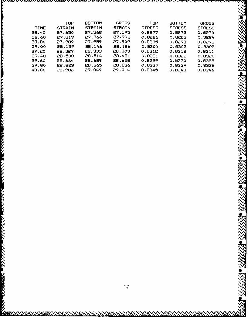
TOP BOTTOM GROSS TOP BOTTOM GROSSTIME STRAIN STRAIN STRAIN STRESS STRESS STRESS
38.40 27.650 27.568 27.595 0.8277 0.6273 0.827438.60 27.819 27.766 27.772 0.8286 0.6283 0.628436.80 27.969 27.959 27.949 0.6295 0.8293 0.829339.00 28.159 28.146 26.126 0.8304 0.6303 0.830239.20 26.329 28.333 28.303 0.8312 0.6312 0.831139.40 26.500 26.514 28.461 0.8321 0.8322 0.832039.60 28.664 26.669 26.658 0.6329 0.8330 0.632939.80 26.623 28.665 26.636 0.8337 0.8339 0.833640.00 26.986 29.049 29.014 0.8345 0.8346 0.8346
1p
N
DISTRIBUTION LIST
DEPARTMENT OF DEFENSE Commander/DirectorUS Army Cold Regions Research and
Director Engineering LaboratoryDefense Nuclear Agency ATTN: Technical LibraryATTN: DFSP (Dr. G. W. Ullrich) 72 Lyme Road
SPSD (MAJ M. A. Reed) Hanover, NH 03755-1290SPWE (Dr. C. Canada)SPWE (MAJ M. Pelkey) CommandantTechnical Library US Army Engineer School
Washington, DC 20305-1000 ATTN: ATZA-CD (COL Fred Parker) "VTechnical Library
Defense Nuclear Agency Ft. Belvoir, VA 22060-5281Nevada Operations OfficeATTN: TDNV (Mr. J. W. LaComb) Commander .P. 0. Box 208 US Army Laboratory CommandMercury, NV 89023 ATTN: Technical Library %
2800 Powder Mill Road .-
Director Adelphi, MD 20783-1145 %Defense Advanced Research Project AgencyATTN: Technical Library Director S1400 Wilson Blvd. US Army Ballistic Research LaboratoryArlington, VA 22209 ATTN: Technical Library
Aberdeen Proving Ground, MD 21005-5066DirectorDefense Intelligence Agency CommanderATTN: Technical Library US Army Nuclear and Chemical AgencyWashington, DC 20301-6111 ATTN: Technical Library
7500 Backlick Road, Bldg. 2073Defense Technical Information Center Springfield, VA 22150Cameron StationATTN: TC (2"cys)Alexandria, VA 22314 DEPARTMENT OF THE NAVY
Naval Civil Engineering LaboratoryDEPARTMENT OF THE ARMY ATTN: Technical Library
Port Hueneme, CA 93043CommanderUS Army Corps of Engineers Naval Facilities Engineering CommandATTN: CERD-L (Ms. Sharon Vannucci) ATTN: Technical Library
CERD-M (Mr. B. 0. Benn) 200 Stovall Street %.CEEC-ET (Mr. R. L. Wight) Alexandria, VA 22332CEIM-SL
Washington, DC 20314-1000DEPARTMENT OF THE AIR FORCE
Division EngineerUS Army Engineer Division, Huntsville Air Force Institute of TechnologyATTN: CEHND-SR Air UniversityP. 0. Box 1600, West Station ATTN: Technical LibraryHuntsville, AL 35807-4301 Wright-Patterson Air Force Base, OH .53 3
District Engineer Air Force Office of Scientific ResearchUS Army Engineer District, Omaha ATTN: Technical LibraryATTN: CEMRO-ED-S (Mr. Bob Kelley) Bolling Air Force Base, DC 20332
CEMPO-ED-SH (Mr. Bill Gaube)215 N. 17th Street Air Force Weapons Laboratory (AFSC)%%3maha, NE 68102-4978 ATTN: NTESG (CPT C. W. Felice)
Technical LibraryDirector Kirtland Air Force Base, NM''S Army Construction Engineerlng
Research Laboratory Air Force Engineering an Ce-vi-esATTN: Technical Library Center (AF2P. O. Box 305 ATTN: Technicai '.ibrarv -".3Cnampaign, 1'- 61820-1305 Tyndall Air Force Base. F_ 32"03 '%
Air Force Armament Latoratory 'AFCS'ATTN: Technical Library VEglin Air Force Basp, FL 325-
-O.'

DISTRIBUTION LIST (CONTINUED)
DEPARTMENT OF THE AIR FORCE (Continued) Dr. K. C. ValanisEndochronics, Inc.
Commander 8605 Northwest Lakecrest CourtBallistic Missile Office (AFSC) Vancouver, WA 98665ATTN: MYEB (LTC D. H. Gage)
Technical Library Technical LibraryNorton Air Force Base, CA 92409 New Mexico Engineering Research Institute
University of New MexicoBox 25, University Station
DEPARTMENT OF ENERGY Albuquerque, NM 87131
Lawrence Livermore National Laboratory Dr. Don SimonsATTN: Technical Library R&D AssociatesP. 0. Box 808 P. 0. Box 9695Livermore, CA 94550 Marina del Rey, CA 90291
Los Alamos National Laboratory Mr. L. S. MelzerATTN: Technical Library Science Applications InternationalP. 0. Box 1663 CorporationLos Alamos, NM 87545 505 West Texas Street
First City Center, Tower 2, Suite 1335Sandia National Laboratories Midland, TX 79701ATTN: Technical LibraryP. 0. Box 5800 Dr. John SchatzAlbuquerque, NM 87185 Science Applications International
CorporationSandia National Laboratories P. 0. Box 2351ATTN: Technical Library La Jolla, CA 92038-2351Livermore, CA 94550
Dr. H. E. ReadS-Cubed
DEPARTMENT OF DEFENSE CONTRACTORS P. 0. Box 1620La Jolla, CA 92038-1620
Mr. J. L. BrattonApplied Research Associates, Inc. Dr. Lynn Seaman
4300 San Mateo Blvd., NE, Suite A220 SRI InternationalAlbuquerque, NM 87110 333 Ravenswood Avenue
Menlo Park, CA 94025Mr. J. D. Shinn"-'
Applied Research Associates, Inc. Mr. S. J. GreenSouth Royalton, VT 05068 Terra Tek, Inc.
420 Wakara WayMr. J. L. Drake Salt Lake City, UT 8410,Applied Research Associates, Inc.3202 Wisconsin Avenue Dr. M. G. Katona ..
Vicksburg, MS 39180-2610 TRW Defense Systems 3roupP. 0. Box 1310 ..
Dr. J. G. Trulio San Bernardino, CA 92 02Applied Theory, Inc.930 S. Labrea Avenue Dr. I. S. SandlerLos Angeles, CA 90036 Weidlinger Associates
333 Seventh AvenueDr. Y. Marvin Ito New York, NY 10001California Research & Technology, Inc.20943 Devonshire Street Dr. W. F. Carroll (10 cvs' *
Chatsworth, CA 91311-2376 Department of Civil Engineeringand Environment3l ,-c-ences
Dr. E. J. Rinohart University of Central FlgrldaCalifornia Research & Technology, Inc. Orlando, FL 328162017 Yale Blvd., SEAlbuquerque, NM 87106
Dr. Hon-Yim Ko '-""
Department of Civil, Environmental, andArohItectural Engineering
University of Colorado at BoulderBoulder, CO 80309

.
I i.. .
, -'. '
-A %"~
i ,.-..V
/ *
- V -:.N: :.-'