Evaluation of Stereo Vision Obstacle Detection Algorithms for Off-Road Autonomous Navigation

Arturo Rankin1, Andres Huertas, and Larry Matthies

Jet Propulsion Laboratory, Pasadena, CA, 91109

ABSTRACT

Reliable detection of non-traversable hazards is a key requirement for off-road autonomous navigation. Under the Army Research Laboratory (ARL) Collaborative Technology Alliances (CTA) program, JPL has evaluated the performance of seven obstacle detection algorithms on a General Dynamics Robotic Systems (GDRS) surveyed obstacle course containing 21 obstacles. Stereo imagery was collected from a GDRS instrumented train traveling at 1m/s, and processed off-line with run-time passive perception software that includes: a positive obstacle detector, a negative obstacle detector, a non-traversable tree trunk detector, an excessive slope detector, a range density based obstacle detector, a multi-cue water detector, and a low-overhang detector. On the 170m course, 20 of the 21 obstacles were detected, there was complementary detection of several obstacles by multiple detectors, and there were no false obstacle detections. A detailed description of each obstacle detection algorithm and their performance on the surveyed obstacle course is presented in this paper.

Keywords: Stereo vision, passive perception, obstacle detection, autonomous navigation, geometric reasoning

1. INTRODUCTION

The ability to detect and avoid driving hazards is critical for autonomous navigation of

unmanned ground vehicles. There are two primary ways to detect driving hazards. With

discrete obstacle detection, regions in a range image or terrain map are labeled as either

traversable or nontraversable. Alternatively, the cells in a terrain map can be analyzed and

assigned a traversability cost [7]. Cells containing no hazards, mild hazards, or severe hazards

would be assigned low, mid, and high traversability costs, respectively. In uncluttered

environments, however, where the non-obstacle terrain is equally traversable, discrete obstacle

detection is sufficient.

1 Arturo.Rankin@jpl.nasa.gov, phone: (818) 354-9269, fax: (818) 393-4085, http://robotics.jpl.nasa.gov/~arankin

While some discrete obstacle detection methods assume that obstacles lie on a flat ground

plane [11,13], others allow for undulated terrain [1,3,5]. Some methods fit a planar surface to a

patch of points [4]. Other methods measure 3D slopes and the height of visible patches of terrain

[8,12]. It is difficult, however, to detect all types of discrete obstacles with a single approach.

Here, we examine a multi-algorithm approach to discrete obstacle detection.

To evaluate the performance of discrete obstacle detection, GDRS constructed an

obstacle detection test course consisting of an instrumented train, ~170m of train track, and 21

pre-surveyed obstacles. The test course was designed to enable the evaluation of multiple

contractor perception systems under identical conditions. JPL performed a stereo data collection

on the test course on June 2, 2004. Train state tagged wide (30cm), mid (20.5cm), and narrow

baseline (9.5cm) stereo imagery was collected at train speeds of 1, 3, and 5m/s. Seven discrete

obstacle detection algorithms were then implemented to detect the discrete obstacles on the

course, where each algorithm targets specific terrain characteristics. This paper describes the

seven obstacle detection algorithms and provides some results on how each performed at a train

speed of 1m/s when wide baseline stereo imagery is processed at a resolution of 320x240.

2. HARDWARE DESCRIPTION

The GDRS instrumented train is driven using a General Electric 24 volt DC motor and an

Ogura Fail-Safe brake. The train utilizes the same autonomous mobility computing hardware

used on GDRS experimental unmanned vehicles (XUVs). Data from an inertial measurement

unit (IMU) and differential global positioning system (DGPS) is combined with a Kalman filter

to provide absolute positioning accurate to within 0.5% of distance traveled when the train is

started from a surveyed start position. Power is provided by 12 volt DC batteries and an onboard

gas generator. A platform is provided above the train chassis to mount perception sensors.

The JPL passive perception system consisted of three Hitachi HV-C20 3CCD color

cameras mounted to a camera bar, one VAC VB/BBG-3 sync generator, and one portable VME

computer backplane, containing one Synergy MicroSystems VSS4 single board computer, one

Red Rock Technologies 120GB SCSI disk, and two Active Silicon SNP-PMC-24 analog

framegrabbers. The camera bar was mounted to the train’s top mounting platform with shims

that provided a 10º down tilt. Figure 1 shows a picture of the JPL passive perception system

mounted to the GDRS instrumented train.

Cameras Computer

Figure 1. A JPL passive perception system was mounted to the GDRS instrumented train.

3. SURVEYED OBSTACLE COURSE DESCRIPTION

The site selected for the obstacle detection course consisted of open level terrain with tall

grass to the left side of the train track and freshly mowed (short) grass to the right side of the

train track. The train track contained three straight sections of 45 meters each and two curved

sections having a curvature of 1/(23.25m). Objects were positioned to the sides of the train track

and surveyed by GDRS using DPGS. The obstacle course contained two small man-made water

bodies, three large dirt mounds, three tree trunks, stacked cement blocks one, two and three high,

an “L” shaped trench parallel to the tracks, a vertical 4”x4” post, vertical PVC pipes, and two

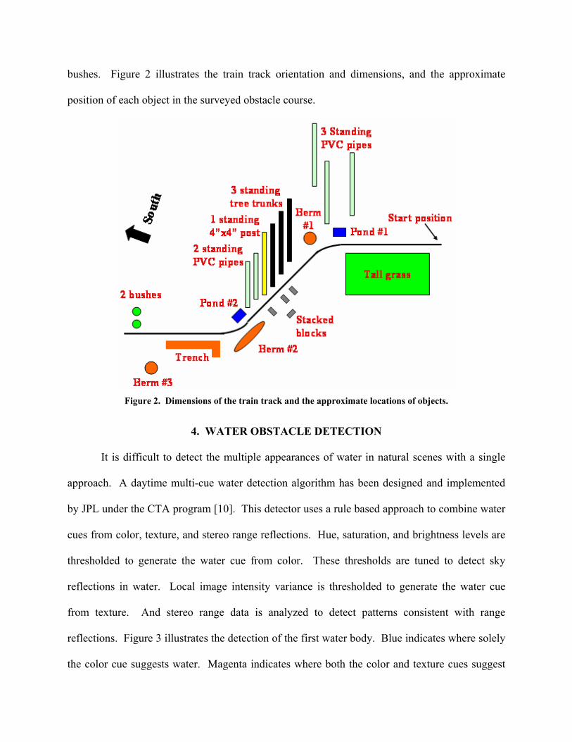
bushes. Figure 2 illustrates the train track orientation and dimensions, and the approximate

position of each object in the surveyed obstacle course.

Figure 2. Dimensions of the train track and the approximate locations of objects.

4. WATER OBSTACLE DETECTION

It is difficult to detect the multiple appearances of water in natural scenes with a single

approach. A daytime multi-cue water detection algorithm has been designed and implemented

by JPL under the CTA program [10]. This detector uses a rule based approach to combine water

cues from color, texture, and stereo range reflections. Hue, saturation, and brightness levels are

thresholded to generate the water cue from color. These thresholds are tuned to detect sky

reflections in water. Local image intensity variance is thresholded to generate the water cue

from texture. And stereo range data is analyzed to detect patterns consistent with range

reflections. Figure 3 illustrates the detection of the first water body. Blue indicates where solely

the color cue suggests water. Magenta indicates where both the color and texture cues suggest

water. And red indicates where the color, texture, and stereo range cues suggest water. Water is

reported only in regions where two or more water cues overlap. Note that there is range data on

the reflection of the white PVC pipe in the water body, enabling it to be detected by the stereo

range reflection detector.

Figure 3. A frame showing the first man-made water body (left), a 320x240 stereo range image (middle), and water detection results overlaid on an intensity image (right).

5. TREE TRUNK OBSTACLE DETECTION

A non-traversable tree trunk obstacle detector was developed by JPL under the Defense

Advanced Research Projects Agency (DARPA) Perception for Off-Road Robots (PerceptOR)

program [6,9]. It was developed for autonomous navigation in forested areas that contain a

mixture of densely distributed thin and thick trees. To make progress there, an unmanned

ground vehicle (UGV) must decide which trees it can push over and which trees it must

circumnavigate. Although it is referred to as a tree trunk detector, it is designed to detect any tall

thin vertical structure. The surveyed obstacle course contained vertically positioned PVC pipes,

tree trunks, and a 4”x4” post. We rely primarily on the tree trunk obstacle detector to detect

these items.

Edge detection assists the process. A first derivative Gaussian convolution is first applied

to an intensity image in the horizontal direction to extract long and vertical edges. A contour

extraction step then matches anti-parallel line pairs that correspond to the edges of individual

trees. Stereo ranging is performed and the minimum range within each trunk fragment is

recorded. The diameters of each tree is then estimated, based on the minimum range to the tree,

the focal length of the camera, and the distance in pixels between matched contour lines. We

threshold the estimated tree diameter and the angle of each tree fragment in the image plane (to

limit detection to near-vertical structure). In addition, we threshold the 3D tree fragment height

and stand angle to avoid detecting vertical objects in the image plane that in 3D are lying on the

ground (such as the train tracks).

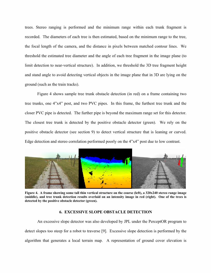
Figure 4 shows sample tree trunk obstacle detection (in red) on a frame containing two

tree trunks, one 4”x4” post, and two PVC pipes. In this frame, the furthest tree trunk and the

closer PVC pipe is detected. The further pipe is beyond the maximum range set for this detector.

The closest tree trunk is detected by the positive obstacle detector (green). We rely on the

positive obstacle detector (see section 9) to detect vertical structure that is leaning or curved.

Edge detection and stereo correlation performed poorly on the 4”x4” post due to low contrast.

Figure 4. A frame showing some tall thin vertical structure on the course (left), a 320x240 stereo range image (middle), and tree trunk detection results overlaid on an intensity image in red (right). One of the trees is detected by the positive obstacle detector (green).

6. EXCESSIVE SLOPE OBSTACLE DETECTION

An excessive slope detector was also developed by JPL under the PerceptOR program to

detect slopes too steep for a robot to traverse [9]. Excessive slope detection is performed by the

algorithm that generates a local terrain map. A representation of ground cover elevation is

constructed from the input range image at a resolution of 20cm x 20cm. At each cell in the

ground cover elevation map, a 0.6 m x 0.6 m patch of terrain is examined. A least squares plane

fit of the elevation data in the patch yields a vector normal to the fitted plane and a residual. The

angle between the normal vector and the anti-gravity vector is a measure of terrain steepness. A

maximum terrain steepness threshold is applied. To limit the usage of this detector to smooth

patches of terrain, range data is required in a super majority of cells within the patch, and a

maximum residual threshold is applied. If a terrain patch is determined to contain excessive

slope, the center cell in the patch is labeled a slope obstacle. A slope region size filter is used to

eliminate the reporting of isolated slope obstacles. Close detection regions are connected before

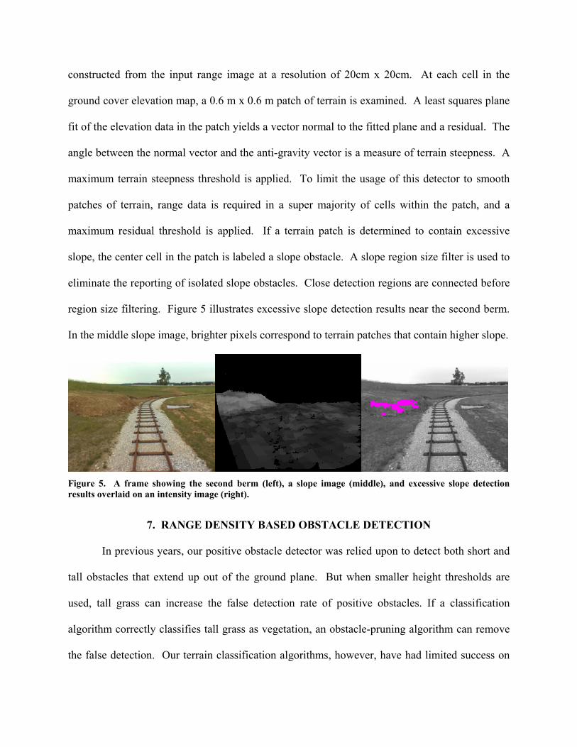
region size filtering. Figure 5 illustrates excessive slope detection results near the second berm.

In the middle slope image, brighter pixels correspond to terrain patches that contain higher slope.

Figure 5. A frame showing the second berm (left), a slope image (middle), and excessive slope detection results overlaid on an intensity image (right).

7. RANGE DENSITY BASED OBSTACLE DETECTION

In previous years, our positive obstacle detector was relied upon to detect both short and

tall obstacles that extend up out of the ground plane. But when smaller height thresholds are

used, tall grass can increase the false detection rate of positive obstacles. If a classification

algorithm correctly classifies tall grass as vegetation, an obstacle-pruning algorithm can remove

the false detection. Our terrain classification algorithms, however, have had limited success on

dry vegetation when the color is very similar to soil. To address this, a range density based

obstacle detector was developed to detect short positive obstacles, such as, stumps and fallen

trees. This enables the positive obstacle detector to be tuned to detect larger objects, such as tall

bushes, people, and other vehicles. For this evaluation, the range density based obstacle detector

has been useful in detecting short dense objects such as the cement blocks.

Range density based obstacle detection is performed in the algorithm that generates a

local terrain map. The density of a cell is the number of range measurements in that cell per unit

volume. Each cell is 20cm long and 20cm wide. The height of a cell is calculated by

differencing the ground cover elevation and the load bearing surface elevation. To determine a

density threshold, we estimate the maximum number of range measurements that could occur in

a cell of a given height. Here, we assume there is a vertical wall across the front edge of a cell.

Since range resolution is a function of range, a portion of the range measurements on a wall at a

given range will lie beyond and before the wall. Assuming this distribution to be normal, we

discount the maximum number of range measurements that could occur in a cell based on the

range of the cell from the sensor. For this analysis, a threshold of 50% was used, i.e., for a cell

to be considered a range density obstacle cell, the total number of range measurements in the cell

must exceed 50% of the theoretical maximum number of range measurements possible for that

cell.

We also require a range density obstacle cell to be a certain height. A single cement

block is approximately 20cm tall. Here, we set the minimum height threshold to 17cm. But

because range resolution degrades with range, it makes no sense to search for 17cm tall objects

at far range. The height threshold was made a linear function of range beyond 5m, where, at a

15m range, the height threshold is 40cm. A region size filter was also implemented to remove

isolated range density obstacle cells. Close range density obstacle cells are connected prior to

region size filtering. In addition, we perform a least squares plane fit on the range data within

each candidate region and threshold the angle between the anti-gravity vector and the normal

vector. This angle should be within a neighborhood centered at 90º for vertical structure. Figure

6 illustrates range density obstacle detection on a frame containing a view of all the stacks of

cement blocks. In the middle range density image, the brighter pixels correspond to cells that

contain higher range density.

Figure 6. A frame showing the four stacks of cement blocks (left), a range density image (middle), and range density obstacle detection results overlaid on an intensity image (right).

8. NEGATIVE OBSTACLE DETECTION

Two complementary negative obstacle detection algorithms were implemented. In the

first, negative obstacle detection is performed on a stereo range image on a column-by-column

basis [2]. As we step up a column in a range image, we search for a gap in the range data

followed by an upward slanting edge. If the gap in the range data exceeds a width threshold and

the height of the edge exceeds a height threshold, the pixel prior to the gap is labeled a candidate

negative obstacle and all of the pixels from the beginning of the gap to the end of the edge are

labeled as supporting negative obstacle pixels. For this data set, a gap threshold of 1m was used.

The edge height threshold used was 50% of the expected visible height given the sensor height,

the distance to the beginning of the gap, and the width of the gap. Once each column is

processed, a connectivity algorithm connects close negative obstacle pixels (supporting or

otherwise). A 3D region size filter then eliminates negative obstacle regions that are too short.

All negative obstacle regions that are less than 1.5m long are eliminated. Only the leading edge

negative obstacle pixels are passed to the local terrain map.

The second negative obstacle detection algorithm was implemented in the software

module that generates local terrain maps. At each cell, we examine neighbor cells in the 8

cardinal directions. If a gap exists that exceeds a gap threshold, and if the cell at the end of the

gap has a minimum elevation lower than the current cell, then the current cell is labeled a

candidate negative obstacle. Close candidate negative obstacles cells are connected and a region

size filter is applied. While the column detector is unidirectional, this detector is omni-

directional. Only the omni-directional negative obstacle regions that intersect the negative

obstacle regions from the column detector are placed within the local terrain map.

Figure 7. A frame showing a portion of the trench oriented parallel to the tracks (left), obstacle detection results overlaid on an intensity image (middle), and a north-oriented local terrain map (right). Multiple obstacle detectors locate different characteristics of the trench.

Figure 7 shows combined obstacle detection on the single trench on the test course. Note

that multiple obstacle detectors locate different portions of the trench. The column based

negative obstacle detector locates the leading edge of the trench (yellow). The magenta overlay

shows where only the omni-directional negative obstacle detector located the trench. Note that

the negative obstacle detection range is increased by several meters by the omni-directional

detector. The vertical wall on the trailing edge of the trench is detected by the positive obstacle

detector (green) and the range density obstacle detector (orange).

9. POSITIVE OBSTACLE DETECTION

Positive obstacle detection is performed on a stereo range image on a column-by-column

basis [2]. As we step up a column in a range image, we search for upward slanted edges. If the

height of an upward slanted edge exceeds a height threshold and the slope of the edge exceeds a

slope threshold, all of the pixels along the edge are labeled positive obstacle pixels. For this data

set, a height and slope threshold of 0.45m and 55º, respectively, was used. Once each column is

processed, a connectivity algorithm connects close positive obstacle pixels. A 3D region size

filter then eliminates small positive obstacle regions. To avoid elimination, a positive obstacle

region has to have either a medium height and large width or a tall height and medium width.

After region size filtering, a leading-edge filter is run that trims positive obstacle pixels that are

likely a part of the ground. Of the remaining positive obstacle pixels, a significant number have

to fall within a cell within the local terrain map for that cell to be labeled a positive obstacle.

While the range density obstacle detector is tuned to detect short objects that a vehicle

can get hung up on, such as rocks, stumps, and fallen trees, the positive obstacle detector is tuned

to detect larger objects, such as trees and tall bushes. Figures 4 and 8 show examples of positive

obstacle detection on the surveyed obstacle course. In Figure 4, a tree trunk wider than 0.3m is

detected as a positive obstacle. In Figure 8, the two bushes at the end of the obstacle course are

detected as positive obstacles.

10. LOW-OVERHANG OBSTACLE DETECTION

The low-overhang obstacle detector was implemented during the PerceptOR program to

detect low-lying branches that could cause damage to the perception sensors [9]. The low

overhang obstacle detector does not detect branches per se. It detects gaps between the top of

ground cover and the bottom of canopy cover and flags the cells containing canopy cover close

enough to the load-bearing surface to cause interference with perception sensors. This detection

is thus performed in the local terrain map, where there are representations of load-bearing

surface, ground cover, and canopy cover elevation. Figure 8 illustrates low-overhang obstacle

detection on the two bushes. Note from the range image that there is a clear gap between the

branches connecting the two bushes and the ground. Several low overhang pixels must exist in a

cell before that cell is labeled a low overhang obstacle cell. This minimizes detecting thin

branches as low overhangs.

Figure 8. A frame showing two closely spaced tall bushes near the end of the test course (left), a 320x240 stereo range image (middle), and obstacle detection results overlaid on an intensity image (right). Blue corresponds to low overhang obstacles and green corresponds to positive obstacles.

11. RESULTS

Table 1 lists the discrete obstacles on the surveyed obstacle course, their dominant

characteristics, the obstacle detectors that located them, and the maximum range (from the

sensors) at which they were detected. Stereo ranging was performed at an image resolution of

320x240 using an 11x11 sum of absolute differences (SAD) correlator. The seven obstacle

detectors were conservatively tuned such that none of them caused false detections anywhere on

the course. Under these conditions, 20 of the 21 obstacles were detected. The single undetected

obstacle was the 4”x4” post. GDRS provided JPL with three ground truth positions. Using a

20cm resolution local terrain map, the obstacle detection algorithms located the single cement

block, a corner of the first man-made water body, and a tree trunk within 5cm, 16cm, and 20cm

of the ground truth positions, at ranges of 2.8m, 5.7m, and 12.9m, respectively.

Table 1. The obstacles located by each obstacle detector for the 1m/s run using wide baseline stereo ranging at an image resolution of 320x240.

Obstacle Type

Dominant Characteristics

Obstacle Detectors

Max Detection Range (m)

Man-made water bodies

Color, low texture, reflections, little range data

Multi-cue water, negative

11.6

Berms High slopes, high range density

Excessive slope, Range density

14.1

Stacks of cement blocks

Short height, high range density

Range density, positive

14.2

PVC poles Tall, thin, vertical, anti-parallel edges

Tree trunk 25.2

Trees Tall, vertical, anti-parallel edges

Tree trunk, positive

16.5

4”x4” post Tall, vertical, anti-parallel edges

Tree trunk, positive

not detected

Trench Gap followed by vertical wall

Negative, positive, range density

15.2

Bushes Tall, wide, connected branches

Positive, low overhang

19.8

The multi-cue water detector located both water bodies. The excessive slope detector

located two of the three berms. The third berm, which was beyond the range of the excessive

slope detector, was located by the range density based detector. The tree trunk detector located

all of the PVC pipes and two of the three tree trunks. The other tree trunk was located by the

positive obstacle detector. There was range density obstacle detection on all three berms, all the

stacks of cement blocks, the vertical wall on the far side of the trench, and the tree trunks. The

positive obstacle detector located several PVC pipes, a stack of cement blocks three high, several

tree trunks, the vertical edge on the far side of the trench, and the two bushes. The negative

obstacle detector located the trench and detected the first water body in a couple of frames. And

the low-overhang detector located the connected branches between the two bushes.

12. CONCLUSIONS

In uncluttered environments where the non-obstacle terrain is equally traversable,

discrete obstacle detection is sufficient. Here, we take a multiple algorithm approach to

detecting a variety of discrete objects with different dominant characteristics. The obstacle

detection algorithms used on the surveyed obstacle course included a positive obstacle detector, a

negative obstacle detector, tree trunk detector, an excessive slope detector, a range density based

detector, a water detector, and a low-overhang detector. Wide baseline stereo imagery was

processed at a resolution of 320x240 for the 1m/s run. All of the obstacles on the course (except

for the single standing 4”x4” post) were detected. There were no false obstacle detections. In

addition, there was complementary detection of several objects by multiple obstacle detectors.

ACKNOWLEDGEMENTS

The research described in this paper was carried out by the Jet Propulsion Laboratory,

California Institute of Technology, and was sponsored by the DARPA PerceptOR program and

the ARL CTA program through agreements with the National Aeronautics and Space

Administration. Reference herein to any specific commercial product, process, or service by

trademark, manufacturer, or otherwise, does not constitute or imply its endorsement by the

United States Government or the Jet Propulsion Laboratory, California Institute of Technology.

REFERENCES

[1] P. Batavia and S. Singh, “Obstacle Detection in Smooth High Curvature Terrain”, Proceedings of the IEEE Conference on Robotics and Automation, Washington D.C., May 2002.

[2] P. Bellutta, R. Manduchi, L. Matthies, K. Owens, and A. Rankin, "Terrain Perception for Demo III", Proceedings of the 2000 Intelligent Vehicles Conference, Dearborn, MI, pp 326-331, October 2000.

[3] T. Chang, T. Hong, S. Legowick, and M. Abrams, “Concealment and Obstacle Detection

for Autonomous Driving”, Proceedings of the IASTED Conference on Robotics and Applications, Santa Barbara, CA, October 1999.

[4] M. Hebert and J. Ponce, “A New Method for Segmenting 3-D Scenes into Primitives”, 6th

International Conference on Pattern Recognition, pp 836-838, October 1982. [5] T. Hong, S. Legowik, and M. Nashman, “Obstacle Detection and Mapping System,

National Institute of Standards and Technology (NIST) Technical Report NISTIR 6213, pp 1-22, 1998.

[6] A. Huertas, L. Matthies, and A. Rankin, “Stereo-Vision Based Tree Traversability

Analysis for Autonomous Off-Road Navigation”, Proceedings of the IEEE Workshop on Applications of Computer Vision, Breckenridge, CO, January 2005.

[7] A. Lacaze, K. Murphy, and M. DelGiorno, “Autonomous Mobility for the Demo III

Experimental Unmanned Vehicles”, Proceedings of the AUVSI Conference, Orlando, July 2002.

[8] R. Manduchi, A. Castano, A. Talukder, and L. Matthies, “Obstacle Detection and Terrain

Classification for Autonomous Off-Road Navigation”, Autonomous Robots, 18, pp 81-102, 2005.

[9] A. Rankin, C. Bergh, S. Goldberg, P. Bellutta, A. Huertas, and L. Matthies, "Passive

Perception System for Day/Night Autonomous Off-Road Navigation", Proceedings of the SPIE Defense and Security Symposium: Unmanned Ground Vehicle Technology VI Conference, Orlando, pp 343-358, March 2005.

[10] A. Rankin, L. Matthies, and A. Huertas, “Daytime Water Detection by Fusing Multiple

Cues for Autonomous Off-Road Navigation”, Proceedings of the 24th Army Science Conference, Orlando, November 2004.

[11] J. Santos-Victor and G. Sandini, “Uncalibrated Obstacle Detection Using Normal Flow”,

Machine Vision Applications, Vol 9, pp 130-137, 1996. [12] A. Talukder, R. Manduchi, A. Rankin, and L. Matthies, "Fast and Reliable Obstacle

Detection and Segmentation for Cross-country Navigation", Proceedings of the 2002 Intelligent Vehicles Conference, France, June 2002.

[13] Z. Zhang, R. Weiss, A.R. Hanson, "Obstacle Detection Based on Qualitative and

Quantitative 3D Reconstruction", IEEE Transactions on Pattern Analysis and Machine Intelligence, 19(1), pp 15-26, 1997 .