evaluation of peakpicking algorithms for protein mass...
TRANSCRIPT

Evaluation of peakpicking algorithms for protein mass spectrometry Book or Report Section
Accepted Version
Bauer, C., Cramer, R. and Schuchhardt, J. (2011) Evaluation of peakpicking algorithms for protein mass spectrometry. In: Hamacher, M., Eisenacher, M. and Stephan, C. (eds.) Data mining in proteomics: from standards to applications. Methods in molecular biology, 696. Humana Press, USA, pp. 341352. ISBN 9781607619864 doi: https://doi.org/10.1007/9781607619871_22 Available at http://centaur.reading.ac.uk/18352/
It is advisable to refer to the publisher’s version if you intend to cite from the work.
To link to this article DOI: http://dx.doi.org/10.1007/9781607619871_22
Publisher: Humana Press
Publisher statement: The original publication is available at www.springerlink.com
All outputs in CentAUR are protected by Intellectual Property Rights law, including copyright law. Copyright and IPR is retained by the creators or other copyright holders. Terms and conditions for use of this material are defined in the End User Agreement .
www.reading.ac.uk/centaur

CentAUR
Central Archive at the University of Reading
Reading’s research outputs online
Evaluation of peak picking algorithms for proteinmass spectrometry
Chris Bauer1,*, Rainer Cramer2, und Johannes Schuchhardt3
1,3MicroDiscovery GmbH, Berlin, Germany2The BioCentre and Department of Chemistry, The University of Reading, Whiteknights,
Reading, RG6 6AS, UK.
December 9, 2010
Abstract
Peak picking is an early key step in MS data analysis. We compare three
commonly used approaches to peak picking and discuss their merits by means of
statistical analysis. Methods investigated encompass signal to noise ratio (SNR),
continuous wavelet transform (CWT) and a correlation-based approach using a
gaussian template.
Functionality of the three methods is illustrated and discussed in a practical
context using a mass spectral data set created with MALDI-TOF technology.
Sensitivity and specificity are investigated using a manually defined reference
set of peaks. As an additional criterion the robustness of the three methods is
assessed by a perturbation analysis and illustrated using ROC curves.
Keywords: Peak picking, SNR, CWT, Gaussian template, Preprocessing, MALDI-
TOF, ROC∗To whom correspondence should be addressed. Email: [email protected]
1
1 Introduction
Peak picking is an early key step in MS based proteomics and crucial for data anal-
ysis. It goes hand in hand with smoothing, baseline correction and peak alignment
within a general workflow of preprocessing steps that allows for subsequent statistical
data analysis and biological interpretation. Preprocessing of MS data aims at trans-
forming a big amount of raw spectral data (usually > 30K data points) into a much
smaller, statistically manageable set of peaks. Subsequent data analysis will typically
aim at biomarker discovery or sample classification. Comprising tens of thousands of
data points in each spectrum, mass spectrometry data is inherently noisy. The main
sources of noise are chemical in nature such as interference from matrix material and
sample contamination or electrical noise which is dependent on the analytical set-up
employed[1]. As a result, various algorithms differing in principle, implementation
and performance have been proposed to address these problems.
A typical preprocessing workflow comprises the following three steps: (See figure
1 for a schematic illustration and exemplary visualization of each step)
• Data Smoothing: Smoothing mainly aims at removing high frequency noise.
Beyond traditional signal processing techniques like Savitzky Golay filter [2],
Mean/Median filter or Gaussian filters also wavelet based techniques are em-
ployed for data smoothing [3],[1].
• Baseline Correction: Baseline correction intends to remove low frequency
noise and thus eliminates the correlation of nearby features. Typically meth-
ods like Top Hat filter[4], Loess derivative filters[5] or linear splines are applied
to estimate the baseline.
• Peak Picking: The number of proposed methods for peak detection is immense.
Most common algorithms make use of signal to noise ratio (SNR), continuous
2
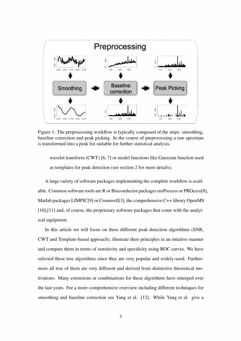
Figure 1: The preprocessing workflow is typically composed of the steps: smoothing,baseline correction and peak picking. In the course of preprocessing a raw spectrumis transformed into a peak list suitable for further statistical analysis.
wavelet transform (CWT) [6, 7] or model functions like Gaussian function used
as templates for peak detection (see section 2 for more details).
A large variety of software packages implementing the complete workflow is avail-
able. Common software tools are R or Bioconductor packages msProcess or PROcess[8],
Matlab packages LIMPIC[9] or Cromwell[3], the comprehensive C++ library OpenMS
[10],[11] and, of course, the proprietary software packages that come with the analyt-
ical equipment.
In this article we will focus on three different peak detection algorithms (SNR,
CWT and Template-based approach), illustrate their principles in an intuitive manner
and compare them in terms of sensitivity and specificity using ROC curves. We have
selected these tree algorithms since they are very popular and widely-used. Further-
more all tree of them are very different and derived from distinctive theoretical mo-
tivations. Many extensions or combinations for these algorithms have emerged over
the last years. For a more comprehensive overview including different techniques for
smoothing and baseline correction see Yang et al. [12]. While Yang et al. give a
3

comprehensive overview on publicly available software briefly describing the applied
methods, our interest in this article is rather the demonstration of the working principle
of the algorithms employed in these public software packages. Following up the eval-
uation of available peak detection algorithms by Yang et al. Liu et al. [13] compared
different feature selection and classification algorithms in a similar way.
1.1 Data set
To evaluate the different algorithms we used data obtained by MALDI-TOF MS anal-
ysis of 259 blood plasma samples from 56 different mice taken at 5 different time
points. Plasma MS profiles were obtained using an Ultraflex MALDI-TOF/TOF mass
spectrometer (Bruker Daltonics, Bremen, Germany). Spectra were acquired automati-
cally for the m/z range of 700-10000. The amount of plasma obtained for each sample
varied between 0 and 12 µl. Since 5 µl were needed for each sample preparation, it
was possible to perform up to two sample preparations. In a few cases only one or
no sample preparation could be performed. From each sample preparation 4 replicate
MALDI spectra were acquired, resulting in a total of up to 8 technical replicates per
sample.
The total number of mass spectra acquired was more than 2100. Prior to any data
processing described in this article technical replications are averaged reducing the
number of spectra to 258. For averaging multiple spectra we applied a peak alignment
strategy[14].
4
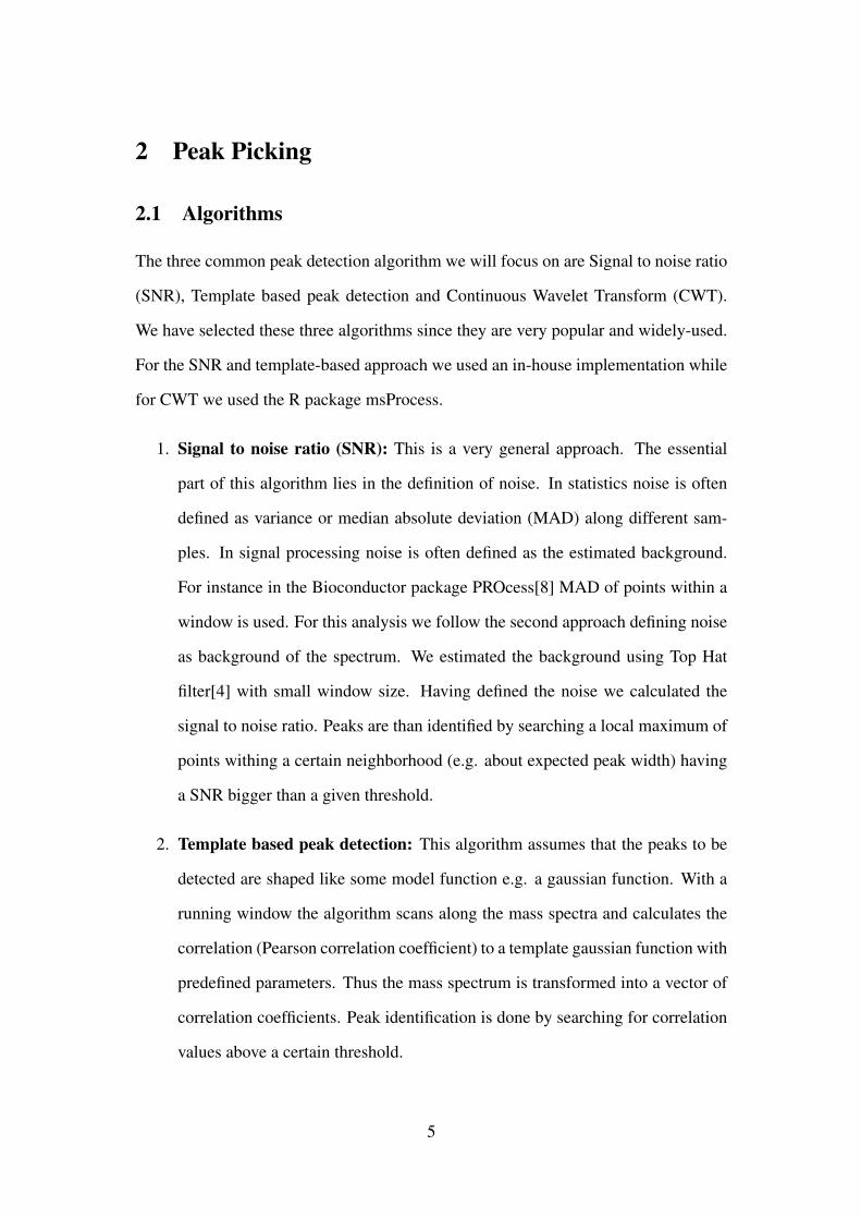
2 Peak Picking
2.1 Algorithms
The three common peak detection algorithm we will focus on are Signal to noise ratio
(SNR), Template based peak detection and Continuous Wavelet Transform (CWT).
We have selected these three algorithms since they are very popular and widely-used.
For the SNR and template-based approach we used an in-house implementation while
for CWT we used the R package msProcess.
1. Signal to noise ratio (SNR): This is a very general approach. The essential
part of this algorithm lies in the definition of noise. In statistics noise is often
defined as variance or median absolute deviation (MAD) along different sam-
ples. In signal processing noise is often defined as the estimated background.
For instance in the Bioconductor package PROcess[8] MAD of points within a
window is used. For this analysis we follow the second approach defining noise
as background of the spectrum. We estimated the background using Top Hat
filter[4] with small window size. Having defined the noise we calculated the
signal to noise ratio. Peaks are than identified by searching a local maximum of
points withing a certain neighborhood (e.g. about expected peak width) having
a SNR bigger than a given threshold.
2. Template based peak detection: This algorithm assumes that the peaks to be
detected are shaped like some model function e.g. a gaussian function. With a
running window the algorithm scans along the mass spectra and calculates the
correlation (Pearson correlation coefficient) to a template gaussian function with
predefined parameters. Thus the mass spectrum is transformed into a vector of
correlation coefficients. Peak identification is done by searching for correlation
values above a certain threshold.
5

3. Continuous Wavelet Transform (CWT): CWT[6, 7] is a more sophisticated
approach that is used to split the signal into different frequency ranges. Regard-
ing the m/z scale as generalized time scale, CWT constructs a time-frequency
representation of the spectrum by mapping it from the time domain to the time-
scale domain. The essential part of CWT is the mother wavelet whose translated
and scaled versions are used to generate daughter wavelets. The mother function
we used for this evaluation is the second derivative of a gaussian function (Mex-
ican Hat Wavelet). Peak picking typically includes the inspection of multiple
scales. For peak detection (using R package msProcess) the peak candidate has
to be clearly distinguishable from the background (parameter: snr.min) and vis-
ible across at least 7 scale domains (parameter: length.min) excluding the first
three high frequency wavelet scales (parameter: scale.min). Excluding high fre-
quency wavelets acts as filter for high frequency noise.
2.2 Reference Peaks
In order to evaluate the peak picking algorithms we defined a set of reference peaks.
A peak picking algorithm can then be evaluated in terms of sensitivity (how many of
the reference peaks are found) and specificity (how many of the found peaks are part
of the reference set). An optimal algorithm has high sensitivity and high specificity.
The reference set was created in a semi-automatic process. To this end we initially
picked peaks manually and subsequently optimized peak positions automatically. This
procedure ensures a high quality reference set containing very prominent peaks as well
as peaks situated in the rising or falling edge of another peak or peaks with poor signal
intensities. All in all the reference set contained a total of 381 peaks.
6
0.1
0.2
0.3
0.4
0.5
0.6
Inte
nsity
SpectrumNoiseref peaks
A
12
34
5
SN
R
SNRThresholdref Peaks
B
−0.
50.
00.
51.
0
Cor
rela
tion Correlation
Thresholdref Peaks
C
1500 1600 1700 1800
−0.
20.
00.
20.
40.
6
m/z
Inte
nsity
Waveletsref Peaks
D
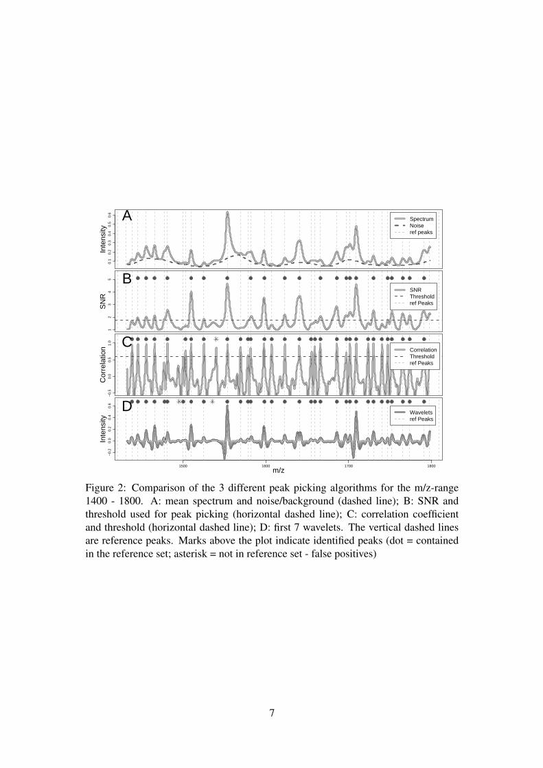
Figure 2: Comparison of the 3 different peak picking algorithms for the m/z-range1400 - 1800. A: mean spectrum and noise/background (dashed line); B: SNR andthreshold used for peak picking (horizontal dashed line); C: correlation coefficientand threshold (horizontal dashed line); D: first 7 wavelets. The vertical dashed linesare reference peaks. Marks above the plot indicate identified peaks (dot = containedin the reference set; asterisk = not in reference set - false positives)
7

2.3 Comparing peak picking algorithms
Figure 2 gives a graphical impression of how the different algorithms are working.
The first box shows the mean intensity spectrum of the complete data set in a mass
window of 1400-1800 Da. The noise level was defined as baseline calculated using
Top Hat filter (see dashed line). The 33 peaks from the reference set within this mass
window (see section 2.2) are indicated as vertical dashed lines.
The second part of figure 2 shows the signal to noise ratio along the mass window
of the mean spectrum. The SNR threshold used for peak identification was 1.75 indi-
cated as horizontal dashed line. Using SNR we identified 22 peaks in this mass range
whereas we found 69% of our reference peaks (with the SNR threshold of 1.75). With
this threshold we did not find any peak that was not part of the reference set.
The third box in figure 2 visualizes the performance of template-based peak de-
tection. The correlation coefficients along the spectrum are shown. The correlation
threshold of 0.6 is indicated as horizontal dashed line. All in all we found 31 of the 33
reference peaks (94%) indicated as dots above the peaks. We also found one peak that
is not within the reference set (false positive) shown as asterisk above the peak.
The last part of figure 2 demonstrates the peak picking using wavelet transform.
The first 7 daughter wavelets are shown. Compared to the other two methods the
peak picking is complicated by the fact that information from different time-scale
domains has to be combined (see chapter 2.1 for more details). The reference peaks
again appear as vertical dashed lines and the picked peaks are marked above the peaks.
Using CWT we identified 97% of the peaks but also got two false positive hits (marked
with asterisks above the peaks).
8

0.0 0.2 0.4 0.6 0.8 1.0
0.0
0.2
0.4
0.6
0.8
1.0
ROC Curve for Peak Picking
1−Specificity
Sen
sitiv
ity
SNRCorrelationCWT
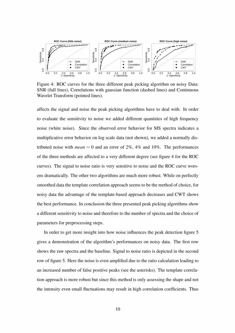
Figure 3: ROC curves presenting the performance of the three different peak pickingalgorithms: SNR (full line), Correlations with gaussian function (dashed line) andContinuous Wavelet Transform (pointed line). The ROC curves are calculated byscanning the threshold values of the different algorithms.
2.4 Evaluating peak picking algorithms
As already mentioned in section 2.2 the reference peak set can be used to calculate val-
ues for sensitivity and specificity. That in turn can be used to generate ROC curves (see
figure 3). ROC curves are calculated by scanning the threshold values of the different
algorithms e.g. changing the correlation threshold in the template based approach (for
an illustration of the threshold operation see figure 2).
2.4.1 Stability
The combination of smoothing and baseline correction defines a bandpassfilter re-
moving high and low frequency noise. Parameter tuning of those preprocessing steps
9
0.0 0.2 0.4 0.6 0.8 1.0
0.0
0.4
0.8
ROC Curve (little noise)
1−Specificity
Sen
sitiv
ity
SNRCorrelationCWT
0.0 0.2 0.4 0.6 0.8 1.0
0.0
0.4
0.8
ROC Curve (medium noise)
1−Specificity
Sen
sitiv
ity
SNRCorrelationCWT
0.0 0.2 0.4 0.6 0.8 1.0
0.0
0.4
0.8
ROC Curve (high noise)
1−Specificity
Sen
sitiv
ity
SNRCorrelationCWT
Figure 4: ROC curves for the three different peak picking algorithm on noisy Data:SNR (full lines), Correlations with gaussian function (dashed lines) and ContinuousWavelet Transform (pointed lines).
affects the signal and noise the peak picking algorithms have to deal with. In order
to evaluate the sensitivity to noise we added different quantities of high frequency
noise (white noise). Since the observed error behavior for MS spectra indicates a
multiplicative error behavior on log scale data (not shown), we added a normally dis-
tributed noise with mean = 0 and an error of 2%, 4% and 10%. The performances
of the three methods are affected to a very different degree (see figure 4 for the ROC
curves). The signal to noise ratio is very sensitive to noise and the ROC curve wors-
ens dramatically. The other two algorithms are much more robust. While on perfectly
smoothed data the template correlation approach seems to be the method of choice, for
noisy data the advantage of the template-based approach decreases and CWT shows
the best performance. In conclusion the three presented peak picking algorithms show
a different sensitivity to noise and therefore to the number of spectra and the choice of
parameters for preprocessing steps.
In order to get more insight into how noise influences the peak detection figure 5
gives a demonstration of the algorithm’s performances on noisy data. The first row
shows the raw spectra and the baseline. Signal to noise ratio is depicted in the second
row of figure 5. Here the noise is even amplified due to the ratio calculation leading to
an increased number of false positive peaks (see the asterisks). The template correla-
tion approach is more robust but since this method is only assessing the shape and not
the intensity even small fluctuations may result in high correlation coefficients. Thus
10

0.1
0.2
0.3
0.4
0.5
0.6
0.7
Inte
nsity
SpectrumNoiseref peaks
A1
23
45
SN
R
SNRThresholdref Peaks
B
−0.
50.
00.
51.
0
Cor
rela
tion Correlation
Thresholdref Peaks
C
1500 1600 1700 1800
−0.
20.
00.
20.
40.
6
m/z
Inte
nsity
Waveletsref Peaks
D
Figure 5: Comparison of the 3 different peak picking algorithms on noisy data forthe m/z range of 1400 - 1800. High frequency noise was added to the spectrum asdescribed in the text. A: mean spectrum and background (dashed line); B: SNR andthreshold used for peak picking (horizontal dashed line); C: correlation coefficientand threshold (horizontal dashed line); D: first 7 wavelets. The vertical dashed linesare reference peaks. Marks above the plot indicate peaks identified with the differentalgorithms (dot = contained in the reference set; asterisk = not in the reference set).
peaks are not clearly distinguishable from background noise any more. For noisy data
CWT outperforms the other methods since CWT intrinsically acts like a smoothing
filter on the data. Even if the first wavelets are noisy, the lower frequency scales are
very smooth (see lower row of figure 5). Hence high frequency noise does not affect
the algorithm’s performance strongly as high frequency wavelets that include most of
the noise are filtered out.
11
3 Discussion
The three different peak picking algorithms investigated here are distinct in terms of
complexity, performance and stability. But all three methods have a common param-
eter: the estimated peak width. There are different ways to estimate the optimal peak
width. For instance OpenMS [10],[11] as a freely available MS processing library
offers the possibility to measure the peak width manually using graphical interface or
the peak width can be estimated by the CWT algorithm itself.
For an overview of the advantages and disadvantages of the algorithms see table 1.
Signal to noise ratio as a universally used signal processing technique is computation-
ally fast, easy to implement and shows good performance on smoothed data. However,
it is not very specific for this task as it ignores the shape of the peak. Since the noise
is an integral part of the algorithm it is very sensitive to noise and therefore strongly
depends on the quality of the data and on the performance of previously performed
smoothing and baseline correction steps.
The template-based approach is much more specific for the peak picking task as-
suming peaks to be shaped like a gaussian function. This assumption, however, might
often not be exactly applicable because peaks may show a considerable asymmetry.
Depending on the experimental parameters, particularly laser energy, significant devi-
ation from a Gaussian peak shape can be globally obtained. Although this method has
only a few parameters, it appears rather robust for lower levels of noise. However for
high levels of noise the performance decreases.
CWT is like SNR a very universal signal processing technique used for many dif-
ferent tasks. Contrary to SNR the algorithm is complex and is computationally expen-
sive. The large number of parameters allows for tuning CWT to be very specific for
this task taking into account the shape of the peak. As smoothing is an intrinsic part of
the algorithm CWT is very robust even for substantial amounts of noise. On the other
12

Method PRO CONTRA
SNR
• simple - easy to implement
• fast performance
• only few parameters
• depends on the definition ofnoise
• unstable - very sensitive tonoise
• ignoring peak shape
TemplateCorrelation
• simple - easy to implement
• only few parameters
• stable for small noise
• detection favors gaussianshaped peaks
• sensitive to high noise
CWT
• stable even for massive noise
• internal data smoothing
• flexible - tuneable
• complicated algorithm
• slow performance
• difficult to tune - high numberof parameters
Table 1: Summary of advantages and disadvantages of the three presented peak pick-ing algorithms.
hand tuning of the algorithm is difficult due to the large set of parameters.
For perfectly smoothed data all three methods show good performances but CWT
seems to be little worse than the other two. For data including a substantial amount
of noise CWT clearly outperforms the other methods in terms of sensitivity and speci-
ficity.
Both, the template based approach and CWT show good performances includ-
ing a robustness for noise. Figure 6 shows two example peaks for the different peak
detection using these two algorithms. In the upper row the peak at m/z 1846 was iden-
tified only with CWT while in the lower row the peak at m/z 4052 was detected only
with the template-based method. The shortcoming of the template-based approach is
clearly visible since the peak at m/z 1846 is not shaped like a gaussian function result-
ing in lower correlation coefficients. Hence this peak could not be detected using a
gaussian function as template. In contrast the peak at m/z 4052 shows a good match-
ing gaussian shape, facilitating peak detection by correlation. CWT does not find this
peak since there are not enough wavelets above threshold (in this case there are only
13

1840 1850
0.06
0.10
0.14
Peak at 1846.58
Mass
Inte
nsity
1840 1850−1.
0−
0.5
0.0
0.5
1.0
Correlation
MassC
orre
latio
n
1840 1850
−0.
050.
050.
10
CWT
Mass
Wav
elet
s4040 4050 4060
0.15
0.20
0.25
Peak at 4052.05
Mass
Inte
nsity
4040 4050 4060−1.
0−
0.5
0.0
0.5
1.0
Correlation
Mass
Cor
rela
tion
4040 4050 4060−
0.1
0.0
0.1
0.2
0.3
CWT
Mass
Wav
elet
s
Figure 6: Peaks found with CWT and not with template based approach (upper part)and vice versa (lower part), first column: spectrum, second column: correlation co-efficient and correlation threshold, third column: first 9 wavelets and noise (dashedline).
5 wavelets above the noise level but the algorithm requires at least 7).
The reference set we used for evaluation was manually created assuming the hu-
man eye to be a good peak detector. With this procedure we assure that the reference
set is constructed without giving preference to any algorithm. Looking at the spectra
and the visualization of the three algorithms (figure 2) we see that there is one peak
identified with correlation based approach and CWT (indicated as asterisks) and even
with a higher SNR that was not classified as a peak using the human eye. However,
remarkably the three algorithms differ in exactly this peak underlining that in general
peak picking is a non-trivial task.
14

4 Notes:
Õ For MALDI-TOF data adequate preprocessing is required in order to allow sub-
sequent statistical data analysis such as biomarker discovery or sample classifi-
cation.
Õ Preprocessing workflow typically comprises algorithms for data smoothing such
as Mean filter or Savitzki Goley filter, baseline correction like Top Hat filter or
Loess derived filters and peak picking such as SNR, CWT or template based
approaches.
Õ The main objective is to transform the big amount of raw spectral data into a
much smaller, statistically manageable set of peaks.
Õ The number of algorithms implementing peak picking is large. The various
algorithms differ in performance, implementation and theoretical motivation.
Õ Various common software tools are available designed to address the prepro-
cessing workflow. They are based on different platforms including R and Matlab
packages as well as stand-alone C++ applications.
Õ Approaches based on SNR are rather simple, easy to use and fast but also sensi-
tive for noise. Moreover the shape of the peak is ignored completely.
Õ Template-based approaches are simple, easy to use and robust to limited noise.
But they can only detect peaks shaped like the used template function and they
are vulnerable to strong noise.
Õ CWT shows good performances and is stable even for strong noise but more
complicated, difficult to tune and therefore harder to use and understand.
Õ Every algorithm has pros and cons as it fails in finding certain types of peaks.
15

Template based approach fails to detect peaks differing in shape from used tem-
plate. CWT tends to miss thin peaks surrounded by higher ones.
Õ The definition of the reference peak set is a crucial step for evaluating the dif-
ferent algorithms. Neither the human eye nor some automatic peak detection
algorithm can guarantee to detect all peaks. Still, regarding a sensitivity and
specificity of 0.9, the majority of the peak show good agreement of the used
algorithms and the human eye.
References
[1] D. Kwon, M. Vannucci, J.J. Song, J. Jeong, and R.M. Pfeiffer. A novel wavelet-
based thresholding method for the pre-processing of mass spectrometry data that
accounts for heterogeneous noise. Proteomics, 8:3019–3029, Aug 2008.
[2] Abraham Savitzky and Marcel J.E. Golay. Smoothing and differentiation of data
by simplified least squares procedures. Analytical Chemistry, 36(8):1627–1639,
1964.
[3] K.R. Coombes, S. Tsavachidis, J.S. Morris, K.A. Baggerly, M.C. Hung, and
H.M. Kuerer. Improved peak detection and quantification of mass spectrome-
try data acquired from surface-enhanced laser desorption and ionization by de-
noising spectra with the undecimated discrete wavelet transform. Proteomics,
5:4107–4117, Nov 2005.
[4] Anne C Sauve and Terence P. Speed. Normalization, baseline correction and
alignment of high-throughput mass spectrometry data. 2004.
[5] W.S. Cleveland, E. Grosse, and W.M. Shyu. Local regression models, pages pp.
309–376. Wadsworth, 1992.
16

[6] E. Lange, C. Gropl, K. Reinert, O. Kohlbacher, and A. Hildebrandt. High-
accuracy peak picking of proteomics data using wavelet techniques. Pac Symp
Biocomput, pages 243–254, 2006.
[7] P. Du, W. A. Kibbe, and S. M. Lin. Improved peak detection in mass spectrum
by incorporating continuous wavelet transform-based pattern matching. Bioin-
formatics, 22:2059–2065, Sep 2006.
[8] Robert Gentleman and Vince Carey and Wolfgang Huber and Rafael Irizarry and
Sandrine Dudoit, editor. Bioinformatics and Computational Biology Solutions
Using R and Bioconductor. Springer Verlag, 2005.
[9] D. Mantini, F. Petrucci, D. Pieragostino, P. Del Boccio, M. Di Nicola, C. Di Ilio,
G. Federici, P. Sacchetta, S. Comani, and A. Urbani. LIMPIC: a computational
method for the separation of protein MALDI-TOF-MS signals from noise. BMC
Bioinformatics, 8:101, 2007.
[10] O. Kohlbacher, K. Reinert, C. Gropl, E. Lange, N. Pfeifer, O. Schulz-Trieglaff,
and M. Sturm. TOPP–the OpenMS proteomics pipeline. Bioinformatics,
23:e191–197, Jan 2007.
[11] M. Sturm, A. Bertsch, C. Gropl, A. Hildebrandt, R. Hussong, E. Lange,
N. Pfeifer, O. Schulz-Trieglaff, A. Zerck, K. Reinert, and O. Kohlbacher.
OpenMS - an open-source software framework for mass spectrometry. BMC
Bioinformatics, 9:163, 2008.
[12] C. Yang, Z. He, and W. Yu. Comparison of public peak detection algorithms for
MALDI mass spectrometry data analysis. BMC Bioinformatics, 10:4, 2009.
[13] Q. Liu, A. H. Sung, M. Qiao, Z. Chen, J. Y. Yang, M. Q. Yang, X. Huang, and
Y. Deng. Comparison of feature selection and classification for MALDI-MS
data. BMC Genomics, 10 Suppl 1:S3, 2009.
17

[14] N. Jeffries. Algorithms for alignment of mass spectrometry proteomic data.
Bioinformatics, 21:3066–3073, Jul 2005.
18