evaluation of bic-based algorithms for audio segmentation · evaluation of bic-based algorithms for...

COMPUTER
SPEECH AND
Computer Speech and Language 19 (2005) 147–170LANGUAGE

www.elsevier.com/locate/csl

Evaluation of BIC-based algorithms for audio segmentation

Mauro Cettolo a,*, Michele Vescovi b, Romeo Rizzi b

a ITC-irst, Centro per la Ricerca Scientifica e Tecnologica, Via Sommarive, 18 I-38050 Povo, Trento, Italyb Universit�a degli Studi di Trento, Facolt�a di Scienze MM.FF.NN. I-38050 Povo, Trento, Italy

Received 24 June 2003; received in revised form 24 May 2004; accepted 26 May 2004

Available online 1 July 2004

Abstract

The Bayesian Information Criterion (BIC) is a widely adopted method for audio segmentation, and has

inspired a number of dominant algorithms for this application. At present, however, literature lacks in

analytical and experimental studies on these algorithms. This paper tries to partially cover this gap.Typically, BIC is applied within a sliding variable-size analysis window where single changes in the

nature of the audio are locally searched. Three different implementations of the algorithm are described and

compared: (i) the first keeps updated a pair of sums, that of input vectors and that of square input vectors,

in order to save computations in estimating covariance matrices on partially shared data; (ii) the second

implementation, recently proposed in literature, is based on the encoding of the input signal with cumu-

lative statistics for an efficient estimation of covariance matrices; (iii) the third implementation consists of a

novel approach, and is characterized by the encoding of the input stream with the cumulative pair of sums

of the first approach.Furthermore, a dynamic programming algorithm is presented that, within the BIC model, finds a

globally optimal segmentation of the input audio stream.

All algorithms are analyzed in detail from the viewpoint of the computational cost, experimentally

evaluated on proper tasks, and compared.

� 2004 Elsevier Ltd. All rights reserved.

* Corresponding author. Tel.: +39-0461-314-551; fax: +39-0461-314-591.

E-mail addresses: [email protected] (M. Cettolo), [email protected] (M. Vescovi), [email protected]

(R. Rizzi).

0885-2308/$ - see front matter � 2004 Elsevier Ltd. All rights reserved.

doi:10.1016/j.csl.2004.05.008

mail to: [email protected]

148 M. Cettolo et al. / Computer Speech and Language 19 (2005) 147–170

1. Introduction

In the last years, efforts have been devoted amongst the research community to the problem ofaudio segmentation. The number of application of this procedure is considerable: from the ex-traction of information from audio data (e.g., broadcast news, recording of meetings) to theautomatic indexing of multimedia data, or the improvement of accuracy for recognition systems.Typically, these tasks are performed by complex systems, consisting of a number of modules,some of them computationally expensive. Although in these systems the audio segmentation doesnot represent a computational bottleneck, the response time of the segmentation module canbecome an important issue under specific requirements. For example, ITC-irst delivered to RAI(the national Italian broadcasting company) an off-line system for the automatic transcription ofbroadcast news programs. Part of the requirement was also to supply a real-time version of thetranscription station, able to guarantee adequate performance. Given these constraints, the speedof each component needs to be maximized without affecting its accuracy.

The segmentation problem has been handled in different ways that can be roughly grouped inthree classes:

energy based methods: each silence occurring in the input audio stream is detected either byusing an explicit model for the silence or by thresholding the signal energy. Segment boundariesare then located in correspondence of detected silences.metrics based methods: the segmentation of the input stream is achieved by evaluating its‘‘distance’’ from different segmentation models. Distances can be measured by the Hotelling’sT 2 test (Wegmann et al., 1999), the Kullback Leibler distance (Kemp et al., 2000; Siegler et al.,1997), the generalized likelihood ratio (Gish et al., 1991), the entropy loss (Kemp et al., 2000),and the Bayesian Information Criterion (BIC) (Schwarz, 1978).explicit models based methods: models are built for a given set of pre-determined acousticclasses – e.g., female and male speakers, music, noise, etc. Typically, the input data stream isclassified from the maximum likelihood principle, through a dynamic programming decoding.The time indexes where the classification changes from one class to another are assumed to bethe segment boundaries (Hain et al., 1998). Alternatively, in (Lu et al., 2001) Support VectorMachines are employed to learn class boundaries; (Scheirer and Slaney, 1997) compares theGaussian Maximum A-Posteriori estimator, the Gaussian Mixture Model, the Nearest-Neigh-bor classifier and a spatial partitioning scheme based on K-d trees.The main limitations of the first and the third approach are evident. Regarding the energy

based methods, there is only a partial correlation between changes in the nature of the audio andsilences. On the other hand, these methods are simple to implement and can perform their(limited) task in linear time and with sufficient precision – provided the absence of significantvariations in the background acoustic conditions. With explicit models of acoustic classes,changes occurring within the same class are undetectable; for example, if only one model forfemale voices is employed, no change can be detected within a dialogue between female speakers.Moreover, it is required both to know in advance the classes of interest and the availability ofsuitable data for their training. On the other hand, these methods can reach very high accuracyrates with linear time cost complexity.

This paper concentrates on a specific class of metric-based methods. Metric-based methods donot require any prior knowledge, nor a training stage. They are efficient (linear in time if some

M. Cettolo et al. / Computer Speech and Language 19 (2005) 147–170 149

approximations are introduced – as shown later), simple to implement and are able to give goodresults. This explains why in a lot of laboratories much attention has been devoted to this type ofmethods, and in particular to the BIC (Cettolo, 2000; Cettolo and Vescovi, 2003; Chen andGopalakrishnan, 1998; Delacourt et al., 1999; Harris et al., 1999; Sivakumaran et al., 2001;Tritschler and Gopinath, 1999; Vescovi et al., 2003; Wellekens, 2001). Typically, the BIC ‘‘dis-tance’’ is used locally, within a shift variable-size window, where single changes in the nature ofaudio are searched. In this paper, we deal with metric-based audio segmentation algorithms basedon the BIC.

In the research community it is customary to combine different (almost orthogonal) solutions toexploit advantages and circumvent limitations. This is also the case of audio segmentation.Usually, real systems include a partitioning module that segments, classifies and clusters the audiostream via a combination of different algorithms. Among the most successful systems we findindeed highly integrated partitioning modules, as for example in Gauvain et al. (1998) and in Hainet al. (1998). Even if this trend has allowed the development of very competitive systems, this hasled to the situation where it is difficult to have a clear insight on how to improve the state of theart.

As a matter of fact, literature regarding analytical and experimental studies of segmentationalgorithms remains – somewhat – limited. The only known exception is Sivakumaran et al. (2001),where an efficient approach to the local BIC-based segmentation algorithm is proposed and itscomputational cost briefly analyzed. However, only a very limited comparison with other algo-rithms is given. In that work, the input audio stream is progressively encoded by cumulativestatistics, and the encoding is exploited to avoid redundant operations in the computation of BICvalues.

In this paper, we try to cover part of the studies on segmentation algorithms by proposing: (i)an innovative method for the implementation of the BIC-based local algorithm – this guar-antees (to the best of our knowledge) the lowest computational cost; (ii) a global algorithmcapable of finding the optimal BIC input segmentation – this represents the performance upperbound for the class of the BIC-based segmentation algorithms. The algorithms are describedand compared, both analytically and experimentally, with the method given in Sivakumaranet al. (2001).

The paper is organized as follows. In Section 2, a general definition of the audio segmentationproblem is given.

Section 3 presents the corpora used for experiments, together with the evaluation measures; abrief description of the signal processing front-end is also given.

In Section 4, the BIC-based local algorithm as proposed in Delacourt et al. (1999) is described,building on the general framework provided in Section 2. The computational cost of the localalgorithm presented in Sivakumaran et al. (2001) is analyzed in detail (Section 4.1.2) and com-pared, both in theory and experimentally, with the cost of two other possible approaches: onemore direct but more expensive, which represents a reference (Section 4.1.1); and a novel methodthat combines the good ideas of the other two (Section 4.1.3). On a test set of broadcast newsprograms, the new approach is 35% faster than the one proposed in Sivakumaran et al. (2001)(Section 4.2).

Section 5 presents, within the general framework of Section 2, a Dynamic Programming (DP)algorithm which uses the BIC method to find the globally optimal segmentation of the input


audio. The algorithm with its computational costs are described in detail. It is also compared tothe most efficient implementation of the local algorithm. On the 2000 NIST Speaker RecognitionEvaluation test set, the global algorithm outperforms the local one by 2.4% (relative) F -score inthe detection of changes, but is 38 times slower.

A summary ends the paper.

2. The segmentation problem and the BIC

Segmenting an audio stream consists of detecting the time indexes corresponding to changes inthe nature of the audio, this to isolate segments that are acoustically homogeneous. This can beseen as a particular instance of the more general problem of partitioning data into distinct ho-mogeneous regions (Baxter, 1996). The data partitioning problem arises in all applications thatrequire partitioning data into chunks, e.g., image processing, data mining, text processing, etc.

The problem can be formulated as follows. Let O ¼ o1; o2; . . . ; oN be an ordered sequence ofobservations, called the sample, in which each oi is a vector in Rd . We assume that the sample isgenerated by a Gaussian process with a certain number of transitions. The problem of segmen-tation is that of detecting all the transition points in the data set. In the ambit of acoustic seg-mentation, transitions correspond to changes in the nature of the audio, represented by thesample O.

A particular model of the input data is characterized by a specific number c of changes and aspecific set f16 t1; t2; . . . ; tc < Ng of time indexes corresponding to these changes. In such a way,the input data are modeled by a set of cþ 1 Gaussian distributions, each one generating anobservation subsequence bounded by two consecutive time indexes out of f1; t1; . . . ; tc;Ng.

Among all possible models of the sample, the ‘‘best’’ one has to be selected, and its timeindexes will define the segmentation of the input stream. The best model is the one that betterfits the observations. The application of the maximum likelihood principle would however in-variably lead to choosing the model with the maximum number of changes (cmax ¼ N � 1), asthis model has the highest number of free parameters. In order to take into account the notionof ‘‘dimension’’ of the model, the following extension to the maximum likelihood principle wasfirst proposed by Akaike (1977). The AIC (Akaike’s Information Criterion) suggests to maxi-mize the likelihood for each model Mi separately, obtaining say LMi ¼ LMiðOÞ, and then choosethe model for which ðlog LMi � FMiÞ is largest, where FMi is the number of free parameters of themodel Mi.

Several model selection criteria that can be applied to Akaike’s framework of model selectionhave been proposed in the literature (see Cettolo and Federico, 2000 for a review). In general, eachcriterion proposes the introduction of a penalty function P that takes into account the dimensionof the model.

The BIC is the penalty function proposed in Schwarz (1978), and is defined as

PM ¼ FM2

logN : ð1Þ

As an example, let us consider a sample of three observations O ¼ o1; o2; o3. The possible modelsof O to be compared are:


• a 1-Gaussian process (let it be M1):

o1; o2; o3 �iid Ndðl;RÞ;
• two 2-Gaussians processes (M2 and M3):
o1; o2 �iid NdðlA;RAÞ;

o3 �iid NdðlB;RBÞ
and:
o1 �iid NdðlA;RAÞ;

o2; o3 �iid NdðlB;RBÞ;
• a 3-Gaussians process (M4):
o1 �iid NdðlA;RAÞ;

o2 �iid NdðlB;RBÞ;

o3 �iid NdðlC;RCÞ:
Once ðlogLMiðOÞ � PMiÞ has been computed for each i ¼ 1; 2; 3; 4, the highest value gives thewinner model. If it is, for example, M2, the best segmentation of O under the BIC consists of thefollowing two segments: ðo1o2Þ and ðo3Þ.
2.1. Search

Given the set fMig of possible models of the input sequence, the segmentation problem nowreduces to solve the following maximization:

imax ¼ argmaxi logLMi � PMi : ð2Þ
Instead of explicitly listing the set of all possible models, whose size is Of2Ng, polynomial searchalgorithms can be employed. A widely adopted search algorithm uses a sliding variable-sizeanalysis window, where the maximization given above is used to detect single changes. That is,models compared in Eq. (2) have only one transition or none at all. The algorithm and threeimplementations with different computational costs are described in Section 4. The algorithmmain limitation is that the search is done locally – hence the objective function that determines themost plausible interpretations of the input audio stream is not globally maximized. In principle,this could affect the effectiveness of the method, especially if the audio stream includes manychanges close to each other – as in the case of human–human conversations. In Section 5, a globalalgorithm able to find the solution of Eq. (2) in the BIC framework, is presented.
3. Data sets and evaluation measures

Two corpora were selected for experiments, namely the Italian Broadcast News Corpus (IBNC)and the 2000 NIST Speaker Recognition Evaluation corpus. The two collections are substantially


different in the nature of audio recordings, allowing the evaluation of algorithms under verydifferent working conditions.

3.1. The IBNC corpus

The IBNC corpus (Federico et al., 2000), collected by ITC-irst and available through ELDA,the Evaluations and Language resources Distribution Agency (IBNC, 2000), is a speech corpus ofradio broadcast news in Italian. It consists of 150 recordings, for a total of about 30 h, coveringradio news of several years. Data were provided by RAI. The corpus presents variations of topics,speakers, channel band (i.e., studio versus telephone), speaking mode (i.e., spontaneous versusplanned), etc. It has been manually transcribed, segmented and labeled. Speaker gender and, whenpossible, identity are also annotated.

For testing purposes, six programs (about 75 min of audio) were selected, where 212 changesoccur, between either different speakers or different acoustic classes (music, speech, noise, etc.).

In broadcast news, acoustically homogeneous segments are typically long. This makes IBNCdata suitable for assessing the ability of segmentation algorithms in the detection of changesaround which much homogeneous data is available.

3.2. The 2000 NIST speaker recognition evaluation

The 2000 NIST Speaker Recognition Evaluation (NIST, 2000) included a segmentation task,where systems were required to identify speech segments corresponding to each of two unknownspeakers. The test set consists of 1000 telephone conversations, lasting about 1 min each, includedin the Disc r65_6_1. 777 Speakers, of both genders, pronounced a total of 46K turns/segments.Fig. 1 shows the distribution of segment length. The longest segment is 26.5 s; the mean length is1.3 s, while the median is less than 1 s; it is worth noticing that 81% of segments has length lower

0

2

4

6

8

10

12

0 0.5 1 1.5 2 2.5 3 3.5 4

% s

egm

ents

segment length (seconds)

Fig. 1. Distribution of length of NIST test set segments.


than 2 s. This means that the NIST data are suitable to make evident if segmentation algorithmsare able to detect changes bounding very short segments.

The NIST test set was also employed in this work. For evaluation, we relied on a referencesegmentation obtained by merging the two reference segmentations provided by NIST for eachspeaker. It was observed that often the end of a sentence of a speaker does not exactly correspondto the beginning of the successive sentence of the other speaker: this is due either to small im-precision of the manual annotation, or to a short overlap of the sentences, or to a brief silenceoccurring between the two sentences. In such cases, short segments created when merging wereremoved by an automatic procedure.

3.3. Evaluation measures

Performance of automatic change detection is calculated with respect to a set of target changes.Tolerances in the detection can be introduced, e.g., �0.5 s: in such a way the target is an intervalrather than a single time index.

For comparing target and hypothesized changes, we adopt the precision P and the recall Rmeasures:

P ¼ ccþ i

� 100;

R ¼ ccþ d

� 100;

where c is the number of target intervals which contain at least one hypothesized change, i is thenumber of hypothesized changes that do not fall inside any target interval (insertions), and d is thenumber of target intervals which contain no hypothesized change (deletions). In other words,precision is related to the number of false alarms, i.e., the number of wrongly split segments, whilerecall measures the deletion rate of correct changes, i.e., the number of wrongly merged segments.

The evaluation of the segmentation quality is made in terms of F-score, a combined measure ofP and R of change detection. F -score is a measure proposed by van Rijsbergen (Frakes and Baeza-Yates, 1992) and is defined as

F ¼ ð1þ b2ÞPRb2P þ R

;

where b is a measure of the relative importance, to a user, of precision and recall. For example, blevels of 0.5, indicating that a user was twice as interested in precision as recall, and 2, indicatingthat a user was twice as interested in recall as precision, might be used. The most popular valuecorresponds to b ¼ 1, for which F reduces to

F ¼ 2PRP þ R

:

In this paper b was set to 1.Concerning the NIST data set, after the official evaluation, NIST made available both the

reference segmentations of the test files and a scoring script. The scoring script computes thesegmentation error rate, i.e., the percentage of speech from one speaker wrongly assigned to


the other speaker. The measure is suitable for the NIST task which, by definition, is a classifi-cation task. On the contrary, the algorithm presented here detects speaker/spectral changes, andno attempt is done to classify segments in terms of speakers. The NIST scoring script does nottherefore fit with our evaluation requirements.

In fact, precision and recall (or the corresponding false alarm and miss detection rates) aremetrics that better assess the performance of the change detection algorithm. For this reason, thetwo metrics and their F -score are also used in the evaluation of the algorithms with the NIST dataset.

3.4. Audio processing

Multivariate observations derive from a short time spectral analysis, performed over 20 msHamming windows at a rate of 10 ms. For every window, 12 Mel scaled Cepstral coefficients andthe log-energy are evaluated.

4. Local search: an approximated algorithm

First of all, let us recall some basic results. Given a sample O ¼ o1; o2; . . . ; oN of observationsoi 2 Rd , the likelihood function LNd ðl;RÞðOÞ achieves its maximum value (Seber, 1984) in l ¼ �o, thesample mean, and

R ¼ R̂ ¼ 1

N

XNi¼1

ðoi � �oÞðoi � �oÞtr; ð3Þ

the maximum-likelihood estimate of the covariance matrix. Moreover

LNd ð�o;R̂ÞðOÞ ¼ ð2pÞ�Nd=2jR̂j�N=2e�Nd=2: ð4Þ

From here on, sample means and estimates of covariance matrices will be denoted simply by l andR: it should be clear from the context if symbols refer to variables or evaluated statistical esti-mators.

The number of free parameters in a multivariate normal distribution is equal to the dimensionof the mean plus the number of variances and covariances to be estimated. For the full covariancematrix case, it is

FNd ðl;RÞ ¼ d þ dðd þ 1Þ

2: ð5Þ

Assuming that the sequence o1; . . . ; oN contains at most one change, and that data are generatedby a Gaussian process, the maximization of Eq. (2) regards the following N different statisticalmodels:• N � 1 two-segments models Mi (i ¼ 1; . . . ;N � 1), where model Mi states:

o1; . . . ; oi �iid Ndðl1;R1Þ;

oiþ1; . . . ; oN �iid Ndðl2;R2Þ;


• one single-segment model MN which states

o1; o2; . . . ; oN �iid Ndðl;RÞ:
The selection of the best model can then rely on the following decision rule:
• Look for the best two-segments model Mimaxfor the data

imax ¼ argmaxi¼1;...;N�1 log LMi � PMi :

• Take the one-segment model function

logLMN � PMN : ð6Þ

• Choose to segment the data at point imax if and only if

ðlog LMimax� log LMN Þ � ðPMimax

� PMN Þ > 0: ð7Þ

If the BIC penalty term (1) is adopted, from Eqs. (4) and (5) it is easy to show that the abovedescribed decision rule is equivalent to computing for each i ¼ 1; . . . ;N � 1 the quantity

DBICi ¼N2log Rj j � i

2log R1j j � ðN � iÞ

2log R2j j � kPNd ðl;RÞ; ð8Þ

where R, R1 and R2 are the maximum likelihood covariance estimates on o1 . . . oN , o1 . . . oi andoiþ1 . . . oN , respectively, and to hypothesize a change in imax, if imax is the index that maximizesDBICi and DBICimax

> 0. k 2 R is a weight, which allows to tune the sensitivity of the method tothe particular task under consideration.

In order to apply the search of single changes to an arbitrary large number of potential changes,we implemented the local algorithm depicted in Fig. 2, inspired by that proposed in Delacourtet al. (1999). The main idea is to have a shifting variable-size window for the computation ofDBIC values. The algorithm dynamically adapts the window size in such a way that no more thanone change falls inside the window, ensuring the computation of reliable statistics and boundingthe computational cost. Moreover, to save computations, DBIC values are not computed on allobservations, but at a lower resolution, namely once every d observations. The resolution issuccessively increased if a potential change is detected, in order to validate it and to refine its timeposition.

The main steps of the algorithm are:Search start. DBIC values are computed only for the first Nmin observations. Nmin is the mini-

mum size of the window. Values are computed with low resolution, e.g., dl ¼ 30. In order to haveenough observations for computing both R1 and R2, DBIC are not computed for the Nmargin in-dexes close to the left and right boundaries of the window.

Window growth. The window is enlarged by including DNgrow input observations until a changeis detected, or a maximum size Nmax is reached.

Window shift. The Nmax-sized window is shifted forward by DNshift observations.Change confirmation. If in one of the three previous steps a change is detected, DBIC values

are re-computed with the high resolution, e.g., dh � dl=5, centering the window at the hy-pothesized change. The current size of the window is kept, unless it is larger than Nsecond ob-servations, in which case it is narrowed to that value. If a change is detected again, it is outputby the algorithm.


Window reset. After the change confirmation step, the algorithm has to go on resizing theanalysis window to the minimum value Nmin and locating it in a position dependent on the resultof the confirmation step (see Fig. 3).

4.1. Computations

In the following subsections, three possible implementations of the algorithm described above,ordered according to decreasing computational cost, are presented in detail.

4.1.1. The sum approach (SA)

The evaluation of Eq. (8) determines the overall computational cost of the algorithm presentedabove, since a high number of DBIC values have to be computed for each window.

An efficient way to compute the determinant of the covariance matrix is based on the Choleskydecomposition which requires Ofd3=6g operations. The estimation of the mean vector l and thecovariance matrix R on N d-sized observations oa; . . . ; ob:

lba ¼

1

N

Xbi¼a

oi; ð9Þ

Fig. 2. Pseudocode of the local sliding window algorithm.


Rba ¼

1

N

Xbi¼a

oi � otri

!� lb

a � lbtr

a ð10Þ

requires, respectively, dðN þ 1Þ and dðd þ 1ÞðN þ 1:5Þ operations. Typically, the window size N issignificantly larger than the vector dimension d, hence the computational cost for the evaluationof the covariance matrix determinant could be discarded.

In order to reduce the computational cost of estimating likelihoods of the normal distributionsrequired for the computation of DBIC values, it is convenient to keep the sums of the inputvectors (SV) and that of the square vectors (SQ):

SVba ¼

Xbi¼a

oi; SQba ¼

Xbi¼a

oi � otri :

In fact, besides the easy computation of the needed parameters:

lba ¼

1

N� SVb

a; Rba ¼

1

N� SQb

a � lba � lbtr

a ;

the use of SV and SQ avoids many redundant operations in the computation of DBIC values bothwithin a given window and after a window growth/shift. With reference to the notation in Table 1,the following cases can happen:• growth of the window by d observations:

� SV~T ¼ SVT þPnþNþd

j¼nþNþ1 oj,� SQ~T ¼ SQT þ

PnþNþdj¼nþNþ1 oj � otrj .

Fig. 3. Working scheme of the local sliding window algorithm.

Table 1

Notation

N Current window size

n Index of the vector that preceeds the first index of the window

T Set of vectors inside the window {onþ1 . . . onþN}~T Set of vectors inside the window after a growth or a shift

Ak Set of the first kd vectors of the window {onþ1 . . . onþkd}

Bk Set of the last N � kd vectors of the window {onþkdþ1 . . . onþN}

SVX Sum of vectors of the set XSQX Sum of square vectors of the set XRX Covariance matrix on the vectors of the set XlX Mean vector on the vectors of the set X


• shift of the window by d observations:� SV~T ¼ SVT �

Pnþdj¼nþ1 oj þ

PnþNþdj¼nþNþ1 oj,

� SQ~T ¼ SQT �Pnþd

j¼nþ1 oj � otrj þPnþNþd

j¼nþNþ1 oj � otrj .• computation of DBICi (at resolution d):

� SVAi ¼ SVAi�1þPnþid

j¼nþði�1Þdþ1 oj,

� SQAi¼ SQAi�1

þPnþid

j¼nþði�1Þdþ1 oj � otrj ,� SVBi ¼ SVT � SVAi ,� SQBi

¼ SQT � SQAi.

With this approach, in each step of the algorithm the number of operations for computing Eq. (8)is:• growth of the window by d observations:

dðd þ 1Þ � d|fflfflfflfflfflfflfflffl{zfflfflfflfflfflfflfflffl}SQ~T

þ d � d|{z}SV~T

;

• shift of the window by d observations:

dðd þ 1Þ � 2 � d|fflfflfflfflfflfflfflfflfflfflffl{zfflfflfflfflfflfflfflfflfflfflffl}SQ~T

þ d � 2 � d|fflfflffl{zfflfflffl}SV~T

;

• computation of the covariance matrix of the whole window:

d|{z}lT

þ 1:5 � dðd þ 1Þ|fflfflfflfflfflfflfflfflfflffl{zfflfflfflfflfflfflfflfflfflffl}RT

;

• computation of RAi and RBi required for the evaluation of DBICi, with resolution d(8i; i ¼ Nmargin=dþ 1; . . . ; ðN � NmarginÞ=d� 1):

d � d|{z}SVAi

þ dðd þ 1Þ � d|fflfflfflfflfflfflfflffl{zfflfflfflfflfflfflfflffl}SQAi

þ d|{z}SVBi

þ dðd þ 1Þ=2|fflfflfflfflfflfflffl{zfflfflfflfflfflfflffl}SQBi

þ 2 � d|{z}lAi ;lBi

þ 3 � dðd þ 1Þ|fflfflfflfflfflfflfflffl{zfflfflfflfflfflfflfflffl}RAi ;RBi

¼ dðd þ 1Þðdþ 3:5Þ þ dðdþ 3Þ:

4.1.2. The distribution approach (DA)

In order to further reduce the computational cost of the algorithm, it is possible to evaluate Eq.(8) through the approach proposed in Sivakumaran et al. (2001).


Let RN and lN be the sample covariance matrix and the mean of a set of N d-dimensionalobservations. If a (sub)set of D observations with covariance matrix RD and mean vector lD has tobe added or subtracted to that set, the parameters of the updated set of vectors can be computedby:

RN�D ¼ NN � D

RN � DN � D

RD �ND

N � Dð Þ2lNð � lDÞ lNð � lDÞ

tr; ð11Þ

lN�D ¼ NN � D

lN � DN � D

lD: ð12Þ

This formulation requires only 3 � dðd þ 1Þ þ d and 3 � d operations for computing RN�D and lN�D,respectively, instead of dðd þ 1ÞðN � Dþ 1:5Þ and dðN � Dþ 1Þ required by the plain definitions.

The alternative approach consists in computing from the input audio stream o1; o2; . . . ; oNaudio

the set of triples ðRn1;l

n1; nÞ, where n ¼ dh; 2dh; 3dh; . . . ;Naudio.

The key of this processing is Eqs. (11) and (12) which allow to obtain ðRn1;l

n1; nÞ from

ðRn�dh1 ; ln�dh

1 ; n� dhÞ and ðRnn�dhþ1; l

nn�dhþ1; dhÞ, where Rn

n�dhþ1 and lnn�dhþ1 are computed directly

from the vectors on�dhþ1; on�dhþ2; . . . ; on through the definitions.Since in this approach the estimation of a new distribution is based on already computed

distributions, it will be referred with the name ‘‘distribution approach’’ (DA).By constraining dl and Nsecond to be integers multiples of dh and by choosing Nmin, Nmax, DNgrow,

DNshift, Nmargin to be divisible by dl, it is possible to use the cumulative distributions ðRn1;l

n1; nÞ for

the evaluation of DBIC values and to reduce the cost of the computation. In fact, whatever thestep of the algorithm is, the covariance matrices required by Eq. (8) can be estimated from Eqs.(11) and (12):

RnþNnþ1 ¼ nþ N

NRnþN

1 � nNRn

1 �ðnþ NÞn

N 2lnþN1

�� ln

1

�lnþN1

�� ln

1

�tr; ð13Þ

Rnþinþ1 ¼

nþ ii

Rnþi1 � n

iRn

1 �ðnþ iÞn

i2lnþi1

�� ln

1

�lnþi1

�� ln

1

�tr; ð14Þ

RnþNnþiþ1 ¼

nþ NN � i

RnþN1 � nþ i

N � iRnþi

1 � ðnþ NÞðnþ iÞN � ið Þ2

lnþN1

�� lnþi

1

�lnþN1

�� lnþi

1

�tr: ð15Þ

Clearly, Eq. (13) is evaluated only once for a given window, while Eqs. (14) and (15) have to beevaluated for each time index of interest (depending on the resolution). A scheme of the DAapproach is given in Fig. 4.

The number of operations required by each step of the algorithm with the DA approach is:• growth or shift of the window by d observations:

dðdþ 1Þ|fflfflfflfflffl{zfflfflfflfflffl}lnþNþdnþNþ1

þ dðd þ 1Þðdþ 1:5Þ|fflfflfflfflfflfflfflfflfflfflfflfflfflffl{zfflfflfflfflfflfflfflfflfflfflfflfflfflffl}RnþNþdnþNþ1

þ 3 � dðd þ 1Þ þ 4 � d|fflfflfflfflfflfflfflfflfflfflfflfflfflfflffl{zfflfflfflfflfflfflfflfflfflfflfflfflfflfflffl}ðRnþNþd

1;lnþNþd

1;nþNþdÞ

¼ dðd þ 1Þðdþ 4:5Þ þ dðdþ 5Þ:

Note that this cost is that of the input stream encoding.

Fig. 4. DBICi computation in the DA approach.


• computation of the covariance matrix of the whole window:

Table

Cost

Step

Gro

Shi

RT

RAi ;

3 � dðd þ 1Þ þ d|fflfflfflfflfflfflfflfflfflfflfflffl{zfflfflfflfflfflfflfflfflfflfflfflffl}RnþNnþ1

¼RT

;

• computation of RAi and RBi required for the evaluation of DBICi, with resolution d(8i; i ¼ Nmargin=dþ 1; . . . ; ðN � NmarginÞ=d� 1):

6 � dðd þ 1Þ þ 2 � d|fflfflfflfflfflfflfflfflfflfflfflfflfflfflffl{zfflfflfflfflfflfflfflfflfflfflfflfflfflfflffl}Rnþidnþ1

¼RAi ;RnþNnþidþ1

¼RBi

:

4.1.3. The cumulative sum approachIn the previous methods, the estimation of the statistics required for the computation of the

BIC are based either on the use of the sum and square sum of input vectors that fall inside theanalysis window, or on the use of the set of statistics computed only once, as soon as the ob-servations from the input stream are available. A combination of the two basic ideas gives thepossibility to implement an even more efficient approach.

The idea is to encode the input stream, not through the distributions as in DA, but with thesums of the SA approach, that is with the sequence of triples ðSQn

1;SVn1; nÞ computed at resolution

dh. In this new approach, the cost of each step of the algorithm, which can be called ‘‘cumulativesum approach’’ (CSA), is reported in the last column of Table 2. This table also includes, as asummary, the SA and DA costs.

2

of each step of the SA, DA, and CSA approaches

SA DA CSA

wth ddðd þ 1Þ þ dd ðdþ 4:5Þdðd þ 1Þ þ ðdþ 5Þd ddðd þ 1Þ þ ddft 2ddðd þ 1Þ þ 2dd ðdþ 4:5Þdðd þ 1Þ þ ðdþ 5Þd ddðd þ 1Þ þ dd

1:5dðd þ 1Þ þ d 3dðd þ 1Þ þ d 2dðd þ 1Þ þ 2dRBi ðdþ 3:5Þdðd þ 1Þ þ ðdþ 3Þd 6dðd þ 1Þ þ 2d 4dðd þ 1Þ þ 4d


The higher efficiency is given by: (i) the redundant computations in SA are avoided since eachinput vector is used only once, during the encoding of the input stream; (ii) the new encoding ischeaper than the DA encoding (cf. the grow/shift costs); (iii) the computation of covariancematrices from sums requires less operations than starting from other distributions.

4.2. Experimental evaluation

4.2.1. DatabaseThe main goal of these experiments is to compare the running times of the three implemen-

tations of the local algorithm. Since the variable-size window algorithm performs more operationswith long segments than with short ones, the IBNC corpus (see Section 3.1) suits the nature of thiskind of comparison.

4.2.2. Costs comparison

Since the computation of DBICi values is done approximately N=d times in each window, thetotal cost of the algorithm mainly depends on the cost of that operation, and this is the reason forwhich the DA and CSA approaches are convenient with respect to the SA approach; for example,the number of operations with the DA approach does not depend on d, whereas the SA does, andin our case (d ¼ 13) it results convenient for dP 3.

In order to validate the theoretical comparison described in Sections 4.1.1, 4.1.2 and 4.1.3, andin particular the dependence of the overall computational cost from the resolution d, the threeimplementations have been run with a simplified setup. We set Nmin ¼ Nmax, in order to eliminatethe window grow step, and the value of k was set high enough that no candidate change wasdetected, constraining the computations to be done only at resolution d ¼ dl.

Table 3

Theoretical and experimental costs comparison of SA, DA and CSA approaches. Setup: Nmin ¼ Nmax ¼1000; DNshift ¼ 200; Nmargin ¼ 50; d ¼ 13

d # Operations Execution time

SA (�106) DA/SA (%) CSA/SA (%) SA (s) DA/SA (%) CSA/SA (%)

1 374.0 123.9 92.1 830.0 103.8 68.0

5 124.4 80.6 61.5 272.0 68.3 46.5

10 93.0 59.0 46.3 200.6 50.4 35.5

25 73.6 37.6 31.2 157.5 32.0 24.5

Table 4

Performance comparison of SA, DA and CSA approaches in their best setup: Nmin ¼ 500;Nmax ¼2000;Nsecond ¼ 1500;DNgrow ¼ 100;DNshift ¼ 300;Nmargin ¼ 100; dl ¼ 25; dh ¼ 5; k ¼ 2:175

F -score Execution time

s I/SA (%)

SA 88.4 289.4 100.0

DA 89.4 101.0 34.9

CSA 89.4 65.9 22.8


Given the setup in the caption and setting Naudio ¼ 50; 000, the total number of operationsrequired by the three approaches are given in the columns ‘‘#operations’’ of Table 3, for differentvalues of d. The costs include the computation of the covariance matrices determinant (d3=6),since it can no longer be neglected. Again with the setup in the caption, the execution times weremeasured on a Pentium III 600 MHz on the 75-min IBNC test set.

Finally, Table 4 compares the three approaches on the algorithm setup detailed in the caption.The table shows results in terms of F-score on the IBNC test set, together with execution times.The slight difference in F -score for SA is due to some minor differences in the SA implementation.Concerning the execution times, since dl was set to 25, the ratio between the costs of the threeimplementations expected from the results of the last row of Table 3 is confirmed.

5. Global search: a DP algorithm

In order to avoid the approximation inherent in the local search, we developed a DP algorithmable to find the globally optimal segmentation of the input audio stream according to the max-imization (2) and the BIC penalty term (1). Between the Of2Ng possible segmentations, it allowsto select the best one in OfN 3g steps, as described in the following.

The BIC value in Eq. (1) can be seen as the difference between the log-likelihood ðlogLMðOÞÞand the penalty term PM ¼ FM

2logðNÞ that takes into account the complexity (size) of the modelM .

Assuming a Gaussian process, the models fMg among which the algorithm has to select the bestone, i.e., the one with the highest BIC value, differ in either the number of Gaussians or the waythe input stream is partitioned by the Gaussians.

Let Gk be the set of models with k Gaussians. Since the number of free parameters of a d-di-mensional Gaussian is F ¼ d þ ðdðd þ 1Þ=2Þ, the penalty term, for each M 2 Gk, is

PM ¼ P ðk;NÞ ¼ F2k logðNÞ; M 2 Gk:

This means that all M 2 Gk have the same penalty term. Then, the best way of segmenting theinput stream in k homogeneous segments is given by the model Mk such that

Mk ¼ argmaxM2GkBICðM j OÞ ¼ argmaxM2Gk

log LMðOÞ:

The algorithm for searching the optimum BIC segmentation builds the setM ¼ fMk : k ¼ 1; . . . ;K}, with K 6N , of the optimum ways of segmenting the input stream in ksegments, for all possible ks.

Let Vk;t be the following matrix for the DP

Vk;t :¼ maxflog LMðo1; . . . ; otÞ : M 2 Gkg; k ¼ 1; . . . ;K; t ¼ 1; . . . ;N :

The maximum number K of segments for each t can be defined as K ¼ bt=Sminc, where Smin is theminimum allowed duration (size) of a segment whatever the approach we are using for the seg-mentation. The matrix Vk;t is filled column by column by means of the following equations:

V1;t ¼ Aðo1; . . . ; otÞ; ð16Þ

Vk;t ¼ maxðk�1ÞSmin 6 t0 6 t�Smin

ðVk�1;t0 þ Aðot0þ1; . . . ; otÞÞ; k ¼ 2; . . . ;K; ð17Þ


where Aðoa; . . . ; obÞ denotes the auto-consistency of oa; . . . ; ob, that is the log-likelihood of Gba on

oa; . . . ; ob, where Gba is the Gaussian estimated on oa; . . . ; ob. Note that the range of t0 is a function

of Smin. The main role of the parameter Smin is to ensure smoothed differences between covariancematrices, and then auto-consistencies, of segments that differ for only few observations. Indeed, ifwe allowed segments of a single observation, the resulting segmentation would strongly depend onnoise. However, in the context of our DP approach to segmentation, a careful choice of theparameter Smin can also help in reducing the computational requirements of the algorithm. Thisissue will be analyzed in Section 5.5.2.

The best segmentation with k segments of the input up to time t is obtained by searching,through Eq. (17), the best segmentation in k � 1 segments up to t0 < t, and adding to it the kthsegment containing the observations from t0 þ 1 to t.

In addition to Vk;t, another matrix Mk;t is needed for recording the time indexes of change:

M1;t ¼ 0;

Mk;t ¼ argmaxðk�1ÞSmin 6 t0 6 t�SminðVk�1;t0 þ Aðot0þ1; . . . ; otÞÞ; k ¼ 2; . . . ;K:

The two matrices Vk;t andMk;t have the same structure, and their entries store, respectively, the log-likelihood of the best segmentation in k segments of the input up to the index t, and the time indexof the last spectral change.

When the end of the input is reached, each entry of the last column of Vk;t contains the log-likelihood of the best segmentation of the whole input stream in k segments. By subtracting thepenalty term, it is possible to obtain kopt, the number of segments of the optimum segmentation

kopt ¼ argmaxk¼1;...;KðVk;N � kPðk;NÞÞ with K ¼ bN=Sminc:

The optimum segmentation is finally obtained by backtracking over the matrix Mk;t, starting fromthe entry Mkopt;N and going back to the previous rows, at the columns (time indexes of changes)specified in the entries.

5.1. Efficient computation of the auto-consistency

The algorithm requires the computation of the auto-consistency of ot0þ1; . . . ; ot, which by def-inition can be computed by

Aðot0þ1; . . . ; otÞ ¼ � t � t0

2log Rt

t0þ1

�� þ d log 2pþ d

�: ð18Þ

An efficient way of computing the covariance matrix Rtt0þ1 for all possible indexes t and t0 is the

CSA method described in Section 4.1.3. This method allows the computation of Rtt0þ1 with a

number of operations equals to 2dðd þ 1Þ þ 2d (see Table 2), by exploiting the encoding of theinput signal with cumulative statistics.

5.2. Bounding the auto-consistency

Computing Aðoa; . . . ; obÞ is costly since it requires the estimation of a covariance matrix and thecomputation of its determinant (see Eq. (18)). However, in some cases it is possible to avoid thosecomputations. Let Bðoa; . . . ; obÞ be an upper bound on Aðoa; . . . ; obÞ, that is


Aðoa; . . . ; obÞ6Bðoa; . . . ; obÞ 8a; b; a6 b; ð19Þ
where we assume that the computation of BðÞ is cheaper than that of AðÞ. If during the compu-tation of Vk;t, it happens that for a given t0
Vk;t P Vk�1;t0 þ Bðot0þ1; :::; otÞ 8k;
then, given Eq. (19), we have
Vk;t P Vk�1;t0 þ Aðot0þ1; . . . ; otÞ 8k:
This means that it is not convenient to hypothesize a change in t0, whatever the number of seg-ments k; therefore, for that t0, the computation of Aðot0þ1; . . . ; otÞ can be avoided.
The problem is now to define such a bound BðÞ. Let lba and Rb

a be the parameters of theGaussian Gb

a estimated on the d-dimensional observations oa; . . . ; ob with a6 b and n ¼ b� aþ 1,and let assume that Aðoa; . . . ; obÞ has already been computed. Let us suppose that our goal is toobtain the bound Bðoc; . . . ; oa�1; oa; . . . ; obÞ for Aðoc; . . . ; oa�1; oa; . . . ; obÞ. It can be shown thatAðlb

a; . . . ;lba; oa; . . . ; obÞ6Aðoc; . . . ; oa�1; oa; . . . ; obÞ; then we can set the bound BðÞ equal to the

auto-consistency of the sequence where the new observations oc; . . . ; oa�1 have been substitutedwith the mean of the old sub-sequence. Moreover, such a bound can be efficiently computed by

Bðoc; . . . ; oa�1|fflfflfflfflfflfflfflffl{zfflfflfflfflfflfflfflffl}m

; oa; . . . ; ob|fflfflfflfflfflffl{zfflfflfflfflfflffl}n

Þ ¼ Aðlba; . . . ;l

ba; oa; . . . ; obÞ

¼ nþ mn

Aðoa; . . . ; obÞ �dðnþ mÞ

2log

nnþ m

� �
based on the the value of the previous auto-consistency and the number m ¼ a� c of the newincluded observations.
5.3. Further reductions of the algorithm cost

The complexity of the DP algorithm can be further reduced by introducing some reasonableand quite obvious approximations listed below.

Kmax, the maximum number of searched segments. It bounds the number of rows of the DPmatrices V and M , with a number that is independent from the input audio size N .

Smax, the maximum size of a segment. Actually, this approximation allows to greatly reduce thenumber of operations of the algorithm, but it can be too dangerous, unless Smax is set to a veryhigh value, thus losing the benefit of its use. Then, to keep the advantage without losing accuracy,the possibility of hypothesizing a segment larger than Smax is kept in few specific circumstances.

Resolution d, for encoding the audio stream. Like in the local algorithm described in Section 4,d establishes the resolution of the computation of triples ðSQt

1;SVt1; tÞ and of the entries of ma-

trices Vk;t;Mk;t; that is, those values are computed only for t ¼ d; 2d; 3d; . . . ;N . The resolution dreduces the total cost of the algorithm of a factor which is a function of the square of d.

5.4. Computational costs

The main stages of the DP algorithm without any approximation have the following costs,including the d3=6 operations for the determinant evaluation of the covariance matrices:


• input stream encoding: Nðdðd þ 1Þ þ dÞ,• matrices initialization: OfN � ðd3=6þ 2dðd þ 1Þ þ 2dÞg,• matrices filling: OfN 2=2 � ðN=Smin þ d3=6þ 2dðd þ 1Þ þ 2dÞg,• selection of the winner model: OfN=Sming,

where the most expensive step is obviously the filling of the DP matrices. The overall com-plexity of the algorithm is then OfN 3=Smin þ N 2d3g.By introducing the approximations described in Section 5.3, the step costs become:

• input stream encoding: Nðdðd þ 1Þ þ dÞ,• matrices initialization: OfðN=dÞ � ðd3=6þ 2dðd þ 1Þ þ 2dÞg,• matrices filling: OfðNSmax=d

2Þ � ðKmax þ d3=6þ 2dðd þ 1Þ þ 2dÞg,• selection of the winner model: OfKmaxg.

Also in this case, the DP step is the most expensive. The complexity of the algorithm isOfðNSmax=d

2Þ � ðKmax þ d3Þg.The benefit given by the bounding BðÞ introduced in Section 5.2 has been experimentally

quantified: depending on the value of Smax, it allowed 25–36% reduction of the execution time.

5.5. Experimental evaluation

5.5.1. DatabaseThe main goal of these experiments is to compare the segmentation accuracy of the global and

local algorithms. Since it is known that short segments are not well handled by the local algo-rithm, the NIST data are suitable to make evident the gain, if any, given by the global algorithmover the local one. The evaluation has mainly been done on the NIST test set described in Section3.2. Nevertheless, the global algorithm has also been tested on the IBNC test set (Section 3.1), andcompared with the local algorithm performance given in Section 4.2.2.

5.5.2. Results

First of all, the global algorithm has been compared with the CSA implementation of the localone (see Section 4.1.3) on the NIST test set. The set-ups of the two algorithms are reported inTables 5 and 6.

Table 7 shows both performance and execution times 1 measured for the two algorithms. Theimprovement in terms of F -score given by the global algorithm is 2.4% relative and the cost is 38times higher than the local algorithm. It is worth noticing the benefit in running time (36%) givenby the use of the bound BðÞ (Section 5.2).

We now present the results of the experiments carried out to measure the impact of the ap-proximations introduced in the exact DP algorithm.

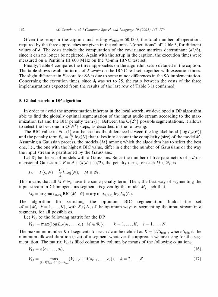
Figs. 5–8 plot F -score and execution time as functions of Smin, Kmax, Smax and d, respectively –each computed keeping fixed all the other parameters of the algorithm. In the followingconsiderations, the size of the parameters are sometimes in seconds, and not in number of ob-servations as usual: in these experiments 1 s of audio is represented by 100 observation vectors.

1 Experiments were performed on a Pentium III 1 GHz, 1 Gb RAM.

Table 5

Set-up of the global algorithm for the segmentation of the NIST data

Smin ¼ 75 Smax ¼ 1500 Kmax ¼ 80

d ¼ 5 k ¼ 0:60

Table 6

Set-up of the local (CSA) algorithm for the segmentation of the NIST data

Nmin ¼ 200 DNgrow ¼ 50 dl ¼ 25

Nmax ¼ 500 DNshift ¼ 100 dh ¼ 5

Nsecond ¼ 400 Nmargin ¼ 50 k ¼ 0:85

Table 7

Performance of the local and global algorithms on the NIST test set (0.3 s is the tolerance admitted in the change

detection)

Performance Execution time (s)

Precision Recall F -score Without BðÞLocal 54.4 75.7 63.3 367.7 –

Global 54.7 79.7 64.8 13,930.5 21,796.8

62.5

63

63.5

64

64.5

65

50 55 60 65 70 75 80 85 90 95 10013000

13500

14000

14500

15000

15500

F-S

CO

RE

(%

)

EX

EC

UT

ION

TIM

E (

SE

C)

F-SCORE

EXECUTION TIME

Fig. 5. F -score and execution time as functions of Smin.


Smin: It results that the value of the minimum window is critical, and the best value is not equalto the minimum size of test segments as expected (half a second, after the merging stage men-tioned in Section 3.2), but is slightly larger (0.75 s). Perhaps, that value could be – somehow –related to the tolerance used in the automatic evaluation procedure (0.3 s).

Kmax: The limit on the number of searched segments also affects accuracy when its value islower than a threshold (about 50). Since the average length of segments in the test set is 1.3 s, andthe audio files lasted about 1 min, the expected number of segments in each file is about 45, which

58

59

60

61

62

63

64

65

66

30 35 40 45 50 55 60 65 70 75 8013400

13500

13600

13700

13800

13900

14000

F-S

CO

RE

(%

)

EX

EC

UT

ION

TIM

E (

SE

C)

F-SCORE

EXECUTION TIME

Fig. 6. F -score and execution time as functions of Kmax.

64.6

64.65

64.7

64.75

64.8

64.85

64.9

0 1000 2000 3000 4000 5000 60004000

6000

8000

10000

12000

14000

16000

18000

20000

22000

F-S

CO

RE

(%

)

EX

EC

UT

ION

TIM

E (

SE

C)

F-SCOREEXECUTION TIME

Fig. 7. F -score and execution time as functions of Smax.


is compatible with the threshold observed in the experiments. This means that Kmax must becarefully chosen, taking into account the characteristics of audio under processing.

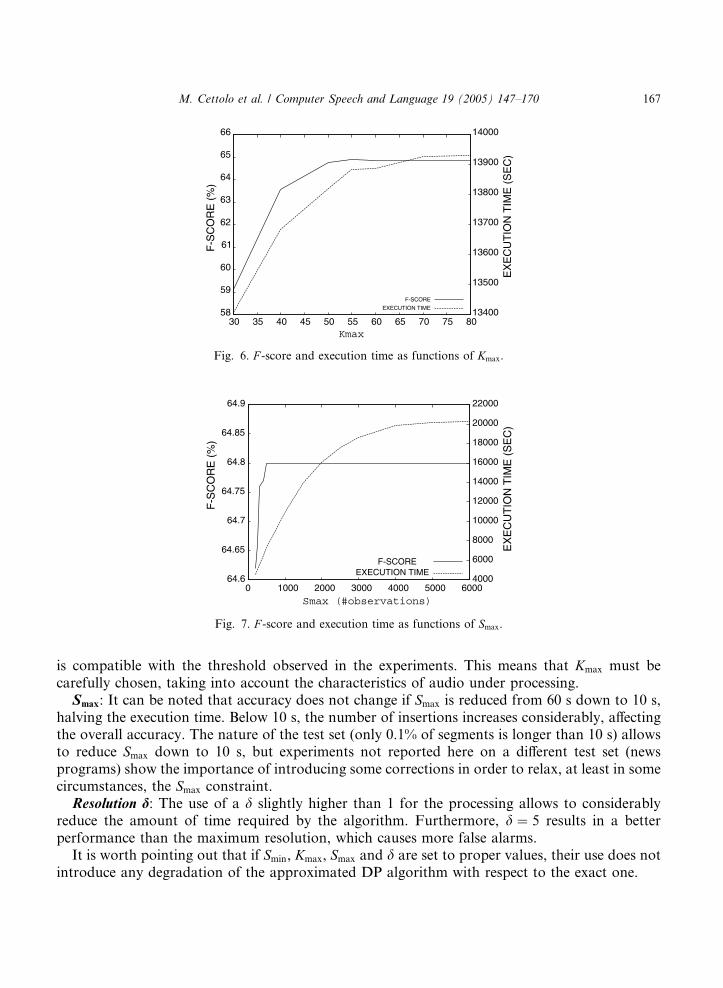
Smax: It can be noted that accuracy does not change if Smax is reduced from 60 s down to 10 s,halving the execution time. Below 10 s, the number of insertions increases considerably, affectingthe overall accuracy. The nature of the test set (only 0.1% of segments is longer than 10 s) allowsto reduce Smax down to 10 s, but experiments not reported here on a different test set (newsprograms) show the importance of introducing some corrections in order to relax, at least in somecircumstances, the Smax constraint.

Resolution d: The use of a d slightly higher than 1 for the processing allows to considerablyreduce the amount of time required by the algorithm. Furthermore, d ¼ 5 results in a betterperformance than the maximum resolution, which causes more false alarms.

It is worth pointing out that if Smin, Kmax, Smax and d are set to proper values, their use does notintroduce any degradation of the approximated DP algorithm with respect to the exact one.

Fig. 8. F -score and execution time as functions of d.

Table 8

Performance of the local (using both diagonal and full covariance matrices) and global algorithms on broadcast news

programs (tolerance¼ 0.5 s)

Performance Execution time (s)

Precision Recall F -score Without BðÞLocal (diagonal R) 82.5 84.4 83.5 16.3 –

Local 89.2 89.6 89.4 42.2 –

Global 92.9 86.8 89.8 4021.3 4771.7


For completeness, the global algorithm and the CSA implementation of the local one have alsobeen compared on the IBNC test set. Results are shown in Table 8 (rows local and global). Inthis case, the benefit of the global search over the local one is negligible, as it was expected giventhe audio characteristics of broadcast news recordings. The first row of the table refers to the CSAimplementation of the local search with the use of diagonal covariance matrices, instead of fullmatrices as in all the experiments reported so far. The rationale behind this trial is that it isgenerally recognized that Cepstral coefficients are reasonably uncorrelated and can be satisfac-torily modeled with diagonal-covariance Gaussians, which dramatically reduce computationalrequirements of our algorithms. Unfortunately, the impressive reduction in time costs (16.3 s vs.42.2) is paid with a 6.6% relative F -score decrease.

6. Summary

In this work, three different approaches to the implementation of the well-known local BIC-based audio segmentation algorithm have been beforehand analyzed: (i) a simple method that usesonly a sum and a square sum of the input vectors, in order to save computations in estimatingcovariance matrices on partially shared data; (ii) the approach proposed in Sivakumaran et al.(2001), that encodes the input signal with cumulative distributions; (iii) an innovative approach


that encodes the input signal in cumulative pair of sums. The two latter approaches provide abetter use of the typical approximation made in the algorithm, which is the computation of DBICvalues not on all observations, but at a lower resolution.

The three approaches have been compared both theoretically and experimentally: the proposednew approach has turned out to be the most efficient.

The local algorithm is heuristic, hence the quality of its solutions is only a lower bound on thequality of the solutions achievable by the BIC criterion. In order to discover if there is any roomof improvement within or outside the heuristics, we have developed a DP algorithm that, withinthe BIC model, finds a globally optimal segmentation of the input audio stream. In the paper, it isdescribed, analyzed, and experimentally compared with the local BIC-based algorithm.

The global algorithm yields a small but consistent improvement of performance, with respect tothe local one, while its time cost is definitely higher. Its computational complexity was reducedwithout affecting accuracy, by introducing some reasonable approximations, yielding a less thanreal time cost.

Summarizing, results show that no much further improvement is possible under the BIC cri-terion, fact that is important to be aware of. On the other side, experiments make evident that thelocal algorithm is able to segment an audio stream almost as well as the global algorithm is. Thatis, the sliding window approach is effective as an heuristics towards the BIC criterion objectivefunction. This encouraged us in proposing improvements to the implementation of the localsearch, providing a benchmark for possible future experimental work on segmentation.

Acknowledgements

The authors are grateful to Marcello Federico for his help in the mathematical formalization ofthe segmentation problem in terms of model selection. The authors also thank Helmer Strik,Alberto Pedrotti, and the anonymous referees for their suggestions on how to improve the ori-ginal version of the manuscript.

References

Akaike, H., 1977. On entropy maximization principle. In: Krishnaiah, P.R. (Ed.), Applications of Statistics. North-

Holland, Amsterdam, Netherlands, pp. 27–41.

Baxter, R.A., 1996. Minimum message length inference: theory and applications. Ph.D. Thesis, Department of

Computer Science Monash University, Clayton, Victoria, Australia.

Cettolo, M., Federico, M., 2000. Model selection criteria for acoustic segmentation. In: Proceedings of the ISCA

Automatic Speech Recognition Workshop, Paris, France.

Cettolo, M., Vescovi, M., 2003. Efficient audio segmentation algorithms based on the BIC. In: Proceedings of the

ICASSP, vol. VI, Hong Kong, pp. 537–540.

Cettolo, M., 2000. Segmentation, classification and clustering of an Italian broadcast news corpus. In: Proceedings of

the Sixth RIAO – Content-Based Multimedia Information Access – Conference, Paris, France.

Chen, S.S., Gopalakrishnan, P.S., 1998. Speaker, environment and channel change detection and clustering via the

Bayesian Information Criterion. In: Proceedings of the DARPA Broadcast News Transcription and Understanding

Workshop, Lansdowne, VA.


Delacourt, P., Kryze, D., Wellekens, C., 1999. Speaker-based segmentation for audio data indexing. In: Proceedings of

the ESCA ETRW Workshop Accessing Information in Spoken Audio, Cambridge, UK.

Federico, M., Giordani, D., Coletti, P., 2000. Development and evaluation of an Italian broadcast news corpus. In:

Proceedings of the Second International Conference on Language Resources and Evaluation (LREC), Athens,

Greece.

Frakes, W.B., Baeza-Yates, R., 1992. Information Retrieval: Data Structures and Algorithms. Prenctice-Hall,

Englewood Cliffs, NJ.

Gauvain, J.-L., Lamel, L., Adda, G., 1998. Partitioning and transcription of broadcast news data. In: Proceedings of

the ICSLP, Sidney, Australia, pp. 1335–1338.

Gish, H., Siu, M., Rohlicek, R., 1991. Segregation of speakers for speech recognition and speaker identification. In:

Proceedings of the ICASSP, vol. II, Toronto, Canada, pp. 873–876.

Hain, T., Johnson, S.E., Tuerk, A., Woodland, P.C., Young, S.J., 1998. Segment generation and clustering in the HTK

broadcast news transcription system. In: Proceedings of the DARPA Broadcast News Transcription and

Understanding Workshop, Lansdowne, VA.

Harris, M., Aubert, X., Haeb-Umbach, R., Beyerlein, P., 1999. A study of broadcast news audio stream segmentation

and segment clustering. In: Proceedings of the EUROSPEECH, vol. III, Budapest, Hungary, pp. 1027–1030.

IBNC, 2000. Available from: <http://www.elda.fr/catalogue/en/speech/S0093.html>.

Kemp, T., Schmidt, M., Westphal, M., Waibel, A., 2000. Strategies for automatic segmentation of audio data. In:

Proceedings of the ICASSP, vol. III, Istanbul, Turkey, pp. 1423–1426.

Lu, L., Li, S.Z., Zhang, H.-J., 2001. Content-based audio segmentation using support vector machines. In: Proceedings

of the ICME, Tokyo, Japan, pp. 956–959.

NIST, 2000. Available from: <www.nist.gov/speech/tests/spk/2000/>.

Scheirer, E., Slaney, M., 1997. Construction and evaluation of a robust multifeature speech/music discriminator. In:

Proceedings of the ICASSP, Munich, Germany, pp. 1331–1334.

Schwarz, G., 1978. Estimating the dimension of a model. The Annals of Statistics 6 (2), 461–464.

Seber, G.A.F., 1984. Multivariate Observations. John Wiley & Sons, New York, NY.

Siegler, M.A., Jain, U., Raj, B., Stern, R.M., 1997. Automatic segmentation, classification and clustering of broadcast

news audio. In: Proceedings of the DARPA Speech Recognition Workshop, Chantilly, VA.

Sivakumaran, P., Fortuna, J., Ariyaeeinia, A.M., 2001. On the use of the Bayesian Information Criterion in multiple

speaker detection. In: Proceedings of the EUROSPEECH, vol. II, Aalborg, Denmark, pp. 795–798.

Tritschler, A., Gopinath, R., 1999. Improved speaker segmentation and segments clustering using the Bayesian

Information Criterion. In: Proceedings of the EUROSPEECH, vol. II, Budapest, Hungary, pp. 679–682.

Vescovi, M., Cettolo, M., Rizzi, R., 2003. A DP algorithm for speaker change detection. In: Proceedings of the

EUROSPEECH, vol. IV, Geneva, Switzerland, pp. 2997–3000.

Wegmann, S., Zhan, P., Gillick, L., 1999. Progress in broadcast news transcription at Dragon systems. In: Proceedings

of the ICASSP, Phoenix, AZ, pp. 33–36.

Wellekens, C., 2001. Seamless navigation in audio files. In: Proceedings of the ITRW on Speaker Recognition, Crete,

Greece, pp. 9–12.

http://www.elda.fr/catalogue/en/speech/S0093.html

http://www.nist.gov/speech/tests/spk/2000/

evaluation of bic-based algorithms for audio segmentation · evaluation of bic-based algorithms for...

Documents