ETSI GS MEC-IEG 006 V1.1.1 (2017-01)

Mobile Edge Computing; Market Acceleration;

MEC Metrics Best Practice and Guidelines

Disclaimer

The present document has been produced and approved by the Mobile Edge Computing (MEC) ETSI Industry Specification Group (ISG) and represents the views of those members who participated in this ISG.

It does not necessarily represent the views of the entire ETSI membership.

GROUP SPECIFICATION

ETSI

ETSI GS MEC-IEG 006 V1.1.1 (2017-01) 2

Reference DGS/MEC-IEG006Metrics

Keywords MEC, KPI

ETSI

650 Route des Lucioles F-06921 Sophia Antipolis Cedex - FRANCE

Tel.: +33 4 92 94 42 00 Fax: +33 4 93 65 47 16

Siret N° 348 623 562 00017 - NAF 742 C

Association à but non lucratif enregistrée à la Sous-Préfecture de Grasse (06) N° 7803/88

Important notice

The present document can be downloaded from: http://www.etsi.org/standards-search

The present document may be made available in electronic versions and/or in print. The content of any electronic and/or print versions of the present document shall not be modified without the prior written authorization of ETSI. In case of any

existing or perceived difference in contents between such versions and/or in print, the only prevailing document is the print of the Portable Document Format (PDF) version kept on a specific network drive within ETSI Secretariat.

Users of the present document should be aware that the document may be subject to revision or change of status. Information on the current status of this and other ETSI documents is available at

https://portal.etsi.org/TB/ETSIDeliverableStatus.aspx

If you find errors in the present document, please send your comment to one of the following services: https://portal.etsi.org/People/CommiteeSupportStaff.aspx

Copyright Notification

No part may be reproduced or utilized in any form or by any means, electronic or mechanical, including photocopying and microfilm except as authorized by written permission of ETSI.

The content of the PDF version shall not be modified without the written authorization of ETSI. The copyright and the foregoing restriction extend to reproduction in all media.

© European Telecommunications Standards Institute 2017.

All rights reserved.

DECTTM, PLUGTESTSTM, UMTSTM and the ETSI logo are Trade Marks of ETSI registered for the benefit of its Members. 3GPPTM and LTE™ are Trade Marks of ETSI registered for the benefit of its Members and

of the 3GPP Organizational Partners. GSM® and the GSM logo are Trade Marks registered and owned by the GSM Association.

ETSI

ETSI GS MEC-IEG 006 V1.1.1 (2017-01) 3

Contents

Intellectual Property Rights ................................................................................................................................ 5

Foreword ............................................................................................................................................................. 5

Modal verbs terminology .................................................................................................................................... 5

Introduction ........................................................................................................................................................ 5

1 Scope ........................................................................................................................................................ 6

2 References ................................................................................................................................................ 6

2.1 Normative references ......................................................................................................................................... 6

2.2 Informative references ........................................................................................................................................ 6

3 Definitions and abbreviations ................................................................................................................... 7

3.1 Definitions .......................................................................................................................................................... 7

3.2 Abbreviations ..................................................................................................................................................... 8

4 Metrics ...................................................................................................................................................... 9

4.1 General ............................................................................................................................................................... 9

4.2 Latency ............................................................................................................................................................. 10

4.2.1 General ........................................................................................................................................................ 10

4.2.2 Round-Trip Time ........................................................................................................................................ 10

4.2.3 One-Way Delay (OWD) ............................................................................................................................. 11

4.2.4 Set-up Time ................................................................................................................................................ 11

4.2.5 Service Processing Time ............................................................................................................................. 11

4.2.6 Context-update time .................................................................................................................................... 12

4.3 Energy efficiency ............................................................................................................................................. 12

4.4 Network throughput ......................................................................................................................................... 13

4.5 System resource footprint ................................................................................................................................. 14

4.5.1 General ........................................................................................................................................................ 14

4.5.2 Computational load ..................................................................................................................................... 14

4.5.3 Non user data volume exchange ................................................................................................................. 14

4.6 Quality .............................................................................................................................................................. 14

4.6.1 General ........................................................................................................................................................ 14

4.6.2 Objective and service-independent metrics about quality........................................................................... 14

4.6.3 Objective and service-dependent metrics about quality .............................................................................. 15

4.6.4 Subjective and service-dependent metrics about quality ............................................................................ 15

4.6.5 Objective metrics about user comfort ......................................................................................................... 15

5 Measurement methodology .................................................................................................................... 16

5.1 General ............................................................................................................................................................. 16

5.2 Evaluation of latency ........................................................................................................................................ 16

5.2.0 Introduction................................................................................................................................................. 16

5.2.1 Measurement methodology ......................................................................................................................... 17

5.2.1.1 Peak workload test ................................................................................................................................ 17

5.2.1.2 Uniform workload tests ......................................................................................................................... 17

5.2.1.3 Stress tests ............................................................................................................................................. 17

5.2.2 Latency measurement setup 1: passive measurements at the terminal ....................................................... 17

5.2.3 Latency measurement setup 2: passive measurements by probes ............................................................... 18

5.2.4 Latency measurement setup 3: active measurements .................................................................................. 19

5.3 Evaluation of energy efficiency ........................................................................................................................ 19

5.3.1 Introduction................................................................................................................................................. 19

5.3.2 Measurement methodology ......................................................................................................................... 20

5.3.2.1 General .................................................................................................................................................. 20

5.3.2.2 Energy efficiency measurement setup 1 (network side) ........................................................................ 20

5.3.2.2.1 General considerations .................................................................................................................... 20

5.3.2.2.2 Baseline: measurement without the MEC Server ............................................................................ 21

5.3.2.2.3 Frontline: measurement with the MEC Server ................................................................................ 21

5.3.2.2.4 Computation of EE gains ................................................................................................................. 21

5.3.2.3 Energy efficiency measurement setup 2 (terminal side) ....................................................................... 22

ETSI

ETSI GS MEC-IEG 006 V1.1.1 (2017-01) 4

5.3.2.3.1 General considerations .................................................................................................................... 22

5.3.2.3.2 Baseline: measurement without the MEC Server ............................................................................ 22

5.3.2.3.3 Frontline: measurement with the MEC Server ................................................................................ 22

5.3.2.3.4 Computation of EE gains ................................................................................................................. 23

5.4 Evaluation of network throughput .................................................................................................................... 23

5.4.1 General ........................................................................................................................................................ 23

5.4.2 Network throughput measurement setups ................................................................................................... 23

5.5 Evaluation of resource footprint ....................................................................................................................... 24

5.5.1 General ........................................................................................................................................................ 24

5.5.2 Computational load measurement setup 1: isolated execution environment .............................................. 24

Annex A (informative): Network Throughput Example ..................................................................... 25

Annex B (informative): Examples of metric value ranges .................................................................. 26

B.1 5G latency requirements ......................................................................................................................... 26

B.2 5G energy efficiency .............................................................................................................................. 26

Annex C (informative): POC#3 RAVEN - example of latency metric assessment ........................... 27

History .............................................................................................................................................................. 29

ETSI

ETSI GS MEC-IEG 006 V1.1.1 (2017-01) 5

Intellectual Property Rights IPRs essential or potentially essential to the present document may have been declared to ETSI. The information pertaining to these essential IPRs, if any, is publicly available for ETSI members and non-members, and can be found in ETSI SR 000 314: "Intellectual Property Rights (IPRs); Essential, or potentially Essential, IPRs notified to ETSI in respect of ETSI standards", which is available from the ETSI Secretariat. Latest updates are available on the ETSI Web server (https://ipr.etsi.org/).

Pursuant to the ETSI IPR Policy, no investigation, including IPR searches, has been carried out by ETSI. No guarantee can be given as to the existence of other IPRs not referenced in ETSI SR 000 314 (or the updates on the ETSI Web server) which are, or may be, or may become, essential to the present document.

Foreword This Group Specification (GS) has been produced by ETSI Industry Specification Group (ISG) Mobile Edge Computing (MEC).

Modal verbs terminology In the present document "shall", "shall not", "should", "should not", "may", "need not", "will", "will not", "can" and "cannot" are to be interpreted as described in clause 3.2 of the ETSI Drafting Rules (Verbal forms for the expression of provisions).

"must" and "must not" are NOT allowed in ETSI deliverables except when used in direct citation.

Introduction Mobile Edge Computing is a new technology that provides an IT service environment and cloud-computing capabilities at the edge of the mobile network, in close proximity to mobile subscribers. In order to make MEC a success and encourage network operators to deploy Mobile Edge (ME) systems as well as to make MEC attractive to application developers and service providers, it is necessary to demonstrate the benefits of this technology for fulfilling various requirements. In order to make MEC an attractive proposition for service providers and applications developers to host their applications on a ME Host instead of in a centralized cloud, it is important to demonstrate a quantifiable performance increase.

The present document describes a number of performance metrics which can be used to demonstrate the benefits of deploying services and applications on a ME Host compared to a centralized cloud or server. Examples of how these metrics can be measured are also described.

Examples of such metrics KPIs are reducing latency, increasing end-to-end energy efficiency and increasing network throughput.

ETSI

ETSI GS MEC-IEG 006 V1.1.1 (2017-01) 6

1 Scope The present document describes various metrics which can potentially be improved through deploying a service on a MEC platform. Example use cases are used to demonstrate where improvements to a number of key performance indicators can be identified in order to highlight the benefits of deploying MEC for various services and applications. Furthermore, the present document describes best practices for measuring such performance metrics and these techniques are further exemplified with use cases.

Metrics described in the present document can be taken from service requirements defined by various organizations (e.g. 5G service requirements defined by Next Generation Mobile Networks (NGMN) or 3rd Generation Partnership Project (3GPP)). An informative annex is used to document such desired and/or achieved ranges of performance which could be referenced from the main body of the present document.

2 References

2.1 Normative references References are either specific (identified by date of publication and/or edition number or version number) or non-specific. For specific references, only the cited version applies. For non-specific references, the latest version of the referenced document (including any amendments) applies.

Referenced documents which are not found to be publicly available in the expected location might be found at https://docbox.etsi.org/Reference.

NOTE: While any hyperlinks included in this clause were valid at the time of publication, ETSI cannot guarantee their long term validity.

The following referenced documents are necessary for the application of the present document.

[1] ETSI ES 202 706 (V1.4.1): "Environmental Engineering (EE); Measurement method for power consumption and energy efficiency of wireless access network equipment".

[2] ETSI ES 203 228 (V1.1.1): "Environmental Engineering (EE); Assessment of mobile network energy efficiency".

[3] ETSI GS MEC 002: "Mobile Edge Computing (MEC); Technical Requirements".

[4] ETSI GS MEC 001: "Mobile Edge Computing (MEC); Terminology".

[5] ETSI ES 202 336-12: "Environmental Engineering (EE); Monitoring and control interface for infrastructure equipment (power, cooling and building environment systems used in telecommunication networks); Part 12: ICT equipment power, energy and environmental parameters monitoring information model".

2.2 Informative references References are either specific (identified by date of publication and/or edition number or version number) or non-specific. For specific references, only the cited version applies. For non-specific references, the latest version of the referenced document (including any amendments) applies.

NOTE: While any hyperlinks included in this clause were valid at the time of publication, ETSI cannot guarantee their long term validity.

The following referenced documents are not necessary for the application of the present document but they assist the user with regard to a particular subject area.

[i.1] IETF RFC 4656: "One way active measurement protocol".

[i.2] IETF RFC 5357: "A two-way active measurement protocol".

ETSI

ETSI GS MEC-IEG 006 V1.1.1 (2017-01) 7

[i.3] IETF IP Performance Metrics Working Group: IPPM status pages.

NOTE: Available at https://tools.ietf.org/wg/ippm/.

[i.4] IETF IP Performance Metrics Working Group: Charter.

NOTE: Available at https://tools.ietf.org/wg/ippm/charters.

[i.5] NGMN Alliance 5G White Paper version 1.0 (17 February 2015): "NGMN 5G White Paper".

NOTE: Available at https://www.ngmn.org/uploads/media/NGMN_5G_White_Paper_V1_0.pdf.

[i.6] J. S. Milton, J. Arnold, "Introduction to Probability and Statistics", McGraw-Hill Education, 4th Edition.

[i.7] P. Serrano, M. Zink, J. Kurose, "Assessing the fidelity of COTS 802.11 sniffers", IEEE INFOCOM 2009, Rio de Janeiro, Brazil, April 2009.

[i.8] P. Serrano, A. Garcia-Saavedra, G. Bianchi, A. Banchs, A. Azcorra, "Per-frame Energy Consumption in 802.11 Devices and its Implication on Modeling and Design," IEEE/ACM Transactions on Networking, vol.23, no.4, pp.1243-1256, Aug. 2015.

[i.9] N Vallina-Rodriguez, J Crowcroft, "Energy Management Techniques in Modern Mobile Handsets," IEEE Communications Surveys & Tutorials, 1-20.

[i.10] ETSI MEC PoC#3 RAVEN: "Radio aware video optimization in a fully virtualized network".

NOTE: Available at http://mecwiki.etsi.org/index.php?title=PoC_3_Radio_aware_video_optimization_in_a_fully_virtualized_network.

[i.11] ETSI GS MEC 015: "Mobile Edge Computing (MEC) Bandwidth Management API".

3 Definitions and abbreviations

3.1 Definitions For the purposes of the present document, the terms and definitions given in ETSI GS MEC 001 [4], ETSI ES 203 228 [2] and the following apply:

NOTE: For some background definitions for network level energy efficiency, see ETSI ES 203 228 [2].

Energy Efficiency (EE): relation between the useful output and energy/power consumption

mobile network coverage Energy Efficiency: ratio between the area covered by the network in the Mobile Network under investigation and the energy consumption

mobile network data Energy Efficiency: ratio between the performance indicator based on Data Volume and the energy consumption when assessed during the same time frame

mobile network energy consumption: overall energy consumption of equipment included in the MN under investigation

system resources: any kinds of entities to be shared to compose services including computing power, processor and accelerator loads, memory usage, storage, network, database and applications

NOTE: System resources can be considered as a set of coherent functions, network data objects or services, accessible through a server where such system resources reside on a single host or multiple hosts and are clearly identifiable.

ETSI

ETSI GS MEC-IEG 006 V1.1.1 (2017-01) 8

3.2 Abbreviations For the purposes of the present document, the following abbreviations apply:

3GPP 3rd Generation Partnership Project API Application Programming Interface BER Bit Error Rate CN Core Network CPU Central Processing Unit DC Direct Current EE Energy Efficiency eNB eNodeB GPS Global Positioning System ICMP Internet Control Message Protocol IDT Inter Departure Time IP Internet Protocol IPPM IP Performance Metrics KPI Key Performance Indicator ME Mobile Equipment MN Mobile Network MOS Mean Opinion Score MSL MEC-Specific Latency MSS Maximum Segment Size MTU Maximum Transmission Unit NGMN Next Generation Mobile Networks NRQA No Reference Quality Assessment NRT Non Real-Time NTP Network Time Protocol OS Operating System OWD One-Way Delay PA Power Amplifier PEAQ Perceptual Evaluation of Audio Quality PEVQ Perceptual Evaluation of Video Quality PLR Packet Loss Rate POC Proof Of Concept POLQA Perceptual Objective Listening Quality Assessment PSNR Peak Signal-to-Noise Ratio PSS Proportional Set Size PTP Precision Time Protocol QoS Quality of Service RAN Radio Access Network RAVEN Radio Aware Video optimization in a fully virtualized network RSS Resident Set Size RT Real-Time RTT Round-Trip Time SDT Service Delivery Time SGW Service GW SPT Service Processing Time SUT Set-Up Time TCP Transmission Control Protocol UD Update delay UDP User Datagram Protocol UE User Equipment USS Unique Set Size VSS Virtual Set Size

ETSI

ETSI GS MEC-IEG 006 V1.1.1 (2017-01) 9

4 Metrics

4.1 General This clause introduces the metrics considered by ETSI ISG MEC for the evaluation of improvements introduced by Mobile Edge Computing technologies. While clause 4 is describing all the different metrics considered (in separated clauses), clause 5 is organized similarly (with one clause corresponding to each metric in clause 4) in order to introduce the related measurement methodologies.

Generally MEC metrics are introduced with different purposes: evaluating the improvement given by MEC (as perceived by the end user), and assessing the benefits of different MEC deployment options (thus giving insights from a technologic point of view).

All metrics introduced in the present document can demonstrate the improvements of MEC solutions at least in the two following ways:

1) comparison between MEC and non-MEC solutions;

2) assessment of MEC deployments: comparison between different ME host positions within the network.

In both cases, the goal is not to compare different vendors or solution providers, but to assess the improvement of MEC introduction with respect to a traditional system (without MEC), e.g. in order to understand the different deployment options against the different use cases (e.g. by minimizing costs, maximizing benefits or flexibility).

For this reason, MEC metrics can be classified into two main groups: functional and non-functional metrics. For both categories (defined here below), metrics can be referred to different MEC use cases, as listed in IETF RFC 4656 [i.1], and the actual assessment of these metrics can depend on the particular service and/or application utilization:

1) Functional metrics are related to MEC performances impacting on user perception (often called also KPIs, key performances indicators):

- Examples of functional service performance KPIs include: latency (both end-to-end, and one-way), energy efficiency, throughput, goodput, loss rate (number of dropped packets), jitter, number of out-of-order delivery packets, QoS, and MOS. Each of the functional metrics should be defined on per service basis. Note that the latency in localization (time to fix the position) is different from latency in content delivery.

2) Non-functional metrics are related to the performance of the service in terms of deployment and management:

- Examples of non-functional metrics include: service lifecycle (instantiation, service deployment, service provisioning, service update (e.g. service scalability and elasticity), service disposal), service availability and fault tolerance (aka reliability), service processing/computational load, global ME host load, number of API request (more generally number of events) processed/second on ME host, delay to process API request (north and south), number of failed API request. The sum of service instantiation, service deployment, and service provisioning provide service boot-time.

In both cases, one could measure all the statistics over the above metrics. In fact, all metrics are in principle time-variable, and could be measured in a defined time interval and described by a profile over time or summarized through:

• the maximum value;

• mean and minimum value;

• standard deviation;

• the value of a given percentile;

• etc.

All MEC metrics assessments can be done by considering the overall system, or portions of that, according to the purpose of the measurement itself. An example below (figure 1) shows a mobile network system with ME host, and the different entities potentially involved in the assessment.

ETSI

ETSI GS MEC-IEG 006 V1.1.1 (2017-01) 10

Figure 1: Measuring MEC metrics

4.2 Latency

4.2.1 General

The concept of latency is wide and encompasses manifolds metrics: in communications, latency refers to a time-interval whose measurement quantifies the delay elapsed between any event and a consequent target effect. Even more, still in the communication domain, latency is useful to measure phenomena both in the control plane (e.g. set-up time or hand-over time) and in the data plane (e.g. transfer delay). The purpose of this clause is not to define all the latency metrics potentially relevant to the MEC solutions, but rather to highlight what type of latency metrics can be adopted (or newly defined) and their potential roles.

Referring to all the latency metrics in the clauses 4.2.2 to 4.2.6, it is assumed that an ideal synchronization holds across the nodes under test for measurements purposes.

Note that different Latency measurements have been specified in IETF RFC 4656 [i.1] and IETF RFC 5357 [i.2]. However, the latency definitions within the subsequent clauses are referring to latency measured on application level.

4.2.2 Round-Trip Time

Round-Trip Time (RTT): by referring to figure 1, it is defined as the time taken for a request (e.g. packet) generated from a terminal (a) to go to the destination, be updated or replied and travel back to (a), in conditions of ideal service capabilities (i.e. the server and/or terminal response time is supposed to be fixed and the RTT does not depend on the server/terminal computational load). Characteristics of RTT include:

1) Depending on the service type, the RTT might include very heterogeneous paths. Referring to figure 1:

- (a)-(c)-(a) in case of MEC client-server applications;

- (a)-(e)-(a) in case of non-MEC client-server applications;

ETSI

ETSI GS MEC-IEG 006 V1.1.1 (2017-01) 11

- (a)-(c)-(a') -(c)-(a) in case of MEC P2P applications;

- (a)-(e)-(a') -(e)-(a) in case of non-MEC P2P applications.

2) RTT is a variable which likely changes over time for the same station and is described by a RTT profile over time. RTT statistics might be summarized through: the maximum, mean and minimum value of RTT, the variance, the value of a given percentile, etc.

3) RTT might also vary throughout different stations (e.g. terminal (a) and terminal (a')). A statistical description of RTT can then be used to describe how much the latency is homogeneous across the terminals (RTT fairness). As an example, one could measure the maximum difference between the mean latencies achieved by two different terminals. RTT fairness would be important for applications such as the on-line gaming, where all the users need to have a relatively similar latency to deliver a fair behaviour.

RTT is meant to describe how efficient the flow of information is; it is useful to evaluate the benefit of MEC architecture.

4.2.3 One-Way Delay (OWD)

OWD can be defined as a delay of an application request (e.g. data packet) from a source application to a destination application on the user-plane. Formally, the OWD of the ith request (e.g. datagram) between two interfaces (source and destination) can be calculated as: OWD(i) = | t_source(i)) - t_destination(i) |. It is assumed that the timing between the source (e.g. user terminal) and destination (e.g. the ME host) is synchronized.

True OWD measurements require the capturing and time stamping of data packets at both ends of the connection link. This most often involves distributed and synchronized measurement nodes. The desired level of accuracy depends on the application.

4.2.4 Set-up Time

In case of a connection-oriented service from the user to the mobile edge application, also the initial signalling could initially affect the latency and should be then kept into account. For this purpose, the set-up time should be defined:

• Set-up Time (SUT) is defined as the time elapsed since the service request by the terminal (a) to get the first packet of information to it (a):

- In case a maximum number of simultaneous connections were set, a metric related to the blocking probability (or connection refusal) should be jointly considered - even if it is not directly a latency measurement.

The SUT metric holds wherever the source of information is placed (local cache, remote cache, central server, etc.) and whatever the signalling architecture is (ME host, signalling proxies, central server); it measures the time for the successful establishment of the service.

4.2.5 Service Processing Time

The last variable which influences the service latency (and which completes its description) is the service processing time - it is supposed ideal in RTT, hence neglected so far. The following metrics are meant to complete the description:

• Service Processing Time (SPT) is the time employed by the server (MEC or non-MEC) to process and fulfil a user request. It depends on manifolds variable (computational load).

• Service Delivery Time (SDT) is the time which is taken to a user request to reach the server, being processed and reach back the terminal.

• Update delay (UD) is the metric which describes the time (minimum/mean/maximum, etc.) required to have the servers updated with the relevant information. This is important for MEC services - which is often making use of local caching of the information - but also for non-MEC solutions.

ETSI

ETSI GS MEC-IEG 006 V1.1.1 (2017-01) 12

It is useful to monitor SPT in order to evaluate the processing and computing capabilities provided by the ME host; SPT is a non-functional metric. SDT puts together SPT and RTT (SDT=SPT+RTT); SDT is a functional metric since the RTT is included. UD measures a parameter which cannot be directly be measured at the terminal, but which heavily influences the quality and consistency of the applications. UD is a non-functional metric, and it is very suitable for assessing MEC solutions.

In general, considering the specific MEC architecture, additional metrics can be specifically defined for the comparison between MEC solutions. They can be named MEC-Specific Latency metrics (MSL).

MSL metrics are particularly important to support the optimization of the MEC architecture. MSL can include new custom metrics definitions which can apply only to a specific MEC architecture.

For example one could study how the SDT or the UD varies depending on the position of the MEC serving nodes. Additionally, MEC-specific metric could be defined: for example an interesting figure is the number of simultaneous requests that a central server can manage to update the MEC entities throughout the network architecture.

4.2.6 Context-update time

In order to support an effective provision of context-aware applications, such as e.g. device location, augmented reality, one key feature is the ability to make available in real time the application with the relevant information about the general context of the mobile user, including potential information not personally supplied by the user. Some key context variables are, e.g. the localization or any other information provided by the producer ME application.

To this aim, this metric is defined as the time between a certain key variable is updated at the terminal and the service is able to provide an updated state of the user based on the global context. This time should be small enough for a seamless operation of context-aware applications. The context-update time is intended as non-functional metric, since its impact is on the delay at application level, which is including also other delays, and it is the sum of the one way delay (OWD) plus the service processing time (SPT).

4.3 Energy efficiency Energy efficiency (EE) for mobile networks is currently defined in ETSI ES 202 706 [1] and ETSI ES 203 228 [2] and it expresses the relationship between consumed power (or energy) and the production of a certain selected basic KPI of interest.

KPI

power=η (1a)

As an example considering KPI = Traffic, an EE metric can be expressed in the following manner:

[J/bit]or [W/bps] traffic

power=η (1b)

and in this case it expresses the consumed watt of power per transferred traffic (in bps), or equivalently the energy per number of transferred bits.

Depending on the purpose of the evaluation, other KPIs are also possible.

As a general definition, EE is referred to the ability of a mobile system to perform a certain work (e.g. transmit a volume of traffic, or satisfying the QoS requirements for a certain service) by minimizing the power consumption. From this point of view, different kinds of EE metrics can be defined, depending on the scope of the assessment, and thus on the source of power consumption considered. In fact, EE can be defined:

• at component level (e.g. PA, chip, other components of network equipment or of a terminal, etc.);

• at node level (e.g. terminal, eNB, SGW, etc.);

• at network level (e.g. a set of nodes including or not terminals, only RAN equipment or including CN nodes, etc.).

ETSI

ETSI GS MEC-IEG 006 V1.1.1 (2017-01) 13

In particular, energy efficiency can be defined from a user perspective (thus measuring the mobile terminals power consumption) and/or from a network provider perspective (thus by considering parts of the network, or network equipment, or again the overall network).

By following the previous classifications, the energy efficiency at user equipment is defined as:

[J/bit]or [W/bps] UE

UEUE T

PEE = (1c)

where PUE is the power consumption of the mobile terminal(s) and TUE is the volume of traffic (at user level) transferred within a certain traffic session (assuming that, by definition, during that session all QoS requirements are satisfied).

Similarly, it is defined:

[J/bit]or [W/bps] NET

NETNET T

PEE = (1d)

as the energy efficiency at network side, where PNET is the power consumption of the mobile network (or a portion of the network) and TNET is the volume of traffic (at user level) transferred within a certain traffic session (assuming that, by definition, during that session all QoS requirements are satisfied).

As a consequence, since power consumption of terminals is a KPI directly perceived by end users, the consequent definition of EEUE is a functional metric, while EENET is a non-functional metric (the latter being related to the system efficiency, and not necessarily perceivable by the user). While the first one (EEUE) has direct impacts on the mobile terminals battery lifetime, E2E evaluations of the second metric (defined in ETSI ES 202 706 [1] and ETSI ES 203 228 [2]) are of a particular interest for mobile operators, in order to assess the efficiency sustainability of their networks from a operation point of view.

4.4 Network throughput Network has a clear influence on the quality perceived by the users while consuming some applications. Depending on the kind of application, different parameters and even thresholds could be taken into account.

Commonly, network throughput or bandwidth consumption are determinant in the sense that not having enough throughput starves the application with the needed payload to be executed. Apart from that, episodes of sporadic absence of enough throughput could be mitigated by means of buffering, with different impact depending on the duration of such event.

For instance, video applications present some requirements due to the resolution in which the video content is coded. Different resolutions imply distinct bit rates for streaming, and then different throughput requirements in the network. The network throughput is also relevant from a video application perspective to determine the starting time for video play-out. Typically video applications initially send burst of information to rapidly feeding the application players, trying to minimize the time the user takes to experience the content.

As mentioned before, events where the throughput level cannot be guaranteed can produce starvation of content in the players, then experiencing (re-)buffering times that can seriously impact the perception of the user.

Similar situations could happen with some other applications like gaming, software upgrade downloads, etc.

Network throughput is defined as measurement in terms bit rate units (e.g. kbps) at application level, in both upstream and downstream direction of the communication. Since this is a metric at application level, it is categorized as functional metric.

Throughput measurements could be performed both at transmitter side and at the receiver side. The latter case could also be referred as the network goodput.

This metric can serve as a basis for assessing Mobile Edge Computing Bandwidth Management API [i.11].

ETSI

ETSI GS MEC-IEG 006 V1.1.1 (2017-01) 14

4.5 System resource footprint

4.5.1 General

When implementing a service, it is relevant to analyse the amount of system resources consumed, both in terms of a node's capacity but also in terms of communication requirements. All the metrics considered here are non-functional.

4.5.2 Computational load

The processing/computational time/load measures the amount of CPU processing time or cycles, and memory usage (VSS, RSS, PSS and USS) a service requires to operate.

A service can also utilize the I/O resources (e.g. Ethernet), in which case, an overall system resource utilization score (combining compute, memory, and I/O resources) can be used to characterize service requirements in different conditions (light, medium, and high load).

As described in clause 4.1, computational load related metrics are considered to be non-functional.

4.5.3 Non user data volume exchange

A service deployed with MEC requires the coordination of the modules running across different elements, this including the exchange of non-user data between entities to e.g. support application and user mobility. This type of system resource consumption can be accounted for by measuring the non-user-data rate between the following entities:

• Between the ME host and the Radio Network Nodes.

• Between ME hosts.

• Between the ME host and the operational network management.

4.6 Quality

4.6.1 General

Traditionally, QoE measures the global system performance using both subjective and objective measures of customer satisfaction. Efficiency, ease of use, reliability, customer loyalty are some of the factors the QoE addresses. In addition to these, other aspects such as service costs, architecture security and user's privacy can be taken into account for a more comprehensive definition of QoE.

The QoE metrics strongly depend on the service/application under analysis. Since new services are implemented thanks to the flexibility of MEC, the definition of QoE metrics becomes a relevant aspect.

QoE metrics can be roughly classified into:

1) Objective and service-independent metrics about quality.

2) Objective and service-dependent metrics about quality.

3) Subjective and service-dependent metrics about quality.

4) Objective metrics about user comfort.

4.6.2 Objective and service-independent metrics about quality

In the first class (Objective and service-independent metrics about quality) the following ones can be mentioned:

1) The buffering time (usually expressed in seconds) involves pre-loading data into a certain area of memory so that the data can be accessed faster when the application needs it. The larger the buffering time, the higher the delay between the 'live' transmission and the playback. Buffer dimensioning is a critical parameter especially in media streaming but buffer can also be of great benefit to compensate network fluctuations.

ETSI

ETSI GS MEC-IEG 006 V1.1.1 (2017-01) 15

2) Packet loss rate (PLR) is a traditional metric in packet-based network and it can be referred to as an application independent metric. A good estimation of this parameter helps the transmitter to better tune (whenever possible) data encoding to suit channel conditions. A feedback channel from the receiver(s) to the source is required to collect meaningful information of the perceived received quality. If a TCP transmission is available, this channel is already present and a proper processing of ACK/NACK messages can help interpolate the PLR figure.

3) The Bit Error Rate (BER) is the number of bit errors divided by the total number of transferred bits during a particular time interval. Similar to PLR, it is application independent and it has the great benefit of providing an insight of the channel status. The BER can be also evaluated using stochastic (Monte Carlo) simulations. If a simple transmission channel model (e.g. Binary symmetric channel or additive white Gaussian noise), this parameter can also be calculated analytically.

4.6.3 Objective and service-dependent metrics about quality

Apart from these application-independent metrics, some application-specific metrics can also be devised (Objective and service-dependent metrics about quality). To define a proper QoE, in this case, applications should be first classified, for instance in the following categories:

1) Real-Time (RT) services.

2) Non Real-Time (NRT) services.

3) Video services.

Video services can belong to both RT and NRT services categories.

Once the service type has been selected, a proper QoE metric could thus be defined.

As an example, in the case of image and/or video transmission, the well-known Peak signal-to-noise ratio (PSNR) can be adopted as a precise metric to access the perceived quality of an image. This metric requires both the original and the received/compressed image as a term of comparison. Many metrics have been proposed, based on the PSNR, to estimate this parameter, without the original (available at the transmitter) sequence. These metrics are usually referred to as No-Reference Quality Assessment (NRQA) metrics. Architectures based on the estimation of the perceived quality based on the feedback on the sequence number of received packets have also been proposed. For a video streaming, a 'smoothness' metric can also be devised defined as the ease of watch a video content without stops caused by network congestion.

In case of RT- services, latency measured, as previously defined, would be used or custom-adapted.

In case of NRT services, specific metrics could be defined. For instance, in case of location-based services, precision might be adopted to refer to the quality of experience for positioning; in case of an image retrieval, the percentage of image matching would represent an effective score.

4.6.4 Subjective and service-dependent metrics about quality

The above mentioned techniques are referred to as objective metrics because it is possible to automatically evaluate them using a proper set of information (e.g. the number of transmitted and received packets). Other metrics involve the interaction with the final users and their subjective evaluation of the perceived quality (Subjective and service-dependent metrics about quality). Typically, the Mean Opinion Score (MOS) is one of the most adopted. The MOS is generated by averaging the results of a set of standard, subjective tests conducted over a set of final users. In order to have a statistically significant MOS, the set of users should be carefully defined. Other subjective metrics are POLQA (Perceptual Objective Listening Quality Assessment), PEVQ (Perceptual Evaluation of Video Quality) and PEAQ (Perceptual Evaluation of Audio Quality).

4.6.5 Objective metrics about user comfort

Finally, worthily, some additional metrics can describe the user comfort in accessing the services (Objective metrics about user comfort). For instance:

1) responsiveness is defined as the initial delay before the service reacts to the user request (e.g. a game starts) somehow similar to the 'buffering time' for video streaming - a latency metric;

ETSI

ETSI GS MEC-IEG 006 V1.1.1 (2017-01) 16

2) portability is defined as a metric to characterize the service quality when the user is moving from a local cell to another while using a MEC service.

5 Measurement methodology

5.1 General Each service has to be evaluated in different settings:

• Standalone: where both functional and non-functional metrics are evaluated in an isolated environment that does not necessarily include the ME host. The latter can be used as a baseline to benchmark the performance gain when the ME host is used as a function of different service placement (e.g. in core network, macro data centres).

EXAMPLE: Computational load can be measured for each individual services inside and outside of the MEC to identify the load.

• Integrated: where both functional and non-functional metrics are evaluated in a real scenario based on the composition of multiple individual services.

Measurements can be obtained using different approaches:

• Dedicated service monitoring tools that measures the relevant functional metrics, either by the service itself or externally, and apply both to MEC and non-MEC solutions. Such metrics can be exposed to the ME host as a means to learn the resulting utilization and performance.

• Common service monitoring inside the ME host that measures the non-functional metrics from each individual services.

• Service orchestrator inside the ME host that measures the service non-functional metrics.

Additional tools are needed to generate workload and challenge the service in terms of service scalability, availability/reliability.

5.2 Evaluation of latency

5.2.0 Introduction

MEC benefits on latency are expected to be particularly relevant in some of the use cases defined in ETSI GS MEC 002 [3]. For instance, in the following use cases the evaluation of latency are pivotal for the assessment of MEC benefits:

• Mobile video delivery optimization using throughput guidance for TCP (defined in clause A.2 of [3]).

• Local content caching at the mobile edge (defined clause A.3 of [3]).

• Security, safety, data analytics (defined in clause A.4 of [3]).

• Augmented reality, assisted reality, virtual reality, cognitive assistance (defined in clause A.5 of [3]).

• Gaming and low latency cloud applications (defined in clause A.6 of [3]).

• MEC edge video orchestration (defined in clause A.10 of [3]).

• Vehicle-to-infrastructure communication (defined in clause A.14 of [3]).

ETSI

ETSI GS MEC-IEG 006 V1.1.1 (2017-01) 17

5.2.1 Measurement methodology

5.2.1.1 Peak workload test

A single burst of workload of a specific type is transmitted in a very short duration of time. This test determines the service response variations where a sudden workload should be processed (in real-time).

5.2.1.2 Uniform workload tests

The same number of workloads of the same type is sent periodically to the service. This determines the service response time under a continuous load over a period of time.

5.2.1.3 Stress tests

A set of bursty workload with increasing rate is sent to the service. This determines the maximum service capacity.

5.2.2 Latency measurement setup 1: passive measurements at the terminal

According to what is defined in clause 4.2, both round-trip time and the set-up time need to be evaluated at terminal side and can be performed either in an "active" way (i.e. by implementing a testing protocol and procedure) or in a "passive" way (without requiring any ad-hoc procedure, just monitoring the traffic).

The passive monitoring has its main benefits in the straightforward approach - not requiring additional impact on the server side - and in the possibility to monitor the applications in real-conditions, independently of the specific architecture (MEC or non-MEC) and for a longer time (at the cost of energy consumption, for example).

However, the passive approach also brings some constraints:

• It cannot count on low-level signalling (e.g. ICMP packets).

• It has to recognize packets (respectively reply-packets in RTT and service packets in SUT) based on deep packet inspection, and based on the application awareness.

• The measurement solution cannot be a standard one (a standard testing protocol) suitable for any application, but rather cut on the specific application considered.

Based on these considerations, the passive setup is embodied by a test-mode of each specific application. The passive measurements could be also enriched by additional attributes related to the application (e.g. which server is delivering the service). So it is possible, in the end, to collect rich statistics, both on the RTT and on the SUTs, also correlated to the architectures service of the terminals over time.

The setup is particularly significant for those services in which the end-user perception is critical, for instance:

• Mobile video delivery optimization using throughput guidance for TCP (defined in clause A.2 of [3]).

• Augmented reality, assisted reality, virtual reality, cognitive assistance (defined in clause A.5 of [3]).

• Gaming and low latency cloud applications (defined in clause A.6 of [3]).

• Vehicle-to-infrastructure communication (defined in clause A.14 of [3]).

Passive measurements can be performed in several locations. Referring to figure 2, in latency measurement setup 1 they are done directly in the terminal (a).

ETSI

ETSI GS MEC-IEG 006 V1.1.1 (2017-01) 18

Figure 2: Example of passive measurement of latency

In this case it is possible to measure several parameters (i.e. RTT and SUT) closely related to the user experience. Passive measurements are dependent both on the Operating System (OS) used by the terminal and on the service under analysis. On the terminal side the capture is usually performed by a software (see figure 3) that records all the traffic thanks to a library linked to the network interface.

Figure 3: Example of passive measurement of latency at the terminal

The software that analyses the packets can be custom built on the service (that is, by fetching only predefined packets). Alternatively, the measurement can be carried out with a general purpose software that captures all the packets.

5.2.3 Latency measurement setup 2: passive measurements by probes

To overcome the performance problems related to the involvement of the mobile terminal in the measurements, an external probe (p) can be used (refer to figure 2). The probe is by definition an intermediate node between two communicating elements, and as such it cannot be perfectly aware of the actual reception of all the packets transferred between the two elements. Thus, in some cases the passive measurement by means of probes can be insufficient to understand the behaviour of the system.

This setup is suitable for measurement parameters which are observable by network probes, but not for other metrics as the processing time (defined in clause 4.2.5), unless software probes are used; differently from setup 1, it is suitable also for one-way delay measurements.

When viable, the measurement applies to any use-case listed in clause 5.2.

Network interface of the terminal

Library for network traffic capture

GUI for packets interpretation and

filtering

Software for packets analysis

ETSI

ETSI GS MEC-IEG 006 V1.1.1 (2017-01) 19

Depending on the addressed metric, several possible locations of the probe can be considered, and one or multiple probes simultaneously can be involved in the measurement. Depending on the use case considered, probes can be located in the terminal (a), or in the radio interface (p) or at base station side (b).

For non-MEC architecture, probes can be also located on the server side (e).

All the probed data, and in particular the captures on the ME host can be used for joint analyses, such as for OWD and to measure the service processing time (SPT). Obviously, when latency is evaluated by delays on different probes an appropriate synchronization procedure is required between the involved elements.

A synchronization protocol (such as NTP or PTP) is recommended where more than one data collecting element is considered, and based on the gathered data an appropriate bound will be set on the accuracy of the latency measurement, which will then determine the significant figures of the results. Furthermore, the ability of the probe to capture data should be assessed when either radio conditions suggest it or it is limited in resources, through e.g. the use of multiple independent probes [i.7]. To this aim, the quality of the link between the terminal, eNB and probe should be estimated throughout the measurement whenever possible.

If the objective of the measurement is to understand the impact of a certain variable (e.g. load) on performance, or to compare the performance of MEC vs. non-MEC, a proper design of experiment should be carried out [i.6] whenever possible, to support a sound statistical analysis of the obtained results.

When performing stand-alone measurements (i.e. no comparison vs. non-MEC), care should be taken when performing standard statistical analysis to guarantee that the precision of the delay measurements (even for the case of one probe) is appropriate. Performance metrics obtained over periods of time should be analysed with caution, as these cannot be assumed independent in general.

5.2.4 Latency measurement setup 3: active measurements

Most of the metrics defined in clause 4.2 can be computed by setups adopting active measurements; among them:

• Mobile video delivery optimization using throughput guidance for TCP (defined in clause A.2 of ETSI GS MEC 002 [3]).

• Augmented reality, assisted reality, virtual reality, cognitive assistance (defined in clause A.5 of ETSI GS MEC 002 [3]).

• Gaming and low latency cloud applications (defined in clause A.6 of ETSI GS MEC 002 [3]).

• MEC edge video orchestration (defined in clause A.10 of ETSI GS MEC 002 [3]).

• Vehicle-to-infrastructure communication (defined in clause A.14 of ETSI GS MEC 002 [3]).

Differently from the pure observation of passive measurements, active measurements methods inject so called probe traffic into the network at a traffic source and measure the outcomes at a probe traffic receiver. Hence, active measurement methods affect the network traffic.

In addition, simple ping tests using ICMP messages assess the average RTT latency of each communication link in the system.

NOTE: Active measurements can benefit from the adoption of specific protocols aimed at testing; for instance, the protocols defined by IETF IP Performance Metrics (IPPM) Working Group [i.3]. The description of the IPPM Working Group is defined in the charter [i.4].

5.3 Evaluation of energy efficiency

5.3.1 Introduction

MEC benefits can be assessed in different use cases which are defined in ETSI GS MEC 002 [3].

A few examples are given by:

• Gaming and low latency cloud applications (defined in clause A.6 of ETSI GS MEC 002 [3]).

ETSI

ETSI GS MEC-IEG 006 V1.1.1 (2017-01) 20

• Application computation off-loading (defined in clause A.23 of ETSI GS MEC 002 [3]).

• Radio network information generation in aggregation point (defined in clause A.21 of ETSI GS MEC 002 [3]).

• Mobile video delivery optimization using throughput guidance for TCP (defined in clause A.2 of ETSI GS MEC 002 [3]).

According to the different use case, different EE gains can be achieved in different parts of the MEC system.

Some examples include:

• For application computation off-loading are expected in the terminal (reduction of power consumption in the terminal).

• For gaming and low latency cloud applications, the benefits (to be compared with a system with remote application server) are expected mainly on network elements.

5.3.2 Measurement methodology

5.3.2.1 General

This clause is intended to provide a methodology for the measurement setup in order to assess the energy efficiencies of placing a ME host in the radio access network to enable low latency delivery of services and reduce backhaul.

There are several scenarios of measuring energy efficiencies. One note to consider is the implementation of the ME host can vary and this varies any result. However, the present document can serve as a guideline for determining how much energy could be saved by using a ME host.

The baseline is defined as a deployment without a MEC server in place and the methodology for the assessment foresees:

1) the injection of traffic from some users to a remote application server;

2) the measurement of the energy consumption of the elements involved in that system;

3) the computation of EE metrics as defined in clause 4.

Compared to the baseline system, the frontline foresees a MEC server within the RAN network. In this case, the energy consumption is computed by taking into account this additional element, but also by considering the saving due to application and services residing on the MEC Server.

5.3.2.2 Energy efficiency measurement setup 1 (network side)

5.3.2.2.1 General considerations

This measurement setup is applied to use case A.6 on "Gaming and low latency cloud applications" defined in ETSI GS MEC 002 [3], where savings on infrastructure are beneficial for the operator (in this case the EE is a non-functional metric). The usage of ME host for cloud applications has of course beneficial impacts on the user perceived QoE, but in the scope of the present metric (energy efficiency) it also helps reducing the power consumption of the communication network to run that particular service, since the endpoint of the backend application is closer to the user (thus requiring a shorter path), and also not involving anymore the remote datacentre.

In the following the measurement setup is described for baseline and frontline system, and the final step of the assessment of the EE metric at network side.

Power consumption and energy efficiency measurements of individual mobile network elements are described in several standards (for example ETSI ES 202 706 [1] for radio base stations). The present document describes energy consumption and MN energy efficiency measurements in operational networks, thus the measurement setup of the baseline system should be based on current ETSI ES 203 228 [2].

In particular, the Energy Consumption of the MN can be measured:

• by means of metering information provided by utility suppliers; or

ETSI

ETSI GS MEC-IEG 006 V1.1.1 (2017-01) 21

• by mobile network integrated measurement systems;

• moreover, sensors can be used to measure site and equipment energy consumption.

NOTE 1: Due to the nature of the measurements (at equipment or site level), the present methodology is valid for mobile network (MN) energy efficiency assessment both in virtualized and not virtualized environments.

NOTE 2: More detailed measurement methodology for virtualized environments (e.g. by assessing the different VMs in the cloud system) are not described in the present document, and left for future releases.

5.3.2.2.2 Baseline: measurement without the MEC Server

Figure 4 is showing an example of network cluster assessment in absence of MEC, where measurements of power consumption are done by means of external measurement tools (e.g. current clamps or more accurated tools). Power consumption of base stations should be assessed by using mobile network integrated measurement systems, when available according to ETSI ES 202 336-12 [5].

Figure 4: Measurement without the MEC Server

5.3.2.2.3 Frontline: measurement with the MEC Server

Figure 5 is showing an example of network cluster assessment in presence of MEC, where measurements of power consumption are done by means of external measurement tools (e.g. current clamps or more accurated tools). Power consumption of base stations should be assessed by using mobile network integrated measurement systems, when available according to ETSI ES 202 336-12 [5].

Figure 5: Measurement without the MEC Server

Note that in this case the traffic flow is not involving anymore the remote data centre, and thus it should not be included in the overall power budget.

5.3.2.2.4 Computation of EE gains

Since the goal is the energy performance of the network, energy efficiency is defined at network side, according to (1d) in clause 4.3. As a consequence:

• provided that in the two scenarios the same cloud gaming is serving the same number of users;

• given PNET,base the power consumption of the mobile network without MEC; and

• given PNET,front the power consumption of the mobile network without MEC; and

ETSI

ETSI GS MEC-IEG 006 V1.1.1 (2017-01) 22

• then, the EE gain in percentage is given by (PNET,base - PNET,front )/PNET,base.

5.3.2.3 Energy efficiency measurement setup 2 (terminal side)

5.3.2.3.1 General considerations

This measurement setup is applied to use case A.23 on "Application computation off-loading" defined in ETSI GS MEC 002 [3], where savings on terminal are beneficial for the end user (in this case the EE is a functional metric). This prolongs the battery life of the mobile device (IoT, phone, vehicle, etc.) and can be more appropriate to run on the MEC Server. In this case, the end-to-end system can be more efficient overall and can be a way for the operator to generate revenue. Again this would depend on the application that is off loaded off the phone.

In general, the energy consumption of a mobile handset depends on a number of parameters such as the operating system, use of GPS, screen, etc. [i.9]. In this way, great care has to be put in the measurement methodology, to guarantee repeatability of experiments and a fair comparison of results. In particular, not only other communication interfaces should be deactivated when running the measurements, but also certain energy-hungry components (e.g. screen). As with the case of delay, the precision of the considered instruments should be taken into consideration.

While certain platforms provide with real-time reporting of energy consumption of components and applications (e.g. Android apps), it is in general recommended to instrument the mobile phone (e.g. the methodology followed in [i.8]) to guarantee that the measurements do not correspond to unusual circumstances. Furthermore, the same measurement methodology should be repeated with at least two independent terminals (ideally, from two different vendors), so the performance differences cannot be associated with vendor-specific considerations.

Practically any performance figure of interest can be derived from the instantaneous power consumption (instantaneous: the timing resolution of the measurement device is one order of magnitude smaller than the minimum time between events of the communication protocol). If this is not achievable, average power consumption measurements should be taken under different scenarios, and post processing of the results (following a proper design of experiment) would result in meaningful figures.

5.3.2.3.2 Baseline: measurement without the MEC Server

Figure 6 illustrates an example of network assessment in absence of MEC, where measurements of power consumption of the mobile terminal are done by means of external measurement tools (e.g. a DC power source that substitutes the mobile battery and provides instantaneous measurements of the current consumption). Given the strong dependency of the power consumption of a terminal on the traffic sent and received [i.8], it is advisable the use of a probe to capture traffic so as to understand differences between repetitions (due to e.g. retransmissions).

Figure 6: Measurement without the MEC Server

5.3.2.3.3 Frontline: measurement with the MEC Server

Figure 7 illustrates the case of network assessment in presence of MEC, where the power consumption methodology is the same as in the previous case. As the transmission/reception pattern might be significantly different in this case, it is also advisable the use of a probe to capture traffic to understand differences in terms of power consumption between the MEC and non-MEC cases.

ETSI

ETSI GS MEC-IEG 006 V1.1.1 (2017-01) 23

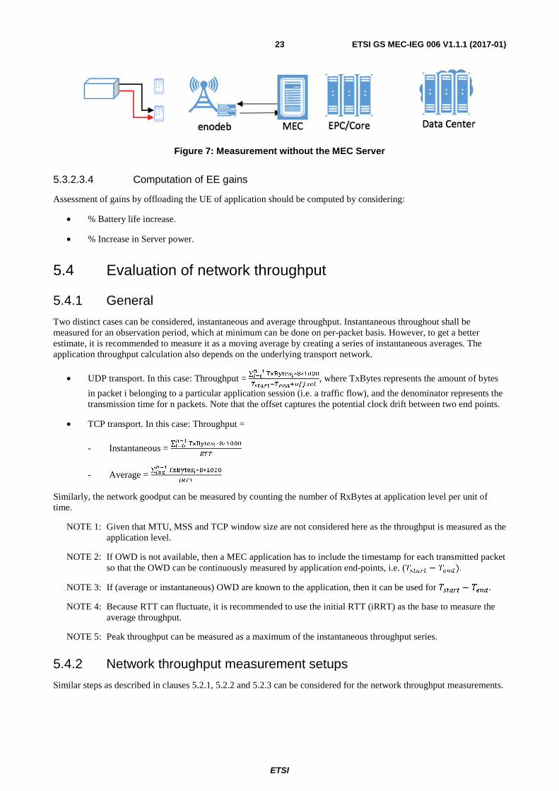
Figure 7: Measurement without the MEC Server

5.3.2.3.4 Computation of EE gains

Assessment of gains by offloading the UE of application should be computed by considering:

• % Battery life increase.

• % Increase in Server power.

5.4 Evaluation of network throughput

5.4.1 General

Two distinct cases can be considered, instantaneous and average throughput. Instantaneous throughout shall be measured for an observation period, which at minimum can be done on per-packet basis. However, to get a better estimate, it is recommended to measure it as a moving average by creating a series of instantaneous averages. The application throughput calculation also depends on the underlying transport network.

• UDP transport. In this case: Throughput = ∑ ��������������

∗∗����

��� �� �������, where TxBytes represents the amount of bytes

in packet i belonging to a particular application session (i.e. a traffic flow), and the denominator represents the transmission time for n packets. Note that the offset captures the potential clock drift between two end points.

• TCP transport. In this case: Throughput =

- Instantaneous = ∑ ��������������

∗∗����

�

- Average = ∑ ��������������

∗∗����

��

Similarly, the network goodput can be measured by counting the number of RxBytes at application level per unit of time.

NOTE 1: Given that MTU, MSS and TCP window size are not considered here as the throughput is measured as the application level.

NOTE 2: If OWD is not available, then a MEC application has to include the timestamp for each transmitted packet so that the OWD can be continuously measured by application end-points, i.e. (������ � �����.

NOTE 3: If (average or instantaneous) OWD are known to the application, then it can be used for ������ � ���� .

NOTE 4: Because RTT can fluctuate, it is recommended to use the initial RTT (iRRT) as the base to measure the average throughput.

NOTE 5: Peak throughput can be measured as a maximum of the instantaneous throughput series.

5.4.2 Network throughput measurement setups

Similar steps as described in clauses 5.2.1, 5.2.2 and 5.2.3 can be considered for the network throughput measurements.

ETSI

ETSI GS MEC-IEG 006 V1.1.1 (2017-01) 24

5.5 Evaluation of resource footprint

5.5.1 General

When comparing a MEC-enabled and Non-MEC system, two specific scenarios have to be considered:

• Baseline: where the computation load is measured without the ME host.

• Frontline: where the computation load is measured with the ME host.

Then the computation load is the relative difference (in percentage) between the two abovementioned scenarios.

In addition, the computation load can be assessed depending on the service placement strategy that can happen within the same or different ME hosts. Two scenarios are possible:

• Baseline: deployment A with placement strategy A.

• Frontline: deployment B with placement strategy B.

In any case the following procedure should be performed twice in order to assess the gain between the two abovementioned scenarios.

The processing/computational time/load of MEC service can be calculated using timestamps at the beginning and at the end of each MEC service or application. For instance "rdtsc" instruction or "clock_gettime" implemented on all x86 and x64 processors can be used to get a very precise timestamps. The "rdtsc" counts the number of CPU clocks since reset, while "clock_gettime" provides the current (physical) time. Therefore, the processing time is proportional to the value returned by the following pseudo-code:

1) s t a r t = start_meas ();

2) MEC_Service ( ) ; // execution of MEC service;

3) s t o p = stop_meas();

4) processing time = ( s t o p - s t a r t );

Primitives "start_meas" and "stop_meas" uses the underlying time measurement function to get the start and stop timestamp.

5.5.2 Computational load measurement setup 1: isolated execution environment

The simplest form to measure the computational load is to run a MEC service/application in an isolated execution environment (physical and virtual) allowing to characterize the behaviour of each individual function under different conditions and identify the bottlenecks.

ETSI

ETSI GS MEC-IEG 006 V1.1.1 (2017-01) 25

Annex A (informative): Network Throughput Example As a matter of example, table A.1 shows the throughput requirements of a very well-known application like Netflix™ (http://techblog.netflix.com/2015/12/per-title-encode-optimization.html).

NOTE: Netflix™ is the trade name of a product supplied by Netflix, Inc. This information is given for the convenience of users of the present document and does not constitute an endorsement by ETSI of the product named. Equivalent products may be used if they can be shown to lead to the same results.

Table A.1: Example throughput requirements

Bitrate (kbps) Resolution 235 320x240 375 384x288 560 512x384 750 512x384

1 050 640x480 1 750 720x480 2 350 1 280x720 3 000 1 280x720 4 300 1 920x1 080 5 800 1 920x1 080

ETSI

ETSI GS MEC-IEG 006 V1.1.1 (2017-01) 26

Annex B (informative): Examples of metric value ranges

B.1 5G latency requirements The following is captured from the NGMN 5G whitepaper [i.5] which describes user experience which include end-to-end latency requirements. The E2E latency as described in the NGMN 5G whitepaper [i.5] is the latency perceived by the end user and can be considered the same as Round Trip Time, which is defined in clause 4.2.2. These can be considered as latency value ranges to be considered for the performance of a service that utilizes a MEC deployment. A general requirement for the 5G system is it should be able to provide 10 ms E2E latency. Some use cases require extremely low latency which is considered to be either 1 ms or less. These latency targets make the assumption that the application layer processing time is negligible to the delay introduced by transport and switching. Various use case categories require different latency requirements. For instance, some use cases require ultra-low latency and also with the addition of ultra-high reliability or high throughput. Such use case categories require 1 ms or less.

MEC can contribute to the reduction of E2E latency.

B.2 5G energy efficiency The following is captured from the NGMN 5G whitepaper [i.5] which describes the energy efficiency requirements for network deployment, operation and management.

An energy efficiency increase of x 2 000 in the next 10 years timeframe is required for 5G networks. The rationale behind this requirement is the need for 5G to support a 1 000 times traffic increase in the next 10 years, but with an energy consumption of the whole network that is half of the typical energy consumption by today's networks.

MEC can contribute to a portion of these energy savings.

ETSI

ETSI GS MEC-IEG 006 V1.1.1 (2017-01) 27

Annex C (informative): POC#3 RAVEN - example of latency metric assessment The present annex is describing some latency measurements conducted in the framework of ETSI MEC PoC#3 RAVEN ("Radio aware video optimization in a fully virtualized network"). This proof-of-concept has been proposed in December 2015 to ETSI MEC [i.10] in accordance with PoC framework.

Figure C.1 shows the high-level scheme of PoC#3, that is aiming to demonstrate a video optimization application aware of the Radio conditions in the cell. The MEC application is co-located with eNB and communicating with video content server. The quality of video streams are adjusted according to radio conditions of the users. As a result, video streams and the quality perceived by users is improved thanks to the usage of MEC video optimization application.

Figure C.1: High-level scheme of PoC#3 RAVEN

The main steps of the demonstration are outlined below:

• UE1 sends a video stream to the video server.

• The server distributes the video stream to UE2 (and other users registered to the service).

• Once a congestion even occurs, a trigger is generated (through the MEC server) and the quality of video streams are adjusted according to radio conditions of the users.

Two main deployment options have been preliminarily evaluated in this PoC (and highlighted in figure C.2):

1) Video content server co-located with ME Host, and instantiated as a ME App.

2) Remote Video Content Server (located @ Politecnico di Torino premises), and far from eNB (instantiated @Eurecom premises).

Figure C.2: Steps of PoC#3 demonstration and different deployment options

ETSI

ETSI GS MEC-IEG 006 V1.1.1 (2017-01) 28

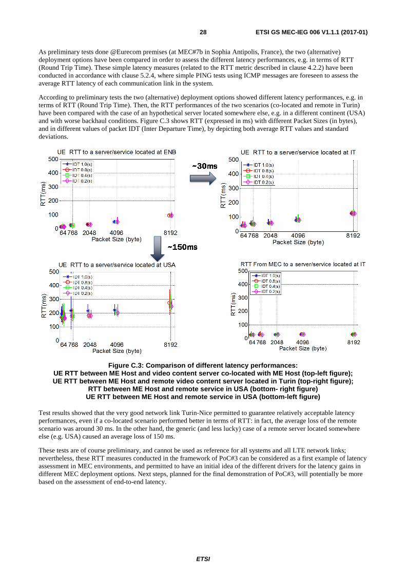
As preliminary tests done @Eurecom premises (at MEC#7b in Sophia Antipolis, France), the two (alternative) deployment options have been compared in order to assess the different latency performances, e.g. in terms of RTT (Round Trip Time). These simple latency measures (related to the RTT metric described in clause 4.2.2) have been conducted in accordance with clause 5.2.4, where simple PING tests using ICMP messages are foreseen to assess the average RTT latency of each communication link in the system.

According to preliminary tests the two (alternative) deployment options showed different latency performances, e.g. in terms of RTT (Round Trip Time). Then, the RTT performances of the two scenarios (co-located and remote in Turin) have been compared with the case of an hypothetical server located somewhere else, e.g. in a different continent (USA) and with worse backhaul conditions. Figure C.3 shows RTT (expressed in ms) with different Packet Sizes (in bytes), and in different values of packet IDT (Inter Departure Time), by depicting both average RTT values and standard deviations.

Figure C.3: Comparison of different latency performances: UE RTT between ME Host and video content server co-located with ME Host (top-left figure); UE RTT between ME Host and remote video content server located in Turin (top-right figure);

RTT between ME Host and remote service in USA (bottom- right figure) UE RTT between ME Host and remote service in USA (bottom-left figure)

Test results showed that the very good network link Turin-Nice permitted to guarantee relatively acceptable latency performances, even if a co-located scenario performed better in terms of RTT: in fact, the average loss of the remote scenario was around 30 ms. In the other hand, the generic (and less lucky) case of a remote server located somewhere else (e.g. USA) caused an average loss of 150 ms.

These tests are of course preliminary, and cannot be used as reference for all systems and all LTE network links; nevertheless, these RTT measures conducted in the framework of PoC#3 can be considered as a first example of latency assessment in MEC environments, and permitted to have an initial idea of the different drivers for the latency gains in different MEC deployment options. Next steps, planned for the final demonstration of PoC#3, will potentially be more based on the assessment of end-to-end latency.

ETSI

ETSI GS MEC-IEG 006 V1.1.1 (2017-01) 29

History

Document history

V1.1.1 January 2017 Publication