estimation of the 2d measurement error introduced by in-plane and out-of-plane electronic speckle...

*Tel.: 00 39 332 78 9237; fax: 00 39 332 78 6053; e-mail:[email protected] for Systems, Informatics and Safety, Advanced Technique for Information Analysis, Part-time

PhD Student, Department of Physics, University of Loughborough, Loughborough, UK.

Optics and Lasers in Engineering 31 (1999) 63}81

Estimation of the 2D measurement errorintroduced by in-plane and out-of-plane electronic

speckle pattern interferometry instruments

D. Albrecht*,1

European Commission, Joint Research Centre, Ispra Site, Via Fermi, 1, I-21020 Ispra, Italy

Received 14 May 1998; accepted 10 September 1998

Abstract

Optical interferometric metrology techniques are being increasingly used in industry. Thesetechniques assure a greater accuracy in measuring displacements caused by deformations. Onesuch technique, electronic speckle pattern interferometry (ESPI), has been used successfully tomeasure in-plane and out-of-plane deformations. The usual model describing ESPI instrumentsbehaviour is only valid in or near the centre of the illuminated surface. In general, this model isused as such for all the points on the surface creating thus an approximate "gure of the reality.This study has led to an improved 3D vectorial model, allowing us to assess qualitatively andquantitatively what is actually measured throughout all the inspected surface. Calculations withpractical parameters taken from real ESPI instruments designed in the Joint Research Centre ofIspra (Italy) were carried out. The results showing three-dimensional diagrams of the measure-ment errors are presented and discussed. ( 1999 Elsevier Science Ltd. All rights reserved.

1. Introduction

ESPI devices use light beams produced by coherent sources. In the 3D vectorialmodel, the point displacement d

x,yand the directions of the interfering beams are

described by vectors or unit vectors. The key idea is the point-by-point examination ofthe vectors characteristics that will tell exactly what is actually measured, and fromthere on the 2D measurement error can be drawn. In this paper, the same methodo-logy will be applied to an in-plane and an out-of-plane ESPI instrument. Features andresults particular to each type of instrument will be separately discussed.

0143-8166/99/$ - see front matter ( 1999 Elsevier Science Ltd. All rights reservedPII: S0143-8166(98)00043-8

Fig. 2. Out-of-plane instrument.

Fig. 1. In-plane instrument (only beam 1 is drawn).

ESPI devices exhibit a reference wavefront (IR) and an object wavefront (I

O*object

illumination). Most part of the illumination gets re#ected by the object externalsurface and proceeds backwards in the direction n

3of the viewing camera. When the

object is "xed, nothing happens. But when the object undergoes the e!ects of a force,most of the points on the surface are likely to move and according to the type ofinstrument, either one of the in-plane components d

1, d

2(in-plane instrument) or the

out-of-plane component d3

(out-of-plane instrument) of the total point displacementd"d

1#d

2#d

3will be measured (Figs. 1 and 2); a fringe pattern can be visualised.

64 D. Albrecht / Optics and Lasers in Engineering 31 (1999) 63}81

1.1. Geometric conxguration of an in-plane instrument

While keeping the next analysis very general, we will consider a typical in-planedevice oriented in the vertical direction, so that it will measure in-plane verticaldisplacements. In an ESPI in-plane device there are two illumination beams calledn1

and n2

placed symmetrically in respect to the optical axis. The origin of the3D coordinate system (i, j, k) is placed at A(0, 0, 0), the plane of the inspected arealies in i, j. The ESPI instrument optical axis is the bisector of the two illuminationbeams.

1.2. Geometric conxguration of an out-of-plane instrument

The expanding lens of the unique illumination beam n1

is located at the right-handside of the CCD camera.

A(0, 0, !wd) is the centre of the inspected area and wd stands for workingdistance.

The origin of the 3D coordinate system (i, j, k) is placed at O (0, 0, 0) centre of theCCD. The plane of the inspected area lies at z"!wd behind the i, j plane.

The optical axis acts as the reference for all the geometric parameters. To usea simple picture, the measurement device or its optical axis is assumed to bepositioned perpendicularly to the object surface. Vector k is aligned on the ESPIinstrument optical axis.

(d1"horizontal in-plane displacement, d

2"vertical in-plane displacement,

d3"out-of-plane displacement).Moreover from [1] we know that the phase change due to the point displace-

ment is:

for an in-plane instrument: *U"k (n1!n

2) ' d (1)

for an out-of-plane instrument *U"k (n1!n

3) ' d (2)

The total fringe pattern or its equivalent mathematical variable *U depends on j,(k"2n/j), and the combination (dot product) of the vectors n

1!n

2or n

1!n

3with

the displacement d"d1#d

2#d

3.

The real instrument parameters unfortunately do not correspond to the usualmodel:f one must consider all the illuminated surface, the illumination angle h

#is then not

constant and changes when the considered point sweeps over the inspected surface.f a 3D vectorial description must be used: n

i"k

1i#k

2j#k

3k,

f any displacement d must be considered, because during actual experiments, one cannever exclude the case of a real 3D displacement d"d

1#d

2#d

3.

This more exact "gure of the reality and the application of the above equationsallowed to "nd out that not only one component but all d

1, d

2, d

3components

unexpectedly contribute to the total fringe pattern. This can be a source of consider-able measurement errors.

D. Albrecht / Optics and Lasers in Engineering 31 (1999) 63}81 65

Fig. 3. Typical in-plane instrument parameters.

2. The total fringe pattern equations

2.1. In-plane instruments

2.1.1. The n and d vectorial equationsThe n

1, n

2vectors represent the illumination beams direction for each point in

the inspected area. Their direction is therefore di!erent at each considered point andtheir module is unity. For each point on the inspected area, there are thus a pair ofvectors n

1, n

2which when combined (dot product) with the local displacement

d"d1#d

2#d

3, will contribute to the total fringe pattern.

The optical axis is assumed to be perpendicular to the inspected surface. One cansee that the centre of the object is illuminated by the centre of the mirrors. The pointsof the object surface far from the centre are illuminated by points on the mirrors alsofar from the centre of the mirrors. To obtain more accurate results, one has decided totake into account the little and non-negligible shift, for example, of the origin of thevector N

1on the mirror M

1. A simple linear function was used to determine it (see the

Appendix).

In Fig. 3: xMi

, yMi

, zMi

: are the coordinates of the illuminating point of the mirrorM

i.

x.!9

, y.!9

: are the maximum coordinates of the illuminated points onthe inspected surface,

xM1

"0#x.1

; xM2

"0#x.2

;yM1

">1#y

.1; y

M2">

2#y

.2;

zM1

"Z1#z

.1; z

M2"Z

2#z

.2.

Xi, >

i, Z

iare "xed while x

.i, y

.i, z

.idepend on x

0"+%#5, y

0"+%#5, z

0"+%#5of

the measured point on the inspected surface (see the Appendix).


¹he n1

unit vector. The n1

unit vector describes the illumination beam vectorialcharacteristics coming from the mirror M

1, above the optical axis.

N1(x,y,z)

"(x0"+%#5

!xM1

) i#(y0"+%#5

!yM1

) j#(z0"+%#5

!zM1

)k

x0"+%#5

,x"coord. x of the point on the measured surface;y0"+%#5

,y"coord. y of the point on the measured surface;z0"+%#5

,z"coord. z"0, the origin of the coordinate system lies on the centreof the object plane.

DN1(x,y,z)

D"J (x0"+%#5

!xM1

)2#(y0"+%#5

!yM1

)2#(z0"+%#5

!zM1

)2

and

n1(x,y,z)

"

(x0"+%#5

!xM1

)

DN1D

i#(y

0"+%#5!y

M1)

DN1D

j#(z

0"+%#5!z

M1)

DN1D

k

Finally,

n1(x,y,z)

"

Ax0"+%#5

!

M1x0"+%#5

Dx.!9

D BDN

1D

i

#

A y0"+%#5

!A>1#AM1

sin(12n!h

#)

2 By0"+%#5

Dy.!9

D BBDN

1D

j

#

A z0"+%#5

!AZ1!AM1

cosC(12n!h

#)

2 DBy0"+%#5

Dy.!9

D BBDN

1D

k (3)

¹he n2

unit vector. The n2

unit vector describes the illumination beam vectorialcharacteristics coming from the mirror M

2, under the optical axis.

n2(x,y,z)

"

Ax0"+%#5

!

M2x0"+%#5

Dx.!9

D BDN

2D

i

#

A y0"+%#5

!AAAM2sin C

(12n!h

#)

2 DBy0"+%#5

Dy.!9

D B!>2BBDN

2D

j

#

A z0"+%#5

!AZ2#AAM2

cosC( 12n!h

#)

2 DBy0"+%#5

Dy.!9

D BBBDN

2D

k (4)

¹he d vector. The d vector describes the real displacement at each point of theinspected area. The typical case would be a vector in a direction pointed at 453 with


respect to the 3D reference coordinate axis (i, j, k). So

d(x,y,z)

"d1(x,y,z)

i#d2(x,y,z)

j#d3(x,y,z)

k (5)

2.1.2. The theoretical in-plane total fringe patternFrom Eq. (1); *U

(x,y,z)"k (n

1!n

2) ' d, and substituting Eqs. (3)} (5) in Eq. (1):

*U(x,y,z)

"kGC(x

0"+%#5!x

M1)

DN1D

i#(y

0"+%#5!y

M1)

DN1D

j#(z

0"+%#5!z

M1)

DN1D

kD!C

(x0"+%#5

!xM2

)

DN2D

i#(y

0"+%#5!y

M2)

DN2D

j#(z

0"+%#5!z

M2)

DN2D

kDH' (d1i#d

2j#d

3k)

Let us assume: M1"M

2"M; both mirrors have same diameter.

M:"(M sin[(n/2!h

#)/2]), and M

;"(M cos[(n/2!h

#)/2])

*U(x,y,z)

"

2nj G Ax0"+%#5

!

M x0"+%#5

Dx.!9

D BDN

1D

!

Ax0"+%#5!

M x0"+%#5

Dx.!9

D BDN

2D

i

#

Ay0"+%#5!A>1

#My

y0"+%#5

Dy.!9

DBBDN

1D

!

Ay0"+%#5

!AAMy

y0"+%#5

Dy.!9

DB!>2BBDN

2D

j

#

Az0"+%#5!AZ1!M

z

y0"+%#5

Dy.!9

DBBDN

1D

!

Az0"+%#5

!AZ2#M

z

y0"+%#5

Dy.!9

DBBDN

2D

k H' (d1

i#d2j#d

3k)

Finally,

*U(x,y,z)

"

4nj G 1

2

Ax0"+%#5!

M x0"+%#5

Dx.!9

D BDN

1D

!

Ax0"+%#5!

M x0"+%#5

Dx.!9

D BDN

2D

d1(x, y,z)

#

1

2

Ay0"+%#5!A>1#M

y

y0"+%#5

Dy.!9

DBBDN

1D


Fig. 4. Actual in-plane instrument dimensions.

!

Ay0"+%#5

!AAMy

y0"+%#5

Dy.!9

DB!>2BBDN

2D

d2(x,y,z)

#

1

2

Az0"+%#5!AZ1!M

z

y0"+%#5

Dy.!9

DBBDN

1D

!

Az0"+%#5

!AZ2#M

z

y0"+%#5

Dy.!9

DBBDN

2D

d3(x,y,z) H

N1

and N2

also depend on x, y, z and x0"+%#5

,x; y0"+%#5

,y; z0"+%#5

,z.

(6)

There is the "nal equation describing precisely the total fringe pattern or itsequivalent mathematical variable *U versus the displacement d and taking intoaccount the ESPI in-plane instrument geometrical parameters.

2.1.3. Application to an in-plane instrumentA real double in-plane instrument called ESPI

}I}10 was developed to inspect an

area of about 180]200 mm. Its dimensional con"guration shown hereafter willprovide the requested parameters to be included in Eq. (6) in order to assess the errorin the d

2displacement measurement and the error introduced by the possible unde-

sired d1, d

3displacements. The distances are expressed in mm (Fig. 4).


¹he ESPI}I}10 in-plane formula. From the appendix with Dx

.!9D"96 mm and

Dy.!9

D"80 mm:

M1"M

2"M"D/2"25 mm, M/ Dx

.!9D"25/96"0.260

m"(n/2!h#)/2"(90!15.4)/2"37.33

My"25 sin 37.3"15.15 mmPM

y/ Dy

.!9D"15.15/80"0.189

Mz"25 cos 37.3"19.88 mmPM

z/ Dy

.!9D"19.88/80"0.248

*U(x,y,z)

"

4p

j G1

2 C(x

0"+%#5!0.260x

0"+%#5)

DN1D

!

(x0"+%#5

!0.260x0"+%#5

)

DN2D D d

1(x,y,z)

#

1

2 C(y

0"+%#5!(>

1#0.189y

0"+%#5))

DN1D

!

(y0"+%#5

!( (0.189y0"+%#5

)!>2) )

DN2D D d

2(x,y,z)

#

1

2 C(z

0"+%#5!(Z

1!0.248y

0"+%#5) )

DN1D

!

(z0"+%#5

!(Z2#0.248y

0"+%#5) )

DN2D D d

3(x,y,z)Hand

DN1(x,y,z)

D"J0.546x20"+%#5

#(0.811 y0"+%#5

!190)2#(0.248 y0"+%#5

!690)2

and

DN2(x,y,z)

D"J0.546x20"+%#5

#(0.811 y0"+%#5

#180)2#(!0.248 y0"+%#5

!650)2

Finally, with z0"+%#5

"z"0:

*U(x,y)

"

4nj G

1

2 C0.739x

0"+%#5DN

1D

!

0.739x0"+%#5

DN2D D d

1(x,y)

#

1

2 C0.811 y

0"+%#5!190

DN1D

!

0.811 y0"+%#5

#180

DN2D D d

2(x,y)

#

1

2 C0.248y

0"+%#5!690

DN1D

!

!0.248 y0"+%#5

!650

DN2D D d

3(x,y)H (7)

N1

and N2

also depend on x, y, z and x0"+%#5

,x; y0"+%#5

,y; z0"+%#5

,z.


Fig. 5. Typical out-of-plane instrument parameters.

This is the "nal equation describing precisely the total fringe pattern obtained forall the inspected object surface with the ESPI

}I}10 in-plane instrument installed at

a working distance equal to 690 mm. Eq. (7) con"rms that not only d2

but also andunexpectedly d

1and d

3contribute to the total fringe pattern. The expressions within

the square brackets are the d1, d

2, d

3components coe$cients and are de"ned as d

1#,

d2#

, d3#

; Eq. (7)N*U(x,y)

"4n/j Md1#(x,y)

d1(x,y)

#d2#(x,y)

d2(x,y)

#d3#(x,y)

d3(x,y)

N.

2.2. Out-of-plane instruments

2.2.1. The n and d vectorial equationsThe n

1vector represents the illumination beam direction for each point in the

inspected area. Its direction is therefore di!erent at each considered point and itsmodule is unity.

For each point on the inspected area, there are thus the vectors n1

and n3

whichwhen combined (dot product) with the local displacement d"d

1#d

2#d

3, will

contribute to the total fringe pattern (Fig. 5).The optical axis is assumed to be perpendicular to the inspected surface. The

instrument is positioned at a certain distance from the object, the workingdistance (wd). Considering the case of a #at object, and disregarding the surfaceroughness, each point of the inspected area lies at the z coordinate equal to theworking distance (!wd). The origin of the coordinate system lies in the centre ofthe CCD.

¹he n1

unit vector. The n1

unit vector describes the illumination beam vectorialcharacteristics coming from the lens ¸ set at a distance e, on the right-hand side of the


optical axis:

N1(x,y,z)

"(x0"+%#5

!e)i#(y0"+%#5

!0)j#(z0"+%#5

!0)k

x0"+%#5



,z"coord. z of the point on the measured surface also called the workingdistance (wd)

DN1(x,y,z)

D"J(x0"+%#5

!e)2#y20"+%#5

#z20"+%#5

and

n1(x,y,z)

"

(x0"+%#5

!e)

DN1D

i#y0"+%#5DN

1D

j#z0"+%#5DN

1D

k (8)

The illumination beam gets expanded, thus some of the N1

vectors are issued fromsome point around the centre of the lens. To simplify the mathematical model, oneconsiders that all the N

1vectors join the centre of the lens ¸(e, 0, 0) to any point

(x, y, z) on the inspected surface, so N1

only depends on the x, y, z coordinates. Inpractice, the error thus introduced should not exceed 4/1000.

¹he n3unit vector. The n

3unit vector describes the imaging wavefront impinging on

the CCD camera.

N3(x,y,z)

"(0!x0"+%#5

) i#(0!y0"+%#5

) j#(0!z0"+%#5

)k

DN3(x,y,z)

D"Jx20"+%#5

#y20"+%#5

#z20"+%#5

x0"+%#5



,z"coord. z of the point on the measured surface also called the workingdistance (wd).

We can quickly "nd out the vectorial equation for the n3

unit vector:

n3(x,y,z)

"

!x0"+%#5

DN3D

i#!y

0"+%#5DN

3D

j#!z

0"+%#5DN

3D

k (9)

Though some of the N3

vectors reach a point around the centre of the CCD, oneconsiders that N

3joins any point (x, y, z) on the inspected surface to the centre of the

CCD, so N3

only depends on the x, y, z coordinates. In practice, the error thusintroduced should not exceed 4/1000.

¹he d vector. The d vector describes the real displacement at each point of theinspected area. The typical case would be a vector in a direction pointed at 453 withrespect to the 3D reference coordinate axis (i, j, k). So

d(x,y,z)

"d1(x,y,z)

i#d2(x,y,z)

j#d3(x,y,z)

k (10)


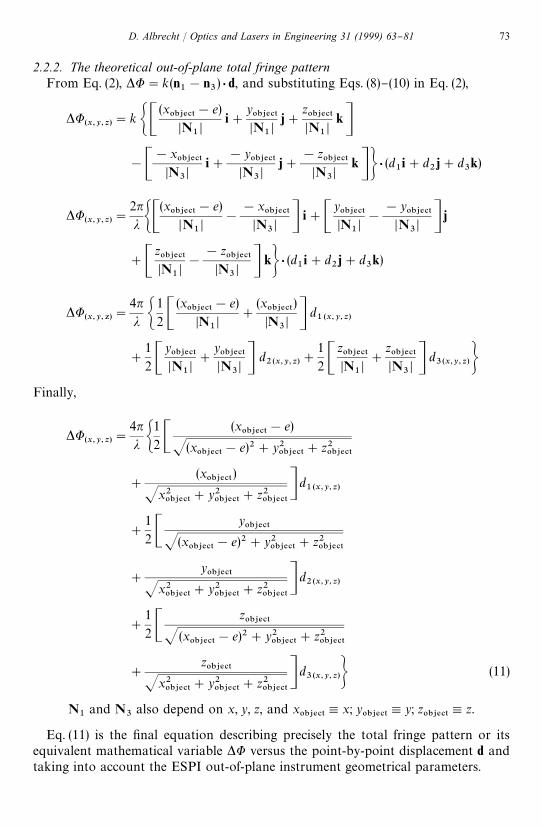
2.2.2. The theoretical out-of-plane total fringe patternFrom Eq. (2), *U"k(n

1!n

3) ' d, and substituting Eqs. (8)}(10) in Eq. (2),

*U(x,y,z)

"k GC(x

0"+%#5!e)

DN1D

i#y0"+%#5DN

1D

j#z0"+%#5DN

1D

kD!C

!x0"+%#5

DN3D

i#!y

0"+%#5DN

3D

j#!z

0"+%#5DN

3D

kDH ' (d1i#d

2j#d

3k)

*U(x,y,z)

"

2nj GC

(x0"+%#5

!e)

DN1D

!

!x0"+%#5

DN3D D i#C

y0"+%#5DN

1D!

!y0"+%#5

DN3D D j

#Cz0"+%#5DN

1D!

!z0"+%#5

DN3D D kH ' (d1i#d

2j#d

3k)

*U(x,y,;)

"

4nj G

1

2 C(x

0"+%#5!e)

DN1D

#

(x0"+%#5

)

DN3D D d

1(x,y,z)

#

1

2 Cy0"+%#5DN

1D#

y0"+%#5DN

3D D d

2(x,y,z)#

1

2 Cz0"+%#5DN

1D#

z0"+%#5DN

3D D d

3(x,y,z)HFinally,

*U(x,y,z)

"

4nj G

1

2 C(x

0"+%#5!e)

J(x0"+%#5

!e)2#y20"+%#5

#z20"+%#5

#

(x0"+%#5

)

Jx20"+%#5

#y20"+%#5

#z20"+%#5

D d1(x,y,z)

#

1

2 Cy0"+%#5

J(x0"+%#5

!e)2#y20"+%#5

#z20"+%#5

#

y0"+%#5

Jx20"+%#5

#y20"+%#5

#z20"+%#5

D d2(x,y,z)

#

1

2 Cz0"+%#5

J (x0"+%#5

!e)2#y20"+%#5

#z20"+%#5

#

z0"+%#5

Jx20"+%#5

#y20"+%#5

#z20"+%#5

D d3(x,y,z)H (11)

N1

and N3

also depend on x, y, z, and x0"+%#5

,x; y0"+%#5

,y; z0"+%#5

,z.

Eq. (11) is the "nal equation describing precisely the total fringe pattern or itsequivalent mathematical variable *U versus the point-by-point displacement d andtaking into account the ESPI out-of-plane instrument geometrical parameters.


Fig. 6. Actual out-of-plane instrument dimensions.

2.2.3. Application to an out-of-plane instrumentAn out-of-plane instrument called ESPI

}O}50 was developed to inspect an area of

about 520]440 mm. Its dimensional con"guration shown hereafter will provide therequested parameters to be included in Eq. (11), in order to assess the error in the d

3out-of-plane displacement measurement and the possible undesired d

1, d

2in-plane

displacement components. The distances are expressed in mm (Fig. 6).¹he ESPI

}O}50 out-of-plane formula. The distance e between the CCD axis and the

expanding lens axis equals 120 mm. The instrument is normally located at a workingdistance of 1 m (z

0"+%#5"!1000 mm). From Eq. (11):

*U(x,y,x)

"

4nj G

1

2C(x

0"+%#5!120)

J (xo"+%#5!120)2#y2

0"+%#5#10002

#

(x0"+%#5

)

Jx20"+%#5

#y20"+%#5

#10002D d1(x,y,z)

#

1

2 Cy0"+%#5

J (x0"+%#5

!120)2#y20"+%#5

#10002

#

y0"+%#5

Jx20"+%#5

#y20"+%#5

#10002D d2(x,y,z)

!

1

2 C1000

J (x0"+%#5

!120)2#y20"+%#5

#10002

#

1000

Jx20"+%#5

#y20"+%#5

#10002D d3(x,y,z)H (12)


There is the "nal equation of the ESPI}O}50 out-of-plane instrument installed at

a working distance of 1000 mm. Eq. (12) con"rms that not only d3

but also andunexpectedly d

1and d

2contribute to the total fringe pattern. As in Eq. (7), the

expressions within the square brackets are the d1, d

2, d

3components coe.cients and

are de"ned as d1#

, d2#

, d3#

.

3. The normalised sensitivity coe7cients

The displacement components coe.cients are the point of interest in Eqs. (7) and(12). However, the exact values of d

1#, d

2#, d

3#would not be very clear for the

understanding of the respective action of d"d1#d

2#d

3on the total fringe pattern

*U. We can overcome this di$culty by de"ning a reference value.In the in-plane case Eq. (7), we want to use the ESPI instrument to measure the

vertical in-plane displacement d2. We can observe that d

2#is not perfectly constant

and has a maximum value near the centre where d1#"d

3#"0. If we take this

maximum value d2#-.!9

as a reference value, divide each coe$cient d2#(9,y)

by d2#-.!9

andmultiply by 100, we wil obtain a value equal to 100% at the point of the maximumvalue and a lower value for d

2#elsewhere. It is clear that the new 3D map represents

the d2normalised sensitivity coe.cients map (d

2/!#(%) versus x, y), the vertical in-plane

2D measurement error, of the instrument.The same can be done for the coe$cients d

1#, d

3#using the same d

2c}maxvalue for the

division. Again the new 3D maps are the d1

and d3

displacement componentsnormalised sensitivity coe$cients, (d

1/!#versus x, y, and d

3/!#(%) versus x, y), of the

instrument in respect of the d2#-.!9

value.In the out-of-plane case Eq. (12), the same reasoning can be used. We want to use the

ESPI instrument to measure the out-of-plane displacement d3. We can observe thatd3#

is not perfectly constant and has a maximum value d3#-.!9

near the centre whered1#"d

2#"0. If we take this maximum value of d

3#-.!9as a reference value, divide each

coe$cient d3#(x,y)

by d3#-.!9

and multiply by 100, we will obtain a value equal to 100% atthe point of the maximum value and a lower value for d

3#elsewhere. It is clear that the

new 3D map represents the d3

normalised sensitivity coe.cients map (d3/!#

(%) versusx, y), the out-of-plane 2D measurement error, of the instrument.

The same can be done for the coe$cients d1#

, d2#

using the same d3#-.!9

value for thedivision. Again the new 3D maps are the d

1and d

2displacement components

normalised sensitivity coe$cients (d1/!#

versus x, y, and d2/4#

(%) versus x, y), of theinstrument in respect to the d

3#-.!9value.

In both case, *U is the sum of the negative and positive contributions of each of thed1, d

2, d

3displacement components multiplied by the respective components sensitivi-

ties of the instrument. The "nal result depends, on the working distance, on the pointto point d

1/4#(x,y), d

2/4#(x,y), d

3/4#(x,y), values of the instrument and on the real d

1(x,y), d

2(x,y), d

3(x,y),

displacement components occurring during the measurement. One can expect somevalues above 100%.

In the best case, the undesirable components are zero (vertical in-plane: d1"d

3"0)

and (out-of-plane: d1"d

2"0) or are negligible during the experiment. Another


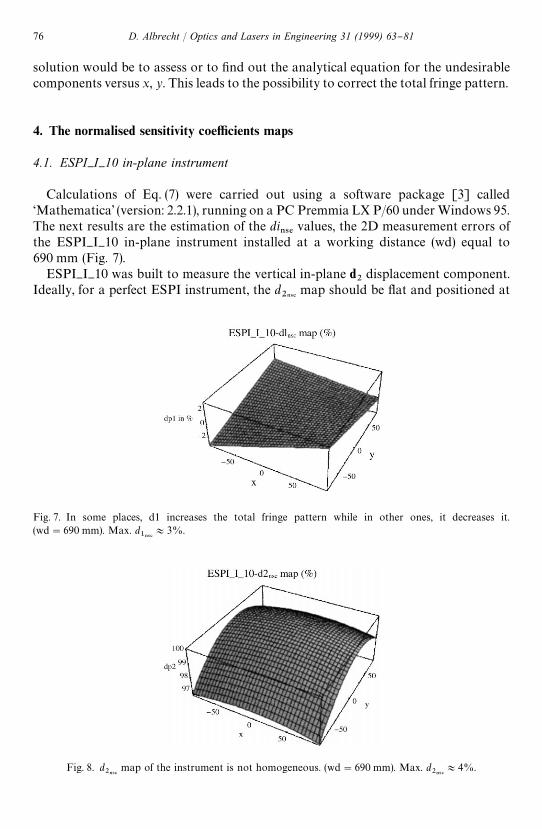
Fig. 8. d2/4#

map of the instrument is not homogeneous. (wd"690 mm). Max. d2/4#

+4%.

Fig. 7. In some places, d1 increases the total fringe pattern while in other ones, it decreases it.(wd"690 mm). Max. d

1/4#+3%.

solution would be to assess or to "nd out the analytical equation for the undesirablecomponents versus x, y. This leads to the possibility to correct the total fringe pattern.

4. The normalised sensitivity coe7cients maps

4.1. ESPI}I}10 in-plane instrument

Calculations of Eq. (7) were carried out using a software package [3] called&Mathematica' (version: 2.2.1), running on a PC Premmia LX P/60 under Windows 95.The next results are the estimation of the di

/4%values, the 2D measurement errors of

the ESPI}I}10 in-plane instrument installed at a working distance (wd) equal to

690 mm (Fig. 7).ESPI

}I}10 was built to measure the vertical in-plane d

2displacement component.

Ideally, for a perfect ESPI instrument, the d2/4#

map should be #at and positioned at


Fig. 9. When y'0, a d3'0 increases the total fringe pattern while in the y(0 region, it decreases it(wd"690 mm). Max. d

3/4#+8%.

Fig. 10. Sum of the d1/4#

, d2/4#

, d3/4#

values of the instrument for a wd"690 mm.

100% while the d1/4#

and d3/4#

maps should be #at and placed at 0%. Unfortunately,this is far to be the case; Fig. 8 is not homogeneous, Figs. 7 and 9 are not zero. Fig. 10is only illustrative and shows areas above and below 100%.

4.2. ESPI}O}

50 out-of-plane instrument

The next results are the estimation Eq. (12) of the di/4#

values, the 2D measurementerrors of the ESPI

}O}50 out-of-plane instrument installed at a working distance (wd)

equal to 1000 mm.ESPI

}O}50 was built to measure the out-of-plane d

3displacement component.

Ideally, for a perfect ESPI instrument, the d3/4#

map should be #at and positioned at100% while the d

1/4#and d

2/4#maps should be #at and placed at 0%. Unfortunately,


Fig. 11. A d1'0 increases the total fringe pattern when x(0, and when x'0 it decreases it.(wd"1000 mm). Max. d

1/4#+30%.

Fig. 12. When y'0, a d2'0 decreases the total fringe pattern while in the y(0 region, it increases it.(wd"1000 mm). Max. d

2/4#+20%.

Fig. 13. d3/4#

map of the instrument is not homogeneous. (wd"1000 mm). Max. d3/4#

+7%.


Fig. 14. Sum of the d1/4#

, d2/4#

, d3/4#

values of the instrument for a wd"1000 mm.

this is far to be the case; Fig. 13 is not homogeneous, Figs. 11 and 12 are not zero.Fig. 14 is only illustrative and shows areas above and below 100%.

5. Conclusions

The total fringe pattern generated on the screen is directly related to the globalphase di!erence *U that the illumination beam(s) undergo(es) when the point on thesurface moves. After a simple analysis using a vectorial approach, the fundamentalequation shows that the total fringe pattern change *U depends on the wavelength j,the unit vectors n

1, n

2(in-plane) or n

1, n

3(out-of-plane) and the displacement d.

Curiously in the case of the in-plane instrument, the n3

unit vector has no in#uence.The merit of the vectorial approach is that it is a very versatile method. It can easily

be used for any type of ESPI device as long as there are beams that can be describedby unit vectors.

Accurate three-dimensional vectorial analysis demonstrates that the instrument,though developed to measure a de"ned component (ex.: vertical in-plane d

2, out-of-

plane d3) of the total displacement, is unfortunately also sensitive to the other

components. More precisely, when the inspected point sweeps over the whole objectsurface, the vector n

1!n

2(in-plane) or the vector n

1!n

3(out-of-plane) often called

the sensitivity vector [1] is no longer vertical (vertical in-plane) or no longer perpen-dicular (to the i, j plane, out-of-plane); each non-perfectly vertical (in-plane) or perpen-dicular (out-of-plane) component of the sensitivity vector can combine (by the dotproduct) with the other components of the local displacement d and the real instru-ment is likely to be partially sensitive to those undesired displacement components, towit: d

1, d

3for vertical in-plane and d

1, d

2for out-of-plane.

This leads to the concept of displacement components sensitivity and more con-cretely to the drawing of normalised sensitivity coe$cients (d

i/4#) maps where the

values depend on the used working distance, and are characteristics of an ESPIinstrument. The coe$cients are expressed as percentages and are calculated in respect


to the maximum value of either the d1/4#

(horizontal in-plane) or the d2/4#

(verticalin-plane, ESPI

}I}10) or the d

3/4#(out-of-plane, ESPI

}O}50) coe$cient.

In the case of the in-house developed in-plane instrument (ESPI}I}10), at a well

de"ned point x, y near the centre of the inspected (illuminated) area, d1/4#

"d3/4#

"0,and d

2/4#reaches a maximum of 100%, the vertical in-plane displacement is read

correctly.As the inspected point gets farther from this particular point, d

2/4#slightly decreases and

the d1/4#

and d3/4#

coe$cients contribute negatively or positively to the total fringe pattern.The combination of the elliptically illuminated area and the 2D error maps pro"les

makes that the calculated extreme values are never reached. At a working distance of690 mm: d

2/4#coe$cient remains above 97%, only a maximum of about 1% of d1

(when present), and about 8% of d3

(when present) can be measured.In the case of the out-of-plane instrument (ESPI

}O}50), the d

3/4#coe$cient reaches

a maximum near the centre and then slowly decreases as it reaches the limits of theinspected area.

The 2D error done on the total fringe pattern is mainly introduced by thecontribution of the d

1and d

2in-plane displacement components. They act either

positively or negatively on the total fringe pattern; their contribution and so themeasured error is directly proportional to the inspected area size and inverselyproportional to the working distance. In the best case, at x"60, y"0,d1/4#

"d2/4#

"0, and the d3/4#

coe$cient reaches a maximum of 100%, the out-of-planedisplacement is read correctly. As the inspected point gets farther from the pointx"60, y"0, d

3/4#decreases while d

1/4#and d

2/4#increase.

At a working distance (wd) of 1 m, the performances of ESPI}O}50 are:

f d3: the essential component loses slightly its sensitivity and falls to a value of about

93%, it represents an error of &7%;f d

1: the horizontal in-plane component introduces (when present) a noticeable

amount of phase in the total fringe pattern. Normalised sensitivity coe$cient valuesfrom !20% to #30% are common;

f d2: the vertical in-plane component also introduces (when present) a noticeable

amount of phase in the total fringe pattern where the normalised sensitivitycoe$cient values extend from !22% to #22%.Other calculations led to the conclusion that the distance e between the CCD axis

and the lens axis has little e!ect (a couple of %) on the general performances of theinstrument. The increase of the working distance, however, improves greatly thequality of the measurements. For instance, when the ESPI

}O}50 instrument works at

2 m from the inspected surface, the in-plane normalised sensitivity coe$cients of thecomponents d

1and d

2are lowered by 50% compared to their value at 1 m.

It is clear that in any case the in-plane normalised sensitivity coe$cients are veryhigh for the ESPI

}O}50 out-of-plane instrument, and so it is, for any out-of-plane

ESPI device based on the same principle.For both types of instrument it is then important, when accurate measurements

must be carried out, to limit the inspection area size, to use the largest workingdistance possible and to avoid undesirable displacement components during measure-ment sessions.


Fig. 15. Detail of the mirror (in-plane).

Practical measurements carried out in laboratory are in very good agreement withthe developed theory. We have therefore shown the theoretical total fringe patternequations to be valid (Eqs. (6) and (11)).

Appendix

In Figs. 3 and 4, we can observe that a point located above point A(0, 0, 0), forexample, is no longer illuminated by the centre of the mirror but by a point slightlyabove the centre.

This progressive shift of the illuminating point along with the illuminated point andits precise x, y, z coordinates were calculated by a simple linear function as follows.From Figs. 3, 4 and 15:

Mi"D

i/2: D

iis the Mirror i diameter

xMi"M

ix0"+%#5

/Dx.!9

D: the linear function !x axisyMi">

i#[(M

isin[(n/2!h

#)/2]) (y/ Dy

.!9D )]: the linear function !y axis

ZMi"Z

i![(M

icos[(n/2!h

#)/2]) (y/ Dy

.!9D)]: the linear function !z axis

Acknowledgements

I would like to thank Ing. A.C. Lucia, Unit Head of the Modelling and AssessmentUnit, for his full support to this work. I am particularly grateful to Dr D. Emmony(Professor at the Loughborough University, England) for valuable guidance in thedevelopment of the ESPI devices.

References

[1] Jones R, Wykes C. Holographic and speckle interferometry. 2nd ed. Cambridge University Press, 1983.[2] Thomas GB, Finney RL. Calculus. 9th ed. Addison-Wesley, 1996.[3] Wolfram S, MathematicaTM, A System for doing Mathematics by Computer. Addison-Wesley, 1988.


estimation of the 2d measurement error introduced by in-plane and out-of-plane electronic speckle...

Documents